idl intro - faculty home pages
TRANSCRIPT

Introduction to IDL
Mark Piper, Ph.D.Michael D. Galloy, Ph.D.
RSI Global Services

Copyright © 2004-2005 Research Systems, Inc.All Rights Reserved.
IDL is a registered trademark of Research Systems, Inc. for the computer software described herein and its associated documentation. All other product names and/or logos are trademarks of their respective owners.
Version HistoryJuly 2004 First printing.September 2004 Revised, with minor edits.March 2005 Added glossary.October 2005 Updated for IDL 6.2.

iii

iv

Contents
1. About This Manual . . . . . . . . . . . . . . . . . . . . . . . . . . . . . . . . 1
Manual organization . . . . . . . . . . . . . . . . . . . . . . . . . . . . . . . . . . . . . . . . . . . . . . . . . . . . . . 2The course files . . . . . . . . . . . . . . . . . . . . . . . . . . . . . . . . . . . . . . . . . . . . . . . . . . . . . . . . . . . 3Chapter relationships . . . . . . . . . . . . . . . . . . . . . . . . . . . . . . . . . . . . . . . . . . . . . . . . . . . . . . 6Contacting RSI Global Services . . . . . . . . . . . . . . . . . . . . . . . . . . . . . . . . . . . . . . . . . . . . . . 6
2. A Tour of IDL . . . . . . . . . . . . . . . . . . . . . . . . . . . . . . . . . . . . . 7
Overview . . . . . . . . . . . . . . . . . . . . . . . . . . . . . . . . . . . . . . . . . . . . . . . . . . . . . . . . . . . . . . . . 8Scalars and arrays . . . . . . . . . . . . . . . . . . . . . . . . . . . . . . . . . . . . . . . . . . . . . . . . . . . . . . . . . 8Line plots . . . . . . . . . . . . . . . . . . . . . . . . . . . . . . . . . . . . . . . . . . . . . . . . . . . . . . . . . . . . . . . . 9Surface plots . . . . . . . . . . . . . . . . . . . . . . . . . . . . . . . . . . . . . . . . . . . . . . . . . . . . . . . . . . . . 11Contour plots . . . . . . . . . . . . . . . . . . . . . . . . . . . . . . . . . . . . . . . . . . . . . . . . . . . . . . . . . . . . 12Displaying and processing images . . . . . . . . . . . . . . . . . . . . . . . . . . . . . . . . . . . . . . . . . . 13IDL Intelligent Tools (iTools) . . . . . . . . . . . . . . . . . . . . . . . . . . . . . . . . . . . . . . . . . . . . . . 14Conclusion . . . . . . . . . . . . . . . . . . . . . . . . . . . . . . . . . . . . . . . . . . . . . . . . . . . . . . . . . . . . . . 14Exercises . . . . . . . . . . . . . . . . . . . . . . . . . . . . . . . . . . . . . . . . . . . . . . . . . . . . . . . . . . . . . . . . 14Suggested reading . . . . . . . . . . . . . . . . . . . . . . . . . . . . . . . . . . . . . . . . . . . . . . . . . . . . . . . 15
3. IDL Basics . . . . . . . . . . . . . . . . . . . . . . . . . . . . . . . . . . . . . . . 17
The IDL Development Environment . . . . . . . . . . . . . . . . . . . . . . . . . . . . . . . . . . . . . . . . 18IDL directory structure . . . . . . . . . . . . . . . . . . . . . . . . . . . . . . . . . . . . . . . . . . . . . . . . . . . 20IDL Online Help . . . . . . . . . . . . . . . . . . . . . . . . . . . . . . . . . . . . . . . . . . . . . . . . . . . . . . . . . 23Statements and programs . . . . . . . . . . . . . . . . . . . . . . . . . . . . . . . . . . . . . . . . . . . . . . . . . 23
vi
Batch files . . . . . . . . . . . . . . . . . . . . . . . . . . . . . . . . . . . . . . . . . . . . . . . . . . . . . . . . . . . . . . . 27Suggested reading . . . . . . . . . . . . . . . . . . . . . . . . . . . . . . . . . . . . . . . . . . . . . . . . . . . . . . . . 27
4. Graphics Systems . . . . . . . . . . . . . . . . . . . . . . . . . . . . . . . . .29
Direct Graphics vs. Object Graphics . . . . . . . . . . . . . . . . . . . . . . . . . . . . . . . . . . . . . . . . . 30Graphics windows in Direct Graphics . . . . . . . . . . . . . . . . . . . . . . . . . . . . . . . . . . . . . . . 30Color in Direct Graphics . . . . . . . . . . . . . . . . . . . . . . . . . . . . . . . . . . . . . . . . . . . . . . . . . . 33Exercises . . . . . . . . . . . . . . . . . . . . . . . . . . . . . . . . . . . . . . . . . . . . . . . . . . . . . . . . . . . . . . . . 38Suggested reading . . . . . . . . . . . . . . . . . . . . . . . . . . . . . . . . . . . . . . . . . . . . . . . . . . . . . . . . 38
5. IDL iTools . . . . . . . . . . . . . . . . . . . . . . . . . . . . . . . . . . . . . . . .39
An overview of the iTools . . . . . . . . . . . . . . . . . . . . . . . . . . . . . . . . . . . . . . . . . . . . . . . . . 40Interacting with iTools . . . . . . . . . . . . . . . . . . . . . . . . . . . . . . . . . . . . . . . . . . . . . . . . . . . . 44Getting help . . . . . . . . . . . . . . . . . . . . . . . . . . . . . . . . . . . . . . . . . . . . . . . . . . . . . . . . . . . . . 48Exercises . . . . . . . . . . . . . . . . . . . . . . . . . . . . . . . . . . . . . . . . . . . . . . . . . . . . . . . . . . . . . . . . 48Suggested reading . . . . . . . . . . . . . . . . . . . . . . . . . . . . . . . . . . . . . . . . . . . . . . . . . . . . . . . . 48
6. Line Plots . . . . . . . . . . . . . . . . . . . . . . . . . . . . . . . . . . . . . . . .51
Introduction . . . . . . . . . . . . . . . . . . . . . . . . . . . . . . . . . . . . . . . . . . . . . . . . . . . . . . . . . . . . . 52Plotting: Direct Graphics . . . . . . . . . . . . . . . . . . . . . . . . . . . . . . . . . . . . . . . . . . . . . . . . . . 52Plotting: iTools . . . . . . . . . . . . . . . . . . . . . . . . . . . . . . . . . . . . . . . . . . . . . . . . . . . . . . . . . . . 61Exercises . . . . . . . . . . . . . . . . . . . . . . . . . . . . . . . . . . . . . . . . . . . . . . . . . . . . . . . . . . . . . . . . 65Suggested reading . . . . . . . . . . . . . . . . . . . . . . . . . . . . . . . . . . . . . . . . . . . . . . . . . . . . . . . . 66
7. Variables . . . . . . . . . . . . . . . . . . . . . . . . . . . . . . . . . . . . . . . . .67
Introduction to variables . . . . . . . . . . . . . . . . . . . . . . . . . . . . . . . . . . . . . . . . . . . . . . . . . . 68Scalars . . . . . . . . . . . . . . . . . . . . . . . . . . . . . . . . . . . . . . . . . . . . . . . . . . . . . . . . . . . . . . . . . . 70Arrays . . . . . . . . . . . . . . . . . . . . . . . . . . . . . . . . . . . . . . . . . . . . . . . . . . . . . . . . . . . . . . . . . . 70Structures . . . . . . . . . . . . . . . . . . . . . . . . . . . . . . . . . . . . . . . . . . . . . . . . . . . . . . . . . . . . . . . 74Working with variables . . . . . . . . . . . . . . . . . . . . . . . . . . . . . . . . . . . . . . . . . . . . . . . . . . . 77System variables . . . . . . . . . . . . . . . . . . . . . . . . . . . . . . . . . . . . . . . . . . . . . . . . . . . . . . . . . 80Exercises . . . . . . . . . . . . . . . . . . . . . . . . . . . . . . . . . . . . . . . . . . . . . . . . . . . . . . . . . . . . . . . . 82Suggested reading . . . . . . . . . . . . . . . . . . . . . . . . . . . . . . . . . . . . . . . . . . . . . . . . . . . . . . . . 83
8. Surface and Contour Plots . . . . . . . . . . . . . . . . . . . . . . . . . .85
Displaying data as a surface plot . . . . . . . . . . . . . . . . . . . . . . . . . . . . . . . . . . . . . . . . . . . 86Displaying data with ISURFACE . . . . . . . . . . . . . . . . . . . . . . . . . . . . . . . . . . . . . . . . . . . 90Displaying data as a contour plot . . . . . . . . . . . . . . . . . . . . . . . . . . . . . . . . . . . . . . . . . . . 90Displaying data with ICONTOUR . . . . . . . . . . . . . . . . . . . . . . . . . . . . . . . . . . . . . . . . . . 93Combining contour and surface plots . . . . . . . . . . . . . . . . . . . . . . . . . . . . . . . . . . . . . . . 93Exercises . . . . . . . . . . . . . . . . . . . . . . . . . . . . . . . . . . . . . . . . . . . . . . . . . . . . . . . . . . . . . . . . 93Suggested reading . . . . . . . . . . . . . . . . . . . . . . . . . . . . . . . . . . . . . . . . . . . . . . . . . . . . . . . . 94

vii
9. Images . . . . . . . . . . . . . . . . . . . . . . . . . . . . . . . . . . . . . . . . . . 95
What is an image? . . . . . . . . . . . . . . . . . . . . . . . . . . . . . . . . . . . . . . . . . . . . . . . . . . . . . . . . 96Reading image data . . . . . . . . . . . . . . . . . . . . . . . . . . . . . . . . . . . . . . . . . . . . . . . . . . . . . . . 96Displaying an image . . . . . . . . . . . . . . . . . . . . . . . . . . . . . . . . . . . . . . . . . . . . . . . . . . . . . . 96Locating the origin of an image . . . . . . . . . . . . . . . . . . . . . . . . . . . . . . . . . . . . . . . . . . . . . 99Positioning an image in a window . . . . . . . . . . . . . . . . . . . . . . . . . . . . . . . . . . . . . . . . . 100Resizing an image . . . . . . . . . . . . . . . . . . . . . . . . . . . . . . . . . . . . . . . . . . . . . . . . . . . . . . . 101Reading images from the display . . . . . . . . . . . . . . . . . . . . . . . . . . . . . . . . . . . . . . . . . . 101Working with TrueColor (24-bit) images . . . . . . . . . . . . . . . . . . . . . . . . . . . . . . . . . . . . 104Writing or drawing on top of images . . . . . . . . . . . . . . . . . . . . . . . . . . . . . . . . . . . . . . . 106The device copy technique . . . . . . . . . . . . . . . . . . . . . . . . . . . . . . . . . . . . . . . . . . . . . . . . 108Suggested reading . . . . . . . . . . . . . . . . . . . . . . . . . . . . . . . . . . . . . . . . . . . . . . . . . . . . . . . 112
10. Programming . . . . . . . . . . . . . . . . . . . . . . . . . . . . . . . . . . 113
The Interactive Data Language . . . . . . . . . . . . . . . . . . . . . . . . . . . . . . . . . . . . . . . . . . . . 114Operators . . . . . . . . . . . . . . . . . . . . . . . . . . . . . . . . . . . . . . . . . . . . . . . . . . . . . . . . . . . . . . . 114Control statements . . . . . . . . . . . . . . . . . . . . . . . . . . . . . . . . . . . . . . . . . . . . . . . . . . . . . . . 117Procedures and functions . . . . . . . . . . . . . . . . . . . . . . . . . . . . . . . . . . . . . . . . . . . . . . . . . 121Documentation . . . . . . . . . . . . . . . . . . . . . . . . . . . . . . . . . . . . . . . . . . . . . . . . . . . . . . . . . . 123Exercises . . . . . . . . . . . . . . . . . . . . . . . . . . . . . . . . . . . . . . . . . . . . . . . . . . . . . . . . . . . . . . . 124Suggested reading . . . . . . . . . . . . . . . . . . . . . . . . . . . . . . . . . . . . . . . . . . . . . . . . . . . . . . . 124
11. File I/O . . . . . . . . . . . . . . . . . . . . . . . . . . . . . . . . . . . . . . . . 125
Binary and text files . . . . . . . . . . . . . . . . . . . . . . . . . . . . . . . . . . . . . . . . . . . . . . . . . . . . . . 126File manipulation routines . . . . . . . . . . . . . . . . . . . . . . . . . . . . . . . . . . . . . . . . . . . . . . . . 126High-level file routines . . . . . . . . . . . . . . . . . . . . . . . . . . . . . . . . . . . . . . . . . . . . . . . . . . . 128Low-level file routines . . . . . . . . . . . . . . . . . . . . . . . . . . . . . . . . . . . . . . . . . . . . . . . . . . . . 132IDL SAVE files . . . . . . . . . . . . . . . . . . . . . . . . . . . . . . . . . . . . . . . . . . . . . . . . . . . . . . . . . . 139Associated variables . . . . . . . . . . . . . . . . . . . . . . . . . . . . . . . . . . . . . . . . . . . . . . . . . . . . . 141Exercises . . . . . . . . . . . . . . . . . . . . . . . . . . . . . . . . . . . . . . . . . . . . . . . . . . . . . . . . . . . . . . . 142Suggested reading . . . . . . . . . . . . . . . . . . . . . . . . . . . . . . . . . . . . . . . . . . . . . . . . . . . . . . . 142
12. Analysis . . . . . . . . . . . . . . . . . . . . . . . . . . . . . . . . . . . . . . . 143
Introduction . . . . . . . . . . . . . . . . . . . . . . . . . . . . . . . . . . . . . . . . . . . . . . . . . . . . . . . . . . . . 144Interpolation . . . . . . . . . . . . . . . . . . . . . . . . . . . . . . . . . . . . . . . . . . . . . . . . . . . . . . . . . . . . 144Curve fitting . . . . . . . . . . . . . . . . . . . . . . . . . . . . . . . . . . . . . . . . . . . . . . . . . . . . . . . . . . . . 148Signal processing . . . . . . . . . . . . . . . . . . . . . . . . . . . . . . . . . . . . . . . . . . . . . . . . . . . . . . . . 151Image processing . . . . . . . . . . . . . . . . . . . . . . . . . . . . . . . . . . . . . . . . . . . . . . . . . . . . . . . . 154Exercises . . . . . . . . . . . . . . . . . . . . . . . . . . . . . . . . . . . . . . . . . . . . . . . . . . . . . . . . . . . . . . . 159Suggested reading . . . . . . . . . . . . . . . . . . . . . . . . . . . . . . . . . . . . . . . . . . . . . . . . . . . . . . . 160
13. Map Projections . . . . . . . . . . . . . . . . . . . . . . . . . . . . . . . . 161
Map projections . . . . . . . . . . . . . . . . . . . . . . . . . . . . . . . . . . . . . . . . . . . . . . . . . . . . . . . . . 162

viii
Creating a map projection . . . . . . . . . . . . . . . . . . . . . . . . . . . . . . . . . . . . . . . . . . . . . . . . 162Displaying data on a map projection . . . . . . . . . . . . . . . . . . . . . . . . . . . . . . . . . . . . . . . 163Converting data between map projections . . . . . . . . . . . . . . . . . . . . . . . . . . . . . . . . . . 167The iMap iTool . . . . . . . . . . . . . . . . . . . . . . . . . . . . . . . . . . . . . . . . . . . . . . . . . . . . . . . . . 169Exercises . . . . . . . . . . . . . . . . . . . . . . . . . . . . . . . . . . . . . . . . . . . . . . . . . . . . . . . . . . . . . . . 170Suggested reading . . . . . . . . . . . . . . . . . . . . . . . . . . . . . . . . . . . . . . . . . . . . . . . . . . . . . . . 171
14. Strings . . . . . . . . . . . . . . . . . . . . . . . . . . . . . . . . . . . . . . . . .173
Special characters and string operators . . . . . . . . . . . . . . . . . . . . . . . . . . . . . . . . . . . . . 174Summary of string routines . . . . . . . . . . . . . . . . . . . . . . . . . . . . . . . . . . . . . . . . . . . . . . . 174String functions . . . . . . . . . . . . . . . . . . . . . . . . . . . . . . . . . . . . . . . . . . . . . . . . . . . . . . . . . 175Regular expression searching and splitting . . . . . . . . . . . . . . . . . . . . . . . . . . . . . . . . . 178Exercises . . . . . . . . . . . . . . . . . . . . . . . . . . . . . . . . . . . . . . . . . . . . . . . . . . . . . . . . . . . . . . . 181Suggested reading . . . . . . . . . . . . . . . . . . . . . . . . . . . . . . . . . . . . . . . . . . . . . . . . . . . . . . . 182
15. Graphics Devices . . . . . . . . . . . . . . . . . . . . . . . . . . . . . . .183
IDL graphics devices . . . . . . . . . . . . . . . . . . . . . . . . . . . . . . . . . . . . . . . . . . . . . . . . . . . . 184Steps to output to a graphics device . . . . . . . . . . . . . . . . . . . . . . . . . . . . . . . . . . . . . . . . 185Configuring a graphics device . . . . . . . . . . . . . . . . . . . . . . . . . . . . . . . . . . . . . . . . . . . . 187Exercises . . . . . . . . . . . . . . . . . . . . . . . . . . . . . . . . . . . . . . . . . . . . . . . . . . . . . . . . . . . . . . . 192Suggested reading . . . . . . . . . . . . . . . . . . . . . . . . . . . . . . . . . . . . . . . . . . . . . . . . . . . . . . . 192
Glossary . . . . . . . . . . . . . . . . . . . . . . . . . . . . . . . . . . . . . . . . . .197
Index . . . . . . . . . . . . . . . . . . . . . . . . . . . . . . . . . . . . . . . . . . . . .203

1
Chapter 1:
About This Manual
This chapter gives an overview of the style and use of this manual. Instructions are also given for downloading and installing the course files.
Manual organization . . . . . . . . . . . . . . . . . . . . . 2 Programming style . . . . . . . . . . . . . . . . . . . . . . 2The course files . . . . . . . . . . . . . . . . . . . . . . . . . . 3 Downloading the course files . . . . . . . . . . . . . 4
Installing the course files . . . . . . . . . . . . . . . . 5Chapter relationships . . . . . . . . . . . . . . . . . . . . 6Contacting RSI Global Services . . . . . . . . . . . . 6
2 Chapter 1: About This Manual
Manual organization
Why waste time learning when ignorance is instantaneous?
—Hobbes
This is the manual for Introduction to IDL, the first in the IDL course series developed by the RSI Global Services Group. It contains much information and many examples of working with IDL. Use this manual as a reference and a resource.
The manual consists of 15 chapters (as well as a Glossary and an Index) arranged in a logical progression of topics. The topics selected and the ordering of these topics have been tested and proven over several years worth of participants in this class.1 When you work through the chapters in the order in which they are presented, you’ll find new concepts building on earlier ones.
Programming style
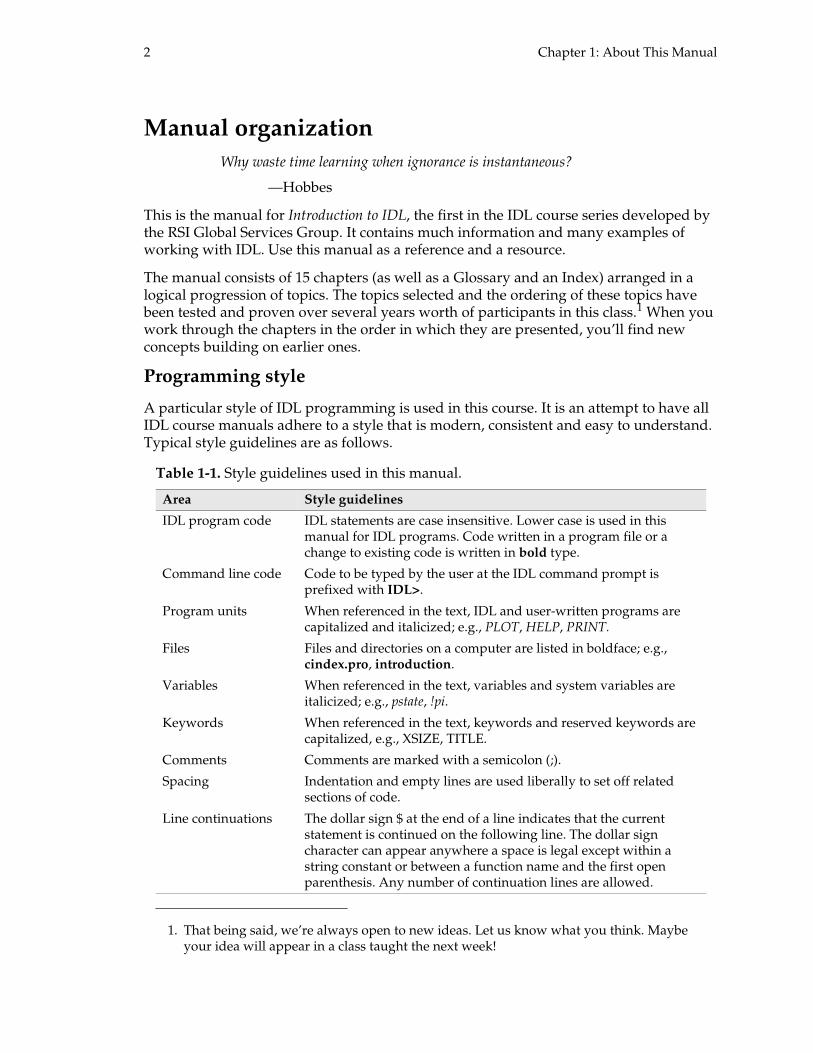
A particular style of IDL programming is used in this course. It is an attempt to have all IDL course manuals adhere to a style that is modern, consistent and easy to understand. Typical style guidelines are as follows.
1. That being said, we’re always open to new ideas. Let us know what you think. Maybe your idea will appear in a class taught the next week!
Table 1-1. Style guidelines used in this manual.
Area Style guidelines
IDL program code IDL statements are case insensitive. Lower case is used in this manual for IDL programs. Code written in a program file or a change to existing code is written in bold type.
Command line code Code to be typed by the user at the IDL command prompt is prefixed with IDL>.
Program units When referenced in the text, IDL and user-written programs are capitalized and italicized; e.g., PLOT, HELP, PRINT.
Files Files and directories on a computer are listed in boldface; e.g., cindex.pro, introduction.
Variables When referenced in the text, variables and system variables are italicized; e.g., pstate, !pi.
Keywords When referenced in the text, keywords and reserved keywords are capitalized, e.g., XSIZE, TITLE.
Comments Comments are marked with a semicolon (;).
Spacing Indentation and empty lines are used liberally to set off related sections of code.
Line continuations The dollar sign $ at the end of a line indicates that the current statement is continued on the following line. The dollar sign character can appear anywhere a space is legal except within a string constant or between a function name and the first open parenthesis. Any number of continuation lines are allowed.
Chapter 1: About This Manual 3
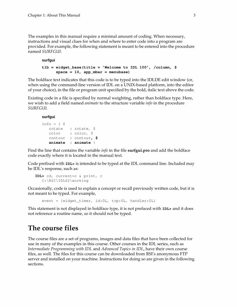
The examples in this manual require a minimal amount of coding. When necessary, instructions and visual clues for when and where to enter code into a program are provided. For example, the following statement is meant to be entered into the procedure named SURFGUI.
surfgui
tlb = widget_base(title = ’Welcome to IDL 100’, /co lumn, $space = 10, app_mbar = menubase)
The boldface text indicates that this code is to be typed into the IDLDE edit window (or, when using the command-line version of IDL on a UNIX-based platform, into the editor of your choice), in the file or program unit specified by the bold, italic text above the code.
Existing code in a file is specified by normal weighting, rather than boldface type. Here, we wish to add a field named animate to the structure variable info in the procedure SURFGUI.
surfgui
info = { $rotate : rotate, $color : color, $contour : contour , $animate : animate }
Find the line that contains the variable info in the file surfgui.pro and add the boldface code exactly where it is located in the manual text.
Code prefixed with IDL> is intended to be typed at the IDL command line. Included may be IDL’s response, such as:
IDL> cd, current=c & print, cC:\RSI\IDL62\working
Occasionally, code is used to explain a concept or recall previously written code, but it is not meant to be typed. For example,
event = {widget_timer, id:0L, top:0L, handler:0L}
This statement is not displayed in boldface type, it is not prefaced with IDL> and it does not reference a routine name, so it should not be typed.
The course files
The course files are a set of programs, images and data files that have been collected for use in many of the examples in this course. Other courses in the IDL series, such as Intermediate Programming with IDL and Advanced Topics in IDL, have their own course files, as well. The files for this course can be downloaded from RSI’s anonymous FTP server and installed on your machine. Instructions for doing so are given in the following sections.

4 Chapter 1: About This Manual
Downloading the course files
RSI’s anonymous FTP site is located at ftp.rsinc.com . There are many OS-specific utilities for performing file transfers; the following description applies to a generic shell-based FTP program available on Windows and UNIX-based operating systems. Note that the anonymous FTP site can also be accessed with a web browser (such as Mozilla) at the URL ftp://ftp.rsinc.com/ .
Type this statement at a UNIX shell prompt or a Windows command prompt:
$ ftp ftp.rsinc.com
Use the word “anonymous” at the name prompt and type your e-mail address as the password (it will not appear on the screen). Your session will look something like this:
$ ftp ftp.rsinc.comConnected to ftp.rsinc.com.220 gateway FTP server ready.
Name (ftp.rsinc.com:mpiper): anonymous331 Guest login ok, send e-mail address as password .Password:[email protected] have connected to Research Systems, Inc.230-230-*********************************************** *******230 Guest login ok, access restrictions apply.Remote system type is UNIX.Using binary mode to transfer files.
Once you have logged on, change directories to /pub/training/IDL_intro and switch to binary mode. Type:
ftp> cd pub/training/IDL_introftp> binary
First, get the README file. It gives background information on the course files.
ftp> get README
Next, download the file that is compatible with your system. For a Windows-based OS, download the zip-compressed file intro.zip:
ftp> get intro.zip
For a UNIX-based OS (i.e., Solaris, Linux, Mac OS X, IRIX, AIX, or HP-UX), download either the tar/gzip or zip version of the course files.
ftp> get intro.tar.gz
End your FTP session with:
ftp> quit
If you are unable to access these files via anonymous ftp, send us an e-mail at [email protected] or call us at 303-786-9900. We will find a way to make the files available to you.

Chapter 1: About This Manual 5
Installing the course files
The following are steps to install the course files on your computer, along with instructions on how to set up IDL to access them. Note that in an RSI class, your instructor will have already performed these steps for you.
1. Select a directory on your computer to install the course files. A suggested location is in the main IDL directory (see “IDL directory structure” on page 20), if it is accessible. Other locations would be under your home directory on a UNIX-based platform or under your My Documents folder on a Windows platform.
2. Use a decompression utility to unpack the course files. For example, on Windows, you can use the shareware package WinZip (www.winzip.com) or the freeware package 7-Zip (www.7-zip.org) . On a UNIX-based platform, use a shell utility such as unzip , gunzip or tar to extract the files.
3. After extraction, the course files will be installed in the directory introduction in the directory IDL_training in the directory you selected for installation. For example, if you installed the files in your My Documents folder on Windows, the directory structure would appear as in the diagram on the right.
This completes the installation of the course files on your machine. Next, we need to instruct IDL where to find them. This involves modifying IDL’s search path settings. More on IDL’s search path can be found in the section “Search path” on page 22.
On Windows:
1. Start IDL. From the Start menu, select Start > Programs > RSI X.X > IDL, or double-click the IDL X.X icon on your desktop; here, X.X is the IDL version number, for example 6.0.
2. In the IDLDE, select File > Preferences from the Menu Bar. This spawns the Preferences dialog. Select the Path tab in the Preferences dialog. Use the controls in this tab to add the directory introduction to IDL’s search path. Click “OK” to finish.
On a UNIX-based platform, including Linux and Mac OS X:
1. Append IDL_training/introduction to the environment variable IDL_PATH. For example, on the c-shell, this is
% setenv IDL_PATH \? {$IDL_PATH}:+{$INSTALL_DIR}/IDL_training/introduc tion
where INSTALL_DIR is the directory in which you installed the course files. Note that the syntax for making an environment variable is shell-dependent.
2. Start IDL, either with the command-line version idl or the development environment idlde .

6 Chapter 1: About This Manual
Chapter relationships
Specific material may be omitted from this course depending upon student interest and previous experience according to the graph in Figure 1-1. The Basics, Variables, Graphics systems, File I/O and Programming chapters are considered particularly valuable for further study of IDL and are strongly suggested.
Figure 1-1. Sequence requirements for covering chapters in this manual.
Contacting RSI Global Services
RSI offers a full range of courses for our products. The courses are designed for beginning IDL users to experienced IDL application developers. We teach courses monthly in Boulder, Colorado and at various regional settings in the United States and around the world. We also teach courses at customers’ sites, as well as courses with customized content.
RSI also offers consulting services. We have years of experience successfully providing custom solutions on time and within budget for a wide range of different organizations with myriad needs and goals.
If you would like more information about our services, or if you have difficulty using this manual or finding the course files, please contact us at:
RSI Global Services4990 Pearl East CircleBoulder, CO 80301 USAPhone: 303-786-9900Fax: 303-786-9909E-Mail: [email protected], [email protected]: http://www.rsinc.com/gsg

7
Chapter 2:
A Tour of IDL
This chapter provides a brief tour of IDL, demonstrating aspects of the language as well as IDL’s built-in visualization capabilities.
Overview . . . . . . . . . . . . . . . . . . . . . . . . . . . . . . . 8Scalars and arrays . . . . . . . . . . . . . . . . . . . . . . . . 8Line plots . . . . . . . . . . . . . . . . . . . . . . . . . . . . . . . 9Surface plots . . . . . . . . . . . . . . . . . . . . . . . . . . . 11Contour plots . . . . . . . . . . . . . . . . . . . . . . . . . . 12
Displaying and processing images . . . . . . . . 13IDL Intelligent Tools (iTools) . . . . . . . . . . . . 14Conclusion . . . . . . . . . . . . . . . . . . . . . . . . . . . . 14Exercises . . . . . . . . . . . . . . . . . . . . . . . . . . . . . . 14Suggested reading . . . . . . . . . . . . . . . . . . . . . 15

8 Chapter 2: A Tour of IDL
Overview
This chapter provides a set of guided exercises to help you get familiar with the basic functionality of IDL. You’re not expected to understand every line of code at this point. The topics covered here will be explained in greater detail as the course progresses.
Please type the statements that are prefaced with the IDL> prompt. A short explanation for each statement or group of statements follows.
Start by calling the JOURNAL procedure. It opens a file to log the statements typed at the command line.
IDL> journal, ’tour.pro’
From this point onward, every statement typed at the command line in the current IDL session is echoed to the file tour.pro. After we finish the tour, you can open this file to view what you typed.
Scalars and arrays
We can use IDL interactively by typing single statements and viewing the results.
IDL> print, 3*412
The PRINT procedure displays the result of the expression 3*4 in IDL’s output log. Note that the comma is used to delimit arguments to an IDL procedure or function.
IDL allows you to make variables on the fly. Let’s look at an example of a scalar variable. (A scalar represents a single value.)
IDL> a = 5*12IDL> help, aA INT = 60
Here, a is a scalar variable. We can get information about a with the HELP procedure. HELP is useful for obtaining diagnostic information from IDL. Notice that in addition to a value, a is associated with a type of number. By default, numbers without decimal points are treated as two-byte integers. Had we instead typed
IDL> a = 5.0*12.0IDL> help, aA FLOAT = 60.0000
the result would be a floating-point value.
Next, let’s look at an example of an array variable. (An array represents multiple values.)
IDL> b = fltarr(10)IDL> help, bB FLOAT = Array[10]IDL> print, b0.000000 0.000000 0.000000 0.000000 0.0000000.000000 0.000000 0.000000 0.000000 0.000000

Chapter 2: A Tour of IDL 9
The FLTARR function is used to create floating-point arrays. Here, the variable b is a 10-element floating point array. By default, the values of b are initially set to zero. Note that the arguments to an IDL function are enclosed in parentheses.
IDL has control statements similar to those in other programming languages. For example, a FOR loop executes a statement, or a group of statements, a specified number of times. Here’s an example of initializing the array b with values. Each element of b receives the value of its array index.
IDL> for i = 0, 9 do b[i] = iIDL> print, b0.00000 1.00000 2.00000 3.00000 4.000005.00000 6.00000 7.00000 8.00000 9.00000
However, in IDL, the built-in function FINDGEN creates an indexed array automatically:
IDL> c = findgen(10)IDL> help, cC FLOAT = Array[10]IDL> print, c0.00000 1.00000 2.00000 3.00000 4.000005.00000 6.00000 7.00000 8.00000 9.00000
In IDL, using built-in array functions is much faster than performing equivalent operations with a control statement.
Arrays are handy because they store groups of numbers or text. We can access individual elements or groups of elements from an array by subscripting the array.
IDL> print, c[0:4]0.000000 1.00000 2.00000 3.00000 4.00000
Here we have extracted a portion of the array c. Notice that array index values start at zero in IDL.
New variables can be made from subscripted arrays.
IDL> d = c[1:6]IDL> help, dD FLOAT = Array[6]
The array d is copied from elements 1 through 6 inclusive of the array c.
Line plots
IDL excels at data visualization. One means of viewing a sequence of data values, like a time series, is to display them as a line plot using the PLOT procedure.
In this example, we’ll read data from a file and display it as a line plot. To simplify the process of reading the data from the file, we’ll use the course program LOAD_DATA. We’ll go into the details of file manipulation in IDL in a subsequent chapter.
Read a set of data values into a new variable chirp. These data represent a sine wave with exponentially increasing frequency.

10 Chapter 2: A Tour of IDL
IDL> chirp = load_data(’chirp’)IDL> help, chirpCHIRP BYTE = Array[512]
The data values are read from a file into IDL in the form of a one-dimensional array (also called a vector). Note the type of the array is byte.
What’s in this variable chirp? With PRINT, we could view the data in tabular form, but considering there are 512 values, the data may be easier to comprehend when viewed graphically. Display the data with the PLOT procedure.
IDL> plot, chirp
A graphics window appears, containing a plot that looks like Figure 2-1.
Figure 2-1. A plot of the ‘chirp’ data.
Plot the data with symbols instead of a line by using the PSYM keyword to PLOT.
IDL> plot, chirp, psym=1
The previous plot is erased and the new plot appears in the same graphics window. Plot with a line and a symbol by using the PSYM and LINESTYLE keywords.
IDL> plot, chirp, psym=-1, linestyle=2
Notice how plots with different characteristics can be created by using keywords to the PLOT procedure. Plot the data and add descriptive titles.
IDL> plot, chirp, xtitle=’Time (s)’, ytitle=’Amplitude ( m)’, $IDL> title=’Sine Wave with Exponentially Increasing Freq uency’
This statement was too long to fit on a single line in the manual. In IDL, a statement can be broken into multiple lines with the continuation character $. When typing at the command line, the statement can be entered in one line and the continuation character can be omitted.

Chapter 2: A Tour of IDL 11
Surface plots
Use LOAD_DATA to read the data ‘lvdem’ into the local variable dem. These data represent elevation values taken from a USGS digital elevation map (DEM) of the Big Thompson Canyon near Loveland, Colorado.
IDL> dem = load_data(’lvdem’)IDL> help, demDEM INT = Array[64, 64]
The variable dem has two dimensions, representing a -element array of data values. We can view data stored in two-dimensional arrays like this one with the SURFACE procedure.
IDL> surface, dem
SURFACE gives a wire mesh representation of the data. The SHADE_SURF procedure provides another means of visualizing these data.
IDL> load_graysIDL> shade_surf, dem
SHADE_SURF displays a filled surface that uses light source shading to give the appearance of depth, with shades provided by the course program LOAD_GRAYS. Try viewing the dem data from a vantage point high above the earth’s surface by rotating the surface using the AX and AZ keywords.
IDL> shade_surf, dem, az=0, ax=90
Experiment with other orientations. As a challenge, try to reproduce the orientation displayed in Figure 2-2 below.
Figure 2-2. The Big Thompson Canyon DEM viewed with SHADE_SURF.
64 64×

12 Chapter 2: A Tour of IDL
Contour plots
Data stored in two-dimensional arrays can also be displayed as a contour plot in IDL.
IDL> contour, dem
By default, the CONTOUR procedure chooses the number of isopleths to plot, as well as the axis values. Override these defaults by using the XSTYLE, YSTYLE and NLEVELS keywords.
IDL> contour, dem, xstyle=1, ystyle=1, nlevels=12
Allowing IDL to choose contour levels is useful for getting a first look a data set, but a better technique is to assign contour levels, given knowledge of the data ranges in each dimension. Start by determining the minimum and maximum values of the data set with the MIN and MAX functions.
IDL> print, min(dem), max(dem)2853 3133
From these values, define a set of contour levels and apply them to the plot through the LEVELS keyword. Use the FOLLOW keyword to display values on the contours. Note that you can use the up arrow on your keyboard to retrieve and edit a command you typed earlier in your IDL session.
IDL> clevels = indgen(15)*25+2800IDL> contour, dem, xstyle=1, ystyle=1, levels=clevels, / follow
Compare your result with Figure 2-3 below.
Figure 2-3. The Big Thompson Canyon DEM viewed with CONTOUR.

Chapter 2: A Tour of IDL 13
Displaying and processing images
IDL can be used to display arrays as images. Data values in an array are matched to grayscale intensities or colors.
Erase the current display window, load a grayscale color palette and display the Big Thompson Canyon DEM as an image using the TVSCL procedure.
IDL> eraseIDL> loadct, 0IDL> tvscl, dem
The resulting image is really small! This is because the elements in the array dem are matched to the pixels of your computer’s display. The array is 64 elements on a side, so the resulting image is 64 pixels on a side. You can use IDL to determine your screen resolution with the GET_SCREEN_SIZE function:
IDL> print, get_screen_size()1280.00 1024.00
Resize dem by interpolation to a -element array using the REBIN function. Store the result in the variable new_dem. Display the result.
IDL> newx = 256IDL> newy = 256IDL> new_dem = rebin(dem, newx, newy)IDL> tvscl, new_dem
Images can be displayed with different color palettes. The image data aren’t altered; rather, the colors used to display them are. Load a predefined color table and display the image using these colors in a window with the same dimensions as the image.
IDL> loadct, 5IDL> window, 0, xsize=newx, ysize=newyIDL> tvscl, new_dem
Compare your results with Figure 2-4 below.
Figure 2-4. The Big Thompson Canyon DEM viewed with TVSCL.
256 256×

14 Chapter 2: A Tour of IDL
Since the data used to display this image are just numbers, IDL can crunch them. Try differentiating the image using the SOBEL function. SOBEL is often used as an edge enhancer.
IDL> tvscl, sobel(new_dem)
In the processed image, the canyon walls have high pixel values—orange and red in this color table—because these regions of steep elevation change must have a derivative that is larger than zero in magnitude. On the other hand, the canyon floor has low pixel values—blue and black—because it’s flatter, implying a smaller derivative.
IDL Intelligent Tools (iTools)
The IDL Intelligent Tools (iTools), introduced in IDL 6.0, provide new means of interactively visualizing data, with a programmatic and point-and-click interface.
Look at the Big Thompson Canyon DEM with an iSurface tool.
IDL> isurface, dem
A splash screen appears while the iTools load. Once loading is complete, the Big Thompson Canyon data is displayed as a shaded surface. You can use the mouse to pan the graphic. By accessing the buttons on the Tool Bar, you can also rotate and scale the graphics. Try changing the default color of the surface or the font size on the axes. Add some annotation. Export the graphics to a JPEG file. As a challenge, try to reproduce the positioning and annotation of the data displayed in Figure 2-5 on page 15.
When finished, clean up the iTools using the ITRESET procedure.
IDL> itreset
Further use of the iTools is presented in Chapter 5, “IDL iTools.” You can also refer to the iTool User’s Guide for more information.
Conclusion
End the tour with a second call to the JOURNAL procedure.
IDL> journal
This statement turns off journalling. Open the file tour.pro to see what you’ve typed!
Exercises
1. Try using CONTOUR’s FILL keyword to display a filled contour plot.
2. Use the IMAGE_CONT procedure to display the Big Thompson Canyon DEM as an image with contours.
3. Use the Surface-Contour button on the Tool bar to draw contours over the data displayed in the iTool in Figure 2-5.

Chapter 2: A Tour of IDL 15
Figure 2-5. The Big Thompson Canyon data set viewed with an IDL iTool.
Suggested reading
Fanning, David F. IDL Programming Techniques. Second Edition. Fort Collins, Colorado: Fanning Software Consulting, 2000.
A useful introductory book written by an original member of the Training Department at RSI. Dr. Fanning excels at explaining the idiosyncrasies of IDL to new and experienced users.
Research Systems. Getting Started with IDL. Boulder, Colorado: Research Systems, 2005.
This document gives many tutorial-like examples of using IDL that are suitable for new users. From the Contents tab of the IDL Online Help utility, select User’s Guides > Getting Started with IDL.

16 Chapter 2: A Tour of IDL
Research Systems. iTool User’s Guide. Boulder, Colorado: Research Systems, 2005.
An explanation of how to use the new IDL iTools, along with many examples. This document can be accessed in the same manner as Getting Started with IDL, described above.

17
Chapter 3:
IDL Basics
Some of the basics of using IDL are presented in this chapter.
The IDL Development Environment . . . . . . . 18 IDLDE shortcuts and tips . . . . . . . . . . . . . . . 19 Notes on UNIX-based platforms . . . . . . . . . 20IDL directory structure . . . . . . . . . . . . . . . . . . 20 Search path . . . . . . . . . . . . . . . . . . . . . . . . . . . 22IDL Online Help . . . . . . . . . . . . . . . . . . . . . . . . 23Statements and programs . . . . . . . . . . . . . . . . 23
Executive commands . . . . . . . . . . . . . . . . . . 24 Main . . . . . . . . . . . . . . . . . . . . . . . . . . . . . . . . 25 Procedure . . . . . . . . . . . . . . . . . . . . . . . . . . . . 25 Function . . . . . . . . . . . . . . . . . . . . . . . . . . . . . 26 Positional and keyword parameters . . . . . 26Batch files . . . . . . . . . . . . . . . . . . . . . . . . . . . . . 27Suggested reading . . . . . . . . . . . . . . . . . . . . . 27

18 Chapter 3: IDL Basics
The IDL Development Environment
...the command line continued to exist as an underlying stratum—a sort of brainstem reflex—of many computer systems.
—Neal Stephenson, In the Beginning was the Command Line
The IDL Development Environment (IDLDE) is a graphical user interface that provides built-in editing and debugging tools for IDL. Figure 3-1 shows an annotated screenshot of the IDLDE for Windows. (UNIX-based platforms—e.g., Solaris, Linux, MacOS X—have an IDLDE that is similar in appearance, built with the Motif toolkit.)
Figure 3-1. The IDL Development Environment (MS Windows).
A summary of the functionality of the components of the IDLDE is given in Table 3-1.
Table 3-1. IDLDE components.
IDLDE component Function
Menu bar Controls for opening, editing, compiling and running IDL programs, as well as other features of the IDLDE.
Tool bar Graphical controls with functionality similar to that of the Menu bar.
Project window A tool for convenient grouping of IDL programs and data files.
Editor window Where IDL programs are written and edited.
Output log Used by IDL to return information to the user; also used to echo statements entered at the command prompt.
menu bar
tool bar
project window
editor window
output log
variable watch window
commandprompt
status bar
menu bar
tool bar
project window
editor window
output log
variable watch window
commandprompt
status bar
Chapter 3: IDL Basics 19
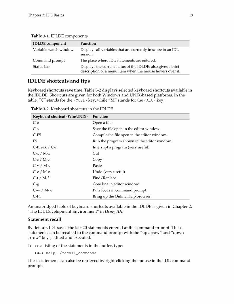
IDLDE shortcuts and tips
Keyboard shortcuts save time. Table 3-2 displays selected keyboard shortcuts available in the IDLDE. Shortcuts are given for both Windows and UNIX-based platforms. In the table, “C” stands for the <Ctrl> key, while “M” stands for the <Alt> key.
An unabridged table of keyboard shortcuts available in the IDLDE is given in Chapter 2, “The IDL Development Environment” in Using IDL.
Statement recall
By default, IDL saves the last 20 statements entered at the command prompt. These statements can be recalled to the command prompt with the “up arrow” and “down arrow” keys, edited and executed.
To see a listing of the statements in the buffer, type:
IDL> help, /recall_commands
These statements can also be retrieved by right-clicking the mouse in the IDL command prompt.
Variable watch window Displays all variables that are currently in scope in an IDL session.
Command prompt The place where IDL statements are entered.
Status bar Displays the current status of the IDLDE; also gives a brief description of a menu item when the mouse hovers over it.
Table 3-2. Keyboard shortcuts in the IDLDE.
Keyboard shortcut (Win/UNIX) Function
C-o Open a file.
C-s Save the file open in the editor window.
C-F5 Compile the file open in the editor window.
F5 Run the program shown in the editor window.
C-Break / C-c Interrupt a program (very useful)
C-x / M-x Cut
C-c / M-c Copy
C-v / M-v Paste
C-z / M-z Undo (very useful)
C-f / M-f Find/Replace
C-g Goto line in editor window
C-w / M-w Puts focus in command prompt.
C-F1 Bring up the Online Help browser.
Table 3-1. IDLDE components.
IDLDE component Function

20 Chapter 3: IDL Basics
Startup file
A startup file contains commands that are executed when a new IDL session is started. A startup file can be used to set up colors, define useful system variables or compile library files. A startup file is a batch file, not a program. More information on batch files is given in the section “Batch files” below.
The startup file location can be set in the Startup tab in the IDLDE Preferences... dialog. Alternately, on a UNIX-based platform you can set the environment variable $IDL_STARTUP to designate the location of the startup file.
Session logging
Statements entered at the IDL command line can be logged in a file using the JOURNAL procedure. Journaling was used, for example, in Chapter 2, “A Tour of IDL.” JOURNAL is called with one argument, the name of the journal file. For example,
IDL> journal, ’idl_journal.pro’
Creating a journal file overwrites any file with the same name. The previous contents of that file are lost. Exercise caution when supplying a filename argument to JOURNAL.
The system variable !journal stores the current state of journalling; it is 0 when journalling is off, 1 when it is on.
Turn off journalling by calling JOURNAL without an argument.
IDL> journal
Notes on UNIX-based platforms
On a UNIX-based platform, the IDLDE can be launched by typing
$ idlde
at a shell prompt. A command-line version of IDL can be started with
$ idl
With the command-line version, you can use your favorite editor to create and edit IDL programs. Some editors, such as vim, (X)Emacs, NEdit and jEdit, have built-in color syntaxing for IDL. (X)Emacs has a built-in major mode, IDLWAVE, which is particularly powerful; in addition to syntax highlighting, it allows command completion, autoindenting, and expandable command abbreviations. See idlwave.org for more information.
IDL directory structure
By default, IDL is installed in a particular location on Windows and UNIX-based platforms.
• Windows (2000, XP): C:\RSI\IDLXX, where XX is the IDL version number; 6.2, for example.

Chapter 3: IDL Basics 21
• UNIX-based (e.g, Solaris, Linux, Mac OS X): /usr/local/rsi/idl_X.X, where X.X is the IDL version number. The environment variable $IDL_DIR contains the path to this directory.
This installation directory is called the main IDL directory. It is used as a reference point for locating other files in the IDL distribution. Within IDL, the !dir system variable stores the path to this directory. (System variables are discussed in Chapter 7, “Variables.”)
As Figure 3-2 shows, the directories under the main IDL directory are the same on Windows and UNIX-based platforms. A list of the directories and an overview of their contents are given in Table 3-3.
With a common directory structure, if you know the location of a file under the main IDL directory on one system running IDL, you’ll know its location on another system, even if it’s on another platform. The FILEPATH function can be used to specify an absolute path to a file located relative to the main IDL directory. For example, if you wished to use the file help3.bmp in a program, you can specify its location by typing
IDL> filename = filepath(’help3.bmp’, subdir=[’resource’ ,’bitmaps’])
On Windows, printing the variable filename results in
C:\RSI\IDL62\resource\bitmaps\help3.bmp
whereas on a UNIX-based system, it is
/usr/local/rsi/idl_6.2/resource/bitmaps/help3.bmp
Figure 3-2. IDL’s directory structure on Linux and Windows.

22 Chapter 3: IDL Basics
Search path
The search path is an ordered list of directories that IDL searches to find program, batch and save files. Using a path is efficient: rather than looking through the entire directory tree, only a smaller subset of directories are searched where IDL might expect to find files.
The concept of path is used in operating systems. Both Windows and UNIX-based operating systems have a PATH environment variable, or some variant of it. The path is used to tell the operating system where to find executables, like iexplore in Windows or ls in UNIX. Instead of searching the entire file system for executables, only directories in the path are searched.
The IDL search path is stored as a string in the system variable !path. (System variables are covered in Chapter 7, “Variables”). Manually editing the !path system variable is possible, but tedious. The IDLDE provides a convenient graphical interface for manipulating the path in the Path tab of the Preferences dialog. An example of this dialog is shown in Figure 3-3. By default, one entry, <IDL_DEFAULT>, exists; it points to the lib and examples subdirectories of the IDL distribution. Other directories can added, subtracted and positioned using the Insert, Remove and arrow buttons. Note that IDL searches directories in the order that they are listed in the path. If an IDL file exists outside of the path, IDL will not automatically find it; its location will need to be explicitly specified.
On UNIX-based platforms, the environment variable $IDL_PATH can be used to set IDL’s path. Note that the path settings in the IDLDE Preferences dialog will be overridden by $IDL_PATH. After starting IDL, the Preferences can be used to modify the settings in the !path system variable in the current session.
Table 3-3. The directories in the IDL distribution.
Name Contents
bin Stores the IDL executable, as well as shared objects that are loaded dynamically into IDL.
examples Stores example program files, data sets and images.
external Contains information and examples of linking IDL with code written other languages, such as Fortran, C, java and Visual Basic.
help The location of the IDL Online Help browser files, in PDF format.
lib The storage location for the IDL routines that are a part of the distribution, but are written in the IDL language itself.
products The location where other RSI products, such as ENVI, are stored.
resource A catch-all directory that contains fonts IDL uses, the IDL mapping databases, as well as bitmap buttons for building the IDLDE.

Chapter 3: IDL Basics 23
Figure 3-3. An example of the Windows IDLDE Preferences, displaying path settings.
IDL Online Help
IDL is equipped with an extensive documentation system, IDL Online Help. With Online Help, you can learn about routines and their inputs, as well as a great deal of general IDL information.
Start the Online Help browser by typing a question mark at the IDL command prompt
IDL> ?
or by selecting Help > Contents... from the IDLDE menu bar. On UNIX-based systems, the Online Help browser can also be started from a shell prompt:
$ idlhelp
Online Help provides detailed documentation for every IDL routine. Starting with IDL 6.2, the Online Help also contains the entire IDL documentation set from RSI.
Statements and programs
A statement is an instruction that tells a computer what to do. Statements are the syntactic equivalent of complete sentences — they express complete thoughts. They are the programmer’s unit of communication with IDL. IDL statements are case insensitive, with the only exception being characters inside a string.
A program is a sequence of statements that act as a unit. IDL supports three program types: main, procedure and function. Procedures and functions are keys to structured modular programming, a proven programming philosophy. We encourage you to write procedures and functions instead of main programs.

24 Chapter 3: IDL Basics
All programs must be compiled before they can be executed. Compiling is the act of interpreting the source code statements from a file and converting them into an intermediate bytecode stored in memory. This bytecode is what is executed when you run the program.
Executive commands
Executive commands are the statements used to compile, run, stop, and step through IDL procedures, functions and main programs. Executive commands always begin with a period. They may only be called from the command prompt or in IDL’s noninteractive batch mode.Table 3-4 gives a list of executive commands.
An executive command may be abbreviated to the smallest number of characters that uniquely identify it. For example, .comp can be substituted for .compile .
Table 3-4. Executive commands.
Command Description
.compile filename Compiles program modules
.continue Continues execution of a program that has been stopped because of an error, a STOP statement, or a keyboard interrupt
.edit filename Opens files in IDLDE editor windows
.full_reset_session Extends .reset_session by removing all system routines and libraries external to the IDL distribution
.go Executes a previously compiled main program
.out Continues program execution until the current program module returns to its caller
.reset_session Resets IDL system memory, removing variables, compiled user functions and procedures
.return Continues execution until a RETURN statement is encountered
.run filename Compiles IDL procedures, functions and main programs, executes main programs; if called without a filename, it can be used to compose, compile, and run a main-level program from the command prompt
.rnew filename Similar to .run , except that all user variables are erased before the new main program is executed
.skip n Skips over the specified number of statements in the current program; n = 0, 1, 2,...
.step n Executes a specified number of statements in the current program, then stops; n = 0, 1, 2,...
.stepover Steps over calls to other program units
.trace Similar to .continue , but it displays each line of code before it executes it

Chapter 3: IDL Basics 25
The Run menu in the IDLDE menu bar also contains entries that match these executive commands. In the IDLDE, you have the option of using the menu bar items or typing the executive commands directly at the command prompt.
Main
A main program consists of a sequence of IDL statements terminated with an END statement. Only one main program can exist in an IDL session at any time.
An example of a main program is shown on the right. This main program exists in the file hello.pro in the introduction directory.
Compile and execute this main program with the .run executive command:
IDL> .run helloHello World
One side effect of running a main program is that any variables defined in the program reside in IDL’s memory after the program ends. Running several main programs in a series could, for example, cause IDL to allocate more memory for a session than is necessary.
Procedure
A procedure is a self-contained IDL program; i.e., any variable defined in a procedure is deleted when the program ends, unless it is passed out through a parameter. A procedure starts with the procedure declaration statement, consisting of the reserved keyword PRO, the name of the procedure, and any parameters for the procedure. The body of the procedure follows. A procedure is terminated with an END statement.
An example of a procedure is shown on the right. This procedure exists in the file pwd.pro in the introduction directory.
Compile the procedure by issuing the .compile executive command:
IDL> .compile pwd
Execute the procedure by calling it by name:
IDL> pwdC:\RSI\IDL62\working
If the file containing this procedure had not been in IDL’s search path, it could still be compiled by specifying its file path in the .compile statement. For example, if pwd.pro had been stored in the directory C:\temp, which is not in the IDL path, the .compile statement would be
IDL> .compile "C:\temp\pwd.pro"
IDL would locate the file and compile its contents. The procedure could then be executed by calling it by name, as before.
hello.pro
print, ’Hello World’end
pwd.pro
pro pwd cd, current=c print, cend

26 Chapter 3: IDL Basics
Function
A function is another self-contained IDL program, like a procedure; however, a function typically returns information to its caller. A function begins with the function declaration statement, consisting of the reserved keyword FUNCTION, the name of the function, and any parameters for the function. The body of the function, which usually includes at least one RETURN statement, follows. A function is terminated with an END statement.
The example function on the right exists in the file is_positive.pro in the introduction directory.
Compile the function by issuing the .compile executive command:
IDL> .compile is_positive
The syntax for calling this function is:
IDL> x = is_positive(5)IDL> print, x
1
As with the procedure, if the file containing this function had not been in IDL’s search path, it could still be compiled by specifying its absolute file path in the .compile statement.
Positional and keyword parameters
Parameters are used to pass information between programs. IDL has two types of parameters: positional and keyword. Though either type can be used to send or receive information, positional parameters are typically used for required information, whereas keywords are used for optional information. How parameters are employed, though, is a programmer’s choice. The type and ordering of parameters for built-in IDL routines can be determined by looking up the routine in the IDL Online Help.
The ordering of positional parameters in a call to a program is important. For example, if x and y are vectors, say
IDL> x = findgen(20)IDL> y = x^2
then this PLOT statement
IDL> plot, x, y
is different than this one
IDL> plot, y, x
Keyword parameters, on the other hand, can be listed in any order. For example, the following statements produce the same result:
IDL> plot, x, y, xtitle=’Time’, ytitle=’Speed’IDL> plot, x, y, ytitle=’Speed’, xtitle=’Time’
is_positive.pro
function is_positive, x return, x gt 0end

Chapter 3: IDL Basics 27
Keyword parameters can be abbreviated. This is useful when using IDL interactively at the command prompt, but it is not recommended when programming, since it may confuse a reader.
Certain keywords are either "on" or "off", with "off" the default. Such keywords may be set (turned "on") with the forward slash "/". For example, the following statements produce the same result:
IDL> plot, x, y, /nodataIDL> plot, x, y, nodata=1
The "slash" keyword syntax is commonly used by IDL programmers. Though it is a handy visual clue that a keyword is being set, it saves all of one keystroke.
Batch files
A batch file is a sequence of individual IDL statements. A batch file is not a program — it cannot be compiled. Rather, each statement in the file is interpreted and executed sequentially by IDL.
The example on the right, stored in the file batch_ex.pro in the introduction directory, could be used as an example of a startup file. To execute this batch file, type:
IDL> @batch_exWed Oct 19 11:27:07 2005C:\RSI\IDL62
Had batch_ex.pro not been in IDL’s path, a quoted absolute or relative filepath could be specified after the @ symbol.
On a UNIX-based system, IDL’s batch mode can be a powerful tool. For example, a command like the following can be executed from the shell:
$ idl < batch_ex.pro > batch.out &
With this command, IDL starts and runs in the background. It accepts a sequence of commands from the file batch_ex.pro and redirects the output to the file batch.out. When finished, IDL exits.
Suggested reading
Fanning, David F. IDL Programming Techniques. Second Edition. Fort Collins, Colorado: Fanning Software Consulting, 2000.
A useful introductory book written by the founder of the Training Department at RSI. Dr. Fanning excels at explaining the idiosyncrasies of IDL.
batch_ex.pro
print, systime()pwd

28 Chapter 3: IDL Basics
Gumley, Liam E. Practical IDL Programming. San Francisco: Morgan Kaufmann, 2001.
An excellent book on general IDL programming recommended by David Stern, creator of IDL and founder of RSI.
Research Systems. Using IDL. Boulder, Colorado: Research Systems, 2005.
Chapter 2 of this document describes the components of the IDLDE. From the Contents tab of the Online Help browser, select User’s Guides > Using IDL.

29
Chapter 4:
Graphics Systems
The two graphics systems in IDL, Direct Graphics and Object Graphics, are compared and contrasted. Basics of Direct Graphics use such as dealing with graphics windows and specifying colors are described in detail. Tips for working with systems with 8-bit color are discussed.
Direct Graphics vs. Object Graphics . . . . . . . 30Graphics windows in Direct Graphics . . . . . 30Color in Direct Graphics . . . . . . . . . . . . . . . . . 33 Decomposed color . . . . . . . . . . . . . . . . . . . . . 33
Indexed color . . . . . . . . . . . . . . . . . . . . . . . . . 34 8-bit color . . . . . . . . . . . . . . . . . . . . . . . . . . . . 36Exercises . . . . . . . . . . . . . . . . . . . . . . . . . . . . . . 38Suggested reading . . . . . . . . . . . . . . . . . . . . . 38

30 Chapter 4: Graphics Systems
Direct Graphics vs. Object Graphics
From there to here,from here to there,funny thingsare everywhere.
—Dr. Seuss, One fish two fish red fish blue fish.
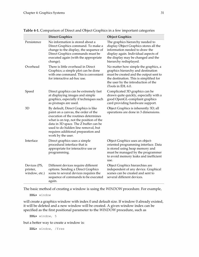
IDL has two completely separate graphics systems: Direct Graphics and Object Graphics. Although Object Graphics is more modern, Direct Graphics is by no means obsolete. Each system has its own advantages and disadvantages. These are summarized in the Table 4-1.
The basic axiom to remember about the differences between the systems is: Direct Graphics makes simple things easy, Object Graphics makes complicated things possible.
Direct Graphics will be discussed in more detail in the rest of the chapter. See the Intermediate Programming with IDL course for more information about Object Graphics.
The command
IDL> help, /deviceAvailable Graphics Devices: CGM HP METAFILE NULL PC L PRINTER PS WIN ZCurrent graphics device: WIN Screen Resolution: 1280x1024 Simultaneously displayable colors: 16777216 Number of allowed color values: 16777216 System colors reserved by Windows: 0 IDL Color Table Entries: 256 NOTE: this is a TrueColor device Using Decomposed color Graphics Function: 3 (copy) Current Font: System,Current TrueType Font: <de fault> Default Backing Store: None.
reports the capabilities and status of the current graphics device to the output log. Note that these capabilities are requested from the operating system, not directly from the hardware—you may need to set the preferences in the operating system to make use of the full capabilities of the hardware.
Graphics windows in Direct Graphics
It is possible to have many Direct Graphics windows open and available for output. Each window has a graphics window index by which that window is referred. The current graphics window’s index is stored in the system variable !d.window . All Direct Graphics output goes to the current graphics window. If there is no current graphics window (there are no graphics windows open), then !d.window will be -1. If a command is issued to output Direct Graphics when there is no current graphics window, a new window will be created and that will become the current graphics window.
Chapter 4: Graphics Systems 31
The basic method of creating a window is using the WINDOW procedure. For example,
IDL> window
will create a graphics window with index 0 and default size. If window 0 already existed, it will be deleted and a new window will be created. A given window index can be specified as the first positional parameter to the WINDOW procedure, such as
IDL> window, 5
but a better way to create a window is:
IDL> window, /free
Table 4-1. Comparison of Direct and Object Graphics in a few important categories
Direct Graphics Object Graphics
Persistence No information is stored about a Direct Graphics command. To make a change to the display, the sequence of Direct Graphics commands must be executed again (with the appropriate change).
The graphics hierarchy needed to display Object Graphics stores all the information needed to draw the display again. Individual aspects of the display may be changed and the hierarchy redisplayed.
Overhead There is little overhead in Direct Graphics; a simple plot can be done with one command. This is convenient for interactive ad-hoc use.
No matter how simple the graphics, a graphics hierarchy and destination must be created and the output sent to the destination. This is simplified for the user by the introduction of the iTools in IDL 6.0.
Speed Direct graphics can be extremely fast at displaying images and simple graphics, especially if techniques such as pixmaps are used.
Complicated 3D graphics can be drawn quite quickly, especially with a good OpenGL-compliant graphics card providing hardware support.
3D By default, Direct Graphics is like paint on a canvas, the order of the execution of the routines determines what is on top, not the position of the data in 3D space. The Z buffer can be used to do hidden line removal, but requires additional preparation and work by the user.
Object Graphics is inherently 3D; all operations are done in 3 dimensions.
Interface Direct graphics uses a simple procedural interface that is appropriate for interactive use or programming.
Object Graphics uses an object-oriented programming interface. Data is stored using heap memory and must be managed by the programmer to avoid memory leaks and inefficient use.
Devices (PS, printer, window, etc.)
Different devices require different options. Sending a Direct Graphics scene to several devices requires the sequence of commands to be executed again.
Object Graphics hierarchies are independent of any device. Graphical scenes can be created and sent to several different devices.
32 Chapter 4: Graphics Systems
IDL> print, !d.window
This will create a window with an index that is not currently being used. Remember, !d.window contains the index of the current graphics window which in our case is the new window.
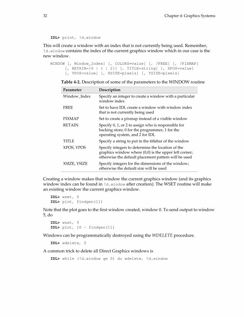
WINDOW [, Window_Index] [, COLORS=value] [, /FREE] [, /PIXMAP][, RETAIN={0 | 1 | 2}] [, TITLE=string] [, XPOS=val ue][, YPOS=value] [, XSIZE=pixels] [, YSIZE=pixels]
Creating a window makes that window the current graphics window (and its graphics window index can be found in !d.window after creation). The WSET routine will make an existing window the current graphics window.
IDL> wset, 0IDL> plot, findgen(11)
Note that the plot goes to the first window created, window 0. To send output to window 5, do
IDL> wset, 5IDL> plot, 10 - findgen(11)
Windows can be programmatically destroyed using the WDELETE procedure.
IDL> wdelete, 0
A common trick to delete all Direct Graphics windows is
IDL> while (!d.window ge 0) do wdelete, !d.window
Table 4-2. Description of some of the parameters to the WINDOW routine
Parameter Description
Window_Index Specify an integer to create a window with a particular window index
FREE Set to have IDL create a window with window index that is not currently being used
PIXMAP Set to create a pixmap instead of a visible window
RETAIN Specify 0, 1, or 2 to assign who is responsible for backing store; 0 for the programmer, 1 for the operating system, and 2 for IDL
TITLE Specify a string to put in the titlebar of the window
XPOS, YPOS Specify integers to determine the location of the graphics window where (0,0) is the upper left corner; otherwise the default placement pattern will be used
XSIZE, YSIZE Specify integers for the dimensions of the window; otherwise the default size will be used

Chapter 4: Graphics Systems 33
Color in Direct Graphics
Colors on computers are created by combining intensities of red, green, and blue channels. Each channel can have a value of 0 (no intensity for that channel) through 255 (full intensity). A color consists of the combined intensities of the three channels, so colors can be expressed as an RGB triple. For example, a pure red color would consist of a full intensity red channel and no intensity green and blue channels. This would be denoted as [255, 0, 0] .
The number of colors displayed by a computer is determined by the graphics display hardware. This is usually referenced by the number of bits per pixel that can be stored, such as 8, 16, or 24 bits. Since the values of 0 to 255 require 8 bits to store and there are three channels to reference a color, 24 bits are needed to fully determine a color. Since a full color cannot be stored, for example, in the 8 bits allocated for each pixel on some systems, there is an indirect method of specifying colors that is used on such systems and can be used on the other systems as well. This is called indexed color and uses a color table to determine which colors are displayed.
Decomposed color
To enter decomposed color mode, type
IDL> device, decomposed=1
Use help, /device to check that IDL is using decomposed color mode.
In decomposed color, all colors are specified directly when needed. In our examples, we will use the ERASE command which simply paints the current graphics window the color specified by its first argument. For example,
IDL> erase, 0L
should paint the current graphics window black. Other graphics commands have other parameters and uses for colors, but all except the same values for a color. To display the color [200, 100, 50], try
IDL> erase, 200 + 100 * 2L^8 + 50 * 2L^16
Figure 4-1. Representation of the a color in decomposed color mode.
If you are familiar with hexadecimal notation, it may be convenient to specify colors like
IDL> erase, ’3264C8’x
which produces the same color since 20010 = C816, 10010 = 6416, and 5010 = 3216. Lastly, there is a course routine provided, RGB2IDX, which makes this conversion more convenient:
IDL> erase, rgb2idx([200, 100, 50])
34 Chapter 4: Graphics Systems
Indexed color
To enter indexed color mode, type
IDL> device, decomposed=0
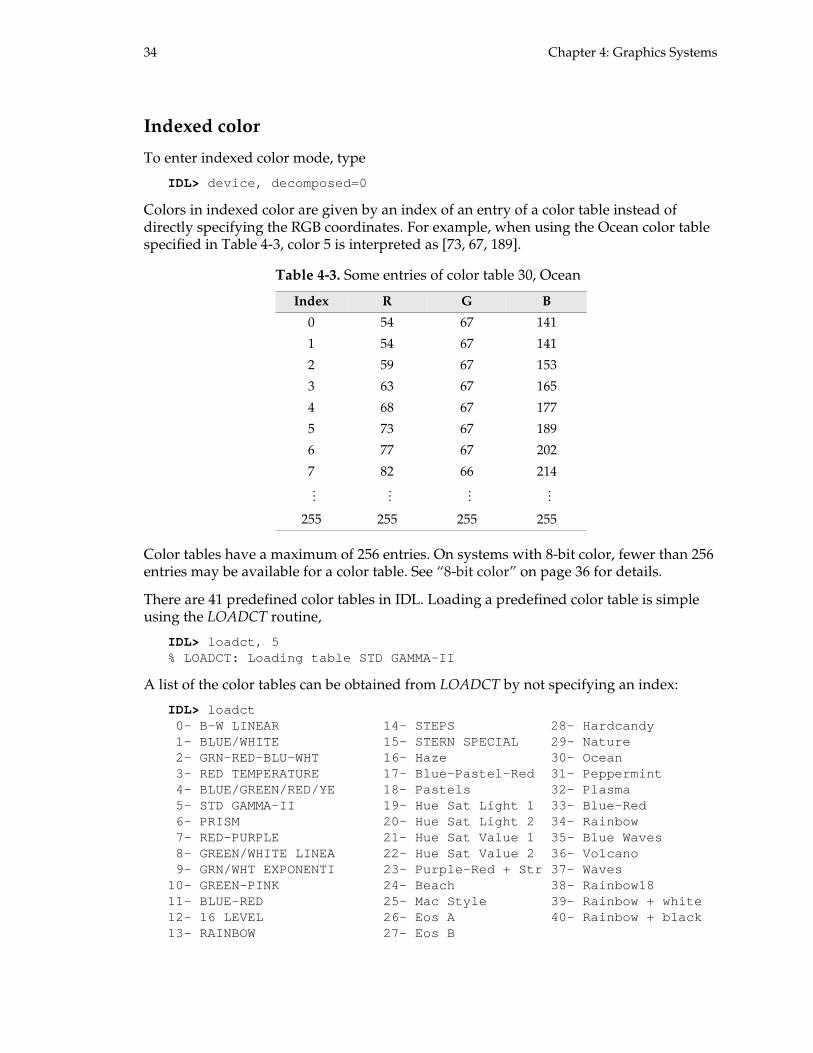
Colors in indexed color are given by an index of an entry of a color table instead of directly specifying the RGB coordinates. For example, when using the Ocean color table specified in Table 4-3, color 5 is interpreted as [73, 67, 189].
Color tables have a maximum of 256 entries. On systems with 8-bit color, fewer than 256 entries may be available for a color table. See “8-bit color” on page 36 for details.
There are 41 predefined color tables in IDL. Loading a predefined color table is simple using the LOADCT routine,
IDL> loadct, 5% LOADCT: Loading table STD GAMMA-II
A list of the color tables can be obtained from LOADCT by not specifying an index:
IDL> loadct0- B-W LINEAR 14- STEPS 28- Hardcandy
1- BLUE/WHITE 15- STERN SPECIAL 29- Nature 2- GRN-RED-BLU-WHT 16- Haze 30- Ocean 3- RED TEMPERATURE 17- Blue-Pastel-Red 31- Peppermin t 4- BLUE/GREEN/RED/YE 18- Pastels 32- Plasma 5- STD GAMMA-II 19- Hue Sat Light 1 33- Blue-Red 6- PRISM 20- Hue Sat Light 2 34- Rainbow 7- RED-PURPLE 21- Hue Sat Value 1 35- Blue Waves 8- GREEN/WHITE LINEA 22- Hue Sat Value 2 36- Volcano 9- GRN/WHT EXPONENTI 23- Purple-Red + Str 37- Waves10- GREEN-PINK 24- Beach 38- Rainbow1811- BLUE-RED 25- Mac Style 39- Rainbow + white12- 16 LEVEL 26- Eos A 40- Rainbow + black13- RAINBOW 27- Eos B
Table 4-3. Some entries of color table 30, Ocean
Index R G B
0 54 67 141
1 54 67 141
2 59 67 153
3 63 67 165
4 68 67 177
5 73 67 189
6 77 67 202
7 82 66 214
… … … …
255 255 255 255

Chapter 4: Graphics Systems 35
Note that the prompt has changed to "Enter table number:" and IDL is waiting for a response. Enter a number 0–40 to load the corresponding color table.
The XLOADCT program is a GUI interface for the same functionality as LOADCT. The predefined color tables can be loaded and manipulated in a few basic ways. Also useful when dealing with color tables is XPALETTE, which gives a better visualization of the individual colors in a color table.
Arbitrary color tables can also be loaded and retrieved with TVLCT routine. For example,
IDL> tvlct, r, g, b, /get
will retrieve the current color table and place the columns into the vectors r, g, and b. To load color table information into the graphics system from vector arrays, simply do not use the GET keyword. For example,
IDL> r = bindgen(256)IDL> g = bytarr(256)IDL> b = 255 - bindgen(256)IDL> tvlct, r, g, b
Use XLOADCT or XPALETTE to view the result.
Figure 4-2. XLOADCT allows a user to interactively load and manipulate color tables.

36 Chapter 4: Graphics Systems
The predefined color tables can be replaced with other color table files. See the online help for the MODIFYCT routine for details on how to create and modify the files that hold the color tables.
8-bit color
On all systems that run IDL there are color limitations when operating in 8-bit mode. These color limitations are caused by windowing systems themselves. The major limitation is the number of colors available to IDL for graphics. On an 8-bit system, there are only 256 available color slots on the graphics card. These colors must be shared by all applications running within the windowing system, including IDL.
The number of colors available to IDL directly affects the size of the color lookup table. IDL maintains a system variable, !d.table_size , that contains the number of colors in the color-lookup table.
IDL> print, !d.table_size
On systems running in 24-bit mode this is always 256. On 8-bit systems the values vary. Note that 24-bit mode and 8-bit mode are not the same as decomposed color and indexed color; they refer to the ability to run in decomposed color.
Windows. Windows uses a system of color sharing between applications. Each operating system takes a certain number of colors from the 256 available and lets all other applications share the rest. Microsoft Windows takes 20 colors and leaves 236 for all other applications. The color lookup table size (!d.table_size) on an 8-bit MS Windows PC is always 236.
UNIX and Mac OS (X Windows). The X Window System that runs on UNIX and VMS machines uses a color allocation scheme with color “cells.” When an X Windows session begins, there are 256 color cells available. Each running application checks out a certain number of cells. When IDL starts, a query of the available color cells is made to X Windows. IDL checks out all of the available color cells. Typical color table sizes range from as high as 220 colors to as low as 50. An example X Window color allocation is laid out in Table 4-4 below.
In this session, the number of colors available to IDL is 161.
Color flashing. One problem that occurs on X Windows is color flashing. The symptom of this is flashing colors on the screen whenever the mouse is moved from window to window. When there are less than a critical number of colors available, IDL creates a private color map with 256 colors. The side effect of private maps is color flashing. This
Table 4-4. Possible X Windows session color usage.
Colors at system startup 256
CDE desktop -50
xterm -20
clock -10
xload -15
Total remaining colors 161

Chapter 4: Graphics Systems 37
occurs because the windows in which IDL runs in steal all the colors from the other applications while those windows are highlighted. The most common cause of a private color map is running two sessions of IDL at the same time or running a color intensive application such as web browser before IDL.
The color lookup table. In 8-bit color mode, the color lookup table can never contain 256 colors, due to the limitations outlined above. When a built-in color table is loaded with either LOADCT or XLOADCT, the 256 colors in the table are scaled into the number of colors available in the system (!d.table_size ). A side effect of this is that on an 8-bit UNIX system, a color index with a certain color table loaded may not contain exactly the same color from day to day. Another side effect is that the only usable color index values are from 0 to !d.table_size-1 . The index values from !d.table_size to 255 contain the same RGB value as the last available index (!d.table_size-1 ).
Programming in 8-bit color. The 8-bit color limitations can be dealt with on a programmatic level. The key is to limit your applications to only the number of colors specified by !d.table_size .
PLOT, CONTOUR and SURFACE. In most cases, the PLOT, CONTOUR and SURFACE routines require several unique colors: background, foreground and annotation colors. One way to approach these types of plots is to create a custom color table loaded in the lower indices. When the color limitation cuts off the upper end of the color table, the custom color table at the bottom is not affected.
Displaying Images with TV and TVSCL. There are several approaches to rendering images on a color limited system. The easiest method is to use the TVSCL procedure. TVSCL looks at the size of the color table and scales the image data into that range before displaying. This method is great when using one of IDL’s built-in color tables. The built-in color tables are automatically scaled to the color lookup table size when loaded with LOADCT. If a custom color table is loaded for an image, it is the user’s responsibility to scale the color table into the range of available colors. This is easily done with the BYTSCL function.
IDL> file = filepath(’avhrr.png’, subdir=[’examples’, ’d ata’])IDL> img = read_png(file, r, g, b)IDL> r = bytscl(r, top=!d.table_size - 1)IDL> g = bytscl(g, top=!d.table_size - 1)IDL> b = bytscl(b, top=!d.table_size - 1)IDL> tvlct, r, g, bIDL> tvscl, img
These lines of code read in a PNG file and its color table. The image’s color vectors are scaled into the range of available colors and TVSCL is used to display the image.
Another approach is to limit all images to a certain number of colors. This involves scaling all image data into a certain range and only loading color tables into that range. For example, suppose IDL always starts up with at least 128 colors. All image data and color tables can be loaded into that range.
IDL> file = filepath(’ctscan.dat’, subdir=[’examples’, ’ data’])IDL> openr, lun, file, /get_lunIDL> scan = bytarr(256, 256)IDL> readu, lun, scan

38 Chapter 4: Graphics Systems
IDL> free_lun, lunIDL> loadct, 5, ncolors=128, bottom=0IDL> tv, bytscl(scan, top=127)
The byte array scan has data ranging from 0–255. This code scales the data into the range of 0–127 and loads color table 5, also scaled from 0 to 127.
Exercises
1. Suppose you forgot to change to indexed color mode and started to enter colors as if they were indices into a color table. What colors would you expect to see?
2. Create a color table which ranges from blue ([0, 0, 255]) to yellow ([255, 255, 0]). Load the color table and view it with XLOADCT.
Suggested reading
Fortner, Brand and Theodore E. Meyer. Number by Colors: A Guide to Using Color to Understand Technical Data. New York: Springer-Verlag, 1997.
This book explains the details of the theory of color.
Rogowitz, Bernice E. and Lloyd A. Treinish. “How Not to Lie with Visualization.” http://www.research.ibm.com/dx/proceedings/pravda/truevis.htm
This an in-depth discussion of color table usage for visualization, including many examples.
Research Systems. Using IDL. Boulder, Colorado: Research Systems, 2005.
Chapter 8, “Graphic Display Essentials”, complements the discussion in this chapter. From the Contents tab of the Online Help browser, select User’s Guides > Using IDL.

39
Chapter 5:
IDL iTools
The iTools, introduced in IDL 6.0, are a set of interactive utilities for performing data analysis and visualization. Here, we present an overview of the iTools system, with examples.
An overview of the iTools . . . . . . . . . . . . . . . . 40 iTools components . . . . . . . . . . . . . . . . . . . . . 41
iTools helper routines . . . . . . . . . . . . . . . . . . 43Interacting with iTools . . . . . . . . . . . . . . . . . . 44

40 Chapter 5: IDL iTools
An overview of the iTools
The IDL Intelligent Tools (iTools) are a set of interactive applications for performing data analysis and visualization in IDL. The iTools combine the device-independent, OpenGL-based visualization capabilities of the Object Graphics system with the ease of use of Direct Graphics routines like PLOT, SURFACE, CONTOUR and TV. The iTools are inherently interactive, with a point-and-click interface. An iTool can be created and manipulated from the command line or programmatically. Data can easily be transferred between an iTool and a file or the current IDL session. The iTools can be used to create publication-quality graphics, suitable for including in a presentation or a journal article. Best of all, the iTools are written in the IDL language, so they can be customized and extended programmatically.
Further information about using the iTools can be found in the iTool User’s Guide and the iTool Developer’s Guide in the IDL documentation set.
The available iTools are listed in Table 5-1.
Call an iTool from the command line to display the Big Thompson Canyon DEM data used at the end of Chapter 2, “A Tour of IDL.” A splash screen is displayed when calling an iTool for the first time in an IDL session.
IDL> dem = load_data(’lvdem’)IDL> isurface, dem, zrange=[2500,3500]
Note that ISURFACE uses a syntax that is quite similar to its counterparts in the Direct Graphics system, SURFACE and SHADE_SURF. This holds true for other iTools and their analogues in Direct Graphics, as well.
Table 5-1. The IDL iTools.
IPLOT
displays/manipulates 1 or 2D point and line data, or
3D xyz triples
ICONTOUR
displays/manipulates 2D data as a set of isopleths or
as filled contours
IIMAGE
displays/manipulates 2 or 3D data as an indexed or an
RGB image
IMAP
displays/manipulates 2 or 3D georeferenced data as a contour plot or an image
ISURFACE
displays/manipulates 2D data as a wire mesh or filled
surface
IVOLUME
displays/manipulates 3D volumetric data; create
isosurfaces and clipping planes

Chapter 5: IDL iTools 41
iTools components
Figure 5-1 shows an screenshot of this iSurface, with annotation depicting the various standard components of an iTool. Descriptions of these components follow.
The Menu Bar is used to control several aspects of the iTool, including importing/exporting data, inserting new visualizations or new graphic elements into an existing visualization, performing arithmetic operations on the data displayed in the iTool and getting/setting properties of the visualizations in use in the iTool.
Figure 5-1. An iSurface displaying the Big Thompson Canyon DEM.
The Tool Bar provides buttons that act as shortcuts to some of the items in the Menu Bar. Mouse over a button to get a text description of its function. The buttons are grouped into four categories: file access, editing, data manipulation and annotation.
Data are viewed in the Display. The mouse and keyboard become important in interacting with the data visualized in the Display — we’ll get to this shortly.
The Status Bar gives information about the current state of the iTool, as well as feedback on what is occurring in the iTool. The right panel of the Status Bar displays the location of the cursor: if the cursor is over a visualization, its position is given in the three-dimensional coordinates of the data; otherwise, its position is given in the two-dimensional coordinates of the window.
Menu Bar
Tool Bar
Display
Status Bar
Menu Bar
Tool Bar
Display
Status Bar

42 Chapter 5: IDL iTools
Two important components, the Data Manager and the Visualization Browser, are not located on the main iTools interface, but can be accessed through the Menu Bar.
The Data Manager can be displayed by selecting Window > Data Manager... Figure 5-2 shows a screen shot of the Data Manager for the iSurface displayed in Figure 5-1.
The two panels of the Data Manager list and give information about all data that have been loaded into the iTools system in the current IDL session. The data in the iTools system are persistent in the IDL session, regardless of how many iTools are opened or closed. The Data Manager also allows a user to import data from a file or from a variable in the current IDL session.
Figure 5-2. The iTools Data Manager.
The Visualization Browser (shown in Figure 5-3) can be displayed by selecting Window > Visualization Browser... from the iTools Menu Bar or by double-clicking anywhere in the Display.
Figure 5-3. The iTools Visualization Browser.
The Visualization Browser is used to get and set properties of the graphical elements visualized in the Display. The left panel of the Visualization Browser gives a tree view of all the graphical elements in the Display. When an element is selected, its properties

Chapter 5: IDL iTools 43
appear in the right panel. The properties can be edited, with the results applied immediately in the Display.
Note that an empty iTool can be created by calling any iTool without parameters; for example:
IDL> iplot
An empty iTool can also be created by selecting from the File > New > Visualization menu in the IDLDE. At a later point, data can be loaded (with the Data Manager, for example) and an appropriate visualization for the data selected using Insert > Visualization... from the iTools Menu Bar.
iTools helper routines
The iTools system includes a set of helper routines, listed in Table 5-2, for working with single iTools or groups of iTools.
For example, to retrieve the identifier of the current iTool (in this case, the iPlot we just created above), use the ITGETCURRENT function.
IDL> this_plot = itgetcurrent()
The return value from ITGETCURRENT contains the identifier, which is just a string describing this iTool.
IDL> help, this_plotTHIS_PLOT STRING = ’/TOOLS/PLOT TOOL’
Load the ‘chirp’ data used in Chapter 2. Display these data in the iPlot referenced with this_plot by using the OVERPLOT keyword.
IDL> chirp = load_data(’chirp’)IDL> iplot, chirp, overplot=this_plot
When finished, close this iTool programmatically by calling the ITDELETE procedure, passing the iPlot’s identifier.
IDL> itdelete, this_plot
Table 5-2. iTools helper routines.
Routine Purpose
ITCURRENT Sets the current iTool, given its identifier.
ITDELETE Deletes the current iTool.
ITGETCURRENT Gets the identifier of the current iTool.
ITRESET Resets the iTools system, destroying all iTools and resources allocated to them.
ITRESOLVE Compiles all routines in the iTools system, as well as other dependent routines in IDL.

44 Chapter 5: IDL iTools
Interacting with iTools
The iTools are designed to be interactive. The following is a step-by-step example of working with an iTool. Return to the iSurface created on page 40 to display the Big Thompson Canyon DEM data.
Buttons in the Tool Bar can be used to translate, rotate and scale the data visualization in the Display.
1. Select the Arrow button from the Tool Bar. Click on the visualization in the Display with the left mouse button and drag it around the Display. You can also pan the data space using the arrow keys on your keyboard.
2. Select the Rotate button from the Tool Bar. The box defining the data space is replaced by three gimbals. Rotate the data space by clicking and dragging the left mouse button. Click and drag a gimbal to constrain the rotation to a single coordinate axis.
3. Select the View Zoom button from the Tool Bar. Click and drag the left mouse button in the data space to scale the visualization in the Display. The new size of the data space, expressed as a percentage of the original, is displayed in the editable combobox next to the View Zoom button in the Tool Bar.
The iTools system has an Undo / Redo buffer, allowing a user to retrace and repeat actions performed in an iTool. To undo the previous action, or sequence of actions, select Edit > Undo from the Menu Bar, the Undo button on the Tool Bar, or use the keyboard shortcut Ctrl+Z . To redo an action from the buffer, select Edit > Redo from the Menu Bar, the Redo button on the Tool Bar, or use the keyboard shortcut Ctrl+Y .
Properties of the visualization can be modified through the Visualization Browser.
4. Launch the Visualization Browser, either by selecting Window > Visualization Browser... from the Menu Bar, or by right-clicking in the Display and selecting Properties... from the context menu that appears.
5. Select the Surface object in the left pane of the browser and change its Color property in the right pane. The color of the surface is updated immediately.
6. Select the Axes (for all three axes) object in the browser and change its Text font size property to 9 point.
7. Add titles to each of the axes by changing the Title property of the individual Axis objects.
Annotation is easy with the iTools.
8. Select the Text button from the Tool Bar. Give the visualization a title by clicking the left mouse button in the Display and entering text. After you’ve entered the text, select and drag the text box and position it in the display. The Visualization Browser now has an annotation layer where you can alter the properties of the text.

Chapter 5: IDL iTools 45
Visualizations can be layered in an iTool. One example of this is texture mapping, where an image is draped over a surface. Texture map the image lvimage.jpg (in the introduction directory) over the surface visualization of the Big Thompson Canyon DEM.
9. Open the Data Manager by selecting Window > Data Manager... from the iSurface menu bar.
10. Select the “Import File” button in the Data Manager. In the dialog that appears, find and select the file lvimage.jpg in the introduction folder. Click the “OK” button. The image is now loaded in the iTools system.
11. Return to the iSurface and select Insert > Visualization... from the Menu Bar. The Insert Visualization dialog is shown in Figure 5-4 below.
Figure 5-4. The iTools Insert Visualization dialog.
12. Create a new surface visualization. Using the insert button load the image data into the TEXTURE parameter and the original DEM data into the Z parameter, as shown in Figure 5-4. When finished, click the “OK” button. The image will be texture mapped onto the surface.
The current state of the iSurface, with annotation and a texture-mapped image, is shown in Figure 5-5 below.
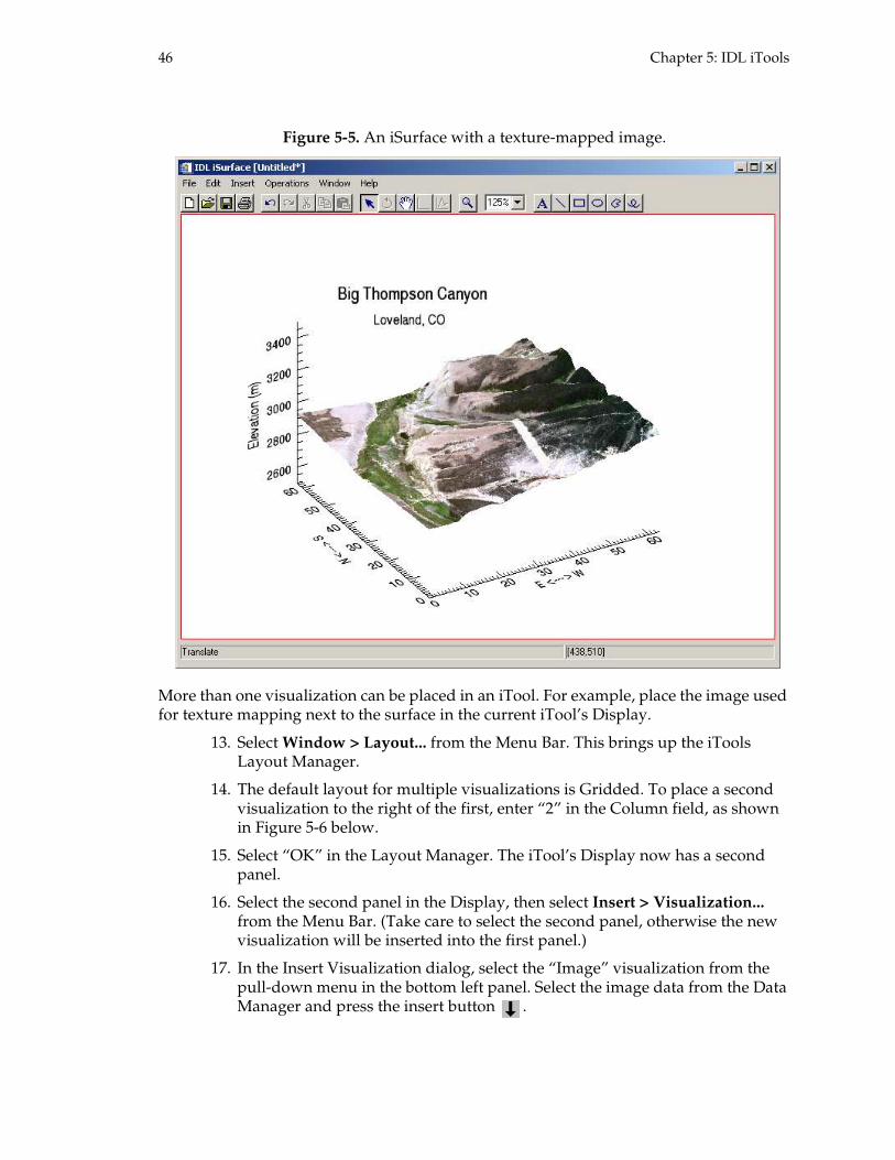
46 Chapter 5: IDL iTools
Figure 5-5. An iSurface with a texture-mapped image.
More than one visualization can be placed in an iTool. For example, place the image used for texture mapping next to the surface in the current iTool’s Display.
13. Select Window > Layout... from the Menu Bar. This brings up the iTools Layout Manager.
14. The default layout for multiple visualizations is Gridded. To place a second visualization to the right of the first, enter “2” in the Column field, as shown in Figure 5-6 below.
15. Select “OK” in the Layout Manager. The iTool’s Display now has a second panel.
16. Select the second panel in the Display, then select Insert > Visualization... from the Menu Bar. (Take care to select the second panel, otherwise the new visualization will be inserted into the first panel.)
17. In the Insert Visualization dialog, select the “Image” visualization from the pull-down menu in the bottom left panel. Select the image data from the Data Manager and press the insert button .

Chapter 5: IDL iTools 47
Figure 5-6. The iTools Layout Manager.
18. Select “OK” in the Insert Visualization dialog. The image will be displayed in the panel to the right of the surface visualization in the iTool’s Display.
Output the visualization in this iTool to a standard image file format.
19. From the Menu Bar, select File > Export... This brings up the File Export Wizard, which guides a user through three steps for output from a iTool.
Step 1: Select “To a File.” Click the “Next>>” button to proceed.
Step 2: Select one of the Views to export, or select the Window to export both. Click “Next>>.”
Step 3: Select a standard image file type, such as PNG or JPEG, then select a file name. Click “Finish” and the contents of the window will be written to the image file. View the image in a web browser.
Note that with the same series of steps, output can be directed to an Encapsulated PostScript file, using either an RGB or a CMYK color model. This form of output is especially useful for inclusion in a Microsoft Office or LaTeX document. Many scholarly journals require submission of graphics in Encapsulated PostScript.
The iTools Display can also be copied (using Edit > Copy from the Menu Bar or Ctrl+C on the keyboard) to the OS clipboard, then pasted into (for example) a Microsoft Office or an OpenOffice.org document.
The visualization in the Display can also be sent directly to a printer.
20. Start by selecting File > Print Preview... from the Menu Bar. Though this step is not necessary, it allows you to see what the printed page should look like. In the Print Preview window, you can use the black blocks in the margins to scale and position the visualization on the page, or use the “Center” button to center it automatically. You can also control the printer properties and print directly from this window.

48 Chapter 5: IDL iTools
21. To print without previewing, select File > Print from the menu bar, or click the Print button on the Tool bar or use the keyboard shortcut Ctrl+P .
The current state of an iTool can be saved as an iTools State (.isv) file. The state file can be opened on any other computer running the current version of IDL.
22. To save the current iTool state, select File > Save from the Menu Bar, the Save button on the Tool Bar, or use the keyboard shortcut Ctrl+S . Any of these selections spawns the OS-native file browser, where you can enter a name and location for a .isv file.
23. Close the current iTool with File > Exit.
24. Open a new iTool. Note that the particular iTool doesn’t matter.
IDL> isurface
25. Restore the .isv file by selecting File > Open... from the Menu Bar, the Open button on the Tool Bar, or by using the keyboard shortcut Ctrl+O . Any of these selections spawns the OS-native file browser, where you can find and select the .isv file. The former state of the iTool, including all visualizations and annotations, is restored in the current iTool.
Getting help
The Help selection on the Menu Bar can be used to get information on the iTools system. Further information on the general aspects of using the iTools can be found in Chapters 2 and 3 of the iTool User’s Guide, accessible from the IDL Online Help system.
Additionally, RSI has developed a series of recorded web seminars on the features and use of IDL, including two iTools tutorials. For more information, including instructions on how to download and view the web seminars, visit RSI’s web seminar page at http://www.rsinc.com/webinar .
Exercises
1. Experiment with the using the Line Profile button on the Tool Bar to trace the elevation change along a route in the Big Thompson Canyon DEM.
2. Try deleting and reinserting an axis in an iTools visualization. (Hint: there are at least two ways to do each.)
Suggested reading
Research Systems. Getting Started with IDL. Boulder, Colorado: Research Systems, 2005.
This document gives many tutorial-like examples of using IDL that are suitable for new users. From the Contents tab of the IDL Online Help utility, select User’s Guides > Getting Started with IDL.

Chapter 5: IDL iTools 49
Research Systems. iTool User’s Guide. Boulder, Colorado: Research Systems, 2005.
An explanation of how to use the new IDL iTools, along with many examples. This document can be accessed in the same manner as Getting Started with IDL, described above.

50 Chapter 5: IDL iTools

51
Chapter 6:
Line Plots
This chapter describes how to create two- and three-dimensional plots of point and line data, using the Direct Graphics PLOT procedure and the IPLOT iTool.
Introduction . . . . . . . . . . . . . . . . . . . . . . . . . . . 52Plotting: Direct Graphics . . . . . . . . . . . . . . . . . 52 Axis titles . . . . . . . . . . . . . . . . . . . . . . . . . . . . . 53 Axis ranges . . . . . . . . . . . . . . . . . . . . . . . . . . . 54 Axis styles . . . . . . . . . . . . . . . . . . . . . . . . . . . . 54 Line styles and symbols . . . . . . . . . . . . . . . . 55 Multiple data sets . . . . . . . . . . . . . . . . . . . . . . 56 Color . . . . . . . . . . . . . . . . . . . . . . . . . . . . . . . . . 57 Averaging or removing points . . . . . . . . . . . 58
Logarithmic axes . . . . . . . . . . . . . . . . . . . . . . 59 Multiple axes . . . . . . . . . . . . . . . . . . . . . . . . . 59Plotting: iTools . . . . . . . . . . . . . . . . . . . . . . . . 61 Visualization properties . . . . . . . . . . . . . . . . 62 Axis properties . . . . . . . . . . . . . . . . . . . . . . . 62 Plot properties . . . . . . . . . . . . . . . . . . . . . . . . 64Exercises . . . . . . . . . . . . . . . . . . . . . . . . . . . . . . 65Suggested reading . . . . . . . . . . . . . . . . . . . . . 66

52 Chapter 6: Line Plots
Introduction
Beginning with IDL 6.0, there are two interfaces for displaying point and line data: the first is the traditional Direct Graphics interface, with routines such as PLOT, OPLOT and PLOTS; the second is the new iTools interface with the IPLOT procedure.
This chapter is split into two parts. In the first, we plot data using the Direct Graphics routines. In the second, we plot data using the iTools.
A single data set, consisting of 24 hours of 5-min average values of meteorological variables from the NCAR Mesa Lab (ML) weather station, is used in this chapter. You can view the current data from this weather station at http://www.atd.ucar.edu/cgi-bin/weather.cgi?site=ml .
Use LOAD_DATA to read in temperature and dewpoint data sets, as well as a time stamp, from the ML weather station.
IDL> temp = load_data(’mesa_temp’)IDL> dewp = load_data(’mesa_dewp’)IDL> time = load_data(’mesa_time’)IDL> help, temp, dewp, timeTEMP FLOAT = Array[288]DEWP FLOAT = Array[288]TIME FLOAT = Array[288]
Each array consists of a sequence of 288 floating point values. In the following sections, we display these data in a variety of ways.
Plotting: Direct Graphics
View the sequence of temperature values with the PLOT procedure.
IDL> plot, temp
PLOT can only operate on array data. When PLOT is called with one parameter, that parameter is plotted versus its index values. PLOT can also be called with two parameters—the first representing the independent data, the second the dependent data. Plot temperature versus time.
IDL> plot, time, temp
The time axis is in units of seconds after 0000 UTC (1800 MDT). For plotting purposes, it may be more convenient to scale time into hours instead of seconds.
IDL> time = time/60.0^2IDL> plot, time, temp
Compare your results to Figure 6-1. This figure gives an example of the default look of the PLOT procedure. The default characteristics in a graphic generated with PLOT can be altered through the use of keyword arguments, a theme we explore in the next several sections. See the Online Help for more information on the PLOT procedure, including a complete list of its keywords.

Chapter 6: Line Plots 53
Figure 6-1. A plot of temperature (dependent axis) versus time (independent axis).
Axis titles
One problem with Figure 6-1 is that without context, there is no way of determining what is being plotted. Displaying labels on the coordinate axes would help to better describe this graphic.
Add descriptive titles to the plot axes using the XTITLE and YTITLE keywords to the PLOT procedure.
IDL> plot, time, temp, xtitle=’Time (UTC)’, ytitle=’Temp erature (C)’
Note that whenever PLOT is called, it erases the current contents of the window.
Add a title to the plot using the TITLE keyword. (Don’t forget to use the up arrow on your keyboard to retrieve the previous statement for editing—it’s a lot faster that retyping the entire statement).
IDL> plot, time, temp, xtitle=’Time (UTC)’, $IDL> ytitle=’Temperature (C)’, $IDL> title=’NCAR Mesa Lab Temperature: 2002-06-26’
You can control the character size of the titles with the [XYZ]CHARSIZE keywords. The overall size of the text produced by PLOT is controlled with CHARSIZE keyword. These keywords accept values relative to the default character size.
IDL> plot, time, temp, xtitle=’Time (UTC)’, xcharsize=0. 75, $IDL> ytitle=’Temperature (C)’, ycharsize=1.5
54 Chapter 6: Line Plots
Axis ranges
Determine the range of the temperature values using the MIN and MAX functions.
IDL> print, min(temp), max(temp)16.2000 30.3000
By default, IDL attempts to round axis ranges when plotting. For the case of the ML data, this results in the range 0-40oC shown in Figure 6-1. The range of an axis can be set with the [XYZ]RANGE keywords. Set the y-axis to range between 15 and 35oC using the YRANGE keyword.
IDL> plot, time, temp, yrange=[15,35]
The ordering of data in a plot can be reversed by swapping the minimum and maximum values used with the [XYZ]RANGE keywords. For example, to reverse the direction of the temperature axis, type
IDL> plot, time, temp, yrange=[35,15]
Now look at the range of the horizontal (time) axis in Figure 6-1. The data values for time range between 0 and almost 24 (hours in a day). IDL sets the axis range from 0 to 25 in the figure. Try setting the x-axis to range between 0 and 24 using the XRANGE keyword.
IDL> plot, time, temp, xrange=[0,24]
The range doesn’t change—it remains 0-25! To force IDL to use a specific axis range, use the [XYZ]STYLE keywords, discussed next.
Axis styles
The PLOT procedure defaults to using box axes with automatically calculated ranges. The [XYZ]STYLE keywords to PLOT can be used to alter these defaults. For example, to disable automatic scaling of the x-axis range, set the XSTYLE keyword to 1:
IDL> plot, time, temp, xstyle=1
The time axis now spans the range 0-24.
To remove all axes from the plot, set both XSTYLE and YSTYLE keywords to 4:
IDL> plot, time, temp, xstyle=4, ystyle=4
To remove only the top x-axis, set the XSTYLE keyword to 8:
IDL> plot, time, temp, xstyle=8
To disable autoscaling on both axes and remove the right and top axes, type:
IDL> plot, time, temp, xstyle=9, ystyle=9
Compare your results with Figure 6-2 below.

Chapter 6: Line Plots 55
Figure 6-2. A plot of temperature versus time with autoscaling and box axes disabled.
Line styles and symbols
The line style used by PLOT can be controlled with the LINESTYLE keyword. Plot symbols are controlled with the PSYM keyword. A complete list of line styles and plot symbols is given in Table 6-1.
By default, PLOT uses a solid line and no plot symbol. To display the ML temperature data with a dashed line, set the LINESTYLE keyword to 2:
IDL> plot, time, temp, linestyle=2
Table 6-1. Line styles and plot symbols for the PLOT procedure.
Index Line style Plot symbol
0 solid no symbol
1 dotted plus
2 dashed asterisk
3 dash dot period
4 dash dot dot diamond
5 long dash triangle
6 square
7 x
8 user-defined
9
10 histogram

56 Chapter 6: Line Plots
The thickness of the line is controlled with the THICK keyword. The default line thickness is 1. Display the data with a double-weight dashed line:
IDL> plot, time, temp, linestyle=2, thick=2
To display the temperature data with triangles, set the PSYM keyword to 5:
IDL> plot, time, temp, psym=5
The size of the plot symbols is indicated by the SYMSIZE keyword. The default symbol size is 1. Make symbols that are half the normal size:
IDL> plot, time, temp, psym=5, symsize=0.5
To display the data with both a line style and a symbol, the value of the PSYM keyword needs to be negative; otherwise only the symbol is plotted, the line is ignored. Display the ML temperature data with a dashed line and triangles, limiting the range on the time axis so that it’s easier to see the line connecting the symbols:
IDL> plot, time, temp, linestyle=2, psym=-5, xrange=[5,1 5], /ynozero
The YNOZERO keyword instructs PLOT to ignore the value of zero in creating an autoscaled y-axis.
The USERSYM procedure
The USERSYM procedure allows a user to construct a plot symbol for PSYM index 8. Symbols are drawn with vectors. The symbols can be of any size, can have up to 50 vertices and can be filled. The following code creates a plot symbol in the form of an upside-down, filled triangle.
IDL> load_colorsIDL> x_points = [0, 1, -1, 0]IDL> y_points = [-1, 1, 1, -1]IDL> usersym, x_points, y_points, /fill, color=100
Use this plot symbol to display a portion of the ML temperature data.
IDL> plot, time, temp, psym=8, xrange=[5,15], /ynozero
Compare your results with Figure 6-3 below.
Multiple data sets
The OPLOT procedure is used to display vector data over a previously drawn plot. OPLOT can only be called after PLOT. OPLOT uses the axes and coordinate system that are set up by PLOT.
For example, plot the ML temperature data using PLOT, then overplot the dewpoint data with a different linestyle using OPLOT:
IDL> plot, time, tempIDL> oplot, time, dewp, linestyle=2

Chapter 6: Line Plots 57
Figure 6-3. A plot with user-defined symbols created with USERSYM.
Color
Two keywords, COLOR and BACKGROUND, control the use of color in line plots. COLOR controls the foreground color, including the color of the data symbols or line styles, the axes and any titles. BACKGROUND controls the background color. Note that these keywords only accept scalar values, regardless of whether IDL is in indexed or in decomposed color mode. For more information about IDL color modes, see Chapter 4, “Graphics Systems” in this manual.
Indexed color mode
In indexed color mode, the values for the COLOR and BACKGROUND keywords represent entries into the current color table.
Set indexed color mode and load a predefined color table into IDL.
IDL> device, decomposed=0IDL> loadct, 5
Plot the ML temperature data with a yellow color on a blue background:
IDL> plot, time, temp, color=200, background=50
What relationship do yellow and blue have with the numbers 200 and 50? Use XPALETTE to view the entries in color table 5.
IDL> xpalette

58 Chapter 6: Line Plots
The index value 200 in color table 5 corresponds to the RGB triple (255,255,77), a yellowish color. Likewise, the index 50 corresponds, in this color table, to the RGB triple (14,0,250), a blue color.
Dismiss XPALETTE by clicking either its "Done" button or the operating system close button.
Decomposed color mode
In decomposed color mode, the values for the COLOR and BACKGROUND keywords are used to directly specify a color from the RGB color system.
Set decomposed color mode.
IDL> device, decomposed=1
It would be convenient to directly specify an RGB triple as the value for the COLOR and BACKGROUND keywords. To reproduce the yellow-foreground, blue-background plot above we could just type
IDL> plot, time, temp, color=[255,255,77], background=[1 4,0,250]% PLOT: Expression must be a scalar or 1 element ar ray % in this context: <INT Array[3]>.% Execution halted at: $MAIN$
Unfortunately, this doesn’t work. IDL expects a single scalar value as input to these keywords, not an array of values. What does work is specifying the color as a hexadecimal value, as in HTML:
IDL> plot, time, temp, color=’4DFFFF’xL, background=’FA0 00E’xL
Easier still, the course program RGB2IDX can be used.
IDL> fore = rgb2idx([255,255,77])IDL> back = rgb2idx([14,0,250])IDL> plot, time, temp, color=fore, background=back
Switch back to indexed color mode.
IDL> device, decomposed=0
We use indexed color mode for most of the examples in this manual.
Averaging or removing points
Data can be block-averaged prior to display using the NSUM keyword to PLOT. Set NSUM to the width of the averaging filter. For example, block-average every three dewpoint values in the ML data set and display:
IDL> plot, time, dewp, nsum=3
This is the equivalent of using the REBIN function on the data.
IDL> n_points = n_elements(time)IDL> plot, rebin(time, n_points/3), rebin(dewp, n_points /3)

Chapter 6: Line Plots 59
Outliers can be excluded from a line plot by setting the MAX_VALUE and MIN_VALUE keywords. For example, plot the ML temperature values, but exclude any values that are less than 20oC.
IDL> plot, time, temp, min_value=20
Individual data points can also be excluded. This can be useful for removing missing or defective data points from a plot. Assign the IEEE not a number (NaN) value, stored in the IDL system variable !values.f_nan (more on system variables in Chapter 7, “Variables”) to individual points to remove them from a plot.
Logarithmic axes
By default, PLOT uses linear axis scales. By setting the [XYZ]LOG keywords, axes can be forced to use a logarithmic scale. For example, plot a straight line on a logarithmic x-axis:
IDL> plot, findgen(100), /xlog, xrange=[0.1, 100]
Don’t forget that the value zero cannot be represented on a logarithmic axis.
Now plot the line with a logarithmic y-axis:
IDL> plot, findgen(100), /ylog, yrange=[1e-1, 1e2]
Note that IDL understands numbers typed in scientific notation.
Now plot the line with logarithmic x- and y-axes:
IDL> plot, findgen(100), /xlog, xrange=[1e-1, 1e2], /ylo g
Multiple axes
It is often convenient to compare more than one set of data in a single graphic. When data sets share a common range, they can be displayed on common axes; otherwise, separate axes are needed. The AXIS procedure is used to add to—or replace—the axes displayed by the PLOT procedure.
Here’s an example. Use LOAD_DATA to read in the wind speed and wind direction data from the ML weather station.
IDL> wspd = load_data(’mesa_wspd’)IDL> wdir = load_data(’mesa_wdir’)IDL> help, wspd, wdirWSPD FLOAT = Array[288]WDIR FLOAT = Array[288]
What are the ranges of these data?
IDL> print, max(wspd), max(wdir)11.0000 356.000
Wind speed ranges between 0 and 11 ms-1, while wind direction varies between 0 and 360o from north. It would be difficult to construct a legible graphic if these data were displayed on the same axes. We’ll attempt to make a graphic that has separate color-coded axes for each data set.

60 Chapter 6: Line Plots
Start by setting up a plot that has no y-axes (by setting YSTYLE to 4) and no data displayed (by setting the NODATA keyword). A color-coded axis will be constructed for each data set. The XMARGIN keyword is used to produce an equal amount of space to the right and left of the plot, leaving room for axis titles.
IDL> plot, time, wspd, ystyle=4, xstyle=1, /nodata, $IDL> xtitle=’Time (UTC)’, xmargin=[10,10]
Create a new y-axis for the wind speed with the AXIS procedure. Setting the YAXIS keyword to 0 produces a y-axis on the left side of the plot. Display the wind speed data with OPLOT. The axis and the data use the same blue color (index 50 in table 5).
IDL> axis, yaxis=0, ytitle=’Wind Speed (m/s)’, color=50IDL> oplot, time, wspd, color=50, linestyle=2
Display an axis for wind direction on the right side of the plot with AXIS by setting the YAXIS keyword to 1. The range for the wind direction data is set with YRANGE. The SAVE keyword is crucial for this axis. SAVE redefines the plot axis range to use the setting for the YRANGE keyword; without it, the wind direction data would be plotted on the same range as the wind speed data. The YTICKS keyword specifies the number of major intervals on the axis. The YMINOR keyword specifies the number of minor intervals between the major ticks.
IDL> axis, yaxis=1, yrange=[0,360], ystyle=1, yticks=4, yminor=3, $IDL> ytitle=’Wind Direction (deg)’, color=110, /save
Finally, display the wind direction data with OPLOT.
IDL> oplot, time, wdir, color=110
Compare your results with Figure 6-4 below.
Figure 6-4. A plot of wind speed (dashed) and direction (solid) with two dependent axes.

Chapter 6: Line Plots 61
Plotting: iTools
The purpose of the IPLOT iTool is to display vector data with Object Graphics, much like the PLOT procedure does with Direct Graphics. IPLOT, however, has greater flexibility in manipulating and visualizing data.
Display the ML temperature time series with IPLOT.
IDL> iplot, time, temp
The default look of IPLOT in displaying this time series is shown in Figure 6-5.
Figure 6-5. The ML temperature time series displayed in an iTool.
The default characteristics in a graphic generated with IPLOT can be altered either through the use of keyword arguments or by directly manipulating the properties of the graphic with the mouse. We’ll explore both techniques in the following sections. The Online Help also has more information on the IPLOT procedure, including a complete list of its keywords.

62 Chapter 6: Line Plots
Visualization properties
All aspects of the graphics displayed in Figure 6-5 can be altered through the iTools Visualization Browser. The Visualization Browser is introduced in “An overview of the iTools” on page 40, and is discussed in more detail there. Open the Visualization Browser by selecting Window > Visualization Browser... in the current iTool.
Axis properties
Properties of individual axes or all axes can be changed in an iTools visualization. Start by adding axis titles to the current iTool.
1. In the iTool, double-click on the x-axis with the left mouse button. This opens the Visualization Browser and causes it to display a list of all the properties associated with this axis.
2. Scroll through the list of properties in the right panel of the Visualization Browser to find the Title property. Click on this property and enter Time (UTC) in its text field. Hit the "Enter" key. The axis title now appears in the iTool.
3. Return to the iTool and click on the y-axis. The Visualization Browser updates to show properties of the y-axis.
4. Enter Temperature (C) in the Title property for the y-axis. Hit the "Enter" key.
The iTool now displays the ML temperature time series with appropriate axis titles. These changes could also be made programmatically through the use of the [XYZ]TITLE keywords:
IDL> iplot, time, temp, xtitle=’Time (UTC)’, ytitle=’Tem perature (C)’
Axis properties such as fonts and color can be controlled through the iTools Visualization Browser.
1. In the left panel of the Visualization Browser, select the Axes graphic element. The properties displayed in the right panel of the Visualization Browser now refer to all axes in the visualization. Selecting Axis 0 refers to the lower x-axis, Axis 1 refers to the upper x-axis, etc.
2. Scroll through the property list in the Visualization Browser to find Text color. Select this entry to change the color of one or all of the axes. You can choose colors from a predefined palette, or you can build your own custom color from the RGB color system. The display is updated automatically.
3. Try changing the Text font, Text style and Text font size properties, as well.
These axis properties can be altered programmatically using the [XYZ]TEXT_COLOR, [XYZ]TICKFONT_INDEX, [XYZ]TICKFONT_STYLE and [XYZ]TICKFONT_SIZE keywords.
Axis styles can be modified quickly with the Visualization Browser. For example, to remove the top and right axes in the current iTool:

Chapter 6: Line Plots 63
1. In the left panel of the Visualization Browser, select the Axis 1 graphic element.
2. Find the Show property for this axis and change it to False.
3. Perform the same operation on Axis 3. In each case, the display updates automatically.
Axis ranges can be set programmatically through the [XYZ]RANGE keywords, or modified interactively in the Visualization Browser through the Data Space graphic element.
Figure 6-6 demonstrates a few of the modifications discussed above to the default x and y axes in an iTool.
Figure 6-6. The ML temperature time series with axis formatting changes.

64 Chapter 6: Line Plots
Plot properties
Properties of the plot line can be changed in an iTools visualization. Here, we work with the plot color.
1. In the iTool, double-click on the plot line with the left mouse button. This opens the Visualization Browser, which displays a list of all the properties associated with the plot.
2. The current color is displayed in the Color entry in the Visualization Browser. Select this entry to change the color. You can choose from a predefined palette, or you can build your own custom color from the RGB color system. The display is updated automatically.
These changes could also be accomplished programmatically through the use of the COLOR keyword. For example, to plot the ML temperature time series in red, type:
IDL> iplot, time, temp, xtitle=’Time (UTC)’, $IDL> ytitle=’Temperature (C)’, color=[255,0,0]
The COLOR keyword to IPLOT accepts an RGB triple, unlike the COLOR keyword to PLOT, as discussed in the section “Color” on page 57.
The background color of the plot area—and of the iTool itself—can also be changed.
1. Open the iTools Visualization Browser.
2. Select the Data Space graphic element from the left panel of the Browser.
3. Scroll to the bottom of the Visualization Browser’s right panel. With the Fill background entry set to True, choose a color from the Fill color entry and select a Transparency value of 50. The background of the plot will now be filled with the selected color at a 50 percent intensity.
4. To change the background color of the iTool itself, select the Visualization Layer graphic element from the left panel of the Visualization Browser.
5. Change the Background color property to a setting of your choice.
Programmatically, these changes could be made with the FILL_BACKGROUND, FILL_COLOR, FILL_LEVEL and TRANSPARENCY keywords to IPLOT.
Add a finishing touch to this visualization by creating a legend.
1. Click on the plot with the left mouse button.
2. Select Insert > Legend from the iTools menu bar. A legend containing the name of the data set appears in the iTool.
3. Double-click on the legend, bringing up the Visualization Browser. Edit the text of the legend by changing the Text property in the right panel of the Browser.
4. Position the legend in the iTool by dragging it with the mouse.
Compare your results with Figure 6-7.
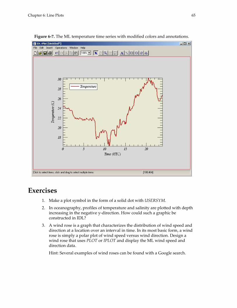
Chapter 6: Line Plots 65
Figure 6-7. The ML temperature time series with modified colors and annotations.
Exercises
1. Make a plot symbol in the form of a solid dot with USERSYM.
2. In oceanography, profiles of temperature and salinity are plotted with depth increasing in the negative y-direction. How could such a graphic be constructed in IDL?
3. A wind rose is a graph that characterizes the distribution of wind speed and direction at a location over an interval in time. In its most basic form, a wind rose is simply a polar plot of wind speed versus wind direction. Design a wind rose that uses PLOT or IPLOT and display the ML wind speed and direction data.
Hint: Several examples of wind roses can be found with a Google search.

66 Chapter 6: Line Plots
Suggested reading
Research Systems. Getting Started with IDL. Boulder, Colorado: Research Systems, 2005.
Chapter 3, “2-D Plots” describes and gives examples of the use of the Direct Graphics and iTools line plotting routines. From the Contents tab of the IDL Online Help utility, select User’s Guides > Getting Started with IDL.
Research Systems. iTool User’s Guide. Boulder, Colorado: Research Systems, 2005.
Chapter 13 of this manual discusses the use of the iPlot iTool. From the Contents tab of the IDL Online Help utility, select User’s Guides > iTool User’s Guide.

67
Chapter 7:
Variables
Variables have an associated data type and organization (scalar, array, or structure).
IDL has a rich set of data types for integer, floating point, string and abstract data. Conversion between the types is straightforward.
IDL is an array-based language. Operators and many library routines work on both arrays and scalars.
Introduction to variables . . . . . . . . . . . . . . . . . 68 Valid names . . . . . . . . . . . . . . . . . . . . . . . . . . . 68 Variable types . . . . . . . . . . . . . . . . . . . . . . . . . 68 Variable creation . . . . . . . . . . . . . . . . . . . . . . . 69Scalars . . . . . . . . . . . . . . . . . . . . . . . . . . . . . . . . 70Arrays . . . . . . . . . . . . . . . . . . . . . . . . . . . . . . . . 70 Creation . . . . . . . . . . . . . . . . . . . . . . . . . . . . . . 70 Subscripting . . . . . . . . . . . . . . . . . . . . . . . . . . 71 Operating on arrays . . . . . . . . . . . . . . . . . . . . 72 Multi-dimensional arrays . . . . . . . . . . . . . . . 72 Single index subscripting . . . . . . . . . . . . . . . 73Structures . . . . . . . . . . . . . . . . . . . . . . . . . . . . . . 74 Named structures . . . . . . . . . . . . . . . . . . . . . . 74 Anonymous structures . . . . . . . . . . . . . . . . . 75
Working with structures . . . . . . . . . . . . . . . 76Working with variables . . . . . . . . . . . . . . . . . 77 The byte exception . . . . . . . . . . . . . . . . . . . . 77 Variables are dynamic . . . . . . . . . . . . . . . . . 78 Expression type and structure . . . . . . . . . . 79 Using the wrong variable type . . . . . . . . . . 79 Be aware of short integers . . . . . . . . . . . . . . 80System variables . . . . . . . . . . . . . . . . . . . . . . . 80 Informational . . . . . . . . . . . . . . . . . . . . . . . . . 80 IDL environment . . . . . . . . . . . . . . . . . . . . . . 80 Direct Graphics output . . . . . . . . . . . . . . . . 81Exercises . . . . . . . . . . . . . . . . . . . . . . . . . . . . . . 82Suggested reading . . . . . . . . . . . . . . . . . . . . . 83

68 Chapter 7: Variables
Introduction to variables
The primary purpose of the Data statement is to give names to constants; instead of referring to pi as 3.141592653589793 at every appearance, the variable Pi can be given that value with a Data statement and used instead of the longer form of the constant. This also simplifies modifying the program, should the value of pi change.
— Fortran manual for Xerox Computers
Valid names
Variable names must start with a letter or an underscore and may contain up to 128 letters, digits, underscores, or dollar signs. The size of a variable (i.e., the amount of memory allocated to a variable) is limited only by the computer and operating system you are using, not by IDL. Variable names are case-insensitive; IDL converts all alphabetic characters to uppercase internally.
Here are examples of valid variable names:
read6_$fileonly_8_bitComputerTypevariable2_day_of_yearprintIDL
Here are examples of invalid variable names:
name.lastthird%file4th_list$tempcase
The IDL_VALIDNAME function determines whether a string may be used as a valid IDL variable name. It can optionally convert non-valid characters into underscores, returning a valid name string. For example,
IDL> print, idl_validname(’variable2’)variable2IDL> print, idl_validname(’4th_list’)
IDL> print, idl_validname(’4th_list’, /convert_all)_4th_listIDL> print, idl_validname(’i d l’, /convert_spaces)i_d_l
Variable types
There are 16 variable types in IDL, seven integer, two floating point, two complex, a string type, two abstract types (pointers and objects), and undefined. Structures are considered their own type, while arrays are considered the same type as their elements. See the overview of IDL types in Table 7-1.

Chapter 7: Variables 69
Variable creation
Variables do not have to be declared in IDL. The type of a variable is determined by its usage. If a variable is set equal to the sum of two floating point values, the result is a float. IDL variables can easily be converted between types using the functions listed in the “Conversion Function” column of Table 7-1. Before creation, a variable is of the undefined type; it is illegal to use an undefined variable in an expression.
IDL> help, varVAR UNDEFINED = <Undefined>IDL> var = 0LIDL> help, varVAR LONG = 0
There are three valid organizations for IDL variables:
• scalars,
• arrays (from one to eight dimensions of a single type), and
• structures (an aggregate of other data types and organizations).
We will consider each of the type organizations in turn.
Table 7-1. IDL variable types.
TypeSize
(bytes)Type code
Range Scalar creation notationConversion function
byte 1 1 0–255 a = 5B BYTE
integer 2 2 ±2^15-1 b = 0S ; b = 0 FIX
unsigned integer 2 12 0–2^16-1 c = 0U UINT
long integer 4 3 ±2^31-1 d = 0L LONG
unsigned long integer
4 13 0–2^32-1 e = 0UL ULONG
64-bit integer 8 14 ±2^63-1 f = 0LL LONG64
unsigned 64-bit integer
8 15 0–2^64-1 g = 0ULL ULONG64
float 4 4 h = 0.0 FLOAT
double 8 5 i = 0.0D DOUBLE
complex 8 6 j = complex(1.0,0.0) COMPLEX
double complex 16 9 k = dcomplex(1.0,0.0) DCOMPLEX
string 7 l = 'hello'
l = "hello"
STRING/
STRTRIM
pointer 4 10 m = ptr_new()
object 4 11 n = obj_new()
undefined 1 0
structure 8 see “Structures” on page 74 for more detailed information

70 Chapter 7: Variables
Scalars
Scalar variables are initialized by setting the variable equal to a scalar value, a scalar variable, or an expression that evaluates to a scalar. Use the notation in the “Creation” column of Table 7-1 to create a variable of a specify type. For example:
IDL> image_pixel = 0B ; byte IDL> loopcounter = 0U ; uintIDL> n_elms = 0L ; longIDL> fileoffset = 0ULL ; ulong64IDL> variance = 0.0 ; floatIDL> total = 0.0D ; doubleIDL> complex_var = complex(0.0, 0.0) ; complexIDL> name = ’Hello World’ ; stringIDL> new_image_pixel = image_pixel ; byteIDL> pixel_value = image_pixel + 0.0 ; byte + float = fl oat
The variable names on the left side of the equal sign take on the type of the value, variable, or expression on the right side.
Arrays
IDL is an array based language; there is useful syntax for indexing subarrays and operating on arrays. Appropriate use of the syntax makes code both faster and easier to read.
Creation
Vectors and arrays of the different variable data types can be set or initialized with the IDL routines listed in Table 7-2
IDL> vec = fltarr(15)IDL> vec[5] = 4.56IDL> vec[13] = 1234.333
IDL array subscripts always begin with 0; therefore the vec array has valid subscripts from 0 to 14.
Arrays can also be created by setting a variable equal to a list of values enclosed in square brackets.
IDL> temp = [12, 82, 97, 23, 0, 78]
This statement creates an array of six integers. Multiple-dimension arrays can also be created with square brackets with multiple sets of brackets, as in:
IDL> id4x4 = [[1,0,0,0], [0,1,0,0], [0,0,1,0], [0,0,0,1] ]IDL> help, id4x4ID4X4 INT = Array[4, 4]
The id4x4 variable becomes a integer matrix. Consider the statement below:
IDL> example_arr = [3.4, 6.7D, 45U, 90L]
4 4×
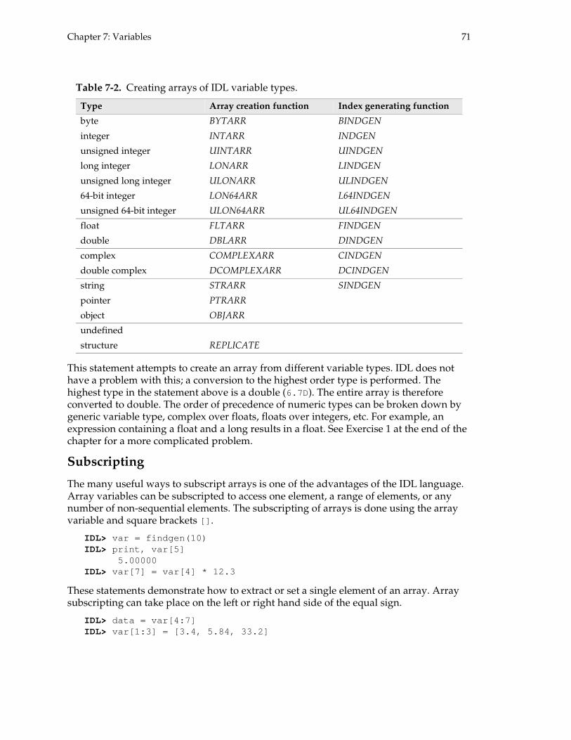
Chapter 7: Variables 71
This statement attempts to create an array from different variable types. IDL does not have a problem with this; a conversion to the highest order type is performed. The highest type in the statement above is a double (6.7D ). The entire array is therefore converted to double. The order of precedence of numeric types can be broken down by generic variable type, complex over floats, floats over integers, etc. For example, an expression containing a float and a long results in a float. See Exercise 1 at the end of the chapter for a more complicated problem.
Subscripting
The many useful ways to subscript arrays is one of the advantages of the IDL language. Array variables can be subscripted to access one element, a range of elements, or any number of non-sequential elements. The subscripting of arrays is done using the array variable and square brackets [] .
IDL> var = findgen(10)IDL> print, var[5]
5.00000IDL> var[7] = var[4] * 12.3
These statements demonstrate how to extract or set a single element of an array. Array subscripting can take place on the left or right hand side of the equal sign.
IDL> data = var[4:7]IDL> var[1:3] = [3.4, 5.84, 33.2]
Table 7-2. Creating arrays of IDL variable types.
Type Array creation function Index generating function
byte BYTARR BINDGEN
integer INTARR INDGEN
unsigned integer UINTARR UINDGEN
long integer LONARR LINDGEN
unsigned long integer ULONARR ULINDGEN
64-bit integer LON64ARR L64INDGEN
unsigned 64-bit integer ULON64ARR UL64INDGEN
float FLTARR FINDGEN
double DBLARR DINDGEN
complex COMPLEXARR CINDGEN
double complex DCOMPLEXARR DCINDGEN
string STRARR SINDGEN
pointer PTRARR
object OBJARR
undefined
structure REPLICATE
72 Chapter 7: Variables
The first statement creates a new array, data, that contains elements 4 through 7 of var. The resulting array is a floating point array of 4 elements. The next statement sets elements 1 through 3 of var to the array specified on the right hand side of the equation.
IDL> var[5:9] = 3.5
This statement sets elements 5 through 9 equal to the value 3.5. An array range must be assigned to a single value or an array of equal length. An error occurs if the array range is set to an array less than or greater than the number of elements in the range.
IDL> var[5:9:2] = 2.2
“Strides” are used in the above example to set every 2nd element between indices 5 and 9 to the value 2.2.
IDL> var[3:*] = 4.999
An asterisk (* ) used in a subscript range indicates the end of the array. The statement above sets elements 3 to the end (9) of the array to the value 4.999. Used alone, the asterisk represents the entire array.
IDL> var[*] = 9.9
Subscript ranges do not have to be continuous. Non-sequential elements of an array can be accessed by subscripting an array with another array.
IDL> array = [-14, 41, -90, 67, 10]IDL> indices = [4, 2, 0, 1]IDL> print, array[indices]
10 -90 -14 41
The last statement prints elements 4, 2, 0 and 1 from array. This is a powerful method of subscripting that is used primarily with the IDL WHERE function.
Operating on arrays
When an operation is performed on an array in IDL, it is performed on every element in the array. This powerful feature eliminates the need to use loops to perform an operation on every element of an array.
IDL> x = findgen(360) * !dtorIDL> sincurve = sin(x)IDL> plot, sincurve
The first statement above multiplies the numbers 0.0, 1.0, 2.0, …359.0 by the degrees-to-radians constant, then the second statement takes the sine of every element of the result. This benefit of IDL eliminates the need to add time-consuming control loops to perform an operation on every element in an array. Take advantage of this behavior as much as possible—it is both faster and easier to read.
Multi-dimensional arrays
Arrays in IDL can have up to eight dimensions. In the two-dimensional case, IDL array subscripting is specified as [column, row].
IDL> multi = lindgen(4, 6) ; four columns, six rows
Chapter 7: Variables 73
IDL> print, multi0 1 2 3
4 5 6 7 8 9 10 11 12 13 14 15 16 17 18 19 20 21 22 23
The method of subscripting in IDL is column major. Internally, arrays are laid out in a row major format (the elements of multi are numbered in the order they are stored in memory). The subscripting of a two-dimensional array should be done using the [column, row] notation.
IDL> print, multi[1, 0], multi[3, 5]1 23
All of the range operators can also be used on multi-dimensional arrays.
IDL> print, multi[*, 4] ; the fifth row16 17 18 19
IDL> print, multi[2, *] ; the third column2610141822
IDL> print, multi[2:3, 1:2] ; a block in the middle - co l 3-4 row 2-36 710 11
Single index subscripting
Any IDL variable can be subscripted with a single index in array notation. This is even possible for scalars, though the only valid index is 0:
IDL> scalar = 5IDL> print, scalar[0]
5
The elements of a multi-dimensional array are indexed in the same order as they are numbered in the index generating function—the left-most index varies the fastest when traversing the array in order of the single index. In the two-dimensional case, see the example of lindgen(4, 6) above. For example,
IDL> print, multi[10]10
The ARRAY_INDICES function can be used to convert single index subscripts into dimensional subscripts.
IDL> print, array_indices(multi, 10)2 2
The result is the [column, row] index values corresponding to element 10 in multi.

74 Chapter 7: Variables
The WHERE function
The WHERE function evaluates an expression and returns the one-dimensional index of each element in an array for which the expression is true (it returns the locations, not the data values). If the expression is false, the return value is a one-element vector with the value -1. For example, to set all the elements in the array data that have values between 0.4 and 0.5 to the value 1.0, type:
IDL> x = findgen(360) * !dtorIDL> data = sin(x)IDL> indices = where(data gt 0.4 and data lt 0.5, count)IDL> data[indices] = 1.0
The WHERE function returns a vector containing subscript locations into the data array.
The statement above, data[indices] = 1 , is similar to the statement
IDL> data[ [2,4,6] ] = 1.0
since indices is a vector, as is [2,4,6] .
Multi-dimensional arrays can be passed to the WHERE function as well. For example,
IDL> d = dist(100)IDL> surface, dIDL> multi_ind = where(d gt 65, count)IDL> d[multi_ind] = 0.0IDL> surface, d
Syntactically, this is exactly the same as the single dimension case. The one subtlety is that the statement expression d[multi_ind] uses single index subscripting for the two dimensional array.
Structures
A structure in IDL is a collection of variables of different types. There are two types of IDL structure variables: named structures and anonymous structures.
Named structures
A named structure is a structure whose layout is stored under a unique name in IDL. When a named structure is created in IDL, its layout is remembered and can be used to create instances of that same layout. The components of a named structure are the name, the fields and the values. Curly braces are used exclusively for structure creation,
IDL> p1 = { point, x:1.0, y:3.0, color:bytarr(3) }
This statement defines a named structure, point, that contains three fields, x, y, and color. The structure is stored in the variable p1. The variable type of the fields of a structure are determined by the value used to define the field. In the case of the point structure above, the x and y fields are floats and color is a byte array. To find more information about a structure variable, use the STRUCTURE keyword to the HELP routine,
IDL> help, p1, /structure
Chapter 7: Variables 75
** Structure POINT, 3 tags, length=12, data length= 11: X FLOAT 1.00000 Y FLOAT 3.00000 COLOR BYTE Array[3]
Structure fields can also be initialized to variables. The current type of the variable determines the type of the field. Consider the example below.
IDL> a = 0ULIDL> b = 0.9IDL> c = 23.4DIDL> my1 = { mystruct, f1:a, f2:b, f3:c }
The named structure mystruct contains three scalar fields: an unsigned long, a float and a double.
Once a named structure is defined in IDL, fields cannot change size or type nor can they be added or removed from the structure. A named structure definition is set in IDL memory until the IDL session ends or is reset (using .reset_session ).
To create new instances of named structures, use curly brackets and the structure name.
IDL> p2 = { point }IDL> my2 = { mystruct }
The variable p2 contains a fresh copy of the point structure. When a new named structure is created in this manner, all the fields are zeroed or nulled (strings, pointers, objects) out; the values used to define the structure are not carried over.
IDL> help, p2, /structure** Structure POINT, 3 tags, length=12, data length= 11: X FLOAT 0.000000 Y FLOAT 0.000000 COLOR BYTE Array[3]
Accessing structure fields
To access a field of the structure, use the period operator with the field name,
IDL> print, p2.x0.000000
IDL> p2.y = 9.5IDL> p2.color = [255, 0, 255]IDL> my2.f1 = 44L
Structure fields can also be accessed by number.
IDL> print, p2.(0) ; same as p2.x0.000000
IDL> p2.(1) = 9.5 ; same as p2.yIDL> p2.(2) = [255, 0, 255] ; same as p2.colorIDL> my2.(0) = 44L ; same as my2.f1
Anonymous structures
Anonymous structures do not have a name associated with them.

76 Chapter 7: Variables
IDL> an1 = { lat:0.0, lon:0.0, ht:0L, pitch:0.0D }IDL> an1.lat = 12.4IDL> an1.pitch = 45.67
Since there is not a name associated with them, new anonymous structures can be defined with fields added or subtracted.
IDL> an1 = { lat:0.0, lon:0.0, ht:0L, pitch:0.0D, attitu de:0U }IDL> an2 = an1IDL> an2.pitch = 79.0D
Working with structures
Arrays of structures
To create an array of structures use the REPLICATE function. REPLICATE can be used to replicate data of any type but is most often used to create arrays of structures. The array created can either be a replicate structure name or a replicated structure variable.
IDL> ptarr = replicate({ point }, 5)IDL> ptarr[0].x = 5.6IDL> ptarr[0].y = 9.3
Each field of a structure array can be treated like individual arrays.
IDL> ptarr.x = 6.7
This statement sets the x field of all the structures in the array to 6.7
IDL> ptarr.y = findgen(5)
This statement sets the y field of all the structure to the result of the FINDGEN function.
Structure fields type and size
When a named or anonymous structure is created, the type and size of the fields are set and cannot be changed. When setting a value in a structure field, IDL will convert the value or variable to the type of the field. Any attempt to change the size of a structure field, such as re-dimensioning an array, causes an error.
IDL> anon = { name:’John’, age:34, height:69.5, grades:f ltarr(10) }IDL> anon.age = 45.5 ; value converted to inte gerIDL> anon.height = 70 ; value converted to floa tIDL> anon.grades[9] = 78.54D ; value converted floatIDL> anon.grades = fltarr(8) ; okay but field still co ntains 10 valuesIDL> anon.grades = intarr(10) ; okay but field still is fltarrIDL> help, anon, /structure** Structure <17218d0>, 4 tags, length=60, data len gth=60, refs=1: NAME STRING ’John’ AGE LONG 45 HEIGHT FLOAT 70.0000 GRADES FLOAT Array[10]IDL> anon.grades = fltarr(15) ; ERROR! attempt to resiz e field

Chapter 7: Variables 77
IDL is very flexible with conversions, but does not allow a field containing an array to be extended. This is possible using pointers, but is beyond the scope of this course.
Miscellaneous structure information
The field names of the structure can be returned in the form of a string array by using the TAG_NAMES function.
IDL> fnames = tag_names(p2)
TAG_NAMES can also be used to retrieve the name of a structure.
IDL> sname = tag_names(p2, /structure_name)
To find out number of fields in a structure use the N_TAGS function.
IDL> nf = n_tags(p2)
N_TAGS can also be used to find out the contiguous length in bytes of a structure.
IDL> slen = n_tags(p2, /length)
Named versus anonymous structures
Named structures are used in situations calling for a constant, clearly defined definition of a structure. Examples of using named structures are in the event structures in widget programs, class definitions in object-oriented programming, and other structures where the definition of the structure will not change at run-time.
Anonymous structures allow for a more fluid definition. Although anonymous structures cannot change definition at run-time, it is easier to simply to create another anonymous structure with an additional field (a named structure would have to have a new name). Examples of using anonymous structures are for reading ASCII data with different data types in columns, the “state” structure of a widget program, and ad hoc analysis. Unless there is a clear need to be able to create many structures with the exact same definition, anonymous structures are a good choice.
Working with variables
Like any language, there are a few areas which will catch the user unaware. With forewarning, these features of IDL prove to be useful as well.
The byte exception
The exception to the rule that alphabetic characters cannot convert to numbers is the byte type. When IDL converts a string of characters to bytes, the result is a byte array with the same length as the string. The elements of the byte array contain the ASCII value of each character in the string. Conversely, an array of bytes converted to a string results in a string containing the characters’ ASCII values.
IDL> str = ’Hello World’IDL> bstr = byte(str)IDL> help, bstrIDL> bstr[0] = bstr[0] + 5

78 Chapter 7: Variables
IDL> print, string(bstr)
These commands convert the string into an array of bytes and manipulate the first byte. Adding five to the first byte changes the ‘H’ to an ‘M’. Converting the bytes back to a string results in the string ‘Mello World.’
If a direct conversion (not involving the ASCII lookup table) between byte and string must be done, use integers as an intermediate form
IDL> print, byte(’12’) ; using ASCII lookup table49 50
IDL> print, byte(fix(’12’)) ; direct conversion12
or use the FORMAT keyword to the STRING conversion function
IDL> print, string(33B) ; using ASCII lookup table!IDL> print, string(33B, format=’(I3)’) ; direct conversi on
33IDL> print, string(fix(33B)) ; another direct conversion
33
Note that the differing number of leading spaces is due to IDL’s default formatting for integers.
Variables are dynamic
The data type and organizational structure of a variable change dynamically. For example, this is the wrong way to initialize each element of an integer array to the value 1:
IDL> array = intarr(10, 12)IDL> array = 1
Here the second statement dynamically changes the structure of the variable named array from an integer array filled with zeros to an integer scalar equal to 1.
A better way to initialize an integer array to 1 is this:
IDL> array = intarr(10, 12)IDL> array = array + 1
In this case, the second statement adds the value of 1 to each element in the variable named array.
A slightly better way to create an integer array with all elements set to a value of 1 is to combine the two steps:
IDL> array = intarr(10, 12) + 1
Variable type may also change dynamically. For example, in the code below, the variable changes from an integer, to a floating point number, to a string:
IDL> variable = 4IDL> variable = 4.0IDL> variable = ’4.0’

Chapter 7: Variables 79
Expression type and structure
Consider the following:
IDL> result = 3 * 5.0 / 16 + sin(x)
IDL determines the type and organizational structure of the variable result using this approach:
• Type: The data type of the expression on the right hand side of the assignment statement is evaluated and then assigned to the variable on the left hand side. In evaluating the expression, the variable data type that preserves the most precision is maintained. In the example above, 3*5.0/16 , evaluates to floating point scalar (it is composed of numeric constants, one of which is a floating point value). The SIN function always returns a floating point variable type unless the input parameter is double-precision or complex.
• Organizational Structure: The organizational structure of the expression on the right hand side of the assignment statement is evaluated and then assigned to the variable on the left hand side. In the example above, the structure of the variable returned by the SIN function depends on the structure of the input parameter. In other words, if x is a scalar, then sin(x) is a scalar. If x is an array, then sin(x) is an array. This illustrates a feature of IDL: most IDL operators work independently of the input variable structure. You do not need to change notation to work with a scalar or array variable.
Using the wrong variable type
Dynamic typing and structuring is powerful, but it can also lead to problems if you are not careful. One common error is to specify integer division when you want floating division. For example:
IDL> value = 16 / 5
This expression results in value being an integer scalar with a value of 3 (integer division). If you want value to be equal to 3.2, you would write this expression, where the period after the 5 makes the value a floating point numeric constant:
IDL> value = 16 / 5.
The “opposite problem” occurs when the result of an expression is of a higher precision than needed. In this case, more RAM memory than necessary is used to store the variable. For example:
IDL> image = bytarr(256, 256)IDL> new_image = image + 100
To see the problem, issue the following statement:
IDL> help, image, new_image
The variable new_image uses twice the amount of RAM memory for storage compared to image.
80 Chapter 7: Variables
Be aware of short integers
Be aware that the default integer type in IDL is a signed short integer (two bytes or 16 bits). In many programming languages, integers are four bytes. For example, the following statement creates a short integer:
IDL> a = 5
A counting variable exceeds the value capable of being expressed by a short integer. For example, the following piece of code causes an error when the counter variable exceeds 32767.
count = 0while not eof(lun) do begin
readf, lun, tempvector[count] = tempcount = count + 1
endwhile
Solve this problem by making the variable a long integer:
count = 0L
An error is caused by creating an expression that results in a number that is too large for the two-byte integer range.
IDL> print, 2^14 ; 16384 OK!IDL> print, 2^15 ; -32768 ERRORIDL> print, 2L^15 ; okay!!
Since most programming languages use four-byte integers, passing data back and forth between IDL and an external program can cause incorrect results if the variable type is not considered.
System variables
IDL has a special class of predefined variables that are available to all program units. These variables are called system variables. They are identified by an exclamation point before their name.
Informational
Some system variables are read-only variables that contain information about the IDL environment, error messages, or predefined constants. Some of the most common of these system variables are listed in Table 7-3.
IDL environment
Other system variables allow you to change or determine properties of the IDL environment in which you are working. Some of these system variables are listed in Table 7-4.

Chapter 7: Variables 81
Several of these system variables can also be accessed through the development environment’s preferences.
Direct Graphics output
The !d, !p and the !x, !y and !z system variables are used to provide information about and modify the current Direct Graphics display device. These system variables are structure variables with multiple fields for identifying related information. The use of these system variables will be discussed in later chapters devoted to the various graphics routines.
The !d system variable provides information about the current display device. Several fields of the !d system variable are listed in Table 7-5.
Table 7-3. A list of some common system variables that provide read-only information.
System variable Description
!dtor The conversion factor from degrees to radians
!radeg The conversion factor from radians to degrees
!pi The single precision value of pi
!dpi The double precision value of pi
!values A structure variable containing the machine representations of infinity and NaN (not a number)
!error_state A structure variable containing information on the last error message
!version Gives information about the version of IDL currently in use
Table 7-4. A list of system variables that modify the IDL environment.
System variable Description
!dir Stores the location of the main IDL directory
!order Sets the direction of image transfer so that the (0,0) point of an image is either in the lower-left corner of the window (!order=0, the default) or in the upper-left corner of the window (!order=1)
!path The path of directories to search for files or to resolve calls to procedures and functions
!prompt A character string that is used as the IDL prompt
!quiet Suppresses informational messages from IDL
Table 7-5. Fields in the !d system variable.
!d field name Description
name The name of the current graphics device
n_colors The number of colors available on the current graphics device
table_size The number of color table indices currently allotted
x_size The width of the current graphics window, in pixels
y_size The height of the current graphics window, in pixels
window The window index of the active graphics window

82 Chapter 7: Variables
The !p system variable allows you to alter the default plot settings. A few of the fields of the !p system variable are given in Table 7-6.
The !x, !y and !z system variables allow you to alter the default properties of the axes on a plot. Some of the fields for these system variables are listed in Table 7-7.
Exercises
1. Suppose the array test_arr is defined as:
IDL> test_arr = [complex(0.0, 0.0), 5.0D, 0ULL, ’123’]
What is its type? Type it into IDL and use the HELP procedure to test your conclusion.
2. (Difficult) Without using a FOR loop, write a function that given a two-dimensional array, returns the same array with every other odd element changed to -1. For example, if
4 0 7 5 9 3 6 0 7 6 3 6 8 5 6 2 2 7 7 9 0 2 8 2 5
were passed to the function, it would return
Table 7-6. Fields in the !p system variable.
!p field name Description
color The color index for the plot
charsize The character size for labels
linestyle The line style used in the plot
multi Specifies the number of plots on a page
position Specifies the position of plots on a page
psym The symbol style used in the plot
subtitle A string used as a subtitle, placed below the X axis
title A string specifying the title of the plot
Table 7-7. Fields in the !x, !y and !z system variables.
!x, !y or !z field name
Description
minor The number of minor tick intervals between major tick marks
range Set the minimum and maximum range of the axis
tickname Set to an array (usually of type string) of annotations for each major tick mark
ticks The number of tick intervals on the axis
title The title of the axis

Chapter 7: Variables 83
4 0 -1 5 -1 3 6 0 -1 6 3 6 8 -1 6 2 2 7 -1 9 0 2 8 2 -1
To get a random integer matrix with entries 0 through 9, use
IDL> array = fix(randomu(seed, 5, 5) * 10)
Suggested reading
Fanning, David F. IDL Programming Techniques. Second Edition. Fort Collins, Colorado: Fanning Software Consulting, 2000.
A useful introductory book written by the founder of the Training Department at RSI. Dr. Fanning excels at explaining the idiosyncrasies of IDL.
Gumley, Liam E. Practical IDL Programming. San Francisco: Morgan Kaufmann, 2001.
An excellent book on general IDL programming recommended by David Stern, creator of IDL and founder of RSI. Chapter 2 gives information on IDL syntax.
Research Systems. Building IDL Applications. Boulder, Colorado: Research Systems, 2005.
Chapter 2, “Components of the IDL Language” covers variables, arrays and structures. From the Contents tab of the IDL Online Help utility, select Programmer’s Guides > Building IDL Applications.
5 5×

84 Chapter 7: Variables

85
Chapter 8:
Surface and Contour Plots
This chapter gives examples of displaying data as a wire mesh surface, a shaded surface, or a contour plot.
Displaying data as a surface plot . . . . . . . . . . 86 Rotating a surface plot . . . . . . . . . . . . . . . . . . 87 Adding color to a surface plot . . . . . . . . . . . 87 Creating shaded surface plots . . . . . . . . . . . 88Displaying data with ISURFACE . . . . . . . . . 90Displaying data as a contour plot . . . . . . . . . 90
Displaying contours in three dimensions . 92Displaying data with ICONTOUR . . . . . . . . 93Combining contour and surface plots . . . . . 93Exercises . . . . . . . . . . . . . . . . . . . . . . . . . . . . . . 93Suggested reading . . . . . . . . . . . . . . . . . . . . . 94
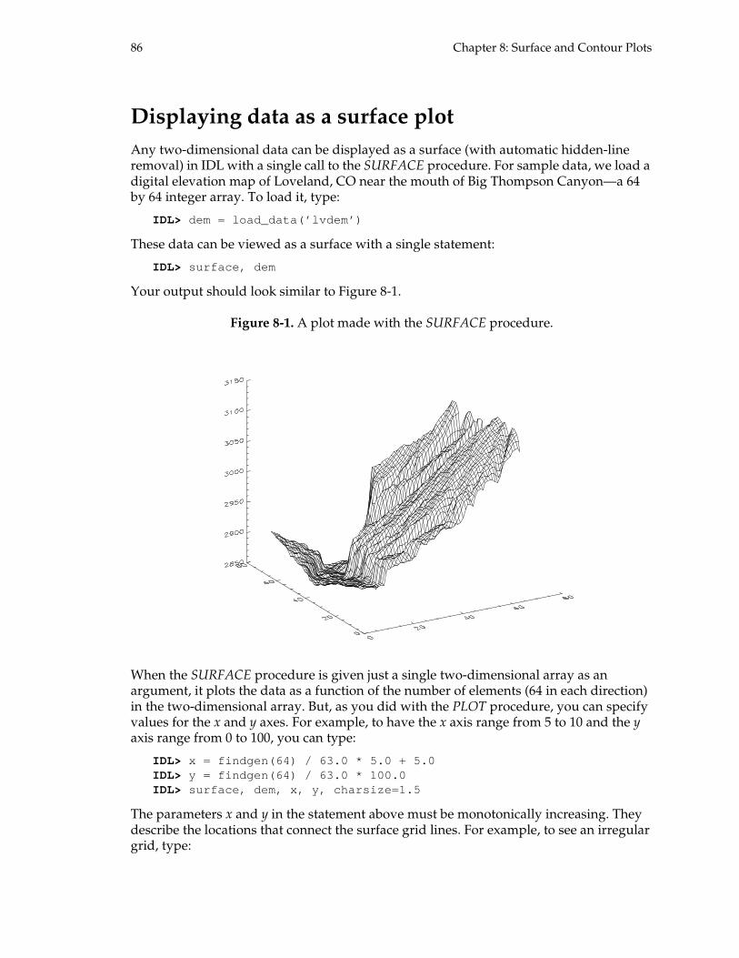
86 Chapter 8: Surface and Contour Plots
Displaying data as a surface plot
Any two-dimensional data can be displayed as a surface (with automatic hidden-line removal) in IDL with a single call to the SURFACE procedure. For sample data, we load a digital elevation map of Loveland, CO near the mouth of Big Thompson Canyon—a 64 by 64 integer array. To load it, type:
IDL> dem = load_data(’lvdem’)
These data can be viewed as a surface with a single statement:
IDL> surface, dem
Your output should look similar to Figure 8-1.
Figure 8-1. A plot made with the SURFACE procedure.
When the SURFACE procedure is given just a single two-dimensional array as an argument, it plots the data as a function of the number of elements (64 in each direction) in the two-dimensional array. But, as you did with the PLOT procedure, you can specify values for the x and y axes. For example, to have the x axis range from 5 to 10 and the y axis range from 0 to 100, you can type:
IDL> x = findgen(64) / 63.0 * 5.0 + 5.0IDL> y = findgen(64) / 63.0 * 100.0IDL> surface, dem, x, y, charsize=1.5
The parameters x and y in the statement above must be monotonically increasing. They describe the locations that connect the surface grid lines. For example, to see an irregular grid, type:

Chapter 8: Surface and Contour Plots 87
IDL> xx = [0.0, 0.1, 0.3, 2.0, 3.0]IDL> yy = indgen(5)IDL> surface, dist(5), xx, yy
The SURFACE procedure can take over 70 different keywords to modify the plot in some way, including most of the annotation keywords you learned for the PLOT procedure. For example, to add titles to the plot and to the x and y axes, type:
IDL> surface, dem, xtitle=’E <---> W’, ytitle=’N <---> S ’, $IDL> title=’Big Thompson Canyon DEM’, charsize=2.0
The plot title is rotated parallel to the axes of the surface plot. If you want the plot title to be in a plane parallel to the display screen, you may want to draw the surface with the SURFACE procedure then title it with the XYOUTS procedure. For example, type:
IDL> surface, dem, xtitle=’E <---> W’, ytitle=’N <---> S ’, $IDL> charsize=2.0IDL> xyouts, 0.5, 0.90, /normal, charsize=2.0, align=0.5 , $IDL> ’Big Thompson Canyon DEM’
Rotating a surface plot
A surface plot can be rotated about the x axis with the AX keyword and about the z axis with the AZ keyword. Rotations are expressed in degrees, oriented counterclockwise while looking toward the origin. The AZ and AX keywords default to 30 degrees if they are omitted. For example, to rotate the surface about the z axis by 50 degrees and about the x axis by 30 degrees, type:
IDL> surface, dem, az=50
To rotate about both the x axis and the z axis by 45 degrees, type:
IDL> surface, dem, az=45, ax=45
Note the effects of the rotations using AX and AZ are not cumulative. Each surface command must enter its own rotation starting from the same initial position, unless you want the default 30 degree rotation.
Adding color to a surface plot
It is easy to add color to a surface plot, using many of the same keywords that you used to add color to line plots. For example, to create a black surface plot on a white background, type:
IDL> loadct, 15IDL> surface, dem, color=0, background=255
If you want the bottom of the surface to be a different color from the top, you could use the BOTTOM keyword like this:
IDL> surface, dem, color=0, background=255, bottom=20
If you want the axes to be drawn in a different color from the surface, blue for example, you have to enter two statements:
IDL> surface, dem, color=0, background=255, bottom=20

88 Chapter 8: Surface and Contour Plots
IDL> surface, dem, /nodata, /noerase, color=100
It is also possible to draw the mesh lines of the surface in different colors. For example, you could drape a second data set over the first, coloring the mesh of the first data set with the information contained in the second data set.
To see how this would work, load a second data set and display it as a surface with these statements:
IDL> dem_image = load_data(’lvimage’)IDL> surface, dem_image
Now, drape the data in the variable dem_image over the top of the data in the variable dem, using the values of dem_image to color the mesh of dem. Do this with the SHADES keyword:
IDL> surface, dem, shades=bytscl(dem_image, top=!d.table _size-1)
Scaling the data set (with the BYTSCL function) is necessary to obtain values from the data between 0 and 255 to correspond to colors in the color table. It is not strictly necessary here because the dem_image data is already scaled.
Putting the above together with some keywords analogous to the those for the PLOT routine,
IDL> surface, dem, x, y, $IDL> shades=bytscl(dem_image, top=!d.table_size-1), $IDL> charsize=1.5, zstyle=1, zrange=[2800, 4000], $IDL> color=0, background=255
Creating shaded surface plots
It is equally easy to create a shaded surface representation of your data using the SHADE_SURF routine:
IDL> shade_surf, dem
The SHADE_SURF procedure takes most of the keywords accepted by the SURFACE procedure. For example,
IDL> shade_surf, dem, x, y, zstyle=1, zrange=[2800, 4000 ], $IDL> az=50, ax=45, charsize=2.0
Your output should look similar to Figure 8-2 on page 89.
The shading parameters used by the SHADE_SURF procedure can be changed with the SET_SHADING procedure. For example, to change the light source from the default of [0, 0, 1] to a location of [1, 1, 1] on the opposite side of the surface, type:
IDL> set_shading, light=[1, 1, 1]IDL> shade_surf, dem
Note that the syntax of the light location keyword used in SET_SHADING is light=[x,y,z] , where x, y and z are the normalized distance across, up and out of the display (or page), respectively. This location specification is independent of the view perspective which, in this case, was set in the SHADE_SURF command.

Chapter 8: Surface and Contour Plots 89
Figure 8-2. A shaded surface of the data with the surface rotated about the Z and X axes.
You can also indicate which range of values should be used from the color table (i.e., which color indices). For example, if you want to restrict the shaded surface to the blue and red range of values in color table 5, you would set the parameters like this:
IDL> set_shading, values=[0, 150]IDL> shade_surf, dem
Be sure to set the light source location and color value parameters back to their original values, or you might be confused later on in the course!
IDL> set_shading, light=[0, 0, 1], values=[0, !d.table_s ize-1]
It is also possible to drape one data set over the shaded surface by using the SHADES keyword in the same manner as was done for the SURFACE routine.
Use this data to shade the original data. Type:
IDL> shade_surf, dem, shades=bytscl(dem_image, top=!d.ta ble_size-1)
Draping another data set over a three-dimensional surface is a way to add an extra dimension to your data. For example, you just represented four-dimensional data. If you were to animate this data set over time, you would be representing five-dimensional data.
Sometimes you just want to drape the original surface on top of the shaded surface. This is easy to do by combining the SHADE_SURF and SURFACE procedures. For example, type:
IDL> shade_surf, demIDL> surface, dem, /noerase

90 Chapter 8: Surface and Contour Plots
The final plot of the previous section could also be done as a shaded surface:
IDL> shade_surf, dem, x, y, $IDL> shades=bytscl(dem_image, top=!d.table_size-1), $IDL> charsize=1.5, zstyle=1, zrange=[2800, 4000], $IDL> color=0, background=255
Displaying data with ISURFACE
The iSurface tool can provide an interactive display of the previous graphic:
IDL> tvlct, r, g, b, /getIDL> isurface, dem, texture_image=dem_image, zstyle=1, $IDL> rgb_table=[[r], [g], [b]], zrange=[2800, 4000]
With the iSurface tool, the attributes of the surface plot can be changed through the Visualization Browser, accessed by selecting Window > Visualization Browser... from the iTools Menu Bar, or by simply right-clicking on the plot and choosing “Properties” from the context menu. The visualization can be manipulated and operated upon in the standard manner of the iTools, as discussed in Chapter 5, “IDL iTools.”
Displaying data as a contour plot
Any two-dimensional data set can be displayed as a contour plot in IDL with a single call to CONTOUR:
IDL> contour, dem, x, y
Your output should look similar to Figure 8-3.
Figure 8-3. A contour plot of the dem data.

Chapter 8: Surface and Contour Plots 91
The FOLLOW keyword is used in the call to CONTOUR to display contour labels.
IDL> contour, dem, x, y, /follow
By default, IDL selects six regularly spaced contour intervals (five contour lines) to contour, but you can change this in several ways. For example, you can specify exactly how many equally spaced contour levels to draw with the NLEVELS keyword. For example, to contour your data with 10 equally spaced contours, type:
IDL> contour, dem, x, y, /follow, nlevels=10
Your output should look similar to Figure 8-4.
Figure 8-4. A contour plot with ten levels and the FOLLOW keyword set.
Additional contour lines can be added by calling CONTOUR again (perhaps more than once) with the OVERPLOT keyword set.
Sometimes you may prefer to choose the contour levels yourself, rather than have IDL calculate them. You can do this with the LEVELS keyword. The keyword is set to a vector of values where the contour levels should be drawn. For example, type:
IDL> level_values = [2900, 2920, 2940, 2960, 2980, 3000, 3050, 3100]IDL> contour, dem, x, y, /follow, levels=level_values
Notice, in this case, the contour levels are labeled automatically with their values, but that only every other contour level is labeled. You can specify exactly which contour line should be labeled with the C_LABELS keyword. This keyword is a vector with as many elements as contour lines. If the value of the element is 1 (or more precisely, if it is nonzero), the contour label is drawn; if the value of the element is 0, the contour label is not drawn. For example, to label the elevations at 100 meter intervals,
92 Chapter 8: Surface and Contour Plots
IDL> contour, dem, x, y, /follow, levels=level_values, $IDL> c_labels=[1, 0, 0, 0, 0, 1, 0, 1]
A contour plot can be customized with many of the same keywords already discussed for the PLOT and SURFACE procedures. In addition, there are a number of keywords that apply only to the CONTOUR procedure. Many of these modify the various properties of the isopleths (the lines of constant value). In Table 8-1 these type of keywords start with C_. Each keyword of this type takes a vector of the same length as the number of levels to be drawn, where each element of the vector describes the corresponding isopleth.
Displaying contours in three dimensions
Contour plots may also be projected into three dimensions. First, create a transformation matrix and put it in the system variable !p.t. Then, indicate that CONTOUR will use this transformation matrix by setting the T3D keyword.
There are several ways to specify and load a three-dimensional transformation matrix in IDL, but one of the easiest ways is to use the library routine SURFR, which creates and loads in !p.t the same three-dimensional transformation matrix used by the SURFACE and SHADE_SURF procedures. Type:
IDL> surfr, ax=25, az=45
Suppose you wanted to display a regular contour plot with a filled contour plot above it in this three-dimensional space:
IDL> contour, dem, x, y, nlevels=10, /t3d, zvalue=0.0
Table 8-1. Keywords for the CONTOUR procedure.
Keyword Description
C_ANNOTATION Set this keyword to a vector of strings for annotating the contour lines
C_CHARSIZE Sets the annotation character size
C_COLORS Sets the color index used to draw each contour
C_LABELS Specifies which contour labels to be drawn
C_LINESTYLE The line style used to draw each contour
DOWNHILL Draws tick marks on contour lines pointing "downhill"
FILL Produces a contour plot filled with solid or line-filled polygons
FOLLOW Draws labels on contour lines
LEVELS Specifies a vector containing levels to be drawn on the contour plot
MAX_VALUE Data points above this value are ignored
MIN_VALUE Data points below this value are ignored
NLEVELS Specifies the number of contour lines to be drawn
OVERPLOT Draws the contour plot over the previous contents of the window, instead of erasing the window
ZAXIS Draws a Z axis on the contour plot; the location of the z axis can be controlled by setting the value to 1, 2, 3, or 4

Chapter 8: Surface and Contour Plots 93
IDL> contour, dem, x, y, nlevels=10, /fill, /t3d, zvalue =1.0, $IDL> /noerase
If you just wanted to plot the contour lines in three-dimensional space, type:
IDL> contour, dem, x, y, nlevels=10, /t3d
This sort of representation could be combined with a color-filled display. For example:
IDL> contour, dem, x, y, nlevels=10, /t3d, /fill, zvalue =0IDL> contour, dem, x, y, nlevels=10, /t3d, /overplot
Displaying data with ICONTOUR
Contour plots can be created using the iContour tool as well,
IDL> icontour, dem
With the iContour tool, the attributes of the contour plot can be changed through the Visualization Browser, accessed by selecting Window > Visualization Browser... from the iTools Menu Bar, or by simply right-clicking on the plot and choosing “Properties” from the context menu. The visualization can be manipulated and operated upon in the standard manner of the iTools, as discussed in Chapter 5, “IDL iTools.”
Combining contour and surface plots
It is easy in IDL to combine contour and surface representations of your data. For example, to display a color-filled contour with the surface representation of the data over the top of it, type:
IDL> contour, dem, x, y, nlevels=10, /t3d, zvalue=0, /fi llIDL> contour, dem, x, y, nlevels=10, /t3d, zvalue=0, /ov erplotIDL> surface, dem, x, y, /t3d, /noerase, zstyle=1, $IDL> zrange=[2000, 3400]
Your output should look similar to Figure 8-5 on page 94.
Exercises
1. Examine the corners of your output for the combined contour/surface plot and compare it to the output in Figure 8-5. Look up the NOCLIP keyword in the online help for the CONTOUR routine and use it to fix your output.
2. Use ISURFACE to create a visualization similar to Figure 8-5.
3. Display a wire-mesh or shaded surface where color of the surface is proportional to the height of the surface. (Try this with color table #27, EOS_B.)
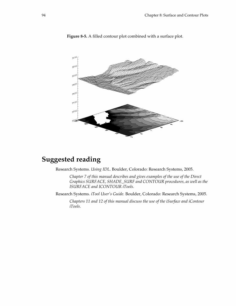
94 Chapter 8: Surface and Contour Plots
Figure 8-5. A filled contour plot combined with a surface plot.
Suggested reading
Research Systems. Using IDL. Boulder, Colorado: Research Systems, 2005.
Chapter 7 of this manual describes and gives examples of the use of the Direct Graphics SURFACE, SHADE_SURF and CONTOUR procedures, as well as the ISURFACE and ICONTOUR iTools.
Research Systems. iTool User’s Guide. Boulder, Colorado: Research Systems, 2005.
Chapters 11 and 12 of this manual discuss the use of the iSurface and iContour iTools.

95
Chapter 9:
Images
This chapter describes how to use built-in IDL routines to work with image data.
What is an image? . . . . . . . . . . . . . . . . . . . . . . 96Reading image data . . . . . . . . . . . . . . . . . . . . . 96Displaying an image . . . . . . . . . . . . . . . . . . . . 96 Scaling image data . . . . . . . . . . . . . . . . . . . . . 97 Allocating color entries with IDL . . . . . . . . 98 Requesting colors for graphics windows . . 98 Getting colors by default . . . . . . . . . . . . . . . . 99 Using multiple color tables . . . . . . . . . . . . . . 99Locating the origin of an image . . . . . . . . . . . 99Positioning an image in a window . . . . . . . 100Resizing an image . . . . . . . . . . . . . . . . . . . . . 101Reading images from the display . . . . . . . . 101 8-bit systems . . . . . . . . . . . . . . . . . . . . . . . . . 101
24-bit systems . . . . . . . . . . . . . . . . . . . . . . . 102Reading subareas . . . . . . . . . . . . . . . . . . . . . 104Working with TrueColor (24-bit) images . 104 What Is a TrueColor image? . . . . . . . . . . . 104 Displaying on 24-bit displays . . . . . . . . . . 104 Displaying on 8-bit displays . . . . . . . . . . . 105Writing or drawing on top of images . . . . 106 Dragging an object over an image . . . . . . 107 Writing or drawing on top of images . . . 108The device copy technique . . . . . . . . . . . . . 108 Erasing the box from the window . . . . . . 109Suggested reading . . . . . . . . . . . . . . . . . . . . 112

96 Chapter 9: Images
What is an image?
An image is usually thought of as a picture, but in reality any two-dimensional data can be displayed as an image. This chapter demonstrates how IDL handles and displays image data.
An image is displayed as a two-dimensional array of pixels. Since each pixel can have a value in the range of 0 to 255 (on an 8-bit display), image data are often stored as byte data.
If image arrays are not stored as byte data, they are converted to byte type with the IDL image display procedures TV and TVSCL before they are displayed.
Reading image data
Normally, images are stored in binary data files or special image file formats. In this example, we will read in a binary data file using IDL’s READU procedure. This image is a 256-by-256 byte array in the image file ctscan.dat, located in the examples/data subdirectory of the main IDL directory.
IDL> file = filepath(’ctscan.dat’, subdir=[’examples’, ’ data’])IDL> scan = read_binary(file, data_dims=[256,256])
Displaying an image
There are two Direct Graphics IDL procedures that display an image:
• TV
• TVSCL
These two procedures are identical in almost every respect, including the keywords that can be used with them. They differ in only one way: TVSCL byte scales the image data into the range of colors available on the display device before the image is displayed, whereas TV takes whatever is in the image data and puts it on the display. If the data is not already scaled into the range of 0 to 255, a window with a black color may result.
The data you just read is scaled into the range of 0 to 255. Type the following
IDL> print, max(scan), min(scan)
An 8-bit display can display colors using 256 unique color indices. This is the available “pool” of color indices used by all programs running on an 8-bit display. It is a hardware limitation. As discussed in the Color in IDL chapter, windowing systems (e.g. Windows, X, etc.) use different schemes to divide color indices among all the programs running on the display. Therefore, any one program (for example, IDL) may not have all 256 color indices available. To see how many colors are available in an IDL session, open a window on the display and print the system variable that contains the number of available color indexes:
IDL> window & print, !d.table_size
Chapter 9: Images 97
On an 8-bit display, this number is usually in the range of 210 to 240 colors, but it could be considerably less.
Now, open a window, load a color table, and display the scan image with the TV procedure:
IDL> window, 0, xsize=256, ysize=256IDL> loadct, 5IDL> tv, scan
Since the TV procedure was used, the data were just displayed without any scaling. Although it is not apparent, all the pixels with values greater than the number of colors available are set to the same color. That is, pixels with values of say 237-255 are set to the same color as pixel 236.
The difference between TVSCL and TV may be apparent if the image is also displayed with the TVSCL procedure. Open another window and move it near the first. Use TVSCL to display the image:
IDL> window, 1, xsize=256, ysize=256IDL> tvscl, scan
A slight difference in colors between the two images may be apparent.
Now, to see what TVSCL does, scale the data and display it with the TV procedure:
IDL> window, 2, xsize=256, ysize=256IDL> scaled = bytscl(scan, top=!d.table_size-1)IDL> tv, scaled
What is displayed in window 2 should be identical to what is displayed in window 1. The TVSCL procedure scales the data into the dynamic color range of the device.
The image display procedures do not erase the screen before they display the image, unlike the PLOT, SURFACE, and CONTOUR procedures. If this is a problem, issue the ERASE procedure to erase the screen before displaying the image:
IDL> erase
Scaling image data
In some situations, the colors used to display an image are critical in the interpretation of the data. In this case, the data should be scaled manually with the BYTSCL function and displayed with the TV procedure. For example, suppose that film density in CAT scans is displayed next to a color bar. The data collected this month are compared with data collected in other months by an operator of the display program. A particular shade of grey must indicate the same film density (data value) from month to month or the notes are not comparable. If this month’s and last month’s image data were displayed with the TVSCL procedure, there would be absolutely no guarantee that a particular grey color means the same thing in both data sets.
The discrepancies can arise principally from two sources. First, each IDL session may use a different number of available colors. Since TVSCL scales the image data into the number of colors in an IDL session, this could introduce errors. Second, there is no

98 Chapter 9: Images
guarantee that each data set has the same dynamic range. One outlier point would be enough to change the scaling factors and result in an inconsistent image display.
To get around these problems, scale the data with the BYTSCL function and display them with the TV procedure. To make sure the number of colors in the IDL session does not introduce errors, always scale the data into the same number of color “bins.” To make sure the range of values in the data sets does not introduce errors, scale the data into the same data range.
This is done with the keywords TOP, MIN, and MAX to the BYTSCL function. For example, suppose that data need to be displayed in 100 shades of grey (or 100 colors). Further, suppose the minimum valid value of any datum in the set is 10 and the maximum valid value of any datum in the set is 200. Use the BYTSCL function like this:
IDL> scaled = bytscl(scan, min=10, max=200, top=100)
In this example, any value less than 10 is set to 10 before the data are scaled. Similarly, any value greater than 200 is set to 200.
Display the data like this:
IDL> tv, scaled
An IDL program that uses this approach must check that there are at least 100 color indices available in the IDL session and issue an error message if not. For example:
if (!d.table_size lt 100) then $message, ’Less than 100 colors available.’
Allocating color entries with IDL
There are a number of ways IDL can work with the Motif X window manager to avoid color flashing. IDL’s request for colors is made to the X window manager at the time the first graphic window is opened from within IDL. Once the request is made and satisfied by the window manager, it cannot be changed in the current IDL session.
After the request for colors has been satisfied, the only way to change the number of colors, or the kind of color map IDL is using, is to exit IDL and start over.
Requesting colors for graphics windows
There are two ways to request colors from within IDL for a graphics window:
1. Issue a statement that displays graphic output, e.g., PLOT, SURFACE, TVSCL, etc.
2. Issue the WINDOW procedure and control the request for colors with the COLORS keyword.
Once a window has been opened in an IDL session and a color map has been set up, all IDL windows share the same color map. To see how to make it appear that there is more than one color map consult the section “Using multiple color tables” below.

Chapter 9: Images 99
Getting colors by default
IDL always requests the remaining number of colors in the shared color map. By default, when there are no remaining colors in the shared color map, IDL retrieves a private color map. When IDL is the only application running besides the window manager, IDL usually gets about 248 colors, but do not count on this.
Using multiple color tables
On an 8-bit color system, there is just one physical color table, and it is used in all IDL graphics windows. By manipulating this color table, it can appear that there are several different color tables loaded simultaneously. This is done by loading different color tables into different portions of the one physical color table. The easiest way to do this is to use the NCOLORS and BOTTOM keywords to the LOADCT or XLOADCT procedures.
For example, the image scan can be displayed in two windows that appear to use two different color tables. The trick is to scale the image data into just a portion of the color space. First, scale the image data into the range of 0 to 99:
IDL> image1 = bytscl(scan, top=99)
Now, scale the image data into the range of 100 to 199:
IDL> image2 = bytscl(scan, top=99) + 100B
Then, put the two scaled images side-by-side into the same window:
IDL> window, xsize=512, ysize=256IDL> tv, image1IDL> tv, image2, 256, 0
Now, display the image on the left with a grey-scale color table (table number 0):
IDL> loadct, 0, ncolors=100, bottom=0
Now, load some other color table for the image on the right:
IDL> xloadct, ncolors=100, bottom=100
Locating the origin of an image
When IDL displays an image, the first column and row of the image are located at the lower left corner of the image. For some images, however, the first column and row are located at the upper left corner of the image. To display images where the latter convention is used, set the system variable !order equal to one. By default, !order is set to zero. To display an image using the second convention only once, use the ORDER keyword to either the TV or TVSCL procedure. For example, to see the two conventions side-by-side, type:
IDL> window, xsize=512, ysize=256IDL> tvscl, scan, order=0IDL> tvscl, scan, order=1, 256, 0

100 Chapter 9: Images
Positioning an image in a window
When an image is displayed on screen, IDL puts the image in the lower-left corner of the window by default. Do this by specifying one parameter after the name of the image in the call to TV or TVSCL. The position is calculated from the size of the window and the size of the image (see the on-line help for the TV procedure for details). So, for example, in a 512-by-512 window, there are four positions for a 256-by-256 image, starting in the upper-left corner of the window. Try typing the following statements:
IDL> window, xsize=512, ysize=512IDL> tvscl, scan, 0IDL> tvscl, scan, 1IDL> tvscl, scan, 2IDL> tvscl, scan, 3
A pixel location can also be explicitly specified. Do this by specifying two parameters after the name of the image. For example, to locate the 256-by-256 image scan in the middle of the window we just created, type:
IDL> eraseIDL> tvscl, scan, 128, 128
In this case, the lower-left corner of the image is placed at pixel location (128,128).
For example, type the following statements to display a color bar on the left-hand side and the image on the right-hand side of a window. The display window should look similar to Figure 9-1.
Figure 9-1. An image with a color bar showing 20 color gradations.
IDL> eraseIDL> window, xsize=356, ysize=256IDL> .run IDL> for j=0,19 do beginIDL> color = (!d.table_size/20)*jIDL> tv, replicate(color, 20, 10), 40, 10*j+25
Chapter 9: Images 101
IDL> endforIDL> endIDL> tv, scan, 100, 0
The REPLICATE function creates 20-by-10 images, each filled with pixels of a particular value (in this case, the value of the variable, color)
Resizing an image
IDL provides two functions that change an image size: REBIN and CONGRID.
REBIN is limited in that the resized image must have a size that is an integral multiple or factor of the original image. For example, the image scan may be resized to 128, 512, or 1024 elements, but not to 300 or 500 elements. The image may be reduced in size in one direction and increased in size in the other dimension. For example, to resize scan to 128 columns and 512 rows:
IDL> windowIDL> new = rebin(scan, 128, 512)IDL> tvscl, new
By default, REBIN uses bilinear interpolation when magnifying, and nearest neighbor sampling when reducing. Nearest neighbor sampling can be used in both directions if the SAMPLE keyword is set. Bilinear interpolation creates better looking images but these images contain data values not present in the original array.
CONGRID is similar to REBIN, except
1. the number of columns and rows specified in the new image can be set to an arbitrary number and
2. nearest-neighbor sampling is used by default.
Set the INTERP keyword to use bilinear interpolation:
IDL> eraseIDL> new = congrid(scan, 600, 400, /interp)IDL> tvscl, new
Reading images from the display
Much time and effort can be expended building a complicated image or plot on the display device. The TVRD function, which reads the contents of the display device’s memory back into an IDL variable, can be used to save the contents of a window for display later.
8-bit systems
On a 8-bit system, TVRD reads the entire window minus the window frame and title bar into a two-dimensional byte array.
IDL> window, xsize=300, ysize=300

102 Chapter 9: Images
IDL> tvscl, scanIDL> new_image = tvrd()IDL> help, new_image
The new variable new_image is a byte array of 300 by 300 elements. The size of the window determines the size of the resulting array. The array contains the color index values of each pixel on the display.
24-bit systems
On a 24-bit system, TVRD reports different information. Each pixel in a window is represented as an RGB value internally. To correctly get a screen capture, TVRD must be used with the TRUE keyword set.
IDL> window, xsize=300, ysize=300IDL> tvscl, scanIDL> new_image = tvrd(/true)IDL> help, new_image
The variable new_image is a three-dimensional byte array (3, 300, 300). For each pixel there are three values: red, green and blue. To properly display the result, switch to decomposed mode (TrueColor) and use the TV procedure with the TRUE keyword.
IDL> device, decomposed=1IDL> tv, new_image, /trueIDL> device, decomposed=0
Common errors in 24-bit mode
The most common error using TVRD occurs on 24-bit displays. The error occurs when TVRD is called on a 24-bit system without the TRUE keyword. An example is given below.
IDL> window, /free, xsize=300, ysize=300IDL> tvscl, scan IDL> img_capture = tvrd()IDL> help, img_capture
On 8 and 24-bit systems the result of the command is a 300 by 300 byte array; however, the contents of the array are different. On an 8-bit system the array contains color index values that produce the correct image. On a 24-bit machine the array contains an array of maximum intensity values. IDL reads the RGB triples at every pixel and returns R, G or B, whichever has the greatest value, in the array. When the resulting image is viewed using TV or TVSCL, the colors are incorrect. An example of what happens when an 8-bit capture is used on a 24-bit system is given in Figure 9-2.

Chapter 9: Images 103
Figure 9-2. The result of capturing a window using TVRD on a 24-bit display. The middle window was captured with new_image=tvrd(). The right window was captured with
new_image=tvrd(/TRUE)
The suggested method of using TVRD to read and display images on 8 and 24-bit displays is to use a simple conditional statement.
IDL> device, get_visual_depth=vdIDL> new_image = tvrd(true=(vd gt 8))
The visual display depth of the system is obtained from the DEVICE procedure and stored in the variable vd. The call to TVRD is made with the TRUE keyword set to a logical statement. When the visual depth is greater than 8 bits, TRUE is set, if not, TRUE is not set.
Printing 24-bit image captures
One of the common uses of TVRD is to capture graphics and annotations on the screen and send them to a printer. Printing is covered in a later chapter but the process is laid out here. The printer and PostScript devices in IDL are 8-bit devices and cannot render 24-bit images. When a proper screen capture is performed on a 24-bit system, the resulting image is 24-bit. To render the 24-bit image to the printer, the image must be scaled down to 8 bits using the COLOR_QUAN function.
IDL> device, get_visual_depth=vdIDL> new_image = tvrd(true=(vd gt 8))IDL> olddev = !d.nameIDL> set_plot, ’Printer’IDL> if (vd gt 8) then new_image = color_quan(new_image, 1, r, g, b)IDL> if (vd gt 8) then tvlct, r, g, bIDL> tv, new_image, xsize=6, ysize=6, /inchesIDL> device, /close_documentIDL> set_plot, olddev
The statements above use TVRD to capture the image, switch to the printer device, color quantize the image only when the display depth is greater than 8 bits and draw the image. See Chapter 15, “Graphics Devices” for more information about output to graphics devices such as printers and PostScript.

104 Chapter 9: Images
Reading subareas
A portion of the window can be also saved by specifying the pixel coordinates of the lower left corner of the part of the window and the number of columns and rows to read. For example, to start at pixel location (100, 75) and read 150 columns and 80 rows, type:
IDL> device, get_visual_depth=vdIDL> new_image = tvrd(100, 75, 150, 80)
The image obtained from reading the display device can be treated just like any other image in IDL. To display it, type:
IDL> eraseIDL> tv, new_image
The TVRD function is often used to save a complicated and annotated image so that it can be output later in hardcopy or used in an image series presentation.
Working with TrueColor (24-bit) images
So far, the discussion has assumed 8-bit images (two-dimensional byte data arrays). It is becoming more common to encounter TrueColor (24-bit) images.
In general, when working with images, these factors must be considered:
• The number of simultaneously displayable colors of the display (the color depth)
• Image type (8-bit, 24-bit, etc.)
• The type of pixel interleaving of the image
What Is a TrueColor image?
A 24-bit image is always a three-dimensional data set, with one of its dimensions set to three. For example, the data could be an m-by-n-by-3 array, in which case the image is said to be band-interleaved. If the image is m-by-3-by-n it is said to be row-interleaved, and if it is 3-by-m-by-n it is said to be pixel-interleaved. The type of interleaving used is based on data access considerations (speed and/or ease of access). When displaying a TrueColor image, the color that a pixel on the display attains is the result of “mixing” the red, green and blue values originating as three data elements in the data. These data elements range in value from 0 to 255. Notice that all of the information regarding color is contained in the 24-bit data set.
In contrast, an 8-bit image exists as a single two-dimensional byte array. On an 8-bit display, the data elements of the array are used to access three color vectors internal to IDL. Recall that these vectors can be copied into variables with the statement:
IDL> tvlct, red, green, blue, /get
Displaying on 24-bit displays
Displaying TrueColor images on a 24-bit display is quite easy: TrueColor images can be displayed with the TV procedure. To display a 24-bit image on a 24-bit display, use the

Chapter 9: Images 105
TRUE keyword to indicate what kind of interleaving is being used. TRUE=1 means pixel-interleaved, TRUE=2 means row-interleaved and TRUE=3 means band-interleaved. For example, to display a pixel-interleaved 24-bit image the following statement would be used:
IDL> tv, image_array, true=1
Displaying on 8-bit displays
To display TrueColor images on an 8-bit display, the COLOR_QUAN function is used. The COLOR_QUAN function quantizes a TrueColor image and returns an 8-bit image and palette to display the image on a standard 8-bit display. The output image and palette can have from 2 to 256 colors. This means images using more than 256 colors will have some error associated with this method. Use COLOR_QUAN’s ERROR keyword to quantify this error.
COLOR_QUAN solves the general problem of accurately displaying TrueColor images on displays that can only display 256 (or fewer) simultaneous colors. The way COLOR_QUAN is called depends on the type of TrueColor image. If the image were composed of three two-dimensional arrays (one for red, green and blue), then the calling sequence would be:
IDL> result = color_quan(image_r, image_g, image_b, r, g , b)
If the image exists as a 3-dimensional array, COLOR_QUAN is called as follows:
IDL> result = color_quan(image, dim, r, g, b)
where the second positional parameter dim, specifies the type of interleaving. A value of 1 indicates interleaving by pixel, (3, n, m) , a value of 2 indicates interleaving by row, (n, 3, m) , and a value of 3 indicates interleaving by band, (n, m, 3) —just as in the table above.
The parameters r, g and b contain the red, green, and blue components of the output palette to be loaded into the color table with TVLCT. For example:
IDL> file = filepath(subdir=[’examples’,’data’], ’rose.j pg’)IDL> read_jpeg, file, image_24bitIDL> image_8bit = color_quan(image_24bit, 1, r, g, b)IDL> tvlct, r, g, bIDL> window, xsize=227, ysize=149IDL> tv, image_8bit
Table 9-1. TrueColor image organization.
Interleaved by… Array dimensions AbbreviationTRUE keyword
value
pixel 3, m, n BIP 1
row m, 3, n BIL 2
band m, n, 3 BSQ 3

106 Chapter 9: Images
Writing or drawing on top of images
Quite often in IDL, you would like to be able to write or draw on top of an image. For example, you might want to write some type of annotation or you might want to draw some type of region of interest on your image.
Most window devices allow you to specify a graphics function. Table 9-2 gives a list of graphics functions available in the IDL Direct Graphics system.
The graphics function is a logical function that specifies how the pixel values of an object interact with the pixel values that are already on the display screen. The default graphics function is Copy (index 3). This means that the pixel values of the new object completely overwrite the pixel values that already exist on the display.
One way to write information on top of an image is to set the graphics function to exclusive OR or XOR mode (index 6). You set the graphics function with the DEVICE procedure and the SET_GRAPHICS_FUNCTION keyword. First display an image. Then set the graphics function to XOR, by typing:
IDL> tvscl, scanIDL> device, set_graphics_function=6
Next, look at the picture of the box in Figure 9-3. Create two vectors, xbox and ybox, that describe the x and y coordinates, respectively, of the corners of the box. Draw the box on top of the image with the PLOTS procedure by typing:
IDL> xbox = [0.2, 0.2, 0.8, 0.8, 0.2]IDL> ybox = [0.2, 0.8, 0.8, 0.2, 0.2]IDL> plots, xbox, ybox, /normal
Table 9-2. The possible graphics functions available with IDL.
Index Graphical Function Definition
0 GX 0
1 GXand source AND destination
2 GXandReverse source AND (NOT destination)
3 GXcopy (default) source
4 GXandInverted (NOT source) AND destination
5 GXnoop destination
6 GXxor source XOR destination
7 GXor source OR destination
8 GXnor (NOT source) AND (NOT destination
9 GXequiv (NOT source) XOR destination
10 GXinvert (NOT destination)
11 GXorReverse source OR (NOT destination)
12 GXcopyInverted (NOT source)
13 GXorInverted (NOT source) OR destination
14 GXnand (NOT source) OR (NOT destination)

Chapter 9: Images 107
Figure 9-3. The coordinates of the corners of a box in normalized coordinate space.
Notice, that the outline of the box is not drawn in a single color. Rather, it is drawn in the “opposite” color of each underlying pixel, since the XOR mode “flips” the individual bits in the pixel value that is currently displayed on the screen (when drawing with color index 255).
To erase the box, “flip” the individual bits of the pixel values back to their original settings by typing the PLOTS procedure again:
IDL> plots, xbox, ybox, /normal
Be sure to set the graphics function back to the original Copy (index 3) by typing:
IDL> device, set_graphics_function=3
Dragging an object over an image
You can combine the CURSOR procedure with the ability to control the graphics function to move or drag an object around the display screen. Here is a routine that allows you to move a text string around the display window until you click the right mouse button. This code is in the file name move.pro; you do not need to type these lines.
window, 0, xsize=256, ysize=256tvscl, scan!err = 0device, set_graphics_function=6wshow, 0 cursor, x1, y1, /device, /downxyouts, x1, y1, /device, ’HELLO’, charsize=3, align =0.5while (!err ne 4) do begin
cursor, x2, y2, /device, /nowaitxyouts, x1, y1, /device, ’HELLO’, charsize=3, align =0.5xyouts, x2, y2, /device, ’HELLO’, charsize=3, align =0.5x1 = x2y1 = y2
endwhiledevice, set_graphics_function=3
(0.2, 0.8) (0.8, 0.8)
(0.2, 0.2) (0.8, 0.2)

108 Chapter 9: Images
end
Enter the following line to run this main-level IDL program.
IDL> .run move.pro
Move the cursor around in the window you just created. Notice how the text string follows the cursor about the window. To exit this program, you must click the right mouse button!
The device copy technique
Although the program above works, the fact is you cannot specify that you want the word ‘HELLO’ to be drawn in, say, yellow. So there is another important technique that IDL programmers use to write or draw on top of an image. This technique uses pixmap windows and is called the Device Copy technique.
A pixmap is an IDL graphics window. But it does not exist on the display as normal IDL graphics windows do. Instead, it exists in memory. Everything you can do in a normal IDL graphics window, you can also do in a pixmap window. Create a pixmap window using the WINDOW procedure and the PIXMAP keyword, like this:
IDL> window, 1, xsize=256, ysize=256, /pixmap
Notice that window 1 is not on your display. If you had a window with window index 1 on the display, it would have been destroyed and recreated as a pixmap when you executed the statement above.
To put something in this pixmap window, you issue the IDL graphics statement you would use to put something in a IDL graphics window. For example to display the image data you loaded earlier, you can type:
IDL> tv, scan
Notice that there is still nothing visible on your display. This statement has been executed and the image displayed on the pixmap window in memory.
You can make this pixmap window the current graphics window and delete it the same as normal IDL windows:
IDL> wset, 1IDL> wdelete, 1
Writing or drawing on top of images
Quite often in IDL, you would like to write or draw on top of an image or some other graphic display. For example, you might want to write an annotation or draw a region of interest polygon on your image.
To set this up properly, type the following statements that load a grayscale color table, create a window, and display the image you loaded earlier. Notice that you are scaling the image data into the first 200 colors of the color table. Type:
IDL> loadct, 0

Chapter 9: Images 109
IDL> window, 0, xsize=256, ysize=256IDL> tv, bytscl(scan, top=199)
Suppose you would like to draw a box on top of this image in a yellow color. You see the device coordinates of such a box in Figure 9-4. You can use the PLOTS procedure to draw such a box on the image, providing you create a vector of x coordinates and a vector of y coordinates. If you start at the lower left corner of the box and traverse clockwise, the coordinates can be described like this. The last coordinate pair complete the box.
IDL> box_xcoord = [80, 80, 160, 160, 80]IDL> box_ycoord = [75, 175, 175, 75, 75]
To draw this box on your image in yellow, load the triple (255, 255, 0) into the color table at color index 200, then use the PLOTS procedure to draw the box. Type:
IDL> tvlct, 255, 255, 0, 200IDL> plots, box_xcoord, box_ycoord, /device, color=200
Figure 9-4. The coordinates of a box that will be drawn on top of an image.
Erasing the box from the window
The question now arises, how do you erase the box from the display? Well, you could, of course, just redisplay the image in the window. This certainly “erases” the box. But as you will see, you are going to want to do this erasure in a loop and re-displaying the image is going to be much too slow for your purposes.
A much, much faster technique uses a pixmap and the Device Copy technique. This technique is a factor of 10 to 100 times faster than just re-displaying the image. To create a pixmap for erasing the window, you create a pixmap that is the same size as the display window, and load the pixmap window with the same image data that is in the display window, without the box drawn on it, of course! Type:
IDL> window, 1, xsize=256, ysize=256, /pixmapIDL> tv, bytscl(scan, top=199)

110 Chapter 9: Images
Since the pixmap window is now the current graphics window, make the display window (window index number 0) the current window by typing:
IDL> wset, 0
The device copy technique allows you to copy a rectangular portion of a “source window” into a “destination” window. You see an illustration of the technique in Figure 9-5. In the device copy technique, a rectangular area in the source window is copied to the destination window. The COPY keyword requires the coordinates of the lower left corner of the copy rectangle in the source window, the number of columns and rows to copy, the coordinates of the lower left corner of the copy rectangle in the destination window, and the window index number of the source window. The copy is always made from the source window to the current graphics window. The source window and the destination window can be the same window.
Figure 9-5. Illustration of source and destination windows for the device copy technique.
The general form of the device copy technique is:
device, copy=[sx, sy, width, height, dx, dy, source ID]
where the elements of the copy keyword are given in Table 9-3.
You will be using the device copy technique to copy the entire source window (which is the pixmap window, window index 1) into the destination window (which is the display window, window index 0), thereby erasing the box that you just drew on the image. In other words, the copy rectangle will start at (0, 0) and will include as many columns and rows as the pixmap window is wide and tall. The copy rectangle will be the entire pixmap window, located at (0, 0) in the destination window. Type:
IDL> device, copy=[0, 0, 256, 256, 0, 0, 1]
While the technique of copying the entire pixmap window into the display window is usually fast enough for most applications, it is even faster to copy just the portion of the display window that needs to be “repaired.” In this case, the portion that needs to be
Source Destination
(sx, sy)
width
heig
ht
(dx, dy)
Source Destination
(sx, sy)
width
heig
ht
(dx, dy)

Chapter 9: Images 111
repaired is just the pixels underneath the lines that comprise the box. To put the box back on your image, type:
IDL> plots, box_xcoord, box_ycoord, /device, color=200
To repair the two vertical lines of the box, type:
IDL> device, copy=[80, 75, 1, 101, 80, 75, 1]IDL> device, copy=[160, 75, 1, 101, 160, 75, 1]
To repair the two horizontal lines of the box, type:
IDL> device, copy=[80, 75, 81, 1, 80, 75, 1]IDL> device, copy=[80, 175, 81, 1, 80, 175, 1]
Now the MOVE program above can be rewritten to use pixmaps and the device copy technique rather than the XOR graphics function. This program is saved in the introduction directory as movepix.pro; you do not need to type it.
window, 0, xsize=256, ysize=256tv, bytscl(scan, top=199)!err = 0window, 1, xsize=256, ysize=256, /pixmaptv, bytscl(scan, top=199)wset, 0wshow, 0 tvlct, 255, 255, 0, 200cursor, x1, y1, /device, /downxyouts, x1, y1, /device, ’HELLO’, charsize=3, $
align=0.5, color=200while (!err ne 4) do begin
cursor, x2, y2, /device, /nowaitdevice, copy=[0, 0, 256, 256, 0, 0, 1]xyouts, x2, y2, /device, ’HELLO’, charsize=3, $
Table 9-3. Description of the array parameter for the COPY keyword of the DEVICE procedure.
Parameter Description
sx and sy are the device coordinates of the lower left corner of a copy rectangle in the source window (the window you are copying from)
width indicates the number of columns to copy
height indicates the number of rows to copy
dx and dy are the device coordinates of the lower left corner of the copy rectangle in the destination window
sourceID is the window index number of the source window. You always copy from the window specified with this window index number to the current graphics window, the window specified in the system variable !D.Window. The window you are copying from and the current graphics window can be, and often are, the same window

112 Chapter 9: Images
align=0.5, color=200endwhilewdelete, 1end
To run this IDL program type
IDL> movepix
Move the cursor around in the window you just created. The text string follows the cursor about the window. The word ‘HELLO’ is now always drawn in yellow. To exit this program, click the right mouse button.
Suggested reading
Research Systems. Getting Started with IDL. Boulder, Colorado: Research Systems, 2005.
This document gives many tutorial-like examples of using IDL that are suitable for new users. From the Contents tab of the IDL Online Help utility, select User’s Guides > Getting Started with IDL.
Research Systems. iTool User’s Guide. Boulder, Colorado: Research Systems, 2005.
An explanation of how to use the new IDL iTools, along with many examples. This document can be accessed in the same manner as Getting Started with IDL, described above.

113
Chapter 10:
Programming
This chapter describes the building blocks for creating and calling IDL programs.
If you need more than 3 levels of indentation, you’re screwed anyway, and should fix your program.
—Linus Torvalds (from http://en.wikiquote.org )
Operators . . . . . . . . . . . . . . . . . . . . . . . . . . . . . 114 Matrix multiplication . . . . . . . . . . . . . . . . . . 116 Array operations . . . . . . . . . . . . . . . . . . . . . 116 Compound operators . . . . . . . . . . . . . . . . . . 117Control statements . . . . . . . . . . . . . . . . . . . . . 117 Compound statements . . . . . . . . . . . . . . . . 118 Conditional statements . . . . . . . . . . . . . . . . 118 Loop statements . . . . . . . . . . . . . . . . . . . . . . 119 Jump statements . . . . . . . . . . . . . . . . . . . . . . 120
The definition of true and false . . . . . . . . . 120Procedures and functions . . . . . . . . . . . . . . 121 System and user routines . . . . . . . . . . . . . . 121 Parameter passing . . . . . . . . . . . . . . . . . . . . 121 Calling programs . . . . . . . . . . . . . . . . . . . . 122Documentation . . . . . . . . . . . . . . . . . . . . . . . 123Exercises . . . . . . . . . . . . . . . . . . . . . . . . . . . . . 124Suggested reading . . . . . . . . . . . . . . . . . . . . 124

114 Chapter 10: Programming
The Interactive Data Language
IDL is an interpreted, fourth-generation computer language, built on ANSI C. Much of IDL’s utility stems from its ability to be used as an ad hoc analysis tool. However, IDL is also a robust programming language, with many of the same tools found in other modern programming languages. With IDL, a user can build complex and efficient analysis programs (as in C or FORTRAN) or user interfaces (as in Java or Visual Basic).
In this chapter, we discuss the programming components available in IDL and how to apply them correctly. For a more complete treatment of the topics in this chapter, refer to the reference document Building IDL Applications, available through IDL Online Help.
Operators
Operators are programming elements used to combine values, variables and expressions into more complex expressions or statements. Table 10-1 shows the operators IDL supports, their precedence, and gives examples of their use. More information on operators, as well as examples of using them, can be found in the Online Help.
Table 10-1. Operators and operator precedence.
Priority Operator Description Example
Highest ( ) parentheses for grouping
IDL> print, 3*2+1, 3*(2+1)7 9
[ ] brackets for concatenating arrays
IDL> a = indgen(3)IDL> print, [a, -17]
0 1 2 -17
( ) parentheses in a function call
IDL> print, indgen(3)*20 2 4
[ ] brackets for subscripting arrays
IDL> a = findgen(5)IDL> print, a[3]*2
6
. structure dereference IDL> s = {val:5}IDL> print, s.val*2
10
* pointer dereference IDL> p = ptr_new(1)IDL> print, *p
1
++ increment IDL> a = 5IDL> print, a++, a, ++a
5 7 7
-- decrement IDL> print, a--, a, --a7 5 5
^ exponentiation IDL> a = 5.0IDL> print, a^2, a^(-2)
25.0000 0.0400000

Chapter 10: Programming 115
# and ## matrix multiplication (see “Matrix multiplication” below)
* multiplication IDL> print, 5*210
/ division IDL> print, 5/2, 5/2.2 2.50000
mod modulo IDL> print, 5 mod 21
+ addition / string concatenation
IDL> print, 5+27
IDL> print, ’Dave’ + ’Stern’DaveStern
- subtraction / unary negation
IDL> print, 5-2, -53 -5
< minimum IDL> print, 5 < 22
> maximum IDL> print, 5 > 25
not bitwise complement IDL> print, not 5-6
eq equal to IDL> print, 5 eq 2, 2.0 eq 20 1
ne not equal to IDL> print, 5 ne 2, 2.0 ne 21 0
le less than or equal to IDL> print, 5 le 2, 2.0 le 20 1
lt less than IDL> print, 5 lt 2, 2.0 lt 20 0
ge greater than or equal to
IDL> print, 5 ge 2, 2.0 ge 21 1
gt greater than IDL> print, 5 gt 2, 2.0 gt 21 0
and bitwise and IDL> print, 5 and 64
or bitwise or IDL> print, 5 or 67
xor bitwise exclusive or IDL> print, 5 xor 63
Table 10-1. Operators and operator precedence.
Priority Operator Description Example

116 Chapter 10: Programming
When operators of the same level of precedence are used without grouping in an expression, they are evaluated from left to right. For example:
IDL> print, 5 mod 2 * 33
Matrix multiplication
The # operator computes an array product by multiplying the columns of the first array by the rows of the second. The ## operator computes an array product by multiplying the rows of the first array by the columns of the second. The latter operation is equivalent to mathematical matrix multiplication.
For example:
IDL> a = indgen(3,2) ; 3 x 2 array, in IDL syntaxIDL> print, a
0 1 23 4 5
IDL> b = indgen(2,3) ; 2 x 3 arrayIDL> print, b
0 12 34 5
IDL> print, a # b3 4 59 14 1915 24 33
IDL> print, a ## b10 1328 40
Note that for arrays x and y of compatible dimensions, x ## y = y # x .
Array operations
IDL operators can be used with arrays as well as with scalars. For example:
IDL> print, indgen(5) mod 20 1 0 1 0
&& logical and IDL> print, 5 && 61
|| logical or IDL> print, 5 || 61
~ logical negation IDL> print, ~50
Lowest ? : ternary (conditional expression)
IDL> y = (x gt 0) ? x : -x
Table 10-1. Operators and operator precedence.
Priority Operator Description Example

Chapter 10: Programming 117
Here, the modulo operator MOD is applied to each element of the return from the INDGEN function. Other examples:
IDL> print, indgen(5) > 22 2 2 3 4
IDL> print, indgen(5) gt 20 0 0 1 1
In each case, the operator is applied on an element-by-element basis to the array.
Compound operators
Starting with version 6.0, compound operators are supported in IDL. The available operators are listed in Table 10-2.
These compound operators combine assignment with another operator. A statement such as
a op= expression
is equivalent to
a = temporary(a) op expression
where op is an operator that can be combined with assignment to form one of the operators listed in Table 10-2, and expression is an IDL expression. For example:
IDL> a = 3IDL> a += 5 * !piIDL> print, a
18.7080
The final value of a is its initial value plus the quantity 5π.
Control statements
IDL has a complete set of control statements. These statements are logically equivalent to control statements in other programming languages. They often have similar, if not identical, syntax.
A list of control statements, with examples of their use, is provided in the following subsections.
Table 10-2. Compound operators.
*= /= += -= #=
##= <= >= and= or=
xor= ^= eq= ne= lt=
le= gt= ge= mod=

118 Chapter 10: Programming
Compound statements
By default, a control statement in IDL is a single execution step. Several execution steps can result from a control statement when they are grouped in a BEGIN-END block. This is called a compound statement. For example, this IF-THEN control statement
if (x lt 0) then print, x
does not need a BEGIN-END block, whereas this statement
if (x lt 0) then beginprint, xy = -x
endif
does.
In this example, the END statement takes the form ENDIF. END is sufficient to close any BEGIN block, but ENDIF makes the code easier to read, which is desirable. Each control statement in IDL has its own version of END. Note that BEGIN and END are reserved keywords in IDL, so you can’t use them as variable or program names.
Conditional statements
Conditional statements are used to give different results for different inputs.
if-then-else
The IF statement is used to conditionally execute a statement or a block of statements. Examples:
x = randomu(seed, 1) - 0.5if (x gt 0) then print, xif (x gt 0) then y = x else y = -xif (x gt 0) then begin
y = xendif else begin
y = -xendelse
The parentheses around the conditional are not necessary, but they improve the readability of the code. See also “The definition of true and false” on page 120 for information on evaluating conditionals.
case
The CASE statement is used to select one statement (which may be compound) for execution, depending upon the value of the case selector expression.
case piechoice of0: begin
pie = ’apple’topping = ’ice cream’end
1: pie = ’pumpkin’
Chapter 10: Programming 119
else: pie = ’cherry’endcase
The ELSE clause is optional, but note that it requires a colon, unlike the ELSE clause in an IF statement. If an expression evaluates to a value not explicitly stated in CASE, and there is no ELSE, an error results.
switch
The SWITCH statement is used to select one or more statements (which may be compound) for execution, depending upon the value of the switch selector expression. SWITCH differs from CASE in that if a match is found, subsequent items in the list are executed, until an ENDSWITCH or a BREAK statement (see “Jump statements” below) is found.
x = randomn(seed)switch 1 ofx lt 0: begin
print, ’x is less than zero’break
endx gt 0: print, ’x is greater than zero’x eq 0: print, ’x is equal to zero’else:endswitch
Note that if x is greater than zero, the last two statements in the SWITCH body are executed, as is the ELSE.
Loop statements
A common programming task is to execute a statement, or a set of statements, multiple times.
for-do
The FOR loop executes a statement or block of statements a specified number of times.
for j=0, 9 do print, j
It is possible to specify the magnitude of loop counter, as well as its direction. For example, in the following program code the loop counter is decremented by two on each iteration of the loop.
sequence = findgen(21)for j=20, 0, -2 do begin
print, j, sequence[j], sequence[j] mod 4endfor
while-do
The WHILE loop executes a statement or block of statements as long as its test condition is true. The condition is checked at the entry point of the loop.
previous = 1 & current = 1while (current lt 100) do begin

120 Chapter 10: Programming
next = current + previousprevious = currentcurrent = next
endwhile
This code generates a Fibonacci sequence: 1, 1, 2, 3, 5, 8, 13, ...
repeat-until
The REPEAT-UNTIL loop is similar to WHILE, except that the condition is tested at the exit point of the loop.
repeat begin n++
endrep until (n gt 20)
Jump statements
break
The BREAK statement provides a convenient way to immediately exit from a FOR, WHILE, REPEAT, CASE, or SWITCH statement
continue
The CONTINUE statement provides a convenient way to immediately start the next iteration of the enclosing FOR, WHILE, or REPEAT loop. Whereas the BREAK statement exits from a loop, the CONTINUE statement exits only from the current loop iteration, proceeding immediately to the next iteration.
The definition of true and false
What is true and what is not, for the different IDL data types, is listed in Table 10-3.
In a program unit, if the LOGICAL_PREDICATE option is set for the COMPILE_OPT statement, the rules given in Table 10-3 change to those displayed in Table 10-4.
Table 10-3. The definition of truth, in IDL.
Variable or expression type Truth statement
Integer (byte, integer, long) odd values are true, even values are false
Floating point (float, double, complex)
nonzero values are true, zero values are false; the imaginary part of a complex number is ignored
String nonzero lengths are true, null strings are false
Heap variable (pointers, objects) valid heap variable data are true, null heap variable data are false
Table 10-4. The definition of truth, with LOGICAL_PREDICATE.
Variable or expression type Truth statement
Numeric nonzero values are true, zero is false
String and heap variable non-null values are true, null values are false

Chapter 10: Programming 121
For more information on the COMPILE_OPT statement, check the Online Help.
Procedures and functions
Procedures and functions are self-contained modules that break large tasks into smaller, more manageable ones. Modular programs simplify debugging and maintenance and, because they are reusable, they minimize the amount of new code required for each application.
The basics of defining IDL procedures and functions are discussed in Chapter 3, “IDL Basics.” In this section, we present some important details for working with procedures and functions.
System and user routines
Many of the routines in the IDL distribution are written in C, while the rest are written in the IDL language itself. The IDL routines written in C are commonly called system or core routines. They include such routines as PRINT, HELP, PLOT, SURFACE, CONTOUR and TV. They are stored in shared libraries in the bin subdirectory of the IDL distribution. The IDL routines written in the IDL language are called user routines. They are stored in individual files listed in the lib subdirectory of the IDL distribution. They include such routines as LOADCT, FILEPATH and CONGRID, as well as the IDL iTools.
The IDL programs we create are user routines. User routines are stored in files. Multiple routines can be stored in the same file. Unlike system routines, user routines must be compiled. A file containing a user routine should be listed in a directory in IDL’s path; otherwise, it must be explicitly compiled for its contents to be accessible to IDL. (See “Calling programs” below and Chapter 3, “IDL Basics” for more information on path.)
Parameter passing
Positional and keyword parameters are used to pass information from one program to another in IDL. Almost every IDL program uses parameters. This section describes the two distinct mechanisms by which parameters are passed.
Examine the difference between the arguments used in these two calls to the PLOT procedure:
IDL> x = findgen(10)IDL> plot, x ; First callIDL> plot, findgen(10) ; Second call
Both calls get the same data and produce the same result—a plot of a line from zero to nine. The difference lies in the way the data are passed to PLOT: a variable is passed in the first call, an expression (the return from a function call) in the second.
Two parameter passing mechanisms exist in IDL: pass by value and pass by reference. Pass by value means that each parameter gets a copy of its argument's value, so that changes to the parameter do not affect the argument, even if the variables are the same name, and changes are lost when the program returns. By default, C and Java use pass by value. With pass by reference, an argument is not copied to its parameter. Any modifications to

122 Chapter 10: Programming
the parameter in the program change the argument because the two reference the same memory. By default, FORTRAN uses pass by reference.
Why is this distinction important? Many IDL routines use parameters to pass information back to a caller. Take, for example, this call to the WHERE function:
IDL> index = where(x lt 5, count)
The second argument in WHERE is used to return the number of times the conditional expression in the first argument is matched. This argument needs to be passed by reference, or information cannot be returned.
The rules for determining how a parameter is passed in IDL are:
• Expressions, including subscripted array elements, structure fields, system variables and constants are passed by value.
• Named variables are passed by reference.
The pass by reference mechanism makes it possible for information in a variable to be modified when it is passed to a program. Be aware that inadvertently modifying the contents of a parameter passed by reference will change the value of the argument at the calling level!
Calling programs
IDL’s calling mechanism is a series of steps that locate, resolve and execute a procedure or function, when the procedure or function is called by name, either from the command line or from within an IDL program. For example, when calling the procedure LOADCT from the command line:
IDL> loadct, 5% Compiled module: LOADCT.% Compiled module: FILEPATH.% Compiled module: PATH_SEP.% LOADCT: Loading table STD GAMMA-II
The calling mechanism is used to locate, resolve and execute LOADCT, loading color table 5 into an IDL session.
The calling mechanism consists of four steps.
1. Look for the named routine in IDL’s table of system routines. If the routine is listed in the system table, execute it; otherwise, proceed to the next step.
2. Check whether the routine exists in a compiled state in the current IDL session. This can be diagnosed by calling HELP with the ROUTINES keyword set. If the program is already compiled, then run it. If not, then fall to the next step.
3. Search for a file on the file system that has the same basename as the called routine, with a .pro or .sav extension. The search starts in the current IDL directory, then proceeds through the directories listed in the !path system variable. If the file is found, IDL compiles any program units it encounters in the file, starting at the top, until the called routine is found. The called routine

Chapter 10: Programming 123
is then compiled and executed. If a file with the same name as the called routine is not found, or if a file with the same name is found, but it doesn’t contain the called routine, then fall to the last step.
4. Issue an error message, stating that the requested procedure or function cannot be found.
In the above example of calling LOADCT, step 3 was reached in the calling mechanism. LOADCT is not a system routine, nor was it compiled earlier. However, the file loadct.pro exists in the lib subdirectory, which is a part of IDL’s default search path. IDL opened the file, compiled the procedure LOADCT within and executed it.
Note that the FILEPATH and PATH_SEP routines were also resolved in the call to LOADCT. These routines are called from inside the LOADCT program; therefore, they are also resolved and executed by IDL’s calling mechanism!
Step 2 improves IDL’s efficiency. If a routine has already been compiled (which means it exists in memory), it is quicker to use it than searching the path for a file and compiling the contents of that file. This has a side effect in that when debugging, any changes to a program need to be explicitly compiled; otherwise, IDL simply uses the compiled version of the routine.
Documentation
Documentation is used by programmers to help the reader of a program understand what it does.
A standard template for IDL documentation is provided in the file template.pro in the examples subdirectory. This template is used by RSI engineers when they write new IDL routines. Examine this file in the IDLDE by using the .edit executive command:
IDL> .edit template
A complete explanation of a program can be entered by a programmer into the header area at the top of this file. Note that the characters "+" and "-" bracket the header information; also, each line in the header is prefixed with ";", the IDL comment symbol. These characters are flags used by the documentation programs that are a part of the IDL distribution.
One documentation program is DOC_LIBRARY. DOC_LIBRARY reads the header information between the "+" and "-" in a program file and prints it in the output log. For example, to view the header for the program LOADCT, type
IDL> doc_library, ’loadct’
A second documentation program available in IDL is MK_HTML_HELP. The MK_HTML_HELP procedure, given a list of .pro files, or the names of directories containing such files, generates a single HTML file that contains the standard IDL documentation headers for these routines. The resulting file can be viewed with a web browser. For example, to view the documentation for the IDL programs in the course directory, type:

124 Chapter 10: Programming
IDL> mk_html_help, get_intro_dir(), ’course_files.html’
To view the results, open the file course_files.html in the browser of your choice.
IDLdoc is a hypertext documentation system for IDL code, akin to javadoc for java source code. It is intended to show the API of a code library in an easy-to-browse manner. It produces HTML pages—one page per .pro file, as well as a directory listing, overview pages, and an index of files, routines, keywords, and parameter names. IDLdoc is not a part of the IDL distribution. Instead, it’s found on RSI’s Codebank (http://www.rsinc.com/codebank ; search for IDLdoc).
The course files for this class have been IDLdoc’ed. Open the file index.html in the introduction directory to see an example of how IDLdoc’ed code appears. Check the comments in the source .pro files in introduction and compare them to their IDLdoc’ed output.
Exercises
1. Write a function to return the mean of an array of numbers. (But doesn’t IDL have a MEAN function? How can you ensure your mean function is used?)
2. Build a function that returns an ordered set of prime numbers, given the number of primes desired as user input.
Suggested reading
Gumley, Liam E. Practical IDL Programming. San Francisco: Morgan Kaufmann, 2001.
An excellent book on general IDL programming recommended by David Stern, creator of IDL and founder of RSI.
Kernighan, Brian W. and Rob Pike. The Practice of Programming. Boston: Addison-Wesley, 1999.
This book discusses common techniques in designing, developing, testing and debugging programs. It also has a section on why comments are important.
Research Systems. Building IDL Applications. Boulder, Colorado: Research Systems, 2005.
This manual in the official document set explains how to use IDL as a programming language. Much of the content of this chapter is dervied from it. It’s available from the IDL Online Help under Contents > Programmer’s Guides.

125
Chapter 11:
File I/O
This chapter describes how to read and write data files with IDL.
Binary and text files . . . . . . . . . . . . . . . . . . . . 126File manipulation routines . . . . . . . . . . . . . . 126High-level file routines . . . . . . . . . . . . . . . . . 128 Plain text and binary files . . . . . . . . . . . . . . 128 Standard file types . . . . . . . . . . . . . . . . . . . . 130 User-contributed routines . . . . . . . . . . . . . . 132Low-level file routines . . . . . . . . . . . . . . . . . . 132
Opening and closing files . . . . . . . . . . . . . 133 Reading and writing ASCII files . . . . . . . . 135 Reading and writing binary files . . . . . . . 139IDL SAVE files . . . . . . . . . . . . . . . . . . . . . . . . 139Associated variables . . . . . . . . . . . . . . . . . . . 141Exercises . . . . . . . . . . . . . . . . . . . . . . . . . . . . . 142Suggested reading . . . . . . . . . . . . . . . . . . . . 142

126 Chapter 11: File I/O
Binary and text files
Computer files can be divided into two broad categories: binary and text. The distinction is subtle because to computers, any file is a sequence of digital bits.
—Wikipedia.org entry for "binary and text files"
ASCII (an acronym for the American Standard Code for Information Interchange) is a system for representing alphabetic, numeric and punctuation characters as numbers. A text file employs ASCII to translate the sequence of digital bits in a file into human-readable text. For example, the character ’H’ is represented by the number 72 in ASCII. Almost every computer understands ASCII, so it is a very portable file format. An ASCII file is human-readable; it can be viewed with text editors such as vi, (X)Emacs or Wordpad.
Binary files employ no translation, they are simply streams of 1s and 0s. Binary files are typically used to store numeric data or machine-readable instructions. Binary files are not human-readable. A text editor will attempt to translate the information in a binary file to ASCII characters, but the result is gibberish. Binary files are very compact; however, they are not as portable as text because of the byte ordering of different processors. (Byte ordering is discussed in “Opening and closing files” below.)
IDL can read and write text or binary files, including many types of proprietary binary and text/binary combinations. In this chapter, we describe many tools and methods for reading and writing data with IDL.
File manipulation routines
IDL has many built-in routines to manipulate files. A list of these routines, with an explanation of their purpose, is given in Table 11-1.
Table 11-1. File manipulation routines in IDL.
Routine Purpose
FILEPATH Constructs a string containing the absolute file path to a file located relative to the main IDL directory.
FILE_BASENAME This function returns the ‘basename’ of a file path. The basename is the final rightmost segment of the file path.
FILE_DIRNAME This function returns the ‘dirname’ of a file path. The dirname is all of the file path except for the final rightmost segment.
FILE_EXPAND_PATH Expands a given file or partial directory name to its fully qualified name regardless of the current working directory.
FILE_CHMOD This procedure allows you to change the current access permissions (sometimes known as modes on UNIX platforms) associated with a file or directory.
FILE_COPY Copies files, or directories of files, to a new location.
FILE_DELETE Deletes files or empty directories.

Chapter 11: File I/O 127
FILE_INFO This function returns information about a file, including its name, size, permissions, access and modification times.
FILE_LINES Reports the number of lines of text in a file.
FILE_LINK This procedure creates UNIX file links, both regular (hard) and symbolic.a
FILE_MKDIR Creates a new directory on the file system.
FILE_MOVE Moves files, or directories of files, to a new location.
FILE_READLINK Returns the path pointed to by a UNIX symbolic link.a
FILE_SAME This function is used to determine if two different file names refer to the same underlying file.
FILE_SEARCH This function returns a string array containing the names of all files matching the input path specification, including wildcards.
FILE_TEST Given a path to a file, this routine returns 1 if the file exists, 0 if it doesn’t.
FILE_WHICH Modeled after the UNIX which command, this function separates a specified file path into its component directories and searches each directory in turn for a specific file.
FSTAT Reports information about an open file.
DIALOG_PICKFILE This routine allows the user to interactively pick a file, multiple files, or a directory using the platform's own native graphical file-selection dialog.
EOF This function tests a specified file unit for the end-of-file condition.
FLUSH This procedure forces all buffered output on the specified file units to be written.
PATH_SEP Returns the proper file path delimiter for the current operating system.
COPY_LUN Copies data between two open files.
POINT_LUN Sets or obtains the current position of the file pointer in a specified file.
SKIP_LUN This procedure reads data in an open file and moves the file pointer. It is used to skip over a known amount of data in a file without having the data available in an IDL variable.
TRUNCATE_LUN This procedure truncates the contents of a file (which must be open for write access) at the current position of the file pointer.
SOCKET SOCKET opens a client-side TCP/IP Internet socket as an IDL file unit. Such files can be used with any of IDL's file i/o routines.
a.Only available on UNIX-based platforms.
Table 11-1. File manipulation routines in IDL.
Routine Purpose
128 Chapter 11: File I/O
Here are some examples of using selected routines from Table 11-1.
Use FILE_WHICH to locate the file containing the LOADCT procedure.
IDL> file = file_which(’loadct.pro’)IDL> print, fileC:\RSI\IDL61\lib\loadct.pro
Extract the base name and directory name of this file with FILE_BASENAME and FILE_DIRNAME.
IDL> print, file_basename(file)loadct.proIDL> print, file_dirname(file)C:\RSI\IDL61\lib
Use FILE_LINES to count the number of lines in the file loadct.pro.
IDL> print, file_lines(file)185
Expand the current directory with FILE_EXPAND_PATH.
IDL> print, file_expand_path(’.’)
Print the names of the files starting with the letter a in IDL’s lib subdirectory.
IDL> str = !dir + path_sep() + ’lib’ + path_sep() + ’a*’IDL> print, file_basename(file_search(str, /fold_case))a_correlate.pro adapt_hist_equal.pro amoeba.pro ann otate.pro array_indices.pro arrow.pro ascii_template.pro
See the Online Help for more information on the routines listed in Table 11-1.
High-level file routines
High-level file routines are easy to use, but give you less control over describing the format of the ASCII or binary data in a file.
Plain text and binary files
Table 11-2 lists a set of four routines designed to simplify the process of reading plain text and flat binary files into IDL.
Open the file ascii.txt in the examples/data subdirectory with your favorite text editor. Note that it has four lines of header, followed by a blank line, followed by 7 columns and 15 rows of comma-delimited weather data. Here’s an example of how to use READ_ASCII to read the information from this file into IDL.
IDL> file_a = filepath(’ascii.txt’, subdir=[’examples’,’ data’])IDL> data = read_ascii(file_a, data_start=5, header=head er)IDL> help, data, /structures** Structure <1b57808>, 1 tags, length=420, data le ngth=420, refs=1: FIELD1 FLOAT Array[7, 15]

Chapter 11: File I/O 129
The data from the file has been read into a structure variable containing one field: a 7 x 15 floating point array. Extract a column from this array.
IDL> elevation = data.(0)[2,*]IDL> print, elevation[0:5]
399.000 692.000 1003.00 1333.00 811.00090.0000
Try reading this file using a template defined with ASCII_TEMPLATE. ASCII_TEMPLATE provides a graphical interface with a three-step process for describing the contents of a file. ASCII_TEMPLATE returns a structure variable defining a reusable template.
IDL> file_a_template = ascii_template(file_a)
The Online Help page for ASCII_TEMPLATE includes more detailed instructions on its use, as well screen captures. Use READ_ASCII with the template you created to read the contents of ascii.txt.
IDL> data = read_ascii(file_a, template=file_a_template)IDL> wind_speed = data.(5)IDL> print, wind_speed[0:5]
10 8 10 0 8 10
The file convec.dat in the examples/data subdirectory is an example of a flat binary file. Read its contents into the IDL variable mantle with READ_BINARY.
IDL> file_b = filepath(’convec.dat’, subdir=[’examples’, ’data’])IDL> mantle = read_binary(file_b)IDL> help, mantleMANTLE BYTE = Array[61504]
The file was read, but what to make of the data? From the file index.txt in the examples/data subdirectory, we see that this file contains one 248 x 248-element byte array representing a model of mantle convection. This supplemental information is
Table 11-2. High-level routines for reading ASCII and binary format files.
Routine Purpose
ASCII_TEMPLATE A UI program that can be used to describe the format of a text file. Returns a structure variable that can be used by READ_ASCII to read the file.
READ_ASCII Reads data from a text file into a structure variable. The formatting in the file can be specified with keywords or with a template from ASCII_TEMPLATE.
BINARY_TEMPLATE Like ASCII_TEMPLATE, a UI program that can be used to describe the contents of a binary file. Returns a structure variable that can be used by READ_BINARY to read the file.
READ_BINARY Reads data from a binary file into a structure or an array. The organization of the file can be specified with keywords or with a template from BINARY_TEMPLATE.
130 Chapter 11: File I/O
needed to understand the file’s contents. Given this information, use the DATA_DIMS keyword to READ_BINARY to read the contents of the file.
IDL> mantle = read_binary(file_b, data_dims=[248,248])IDL> help, mantleMANTLE BYTE = Array[248, 248]
View the data as an image with IIMAGE.
IDL> iimage, mantle
More information on the routines listed in Table 11-2 can be found in the Online Help.
Standard file types
IDL contains a host of routines for reading and writing standard file formats, some of which are listed in Table 11-3. In this table, each format is listed with its (typical) extension, query routine (used to ascertain the contents of a file without opening it), read routine and write routine. Some formats have an object instead of a procedural interface. For the scientific data formats listed at the end of the table, refer to the RSI manual Scientific Data Formats, accessible from the Online Help browser under Contents > Reference Guides.
Table 11-3. Routines for reading, writing and querying specific standard file formats (alpha by extension).
Format Extension Query routine Read routine Write routine
Windows Bitmap bmp QUERY_BMP READ_BMP WRITE_BMP
Comma Separated Value
csv READ_ASCII
Digital Imaging and Communications in Medicine
dcm, dicom
QUERY_DICOM READ_DICOM
IDLffDICOMex class (read, write and query) andIDLffDICOM class (read and query)
Drawing Exchange Format
dxf IDLffDXF class IDLffDXF class
Graphics Interchange Format
gif QUERY_GIF READ_GIF WRITE_GIF
Joint Photographic Experts Group
jpg, jpeg QUERY_JPEG READ_JPEG WRITE_JPEG
JPEG2000 jp2, jpx QUERY_JPEG2000 READ_JPEG2000 WRITE_JPEG2000
IDLffJPEG2000 class (read, write and query)
Motion Picture Experts Group
mpeg IDLgrMPEG class
Apple Picture Format
pict QUERY_PICT READ_PICT WRITE_PICT
Portable Network Graphics
png QUERY_PNG READ_PNG WRITE_PNG
Portable Gray Map / Portable Pixmap
pgm, ppm QUERY_PPM READ_PPM WRITE_PPM

Chapter 11: File I/O 131
Working with the routines listed in Table 11-3 is straightforward. For example, locate the file image.tif in the examples/data subdirectory and use QUERY_TIFF to get information about the image stored in this file before reading it into IDL.
IDL> tiff_file = filepath(’image.tif’, subdir=[’examples ’,’data’])IDL> ok = query_tiff(tiff_file, info)IDL> help, info, /structure
Read the file into IDL with READ_TIFF and display it in a window the same size as the image.
IDL> nyny = read_tiff(tiff_file)IDL> window, 0, xsize=info.dimensions[0], ysize=info.dim ensions[1] $IDL> title=’New York, New York’IDL> tvscl, nyny
To write these data to a PNG file, use the WRITE_PNG procedure.
ESRI Shapefiles shp IDLffShape class
IDLffShape class
Multi-resolution Seamless Image Database
sid IDLffMrSID class
IDLffMrSID class
Symbolic Link Spreadsheet
slk READ_SYLK WRITE_SYLK
Sun Raster File srf QUERY_SRF READ_SRF WRITE_SRF
Tagged Image File Format (including GeoTIFF)
tiff QUERY_TIFF READ_TIFF WRITE_TIFF
Windows Audio File
wav QUERY_WAV READ_WAV WRITE_WAV
eXtensible Markup Language
xml IDLffXMLSAX (read) and IDLffXMLDOM (read, write, query) classes
X-Windows Dump xwd READ_XWD
Common Data Format
cdf See Chapter 2, "Common Data Format" in the Scientific Data Formats manual.
Network Common Data Format
nc See Chapter 6, "Network Common Data Format" in the Scientific Data Formats manual.
Hierarchical Data Format (v4)
hdf See Chapter 4, "Hierarchical Data Format" in the Scientific Data Formats manual.
Hierarchical Data Format (v5)
h5, hdf5 See Chapter 3, "Hierarchical Data Format - HDF5" in the Scientific Data Formats manual.
Hierarchical Data Format - Earth Observing System
hdf See Chapter 5, "HDF-EOS" in the Scientific Data Formats manual.
Table 11-3. Routines for reading, writing and querying specific standard file formats (alpha by extension).
Format Extension Query routine Read routine Write routine

132 Chapter 11: File I/O
IDL> write_png, ’image.png’, nyny
Or use WRITE_JPEG to write the data to a JPEG file.
IDL> write_jpeg, ’image.jpg’, nyny
More information on the routines listed in Table 11-3 can be found in the Online Help and in "Files and Input/Output" in Building IDL Applications.
Wrappers for standard image format files
The routines READ_IMAGE, WRITE_IMAGE and QUERY_IMAGE are wrappers around the standard image format routines listed in the table above. They can be used to read an image without explicitly specifying its file type.
The DIALOG_READ_IMAGE and DIALOG_WRITE_IMAGE functions provide graphical interfaces for reading and writing images.
User-contributed routines
IDL does not have built-in routines to read and write all possible data file formats, including some that are used widely in certain fields. For example, the Flexible Image Transport System (FITS) format is used heavily in astronomy, but there are no built-in routines in IDL for working with this format. However, IDL users in the astronomy community have written their own IDL routines to read and write FITS files and they have shared these routines with other IDL users. In general, IDL has a strong user community that supports code sharing.
When faced with the prospect of writing your own routines for interfacing with a specific file format, it might be worthwhile to browse the user libraries listed on the Related Sites page (www.rsinc.com/related ) on RSI’s website, or visit the RSI User Contrib site (www.rsinc.com/codebank ), or do a simple Google search. Someone may have already written routines for your data format.
Low-level file routines
This section describes the use of routines in the OPEN, CLOSE, READ, and WRITE families. Use of these low-level file routines requires more knowledge of IDL, file types and operating systems, but as a user, you get greater control over how the actual file input/output is performed.
A note on process: when using IDL’s low-level file routines, it is helpful to keep in mind a few simple steps to performing file input or output.
1. Locate the file on the file system. This typically involves specifying a path to the file and storing it in a variable using, for example, FILEPATH, FILE_SEARCH or DIALOG_PICKFILE.
2. Define a data format for the file’s contents. Deciding on how to have IDL represent the data in a file is usually the most difficult part of using the low-level routines.
3. Open the file for reading, writing or updating.

Chapter 11: File I/O 133
4. Perform file operations on the file (querying, reading, writing, positioning).
5. Close the file.
This checklist is employed in the examples in this section.
Opening and closing files
Table 11-4 lists the IDL routines for opening and closing files.
Here is an example of the syntax used to open and close a file.
IDL> file_a = filepath(’ascii.txt’, subdir=[’examples’,’ data’])IDL> openr, 1, file_a
The OPENR procedure is used to open a file for reading. The value 1 is the logical unit number (discussed below) for the file. Use the FILES keyword to HELP to see what files are currently open in your IDL session.
IDL> help, /filesUnit Attributes Name1 Read C:\RSI\IDL62\examples\data\ascii.txt
Close the file with the CLOSE procedure.
IDL> close, 1
Logical unit numbers
A logical unit number (LUN) is simply a number IDL associates with a file. All open files are assigned a LUN when they are opened, and all input/output routines refer to files through this number. Multiple files can be open simultaneously in IDL, each with a different logical unit number.
Three logical unit numbers are reserved for use by the operating system.
Table 11-4. Routines for opening and closing files.
Routine Purpose
OPENR Opens a file for reading.
OPENW Opens a file for writing.
OPENU Opens a file for updating (reading and/or writing).
CLOSE Closes a file or a list of files.
FREE_LUN Closes files and deallocates file units.
0 stdin, the command prompt
-1 stdout, the output log
-2 stderr, the output log

134 Chapter 11: File I/O
There are 128 logical unit numbers available to a user.
An example of the direct specification of a LUN is given above. Once a LUN in the range 1-99 is assigned to a file, it cannot be reassigned until the file is closed, the IDL session is reset, or IDL is exited.
The GET_LUN procedure, or the GET_LUN keyword to OPENR, can be used to let IDL specify a unique LUN in the range 100-128. This is particularly useful for preventing conflicts with other LUNs already in use.
For example, open the file convec.dat for reading, allowing IDL to choose a LUN.
IDL> file_b = filepath(’convec.dat’, subdir=[’examples’, ’data’])IDL> openr, lun, file_b, /get_lun
Because the GET_LUN keyword is set, a LUN is assigned by IDL to the variable lun. Verify that the file is open with HELP.
IDL> help, /filesUnit Attributes Name100 Read, Reserved C:\RSI\IDL62\examples\data\convec. dat
A file unit allocated with GET_LUN is freed with FREE_LUN. FREE_LUN closes the file and deallocates the LUN.
IDL> free_lun, lun
Compressed and XDR-format files
IDL can open files that are compressed with the GZIP format by using the COMPRESS keyword to OPENR when opening the file.
IDL can open files saved in the eXternal Data Representation (XDR) format with the XDR keyword. XDR is a standard for the description and encoding of data. The XDR format overcomes the byte-ordering problem in binary files, so it is useful for transferring data between different computer architectures. The IDL SAVE file format employs XDR.
Byte ordering in binary files
Byte ordering, or endianness, is an aspect of processor architecture that determines the order in which the bytes that compose integer and floating point numbers are stored in a binary file.
Consider an IDL long integer. IDL longs are composed of four bytes (32 bits), which allows numbers ranging between and to be expressed. Take, for example, the number 1000000L. In hexadecimal notation, this number is 000F4240 . With a processor that uses little endian addressing (e.g., Intel x86), the least significant byte is written first, so this number is represented in a binary file as 0x40420F00 . On the other hand, on a big endian processor (e.g., Sun SPARC and ULTRA, PowerPC), the most significant byte is written first, so the number is represented as 0x000F4240 .
1-99 Specified directly in an OPEN routine
100-128 Specified with GET_LUN, or the GET_LUN keyword to the OPEN routines
231
– 231
1–

Chapter 11: File I/O 135
The upshot of this is, when working with binary files, the byte ordering scheme of the processor used to write the file, as well as the byte ordering scheme of the computer on which you’re using IDL, must be considered.
To open binary files of differing endianess, use the keywords to OPEN described in Table 11-6 below.
To change the endianess of multi-byte numbers after reading them from a binary file, use the post-read byte-swapping routines listed in Table 11-7.
Reading and writing ASCII files
The READF procedure is used to read ASCII text files into IDL. READF provides two methods of reading text files: free format and explicit format. A free format read uses spaces, commas or tabs to distinguish elements in the file. An explicit format read distinguishes elements according to the instructions in a format statement.
Table 11-5. Byte ordering for common platforms supported by IDL.
Little endian Big endian
Intel (MS Windows or Linux) Apple Macintosh
Windows NT Alpha SGI IRIX
Open VMS HP-UX
Digital UNIX Sun Solaris
IBM AIX
Table 11-6. Keywords to OPEN for changing the endianness of data read from a binary file.
Keyword to OPEN Purpose
SWAP_ENDIAN Changes the byte order of multi-byte data read from a binary file.
SWAP_IF_LITTLE_ENDIAN As SWAP_ENDIAN, but applied only if the host computer has a little endian processor.
SWAP_IF_BIG_ENDIAN As SWAP_ENDIAN, but applied only if the host computer has a big endian processor.
Table 11-7. Post-read byte ordering routines.
Routine Purpose
BYTEORDER Reverses the ordering of bytes within integer and floating-point numbers. Works for scalars and arrays.
SWAP_ENDIAN Like BYTEORDER, but also works for structures.
SWAP_ENDIAN_INPLACE Like SWAP_ENDIAN, but doesn’t make a copy in memory.

136 Chapter 11: File I/O
Reading free format ASCII files
With free format input, IDL uses a few default rules to format the data, freeing the user of the chore of deciding how the data should be formatted. The rules are given below.
1. Input is performed on scalar variables. Array and structure variables are treated as collections of scalar variables.
2. If the current input line is empty and there are variables left requiring input, read another line.
3. If the current input line is not empty but there are no variables left requiring input, the remainder of the line is ignored.
4. Input data must be separated by commas or white space (tabs, spaces, or new lines).
5. When reading into a variable of type string, all the characters remaining in the current input line are placed into the string.
6. When reading into numeric variables, effort is made to convert the input into a value of the expected type. Decimal points are optional and exponential (scientific) notation is allowed. If a floating-point datum is provided for an integer variable, the value is truncated. The default type is float.
7. When reading into a variable of complex type, the real and imaginary parts are separated by a comma and surrounded by parentheses. If only a single value is provided, it is taken as the real part of the variable, and the imaginary part is set to zero.
The file ascii.txt from the examples/data subdirectory can be used as an example of free format input. Recall from “Plain text and binary files” on page 128 that this file contains four lines of header, followed by a blank line, followed by a 7 x 15 array of weather data. Start by constructing a path to this file with FILEPATH.
IDL> file_a = filepath(’ascii.txt’, subdir=[’examples’,’ data’])
Next, define variables to determine how the data should be stored once read into IDL. The first four lines of the file are header. The fifth is a blank line. Using rules 1 and 5 above, the header can be stored in a four-element string array and the blank line can be read into a scalar string.
IDL> header = strarr(4)IDL> blank_line = ’’
Determining how to read the weather data is a bit trickier. Reading the data into a floating-point array is the fastest way, but type information is not preserved. Rules 1, 2, 4 and 6 are used here.
IDL> data = fltarr(7, 15)
Open the file for reading with OPENR. Allow IDL to assign a LUN by setting the GET_LUN keyword.
IDL> openr, lun1, file_a, /get_lun

Chapter 11: File I/O 137
Read the contents of the file using READF. Only one statement is necessary because of the manner in which the variables header, blank_line and data were set up to use the free format rules.
IDL> readf, lun1, header, blank_line, data
Once the read is complete, close the file with FREE_LUN.
IDL> free_lun, lun1
As a last step, the array data can be parsed into individual, properly typed, variables. For example:
IDL> lon = reform(data[0,*])IDL> lat = reform(data[1,*])IDL> elev = fix(reform(data[2,*]))IDL> temp = fix(reform(data[3,*]))
and so forth. Note the use of the REFORM function to convert the column vectors extracted from data into row vectors. Were the data read from the file correctly?
IDL> print, elev399 692 1003 1333 811 90 100 41530 1206 4 96899 415 1378
In addition to the example above, three additional example programs (ASCII_READ_EX1, ASCII_READ_EX2, ASCII_READ_EX3) are included in the course files, showing three alternate methods of reading the contents of the file ascii.txt into IDL.
Reading explicit format ASCII files
The FORMAT keyword can be used to explicitly specify the appearance of data in a file i/o operation. FORMAT takes as input a string containing format codes that can be specified using either a FORTRAN-like (the default) or a C-like syntax. Tables of format codes (including both syntaxes) are listed in the section “Using Explicitly Formatted Input/Output” in “Files and Input/Output” in Building IDL Applications. A list of rules for performing explicit-format file i/o is also given in this section.
The file cities.txt in the introduction directory contains a list of cities and their locations in geographic coordinates. This file can be read using IDL’s explicit formatting rules. The first five lines of the file are
Adelaide -34.55 138.34Anchorage 61.12 -149.48Athens 38.00 23.38Auckland -36.53 174.45Baghdad 33.14 44.22
Open this file for reading.
IDL> cities_file = filepath(’cities.txt’, root_dir=get_i ntro_dir())IDL> openr, lun, cities_file, /get_lun
Read the third line of the file using READF with a FORMAT statement. Recall that by default READF attempts to read into arguments of type float, so we need to specify that the variable city is a string.

138 Chapter 11: File I/O
IDL> city = ’’IDL> readf, lun, city, lon1, lat1, format=’(/,/,a15,f7.2 ,2x,f7.2)’IDL> help, city, lon1, lat1CITY STRING = ’Athens ’LON FLOAT = 38.0000LAT FLOAT = 23.3800
Note that a free-format read would have failed here because of rule 5, which specifies that everything remaining on a line is read into a string variable. An alternative to using explicit formatting in this case would be to read the record as a string, then use IDL’s string processing routines (see Chapter 14, “Strings”) to parse the string and numeric information from the record.
Close the file and release the logical unit number.
IDL> free_lun, lun
An example of reading all the records in this file is given in the program ASCII_READ_EX4 in the introduction directory.
Writing free and explicit format ASCII files
The PRINTF procedure is used to write ASCII files from IDL, using free or explicit formatting rules. Free formatting is used by default, using the rules and format codes described in the section "Free Format Output" in "Files and Input/Ouput" of Building IDL Applications. Output can be formatted explicitly using format codes entered with the FORMAT keyword, as described in the previous section.
Use ASCII_READ_EX4 to read in the data from cities.txt in the introduction directory.
IDL> ascii_read_ex4, lat, lon, city
Use the WHERE function to determine which cities on the list are in the Southern hemisphere. Store those cities and their locations in new variables.
IDL> i_south = where(lat lt 0.0, n_south)IDL> city_south = city[i_south]IDL> lat_south = lat[i_south]IDL> lon_south = lon[i_south]
Sort the Southern hemisphere cities by latitude. Note that the SORT function returns the sorted indices of an array, not the sorted array.
IDL> sorted_city = city_south[sort(lat_south)]IDL> sorted_lat = lat_south[sort(lat_south)]IDL> sorted_lon = lon_south[sort(lat_south)]
Using PRINTF, write the sorted list of cities (and their positions) to a new file, using explicit formatting. Include header information.
IDL> openw, lun, ’southern_hemisphere_cities.txt’, /get_ lunIDL> printf, lun, format=’("Cities in the Southern Hemis phere")’IDL> printf, lunIDL> printf, lun, format=’(3x,"lat",5x,"lon",4x,"name")’IDL> printf, lun, format=’(3x,"---",5x,"---",4x,"----")’IDL> for i = 0, n_south-1 do $

Chapter 11: File I/O 139
IDL> printf, lun, sorted_lat[i], sorted_lon[i], sorted_c ity[i], $IDL> format=’(2(f7.2,1x),a15)’IDL> free_lun, lun
Reading and writing binary files
Information in a binary file is transferred directly between the file system and IDL, without translation through a character lookup table. Binary files are smaller and they support fast and efficient data transfer, but their portability suffers from the endianism issue, discussed in “Byte ordering in binary files” on page 134. Furthermore, because the contents of a binary file can’t typically be understood by the unaided eye (unless you plan to spend some quality time with a hex editor), a priori information is needed to explain what is contained in such a file.
In IDL, the READU procedure is used to read a binary file, the WRITEU procedure is used to write a binary file. In each routine, the u is for unformatted data, as compared to the f in READF, for example.
There are several unformatted binary files in the examples/data subdirectory. The file index.txt lists of these files and describes their contents. For example, index.txt shows that the file convec.dat contains a single 248 x 248 element byte array representing a model of Earth’s mantle convection. Let’s read this file into IDL.
Following the file i/o checklist, first set up the file path to the file.
IDL> file_b = filepath(’convec.dat’, subdir=[’examples’, ’data’])
Next, define a data format for the contents of the file. We know the data type and dimensions of the contents of the file from index.txt.
IDL> mantle = bytarr(248,248)
Open the file, read its contents with READU, then close it.
IDL> openr, lun_b, file_b, /get_lunIDL> readu, lun_b, mantleIDL> free_lun, lun_b
The data read from the file can be displayed as an image.
IDL> iimage, mantle
Take the inverse of the mantle data and write it to a file.
IDL> openw, lun, ’antimantle.dat’, /get_lunIDL> writeu, lun, -mantleIDL> free_lun, lun
IDL SAVE files
The SAVE procedure can save variables, system variables and compiled IDL programs to a specially configured XDR-format file. The file, called a SAVE file because of its default .sav extension, can be recovered at a later point with the RESTORE procedure. The SAVE file format is platform-independent, so a SAVE file created on a machine running

140 Chapter 11: File I/O
Windows could be restored on a machine running Solaris, for example. Note that variables and routines cannot be saved in the same file. While SAVE files containing routines may not be compatible between different versions of IDL, SAVE files containing data are always backward-compatible; i.e., a SAVE file created on an earlier version of IDL can be restored on a later version.
Data can be conveniently stored in a SAVE file, relieving the user of the need to remember the dimensions of arrays and other file i/o details. For example, save an image and its color table (recall that use of a color table implies IDL’s indexed color mode) with the following statements:
IDL> tvlct, r, g, b, /getIDL> image = bytscl(dist(400))IDL> save, image, r, g, b, filename=’mydata.sav’, /verbo se% SAVE: Portable (XDR) SAVE/RESTORE file.% SAVE: Saved variable: IMAGE.% SAVE: Saved variable: R.% SAVE: Saved variable: G.% SAVE: Saved variable: B.
At a later time and/or location, the contents of the save file mydata.sav can be recovered with RESTORE:
IDL> restore, ’mydata.sav’IDL> tvlct, r, g, bIDL> tv, image
Compiled IDL code can be distributed in a SAVE file, allowing sharing of programs with other IDL users. An example of the process using the color table manipulator program XLOADCT is given below.
First, reset your IDL session. This clears all compiled routines in the session, ensuring that only XLOADCT and routines that XLOADCT depends on are saved.
IDL> .reset_session
Next, compile XLOADCT. Call RESOLVE_ALL to compile any programs that XLOADCT calls.
IDL> .compile xloadctIDL> resolve_all
Last, export the all the compiled routines in the IDL session to a SAVE file.
IDL> save, /routines, filename=’xloadct.sav’
The compiled state of the routine XLOADCT can then be restored on another machine running IDL.
Another option for distributing programs is the IDL Virtual Machine (IDLVM), introduced in IDL 6.0. The IDLVM allows SAVE files containing routines to be executed on machines where the full version of IDL is not installed. The IDLVM is free and is available on all platforms that IDL runs on. The IDLVM can be downloaded from RSI’s public FTP site (ftp.rsinc.com/pub/idl_vm ) or it can be loaded from the IDL installation CD.

Chapter 11: File I/O 141
To execute the SAVE file xloadct.sav on a Windows platform, drag the file onto the IDL Virtual Machine’s desktop icon. On a UNIX-based platform. type the following command at the shell prompt:
$ idl -vm=xloadct.sav
Once started, the IDL Virtual Machine splash screen appears. Click through it and the program executes.
Associated variables
An associated variable maps an IDL array or structure to a logical unit number through which data is exchanged with a disk file. The file is treated as an array of these repeating units of data. Associated variables do not keep data in memory like a normal stack variable. Instead, when an associated variable is subscripted with the index of the desired array or structure within the file, IDL performs the input/output operation required to access the data.
When their use is appropriate (the file consists of a sequence of identical arrays or structures), associated file variables offer the following advantages over READU and WRITEU for unformatted input/output:
• Input/output occurs when an associated variable is subscripted, making it possible to perform input/output within an expression without a separate input/output statement.
• The size of the data set is limited primarily by the maximum possible size of the file containing the data instead of the maximum memory available. Data sets too large for memory can be accessed.
• There is no need to declare the maximum number of arrays or structures contained in the file.
• Associated variables offer direct access to data—there is no need to calculate offsets into the file and/or position the file pointer prior to performing the input/output operation.
Here is an example. Open for reading the file cereb.dat in the examples/data subdirectory.
IDL> file = filepath(’cereb.dat’, subdir=[’examples’,’da ta’])IDL> openr, lun, file, /get_lun
This file contains two 512 x 512 byte images representing angiograms. With the ASSOC function, create an associated variable. The first argument to ASSOC is the LUN of the open file, the second is the array structure to impose on the file.
IDL> angio = assoc(lun, bytarr(512,512))IDL> help, angioANGIO BYTE = File<C:\RSI\IDL62\examples\data\cereb.d at> Array[512, 512]
To display the first image in the file, type

142 Chapter 11: File I/O
IDL> window, /free, xsize=512, ysize=512IDL> tv, angio[0]
Data from the file are read only when the associated variable angio is subscripted. To display the difference between the two images, type
IDL> difference = fix(angio[1]) - fix(angio[0])IDL> tvscl, difference
The image data are promoted to signed integer to prevent underflow of the byte type. Close the file with FREE_LUN.
IDL> free_lun, lun
When the file is closed, the associated variable is no longer valid.
IDL> help, angioANGIO BYTE = File<Closed file unit 100> Array[512, 5 12]
For further information and examples of working with associated variables, see the Online Help page for the ASSOC function and Chapter 10, "Files and Input/Output" in Building IDL Applications.
Exercises
1. Build a program to read the information in the ASCII file data.txt from the examples/data subdirectory.
2. Use ASSOC to read records from the file gdata.dat in the introduction directory.
Suggested reading
Research Systems. Building IDL Applications. Boulder, Colorado: Research Systems, 2005.
“Files and Input/Output” in Chapter 2, “Components of the IDL Language” has in-depth explanations and examples of file i/o in IDL.
Research Systems. Getting Started with IDL. Boulder, Colorado: Research Systems, 2005.
Chapter 4 gives simple examples of file i/o.
Research Systems. Scientific Data Formats. Boulder, Colorado: Research Systems, 2005.
This manual explains the API and process for reading and writing files with scientific data formats: CDF, NetCDF, HDF, HDF5 and HDF-EOS.
Research Systems. Using IDL. Boulder, Colorado: Research Systems, 2005.
Chapters 6 and 7 give examples of file i/o with images, plain text and binary files.

143
Chapter 12:
Analysis
This chapter gives examples of using built-in IDL routines for performing interpolation, curve fitting, signal processing and image processing.
Introduction . . . . . . . . . . . . . . . . . . . . . . . . . . 144Interpolation . . . . . . . . . . . . . . . . . . . . . . . . . . 144 Interpolation with cubic splines . . . . . . . . . 144 Gridding irregularly spaced data . . . . . . . 145Curve fitting . . . . . . . . . . . . . . . . . . . . . . . . . . 148 Least-squares linear fit . . . . . . . . . . . . . . . . . 148 Least-squares user-defined fit . . . . . . . . . . 149Signal processing . . . . . . . . . . . . . . . . . . . . . . 151
Image processing . . . . . . . . . . . . . . . . . . . . . 154 Median filtering . . . . . . . . . . . . . . . . . . . . . . 154 Histogram equalization . . . . . . . . . . . . . . . 155 Image sharpening . . . . . . . . . . . . . . . . . . . . 157 Edge enhancement . . . . . . . . . . . . . . . . . . . 158Exercises . . . . . . . . . . . . . . . . . . . . . . . . . . . . . 159Suggested reading . . . . . . . . . . . . . . . . . . . . 160

144 Chapter 12: Analysis
Introduction
If the numbers are boring, then you’ve got the wrong numbers.
—Edward Tufte, Envisioning Information
IDL is a robust analysis tool, with an extensive library of built-in routines. These routines are documented, with examples, in the Online Help utility. Because the subject matter of this chapter is quite broad, the presentation here is necessarily incomplete due to space limitations. Instead, we’ll cover four functional categories: interpolation, curve fitting, signal processing and image processing. These categories were selected because of their general nature and frequent use by IDL programmers.
Interpolation
Observations of physical processes are often discrete. A problem that arises frequently is the need to estimate the behavior of a process at an intermediate, unsampled location. Say, for example, a person records the temperature outside their back door every hour, on the hour, for a day. How then can they estimate the temperature at 3:41 pm? This is where interpolation, the process of constructing a curve connecting a set of known values, is used.
An interpolant, by definition, must pass through each of the known points. Interpolants are usually smooth and continuous. Interpolation with polynomials and splines, as well as with nearest neighbor sampling and two-dimensional kriging are among the methods available in IDL. Refer to the Online Help for a complete list of interpolation routines included in IDL.
A pair of examples follows.
Interpolation with cubic splines
A cubic spline is a piecewise polynomial interpolating function. Between each original data point, a third-order polynomial is constructed; these polynomials are connected to form the interpolant. The key feature is that the first and second derivatives of the piecewise polynomials must match across their endpoints. This gives cubic splines their advantage in interpolation—they are continuous and smooth.
Here’s an example using cubic splines.
Generate a sequence of 10 points that lie on a sine curve. Values sampled from a Gaussian distribution with a standard deviation of 0.1 are added to the curve to simulate measurement error.
IDL> n = 10IDL> x = findgen(n) IDL> y = sin(x) + randomn(seed, n)*0.1
Plot these points with the triangle plot symbol.
IDL> plot, x, y, psym=5, xtitle=’x’, ytitle=’y’

Chapter 12: Analysis 145
Generate a new set of abscissas. Interpolate the original data at these new points using SPLINE. The return from SPLINE is an array of the interpolated values.
IDL> new_x = n*findgen(n*4)/(n*4)IDL> new_y = spline(x, y, new_x)
Plot the interpolated points on top of the originals with a dotted line.
IDL> oplot, new_x, new_y, line=1
Compare your results with Figure 12-1. Note that the cubic spline interpolant is smooth and it passes through each of the original points.
Figure 12-1. An example of cubic spline interpolation with SPLINE.
Gridding irregularly spaced data
The Automated Surface Observing System (ASOS), sponsored in part by the Federal Aviation Administration and the National Weather Service, provides observations of temperature, pressure, dew point, wind, precipitation and other meteorological variables at several hundred airports throughout the country.
Here, we attempt to visualize the surface pressure field from a group of ASOS stations spaced irregularly over the Great Plains. Start by loading the data from an ASOS file included in the introduction directory. Examine what’s returned.
IDL> asos = load_data(’asos’)IDL> help, asos, /structures
The result is a structure with fields containing arrays of data from 56 ASOS stations. The fields give the identifier and position for each station, as well as meteorological data. Display a planview of the locations of the stations, marking each station with a cross.
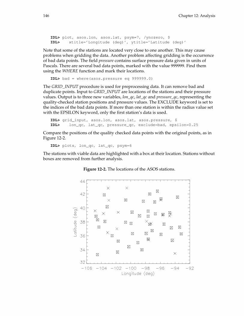
146 Chapter 12: Analysis
IDL> plot, asos.lon, asos.lat, psym=7, /ynozero, $IDL> xtitle=’Longitude (deg)’, ytitle=’Latitude (deg)’
Note that some of the stations are located very close to one another. This may cause problems when gridding the data. Another problem affecting gridding is the occurrence of bad data points. The field pressure contains surface pressure data given in units of Pascals. There are several bad data points, marked with the value 999999. Find them using the WHERE function and mark their locations.
IDL> bad = where(asos.pressure eq 999999.0)
The GRID_INPUT procedure is used for preprocessing data. It can remove bad and duplicate points. Input to GRID_INPUT are locations of the stations and their pressure values. Output is to three new variables, lon_qc, lat_qc and pressure_qc, representing the quality-checked station positions and pressure values. The EXCLUDE keyword is set to the indices of the bad data points. If more than one station is within the radius value set with the EPSILON keyword, only the first station’s data is used.
IDL> grid_input, asos.lon, asos.lat, asos.pressure, $IDL> lon_qc, lat_qc, pressure_qc, exclude=bad, epsilon=0 .25
Compare the positions of the quality checked data points with the original points, as in Figure 12-2.
IDL> plots, lon_qc, lat_qc, psym=6
The stations with viable data are highlighted with a box at their location. Stations without boxes are removed from further analysis.
Figure 12-2. The locations of the ASOS stations.

Chapter 12: Analysis 147
Next, set up a grid. The nodes of a grid with 0.5 degree resolution, with domain [104 W < longitude < 94 W] and [34 N < latitude < 42 N] are defined by the following two vectors.
IDL> lon_vec = findgen(21)/20*10 - 104IDL> lat_vec = findgen(17)/16*8 + 34
Finally, the GRIDDATA procedure can be called to interpolate the irregularly spaced station data to a regular grid. The inputs to GRIDDATA are the quality checked variables output from GRID_INPUT. The default inverse distance method is used for interpolation. A better method could be chosen based on knowledge of the data (pressure is a smooth field variable at this scale in the atmosphere).
IDL> pressure_grid = griddata(lon_qc, lat_qc, pressure_q c, $IDL> /inverse_distance, power=3, /grid, xout=lon_vec, $IDL> yout=lat_vec)
Display the gridded surface pressure data, converting the pressure values from Pa to hPa, a meteorological convention.
IDL> shade_surf, pressure_grid*1e-2, lon_vec, lat_vec, $IDL> charsize=1.5, ax=45, xtitle=’Longitude (deg)’, $IDL> ytitle=’Latitude (deg)’, ztitle=’Pressure (hPa)’
Compare your results with Figure 12-3.
Figure 12-3. The pressure surface from the gridded ASOS data.

148 Chapter 12: Analysis
Curve fitting
Curve fitting is the process of representing a set of observations (e.g., measurements from an instrument) via a model with tunable parameters. The selection of the model is critical; often, it is based on theory underlying the observations. The model parameters are adjusted to minimize a statistic of merit. The value of the statistic of merit can be used to quantify how well the model fits the data. Additional goodness-of-fit tests can also be performed to verify the appropriateness of the model.
Refer to the Online Help for a complete list of curve and surface fitting routines, as well as goodness-of-fit tests, included in IDL.
Two examples of curve fitting are presented in the following sections.
Least-squares linear fit
Linear least squares is probably the most commonly used method of curve fitting. The LINFIT function fits paired data {x i ,y i } to the linear model y = A + Bx by minimizing the chi-square error statistic.
Load the ‘wind’ data set. These data are from a tower-mounted sonic anemometer located at a field site in southeastern Kansas.
IDL> wind = load_data(’wind’)
The variable wind returned by LOAD_DATA is a structure variable with fields time and speed, giving the time stamp (in seconds) and wind speed (in meters per second) of a set of 50 observations.
Use LINFIT to determine the coefficients of the fit. The authors of Numerical Recipes in C assert that a fitting routine should provide the coefficient values, error estimates for the coefficients, as well as a statistical measure of the goodness-of-fit. These are calculated in LINFIT and returned through keyword parameters.
IDL> coefficients = linfit(wind.time, wind.speed, yfit=s peed_fit, $IDL> chisq=chisq, prob=prob, sigma=sigma)
Display the original data and the linear fit. Compare your results with Figure 12-4 below.
IDL> plot, wind.time, wind.speed, ynozero=1, yrange=[2,5 ], psym=1, $IDL> xtitle=’time (s)’, ytitle=’wind speed (ms!u-1!n)IDL> oplot, wind.time, speed_fit
Print the values of the coefficients with their error estimates, as well as the chi-square value for the fit.
IDL> format=’(a15,f5.2,1x,"+/-",f5.2)’IDL> print, ’intercept:’, coefficients[0], sigma[0], for mat=formatintercept: 3.37 +/- 0.11IDL> print, ’slope:’, coefficients[1], sigma[1], format= formatslope: 0.19 +/- 0.04IDL> print, ’chi-square value:’, chisqchi-square value: 7.43271

Chapter 12: Analysis 149
Figure 12-4. An example of linear least-squares regression with LINFIT.
A result similar to that displayed in Figure 12-4 can be achieved with an iTool. Load the wind data into an iTool with the following statement:
IDL> iplot, wind.time, wind.speed, xrange=[0,5], yrange= [2,5], $IDL> linestyle=6, sym_index=1, xtitle=’time (s)’, $IDL> ytitle=’wind speed (ms!u-1!n)’
Within the iTool, execute these two steps:
1. Open the iTools Curve Fitting dialog by selecting Operations > Filter > Curve Fitting from the iTools Menu Bar. By default, a linear fit is calculated. Note that the coefficients and chi-square value match the output from LINFIT.
2. Click “OK” in the Curve Fitting dialog to return to the iTool. The curve fit is now displayed with the data in the iTool.
Least-squares user-defined fit
Often, a nonlinear fit is needed. The SVDFIT function can compute a least-squares fit to an arbitrary user-supplied model, using a singular value decomposition method. The model must be written as an IDL function.
Enter a vector of heights (in meters) and 15-minute mean wind speed values (in meters per second) at those heights.
IDL> heights = [0.1, 3.0, 5.0, 10.0]IDL> wind_profile = [0.00, 5.10, 5.67, 6.67]
The first height is an estimate of the aerodynamic roughness length, the level above the surface at which the wind speed is zero. The remaining heights are the levels at which the

150 Chapter 12: Analysis
instruments—propeller-vane anemometers—are mounted. These data are from the same field site as the sonic anemometer data used in the previous section.
Display a plot of the wind profile, with the independent variable heights on the vertical axis.
IDL> iplot, wind_profile, heights, linestyle=6, sym_inde x=6, $IDL> xtitle=’wind speed (ms!u-1!n)’, ytitle=’height (m)’
The “law of the wall” from fluid mechanics suggests the use of a logarithmic or logsquare model to describe these measurements. If U is wind speed and z is height, the logsquare model can be written
which can be solved for the coefficients a0, a1 and a2. In IDL, this model is represented by the function WIND_PROFILE_MODEL, found in the file of the same name in the introduction directory.
wind_profile_model
function wind_profile_model, x, m
return, [1.0, alog(x), alog(x)^2]end
Note that the return array has three elements, one for each term of the logsquare model. The two parameters, x and m, are required by SVDFIT.
Call SVDFIT to perform the curve fit.
IDL> c = svdfit(heights, wind_profile, $IDL> a=[1.0, 1.0, 1.0], chisq=chisq, sigma=sigma, $IDL> function_name=’wind_profile_model’)
The keyword A is used to input initial guesses for the model coefficients. The FUNCTION_NAME keyword specifies the name of the IDL function representing the model. CHISQ and SIGMA are output keywords, giving the chi-square value of the fit and the standard deviations of the coefficients, respectively. The values of the coefficients are returned in the variable c.
Use the coefficients returned from SVDFIT to make a pair of vectors describing the fit.
IDL> z_fit = findgen(60)/5 + heights[0]IDL> u_fit = c[0] + c[1]*alog(z_fit) + c[2]*alog(z_fit)^ 2
Plot the fit over the original data points.
IDL> iplot, u_fit, z_fit, color=[255,0,0], /overplot
Compare your results with Figure 12-5 below.
U z( ) a0 a1 zln( ) a2 zln( )2
+ +=

Chapter 12: Analysis 151
Figure 12-5. Wind profile data fit with a logsquare model using SVDFIT.
Signal processing
A signal is the record of a process that occurs over an interval of time, space or some arbitrary measure. A signal, by definition, contains information, but any signal obtained from a physical process also contains noise. It is often difficult to make sense of the information contained in a signal by looking at it in its raw form.
Signal processing is the body of methods used to analyze and extract quantitative information from signals. Different disciplines in science and engineering have developed different techniques to extract necessary information from the signals they study.
IDL provides a variety of tools for the processing of one- and multi-dimensional signals. Most are based on the fast Fourier transform (FFT) or the wavelet transform (WT). Refer to the Online Help for a complete list of signal processing routines included in IDL.
Here’s an example of Fourier filtering a time series with an order 5 lowpass Butterworth filter. The data are sea surface temperature anomalies recorded in the equatorial Pacific ocean, describing the El Niño-Southern Oscillation (ENSO). The data are seasonally subsampled with three-month average values from the NINO3 data set over the period 1871-1996.

152 Chapter 12: Analysis
Locate the ENSO data set and read it into IDL.
IDL> file = filepath(’elnino.dat’, subdir=[’examples’,’d ata’])IDL> enso = read_binary(file, data_type=4, endian=’littl e’)
Construct parameters from the data set. A vector of time values is necessary, as well as the interval between the values. This information is not included with the data set. The Nyquist frequency is a property of the data; it quantifies the minimum resolvable frequency, as set by the sampling interval.
IDL> n_enso = n_elements(enso)IDL> delta = 0.25IDL> time = findgen(n_enso)*delta + 1871IDL> freq_nyquist = 0.5/delta
Transform the ENSO data to the frequency domain with the FFT function. The variable enso_hat gives the Fourier coefficients of the data. It is of type complex.
IDL> enso_hat = fft(enso)
Compute the power spectrum of the transformed series by squaring the magnitude of the Fourier coefficients.
IDL> enso_psd = abs(enso_hat)^2
Mark the cutoff frequency for filtering at two-tenths of the Nyquist frequency. This translates to a period of roughly 30 months for these data. The contribution from any Fourier coefficient larger than this value will be attenuated or suppressed entirely, based on the response of the filter.
IDL> freq_c = 0.2*freq_nyquist
Construct an order 5 Butterworth lowpass filter based on the cutoff frequency selected.
IDL> order = 5IDL> kernel = (dist(n_enso))[*,0]/(n_enso*delta)IDL> filter = 1 / (1 + (kernel/freq_c)^(2*order))
Apply the filter to the ENSO time series: multiply it by the transformed series, then apply the inverse FFT to transform the result back to the time domain. The result is a lowpass filtered signal.
IDL> enso_lpf = fft(enso_hat*filter, /inverse)
Display the one-sided power spectrum of the ENSO data plotted versus Fourier mode in a new iTool.
IDL> iplot, enso_psd, identifier=enso_plot, color=[0,100 ,0], $IDL> xrange=[0,n_enso/2], xtitle=’Mode’, ytitle=’PSD’, $IDL> title=’ENSO Temperature Anomaly Record’
Display the filter on the spectrum plot. Note that the filter has unit amplitude, but it is scaled to fit in this plot window. By displaying the filter with the spectrum, you can get a sense of what Fourier modes are filtered out.
IDL> iplot, filter*max(enso_psd), /overplot, color=[255, 220,0], $IDL> xrange=[0,n_enso/2], yrange=[0,max(enso_psd)]
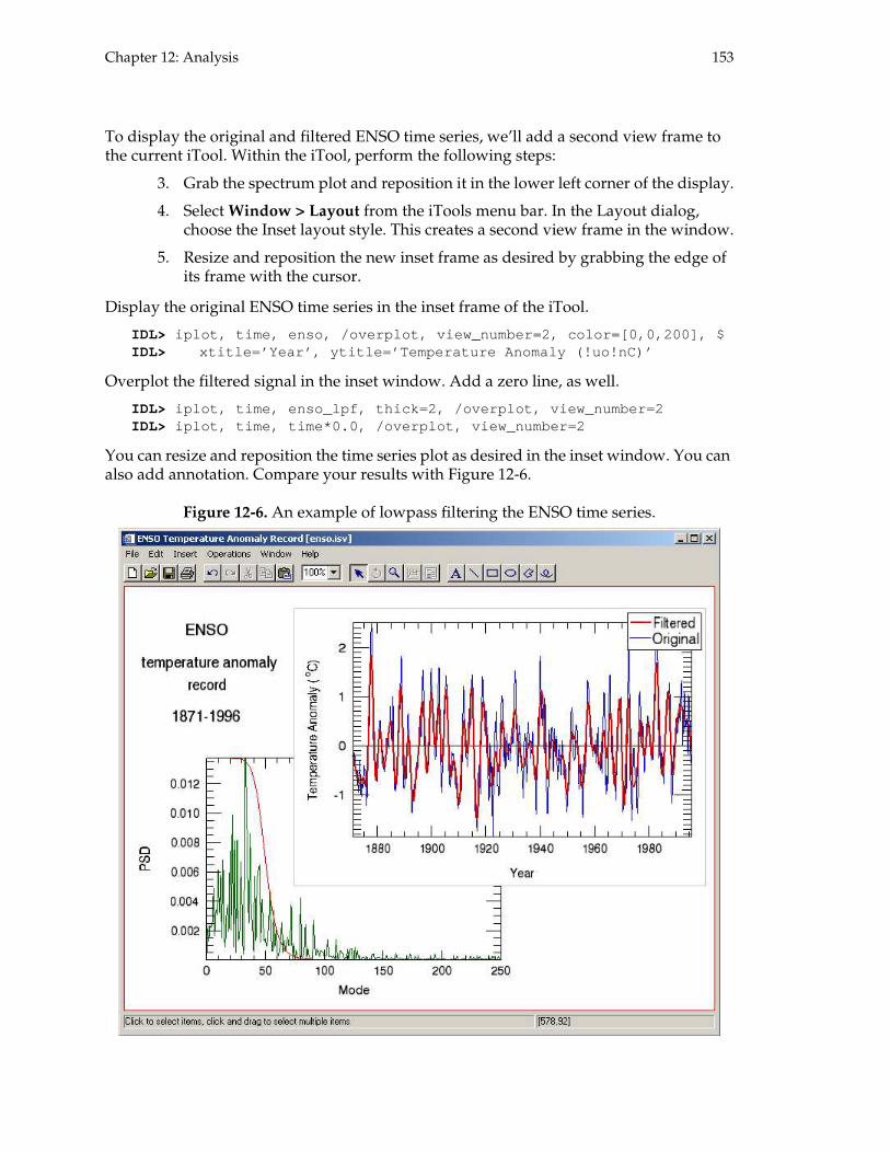
Chapter 12: Analysis 153
To display the original and filtered ENSO time series, we’ll add a second view frame to the current iTool. Within the iTool, perform the following steps:
3. Grab the spectrum plot and reposition it in the lower left corner of the display.
4. Select Window > Layout from the iTools menu bar. In the Layout dialog, choose the Inset layout style. This creates a second view frame in the window.
5. Resize and reposition the new inset frame as desired by grabbing the edge of its frame with the cursor.
Display the original ENSO time series in the inset frame of the iTool.
IDL> iplot, time, enso, /overplot, view_number=2, color= [0,0,200], $IDL> xtitle=’Year’, ytitle=’Temperature Anomaly (!uo!nC) ’
Overplot the filtered signal in the inset window. Add a zero line, as well.
IDL> iplot, time, enso_lpf, thick=2, /overplot, view_num ber=2IDL> iplot, time, time*0.0, /overplot, view_number=2
You can resize and reposition the time series plot as desired in the inset window. You can also add annotation. Compare your results with Figure 12-6.
Figure 12-6. An example of lowpass filtering the ENSO time series.

154 Chapter 12: Analysis
Image processing
Much scientific information, in fields ranging from cellular biology to medicine to astronomy, is communicated through the use of imagery. To extract information from imagery, researchers rely on the body of methods called image processing. Here, we look at examples from a few categories under this heading.
Note there is a new manual, Image Processing in IDL, in the IDL documentation set. It can be accessed through the Contents tab of the IDL Online Help browser under the heading User’s Guides. It can also be purchased in hardcopy format from RSI. There are many more examples there in its 500+ pages than can be presented in the confines of this course manual.
Median filtering
Median smoothing replaces each pixel in an image with the median (the value in an ordered set with an equal number of values above and below it) of the two-dimensional neighborhood of a given width. It is similar to smoothing with a boxcar or average filter but does not blur edges larger than the neighborhood. Median filtering is effective in removing "salt and pepper" noise, (isolated high or low values).
Load an image with the course program LOAD_DATA.
IDL> ali = load_data(’people’)IDL> asize = size(ali, /dimensions)
Make a new image speckled with approximately 1000 (or 1e3: IDL allows scientific notation) white and black pixels at random locations. Note the use of the single-index subscripting method.
IDL> noisy = aliIDL> white_points = randomu(seed, 1e3)*asize[0]*asize[1]IDL> noisy[white_points] = 255BIDL> black_points = randomu(seed, 1e3)*asize[0]*asize[1]IDL> noisy[black_points] = 0B
Using TV, display the original, noisy and filtered images in a new Direct Graphics window.
IDL> window, xsize=asize[0]*3, ysize=asize[1], $IDL> title=’Median Filtering Example’IDL> tv, ali, 0IDL> tv, noisy, 1IDL> tv, median(noisy, 3), 2
Compare your results with Figure 12-7 on page 155.

Chapter 12: Analysis 155
Figure 12-7. An example of median filtering a noisy image.
Histogram equalization
In histogram equalization, image pixel values are rearranged to spread the image’s histogram over the byte range. This typically enhances the contrast between neighboring regions. Some pixels with values that are different initially may be assigned the same value. Other pixel values may be missing entirely. Histogram equalization is an example of global contrast enhancement.
Start by reading an image from a file. This image represents a model of convection in the Earth’s mantle.
IDL> file = filepath(’convec.dat’, subdir=[’examples’,’d ata’])IDL> isize = [248,248]IDL> mantle = read_binary(file, data_dims=isize)
Set up an iTool and display the image in it. By setting the VIEW_GRID keyword to IIMAGE, the resulting iTool will have four view areas, arranged in a 2 x 2 grid. The IDENTIFIER keyword is set to a variable that can be used to identify this particular iTool at a later stage.
IDL> iimage, mantle, dimensions=isize*2, view_grid=[2,2] , $IDL> title=’Histogram Equalization Example’, xtickfont_s ize=6, $ IDL> ytickfont_size=6, identifier=this_tool
Use the HISTOGRAM function to calculate the image's histogram, or frequency distribution; this is the graph of the number of times a given pixel value occurs in the image, as a function of that pixel value. With IPLOT, display the histogram in the second view position in the iTool, using the OVERPLOT and VIEW_NUMBER keywords. Any value greater than that set with the MAX_VALUE keyword is not plotted.
IDL> iplot, histogram(mantle), overplot=this_tool, view_ number=2, $IDL> xtickfont_size=6, ytickfont_size=6, max_value=5000, $IDL> xtitle=’pixel value’, ytitle=’# of occurences’

156 Chapter 12: Analysis
Apply the HIST_EQUAL function to the image. Display the results in the third view position in the iTool.
IDL> eq_mantle = hist_equal(mantle)IDL> iimage, eq_mantle, overplot=this_tool, view_number= 3, $IDL> xtickfont_size=6, ytickfont_size=6
Finally, calculate and display the equalized image’s histogram in the fourth view position in the iTool.
IDL> iplot, histogram(eq_mantle), overplot=this_tool, $IDL> view_number=4, xtickfont_size=6, ytickfont_size=6, $IDL> max_value=5000, xtitle=’pixel value’, $IDL> ytitle=’# of occurences’
Compare your results with Figure 12-8.
Figure 12-8. An example of image contrast enhancement with histogram equalization.

Chapter 12: Analysis 157
Image sharpening
Image sharpening is an example of local contrast enhancement. The Laplacian operator sharpens the image by locally increasing the contrast at discontinuities and improving image contrast at edges. Sharpening an image also increases the contrast between light and dark areas to enhance features in an image.
Image sharpening techniques are plentiful. Here is one method adapted from the authors listed in the “Suggested reading” section at the end of this chapter.
Read an image from a file. The image is a photomicrograph of endothelial cells in a cow.
IDL> file = filepath(’endocell.jpg’, subdir=[’examples’, ’data’])IDL> read_jpeg, file, cells
Load the grayscale color table. Make a window the same size as the image and display the image in it.
IDL> loadct, 0, /silentIDL> info = size(cells, /structure)IDL> window, 0, xsize=info.dimensions[0], ysize=info.dim ensions[1], $IDL> title=’Original Image’IDL> tvscl, cells
Make a 3 x 3 Laplacian kernel.
IDL> kernel = intarr(3,3) - lIDL> kernel[1,1] = 8IDL> print, kernel
-1 -1 -1-1 8 -1-1 -1 -1
Cast the image data to type signed short integer with the FIX function. The highpass filtered image that results from convolution with the Laplacian operator has both positive and negative values. If the image remained type byte, the negative values would simply be wrapped into the byte range.
IDL> cells = fix(cells)
Apply the 3 x 3 Laplacian operator with the CONVOL function.
IDL> hipass = convol(cells, kernel, /center)
Bytescale the highpass filtered image (remember it has positive and negative values) and display it.
IDL> hipass = bytscl(hipass)IDL> window, 1, xsize=info.dimensions[0], ysize=info.dim ensions[1], $IDL> title=’Highpass Filtered Image’IDL> tv, hipass
The Laplacian operator enhances portions of an image where substantial change occurs, such as lines and edges. It suppresses uniform and slowly varying regions. In this image, note that the edges of the cell walls and the nucleus have brighter intensities.

158 Chapter 12: Analysis
To complete the sharpening process, add the highpass filtered image to the original. Bytescale the result and display.
IDL> new = cells + hipassIDL> window, 2, xsize=info.dimensions[0], ysize=info.dim ensions[1], $IDL> title=’Sharpened Image’IDL> tv, bytscl(new)
Figure 12-9 shows the result of applying this sharpening technique to the image in the file endocell.jpg, with a side-by-side view.
Figure 12-9. Portions cropped from the original (left) and sharpened image (right).
Edge enhancement
Detection of edges in images can be useful. The Laplacian operator can emphasize regions of sharp change in images, but because of its symmetry it is insensitive to direction. More specialized operators can be used to emphasize the direction of edges, such as the Sobel operator and the Roberts cross-gradient operator. These operators work by only estimating derivatives in certain directions. IDL has several built-in edge-enhancing routines.

Chapter 12: Analysis 159
Display the image in the variable ali, from the section “Median filtering” on page 154, as well as versions of the image filtered with the SOBEL and ROBERTS functions.
IDL> window, xsize=asize[0]*3, ysize=asize[1], $IDL> title=’Edge Detection Example’IDL> tv, ali, 0IDL> tv, sobel(ali), 1IDL> tv, roberts(ali), 2
Compare your results with Figure 12-10.
Figure 12-10. An image filtered with the SOBEL and ROBERTS edge-enhancing routines.
Exercises
1. Try constructing a polynomial interpolant to the data presented in Figure 12-1 on page 145 using the POLY_FIT function.
2. With LOAD_DATA, load the data set ’world_elevation’ into your IDL session. Display it as an image. Can you create an image mask so that only the elevations above sea level are displayed? Hint: Sea level is approximately 124.
3. Parseval’s theorem test: does the integral of the spectrum equal the variance of the ENSO series in the example in the “Signal processing” section?
4. Unsharp masking is the process of removing low-frequency information from an image, leaving only high-frequency details. Can you construct an unsharp masked image from the data in the variable ali, used above? Hint: Use the SMOOTH function.
5. Try constructing the negative of an indexed image. Can you also construct the negative of a 24-bit True Color image?

160 Chapter 12: Analysis
Suggested reading
Press, W.H., B.P. Flannery, S.A. Teukolsky and W.T. Vetterling. Numerical Recipes in C: The Art of Scientific Computing. Cambridge, England: Cambridge University Press. 1988.
A handbook of scientific computing in C. Many analysis routines in IDL are derived from the programs in this text.
Bendat, J.S. and A.G. Piersol. Random Data; Analysis and Measurement Procedures. New York, New York: Wiley, 1971.
Priestley, M.B. Spectral Analysis and Time Series. San Diego, California: Academic Press, 1981.
These texts deal with signal processing techniques. Priestley’s book is very dense.
Gonzales, R.C. and R.E. Woods. Digital Image Processing. Reading, Massachusetts: Addison-Wesley, 1992.
Russ, J.C. The Image Processing Handbook. Second edition. Boca Raton, Florida: CRC Press, 1995.
These texts deal with image processing techniques.
Kling, R.L. Application Development with IDL: Combining analytical methods with widget programming. Warrenton, Virginia: Ronn Kling Consulting, 1999.
This useful text implements several analysis techniques in IDL, including active contours, simulated annealing and watershed segmentation.
Research Systems. Image Processing in IDL. Boulder, CO: Research Systems, 2005.
This new RSI manual discusses many common image processing techniques and gives examples of how they can be implemented in IDL. Access it from the Contents tab of the Online Help, under User’s Guides.

161
Chapter 13:
Map Projections
This chapter describes how to create map projections and display data on them.
Map projections . . . . . . . . . . . . . . . . . . . . . . . 162Creating a map projection . . . . . . . . . . . . . . . 162Displaying data on a map projection . . . . . 163 Displaying data with contours . . . . . . . . . . 164 Displaying data with an image . . . . . . . . . 166
Converting data between map projections 167The iMap iTool . . . . . . . . . . . . . . . . . . . . . . . 169Exercises . . . . . . . . . . . . . . . . . . . . . . . . . . . . . 170Suggested reading . . . . . . . . . . . . . . . . . . . . 171

162 Chapter 13: Map Projections
Map projections
A map projection is a transformation relating coordinates on a curved surface to coordinates on a plane. Historically, the idea of a map projection arose from the need to represent locations on the (approximately) spherical surface of the Earth on a piece of paper.
The problem with map projections is that sizes, shapes and distances can be distorted in the transformation from curved to planar coordinates. To address this problem, a variety of map projections have been developed, each employing different techniques to deform a spherical surface into a planar surface by stretching or cutting the surface, thus minimizing distortion in particular locations.
Map projections are particularly useful for displaying certain scientific data sets with a wide geographical extent; for example, in geophysics, map projections are used to display global sea surface temperatures, polar sea ice distributions and surface weather maps.
IDL has the ability to generate map projections, convert data between projections and display data on them. IDL has 19 built-in map projections, as well as an interface to many more available from the U.S. Geological Survey General Cartographic Transformation Package (GCTP). For examples of what the different projections look like, see Chapter 9, “Map Projections” in Using IDL, or visit the USGS Map Projections website at http://mac.usgs.gov/mac/isb/pubs/MapProjections/pro jections.html
Examples of how to construct map projections and display data on them follow.
Creating a map projection
IDL has two primary routines for creating map projections: MAP_SET and MAP_PROJ_INIT. The MAP_SET procedure is used to define a map projection inside a Direct Graphics window. Data in latitude/longitude coordinates can then be displayed in this window. The MAP_PROJ_INIT function is more general; it returns a map projection that can be used with the MAP_PROJ_FORWARD or MAP_PROJ_INVERSE functions to convert latitude/longitude coordinates into Cartesian coordinates (or vice-versa) for use in a Direct or Object Graphics visualization.
Here is a quick example of using MAP_SET, along with some helper routines, to draw a simple map in Direct Graphics.
Start by loading a color table and creating a Direct Graphics window.
IDL> loadct, 39IDL> window, 0, xs=400, ys=500, title=’Map Example’
Use MAP_SET to create a Mercator map projection inside the current graphics window. Several keywords are used here to alter the default behavior of MAP_SET. A description of each follows. The ISOTROPIC keyword is set to force equal increments in latitude and longitude in the projection. If this keyword is not set, the projection fills the graphics window. The E_HORIZON keyword modifies the background of the projection in the

Chapter 13: Map Projections 163
display window. Here it is set to a structure variable asserting that the background should be filled with color 50 from the current color table. The LIMIT keyword is set to four-element array describing the geographical bounds of the projection. In this case, the map projection is limited to a box bounded by 60o S latitude, 90o W longitude, 20o N latitude and 30o W longitude. The YMARGIN keyword is set to 3 characters from the edge of the window.
IDL> map_set, /mercator, /isotropic, e_horizon={fill:1, color:50}, $IDL> limit=[-60,-90,20,-30], ymargin=3
Note that after executing this statement, no information (other than the blue background) appears inside the window. This is because we have only set up the coordinate system, nothing has been displayed in it.
Draw a grid of parallels and meridians with the MAP_GRID procedure.
IDL> map_grid, /box_axes, color=255, charsize=0.8
Draw coastal outlines with the MAP_CONTINENTS procedure.
IDL> map_continents, /coasts, color=0, thick=3
MAP_CONTINENTS may employ either a low-resolution (20 km) or a high-resolution (1 km) mapping database. The low-resolution database is the default. The high-resolution database may be installed optionally with IDL. If it is present, it can be accessed with the HIRES keyword. Both databases are adapted from the 1993 CIA World Map database by Thomas Oetli of the Swiss Meteorological Institute.
Use MAP_CONTINENTS again to draw the continents and fill them with color 160 from the color table.
IDL> map_continents, color=160, fill_continents=1
Note that successive applications of MAP_CONTINENTS act like layers on the visualization. Finally, draw political boundaries.
IDL> map_continents, /countries, color=0
With the execution of this last step, you should have a map of South America that looks like Figure 13-1 on page 164.
Displaying data on a map projection
The map in Figure 13-1 may be pretty, but the point of having map projections available in IDL is for displaying data on them.
Examples of displaying data on map projections with contours and as an image follow.

164 Chapter 13: Map Projections
Figure 13-1. A map generated with IDL mapping routines.
Displaying data with contours
In the section “Gridding irregularly spaced data” on page 145, we used the IDL routine GRIDDATA to interpolate Automated Surface Observing System (ASOS) surface weather data to a regular grid. Gridded surface temperature data from this exercise are stored in an IDL save file, gridded_temperature.sav, in the introduction directory. Restore the contents of this file to your IDL session.
IDL> file = filepath(’gridded_temperature.sav’, $IDL> root_dir=get_intro_dir())IDL> restore, file
This save file contains five IDL variables: g_temp, g_lon, g_lat, lon and lat, corresponding to the gridded temperature data, the latitude and longitude grid for these data, and the original locations of the ASOS stations. The grid is 21 x 17, with 0.5 degree resolution, starting at the location 104o W longitude, 34o N latitude, increasing north and east.
Use MAP_SET to create a map projection in a Direct Graphics window. Here, the NAME keyword is used as an alternate means of specifying the map projection; in this case, a Mollweide projection. Using the LIMIT keyword, the projection is limited to the

Chapter 13: Map Projections 165
geographic area bounded by 33o N latitude, 106o W longitude, 43o N latitude and 92o W longitude.
IDL> window, 1, title=’Map-Contour Example’IDL> map_set, name=’Mollweide’, /noborder, /isotropic, $IDL> limit=[33.0, -106.0, 43.0, -92.0]
Use the USA keyword to MAP_CONTINENTS to draw U.S. state boundaries on the projection. Also, display the locations of the ASOS stations with triangles using PLOTS.
IDL> map_continents, /usaIDL> plots, lon, lat, psym=5
Now, display the data on the map projection with a contour plot. Note that the longitude and latitude vectors for the grid, g_lon and g_lat, must be passed to CONTOUR in addition to the gridded temperature data. Also note the OVERPLOT keyword must be set, so that CONTOUR doesn’t erase the graphics already present in the window.
IDL> loadct, 5IDL> contour, g_temp, g_lon, g_lat, /overplot, /follow, $ IDL> levels=indgen(11)*2 + 278, c_colors=indgen(11)*20 + 20
Compare your results with Figure 13-2. A professional meteorologist would probably adjust the plot slightly, packing the isotherms more closely around the front stretching from southwest to northeast across Kansas.
Figure 13-2. Surface temperature data displayed with contours on a map of the U.S. Great Plains.
166 Chapter 13: Map Projections
Displaying data with an image
Data in the form of an image are fundamentally expressed in a Cartesian coordinate system. To display the data on a map projection, the image needs to be transformed to the projection coordinate system. Depending on the location and the type of projection, extreme warping may occur. IDL has two built-in routines for transforming image data to map coordinates, MAP_IMAGE and MAP_PATCH.
In this example, we use the gridded ASOS surface temperature data from the previous section, although instead of using contours, we display the data as an image.
Start by creating a map projection in a new window. Use a Mollweide projection with the same geographic limits as in the previous example.
IDL> window, 2, title=’Map-Image Example’IDL> load_graysIDL> map_set, /mollweide, /noborder, /isotropic, $IDL> limit=[33.0, -106.0, 43.0, -92.0]
Load a color table. Find the geographic extent of gridded data values with the MIN and MAX functions.
IDL> loadct, 5IDL> min_lat = min(g_lat, max=max_lat)IDL> min_lon = min(g_lon, max=max_lon)
Display the data as an image warped to the map projection with MAP_IMAGE. The parameters startx and starty are used to return the start position where TV or TVSCL can draw the image. The COMPRESS keyword controls the accuracy of the transformation to map coordinates. With the BILINEAR keyword set, bilinear interpolation is used instead of nearest neighbor sampling when warping the image. The MISSING keyword is used to set the value of the warped image pixels outside the bounds set by the LATMIN, LONMIN, LATMAX and LONMAX keywords.
IDL> warped_image = map_image(g_temp, startx, starty, co mpress=1, $IDL> latmin=min_lat, latmax=max_lat, lonmin=min_lon, $IDL> lonmax=max_lon, /bilinear, missing=max(g_temp))IDL> tvscl, warped_image, startx, starty
Last, draw the state boundaries over the image.
IDL> map_continents, /usa, color=0
Compare your results with Figure 13-3 below and Figure 13-2, as well.

Chapter 13: Map Projections 167
Figure 13-3. Surface temperature data displayed as an image on a map of the U.S. Great Plains.
Converting data between map projections
For general cartographic conversions, IDL has the routines MAP_PROJ_INIT, MAP_PROJ_FORWARD and MAP_PROJ_INVERSE. These routines can be used to convert data between Cartesian and map projections, or even between different map projections. A simple example of using these routines to display the nodes of a map grid in an iTool is shown here.
Define a map projection with MAP_PROJ_INIT. Use the Mollweide projection to facilitate comparison with the other two examples in this chapter. Likewise, use the same geographic limits. Assume the default datum. The output is a !map-style structure variable (!map itself is not altered).
IDL> map = map_proj_init(’Mollweide’, $IDL> limit=[33.0, -106.0, 43.0, -92.0])
Define the number of grid nodes in latitude and longitude.
IDL> n_lat = 11IDL> n_lon = 15
Set the values of latitude and longitude at these nodes. These vectors define a grid with one degree resolution.
IDL> lon = (findgen(n_lat*n_lon) mod n_lon) - 106.0IDL> lat = (findgen(n_lat*n_lon) mod n_lat) + 33.0

168 Chapter 13: Map Projections
Convert the latitude/longitude grid to Cartesian x/y coordinates with the MAP_PROJ_FORWARD function. Note that the input to MAP_PROJ_FORWARD requires either vectors of latitude and longitude or a 2 x N element array of latitude and longitude values, where N is the number of points.
IDL> grid = map_proj_forward(lon, lat, map_structure=map )
Reform the data for input to an iPlot. Also, scale the data to kilometers instead of meters.
IDL> x = reform(grid[0,*])*1e-3IDL> y = reform(grid[1,*])*1e-3
Display the grid in map coordinates.
IDL> iplot, lon, lat, sym_index=5, linestyle=6, view_gri d=[2,1], $IDL> color=[255,0,0], xtitle=’Longitude (deg W)’, $IDL> ytitle=’Latitude (deg N)’
Display the grid in Cartesian coordinates.
IDL> iplot, x, y, sym_index=5, linestyle=6, /view_next, $IDL> color=[0,0,255], xtitle=’X (km W)’, ytitle=’Y (km N )’
Compare your results to Figure 13-4. Some annotation has been added to the two plots.
Figure 13-4. A latitude-longitude grid displayed in map and Cartesian coordinates.

Chapter 13: Map Projections 169
The iMap iTool
The IMAP procedure creates an iTool that is configured to manipulate georeferenced data and display them as an image or a set of contours. IMAP can also be used to import and display data from a ESRI Shapefile.
Use IMAP to display the georeferenced gridded temperature data with a Mollweide map projection.
IDL> loadct, 5IDL> tvlct, r, g, b, /getIDL> imap, g_temp, g_lon, g_lat, map_projection=’Mollwei de’, $IDL> limit=[33,-105,43,-93], rgb_table=[[r],[g],[b]], $IDL> /contour, n_levels=20, /fill, grid_units=2
Data are displayed in IMAP as an image, unless the CONTOUR keyword is set. The GRID_UNITS keyword is very important in this example, since it is used to state that the vectors g_lon and g_lat are in units of degrees latitude/longitude.
Modify this iTool with the following steps.
1. Launch the Visualization Browser (Window > Visualization Browser...) and select the Map Grid object .
2. Open the right panel of the Visualization Browser and in it, change the Latitude spacing and Longitude spacing properties of the Map Grid to 4 degrees each.
3. Also in the Map Grid properties window, change the Line style property to dotted and the Label position property to 0.
Like MAP_CONTINENTS, IMAP provides the ability to overlay continental outlines, rivers, as well as U.S. state and Canadian provincial boundaries.
4. Insert the boundaries of the Great Plains states by selecting Insert > Map > United States from the Menu Bar.
The image and/or contour objects displayed in the iMap Display can also be manipulated.
5. Select the Contour object in the left panel of the Visualization Browser. Change its Transparency property to a nonzero value (try 30).
Annotation can also be added.
6. Select the contour plot in the Display, then select Insert > Colorbar from the iMap Menu Bar. Move the colorbar to where you’d like it to appear in the Display.
7. In the Visualization Browser, select the Colorbar object . Change its Title property to Temperature (K) and set its Font size property to the same as the Map Grid.
8. Select the Text button on the Tool Bar and give the visualization an appropriate title.
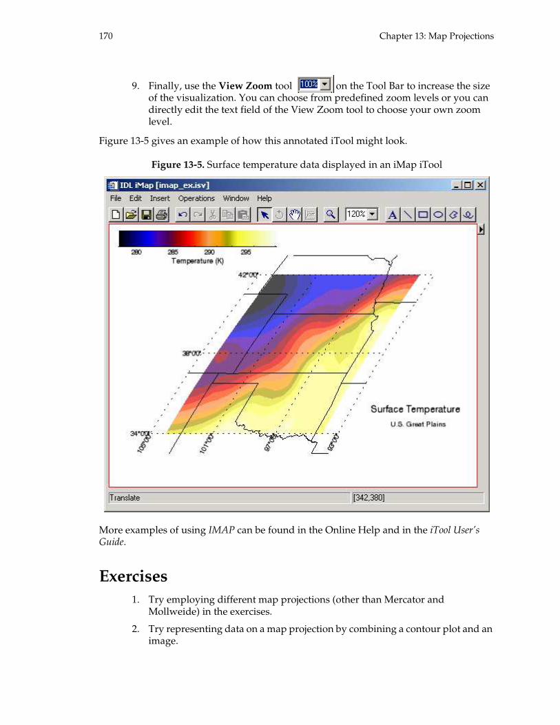
170 Chapter 13: Map Projections
9. Finally, use the View Zoom tool on the Tool Bar to increase the size of the visualization. You can choose from predefined zoom levels or you can directly edit the text field of the View Zoom tool to choose your own zoom level.
Figure 13-5 gives an example of how this annotated iTool might look.
Figure 13-5. Surface temperature data displayed in an iMap iTool
More examples of using IMAP can be found in the Online Help and in the iTool User’s Guide.
Exercises
1. Try employing different map projections (other than Mercator and Mollweide) in the exercises.
2. Try representing data on a map projection by combining a contour plot and an image.
Chapter 13: Map Projections 171
3. Can you represent a straight line on the Earth’s surface on a map projection? Hint: a straight line on the Earth’s surface is a great circle.
Suggested reading
Research Systems. Using IDL. Boulder, Colorado: Research Systems, 2005.
Chapter 9 of this manual describes and gives examples of the use of the map projection routines in IDL.
Snyder, J.P. Map Projections—A Working Manual. U.S.Geological Survey Professional Paper 1395. Washington, D.C.: U.S. Government Printing Office, 1987.
This USGS publication is one of the standards in working with map projections. Other USGS map projection publications are listed at http://mac.usgs.gov/mac/isb/pubs/factsheets/fs08799 .html

172 Chapter 13: Map Projections
173
Chapter 14:
Strings
Strings have a wide variety of common uses, including managing file names, parsing data files, and handling user input in widget programs.
In IDL, strings are primitive data types, so there are built-in string operators such as + for concatenation as well as a powerful library of string functions, including regular expressions.
Special characters and string operators . . . 174Summary of string routines . . . . . . . . . . . . . 174String functions . . . . . . . . . . . . . . . . . . . . . . . 175 Basic string functions . . . . . . . . . . . . . . . . . . 175
Substrings and comparisons . . . . . . . . . . . 176Regular expression searching and splitting 178Exercises . . . . . . . . . . . . . . . . . . . . . . . . . . . . . 181Suggested reading . . . . . . . . . . . . . . . . . . . . 182

174 Chapter 14: Strings
Special characters and string operators
’ and " characters
Literal strings are created with either single or double quotes; though single quotes are highly recommended (see Exercise 3 on page 182). Single or double quotes can be nested one level deep; for example,
IDL> print, ’See "Spot" run’See "Spot" run
+
The + operator concatenates strings. The + operator for strings works in the same way for arrays as the standard numeric + operator; one or both operands may be a string array. For example,
IDL> print, ’a’ + [’b’, ’c’]ab ac
If one of the operands is a string representation of a numeric type, the result will be numeric:
IDL> print, 4 + ’5’<Expression> INT = 9
EQ NE
The EQ and NE operators determine if two strings or two string arrays are exactly equal (case-sensitive). Use STRCMP for case-insensitive comparison.
LT LE GT GE
The LT, LE, GT, and GE operators compare strings or string arrays in lexigraphic order. For example,
IDL> print, ’Hello’ lt ’hello’1
This result is based on the ASCII code for uppercase versus lowercase ’h’:
IDL> print, byte(’H’), byte(’h’)72 104
Note that the < and > operators do not work with strings.
Summary of string routines
IDL contains a library of powerful routines for string processing. The routines in the library enable string conversion, searching, splitting, joining, comparison and regular expression pattern matching. The 14 functions in the IDL string library are listed in Table 14-1 and discussed below. The first argument for each of the function should be a string (or, possibly, a string array), but is converted automatically to a string using the

Chapter 14: Strings 175
default formatting rules if it is not. The default formatting rules will usually result in leading blank spaces.
String functions
Basic string functions
The first set of string manipulation functions in IDL perform basic string manipulation functions such as finding the length of a string, converting to upper or lower case and removing white space from a string.
STRING
Use the STRING function to convert a numeric type to a string.
IDL> print, string(123L)123
The default formatting rules are used (the same as the PRINT procedure’s), but may be changed using C or Fortran format codes in the FORMAT keyword.
An important special case, is that the STRING function will convert a byte array to a scalar string using the ASCII table. Similarly, the BYTE function will convert a scalar string to a byte array. For example,
IDL> print, byte(’IDL’)73 68 76
where the ASCII codes for the letters I-D-L are 73, 68, and 76 respectively.
Table 14-1. IDL string manipulation functions.
Function Purpose
STRCMP Compares two strings
STRCOMPRESS Removes white space from a string
STREGEX Performs regular expression pattern matching
STRING General string conversion function
STRJOIN Collapses a string array into merged scalar string
STRLEN Returns the length of a string
STRLOWCASE Converts a string to lower case
STRMATCH Compares a search string against an input string expression
STRMID Extracts a substring from a string
STRPOS Finds the first occurrence of a substring in a string
STRPUT Inserts the contents of one string into another
STRSPLIT Splits its input string into an array of separate substrings
STRTRIM Converts to string (if necessary) and removes leading and/or trailing blanks
STRUPCASE Converts a string to upper case

176 Chapter 14: Strings
STRLEN
To find the length of a string, use the STRLEN function.
IDL> str = ’It is a beautiful day in the neigh borhood’IDL> print, strlen(str)
51
STRUPCASE/STRLOWCASE
Strings can be converted to upper or lower case with STRUPCASE or STRLOWCASE.
IDL> ustr = strupcase(str)IDL> print, ustrIT IS A BEAUTIFUL DAY IN THE NEIGHBORHOODIDL> lstr = strlowcase(str)IDL> print, lstrit is a beautiful day in the neighborhood
STRCOMPRESS
To compress white space in a string down to a single space, use STRCOMPRESS. When the REMOVE_ALL keyword is used, all white space is removed from the string.
IDL> nstr = strcompress(str)IDL> print, nstrIt is a beautiful day in the neighborhoodIDL> rstr = strcompress(str, /remove_all)IDL> print, rstrItisabeautifuldayintheneighborhood
The first call to STRCOMPRESS removes all but one space between words. The second call leaves a string with no white space.
Function calls to string routines can easily be combined to perform several tasks in one line of code.
IDL> print, strlen(strcompress(str, /remove_all))34
IDL> print, strupcase(strcompress(str))IT IS A BEAUTIFUL DAY IN THE NEIGHBORHOOD
Substrings and comparisons
To get more information from a string, the STRCMP, STRMID, STRMATCH, and STRPOS functions along with the STRPUT procedure can be used. These functions compare strings, search strings, find substrings, and replace parts of strings.
STRCMP
The STRCMP function compares two strings for equality. This function is similar to a Boolean comparison using the EQ operator in a logical statement. STRCMP adds functionality such as case-insensitivity and the ability to limit the length of the comparison.
IDL> name1 = ’Jon’

Chapter 14: Strings 177
IDL> name2 = ’jonathan’IDL> print, strcmp(name1, name2) ; Jon eq jonathan
0IDL> print, strcmp(name1, name2, 3) ; Jon eq jon
0IDL> print, strcmp(name1, name2, 3, /fold_case) ; jon eq jon
1
The first call to STRCMP performs a character-by-character comparison of the two strings. The second call uses the optional third argument to specify the length of the comparison. The last call performs a case-insensitive search on the first three characters of each string.
STRMATCH
String comparison with wildcards can be performed using the STRMATCH function. Input scalar strings or string arrays can be searched with wildcards. If a match occurs, STRMATCH returns a 1 for a match or a 0 for no match. Acceptable wildcards are the * and ? wildcards.
IDL> files = [’day10_01’,’day21_01’,’day10_13’, $IDL> ’day15_09’, ’DAY12_45’, ’Day10_45’]IDL> ; find all the files from day 10IDL> fmatch = strmatch(files, ’day10*’, /fold_case)IDL> day10files = files[where(fmatch eq 1)]IDL> print, day10filesday10_01 day10_13 Day10_45IDL> ; find all the files from days 10-19IDL> print, strmatch(files, ’day1?*’, /fold_case)
1 0 1 1 1 1
STRMID
The powerful STRMID function extracts substrings from a string given a beginning position and offset. The following example uses STRMID to extract two characters starting at position 3 from each element in the input string array. Positions in a string start at 0. Position 3 is the fourth character in the string.
IDL> days = strmid(files, 3, 2)IDL> print, fix(days)
10 21 10 15 12 10
STRPOS
The STRPOS function searches a string for the first occurrence of a supplied search string and returns the position in the string of the first match. Searching can occur from the beginning or end of the string and positions can be reported as offsets from the beginning or end of the string. The following example uses STRPOS combined with STRMID to extract the three letter extension from a file name.
IDL> filename = filepath(’rose.jpg’, subdir=[’examples’, ’data’])IDL> dotpos = strpos(filename, ’.’, /reverse_search) ; f ind last dotIDL> print, dotpos
31

178 Chapter 14: Strings
IDL> exten = strmid(filename, dotpos+1, 3) ; find the fi le extensionIDL> print, extenjpg
STRPUT
The STRPUT procedure places a substring into an existing string—overwriting the existing characters in the string. The substring can be placed at any position in the string. For example, to replace the file extension, a simple call to STRPUT is made.
IDL> strput, filename, ’png’, dotpos+1 ; replace the jpg ext with pngIDL> print, filenameC:\RSI\IDL63\examples\data\rose.png
STRPUT does not change the length of its argument.
STRJOIN
The STRJOIN function collapses a scalar string or string array into a single string. When the joining occurs, STRJOIN can also place a delimiter between the joined strings.
IDL> s1 = [’’,’home’,’john’,’idl’]IDL> print, strjoin(s1)homejohnidlIDL> print, strjoin(s1, ’/’)/home/john/idl
The STRJOIN function can be used in conjunction with the STRSPLIT function described in the next section to easily change the delimiters in a string.
Regular expression searching and splitting
IDL fully supports string searching using any Portable Operating System Interface (POSIX) standard regular expression. A regular expression is a pattern that describes a string or set of strings. Regular expressions are constructed in a similar manner to arithmetic expressions using various operators to combine smaller expressions.
STREGEX
To perform regular expression searching use the STREGEX function. After searching and matching occur on the string, the results report in one of three different ways: the position in the string where the match occurred, a true or false (1 or 0) value or the substring that met the criteria. All regular expression searching can be done without regard to case by setting the FOLD_CASE keyword.
The easiest form of regular expression search that is performed is a literal search. In this case, a substring is passed and a match is attempted.
IDL> str = ’Classes: Introduction to IDL / Intermediate IDL’IDL> print, stregex(str, ’Intro’) ; offset returned
9IDL> print, stregex(str, ’idl’, /fold_case, /boolean) ; case insens
1IDL> print, stregex(str, ’Int’, /extract) ; return the m atch string

Chapter 14: Strings 179
Int
More powerful pattern matching can be achieved using one or more of the special characters or definitions accepted by regular expressions. These characters are used to build patterns that can satisfy almost any match requirement. A list of these special characters and definitions is listed Table 14-2.
The first set of characters in that table are repetition characters. These characters search for zero or more matches of the preceding character or expression. Examples of these characters are below.
IDL> str1 = ’abbcccdddeeee’IDL> print, stregex(str1, ’a?’, /extract)aIDL> print, stregex(str1, ’a?f*’, /extract)aIDL> print, stregex(str1, ’c+’, /extract)ccc
Table 14-2. Special characters and definitions in regular expressions.
Character Description Example
. The period matches any character .
? The preceding item is optional and matched at most once.
a?
* The preceding item will be matched zero or more times. ab*c
+ The preceding item will be matched one or more times n+ame
{n} The preceding item is matched exactly n times a{2}
{n, } The preceding item is matched n or more times b{3,}
{,m} The preceding item is optional and matched at most m times
c{,4}
{n,m} The preceding item is matched at least n times, but not more than m times.
d{2, 4}
[] Bracketed expression used to specify one or more characters or a range of characters
[abzdf] [a-z][0-9]
\ Suppress the meaning of the character it precedes, and turn it into an ordinary character
a\+b
( ) A subexpression a(b+)+
| Alternation. One of several possibilities will match a|b|c
[:alnum:] Match any alphanumeric character b[[:alnum:]]
[:alpha:] Match any alphabetic character [[:alpha:]]9
[:digit:] Match any numeric digit day[[:digit:]]
^ The pattern that follows must match at the beginning of the string
^[[:alpha:]]
$ The pattern that precedes must be contained at the end of the string
[[:digit:]]$

180 Chapter 14: Strings
The first STREGEX statement matches one instance of the character a in the string. The second matches one instance of a followed by zero or more instances of f and the third matches one or more instances of c.
IDL> print, stregex(str1, ’(e{2})+’, /extract, /subexpr)eeee eeIDL> print, stregex(str1, ’e{2,3}’)
9
The first statement above uses a subexpression, contained within parentheses. To have subexpressions evaluated, the SUBEXPR keyword must be set.
The last set of characters in Table 14-2 are special definitions that can be used to match well defined ranges of characters, such as numbers and digits. Square brackets can be used to match one of a set of characters or one of a range of characters. The square brackets can also contain one of many special definitions contained in regular expressions. Consider the following examples.
IDL> s1 = [’b9’, ’abc9’, ’u9’]IDL> print, stregex(s1, ’[A-Z]9’, /extract, /fold_case)b9 c9 u9IDL> print, stregex(s1, ’[[:alpha:]]9’, /extract)b9 c9 u9
The last two statements are equivalent. The first used the range A to Z with the FOLD_CASE keyword to specify the entire range of alphabetic character set. The second statement used the [[:alpha:]] definition which is predefined by regular expressions.
Another way of specifying multiple character matches is the | alternate operator. The | acts like an ‘or’ in that it separates all possible matches.
IDL> days = [’day3’, ’day4’, ’day5’, ’day6’, ’day7’, ’da y8’, ’day9’]IDL> mydays = stregex(days, ’day(3|5|7|9)’, /extract)IDL> print, mydaysday3 day5 day7 day9
The statements above extract the all the matches of day and 3, 5, 7 or 9.
As a final example, regular expressions can be combined to perform tasks that are otherwise complicated with normal string processing. For example, a simple regular expression can be formulated to test whether or not an IDL variable is valid.
IDL> validvar = ’^[[:alpha:]_][[:alnum:]_$]*’IDL> print, stregex(’hello’, validvar, /boolean)
1IDL> print, stregex(’9val’, validvar, /boolean)
0IDL> print, stregex(’$name’, validvar, /boolean)
0IDL> print, stregex(’_hello’, validvar, /boolean)
1IDL> print, stregex(’name$’, validvar, /boolean)
1

Chapter 14: Strings 181
The first statement defines the pattern. The pattern describes a string that contains an alphabetic character or underscore (_) as the first character (^ operator) followed by a optional alphanumeric, _, or $ characters.
STRSPLIT
The last string topic is string splitting. Splitting a string involves taking a string with a delimiter and creating an array of the individual elements. A delimiter is a single character or a regular expression. The following example splits a line of input delimited by a single space and converts the values to doubles.
IDL> dataline = ’123.4 456.543 34.342 905.432 934.3987’IDL> dvals = double(strsplit(dataline, ’ ’, /extract))IDL> print, dvals
123.40000 456.54300 34.342000 905 .43200 934.39870
Often a line of input can be less organized than the above example and has inconsistent amounts of white space or possibly multiple delimiters. This inconsistency can be remedied with a regular expression.
IDL> line1 = ’mary john,bob| bill harry.sally’IDL> names = strsplit(line1, ’[,\.\| ]+’, /extract, /reg ex)IDL> print, namesmary john bob bill harry sally
The regular expression specified defines a delimiter that is either a comma, period, pipe (| ) or white space and matches that pattern as many times as needed.
String splitting with regular expressions can be used to get the base filename of a fully qualified path, independent of platform. To get the base filename from a full path on any operating system, all of the path delimiters must be taken into account. A generic path delimiter can be defined in a regular expression and used to split a filename. The last element in the resulting array is the base filename.
IDL> delims = ’[]/\:]’IDL> file1 = ’c:\rsi\idl60\idlde.exe’ ; Window sIDL> file2 = ’/usr/local/rsi/idl_6.0/bin/idl’ ; UNIXIDL> file3 = ’idlde.exe’ ; no pat h testIDL> tokens = strsplit(file1, delims, /extract, /regex)IDL> basename = tokens[n_elements(tokens)-1]
Be sure to test these statements on all of the possible filenames. Note the function FILE_BASENAME will find the basename of a given filename.
Exercises
1. Create a function that returns a filename of the form PRE20030421.dat, where “PRE” is a prefix passed to that routine and the rest is the current date. Hint: the SYSTIME function can return a Julian date/time from which CALDAT can find the year, month, and day. So for example,
IDL> print, create_filename(’Sensor1_’)
182 Chapter 14: Strings
Sensor1_20030429.dat
if this was run on April 29, 2003.
2. Create a procedure that, given a filename of the form PRE20030421.dat, returns the prefix, year, month, and day via keywords. So for example,
IDL> decode_filename, ’Sensor1_20030429.dat’, prefix=p, year=y, month=m, day=d
IDL> print, p, y, m, dSensor1_ 2003 4 29
3. What’s wrong with the following string declaration?
IDL> str = "22 monkeys"
Hint: lookup the " character in the online help.
Suggested reading
Galloy, Michael. Making Regular Expressions Your Friend. RSI Codebank: www.rsinc.com/codebank .
A more complete description of regular expressions.
Research Systems. Building IDL Applications. Boulder, Colorado: Research Systems, 2005.
The section “Strings” in Chapter 2 of this document describes how to work with strings in IDL. It’s available from the Contents tab of IDL Online Help browser, under Programmer’s Guides.

183
Chapter 15:
Graphics Devices
This chapter explains how to send graphics generated in IDL to other graphics destinations, such as a PostScript file or a printer.
IDL graphics devices . . . . . . . . . . . . . . . . . . . 184 Determining the current graphics device . 184 Selecting a graphics device . . . . . . . . . . . . . 184Steps to output to a graphics device . . . . . . 185 Sending output directly to a printer . . . . . 186 Sending output to a PostScript file . . . . . . 186
Configuring a graphics device . . . . . . . . . . 187 Configuring the printer device . . . . . . . . . 187 Configuring a graphics file device . . . . . . 188 Producing PostScript output . . . . . . . . . . . 188Exercises . . . . . . . . . . . . . . . . . . . . . . . . . . . . . 192Suggested reading . . . . . . . . . . . . . . . . . . . . 192

184 Chapter 15: Graphics Devices
IDL graphics devices
The default destination for all graphics in IDL is a window on the screen. This is not the only final destination for graphics in IDL. There are several other formats of graphics output or graphics devices that IDL supports. IDL can send graphics directly to a printer (Printer device), to a PostScript file (PS device), a Computer Graphics Metafile (CGM device), or to a memory buffer (Z device). To find out what the current graphics device is, call the HELP procedure with the DEVICE keyword.
IDL> help, /device
The first line of output from the command prints out all the currently supported graphics devices. The next line indicates the current graphics device. The current graphics device is most likely a windowing device (WIN or X).
Determining the current graphics device
The device that is accepting graphics output is called the current graphics device. IDL’s graphics output can only be directed to one device at a time. This is often a source of confusion for IDL users who have changed the output device via the SET_PLOT procedure to a hardcopy device and are expecting to see graphics on the screen. The output of the HELP procedure with the DEVICE keyword, as used above, can also be used to determine the current device when using IDL interactively. In an IDL program, the system variable !d.name can be used to determine the name of the current device (!d.name is a read-only system variable).
Selecting a graphics device
The SET_PLOT procedure is used to set the current graphics device. All graphics output is directed to the current graphics device. For example, the following statement makes the PostScript device the current graphics device:
IDL> set_plot, ’ps’
All graphics commands following this statement are directed to a PostScript file until another SET_PLOT statement is issued.
To set the printer as the current graphics device, the following statement is used:
IDL> set_plot, ’printer’
All graphics output following this statement is directed to the system printer until another SET_PLOT statement is issued.
Typically, a user sets the current graphics device back to the windowing device after printing.
IDL> set_plot, ’win’ ; or ’x’
The graphics device for a display window (WIN or X) depends on the operating system.
The SET_PLOT procedure can be used to direct IDL’s graphic output to a hardcopy file:
set_plot, ’ option’

Chapter 15: Graphics Devices 185
where option is any one of the hardcopy file options listed below inTable 15-1. Notice that option is always enclosed in quotes and is case insensitive.
When directing IDL graphics to the devices CGM, METAFILE, HP, PCL, or PS, a file is produced. When directing IDL graphics to the Printer device, graphics output goes directly to the default system printer.
Steps to output to a graphics device
The general steps to send output to a graphics device are:
1. Save old device name (!d.name contains the old device name).
2. Use SET_PLOT to set the new graphics device.
3. Configure device (using the DEVICE routine with keywords specific to the graphics device and a few other commands).
4. Issue standard graphics statements.
5. Close the device.
6. Switch back to the original graphics device.
Table 15-1. IDL graphics devices.
TypeGraphics Device
Description
Graphics window
WIN The output is sent to a display window on a computer running Microsoft Windows.
X The output is sent to a display window on a computer running X Windows.
Graphics file formats
CGM The output is in a CGM, or Computer Graphics Metafile, format file—a device independent file format used to exchange graphic information. CGM files can be encoded in one of three methods: (1) text, (2) binary, and (3) NCAR binary.
HP The output is in Hewlett-Packard Graphics Language (HP-GL) format, suitable for output on a variety of HP-GL pen plotters.
METAFILE A Windows Metafile format (WMF) file can be directly inserted into any Microsoft Office product.
PCL The output is in Hewlett-Packard Printer Control Language (PCL) format, suitable for output on a variety of HP laser and inkjet printers.
PS The output is written to a PostScript format file.
Other Printer The output is directed to the system printer.
Z The output is sent to a memory buffer, the contents of which can be read back using the TVRD routine. This is useful for hidden line removal.
186 Chapter 15: Graphics Devices
Configuring the device, Step 3, is the only step specific to a particular graphics device. See the section "Configuring a graphics file device" below for more information. Sample code is given for the PS and Printer devices.
Sending output directly to a printer
Graphics can be output directly to a printer without the creation of an intermediate file by the user. A device called ‘printer’ exists to enable direct printing. The printer device can print to any printer installed on a Windows system. On UNIX systems (including MacOS X), third party software named XPrinter is used to enable printing to the most popular models of printers.
The following is an example code fragment used to print directly to a printer:
; Store the original device name.orig_device = !d.name
; Select the Printer device.set_plot, ’printer’
; Configure the Printer device properties.result = dialog_printersetup()
; Issue graphics statements.plot, x, yxyouts, /normal, 0.5, 0.95, ’Text’
; Close the device; the printer receives the print job.device, /close
; Switch back to the original device.set_plot, orig_device
Sending output to a PostScript file
The following is an example code fragment used to produce a PostScript file:
; Store the original device name.orig_device = !d.name
; Select the PostScript device.set_plot, ’ps’
; Configure the device properties.device, /landscape, filename=’test.ps’
; Issue graphics statements.plot, x, yxyouts, /Normal, 0.5, 0.95, ’Text’
; Close the device; a PS format file is produced.device, /close_file

Chapter 15: Graphics Devices 187
; Switch back to the display screen.set_plot, orig_device
Configuring a graphics device
When the graphics output is directed to the Printer device using
set_plot, ’printer’
DIALOG_PRINTERSETUP is used to define the printing parameters and DIALOG_PRINTJOB is used to control the print job itself.
When the graphics output is directed to a hardcopy file; e.g., PostScript, using
set_plot, ’ps’
the device specific properties are controlled with the DEVICE procedure.
In either case, the device must be closed after the graphics operations are complete with the statement:
device, /close
See Table 15-4 on page 193 for a complete list of keywords accepted by the DEVICE routine for common graphics devices.
Configuring the printer device
Two functions are used in conjunction with the Printer device. DIALOG_PRINTERSETUP is used to define the printing parameters and DIALOG_PRINTJOB is used to control the print job itself. Both return 1 if the user presses the “OK” button, 0 if the user presses the "Cancel" button. For example, issue the following statement:
IDL> set_plot, ’printer’IDL> result = dialog_printersetup()
Interact with the dialog and select the “OK” button. Now print the value returned:
IDL> print, result
Enter the following statements to produce a plot at the system printer:
IDL> plot, indgen(10) IDL> device, /close
Note that the print job is not sent to the printer until the device is closed.
Be sure to consider that the resolution setting, an option in the DIALOG_PRINTERSETUP dialog, can dramatically affect print speed and spool file size (the file created by the operating system for print jobs). Experiment with this setting to achieve a balance between speed and resolution.

188 Chapter 15: Graphics Devices
Configuring a graphics file device
When output is directed to a hardcopy file, the device-specific properties are controlled via keywords to the DEVICE procedure. The keywords that are available to DEVICE depend upon which device is selected with the SET_PLOT procedure.
These are the common keywords to the DEVICE procedure:
Producing PostScript output
The most widely used hardcopy file output option is PostScript, which can give you publication quality graphic output. The PostScript DEVICE procedure takes over thirty keywords. Below is a sampling of these keywords.
Producing encapsulated PostScript output
To produce PostScript output to be included in other files you must select the encapsulated option before you send graphics output to the PostScript file:
IDL> device, /encapsulated
Table 15-2. Common keywords to the DEVICE procedure. See Table 15-4 for a more comprehensive listing.
Keyword Description
CLOSE_FILE This keyword closes the graphics output file after flushing the output buffer.
FILENAME Every hardcopy output file has a default file name. This is the file in which the graphic output is placed if no file name is specified. Normally the file is named idl.option, where option is the type of hardcopy output device you have selected. However, the name of the file can be changed by specifying it with this keyword.
INCHES Normally the size and offset keywords to the DEVICE procedure are specified in centimeters. If this keyword is set, the keywords are specified in inches.
LANDSCAPE If set, this keyword specifies that the output should be in landscape orientation on the page.
PORTRAIT If set, this keyword specifies that the output should be in portrait orientation on the page, the default.
XOFFSET If set, this keyword specifies the X position on the page of the lower left corner of the output window.
XSIZE If set, this keyword specifies the width of the output window on the page.
YOFFSET If set, this keyword specifies the Y position on the page of the lower left corner of the output window.
YSIZE If set, this keyword specifies the height of the output window on the page.

Chapter 15: Graphics Devices 189
IDL encapsulated PostScript output can be placed into LATEX, Microsoft Word and FrameMaker documents.
Files created with the encapsulated PostScript option selected will not print on a PostScript printer by themselves! These files must be included within another document to print properly. Note also that when you import the encapsulated file in to the other document, you probably will not be able to see the graphic until it is printed, unless you have a PostScript previewer or you use the PREVIEW keyword.
In the normal case, encapsulated PostScript files are not displayed in the document into which they have been imported. That is to say, the frame that holds the imported file usually is blank or is grayed out. However, the PostScript graphic prints properly when the document is sent to a PostScript printer.
If you would like to be able to see a representation of the graphic in the document into which you imported the file, you must specify the PREVIEW keyword. This keyword causes the PostScript driver to include a bit-mapped image of the graphic along with its PostScript description. The bit-mapped image is shown in the document frame and the PostScript description is used when the document is printed. Type:
IDL> device, /encapsulated, /preview
Producing color PostScript output
Color PostScript output is supported in IDL. To enable color output, use the COLOR keyword:
IDL> device, /color
A color table is not automatically loaded by setting this keyword. However, a color table can be loaded in the usual way with the LOADCT or TVLCT procedures.
A way to load the current color table is to use the COPY keyword of the SET_PLOT procedure when you set the graphics device to PostScript:
IDL> set_plot, ’ps’, /copy
Table 15-3. A sample of keywords accepted by the PostScript device. See Table 15-4 for a more comprehensive listing.
Keyword Description
BITS_PER_PIXEL Set to 8 for PseudoColor; PostScript default is 4.
COLOR You can produce black and white, gray scale, or color PostScript output.
ENCAPULATED You may want to include your PostScript output in other documents, such as reports and articles. The encapsulated option lets you do this.
FONT You have access to the whole array of PostScript fonts, including access to such font properties as weight, style, and size.
PREVIEW Set this keyword to generate a preview of encapsulated PostScript output.

190 Chapter 15: Graphics Devices
This statement automatically loads the current color vectors into the PostScript file as the first operation it performs when it opens the file.
Producing PostScript images
The IDL PostScript graphics driver can produce PostScript images with 1, 2, 16, or 256 possible shades of gray or color, depending upon the number of bits per pixel value that is selected. The default is to set 4 bits per pixel, resulting in 16 possible shades of gray or 16 possible colors. To set 8 bits per pixel and have 256 possible shades, use the BITS_PER_PIXEL keyword:
IDL> device, bits_per_pixel=8, /color
Getting images to be the correct size in PostScript files can be one of the biggest challenges you face! The secret is not to try to set the image size with the DEVICE procedure, which seems the intuitive thing to do! Instead, you want to set the image size with the TV or TVSCL procedures. For example, if you want to place an image in a document and you have a frame that is three inches by two inches to hold it, you would type:
IDL> device, /encapsulatedIDL> tvscl, image, xsize=3, ysize=2, /inches
The XSIZE and YSIZE keywords to the TVSCL procedure only have meaning on devices—like PostScript devices—that have scalable pixels. If you issue a statement like this on a device—like your display—that does not have scalable pixels, the keywords are ignored. This means that if you are writing an IDL program to output images and sometimes you send them to the display and sometimes you send them to a PostScript file, you can write a general TVSCL procedure that will be interpreted correctly according to which output device is selected.
Positioning text in PostScript output
Another challenge in working with PostScript output is text manipulation. Normally, the text you use in PostScript output is not the same type of text you use when you display graphics to the display. In fact, IDL’s vector fonts get mapped to PostScript fonts automatically.
To see what the mapping is, set your graphics device to Postscript and use the HELP procedure with the DEVICE keyword like this:
IDL> set_plot, ’ps’IDL> help, /device
Often placing text on PostScript output involves a bit of trial and error. Here are some hints to make positioning easier.
• Use data or normalized coordinates.
IDL> xyouts, 0.5, 0.3, ’Some text output’, /normal
• Explicitly center text about a point instead of justifying it. You can use the ALIGNMENT keyword to the XYOUTS procedure, for example.
IDL> xyouts, 0.5, 0.3, ’Some text’, /normal, alignment=0.5

Chapter 15: Graphics Devices 191
Keep in mind that there are 1000 device units per inch in the PostScript device and only about 75 device units per inch on your display. You can see how many pixels there are per centimeter by examining the system variables !d.x_px_cm and !d.y_px_cm.
IDL> print, !d.x_px_cm, !d.y_px_cm
This statement will give results dependent upon the selected graphics device.
Printing PostScript files from within IDL
You might make the mistake of trying to print your PostScript file from within IDL with a series of statements that look like this:
IDL> set_plot, ’ps’IDL> device, filename=’new_plot.ps’IDL> plot, my_data, title=’An Awfully Nice Plot’IDL> $lpr new_plot.ps
Unfortunately, the UNIX command lpr does not work because you did not close the graphics output file before you tried to print it. The correct sequence of statements is this:
IDL> set_plot, ’ps’IDL> device, filename=’new_plot.ps’IDL> plot, my_data, title=’An Awfully Nice Plot’IDL> device, /close_fileIDL> $lpr new_plot.ps
The PostScript file does not have the PostScript showpage command written to the file until the file is closed. It is the showpage command that ejects the file from the printer.
PostScript offsets in landscape mode
The default offset for PostScript files displayed in portrait mode is 0.75 inches in the x direction and 5 inches in the y direction. This puts the graphic output in the upper half of the page. Thus, it is easy to see that the offsets are calculated from the lower left corner of the page (see Figure 15-1 below). You can see the default offsets by typing:
IDL> set_plot, ’ps’IDL> help, /device
If you place the device into landscape mode, the entire page is rotated 90 degrees. This includes the lower left corner of the page! You can see the default offsets as they actually exist in Figure 15-1.

192 Chapter 15: Graphics Devices
Figure 15-1. The default offsets for PostScript portrait and landscape modes.
If you did not realize that the offset point actually rotated with the page, you might set the offsets so that the graphic was rotated off the page! For example, suppose you wanted both your offsets set at one inch and you did this:
IDL> set_plot, ’ps’IDL> device, xoffset=1.0, yoffset=1.0, /inches, /landsca peIDL> plot, data
Exercises
1. What are the graphics devices available for output right now? What is your current graphics device?
2. What device would you use for producing a graphics capable of being placed into another document, such as a Microsoft Word document? What options do you have and what are the advantages and disadvantages of each?
3. Can you make a PostScript file with multiple plots on the same page?
Suggested reading
Fanning, David F. IDL Programming Techniques. Second Edition. Fort Collins, Colorado: Fanning Software Consulting, 2000.
This book contains a thorough discussion of output to the Postscript and printer devices.
Research Systems. Using IDL. Boulder, Colorado: Research Systems, 2005.
Chapter 8 of this manual describes how to send IDL graphics to a printer.

Chapter 15: Graphics Devices 193
Table 15-4. Keywords of DEVICE routine accepted by selected graphics devices. For more information about individual keywords, check the Online Help for the DEVICE routine.
Keyword Metafile Printer PS Win X Z
AVANTGARDE, BKMAN, COURIER, HELVETICA,
PALATINO, SCHOOLBOOK, SYMBOL, TIMES, ZAPCHANCERY,
ZAPFDINGBATS
3
BITS_PER_PIXEL 3BOLD 3BOOK 3BYPASS_TRANSLATION 3 3CLOSE 3CLOSE_DOCUMENT 3CLOSE_FILE 3 3COLOR 3COPY 3 3CURSOR_CROSSHAIR 3 3CURSOR_IMAGE 3 3CURSOR_STANDARD 3 3CURSOR_XY 3 3DECOMPOSED 3 3DEMI, LIGHT, MEDIUM, NARROW, OBLIQUE
3
DIRECT_COLOR 3ENCAPSULATED 3FILENAME 3 3FLOYD 3FONT_INDEX 3FONT_SIZE 3GET_CURRENT_FONT 3 3 3 3GET_DECOMPOSED 3 3GET_FONTNAMES 3 3 3 3GET_FONTNUM 3 3 3 3GET_GRAPHICS_FUNCTION 3 3 3GET_PAGESIZE 3GET_SCREEN_SIZE 3 3GET_VISUAL_DEPTH 3 3GET_VISUAL_NAME 3 3GET_WINDOW_POSITION 3 3

194 Chapter 15: Graphics Devices
GET_WRITE_MASK 3 3GLYPH_CACHE 3 3 3 3 3INCHES 3 3 3INDEX_COLOR 3 3ITALIC 3LANDSCAPE, PORTRAIT 3 3LANGUAGE_LEVEL 3ORDERED 3OUTPUT 3PRE_DEPTH 3PRE_XSIZE 3PRE_YSIZE 3PREVIEW 3PRINT_FILE 3PSEUDO_COLOR 3RETAIN 3 3SCALE_FACTOR 3 3SET_CHARACTER_SIZE 3 3 3 3 3SET_COLORS 3SET_FONT 3 3 3 3 3SET_GRAPHICS_FUNCTION 3 3 3SET_RESOLUTION 3
Table 15-4. Keywords of DEVICE routine accepted by selected graphics devices. For more information about individual keywords, check the Online Help for the DEVICE routine.
Keyword Metafile Printer PS Win X Z

Chapter 15: Graphics Devices 195
SET_TRANSLATION 3SET_WRITE_MASK 3 3STATIC_COLOR 3STATIC_GRAY 3THRESHOLD 3TRANSLATION 3 3TRUE_COLOR 3 3 3TT_FONT 3 3 3 3 3 3WINDOW_STATE 3 3XOFFSET 3 3XSIZE 3 3 3YOFFSET 3 3YSIZE 3 3 3Z_BUFFERING 3
Table 15-4. Keywords of DEVICE routine accepted by selected graphics devices. For more information about individual keywords, check the Online Help for the DEVICE routine.
Keyword Metafile Printer PS Win X Z

196 Chapter 15: Graphics Devices

197
Glossary
8-bit color A system for displaying color that can only use 256 unique colors simultaneously. Older GPUs only support 8-bit color.
24-bit color A system for displaying color that can employ the entire 2563 colors in the RGB color system. Most modern GPUs support 24-bit color.
actual parameter The actual variable or expression that gets passed to a subprogram. Cf. formal parameter.
algorithm A logical set of steps for accomplishing a computational goal.
anonymous structure A structure that lacks a user-defined name; it can be redefined in an IDL session.
argument See positional parameter.
array A variable that contains one or more values of the same type.
array dimension An IDL array may have between one and eight dimensions.
array operation An operation that is performed on some or all of the elements of
an array in a single statement. Cf. scalar operation.
array subscript An index for the position of a single element in an array.
ASCII The acronym for American Standard Code for Information Interchange. Used in general for describing a commonly used character set for mapping numbers to displayed characters.
associated variable A variable linked to an open file that maps a repeating array structure onto the file’s contents.
batch file A file containing IDL statements, with no declaration or terminating END statement.
batch mode A noninteractive mode for executing batch files.
big endian The method of byte ordering where the most significant byte goes first; i.e., the big end in.
binary file The most basic file type on a computer, composed of byte data. Displays as a jumble of random characters in a text editor.

198 Glossary
bit The fundamental unit of information on a computer, with a value of 0 or 1.
bug A specific instance of a syntax or logic error.
byte A unit consisting of a series of eight bits.
byte code The executable form of IDL code that results from compiling source code.
byte ordering The scheme a processor uses to order the bytes that make a multiple-byte number (e.g., float, long, complex). See big endian and little endian.
byte range The integer values between 0 and 255. Eight bits per byte gives 28 possible values.
byte scaling An operation that proportions a set of numbers into the byte range.
call stack The current layered sequence of subprogram calls in an IDL session. The call stack is rooted at the main program level.
calling program A program that calls another program.
code The act of programming, or the program itself.
color flashing The disruptive flashing that occurs when IDL gains and loses focus when a private color table is enabled.
color mode In Direct Graphics, the method by which IDL specifies colors in the RGB color system.
color table A lookup table whose elements are colors defined in the RGB color system. Synonyms include color lookup table, LUT and color palette.
command line The IDL component where statements can be entered.
command prompt See command line.
comment Explanatory text written alongside code. In IDL, lines prefaced with a semicolon are interpreted as comments.
compile The computational process of converting source code into byte code in an IDL session.
conditional A branching control statement.
control statement A statement used to control the execution of other statements in a program.
declaration A statement that defines a subprogram’s type, name and parameters.
decomposed color The color mode in which IDL uses long integers to directly specify colors in the RGB color system.
device-copy technique A method of copying data from the graphics card to an IDL Direct Graphics window.
Direct Graphics The original graphics system in IDL. It uses a non-persistent method for displaying graphics.
display device In Direct Graphics, the device that supplies the windowing system; e.g., Windows or X.
dynamic typing A property of IDL whereby a variable’s type can change as the result of an operation.
error A code execution or syntax problem that prevents further execution. Cf. warning.
endianness See byte ordering.
executive command A type of statement used in compiling, executing and debugging programs. Executive commands can only be used at the command line.
expression A computational statement that returns a value.
file path A string that gives the location of a file on a file system.
file system A system for organizing files on an operating system.
floating point The machine representation of a decimal number.
formal parameter The parameter listed in the definition of a subprogram, a placeholder for an actual parameter.
function A self-contained program that begins with a function declaration and ends with an END statement.
global variable A variable whose scope is unlimited in an IDL session.
Glossary 199
GPU Acronym for graphics processing unit, the component of a computer that controls what is displayed on a monitor. Also graphics card.
graphics device In Direct Graphics, a peripheral where graphics can be directed and displayed.
graphics system A framework for displaying graphics, such as plots and imagery. IDL has two graphics systems: Direct Graphics and Object Graphics.
graphics window An area on the display device where graphics can be viewed.
IDE Integrated Development Environment.
IDL Interactive Data Language.
IDLDE IDL Development Environment.
IDL Runtime A reduced version of IDL that can be used to execute compiled IDL programs. Requires special licensing.
IDL Virtual Machine A version of IDL that uses IDL Runtime but without a license. There is a click-through splash screen, however.
iTool An interactive IDL application used to analyze and visualize data, then produce publication-quality output.
image A visual representation of an object discretized into a rectangular array whose elements (pixels) represent the colors or intensities of the representation.
indexed color The color mode in which IDL uses a color table to address subsets of the RGB color system. (Emulation of an 8-bit system.)
interpreter The part of IDL that converts source code to byte code.
JimP An omniscient IDL programmer.
keyword parameter A type of parameter that is preceded by a name (the “keyword”) and an equal sign.
little endian The method of byte ordering where the least significant byte goes first; i.e., the little end in.
local variable A variable whose scope is limited to the program or subprogram in which it was created.
logical unit number A number associated with an open file on the file system.
long integer An integer type that occupies 32 bits in memory.
loop A control statement that can be executed multiple times.
LUT An acronym for color lookup table. Also CLUT.
main program A program that has no declaration but is terminated with an END statement.
main program level The level in the call stack where a main program resides. This is the default start point in an IDL session.
Metafile format A file format used by applications in the Windows operating system.
named structure A structure that has a name. Its definition is fixed within an IDL session.
Object Graphics IDL’s three-dimensional, device-independent graphics system based OpenGL. Graphical displays created with Object Graphics are persistent in memory.
operating system The software responsible for the basic operations of a computer.
operator A tool in a programming language that combines variables and expressions to make new variables and expressions.
parameter A variable or expression passed to a subprogram.
pass-by-reference A method of parameter passing where a reference to the parameter is passed to a subprogram. The subprogram and the calling program operate on the same data.
pass-by-value A method of parameter passing where a copy of the parameter is passed to a subprogram. The subprogram and the calling program operate on separate data.
path See search path.

200 Glossary
pixel Short for “picture element”, the fundamental unit of an image.
positional parameter A type of parameter whose order in the actual parameter list must match that in the formal parameter list in the definition of a subprogram.
PostScript An interpreted language used in printing, developed by Adobe Systems.
private color table A color table used only by IDL on an 8-bit system. IDL “steals” colors from other applications when it has focus, but returns them when focus is lost.
procedure A self-contained program that begins with a procedure declaration and ends with an END statement.
program An organized set of statements meant to be compiled and executed to perform a task. In IDL, programs must be terminated with an END statement.
PseudoColor An industry name for 8-bit color.
regular expression A pattern that describes a string or a set of strings.
RGB color system A system for specifying colors based on combining, additively, intensities of red, green and blue light.
RGB triple A three-element array that gives the red, green and blue components of a color.
routine A synonym for program.
SAVE file A binary file type used for storing IDL byte code.
scalar A single value, as opposed to an array or a vector.
scalar operation An operation that is performed on a single value.
scope See variable scope.
search path A set of directory paths to be searched by IDL when an unidentified routine needs to be compiled.
short integer An integer type that occupies 16 bits in memory.
signed integer An integer type that allows both positive and negative values.
source code Code written by a programmer. In IDL, like other languages, source code is plain text.
statement A command or instruction in a programming language.
Stern, David Creator of IDL and founder of RSI. Dave has a Stern factor of 1.
Stern factor A measure of one’s IDL geekiness. Defined on a unit scale.
string A variable type composed of character, as opposed to numeric, information.
string processing The techniques for manipulating string variables.
structure A composite variable that can store information of differing type and organization in a single entity.
structure tag or field An element of a structure.
subprogram A procedure or function.
subroutine A synonym for subprogram.
subscripting The operation whereby values of an array are accessed.
syntax The rules defining the proper ordering of parameters, expressions and operators in a statement to produce code that can be compiled.
system routine An IDL program that is written in ANSI C. Its source code is not available to a user.
system variable A special class of predefined global variables. System variables always begin with an exclamation point.
text file A file composed of character data that is human-readable. Cf. binary file.
TrueColor An industry name for 24-bit color.
type See variable type.
type code A value associated with an IDL variable type.
unformatted file A synonym for a binary file.
unsigned integer An integer type that allows only positive values.

Glossary 201
user routine Any IDL program that is written in the IDL language.
variable A named repository for storing information.
variable scope The range in the call stack over which a variable is defined.
variable type The sort of information that can be stored in a particular variable.
vector A one-dimensional array.
warning An execution-time problem that doesn’t halt execution.

202 Glossary
203
Index
Symbols
!d system variable 81!d.name 184!d.table_size 36!d.window 30
!dir system variable 21, 81!dpi system variable 81!dtor system variable 72, 81!error_state system variable 81!order system variable 81, 104!p system variable 82!p.t system variable 92!path system variable 81!pi system variable 81!prompt system variable 81!quiet system variable 81!radeg system variable 81!values system variable 81!version system variable 81!x system variable 82!y system variable 82!z system variable 82# and ## matrix multiplication operators 116$ continuation character 2, 10&& logical ’and’ operator 116( ) grouping operator 114* array indexing operator 72
in multi-dimensional arrays 73* pointer dereference operator 114+ string concatenation operator 174-- decrement operator 114++ increment operator 114. period operator 75, 114; comment character 2< minimum operator 115> maximum operator 115? : ternary operator 116[ ] for subscripting and concatenating arrays114^ exponentiation 114{} for structure creation 74|| logical ’or’ operator 116~ logical ’not’ operator 116
Numerics
64-bit integer data type 69arrays of 71
8-bit color 36
A
AND operator 115anonymous structures 75
vs. named 77

204 Index
array creation functions 71array subscripting
multi-dimensional arrays 72single index subscripting 73
ARRAY_INDICES function 73arrays 69, 70–74
multi-dimensional 72of type 64-bit integer 71of type byte 71of type complex 71of type double 71of type double complex 71of type float 71of type integer 71of type long integer 71of type object 71of type pointer 71of type string 71of type structure 71of type unsigned 64-bit integer 71of type unsigned integer 71of type unsigned long integer 71of structures 76subscripting 71
strides 72vector 10
ASCII 77, 126ASCII files 126
ASCII_TEMPLATE function 129explicit format 137free format 136READ_ASCII function 129reading 128, 135–138text editor 126writing 138
associated variables 141AXIS procedure 59
[XYZ]AXIS keyword 60SAVE keyword 60
B
batch file 27batch mode (UNIX) 27beauty 46BEGIN reserved keyword 118binary files 126
BINARY_TEMPLATE function 129byte order or endianness 134READ_BINARY function 129reading 128, 139writing 139
BINDGEN function 71box
drawing on display 109BREAK statement 119, 120BYTARR function 71
example 79byte data type 69
arrays of 71converting to string 77
BYTE function 69, 77byte order in binary files 134BYTSCL function 97, 98
example 157
C
CASE statement 118CGM device 185CINDGEN function 71classes
at RSI 6CLOSE procedure 133color tables
editing 99multiple 99viewing 57XPALETTE procedure 57
COLOR_QUAN function 105colors 99
allocating in IDL 98color flashing 36color table 34decomposed color mode 58editing color tables 99in line plots 57–58indexed color mode 57LOADCT procedure 34TVLCT procedure 35
comment character ; 2COMPILE_OPT statement 120complex data type 69
arrays of 71COMPLEX function 69COMPLEXARR function 71compound operators 117Computer Graphics Metafile device
See CGM devicecontinuation character $ 2CONTINUE statement 120contour plots 90
algorithms for drawing 91combining with surface plots 93customizing 92selecting intervals 91
CONTOUR procedure 12, 90FOLLOW keyword 12, 91

Index 205
LEVELS keyword 12NLEVELS keyword 12, 91OVERPLOT keyword 91, 165
contourslabeling 91selecting intervals 91
control statements 117–121BEGIN-END block 118CASE statement 118FOR loop 119IF statement 118REPEAT loop 120SWITCH statement 119WHILE loop 119
CONVOL function 157example 157
CREATE_FILENAME function 181cubic splines, see interpolationcurrent graphics device 184current graphics window 30CURSOR procedure 107curve fitting 148–150
chi-square statistic 148, 150fit coefficients 148iTools example 149linear least-squares fit 148logsquare model 150nonlinear least-squares fit 149singular value decomposition 149
D
dataASOS surface weather observations 145,
164Big Thompson Canyon DEM 11ENSO temperature anomalies 151from C programs 80from FORTRAN programs 80gridding 147NCAR Mesa Lab (ML) weather station 52propeller-vane anemometer 149sonic anemometer 148
Data Manager, see iToolsdata types
range 69scalar creation notation 69sizes 69type code 69
DBLARR function 71DCINDGEN function 71DCOMPLEX function 69DCOMPLEXARR function 71DECODE_FILENAME procedure 182
decomposed color mode 33device copy technique for erasing graphics 109DEVICE procedure 33, 187
list of common keywords 188PostScript keywords 188
DIALOG_PRINTERSETUP function 186, 187DIALOG_PRINTJOB function 187digital elavation map 86DINDGEN function 71direct graphics 30DO reserved keyword 119DOC_LIBRARY procedure 123documentation
DOC_LIBRARY procedure 123IDLdoc 124MK_HTML_HELP procedure 123
double complex data type 69arrays of 71
double data type 69arrays of 71
DOUBLE function 69drawing box on display 109
E
ELSE reserved keyword 118END reserved keyword 118environment variables
$IDL_DIR 21$IDL_PATH 22$IDL_STARTUP 20
EQ operator 115for strings 176
ERASE procedure 33, 97erasing graphics 109executive commands 24expressions
evaluating for type and structure 79
F
FFT function 152see also signal processing
file manipulation routines 126FILE_BASENAME function 128FILE_DIRNAME function 128FILE_EXPAND_PATH function 128FILE_LINES function 128FILE_WHICH function 128filenames
creating with date 181FILEPATH function 21, 126files
ASCII 126

206 Index
associated variables 141binary 126closing 133FILE_* routines 126FITS format 132IDL SAVE files 139iTools State (.isv) file 48logical unit number (LUN) 133opening 133process for input/output with low-level
routines 132reading 128–142scientific data formats 130standard image formats 130writing 130–142XDR format 134
filtering 152, 154, 157FINDGEN function 9, 71, 76
example 72FIX function 69, 78
example 157float data type 69
arrays of 71FLOAT function 69FLTARR function 9, 71
example 70FOR loop 119FREE_LUN procedure 133function declaration statement 26FUNCTION reserved keyword 26
G
GE operator 115graphics
direct 30direct graphics system 30object 30object graphics system 30
graphics devices 184current graphics device 184
graphics function 106setting 106XOR 106
graphics windowcreating 31current 30index 30
GRID_INPUT procedure 146EPSILON keyword 146example 146EXCLUDE keyword 146
GRIDDATA procedure 147, 164example 147
GT operator 115
H
hardcopy outputto a PostScript file 188to a printer 187
HELP procedure 8, 82DEVICE keyword 184example 70STRUCTURE keyword 74
hidden line removal 31HIST_EQUAL function 156histogram 155HISTOGRAM function 155
example 155HP device 185
I
ICONTOUR procedure 40example 93
IDLstyle conventions 2
IDL Development Environment (IDLDE) 18components 18keyboard shortcuts 19
IDL Intelligent Tools, see iToolsIDL Online Help 23IDL SAVE files 139IDL training classes 6IDL version 81IDL Virtual Machine (IDLVM) 140IDL_VALIDNAME function 68IDLdoc documentation system 124IF statement 118IIMAGE procedure 40
example 155image processing 154–159
contrast enhancement 157convolution 157edge detection 159histogram equalization 155Laplacian kernel 157median filtering 154sharpening 157unsharp masking 159
IMAGE_CONT procedure 14images
24-bit 104annotating 106band interleaved 104contrast enhancement 155, 157drawing on top of 106

Index 207
histogram 155negative 159on a map projection 166origin 99, 104pixel interleaved 104positioning in window 100processing, see image processingQUERY_IMAGE function 132READ_IMAGE function 132reading and writing standard formats 130row interleaved 104true color 104WRITE_IMAGE function 132
IMAP procedure 40, 169index generating functions 71indexed color 33INDGEN function 71INTARR function 71
example 78integer data type 69
arrays of 71integer division 79integers
64-bit 69long 69short 80unsigned 69
interpolation 144–147cubic splines 144gridding 147SPLINE function 145
IPLOT procedure 40, 61–64[XYZ]RANGE keywords 63[XYZ]TEXT_COLOR keywords 62[XYZ]TICKFONT keywords 62[XYZ]TICKFONT_SIZE keywords 62[XYZ]TICKFONT_STYLE keywords 62[XYZ]TITLE keywords 62COLOR keyword 64example 61, 150, 152, 155FILL_BACKGROUND keyword 64FILL_COLOR keyword 64FILL_LEVEL keyword 64inserting a legend 64MAX_VALUE keyword 155SYM_INDEX keyword 149TRANSPARENCY keyword 64
ISURFACE procedure 14, 40example 40, 90
ITCURRENT procedure 43ITDELETE procedure 43ITGETCURRENT function 43
example 43iTools 14, 31, 39–??
and Object Graphics 40components
Data Manager 42Display 41Insert Visualization tool 45Layout Manager 46, 153Menu Bar 41Status Bar 41Tool Bar 41Visualization Browser 42, 62
curve fitting example 149empty iTool 43getting help 48identifier 43, 155iTools State (.isv) file 48keywords
IDENTIFIER 155OVERPLOT 43, 155VIEW_GRID 155VIEW_NUMBER 155
multiple visualizations 46output
directly to a printer 47to encapsulated PostScript file 47to OS clipboard 47to standard image format file 47
saving 48table of available iTools 40texture mapping 45
ITRESET procedure 14, 43ITRESOLVE procedure 43IVOLUME procedure 40
J
JOURNAL procedure 20
K
keyboard shortcuts 19keyword parameters 26
L
L64INDGEN function 71Laplacian kernel 157LE operator 115life, meaning of 42LINDGEN function 71
example 72line plots 52–66
see also IPLOT proceduresee also PLOT procedure
LINFIT function 148

208 Index
CHISQ keyword 148example 148SIGMA keyword 148YFIT keyword 148
LOAD_DATA function 9LOADCT procedure 34, 99logical unit number (LUN) 133LON64ARR function 71LONARR function 71LONG function 69long integer data type 69
arrays of 71LONG64 function 69lowpass filtering 152LT operator 115
M
main IDL directory 21map projections 162
displaying data 163displaying images 166drawing a grid 163IDL mapping databases 163with CONTOUR procedure 165
MAP_CONTINENTS procedure 163, 165COASTS keyword 163COUNTRIES keyword 163HIRES keyword 163USA keyword 165
MAP_GRID procedure 163MAP_IMAGE function 166MAP_PATCH function 166MAP_PROJ_FORWARD function 162, 168MAP_PROJ_INIT function 162, 167MAP_PROJ_INVERSE function 162MAP_SET procedure 162
E_HORIZON keyword 162example 163ISOTROPIC keyword 162LIMIT keyword 163NAME keyword 164
MAX function 12MEDIAN function 154
example 154METAFILE device 185MIN function 12MK_HTML_HELP procedure 123MOD operator 115MODIFYCT procedure 36multi-dimensional arrays 72
subscripting 72multiple color tables 99
N
N_TAGS function 77named structures 74
vs. anonymous 77NE operator 115NOT operator 115
O
OBJ_NEW function 69OBJARR function 71object data type 69
arrays of 71object graphics 30Object Graphics system 40OF reserved keyword 118online help 23OPEN routines 133OpenGL 31operators 114–117
array operations 116bitwise
NOT, AND, OR, XOR 115compound 117exponentiation ^ 114grouping ( ) 114increment ++ and decrement -- 114logical
&&, ||, ~ 116matrix multiplication # and ## 116minimum < and maximum > 115modulo 115pointer dereference * 114precedence 114relational 115ternary ? : 116
OPLOT procedure 56OR operator 115
P
parameterspositional vs keyword 26
PCL device 185pi 81pixmap windows
creating 108deleting 108making active window 108
pixmaps 32for erasing graphics 109
PLOT procedure 9, 52–60[XYZ]CHARSIZE keywords 53

Index 209
[XYZ]LOG keywords 59[XYZ]MARGIN keyword 60[XYZ]MINOR keyword 60[XYZ]RANGE keywords 54[XYZ]STYLE keywords 54[XYZ]TICKS keyword 60[XYZ]TITLE keywords 53averaging points 58axis ranges 54axis styles 54axis titles 53BACKGROUND keyword 57character sizes 53CHARSIZE keyword 53COLOR keyword 57decomposed color mode 58default look 52defining user symbols 56displaying new axes 59example 72excluding data 59indexed color mode 57LINESTYLE keyword 10, 55logarithmic axes 59MAX_VALUE keyword 59MIN_VALUE keyword 59NODATA keyword 60NSUM keyword 58overplotting datasets 56PSYM keyword 10SYMSIZE keyword 56table of line styles and plot symbols 55THICK keyword 56using color 57–58YNOZERO keyword 56
plotscontour 90line 52–66
PLOTS procedure 109example 146
pointer data type 69arrays of 71
positional parameters 26positioning images 100PostScript device, see PS devicePostScript output 188
color 189encapsulated 188landscape mode offsets 191of images 190offsets 191positioning text in 190printing from within IDL 191
power spectrum 152
PRINT procedure 8Printer device 184, 185, 186PRINTF procedure 138PRO reserved keyword 25procedure declaration statement 25programming 114–124programs
calling mechanism 122documenting code 123function 26main 25parameter passing 121procedure 25system vs. user 121types 23
PS device 185PTR_NEW function 69PTRARR function 71
Q
QUERY_IMAGE function 132
R
RANDOMN functionexample 144
RANDOMU functionexample 154
READ_ASCII function 129READ_BINARY function 129
example 152, 155READ_IMAGE function 132READF procedure 135reading files, see filesREADU procedure 96, 139REBIN function 13, 58recursion, see recursionregression, see curve fittingregular expressions 178
metacharacters 179STREGEX function 178
REPEAT loop 120REPLICATE function 71, 76RESTORE procedure 139
example 164RETURN statement 26RGB2IDX procedure 58RGB2IDX training routine 33ROBERTS function 159RSI
Codebank 124, 182consulting 6contacting 6

210 Index
FTP site 4Global Services 6training classes 6web site 6
S
SAVE files 139SAVE procedure 139scalars 69, 70
creation 69examples 70
scaling data 98scientific data file formats 130search path 22SET_PLOT procedure 184, 185, 186SET_SHADING routine 88SHADE_SURF procedure 11, 88
example 147shaded surfaces 88
changing parameters 88draping surfaces on 89
short integers 80signal 151signal processing 151–153
Butterworth filter 152cutoff frequency 152fast Fourier transform (FFT) 151lowpass filtering 152power spectrum 152wavelet transform (WT) 151
SIN function 72, 79SINDGEN function 71single index subscripting 73SIZE function
DIMENSIONS keyword 154STRUCTURE keyword 157
SOBEL function 14, 159SPLINE function 145
example 145splines, see interpolationstartup file 20statement recall 19STRARR function 71STRCMP function 175, 176STRCOMPRESS function 175, 176
REMOVE_ALL keyword 176STREGEX function 175, 178strides 72string data type
arrays of 71converting to byte 77creation 69type code 69
STRING function 69, 78, 175FORMAT keyword 78, 175
strings 69, 173–182ASCII values 175changing case 176comparison 176concatenating 174converting to 69, 175extracting substrings 177matching 177regular expressions 178removing white space 176searching 177
STRJOIN function 175, 178STRLEN function 175, 176STRLOWCASE function 175, 176STRMATCH function 175, 177STRMID function 175, 177STRPOS function 175, 177STRPUT function 175, 178STRSPLIT function 175, 181STRTRIM function 69, 175structures 69, 74–77
accessing fields 75anonymous 75anonymous vs. named 77arrays of 71, 76creation 74data type 69fields 76finding field names 77finding number of fields 77finding structure name 77help on 74named 74
STRUPCASE function 175, 176subscripting arrays 71surface plots 87
adding color 87combining with contour plots 93customizing 87rotating 87
SURFACE procedure 11, 86SURFACE routine 86surfaces
draping with other data sets 87, 89shaded 88wire mesh 86
SURFR routine 92SVDFIT function 149
CHISQ keyword 150example 150FUNCTION_NAME keyword 150SIGMA keyword 150

Index 211
SWITCH statement 119system variables 80
IDL environment 80informational 80that modify graphics output 81
T
TAG_NAMES function 77THEN reserved keyword 118time series analysis, see signal processingtraining
classes 6department at RSI 6
training filesdownloading from RSI 4installing 5RGB2IDX function 33
training manualchapter relationships 6downloading training files 4how it is organized 2how to use 2style conventions 2
training programsCREATE_FILENAME function 181DECODE_FILENAME procedure 182LOAD_DATA function 9LOAD_GRAYS procedure 166RGB2IDX procedure 58WIND_PROFILE_MODEL function 150
transformation matrix 92truth, definition of 120
see also beautyTV procedure 96, 105TVLCT procedure 35, 104TVSCL procedure 13, 96type codes 69type conversion functions 69
U
UINDGEN function 71UINT function 69UINTARR function 71UL64INDGEN function 71ULINDGEN function 71ULON64ARR function 71ULONARR function 71ulong data type 69ULONG function 69ulong64 data type 71ULONG64 function 69undefined data type 69, 71
undefined variables 69unsigned 64-bit integer data type 69
arrays of 71unsigned integer data type 69, 71unsigned long integer data type
arrays of 71UNTIL reserved keyword 120USERSYM procedure 56USGS General Cartographic TransformationPackage (GCTP) 162
V
variable types 69variables
arrays 69changing attributes 78creation 69evaluating for type and structure 79scalars 69structures 69system variables 80types 68valid names 68
vector variable 10Visualization Browser, see iTools
W
WDELETE procedure 32WHERE function 72, 74
example 146WHILE loop 119WIN device 184, 185WINDOW procedure 31windows
allocating colors in 98wire surface plots 87WRITE_IMAGE function 132WRITEU procedure 139writing files, see filesWSET routine 32
X
X device 184, 185X Window System 36XDR format files 134XLOADCT procedure 35, 99XOR operator 115XPALETTE procedure 35, 57

212 Index
Z
Z buffer 31Z device 184, 185