identification and estimation in non-fundamental structural ...€¦ · structural varma (or...
TRANSCRIPT

Identification and Estimation in Non-FundamentalStructural VARMA Models∗
Christian GouriérouxUniversity of Toronto
Toulouse School of Economics
CREST
Alain MonfortCREST
Banque de France
Jean-Paul RenneUniversity of Lausanne
(Revised version, April 2019)
Abstract
The basic assumption of a structural vector autoregressive moving-average (SVARMA) modelis that it is driven by a white noise whose components are uncorrelated or independent and canbe interpreted as economic shocks, called “structural” shocks. When the errors are Gaussian,independence is equivalent to non-correlation and these models face two identification issues.The first identification problem is “static” and is due to the fact that there is an infinite numberof linear transformations of a given random vector making its components uncorrelated. Thesecond identification problem is “dynamic” and is a consequence of the fact that, even if aSVARMA admits a non invertible moving average (MA) matrix polynomial, it may featurethe same second-order dynamic properties as a VARMA process in which the MA matrixpolynomials are invertible (the fundamental representation). The aim of this paper is to explainthat these difficulties are mainly due to the Gaussian assumption, and that both identificationchallenges are solved in a non-Gaussian framework if the structural shocks are assumed tobe instantaneously and serially independent. We develop new parametric and semi-parametricestimation methods that accommodate non-fundamentalness in the moving average dynamics.The functioning and performances of these methods are illustrated by applications conductedon both simulated and real data.
JEL codes: C01, C15, C32, E37.Keywords: Structural VARMA, Fundamental Representation, Identification, Structural Shocks,Impulse Response Function.
∗The first author gratefully acknowledges financial support of the chair ACPR/Risk Foundation: Regulation andSystemic Risks. We thank M. Barrigozi, M. Deistler, M. Dungey, A. Guay, A. Hyvärinen, J. Jasiak, M. Lippi, H.Lütkepohl, N. Meddahi, A. Melino, H. Uhlig, A. de Paula and anonymous referees for helpful comments. We alsothank participant to the 2017 European Meeting of the Econometric Society, to the 2017 annual congress of theSwiss Society of Economics and Statistics and participants to a seminar at UQÀM. The second author gratefullyacknowledges financial support of the chair Fondation du risque “New Challenges for New Data”. The views expressedin this paper are ours and do not necessarily reflect the views of the Banque de France.
1

Introduction
1 Introduction
The basic assumption of a structural VARMA model (SVARMA) is that it is driven by a white noisewhose components are uncorrelated or independent and are interpreted as economic shocks, called“structural” shocks. When the errors are Gaussian, independence is equivalent to non-correlationand these models have to face two kinds of identification problems.
First the components of the white noise appearing in the reduced-form VARMA are instanta-neously correlated and the shock vector must be derived from this white noise by a linear transfor-mation eliminating these instantaneous correlations. The snag is that this can be done in an infinitenumber of ways and, in the Gaussian case, all the resulting standardized shock vectors have thesame (standard Gaussian) distribution. There is a huge literature trying to solve this “static” iden-tification issue by adding restrictions on the short-run impact of a shock (see e.g. Bernanke, 1986;Sims, 1980, 1986, 1989; Rubio-Ramirez, Waggoner, and Zha, 2010), or on its long-run impact(see e.g. Blanchard and Quah, 1989; Faust and Leeper, 1997; Erceg and Gust, 2005; Christiano,Eichenbaum, and Vigfusson, 2006), as well as on the sign of some impulse response functions (seee.g. Uhlig, 2005; Chari, Kehoe, and McGrattan, 2008; Mountford and Uhlig, 2009).
A second identification issue comes from the fact that a stationary SVARMA process mayfeature a non-invertible moving average (MA) matrix lag polynomial, in the sense that it cannot beinverted into a matrix lag series. This is the case when the determinant of the matrix lag polynomialhas some roots inside the unit circle. The latter situation, called non-fundamentalness, may occurfor many reasons, in particular when the SVARMA is deduced from business cycle models (seee.g. Kydland and Prescott, 1982; Francis and Ramey, 2005; Gali and Rabanal, 2005), or fromlog-linear approximations of Dynamic Stochastic General Equilibrium (DSGE) models involvingrational expectations or news shocks (see e.g. Hansen and Sargent, 1991; Smets and Wouters,2003; Christiano, Eichenbaum, and Vigfusson, 2007; Fève, Matheron, and Sahuc, 2009; Sims,2012; Leeper, Walker, and Yang, 2013; Blanchard, L’Huillier, and Lorenzoni, 2013). A non-fundamental SVARMA process has exactly the same second-order dynamic properties as anotherVARMA process with an invertible MA part (the fundamental representation) and, in the Gaussiancase, both processes are observationally equivalent. This creates a dynamic identification problem,which is exacerbated by the fact that the standard Box-Jenkins approach –the Gaussian PseudoMaximum Likelihood method based on a VAR approximation of the VARMA (Box and Jenkins,1970)– automatically provides a consistent estimation of the fundamental representation. Eventhough they can feature the exact same second-order dynamic properties, a fundamental and anon-fundamental SVARMA entail different Impulse Response Functions (IRFs). Using the Box-Jenkins approach may therefore lead to misspecified IRFs (see Lippi and Reichlin, 1993, 1994).As in the static identification literature, some papers propose dynamic identification by imposing
2

Introduction
recursivity conditions (Mertens and Ravn, 2010), or by using the fact that some roots of the MApart are known (see e.g. Forni, Gambetti, Lippi, and Sala, 2017b, where zero is a root).
The aim of this paper is to explain that these difficulties are due to the Gaussian assumptionunderlying the Box-Jenkins type approaches, and that these identification problems disappear in anon-Gaussian framework when the structural shocks are assumed to be instantaneously and seriallyindependent. We also introduce novel parametric and semi-parametric estimation approaches thataccommodate non-fundamentalness in the multivariate moving-average dynamics.
In Section 2, we consider a vector autoregressive moving average process, with roots of themoving average polynomial that are not necessarily outside the unit circle. We stress that the eco-nomic shocks are not necessarily interpretable in terms of causal innovations. We review differentexamples of non-fundamental representations in the moving average dynamics given in the litera-ture. Next we discuss the identification issues in the Gaussian case and point out that the standardBox-Jenkins approach based on Gaussian pseudo-likelihood and the Kalman filter algorithm sufferfrom these issues.
Section 3 is the core of the paper. We consider linear non-Gaussian SVARMA processes basedon serially and instantaneously independent shocks (see e.g. Brockwell and Davis, 1991; Rosen-blatt, 2000, for an introduction to linear processes). In the context of these models –called StrongStructural VARMA (or SSVARMA) models hereinafter– we explain that the standard static and dy-namic identification problems encountered in the Gaussian SVARMA analysis disappear; we alsodiscuss the identification of the structural shocks and of the Impulse Response Functions (IRFs).In Section 4 we present new parametric and semi-parametric estimation methods to improve uponthe standard SVAR methodology. A key element is a novel filtering algorithm aimed at estimatingthe structural shocks from samples of endogenous variables; this procedure is shown to provideconsistent estimates of the structural shocks, irrespective of the moving-average fundamentalnessregime. The algorithm further makes it possible to compute truncated log-likelihood functions,opening the way to Maximum Likelihood (ML) estimation. We also propose a consistent 2-stepsemi-parametric approach which is less subject to the curse of dimensionality than the ML ap-proach and which does not require particular assumptions about the distribution of the shocks.
Applications are provided in Section 5. First, we conduct Monte-Carlo analyses to illustratethe performances of our estimation approaches in the contexts of a univariate MA(1) process andof a bivariate VMA(1) process. These exercises suggest that, even for relatively small samples,our estimation approaches can recover the right fundamentalness regime when the shocks featureasymmetry or fat tails. Identification however weakens when the shocks’ distributions get closerto the normal distribution (in particular when increasing the number of degrees of freedom of aStudent distribution). Second, following Blanchard and Quah (1989), Lippi and Reichlin (1993,1994), we study the joint dynamics of U.S. GNP growth and unemployment rates; our results
3

Dynamic Linear Model and Non-Fundamentalness
suggest that the data call for non-fundamental bivariate VARMA models. Section 6 concludes.Proofs are gathered in the appendix. The special case of a one-dimensional MA(1) process is
completely analysed in an online appendix, which also contains additional proofs and examples,as well as details on the numerical optimization procedure implemented in the codes.
2 Dynamic Linear Model and Non-Fundamentalness
2.1 The dynamic SSVARMA model
Despite the standard Vector Autoregressive (VAR) terminology, the linear dynamic reduced-formstructural models may have both autoregressive and moving average parts. The VARMA model isthe following:
Φ(L)Yt = Θ(L)εt , (2.1)
where Yt is a n-dimensional vector of observations at date t, εt is a n-dimensional vector of errors,L the lag operator,
Φ(L) = I−Φ1L− . . .−ΦpLp, Θ(L) = I−Θ1L− . . .−ΘqLq, (2.2)
I is the identity matrix, and the matrix autoregressive and moving average lag-polynomials are ofdegrees p and q, respectively.
Let us now introduce the following assumptions on model (2.1):
Assumption A.1. Assumption on errors.
The errors can be written as εt = Cηt , where C is invertible, the ηt’s are independently and
identically distributed, and the components η j,t of ηt =C−1εt are mutually independent with mean
zero and unit variance, i.e. E(η j,t) = 0 and V (η j,t) = 1, j = 1, . . . ,n.
The independent random variables η j,t , j = 1, . . . ,n, are called “structural shocks” and thefollowing representation is called a strong structural VARMA, or SSVARMA, representation:
Φ(L)Yt = Θ(L)Cηt . (2.3)
Note that we assume not only the serial and instantaneous non-correlation of the η j,t’s — as inthe standard SVARMA – but also their independence.
4

Dynamic Linear Model and Non-Fundamentalness
Assumption A.2. Assumption of left coprimeness on the lag-polynomials.
If Φ(L) and Θ(L) have a left common factor C(L), say, such that: Φ(L) =C(L)Φ(L),Θ(L) =
C(L)Θ(L), then det(C(L)) is independent of L.
This condition ensures that the VARMA representation is minimal in the sense that all possiblesimplifications have been already done (see Hannan and Deistler, 1996, Chap 2 for more details).This condition greatly simplifies the discussions in the next sections. It is often forgotten in struc-tural settings and it might be necessary to test for the minimality of the representation. This is outof the scope of this paper.1
The next assumption, on the roots of det Φ(z), is also made to simplify our analysis.2
Assumption A.3. Assumption on the autoregressive polynomial.
All the roots of det Φ(z) have a modulus strictly larger than 1.
Under Assumptions A.1–A.3, the linear dynamic system (2.1) has a unique strongly stationarysolution, such that E(‖Yt‖2)< ∞ (see e.g. the discussion in Gouriéroux and Zakoian, 2015). Alsonote that, if the right-hand side of (2.1) is µ +Θ(L)εt , the process Yt −m ≡ Yt − [Φ(1)]−1µ satis-fies (2.1) without intercept; we can therefore assume µ = 0, or m = 0, without loss of generality.
Assumption A.4. Assumption on the observable process.
The observable process is the (strong) stationary solution of model (2.1) associated with the
true values of Φ, Θ, C and with the true distribution of ε .
Since all the roots of det(Φ(z)) lie outside the unit circle, it is easy to derive the inverse of the
1See Deistler and Schrader (1979) for a study of identifiability without coprimeness, and Gouriéroux, Monfort, andRenault (1989) for the test of coprimeness –i.e. common roots– for one-dimensional ARMA processes.
2This assumption excludes cointegrated variables. When Yt is I(1) and, assuming that β is a n× r matrix whosecolumns span the cointegrating space (of dimension r), one can come back to the present (stationary) case by consid-ering the following stationary vector of variables: Wt = [Y ′t ,Y
′t β ]′, where Yt = [∆Y1,t , . . . ,∆Yn−r,t ]
′. Note that we canassume that the ∆ operator applies to the n− r first components of Yt since we can always reorder and rename thecomponents. Engle and Granger (1987)’s least square methodology provides a consistent estimate of the cointegrationdirections β (at rate 1/T ). Let’s denote this estimate by β . The estimation approaches that are presented in Section 4can then be applied to the stationarized process Wt = [Y ′t ,Y
′t β ]′; the effect of estimating the matrix of cointegrating
directions β can be neglected due to the high convergence speed of β .
5
Dynamic Linear Model and Non-Fundamentalness
autoregressive polynomial operator Φ(L) as a convergent one-sided series in the lag operator L:
Φ(L)Yt = Θ(L)εt
⇐⇒ Yt = Φ(L)−1Θ(L)εt ≡Ψ(L)εt =
∞
∑k=0
ΨkLkεt =
∞
∑k=0
Ψkεt−k (2.4)
=∞
∑k=0
ΨkCηt−k =∞
∑k=0
Akηt−k,
with Ak = ΨkC. Hence, the Ak’s are combinations of the Ψk’s, which determine the dynamics ofthe system, and of C, which defines the instantaneous impact of the structural shocks.
Moreover, when all the roots of det(Θ(z)) lie outside the unit circle, Yt has a one-sided autore-gressive representation:
Θ−1(L)Φ(L)Yt ≡
∞
∑k=0
BkLkYt =∞
∑k=0
BkYt−k = εt ,
andηt =C−1
Θ−1(L)Φ(L)Yt ,
where Θ−1(L) is the one-sided series operator involving positive powers of L and that satisfiesΘ−1(L)Θ(L) = I. In this case, we say that the operator Θ(L) is invertible and that the SSVARMAmodel (2.3) is fundamental.
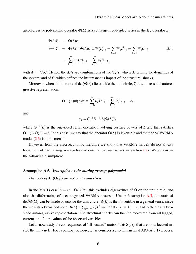
However, from the macroeconomic literature we know that VARMA models do not alwayshave roots of the moving average located outside the unit circle (see Section 2.2). We also makethe following assumption:
Assumption A.5. Assumption on the moving average polynomial
The roots of det(Θ(z)) are not on the unit circle.
In the MA(1) case Yt = (I−ΘL)Cηt , this excludes eigenvalues of Θ on the unit circle, andalso the differencing of a cointegrated VARMA process. Under Assumption A.5, the roots ofdet(Θ(L)) can be inside or outside the unit circle; Θ(L) is then invertible in a general sense, sincethere exists a two-sided series B(L) = ∑
∞k=−∞
BkLk such that B(L)Θ(L) = I, and Yt then has a two-sided autoregressive representation. The structural shocks can then be recovered from all lagged,current, and future values of the observed variables.
Let us now study the consequences of “ill-located” roots of det(Θ(z)), that are roots located in-side the unit circle. For expository purpose, let us consider a one-dimensional ARMA(1,1) process:
6

Dynamic Linear Model and Non-Fundamentalness
(1−ϕL)yt = (1−θL)εt , (2.5)
where |ϕ|< 1 and |θ |> 1.We have:
yt = (1−ϕL)−1(1−θL)εt , (2.6)
and, therefore, yt is a function of the present and past values of εt .To get the (infinite) pure autoregressive representation of process (yt), we have to invert 1−θL.
This leads to:
(1−ϕL)yt =
(1− 1
θL−1)(−θLεt)
⇔(
1− 1θ
L−1)−1
(1−ϕL)yt =−θLεt . (2.7)
Formula (2.7) implies that εt is a function of the future values of yt . Therefore, εt is not thecausal innovation of yt , defined by yt −E(yt |yt−1,yt−2, . . .), the latter being a function of presentand past values of yt only. Formula (2.6) shows that the knowledge of {εt ,εt−1, . . .} implies theknowledge of {yt ,yt−1, . . .}, but since (2.7) shows that εt is not a function of {yt ,yt−1, . . .}, it comesthat the information set {yt ,yt−1, . . .} is strictly included in the information set {εt ,εt−1, . . .}.
To summarize, under Assumptions A.1–A.4, the error term in the VARMA representation isequal to the causal innovation of the process if the roots of det(Θ(z)) are all outside the unit circle.Under this condition, the process (Yt) has a fundamental VARMA representation.3,4 In this case,at any date t, the information contained in the current and past values of Yt coincides with theinformation contained in the current and past values of εt . Otherwise, if some roots of det(Θ(z))
are inside the unit circle, the VARMA representation is non-fundamental. In the latter case, εt isnot equal to the causal innovation, that is, it is not function of present and past observations of Yt
only.Consider a non-fundamental SSVARMA process (Yt) defined by (2.3). (Yt) admits a funda-
mental representation of the form: Φ(L)Yt = Θ∗(L)ε∗t ,5 where process (ε∗t ) is a weak white noise,
3See e.g. Hansen and Sargent (1980), p18, (1991), p79, and Lippi and Reichlin (1994) for the introduction of thisterminology in the macroeconometric literature. The term “fundamental” is likely due to Kolmogorov and appears inRozanov (1960), p367, and Rozanov (1967), p56, to define the “fundamental process”, that is, the second-order whitenoise process involved in the Wold decomposition of a weak stationary process.
4The terminology “fundamental” can be misleading, in particular since fundamental shock and structural shockare often considered as equivalent notions (see e.g. the description of the scientific works of Nobel prizes Sargent andSims in Economic Sciences Prize Committee, 2011, or Evans and Marshall, 2011). Moreover in some papers (seeGrassi, Ferroni, and Leon-Ledesma, 2015) a shock is called fundamental if its standard deviation is non-zero.
5 This representation can be obtained from the non-fundamental SVARMA representation by making use of
7

Dynamic Linear Model and Non-Fundamentalness
i.e. ε∗t and ε∗s , t 6= s, are uncorrelated but not independent, except in the Gaussian case. This pro-cess is the linear causal innovation of (Yt) appearing in the Wold representation, but is in generaldifferent from the nonlinear causal innovation, except in special cases, such as the Gaussian case.In any case, it does not coincide with process (Cηt). Now, consider the new (fundamental) pro-cess (Y ∗t ) defined through Φ(L)Y ∗t = Θ∗(L)C∗ηt , where C∗ satisfies V (ε∗t ) =C∗C∗′. Processes (Yt)
and (Y ∗t ) have the same (dynamic) second-order properties. As a result, the estimation methodsfocussing on second-order properties cannot distinguish between Θ∗(L) and Θ(L). However, thedynamic responses of Yt and Y ∗t to changes in ηt resulting from one or the other MA specificationare different.6
2.2 Examples of non-fundamentalness
There exist different sources of non-fundamentalness in SVARMA models, that is, of “ill-located”roots of the moving average polynomial (see also the discussion in Alessi, Barigozzi, and Capasso,2011). Let us consider some examples and highlight, in each case, the errors with a structuralinterpretation.
i) Lagged impact. A first example of non-fundamentalness is the one provided by Lippi andReichlin (1993) in their comment of the model estimated by Blanchard and Quah (1989).Suppose that the productivity process, denoted by yt , is given by:
yt = εt +θεt−1,
where εt denotes the productivity shock, reflecting for instance the introduction of a techno-logical innovation. It may be realistic to assume that the maximal impact of the productivityshock is not instantaneous and is maximal with a lag, i.e. θ > 1. The MA(1) process is thennon-fundamental (or non-invertible).
ii) Advanced indicator (noise / news shocks). The non-invertibility of the process may also arisefrom some modelling of the information structure. Consider a process (xt) that summarizes
Blaschke matrices. Consider a square matrix of the lag operator denoted by B(L). B(L) is a Blaschke matrix ifand only if [B(L)]−1 = B∗(L−1), where B∗(.) is obtained from B(.) by transposing and taking conjugate coefficients.See Leeper, Walker, and Yang (2013), p1123-1124 for a practical use of Blaschke matrices.
6This is easily illustrated in the context of a univariate MA(1) process. Consider for instance the MA(1) processes(yt) and (y∗t ) respectively defined by yt = σηt − θσηt−1 and y∗t = σθηt −σηt−1. Although (yt) and (y∗t ) have thesame second-order properties, they react differently to shocks to ηt . Consider a one-unit increase in ηt . Whereas thisshock implies increases in yt , yt+1 and yt+h, h > 1, by σ , −θσ and 0, respectively, it implies increases in y∗t , y∗t+1and y∗t+h by σθ , −σ and 0. In particular, if one of these two IRFs is decreasing (in absolute values), the other ishump-shaped.
8

Dynamic Linear Model and Non-Fundamentalness
“fundamentals”, which themselves capture changes in technology, preferences, endowments,or government policy (Chahrour and Jurado, 2018). The dynamics of (xt) is described by:
xt = a(L)ut , (2.8)
where process (ut) is a strong white noise. On date t, the consumer observes xt as well as a“noisy” signal about the future value of fundamentals:
st = xt+1 + vt , (2.9)
where (vt) is also a strong white noise, independent of (ut). This second equation describesthe incremental information about future fundamentals (Barsky and Sims, 2012). If theeconometrician also observes the signal, the model leads to the following bivariate movingaverage representation: [
xt
st
]=
[La(L) 0a(L) 1
][ua
t
vt
], (2.10)
where uat = ut+1.
The determinant of the moving average polynomial has a root equal to zero, which is withinthe unit circle. The moving average representation is therefore non-fundamental. The noiseshock vt has the nature of a demand shock: although it has no effect on fundamentals, itmay affect the macroeconomy because it affects beliefs about future fundamentals throughthe signal st .7 Hence, the existence of this noise may be used to account for belief-drivenbusiness cycles (see e.g. Forni, Gambetti, Lippi, and Sala, 2017b).
This type of analysis is also employed in models disentangling the permanent and transi-tory shocks affecting fundamentals (Lorenzoni, 2009; Blanchard, L’Huillier, and Lorenzoni,2013), or own agent productivity and noisy signal on the aggregate productivity (Lorenzoni,2009, Section 3). Chahrour and Jurado (2018) have recently shown that the previous kind of“noise representation” closely relates to the so-called “news representation”, where peopleperfectly observe part of an exogenous fundamental in advance.8
iii) Rational expectations. Other sources of non-fundamentalness are the rational expectationsintroduced in the models. In the simple example of Hansen and Sargent (1991) the economic
7The “noise” terminology can be misleading: although “noise” mainly refers to vt in this literature, both types ofdisturbances (ut and vt ) are strong white noises, i.e. sequences of i.i.d. variables.
8Basic references on the impacts of “news/noise” shocks include (Blanchard, L’Huillier, and Lorenzoni, 2013;Forni, Gambetti, Lippi, and Sala, 2017a,b; Chahrour and Jurado, 2018).
9

Dynamic Linear Model and Non-Fundamentalness
variable yt is defined as:
yt = Et
(∞
∑h=0
βhwt+h
), with wt = εt−θεt−1, 0 < β < 1, |θ |< 1.
If the information set available to the economic agent at date t is It = (εt ,εt−1, . . .), we get:
yt = (1−βθ)εt−θεt−1.
The root of the moving average polynomial is (1−βθ)/θ . Depending on the values of β andθ , the absolute value of this root is larger or smaller than 1. When the root is strictly smallerthan 1, the model is non-fundamental. In such rational expectation models, the informationsets of the economic agent and of the econometrician are assumed to be aligned.
v) Prediction error. When the variable of interest is interpreted as a prediction error, non-fundamentalness may also appear (see Hansen and Hodrick, 1980). For instance if yt isthe price of an asset at t, Et−2yt can be interpreted as the futures price at t−2 (if the agentsare risk-neutral). The spread between the spot price and the futures price is: st = yt−Et−2yt
and, if yt is a fundamental (invertible) MA(2) process: yt = εt +θ1εt−1 +θ2εt−2 = Θ(L)εt ,then st = εt +θ1εt−1 (= Θ1(L)εt) and the spread process is not necessarily fundamental. Forexample if Θ(L) = (1−θL)2 with |θ |< 1, we have Θ1(L) = 1−2θL, which is not invertibleas soon as |θ |> 1/2.
vi) Non-observability. Non-fundamentalness can arise from a lack of observability. Fernandez-Villaverde, Rubio-Ramirez, Sargent, and Watson (2007) give the example of a state-spacerepresentation of the surplus in a permanent income consumption model (see Lof, 2013,Section 3, for another example). The state-space model is of the following type:{
ct = act−1 +(1−1/R)εt , 0 < a < 1,yt = −act−1 +1/Rεt ,
where yt − ct is the surplus, the consumption ct is latent, R > 1 is a constant gross interestrate on financial assets, and εt is an i.i.d. labor income process. From the first equation, wededuce:
ct =(1−1/R)
1−aLεt ,
10

Dynamic Linear Model and Non-Fundamentalness
and, by substituting in the second equation, the dynamics of yt reads:
yt =
[1/R−a
L(1−1/R)1−aL
]εt =
1/R−aL1−aL
εt .
Thus the root of the moving-average lag-polynomial is equal to 1/aR, and it is smaller thanone when aR > 1.9
2.3 The limits of the Gaussian approach
2.3.1 Static identification issue
Let us first consider the popular case of a structural VAR process (SVAR), where Θ(L) = I. TheGaussian SVAR process is defined by:
Φ(L)yt =Cηt ,
where Φ(0) = I, the roots of det(Φ(z)) are outside the unit circle and where the process (ηt) is aGaussian white noise, with E(ηt) = 0 and V (ηt) = I. The model involves two types of parameters:whereas the sequence Φk, k = 1, . . . , p, characterizes the dynamic features of the model, matrix C
defines (static) instantaneous effects.In this case, the dynamic parameters Φ1, . . . ,Φp are characterized by the Yule-Walker equa-
tions; they are therefore identifiable, but the static parameter C is not, since replacing C by CQ,where Q is an orthogonal matrix, leaves the distribution of process (Yt) unchanged. It is the static
identification problem.In order to solve this identification issue, additional short-run, long-run, or sign restrictions
have been imposed in the literature [see e.g. the references in the introduction].10 It turns out that,if at most one of the components of ηt is Gaussian, the identification problem disappears since C isthen identifiable, up to sign change and permutation of its columns. This result, shown by Comon(1994) (Theorem 11) is a consequence of the Darmois-Skitovich characterization of the multivari-ate Gaussian distribution (see Darmois, 1953; Skitovich, 1953; Ghurye and Olkin, 1961). In thiscase, C can be estimated using Independent Component Analysis (ICA) algorithms (see Hyvärinen,Karhunen, and Oja, 2001), or Pseudo Maximum Likelihood techniques (see Gouriéroux, Monfort,
9This reasoning does not hold for a = 1, which is precisely the case considered in Fernandez-Villaverde, Rubio-Ramirez, Sargent, and Watson (2007), where ct and yt are nonstationary co-integrated processes. Indeed their equa-tion (5) assumes the stationarity of the y process and is not compatible with the assumption of a cointegrated model.
10An alternative consists in leaving the linear dynamic framework by considering Markov Switching SVAR [seeLanne, Lütkepohl, and Maciejowska (2010), Lütkepohl (2013), Herwartz and Lütkepohl (2017), Velinov and Chen(2014)]. In this paper we will stay in a pure SVARMA framework.
11

Dynamic Linear Model and Non-Fundamentalness
and Renne, 2017 or Lanne, Meitz, and Saikkonen, 2017). The identifiability of the static parameterC in the non-Gaussian case implies that the recursive approach proposed by Sims, imposing thatC is lower-triangular, cannot be used in general to find independent shocks, but only uncorrelatedshocks.
2.3.2 Dynamic identification issue
Let us now consider the general case of a SVARMA process:
Φ(L)Yt = Θ(L)Cηt ,
where Φ(0) = Θ(0) = I, the roots of det(Φ(z)) lie outside the unit circle, the roots of det(Θ(z))
can be inside or outside the unit circle, and (ηt) is a Gaussian white noise with E(ηt) = 0 andV (ηt) = I.
Let us focus here on the identification of the dynamic parameters Φ and Θ. In the Gaussiancase, the distribution of the stationary process (Yt) depends on the dynamic and static parametersthrough the second-order moments of the process or, equivalently, through the spectral densitymatrix:
f (ω) =1
2πΦ−1(exp iω)Θ(exp iω)CC′Θ(exp−iω)′Φ−1(exp−iω)′. (2.11)
Using the equalities Γh−Φ1Γh−1− ·· ·−ΦpΓh−p = 0, ∀h ≥ q+ 1, with Γh = cov(Yt ,Yt−h), it isreadily seen that the coefficient matrices Φ1, ..., Φp are identifiable from the distribution of pro-cess (Yt) (Gaussian or not), but several sets of coefficients (Θ1, . . . ,Θq,C) yield the same spectraldensity and the same distribution for the process (Yt) in the Gaussian case; the different polynomi-als Θ(L) are obtained from the fundamental one –the one with the roots of det(Θ(z)) outside theunit circle– by use of Blaschke matrices.11 The lack of identification of the dynamic parametersΘ is called the dynamic identification problem. We see in Section 3 that this second identificationproblem also disappears in the non-Gaussian case.
The dynamic identification problem is simply illustrated in the univariate MA(1) model: yt =
σηt−θσηt−1, where (ηt) is a Gaussian white noise with E(ηt) = 0, V (ηt) = 1 and, for instance,0 < θ < 1. If we replace θ by θ ∗ = 1/θ and σ by σ∗ = σθ , we get another process:
y∗t = σ∗ηt−θ
∗σ∗ηt−1
= σθηt−σηt−1,
11See Footnote 5 for the definition of Blaschke matrices.
12

Dynamic Linear Model and Non-Fundamentalness
which is also Gaussian and with the same covariance function as (yt), namely:
Γ0 = σ2(1+θ
2), Γ1 =−θσ2 and Γh = 0, for h≥ 2,
and, therefore, with the same distribution. In other words, the pairs (θ ,σ) and (1/θ ,σθ) give thesame distributions for processes (yt) and (y∗t ). By contrast, we will see that, if ηt is non-Gaussian,the distributions of processes (yt) and (y∗t ) are different, although their spectral density matricesare the same (see e.g. Weiss, 1975; Breidt and Davis, 1992; Lii and Rosenblatt, 1992).
Alternatively, the process (η∗t ) defined by yt = σθη∗t −ση∗t−1 ≡ σ∗(η∗t − 1θ
η∗t−1), with σ∗ =
σθ is another Gaussian white noise with zero mean and unit variance. More generally in the MA(q)case, yt = θ(L)σηt , with θ(0) = 1, we get other representations (i) by replacing θ(L) by θ ∗(L),where the latter is obtained from θ(L) by inverting some roots (the complex roots being invertedby pairs), and (ii) by replacing σ by σ∗, where the value of σ∗ is determined to give the samemarginal variance to yt . Then the processes (η∗t ) defined through yt = θ ∗(L)σ∗η∗t are Gaussianwhite noises with zero mean and unit variance. Among all these equivalent representations, a singleone is fundamental. In the non-Gaussian case, if one of these (η∗t ) processes is a strong whitenoise, i.e. a serially independent process, the others will be only weak white noises, i.e. seriallyuncorrelated (see Proposition 1 below). If the strong white noise process does not correspond tothe fundamental representation, the weak white noise corresponding to the invertible polynomialθ ∗(L) is the linear innovation process associated with the Wold representation.
In the usual Box-Jenkins approach, the estimation of the parameters Φ1, ..., Φp, Θ1, ..., Θq, Σ =
CC′ is based on a truncated VAR approximation relying on the assumption that Θ(L) is invertible(i.e. the roots of det(Θ(z)) are outside the unit circle), namely a truncation of Θ(L)−1Φ(L)Yt = εt ,with V (εt) = Σ = CC′ (see e.g. Galbraith, Ullah, and Zinde-Walsh, 2002). In other words, a fun-damental representation is a priori imposed without being tested. The introduction of multivariatenon-fundamentalness tests is actually very recent (see e.g. Forni and Gambetti, 2014; Chen, Choi,and Escanciano, 2017).12
12The test developed by Chen, Choi, and Escanciano (2017) exploits the non-normality of the shocks; Forni andGambetti (2014) use information not included in the VAR specification.
13

Identification and Impulse Response Functions (IRFs) in the Non-Gaussian SSVARMA
3 Identification and Impulse Response Functions (IRFs) in theNon-Gaussian SSVARMA
3.1 Identification of the parameters
Consider again the SSVARMA process:
Φ(L)Yt = Θ(L)Cηt ,
and assume that Assumptions A.1 to A.5 hold. Since Φ(L) is invertible, we have:
Yt = Φ−1(L)Θ(L)Cηt = A(L)ηt , (3.1)
with A(L) = Φ−1(L)Θ(L)C.
In Subsection 2.3.1, we have seen that Φ1, . . . ,Φp are characterized by the Yule-Walker equa-tions; they are therefore identified. What about Θ(L) and C? The next proposition is deduced fromTheorem 1 in Chan, Ho, and Tong (2006) (based on Theorem 4 in Chan and Ho, 2004), and solvesthe dynamic identification issue in the non-Gaussian case.13,14 Let us first introduce the followingassumption:
Assumption A.6. Each component of ηt has a non-zero rth cumulant, with r ≥ 3, and a finite
moment of order s, where s is an even integer greater than or equal to r.
Assumption A.6 is introduced to eliminate the Gaussian framework in which all cumulants oforder r ≥ 3 are zero. More precisely, if the true distribution of η j,t has moments of any order, theonly distribution that does not satisfy Assumption A.6 is the Gaussian distribution. Assumption A.6is also satisfied for asymmetric distributions, that is, if the true distribution of η j,t has a non-zeroskewness (and has a finite moment of order 4), or if it is symmetric, but has a non-zero (finite) ex-cess kurtosis. This includes the Student distributions with degrees of freedom strictly larger than 4.
Proposition 1. Under Assumptions A.1 to A.6, if we consider another stationary process (Y ∗t )
defined by:
Φ(L)Y ∗t = Θ∗(L)C∗η∗t ,
13See Findley (1986), Cheng (1992) for the one-dimensional case.14A similar identification result has been recently derived when the components of ηt have fat tails (see Gouriéroux
and Zakoian, 2015).
14

Identification and Impulse Response Functions (IRFs) in the Non-Gaussian SSVARMA
then the processes (Yt) defined in (2.3) and (Y ∗t ) are observationally equivalent if and only if:
Θ(L) = Θ∗(L) and C =C∗,
where the last equality holds up to a permutation and sign change of the columns and η∗t = ηt in
distribution up to the same permutation and sign change of their components.
Proof: See Appendix A.
In order to transform the local identifiability of C under Assumptions A.1 to A.6 into a globalidentifiability, we add the following normalization:15
Assumption A.7. The components of the first row of C are nonnegative and in increasing order.
Proposition 1 provides conditions under which the SSVARMA parameterization is identified.This identification result is however not constructive and does not explain how to estimate thecorrect –possibly non-fundamental– SSVARMA representation.16 This task is the objective of themethods presented in Section 4 below.
3.2 Identification of the structural shocks and of the IRFs
What precedes implies that, under Assumptions A.1 to A.7, the structural shocks ηt are identified.Indeed, we have ηt = C−1Θ−1(L)Φ(L)Yt where, under these assumptions, Φ(L), Θ(L) and C areidentified. The only remaining problem is the labelling of these shocks, since these shocks areordered by Assumption A.7, but not yet interpreted. The labelling will depend on the dynamicimpact of these shocks on the different endogenous variables considered in the model, that is onthe Impulse Response Functions (IRFs). This is completely different from standard structural ap-proaches where the identification of the shocks themselves necessitates additional theory-basedrestrictions. Proposition 1 states that, under Assumptions A.1 to A.7, such restrictions are over-identifying restrictions.
The IRFs are also identified under Assumptions A.1 to A.7 since, in our linear setting, the IRFscorrespond to the coefficients of the MA representation (2.4), which are deduced from Θ(L), Φ(L)
15This normalization is an alternative to the one proposed by Lanne, Meitz, and Saikkonen (2017) in the context ofnon-Gaussian SSVAR (see their Subsection 3.3).
16Theorem 1 of Chen, Choi, and Escanciano (2017) is closely related to Proposition 1. Chen, Choi, and Escanciano(2017) exploit their Theorem 1 to define a test aimed at checking if the fundamental representation is the right one.They do not explain how to estimate the SSVARMA representation under non-fundamentalness.
15

Estimation of Models with Non-Fundamentalness
and C. Specifically, let us denote by IRFj,h the differential impact of a unit shock on η j,t on Yt,h,that is:17
IRFj,h = E(
Yt+h|η j,t = 1,ηt−1
)−E
(Yt+h|ηt−1
), (3.2)
where ηt−1 = {ηt−1,ηt−2, . . .}. Then, from (2.4), we have:18
IRFj,h = ΨhC j, (3.3)
where C j denotes the jth column of matrix C.Equation (3.3) highlights that the IRFs hinge on the fundamentalness regime of the SVARMA
model. It shows indeed that the IRF depends on the (possibly non-invertible) MA coefficientsthrough the Ψh’s.19
Besides, note that IRFj,h can be written ΨhCE(ηt |η j,t = 1) using the serial independence of theηt’s only. Consequently, although the assumption of instantaneous zero correlation is not sufficient,we also get IRFj,h = ΨhC j under the weaker assumption of mean independence (E(ηi,t |η j,t) = 0,∀i 6= j). However, the result of Proposition 1 on the identification of C – and therefore of the IRFs– is based on the assumption of instantaneous independence of the η j,t’s; it has not been shownunder the assumption of mean independence.
4 Estimation of Models with Non-Fundamentalness
In this section, we present parametric and semi-parametric estimation approaches to estimate (pos-sibly) non-fundamental SSVARMA models. For a parametric SSVARMA model, we show that theparameters can be estimated by Maximum Likelihood (ML). More precisely, we explain how tocompute a truncated log-likelihood function. Under regularity assumptions, the estimator resultingfrom the maximization of the latter function achieves asymptotic efficiency. When the distributionof the errors is left unspecified, we propose a two-step approach whose second step is based onmoment restrictions. These restrictions pertain to moments of order higher than three. This semi-parametric approach, which also gives consistent and asymptotically normal estimators, is robustto a misspecification of the error distribution.
17Other IRF definitions can be found in the literature. In particular, Koop, Pesaran, and Potter (1996) discuss the fol-lowing “traditional” definition: E
(Yt+h|ηt+h = 0, . . . ,ηt+1 = 0,ηt = e j,ηt−1
)− E
(Yt+h|ηt+h = 0, . . . ,ηt = 0,ηt−1
).
In the linear case, these “traditional” IRFs are equivalent to those resulting from (3.2), called Generalized IRF (Koop,Pesaran, and Potter, 1996; Pesaran and Shin, 1998).
18If the SSVARMA is non-fundamental, then ηt−1 is not a function of Yt−1, and, therefore, is not observable (even ifthe parameters were known). This is however not a problem for the computation of IRFj,h since, thanks to the linearityof the model and the serial independence assumptions, ηt−1 does not appear in IRFj,h.
19Footnote 6 shows for instance that, in the MA(1) case, if the IRF associated with the fundamental representationis monotonously decreasing, then the one associated with the non-fundamental representation is hump-shaped.
16
Estimation of Models with Non-Fundamentalness
When the dimension of the vector of endogenous variables Yt increases, the number of param-eters specifying the SSVARMA representation (2.3) increases at a much faster rate, giving rise to acurse of dimensionality problem. As a result, in practice, there is a tradeoff between the dimensionn and the degrees p and q in VARMA modelling. Contrary to our ML approach, the numericalcomplexity of the semi-parametric approach does not depend on the autoregressive order p (be-cause the estimate of Φ(L) results from linear regressions). Nevertheless, both methods are subjectto the curse of dimensionality when augmenting the moving-average order q. In most applications,q is equal to 0, 1 or 2. In the following, we focus on VARMA(p,1) models. Subsection 4.1.4 detailshow to extend the ML approach to the estimation of VARMA(p,q) models with q > 1.
4.1 Maximum Likelihood estimation of parametric SSVARMA models
For illustrative purpose, we will first discuss the case of a one-dimensional MA(1) process be-fore considering the general framework of a SSVARMA process. Derivations of truncated log-likelihood functions and associated asymptotic results of ML estimators in the context of possiblynoninvertible univariate MA(q) and ARMA(p,q) processes can notably be found in Lii and Rosen-blatt (1992, 1996), or Wu and Davis (2010). The approach exposed below extends the previousstudies to the multivariate case.
4.1.1 The Maximum Likelihood approach in the MA(1) context
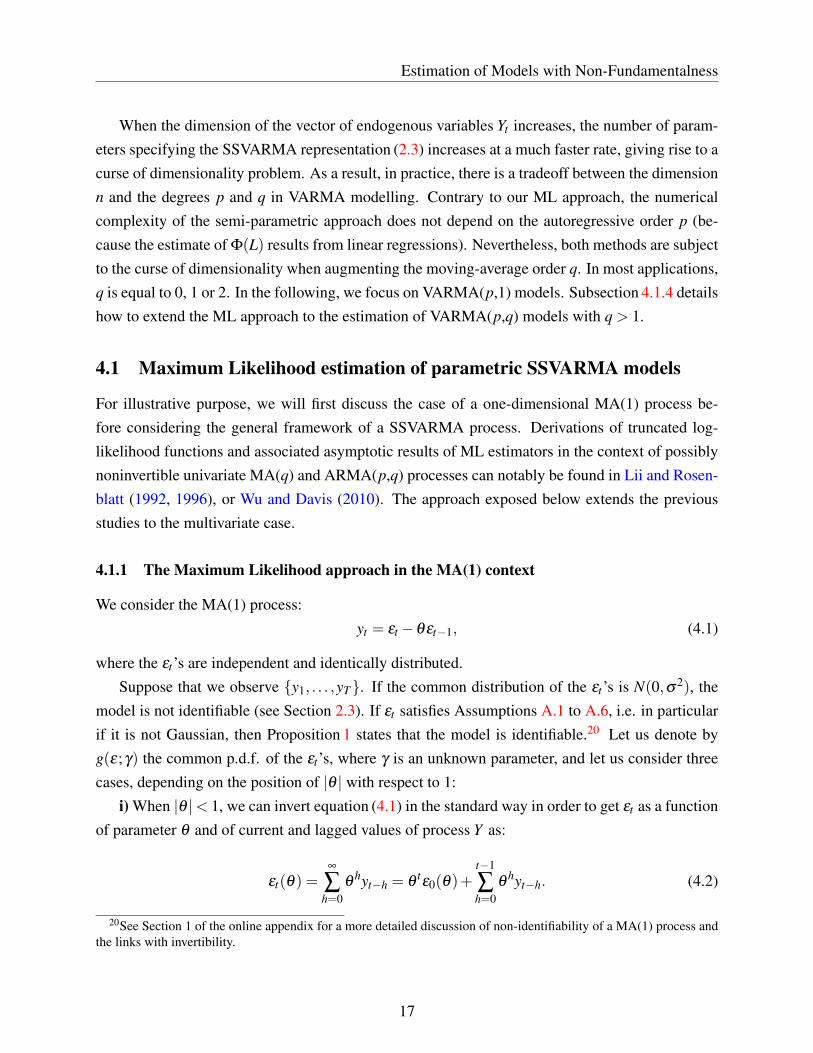
We consider the MA(1) process:yt = εt−θεt−1, (4.1)
where the εt’s are independent and identically distributed.Suppose that we observe {y1, . . . ,yT}. If the common distribution of the εt’s is N(0,σ2), the
model is not identifiable (see Section 2.3). If εt satisfies Assumptions A.1 to A.6, i.e. in particularif it is not Gaussian, then Proposition 1 states that the model is identifiable.20 Let us denote byg(ε;γ) the common p.d.f. of the εt’s, where γ is an unknown parameter, and let us consider threecases, depending on the position of |θ | with respect to 1:
i) When |θ |< 1, we can invert equation (4.1) in the standard way in order to get εt as a functionof parameter θ and of current and lagged values of process Y as:
εt(θ) =∞
∑h=0
θhyt−h = θ
tε0(θ)+
t−1
∑h=0
θhyt−h. (4.2)
20See Section 1 of the online appendix for a more detailed discussion of non-identifiability of a MA(1) process andthe links with invertibility.
17
Estimation of Models with Non-Fundamentalness
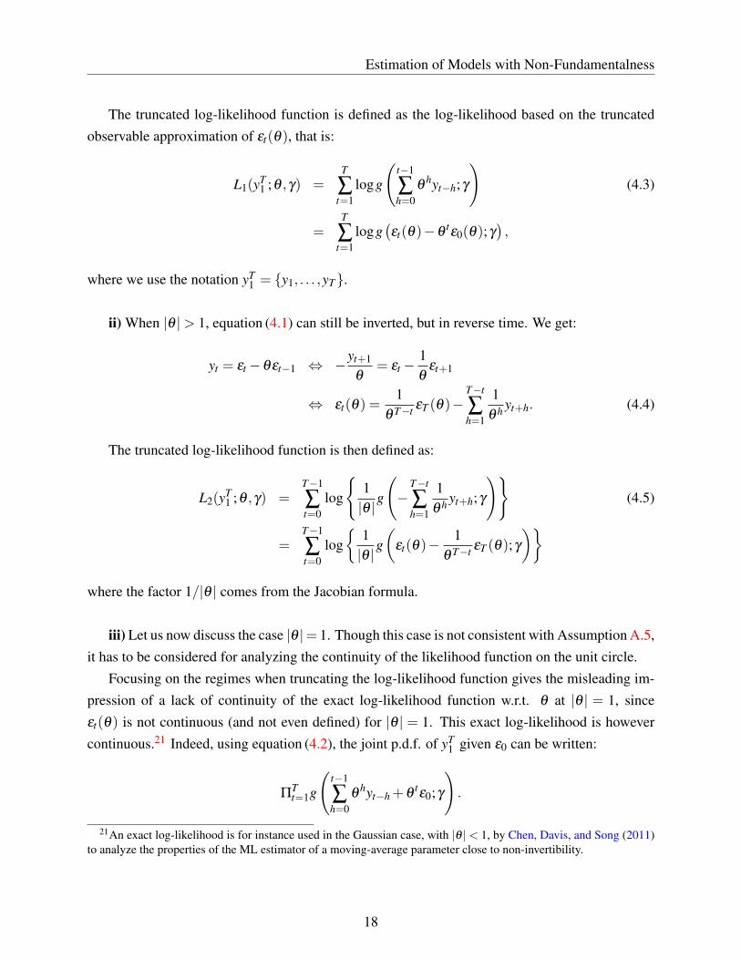
The truncated log-likelihood function is defined as the log-likelihood based on the truncatedobservable approximation of εt(θ), that is:
L1(yT1 ;θ ,γ) =
T
∑t=1
logg
(t−1
∑h=0
θhyt−h;γ
)(4.3)
=T
∑t=1
logg(εt(θ)−θ
tε0(θ);γ
),
where we use the notation yT1 = {y1, . . . ,yT}.
ii) When |θ |> 1, equation (4.1) can still be inverted, but in reverse time. We get:
yt = εt−θεt−1 ⇔ −yt+1
θ= εt−
1θ
εt+1
⇔ εt(θ) =1
θ T−t εT (θ)−T−t
∑h=1
1θ h yt+h. (4.4)
The truncated log-likelihood function is then defined as:
L2(yT1 ;θ ,γ) =
T−1
∑t=0
log
{1|θ |
g
(−
T−t
∑h=1
1θ h yt+h;γ
)}(4.5)
=T−1
∑t=0
log{
1|θ |
g(
εt(θ)−1
θ T−t εT (θ);γ
)}where the factor 1/|θ | comes from the Jacobian formula.
iii) Let us now discuss the case |θ |= 1. Though this case is not consistent with Assumption A.5,it has to be considered for analyzing the continuity of the likelihood function on the unit circle.
Focusing on the regimes when truncating the log-likelihood function gives the misleading im-pression of a lack of continuity of the exact log-likelihood function w.r.t. θ at |θ | = 1, sinceεt(θ) is not continuous (and not even defined) for |θ | = 1. This exact log-likelihood is howevercontinuous.21 Indeed, using equation (4.2), the joint p.d.f. of yT
1 given ε0 can be written:
ΠTt=1g
(t−1
∑h=0
θhyt−h +θ
tε0;γ
).
21An exact log-likelihood is for instance used in the Gaussian case, with |θ |< 1, by Chen, Davis, and Song (2011)to analyze the properties of the ML estimator of a moving-average parameter close to non-invertibility.
18

Estimation of Models with Non-Fundamentalness
Since the distribution of ε0 is g(ε0;γ), the exact log-likelihood is:
L (yT1 ;θ ,γ) = log
{∫Π
Tt=1g
(t−1
∑h=0
θhyt−h +θ
tε;γ
)g(ε;γ)dε
}. (4.6)
Hence, the exact log-likelihood is generally a differentiable function of θ . By contrast, the trun-cated log-likelihood function, given by:
L(yT1 ;θ ,γ) = L1(yT
1 ;θ ,γ)1|θ |<1 +L2(yT1 ;θ ,γ)1|θ |≥1, (4.7)
is only right-differentiable at θ = 1 (and left-differentiable at θ =−1).
In the simple MA(1) case, the maximum likelihood estimation is conducted by directly max-imizing the truncated log-likelihood function (4.7). If |θ | 6= 1, the standard asymptotic theoryapplies (see Proposition 2 below).
4.1.2 The SSVARMA(p,1) case
Let us consider the SSVARMA(p,1) model:
Φ(L)Yt = εt−Θεt−1, (4.8)
where the errors εt are given by:εt =Cηt , say,
where the ηt are independently, identically distributed, have independent components, and aresuch that E(ηt) = 0 and V (ηt) = I. The distribution of the ηt’s is parameterized with γ , say, whereparameter γ is identifiable from the distribution of η . The p.d.f. of the errors εt is therefore of theform g(ε,Γ), with Γ = (C,γ). We assume that this model satisfies Assumptions A.1 to A.7.
Our objective here is to solve system (4.8) in order to get εt’s as linear combinations of Y T−p+1 =
{Y−p+1, . . . ,YT} and of “state variables” – similar to ε0 in (4.2) and to εT in (4.4) – that are such thatsmall changes in these “state variables” only have a small influence on these linear combinationsfor t sufficiently far from the sample bounds (1 and T ). For expository purpose, we denote thesesolutions by εt , without explicitly mentioning their dependence on parameters Φ1, . . . , Φp, Θ, andon observable variables.
19

Estimation of Models with Non-Fundamentalness
Our approach makes use of the real Schur decomposition of matrix Θ:22
Θ = AΘUΘA′Θ = AΘ
UΘ1 UΘ
1,2 . . . UΘ1,K
0 UΘ2 UΘ
2,3 . . . UΘ2,K
... . . . . . . ...0 UΘ
K−1 UΘK−1,K
0 . . . 0 UΘK
A′Θ, (4.9)
where AΘ is orthogonal, UΘ is upper block-triangular, and the diagonal blocks (UΘ
k , k ∈ {1, . . . ,K})are either 1× 1, or 2× 2 blocks, the 2× 2 blocks corresponding to complex conjugate complexeigenvalues of Θ. Under Assumption A.5, the eigenvalues of UΘ are not on the unit circle. Wedenote by nk the dimension of UΘ
k (with nk ∈ {1,2}). We assume, without loss of generality,that UΘ
1 , . . .UΘs have eigenvalues with modulus strictly larger than 1, whereas UΘ
s+1, . . .UΘK have
eigenvalues with modulus strictly lower than 1.Left-multiplying Φ(L)Yt = εt−Θεt−1 by A−1
Θ= A′
Θ, we get:
Wt = ε∗t −UΘε
∗t−1, (4.10)
where Wt = A′Θ
Φ(L)Yt and ε∗t = A′Θ
εt . Note that both Wt and ε∗t depend on parameters and onobservable variables.
Let us denote by ε∗t(1) and ε∗t
(2) the two vectors that are such that ε∗t = [ε∗t(1)′,ε∗t
(2)′]′. Thedimension of ε∗t
(1), that is the non-fundamentalness order, is equal to m = n1 + · · ·+ ns. Thefundamentalness order is equal to n−m. In the same way, we define Wt
(1) and Wt(2) that are such
that Wt = [Wt(1)′,Wt
(2)′]′, Wt(1) being of dimension m.
With a clear block decomposition of UΘ, equation (4.10) writes:[ε∗t
(1)
ε∗t(2)
]=
[Wt
(1)
Wt(2)
]+
[U (1)
ΘU (12)
Θ
0 U (2)Θ
][ε∗t−1
(1)
ε∗t−1(2)
],
22One could also use the real Jordan decomposition for this purpose. Formulas would then actually be slightlysimpler. However, the real Jordan decomposition is less commonly available in programming softwares (typicallyin R). The relative numerical instability of the real Jordan decomposition may account for its absence from usualpackages (see e.g. Söderlind, 1999).
20

Estimation of Models with Non-Fundamentalness
which leads to:
ε∗t(2) = W (2)
t +U (2)Θ
W (2)t−1 + · · ·+U (2)
Θ
t−1W (2)
1 +U (2)Θ
tε∗0(2) (4.11)
ε∗t(1) =
{(U (1)
Θ)−1}T−t
ε∗T(1)− (U (1)
Θ)−1W (1)
t+1−·· ·−{(U (1)
Θ)−1}T−t
W (1)T
−(U (1)Θ
)−1U (12)Θ
ε∗t(2)−·· ·−
{(U (1)
Θ)−1}T−t
U (12)Θ
ε∗T−1
(2). (4.12)
Equation (4.11) shows that, once ε∗0(2) is known, the ε∗t
(2)’s can be computed by forward re-cursions. Since the eigenvalues of U (2)
Θare strictly smaller than one, the effect of the “initial state
variable” ε∗0(2) tends to zero when t tends to infinity. The truncated version of ε∗t
(2) is
ε∗t(2)−U (2)
Θ
tε∗0(2) =W (2)
t +U (2)Θ
W (2)t−1 + · · ·+U (2)
Θ
t−1W (2)
1 . (4.13)
The right-hand side of the previous equation demonstrates that this truncated version of ε∗t(2) de-
pends on model parameters and on observed variables only.Equation (4.12) shows that ε∗t
(1) linearly depends on {W (1)t+1, . . . ,W
(1)T }, on {ε∗t (2), . . . ,ε∗T−1
(2)}and on ε∗T
(1). Since the eigenvalues of (U (1)Θ
)−1 are strictly smaller than one, the effect of the “endstate variable” ε∗T
(1) tends to zero when T − t tends to infinity. The truncated version of ε∗t(1) is
obtained by omitting the term in ε∗T(1) and by replacing the ε∗t+k
(2)’s, k = 0, . . . ,T −1− t, by theirtruncated versions. This truncated version of ε∗T
(1), which depends on model parameters and onobserved variables only, is equal to:
ε∗t(1)−
{(U (1)
Θ)−1}T−t
ε∗T(1)+
(U (1)Θ
)−1[U (12)
Θ+ · · ·+
{(U (1)
Θ)−1}T−t−1
U (12)Θ
U (2)Θ
T−t−1]
︸ ︷︷ ︸≡BΘ,T−t
U (2)Θ
tε∗0(2). (4.14)
Hence, while εt is given by:εt = AΘε
∗t ,
its truncated version is:
AΘ
ε∗t −
{(U (1)Θ
)−1}T−t
ε∗T(1)+BΘ,T−tU
(2)Θ
tε∗0
(2)
U (2)Θ
tε∗0
(2)
= AΘε
∗t −AΘ
{(U (1)Θ
)−1}T−t
BΘ,T−tU(2)Θ
t
0 U (2)Θ
t
[ ε∗T(1)
ε∗0(2)
]. (4.15)
21

Estimation of Models with Non-Fundamentalness
Note that for any value of Θ such that there is no eigenvalue of UΘ on the unit circle, processesεt and ε∗t –seen as functions of the observed variables and of model parameters– are strictly sta-tionary.
The online appendix develops (4.11) and (4.12) in the bivariate VMA(1) case; in this simplecase, one can notably investigates the conditions under which a (structural) shock of interest canbe approximated by means of a VAR model (see Sims, 2012; Forni and Gambetti, 2014; Beaudry,Fève, Guay, and Portier, 2015).
4.1.3 Truncated Maximum Likelihood estimator in the SSVARMA(p,1) case
As in the univariate case (Subsection 4.1.1), we base the definition of the truncated log-likelihoodon the truncated version of εt . For convenience, we denote by Λ = {Φ1, . . . ,Φp,Θ,Γ} the param-eter to be estimated, with Λ ∈L , where L is the parameter set. The truncated log-likelihood isobtained by applying the Jacobian formula. The form of the Jacobian is derived in Appendix B.2.We get the following truncated log-likelihood expression:
LT (Λ) = −Tn
∑i=1
log |λi(Θ)|1|λi(Θ)|>1
+T
∑t=1
logg
AΘε∗t −AΘ
{(U (1)Θ
)−1}T−t
BΘ,T−tU(2)Θ
t
0 U (2)Θ
t
[ ε∗T(1)
ε∗0(2)
];Γ
,(4.16)
where λi(Θ) is the ith eigenvalue of Θ and where the ε∗t are functions of parameter Λ and ofobservations.
The truncated maximum likelihood estimator is defined as the parameter ΛT = {Φ1, . . . ,Φp,Θ, Γ}that maximizes LT (Λ).
We can also introduce the untruncated log-likelihood defined by:
LuT (Λ) = −T
n
∑i=1
log |λi(Θ)|1|λi(Θ)|>1 +T
∑t=1
logg(AΘε∗t ;Γ) . (4.17)
The untruncated log-likelihood depends on values of Y that are not observed. Nevertheless, inorder to derive the asymptotic properties of the truncated maximum likelihood estimator ΛT , itwill prove useful to consider the solution Λu
T that maximizes the untruncated log-likelihood LuT (Λ).
This solution is called the abstract estimator by Bates and White (1985).
Lemma 1. Under Assumptions A.1 to A.5 and under
(a.1) The parameter set L is compact.
22

Estimation of Models with Non-Fundamentalness
(a.2) For any given non-fundamentalness regime, a Schur decomposition continuous in Θ is se-
lected.
(a.3) The density functions of the error terms ηi,t are strictly positive, differentiable, and such that
the derivative of the log-density is Lipschitz with a Lipschitz coefficient that is a continuous
function of Γ.
(a.4) There exists δ > 2 such that E(|η j,t |δ )< ∞, for i = 1, . . . ,n,
then the difference∣∣∣∣ 1T
LT (Λ)−1T
LuT (Λ)
∣∣∣∣ tends almost surely (a.s.) to zero uniformly on the pa-
rameter set L .
Proof: See Online Appendix, Section 3.
Assumption (a.1) allows for decomposing L as ∪sLs, where Ls is the restriction of L to the
parameters with a given (non)fundamentalness regime.23 Each Ls is itself compact. The numberof nonfundamentalness regimes depends on the dimension of Y . For instance, for n = 2, we have5 regimes: one is purely fundamental, two are purely nonfundamental and the last two are mixed(see Appendix B.1). In each regime s, the nonfundamentalness order m(s) is constant.
Assumptions (a.3) and (a.4) are compatible with a variety of tail magnitudes, in particular (mix-tures of) Gaussian, exponential, Student –with a degree of freedom strictly larger than 3 to satisfy(a.4)– or Pareto tails –with a shape parameter strictly larger than 2 to satisfy (a.4).
The advantage of considering the untruncated log-Likelihood is the possibility to write it withthe notations used by Bates and White (1985), that is:
1T
LuT (Λ)≡
1T
T
∑t=1
qt(Y ;Λ),
where Y denotes the complete trajectory of Yt , from−∞ to +∞, and qt(Y ;Λ) = q0(L−tY ;Λ), whereL denotes the lag operator.24 In particular, the process (qt(Y ;Λ)) is strictly stationary and the meanof qt , if it exists, is independent of time. Then we can directly apply (Bates and White, 1985,Theorem 2.5):
23The partition of the parameter space into regimes is the smallest partition of the parameter space –excluding thoseparameterizations entailing one or several Θ’s eigenvalues of modulus equal to one– with connected components. Inthe bivariate case, this partition can be obtained by taking the preimage of an R2 partition based on the trace anddeterminant of Θ (see Appendix B.1).
24The lag operator is denoted by T in Bates and White (1985), who call it measure-preserving one-to-one operator.
23

Estimation of Models with Non-Fundamentalness
Lemma 2. (Bates and White, 1985, Theorem 2.5)
Under Assumptions A.1 to A.5, (a.1), (a.2) and
(a.5) There exists an integrable function qt(Y ) such that qt(Y ) = q0(L−tY ) and
supΛ∈L
qt(Y,Λ)≤ qt(Y ),
then 1T Lu
T (Λ)−E0(qt(Y ;Λ)) tends almost surely to zero when T tends to infinity, uniformly on L .
Taken together, Lemmas 1 and 2 prove the uniform a.s. convergence of 1T LT (Λ)−E0(qt(Y ;Λ)).
We can then deduce the consistency of both the estimator ΛT and its untruncated version ΛuT by
applying the standard Wald-Jennrich argument (Wald, 1949; Jennrich, 1969), which leads to thefollowing proposition:
Proposition 2. Under Assumptions A.1 to A.7, (a.1) to (a.5) and
(a.6) The true parameter value Λ0 ∈L ,
then ΛT (resp. ΛuT ) converges a.s. to Λ0.
Proof: Indeed ΛT (resp. ΛuT ) converges a.s. to the solution of the limiting optimization problem:
Λ∗0 = argmax
Λ∈LE0 [qt(Y ;Λ)] ,
which, by the identification Assumptions A.5 and A.7, is equal to Λ0.
In the above, we have focused on the proof of the strong consistency of the truncated MLestimator. When the true value Λ0 is in interior of L , it is in the interior of one of the Ls, and theasymptotic normality of the estimator is deduced by standard expansion of the first-order conditionwithin Ls.
4.1.4 Extension to the SSVARMA(p,q) case
If Θ(L) is of order q > 1, one can go back to the previous case. For this, define εt = [ε ′t , . . . ,ε′t−q+1]
′
and Yt = [Y ′t ,01×(n−1)q]′. With these notations, the model reads:
Yt = Φ1Yt−1 + · · ·+ ΦpYt−p +(I− ΘL)εt , with Θ =
Θ1 Θ2 . . . Θq
I 0 . . .
0 I 0 . . .... . . .
0 . . . 0 I 0
, (4.18)
24

Estimation of Models with Non-Fundamentalness
and with Φk = [uu′]⊗Φk, where u is a q-dimensional vector equal to [1,0, . . . ,0]′. The eigenvaluesof Θ are the roots of detΘ(z).
Although the representation (4.18) makes it possible to get approximations of the εt’s, it doesnot imply that (Yt) is a VARMA(p,1) process because the process (εt) is not a white noise.
4.2 Semi-parametric estimation of a non-fundamental SSVARMA model
Let us consider a SSVARMA(p,1) model:
Yt = µ +Φ1Yt−1 + · · ·+ΦpYt−p +C0ηt +C1ηt−1, (4.19)
satisfying Assumptions A.1–A.7. For the sake of notational simplicity, we have replaced C by C0
and −Θ1C by C1. We assume that the roots of the determinant of the autoregressive polynomialare outside the unit circle, but the roots of the determinant of the moving average polynomial maybe inside or outside the unit circle. We denote by f j the common probability density functionof the independent η j,t’s, t = 1, . . . ,T . We have to consistently estimate the (true values of the)parameters µ , Φ1, . . . , Φp, C0, C1 as well as the (true) functional parameters f j, j = 1, . . . ,n. Weconsider below a 2-step moment method.
The first step consists in 2-Stage Least Squares (2SLS) regressions using Yt−2, . . . ,Yt−1−k asinstruments (k ≥ p), exploiting the fact that the latter are independent of Zt =C0ηt +C1ηt−1. Wedenote by µ,Φ1, . . . ,Φp the corresponding 2SLS parameter estimates (see Subsection 5.1 of theOnline Appendix for more details about this 2SLS estimator).
Once µ and Φ are estimated, the associated residuals
Zt ≡ Yt− µ− Φ1Yt−1−·· ·− ΦpYt−p, (4.20)
are consistent approximations of Zt =C0ηt +C1ηt−1. Then, in a second step, we proceed with theestimation of C0 and C1 in a pure moving average framework.25
4.2.1 Moment restrictions for C0, C1
Let us first consider the estimation of the moving average parameters as if the true Zt’s wereobserved (this assumption is relaxed in the next subsection). To address the lack of second-orderidentifiability of C0, C1, the econometric literature has proposed to exploit moments of order 3and/or 4 (see e.g. Bonhomme and Robin, 2009, in the special case C1 = 0, Gospodinov and Ng,
25If C1 = 0, C0 can be directly estimated by ICA (see e.g. Chen, Choi, and Escanciano, 2017; Gouriéroux, Monfort,and Renne, 2017; Lanne, Meitz, and Saikkonen, 2017).
25

Estimation of Models with Non-Fundamentalness
2015, in the one-dimensional case, Lobato and Velasco, 2018, in the one-dimensional case throughbi-spectral and tri-spectral density functions).
Loosely speaking, it is appropriate to consider (cross) moments of order 3 if some componentsη j,t of ηt are skewed (i.e. with non-zero third-order cumulants κ3 j) and it is appropriate to use(cross) moments of order 4 if ηt features kurtotic components (with non-zero fourth-order cumu-lants κ4 j). The description of the moment conditions associated with cumulants is provided inAppendix C.26
This approach leads to a set of moment restrictions:
E [h(Zt ,Zt−1;β )] = 0, (4.21)
whereβ = [vecC0
′,vecC1′,κ31, . . . ,κ3n,κ41, . . . ,κ4n]
′. (4.22)
The calibrated moments concern linear combinations of Zt and Zt−1 such as:
E([u′Zt + v′Zt−1]
2) , E([u′Zt + v′Zt−1]
3) , or E([u′Zt + v′Zt−1]
4) , (4.23)
for different pairs (u,v). We get an infinite set of moment restrictions but, in practice, a finite setof pairs has to be selected (see Section 5). Denoting by r the dimension of h(Zt ,Zt−1;β ), the ordercondition is r ≥ 2n2 +2n. The rank condition is challenging to analyse in the multivariate case.27
In practice, difficulties in inverting the asymptotic covariance matrix of the estimator – derived inSubsection 5.2 of the Online Appendix – constitute a signal of non-identification.
In the spirit of the approach proposed by Lobato and Velasco (2018) who work in the frequencydomain, additional types of moment restrictions might be introduced:28
i) We might consider similar moment restrictions based on a different lag order, i.e. E([u′Zt +
v′Zt−k]2), E([u′Zt + v′Zt−k]
3) or E([u′Zt + v′Zt−k]4) for some k > 1.
ii) We might also consider quantities such as: E([u′Zt + v′Zt−1 +w′Zt−2]2), E([u′Zt + v′Zt−1 +
w′Zt−2]3) or E([u′Zt + v′Zt−1 +w′Zt−2]
4).
These additional moment restrictions are likely to bring additional information when q > 1.
26See Boudt, Cornilly, and Verdonck (2018) or Guay and Normandin (2018) for a counting of up-to-order-4 como-ments in the multivariate static case.
27Existing results are only for ARMA(p,q) processes (Gospodinov and Ng, 2015, Lemma 3, and Lobato and Ve-lasco, 2018, Theorem 1). In Gospodinov and Ng (2015), the conditions pertain to specific cumulants of order p+ q;in Lobato and Velasco (2018), the conditions are on multi-dimensional integrals of spectral densities. Guay and Nor-mandin (2018) have recently derived rank conditions in the context of moment-based estimations of SVAR models.
28The approach of Lobato and Velasco (2018) based on bi-spectral and tri-spectral densities seems difficult to extendin the multivariate framework.
26

Applications
4.2.2 2-step moment method
The first step of our approach, namely the 2SLS estimation, provides us with an estimator ofα = [µ ′,vec(Φ)′]′. The second step of the approach involves the sample counterparts of (4.21),after replacement of Zt by Zt = Yt − µ − Φ1Yt−1− ·· · − ΦpYt−p. In others words, the momentrestrictions (4.21) become:
E [h(zt(α),zt−1(α);β )] = 0, (4.24)
with zt(α) = yt − µ −Φ1yt−1−·· ·−Φpyt−p. In the first step, αT is estimated by IV (see 4.2.1);then βT is estimated by mimimization of a moment-based criterion made precise in Subsection 5.2of the Online Appendix (exploiting Appendix C). This minimization implies that
1T
T
∑t=1
h(zt(αT ),zt−1(αT ); βT )≈ 0.
Subsection 5.2 of the Online Appendix derives the asymptotic accuracy of this 2-step momentestimator.
4.2.3 Nonparametric estimation of the error distribution
Once µ , Φ1, . . . , Φp, C0 and C1 have been estimated, consistent approximations of the errors ηt
are based on the truncated estimates of the ε∗t ’s, obtained by recursively applying equations (4.11)and (4.12) of Subsection 4.1.2 (replacing ε∗0
(2) and ε∗T(1) by zero vectors). The p.d.f. f j can then
be estimated by a kernel density estimator applied to the residuals η j,t , t = 1, . . . ,T .
5 Applications
5.1 Monte Carlo exercises
This subsection illustrates the finite-sample performances of the estimation approaches by meansof Monte-Carlo experiments. Subsections 5.1.1 and 5.1.2 respectively deal with MA(1) and VMA(1)processes.
5.1.1 Univariate case
In this subsection, we focus on MA(1) processes:
yt = εt−θεt−1, (4.25)
where the εt’s are serially independent, E(εt) = 0 and V (εt) = 1.
27

Applications
We consider different sample sizes (T = 100, 200 and 500) and different true distributionsof the errors εt . Four distributions are used: the Gaussian distribution, a mixture of Gaussiandistributions and two Student distributions with respective degrees of freedom of 5 and 10. In allsimulations, we use θ =−2. Hence, data generating processes are non-fundamental.
In order to get the intuition behind our approach, it is instructive to look at the joint distributionof yt and yt−1. Figure 1 displays contour plots associated with these distributions in the contextof the four different distributions used for εt . While the black solid lines correspond to the non-fundamental case, the grey lines represent the (pseudo) distribution that would prevail under thefundamental case, i.e. with θ =−1/2 and V (εt) = 4. In the purely Gaussian case (Panel (a)), thetwo distributions coincide, since the two processes are observationally equivalent. By contrast, inthe other three cases –Panels (b), (c) and (d)– the two distributions are different. The case of themixture of Gaussian distributions is particularly illustrative. For this distribution, and in the non-fundamental case, the shock εt is drawn from N (µ1,σ
21 ) with probability p and from N (µ2,σ
22 )
with probability 1− p. We set: µ1 = −0.7, µ2 = 0.7, σ1 = 0.32, σ2 = 0.95, p = 0.5, whichresults in a zero-mean unit-variance distribution with order-3 and order-4 cumulants of 0.85 and 0,respectively.29
For the ML approach (Subsections 4.1), and for each of the four distributions, we estimate fiveparameters: θ , the variance of εt and three parameters specifying a mixture of Gaussian distri-butions with zero mean and unit variance. As far as the Student distributions are concerned, weproceed under the assumption that we do not know the true distribution, which is generally thecase in practice. Hence, when the true distributions are Student, the ML approach is, more pre-cisely, a Pseudo Maximum Likelihood (PML) approach.30 This exercise is in the spirit of Lii andRosenblatt (1996) and Wu and Davis (2010), who study the performances of their ML estimatorswhen using a misspecified distribution in the computation of the log-likelihood function.
In the context of our variant of the GMM approach (Subsection 4.2), we consider the order-2,order-3 and order-4 moments given in (4.23), with (u,v) ∈ {(1,0),(1,2),(2,1)}.31 Hence, we use9 restrictions to estimate, for each model, the four following parameters: θ , the variance of εt , κ3
and κ4.In our discussion of the results, we focus on the estimates of θ . Figure 2 shows the distributions
of the estimators of θ resulting from both approaches. Each of the four rows of plots corresponds toone of the four considered distributions for εt , that are those distributions represented on Figure 1.
29In their Monte-Carlo experiment, Gospodinov and Ng (2015) also consider a distribution characterized by κ3 =0.85 and κ4 = 0.
30When the true distribution is Gaussian or a Gaussian mixture, the approach is not a PML, but a standard MLapproach. Note that the Gaussian distribution is a special case of Gaussian mixture.
31We do not use (u,v) = (1,1) because, for these values of u and v, the moments of uyt + vyt−1 are the sameas those of vyt + uyt−1, thereby preventing theas identification of the parameters. Indeed, if yt = εt − θεt−1 andy∗t =−θεt + εt−1, then yt + yt−1 and y∗t + y∗t−1 have the same distribution, and therefore the same moments.
28

Applications
On each panel, the three curves correspond to the three considered sample sizes (T = 100, 200 and500). The (finite sample) distributions are often bimodal; one mode being close to the true valueof θ –indicated by a vertical bar on each panel– and the other being close to 1/θ .
The results illustrate the fact that, the closer the distribution of the generated shocks is to anormal one, the weaker the identification. Let us focus for instance on the fraction of estimatedfundamental processes, i.e. with θ estimates that are lower than 1 in absolute value (whereas thedata generating process is non-fundamental since |θ | > 1). In the Gaussian case (Panels a.1 anda.2 of Figure 2), about half of the estimated processes are fundamental, irrespective of the samplesize or of the estimation approach. Among the three remaining distributions, the one leading to thelargest fractions of estimated fundamental processes is the Student t(10). For the latter distributionand in the ML case, even for a relatively large sample size (T = 200), about a third of the estimatedθ ’s have a modulus lower than 1, whereas this proportion is of about 12% in the Student-t(5) caseand close to 0% in the Gaussian mixture case. Identification is easier in the Student t(5) and in theGaussian mixture cases (Panels b.1, b.2, c.1 and c.2) since, in these cases, the differences betweenthe distributions of (yt−1,yt) in the fundamental versus non-fundamental regimes are more markedthan for the other two distributions, as illustrated by Figure 1.
Table 1 reports summary statistics associated with the different estimators. The results showthat our GMM approach is less efficient than the (P)ML one. Indeed, Root Mean Squared Er-rors (RMSEs) are lower with the (P)ML approach. This is the case even when the (P)ML usesa misspecified distribution, i.e. when the true distributions are Student-t. These lower RMSEsare accounted for by far smaller standard deviations of the estimator distributions for the (P)MLapproach, which more than compensates the fact that (P)ML-estimator biases are often larger thanin the GMM case.
To the best of our knowledge, this study is the first one to compare GMM and ML estimatesin the context of non-fundamental univariate MA processes. As regards the GMM approach, ourresults are comparable to the results in the literature, such as the ones reported by Gospodinov andNg (2015) for T = 500, or by Lobato and Velasco (2018) with spectral-density-based estimator forT = 100, 200 and Student t(5) distribution.32
The last two columns of Table 1 aim at assessing the validity of the asymptotic distributionof the θ estimators. These columns indicate the fractions of times (among the N simulations)where the true value of θ lies within the interval [θ − φασasy, θ + φασasy], where σasy denotesthe estimate of the asymptotic standard deviation of the estimator θ and where φα is such that
32Our GMM estimator however appears to be less efficient than the spectral-density-based estimator of Lobato andVelasco (2018): For T = 200 and when the true distribution is t(5), Lobato and Velasco (2018) report that the absolutevalue of their θ estimator is on the right side of 1 in 93% of the cases (last column in their Table 1), while we get anequivalent percentage of 71% with our GMM estimator. This percentage is of 88% for our PML estimator. Our PMLRMSEs are close to those reported by Lobato and Velasco (2018) in this case (T = 200, t(5) distribution, θ =−2).
29

Applications
P(−φα < X < φα) = α , if X ∼ N (0,1). The closer to α the reported fractions, the better theasymptotic approximation of the estimator distribution. For each of the two considered values ofα , two ratios are reported: while the first one is based on all simulated sample paths, the secondone (in italics) excludes those paths where the wrong fundamentalness regime is estimated. Indeed,when the wrong fundamentalness regime is estimated, it is extremely likely that the true value ofθ is not in the estimated confidence interval; this is because σasy does not integrate the fact thatthe wrong fundamentalness regime may have been estimated. As expected, the results indicatethat the adequacy between the ratios and the α’s is better in the second case, that is when theright fundamentalness regime is estimated (the proportion of the latter cases is reported in the sixthcolumn of Table 1). Let us stress that while this second case points to the validity of the asymptoticapproximation of the estimator distribution, it is not consistent with practical situations, where theright fundamentalness regime is usually unknown.
5.1.2 Bivariate case
Let us now consider the following bivariate VMA(1) process:
Yt =Cηt−ΘCηt−1, (4.26)
with
C =
[0 11 0.5
]and Θ =
[−0.5 0
1 −2
]. (4.27)
Both components of ηt are independently drawn. The first structural shock, η1,t , is drawn from amixture of Gaussian distributions featuring a skewness of 2 and an excess kurtosis of 6.33 The sec-ond structural shock, that is η2,t , is drawn from a Student’s distribution with 6 degrees of freedom,i.e. with a skewness of 0 and an excess kurtosis of 3.
For each simulated path of Yt , we implement both the GMM and the ML approaches. Asregards the ML approach, we proceed as if we did not know that the true distribution of η2,t was aStudent’s distribution and we use mixtures of Gaussian distributions for both η1,t and η2,t . Strictlyspeaking, this approach is therefore a PML one. Whereas twelve parameters are estimated inthe GMM case, fourteen are involved in the ML case: both cases involve the estimation of thecomponents of C and Θ (8 parameters); the remaining parameters to be estimated are κ3,i and κ4,i,i∈ {1,2} in the GMM case (where i = 1 for the first structural shock and i = 2 for the second one),and pi, µ1,i and σ1,i, i ∈ {1,2} in the PML case (constrained by the zero mean and unit varianceconditions). For the GMM approach, we consider the order-2, order-3 and order-4 moments given
33 Specifically, thus first shock is drawn from N (µ1,σ21 ) with probability p and from N (µ2,σ
22 ) with probability
1− p, where µ1 = 2.12, µ2 =−0.24, σ1 = 1.41, σ2 = 0.58, p = 0.1.
30

Applications
in (4.23) with:
(u1,u2,v1,v2) ∈ {(2,0,0,0),(0,2,0,0),(1,0,2,0),(2,0,1,0),(1,0,0,2),(2,0,0,1),
(0,1,0,2),(0,2,0,1),(0,1,2,0),(0,2,1,0)} , (4.28)
which results in 30 restrictions.34
Figure 3 shows the densities of the estimators of the Θi, j’s. As in the univariate case, somedistributions are bi-modal, in particular for the shorter samples and for Θ1,1 and Θ2,2. Thesedensities also show that the PML estimates are on average more precise than the GMM ones.Table 2 documents the latter point: its third column indicates in particular that the RMSEs arelower in the PML case. The sixth column reports the fraction of replications for which the “rightfundamentalness regime” is estimated. Here, we consider that an estimated model features the“right fundamentalness regime” if the estimate of Θ has one eigenvalue on each side of the unitcircle and if the absolute values of the estimates of Θ1,1 and Θ2,2 are respectively below and aboveone, as the true values.35 It appears that the PML estimations result in the right fundamentalnessregime in more than 90% of the cases as soon as T is larger than 200. The GMM approach is lesssuccessful, with 67% of correct regime identification for T = 500.
5.2 Bivariate real-data example: GNP growth and unemployment
For comparison with the literature, we consider the two-variable model of Blanchard and Quah(1989), referred to as BQ hereafter. The two stationarized endogenous variables are the U.S. realGNP growth and the (detrended) unemployment rate. BQ fit an 8-lag VAR model to these datafor the period from 1948Q2 to 1987Q4 (159 dates) and impose long-run restrictions to identifydemand and supply shocks. Specifically, they impose that the demand shock has no long-runimpact on real GNP. That is, in their model, the contribution of supply disturbances to the varianceof output tends to unity as the horizon increases.
Using the same dataset and analyzing the location of the (complex roots) of the 8-lag VARof BQ, Lippi and Reichlin (1994)’s results suggest that this VAR approximates a VARMA(1,1)model. Further, Lippi and Reichlin (1994) explore the influence of inverting the roots of the mov-ing average polynomial of this VARMA(1,1) model on the IRFs. They illustrate that fundamentaland non-fundamental versions of the model have different implications, notably in terms of firstimpacts of the shocks and of variance decompositions. However, their analysis does not allowthem to statistically pinpoint the most suitable model among the different versions they obtain (the
34See Footnote 31 for the reason why the ui’s and vi’s are not in {0,1} only.35Because (the true value of) Θ is triangular, its eigenvalues coincide with its diagonal elements. It is not the case
for its estimate.
31
Applications
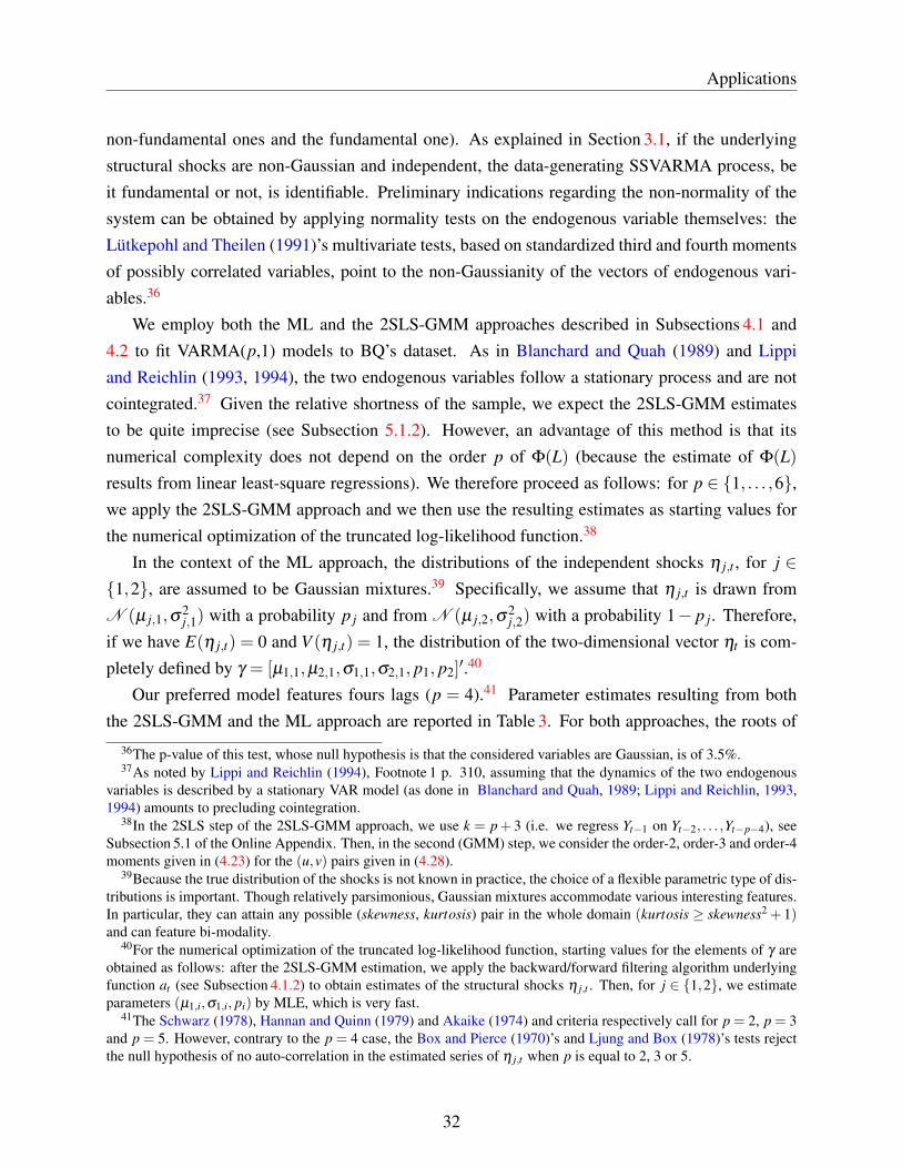
non-fundamental ones and the fundamental one). As explained in Section 3.1, if the underlyingstructural shocks are non-Gaussian and independent, the data-generating SSVARMA process, beit fundamental or not, is identifiable. Preliminary indications regarding the non-normality of thesystem can be obtained by applying normality tests on the endogenous variable themselves: theLütkepohl and Theilen (1991)’s multivariate tests, based on standardized third and fourth momentsof possibly correlated variables, point to the non-Gaussianity of the vectors of endogenous vari-ables.36
We employ both the ML and the 2SLS-GMM approaches described in Subsections 4.1 and4.2 to fit VARMA(p,1) models to BQ’s dataset. As in Blanchard and Quah (1989) and Lippiand Reichlin (1993, 1994), the two endogenous variables follow a stationary process and are notcointegrated.37 Given the relative shortness of the sample, we expect the 2SLS-GMM estimatesto be quite imprecise (see Subsection 5.1.2). However, an advantage of this method is that itsnumerical complexity does not depend on the order p of Φ(L) (because the estimate of Φ(L)
results from linear least-square regressions). We therefore proceed as follows: for p ∈ {1, . . . ,6},we apply the 2SLS-GMM approach and we then use the resulting estimates as starting values forthe numerical optimization of the truncated log-likelihood function.38
In the context of the ML approach, the distributions of the independent shocks η j,t , for j ∈{1,2}, are assumed to be Gaussian mixtures.39 Specifically, we assume that η j,t is drawn fromN (µ j,1,σ
2j,1) with a probability p j and from N (µ j,2,σ
2j,2) with a probability 1− p j. Therefore,
if we have E(η j,t) = 0 and V (η j,t) = 1, the distribution of the two-dimensional vector ηt is com-pletely defined by γ = [µ1,1,µ2,1,σ1,1,σ2,1, p1, p2]
′.40
Our preferred model features fours lags (p = 4).41 Parameter estimates resulting from boththe 2SLS-GMM and the ML approach are reported in Table 3. For both approaches, the roots of
36The p-value of this test, whose null hypothesis is that the considered variables are Gaussian, is of 3.5%.37As noted by Lippi and Reichlin (1994), Footnote 1 p. 310, assuming that the dynamics of the two endogenous
variables is described by a stationary VAR model (as done in Blanchard and Quah, 1989; Lippi and Reichlin, 1993,1994) amounts to precluding cointegration.
38In the 2SLS step of the 2SLS-GMM approach, we use k = p+ 3 (i.e. we regress Yt−1 on Yt−2, . . . ,Yt−p−4), seeSubsection 5.1 of the Online Appendix. Then, in the second (GMM) step, we consider the order-2, order-3 and order-4moments given in (4.23) for the (u,v) pairs given in (4.28).
39Because the true distribution of the shocks is not known in practice, the choice of a flexible parametric type of dis-tributions is important. Though relatively parsimonious, Gaussian mixtures accommodate various interesting features.In particular, they can attain any possible (skewness, kurtosis) pair in the whole domain (kurtosis ≥ skewness2 + 1)and can feature bi-modality.
40For the numerical optimization of the truncated log-likelihood function, starting values for the elements of γ areobtained as follows: after the 2SLS-GMM estimation, we apply the backward/forward filtering algorithm underlyingfunction at (see Subsection 4.1.2) to obtain estimates of the structural shocks η j,t . Then, for j ∈ {1,2}, we estimateparameters (µ1,i,σ1,i, pi) by MLE, which is very fast.
41The Schwarz (1978), Hannan and Quinn (1979) and Akaike (1974) and criteria respectively call for p = 2, p = 3and p = 5. However, contrary to the p = 4 case, the Box and Pierce (1970)’s and Ljung and Box (1978)’s tests rejectthe null hypothesis of no auto-correlation in the estimated series of η j,t when p is equal to 2, 3 or 5.
32

Applications
det(Φ(z)) are outside the unit circle; the estimated processes are therefore stationary. Besides,for both estimation methods, the two roots of det(I−Θz) are on each side of the unit circle (1.77and 0.41 for the ML approach, 2.34 and −0.03 for the GMM approach). Hence, the estimatedprocesses are non-fundamental. Figure 4 shows the ML estimated parametric distributions of thestructural shocks (Gaussian mixtures, represented by dotted lines). These estimated distributionsare fairly close to kernel-based densities associated with the η j,t’s estimates derived from the back-ward/forward filtering algorithm underlying function at , introduced in Subsection 4.1.2.
It is difficult to check ex-ante the relevance of the assumptions on the structural shocks, in par-ticular regarding the independence assumption A.1. Tests can however be applied to the estimatedstructural shocks. In the present case, the application of Box and Pierce (1970)’s and Ljung andBox (1978)’s tests on the estimated series of structural shocks do not detect auto-correlation in theestimated series of η j,t , |η j,t |, nor in the η2
j,t , which is a necessary condition for independence. Thenormality hypothesis of the η j,t’s is rejected by the Shapiro and Wilk (1965)’s test, with p-valuesbelow 2%.42 A limitation of these residual tests is however that they do not take into account theuncertainty regarding the estimation of the η j,t’s; this is left for future research.
Figure 5 displays the impulse response functions resulting from the ML approach and comparesthem with those obtained with long-run restrictions à la Blanchard and Quah (1989). Becausethe ML approach does not rely on restrictions based on economic theory, the resulting structuralshocks have no a priori economic interpretation. However, for comparing the different approaches,we bring the BQ supply shock closer to the ML-estimated shocks that accounts for the largest partof the GNP long-run variance. We call this shock the “long-run shock”.
Figure 5 shows that the BQ and ML response functions present similarities. Nevertheless, inthe ML approach, both structural shocks –Shock 1 (first column of charts) and Shock 2 (secondcolumn of charts)– have a long-run impact on GNP. This is not the case with the BQ approachwhere, by construction, the effect of Shock 1 on GNP converges to zero. The fact that none of thetwo structural shocks identified within a bivariate VAR has a zero impact on output in the long-runwas also obtained by Cochrane (1994) for instance.43 The responses of unemployment to Shock1 (bottom-left plot) and of GNP to Shock 2 (upper-right plot) broadly feature the same shapes forboth approaches, but do not agree on the delay before maximal impact. The bottom-right plotshows that, according to the ML approach, the instantaneous response of unemployment to thesecond (long-run) shock is close to zero, reflecting the fact that the estimated coefficient C2,2 issmall and not statistically different from zero (see Table 3). Obtaining a C coefficient equal to zero
42Because no auto-correlation is detected in the residual, there is no need for using autocorrelation-robust normalitytests such as those of Bai and Ng (2005) and of Lobato and Velasco (2004).
43The bivariate model of Cochrane (1994) describes the joint dynamics of GNP and consumption growth. Thestructural shocks are identified by means of a short-run restriction (consumption does not respond contemporaneouslyto a GNP shock).
33

Concluding remarks
is reminiscent of what could be obtained in the context of an identification strategy à la Sims –imposing that one structural shock has no contemporaneous impact on the unemployment rate.However, the results presented here could not have been obtained in this context since the standardshort-run restriction methodology (à la Sims) is based on VAR models and therefore necessarilyleads to fundamental models. By contrast, our approach remains a priori agnostic with respect tothe fundamentalness regime.
6 Concluding remarks
We have shown in this paper that the static and dynamic identification problems associated withGaussian structural VARMA processes disappear if (i) the structural shocks are non-Gaussian andif (ii) these shocks are serially and instantaneously independent. In other words, non-Gaussianstrong structural VARMA (SSVARMA) models are identified. We further propose parametric andsemi-parametric estimation methods able to consistently estimate possibly non-fundamental repre-sentation in the moving average dynamics. Our analysis also highlights the fact that, in the contextof non-Gaussian SSVARMA, the impulse response functions are defined in a non-ambiguous way.
Conventional econometric toolboxes available to macroeconomists have often been conceivedfor linear forecasting purposes and for SVARMA models with shocks that are uncorrelated, but notindependent. Because it focuses on second-order properties only, the standard SVARMA literatureand associated toolboxes often introduce potentially over-identifying assumptions that may entailmisspecification and misleading interpretation of SVARMA residuals. As shown in the parametricand semi-parametric analysis developed in Section 4 and in the applications presented in Section 5,such potential pitfalls can be addressed in the non-Gaussian case, provided that the independenceassumptions are valid and that the appropriate estimation methods are used.
The methods developed in this paper might be extended in several directions, which are left forfuture research. First testing procedures, in particular tests of fundamentalness, may be obtained.Second the properties of estimation methods can be analyzed in a neighbourhood of the Gaussianassumption (see e.g. Gouriéroux and Jasiak, 2016), or in a neighbourhood of unit roots (see e.g.Chen, Davis, and Song, 2011, for non-invertible MA process). Third, the asymptotic propertiesof our ML estimate in the presence of cointegration may be derived. Fourth, the identificationand estimation results might be extended to the case of more errors than observables. Indeed,while identification results exist when the errors are not Gaussian (see e.g. Th 3.1. in Erikssonand Koivunen, 2004, for the static case, Gouriéroux and Zakoian, 2015, for stable multivariateprocesses, or Gagliardini and Gouriéroux, 2018, for a non-Gaussian factor model), the possibilityto identify the dynamics when the number of shocks is larger than the number of endogenousvariables and the errors are not Gaussian would be important in the discussion of the effect of
34

Proof of Proposition 1
omitted variables (see e.g. Giannone and Reichlin, 2006; Lütkepohl, 2014).
A Proof of Proposition 1
Let us first recall Theorem 1 in Chan, Ho, and Tong (2006).
Theorem. Let Yt and Y ∗t be two non-Gaussian processes defined by:
Yt =∞
∑k=−∞
Akεt−k,
Y ∗t =∞
∑k=−∞
A∗kε∗t−k,
where the processes εt and ε∗t are strong white noises with independent components.
Then, Yt and Y ∗t are observationally equivalent if and only if
ε∗j,t−m( j) = σ jεπ( j),t (equality in distribution), (a.1)
A∗k, j =1σ j
Ak−m( j),π( j), (a.2)
where π is a permutation and Ak, j (respectively A∗k, j) is the jth column of Ak (respectively A∗k)
provided the following condition holds:
the components of εt (resp. ε∗t ) have non-zero rth cumulant, with r ≥ 3 and a finite even
moment of order s greater than, or equal to, r.
If the moving averages are one-sided (Ak = A∗k = 0, ∀k < 0, A0 6= 0,A∗0 6= 0) and εt (resp. ε∗t ) isreplaced by ηt (resp. η∗t ), where the components of ηt (resp. η∗t ) have a unit variance, this impliesthat m( j) = 0 and σ j =±1 for all j.
In our case, we have:
Yt = Ψ(L)Cηt ,
Y ∗t = Ψ∗(L)C∗η∗t ,
with
Ψ(L) = Φ−1(L)Θ(L) = I +Ψ1L+Ψ2L2 + . . . ,
Ψ∗(L) = Φ
−1(L)Θ∗(L) = I +Ψ∗1L+Ψ
∗2L2 + . . .
35

Truncated Maximum Likelihood Approach
Therefore, we have:
Ak = ΨkC with Ψ0 = I,
A∗k = Ψ∗kC∗ with Ψ
∗0 = I.
The previous theorem implies that the moving average matrix coefficients Ak are identified up to apermutation and a sign change of the columns. That is, there exists a permutation matrix P and adiagonal matrix D, whose diagonal elements are either −1 or 1, that are such that:
ΨkC = Ψ∗kC∗PD, ∀ k.
For k = 0, this gives C =C∗PD, which further implies that Ψk = Ψ∗k for all k. The Ψk are thereforeidentified and C is identified up to a permutation and a sign change of its columns. Since Φ(L) andΨ(L) are identified, Θ(L) = Φ(L)Ψ(L) is also identified.
B Truncated Maximum Likelihood Approach
B.1 The nonfundamentalness regimes for n = 2
When n = 2, the eigenvalues of Θ are the solutions of the second-order polynomial equation:
λ2−Tr(Θ)λ +det(Θ) = 0.
Consider the case of roots with modulus equal to one. Three limiting cases have to be considered:
i) One eigenvalue is equal to 1. This arises if 1−Tr(Θ)+det(Θ) = 0.
ii) One eigenvalue is equal to −1. This arises if 1+Tr(Θ)+det(Θ) = 0.
iii) Two complex eigenvalues have a modulus equal to 1. This arises if the second-order poly-nomial equation is of the form: λ 2− 2cos(a)λ + 1 = 0. This implies |Tr(Θ)| < 2 anddet(Θ) = 1.
The three frontiers above define 5 regions, as illustrated on Figure 6: Region I is purely fundamen-tal; Regions III and V are purely nonfundamental; Regions II and IV are mixed. The dashed linerepresents the pairs (Tr(Θ),det(Θ)) for which the discriminant Tr(Θ)2−4det(Θ) is zero; the areathat is below (respectively above) this parabola corresponds to real (resp. complex) eigenvaluesfor Θ.
36

Truncated Maximum Likelihood Approach
B.2 Derivation of the Jacobian
Replacing the ε∗t(2)’s appearing in equation (4.12) by their expressions given in (4.11), one obtains:
ε∗0(1)
...ε∗T−1
(1)
ε∗1(2)
...ε∗T
(2)
︸ ︷︷ ︸
=ε∗
=
[J1 J12
0 J2
]︸ ︷︷ ︸
=J
W1(1)
...WT
(1)
W1(2)
...WT
(2)
︸ ︷︷ ︸
=W
+
{(U (1)
Θ)−1}T
M0...
...
(U (1)Θ
)−1 MT−1
0 U (2)Θ
......
0 (U (2)Θ
)T
︸ ︷︷ ︸
=M
[ε∗T
(1)
ε∗0(2)
], (a.3)
where J1 is an upper block triangular matrix with{−(U (1)
Θ)−1}
matrices on its diagonal, where J2
is lower block triangular with identity matrices on its diagonal, and where:
Mt =−(U (1)Θ
)−1U (12)Θ
(U (2)Θ
)t−·· ·−
{(U (1)
Θ)−1}T−t
U (12)Θ
(U (2)Θ
)T−1
.
Let’s consider the vector V = [V ′1, . . . ,V′T ]′ where Vt = Φ(L)Yt . If Y = [Y ′1, . . . ,Y
′T ]′, we have V =
DY +D0Y 0 where D is a lower triangular matrix whose diagonal is filled with ones (and thereforedetD = 1), where D0 is matrix of dimension (nT )× (np), and where Y 0 = [Y ′0, . . . ,Y
′−p+1]
′.By definition of Wt , we have AΘWt = Φ(L)Yt and, therefore, A′
ΘVt = Wt . Hence, with W =
[W ′1,W′2, . . . ,W
′T ]′, we obtain:
W = (I⊗A′Θ)V = (I⊗A′Θ)(DY +D0Y 0).
Let’s denote by P the permutation that is such that W = PW , where W is defined in equation (a.3).Consider the case where ε∗0
(2) and ε∗T(1), thought of as state variables, are equal to zero. We obtain,
using the notations of equation (a.3):
ε∗ = JW = JPW = JP(I⊗A′Θ)(DY +D0Y 0). (a.4)
Matrices AΘ and P being orthogonal, we have |detAΘ|= |detP|= 1. Since we also have detD = 1,we get:
|det(JP[I⊗A′Θ]D)|= |det(J)|= 1
|det(U (1)Θ
)|T.
Denoting by λi(Θ) the ith eigenvalue of Θ, the effect of the Jacobian on the truncated log-
37

2SLS-GMM: Cumulant-based identification
likelihood is:
log(|det(U (1)Θ
)|) =n
∑i=1
log |λi(Θ)|1|λi(Θ)|≥1. (a.5)
C 2SLS-GMM: Cumulant-based identification
The first step provides consistent estimates of µ , Φ1, . . . ,Φp (see Subsection 5.1 of the OnlineAppendix). Therefore we can focus on the identification and the derivation of moments on thepure VMA process: Zt =C0ηt +C1ηt−1.
The pairwise log-Laplace transform of (Zt ,Zt−1) is:
logE[exp(u′Zt + v′Zt−1)] (a.6)
= logE[exp(u′(C0ηt +C1ηt−1)+ v′(C0ηt−1 +C1ηt−2))]
= log(E[exp(u′C0ηt)]×E{exp[(u′C1 + v′C0)ηt−1]}×E[exp(v′C1)ηt−2]
)=
n
∑j=1
logE[exp(u′C0 jη j,t)]+n
∑j=1
logE{exp[(u′C1 j + v′C0 j)η j,t−1}+n
∑j=1
logE[exp(v′C1 jη j,t−2)],
using that the η j,t’s are mutually and serially independent.Let us denote by Ψξ the log-Laplace transform of a given random variable ξ defined by:
Ψξ (u) = logE[exp(wξ )].
If the moments of ξ exist up to order 4, and if E(ξ )= 0, the log-Laplace transform can be expandedas:
Ψξ (w)≈w2
2E(ξ 2)+
w3
6E(ξ 3)+
w4
24[E(ξ 4)−3E(ξ 2)
]. (a.7)
In particular, for the η j’s, for which E(η j) = 0 and E(η2j ) = 1, we have:
Ψη j(w)≈w2
2+
w3
6κ3 j +
w4
24κ4 j, (a.8)
with κ3 j = E(η3j,t) and κ4 j = E(η4
j,t)−3.Using (a.7) with ξ = u′Zt + v′Zt−1 and (a.8), and taking the expansions of both sides of (a.6)
38

up to order 4, we get the following restrictions, holding for any pair (u,v):
E[(u′Zt + v′Zt−1)2] = ∑
nj=1[(u
′C0 j)2 +(u′C1 j + v′C0 j)
2 +(v′C1 j)2] (order 2)
E[(u′Zt + v′Zt−1)3] = ∑
nj=1 κ3 j[(u′C0 j)
3 +(u′C1 j + v′C0 j)3 +(v′C1 j)
3] (order 3)E[(u′Zt + v′Zt−1)
4] = ∑nj=1 κ4 j[(u′C0 j)
4 +(u′C1 j + v′C0 j)4 +(v′C1 j)
4]
+3(
∑nj=1[(u
′C0 j)2 +(u′C1 j + v′C0 j)
2 +(v′C1 j)2])2
. (order 4)
At order 2, the system concerns the information contained in E(ZtZ′t), E(ZtZ′t−1), which isnot sufficient to identify C0 and C1. The other equations provide additional information wheneverappropriate higher-order cumulants, of order 3 and/or 4, are not zero.

2SLS-GMM: Cumulant-based identification
Figure 1: Joint distributions of yt and yt−1 in the fundamental and non-fundamental cases, fordifferent distributions of the errors εt
Panel (a) Gaussian
1e−04
5e−04
0.005
0.01
−10 −5 0 5 10
−1
0−
50
51
0
1e−04
5e−04
0.005
0.01
−10 −5 0 5 10
−1
0−
50
51
0
yt−1
yt
Panel (b) Gaussian Mixture
1e−04 5e−04
0.005 0.01
−10 −5 0 5 10
−1
0−
50
51
01e−04
5e−04
0.005
0.01
−10 −5 0 5 10
−1
0−
50
51
0
yt−1
yt
Panel (c) Student (df: 5)
1e−04
5e−04
0.005
0.01
−10 −5 0 5 10
−1
0−
50
51
0
1e−04
5e−04
0.005
0.01
−10 −5 0 5 10
−1
0−
50
51
0
yt−1
yt
Panel (d) Student (df: 10)
1e−04
5e−04
0.005
0.01
−10 −5 0 5 10
−1
0−
50
51
0
1e−04
5e−04
0.005
0.01
−10 −5 0 5 10
−1
0−
50
51
0
yt−1
yt
Note: Each of the four panels displays contour plots associated with the joint distributions of yt and yt−1, whereyt follows an MA(1) process: yt = εt −θεt−1, where the εt are i.i.d.. Whereas the black lines correspond to the caseθ =−2 and V (εt) = 1 (non-fundamental process), the grey lines correspond to θ =−1/2 and V (εt) = θ 2 (fundamentalprocess with same spectral density). The titles of the panels indicate the distribution types of the εt ’s. For Panel b(mixture of Gaussian distributions), εt is drawn from the Gaussian distribution N (0,σ2
1 ) with probability p and fromN (0,σ2
2 ) with probability 1− p; specifically, we set: µ1 = −0.7, µ2 = 0.7, σ1 = 0.32, σ2 = 0.95, p = 0.5, whichresults in a zero-mean unit-variance distribution with order-3 and order-4 cumulants of 0.85 and 0, respectively.
40

2SLS-GMM: Cumulant-based identification
Figure 2: Distribution of θ estimators (univariate case)
−4 −3 −2 −1 0 1
0.0
0.2
0.4
0.6
0.8
Panel (a.1) − Approach = ML; True distri. = Gaussian
Sample size:
T=100T=200T=500
Sample size:
T=100T=200T=500
Sample size:
T=100T=200T=500
−4 −3 −2 −1 0 1
0.0
0.2
0.4
0.6
Panel (a.2) − Approach = GMM; True distri. = Gaussian
Sample size:
T=100T=200T=500
Sample size:
T=100T=200T=500
Sample size:
T=100T=200T=500
−4 −3 −2 −1 0 1
0.0
0.5
1.0
1.5
Panel (b.1) − Approach = ML; True distri. = Gaussian Mixture
−4 −3 −2 −1 0 1
0.0
0.4
0.8
Panel (b.2) − Approach = GMM; True distri. = Gaussian Mixture
−4 −3 −2 −1 0 1
0.0
0.5
1.0
1.5
Panel (c.1) − Approach = ML; True distri. = Student (df: 5)
−4 −3 −2 −1 0 1
0.0
0.2
0.4
0.6
0.8
Panel (c.2) − Approach = GMM; True distri. = Student (df: 5)
−4 −3 −2 −1 0 1
0.0
0.4
0.8
1.2
Panel (d.1) − Approach = ML; True distri. = Student (df: 10)
−4 −3 −2 −1 0 1
0.0
0.2
0.4
0.6
Panel (d.2) − Approach = GMM; True distri. = Student (df: 10)
Note: The plots display the distributions of the estimates of θ obtained by applying the Maximum Likelihood approach(Subsection 4.1) and the GMM approach (Subsection 4.2). The model is yt = εt −θεt−1, with θ =−2 and V (εt) = 1.On each panel, the three distributions correspond to three sample sizes: T = 100, 200 and 500. For each distributionof the shocks (see Figure 1) and each sample size, we simulate a large number N = 1000 of yt samples of size T . Foreach simulated sample, we employ the two approaches to estimate (θ ,V (εt),γ), where γ characterizes the distributionof εt . For the (P)ML approach, γ is a vector of three parameters specifying a Gaussian mixture distribution of meanzero and unit variance. When the true distribution is Student, the true and pseudo distributions are different, hence theML approach is, more precisely, a Pseudo Maximum Likelihood (PML) approach. For the GMM approach, γ containsthe order-3 and order-4 cumulants of εt . The displayed distributions are obtained by applying Gaussian kernel on theN estimates of θ . The vertical dotted bar indicates the true value of θ .
41

2SLS-GMM: Cumulant-based identification
Table 1: Results of the Monte-Carlo experiment, univariate case
εt’s distribution: Bias RMSE MAE S.D. right reg. α =75% α =95%Panel (a) Maximum Likelihood approach
Sample size: T=100Gaussian 0.72 1.14 0.95 0.88 49% 24% / 49% 35% / 72%Mixture of Gaussian −0.02 0.22 0.16 0.22 100% 72% / 72% 92% / 92%Student (df: 5) 0.31 0.88 0.63 0.83 74% 48% / 66% 62% / 84%Student (df: 10) 0.53 1.04 0.82 0.90 60% 36% / 60% 47% / 78%
Sample size: T=200Gaussian 0.71 1.07 0.84 0.79 51% 31% / 60% 43% / 83%Mixture of Gaussian 0.00 0.13 0.10 0.13 100% 74% / 74% 94% / 94%Student (df: 5) 0.15 0.57 0.35 0.55 88% 64% / 73% 79% / 90%Student (df: 10) 0.48 0.90 0.64 0.76 66% 44% / 66% 57% / 87%
Sample size: T=500Gaussian 0.72 1.05 0.79 0.76 52% 34% / 65% 44% / 86%Mixture of Gaussian 0.00 0.08 0.06 0.08 100% 73% / 73% 94% / 94%Student (df: 5) 0.01 0.23 0.13 0.23 98% 73% / 74% 92% / 94%Student (df: 10) 0.23 0.61 0.33 0.56 84% 63% / 75% 78% / 92%
Panel (b) Generalized Method of Moments approachSample size: T=100
Gaussian 0.29 1.55 1.17 1.52 60% 40% / 65% 58% / 95%Mixture of Gaussian −0.12 1.31 0.94 1.30 81% 51% / 63% 74% / 91%Student (df: 5) 0.31 1.47 1.13 1.44 61% 40% / 65% 59% / 94%Student (df: 10) 0.40 1.93 1.20 1.89 58% 39% / 67% 57% / 96%
Sample size: T=200Gaussian 0.47 1.11 0.91 1.00 61% 40% / 65% 57% / 94%Mixture of Gaussian −0.01 0.82 0.61 0.82 88% 56% / 64% 80% / 90%Student (df: 5) 0.28 0.99 0.78 0.95 71% 45% / 63% 66% / 92%Student (df: 10) 0.49 1.10 0.91 0.98 60% 39% / 64% 57% / 93%
Sample size: T=500Gaussian 0.53 0.97 0.74 0.81 62% 43% / 69% 58% / 94%Mixture of Gaussian −0.03 0.38 0.27 0.38 98% 70% / 72% 92% / 94%Student (df: 5) 0.15 0.67 0.46 0.65 84% 55% / 66% 78% / 93%Student (df: 10) 0.42 0.90 0.67 0.79 68% 46% / 68% 65% / 95%
Note: The model is yt = εt − θεt−1, with θ = −2 and V (εt) = 1. Results are based on the simulation of N = 1000samples for each of the four distributions considered for the errors εt (see first column) and each of the three consideredsample sizes (T = 100, 200 or 500). We estimate (θ ,V (εt),γ), where γ characterizes the distribution of the shocks.In the ML approach, γ contains three parameters defining a Gaussian mixture of mean zero and unit variance. Whenthe true distribution is Student, the true and pseudo distributions are different, hence the ML approach is, strictlyspeaking, a Pseudo ML (PML) approach. In the GMM approach, γ contains the order-3 and order-4 cumulants ofthe shock distribution. Columns 2 to 5 give, respectively: the bias, the root mean-squared error, the mean absoluteerror and the standard deviation of the estimator of θ . Columns 6 (“right reg.”) reports the fraction of cases (amongthe N replications) where the right fundamental regime is estimated. The last two columns indicate the fractions oftimes where the true value of θ lies within the interval [θ − φα σasy, θ + φα σasy] where σasy denotes the estimate ofthe asymptotic standard deviation of the estimator θ (based on the Hessian matrix of the log-likelihood function in theML case and on the formula given in Subsection 5.2 of the Online Appendix in the GMM case) and where φα is suchthat P(−φα < X < φα) = α if X ∼N (0,1). Two ratios are shown: contrary to the first one, the second ratio excludesthose estimations that lead to the wrong fundamental regime. We discard the replications leading to estimates of θ thatare larger than 50; the largest number of occurrences is 2 (out of N = 1000 replications), obtained for T = 100 and theGMM approach. 42
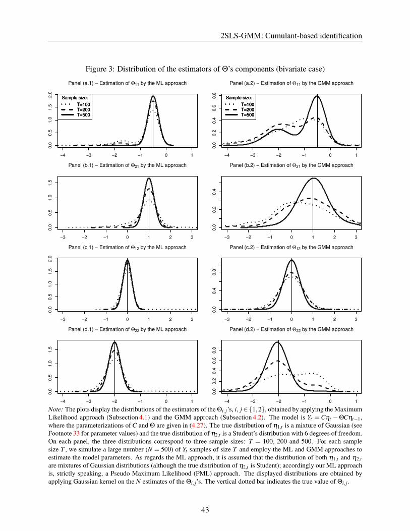
2SLS-GMM: Cumulant-based identification
Figure 3: Distribution of the estimators of Θ’s components (bivariate case)
−4 −3 −2 −1 0 1
0.0
0.5
1.0
1.5
2.0
Panel (a.1) − Estimation of Θ11 by the ML approach
Sample size:
T=100T=200T=500
Sample size:
T=100T=200T=500
Sample size:
T=100T=200T=500
−4 −3 −2 −1 0 1
0.0
0.2
0.4
0.6
0.8
Panel (a.2) − Estimation of Θ11 by the GMM approach
Sample size:
T=100T=200T=500
Sample size:
T=100T=200T=500
Sample size:
T=100T=200T=500
−3 −2 −1 0 1 2 3
0.0
0.5
1.0
1.5
Panel (b.1) − Estimation of Θ21 by the ML approach
−3 −2 −1 0 1 2 3
0.0
0.2
0.4
Panel (b.2) − Estimation of Θ21 by the GMM approach
−3 −2 −1 0 1 2 3
0.0
0.5
1.0
1.5
2.0
Panel (c.1) − Estimation of Θ12 by the ML approach
−3 −2 −1 0 1 2 3
0.0
0.4
0.8
Panel (c.2) − Estimation of Θ12 by the GMM approach
−4 −3 −2 −1 0 1
0.0
0.5
1.0
1.5
Panel (d.1) − Estimation of Θ22 by the ML approach
−4 −3 −2 −1 0 1
0.0
0.2
0.4
0.6
0.8
Panel (d.2) − Estimation of Θ22 by the GMM approach
Note: The plots display the distributions of the estimators of the Θi, j’s, i, j∈{1,2}, obtained by applying the MaximumLikelihood approach (Subsection 4.1) and the GMM approach (Subsection 4.2). The model is Yt = Cηt −ΘCηt−1,where the parameterizations of C and Θ are given in (4.27). The true distribution of η1,t is a mixture of Gaussian (seeFootnote 33 for parameter values) and the true distribution of η2,t is a Student’s distribution with 6 degrees of freedom.On each panel, the three distributions correspond to three sample sizes: T = 100, 200 and 500. For each samplesize T , we simulate a large number (N = 500) of Yt samples of size T and employ the ML and GMM approaches toestimate the model parameters. As regards the ML approach, it is assumed that the distribution of both η1,t and η2,tare mixtures of Gaussian distributions (although the true distribution of η2,t is Student); accordingly our ML approachis, strictly speaking, a Pseudo Maximum Likelihood (PML) approach. The displayed distributions are obtained byapplying Gaussian kernel on the N estimates of the Θi, j’s. The vertical dotted bar indicates the true value of Θi, j.
43
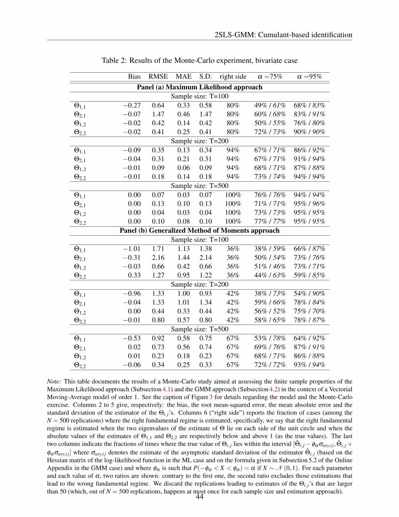
2SLS-GMM: Cumulant-based identification
Table 2: Results of the Monte-Carlo experiment, bivariate case
Bias RMSE MAE S.D. right side α =75% α =95%Panel (a) Maximum Likelihood approach
Sample size: T=100Θ1,1 −0.27 0.64 0.33 0.58 80% 49% / 61% 68% / 83%Θ2,1 −0.07 1.47 0.46 1.47 80% 60% / 68% 83% / 91%Θ1,2 −0.02 0.42 0.14 0.42 80% 50% / 55% 76% / 80%Θ2,2 −0.02 0.41 0.25 0.41 80% 72% / 73% 90% / 90%
Sample size: T=200Θ1,1 −0.09 0.35 0.13 0.34 94% 67% / 71% 86% / 92%Θ2,1 −0.04 0.31 0.21 0.31 94% 67% / 71% 91% / 94%Θ1,2 −0.01 0.09 0.06 0.09 94% 68% / 71% 87% / 88%Θ2,2 −0.01 0.18 0.14 0.18 94% 73% / 74% 94% / 94%
Sample size: T=500Θ1,1 0.00 0.07 0.03 0.07 100% 76% / 76% 94% / 94%Θ2,1 0.00 0.13 0.10 0.13 100% 71% / 71% 95% / 96%Θ1,2 0.00 0.04 0.03 0.04 100% 73% / 73% 95% / 95%Θ2,2 0.00 0.10 0.08 0.10 100% 77% / 77% 95% / 95%
Panel (b) Generalized Method of Moments approachSample size: T=100
Θ1,1 −1.01 1.71 1.13 1.38 36% 38% / 59% 66% / 87%Θ2,1 −0.31 2.16 1.44 2.14 36% 50% / 54% 73% / 76%Θ1,2 −0.03 0.66 0.42 0.66 36% 51% / 46% 73% / 71%Θ2,2 0.33 1.27 0.95 1.22 36% 44% / 63% 59% / 85%
Sample size: T=200Θ1,1 −0.96 1.33 1.00 0.93 42% 38% / 73% 54% / 90%Θ2,1 −0.04 1.33 1.01 1.34 42% 59% / 66% 78% / 84%Θ1,2 0.00 0.44 0.33 0.44 42% 56% / 52% 75% / 70%Θ2,2 −0.01 0.80 0.57 0.80 42% 58% / 65% 78% / 87%
Sample size: T=500Θ1,1 −0.53 0.92 0.58 0.75 67% 53% / 78% 64% / 92%Θ2,1 0.02 0.73 0.56 0.74 67% 69% / 76% 87% / 91%Θ1,2 0.01 0.23 0.18 0.23 67% 68% / 71% 86% / 88%Θ2,2 −0.06 0.34 0.25 0.33 67% 72% / 72% 93% / 94%
Note: This table documents the results of a Monte-Carlo study aimed at assessing the finite sample properties of theMaximum Likelihood approach (Subsection 4.1) and the GMM approach (Subsection 4.2) in the context of a VectorialMoving-Average model of order 1. See the caption of Figure 3 for details regarding the model and the Monte-Carloexercise. Columns 2 to 5 give, respectively: the bias, the root mean-squared error, the mean absolute error and thestandard deviation of the estimator of the Θi, j’s. Columns 6 (“right side”) reports the fraction of cases (among theN = 500 replications) where the right fundamental regime is estimated; specifically, we say that the right fundamentalregime is estimated when the two eigenvalues of the estimate of Θ lie on each side of the unit circle and when theabsolute values of the estimates of Θ1,1 and Θ2,2 are respectively below and above 1 (as the true values). The lasttwo columns indicate the fractions of times where the true value of Θi, j lies within the interval [Θi, j−φα σasy,i j,Θi, j +
φα σasy,i j] where σasy,i j denotes the estimate of the asymptotic standard deviation of the estimator Θi, j (based on theHessian matrix of the log-likelihood function in the ML case and on the formula given in Subsection 5.2 of the OnlineAppendix in the GMM case) and where φα is such that P(−φα < X < φα) = α if X ∼N (0,1). For each parameterand each value of α , two ratios are shown: contrary to the first one, the second ratio excludes those estimations thatlead to the wrong fundamental regime. We discard the replications leading to estimates of the Θi, j’s that are largerthan 50 (which, out of N = 500 replications, happens at most once for each sample size and estimation approach).
44

2SLS-GMM: Cumulant-based identification
Table 3: Estimated SVARMA models (GNP and Unemployment rate)
Approach: GMM MLparam. std dev. param. std dev.
Φ1,[1,1] 0.883 (0.540) 0.641 (0.199)Φ1,[2,1] −0.425 (0.355) −0.229 (0.096)Φ1,[1,2] 0.064 (1.323) −0.832 (0.367)Φ1,[2,2] 1.153 (0.722) 1.744 (0.193)Φ2,[1,1] 0.210 (0.166) 0.233 (0.082)Φ2,[2,1] −0.069 (0.088) −0.029 (0.038)Φ2,[1,2] 1.187 (1.661) 2.039 (0.511)Φ2,[2,2] −0.565 (0.904) −1.271 (0.246)Φ3,[1,1] −0.165 (0.172) −0.332 (0.077)Φ3,[2,1] 0.019 (0.091) 0.035 (0.038)Φ3,[1,2] −1.763 (0.995) −1.467 (0.434)Φ3,[2,2] 0.600 (0.688) 0.609 (0.208)Φ4,[1,1] 0.048 (0.107) 0.164 (0.059)Φ4,[2,1] 0.016 (0.072) −0.012 (0.031)Φ4,[1,2] 0.604 (0.490) 0.321 (0.182)Φ4,[2,2] −0.198 (0.320) −0.101 (0.098)Θ1,1 0.814 (0.328) 0.388 (0.191)Θ2,1 −0.468 (0.126) 0.005 (0.096)Θ1,2 −2.733 (0.858) −2.048 (0.305)Θ2,2 1.496 (0.393) 1.775 (0.148)C1,1 0.298 (0.092) 0.555 (0.044)C2,1 0.172 (0.028) −0.195 (0.017)C1,2 0.689 (0.082) 0.645 (0.059)C2,2 0.007 (0.072) −0.006 (0.017)κ3,1 3.136 (0.126) µ1,1 0.421 (0.209)κ3,2 0.071 (0.328) µ2,1 −0.130 (0.020)κ4,1 19.828 (0.393) σ1,1 1.242 (0.099)κ4,2 1.459 (0.858) σ2,1 0.081 (0.012)
p1 0.448 (0.115)p2 0.286 (0.040)
Note: This table reports the results of the estimation of bivariate VARMA(4,1) models. The dataset is the one usedin Blanchard and Quah (1989); it covers the period from 1948Q1 to 1987Q4 at the quarterly frequency. The firstendogenous variable is the U.S. real GNP growth (i.e. ∆gnp, where gnp = log(GNP)) and the second endogenousvariable is the unemployment rate. The model is: Φ(L)Yt = (I−ΘL)Cηt , where, for j ∈ {1,2}, η j,t is drawn fromN (µ j,1σ2
j,1) with probability p j and from N (µ j,2σ2j,2) with probability 1− p j. We impose E(η j,t) = 0 and V (η j,t) =
1, which implies that µ j,2 and σ j,2 can be deduced from µ j,1, σ j,1 and p j. Both the Maximum Likelihood (ML) and the2SLS-GMM approaches are employed to estimate the model (see Subsections 4.1 and 4.2, respectively). Asymptoticstandard deviations are reported in parentheses. Φk,[i, j] is the (i, j) element of Φk, with Φ(L) = I−Φ1L−·· ·−ΦpLp.
45

2SLS-GMM: Cumulant-based identification
Figure 4: Estimated shock distributions
−4 −2 0 2 4
0.0
0.1
0.2
0.3
0.4
0.5
0.6
0.7
Distribution of η1
Kernel density estimate
Estimated parametric distribution (Gaussian mixture)
Standardized normal distribution N(0,1)
−3 −2 −1 0 1 2 3
0.0
0.5
1.0
1.5
2.0
Distribution of η2
Note: This figure displays the estimated p.d.f. of the structural shocks η j,t , for j ∈ {1,2} resulting from the MLestimation of a SVARMA(4,1) model using Blanchard and Quah (1989)’s dataset. The dotted lines correspond to theestimated parametric distributions (mixture of Gaussian distributions): η j,t is drawn from N (µ j,1σ2
j,1) with proba-bility p j and from N (µ j,2σ2
j,2) with probability 1− p j; µ j,2 and σ j,2 are computed so as to have E(η j,t) = 0 andV (η j,t) = 1. The model parameterization is detailed in the caption of Table 3. The black solid lines correspond tokernel-based density estimates of the distribution of the (estimated) structural shocks η j,t . The latter are computedby applying the backward/forward filtering algorithm underlying function at (see Subsection 4.1.2 for details on thisalgorithm). For the sake of comparison, we also report the N (0,1) p.d.f. (dashed lines).
46

2SLS-GMM: Cumulant-based identification
Figure 5: IRFs – GNP and unemployment rate
0 10 20 30 40
−0
.50
.00
.51
.01
.52
.0
Responses of GNP to Shock 1
BQ Method
ML Method
0 10 20 30 40
−0
.50
.00
.51
.01
.52
.0
Responses of GNP to Shock 2
0 10 20 30 40
−0
.8−
0.4
0.0
0.2
0.4
Responses of unemployment rate to Shock 1
0 10 20 30 40
−0
.8−
0.4
0.0
0.2
0.4
Responses of unemployment rate to Shock 2
Note: This figure compares impulse response functions (IRFs) associated with models resulting from the BQ approach(long-run restrictions à la Blanchard and Quah, 1989, 8-lag VAR model) as well as the Maximum Likelihood (ML)approach (Subsection 4.1, VARMA(4,1) model). The dataset is the same as in Blanchard and Quah (1989). In thecontext of the BQ approach, whereas Shock 1 (first column of plots) is interpreted as a demand shock, Shock 2(second column of plots) is interpreted as a supply shock. In BQ, by construction, the long-run impact of the demandshock (Shock 1) on real GNP is null. In the ML approach, Shock 1 is defined as the shock having the lower influenceon the long-run GNP variance. For the GNP variable, we report the cumulated impacts of the shocks on the (log) GNPgrowth rate.
47

2SLS-GMM: Cumulant-based identification
Figure 6: Nonfundamentalness regimes when n = 2
I IIIV
III
V
−1
+1
Tr(Θ)
det(Θ)
Note: This figure shows the 5 regions corresponding to the different (non)fundamentalness regimes when Yt is ofdimension 2 (i.e. when Θ is of dimension 2× 2). Region I is purely fundamental; Regions III and V are purelynonfundamental; Regions II and IV are mixed. The dashed line represents the pairs (Tr(Θ),det(Θ)) for which thediscriminant Tr(Θ)2− 4det(Θ) is zero; the area that is below (respectively above) this parabola corresponds to real(resp. complex) eigenvalues for Θ.
48

REFERENCES
ReferencesAkaike, H., 1974, “A New Look at the Statistical Model Identification,” IEEE Transactions on Automatic
Control, 19(6), 716–723.Alessi, L., M. Barigozzi, and M. Capasso, 2011, “Non-Fundamentalness in Structural Econometric Models:
A Review,” International Statistical Review, 79(1), 16–47.Bai, J., and S. Ng, 2005, “Tests for Skewness, Kurtosis, and Normality for Time Series Data,” Journal of
Business & Economic Statistics, 23, 49–60.Barsky, R. B., and E. R. Sims, 2012, “Information, Animal Spirits, and the Meaning of Innovations in
Consumer Confidence,” American Economic Review, 102(4), 1343–1377.Bates, C., and H. White, 1985, “A Unified Theory of Consistent Estimation for Parametric Models,” Econo-
metric Theory, 1(02), 151–178.Beaudry, P., P. Fève, A. Guay, and F. Portier, 2015, “When is Nonfundamentalness in VARs a Real Problem?
An Application to News Shocks,” NBER Working Papers 21466, National Bureau of Economic Research.Bernanke, B. S., 1986, “Alternative Explanations of the Money-Income Correlation,” Carnegie-Rochester
Conference Series on Public Policy, 25(1), 49–99.Blanchard, O. J., J.-P. L’Huillier, and G. Lorenzoni, 2013, “News, Noise, and Fluctuations: An Empirical
Exploration,” American Economic Review, 103(7), 3045–3070.Blanchard, O. J., and D. Quah, 1989, “The Dynamic Effects of Aggregate Demand and Supply Distur-
bances,” American Economic Review, 79(4), 655–73.Bonhomme, S., and J.-M. Robin, 2009, “Consistent Noisy Independent Component Analysis,” Journal of
Econometrics, 149(1), 12–25.Boudt, K., D. Cornilly, and T. Verdonck, 2018, “Nearest Comoment Estimation with Unobserved Factors,”
working paper.Box, G. E. P., and G. Jenkins, 1970, Time Series Analysis, Forecasting and Control. Holden-Day, San
Francisco.Box, G. E. P., and D. A. Pierce, 1970, “Distribution of Residual Autocorrelations in Autoregressive-
Integrated Moving Average Time Series Models,” Journal of the American Statistical Association,65(332), 1509–1526.
Breidt, F. J., and R. A. Davis, 1992, “Time-Reversibility, Identifiability and Independence of Innovationsfor Stationary Time Series,” Journal of Time Series Analysis, 13(5), 377–390.
Brockwell, P. J., and R. A. Davis, 1991, Time Series: Theory and Methods. 2nd ed., Springer-Verlag NewYork., New York, NY, USA.
Chahrour, R., and K. Jurado, 2018, “News or Noise? The Missing Link,” American Economic Review,108(7), 1702–1736.
Chan, K.-S., and L.-H. Ho, 2004, “On the Unique Representation of non-Gaussian Multivariate LinearProcesses,” Working papers, Department of Statistics & Actuarial Science, University of Iowa.
Chan, K.-S., L.-H. Ho, and H. Tong, 2006, “A Note on Time-Reversibility of Multivariate Linear Processes,”Biometrika, 93(1), 221–227.
Chari, V., P. J. Kehoe, and E. R. McGrattan, 2008, “Are Structural VARs with Long-run Restrictions Usefulin Developing Business Cycle Theory?,” Journal of Monetary Economics, 55(8), 1337–1352.
Chen, B., J. Choi, and J. C. Escanciano, 2017, “Testing for Fundamental Vector Moving Average Represen-tations,” Quantitative Economics, 8(1), 149–180.
Chen, M.-C., R. A. Davis, and L. Song, 2011, “Inference for Regression Models with Errors from a Non-invertible MA(1) Process,” Journal of Forecasting, 30(1), 6–30.
Cheng, Q., 1992, “On The Unique Representation of Non-Gaussian Linear Processes,” The Annals of Statis-tics, 20, 1143–1145.
49

REFERENCES
Christiano, L. J., M. Eichenbaum, and R. Vigfusson, 2006, “Alternative Procedures for Estimating VectorAutoregressions Identified with Long-Run Restrictions,” Journal of the European Economic Association,4(2-3), 475–483.
, 2007, “Assessing Structural VARs,” in NBER Macroeconomics Annual. MIT Press, Cambridge,pp. 1–106.
Cochrane, J. H., 1994, “Shocks,” Carnegie-Rochester Conference Series on Public Policy, 41, 295–364.Comon, P., 1994, “Independent Component Analysis, A New Concept?,” Signal Processing, 36, 287–314.Darmois, G., 1953, “Analyse Générale des Liaisons Stochastiques: Etude Particulière de l’Analyse Facto-
rielle Linéaire,” Revue de l’Institut International de Statistique, 21(1/2), 2–8.Deistler, M., and J. Schrader, 1979, “Linear Models with Autocorrelated Errors: Identifiability without
Minimality Assumptions,” Econometrica, 47, 495–504.Economic Sciences Prize Committee, 2011, “Thomas J. Sargent and Christopher A. Sims: Empirical
Macroeconomics,” Nobel Prize in Economics documents 2011-2, Nobel Prize Committee.Engle, R. F., and C. W. J. Granger, 1987, “Co-integration and Error Correction: Representation, Estimation,
and Testing,” Econometrica, 55(2), 251–276.Erceg, C., G. L., and C. Gust, 2005, “Can Long Run Restriction Identify Technology Shocks?,” Journal of
the European Economic Association, 3, 1237–1278.Eriksson, J., and V. Koivunen, 2004, “Identifiability, Separability and Uniqueness of Linear ICA Models,”
IEEE Signal Processing Letters, 11, 601–604.Evans, C., and D. Marshall, 2011, “Fundamental Economic Shocks and the Macroeconomy,” Discussion
Paper 351, Central Bank of Chile.Faust, J., and E. Leeper, 1997, “When Do Long Run Identifying Restrictions Give Reliable Results?,”
Journal of Business and Economic Statistics, 15, 345–353.Fernandez-Villaverde, J., J. Rubio-Ramirez, T. Sargent, and M. Watson, 2007, “A,B,C’s (and D)’s for Un-
derstanding VAR’s,” American Economic Review, 97, 1021–1026.Fève, P., J. Matheron, and J.-G. Sahuc, 2009, “On the Dynamic Implications of News Shocks,” Economics
Letters, 102, 96–98.Findley, D., 1986, “The Uniqueness of Moving Average Representation with Independent and Identically
Distributed Random Variables for Non-Gaussian Stationary Time Series,” Biometrika, 73, 520–521.Forni, M., and L. Gambetti, 2014, “Sufficient Information in Structural VARs,” Journal of Monetary Eco-
nomics, 66(C), 124–136.Forni, M., L. Gambetti, M. Lippi, and L. Sala, 2017a, “Noise Bubbles,” Economic Journal, 127(604), 1940–
1976., 2017b, “Noisy News in Business Cycles,” American Economic Journal: Macroeconomics, 9(4),
122–152.Francis, N., and V. Ramey, 2005, “Is Technology-Driven Real Business Cycle Hypothesis Dead? Shocks
and Aggregate Fluctuations Revisited,” Journal of Monetary Economics, 52, 1379–1399.Gagliardini, P., and C. Gouriéroux, 2018, “Identification by Laplace Transforms in Nonlinear Panel or Time
Series Models with Unobserved Stochastic Dynamic Effects,” Journal of Econometrics, forthcoming.Galbraith, J., A. Ullah, and V. Zinde-Walsh, 2002, “Estimation of the Vector Moving Average Model by
Vector Autoregression,” Econometric Reviews, 21(2), 205–219.Gali, J., and P. Rabanal, 2005, “Technology Shocks and Aggregate Fluctuations: How Well Does the RBC
Model Fit Postwar US Data?,” in NBER Macroeconomics Annual. MIT Press, Cambridge, vol. 19.Ghurye, S., and I. Olkin, 1961, “A Characterization of the Multivariate Normal Distribution,” Annals of
Mathematical Statistics, 33, 533–541.Giannone, D., and L. Reichlin, 2006, “Does Information Help Recovering Structural Shocks From Past
Observations?,” Journal of European Economic Association, 4, 455–465.
50

REFERENCES
Gospodinov, N., and S. Ng, 2015, “Minimum Distance Estimation of Possibly Noninvertible MA Process,”Journal of Business and Economic Statistics, 33, 403–417.
Gouriéroux, C., and J. Jasiak, 2016, “Filtering and Prediction in Noncausal Processes,” Journal of TimeSeries Analysis, 37, 405–430.
Gouriéroux, C., A. Monfort, and E. Renault, 1989, “Testing for Common Roots,” Econometrica, 57, 171–185.
Gouriéroux, C., A. Monfort, and J.-P. Renne, 2017, “Statistical Inference for Independent Component Anal-ysis,” Journal of Econometrics, 196, 111–126.
Gouriéroux, C., and J.-M. Zakoian, 2015, “On Uniqueness of Moving Average Representation of HeavyTailed Stationary Processes,” Journal of Time Series Analysis, 36, 876–887.
Grassi, S., F. Ferroni, and M. Leon-Ledesma, 2015, “Fundamental Shock Selection in DSGE Models,”working paper.
Guay, A., and M. Normandin, 2018, “Identification of Structural Vector Autoregressions Through HigherUnconditional Moments,” Working paper, UQAM and HEC Montreal.
Hannan, E., and M. Deistler, 1996, The Statistical Theory of Linear Systems. Wiley, New York edn.Hannan, E. J., and B. G. Quinn, 1979, “The Determination of the Order of an Autoregression,” Journal of
the Royal Statistical Society, 41(2), 190–195.Hansen, L., and R. Hodrick, 1980, “Forward Exchange Rates as Optimal Predictors of Future Sport Rates:
An Econometric Analysis,” Journal of Political Economy, 88, 829–853.Hansen, L., and T. Sargent, 1980, “Formulating and Estimating Dynamic Linear Rational Expectations
Models,” Journal of Economic Dynamics and Control, 2, 7–46., 1991, “Two Difficulties in Interpreting Vector Autoregressions,” in Rational Expectations Econo-
metrics. L., Hansen and T., Sargent, editors, Westview Press, Boulder, vol. 19.Herwartz, H., and H. Lütkepohl, 2017, “Structural Vector Autoregressions with Markov Switching: Com-
bining Conventional with Statistical Identification of Shocks,” Journal of Econometrics, forthcoming.Hyvärinen, A., J. Karhunen, and E. Oja, 2001, Independent Component Analysis. Wiley, New York edn.Jennrich, R., 1969, “Asymptotic Properties of Nonlinear Least Squares Estimation,” The Annals of Mathe-
matical Statistics, 40, 633–643.Koop, G., M. H. Pesaran, and S. M. Potter, 1996, “Impulse Response Analysis in Nonlinear Multivariate
Models,” Journal of Econometrics, 74(1), 119–147.Kydland, F., and E. Prescott, 1982, “Time to Build and Aggregate Fluctuations,” Econometrica, 50, 1345–
1370.Lanne, M., H. Lütkepohl, and K. Maciejowska, 2010, “Structural Vector Autoregressions with Markov
Switching,” Journal of Economic Dynamics and Control, 34, 121–131.Lanne, M., M. Meitz, and P. Saikkonen, 2017, “Identification and Estimation of Non-Gaussian Structural
Vector Autoregressions,” Journal of Econometrics, 196(2), 288–304.Leeper, E., T. Walker, and S. Yang, 2013, “Fiscal Foresight and Information Flows,” Econometrica, 81,
1115–1145.Lii, K.-S., and M. Rosenblatt, 1992, “An Approximate Maximum Likelihood Estimation for Non-Gaussian
Non-minimum Phase Moving Average Processes,” Journal of Multivariate Analysis, 43, 272–299., 1996, “Maximum Likelihood Estimation for Non-Gaussian Nonminimum Phase ARMA Se-
quences,” Statistica Sinica, 6, 1–22.Lippi, M., and L. Reichlin, 1993, “The Dynamic Effects of Aggregate Demand and Supply Disturbances:
Comment,” American Economic Review, 83, 644–652., 1994, “VAR Analysis, Nonfundamental Representations, Blaschke Matrices,” Journal of Econo-
metrics, 63, 307–325.Ljung, G. M., and G. E. P. Box, 1978, “On a Measure of Lack of Fit in Time Series Models,” Biometrika,
51

REFERENCES
65(2), 297–303.Lobato, I. N., and C. Velasco, 2004, “A Simple Test of Normality for Time Series,” Econometric Theory,
20(4), 671–689., 2018, “Frequency Domain Minimum Distance Inference for Possibly Noninvertible and Noncausal
ARMA Models,” Annals of Statistics, 46(2), 555–579.Lof, M., 2013, “Noncausality and Asset Pricing,” Studies in Nonlinear Dynamics and Econometrics, 17,
211–220.Lorenzoni, G., 2009, “A Theory of Demand Shocks,” American Economic Review, 99(5), 2050–2084.Lütkepohl, H., 2013, “Identifying Structural Vector Autoregression via Changes in Volatility,” in VAR Mod-
els in Macroeconomics, Essays in Honor of Christopher Sims, Advances in Econometrics. Thomas B.Fomby , Lutz Kilian , Anthony Murphy, editors, Emerald Group Publishing Limited, vol. 32.
, 2014, “Fundamental Problems with Nonfundamental Shocks,” in Essays in Nonlinear Time SeriesEconometrics. N., Haldrup, M., Meltz and P., Saikkonen, editors, Oxford University Press.
Lütkepohl, H., and B. Theilen, 1991, “Measures of Multivariate Skewness and Kurtosis for Tests of Non-normality,” Statistical Papers, 32(1), 179–193.
Mertens, K., and M. Ravn, 2010, “Measuring the Impact of Fiscal Policy in the Face of Anticipation: AStructural VAR Approach,” Economic Journal, 120(544), 393–413.
Mountford, A., and H. Uhlig, 2009, “What Are the Effects of Fiscal Policy Shocks?,” Journal of AppliedEconometrics, 24, 960–992.
Pesaran, H. H., and Y. Shin, 1998, “Generalized Impulse Response Analysis in Linear Multivariate Models,”Economics Letters, 58(1), 17–29.
Rosenblatt, M., 2000, Gaussian and Non Gaussian Linear Time Series and Random Fields. Springer Verlag,New York edn.
Rozanov, Y., 1960, “Spectral Properties of Multivariate Stationary Processes and Boundary Properties ofAnalytic Matrices,” Theory of Probability and its Applications, 5, 362–376.
, 1967, Stationary Random Processes. Holden Day edn.Rubio-Ramirez, J., D. Waggoner, and T. Zha, 2010, “Structural Vector Autoregression: Theory of Identifi-
cation and Algorithms for Inference,” Review of Economic Studies, 77, 665–696.Schwarz, G., 1978, “Estimating the Dimension of a Model,” The Annals of Statistics, 6(2), 461–464.Shapiro, S. S., and M. B. Wilk, 1965, “An Analysis of Variance Test for Normality (Complete Samples),”
Biometrika, 52(3-4), 591–611.Sims, C., 1980, “Macroeconomics and Reality,” Econometrica, 48, 1–48.
, 1986, “Are Forecasting Models Usable for Policy Analysis?,” Federal Reserve Bank of Minneapo-lis Quarterly Review, 10, 1–16.
, 1989, “Models and their Uses,” American Journal of Agricultural Economics, 71, 489–494.Sims, E. R., 2012, “News, Non-Invertibility, and Structural VARs,” Working Papers 013, University of Notre
Dame, Department of Economics.Skitovich, V., 1953, “On a Property of a Normal Distribution,” Doklady Academii nauk SSSR, (in Russian),
89, 217–219.Smets, F., and R. Wouters, 2003, “An Estimated Dynamic Stochastic General Equilibrium Model of the
Euro Area,” Journal of the European Economic Association, 1, 1123–1175.Söderlind, P., 1999, “Solution and Estimation of RE Macromodels with Optimal Policy,” European Eco-
nomic Review, 43(4-6), 813–823.Uhlig, H., 2005, “What Are the Effects of Monetary Policy on Output? Results From an Agnostic Identifi-
cation Procedure,” Journal of Monetary Economics, 52, 381–419.Velinov, A., and W. Chen, 2014, “Are There Bubbles in Stock Prices? Testing for Fundamental Shocks,”
Dp diw berlin, DIW.
52

REFERENCES
Wald, A., 1949, “Note on the Consistency of the Maximum Likelihood Estimate,” The Annals of Mathemat-ical Statistics, 20(4), 595–601.
Weiss, G., 1975, “Time-Reversibility of Linear Stochastic Processes,” Journal of Applied Probability, 12(4),831–836.
Wu, R., and R. A. Davis, 2010, “Least Absolute Deviation Estimation for General Autoregressive MovingAverage Time-Series Models,” Journal of Time Series Analysis, 31(2), 98–112.
53