identifying protein complexes in high-throughput …

September 23, 2005 18:49 Proceedings Trim Size: 9in x 6in chu

IDENTIFYING PROTEIN COMPLEXES INHIGH-THROUGHPUT PROTEIN INTERACTION SCREENS

USING AN INFINITE LATENT FEATURE MODEL∗

WEI CHU & ZOUBIN GHAHRAMANI

Gatsby Computational Neuroscience Unit,University College London,London, WC1N 3AR, UK

E-mail: chuwei,[email protected]

ROLAND KRAUSE

Max-Planck-Institute for Molecular GeneticsD-10117 Berlin, Germany

E-mail: [email protected]

DAVID L. WILD

Keck Graduate Institute of Applied Life SciencesClaremont, CA 91171, USA

E-mail: [email protected]

We propose a Bayesian approach to identify protein complexes and their con-stituents from high-throughput protein-protein interaction screens. An infinitelatent feature model that allows for multi-complex membership by individual pro-teins is coupled with a graph diffusion kernel that evaluates the likelihood of twoproteins belonging to the same complex. Gibbs sampling is then used to infer acatalog of protein complexes from the interaction screen data. An advantage ofthis model is that it places no prior constraints on the number of complexes andautomatically infers the number of significant complexes from the data. Validationresults using affinity purification/mass spectrometry experimental data from yeastRNA-processing complexes indicate that our method is capable of partitioning thedata in a biologically meaningful way.A supplementary web site containing larger versions of the figures is available athttp://public.kgi.edu/∼wild/PSB06/index.html.

∗This work was supported by the National Institutes of Health Grant Number 1 P01GM63208. A part of this work was carried out at Institute for Pure and Applied Math-ematics (IPAM) of UCLA. We are grateful to Thomas L. Griffiths for the Matlab scriptof the Gibbs sampler.

Pacific Symposium on Biocomputing 11:231-242(2006)


1. Introduction

The analysis of protein-protein interactions forms an essential part of the“systems biology” enterprise. Many cellular functions are performed bymulti-protein complexes and the identification and analysis of protein com-plex membership reveals insights into both the topological properties andfunctional organization of protein networks. Recently, high-throughputtechniques have been developed to investigate physical binding betweenthe constituents of protein complexes on a proteome-wide scale. The yeasttwo-hybrid assay (Y2H), a means of assessing whether two single proteinsinteract, has been adapted to systematically test pairwise protein interac-tions on a large scale1,2, whereas affinity purification techniques using massspectrometry (APMS)3 provide a particularly effective approach to iden-tifying protein complexes that contain more than two components. Thesetechniques have been used to perform large scale protein-protein interac-tion screens in the yeast Saccharomyces cerevisiae4,5,6 and the bacteriumEscherichia coli7.

In the APMS techniques, as described by Kumar and Snyder3, individ-ual proteins are tagged and used as “baits” to form physiological complexeswith other proteins in the cells. Then, using the tag, each bait protein ispurified, retrieving the proteins to which it binds, which may sometimesconstitute the entire complex. The proteins extracted with the bait proteinare identified using standard mass spectrometry methods. The raw resultsof these experiments are often referred to as “purifications” and may differsubstantially from what is thought to exist in the cell and what is anno-tated in databases of protein complexes. Identification of actual proteincomplexes from these “purifications” often involves manual post-processingbased on the existence of overlaps between the purifications4. Attempts toautomate complex identification have involved the use of binary protein-protein interaction graphs8,9,10, unsupervised clustering based on specialsimilarity measures13,6 and graph-theoretic approaches14. However, theseapproaches are bedeviled by a number of problems, such as fact that theexact number of complexes is initially unknown; the presence of poten-tial contaminant proteins (which may themselves form complexes); the factthat the experiments do not always retrieve whole complexes, but onlysub-complexes; and the presence of shared components, which need to beassigned to more than one complex.

In this paper, we propose a probabilistic algorithm to identify proteincomplex membership using the data from affinity purification/mass spec-



a

1 2 2 2 1 1 11 2 2 2 1 1 1

a b c d e f g1 1 1 1 0 0 0

bc

(iii) Adjacency Matrix, A

d 1 2 2 3 2 2 2

0 1 1 2 2 2 20 1 1 2 2 2 20 1 1 2 2 2 2

efg

d

cb

e

a

de

gf Bait a

0 0 0 1 1 1 10 1 1 1 1 1 1

a b c d e f g1 1 1 1 0 0 0

Bait dBait f

Protein

(i) Native Protein Complexes (ii) Purification Matrix, B

(iv) Complex Membership, Z

a b c d e f g

1 1 1 1 1 0 01

2 0 0 0 1 1 1 1... ...

3

... ...

... ...

... ...

... ...

... ...

... ...

... ...

0 0 0 0 0 0 0

Complex

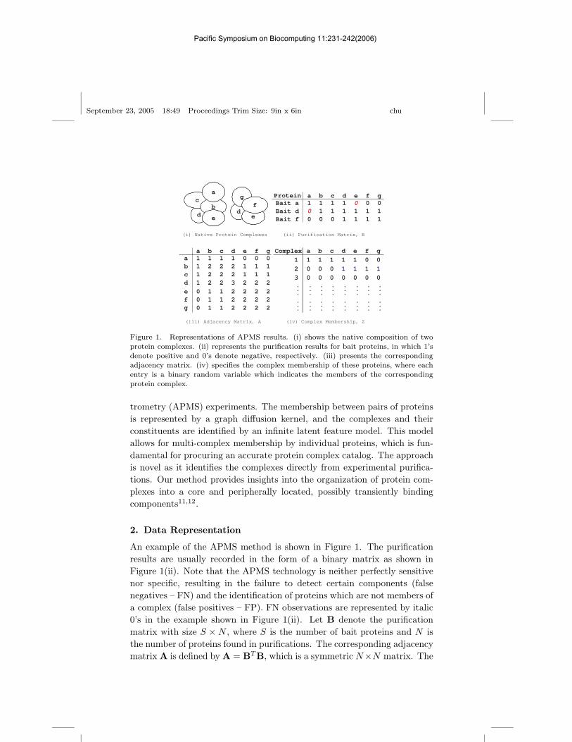
Figure 1. Representations of APMS results. (i) shows the native composition of twoprotein complexes. (ii) represents the purification results for bait proteins, in which 1’sdenote positive and 0’s denote negative, respectively. (iii) presents the correspondingadjacency matrix. (iv) specifies the complex membership of these proteins, where eachentry is a binary random variable which indicates the members of the correspondingprotein complex.

trometry (APMS) experiments. The membership between pairs of proteinsis represented by a graph diffusion kernel, and the complexes and theirconstituents are identified by an infinite latent feature model. This modelallows for multi-complex membership by individual proteins, which is fun-damental for procuring an accurate protein complex catalog. The approachis novel as it identifies the complexes directly from experimental purifica-tions. Our method provides insights into the organization of protein com-plexes into a core and peripherally located, possibly transiently bindingcomponents11,12.

2. Data Representation

An example of the APMS method is shown in Figure 1. The purificationresults are usually recorded in the form of a binary matrix as shown inFigure 1(ii). Note that the APMS technology is neither perfectly sensitivenor specific, resulting in the failure to detect certain components (falsenegatives – FN) and the identification of proteins which are not members ofa complex (false positives – FP). FN observations are represented by italic0’s in the example shown in Figure 1(ii). Let B denote the purificationmatrix with size S × N , where S is the number of bait proteins and N isthe number of proteins found in purifications. The corresponding adjacencymatrix A is defined by A = BT B, which is a symmetric N×N matrix. The



ij-th element, Aij , is the number of purifications in which both protein i

and protein j appear. The similarity between protein pairs can be measuredby a graph diffusion kernel15 based on A. In this work, we focus on thevon Neumann diffusion kernel16 as the closeness measure. Kernel methodshave also been applied to the inference of biological networks from otherdata sources17,18.

3. The von Neumann Diffusion Kernel

The element Aij in the adjacency matrix can be thought of as the numberof distinct “paths” between protein i and protein j discovered by the APMSexperiment. For example in Figure 1, there are two paths between proteind and protein e and no path directly connecting protein a and protein e.However, we could also reach protein e indirectly from protein a via thepaths through the neighbors of protein a, e.g. a-b-e a-c-e and a-d-e. Thenumber of distinct paths with length 2 between a pair of proteins can bedirectly counted by the matrix product AA. More generally, the numberof paths from protein i to protein j of length � on the graph can be directlycounted as the ij-th element of the matrix A�. The closeness between a pairof proteins can be measured by the number of distinct paths with differentlength. The von Neumann diffusion kernel16 is the limit of the sum of thegeometric series, defined as

K :=∞∑

�=1

γ�−1A� = A (1 − γA)−1. (1)

where γ is the diffusion factor to ensure the longer range connections de-cay exponentially.a The normalized kernel is an appropriate measure ofsimilarity, which is defined as

Dij =Kij√KiiKjj

. (2)

Note that the matrix elements are between 0 and 1. Dij = 0 implies proteini is isolated from protein j. On the contrary, Dij approaches 1 if the proteinpair is tightly connected. The elements of the normalized von Neumannkernel (2) provide a probabilistic measure on the pairwise membership oftwo proteins in the same complex. This interpretation makes Dij suitablefor use as a likelihood in a probabilistic model, which we now describe.

aThe von Neumann kernel (1) is positive definite only if 0 < γ < ρ−1 where ρ is

the spectral radius of A. γ could be learnt from the data. In this work, we set γ =(1+κ)−1ρ−1 where κ is the proportion of non-zero elements in the adjacency matrix A.



4. Protein Complex Membership

Protein complex membership can be represented as a binary matrix, de-noted as Z (see Figure 1(iv)). Each column of the matrix Z is denoted byzi, known as the feature vector of the protein. The length of zi is variable,as the number of protein complexes is actually unknown. The membershipof the i-th protein in complex c is indicated by a binary random variablezci. Note that each protein may belong to multiple complexes. The learn-ing task is to infer a catalog of protein complexes and their constituentsfrom the APMS experimental data.

4.1. An Infinite Latent Feature Model

Griffiths and Ghahramani19 have proposed a probability distribution overbinary matrices with a fixed number of columns (proteins) and an infinitenumber of rows (complexes), which is particularly suitable for use as a priorin probabilistic models that represent proteins with multiple complex mem-bership. In the following we describe this infinite latent feature model19 inthe context of protein complex membership identification. Since the exactnumber of complexes is initially unknown, we start with a finite model thatassumes C complexes, and then take the limit as C → ∞ to obtain the priordistribution over the binary matrix Z. As in other non-parametric models,taking this limit ensures that the model is flexible enough to capture anynumber of complexes.

We assume that each protein belongs to a complex c with probabilityπc, and then given the set π = {π1, π2, . . . , πC} the probability of matrix Zis a product of binomial distributions

P(Z|π) =C∏

c=1

N∏i=1

P(zci|πc) =C∏

c=1

πncc (1 − πc)N−nc , (3)

where nc =∑N

i=1 zci is the number of constituent proteins belonging tothe complex c. As suggested by Griffiths and Ghahramani19, the betadistribution is chosen to be beta( α

C , 1) where α is a model parameter.b

In the probabilistic model we have defined, each zci is independent of allother memberships and the πc’s are also independent of each other. Giventhis prior on π, we can simplify this model by integrating over all possible

bWe set α = 1 in this work which represents our prior belief that each protein is expectedto belong to one complex but probably not many more.



settings for π, and then compute the conditional distribution for any zci asfollows

P(zci|Z−i,c) =n−i,c + α

C

N + αC

, (4)

where Z−i,c denotes the entries of Z except zci, and n−i,c is the number ofproteins belonging to the complex c, not including the protein i.

The infinite model can be obtained from the finite model by taking thelimit of (4) as C → ∞. The conditional distribution of zci in the infinitemodel is then

P(zci|Z−i,c) =n−i,c

N, (5)

for any c such that n−i,c > 0. As for the c’s with n−i,c = 0, it can be shownthat the number of new complexes associated with this protein, denoted asνi, has a Poisson distribution with the parameter α

N as follows,

P(νi|Z−i,c) =( α

N

)νi exp(− αN )

νi!. (6)

Details of all these properties of the infinite latent feature model can befound in Ref. 19.

4.2. Likelihood Evaluation

Given a particular protein complex membership matrix Z, the pairwisemembership can be determined by examining whether zT

i zj > 0 or zTi zj =

0, which categorizes the protein pairs respectively into two classes, membersof the same complex or not. The likelihood can be evaluated by the vonNeumann diffusion kernel (2) directly, as Dij exactly measures the proba-bility of the protein pair being members of a protein complex. Therefore,the likelihood can be evaluated as follows,

P(D|Z) =∏

{ij:zTi zj>0}

(Dij)zTi zj

∏

{ij:zTi zj=0}

(1 − Dij), (7)

where {ij} denotes any distinct pair and D denotes the normalized vonNeumann kernel matrix obtained from the APMS experiments.

4.3. Membership Inference

Based on Bayes’ theorem, the posterior distribution of the protein complexmembership Z can be given by P(Z|D) ∝ P(D|Z)P(Z), where P(D|Z) isdefined as in (7), and P(Z) is defined by the infinite latent feature model.



We have defined a posterior distribution for the protein complex mem-bership that does not assume a fixed number of protein complexes andallows for multiple membership. In the following, we describe a Gibbs sam-pler to carry out inference in the infinite latent feature model. The criticalquantity required in the Gibbs sampling is the conditional distribution

P(zci|Z−i,c,D) ∝ P(D|Z)P(zci|Z−i,c), (8)

where the likelihood P(D|Z) is defined as in (7), and P(zci|Z−i,c) is definedas in (5) for any c with n−i,c > 0. While for the complexes with n−i,c = 0,the conditional distribution over the number of new complexes taken bythe protein can be computed as follows

P(νi|Z−i,c,D) ∝ P(D|Z)P(νi|Z−i,c), (9)

where P(νi|Z−i,c) is a Poisson distribution defined as in (6). Note that themembership of new complexes does not change the pairwise membership atall. So the likelihood P(D|Z) stays equal for any value of νi in our model.The overall algorithm can be summarized as follows,

(1) Initialize Z randomly, usually start with one complex.(2) For t = 1 to T

(a) For each i and each c with n−i,c > 0, sample zci in the dis-tribution (8).

(b) For each i, sample the number of new complexes in the Pois-son distribution (6).

(c) Save the sample Z.

(3) Exit

In this work, we collected 1000 samples after burning in the first 1000 sam-ples as an approximate estimate of the posterior distribution of Z. The com-putational overhead of this algorithm is approximately O(TCN2), where T

denotes the number of samples we collect, C denotes the number of signifi-cant complexes in the data and N denotes the number of hit proteins. Thealgorithm has been implemented in Matlab. On a Linux Athlon 1800 desk-top, it took about 89.7 seconds to process the RNA Polymerase complexdata set described below.

5. Results

To validate our approach, we have applied the above algorithm to two exper-imental data sets: the purifications corresponding to the proteins contained



987654321

123456789

10111213141516171819202122232425262728293031323334353637383940414243

(i)

5 10 15 20 25 30 35 40

SPT5AOS1SPT4

RPO21TFG2RPB4RPB2TFG1RPB3

RPB11RPB7IWR1RPB9TAF14RPB5RPB8

RPO26RPC40

MAF1RSC8FBA1ASC1

RPC19RPC11RPC25RPC17RPC53RPC37

RET1RPC82RPC31RPC34RPO31

DHH1AMS1SRO7

RPA12RPA49

RPA190RPA135RPB10RPA43CDC14

(ii)

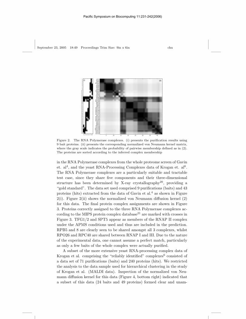
Figure 2. The RNA Polymerase complexes. (i) presents the purification results using9 bait proteins. (ii) presents the corresponding normalized von Neumann kernel matrix,where the gray scale indicates the probability of pairwise membership defined as in (2).The proteins are sorted according to the inferred complex membership

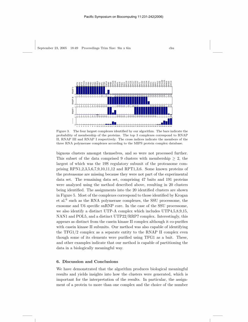
in the RNA Polymerase complexes from the whole proteome screen of Gavinet. al4, and the yeast RNA-Processing Complexes data of Krogan et. al6.The RNA Polymerase complexes are a particularly suitable and tractabletest case, since they share five components and their three-dimensionalstructure has been determined by X-ray crystallography20, providing a“gold standard”. The data set used comprised 9 purifications (baits) and 43proteins (hits) extracted from the data of Gavin et al.4 as shown in Figure2(i). Figure 2(ii) shows the normalized von Neumann diffusion kernel (2)for this data. The final protein complex assignments are shown in Figure3. Proteins correctly assigned to the three RNA Polymerase complexes ac-cording to the MIPS protein complex database21 are marked with crosses inFigure 3. TFG1/2 and SPT5 appear as members of the RNAP II complexunder the APMS conditions used and thus are included in the prediction.RPB5 and 8 are clearly seen to be shared amongst all 3 complexes, whilstRPO26 and RPC40 are shared between RNAP I and III. Due to the natureof the experimental data, one cannot assume a perfect match, particularlyas only a few baits of the whole complex were actually purified.

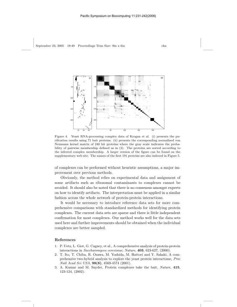
A subset of the more extensive yeast RNA-processing complex data ofKrogan et al. comprising the “reliably identified” complexes6 consisted ofa data set of 71 purifications (baits) and 240 proteins (hits). We restrictedthe analysis to the data sample used for hierarchical clustering in the studyof Krogan et al. (MALDI data). Inspection of the normalized von Neu-mann diffusion kernel for this data (Figure 4, bottom right) indicated thata subset of this data (24 baits and 49 proteins) formed clear and unam-



+ 2 3 + + + + + + + + 12 + 14 + + + 18 19 20 21 22 23 24 25 26 27 28 29 30 31 32 33 34 35 36 37 38 39 40 + 42 430

1

RN

AP

II

SP

T5

AO

S1

SP

T4

RP

O21

TF

G2

RP

B4

RP

B2

TF

G1

RP

B3

RP

B11

RP

B7

IWR

1R

PB

9T

AF

14R

PB

5R

PB

8R

PO

26R

PC

40M

AF

1R

SC

8F

BA

1A

SC

1R

PC

19R

PC

11R

PC

25R

PC

17R

PC

53R

PC

37R

ET

1R

PC

82R

PC

31R

PC

34R

PO

31D

HH

1A

MS

1S

RO

7R

PA

12R

PA

49R

PA

190

RP

A13

5R

PB

10R

PA

43C

DC

14

1 2 3 4 5 6 7 8 9 10 11 12 13 14 + + + + 19 20 21 22 + 24 + 26 27 28 + + + + + 34 35 36 37 38 39 40 + 42 430

1

RN

AP

III

1 2 3 4 5 6 7 8 9 10 11 12 13 14 + + + + 19 20 21 22 + 24 25 26 27 28 29 30 31 32 33 34 35 36 + + + + + + 430

1

RN

AP

I

1 2 3 4 5 6 7 8 9 10 11 12 13 14 15 16 17 18 19 20 21 22 23 24 25 26 27 28 29 30 31 32 33 34 35 36 37 38 39 40 41 42 430

1

−−

−−

−

Figure 3. The four largest complexes identified by our algorithm. The bars indicate theprobability of membership of the proteins. The top 3 complexes correspond to RNAPII, RNAP III and RNAP I respectively. The cross indices indicate the members of thethree RNA polymerase complexes according to the MIPS protein complex database.

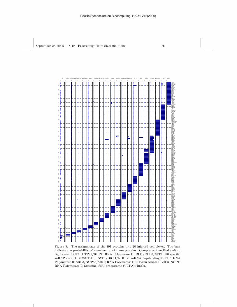
biguous clusters amongst themselves, and so were not processed further.This subset of the data comprised 9 clusters with membership ≥ 2, thelargest of which was the 19S regulatory subunit of the proteasome com-prising RPN1,2,3,5,6,7,9,10,11,12 and RPT1,3,6. Some known proteins ofthe proteasome are missing because they were not part of the experimentaldata set. The remaining data set, comprising 47 baits and 191 proteinswere analyzed using the method described above, resulting in 20 clustersbeing identified. The assignments into the 20 identified clusters are shownin Figure 5. Most of the complexes correspond to those identified by Kroganet al.6 such as the RNA polymerase complexes, the SSU processome, theexosome and U6 specific snRNP core. In the case of the SSU processome,we also identify a distinct UTP-A complex which includes UTP4,5,8,9,15,NAN1 and POL5, and a distinct UTP22/RRP7 complex. Interestingly, thisappears as distinct from the casein kinase II complex although it co-purifieswith casein kinase II subunits. Our method was also capable of identifyingthe TFG1/2 complex as a separate entity to the RNAP II complex eventhough some of its elements were purified using TFG1 as a bait. These,and other examples indicate that our method is capable of partitioning thedata in a biologically meaningful way.

6. Discussion and Conclusions

We have demonstrated that the algorithm produces biological meaningfulresults and yields insights into how the clusters were generated, which isimportant for the interpretation of the results. In particular, the assign-ment of a protein to more than one complex and the choice of the number



20 40 60

50

100

150

200

(i)

50 100 150 200

50

100

150

200

(ii)

Figure 4. Yeast RNA-processing complex data of Krogan et al. (i) presents the pu-rification results using 71 bait proteins. (ii) presents the corresponding normalized vonNeumann kernel matrix of 240 hit proteins where the gray scale indicates the proba-bility of pairwise membership defined as in (2). The proteins are sorted according tothe inferred complex membership. A larger version of the figure can be found on thesupplementary web site. The names of the first 191 proteins are also indexed in Figure 5.

of complexes can be performed without heuristic assumptions, a major im-provement over previous methods.

Obviously, the method relies on experimental data and assignment ofsome artifacts such as ribosomal contaminants to complexes cannot beavoided. It should also be noted that there is no consensus amongst expertson how to identify artifacts. The interpretation must be applied in a similarfashion across the whole network of protein-protein interactions.

It would be necessary to introduce reference data sets for more com-prehensive comparisons with standardized methods for identifying proteincomplexes. The current data sets are sparse and there is little independentconfirmation for most complexes. Our method works well for the data setsused here and further improvements should be obtained when the individualcomplexes are better sampled.

References

1. P. Uetz, L. Giot, G. Cagney, et al., A comprehensive analysis of protein-proteininteractions in Saccharomyces cerevisiae, Nature, 403, 623-627, (2000).

2. T. Ito, T. Chiba, R. Ozawa, M. Yoshida, M. Hattori and Y. Sakaki, A com-prehensive two-hybrid analysis to explore the yeast protein interactome, ProcNatl Acad Sci USA, 98(8), 4569-4574 (2001).

3. A. Kumar and M. Snyder, Protein complexes take the bait, Nature, 415,123-124, (2002).



4. A.C. Gavin, M. Bosche, R. Krause, et al., Functional organization of the yeastproteome by systematic analysis of protein complexes, Nature, 415, 141-147,(2002).

5. Y. Ho, A. Gruhler, A. Heilbut, et al., Systematic identification of proteincomplexes in Saccharomyces cerevisiae by mass spectrometry, Nature, 415,180-183, (2002).

6. N.J. Krogan, W.T. Peng, G. Cagney, et al., High-definition macromolecularcomposition of yeast RNA-processing complexes, Molecular Cell, 13, 225-239,(2004).

7. G. Butland, J. M. Peregrin-Alvarez, J. Li, et al., Interaction network contain-ing conserved and essential protein complexes in Escherichia Coli, Nature,433, 531-537, (2005).

8. G.D. Bader and C.W. Hogue, Analyzing yeast protein-protein interaction dataobtained from different sources, Nat Biotechnol, 20(10), 991-997, (2002).

9. G.D. Bader and C.W. Hogue, An automated method for finding molecularcomplexes in large protein interaction networks, BMC Bioinformatics, 4(1),(2003).

10. V. Spirin and L.A. Mirny, Protein complexes and functional modules inmolecular networks, Proc Natl Acad Sci USA, 100(21), 12123-12128, (2003).

11. J. Hollunder, A. Beyer and T. Wilhelm, Identification and characterizationof protein subcomplexes in yeast, Proteomics, 5(8), 2082-9, (2005).

12. Z. Dezso, Z. Oltvai and A.L. Barabasi, Bioinformatics analysis of experimen-tally determined protein complexes in the Yeast Saccharomyces cerevisiae,Genome Res, 13, 2450-2454, (2003).

13. R. Krause, C. von Mering and P. Bork, A comprehensive set of protein com-plexes in yeast: Mining large scale protein-protein interaction screens, Bioin-formatics, 19(15), 1901-1908, (2003).

14. D. Scholtens and R. Gentleman, Making Sense of High-throughput Protein-protein Interaction Data, Statistical Applications in Genetics and MolecularBiology 3, Article 39, (2004).

15. R. Kondor and J. Lafferty, Diffusion kernels on graphs and other discretestructures, ICML, 315-322, (2002).

16. J. Shawe-Taylor and N. Cristianini, Kernel Methods for Pattern Analysis,(2004).

17. A. Ben-Hur and W.S. Noble, Kernel methods for predicting protein-proteininteractions, Bioinformatics, 21, Suppl. 1, i38-i46, (2005).

18. K. Tsuda and W.S. Noble, Learning kernels from biological networks bymaximizing entropy, Bioinformatics, 20, Suppl. 1, i326-i333, (2004).

19. T. L. Griffiths and Z. Ghahramani, Infinite latent feature models and theIndian buffet process Technical Report, GCNU TR 2005-001, UniversityCollege London, (2005).

20. P. Cramer, D.A. Bushnell, J. Fu, et al., Architecture of RNA polymeraseII and implications for the transcription mechnism, Science, 288, 640-649,(2000).

21. H.W. Mewes, D. Frishman, U. Guldener, et al., MIPS: a database for genomesand protein sequences, Nucleic Acids Res, 30, 31-34, (2002).



0 1

SSB1SSA1KAP123SPT16POB3SSE1HSC82RSC2HSP104SFH1RSC3RSC4RSC9RSC8ARP7STH1NPL6RSC58RSC6ARP9SEC63RSC30SAM1YDJ1SSA2TIF2RTT102PAB1DBP2VMA2RPS0BTCP1UTP9SRO9RVS167YSC85UTP5TUB2CCT4NAP1UTP8UTP4UTP15NAN1POL5PET54LRP1YNR024WYLR339CSKI7SKI6RRP4RRP45RRP6CSL4RRP43RRP40RRP42DIS3RRP46MTR4MTR3SRP1KAP95RPO26RPB5RPS8ARPC40PWP1RPA49RPA34ARC1RNT1CDC16CPR7YCS4CWC22RPA43NOP2RPL7ARPL5RPL2BNSR1RPA190RPA135RPS4BPRP43IMD3NOP1DED1RRP5RPL8ABFR1BMH1HAS1DBP3YGR198WRPS3HCR1NIP1FUN12RPS13RPS1BPRT1RPG1SMC4TIF34RPS17ATIF35TIF5RPS5CDC123CTR9CDC73PAF1RTF1LEO1CKA2CHD1CKA1CKB1CKB2RPO31RPC53RPC37RPC17RPC31RPC34RPC19RET1RPC82LHP1SRP68SRP72RRN3MYO2NOP58SIK1RVB1RVB2TAF14SPT6SPT5RPB4RPB3RPB7RPO21RPB2IML1TIF4631TOP1TDH3YEF3CDC33CDC48YGL245WBRX1NOP12RPL8BRPL15AYPL260WRPL18BSSB2MAM33NPL3CBC2STO1PAT1KEM1YGR054WLSM1RAT1SAP185SIT4RLI1YNL260CRPP0TFG2TFG1RRP7UTP22DST1VPS8RRB1PUS1RPL3MES1RRP8YDR117CTRF4UTP10

RSC2

0 1

UTPA

0 1Exosome

0 1

RNAP I

0 1

NOP1

0 1

elF3

0 1

CK II

0 1

RNAP III

0 1

NOP58/SIK1

0 1

RNAP II

0 1

elF4F

0 1

PWP1

0 1

CBC2/STO1

0 1

snRNP

0 1

SIT4

0 1

RLI1/RPP0

0 1

RNAP II

0 1

UTP22/RRP7

0 1

DST1

510

1520

2530

3540

4550

5560

6570

7580

8590

95100

105110

115120

125130

135140

145150

155160

165170

175180

185190

0 1

20

Figure 5. The assignments of the 191 proteins into 20 inferred complexes. The barsindicate the probability of membership of these proteins. Complexes identified (left toright) are: DST1; UTP22/RRP7; RNA Polymerase II; RLI1/RPP0; SIT4; U6 specificsnRNP core; CBC2/STO1; PWP1/BRX1/NOP12; mRNA cap-binding/EIF4F; RNAPolymerase II; SRP3/NOP58/SIK1; RNA Polymerase III; Casein Kinase II; eIF3; NOP1;RNA Polymerase I; Exosome; SSU processome (UTPA); RSC2.


identifying protein complexes in high-throughput …

Documents