Identifying interfacial molecules in nonplanar interfaces: the generalized ITIM

algorithm

Marcello Sega∗

Tor Vergata University of Rome, via della Ricerca scientifica 1, I-00133 Rome, Italy

Sofia S. KantorovichSapienza University of Rome, p.le A. Moro 4, I-00188 Rome, Italy andUral Federal University, Lenin Ave. 51, 620083 Ekaterinburg, Russia

Pal JedlovszkyLaboratory of Interfaces and Nanosize Systems, Institute of Chemistry,

Eotvos Lorand University, Pazmany stny 1/a, H-1117 Budapest, HungaryMTA-BME Research Group of Technical Analytical Chemistry. Szt. Gellert ter 4, H-1111 Budapest, Hungary and

EKF Department of Chemistry, H-3300 Eger, Leanyka u. 6, Hungary

Miguel JorgeLSRE/LCM-Laboratory of Separation and Reaction Engineering,

Faculdade de Engenharia, Universidade do Porto,Rua Dr. Roberto Frias, 4200-465 Porto, Portugal

We present a generalized version of the itim algorithm for the identification of interfacial molecules,which is able to treat arbitrarily shaped interfaces. The algorithm exploits the similarities betweenthe concept of probe sphere used in itim and the circumsphere criterion used in the α-shapesapproach, and can be regarded either as a reference-frame independent version of the former, oras an extended version of the latter that includes the atomic excluded volume. The new algorithmis applied to compute the intrinsic orientational order parameters of water around a DPC and acholic acid micelle in aqueous environment, and to the identification of solvent-reachable sites infour model structures for soot. The additional algorithm introduced for the calculation of intrinsicdensity profiles in arbitrary geometries proved to be extremely useful also for planar interfaces, asit allows to solve the paradox of smeared intrinsic profiles far from the interface.

I. INTRODUCTION

Capillary waves represent a conceptual problem forthe interpretation of the properties of liquid-liquid orliquid-vapor planar interfaces, because long-wave fluctu-ations are smearing the density profile across the inter-face and all other quantities associated to it. This is usu-ally overcome by calculating the density profile using alocal, instantaneous reference frame located at the inter-face, commonly referred to as the intrinsic density profile,ρ(z) =

⟨

A−1∑

i δ (z − zi + ξ(xi, yi))⟩

, where (xi,yi,zi)is the position of the i-th atom or molecule, and the localelevation of the surface is ξ(xi, yi), assuming the macro-scopic surface normal being aligned with the Z axis of asimulation box with cross section area A. During the lastdecade several numerical methods have been proposedto compute the intrinsic density profiles at interfaces1–6.Despite several differences in these approaches, they are,in general, providing consistent distributions of interfa-cial atoms or molecules6 and density profiles7. Amongthese methods, itim4 proved to be an excellent compro-mise between computational cost and accuracy6, but it islimited to macroscopically flat interfaces, therefore thereis a need to generalize it to arbitrary interfacial shapes.Before these works, albeit for other purposes, several

surface-recognition algorithms have been devised, andwill be briefly mentioned below. All of them are possible

starting points for the sought generalization under thecondition that, once applied to the special case of a pla-nar interface, they lead to consistent results with existingalgorithms for the determination of intrinsic profiles.

Historically, the first class of algorithms addressing theproblem of identifying surfaces was developed to deter-mine molecular areas and volumes. The study of solva-tion properties of molecules and macromolecules (usu-ally, proteins) might require the identification of molecu-lar pockets, or the calculation of the solvent-accessiblesurface area for implicit solvation models8. Two intu-itive concepts are commonly used to describe the surfaceproperties of molecules, namely, that of solvent-accessiblesurface9,10 (SAS), and that of molecular surface11,12 (MS,also known as solvent excluded surface, or Connolly sur-face). The MS can be thought as the surface obtainedby letting a hard sphere roll at close contact with theatoms of the molecule, to generate a smooth surfacemade of a connection of pieces of spheres and tori, whichrepresents the part of the van der Waals surface ex-posed to the solvent. During the process of determin-ing the surface, interfacial atoms can be identified usinga simple geometrical criterion. Many approximated13–24

or analytical11,12,25–30 methods have been developed tocompute the MS or the SAS. In general, these methodsare based on discretization or tessellation procedures, re-quiring therefore the determination of the geometrical

2

structure of the molecule. Other methods which allowto identify molecular surfaces include the approaches ofWillard and Chandler5 or the Circular Variance methodof Mezei31. Incidentally, the way the MS is computed inthe early work of Greer and Bush15 resembles very closelythe itim algorithm4.From the late 1970s, the problem of shape identifica-

tion had started being addressed by a newly born dis-cipline, computational geometry. In this different frame-work, several algorithms have been actively pursued toprovide a workable definition of surface, and in particularthe concept of α-shapes32,33 showed direct implicationsfor the determination of the molecular surfaces34,35. Theapproach based on α-shapes is particularly appealing dueto its generality and ability to describe, besides the ge-ometry, also the intermolecular topology of the system.Prompted by the apparent similarities between the us-

age of the circumsphere in the alpha shapes and that ofthe probe sphere in the itim method, as we will describein the next section, we investigated in more detail theconnection between these two algorithms. As a result, wedeveloped a generalized version of itim (gitim) based onthe α-shapes algorithm. The new gitim method consis-tently reproduces the results of itim in the planar casewhile retaining the ability to describe arbitrarily shapedsurfaces. To the best of our knowledge, the concept ofα-shapes has been employed in the determination of in-trinsic densities at fluid interfaces only once before, byUsabiaga and Duque36, who also noticed the formal sim-ilarities betweeen the α-shapes algorithm and itim.In the following we describe briefly the alpha shapes

and the itim algorithms, explain in detail the general-ization of the latter to arbitrarily shaped surfaces, andpresent several applications.

II. ALPHA SHAPES AND THE GENERALIZED

ITIM ALGORITHM

The concept of α-shapes was introduced severaldecades ago by Edelsbrunner32,33. To date the methodis applied in computer graphics application for digitalshape sampling and processing, in pattern recognitionalgorithms and in structural molecular biology37. Thestarting point in the determination of the surface of aset of points in the α-shapes algorithm is the calculationof the Delaunay triangulation, one of the most fruitfulconcepts for computational geometry38,39, which can bedefined in several equivalent ways, for example, as thetriangulation that maximizes the smallest angle of all tri-angles, or the triangulation of the centers of neighboringVoronoi cells. The idea behind the α-shapes algorithm isto perform a Delaunay triangulation of a set of points,and then generate the so-called α-complex from the unionof all k-simplices (segments, triangles and tetrahedra, forthe simplex dimension k=1,2 and 3, respectively), char-acterized by a k-circumsphere radius (which is the lengthof the segment, the radius of the circumcircle and the ra-

-0.4

-0.2

0

0.2

0.4

-0.4 -0.2 0 0.2 0.4

y / n

m

x / nm

11

22

3333

4444

55

666

7777

8888

9999

10101010

1111

12 12

-0.4

-0.2

0

0.2

0.4

-0.4 -0.2 0 0.2 0.4

y / n

m

x / nm

FIG. 1: Left: example of the α-shapes algorithm on a set ofpoints on the plane. The lines connecting the points representthe Delaunay triangulation (the triangles are labeled by num-bers from 1 to 12). Solid lines mark triangles belonging to theα-complex, and dashed lines those which are not. The light-shaded circles mark those points belonging to the α-shape,which is the border of the α-complex. Two points (in triangle1) are outside the α-shape, and one (shared by triangles 9-12)is inside the α-shape. A circle with the radius of the probedisc α=0.2, with center in triangle 1, is also shown. Right:schematic representation of the itim algorithm, applied to asingle water molecule: the probe spheres (circles) are moveddown the test lines (dashed lines) until they touch an atom.

dius of the circumsphere for k=1,2 and 3, respectively)smaller than a given value, α (hence the name). The α-shape is then defined as the border of the α-complex, andis a polytope which can be, in general, concave, topologi-cally disconnected, and composed of patches of triangles,strings of edges and even sets of isolated points. In apictorial way, one can imagine the α-shape procedure asgrowing probe spheres at every point in space until theytouch the nearest four atoms. These spheres will have, ingeneral, different radii. Those atoms that are touched byspheres with radii larger than the predefined value α areconsidered to be at the surface.

An example of the result of the α-shapes algorithmin two dimensions is sketched in Fig. 1a. The itim al-gorithm is based instead on the idea of selecting thoseatoms of one phase that can be reached by a probe spherewith fixed radius streaming from the other phase alonga straight line, perpendicular to the macroscopic sur-face. An atom is considered to be reached by the probesphere if the two can come at a distance equal to thesum of the probe sphere and Lennard-Jones radii, andno other atom was touched before along the trajectory ofthe probe sphere. In practice, one selects a finite numberof streamlines, and if the space between them is consid-erably smaller than the typical Lennard-Jones radius Rp,the result of the algorithm is practically independent ofthe location and density of the streamlines. The same isnot true regarding the orientation of the streamlines; thisis a direct consequence of the algorithm being designed

3

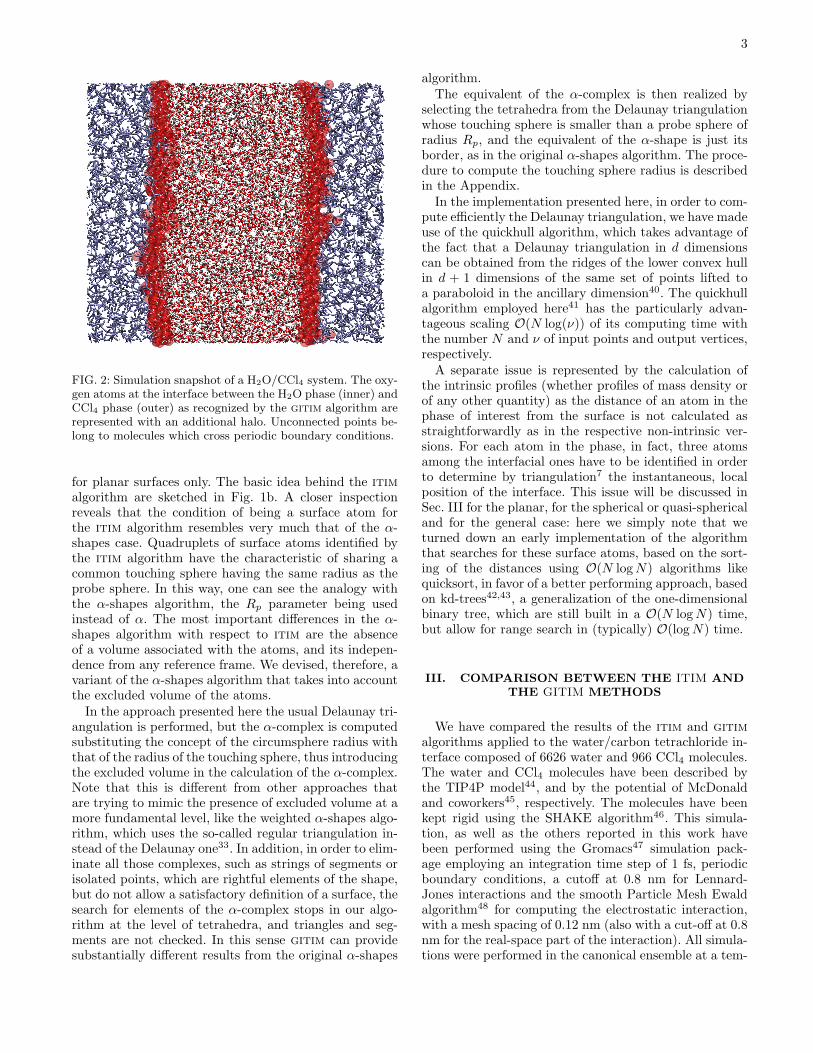
FIG. 2: Simulation snapshot of a H2O/CCl4 system. The oxy-gen atoms at the interface between the H2O phase (inner) andCCl4 phase (outer) as recognized by the gitim algorithm arerepresented with an additional halo. Unconnected points be-long to molecules which cross periodic boundary conditions.

for planar surfaces only. The basic idea behind the itim

algorithm are sketched in Fig. 1b. A closer inspectionreveals that the condition of being a surface atom forthe itim algorithm resembles very much that of the α-shapes case. Quadruplets of surface atoms identified bythe itim algorithm have the characteristic of sharing acommon touching sphere having the same radius as theprobe sphere. In this way, one can see the analogy withthe α-shapes algorithm, the Rp parameter being usedinstead of α. The most important differences in the α-shapes algorithm with respect to itim are the absenceof a volume associated with the atoms, and its indepen-dence from any reference frame. We devised, therefore, avariant of the α-shapes algorithm that takes into accountthe excluded volume of the atoms.In the approach presented here the usual Delaunay tri-

angulation is performed, but the α-complex is computedsubstituting the concept of the circumsphere radius withthat of the radius of the touching sphere, thus introducingthe excluded volume in the calculation of the α-complex.Note that this is different from other approaches thatare trying to mimic the presence of excluded volume at amore fundamental level, like the weighted α-shapes algo-rithm, which uses the so-called regular triangulation in-stead of the Delaunay one33. In addition, in order to elim-inate all those complexes, such as strings of segments orisolated points, which are rightful elements of the shape,but do not allow a satisfactory definition of a surface, thesearch for elements of the α-complex stops in our algo-rithm at the level of tetrahedra, and triangles and seg-ments are not checked. In this sense gitim can providesubstantially different results from the original α-shapes

algorithm.The equivalent of the α-complex is then realized by

selecting the tetrahedra from the Delaunay triangulationwhose touching sphere is smaller than a probe sphere ofradius Rp, and the equivalent of the α-shape is just itsborder, as in the original α-shapes algorithm. The proce-dure to compute the touching sphere radius is describedin the Appendix.In the implementation presented here, in order to com-

pute efficiently the Delaunay triangulation, we have madeuse of the quickhull algorithm, which takes advantage ofthe fact that a Delaunay triangulation in d dimensionscan be obtained from the ridges of the lower convex hullin d + 1 dimensions of the same set of points lifted toa paraboloid in the ancillary dimension40. The quickhullalgorithm employed here41 has the particularly advan-tageous scaling O(N log(ν)) of its computing time withthe number N and ν of input points and output vertices,respectively.A separate issue is represented by the calculation of

the intrinsic profiles (whether profiles of mass density orof any other quantity) as the distance of an atom in thephase of interest from the surface is not calculated asstraightforwardly as in the respective non-intrinsic ver-sions. For each atom in the phase, in fact, three atomsamong the interfacial ones have to be identified in orderto determine by triangulation7 the instantaneous, localposition of the interface. This issue will be discussed inSec. III for the planar, for the spherical or quasi-sphericaland for the general case: here we simply note that weturned down an early implementation of the algorithmthat searches for these surface atoms, based on the sort-ing of the distances using O(N logN) algorithms likequicksort, in favor of a better performing approach, basedon kd-trees42,43, a generalization of the one-dimensionalbinary tree, which are still built in a O(N logN) time,but allow for range search in (typically) O(logN) time.

III. COMPARISON BETWEEN THE ITIM AND

THE GITIM METHODS

We have compared the results of the itim and gitim

algorithms applied to the water/carbon tetrachloride in-terface composed of 6626 water and 966 CCl4 molecules.The water and CCl4 molecules have been described bythe TIP4P model44, and by the potential of McDonaldand coworkers45, respectively. The molecules have beenkept rigid using the SHAKE algorithm46. This simula-tion, as well as the others reported in this work havebeen performed using the Gromacs47 simulation pack-age employing an integration time step of 1 fs, periodicboundary conditions, a cutoff at 0.8 nm for Lennard-Jones interactions and the smooth Particle Mesh Ewaldalgorithm48 for computing the electrostatic interaction,with a mesh spacing of 0.12 nm (also with a cut-off at 0.8nm for the real-space part of the interaction). All simula-tions were performed in the canonical ensemble at a tem-

4

0

100

200

300

400

500

600

0.1 0.2 0.3 0.4 0.5 0.6

Ave

rage

num

ber

of s

urfa

ce a

tom

s

Probe sphere radius / nm

ITIMGITIM

FIG. 3: Average number of surface atoms identified by itim

(squares) and gitim (circles) as a function of the probe sphereradius.

perature of 300K using the Nose–Hoover thermostat49,50

with a relaxation time of 0.1 ps. A simulation snapshot ofthe H2O/CCl4 interface is presented in Fig. 2, where thesurface atoms identified by the gitim algorithm using aprobe sphere radius of 0.25 nm are highlighted using aspherical halo.We have used the itim and gitim algorithms to iden-

tify the interfacial atoms of the water phase in the sys-tem, for different sizes of the probe sphere. In general,gitim identifies systematically a larger number of inter-facial atoms than itim for the same value of the probesphere radius Rp, as it is clearly seen in Fig. 3. Remark-ably, for values of the probe sphere radius smaller thanabout 0.2 nm (compare, for example, with the optimalitim parameter Rp = 0.125 nm suggested in Ref. 6),the interfacial atoms identified by gitim show the onsetof percolation. The reason for this behavior traces backto the fact that itim is unable to identify voids buriedin the middle of the phase, as it is effectively probingonly the cross section of the voids along the direction ofthe streamlines. This difference could explain the highernumber of surface atoms identified by gitim, as voids ina region with high local curvature (or, in other words,with a local surface normal which deviates significantlyfrom the macroscopic one) will not be identified as suchby itim. In gitim, on the contrary, probe spheres canbe thought as inflating at every point in space instead ofmoving down the streamlines, and this is the reason whythe algorithm is able to identify also small pockets insidethe opposite phase.It is possible to make a rough but enlightening an-

alytical estimate of the probability for a probe sphereof null radius in the itim algorithm to penetrate for adistance ζ in a fluid of hard spheres with diameter σand number density ρ. Using the very crude approxima-tion of randomly distributed spheres, the probability p0to pass the first molecular layer, at a depth ζ = σ isthe effective cross section p0 = 1 − π

4ρ2/3σ2, and that

FIG. 4: Water surface oxygen atoms in the H2O/CCl4 systemin one simulation snapshot as recognized by gitim exclusively(small spheres), itim exclusively (large spheres) or by bothmethods (sphere with halo).

of reaching a generic depth ζ can be approximated as

p(ζ) = pζ/σ0 , where κ = ln(1/p0)/σ defines a penetra-

tion depth. Therefore, using a probe sphere with a nullradius, itim will identify a (diffuse) surface at a depth1/κ, while gitim will identify every atom as a surfaceone. For water at ambient conditions, the penetration isκ−1 ≃ 0.186 nm, a distance smaller than the size of a wa-ter molecule itself. This could explain why in Ref. 6, evenusing a probe sphere radius as small as 0.05 nm, almostonly water molecules in the first layer were identified asinterfacial ones by itim (see the almost perfectly Gaus-sian distribution of interfacial water molecules in Fig.9 ofRef. 6).Nevertheless, it is important for practical reasons to be

able to match the outcome of both algorithms. It turnsout that choosing Rp so that the average number of inter-facial atoms identified by both algorithms is roughly thesame leads also, not surprisingly, to very similar distribu-tions. The probe sphere radius required for gitim to ob-tain a similar average number of surface atom as in itim

can be obtained by an interpolation of the values reportedin Fig. 3. An example showing explicitly the interfacialatoms identified by the two methods (Rp = 0.2 nm foritim and Rp = 0.25 nm for gitim) is presented in Fig. 4:roughly 85% of surface atoms are identified simultane-ously by both methods, demonstrating the good agree-ment between the two methods once the probe sphereradius has been re-gauged. The condition of identifyingthe same atoms as interfacial ones is much more strictthat any condition on average quantities, like the spatialdistribution of interfacial atoms or intrinsic density pro-files. Hence, it is expected that a good agreement on suchquantities can also be achieved.The intrinsic density profiles of water and carbon tetra-

chloride are reported in Fig. 5, as computed by itim and

5

0

500

1000

1500

2000

2500

3000

3500

-2 -1 0 1 2 3

Den

sity

/ (k

g / m

3 )

Position relative to the interface / nm

ITIM (H2O)GITIM (H2O)ITIM (CCl4)GITIM (CCl4)GTIM+MC (CCl4)GTIM+MC (H2O)GTIM (CCl4, big)

FIG. 5: Intrinsic density profiles of water (curves on the left)and carbon tetrachloride (curves on the right) with respect tothe water surface as computed with itim (thick, solid lines)or with gitim (thick, dotted lines). The profile computed us-ing gitim and the Monte Carlo normalization procedure de-scribed in Sec. IV are also shown (thin, solid lines), as wellas the one for carbon tetrachloride computed in the biggersystem (thin, dashed line) using gitim and no Monte Carlonormalization.

gitim, respectively, with the interfacial water moleculesas reference. The procedure for identifying the local dis-tance of an atom from the surface is in its essence thesame as described in Ref. 7. Starting from the projec-tion P0 = (x, y) of the position of the given atom to themacroscopic interface plane, the two interfacial atomsclosest to P0 are found (their position on the interfaceplane being P1 and P2, respectively). The third closestatom with projection P3 has then to be found, with thecondition that the triangle P1P2P3 contains the point P0.A linear interpolation of the elevation of P0 from those ofthe other points is eventually performed, and employed tocompute the distance z−ξ(x, y) which is used to computethe intrinsic density profile. Efficient neighbor search forthe P1, P2 and candidate P3 atoms is implemented usingkd-trees43 as discussed before. The two pairs of profilesare very similar, besides a small difference in the positionand height of the main peak of the CCl4 profile (curveson the right in Fig. 5) and in the minimum of the waterprofile (curves on the left in Fig. 5) next to the surface po-sition, which are anyway compatible with the differencesobserved between various methods for the calculation ofintrinsic density profiles7. The delta-like contribution ofthe water molecules at the surface is included in the plotin Fig. 5, and defines the origin of the reference system.Negative values of the signed distance from the interfacecorrespond to the aqueous phase.

IV. THE PROBLEM OF NORMALIZATION OF

DENSITY PROFILES

Before applying gitim to non-planar interfaces, oneimportant issue has still to be solved, namely that ofthe proper calculation of intrinsic density profiles in non-planar geometries. In general, one uses one-dimensionaldensity profiles (intrinsic or non-intrinsic) when the sys-tem is, or is assumed to be, invariant under displace-ments along the interface, so that the orthogonal degreesof freedom can be integrated out. When the interface hasa non-planar shape, one needs to use a different coordi-nate system.

For the sake of simplicity we will refer now to the spher-ical or quasi-spherical case, but the following considera-tions apply to any other coordinate system. To computethe non-intrinsic density profile with respect to an objectwhose surface is fluctuating but is on average spherical,one can use the spherical coordinate system and normal-ize each bin by the integral of the Jacobian determinant,that is the volume of the shell at constant distance fromthe origin. In the intrinsic case, however, the istantaneousvolume of the shell at constant distance from the intrin-sic surface of the object is different from the sphericalshell volume. Atoms at the same distance from the in-trinsic surface might be associated to different sphericalshells, with correspondingly different values of the Jaco-bian, thus introducing unwanted artefacts. An exampleof how this normalization affects the calculation of thedensity profile will be presented in Sec.VA.

To avoid these problems, one needs to provide a propernormalization by calculating at every frame the volumeof shells at constant intrinsic distance. In principle, thiscould be calculated by ordinary numerical integration,but this would require a large computing time and stor-age overhead. Here, instead, we propose to employ anapproach based on simple Monte Carlo integration: inparallel with the calculation of the histograms for thevarious phases, we compute also that of a random dis-tribution of points, equal in number to the total atomsin the simulation. The volume of a shell can then be es-timated as the ratio of the number of points found at agiven distance and the total number of random pointsdrawn, times the volume of the simulation box. We arefollowing the heuristic idea that for each frame j one doesnot need to know the volume of the shell Vj(r) with a pre-cision higher than that of the average number of atomsin it, nj(r). In addition, we assume that the surface areaof the interface is large enough for the shell volume varia-tions δVj(r) to be small with respect to its average value

V (r) =∑T

j Vj(r)/T .

The average intrinsic number density profile

ρ(r) =1

T

T∑

j=1

nj(r)

Vj(r)(1)

can therefore be approximated using a Taylor expansion

6

as

ρ(r) ≃1

T

1

V (r)

T∑

j=1

[

nj(r)− nj(r)δVj(r)

V (r)

]

=n(r)

V (r)

[

1 +O(

δVj(r)/V (r))]

. (2)

When the relative volume changes |δV/V | are small, onecan therefore simply normalize the histogram n(r) =∑T

j nj(r)/n by the average volume V (r) obtained by theMonte Carlo procedure, disregarding the terms of orderO(δV/V ).The correctness of our assumption is demonstrated in-

cidentally by the application of this normalization onceagain to the planar case. The thin lines in Fig. 5 repre-sent the itim intrinsic mass density profile of water andcarbon tetrachloride, using the Monte Carlo normaliza-tion scheme instead of the usual normalization with boxcross sectional area and slab width. Close to the inter-face, the Monte Carlo normalization gives results whichare fully compatible with the usual method, showing thatthe accuracy of the volume estimate is adequate. On theother hand one can see that far from the interface thetwo profiles behave quite differently.The profile computed with usual normalization decays

slowly to zero when approaching the distance of roughlyhalf a box length. This is because the minimum imageconvention is used, in conjunction with periodic bound-ary conditions, to determine the distance of one particlefrom the (nearest) interface. The maximum distance fromthe surface that a point can attain depends therefore onthe local thickness of the slab. Where the slab is thickerthe maximum allowed distance is smaller than in regionswhere the slab is thinner. Because of this purely geomet-ric artefact, particles at large distances (close to half asimulation box minus the average slab thickness) will be-come more unlikely with increasing distance of the pointfrom the surface, leading to a smoothly vanishing den-sity profile, even though on physical grounds one wouldexpect a constant one.The case with Monte Carlo normalization, on the con-

trary, shows that it is possible to reach the expectedconstant density profile at large distances. The use ofMonte Carlo normalization appears to change some fea-tures of the profile, such as the heigth of the thrid peakat about 1.5 nm, and reveals new ones such as a smallfourth peak around 2 nm. To check that the Monte Carlonormalization is revealing indeed physical properties andnot some artefacts, we performed a new simulation withlarger width of both the water and the carbon tetrachlo-ride slabs (9746 and 1566 water and carbon tetrachloridemolecules, respectively), and we calculated the densityprofile without the Monte Carlo normalization. The re-sulting profile agrees with the one computed with the aidof the Monte Carlo normalization in the smaller system(see 5), confirming the correctness of the Monte Carlonormalization and its ability to extract relevant informa-tion in poorly sampled regions.

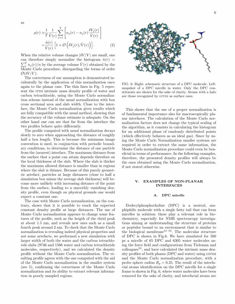
FIG. 6: Right: schematic structure of a DPC molecule. Left:snapshot of a DPC micelle in water. Only the DPC con-stituents are shown for the sake of clarity. Atoms with a haloare those recognized by gitim as surface ones.

This shows that the use of a proper normalization isof fundamental importance also for macroscopically pla-nar interfaces. The calculation of the Monte Carlo nor-malization factors does not change the typical scaling ofthe algorithm, as it consists in calculating the histogramfor an additional phase of randomly distributed points(which effectively behaves as an ideal gas). Since by us-ing the Monte Carlo Normalization smaller systems arerequired in order to extract the same information, theMonte Carlo normalization procedure could even be ben-eficial in terms of performance. In the following examples,therefore, the presented density profiles will always bethe ones obtained using the Monte Carlo normalization,if not stated otherwise.

V. EXAMPLES OF NON-PLANAR

INTERFACES

A. DPC micelle

Dodecylphosphocholine (DPC) is a neutral, am-phiphilic molecule with a single fatty tail that can formmicelles in solution: these play a relevant role in bio-chemistry, especially for NMR spectroscopy investiga-tions aiming at understanding the structure of proteinsor peptides bound to an environment that is similar tothe biological membrane51–54. The molecular structureof DPC is shown in Fig.6. We have simulated for 500ps a micelle of 65 DPC and 6305 water molecules us-ing the force field and configurations from Tieleman andcolleagues55, and have calculated the intrinsic mass den-sity profiles of both phases (DPC and water) using gitim

and the Monte Carlo normalization procedure, with aprobe sphere radius Rp = 0.25. The result of the interfa-cial atoms identification on the DPC micelle for a singleframe is shown in Fig. 6, where water molecules have beenremoved for the sake of clarity, and interfacial atoms are

7

0

500

1000

1500

Den

sity

/kg

m-3

DPCWater

0

500

1000

1500

Den

sity

/kg

m-3

Monte Carlo norm.Spherical norm.

RDFDistance from P

-0.3-0.2-0.1

0 0.1 0.2

-1.2 -0.8 -0.4 0.0 0.4 0.8 1.2

Ord

er p

aram

eter

distance from the interface / nm

<cos(θ1)><3cos2(θ2)-1>/2

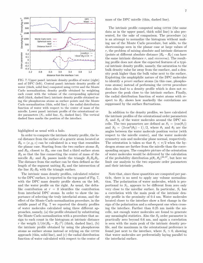
FIG. 7: Upper panel: intrinsic density profiles of water (right)and of DPC (left). Central panel: intrinsic density profile ofwater (thick, solid line) computed using gitim and the MonteCarlo normalization; density profile obtained by weightingeach count with the volume of the correponding sphericalshell (thick, dashed line); intrinsic density profile obtained us-ing the phosphorous atoms as surface points and the MonteCarlo normalization (thin, solid line) ; the radial distributionfunction of water with respect to the center of mass of themicelle. Lower panel: intrinsic profile of the orientational or-der parameters (S1, solid line, S2, dashed line). The verticaldashed lines marks the position of the interface.

highlighted as usual with a halo.

In order to compute the intrinsic density profile, the lo-cal distance from the surface of a generic atom located atR0 = (x, y, z) can be calculated in a way that resemblesthe planar case. Starting from the two surface atoms R1

and R2, closest to R0, one can find a third surface atomR3 so that the line connecting the center of mass of themicelle RC and R0 passes inside the triangle R1R2R3.The distance from the surface can be then defined as thelength of the segment uniting R0 and the intersection ofthe line RCR0 with the triangle surface.

The intrinsic mass density profiles, calculated relativeto the DPC surface, is reported in the top panel of Fig. 7,with the DPC mass density profile shown on the left,and the water profile on the right. As usual, the delta-like contribution at r = 0 identifies the contributionfrom interfacial DPC atoms. In order to show the im-portance of selecting the truly interfacial atoms, and theeffect of the Monte Carlo normalization procedure, in themiddle panel of Fig. 7 we reported the density profilesof water molecules calculated using three different ap-proaches, namely, (a) the profile obtained by substitutingthe Monte Carlo normalization with a procedure that as-sign to each count in the histogram at intrinsic distancer the weigth 1/(4π|R0 − RC |

2) (thick, dashed line), (b)the intrinsic profile obtained by using the phosphorousatoms as surface atoms instead or relying on the gitim

approach (thin, solid line), and (c) the radial distributionfunction of water calculated with respect to the center of

mass of the DPC micelle (thin, dashed line).

The intrinsic profile computed using gitim (the samedata as in the upper panel, thick solid line) is also pre-sented, for the sake of comparison. The procedure (a)is an attempt to normalize the histogram without mak-ing use of the Monte Carlo procedure, but adds, to theshortcomings seen in the planar case at large values ofr, the problem of mixing absolute and intrinsic distances(points at different absolute distance |R0−RC | can havethe same intrinsic distance r, and viceversa). The result-ing profile does not show the expected features of a typi-cal intrinsic density profile, namely, the saturation to thebulk density value far away from the susrface, and a den-sity peak higher than the bulk value next to the surface.Exploiting the amphiphilic nature of the DPC moleculesto identify a priori surface atoms (in this case, phospho-rous atoms) instead of performing the gitim proceduredoes also lead to a density profile which is does not re-produce the peak close to the intrinsic surface. Finally,the radial distribution function of water atoms with re-spect to RC shows how markedly the correlations aresuppressed by the surface fluctuations.

In addition to the density profiles, we have calculatedthe intrinsic profiles of the orientational order parametersS1 and S2 of the water molecules around the DPC mi-celle. The two parameters are defined as S1 = 〈cos(θ1)〉and S2 =

⟨

3 cos2(θ2)− 1⟩

/2, where θ1 and θ2 are theangles between the water molecule position vector (withrespect to the micelle center), and the water moleculesymmetry axis and molecular plane normal, respectively.The orientation is taken so that θ1 < π/2 when the hy-drogen atoms are farther from the micelle than the corre-sponding oxygen. The complete picture of the orientationof water molecules would be delivered by the calculationof the probability distribution p(θ1, θ2)

56,57, but here welimit our analysis to the two separate order parametersand their intrinsic profiles.

Note that, since these quantities are computed per par-ticle, there is no need to apply any volume normaliza-tion. The polarization of water molecules, which is pro-portional to S1, appears to be different from zero onlyvery close to the micellar surface. In particular, S1 hasa correlation with the main peak of the intrinsic den-sity profile in the proximity of 0.4 nm. Water moleculeslocated closer to the interface show a first change in thesign of the polarization and a subsequent one when cross-ing the interface. Farther than 0.25 nm inside the mi-celle, not enough water molecules are found to generateany meaningful statistics. Also the S2 order parameter ispractically zero beyond 0.6 nm, and again a correlationis seen with the main peak of the intrinsic density pro-file, and the maximum in the orientational preference isfound just next to the interface, where S1 ≃ 0, showingthat water molecules are preferentially laying parallel tothe interfacial surface.

8

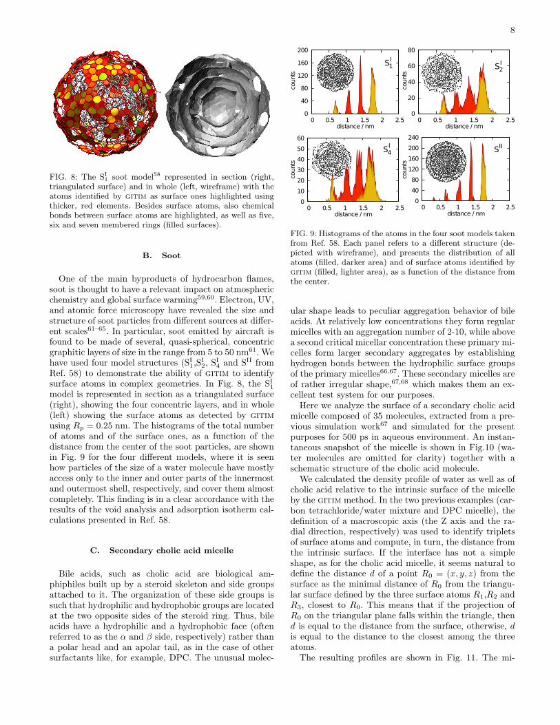
FIG. 8: The SI

1 soot model58 represented in section (right,triangulated surface) and in whole (left, wireframe) with theatoms identified by gitim as surface ones highlighted usingthicker, red elements. Besides surface atoms, also chemicalbonds between surface atoms are highlighted, as well as five,six and seven membered rings (filled surfaces).

B. Soot

One of the main byproducts of hydrocarbon flames,soot is thought to have a relevant impact on atmosphericchemistry and global surface warming59,60. Electron, UV,and atomic force microscopy have revealed the size andstructure of soot particles from different sources at differ-ent scales61–65. In particular, soot emitted by aircraft isfound to be made of several, quasi-spherical, concentricgraphitic layers of size in the range from 5 to 50 nm61. Wehave used four model structures (SI1,S

I2, S

I4 and SII from

Ref. 58) to demonstrate the ability of gitim to identifysurface atoms in complex geometries. In Fig. 8, the SI1model is represented in section as a triangulated surface(right), showing the four concentric layers, and in whole(left) showing the surface atoms as detected by gitim

using Rp = 0.25 nm. The histograms of the total numberof atoms and of the surface ones, as a function of thedistance from the center of the soot particles, are shownin Fig. 9 for the four different models, where it is seenhow particles of the size of a water molecule have mostlyaccess only to the inner and outer parts of the innermostand outermost shell, respectively, and cover them almostcompletely. This finding is in a clear accordance with theresults of the void analysis and adsorption isotherm cal-culations presented in Ref. 58.

C. Secondary cholic acid micelle

Bile acids, such as cholic acid are biological am-phiphiles built up by a steroid skeleton and side groupsattached to it. The organization of these side groups issuch that hydrophilic and hydrophobic groups are locatedat the two opposite sides of the steroid ring. Thus, bileacids have a hydrophilic and a hydrophobic face (oftenreferred to as the α and β side, respectively) rather thana polar head and an apolar tail, as in the case of othersurfactants like, for example, DPC. The unusual molec-

FIG. 9: Histograms of the atoms in the four soot models takenfrom Ref. 58. Each panel refers to a different structure (de-picted with wireframe), and presents the distribution of allatoms (filled, darker area) and of surface atoms identified bygitim (filled, lighter area), as a function of the distance fromthe center.

ular shape leads to peculiar aggregation behavior of bileacids. At relatively low concentrations they form regularmicelles with an aggregation number of 2-10, while abovea second critical micellar concentration these primary mi-celles form larger secondary aggregates by establishinghydrogen bonds between the hydrophilic surface groupsof the primary micelles66,67. These secondary micelles areof rather irregular shape,67,68 which makes them an ex-cellent test system for our purposes.Here we analyze the surface of a secondary cholic acid

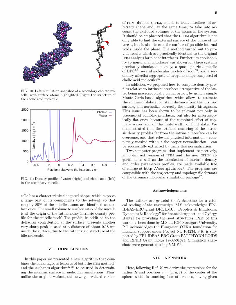
micelle composed of 35 molecules, extracted from a pre-vious simulation work67 and simulated for the presentpurposes for 500 ps in aqueous environment. An instan-taneous snapshot of the micelle is shown in Fig.10 (wa-ter molecules are omitted for clarity) together with aschematic structure of the cholic acid molecule.We calculated the density profile of water as well as of

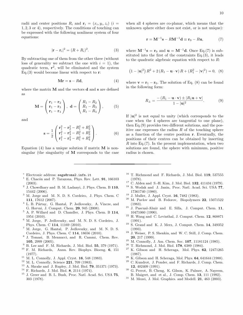
cholic acid relative to the intrinsic surface of the micelleby the gitim method. In the two previous examples (car-bon tetrachloride/water mixture and DPC micelle), thedefinition of a macroscopic axis (the Z axis and the ra-dial direction, respectively) was used to identify tripletsof surface atoms and compute, in turn, the distance fromthe intrinsic surface. If the interface has not a simpleshape, as for the cholic acid micelle, it seems natural todefine the distance d of a point R0 = (x, y, z) from thesurface as the minimal distance of R0 from the triangu-lar surface defined by the three surface atoms R1,R2 andR3, closest to R0. This means that if the projection ofR0 on the triangular plane falls within the triangle, thend is equal to the distance from the surface, otherwise, dis equal to the distance to the closest among the threeatoms.The resulting profiles are shown in Fig. 11. The mi-

9

FIG. 10: Left: simulation snapshot of a secondary cholate mi-celle, with surface atoms highlighted. Right: the structure ofthe cholic acid molecule.

0

500

1000

1500

2000

2500

-0.4 -0.2 0 0.2 0.4 0.6 0.8 1

Den

sity

/ (

kg /

m3 )

Position relative to the interface / nm

CholateWater

FIG. 11: Density profile of water (right) and cholic acid (left)in the secondary micelle.

celle has a characteristic elongated shape, which exposesa large part of its components to the solvent, so thatroughly 80% of the micelle atoms are identified as sur-face ones. The small volume to surface ratio of the micelleis at the origin of the rather noisy intrinsic density pro-file for the micelle itself. The profile, in addition to thedelta-like contribution at the surface, presents anothervery sharp peak located at a distance of about 0.18 nminside the surface, due to the rather rigid structure of thebile molecule.

VI. CONCLUSIONS

In this paper we presented a new algorithm that com-bines the advantageous features of both the itimmethod4

and the α-shapes algorithm32,33 to be used in determin-ing the intrinsic surface in molecular simulations. Thus,unlike the original variant, this new, generalized version

of itim, dubbed gitim, is able to treat interfaces of ar-bitrary shape and, at the same time, to take into ac-count the excluded volumes of the atoms in the system.It should be emphasized that the gitim algorithm is notonly able to find the external surface of the phase of in-terest, but it also detects the surface of possible internalvoids inside the phase. The method turned out to pro-vide results which are practically identical to the originalitim analysis for planar interfaces. Further, its applicabil-ity to non-planar interfaces was shown for three systemspreviously simulated, namely, a quasi-spherical micelleof DPC55, several molecular models of soot58, and a sec-ondary micellar aggregate of irregular shape composed ofcholic acid molecules67.In addition, we proposed how to compute density pro-

files relative to intrinsic interfaces, irrespective of the lat-ter being macroscopically planar or not, by using a simpleMonte Carlo-based algorithm, which allows to estimatethe volume of slabs at constant distance from the intrinsicsurface, and normalize correctly the density histograms.This issue has been shown to be relevant not only inpresence of complex interfaces, but also for macroscop-ically flat ones, because of the combined effect of cap-illary waves and of the finite width of fluid slabs. Wedemonstrated that the artificial smearing of the intrin-sic density profiles far from the intrinsic interface can beovercome, and that relevant physical information – com-pletely masked without the proper normalization – canbe successfully extracted by using this normalization.Two computer programs that implement, respectively,

an optimized version of itim and the new gitim al-gorithm, as well as the calculation of intrinsic densityand order parameters profiles, are made available freeof charge at http://www.gitim.eu/. The programs arecompatible with the trajectory and topology file formatsof the Gromacs molecular simulation package47.

Acknowledgements

The authors are grateful to F. Sciortino for a criti-cal reading of the manuscript. M.S. acknowledges FP7-IDEAS-ERC grant DROEMU: “Droplets & Emulsions:Dynamics & Rheology” for financial support, and GyorgyHantal for providing the soot structures. Part of thiswork has been done by M.S. at ICP, Stuttgart University.P.J. acknowledges the Hungarian OTKA foundation forfinancial support under Project Nr. 104234. S.K. is sup-ported by FP7-IDEAS-ERC Grant PATCHYCOLLOIDSand RFBR Grant mol a 12-02-31374. Simulation snap-shots were generated using VMD69.

VII. APPENDIX

Here, following Ref. 70 we derive the expressions for theradius R and position r = (x, y, z) of the center of thesphere which is touching four other ones, having given

10

radii and center positions Ri and ri = (xi, yi, zi) (i =1, 2, 3 or 4), respectively. The conditions of touching canbe expressed with the following nonlinear system of fourequations:

|r− ri|2 = (R+Ri)

2. (3)

By subtracting one of them from the other three (withoutloss of generality we subtract the one with i = 1), thequadratic term, r

2, will be eliminated and the systemEq.(3) would become linear with respect to r:

Mr = s−Rd, (4)

where the matrix M and the vectors d and s are definedas

M =

r1 − r2

r1 − r3

r1 − r4

, d =

R1 −R2

R1 −R3

R1 −R4

, (5)

and

s =1

2

r21 − r

22 −R2

1 +R22

r21 − r

23 −R2

1 +R23

r21 − r

24 −R2

1 +R24

. (6)

Equation (4) has a unique solution if matrix M is non-singular (the singularity of M corresponds to the case

when all 4 spheres are co-planar, which means that theunknown sphere either does not exist, or is not unique):

r = M−1

s−RM−1

d ≡ r0 −Ru, (7)

where M−1

s = r0 and u = M−1

d. Once Eq.(7) is sub-stituted into the first of the constraints Eq.(3), it leadsto the quadratic algebraic equation with respect to R:

(

1− |u|2)

R2 + 2 (R1 − u · v)R+ (R21 − |v|2) = 0, (8)

where v = r1 − r0. The solution of Eq. (8) can be foundin the following form:

R± =− (R1 − u · v)± |R1u+ v|

1− |u|2. (9)

If |u|2 is not equal to unity (which corresponds to thecase when the 4 spheres are tangential to one plane),then Eq.(9) provides two different solutions, and the pos-itive one expresses the radius R of the touching sphereas a function of the centre position r. Eventually, thepositions of their centres can be obtained by insertingR into Eq.(7). In the present implementation, when twosolutions are found, the sphere with minimum, positiveradius is chosen.

∗ Electronic address: sega@roma2.infn.it1 E. Chacon and P. Tarazona, Phys. Rev. Lett. 91, 166103(2003).

2 J. Chowdhary and B. M. Ladanyi, J. Phys. Chem. B 110,15442 (2006).

3 M. Jorge and M. N. D. S. Cordeiro, J. Phys. Chem. C111, 17612 (2007).

4 L. B. Partay, G. Hantal, P. Jedlovszky, A. Vincze, andG. Horvai, J. Comput. Chem. 29, 945 (2008).

5 A. P. Willard and D. Chandler, J. Phys. Chem. B 114,1954 (2010).

6 M. Jorge, P. Jedlovszky, and M. N. D. S. Cordeiro, J.Phys. Chem. C 114, 11169 (2010).

7 M. Jorge, G. Hantal, P. Jedlovszky, and M. N. D. S.Cordeiro, J. Phys. Chem. C 114, 18656 (2010).

8 J. Tomasi, B. Mennucci, and R. Cammi, Chem. Rev.105, 2999 (2005).

9 B. Lee and F. M. Richards, J. Mol. Biol. 55, 379 (1971).10 F. M. Richards, Annu. Rev. Biophys. Bioeng. 6, 151

(1977).11 M. L. Connolly, J. Appl. Cryst. 16, 548 (1983).12 M. L. Connolly, Science 221, 709 (1983).13 A. Shrake and J. Rupley, J. Mol. Biol. 79, 351371 (1973).14 F. Richards, J. Mol. Biol. 8, 2114 (1974).15 J. Greer and B. L. Bush, Proc. Natl. Acad. Sci. USA 75,

303 (1978).

16 T. Richmond and F. Richards, J. Mol. Biol. 119, 537555(1978).

17 C. Alden and S.-H. Kim, J. Mol. Biol. 132, 411434 (1979).18 S. Wodak and J. Janin, Proc. Natl. Acad. Sci. USA 77,

17361740 (1980).19 J. Muller, J. Appl. Cryst. 16, 7482 (1983).20 M. Pavlov and B. Fedorov, Biopolymers 22, 15071522

(1983).21 J. Pascual-Ahuir and E. Silla, J. Comput. Chem. 11,

10471060 (1990).22 H. Wang and C. Levinthal, J. Comput. Chem. 12, 868871

(1991).23 S. Grand and K. J. Merz, J. Comput. Chem. 14, 349352

(1993).24 J. Weiser, P. S. Shenkin, and W. C. Still, J. Comp. Chem.

20, 217 (1999).25 M. Connolly, J. Am. Chem. Soc. 107, 11181124 (1985).26 T. Richmond, J. Mol. Biol. 178, 6389 (1984).27 K. Gibson and H. Scheraga, Mol. Phys. 62, 12471265

(1987).28 K. Gibson and H. Scheraga, Mol. Phys. 64, 641644 (1988).29 C. Kundrot, J. Ponder, and F. Richards, J. Comp. Chem.

12, 402409 (1991).30 G. Perrot, B. Cheng, K. Gilson, K. Palmer, A. Nayeem,

B. Maigret, and et al., J. Comp. Chem. 13, 111 (1992).31 M. Mezei, J. Mol. Graphics. and Modell. 21, 463 (2003).

11

32 H. Edelsbrunner, D. Kirkpatrick, and R. Seidel, IEEETrans. on Information Theory 29, 551 (1983).

33 H. Edelsbrunner and E. Mucke, ACM T. Graphic. 13, 43(1994).

34 H. Edelsbrunner, M. Facello, P. Fu, and J. Liang, Mea-suring proteins and voids in proteins, in Proc. 28th Annu.Hawaii Intl. Conf. System Sciences, volume 5, p. 256264,Los Alamitos, California, 1995, IEEE Computer SocietyPress.

35 J. Liang, H. Edelsbrunner, P. Fu, P. V. Sudhakar, andS. Subramanian, Proteins 33, 1 (1998).

36 F. Usabiaga and D. Duque, Physical Review E 79, 046709(2009).

37 H. Edelsbrunner, Handbook of Discrete and ComputationalGeometry, edited by J. E. Goodman and J. O’Rourke, chap-ter 63, pp. 1395–1412, CRC Press, Boca Raton, Florida,2004.

38 B. N. Delaunay, Izv. Akad. Nauk SSSR, Otdelenie Matem-aticheskii i Estestvennyka Nauk 7, 793800 (1934).

39 A. Okabe, B. Boots, K. Sugihara, and S. N. Chiu, Spa-tial Tessellations: Concepts and Applications of VoronoiDiagrams, Wiley, Chichester, U.K., 2000.

40 D. Brown, Inf. Process. Lett. 9, 223228 (1979).41 C. Barber, D. Dobkin, and H. Huhdanpaa, ACM T.

Math. Software 22, 469 (1996).42 J. L. Bentley, Cmmun. ACM 18, 509 (1975).43 J. Bentley and J. Friedman, ACM Compu. Sur. 11, 397

(1979).44 W. L. Jorgensen, J. Chandrashekar, J. D. Madura, R. Im-

pey, and M. L. J. Klein, Chem. Phys. 79, 926 (1983).45 I. R. McDonald, D. G. Bounds, and M. L. Klein, Mol.

Phys. 45, 521 (1982).46 J. P. Ryckaert, G. Ciccotti, and H. J. C. Berendsen, J.

Comput. Phys. 23, 327 (1977).47 B. Hess, C. Kutzner, D. van der Spoel, and E. Lindahl,

J. Chem. Theory Comput. 4, 435 (2008).48 U. Essmann, L. Perera, M. Berkowitz, T. Darden, H. Lee,

and L. Pedersen, J. Chem. Phys. 103, 8577 (1995).49 S. Nose, Mol. Phys. 52, 255 (1984).50 W. Hoover, Phys. Rev. A 31, 1695 (1985).51 A. Rozek, C. Friedrich, and R. Hancock, Biochemistry

39, 15765 (2000).52 J. Gesell, M. Zasloff, and S. Opella, J. Biomol. NMR 9,

127 (1997).53 D. Schibli, R. Montelaro, and H. Vogel, Biochemistry 40,

9570 (2001).54 D. Kallick, M. Tessmer, C. Watts, and C. Li, J. Magn.

Reson. Ser. B 109, 60 (1995).55 D. Tieleman, D. Van der Spoel, and H. Berendsen, J.

Phys. Chem. B 104, 6380 (2000).56 P. Jedlovszky, A. Vincze, and G. Horvai, J. Chem. Phys.

117, 2271 (2002).57 P. Jedlovszky, A. Vincze, and G. Horvai, Phys. Chem.

Chem. Phys. 6, 1874 (2004).58 G. Hantal, S. Picaud, P. Hoang, V. Voloshin,

N. Medvedev, and P. Jedlovszky, J. Chem. Phys. 133,144702 (2010).

59 J. Quaas, Nature 471, 456 (2011).60 S. van Renssen, Nature Clim. Change 2, 143 (2012).61 O. Popovitcheva, N. Persiantseva, M. Trukhin, G. Rulev,

N. Shonija, Y. Buriko, A. Starik, B. Demirdjian,D. Ferry, and J. Suzanne, Phys. Chem. Chem. Phys. 2,4421 (2000).

62 L. Sgro, G. Basile, A. Barone, A. D’Anna, P. Minutolo,A. Borghese, and A. D’Alessio, Chemosphere 51, 1079(2003).

63 Y. Chen, N. Shah, A. Braun, F. Huggins, and G. Huff-man, Energ. Fuel 19, 1644 (2005).

64 A. Abid, N. Heinz, E. Tolmachoff, D. Phares, C. Camp-bell, and H. Wang, Combust. Flame 154, 775 (2008).

65 A. Abid, E. Tolmachoff, D. Phares, H. Wang, Y. Liu,and A. Laskin, P. Combust. Inst 32, 681 (2009).

66 D. Small, Chemistry; The Bile Acids, edited by P. P. Nair,D. Kritchevsky, volume 1, chapter 8, Plenum Press, NewYork, 1971.

67 L. Partay, P. Jedlovszky, and M. Sega, J. Phys. Chem.B 111, 9886 (2007).

68 L. Partay, M. Sega, and P. Jedlovszky, Langmuir 23,12322 (2007).

69 W. Humphrey, A. Dalke, and K. Schulten, J. Molec.Graphics 14, 33 (1996).

70 R. Penfold, A. D. Watson, A. R. Mackie, and D. J.Hibberd, Langmuir 22, 2005 (2006).