identifying accounting quality - washington university in...
TRANSCRIPT

1
Identifying Accounting Quality
Valeri V. Nikolaev1 The University of Chicago Booth School of Business
Abstract
I develop a new approach to understanding accounting accruals. Unlike prior studies, I explicitly address the economic role of accruals in performance measurement. I characterize accounting quality in terms of a new construct, namely, the degree to which accruals facilitate performance measurement. Further, I develop a flexible strategy for identifying accounting quality. The core identifying assumptions derive from institutional properties of both earnings and cash flows: that both are noisy measures of the same economic performance and they converge as the time horizon extends. These assumptions characterize moments of earnings, cash flows, and accruals solved to recover the variance of performance and accounting error in accruals. I implement several model specifications and consider a number of generalizations. My analysis suggests that the variance of the performance component exceeds accounting error and explains a high fraction of accruals’ variance. I conclude that accruals meet their objective.
First draft: June 10, 2014 Current draft: October 19, 2016
1 I thank Rachel Hayes (the editor), two anonymous referees, Sudipta Basu, Jung Ho Choi, Ilia Dichev, Ray Ball, Philip Berger, Patricia Dechow, Ronald Dye, Paul Hribar, Oleg Kiryukhin, S.P. Kothari, Andrei Kovrijnykh, Christian Leuz, Laurence van Lent, Mark Maffett, Douglas Skinner, Charles Wasley, Joanna Wu, Anastasia Zakolyukina, Stephen Zeff, and workshop participants at Rice University, Temple University, the University of North Carolina at Chapel Hill, the University of Rochester, and conference participants at Carnegie Mellon University for providing helpful comments. Financial support from the University of Chicago Booth School of Business is gratefully acknowledged.

1
1. Introduction.
The primary objective of financial reporting is to provide information about enterprise
performance. This objective is met via the use of accruals. Specifically, accrual accounting provides more
useful measures of economic performance than cash flow-based measures (Trueblood Report 1973,
SFAC 1 and 8, Dechow 1994). Many economic decisions rely directly or indirectly on performance
measurement. Most notably, the greater the error in measuring an agent’s performance, the harder it
becomes to provide incentives (e.g., Prendergast 1999). Economic theory suggests that information about
an agent’s performance should be aggregated in a way that minimizes measurement error (Holmstrom
1979). Broadly, this is what accruals aims to do. Nevertheless, to date, the literature has not offered a
model of accruals that captures their economic role in measuring performance. Without such a model, it is
difficult, if not impossible, to evaluate how well accruals meet this primary objective.
In this paper, I develop a new approach towards understanding accruals and identifying their
quality. This approach builds on the perspective in SFAC 1 (see also SFAC 8) that the role of accruals is
to facilitate performance measurement. I offer a novel model of accruals that explicitly captures this role.
Based on this model, I introduce a concept of accounting quality that is different from those in prior
studies. Accounting quality is characterized by the extent to which accruals fulfill their objective of
producing an accurate performance measure. Further, I develop an econometric framework that permits
the identification of accounting quality (and its components) under a flexible set of assumptions.
Conceptually, I characterize accounting accruals in terms of two different components. The
purpose of the first component is to offset the measurement (timing) errors present in operating cash
flows. To this end, the performance component of accruals includes performance that is not reflected in
the current operating cash flows and excludes current cash flows unrelated to performance in this period.
This occurs, for example, by accruing the expected cash flow earned in the present period (but realized in
the future) and deferring the present period cash flow earned in the future. This component captures the
benefit of accrual accounting. Its variability reflects the true operating volatility or the degree of liquidity
shocks.

2
The second component of accruals represents the “accounting error” or the noise introduced into
earnings (and accruals) when measuring the underlying performance. It captures the cost of using
accruals. The accounting error can arise because of the need to use accounting estimates, assumptions,
and judgments (Dechow and Dichev 2002). However, it can also be due to the non-discretionary
constraints that GAAP places on managerial reporting choices (Beyer et al. 2014). The magnitude of the
second is the primary determinant of how well accruals fulfil their role.
Given the characterization of accruals, it is natural to think of accounting quality as the extent to
which accruals facilitate periodic performance measurement. To measure accounting quality in this way,
it is necessary to identify and separate the variance of the economic performance component in accruals
from the variance of accounting error. The identification strategy I propose takes advantage of the
accounting institutional properties and structure, which serves as a “hook” that is instrumental to
disentangling the performance and error components. In particular, the core identifying assumptions are
that (1) both operating cash flow and earnings, measured on a periodic basis, represent noisy measures of
the same unobservable underlying economic performance and (2) that both the performance component in
accruals and accounting error reverse over time. These institutional properties of accruals impose a
particular structure onto moment conditions based on the auto-covariances and cross-covariances of the
time series of accruals, earnings, and cash flows, which allows the identification of the variance of
economic performance, the variance of the performance component in accruals, and the variance of
accounting error in an unbiased manner. This can be done via the General Method of Moments (Hansen
1982), which does not require distributional assumptions such as normality.
I implement several basic model specifications both at the firm and industry levels and show that
they generate intuitive results. First, I show that the variance of the performance component in accruals on
average exceeds the variance of accounting error. This result is fundamental to understanding the value of
accruals and implies that accounting earnings is a better performance measure than cash flows. I show
that the fraction of accruals’ variance explained by the performance component is on average (median)
71% (78%). Further, I explore whether the accounting error and performance components of accruals are,

3
to a large extent, driven by few common factors and find that this is not the case. The variance of
accounting error varies intuitively with a number of firm-level determinants, such as size, book-to-market,
operating cycle, etc. Finally, I document that both the performance component and accounting error are
priced by the auditor, as reflected in audit fees. However, the accounting error is priced at a much higher
rate. In sum, the approach I offer generates new insights regarding accruals that could not be obtained
previously.
The model of accruals can be generalized and extended in a number of directions, which would
allow a number of important questions about accruals to be addressed. A “frictionless” measurement
system would generate accounting error resembling “white noise” (reversing over time because of the
self-correcting nature of accrual accounting). This error should not exhibit inertia or be systematically
correlated with economic performance or timing error. Deviations from such properties generally must be
informative about different angles of accruals quality. Specifically, these properties may not hold in the
presence of accounting conservatism or systematic earnings management, such as income smoothing
(Gerakos and Kovrijnykh 2013). The framework developed in this paper naturally allows modelling and
understanding these (as well as other) properties of accounting error and the performance component of
accruals. I consider model extensions that incorporate and test for the presence of these frictions.
It is important to explicitly recognize that the current approach relies on identifying assumptions.
As in any empirical application, assumptions are necessary for a researcher to learn something from the
data. One advantage of the current approach is that it requires explicit consideration of the assumptions or
their violations before formulating the moment’s conditions. Another advantage is that accounting quality
can be identified under different sets of assumptions, as discussed above. Therefore, unlike more
conventional ways of measuring accounting quality, the current framework offers opportunities to select
models better suited to a particular application or industry (or even firm).
The quality of accounting information (earnings and accruals) is one of the most important and
widely researched areas in accounting literature (Dechow, Ge, and Schrand 2010). However, recent
decades have seen the accounting literature make relatively little progress in advancing models of

4
accruals. The existing accounting quality measures rely on the decomposition of accruals into
discretionary vs. non-discretionary (Healy 1985) and use the variance of a residual from the regression
models in Jones (1991), and Dechow and Dichev (2002). The main concern with the measures discussed
in the literature is that they do not offer a construct that can separate the error introduced in measuring
economic performance (accounting error) from the portion of accruals that reflects the underlying
economics, i.e., the performance component (Kaplan 1985, Dechow and Skinner 2000, McNichols and
Wilson 1988, McNichols 2002, Kothari, Leone, and Wasley 2005, Hribar and Nichols 2007, Dechow, Ge,
and Schrand 2010, Ball 2013). As a result, these measures in part capture true performance and its
economic variability. The approach offered in this paper is designed to overcome this issue.
I contribute to the literature in the following ways. First, I develop a new approach to modelling
accruals and understanding their quality. Specifically, I offer a novel model of accruals that explicitly
captures their performance measurement function (SFAC 1, Dechow 1994). Despite the centrality of
accruals in financial accounting, prior literature does not offer such a model. Second, I develop an
econometric strategy to identify and estimate the accounting quality parameters under different sets of
assumptions. In particular, the model allows identification of the variance of the performance component
in accruals, which is essential for understanding the demand for accruals. To my knowledge, I am the first
to exploit the notion that cash flow from operations and earnings reflects the same economic performance
and converge over extended horizons as identifying assumptions.2 Third, I implement several basic model
specifications empirically and show that they generate a number of new insights. To my knowledge, this
is also the first paper to quantify the performance component of accruals and to show that it considerably
exceeds the accounting error in accruals. Fourth, I consider several directions in which to generalize and
extend the model. I offer a way to incorporate the asymmetric timeliness of gains versus losses. I also
consider ways of decomposing the variance of “accounting error” into its “managed” and “unmanaged”
components and offer a novel way of testing for earnings management.
2 I also discuss why conventional proxies for accounting quality based on variations of the models in Jones (1991) and Dechow and Dichev (2002) do not separate economic performance from accounting error (irrespective of the assumptions) but instead measure a different construct.

5
My study complements prior models of accruals (e.g., Dechow, Kothari, and Watts 1998,
Dechow and Dichev 2002) and is related to several recent studies aiming to understand accounting
misreporting. Gerakos and Kovrijnykh (2013) use the idea that earnings management reverses over time
to predict second-order auto-correlation in the error term in an earnings auto-regression. Zakolyukina
(2014) also uses a structural approach to model and quantify intentional GAAP violations. Beyer,
Guttman, and Marinovic (2014) formulate a structural model of earnings manipulations under asymmetric
information. Based on a steady-state equilibrium that characterizes the dynamics of market vs. book
values of equity, they estimate the amount of reporting noise defined as measurement error in the reported
values of a firm’s (book) equity. These studies do not make the distinction between accruals vs. cash
flows and do not model accruals.
The paper’s objective is conceptual in nature. It intends to develop a new approach to modelling
accruals and to consider the identification of accrual accounting quality under several sets of assumptions.
Because the framework allows for estimating many different models that can be used to estimate a
number of different parameters, the issues of empirical implementation and the selection of the best fitting
model, which is also parsimonious and may vary by industry, is a task that lies outside its scope (see Leuz
and Nikolaev 2015). This study proceeds as follows. The next section develops the model and discusses
accounting quality. Section 3 lays out the identification strategy. Section 4 implements several model
specifications provides the empirical analysis. Section 5 considers further extensions of the model.
Section 6 discusses earnings management, and Section 7 concludes.
2. A New Representation of Accruals.
How well did a company perform over a period of time? There is no perfect way to answer this
question. The need to measure economic performance over relatively short time periods, such as quarters
or years, lies at the root of the problem. Different performance measures, such as accounting earnings,
operating cash flow, or stock returns, generally agree about a firm’s performance in the longer run (e.g.,

6
the Trueblood report, 1973, Easton, Harris, and Ohlson 1992).3 In the short run, however, these measures
can give very different answers. The measurement error present in different performance measures thus
has a key property: it arises from the difficulties in attributing (allocating) the underlying economic
performance to a particular time period, i.e., it is a timing error.
To make things more concrete, suppose is the true underlying economic performance over
period (to be defined later). One way to measure this unobservable economic performance is to rely on
cash flow from operations, , which is well known to be subject to the timing error. For example,
purchase of inventory occurs in period , while its sale occurs at 1 at which time it becomes a part of
performance. I model this as follows:
. (1)
This captures the textbook intuition that cash flow is a noisy measure of a firm’s performance. As
the performance measurement error reverses over time, the long run cash flow approximates the long run
economic performance, . In the case of deferred revenues or accrued expenses, is positive (cash
flow exceeds the underlying performance), whereas a case of accrued revenue or deferred expense
implies that is negative. For example, if a company made $100 in credit sales in period (all of which
will be collected), the timing error $100 and understates the true performance accordingly. In
period 1, the collection of $100 is not a part of the period 1 performance and hence 1 cash
flow overstates by $100.
The purpose of accruals is to eliminate the timing error in cash flows. To measure performance
“perfectly”, accountants need to book an accrual . However, the need to rely on
accounting measurement to determine this component introduces accounting error into earnings, , and
accruals. While the error is expected to be smaller, it shares a similar property:
. (2)
3 For example, a simple aggregation of cash inflows less cash outflows over a number of periods (excluding capital transactions with owners) will also succeed in reflecting a firm’s underlying economic performance. At one extreme, the total net cash inflow equals the true economic performance over the life of the firm.
7
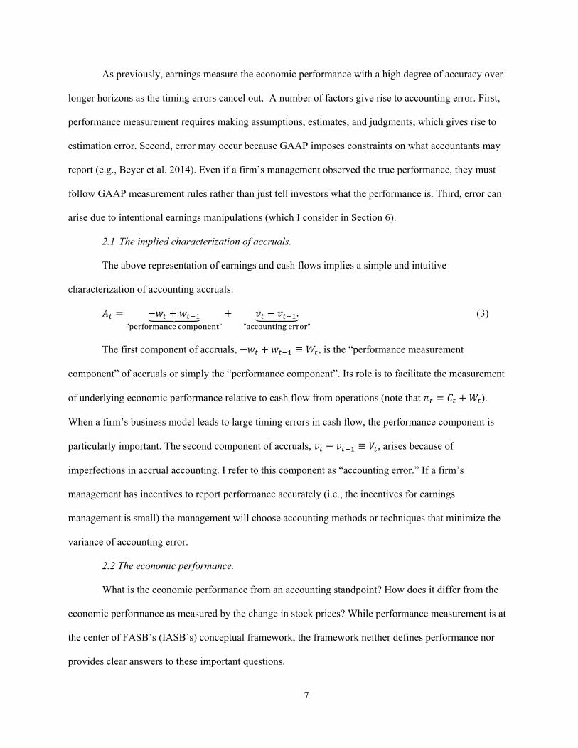
As previously, earnings measure the economic performance with a high degree of accuracy over
longer horizons as the timing errors cancel out. A number of factors give rise to accounting error. First,
performance measurement requires making assumptions, estimates, and judgments, which gives rise to
estimation error. Second, error may occur because GAAP imposes constraints on what accountants may
report (e.g., Beyer et al. 2014). Even if a firm’s management observed the true performance, they must
follow GAAP measurement rules rather than just tell investors what the performance is. Third, error can
arise due to intentional earnings manipulations (which I consider in Section 6).
2.1 The implied characterization of accruals.
The above representation of earnings and cash flows implies a simple and intuitive
characterization of accounting accruals:
” ”
.” ”
(3)
The first component of accruals, ≡ , is the “performance measurement
component” of accruals or simply the “performance component”. Its role is to facilitate the measurement
of underlying economic performance relative to cash flow from operations (note that ).
When a firm’s business model leads to large timing errors in cash flow, the performance component is
particularly important. The second component of accruals, ≡ , arises because of
imperfections in accrual accounting. I refer to this component as “accounting error.” If a firm’s
management has incentives to report performance accurately (i.e., the incentives for earnings
management is small) the management will choose accounting methods or techniques that minimize the
variance of accounting error.
2.2 The economic performance.
What is the economic performance from an accounting standpoint? How does it differ from the
economic performance as measured by the change in stock prices? While performance measurement is at
the center of FASB’s (IASB’s) conceptual framework, the framework neither defines performance nor
provides clear answers to these important questions.

8
I define economic performance as the expected cash consequences of transactions or events
that took place in period (including the realized portion), provided that such transactions are subject to
accounting measurement. Analytically, performance is defined as follows:
| , (4)
where ∑ , is the sum of cash flows from all anticipated individual cash-generating
transactions taking place at time 1. Operator excludes future cash flows not subject to accounting
measurement at time . Specifically, ∑ , , is the sum of cash flows over all possible cash-
generating transactions taking place at time 1 multiplied by , 0,1 , which takes the value of
one when transaction is subject to measurement (recognition) under GAAP at time (typically as a
result of another transaction or event, e.g., delivery). Thus, unrealized performance in equation (4)
represents expected future cash flows subject to accounting measurement as of the end of period (e.g.,
net receivables). In contrast, the realized portion consists of (i) unexpected shocks to cash flows
anticipated and included in the prior period’s performance, | and (ii) cash
flows realized at time that were not subject to recognition at 1, 1 . Substituting
these terms into equation (4), we can express performance as:
| | . (5)
Performance thus can be expressed as cash flow less its expected portion included in ,
plus the expected cash flows from transactions in period 1. When | is positive (negative),
it represents the accrued (deferred) portion of performance, i.e., an asset (liability) on the balance sheet.
This clarifies that conceptually the timing error is an inverse of future expected cash flows:
| . Timing error, in a classic sense, is a shock to cash flow, , unrelated to current
performance: 1 and 0, e.g., as a result of investment (purchases of assets that will be
used in future periods) or taking credit (liability). For example, a purchase of inventory reduces and
increases | by the same amount. Postponing a payment to suppliers or employees increases

9
but reduces | . Timing errors thus introduce a strong correlation between and and not
between and . This implies that cash flows are more volatile than performance (if the opposite was
true, the variance of would exceed the variance of ). On the surface, it seems that economic
performance is subject to the timing error in the same way cash flow is. However, this is not the case, as
can be seen from the equation (4) given that cash flow shocks and are orthogonal (the implication
is that the true performance is sustainable).
An analogy can be made between accounting performance and market performance, which can be
defined as (inclusive of any dividends):
… | … | , (6)
where cash flows are discounted and information set is all information reflected in stock prices as of
time . This is analogous to a more general definition of accounting performance:
| | , (7)
where ∑ , , ∑ , , , and , 0,1 depending on whether an anticipated
future transaction, , is measured under GAAP at time .4 Future cash flows may or may not be
discounted under GAAP, depending on the accounting treatment (the accounting performance is defined
accordingly).
Thus, conceptual similarities exist between market performance and accounting performance.
However, there are also two key distinctions. First, accountants do not measure all cash flow
consequences of current economic transactions or events. For example, given that the distant cash flows
associated with delivering goods and services, , are uncertain, 0. If this happens for cash
flows with 1, equation (7) reduces to equation (5). For the case of working capital accruals that
estimate to cash flows within one year, 1.
Second, the information set that accountants have, , is different from the information set, ,
reflected by the stock price. Accountants do not observe all information that is impounded in stock prices.
4 Performance thus is a part of Hicksian income (Hicks 1946), i.e., excluding a portion of such income that is not subject to accounting measurement (e.g., changes in future prospects or growth opportunities).

10
At the same time, they have performance relevant information that market obtains from (the release of)
financial statements. The latter is something that makes accrual accounting valuable to investors. It is
important to note that accounting performance, , is defined with respect to the information set available
to accountants, , as opposed to being defined in some absolute sense or with respect to an arbitrary
information set. To the extent that accountants do not observe some information (which is always the case
in real life), the measurement and recognition of its cash consequences are deferred until this information
comes out (e.g., realization happens). In other words, hidden information is viewed as performance only
when it is discovered and becomes available to accountants.
2.3 Accounting error.
Accounting error arises from the difficulties associated with measuring (estimating) the expected
future cash flows, , given the information set available to accountants. Specifically, if ∗ as an
estimate of | , accounting error is defined as the difference between estimated and expected
cash flows:
∗ | | . (8)
This definition of accounting error is in line with SFAC 7, which discusses the distinction
between estimated and expected cash flows (expected cash flow is the sum of probability weighted
amounts in a range of possible estimates).
The estimation is unbiased when we have the following property:
| ∗ | | 0. (9)
2.4 Extended numerical example.
The model given by equations (1)-(4) captures the salient properties of accrual accounting. Let
me illustrate this with an intuitive example. Suppose a company generates $1,000 worth of sales in period
and collects $900 cash. Suppose the true probability of collection equal 95% while an accountant
estimates the probability to be 96%. What are the economic performance, timing, and accounting errors in
this case? The economic performance is: 900 100 ∗ 0.95 $995. The timing error is

11
accordingly: E collections 0.95 ∗ 100 $95, and the corresponding “perfect
accrual” is $95. Finally, the accounting error is E collections E collections
96 95 $1.
This has two implications for what happens in period 1. First, the reversal of the $1
accounting error will take place in period 1, when collections occur. If the actual amount collected in
period 1 is in fact $95, a $1 write-off corrects the $1 overstatement. The actual collection of
receivables, however, does not have to equal $95, which is the expected value. If the actual collections
were $92 ($98) instead, the unexpected cash flow shock is $3 ( $3 . This wedge between realized
and expected cash flows is not a part of accounting error but a consequence of new information unknown
at time . Since it was impossible to anticipate at time , and since it is both earned and realized at time
1, it is a part of . What matters most here is that the higher the overstatement of performance at
time , the lower the earnings at time 1. In contrast, true performance does not feature such reversal
patterns.
2.5 Understanding accounting quality.
Consistent with the Statement of Financial Accounting Concepts No. 8 (see also SFAC 1), I
define the quality of accounting earnings (accruals) in the following way: accounting quality is the extent
to which accrual accounting reflects the unobservable economic performance. The three components
responsible for the quality of accounting earnings and accruals are: the variability of economic
performance, ; the variability of the performance component, ; and the
magnitude of accounting error, . The first component, , the variance of the economic
performance, reflects uncertainty about the future or the riskiness of the business a company. Variance of
the performance component , the signal in accruals, reflects operating volatility, i.e., liquidity shocks to
which a firm’s business model is subject. The value added by accrual accounting increases in and this
component can hence be thought of as the benefit of using accruals. The performance component is of
particular importance to understanding the demand for accrual accounting. Finally, reflects the

12
noisiness of accruals and earnings and thus represents a cost of accrual accounting.
While these three variance components are interesting in their own right, one can also evaluate
accruals quality in terms of their signal-to-noise ratio, / , or its bounded counterpart:
AccountingQualityRatio ≡ ,
which is analogous to R2, showing the fraction of accruals’ variance explained by the performance
component. The numerator captures the signal contained in accruals (i.e., the benefit side), which is
scaled by the magnitude of the noise in accruals (the cost side). It is important to note that this ratio does
not capture all the aspects that characterize accounting quality. Depending on the research objective, the
variance of the accounting error or the variance of the performance component (or their correlation) may
be of interest. Additionally, one can quantify the quality of earnings and cash flows in terms of the
following signal-to-noise ratios:
r / E ≡ EarningsQuality, and r / C ≡ .
2.6 Distinctions from prior models of accruals.
The proposed model of accruals differs from those used in prior studies (e.g., Healy 1985, Jones
1991, Dechow, Kothari, and Watts 1998, Dechow and Dichev 2002). The most notable distinction is that
the model does not decompose accruals into discretionary and non-discretionary components (Healy 1985
and DeAngelo 1986). Conceptually, discretionary accruals aim to measure economic performance (but
may also contain manipulations) given that accounting discretion is granted to a firm’s management to
allow those with a better understanding of the firm’s economics to measure performance more accurately
(e.g., Watts and Zimmerman 1990). At the same time, both and components have discretionary and
non-discretionary parts. For example, may arise because management uses accounting discretion to
achieve a performance target or it makes a discretionary error when estimating, e.g., a bad debt expense.
At the same time, may also arise because a manager does not have full discretion over the reported
numbers under GAAP.

13
My model is also conceptually different from that in Dechow and Dichev (2002) (I provide a
detailed discussion in Appendix A). The central distinction is in the accounting error construct, namely,
whether it is an ex post vs. ex ante construct. In the Dechow and Dichev (2002) model, the accounting
error arises from the need to estimate cash flows unknown at time . This is done by accruing an
amount E . They define accounting (estimation) error as follows (see Dechow and Dichev [2002,
38]):
E E E :
E
:
. (10)
As the equation indicates, this error can be decomposed into two mutually uncorrelated
components. The first component is the difference between estimated and expected cash flow, which
reflects accounting. The second, , is driven by the arrival of new information or due to the occurrence
of economic events during the period 1. It is not a result of accounting error and in fact is outside the
accountants’ control. It represents a shock to future cash flows that could not be expected at time and
one should think of as a portion of 1 performance, rather than an error accountants make. Thus,
conceptually, the error in the Dechow-Dichev model does not separate the (ex ante) accounting error from
the ex post performance.5
2.7 Reconciling different views on accounting quality.
Dechow et al. (2010), among others, argue that accounting quality is viewed differently by
different users of accounting information (e.g., debtholders vs. shareholders). This view does not
contradict the view in this paper. Irrespective of who uses the accounting information, the decision maker
is ultimately interested in understanding the economic performance, , and separating it from accounting
noise. However, different users of accounting information may disagree about the measurement and, as a
5 To appreciate this distinction more fully, consider mark-to-market accounting for marketable securities. At any point in time t, liquid markets guarantee prices that measure future expected cash flows from the sale of these securities with a very high degree of accuracy. Thus, ex ante, we know that accounting quality is very high. However, the actual future cash flows realized at time t+1 from the sale of these securities can be very different given that prices can move considerably in response to new information. Such ex post movement is not a part of accounting error in my model.

14
result, the properties of accounting error. In particular, different users place different weights on
information qualities, such as neutrality, conservatism, relevance, reliability, and consistency, all of which
can have an effect on . The question thus becomes: what are the desirable properties of accounting error
? This question is of primary importance in the accounting literature. In a statistical sense, we would
like to resemble white noise that has low variance and is self-corrected (i.e., reverses) over time. In a
world with frictions, e.g., earnings management, such an outcome may or may not be attainable and hence
the properties of accounting error are shaped by the demands from different parties and involve tradeoffs
(e.g., relevance vs. reliability).6 As I discuss further, the approach I offer can be used to study the
properties of accounting error (e.g., conservatism, or correlation with performance), and thus can prove
instrumental to understanding the economic tradeoffs related to accounting measurement.
3. Identification of Accounting Quality.
The key question in the accounting literature on earnings quality is how to separate the
underlying economics, i.e., the portion of accruals that captures economic performance from that which
reflects the error in measuring such performance. This challenging task requires explicit consideration of
the identifying assumptions. The central idea of this paper is that the institutional properties of accounting
processes, namely that (1) cash flows and earnings share the same performance components and (2) the
accounting error in accruals and the performance component reverse over time, serve as a “hook” to tease
out the economic performance in accruals and separate it from accounting error. These properties are
embedded into the model given by equations (1)-(3) above and shape the moment conditions among
accounting time series. It is necessary to make additional statistical assumptions that capture the statistical
properties of both accounting error and performance. The identification of accounting quality is feasible
under different sets of assumptions, as I will discuss throughout the paper.
3.1. Regression-based approach.
6 While some users would prefer a measurement system that is immune to manipulations (e.g., when writing accounting covenants) and hence emphasize reliability, others may look past earnings management when discovering a stock price and could thus emphasize the relevance dimension of accounting information (e.g., fair value measurement).

15
To begin the discussion of identification issues, it is useful to consider a regression-based
approach to earnings quality. If one had a set of determinants that fully explained the performance portion
of accruals, , the identification of accounting error in accruals would be
straightforward. One could effectively control for by using these determinants in a linear regression
and take the variance of the residual from this regression as a measure of accounting error. This is the lens
through which prior measures can be viewed. The two primary methodologies for measuring the quality
of accruals (the seminal contributions of Jones (1991) and Dechow and Dichev (2002) as well as a
number of their variations), use linear regressions to control for the “normal” or non-discretionary portion
of accruals. The variance of the residuals from these models (i.e., abnormal or discretionary accruals) are
used as measures of accruals (earnings) quality (e.g., Francis et al. 2004).
The first thing to note about the regression approach is that it requires identifying assumptions.
Even if one could effectively control for the performance portion of , running an OLS regression
implicitly assumes that that all the determinants of and are uncorrelated. A more fundamental issue,
however, is that this approach, in principle, cannot fully control for using observable variables. If one
could control for with a high degree of accuracy, one would be able to provide a better solution to the
problem (performance measurement) that GAAP is trying to solve using accruals. This contradicts the
logic of having GAAP in the first place. As a result, the regression approach cannot fully isolate the
performance component of accruals to obtain an estimate of accounting error irrespective of the
identifying assumptions one is willing to make. Consistent with this argument, a number of studies
express a concern that measures of accounting quality do not isolate the economic performance present in
accruals (e.g., Dechow, Ge, and Schrand 2010, Wysocki 2009). See Appendix A for additional
discussion.
3.2. Identification strategy and assumptions
My identification strategy relies on the model given by equations (1)–(3) to tease out the
parameters of interest. I propose using moment conditions of the accounting time series: earnings, cash

16
flows, and/or accruals, in combination with the model given by equations (1)–(3) as a basis for
identification of the accounting quality parameters. For example, if accountants make a measurement
error (random or intentional) by overstating receivables in the current period, all else equal, the future
earnings are expected to be lower by the same amount. At the same time, true performance should not
exhibit reversal. These properties allow for statistical discrimination between performance and accounting
error.
It is also necessary, however, to make additional statistical assumptions about the unobservables,
, , and , in order to estimate their variances. While the model can be estimated under different sets
of statistical assumptions, I begin by discussing a benchmark case that serves as a basis for more
complicated models. Subsequently, I discuss how some assumptions can be relaxed or avoided to
improve model specification.
The benchmark case is motivated by what may be thought of as a “frictionless” measurement
system. In such a system, accounting error should resemble white noise, uncorrelated with the economic
performance or the timing error in cash flows. Accordingly, I make the following baseline assumptions:
Assumption A. The process has a finite variance and is uncorrelated with errors and .
Assumption B. The vector of errors , is a white noise vector (independent and serially
uncorrelated variables with finite variance).
Zero correlation between and (and and ) follows from the assumption of unbiased
estimation, E | 0. The idea is that if accountants systematically over- or under-accrued when
accounting for performance fluctuations (i.e., a positive (negative) correlation between economic
performance and accounting error), then it would be possible to adjust the estimation technique in a way
that reduces accounting error. Recall that | and
| , i.e., they only depend on information known by the end of time . This
implies that the unconditional moments 0. This follows from the law of
17
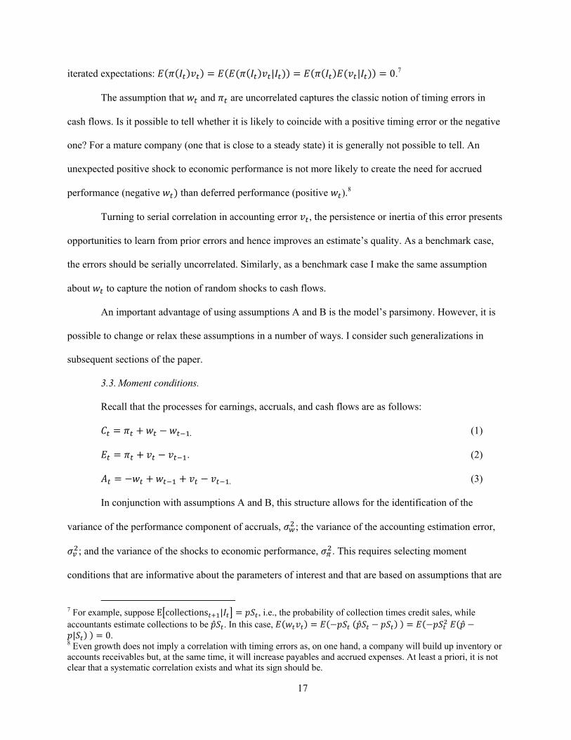
iterated expectations: | | 0.7
The assumption that and are uncorrelated captures the classic notion of timing errors in
cash flows. Is it possible to tell whether it is likely to coincide with a positive timing error or the negative
one? For a mature company (one that is close to a steady state) it is generally not possible to tell. An
unexpected positive shock to economic performance is not more likely to create the need for accrued
performance (negative than deferred performance (positive ).8
Turning to serial correlation in accounting error , the persistence or inertia of this error presents
opportunities to learn from prior errors and hence improves an estimate’s quality. As a benchmark case,
the errors should be serially uncorrelated. Similarly, as a benchmark case I make the same assumption
about to capture the notion of random shocks to cash flows.
An important advantage of using assumptions A and B is the model’s parsimony. However, it is
possible to change or relax these assumptions in a number of ways. I consider such generalizations in
subsequent sections of the paper.
3.3. Moment conditions.
Recall that the processes for earnings, accruals, and cash flows are as follows:
. (1)
. (2)
. (3)
In conjunction with assumptions A and B, this structure allows for the identification of the
variance of the performance component of accruals, ; the variance of the accounting estimation error,
; and the variance of the shocks to economic performance, . This requires selecting moment
conditions that are informative about the parameters of interest and that are based on assumptions that are
7 For example, suppose E collections | , i.e., the probability of collection times credit sales, while accountants estimate collections to be ̂ . In this case, ̂ ̂| 0.
8 Even growth does not imply a correlation with timing errors as, on one hand, a company will build up inventory or accounts receivables but, at the same time, it will increase payables and accrued expenses. At least a priori, it is not clear that a systematic correlation exists and what its sign should be.

18
likely to be descriptive (Andrews and Lu 2001). The choice of moments is not guided by econometric
theory and is more an art than a science. In general, moments should be chosen to provide substantial
information about the parameters of interest, i.e., changing a parameter should have a first-order effect on
the moment (thus, for example, moments based on distant lags, , are unlikely to be useful as they
are close to zero). Additionally, moments that rely on assumptions that are unlikely to be met should be
avoided. Finally, moments that are linearly dependent will not add information (e.g., moment E
does not add information if moments E and E are used).
The following set of moment conditions suffices to identify the parameters of interest under the
baseline assumptions, although other moments can be used as well (for example, the moment E
can also be useful). Note that all variables are measured as deviations from their means.
1 : E 2 ,
2 : E 2 ,
3 : E 2 2 ,
4 : E ,
5 : E ,
6 : E ,
where is the first-order auto-correlation of economic performance , i.e., the persistence of the
underlying economic performance.9 These moment conditions present six equations with four unknowns.
The first three equations facilitate identification by exploiting the information in two different
performance measures, whereas the last three moments also exploit the reversal in the error components.
GMM estimation can be used to identify and consistently estimate the parameters , , , and at
the firm or industry level.10
As an alternative set of moments, one can use changes in the time series of earnings, cash flows,
and accruals. In this case, it is important to account for differences in the dynamics of the three time
9 Note that the moment conditions are still meaningful even if the parameters change over time. Suppose ,
| , which is a conditional expectation based on information, e.g., some type of economic shock, at time . In this case, ≡ | , , where the first equality follows from the law of iterated expectations. In other words, moments should be interpreted in terms of the unconditional (average) variance of, for example, accounting error and other variables. One could also consider modelling , as a function of time and firm characteristics. 10 Maximum likelihood can also be used to estimate these parameters. Doing so generally increases the efficiency of the estimates but requires distributional assumptions such as normality.

19
series. For example, the differenced version of the accrual process given by equation (3) is as follows:
2 2 . (11)
The differenced formulation implies the following set of moment conditions:
1’ : E ∆ ∆ ∆ 6 ,
2’ : E ∆ ∆ ∆ 6 ,
3’ : E ∆ ∆ 6 6 ,
4’ : E ∆ ∆ ∆ ∆ 4 ,
5’ : E ∆ ∆ ∆ ∆ 4 ,
6’ : E ∆ ∆ 4 4 ,
where ∆ is the first-order auto-correlation of changes in the economic performance, ∆ .
This set of moments is more robust to certain types of misspecification. First, the process may be non-
stationary (e.g., a random walk), in which case the variance of increases without a bound (i.e.,
assumption A is violated, which means that the parameters cannot be estimated consistently). However,
process ∆ is more likely to be stationary. Second, differencing effectively eliminates a persistent
component of accruals due to, for example, growth or the presence of long-term accruals, such as
depreciation, amortization, and deferred taxes, which is a potential source of misspecification in an
empirical implementation.
3.4 Generalized versions of the model.
In the remainder of this section, I discuss how the baseline assumptions can relaxed or avoided.
For example, the timing error, , may be auto-correlated and/or exhibit some correlation with
performance due to growth. Accounting error may be correlated with timing error (this may be a
consequence of accounting conservatism, as discussed in Section 6). Finally, the underlying economic
performance may be correlated with accounting error due to earnings management (Healy 1985,
McNichols and Wilson 1988, Gerakos and Kovrijnykh 2013). In this and subsequent sections of the
paper, I consider scenarios that allow for these possibilities.
Several directions to generalize the model deserve consideration and involve different tradeoffs.
For example, relaxing assumptions by increasing the number of parameters can improve the fit but also
lower the loss of reliability in the estimates (particularly when the time series are short). With this in
20
mind, several directions deserve consideration.
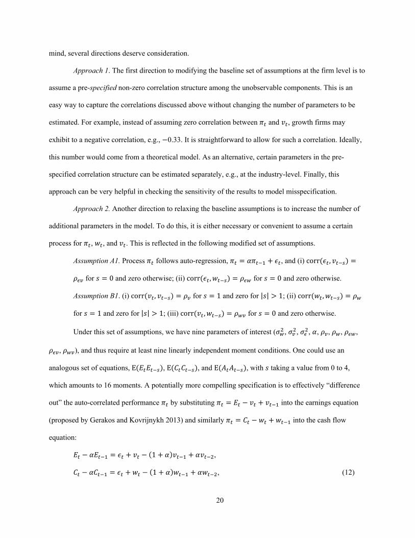
Approach 1. The first direction to modifying the baseline set of assumptions at the firm level is to
assume a pre-specified non-zero correlation structure among the unobservable components. This is an
easy way to capture the correlations discussed above without changing the number of parameters to be
estimated. For example, instead of assuming zero correlation between and , growth firms may
exhibit to a negative correlation, e.g., 0.33. It is straightforward to allow for such a correlation. Ideally,
this number would come from a theoretical model. As an alternative, certain parameters in the pre-
specified correlation structure can be estimated separately, e.g., at the industry-level. Finally, this
approach can be very helpful in checking the sensitivity of the results to model misspecification.
Approach 2. Another direction to relaxing the baseline assumptions is to increase the number of
additional parameters in the model. To do this, it is either necessary or convenient to assume a certain
process for , , and . This is reflected in the following modified set of assumptions.
Assumption A1. Process follows auto-regression, , and (i) corr ,
for 0 and zero otherwise; (ii) corr , for 0 and zero otherwise.
Assumption B1. (i) corr , for 1 and zero for | | 1; (ii) corr ,
for 1 and zero for | | 1; (iii) corr , for 0 and zero otherwise.
Under this set of assumptions, we have nine parameters of interest ( , , , , , , ,
, ), and thus require at least nine linearly independent moment conditions. One could use an
analogous set of equations, E , E , and E , with taking a value from 0 to 4,
which amounts to 16 moments. A potentially more compelling specification is to effectively “difference
out” the auto-correlated performance by substituting into the earnings equation
(proposed by Gerakos and Kovrijnykh 2013) and similarly into the cash flow
equation:
1 ,
1 , (12)

21
.
There are a number of ways that these equations can be used to formulate moments (note that the
last equation is no longer a linear combination of the other two equations). One convenient possibility is
to use moments of the form:
E )( 2 2 1 2 1 .
I provide the complete set of moments, up to three lags, in Appendix C.1. Another possibility is
to multiply both sides of the first equation by (second equation by ), which is analogous to the
Yule-Walker equations. An obvious limitation of this brute force approach is that it adds considerably
more parameters (and algebraic complexity), which is problematic when the time series are short.
Approach 3. The third direction involves altering the baseline assumptions to specify a
parsimonious alternative. For example, one can allow for auto-correlation in the timing errors as well
as for their correlation with performance by assuming that the timing error in cash flow has the form
, such that:
. (13)
This structure of accruals may be descriptive for some business models and preserves the number
of parameters to be estimated.
Approach 4. Finally, a promising way to preserve model parsimony is to incorporate possible
growth via firm characteristics. In particular, to accommodate a possible persistence in the timing error
and simultaneously allow for its correlation with performance, the timing error can be modeled as a
function of firm characteristics correlated with performance (but uncorrelated with accounting error, i.e.,
instruments), such as firm size, market capitalization, growth in fixed asset base, and stock performance.
Specifically, let’s define cash flow ∗ ∗ and ∗ . The systematic
component, , is correlated with performance and autocorrelated over time, whereas is an
orthogonal non-systematic component. In this case, the model can be written as:
.

22
∗ Δ . (14)
∗ Δ .
Knowledge of allows adjusting accruals and cash flows in a way that accommodates the
presence of the systematic performance component (which may be correlated with performance or over
time in any arbitrary manner) effectively eliminating its effect. In such a case, the baseline assumptions A
and B, with respect to , , and , are less likely to be violated. Note that can be identified
separately (or simultaneously) based on the following moment conditions:
∆ ∆ ∆ 0. (15)
Given that ∆ 0 by assumption.
In sum, there are a number of directions for relaxing the baseline assumptions and addressing
potential misspecifications. These offer a number of opportunities for future research.
4. Empirical Implementation
The primary objective of this paper is conceptual: it offers a new approach to modelling accruals
and measuring accounting quality. Uncovering model specifications that have the best fit with the data,
which can vary by industry or even firm, is a non-trivial task that lies outside the scope of this study. To
demonstrate that the proposed approach has a straightforward implementation and that it generates
plausible results, I estimate three parsimonious model specifications. First, I estimate a “levels”
specification based on moments (1-6), described in Section 3.2. Second, I estimate a “changes”
specification based on moments (1'-6'), described in the same subsection. This specification addresses
possible non-stationarities in performance via differencing. Third, I use generalized specification based on
Approach 4, outlined in Section 3.3. This specification relaxes baseline assumptions by allowing for a
systematic component of the timing error, potentially correlated with performance. The set of
instrumental variables ∆ consists of changes in the log of market capitalization (∆log ), changes in
the log of non-current assets (∆log ), and changes in the ratio of market value of assets to book value

23
of assets (∆ / ). These variables are assumed not to exhibit correlations with accounting error. Both the
second and third specifications aim to accommodate variations of firm growth in the time series.
The primary empirical questions of interest are: Does the performance component in accruals
exceed the amount of accounting noise? What fraction of variance in accruals is explained by the
performance component? The answers to these questions are fundamental to the economic justification
for the use of accruals. I also explore whether the variance components , , and are economically
different or whether they vary in the same way with a set of common determinants. Finally, I explore
whether these parameters are differentially priced by the auditors.
I use data from Compustat for the period from 1987 to 2015 to address this question and also to
conduct several other types of analysis. I conduct the analysis at the industry level and then at the firm
level. To estimate the firm-level parameters, I require 15 or more observations per firm with non-missing
values for accounting variables. I defer details on sample construction and variable measurement to
Appendix B. The resulting sample consists of approximately 2,200 firms, spanning 39 industries. Table 1
provides the summary statistics for the variables used in the estimation and subsequent analysis.
4.1 Does the performance component of accruals dominate accounting noise?
Table 2 presents parameters of interest estimated by industry using GMM. Panels A-C present the
estimates based on the “levels”, “changes”, and “generalized” model specifications, respectively. Panel A
indicates that the average (median) standard deviation of economic performance, , is 0.055 (0.053).
This is the largest parameter in terms of economic magnitude. It is followed by the average (median)
standard deviation of the performance component of accruals, , which is equal to 0.026 (0.025). The
average (median) standard deviation of the accounting error, , is 0.018 (0.017). Panels B and C show
similar and even somewhat more pronounced results. For the “changes” specification, the parameters
and are 0.024 and 0.013, respectively, whereas for the generalized model they are 0.026 and 0.015,
respectively. In all three cases, the differences are positive and highly statistically significant.
The results in this panel contrast substantially with the explanatory power based on traditional

24
regression models. The performance component of accruals explains a much greater fraction of accruals
variance as compared to the variance explained by the regression models. In particular, the average
(median) accounting quality ratio, / , ranges between 0.68 (0.67) and 0.75 (0.76). In contrast,
Panel D indicates that the R2 based on the Jones (1991) or Dechow and Dichev (2002) models are on
average (median) 0.07 (0.07) and 0.35 (0.35). These results confirm that the residual variation in these
models measure (conceptually) different constructs. My findings in Table 2 are more in line with Beyer et
al. (2014), who use equilibrium conditions to derive industry-level estimates of accounting noise present
in the book values of equity. They find that the ratio of the variance of accounting noise to that of
economic performance is roughly 50%. While the parameters are not directly comparable (due to scaling
and given that they do not use accruals or cash flows), this is broadly consistent with my findings that
accounting error is under 50% of the variance of economic performance.
Table 3 presents the analogous set of results estimated by firm. As previously, the “levels”,
“changes,” and the generalized specifications are reported in Panels A-C, respectively. The results at the
firm level are similar to the industry-level findings. Panel A indicates that the average (median) standard
deviation of economic performance, , is 0.051 (0.044). It is followed by the average (median) standard
deviation of performance component, = 0.022 (0.020), and subsequently by the accounting error
component, = 0.015 (0.012). The magnitudes of the average (median) performance and accounting
error components in Panel B are = 0.021 (0.018) and = 0.011 (0.009), respectively. Panel C indicates
that = 0.020 (0.018) vs. = 0.011 (0.009). All these differences are highly significant. The mean
(median) accounting quality ratio, / , ranges between 0.65 (0.71) to 0.71 (0.79), which
continues to contrast markedly with the average explanatory power of the regression-based models in
Panel D.
The evidence in Tables 2 and 3 confirms that, across three model specifications estimated both at
the industry and firm levels, the magnitude of the performance component in accruals dominates the
accounting error component. This constitutes evidence that accrual accounting improves performance

25
measurement compared to cash flow-based measures, in line with SFAS 1 and 8. My results support the
notion that for users of financial statements, the benefits of accrual accounting outweigh the costs.
4.2 Does accounting error share much common variation with performance?
The question that arises next is whether the variance components, , , and , share much
common variation cross-sectionally, i.e., are they driven by the same set of the factors? I investigate this
question in Tables 4 and 5 by examining their cross-sectional determinants. Table 4 presents the results
from the following cross-sectional regression based on parameters from the three previously identified
model specifications:
, , , , (16)
where is a firm subscript.
The results indicate that both , and , exhibit positive and highly significant associations
with , across the “levels”, “changes”, and generalized specifications. Such results are intuitive, as
greater uncertainty about economic performance or timing error is likely to be associated with the
presence of errors when measuring performance. However, when included individually, , explains
only 6-10% of the variation in , , depending on model specification. Jointly, , and , explain up to
22% of the cross-sectional variation in , . Overall, it does not appear that the three parameters are driven
by the set of a few common factors.
4.3 Determinants of variance components σ , σ , and σ .
Table 5 explores economic determinants of the three variance components: , , and , based
on the following cross-sectional regression:
, (17)
where is one of the three variance components and is a vector of firm-
characteristics. The firm characteristics I examine include size (Size); number of employees (Employees);
uncertainty (Uncertainty); book-to-market ratio (B/M); leverage (Leverage); profitability (ROA); liquidity
(Liquidity); operating cycle proxies, namely, days in accounts receivable (Days receivables) and

26
inventory (Days inventory); as well as the length of the fixed assets life cycle (Asset life). These variables
are averaged over the same period over which the parameters of interest are estimated.
The table indicates a number of significant associations between each variance component and its
determinants. The coefficient estimates are overall consistent across the three model specifications. In
many instances the results are intuitive. Size is negatively associated with both accounting error and the
timing error (and with performance when Employees is omitted). As one would expect, higher
Uncertainty is associated with greater values for all three parameters, , , and . In contrast, higher
Leverage or longer Asset life are associated with lower values for the parameters. Interestingly, the
remaining explanatory variables do not exhibit associations of the same sign across , , and . As
one would expect, the operating cycle (Days receivables and Days inventory) exhibits a positive link with
accounting error. At the same time, it is negatively associated with the variance of economic performance.
Employees is associated with a lower variance of economic performance but not accounting or timing
errors. B/M, and Profitability exhibit a negative association with accounting error but are positively
related to the timing error. While understanding the explanations behind these associations more fully is
outside the scope of this paper, the main takeaway from this analysis is that the three variance
components appear to be explained by different economic factors.
4.4 Is the accounting error vs. performance component priced differently by the auditor?
The last question I explore empirically is whether there are different pricing implications to
accounting error vs. timing error as far as auditors are concerned. While the auditors will generally not be
able to identify accounting (estimation) error and separate it from timing error, they should be able to tell
when such errors are more likely to be present. I hypothesize that auditors will price both accounting error
and timing error in accruals as both of these create the demand for accrual accounting and hence for an
audit. However, I further hypothesize that the accounting error will be priced at a higher rate because it
imposes additional risk on the auditor (e.g., Hribar, Karvet, and Wilson 2014). To test this hypothesis, I
run the following regression:
log ∑ , (18)

27
where the control variables include a broad set of firm characteristics known to be associated with audit
fees in prior studies (e.g., Simunic 1980, Hribar, Karvet, and Wilson 2014). Because it is not always clear
that it is necessary to control for certain firm characteristics, as they may be correlated with accounting
quality, I estimate the model with and without controls (except for Size, given the nature of the dependent
variable).
The results for this analysis are presented in Table 6. The analysis suggests that all three
components explaining the variance of cash flows and accruals are priced by the auditor. The component
with the lowest pricing multiple is the volatility of economic performance. It is followed by the volatility
of the performance component of accruals. In other words, the variance of high quality accruals is priced.
These results are consistent with the notion that unexpected changes in firm performance as well as the
presence of timing errors increase the demand for an audit. However, the evidence indicates that
accounting error has the highest audit pricing implications. A unit of variance of accounting error is
priced at approximately double what a unit of timing error is priced at and is over five times the pricing of
the variance of economic performance.
As a robustness check, I repeat this analysis using the ratio of audit fees to total assets as the
dependent variable. This analysis is reported in Table 7. While the magnitudes of the coefficients are
different, the inferences are largely unchanged. In fact, the results are even more pronounced, particularly
when the control variables are added (in which case the performance component becomes insignificant).
Overall, the results from this analysis are in line with the prediction that the variance of accruals
explained by accounting error vs. performance is priced differently. More generally, the analysis in this
section suggests that my approach to modelling accruals is straightforward to implement and that it
generates a number of new insights about accruals undocumented elsewhere.
5. Model Extensions
The model can be generalized in several ways to more explicitly capture certain properties of
accruals, such as conditional conservatism in earnings and one-time non-reversing items (disruptions to

28
accounting time series caused by significant events such as acquisitions or divestures (Hribar and Collins
2002)) or slow reversal patterns.
5.1 Incorporating accounting conservatism.
In this section, I discuss how the model can explicitly accommodate accounting conservatism – a
property of accrual accounting that has received much attention in the literature (e.g., Basu 1997, Chen,
Hemmer, and Zhang 2007, Ball and Shivakumar 2006, Nikolaev 2010, Gao 2013, Collins, Hribar, and
Tian 2014, among others).11 Ball and Shivakumar (2006) argue that accruals also accelerate recognition
of the unrealized economic losses and not gains that arise due to changes in expectations of future cash
flows. They argue that the inability to take this effect into account constitutes an important criticism of
discretionary accruals models. This view is consistent with accruals generating a better measure of
economic performance and unrealized gains and losses also being viewed as timing errors in cash flows.
The key issue here, however, is that the unrealized losses and gains follow an asymmetric treatment.
The approach offered in this paper can directly accommodate the asymmetric treatment of shocks
to economic performance. Given that the focus here is on the working capital accruals, let me start by
illustrating the intuition with an inventory impairment example, which follows the lower cost or market
rule. All else equal, consider a loss in inventory value of $100 that occurs in the present period
but is not realized until the next one, when the inventory is sold at a residual value. This loss implies a
timing error in cash flows $100 and requires a negative accrual of $100 to offset the
timing error. By analogy, an unrealized gain in the value of inventory $100 implies an equivalent
timing error in cash flows $100. Without a conservative treatment of gains, an accrual
$100 should be recorded. Because a conservative treatment of gains does not consider the $100 as current
income until the time of sale, it introduces a “conservative error” $100 into earnings (and
accruals). Not that such treatment can be an efficient way of offsetting managerial incentives to overstate
11 It is important to note that the presence of conservative accounting measurement need not lead to “conservative error.” Ideally, the effect of conservatism on earnings will precisely offset any positive bias a firm’s management may introduce, such that the resulting accounting error resembles white noise (and its reversal). See, e.g., Gao (2013). In practice, however, conservatism is likely to affect the properties of accruals and accounting error and in such cases, it should be possible to statistically detect it.

29
reported earnings and thus differs from estimation error more generally. One implication of the
asymmetric treatment of gains and losses is a non-linear correlation between and .
To allow for such properties in the accrual process, one can generalize the model in the following
way:
,
, (19)
c ,
where and represent the timing error in the absence of unrealized gains and losses, which follow an
asymmetric treatment (i.e., in the previously discussed sense). The component represents unrealized
gains (losses) that occur in the present period and is thus subject to asymmetric treatment. This
component is a part of economic performance but it falls out from the current cash flow due to its
timing error, . Because the conservative accounting treatment defers gains but recognizes losses, c
is expected to be zero for negative news, which is recognized in a timely manner, whereas it is expected
to be equal to in the case of unrealized gains that are deferred until realization.
Given the argument above, a natural candidate for the function c(.) is c max 0, .
Intuitively, when is negative, such as in the case of a decline in the value of inventory, the loss is
accrued in the same period, i.e., , whereas the corresponding part of accounting error, max 0, ,
is zero. In contrast, when is positive (as in the case of unrealized gain), conservative accounting
precludes recognition of , so that 0, whereas max 0, . The proposed way of
modelling asymmetric timeliness is equivalent to that in Ball, Kothari, and Nikolaev (2013).
Let’s assume that in the absence of unrealized gains and losses accompanied by conservative
accounting treatment, i.e., when the variance of is zero, the baseline assumptions A and B apply to the
components , , and , as previously. It is necessary to add statistical assumptions about to
formulate moment conditions:

30
Assumption C. The unrealized gain (loss) is uncorrelated with , , and and follows a
distribution symmetric around 0.
Under these assumptions, the following expectations will be satisfied:
E ,
E E max 0, g 0.5 ,
E E max 0, 0.5 ,
E E ,
E E max 0, 0.5 .
This structure relaxes the baseline assumptions we made earlier in a particular way allowing for
the asymmetric timeliness of unrealized gains and losses. The assumption of symmetry appears to be, at
least roughly, descriptive for many gains and losses (e.g., increases in cost of inventory seem to be as
likely, on average, as decreases).12 These expectations include an additional parameter, , and can be
straightforwardly integrated with the moment conditions discussed earlier. Doing so allows the estimation
and isolation of the portion of accruals explained by accounting conservatism, as well as the variances of
the remaining components of accruals.
5.2 Disruptions in accounting time series due to significant changes in the firm.
Hribar and Collins (2002) show that significant changes to a firm’s business, namely mergers and
acquisitions or divestures, introduce disruptions to the time series of accruals. While accruals from the
statement of cash flows can alleviate this issue, Owens, Wu and Zimmerman (2015) still find that
significant economic events such as mergers and discontinued operations inflate the proxies for
discretionary accruals. While issue applies to a lesser extent to working capital accruals, which are
typically used to measure accounting quality, it is useful to consider a way of addressing the presence of
disruptions in the accruals within the current framework.
12 One can also consider dropping the symmetry assumption by adding an extra parameter, . In this case, the following modifications occur: E E max 0, , E E max 0, , and E E max 0, .

31
The presence of a significant event does not always lead to a problem. For example, accruing a
large loss, e.g., due to litigation settlement, is a part of (an adverse shock to) current economic
performance. To the extent that we consider how to separate the current performance from accounting
error, this does not create a problem. This is different when an event introduces a one-time shock to
accruals or cash flows that is neither informative about the core operating performance nor should be
viewed as a part of accounting error, as would be the case for acquisitions or divestitures. Such
“disruptions” in the accruals time series can be modelled as a random variable whose sign and magnitude
depend on the nature of events as well as on other circumstances. Accordingly, let’s assume shock
affects accruals only in time periods when certain events take place. A possible disruption to cash flows
can be viewed in terms of a similar, possibly correlated, shock .
To accommodate such a scenario, the model can be modified in the following way:
,
, (20)
,
where ∈ 0,1 indicates whether an event takes place. The variables can be a result of mergers and
acquisitions, write-offs of non-current assets, discontinued operations, or special items and the associated
cash outlays. For simplicity, let’s assume that and are uncorrelated with other variables, such as
the core economic performance, and that the baseline assumptions apply. The variables and can
be correlated and can have non-zero means. In this case, the first three moment conditions (m(1)-m(3))
from Section 3.4 are modified as follows:
2 2 ,
2 ,
2 ,
where 1 . While these moments include more parameters, we now also can exploit an
additional set of moments:

32
E | 1 E | 0 ≡ ∆ ,
E | 1 E | 0 ≡ ∆ ,
E | 1 E | 0 ≡ ∆ ,
.
The quantities ∆ , ∆ , ∆ and can be computed separately and substituted back into the three
preceding moments for second stage.13 The GMM solution to these moments is a way to address the
presence of disruptions introduced into accruals by a significant event, such as mergers within the
proposed framework. What’s more, the number of parameters to be estimated remains effectively the
same as it was previously.
6. Modelling Earnings Management.
Up to this point, I have not considered how to discriminate between a “managed” (intentional)
component in accruals and a random error. In this section, I discuss several directions for accommodating
earnings management and how one can test for earnings management within the proposed framework.14
To allow for earnings management, one can break down accounting error as follows:
, (21)
where is a managed component of accounting error and is the portion of accounting error defined
as being orthogonal to the managed component. To separate the managed from the unmanaged
components, it is either necessary to exploit the incentives for earnings manipulations. These incentives
may arise from income smoothing considerations, as in Gerakos and Kovrijnykh (2013), or can be
captured by some external “partitioning” variables (e.g., Dechow, Sloan, and Sweeney 1995, Dechow and
Skinner 2000). I discuss these alternatives in the remainder of this section.
13 If one assumes that significant events affect accruals (cash flows) for two consecutive periods, one may further adjust the moments for quantities, E | 1 E | 0 ≡ ∆ ′, etc. 14 Dechow, Hutton, Kim, and Sloan (2012) and Gerakos and Kovrijnykh (2013) also exploit the reversal to estimate earnings management. Dechow et al. (2012) primarily use reversal as a way of gaining statistical power to detect earnings management rather than as an identification tool (identification comes from the specification of the exogenous partitioning variable); although they also argue that reversal improves the model specification. Gerakos and Kovrijnykh (2013) focus on the reversal of earnings management and do not model accruals or earnings quality more generally. These studies do not take advantage of the reversal of the performance component of accruals.

33
6.1 Modelling earnings management: Income smoothing.
Gerakos and Kovrijnykh (2013) argue that earnings management is manifested in earnings via
income smoothing (they do not model accruals and cash flows). They show that incentives to smooth out
shocks to economic performance arise under a fairly general set of managerial preferences.15 In line with
this intuition, they model earnings using the following dynamic structure:
, (22)
where true (unmanaged) economic performance, , follows an AR(1) process, . Based
on this assumption, earnings follow an ARMA process with a negative second-order auto-correlation of
the error term (see equation 12). They test for this auto-correlation of the error term and confirm their
predictions.16 Note that this model effectively assumes that the entire accounting error in accruals is due
to earnings management, i.e., 0 and . Otherwise, the model is not identified.
The approach offered in this study allows this assumption to be relaxed, such that the accounting error
includes both an unmanaged error and the income smoothing component:
. (23)
Assuming that baseline assumptions A and B are applicable under the null hypothesis of no
earnings management, i.e., when var 0 and , the following moments will be satisfied:
E , and E .
These expectations imply a straightforward modification to the moment conditions formulated
under baseline assumptions A and B and can be used to identify the parameters of interest. I defer the
details to Appendix C.2. The advantage of a moments-based estimation is that parameter can be
estimated directly as opposed to using the second-order auto-correlation of earnings residual suggested by
Gerakos and Kovrijnykh (2013). Additionally, this does not require the normality assumption necessary
for estimating the ARMA process.
15 Income smoothing is sometimes viewed as a way of eliminating noise in cash flows. The meaning I use is different: here, income smoothing results in earnings time series that exhibit a lower volatility compared to the volatility of the true underlying performance. 16 Estimation of the ARMA model requires distributional assumptions, namely, normality.

34
6.2 Directional tests of earnings management.
Another way to introduce earnings management is to rely on external information about
incentives to manage earnings (Dechow and Skinner 2000). Suppose we have a partitioning variable, ,
which is informative about managerial incentives to overstate (understate) earnings and accruals (i.e.,
estimation error). This could be a dummy variable for benchmark meeting or a variable indicating
proximity to a covenant violation. In this case, we can decompose accounting error as follows:
,
where is the managed component, , and captures the portion orthogonal to earnings
management.
To begin, let’s assume that is uncorrelated over time and uncorrelated with other variables in
the model (this would largely be the case for the dummy that a company just meets a benchmark and zero
otherwise).17. To avoid unnecessary parameters, I normalize to have a zero mean and unity variance.
As previously, let’s also assume that absent earnings management, the baseline assumptions A and B are
applicable. Under these assumptions, the following expectations hold:
E ,
E .
These expectations can be readily integrated with a set of moment conditions, e.g., those in Section 3.4
(see Appendix C.2. for a more detailed treatment). Note that one extra parameter and one extra moment
have been added, allowing this parameter to be identified. This approach allows decomposing accounting
error into managed and unmanaged portions. Simultaneously, the approach allows testing whether , and
hence earnings management, is statistically significant. Note that this model can be estimated using a
panel of firms or at the firm level.
6.3 Discussion
17 In reality, may be correlated with economic performance. Such a case is considered in Section 6.1, when
.

35
The approach to modelling earnings management proposed here is distinct from those in prior
studies that rely on discretionary accruals (e.g., Dechow, Sloan, and Sweeney 1995) and should be viewed
as complementary. One of the central issues in testing for earnings management is the need to isolate
economic performance in accruals (Kothari, Leone, and Wasley 2005). Kothari et al. (2005) rely on
performance matching to address this issue. However, performance matching cannot deal with the
earnings manipulations discussed in Section 6.1 (income smoothing) or instances where performance and
earnings management are correlated. I discuss this in more detail below.
Consider a case when the proxy for the incentive to manage earnings and the performance
component of accruals are correlated, such that:
, (24)
where is the portion orthogonal to . The source of correlation ( ) may be growth (McNichols
[2000, 2002]). I lay out the details of this model, including moment conditions, in Appendix C.3. To the
extent that discretionary accruals or performance matching do not fully isolate , the inferences about
earnings management will be confounded. To see this, suppose for simplicity that one uses total accruals
to test for earnings management by running the following regression: . The estimated slope
coefficient in this regression has the following expected value (recall 1 due to normalization):
E,
.
Depending on the sign of the coefficient of , the regression can over- or understate the
magnitude of earnings management, .
When is a dichotomous variable, this issue can be alleviated by using the performance
matching procedure in Kothari et al. (2005).18 Matching, however, is conceptually similar to a regression
18 When testing for earnings management, their study advocates controlling for performance in accruals by matching the treatment and control groups on current (or past) accounting performance (return on assets). The challenge faced by matching is that one cannot observe the true as opposed to the manipulated performance, which precludes a high quality match and hence full isolation of the performance component. Additionally, this approach in part matches on the dependent variable, as accruals are a significant part of the return on assets. This limits the hypotheses one can test, e.g., when earnings management itself is dependent on economic performance, as discussed in Kothari et al. (2005).

36
because it is carried out based on the reported (i.e., managed) performance, as opposed to the true
performance. In contrast, the modelling approach here offers an alternative by directly estimating .
This can be done by integrating the following two moments into the above framework:
E , and E .
The full set of moments can be found in Appendix C.3.19
In sum, the framework developed in this paper offers a way of testing for earnings management
that holds promise. To its advantage, it directly addresses the unobservable nature of economic
performance in accruals and requires explicit consideration of the assumptions under which the effect of
earnings management may be identified. It is important to note, however, this approach should not be
viewed as a substitute for other ways of testing for earnings management in the literature. It cannot
resolve all challenges by testing for earnings management and is also subject to misspecification.
Nevertheless, it offers a promising alternative and presents avenues for future research.
7. Conclusion.
I develop a new approach to modelling accounting accruals and provide an econometric strategy
to identify the quality of accruals and earnings. In line with the objectives of financial reporting, I model
accruals in a way that explicitly addresses their role in performance measurement (SFAC 8). Accruals
thus have two distinct components. The performance component reflects the portion of economic
performance not properly reflected in cash flows. The accounting error component takes place in the
process of measuring economic performance. The two components represent the benefit and cost of
accrual accounting, respectively. This characterization of accruals allows me to define accounting quality
in terms of a new construct: the degree to which accruals facilitate performance measurement, i.e.,
19 Another advantage to my approach over that of a regression-based framework arises when the incentive to manage earnings persists for several periods, e.g., , which is likely, for example, when accounting-based covenants are tight. Assuming, for the sake of illustration, that 0, we now have: E E
. In other words, the more persistent the earnings management is, the harder it is to detect within a regression framework, i.e., without accounting for persistence in . Intuitively, this difficulty arises because, due to reversals, it is harder to consistently overstate accruals for a number of periods in a row. In contrast, the following moment conditions make use of lags of to overcome this problem and identify the degree of earnings management, : E , and E .

37
capture the component missing from cash flows. In relative terms, accounting quality thus is the degree
to which the variance of accruals is explained by the performance component.
Besides offering a new model, I develop an econometric strategy to identify the quality of
accounting accruals and earnings under a flexible set of assumptions. The identification strategy revolves
around the institutional properties of accruals accounting. I use the notion that both cash flows and
earnings can be viewed as noisy measures of the same economic performance being measured and that
both the accounting error and the performance component of accruals reverse over time. These properties
serve as a “hook” that allows for discrimination between the performance and error component in
accruals under different sets of assumptions. The estimation relies on moment conditions based on
accounting time series, such as earnings, cash flows, and accruals. I implement several basic model
specifications and show that they generate a number of new insights. First and foremost, I show that the
performance component of accruals is significantly higher than the accounting error. This result is
important because it shows that accruals meet their objective of facilitating performance measurement.
I do not claim that the approach developed here is necessarily preferable to other measures of
accounting quality, which are based on different constructs (such as discretionary accruals). The choice of
construct generally depends on the research objective. One important advantage of my approach is that
allows most of the assumptions to be altered or relaxed. As such, the approach enables the search for a
better model and addresses possible specification issues that may arise in any particular application. I
discuss ways to relax key assumptions and extend the model to incorporate accounting conservatism and
earnings manipulations. The study offers a number of avenues for future research on accounting quality.

38
References
Andrews, Donald WK, and Biao Lu. “Consistent Model and Moment Selection Procedures for GMM Estimation with Application to Dynamic Panel Data Models.” Journal of Econometrics 101 (2001): 123-164.
Ball, Ray. “Accounting Informs Investors and Earnings Management is Rife: Two Questionable Beliefs.” Accounting Horizons 27 (2013): 847-853.
Ball, Ray, and Lakshmanan Shivakumar. “The Role of Accruals in Asymmetrically Timely Gain and Loss Recognition.” Journal of Accounting Research 44 (2006) 207-42.
Ball, Ray, S. P. Kothari, and Valeri V. Nikolaev. “Econometrics of the Basu asymmetric timeliness coefficient and accounting conservatism.” Journal of Accounting Research 51 (2013): 1071-1097.
Basu, Sudipta. “The Conservatism Principle and the Asymmetric Timeliness of Earnings.” Journal of Accounting and Economics 24 (1997) 3-37.
Beyer, Anne, Ilan Guttman, and Ivan Marinovic. “Earnings Management and Earnings Quality: Theory and Evidence.“ Stanford University working paper. (2014).
Chen, Qi, Thomas Hemmer, and Yun Zhang. “On the Relation between Conservatism in Accounting Standards and Incentives for Earnings Management.” Journal of Accounting Research 45 (2007): 541-565.
Collins, Daniel W., Paul Hribar, and Xiaoli Shaolee Tian. “Cash Flow Asymmetry: Causes and Implications for Conditional Conservatism Research.” Journal of Accounting and Economics 58 (2014): 173-200.
DeAngelo, Linda Elizabeth. “Accounting Numbers as Market Valuation Substitutes: A Study of Management Buyouts of Public Stockholders.” Accounting Review 61 (1986) 400-420.
Dechow, Patricia M. “Accounting Earnings and Cash Flows as Measures of Firm Performance: The Role of Accounting Accruals.” Journal of Accounting and Economics 18 (1994) 3-42.
Dechow, Patricia M., and Ilia D. Dichev. “The Quality of Accruals and Earnings: The Role of Accrual Estimation Errors.” The Accounting Review 77 (2002) 35–59.
Dechow, Patricia M., Weili Ge, and Catherine Schrand. “Understanding Earnings Quality: A Review of the Proxies, their Determinants and their Consequences.” Journal of Accounting and Economics 50 (2010) 344–401.
Dechow, Patricia M., Amy P. Hutton, Jung Hoon Kim, and Richard G. Sloan. “Detecting Earnings Management: A New Approach.” Journal of Accounting Research 50 (2012) 275-334.
Dechow, Patricia M., S. P. Kothari, and Ross L Watts. “The Relation between Earnings and cash Flows.” Journal of Accounting and Economics 25 (1998) 133-168.
Dechow, Patricia M., and Douglas J. Skinner. “Earnings Management: Reconciling the Views of Accounting Academics, Practitioners, and Regulators.” Accounting Horizons 14 (2000) 235-250.
Dechow, Patricia M., Richard G. Sloan, and Amy P. Sweeney. “Detecting Earnings Management.” The Accounting Review 70 (1995) 193–225.
Easton, Peter D., Trevor S. Harris, and James A. Ohlson. “Aggregate Accounting Earnings Can Explain Most of Security Returns: The Case of Long Return Intervals.” Journal of Accounting and Economics 15 (1992) 119–42.
Fama, Eugene F., and Kenneth R. French. "Industry Costs of Equity." Journal of Financial Economics 43(2) (1997) 153-193.
Francis, Jennifer, LaFond, Ryan, Olsson, Per M., and Schipper, Katherine. “Costs of Equity and Earnings Attributes.” The Accounting Review 79 (2004) 967-1010.
Gao, Pingyang. “A Measurement Approach to Conservatism and Earnings Management.” Journal of Accounting and Economics 55 (2013): 251-268.

39
Gerakos, Joseph, and Andrei Kovrijnykh. “Performance Shocks and Misreporting.” Journal of Accounting and Economics 56 (2013) 57-72.
Hansen, Lars P. “Large Sample Properties of Generalized Method of Moments Estimators.” Econometrica 50 (1982) 1029-54.
Healy, Paul M. “The Effect of Bonus Schemes on Accounting Decisions.” Journal of Accounting and Economics 7 (1985) 85-107.
Hicks, John R. Value and Capital. Vol. 2, Clarendon Press (1946), Oxford, U.K.
Holmstrom, Bengt. “Moral Hazard and Observability.” The Bell Journal of Economics 10 (1979) 74-91.
Hribar, Paul, and Daniel W. Collins. “Errors in Estimating Accruals: Implications for Empirical Research.” Journal of Accounting Research 40 (2002): 105-134.
Hribar, Paul, and D. Craig Nichols. “The Use of Unsigned Earnings Quality Measures in Tests of Earnings Management.” Journal of Accounting Research 45 (2007) 1017-53.
Hribar, P., Kravet, T., and Wilson, R. “A New Measure of Accounting Quality.” Review of Accounting Studies 19 (2014), 506-538.
Jones, Jennifer J. “Earnings Management during Import Relief Investigations.” Journal of Accounting Research 29 (1991) 193-228.
Kaplan, Robert S. “Evidence on the Effect of Bonus Schemes on Accounting Procedure and Accrual Decisions.” Journal of Accounting and Economics 7 (1985) 109-113.
Kothari, S.P., Andrew J. Leone, and Charles E. Wasley. “Performance Matched Discretionary Accrual Measures.” Journal of Accounting and Economics 39 (2005) 163-197.
Leuz, Christian, and Valeri V. Nikolaev. “Estimating Accounting Quality.” Working paper (2015).
McNichols, Maureen F. “Discussion of the Quality of Accruals and Earnings: The Role of Accrual Estimation Errors.” The Accounting Review 77 (2002) 61-69.
McNichols, Maureen F. “Research Design Issues in Earnings Management Studies” Journal of Accounting and Public Policy 19 (2000) 313-345.
McNichols, Maureen F., and G. Peter Wilson. “Evidence of Earnings Management from the Provision for Bad Debts.” Journal of Accounting Research (1988) 1-31.
Nikolaev, Valeri V. “Debt Covenants and Accounting Conservatism.” Journal of Accounting Research 48 (2010): 51-89.
Owens, Edward L., and Joanna Shuang Wu, and Jerold L. Zimmerman. “Business Model Shocks and Abnormal Accrual Models” Working paper (2015).
Prendergast, Canice. “The Provision of Incentives in Firms.” Journal of Economic Literature 37 (1999) 7–63.
Simunic, Dan A. "The Pricing of Audit Services: Theory and Evidence." Journal of Accounting Research (1980): 161-190.
Stickney, Clyde, P., and Roman L. Weil. Financial Accounting, an Introduction to Concepts, Methods, and Uses. 12th edition, Thomson Higher Education (2006), Mason, OH.
Trueblod report, AICPA. “Objectives of Financial Statements.” Study Group on the Objectives of Financial Statements (1973).
Watts, Ross L., and Jerold L. Zimmerman. “Positive Accounting Theory: A Ten Year Perspective.” Accounting Review (1990): 131-156.
Wysocki, Peter D. “Assessing Earnings and Accruals Quality: U.S. and International Evidence.” MIT working paper (2009).
Zakolyukina, Anastasia A. “Measuring Intentional GAAP Violations: A Structural Approach.” Chicago Booth Research Paper 13-45 (2015).

40
Appendix A: Reconciliation with Dechow and Dichev (2002) model.
A.1 Conceptual distinction
My model of accruals differs conceptually from that in Dechow and Dichev (2002) in terms of
the main constructs: performance and accounting error. In their model, accruals shift cash flows over time
to alleviate their timing errors. Shifting cash flows and measuring performance are generally different
things, as I will show next.
Their model breaks down total cash flow into three components: , , and and accruals
swap the last component with the first in the subsequent period cash flow to generate earnings. Because
component is unknown at time , the swapping is not exact and hence accruals contain an
“estimation error” that subsequently reverses:
, (A1)
, (A2)
. (A3)
Note that in this formulation accruals could shift cash flows in any way, e.g., to generate the
smoothest, least volatile earnings time series. Furthermore, it is not clear what performance is in this
model. Earnings net of the estimation error, , captures both current and future
performance from an accounting perspective. Namely, the component , which is not realized until the
next period, depends on economic events that are impossible to anticipate at time . For example, this
metric must include the actual as opposed to the expected collection of credit sales, the actual future
warranty claims related to current sales, etc. In contrast, GAAP earnings aim to measure performance
based on events that have occurred or can be anticipated in the current period. Similarly, GAAP does not
view unexpected bad debts (or warranty claims) in the current period as prior performance.
Relatedly, the variance of “estimation error”, , in the Dechow-Dichev model is a
different construct. It differs from accounting error because it includes a portion of economic
performance. To see this, it is useful to understand the definition of estimation error (see p. 38 of
Dechow and Dichev [2002]). This error arises due to the need to estimate , unknown at time , and
accrued as E , where E . stands for an estimate of expectation E . E . |
conditional on the informaiotn set available to accountants.20 Estimation error, thus, is not really about
estimation. Rather, it is a forecast error, which can be written in terms of time and time 1
uncorrelated components:
20 Because cash flows are realized at or prior to time , they are not the source of accounting error (they are non-stochastic, conditional on the information in the end of period ) in this model.

41
E E E
:
E
:
. (A4)
The first component arises because accountants err in estimating E , the cash flows
expected based on events that have happened up to time . The second component, , occurs as a result
of economic events in period 1 caused by the realization of uncertainty unknown at time . This
component has nothing to do with accountants’ ability to make estimates and in fact is outside the
accountants’ control. Thus, assuming that the Dechow-Dichev model aims to shift cash flows in a way
that facilitates performance measurement, one should think of as a portion of 1 performance
rather than an error accountants make. Thus, conceptually, the “estimation error” in the Dechow-Dichev
model is a function of the volatility of economic performance and ultimately exogenous uncertainty.
None of the right hand side variables in my model can be expressed directly in terms of the
variables in the Dechow-Dichev model and vice versa. Substitute definitions and
E into (A1)-(A3) and rearranging yields the following reconciliation:
, (A1*)
, (A2*)
. (A3*)
The reconciliation shows that the two models differ in the way they define accounting error, but
also in terms of high quality accruals and economic performance (assuming the objective of accruals is
performance measurement).
A.2. Empirical considerations
Empirically, Dechow and Dichev (2002) replace the unobservable cash flow components in
equation (A3) with the total current ( ), past ( ), and future ) operating cash flows and run the
regression:
. (A5)
The variance of the residual is used to measure “estimation error” and accruals quality. To see
this, substitute equations (1)-(3) into equation (A5),
.
And note that .

42
Therefore, the variance of the residual in equation (A5) is a construct that differs from and is
also a function of and . In other words, this construct comingles operating risk and accounting
quality irrespective of the assumptions we make about the unobservable components , , and .
A.3 Demonstrating the distinctions via simulation.
To illustrate my arguments above and demonstrate that the Dechow-Dichev model measures a
different construct, I take the simplest model and simulate the accounting time series in accordance with
equations (1)-(3), and under the baseline assumptions A and B. The conclusions here do not depend on
this particular set of assumptions. I assume that performance follows a first-order auto-regression,
0.6 ∗ , and that variables follow normal distributions, such that ~ 0, ,
~ 0, , ~ 0, . To induce variation in the performance component of accruals, while
keeping everything else equal, I set 0.02 and allow to vary from 0.005 to 0.1 (these values
are chosen to be comparable to the cross-sectional average of the standard deviations of scaled earnings
time series among Compustat firms).
For a given set of parameters, I simulate a sample of 10,000 firms, each of which has 100 time
series observations. For each firm, I generate two sets of estimates. First, I estimate the variance of the
estimated residual based on the Dechow-Dichev model (given by equation A5), and use it as construct
that may “proxy” for accounting error, . Second, I use the six moment conditions
from Section 3 (m(1)-m(6)) to directly estimate . For convenience, I scale both sets of the result by
(which remains constant) and I average the parameter estimates across firms and plot the estimates.
Figure A1 presents the ratio of the estimated-to-actual variance of accounting error, / , (y-
axis) plotted against the variance of the performance component in accruals, (x-axis). The figure
indicates pronounced differences in the two sets of results. As the variance of the performance component
increases, so does the variance of the residual in based on the Dechow-Dichev model. As expected, this
ratio exceeds when timing errors are non-zero. In other words, there is a pronounced relation between the
variance of the Dechow-Dichev model residual and the variance of the performance component in
accruals. In contrast, the estimated-to-actual ratio, / , based on the GMM estimation is effectively
equal to its theoretical value of one across different values of (as it should given that the GMM
estimator is consistent (Hansen [1982]).
I repeat the same procedure by fixing and instead altering the variance of the overall economic
performance, . To do this, I set 0.02, whereas varies from 0.005 to 0.1. The results of
this simulation are presented in Figure A2. The figure indicates that as the variance of economic
performance increases, so does the variance of the residual from the Dechow-Dichev model. This

43
demonstrates that their model captures a construct that in part reflects variation in economic performance.
As previously, the accounting error based on the GMM estimation does not exhibit any trends or biases.
In sum, the simulation demonstrates that the Dechow-Dichev model (or the regression-based
approach more generally) identifies a different construct from that in my model. While their construct is
useful in many applications, it is important to note that it reflects the variability of economic performance.

44
Figure A1: The estimated vs. true accounting error component as a function of the variance of the performance component of accruals.
Figure A2: The estimated vs. true accounting error component as a function of the variance of overall performance, .
Figure 1A presents the ratio of the estimated-to-actual variance of accounting error, / , (y-axis) plotted against the variance of the performance component in accruals, (x-axis). To construct these plots, I simulate the accounting time series in accordance with equations (1)-(3), and under the baseline assumptions A and B. For a given set of parameters, I simulate a sample of 10,000 firms, each of which has 100 time series observations. For each firm, I estimate the variance of accounting error using two approaches. The first approach uses the variance of the estimated residual from the Dechow-Dichev model (DD model), which is given by equation (8), to proxy for the estimation, error in accruals, . The second approach relies on the six moment conditions, m(1)-m(6) from Section 3.4, to estimate via GMM. I average the parameter estimates across firms and plot the estimates.
Figure 2 presents the ratio of the estimated-to-actual variance of accounting error, / , (y-axis) plotted against the variance of the performance component in accruals, (x-axis), which is proportional to . To construct these plots, I simulate the accounting time series in accordance with equations (1)-(3), and under the baseline assumptions A and B. For a given set of parameters, I simulate a sample of 10,000 firms, each of which has 100 time series observations. For each firm, I estimate the variance of accounting error using two approaches. The first approach uses the variance of the estimated residual from the Dechow-Dichev model (DD model), which is given by equation (8), to proxy for the estimation error in accruals,
. The second approach relies on the six moment conditions, m(1)-m(6) from Section 3.4, to directly estimate via GMM. I average the parameter estimates across firms and plot the estimates.

45
Appendix B. Data and Variable Definitions
I use the Compustat North America Fundamentals Annual database to construct the sample. I
measure accruals using a cash flow statement-based approach to alleviate the measurement error
documented in Hribar and Collins (2002). Since cash flow data becomes available in 1987, I restrict the
sample to the period from 1987 to 2014. Following Dechow and Dichev (2002), I measure accruals based
on changes in working capital accounts:
Accruals = – Decrease in Accounts Receivable (RECCH)
– Decrease in Inventory (INVCH)
– Increase in Accounts Payable and Accrued Liabilities (APALCH)
– Net Change in Other Assets and Liabilities
– Increase in Accrued Income Taxes (TXACH).
I define Earnings as Cash Flow from Operations (OANCF) plus Accruals:
Earnings (E) = Cash Flow (C) + Accruals (A)
To construct the sample, I require non-missing data for accruals, cash flows, and total assets. I
exclude micro companies, defined as companies with less than $5 million in total assets in a particular
firm year. I exclude companies incorporated or located outside the US (FIC and LOC that differ from
‘USA’), ADRs, companies not listed on US exchanges (exchange codes 11-19), or firms in bankruptcy.
The variables are scaled by the beginning of the period total assets. I truncate 1% of extreme observations
for cash flow from operations, accruals, and earnings after these variables have been deflated. Changes
are constructed after scaling has been performed. I require three consecutive observations in earnings,
accruals, and cash flows, which are necessary to estimate some model specifications. Finally, I require 15
or more observations with non-missing values for all variables per firm. I subsequently demean earnings,
cash flows, accruals, or their changes. For the industry-level analysis, I use the Fama and French (1997)
48 industry groups and require a minimum of 10 firms per industry.

46
Appendix C
C.1 Alternative moment conditions
Under assumptions A1 and B1, the model specification given by equation (12) provides the following
moment conditions:
Auto-covariance of earnings.
E )( 2 2 1 2 1 ,
E )( 1 1 2 1 ,
E )( 1 .
Auto-covariance of cash flows.
E )( 2 2 1 2 1 ,
E )( 1 1 2 1 ,
E )( 1 .
Cross-covariance of earnings and cash flows.
E )( 2 1 ,
E )( 1 1 ,
E )( ,
E )( 1 1 ,
E )( .
Auto-covariance of accruals.
E 2 2 4 2 2 ,
E 2 2 2 ,
E .
C.2. Allowing for earnings management: Approach 1.
Here I discuss a simple model of earnings management that is based on the model in Gerakos and
Kovrijnykh (2010) and generalized to include an “unmanaged” portion of the accounting error.
Model and assumptions.
, (C1)
, (C2)
, (C3)
, (C4)
where the portion of accounting error given by captures systematic income smoothing. The
following set of assumptions allows the estimation of the parameters in this model, consistent with
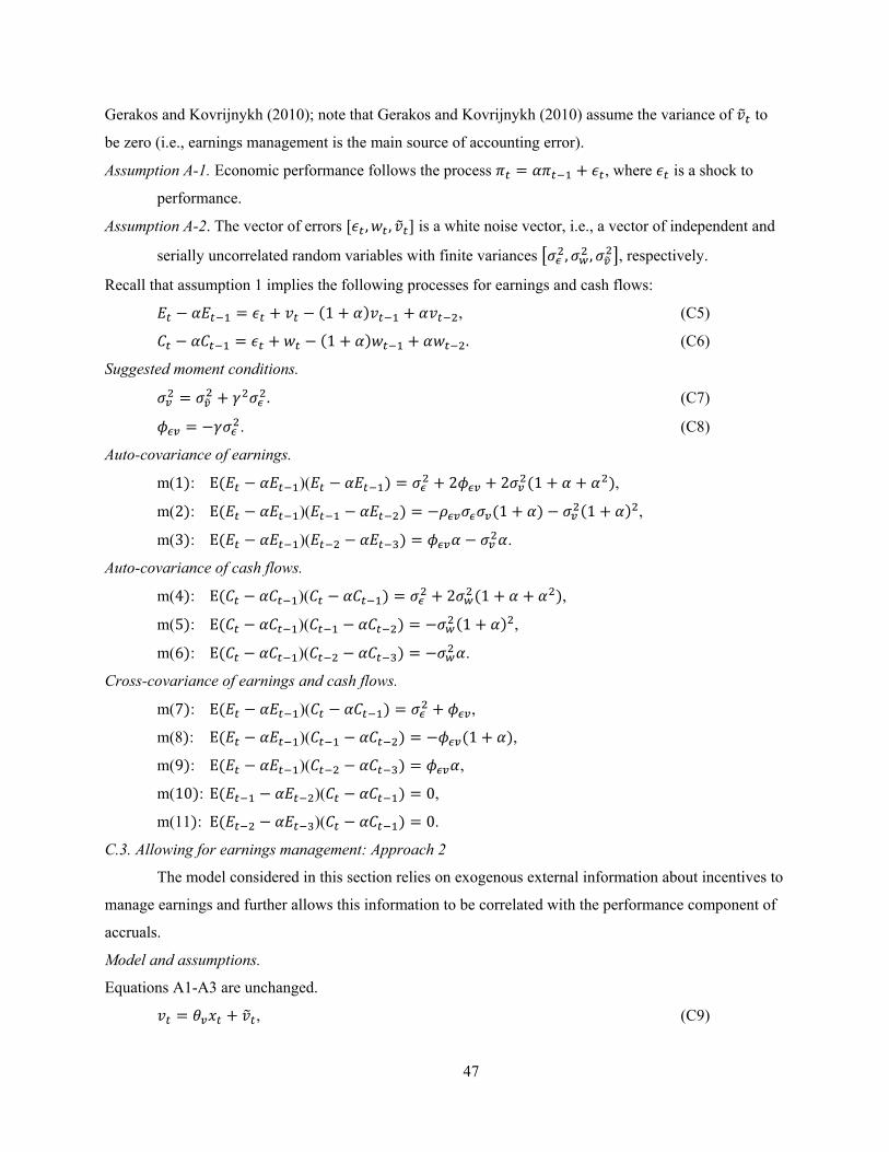
47
Gerakos and Kovrijnykh (2010); note that Gerakos and Kovrijnykh (2010) assume the variance of to
be zero (i.e., earnings management is the main source of accounting error).
Assumption A-1. Economic performance follows the process , where is a shock to
performance.
Assumption A-2. The vector of errors , , is a white noise vector, i.e., a vector of independent and
serially uncorrelated random variables with finite variances , , , respectively.
Recall that assumption 1 implies the following processes for earnings and cash flows:
1 , (C5)
1 . (C6)
Suggested moment conditions.
. (C7)
. (C8)
Auto-covariance of earnings.
m(1 : E )( 2 2 1 ,
m(2 : E )( 1 1 ,
m(3 : E )( .
Auto-covariance of cash flows.
m(4 : E )( 2 1 ,
m(5 : E )( 1 ,
m(6 : E )( .
Cross-covariance of earnings and cash flows.
m(7 : E )( ,
m(8 : E )( 1 ,
m(9 : E )( ,
m(10 : E )( 0,
m(11 : E )( 0.
C.3. Allowing for earnings management: Approach 2
The model considered in this section relies on exogenous external information about incentives to
manage earnings and further allows this information to be correlated with the performance component of
accruals.
Model and assumptions.
Equations A1-A3 are unchanged.
, (C9)

48
. (C10)
Assumption A-1. Economic performance follows the process , where is a shock to
performance.
Assumption A-2. The vector of errors , , is a white noise vector, i.e., a vector of independent and
serially uncorrelated random variables with finite variances , , , respectively.
Assumption A-3. Component (incentive to overstate performance) is serially uncorrelated and
independent of , , .
For convenience, is standardized to have zero mean and unity variance.
Suggested moment conditions.
, (C11)
, (C12)
. (C13)
Auto-covariance of earnings.
m(1): E )( 2 1 ,
m(2): E )( 1 ,
m(3): E )( .
Auto-covariance of cash flows.
m(4): E )( 2 1 ,
m(5): E )( 1 ,
m(6): E )( .
Cross-covariance of earnings and cash flows.
m(7): E )( 2 1 ,
m(8): E )( 1 ,
m(9): E )( ,
m(10): E )( 1 ,
m(11): E )( .
Covariance with the incentives for earnings management.
m(12): E ,
m(13): E .

49
Table 1: Summary statistics Panel A provides summary statistics for the variables used to estimate accounting quality parameters. E is earnings, C is cash flow, A is accruals, MV is the market value of equity, NA is non-current assets, M/B is the market value of equity plus total liabilities divided by total assets. Changes are denoted by Δ. The data is from Compustat and covers the 1987-2015 period. I use a cash flow statement approach to measure accruals. I exclude micro companies, foreign firms, ADRs, and firms in bankruptcy. Earnings, cash flow from operations, and accruals are scaled by beginning of period total assets. Changes are computed after the scaling is performed. All variables are demeaned in subsequent analysis. After the variables have been scaled, I exclude 1% of observations with extreme values both in the upper and lower tails of the distribution. I also require 15 observations with non-missing values per firm. Panel B provides summary statistics for the analysis of the determinants of accounting quality. The variables are based on Compustat and are averaged at firm level over the same time period that is used to estimate accounting quality parameters. I leave out the top and bottom 1% of extreme observations when I compute the averages. Panel A. Summary statistics for the estimation sample
Mean Std.Dev. 25% Median 75% E 0.0990 0.0896 0.0520 0.0951 0.1469 C 0.0887 0.0924 0.0405 0.0854 0.1386 A 0.0103 0.0550 -0.0132 0.0049 0.0301 ΔE -0.0015 0.0646 -0.0230 -0.0002 0.0206 ΔC -0.0006 0.0805 -0.0343 -0.0007 0.0323 ΔA -0.0008 0.0726 -0.0284 0.0000 0.0285 Δlog(MV) 0.0648 0.4918 -0.1666 0.0796 0.3129 Δlog(NA) 0.0737 0.2742 -0.0362 0.0397 0.1486 ΔM/B 0.0012 0.5781 -0.1569 0.0089 0.1696 N 47348 Panel B: Summary statistics for the firm-level determinants analysis Mean Std.Dev. 25% Median 75% Size 6.3548 2.0350 4.8516 6.3525 7.7192 Employees 0.6020 2.0383 -0.7990 0.6645 1.9946 Uncertainty 0.3216 0.1073 0.2361 0.3135 0.3960 B/M 0.6738 0.3804 0.4118 0.6115 0.8603 Leverage 0.2418 0.1741 0.1034 0.2170 0.3465 ROA 0.0285 0.0509 0.0072 0.0305 0.0563 Liquidity 0.1259 0.1202 0.0380 0.0829 0.1756 Days Inventory 0.5003 0.2888 0.2503 0.5003 0.7503 Days Receivables 0.5002 0.2887 0.2502 0.5002 0.7502 Asset life 14.3591 7.4249 9.3015 12.8744 17.6506 N 2238

50
Table 2: Performance vs. accounting error in accruals: Industry-level estimation The table presents the industry-level parameter estimates that characterize accounting quality. I use the annual time series of accruals, cash flow, and earnings from Compustat. The sample covers the period from 1987-2015. I use the cash flow statement approach to measure accruals. I exclude micro companies, foreign firms, ADRs, and firms in bankruptcy. Earnings, cash flow from operations, and accruals are scaled by beginning of period total assets. Changes are computed after the scaling is performed. I exclude 1% of observations with extreme values both in the upper and lower tails of the distribution. I also require 15 observations with non-missing values per firm. All variables are subsequently demeaned. I use the Fama and French (1997) 48 industry groups and require a minimum of 10 firms per industry. The estimates are based on the moment conditions in Section 3. Panel A contains the estimates based on the “levels” specification; Panel B is based on the specification using “changes”; Panel C is based on the generalized model specification (Approach 4, Section 3.4). Panel D presents from the Jones (1991) and Dechow and Dichev (2002) models estimated on the same data. The Dechow-Dichev model regresses accruals scaled by total assets on past, current, and future cash flows scaled by total assets. The Jones (1991) model regresses accruals on the change in revenue and the gross value of property, plant, and equipment all scaled by total assets. Panel A. "Levels" specification.
Variable Mean 25% Median 25% H0: Mean=0
t-value
N
0.0555 0.0483 0.0537 0.0555 39
0.0256 0.0194 0.0254 0.0256 39
0.0176 0.0128 0.0166 0.0176 39
0.0080 0.0041 0.0072 0.0080 9.50*** 39
/ 0.6788 0.6027 0.6739 0.7643
Panel B. "Changes" specification.
Variable Mean 25% Median 25% H0: Mean=0
t-value
N
0.0490 0.0402 0.0474 0.0551 39
0.0235 0.0180 0.0226 0.0279 39
0.0134 0.0094 0.0136 0.0166 39
0.0101 0.0072 0.0083 0.0128 11.49*** 39
/ 0.7458 0.6798 0.7605 0.8328
Panel C. Generalized specification.
Variable Mean 25% Median 25% H0: Mean=0
t-value
N
0.0559 0.0477 0.0551 0.0645 39
0.0259 0.0198 0.0263 0.0306 39
0.0155 0.0112 0.0145 0.0203 39
0.0103 0.0066 0.0089 0.0117 11.83*** 39
/ 0.7295 0.6739 0.7230 0.7827
Panel D. R-squareds from the Jones and Dechow-Dichev models.
Variable Mean 25% Median 25% N
Jones 1991 0.0721 0.0271 0.0734 0.1045 39
Dechow-Dichev 0.3468 0.2339 0.3544 0.4162 39

51
Table 3: Performance vs. accounting error in accruals: Firm-level estimation The table presents the firm-level parameter estimates that characterize accounting quality. I use the annual time series of accruals, cash flow, and earnings from Compustat. The sample covers the period from 1987-2015. I use the cash flow statement approach to measure accruals. I exclude micro companies, foreign firms, ADRs, and firms in bankruptcy. Earnings, cash flow from operations, and accruals are scaled by beginning of period total assets. Changes are computed after the scaling is performed. I exclude 1% of observations with extreme values both in the upper and lower tails of the distribution. I also require 15 observations with non-missing values per firm. All variables are subsequently demeaned. The estimates are based on the moment conditions in Section 3. Panel A contains the estimates based on the “levels” specification; Panel B is based on the specification using “changes”; Panel C is based on the generalized model specification (Approach 4, Section 3.4). Panel D presents from the Jones (1991) and Dechow and Dichev (2002) models estimated on the same data. The Dechow-Dichev model regresses accruals scaled by total assets on past, current, and future cash flows scaled by total assets. The Jones (1991) model regresses accruals on the change in revenue and the gross value of property, plant, and equipment all scaled by total assets. Panel A. "Levels" specification.
Variable Mean 25% Median 25% H0: Mean=0
t-value N
0.0517 0.0280 0.0444 0.0688 2238
0.0222 0.0110 0.0197 0.0311 2238
0.0153 0.0050 0.0120 0.0225 2238
0.0070 -0.0015 0.0062 0.0163 18.80*** 2238
/ 0.6461 0.4497 0.7056 0.9022 2238
Panel B. "Changes" specification.
Variable Mean 25% Median 25% H0: Mean=0
t-value N
0.0440 0.0197 0.0359 0.0618 2238
0.0205 0.0096 0.0178 0.0283 2238
0.0111 0.0026 0.0085 0.0157 2238
0.0093 0.0009 0.0075 0.0172 28.32*** 2238
/ 0.7119 0.5505 0.7859 0.9464 2238
Panel C. Generalized specification.
Variable Mean 25% Median 25% H0: Mean=0
t-value N
0.0518 0.0277 0.0443 0.0684 1962
0.0202 0.0100 0.0176 0.0279 1962
0.0110 0.0035 0.0088 0.0159 1962
0.0092 0.0009 0.0072 0.0166 29.42*** 1962
/ 0.7068 0.5413 0.7750 0.9393 1962
Panel D. from the Jones and Dechow-Dichev models.
Variable Mean 25% Median 25% N
Jones 1991 0.2398 0.0793 0.1892 0.3466 2238
Dechow-Dichev 0.4884 0.3056 0.4871 0.6672 2166
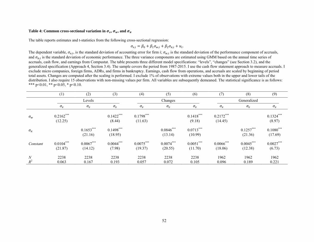
52
Table 4: Common cross-sectional variation in , , and
The table reports estimates and t-statistics from the following cross-sectional regression:
, , , .
The dependent variable, , , is the standard deviation of accounting error for firm ; , is the standard deviation of the performance component of accruals, and , is the standard deviation of economic performance. The three variance components are estimated using GMM based on the annual time series of accruals, cash flow, and earnings from Compustat. The table presents three different model specifications: “levels”, “changes” (see Section 3.2), and the generalized specification (Approach 4, Section 3.4). The sample covers the period from 1987-2015. I use the cash flow statement approach to measure accruals. I exclude micro companies, foreign firms, ADRs, and firms in bankruptcy. Earnings, cash flow from operations, and accruals are scaled by beginning of period total assets. Changes are computed after the scaling is performed. I exclude 1% of observations with extreme values both in the upper and lower tails of the distribution. I also require 15 observations with non-missing values per firm. All variables are subsequently demeaned. The statistical significance is as follows: *** p<0.01, ** p<0.05, * p<0.10. (1) (2) (3) (4) (5) (6) (7) (8) (9)
Levels Changes Generalized
0.2162*** 0.1422*** 0.1798*** 0.1418*** 0.2172*** 0.1324***
(12.25) (8.44) (11.63) (9.18) (14.45) (8.97)
0.1653*** 0.1498*** 0.0846*** 0.0713*** 0.1257*** 0.1080*** (21.16) (18.95) (13.14) (10.99) (21.36) (17.69) Constant 0.0104*** 0.0067*** 0.0044*** 0.0075*** 0.0074*** 0.0051*** 0.0066*** 0.0045*** 0.0027*** (21.87) (14.12) (7.98) (19.37) (20.55) (11.70) (18.06) (12.38) (6.73) N 2238 2238 2238 2238 2238 2238 1962 1962 1962 R2 0.063 0.167 0.193 0.057 0.072 0.105 0.096 0.189 0.221

53
Table 5: Determinants of the three variance components The table reports estimates and t-statistics from the following cross-sectional regression:
,
where Component is one of the three variance components: , – the standard deviation of accounting error for firm , , – the standard deviation of the performance component of accruals, and , – the standard deviation of economic performance. The variance components are estimated using GMM based on the annual time series of accruals, cash flow, and earnings from Compustat. The table presents three different model specifications: “levels”, “changes” (see Section 3.2), and the generalized specification (Approach 4, Section 3.4). Determinants are firm characteristics averaged over the period over which the variance components are estimated (I leave out 1% of extreme observations at the tails of the pooled distribution before averaging). Size is the average log of total assets, Employees is number of employees, Uncertainty is the difference between highest and lowest stock price over the fiscal year divided by their midpoint, B/M is the book value of equity divided by the market value of equity, Leverage is the ratio of long-term debt to total assets, Profitability is income before extraordinary items divided by total assets, Cash is the ratio of cash and cash equivalents to total assets, Days receivables is the cross-sectional (fractional) rank of days in receivables, i.e., the ratio of the average accounts receivable balance to sales per day, Days inventory is the cross-sectional (fractional) rank of days in inventory, i.e., the ratio of the average inventory balance to the cost of goods sold per day, Asset life is the ratio of gross value of property, plant, and equipment to depreciation expense. The sample covers the period from 1987-2015. I use the cash flow statement approach to measure accruals. I exclude micro companies, foreign firms, ADRs, and firms in bankruptcy. Earnings, cash flow from operations, and accruals are scaled by beginning of period total assets. Changes are computed after the scaling is performed. I exclude 1% of observations with extreme values both in the upper and lower tails of the distribution. I also require 15 observations with non-missing values per firm. All variables are subsequently demeaned. The statistical significance is as follows: *** p<0.01, ** p<0.05, * p<0.10.
(1) (2) (3) (4) (5) (6) (7) (8) (9)
Levels Changes Generalized
Size -0.0013*** -0.0018*** 0.0008 -0.0009*** -0.0017*** 0.0024*** -0.0009*** -0.0020*** -0.0004
(-4.90) (-5.17) (1.25) (-3.78) (-5.46) (3.58) (-4.01) (-6.39) (-0.66) Employees 0.0003 -0.0002 -0.0038*** 0.0002 -0.0002 -0.0053*** 0.0002 0.0001 -0.0027*** (1.08) (-0.51) (-6.00) (0.76) (-0.66) (-7.66) (0.66) (0.36) (-4.03) Uncertainty 0.0452*** 0.0235*** 0.1145*** 0.0304*** 0.0278*** 0.1142*** 0.0248*** 0.0238*** 0.1257*** (12.33) (5.16) (13.98) (9.52) (6.75) (12.72) (8.08) (5.63) (13.99) B/M -0.0023*** 0.0048*** -0.0202*** -0.0022*** 0.0039*** -0.0170*** -0.0017** 0.0038*** -0.0204*** (-2.89) (4.97) (-11.51) (-3.22) (4.39) (-8.83) (-2.53) (4.01) (-10.28) Leverage -0.0080*** -0.0097*** -0.0230*** -0.0077*** -0.0115*** -0.0259*** -0.0059*** -0.0108*** -0.0241*** (-3.70) (-3.59) (-4.72) (-4.08) (-4.71) (-4.87) (-3.25) (-4.32) (-4.54)

54
Profitability -0.0147** 0.0205** -0.0891*** -0.0163*** 0.0180** -0.0961*** -0.0177*** 0.0209*** -0.0928*** (-2.18) (2.46) (-5.94) (-2.78) (2.39) (-5.84) (-3.07) (2.63) (-5.52) Cash -0.0053* -0.0058* 0.0587*** -0.0033 -0.0064** 0.0488*** -0.0006 -0.0066** 0.0508*** (-1.87) (-1.66) (9.32) (-1.33) (-2.03) (7.07) (-0.25) (-2.01) (7.33) Days Inventory 0.0080*** 0.0077*** -0.0037* 0.0043*** 0.0072*** -0.0035 0.0049*** 0.0080*** -0.0012 (8.73) (6.82) (-1.81) (5.36) (7.00) (-1.55) (6.54) (7.74) (-0.55) Days Receivables 0.0048*** -0.0013 -0.0076*** 0.0047*** -0.0019 -0.0069*** 0.0025*** -0.0002 -0.0047* (4.55) (-0.96) (-3.24) (5.20) (-1.65) (-2.70) (2.90) (-0.18) (-1.90) Asset life -0.0001** -0.0002*** -0.0003*** -0.0001 -0.0002*** -0.0001 -0.0001 -0.0002*** -0.0002** (-2.05) (-4.44) (-2.66) (-1.44) (-3.47) (-1.09) (-1.51) (-3.54) (-2.28) Constant 0.0092*** 0.0265*** 0.0371*** 0.0081*** 0.0237*** 0.0182*** 0.0097*** 0.0252*** 0.0410***
(3.58) (8.26) (6.41) (3.60) (8.15) (2.88) (4.52) (8.54) (6.55)
N 1870 1870 1870 1870 1870 1870 1658 1658 1658 R2 0.359 0.253 0.467 0.270 0.286 0.399 0.276 0.305 0.471

55
Table 6: Differential audit pricing implications of accounting error vs. the performance component The table presents the estimates and t-statistics from the following regression:
log ∑ .
Audit Fee is total audit fees, , is the standard deviation of accounting error for firm , , is the standard deviation of the performance component of accruals, and , is the standard deviation of economic performance. Control variables include the following: Size – log of is total assets, Employees – the number of employees, Leverage – the sum of long-term and short-term debt divided by total assets, B/M – the ratio of book value of equity to market value of equity, R&D – the ratio of research and development expense to total assets, Cash – the ratio of cash to total assets, Loss – dummy for negative income before extraordinary items, Tenure – the number of years that the firm has been a client of the current auditor, #Segments – the number of business segments, Acquisition – dummy variable for acquisition in excess of 5% of total assets, DiscOp – dummy for discontinued operations in excess of 5% of total assets, Restruct – dummy for restructuring charges in excess of 5% of total assets, EquityIss – dummy for equity issuance in excess of 5% of total assets, DebtIss – dummy for debt issuance in excess of 5% of total assets, December – dummy for the December fiscal year end, Big4 – the indicator for the firm’s auditor being a member of the Big 4 (Big 5 before the exit of Arthur Andersen). The data of audit fees comes from Audit Analytics and begins in 2000. The standard errors are clustered by firm. The robust t-statistics clustered by company are in parenthesis. The statistical significance is as follows: *** p<0.01, ** p<0.05, * p<0.10.
(1) (2) (3) (4) (5) (6)
Levels Changes Generalized
Audit Fees Audit Fees Audit Fees Audit Fees Audit Fees Audit Fees
12.5295*** 6.5598*** 13.4772*** 6.7582*** 15.0700*** 8.5434*** (11.10) (6.70) (10.39) (6.07) (9.00) (5.91)
6.5448*** 2.6661*** 8.7192*** 3.8529*** 9.4439*** 4.2984*** (6.43) (3.16) (8.11) (4.41) (8.12) (4.10)
2.1385*** 0.4776 2.2577*** 1.0753*** 2.1997*** 0.3381 (4.59) (1.13) (5.12) (3.05) (4.22) (0.69)
Controls - Yes - Yes - Yes
N 25010 24110 25010 24110 22469 21757 R2 0.704 0.746 0.703 0.746 0.710 0.749

56
Table 7: Differential audit pricing implications of accounting error vs. performance component: Audit fees scaled by total assets
The table presents the estimates and t-statistics from the following regression:
∑ ,
Audit Fee is total audit fees, , is the standard deviation of accounting error for firm , , is the standard deviation of the performance component of accruals, and , is the standard deviation of economic performance. Control variables include the following: Size – log of is total assets, Employees – the number of employees, Leverage – the sum of long-term and short-term debt divided by total assets, B/M – the ratio of book value of equity to market value of equity, R&D – the ratio of research and development expense to total assets, Cash – the ratio of cash to total assets, Loss – dummy for negative income before extraordinary items, Tenure – the number of years that the firm has been a client of the current auditor, #Segments – the number of business segments, Acquisition – dummy variable for acquisition in excess of 5% of total assets, DiscOp – dummy for discontinued operations in excess of 5% of total assets, Restruct – dummy for restructuring charges in excess of 5% of total assets, EquityIss – dummy for equity issuance in excess of 5% of total assets, DebtIss – dummy for debt issuance in excess of 5% of total assets, December – dummy for the December fiscal year end, Big4 – the indicator for the firm’s auditor being a member of the Big 4 (Big 5 before the exit of Arthur Andersen). The data of audit fees comes from Audit Analytics and begins in 2000. The standard errors are clustered by firm. The robust t-statistics clustered by company are in parenthesis; *** p<0.01, ** p<0.05, * p<0.10.
(1) (2) (3) (4) (5) (6)
Levels Changes Generalized
Fees/Assets Fees/Assets Fees/Assets Fees/Assets Fees/Assets Fees/Assets
0.0523*** 0.0185*** 0.0626*** 0.0223*** 0.0550*** 0.0211*** (10.56) (5.18) (10.61) (5.17) (8.03) (4.21)
0.0286*** 0.0011 0.0375*** 0.0034 0.0342*** 0.0028 (8.54) (0.44) (10.12) (1.18) (8.96) (0.94)
0.0198*** 0.0049*** 0.0199*** 0.0059*** 0.0201*** 0.0054*** (9.66) (3.30) (10.99) (4.61) (9.40) (3.53) Controls - Yes - Yes - Yes N 25177 24258 25177 24258 22623 21893 R2 0.262 0.492 0.262 0.493 0.266 0.497