Identify Parameters Important to Predictions using PPR

& Identify Existing Observation

Locations Important to Predictions using OPR

PPR Statistics for Exercise 8.1c

• Files are provided for 2 analyses :

1. MODE=PPR, PARGROUPS=NO – If we could obtain data on any one parameter, which should it be?

2. MODE=PPR, PARGROUPS=YES, 2 parameters per group – If we could obtain data on any pair of parameters, which should they be?

10 yrs

50 yrs

100 yrs

175 yrs

50 yr

Riv

er

Well

100 yr

10 yr

True particleposition at:

Predicted pathConfidence intervalTrue path

PPR – Exercise 8.1c• Prediction is the advective transport at

100 years travel time.

• PercentReduc=10

• What if we could collect data to reduce by 10 percent the parameter standard deviation?

- PPR = percent decrease in the standard deviation of a prediction produced by a 10-percent decrease in the standard deviation of the parameter.

• Results for the advective-transport predictions at 100 years are shown in next slides:

• First – individual parameters

• Second – pairs of parameters

x

y

Figure 8.15b, p. 210

Exercise 8.1c: PPR Individual Parameters

• Which parameters rank as most important to the predictions by the ppr statistic?

• With CSS and PSS, HK_2 and POR1&2 were ranked first.

• Why the difference for POR1&2???

0

2

4

6

8

10

HK_1 K_RB VK_CB HK_2 RCH_1 RCH_2 POR_1&2

Parameter Name

Ave

rage

ppr

sta

tist

ic

(a)

Average ppr statistic for all predictions

Figure 8.9a, p. 201

1 2 3

Changes in meters are small for A100z compared to A100x & A100y. But the vertical dimension is much smaller. PPR correctly represents the different dimensions.

PPR Change,in meters

0

2

4

6

8

10

K_RB andPOR_1&2

All otherparameters

ppr

stat

isti

cA100xA100yA100z

(b)

1

10

100

1000

10000

K_RB andPOR_1&2

All otherparameters

(c)

Ave

rage

dec

reas

e in

pre

dict

ion

stan

dard

dev

iati

on (

met

ers)

Exercise 8.1c: PPR Individual Parameters

Figure 8.9b, p. 201 Figure 8.9c, p. 201

Exercise 8.1c: PPR Grouped Parameters

• Which parameter pairs would be most beneficial to simultaneously investigate?

0

5

10

15

20

All pairs thatinclude K_RB or

POR_1&2

All other pairs

(d)

Ave

rage

ppr

stat

isti

c

Figure 8.9d, p. 201

Any pair of:HK_1 RCH_1VK_CB RCH_2HK_2

Kind of surprising!

How is PPR calculated???

• OPR and PPR statistics are based on the calculation of prediction standard deviation, a measure of prediction uncertainty

Predictions – Advective TravelPrediction• UCODE_2005 can compute

the sensitivity of the predicted travel path in three directions:• X - East-West• Y - North-South• Z - Up-Down

• Using calculations described later, the variance and / or standard deviation of predictions can be determined

Advective path

Predictions – Uncertainty

Standard Deviation

• Measure of spread of values for a variable

• Involves assumptions

• Used in OPR & PPR statistics as a means for comparing relative predictive uncertainty

• The black curve presents the standard deviation in the context of a normal distribution, which may or not be the appropriate distribution for this uncertainty.

Normal distribution

Advective path

Predictions – UncertaintyStandard Deviation

• With additional information on parameters or with additional observations – predictive standard deviation is reduced

• Red bars illustrates ‘new’ predictive standard deviation

• The change in standard deviation makes the probability distribution more narrow.

• Use the difference between the red and the black bars to measure the worth of the additional data

Normal distribution

Advective path

Normal distribution

Predictions – UncertaintyStandard Deviation

• With the omission of information about one or more observations – predictive standard deviation is increased

• Red bars illustrate ‘new’ predictive standard deviation

• The change in standard deviation makes the probability distribution wider.

• Use the difference between the red and the black bars to measure the worth of the omitted data

Normal distribution

Advective path

Standard deviation of a prediction

standard deviation of the th simulated prediction, z’calculated error variance from regressionvector of prediction sensitivities to parametersmatrix of observation sensitivities to parametersmatrix of weights on observations and priortranspose the matrixparameter variance-covariance matrix

sz’

s2

z’b X

V(b)

sz’ = [s2 ( (XTX)-1 )]1/2

V(b) = s2(XTX)-1

z’b

z’T

b

Standard deviation of a prediction

• All terms in this equation are already available• weight matrix includes weights on observations and on

prior information about parameters• sensitivity matrix X contains the sensitivities for simulated

equivalents to the observations, and entries for prior information on parameters

• First order second moment (FOSM) method• First order – linearise using first order Taylor’s series• Second moment – variances and standard deviations

• For OPR and PPR statistics, manipulate and X

sz’ = [s2 ( (XTX)-1 )]1/2z’b

z’T

b

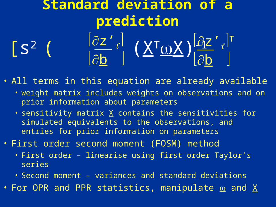
Standard deviation of a prediction

• All terms in this equation are already available• weight matrix includes weights on observations and on

prior information about parameters• sensitivity matrix X contains the sensitivities for simulated

equivalents to the observations, and entries for prior information on parameters

• First order second moment (FOSM) method• First order – linearise using first order Taylor’s series• Second moment – variances and standard deviations

• For OPR and PPR statistics, manipulate and X

sz’ = [s2 ( (XTX)-1 )]1/2z’b

z’T

b

X and

X

NPNPRNPRNPR

NP

NP

NPNDNDND

NP

NP

aaa

aaa

a

x

a

x

a

x

xxx

xxx

,2,1,

,22,21,2

,1

,

2,1

2,

1,1

,

,22,21,2

,12,11,1

..

..

..

1

U

W

0

0

Observation part

Sensitivities

Weighting

Prior information part

X and

X

NPNPRNPRNPR

NP

NP

NPNDNDND

NP

NP

aaa

aaa

a

x

a

x

a

x

xxx

xxx

,2,1,

,22,21,2

,1

,

2,1

2,

1,1

,

,22,21,2

,12,11,1

..

..

..

1

U

W

0

0

Observation part

Sensitivities

Weighting

Prior information part

For PPR add Prior Information terms

For OPR add or remove observation

terms

• Calculate the prediction standard deviation using calibrated model and existing observations

• Calculate hypothetical prediction standard deviation assuming changes in information about parameters or changes to the available observations

• The Parameter-Prediction (PPR) Statistic:

• Evaluate worth of potential new knowledge about parameters, posed in the form of prior information - add to calculations

• The Observation-Prediction (OPR) Statistic:

• Evaluate existing observation locations - omit from calculations

• Evaluate potential new observation locations – add to calculations

OPR and PPR Statistics - Approach

OPR-PPR Program

• Encapsulates OPR and PPR statistics:

• Compatible with the JUPITER API and UCODE_2005

• Distributed with MF2K2DX that will convert MODFLOW-2000 and MODFLOW-2005 output files into the Data-Exchange Files needed by OPR-PPR ***ask Matt

• Tonkin, Tiedeman, Ely, Hill (2007) Documentation for OPR-PPR, USGS Techniques & Methods 6-E2

• Exercise uses the OPR and PPR methods together with the synthetic model

PPR Statistic Calculation

• The PPR statistic is defined as the percent change in prediction standard deviation caused by increased knowledge about the parameter

• Therefore it measures the relative importance to a prediction of potential new information on a parameter

sz’ = [s2( (XT X)-1 )]1/2(j)

z’b

z’T

b (j)

ppr = [1- (sz / sz)] x 100(j)(j)

PPR Statistic - Theory

Focusing on ppr:

• Weights on the potential new information are ideally proportional to the uncertainty in that information

• But, it is not known how certain this information will be

• This is overcome pragmatically by calculating the weight that that reduces the parameter standard deviation by a user specified percentage.

Y,PRIppr

Weights on existing observations and prior

Weights on potential new information on parameters

(j)

PPR Statistic - Theory

Calculating weights on potential new information:

• User specifies the desired percent reduction (‘PercentReduc’) in the parameter standard deviation

• Within OPR-PPR:

• Add a nominal initial weight into the weight matrix ppr for the

corresponding parameter

• Iteratively solve the equations above until the standard deviation in that parameter is reduced by the user-specified amount

• Calculate sz

OPR Statistic Calculation

• The OPR statistic is defined as the percent change in prediction standard deviation caused by:

the addition of one or more observations – OPR-ADDthe omission of one or more observations – OPR-OMIT

[1- (sz / sz)] x 100(i)

sz’ = [s2( (XT X )-1 )]1/2(i)

z’b

z’T

b (i) (i)(i)

OPR Statistic - Theory

• Weights on existing observations already determined

• Weights on potential observations must be determined using same guiding principles

Y,PRI

Weights on existing observations and prior

OPR Statistic - Calculation

OBSOMIT STEPS:

• Set weight(s) for relevant observation(s) to zero

• Sensitivity matrix X does not need to be modified

• Calculate sz

OBSADD STEPS:

• Calculate sensitivities for potential observations and append these to X

• Construct weights for potential observations and append these to Y,PRI

• Calculate sz

Exercise 8.1d: OPR Statistic

Use MODE=OPROMIT, OBSGROUPS=NO to analyze

the individual omission of the existing head and flow

observations and identify which of these

observations are most important to the predictions.

Exercise 8.1d – OPR Statistic Results

• Which observations rank as most important to the predictions?

• Why? Use:dss – Table 7.5 (p. 148)pss – Figure 8.8 (p. 198)pcc – Information in Table 8.6 (p. 204)

0

10

20

30

40

50

60

70

hd01

.ss

hd02

.ss

hd03

.ss

hd04

.ss

hd05

.ss

hd06

.ss

hd07

.ss

hd08

.ss

hd09

.ss

hd10

.ss

flow

01.s

s

Observation name

A100x

A100y

A100z

opr

sta

tist

ic (

perc

ent

incr

ease

in

pred

icti

on s

tand

ard

devi

atio

n)

Figure 8.10a, p. 203

OPR

Exercise 8.1d – OPR Statistic Results

• Does analysis of the absolute increases in prediction standard deviation produce the same conclusions as did analysis of the opr statistics on the previous slide?

Figure 8.10b, p. 203

Change, in meters

1

10

100

1000

10000

100000

hd01

.ss

hd02

.ss

hd03

.ss

hd04

.ss

hd05

.ss

hd06

.ss

hd07

.ss

hd08

.ss

hd09

.ss

hd10

.ss

flow

01.s

s

Observation name

A100x

A100y

A100z

Incr

ease

in p

redi

ctio

n st

anda

rdde

viat

ion

(met

ers)