identification of young stellar objects ... - pavan vynatheya
TRANSCRIPT
Page 1 of 30
Identification of Young Stellar
Objects in NGC 7538 using Spitzer
archive data
PAVAN VYNATHEYA
BS-MS STUDENT
IISER KOLKATA
Supervisor:
DR. SAURABH SHARMA
SCIENTIST ‘D’
ARIES NAINITAL

Page 2 of 30
1 INTRODUCTION
1.1 STAR FORMATION
Star formation is the process in which dense regions of molecular
clouds condense into protostars. Molecular clouds are relatively dense
regions of interstellar matter made up mostly of hydrogen, present in
its molecular form.
Molecular clouds can vary vastly in size. The smallest ones are called
Bok Globules, whose masses are less than a few hundred Solar masses.
The largest ones, Giant Molecular Clouds (GMCs) have masses of about
105 Solar Masses and are spread across hundreds of light years. Their
temperatures range around 10-20 K.
The fundamental requirement for star formation is that the ‘inward’
gravitational force (potential energy) must exceed the ‘outward’ gas
pressure (kinetic energy). The virial theorem states that for hydrostatic
equilibrium (of a molecular cloud), the potential energy must be twice
that of the kinetic energy. If the mass of a cloud exceeds the ‘Jeans
mass’, it will undergo gravitational collapse. The Jeans instability
criterion depends on the temperature and density of a cloud.
Molecular clouds break into clumps, which in turn collapse to form
individual protostars. These clumps are denser parts of the cloud. This
results in the formation of a cluster of stars, which may stay together or
drift apart.
Star formation can also be ‘triggered’. This can occur due to
shockwaves from a nearby supernova explosion or galactic collision.
Triggered formation can also occur in the vicinities of HII regions
(consisting of ionized hydrogen rather than molecular hydrogen).
After the clump or the cloud collapses, a protostar is born, which
further evolves into a star.
Page 3 of 30
1.2 YOUNG STELLAR OBJECTS (YSOS)
YSOs denote the early phase of stellar evolution. There are two groups
of YSOs – protostars and pre-main sequence (PMS) stars.
A Protostar is the first stage of stellar evolution. When a molecular
clump starts collapsing, it is called a protostar. When this happens, it
starts spinning to form a spherical clump. The outer material forms a
envelope, which eventually becomes a circumstellar disc (site for
planet formation). Initially, the clump is transparent to radiation. As
the density increases, it becomes opaque. Escaping IR radiation is
trapped, resulting in increase in pressure and temperature of the
protostar. The protostar gains mass as more material is accreted from
the envelope.
A protostar becomes a PMS star when it blows away its outer envelope
and becomes optically visible. A PMS star generates heat by
gravitational contraction, and not by hydrogen burning. The star
continues to collapse until its pressure and temperature are high
enough for hydrogen fusion. When this happens, it is said to be a main
sequence star. A PMS star, thus, has a higher radius than a main
sequence star of similar mass. It also has a circumstellar disc, which
eventually gets dissipated by accretion and planet formation. This disc
is responsible for emission in far IR.
A PMS star can either be a T Tauri star (less than 2 Solar masses) or a
Herbig Ae/Be star (2-8 Solar masses). Stars with masses greater than 8
Solar masses contract too quickly to have a pre-main sequence stage;
they are already main-sequence stars.
Based on the stage of evolution, YSOs are classified into different
classes. The classification is done based on the Spectral Energy
Distributions (SEDs) of the YSOs.

Page 4 of 30
1.3 CLASSES OF YSOS
The SED is a plot of brightness (or flux density) vs. wavelength (or
frequency) of light. Based on their SEDs, YSOs are classified into four
classes (see Fig 1.) –
• Class 0 – They are protostars that are extremely faint in optical
and near IR regions, but are luminous in submillimeter
wavelengths.
• Class I – They are embedded sources with circumstellar discs and
envelopes, which peak in the mid-IR to far-IR regions and are
optically invisible.
• Class II – They have significant circumstellar discs, strong
emission lines and IR and optical luminosities.
• Class III – They don’t have circumstellar discs and weak emission
lines.
Fig 1: Typical SEDs of the various classes of YSOs (Flux density vs. frequency).
Page 5 of 30
1.4 NGC 7538
NGC 7538 is an active Star Forming Region (SFR) in the constellation Cepheus, about 2.7 kpc from the Earth. Right Ascension and Declination of NGC 7538 are approximately 348.4° and 61.4°.
Since NGC 7538 is an SFR, it emits significantly in the infrared region of the EM spectrum. Thus, data from the Spitzer Space Telescope (SST), an infrared space telescope is used to gather this data.
1.5 SPITZER SPACE TELESCOPE (SST)
The SST is an infrared space telescope launched by NASA in 2003 as a
part of the NASA ‘Great Observatories’ program. The other missions
were the visible-light Hubble Space Telescope (HST), the Compton
Gamma-Ray Observatory (CGRO) and the Chandra X-Ray Obserbatory
(CXO).
The Spitzer carries three instruments on board –
• Infrared Array Camera (IRAC) – An infrared camera which
operates simultaneously on four wavelength ‘channels’ – 3.6 µm,
4.5 µm, 5.8 µm and 8.0 µm. Each module uses a 256×256 pixel
detector.
• Infrared Spectograph (IRS) – An infrared spectrometer with four
sub-modules which operate at the wavelengths 5.3–14 µm (low
resolution), 10–19.5 µm (high resolution), 14–40 µm (low
resolution), and 19–37 µm (high resolution). Each module uses a
128×128 pixel detector.
• Multiband Imaging Photometer for Spitzer (MIPS) – Three
detector arrays in the far IR – 128×128 pixels at 24 µm, 32×32
pixels at 70 µm, 20×20 pixels at 160 µm.
All Spitzer data is freely available online in the Spitzer Heritage
Archive (SHA). Only IRAC data has be used in this project.
Page 6 of 30
1.6 TWO MICRON ALL SKY SURVEY (2MASS)
The 2MASS was an infrared astronomical survey of the whole sky in
the infrared spectrum which took place between 1997 and 2001. Two
1.3-m telescopes were used for the survey, one in Arizona, USA
(Northern Hemisphere) and the other in Chile (Southern Hemisphere).
Observations were taken in three wavelength bands – J (1.235 µm), H
(1.662 µm) and K (2.159 µm). The three channel cameras used
256×256 arrays. 2MASS data is available at the Infrared Science
Archive (IRSA).
1.7 IMAGE REDUCTION AND ANALYSIS FACILITY (IRAF)
IRAF is a software collection written at the National Optical
Astronomical Observatory (NOAO) used primarily for data reduction
and photometry. One specific package of IRAF used in this project is
DAOPHOT.
DAOPHOT is a package for stellar photometry designed to deal with
crowded fields. More details about this package (commands and
parameters) are given in future sections.
1.8 MOSAICKER AND POINT SOURCE EXTRACTOR (MOPEX)
MOPEX is a software used for reducing and analyzing imaging data, and
for creating mosaic images. MOPEX comes in two modes – Graphical
User Interface (GUI) mode and Command Line mode.
In this project, MOPEX has been used in the Command Line mode. More
details of the commands and various processes involved are given in
future sections.
Page 7 of 30
1.9 PYTHON SED FITTER
The Spectral Energy Distribution (SED) fitter is a Python package used
for fitting given data (YSO data) to their SEDs. It has various models
which fit stars with data, in at least five wavelength bands, to the SED
with least deviation.
It also lists various parameters of stars, including calculated masses
and ages, in a separate output file. SED fitting is done after YSOs of
various classes are identified (in this case, Classes I and II only). The
Python code and other details are given in future sections.
2 MY PROJECT
2.1 OBJECTIVE
To create mosaic images of NGC 7538 in the four IRAC channels (3.6
µm, 4.5 µm, 5.8 µm, 8.0 µm), conduct photometry in each of the bands,
identify YSOs using specific techniques and fit their SEDs.
2.2 PROCEDURE (OVERVIEW)
The procedure followed in this project is as follows –
i. The data from the SHA is basically a collection of .fits image files
(in all four channels). They consist of basic calibrated data
(*bcd.fits), corresponding uncertainty files (*bunc.fits) and image
masking files (*bimsk.fits). These files need to be overlapped and
mosaicked using MOPEX (Mosaicker and Point-Source Extractor).
ii. Photometry is carried out using one of IRAF’s (Image Reduction
and Analysis Facility) packages called digiphot. Its subpackage
daophot has various commands, which make photometry a simple
matter of using the right ones.
Page 8 of 30
iii. The output is a list of all stars, along with their various
parameters (positions, magnitudes, errors) in all four channels.
The next step is to match the stars in all the channels using the
tmatch command in the stsdas package of IRAF. This finally gives
us a comprehensive list of stars detected in all four wavelength
bands.
iv. The most crucial process is the identification of YSOs from this
list. This can be done by filtering the stars using the process
described in the Appendix A of the paper by Gutermuth et al. 2009.
v. Finally, SED fitting for the filtered Class I and Class II is carried out
using the Python SED Fitter package, and the output plots are
identified. The process more or less follows what is done in the
paper by Sharma et al. 2016.
2.3 IMAGE MOSAICKING USING MOPEX
As mentioned before, data from the SHA is divided into various
directories containing *bcd.fits, *bunc.fits and *bimsk.fits image files.
Firstly, appropriate input list files for MOPEX are made. The various
steps followed are as follows –
i. A list file containing all of the above mentioned file path names
(absolute) is made. The LINUX find command is used for this task.
Moreover, the even-numbered (short exposure) and the odd-
numbered (long exposure) files are separated (more on this
later). The find command, unfortunately, lists only the relative
path names of the .fits files. This can be remedied using the LINUX
sed command, which replaces a certain string with another string.
ii. The above file list is sorted numerically using the LINUX sort
command. This is necessary because MOPEX reads only sorted
data. Now, there are six list files – two (short and long) for each of
the *bcd.fits, *bunc.fits and *bimsk.fits image files.
Page 9 of 30
iii. The LINUX grep command is used to read each of the six list files,
and further separate them based on their wavelength channel.
Now, there are 24 list files.
iv. One must make sure that each of the six files (for a particular
channel) has the same number of lines. In other words, they must
have same number of image files listed. If, by chance, it is not so,
then they must be made so. This is very necessary to run MOPEX.
(Note – This is not the only method in which the input list files can
be made. This is the method I have used.)
The next step is to feed these input files into MOPEX. This input is
given through .nl name list files. These files are present (by default)
in the cdf directory of MOPEX. The syntax is ready-made and the
only information to fill in are the addresses of the various input list
files and output .fits mosaic files. Three .nl files are used for each
channel. They are as follows (to be run in chronological order) –
i. overlap*.nl – The input to this is the list file containing long
exposure .fits images. The output is a .fits image and another list
file. The command overlap.pl –n overlap*.nl is used to overlap all
the long exposure files (of a particular channel) and create an
overlapped image.
ii. hdr_mask*.nl – The inputs to this are the list file containing short
exposure .fits images and the output list file of the previous
command. The output is a .fits image and another list file. The
command hdr_mask.pl –n hdr__mask*.nl is used to combine the
short exposure and long exposure files (of a particular channel)
and create an image which has both. This is necessary because
long exposures tend to saturate images, and thus must be dealt
with separately.
iii. mosaic*.nl – The input to this is the output list file of the previous
command. The output is a .fits image. The command mosaic.pl –n
Page 10 of 30
mosiac*.nl is used to create a mosaic image (of a particular
channel), which is the final output of MOPEX.
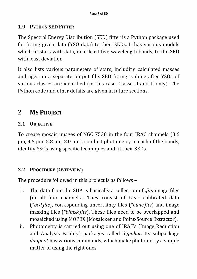
When all three tasks are performed, a mosaic.fits image (for each
channel) is created. Now, these images are ready for photometry,
which is done using IRAF DAOPHOT (see Fig 2.).
(a) (b)
(c) (d)
Fig 2: The mosaic images of NGC 7538 after using MOPEX displayed using
SAOImage DS9 (image displayer). (a) ch1 (b) ch2 (c) ch3 (d) ch4
Page 11 of 30
2.4 PHOTOMETRY USING IRAF DAOPHOT
As mentioned before, the main photometry subpackage of IRAF is
daophot, which can be found in the package digiphot. An essential part
after photometry is point spread function (PSF) correction, which can
also be done using daophot. The PSF describes the response of an
imaging system to a point source. In other words, point sources are not
seen as point sources, but are spread over multiple pixels.
Before carrying out all the daophot commands, one must make sure all
their parameters are adjusted according to one’s needs, which can be
edited using the command epar. They are –
• findpars – Star detection parameters (detection threshold
threshold, mark detections mkdetections)
• datapars – General star parameters (full-width half-maximum of
PSF fwhmpsf, standard deviation of sky background sigma,
minimum and maximum good data values datamin and datamax).
• centerpars – Centering parameters (centering algorithm
calgorithm, center data width cbox).
• fitskypars – Sky fitting parameters (sky fitting algorithm
salgorithm, sky annulus annulus and dannulus).
• photpars – Aperture parameters (aperture radius apertures, zero
magnitude zmag).
• daopars – PSF parameters (PSF radius psfrad, fitting radius
fitrad).
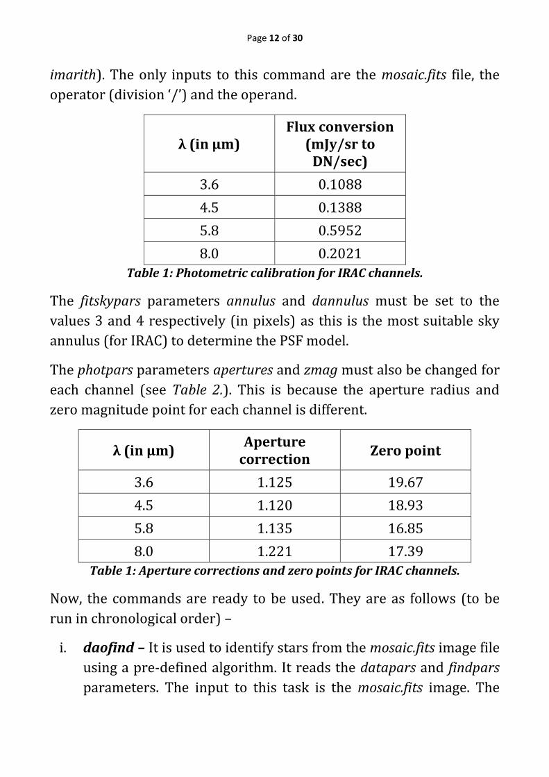
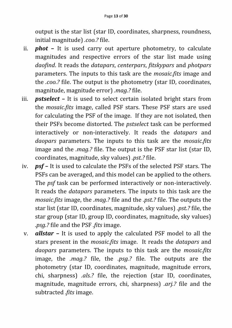
For the four IRAC channels, there are a few parameters which need to
be edited. First of all, the images in the four channels must be
calibrated so that their fluxes normalize. This is done by dividing the
respective mosaic.fits images by certain pre-determined factors (see
Table 1.). This can be done using a command imarith in the
subpackadge ccdred of the package imred (IRAF > imred > ccdred >
Page 12 of 30
imarith). The only inputs to this command are the mosaic.fits file, the
operator (division ‘/’) and the operand.
λ (in µm)
Flux conversion (mJy/sr to
DN/sec)
3.6 0.1088
4.5 0.1388
5.8 0.5952
8.0 0.2021
Table 1: Photometric calibration for IRAC channels.
The fitskypars parameters annulus and dannulus must be set to the
values 3 and 4 respectively (in pixels) as this is the most suitable sky
annulus (for IRAC) to determine the PSF model.
The photpars parameters apertures and zmag must also be changed for
each channel (see Table 2.). This is because the aperture radius and
zero magnitude point for each channel is different.
λ (in µm) Aperture
correction Zero point
3.6 1.125 19.67
4.5 1.120 18.93
5.8 1.135 16.85
8.0 1.221 17.39
Table 1: Aperture corrections and zero points for IRAC channels.
Now, the commands are ready to be used. They are as follows (to be
run in chronological order) –
i. daofind – It is used to identify stars from the mosaic.fits image file
using a pre-defined algorithm. It reads the datapars and findpars
parameters. The input to this task is the mosaic.fits image. The
Page 13 of 30
output is the star list (star ID, coordinates, sharpness, roundness,
initial magnitude) .coo.? file.
ii. phot – It is used carry out aperture photometry, to calculate
magnitudes and respective errors of the star list made using
daofind. It reads the datapars, centerpars, fitskypars and photpars
parameters. The inputs to this task are the mosaic.fits image and
the .coo.? file. The output is the photometry (star ID, coordinates,
magnitude, magnitude error) .mag.? file.
iii. pstselect – It is used to select certain isolated bright stars from
the mosaic.fits image, called PSF stars. These PSF stars are used
for calculating the PSF of the image. If they are not isolated, then
their PSFs become distorted. The pstselect task can be performed
interactively or non-interactively. It reads the datapars and
daopars parameters. The inputs to this task are the mosaic.fits
image and the .mag.? file. The output is the PSF star list (star ID,
coordinates, magnitude, sky values) .pst.? file.
iv. psf – It is used to calculate the PSFs of the selected PSF stars. The
PSFs can be averaged, and this model can be applied to the others.
The psf task can be performed interactively or non-interactively.
It reads the datapars parameters. The inputs to this task are the
mosaic.fits image, the .mag.? file and the .pst.? file. The outputs the
star list (star ID, coordinates, magnitude, sky values) .pst.? file, the
star group (star ID, group ID, coordinates, magnitude, sky values)
.psg.? file and the PSF .fits image.
v. allstar – It is used to apply the calculated PSF model to all the
stars present in the mosaic.fits image. It reads the datapars and
daopars parameters. The inputs to this task are the mosaic.fits
image, the .mag.? file, the .psg.? file. The outputs are the
photometry (star ID, coordinates, magnitude, magnitude errors,
chi, sharpness) .als.? file, the rejection (star ID, coordinates,
magnitude, magnitude errors, chi, sharpness) .arj.? file and the
subtracted .fits image.
Page 14 of 30
The four (for each channel) .als.? files are the final products of
photometry. The only thing left to do now is to identify the YSOs in the
star list.
2.5 FILTERING YSOS
The first thing to be done is to extract the column data from the .als file.
This is done using the txdump command of IRAF (IRAF > txdump). The
star ID, coordinates, magnitude, magnitude error, chi and sharpness
columns are extracted.
cl> txdump *.als.? ID, XCENTER, YCENTER, MAG, MERR, SHARPNESS, CHI
yes > output
The second step is to convert the coordinates of each star (given in X
and Y pixels relative to the .fits image frame) to Right Ascension and
Declination (in degrees, upto six decimal places). This is done using a
command xy2sky on the LINUX terminal.
user@comp:~$ xy2sky -d -n 6 *.fits @xy > radec
The third step is to match the common stars in the four channels based
on their Right Ascension (column 2) and Declination (column 3) values.
The limiting threshold used in this case is 3 arc seconds (or 8.3333×10-
4 degrees), which is of the order of the aperture radius. This is done
using the tmatch commands of the stsdas package of IRAF (IRAF >
stsdas > tmatch). Matching of the four channels is done pairwise.
stdas> tmatch input1 input2 output 2,3 2,3 8.3333E-4
Now, the actual filtering of stars can begin. In this project, two phases
of filtering are done, which go exactly as that in the Appendix A of the
paper by Gutermuth et al. 2009. The LINUX command awk is invaluable
throughout this process, and should be used intelligently.
Page 15 of 30
For the Phase II of the process, one needs to download the 2MASS data
for NGC 7538 (available at the Infrared Science Archive IRSA) in the
three wavelength bands J (1.235 µm), H (1.662 µm) and K (2.159 µm).
Then, the tmatch command is used to match stars in J, H and K bands to
those in channels 1 and 2 of IRAC.
Phase 1
Phase 1 is only applied to those stars with magnitude errors σ < 0.2 in
all four wavelength bands. Many erroneous sources are eliminated
using the equations given below (Gutermuth et al. 2009).
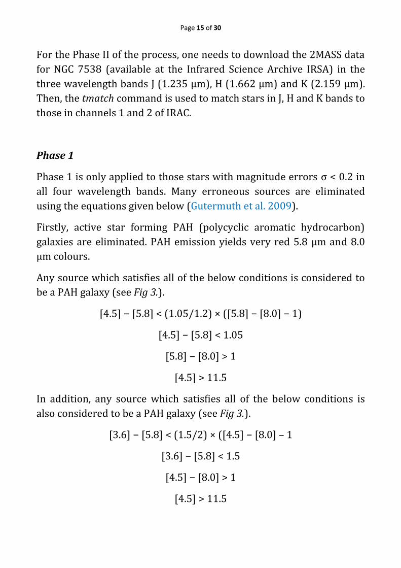
Firstly, active star forming PAH (polycyclic aromatic hydrocarbon)
galaxies are eliminated. PAH emission yields very red 5.8 µm and 8.0
µm colours.
Any source which satisfies all of the below conditions is considered to
be a PAH galaxy (see Fig 3.).
[4.5] − [5.8] < (1.05/1.2) × ([5.8] − [8.0] − 1)
[4.5] − [5.8] < 1.05
[5.8] − [8.0] > 1
[4.5] > 11.5
In addition, any source which satisfies all of the below conditions is
also considered to be a PAH galaxy (see Fig 3.).
[3.6] − [5.8] < (1.5/2) × ([4.5] − [8.0] – 1
[3.6] − [5.8] < 1.5
[4.5] − [8.0] > 1
[4.5] > 11.5
Page 16 of 30
Fig 3: Colour-Colour Diagram for the isolation of PAH galaxies.
Secondly, broad-line AGNs (Active Galactic Nuclei) are eliminated.
These AGNs are largely consistent with YSOs.
Any source which satisfies all of the below conditions is considered to
be an AGN (see Fig 4.).
[4.5] − [8.0] > 0.5
[4.5] > 13.5 + ([4.5] − [8.0] − 2.3)/0.4
[4.5] > 13.5
In addition, any source which satisfies any one of the below conditions
is also considered to be an AGN (see Fig 4.).
[4.5] > 14 + ([4.5] − [8.0] − 0.5)
[4.5] > 14.5 − ([4.5] − [8.0] − 1.2)/0.3
[4.5] > 14.5

Page 17 of 30
Fig 4: Colour-Magnitude Diagram for the isolation of broad-line AGNs.
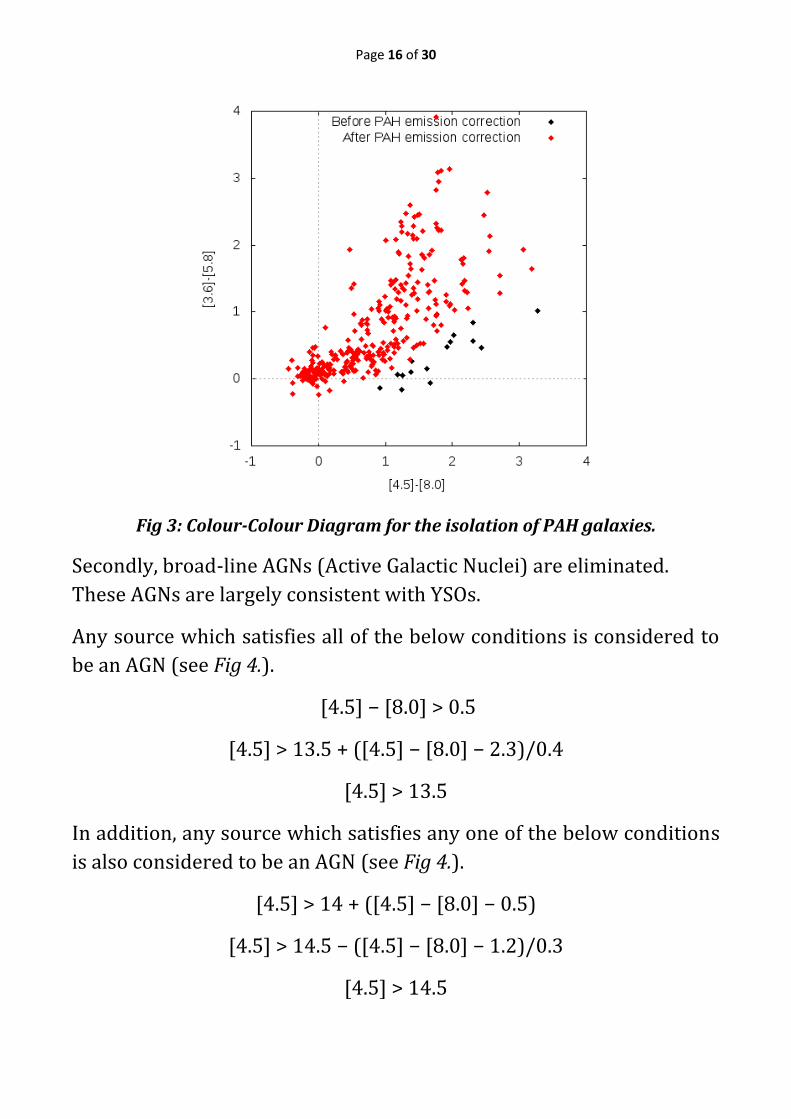
Thirdly, shock emission contamination must be eliminated. This is
detected in all four wavelength bands of IRAC.
Any source which satisfies all of the below conditions is considered to
be dominated by shock emission (see Fig 5.).
[3.6] − [4.5] > (1.2/0.55) × (([4.5] − [5.8]) − 0.3) + 0.8
[4.5] − [5.8] ≤ 0.85
[3.6] − [4.5] > 1.05
For other erroneous sources, we use the following sigma values. Each
is just the root-mean squared value of the errors in two bands.
σ1 = σ {[[4.5] − [5.8]]}
σ2 = σ {[[3.6] − [4.5]]}
Page 18 of 30
Fig 5: Colour-Colour Diagram for the isolation of sources contaminated by
shock emission.
σ3 = σ {[[4.5] − [8.0]]}
σ4 = σ {[[3.6] − [5.8]]}
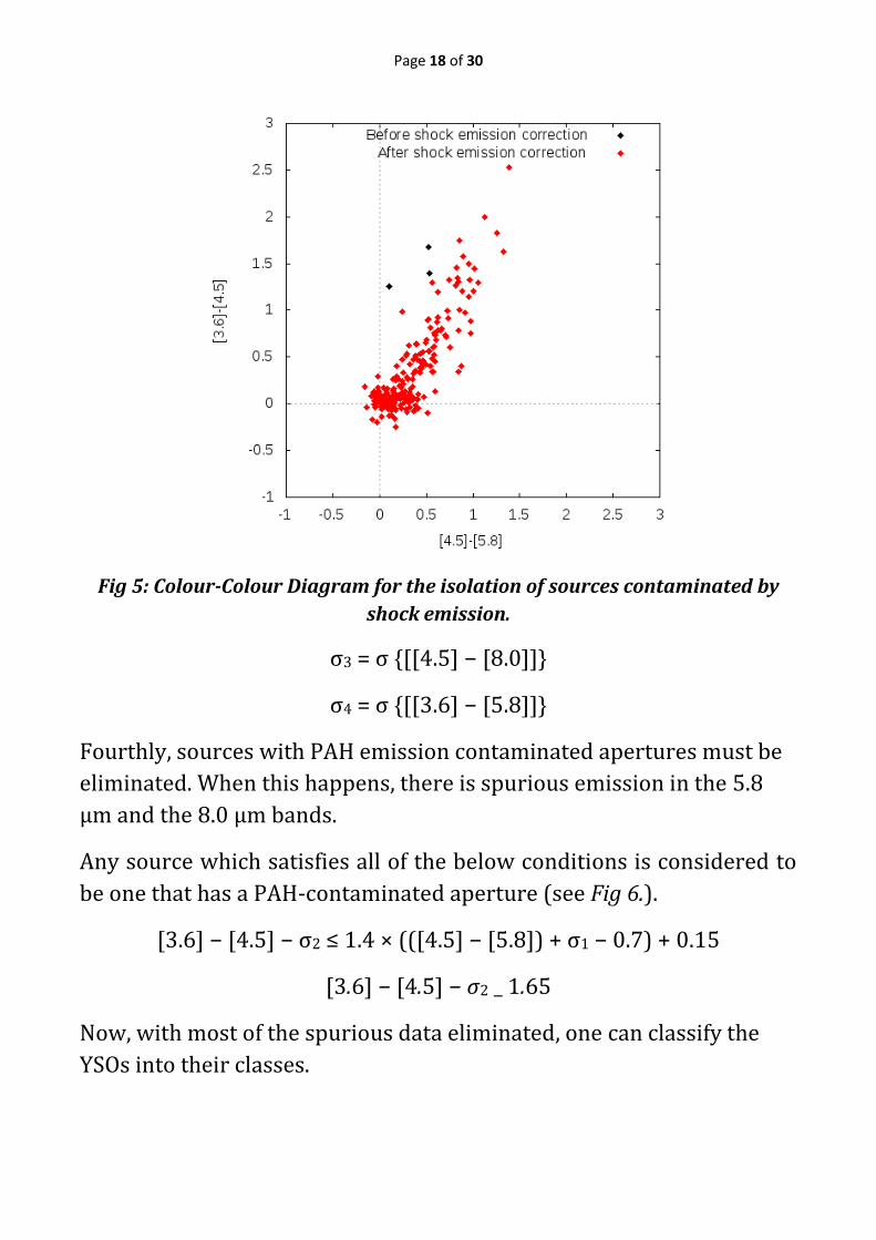
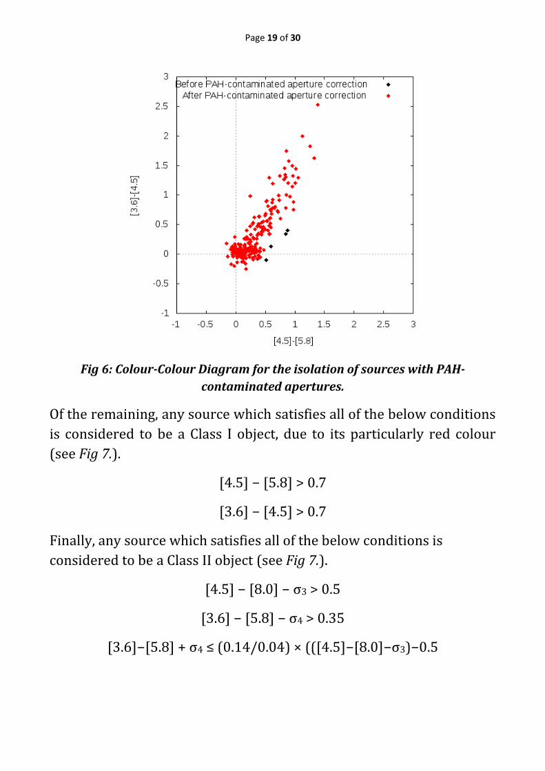
Fourthly, sources with PAH emission contaminated apertures must be
eliminated. When this happens, there is spurious emission in the 5.8
µm and the 8.0 µm bands.
Any source which satisfies all of the below conditions is considered to
be one that has a PAH-contaminated aperture (see Fig 6.).
[3.6] − [4.5] − σ2 ≤ 1.4 × (([4.5] − [5.8]) + σ1 − 0.7) + 0.15
[3.6] − [4.5] − σ2 _ 1.65
Now, with most of the spurious data eliminated, one can classify the
YSOs into their classes.
Page 19 of 30
Fig 6: Colour-Colour Diagram for the isolation of sources with PAH-
contaminated apertures.
Of the remaining, any source which satisfies all of the below conditions
is considered to be a Class I object, due to its particularly red colour
(see Fig 7.).
[4.5] − [5.8] > 0.7
[3.6] − [4.5] > 0.7
Finally, any source which satisfies all of the below conditions is
considered to be a Class II object (see Fig 7.).
[4.5] − [8.0] − σ3 > 0.5
[3.6] − [5.8] − σ4 > 0.35
[3.6]−[5.8] + σ4 ≤ (0.14/0.04) × (([4.5]−[8.0]−σ3)−0.5

Page 20 of 30
Fig 7: Colour-Colour Diagram showing Class I and Class II YSOs.
Phase 2
As mentioned before, the stars in the J, H and K bands of 2MASS and
channels 1 and 2 of IRAC are matched using the tmatch command
(same threshold of 3 arc seconds or 8.3333×10⁻⁴ degrees) of package
stsdas of IRAF. Phase II is applied only to those sources which lack
detection in channels 3 and 4, but have readings in the other five
wavelength bands. Furthermore, the process is carried out only for
those with magnitude errors σ < 0.2 in all bands (J, H, K, ch1, ch2).
Stars which have no detection (or null magnitude errors) in the J band,
but have detection in the K, H, ch1 and ch2 bands are also used in
Phase II. Now, these stars are filtered out based on their extinction
(colour excess) values. The ones used in this process are given below.
Page 21 of 30
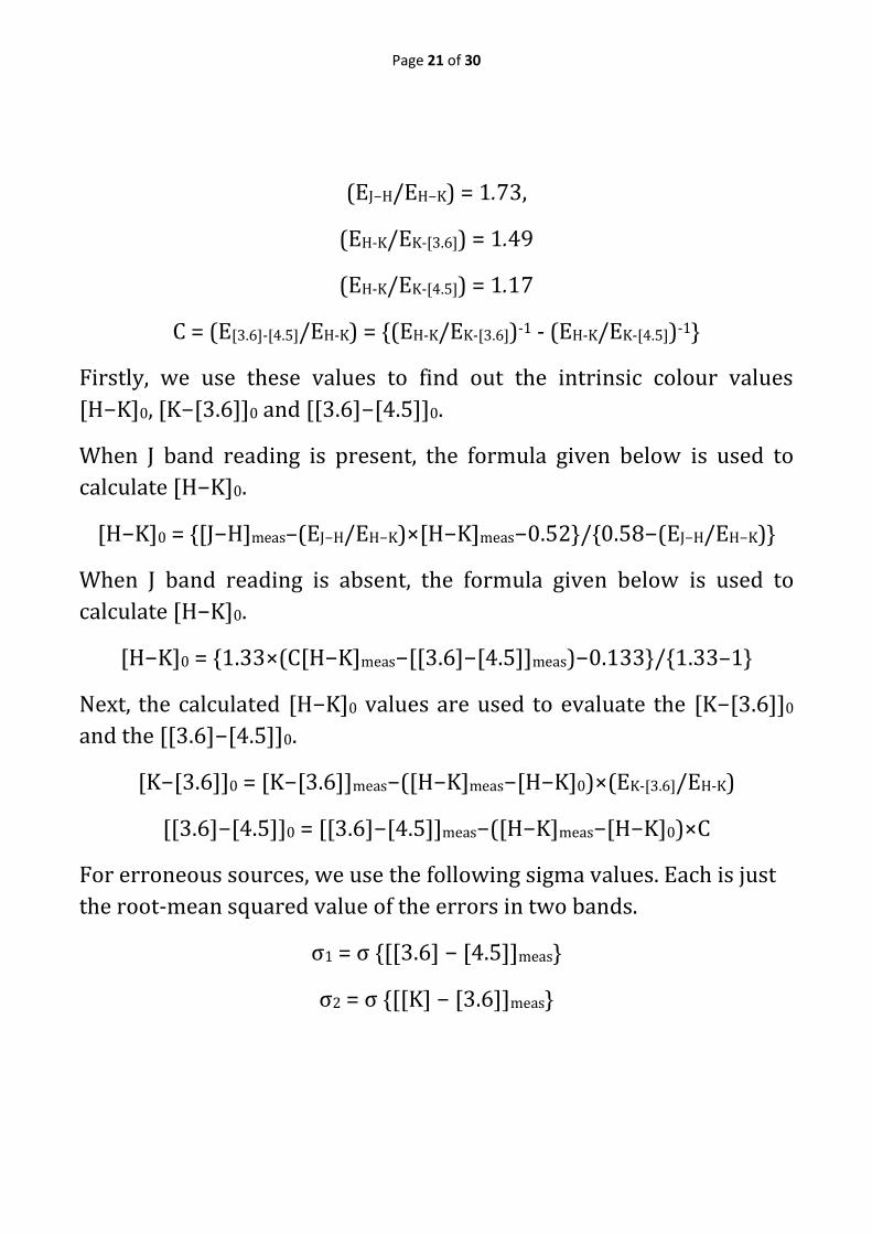
(EJ−H/EH−K) = 1.73,
(EH-K/EK-[3.6]) = 1.49
(EH-K/EK-[4.5]) = 1.17
C = (E[3.6]-[4.5]/EH-K) = {(EH-K/EK-[3.6])-1 - (EH-K/EK-[4.5])-1}
Firstly, we use these values to find out the intrinsic colour values
[H−K]0, [K−[3.6]]0 and [[3.6]−[4.5]]0.
When J band reading is present, the formula given below is used to
calculate [H−K]0.
[H−K]0 = {[J−H]meas–(EJ−H/EH−K)×[H−K]meas−0.52}/{0.58−(EJ−H/EH−K)}
When J band reading is absent, the formula given below is used to
calculate [H−K]0.
[H−K]0 = {1.33×(C[H−K]meas−[[3.6]−[4.5]]meas)−0.133}/{1.33–1}
Next, the calculated [H−K]0 values are used to evaluate the [K−[3.6]]0
and the [[3.6]−[4.5]]0.
[K−[3.6]]0 = [K−[3.6]]meas−([H−K]meas−[H−K]0)×(EK-[3.6]/EH-K)
[[3.6]−[4.5]]0 = [[3.6]−[4.5]]meas−([H−K]meas−[H−K]0)×C
For erroneous sources, we use the following sigma values. Each is just
the root-mean squared value of the errors in two bands.
σ1 = σ {[[3.6] − [4.5]]meas}
σ2 = σ {[[K] − [3.6]]meas}

Page 22 of 30
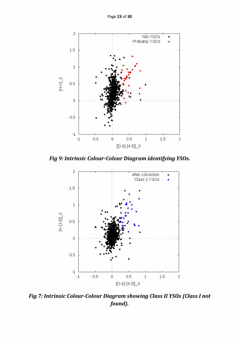
After this is done, classification begins. Additional YSO are those with
dereddened colours. Any source which satisfies all of the below
conditions is considered to be a YSO (see Fig 8. and Fig 9.).
[[3.6] − [4.5]]0 − σ1 > 0.101
[K − [3.6]]0 − σ2 > 0
[K − [3.6]]0 − σ2 > −2.85714 × ([[3.6] − [4.5]]0 − σ1 − 0.101) + 0.5
Fig 8: Colour-Colour Diagram identifying YSOs.
Also, any YSO which satisfies all of the below conditions is considered
to be a Class I object. The rest are considered Class II objects (see Fig
10.).
[K − [3.6]]0 − σ2 > − 2.85714 × ([[3.6] − [4.5]]0 − σ1 − 0.401) + 1.7
All sources classified as Class II objects must have [3.6] < 14.5 and
those classified as Class I objects must have [3.6] < 15.
Page 23 of 30
Fig 9: Intrinsic Colour-Colour Diagram identifying YSOs.
Fig 7: Intrinsic Colour-Colour Diagram showing Class II YSOs (Class I not
found).
Page 24 of 30
2.6 SED FITTING
The final part of this project involves fitting SEDs for YSOs and
extracting important parameters including ages and masses of
individual stars.
Before fitting the SEDs, the magnitudes of the YSOs must be converted
first to AB magnitudes, and then to spectral flux densities in mJy (milli-
jansky). This is necessary as the Python SED Fitter takes input only in
spectral flux densities in mJy.
[1 Jy = 10-26 W m-2 Hz-1]
AB magnitude is different from the regular magnitude in that it is
calibrated in absolute units of spectral flux densities (and not luminous
flux densities). Spectral flux density is the radiant flux density (SI unit
W m-2) per unit frequency.
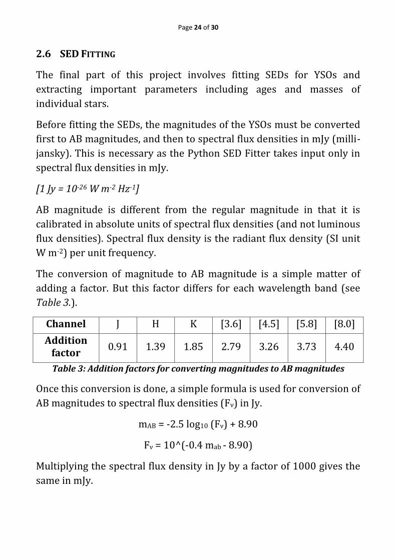
The conversion of magnitude to AB magnitude is a simple matter of
adding a factor. But this factor differs for each wavelength band (see
Table 3.).
Channel J H K [3.6] [4.5] [5.8] [8.0]
Addition factor
0.91 1.39 1.85 2.79 3.26 3.73 4.40
Table 3: Addition factors for converting magnitudes to AB magnitudes
Once this conversion is done, a simple formula is used for conversion of
AB magnitudes to spectral flux densities (Fν) in Jy.
mAB = -2.5 log10 (Fν) + 8.90
Fν = 10^(-0.4 mab - 8.90)
Multiplying the spectral flux density in Jy by a factor of 1000 gives the
same in mJy.
Page 25 of 30
Similarly, the magnitude errors (σm) must be converted to their
respective spectral flux density errors (σF).
σF = (Fν2 × σm) / 1.09
Next, an SED fitting model needs to be downloaded from the SED Fitter
website. In this project, the models_r06 is used as the fitting model.
Also, an extinction file kmh94.par must also be downloaded.
For a star to be fit using the SED fitter, it must have readings in at least
five of the seven wavelength bands (J, H, K, [3.6], [4.5], [5.8], [8.0]). If
not, the star is rejected. This new star list must be edited to a particular
format which can be inputted to the SED Fitter program. The format of
24 columns is given below.
ID RA Dec PJ PH PK P1 P2 P3 P4 mJ σJ mH σH
mK σK m1 σ1 m2 σ2 m3 σ3 m4 σ4
In the above format, the P-columns take the value 0 (if data in that
band is absent) or 1 (if data in that band is present), the m-columns are
the spectral flux density values in mJy and the σ-columns are the
spectral flux density errors in mJy. The subscripts 1, 2, 3 and 4 denote
[3.6], [4.5], [5.8] and [8.0] wavelength bands respectively.
Out of all the YSOs isolated from Phase I and Phase II classification,
only 23 of them (3 Class I objects and 20 Class II objects) were found to
have data in all seven bands (J, H, K, [3.6], [4.5], [5.8], [8.0]), and 21 of
them (all Class II objects) were found to have data in five bands (J, H, K,
[3.6], [4.5]).
Finally, a Python fit.py file is written, with the inputs as described
above. The code used is written below.
from astropy import units as u
from sedfitter import fit
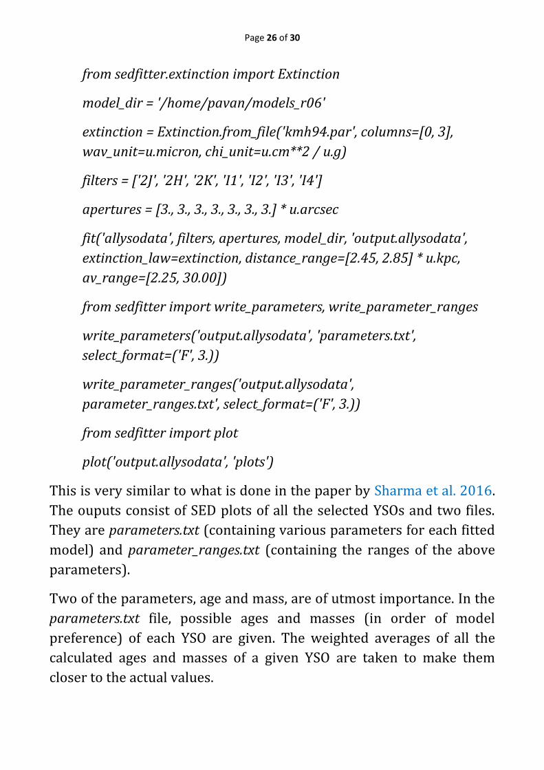
Page 26 of 30
from sedfitter.extinction import Extinction
model_dir = '/home/pavan/models_r06'
extinction = Extinction.from_file('kmh94.par', columns=[0, 3],
wav_unit=u.micron, chi_unit=u.cm**2 / u.g)
filters = ['2J', '2H', '2K', 'I1', 'I2', 'I3', 'I4']
apertures = [3., 3., 3., 3., 3., 3., 3.] * u.arcsec
fit('allysodata', filters, apertures, model_dir, 'output.allysodata',
extinction_law=extinction, distance_range=[2.45, 2.85] * u.kpc,
av_range=[2.25, 30.00])
from sedfitter import write_parameters, write_parameter_ranges
write_parameters('output.allysodata', 'parameters.txt',
select_format=('F', 3.))
write_parameter_ranges('output.allysodata',
parameter_ranges.txt', select_format=('F', 3.))
from sedfitter import plot
plot('output.allysodata', 'plots')
This is very similar to what is done in the paper by Sharma et al. 2016.
The ouputs consist of SED plots of all the selected YSOs and two files.
They are parameters.txt (containing various parameters for each fitted
model) and parameter_ranges.txt (containing the ranges of the above
parameters).
Two of the parameters, age and mass, are of utmost importance. In the
parameters.txt file, possible ages and masses (in order of model
preference) of each YSO are given. The weighted averages of all the
calculated ages and masses of a given YSO are taken to make them
closer to the actual values.
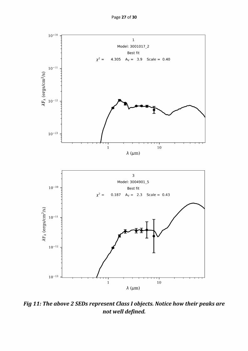
Page 27 of 30
Fig 11: The above 2 SEDs represent Class I objects. Notice how their peaks are
not well defined.
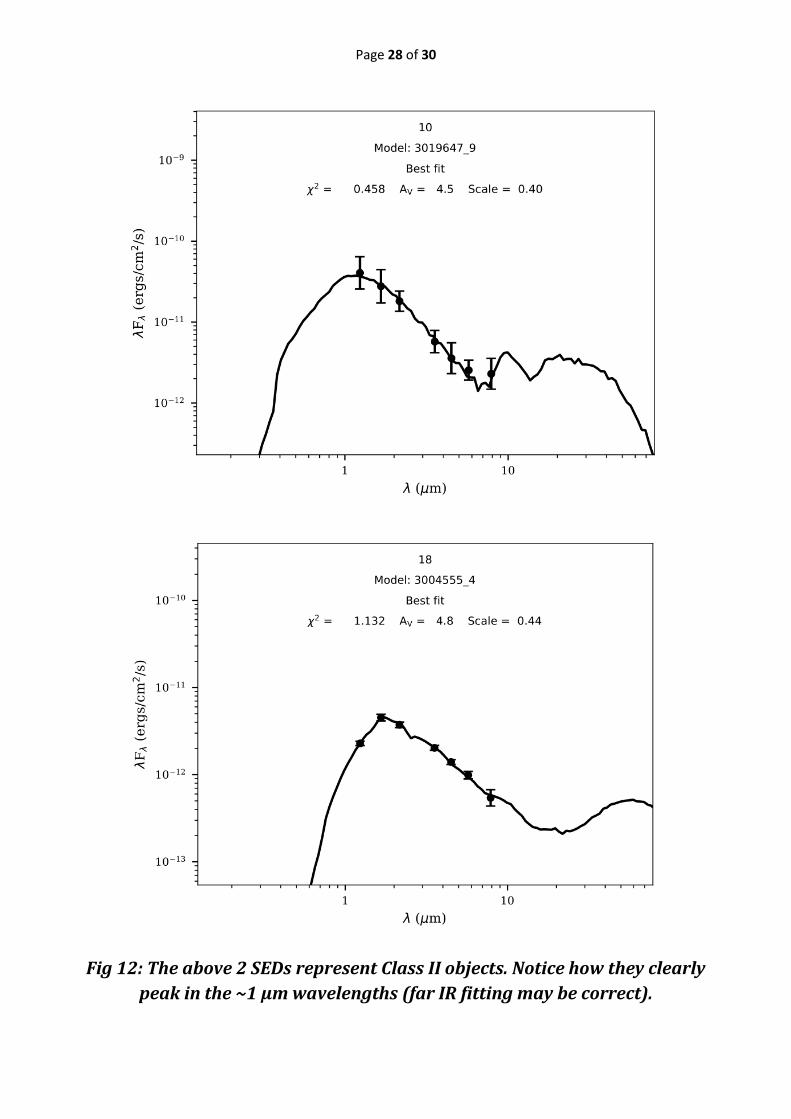
Page 28 of 30
Fig 12: The above 2 SEDs represent Class II objects. Notice how they clearly
peak in the ~1 µm wavelengths (far IR fitting may be correct).
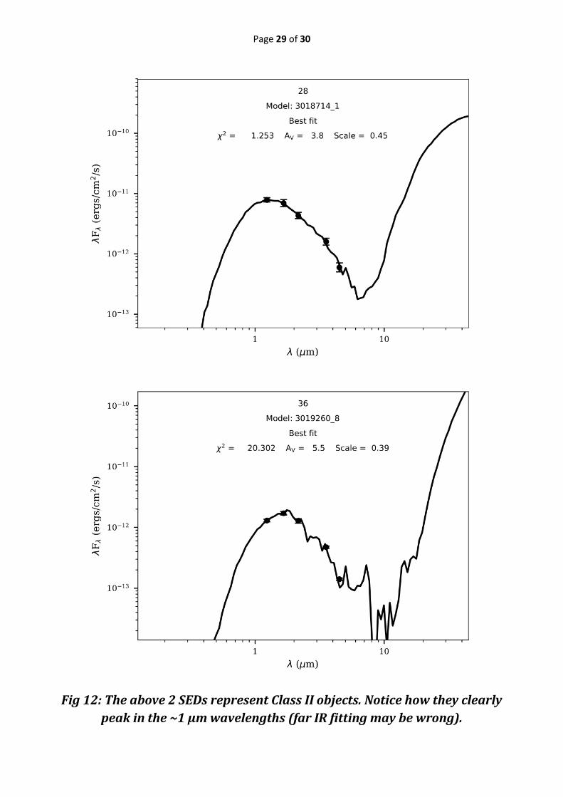
Page 29 of 30
Fig 12: The above 2 SEDs represent Class II objects. Notice how they clearly
peak in the ~1 µm wavelengths (far IR fitting may be wrong).
Page 30 of 30
2.7 RESULTS
Spitzer data for NGC 7538 was mosaicked using MOPEX (for all four
channels). Photometry was conducted on these mosaic images, and
various star parameters were found.
YSOs were isolated I two phases. In phases I and II, 27 and 0 Class I
objects, and 42 and 33 Class II objects were identified respectively.
Finally, SEDs for 44 (3 Class I objects and 41 Class II objects) of these
YSOs were fitted, confirming that they were indeed Class I and Class II
objects, and the masses and ages of individual YSOs were calculated
using weighted averages. Fitting would have been more accurate had
there been far IR (MIPS) data too.
3 ACKNOWLEDGEMENTS
First, I would like to thank my mentor and supervisor, Dr. Saurabh
Sharma for his guidance and for giving me very exciting work to do. I
learnt a lot about Star Formation and various data
reduction/photometry techniques through my project.
I am grateful to LINUX Ubuntu and its super-helpful commands, awk
being the most prominent, although many others have helped me
numerous times.
I am thankful for the climate at ARIES Nainital, which was pleasant
(unlike most other places during Summer) enough to let me do my
work in peace and comfort.
Lastly, I would like to thank all my friends here for not being boring,
my friends away for being in touch and my family for their
encouragement.
Thank you.