Policy Research Working Paper 5954

Identification of Sources of Variation in Poverty Outcomes

B. Essama-Nssah

The World BankPoverty Reduction and Economic Management Network

January 2012

WPS5954P

ublic

Dis

clos

ure

Aut

horiz

edP

ublic

Dis

clos

ure

Aut

horiz

edP

ublic

Dis

clos

ure

Aut

horiz

edP

ublic

Dis

clos

ure

Aut

horiz

edP

ublic

Dis

clos

ure

Aut

horiz

edP

ublic

Dis

clos

ure

Aut

horiz

edP

ublic

Dis

clos

ure

Aut

horiz

edP

ublic

Dis

clos

ure

Aut

horiz

ed

Produced by the Research Support Team

Abstract

The Policy Research Working Paper Series disseminates the findings of work in progress to encourage the exchange of ideas about development issues. An objective of the series is to get the findings out quickly, even if the presentations are less than fully polished. The papers carry the names of the authors and should be cited accordingly. The findings, interpretations, and conclusions expressed in this paper are entirely those of the authors. They do not necessarily represent the views of the International Bank for Reconstruction and Development/World Bank and its affiliated organizations, or those of the Executive Directors of the World Bank or the governments they represent.

Policy Research Working Paper 5954

The international community has declared poverty reduction one of the fundamental objectives of development, and therefore a metric for assessing the effectiveness of development interventions. This creates the need for a sound understanding of the fundamental factors that account for observed variations in poverty outcomes either over time or across space. Consistent with the view that such an understanding entails deeper micro empirical work on growth and distributional change, this paper reviews existing decomposition methods that can be used to identify sources of variation in poverty. The maintained hypothesis is that

This paper is a product of the Poverty Reduction and Equity Group, Poverty Reduction and Economic Management Network. It is part of a larger effort by the World Bank to provide open access to its research and make a contribution to development policy discussions around the world. Policy Research Working Papers are also posted on the Web at http://econ.worldbank.org. The author may be contacted at essama.nssah@gmail.com.

the living standard of an individual is a pay-off from her participation in the life of society. In that sense, individual outcomes depend on endowments, behavior and the circumstances that determine the returns to those endowments in any social transaction. To identify the contribution of each of these factors to changes in poverty, the statistical and structural methods reviewed in this paper all rely on the notion of ceteris paribus variation. This entails the comparison of an observed outcome distribution to a counterfactual obtained by changing one factor at a time while holding all the other factors constant.

Identification of Sources of Variation in Poverty Outcomes

B. Essama-Nssah

Poverty Reduction and Equity Group

The World Bank

Washington D.C.

Keywords: Counterfactual analysis, distribution, endowment effect, identification,

inequality, Oaxaca-Blinder decomposition, poverty, social evaluation, structural effect,

treatment effect.

JEL Codes: C14, C15, C31, D31, I32

The author is grateful to Francisco H. G. Ferreira, Gabriela Inchauste and Emmanuel Skoufias for useful comments and suggestions on an earlier version of this paper. The views expressed herein are entirely those of the author or the literature cited and should not be attributed to the World Bank or to its affiliated organizations.

2

1. Introduction

Poverty reduction is one of the key objectives of socioeconomic development. The

first World Development Report (WDR) argued that development efforts should be aimed

at the twin objectives of rapid growth and poverty reduction1 (World Bank 1978). This

vision of development has been reiterated in one form or another in subsequent reports

culminating in a conception of development as opportunity equalization presented in WDR

2006 (World Bank 2005). In this context, equity is defined in terms of a level playing field

where individuals have equal opportunities to pursue freely chosen life plans and are

spared from extreme deprivation in outcomes. In this sense, the pursuit of equity also

entails that of poverty reduction.

A recent review of poverty trends across the world has shown that poverty had

been on a steady decline for a wide variety of countries from the late 1990s up until 2009

(when the financial crisis hit the world economy). The evidence on inequality reduction, a

key determinant of poverty outcomes, is however mixed. From the policymaking

perspective, it is important to understand the factors driving these observed outcomes.

Focusing on the fact that distributional statistics are computed on the basis of a

distribution of the living standards which is fully characterized by its mean and the degree

of inequality, several authors have proposed counterfactual decomposition methods to

identify the contribution of changes in the mean and in inequality to variations in overall

poverty. These decompositions include the Datt-Ravallion (1992) method, which splits the

change in poverty into distribution-neutral growth effect, a redistributive effect and a

residual interpreted as an interaction term. The Shapley method proposed by Shorrocks

(1999) is analogous to that of Datt and Ravallion, but does not involve a residual. Kakwani

(2000) has proposed an equivalent approach. Ravallion and Huppi (1991) offer a way of

decomposing change in poverty over time into intrasectoral effects, a component due to

population shifts and an interaction term between sectoral changes and population shifts.

We present a detailed review of all these macro methods in the appendix. 1 This recommendation is consistent with the theme underlying the study of redistribution with growth by Chenery

et al. (1974). This study advocates the use of explicit social objectives as a basis for choosing development policies

and programs. In particular, any development intervention must be evaluated in terms of the benefits it provides to

different socio-economic groups.

3

However, the usefulness of the above described decomposition methods in

policymaking is severely limited by the fact that they explain changes in poverty on the

basis of changes in summary statistics that are hard to target with policy instruments. The

difficulty stems from the fact that such statistics hide more than they reveal about the

heterogeneity of impacts underlying aggregate outcomes. It is well known that

heterogeneity of interests and of individual circumstances plays a central role in both

policymaking and in the determination of the welfare impact of policy. Ravallion (2001)

argues that understanding this heterogeneity is crucial for the design and implementation

of targeted interventions that might enhance the effectiveness of growth-oriented policies.

He further adds that such an understanding must stem from a deeper micro empirical work

on growth and distributional change.

The purpose of this paper is to review the essence of existing methods that can be

used to identify key factors that drive changes in the observed poverty outcomes. The

paper is akin to the excellent review by Ferreira (2010) of the evolution of the

methodology for understanding the determinants of the relationship between economic

growth, change in inequality and change in poverty. While that review covers the macro-,

meso- and micro-economic approaches, we focus on a variety of micro-decomposition

methods and delve deeper into the identification strategy underlying each of these

methods. The point of departure of these methods is the same as that of the macro

methods noted above and presented in the appendix. They too start from the fact that

poverty measures, along with many other distributional statistics, can be viewed as real-

valued functionals of the relevant distributions2 so that changes in poverty are due to

changes in the underlying distribution of living standards. Macro-decomposition methods

proceed by characterizing changes in the underlying distribution in terms of changes in

aggregate statistics such as the mean, relative inequality, sub-group population shares and

within-group poverty. The micro-decomposition methods reviewed here go beyond these

summary statistics and attempt to link distributional changes to fundamental elements that

drive these changes.

2 Roughly speaking, a functional is a function of a function. In this particular context, it is a rule that maps every distribution in its domain into a real number (Wilcox 2005).

4

The outline of the paper is as follows. Section 2 presents the basic framework

underlying all decomposition methods considered in this paper. The logic underpinning all

these methods can be organized around the following terms: (i) domain, (ii) outcome

model, (iii) scope, (iv) identification, and (v) estimation. The type of distributional change

a method seeks to decompose on the basis of a model that links the outcome of interest to

its determining factors defines the domain of that method. The specification of the outcome

model associated with a decomposition method determines the potential scope of the

method, where scope represents the set of explanatory factors the method tries to uncover

by decomposition. In other words, the scope defines the terms of the decomposition.

Identification concerns the assumptions needed to recover, in a meaningful way, various

terms of the decomposition. The outcome model is used to construct counterfactuals on

the basis of ceteris paribus variations of the determinants in order to identify the

contribution of each such factor to observed changes in the object of interest. Finally,

estimation involves the computation of identified parameters on the basis of sample data.

These ideas, which constitute in fact the methodological bedrock of impact evaluation, will

be illustrated within the basic Oaxaca-Blinder framework for decomposing changes in the

mean of a distribution, and its generalization to any distributional statistic.

Section 3 reviews methods used to identify and estimate the endowment and price

effects along the entire outcome distribution. Decomposing changes in whole distributions

of outcomes is bound to reveal heterogeneity in the impact of the growth or development

process on economic welfare. Furthermore, a poverty-focused analysis requires an

understanding of what goes on at and below the poverty line. This section will therefore

focus on the decomposition of differences in density functions and across quantiles based

on purely statistical methods that rely on conditional outcome distributions. It discusses

the residual imputation method proposed by Juhn, Murphy and Pierce (1993) to split the

price effect into a component due uniquely to observable characteristics and another due

to unobservables. One particular advantage of the statistical approach is that it provides

the analyst with semi- and non-parametric methods for the identification of the aggregate

endowment and price effects without having to impose a functional form on the

relationship between the outcome and its determinants. However, the statistical

5

framework is unable to shed light on the mechanism underlying that relationship. The

decomposition results therefore do not have any causal interpretation.

Bourguignon and Ferreira (2005) note that, in addition to the endowment and price

effects, long-run changes in the distribution of the living standards are driven by changes in

agents’ behavior with respect to labor supply, consumption patterns, or fertility choice. A

key limitation of the methods reviewed in section 3 is that they fail to account for the effect

of behavioral changes in addition to the composition and structural effects. Because these

methods are based on statistical models of conditional distributions, it is conceivable that

the behavioral effect is mixed up with the price effect identified by these methods. Section

4 therefore considers methods that have been proposed to account for behavioral

responses to changes in the socioeconomic environment. All these methods rely on the

specification and estimation of a microeconometric model based on some theory of

individual (or household) behavior and social interaction. These methods go a step further

in trying to identify factors associated with structural elements that underpin observed

changes in poverty outcomes. Both the statistical and structural approaches seek to model

conditional outcome distributions. A key distinction between the two approaches is that

the former relies entirely on statistics while the later combines economics and statistics.

While the methods reviewed here have been applied mostly in labor economics to

decompose wage distributions, this review will pay special attention to their adaptability to

the decomposition of household consumption which is the basis of poverty measurement.

Consideration will also be given to model specifications that drop the assumption of

perfectly competitive markets to accommodate situations found most frequently in rural

areas in developing countries. Concluding remarks are made in section 5.

2. The Basic Framework

This section presents a theory of counterfactual decomposition of variations in

individual and social outcomes and illustrates that conceptual framework in the context of

the classic Oaxaca-Blinder method and its generalization to the case of a generic

distributional statistic.

6

2.1. A Theory of Counterfactual Decomposition

All decomposition methods considered in this paper (including the macro methods

presented in the appendix) are governed by a basic theory of counterfactual

decomposition. Each method can be characterized in terms of the following elements:

domain, outcome model, scope, identification and estimation procedure. The domain is the

type of distributional changes the method seeks to decompose (e.g. changes in poverty over

time or across space). The outcome model links the outcome of interest to its determining

factors. A poverty measure, for instance, is a social outcome that is a functional of the

underlying distribution of individual outcomes. As noted in the introduction and

demonstrated in the appendix, macro-decomposition methods use this fact to link

variations in poverty to changes in the mean and relative inequality characterizing the

underlying distribution.

Outcome models used by micro-decomposition methods can be motivated as

follows. Poverty measurement is based on a distribution of living standards. The living

standard of an individual is an outcome of an interaction between opportunities offered by

society and the ability of the individual to identify and exploit such opportunities. In other

words, the living standard of an individual is a pay-off from her participation in the life of

society. One can thus think of life in society as a game defined by a set of rules governing

various interactions of the parties involved (players). These rules spell out what the

concerned parties are allowed to do and how these allowable actions determine outcomes.

An environment within which a game is played consists of three basic elements: (1) a set of

potential participants, (2) a set of possible outcomes and (3) a set of possible types of

participants (players). Types are characterized by their preferences, capabilities,

information and beliefs (Milgrom 2004). The operation of a game can be represented by a

function mapping environments to potential outcomes. Thus an individual pay-off is a

function of participation and type. This paradigm motivates our thinking of the living

standard of an individual as a function of endowments, behavior and the circumstances that

determine the returns to these endowments from any social transaction.

7

The outcome model can take the form of a single equation or a set of equations (as

we will see in section 4) and ultimately establishes a relationship between the domain and

the scope of the decomposition method. The scope is the set of explanatory factors the

method tries to uncover by decomposition. In fact, the specification of the outcome model

determines the potential scope of the corresponding decomposition method. For instance,

the scope of the macro methods reviewed in the appendix is limited to some aggregate

statistics based on the underlying outcome distribution. Such statistics include: the mean,

measures of relative inequality, population shares and within-group poverty. The outcome

model underlying micro-decomposition methods implies that the potential scope for these

methods includes endowment and price effects, and behavioral responses. However, the

statistical methods discussed in section 3 are unable to account for behavior because they

are based only on the joint distribution of the outcome and individual characteristics.

Methods reviewed in section 4 can account for behavioral responses in addition to the

endowment and price effects. This ability stems from the fact that these methods combine

economic theory of behavior and social interaction with statistics to explain observed

outcomes. Behavior, endowments and prices thus represent some of the deep structural

elements that drive the distributional changes underlying observed variations in poverty

outcomes.

Identification concerns the assumptions needed to recover the factors of interest at

the population level. While macro- and micro-decomposition methods differ in their scope

(meaning the elements they try to identify) they share the same fundamental identification

strategy based on the notion of ceteris paribus variation. Attribution of outcomes to policy

is the hallmark of policy impact evaluation. Indeed, variations in individual outcomes

associated with the implementation of a policy are not necessarily due to the policy in

question. These variations could be driven by changes in confounding factors in the

socioeconomic environment. At the most fundamental level, all identification strategies

seek to isolate an independent source of variation in policy and link it to the outcome of

interest to ascertain impact. Macro and micro methods base identification of the

determinants of differences across distributions of living standards on a comparison of

counterfactual distributions with the observed ones. Counterfactual distributions are

8

obtained by changing one determining factor at a time while holding all the other factors

fixed (this is a straight application of the notion of ceteris paribus variation).

Estimation involves the computation of the relevant parameters on the basis of

sample data. The linchpin of the whole process is the estimation of credible

counterfactuals. In the context of micro-decomposition methods, there is a key

counterfactual that must be carefully estimated, namely: the distribution of outcomes in the

base state (t=0) assuming the distribution of individual characteristics prevailing in the end

state (t=1). Put another way, that counterfactual represents the distribution of outcomes

that would prevail in the end state if the characteristics in that state had been treated

according to the outcome structure prevailing in the initial state. Depending on the chosen

functional form for the outcome equation, there are both parametric and nonparametric

ways of estimating this counterfactual. We now consider the translation of these basic

ideas into the Oaxaca-Blinder decomposition framework.

2.2. The Classic Oaxaca-Blinder Method

Structure

As discussed in the next subsection, micro-decomposition methods encountered in

the literature may be considered a generalization of the classic Oaxaca-Blinder

decomposition method. This approach assumes that the outcome variable y is a linear

function of individual characteristics that is also separable in observable covariates x and

unobservable factors ε. In addition, it is assumed that the conditional mean of ε given the

observables is equal to zero. Focusing on variations over time, we let t=0 for the initial

period and 1 for the end period. Then the relationship between y and its determinants can

be written as follows.

(1)

Abstracting from the time subscript, the conditional mean outcome can be written as

follows: Therefore β is a measure of the effect of x on the conditional mean

outcome. Furthermore, the law of iterated expectations implies that the unconditional

mean outcome is: This result implies that β also measures the

9

effect of changing the mean value of x on the unconditional mean value of y. This is the

interpretation underlying the original Oaxaca-Blinder decomposition (Fortin, Lemieux and

Firpo 2011).

Let represent the overall difference in unconditional mean

outcome between the two periods. This is the domain of the classic Oaxaca-Blinder

method. This domain can also be expressed as: . The average

outcome for period 1 valued on the basis of the parameters for period 0 is equal to .

This is a counterfactual outcome for period 1. We can subtract it from and add it back to

the above overall mean difference to get the following expression3.

(2)

Looking at the regression coefficients β as characterizing the returns to (or reward for)

observables characteristics, this aggregate decomposition reveals that, under the

maintained assumptions (i.e. identifying assumptions), the overall mean difference can be

expressed as:

, where

is the endowment effect and

is the price effect4.

The assumption of additive linearity implies that one can also perform a detailed

decomposition whereby the endowment and price effects are each divided into the

respective contribution of each covariate. To see this formally, let xk and βk stand

respectively for the kth

element of x and β. Then the endowment and price effects can be written

in terms of sums over the explanatory variables. For the endowment effect, we have

(3)

Similarly for the structural effect, we have the following expression

(4)

3 An alternative expression is based on this counterfactual: . The corresponding decomposition is:

.

4 In the literature, the endowment effect is also known as the composition effect while the price effect is also referred to as the structural effect. See Fortin, Lemieux and Firpo (2011) for the use of this terminology.

10

Expressions (3) and (4) provide a simple way of dividing the endowment and the price effects

into the contribution of a single covariate or a group of covariates as needed.

The above components are easily computed by replacing the expected values by the

corresponding sample means and the coefficients associated with the covariates by their OLS

estimates. An estimate of the endowment effect is:

(5)

Similarly, for the price effect, we have the following expression.

(6)

Interpretation

As Fortin, Lemieux and Firpo (2011) point out, there is a powerful analogy between

the Oaxaca-Blinder decomposition method and treatment effect analysis5. Treatment

impact analysis seeks to identify and estimate the average effect of treatment (i.e.

intervention) on the treated (i.e. those exposed to an intervention) on the basis of the

difference in average outcomes between the treated and a comparison group. In that

context, t indicates treatment status. It is equal to 1 for the treated and 0 for the untreated

(the comparison or control group). The expression, , can therefore be

interpreted as the difference in average outcomes between the treated and untreated.

Under the assumptions6 underlying the basic Oaxaca-Blinder method, it is clear that this

difference is due to differences in observable characteristics (i.e. the composition effect)

and in treatment status. The part due to the difference in treatment status is known as the

5 Indeed, these authors provide a systematic interpretation of decomposition methods within the logic of program impact evaluation. 6 According to Fortin, Lemieux and Firpo (2011), these assumptions include the following: (1)Mutually exclusive groups;(2) The outcome structure is an additively separable function of characteristics; (3) Zero conditional mean for unobservables given observed characteristics;(4)Common support for the distributions of characteristics across groups (to rule out cases where arguments of the outcome function may differ across groups; (5) Simple counterfactual treatment, meaning that the outcome structure of one group is assumed to be a counterfactual for the other group. This last assumption rules out general equilibrium effects so that observed outcomes for one group or time period can be reasonably used to construct counterfactuals for the other group or time period. The Oaxaca-Blinder method therefore follows a partial equilibrium approach.

11

average treatment effect on the treated (ATET) and is in fact equal to the structural or price

effect.

Note that the conventional approach to impact evaluation also relies on ceteris

paribus variation of treatment in order to identify its average effect on the treated. Within

that logic, the composition effect is equivalent to selection bias that must be driven to zero

by the use of randomization, propensity score matching or similar methods.

Randomization ensures that the distribution of observed and unobserved characteristics is

the same for both the treated and the control group. By balancing observed and

unobserved characteristics between the groups prior to the administration of treatment,

randomization guarantees that the average difference in outcome between the two groups

is due to treatment alone, hence the causal interpretation given to this parameter under

those circumstances. In other words, the first term on the right hand side of equation (2),

that is the endowment effect or selection bias, is equal to zero under random assignment to

treatment and full compliance7. It is clear that randomization is designed to implement a

ceteris paribus variation in treatment.

In the context of observational studies where the investigator does not have control

over the assignment of subjects to treatment, the determination of the causal effect of

treatment hinges critically on the understanding of the underlying treatment assignment or

selection mechanism which must explain how people end up in alternative treatment states.

The assumption of selection on observables (also known as ignorability) is often invoked to

implement ceteris paribus identification of the average treatment effect through

conditioning by stratification. Basically, conditioning by stratification entails comparing

only those subjects with the same value of covariates x across the two groups (treated and

untreated). This type of selection of individuals from the two groups is known as matching.

7 Heckman and Smith (1995) explain that the mean outcome of the control group provides an acceptable estimate of the counterfactual mean if randomization does not alter the pool of participants or their behavior, and if no close substitutes for the experimental program are readily available. These authors further note that randomization does not eliminate selection bias, but rather balances it between the two samples (participants and nonparticipants) so that it cancels out when computing mean impact. There would be randomization bias if those who participate in an experiment differ from those who would have participated in the absence of randomization. Furthermore, substitution bias would occur if members of the control group can easily obtain elsewhere close substitutes for the treatment.

12

There is a potential dimension problem associated with matching when there are many

observable characteristics taking many values. Insisting on conditioning based on exact

values can lead to too few observations in each subgroup characterized by these

observables. This dimensionality problem can be resolved by matching on the propensity

score, that is, the conditional probability of receiving treatment given observable

characteristics (Rosenbaum and Rubin 1983).

The analogy between treatment effect analysis and the Oaxaca-Blinder

decomposition method has been extremely useful for the development of flexible

estimation methods for endowment and structural effects. Fortin, Lemieux and Firpo

(2011) explain that selection on observables implies that the conditional distribution of

unobservable factors is the same in both groups (treated and comparison). They further

note that, while this assumption is weaker than the zero conditional mean assumption8

used in the standard Oaxaca-Blinder decomposition, it is enough to secure identification

and consistent estimation of the ATET and hence the structural effect,

, (in the Oaxaca-

Blinder framework). These authors give the example of education and unobservable

ability. They explain that if education and ability are correlated, this creates an

endogeneity problem that prevents a linear regression of earnings on education to produce

consistent estimates of the structural parameters measuring the return to education. Yet

the aggregate decomposition remains valid as long as the correlation between ability and

education is the same in both groups.

A major implication of the difference in identification assumptions between the

traditional Oaxaca-Blinder approach and treatment effect analysis is that consistent

estimators of the ATET such as inverse probability weighing (IPW) and matching can be

used to estimate the structural effect (

) even if the underlying relationship between the

outcome and covariates is not linear. Given such an estimate, the composition effect can be

calculated as a residual from the overall mean difference as follows:

. In

8 Recall that, the identification of the two components of the aggregate Oaxaca-Blinder decomposition relies on the zero conditional mean assumption for the unobservable factors stated as: . This condition is what allows the analyst to claim that on average, variation in x is unrelated to variation in the unobservables, a manifestation of ceteris paribus variation.

13

particular, decomposition methods based on this weighting procedure are known to be

efficient.

Limitations

While treatment effect analysis can help with the identification and estimation of the

structural effect, it is important to note that there are two basic reasons why this effect

does not necessarily inherit the causal interpretation generally enjoyed by the ATET. The

first reason stems from the fact that in many cases, group membership is not the result of a

choice or an exogenous assignment but a consequence of an intrinsic characteristic such as

gender or race. The other important reason is that many of the observable covariates are

not equivalent to the so-called pre-treatment variables that are not supposed to be affected

by the treatment (Fortin, Lemieux and Firpo 2011).

Fortin, Lemieux and Firpo (2011) point out two other important limitations of the

standard Oaxaca-Blinder decomposition method. The contribution of each covariate to the

structural effect is highly sensitive to the choice of the omitted group when the explanatory

variables include a categorical variable. Jann (2008) discusses possible solutions to this

problem. The second limitation stems from the fact that the decomposition provides

consistent estimates only under the assumption that the conditional expectation is linear.

Under the linearity assumption, the counterfactual average when t=1 is simply equal

to: This is estimated by the cross-product of sample means of

characteristics for t=1 with the relevant OLS coefficients from t=0. The corresponding

estimate is: . The counterfactual mean outcome will not be equal to this term when

linearity does not hold. One possible solution is to reweight the sample for t=0 using the

inverse probability method9 and to compute the counterfactual mean outcome on the basis

of statistics from the reweighted counterfactual sample. Let be the vector of the means

of adjusted covariates in t=0, and the corresponding least squares coefficients. Then the

correct counterfactual mean outcome when the linearity assumption does not hold is:

.

This is the term to add to and subtract from the empirical version of the overall difference

9 We will come back to this point in the next subsection.

14

in mean outcome to get the appropriate estimates of the endowment and structural effects

when the linearity assumption fails.

2.3. A Generalization of the Oaxaca-Blinder Decomposition

As noted above, the standard Oaxaca-Blinder decomposition method focuses on

differences in mean outcomes between two groups and relies on some stringent

assumptions to identify the endowment and structural effects. We now consider how to

extend the logic underlying this method to the decomposition of differences in

distributional statistics other than the mean such as poverty or inequality measures. We

consider both aggregate and detailed decompositions.

Aggregate Decomposition

Just as in the case of the basic Oaxaca-Blinder method, we are interested in

decomposing a change in some distributional statistic, say θ, from the base period t=0 to

the end period t=1. As noted in the introduction, all distributional statistics such as the

mean, quantiles, the variance, poverty and inequality measures, can be viewed as

functionals of the underlying outcome distribution. Thus, the principle of decomposition

presented here applies to all of them. Let stand for the outcome distribution

observed in the initial period and that observed in the final period. The overall

difference in the distribution of outcomes between states 0 and 1 can be written in terms of

θ(F) as follows (Fortin, Lemieux and Firpo 2011).

(7)

Equation (7) characterizes the domain of the decomposition methods in this paper.

As far as the scope is concerned, most micro methods seek to decompose this overall

difference on the basis of the relationship between the outcome variable and individual or

household characteristics. The following equation represents a general expression of that

relationship.

. (8)

15

Equation (8) suggests that conditional on the observable characteristics, x, the

outcome distribution depends only on the function φt(∙) and the distribution of the

unobservable characteristics ε. Thus there are four potential terms in the scope of micro-

decomposition methods based on this framework. Differences in outcome distributions

between the two periods may be due to: (i) differences in the returns to observable

characteristics given the functions defining the outcome structure, (ii) differences in the

returns to unobservable characteristics also defined by the structural functions (iii)

differences the distribution of observable characteristics, and (iii) differences in the

distribution of unobservable characteristics.

Given the potential scope implied by the outcome model (8), the next step is to

impose enough restrictions in order to identify the factors of interest. In general these

restrictions are imposed on the form of the outcome functions, φt(∙), and on the joint

distribution of the observable and unobservable characteristics, x and ε. Let’s maintain the

assumptions of mutually exclusive groups, simple counterfactual treatment and common

support that also underlie the Oaxaca-Blinder decomposition. Fortin, Lemieux and Firpo

(2011) explain that, under the general outcome model presented in equation (8), it is

impossible to distinguish the contribution of the returns to observables from that of

unobservables. These two terms can therefore be lumped in a single term, the structural

effect noted . Let

stand for the endowment effect and for the effect associated with

differences in the distribution of unobservables. The issue now is to identify these three

effects so that they account for the overall difference described by equation (7).

Let be the outcomes that would have prevailed in period 1 if individual

characteristics in that period had been rewarded according to φ0(∙). Let stand for

the corresponding distribution and the corresponding value of the statistic of

interest. Assuming ignorability in addition to the previously maintained assumptions, the

endowment effect is identified by: . The validity of this

identification rests on that of the assumption of ignorability which implies that the

conditional distribution of unobservable factors is the same in both states of the world.

Hence . Under the same set of assumptions, the structural effect is due solely to

16

differences in the functions defining the outcomes10. This effect is identified by the

following expression: .

Given the outcome model represented by equation (8), assuming mutually exclusive

groups, common support, simple counterfactual treatment and ignorability, we can

decompose the distributional difference in equation (7) by adding to and subtracting from

it the counterfactual outcome . This leads to the following expression.

(9)

where the first term on the right hand side is the endowment effect and the second is the

structural effect (Fortin, Lemieux and Firpo 2011). In the context of poverty analysis, if P

stands for the poverty measure of interest, then equation (9) implies that observed changes

in poverty can be decomposed as follows.

(10)

DiNardo, Fortin and Lemieux (1996) show that the counterfactual distribution,

, can be estimated by properly reweighing the distribution of covariates in period 0.

One can express the resulting counterfactual distribution as follows11.

(11)

where the reweighing factor is equal to:

. These weights are

proportional to the conditional odds of being observed in state 1. The proportionality

factor depends on π which is the proportion of cases observed in state 1. One can easily

10 To see this, note that and . 11 To further appreciate the importance of the identifying assumptions, note that the process of reweighing adjusts the distribution of the covariates x in period t=0 so that it becomes similar to that in period t=1. For this adjustment to help us identify the terms of the decomposition it must be a ceteris paribus adjustment. Since , the ceteris paribus condition would be violated if changing the distribution of x also changed either the function φ0(∙) or the conditional distribution of ε given x. This would confound the impact of the adjustment and the decomposition would be meaningless. Changes in the structural function are ruled out by the simple treatment assumption (no general equilibrium effects) while those in the conditional distribution of ε are ruled out by the ignorability assumption. Under this circumstances, we expect the conditional distribution of y0 given x to be invariant with respect to adjustments in the distribution of the observable factors x. See Fortin, Lemieux and Firpo (2011) for a more formal presentation of this argument.

17

compute the reweighing factor on the basis of a probability model such as logit or probit.

Furthermore, if one is interested only in the aggregate decomposition of the variation in a

distributional statistic, then all that is needed are an estimate of the relevant counterfactual

distribution and the corresponding value of the statistic in question.

The decomposition presented in equation (9) is based on a nonparametric

identification and can be estimated by the Inverse Probability Weighing (IPW) method

implied by equation (11). Nonparametric methods allow analysts to decompose changes in

distributional statistics into endowment and structural effects without having to assume a

functional form for the outcome model. The downside is that one cannot separate the

respective contributions of the observable and unobservable factors into the structural

effect, nor can one account for changes in agents’ behavior. In the next section we consider

a way of separating the contribution of unobservables from that of observables, and in

section 4 we review methods that have been proposed to account for behavioral responses.

Detailed Decomposition

Fortin, Lemieux and Firpo (2011) explain that a decomposition approach provides a

detailed decomposition when it allows one to apportion the composition effect or the

structural effect into components attributable to each explanatory variable. The

contribution of each explanatory variable to the composition effect is analogous to what

Rothe (2010) calls a “partial composition effect”12. As discussed earlier, this is easily

accomplished in the context of the classic Oaxaca-Blinder decomposition because of the

two underlying assumptions of linearity and zero conditional mean for the unobservable

factors. Recentered influence function (RIF) regression that we review next also offers a

possibility to perform detailed decomposition in a way that mimics the basic Oaxaca-

Blinder approach.

RIF regression offers a simple way of establishing a direct link between a distributional

statistic and individual (or household) characteristics. This link offers an opportunity to perform

12 This is the effect of a counterfactual change in the marginal distribution of a single covariate on the unconditional

distribution of an outcome variable, ceteris paribus. Rothe (2010) interprets the ceteris paribus condition in terms

of rank invariance. In other words, the counterfactual change in the marginal distribution of the relevant covariate is

constructed in such a way that the joint distribution of ranks is unaffected.

18

both aggregate and detailed decompositions for any such statistic for which one can compute an

influence function (Fortin, Lemieux and Firpo 2011). In the literature, the derivative of a

functional θ(F) is called the influence function of θ at F. The function measures the relative

effect of a small perturbation in F on θ(F). In that sense, it is a measure of robustness13

. Firpo,

Fortin and Lemieux (2009) define the recentered or rescaled influence function (RIF) as the

leading terms of a von Mises (1947) linear approximation of the associated functional14

. It is

equal to the functional plus the corresponding influence function.

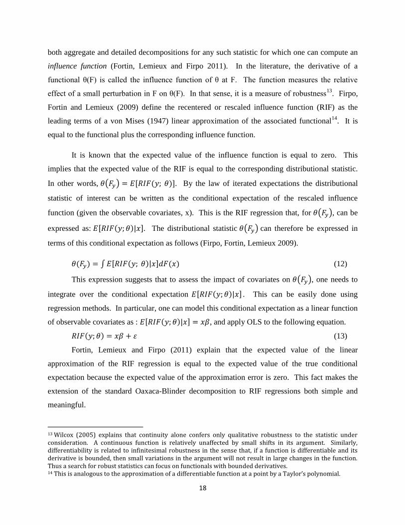
It is known that the expected value of the influence function is equal to zero. This

implies that the expected value of the RIF is equal to the corresponding distributional statistic.

In other words, . By the law of iterated expectations the distributional

statistic of interest can be written as the conditional expectation of the rescaled influence

function (given the observable covariates, x). This is the RIF regression that, for , can be

expressed as: . The distributional statistic can therefore be expressed in

terms of this conditional expectation as follows (Firpo, Fortin, Lemieux 2009).

(12)

This expression suggests that to assess the impact of covariates on , one needs to

integrate over the conditional expectation . This can be easily done using

regression methods. In particular, one can model this conditional expectation as a linear function

of observable covariates as : , and apply OLS to the following equation.

(13)

Fortin, Lemieux and Firpo (2011) explain that the expected value of the linear

approximation of the RIF regression is equal to the expected value of the true conditional

expectation because the expected value of the approximation error is zero. This fact makes the

extension of the standard Oaxaca-Blinder decomposition to RIF regressions both simple and

meaningful.

13 Wilcox (2005) explains that continuity alone confers only qualitative robustness to the statistic under consideration. A continuous function is relatively unaffected by small shifts in its argument. Similarly, differentiability is related to infinitesimal robustness in the sense that, if a function is differentiable and its derivative is bounded, then small variations in the argument will not result in large changes in the function. Thus a search for robust statistics can focus on functionals with bounded derivatives. 14 This is analogous to the approximation of a differentiable function at a point by a Taylor’s polynomial.

19

Applying the standard Oaxaca-Blinder approach to equation (13) we find that the

endowment effect can be written as follows.

(14)

The corresponding structural effect is

(15)

This decomposition may involve a bias since the linear specification is only a local

approximation that may not hold in the case of large changes in covariates15

. The solution to this

problem, consistent with our discussion in subsection 2.2, is to combine reweighing with RIF

regression (see Fortin, Lemieux and Firpo 2011) for details.

3. Endowment and Price Effects along the Entire Outcome Distribution

The presentation of the basic framework in section 2 focuses on the decomposition

of aggregate statistics. As noted in the introduction, these statistics provide little

information about the heterogeneity of impacts underlying aggregate outcomes. This

section therefore applies the same framework to the identification and estimation of the

aggregate endowment and price effects along the whole distribution of outcomes. All the

methods reviewed in this section are purely statistical in the sense that they all rely on

models of the conditional distribution of outcomes given the covariates. We consider in

turn the decomposition of differences in density functions and across quantiles. The

decomposition across quantiles also allows the analyst to express changes in poverty in

terms of endowment and price effects. The decomposition of changes in density functions

relies on nonparametric methods. In the case of quantiles, we focus on parametric

methods. Along the way, we note circumstances under which the contribution of

unobservables in the structural effect can be distinguished from that of observables.

3.1 Differences in Density Functions

For decomposition purposes, one needs a model that links the outcome of interest

to household characteristics. To focus on differences in density functions, we maintain that

the outcome variable y has a joint distribution with characteristics, x. This distribution is

15

In particular, and may differ just because their estimation is based on different distributions of the covariates x, even if the outcome structure remains unchanged (Firpo, Fortin and Lemieux 2009).

20

characterized by the following joint density function: . The generalization of

the Oaxaca-Blinder decomposition considered here requires the marginal distribution of y

noted as: . This marginal density function can be obtained by integrating the

covariates x out of the joint density. Furthermore, the factorization principle allows one to

write the joint density as a product of the distribution of y conditional on x, , and the

joint distribution of characteristics, . These are the two factors underpinning the

decomposition. Any change in the marginal outcome distribution induced by a variation in

the distribution of observed characteristics (ceteris paribus) represents the endowment

effect, while any change in the distribution associated with a (ceteris paribus) variation in

the conditional distribution is interpreted as the price-behavioral effect (Bourguignon and

Ferreira 2005).

To see clearly what is involved16, we express the joint density function as a product

of the two underlying functions: . On the basis of this

factorization, we can write the marginal density of y in a way that facilitates the expression

and interpretation of the decomposition results, that is: . Thus the observed

change in the outcome distribution between the two periods can be stated as follows.

(16)

We can add to and subtract from the difference defined in (16) the following

counterfactual17: . This is the marginal density function that would obtain if the

conditional distribution were that of period 0, and the joint distribution of characteristics

16 This account draws on Essama-Nssah and Bassolé (2010) 17

To clarify our notation, we consider the simplest case where x represents a single characteristic. No loss of

generality is involved. The marginal distribution of y is equal to

, where mx stands for the

maximum value of x. Equivalently,

. The counterfactual used in equation

(17) is therefore defined as follows:

. This expression can be derived from the

marginal outcome distribution in the initial period,

, by replacing with .

As explained in footnote 11, for this operation to lead to a meaningful counterfactual, two invariance conditions

must be met. The conditional distributions must be invariant with respect to changes in the marginal

distribution of observables, . This would be the case if there are no general equilibrium effects. The

distribution of unobservables must be at least conditionally independent of that of observables. Ignorability

guarantees this.

21

that prevailing in period 1. This transformation leads us to the following generalized

decomposition of changes in the marginal density of y.

(17)

The configuration of the indices (subscripts and superscripts) for the marginal

distributions involved in (17) suggests an interpretation of the various components of the

decomposition. The first component on the right hand side is the endowment effect (based

on changes in the joint distribution of observed characteristics). The second component

measures the price-behavioral effect (linked to the change in the conditional distribution of

y which, in fact, also includes the effect of unobservables).

In their study of the role of institutional factors in accounting for changes in the

distribution of wages in the U.S., DiNardo, Fortin and Lemieux (1996) demonstrate how to

implement empirically the above decomposition using kernel density methods to estimate

the relevant density functions. The histogram is the oldest and most common density

estimator (Silverman 1986), and kernel methods may be viewed as ways of smoothing a

histogram. The basic idea is to estimate the density f(y) by the proportion of the sample that

is near y. One way of proceeding is to choose some interval or “band” and to count the

points in the band around each y and normalize the count by the sample size multiplied by

the bandwidth. The whole procedure can be viewed as sliding the band (or window) along

the range of y, calculating the fraction of the sample per unit within the band, and plotting

the result as an estimate of the density at the mid-point of the band (Deaton 1997)18.

The kernel estimate of the density function can be written as follows.

. (18)

18 Deaton (1997) further explains that the size of the bandwidth is inversely related to the sample size. The larger the sample size, the smaller the bandwidth. To obtain a consistent estimate of the density at each point, the bandwidth must become smaller at a rate that is slower than the rate at which the sample size is increasing. However, with only a few points, we need large bands to be able to get any points in each. By widening the bands, we run the risk of biasing the estimate by bringing into the count data that belong to other parts of the distribution. Hence, the increase in the sample size does two things. It allows the analyst to reduce the bandwidth and hence the bias in estimation (due to increased mass at the point of interest), it also ensures that the variance will shrink as the number of points within each band increases.

22

where h is the bandwidth representing the smoothing parameter, nt is the sample size for

period t, y is the focal point where the density is estimated, and K(∙) is the kernel function.

A kernel function is essentially a weighting function chosen in such a way that more weight

is given to points near y and less to those far away. In particular, it will assign a weight of

zero to points just outside and just inside the band. As a weighting function, the kernel

function should satisfy four basic properties: (i) positive, (ii) integrate to unity over the

band, (iii) symmetric around zero so that points below y get the same weight as those an

equal distance above, (iv) decreasing in the absolute value of its argument. The most

common kernel functions used in empirical work are the Gaussian and the Epanechnikov

kernel19.

The counterfactual density function that is the linchpin of the decomposition

presented in equation (17) can be written in a manner analogous to the distribution

functions underlying the decomposition presented in equation in (9)20. In other words,

. This density can be estimated by reweighing the kernel estimate for

period 0 using the same weighing function as the one underlying the counterfactual

distribution defined in equation (11). The resulting expression is:

(19)

Machado and Mata (2005) propose a semi-parametric approach to estimating the

density functions needed in the above decomposition. Their approach is based on a two-

step procedure that allows them to derive marginal density functions from the conditional

quantile process that fully characterizes the conditional distribution of y given the

covariates x. Specifically, these authors model the conditional distribution of y given x by a

linear conditional quantile function as follows.

(20)

19 Deaton (1997) argues that the choice of the bandwidth or the smoothing parameter is more important than that of the kernel function. Essentially, estimating densities by kernel methods is an exercise in smoothing the sample observations into an estimated density. The bandwidth controls the amount of smoothing achieved. Over-smoothed estimates are biased, while under-smoothed ones are too variable. 20

The equivalent expression for the decomposition is: .

23

The second step in the approach entails estimating the marginal density function of

y that is consistent with the conditional quantile process defined by (20). This is achieved

by running the following algorithm: (i) Draw a random sample of size m from a uniform

distribution on [0, 1] to get τj for j=1, 2, , m; (ii) For each τj, use available data to estimate

the quantile regression model and get m estimates of coefficients ; (iii)

Given that xt is a (nt x k) matrix of data on covariates, draw a random sample of size m from

the rows of xt and denote each such sample by ; (iv) The corresponding values of the

outcome variable are given by:

. The validity of this procedure

stems from the probability integral transformation theorem which states that, if u is a

random variable uniformly distributed over [0, 1], then is distributed like F.

Here τj is assumed to be a realization of . Given model (20), the corresponding

conditional quantile regression model can be written as (Fortin, Lemieux and Firpo 2011):

(21)

A modified version of the above algorithm leads to the critical counterfactual upon

which the decomposition is based. Recall that the counterfactual of interest is the density

function of the outcome in period 1 assuming that the characteristics of that period had

been rewarded according to the system prevailing in period 0. This counterfactual can be

estimated by applying the above algorithm to the data for period 0, except that at stage (iii)

covariates must be drawn from data for period 1. On the basis of equation (21), the

conditional regression model associated with this counterfactual is the following.

(22)

As noted by Fortin, Lemieux and Firpo (2011), this approach is computationally

demanding. They suggest a simplification based on the estimation of a large number of

quantile regressions (say 99) instead of using the random process. The conditional

quantile function can then be inverted to obtain the conditional cumulative distribution

which must be averaged over the empirical distribution of the covariate to yield

unconditional distribution function. In fact, Machado and Mata (2005) acknowledge that

this is a viable alternative to their method.

24

3.2 Differences across Quantiles

One can also work with quantiles instead of density functions (or equivalently,

distribution functions) to decompose changes along the entire outcome distribution. Since

the decomposition must be based on marginal distributions, one needs to work with

marginal quantiles, not conditional ones. There is a variety of ways to go about it. Recall

that the general decomposition presented in section 2 about a distributional statistic θ(Fy)

applies to any statistic including quantiles. In that case, the counterfactual distribution is

derived from equation (11). Alternatively, marginal quantiles can be derived from

equations (20) and (21) based on the Machado and Mata (2005) procedure or by numerical

integration as proposed by (Melly 2005).

To link conditional quantiles to marginal quantiles, Angrist and Pischke (2009) start

from the observation that the proportion of the population below qτ conditional on x is

equal to the proportion of conditional quantiles that are below qτ. Let I(∙) be the indicator

function that takes a value of 1 if its argument is true and 0 otherwise. Again, let

stand for the conditional cumulative distribution function (CDF) of y given x. Thus the

proportion of the population for which the outcome y is less than qτ is equal to:

, where the term on the right hand side is equal to the

proportion of conditional quantiles that are below qτ. On the basis of equation (20), we can

rewrite this proportion as :

. The marginal distribution of y,

from which one derives marginal quantiles, is obtained by integrating the conditional

distribution over the whole range of the distribution of the covariates (Melly 2005). The

resulting expression is:

. The sample analog of this

expression based on an estimation of quantile regressions at every percentile for a sample

of size n is given by the following expression (Angrist and Pischke 2009).

(23)

25

The marginal quantile corresponding to the above estimator of the marginal distribution of

the response variable is obtained by inverting (23). We note these marginal quantiles

as: .

The generalized Oaxaca-Blinder decomposition described by equation (9) can

equivalently be stated in terms of these marginal quantiles. The observed change in the

marginal distribution of the response variable is now written as:

. To distinguish the endowment effect from the price effect, we subtract from

and add to this expression the following counterfactual outcome: . This

counterfactual involves the characteristics of period 1 evaluated with the prices

(coefficients) of period 0. The corresponding decomposition analogous to expression (9) is

the following.

(24)

Consistent with equation (9), the first term on the right hand side of (24) is the endowment

effect at the τth quantile while the second term measures the price effect at the same

location.

As noted in section 2, one can use RIF regression to perform detailed decomposition

of differences across quantiles. Firpo, Fortin and Lemieux (2009) show that the rescaled

influence function of the τth

quantile of the distribution of y is the following21

:

(25)

Where I(∙) is an indicator function for whether the outcome variable y is less than or equal to the

τth

quantile and fy(qτ) is the density function of y evaluated at the τth

quantile. Essama-Nssah et

21 Essama-Nssah and Lambert (2011) show how to derive the influence function of a functional from the associated directional derivative. They present a collection of influence functions for social evaluation functions commonly used in assessing the distributional and poverty impact of public policy. Their catalog includes, among others, influence functions and recentered influence functions for the mean, the τth quantile, the Gini coefficient, the Atkinson index of inequality, the class of additively separable poverty measures defined in equation (27) below, the growth incidence curve ordinate, the Lorenz curve and generalized Lorenz curve ordinates, the TIP curve ordinate and some measures of pro-poorness associated with the Foster, Greer and Thorbecke (1984) family of poverty measures.

26

al. (2010) apply this methodology to account for heterogeneity in the incidence of economic

growth in Cameroon.

At this stage we pause, to consider the implications of this decomposition for

poverty comparison over time. One can use equation (24) repeatedly to decompose, the

first 99 quantiles (percentiles) of the outcome distribution of interest. This means that we

can decompose the growth incidence curve22 (GIC) in a component due to the endowment

effect and another due to the price effect. Formally, we express this decomposition as

follows.

(26)

where the first component on the right hand side of (26) is the endowment effect for the

GIC and the second term is the corresponding structural effect.

For the class of additively separable poverty measures, a change in poverty over

time can be written as a weighted sum of points on the growth incidence curve (Essama-

Nssah and Lambert 2009, Ferreira 2010). Therefore, change in poverty over time inherits

the decomposability of the growth incidence curve. To see what is involved here, note that

the class of additively separable poverty measures is defined by the following expression:

(27)

where F stands for the distribution of a continuous outcome variable y and z is the poverty

line. This expression makes it clear that the poverty measure P(∙) can be viewed as a

functional of F. In other words, a poverty measure reveals the level of aggregate poverty

associated with a distribution and a poverty line. The term is a convex and

decreasing function measuring deprivation for an individual with a level of economic

welfare equal to y. This function is equal to zero when the welfare indicator is greater or

equal to the poverty line. For members of the additively separable class defined by (27), a

change in poverty associated with the growth pattern depicted by the incidence curve

is given by the following expression:

22

Ravallion and Chen (2003) define the growth incidence curve as the growth rate of an indicator of welfare

(income or consumption) y at the pth

percentile point of its distribution. The outcome at that point can be noted a

y(p).

27

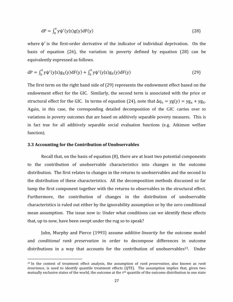
0 (28)

where is the first-order derivative of the indicator of individual deprivation. On the

basis of equation (26), the variation in poverty defined by equation (28) can be

equivalently expressed as follows.

0

0 (29)

The first term on the right hand side of (29) represents the endowment effect based on the

endowment effect for the GIC. Similarly, the second term is associated with the price or

structural effect for the GIC. In terms of equation (24), note that .

Again, in this case, the corresponding detailed decomposition of the GIC carries over to

variations in poverty outcomes that are based on additively separable poverty measures. This is

in fact true for all additively separable social evaluation functions (e.g. Atkinson welfare

function).

3.3 Accounting for the Contribution of Unobservables

Recall that, on the basis of equation (8), there are at least two potential components

to the contribution of unobservable characteristics into changes in the outcome

distribution. The first relates to changes in the returns to unobservables and the second to

the distribution of these characteristics. All the decomposition methods discussed so far

lump the first component together with the returns to observables in the structural effect.

Furthermore, the contribution of changes in the distribution of unobservable

characteristics is ruled out either by the ignorability assumption or by the zero conditional

mean assumption. The issue now is: Under what conditions can we identify these effects

that, up to now, have been swept under the rug so to speak?

Juhn, Murphy and Pierce (1993) assume additive linearity for the outcome model

and conditional rank preservation in order to decompose differences in outcome

distributions in a way that accounts for the contribution of unobservables23. Under

23 In the context of treatment effect analysis, the assumption of rank preservation, also known as rank invariance, is used to identify quantile treatment effects (QTE). The assumption implies that, given two mutually exclusive states of the world, the outcome at the τth quantile of the outcome distribution in one state

28

additive linearity, the function defining the outcome variable is separable in x and ε. We

can therefore write the outcome model as follows:

(30)

Where , some function of unobservable characteristics.

The assumption of conditional rank preservation means that a given individual has

the same rank in the distribution of as in the distribution of , conditional on her

observable characteristics. To see this formally, let stand for the distribution of

conditional on . Also, let be the rank of individual i with

observed characteristics xi in the conditional distribution of given x, and

her rank in the conditional distribution of given x. Conditional rank

preservation says that . Fortin, Lemieux and Firpo (2011) explain that one

can secure conditional rank invariance by assuming ignorability and that the functions

are strictly increasing in ε. In other words, these functions are monotonic24.

As expected, separability allows the analyst to construct counterfactuals separately

for observables and unobservables. To see what is involved, consider the case of a

particular individual, i, with outcome in period 1. Let represent what

the residual part of the outcome would have been, had the unobservable characteristics of

this individual been treated as in the initial period, ceteris paribus. The corresponding

counterfactual for the full outcome is:

. Comparing this counterfactual

with the observed outcome reveals the contribution of changes in the returns to

has its counterpart at the same quantile of the outcome distribution in the alternative state. Bitler et al. (2006) explain that when this assumption fails, the QTE approach identifies and estimates the difference between the quantiles and not the quantiles of the difference in outcome distributions. Rank preservation is akin to anonymity or symmetry used to base growth incidence analysis on cross-section data instead of panel data. Anonymity implies that when comparing two outcome distributions, the identity of the individual experiencing a particular outcome is irrelevant (Carneiro, Hansen and Heckman 2002). Thus, a permutation of outcomes between any two individuals in any of the two distributions being compared has no effect on the comparison. One might as well then compare such distributions across quantiles. 24 Recall that ignorability means that the conditional distribution of ε is the same across groups (or periods). Thus individuals with the same set of observable characteristics find themselves at the same rank in both (conditional) distributions. It is well known that a monotonic transformation preserves order. In fact, Rapoport (1999) defines a monotone transformation as “a formula that changes the numbers of one set to the numbers of another set while preserving their relative positions on the axis of real numbers.” Since is obtained from ε through a monotonic transformation , rank preservation must therefore follow.

29

unobservable characteristics of individual i in the overall change in her outcome. We

denote this by:

. Next, we replace with in the

expression for . This operation yields the following counterfactual:

.

Let

. This term is equivalent to

and clearly shows the

contribution of changes in the returns to observable characteristics. Thus, separability

along with ignorability and monotonicity make it possible to split the structural effect into

a component due to changes in the returns to observables and the other linked solely to

changes in returns to unobservables. In other words, the total structural effect25 is equal

to:

. The observable composition effect

can be identified residually

from the following expression:

where

. The assumption

of conditional independence implies however that

. Recall that this assumption

implies that the conditional distribution of unobservables does not vary across groups

(periods). Therefore, under the prevailing identifying assumptions, the difference between

the overall outcome difference and the structural effect identifies the observable

composition effect.

The question now is, how does one identify ? This is where rank preservation

comes in. This assumption leads to the following imputation rule.

(31)

This imputation rule says that, for individual i in the end period, the counterfactual for the

residual outcome is equal to the residual outcome associated with the individual located at

the same rank in the conditional distribution of residual outcomes in the base period. In

practice, one would estimate β0 and β1 using OLS. Bourguignon and Ferreira (2005)

25 Note that the structural effect can also be expressed as

. In the notation associated with

equation (8), linearity and rank preservation imply that corresponds to the counterfactual outcome

obtained by replacing the outcome structure φ1(∙) with φ0(∙). In other words, is the same as . This

suggests that the Juhn-Murphy-Pierce (1993) decomposition can be performed in two steps as follows. Start

with the overall difference

. Then add to and subtract from this difference the

counterfactual outcome . This yields a twofold decomposition of the overall difference into the

composition and structural effects. Finally add to and subtract from the structural effect the counterfactual outcome

. This step leads to the final threefold decomposition. Ignorability guarantees that the composition effect is due solely to changes in the distribution of observables.

30

explain that empirical implementation of a rank-preserving transformation is complicated

by the fact that both samples do not necessarily have the same number of observations.

However, if one is willing to assume that both distributions are the same up to some

proportional transformation, then the rank-preserving transformation can be

approximated by multiplying residuals in the base period by the ratio of the standard

deviation in the end period to the one in the initial period.

Fortin, Lemieux and (2011) point out that assuming constant returns to

unobservable and homoskedasticity allows one to write the unobserved component of the

outcome as . Homoskedasticity implies that the conditional variance of ε is

constant (and can be normalized to 1). Equation (30) can therefore be written as follows.

(32)

As it turns out, this is the version of the model used by Juhn, Murphy and Pierce (1991) in

their study of the evolution of the wage differential between Blacks and Whites in the U.S.A.

In that context, the standard deviation of the residuals in the wage equation stands for both

within-group inequality in the wage distribution and the price of unobserved skills (Yun

2009).

The outcome model specified in equation (32) has also been used to study gender

pay gap. In that context, t=1 is taken to represent males while t=0 stands for females, and

the wage regime for males is considered the non-discriminatory one. The counterfactual

used in the decomposition is the outcome female workers would have experienced if they

had been paid like their male counterparts. Care must be taken when applying this version

of the model to decompose differences in mean outcome using OLS since the OLS residuals

sum up to zero. To see this, consider the following expression of standard Oaxaca-Blinder

decomposition that explicitly shows the residuals.

(33)

The terms associated with the unobservables in the right hand side of equation (33) will

disappears if the decomposition is based on OLS applied to each equation separately.

31

To get around this issue, Juhn, Murphy and Pierce (1991) assume that the returns to

observable characteristics are the same for both groups and apply OLS to only one group,

and construct an auxiliary equation for the other group. In the context of gender wage gap

studies, OLS is applied to the equation for males only. The equation for female workers is

constructed as follows: . The implied decomposition is:

(34)

where

. The above expression is computed on the basis of the sample analogs of the

parameters of interest. The first term in the twofold decomposition presented in (34)

represents the predicted gap while the second stands for the residual gap. As Yun (2009)

points out, the residual gap is equal to the structural effect in the standard Oaxaca-Blinder

decomposition. Yet, this structural effect represents returns to observable characteristics.

It is therefore hard to see how the Juhn, Murphy and Pierce (1991) procedure helps

identify the contribution of unobservables. Yun (2009) proposes instead the

decomposition defined by equation (33), under the assumption that the expected value of

unobservable terms is not equal to zero. However, that author does not provide an

implementation procedure corresponding to this situation.

4. Behavioral Responses to Changes in the Socioeconomic Environment

A key limitation of both the basic Oaxaca-Blinder decomposition and its generalization

along the lines discussed in sections 2 and 3 is that they do not account for changes in the

behavior of agents in response to changes in their socioeconomic environment which may be due

to shocks or policy reform. Given the maintained hypothesis that the living standard of an

individual in a given society depends crucially on what he decides to do with his assets (innate

and external) subject to the opportunities offered by society, this section focuses on ways of

modeling agents’ behavior to account for their reaction to changes in their socioeconomic

environment. Standard economic theory explains behavior in terms of the principles of

optimization and market interaction. Modeling behavior entails the specification of the

following elements (Varian 1984): (i) actions that a socioeconomic agent can undertake,

(ii) the constraints she faces, and (iii) the objective function used to evaluate feasible

actions. The assumption that the agent seeks to maximize the objective function subject to

32

constraints implies that outcome variables used to represent the consequences of behavior

can be expressed as functions of parameters of the socioeconomic environment, embedded

in the constraints facing the agent. We consider two basic modeling frameworks, namely

the consumption-leisure choice paradigm and the Roy (1951) model of choice and

consequences. While both frameworks stem from the optimization principle, the

consumption-leisure choice model is a straight forward interpretation of standard

consumer choice theory in cases where the choice set is continuous. The Roy model

applies to discrete choice problems.

4.1. The Consumption-Leisure Choice Paradigm

We first describe the structure of this framework and then explain how counterfactual

decomposition can be performed on the basis of an empirical model. Known limitations of the

framework will also be noted along the way.

Structure

Standard neoclassical labor supply models are framed within the logic of individual

choice between consumption goods, c, and leisure, ℓ. This framework helps one establish the

determinants of labor supply and the conditions for participation in the labor market. Given a

wage rate, w, and non-wage income y, the consumer is assumed to maximize a utility function of

consumption and leisure subject to the full income constraint based on time endowment. Let ℓmax

be the time endowment representing the maximum amount of leisure the agent can enjoy. The

length of time worked is equal to: . Formally, the agent’s problem can be stated

as: . Equivalently, we have the following representation in terms of

the indirect utility function.

(35)

where p stands for the price of consumption normalized to unity in the budget constraint and m0

defines full income. This formulation of the problem suggests that the wage rate is viewed both

as the price and the opportunity cost of leisure. Two basic income sources determine the choice

set along with the price of consumption and the wage rate. These are activities within and

without the labor market.

The solution to the above optimization problem will lead to an observed supply of labor

that is greater or equal to zero indicating respectively participation and nonparticipation in the

labor market. Whether or not the agent decides to participate in the labor market depends on a

33

comparison of the wage rate with the trade-off she is willing to make between consumption and

leisure as characterized by her utility function (Cahuc and Zylberberg 2004). Within this

standard model, it is assumed that both consumption and leisure are normal goods and that the

agent is willing to sacrifice less and less consumption for each extra unit of leisure. The rate at

which the agent is willing to trade leisure for consumption is indicated by the marginal rate of

substitution defined by:

. The agent is willing to supply labor as long as the

marginal rate of substitution is less than the market wage rate. At the optimum, the marginal rate

of substitution is equal to the wage rate26

. Thus the wage rate at which the agent finds it optimal

to supply zero hours of work is known as the shadow or the reservation wage (Deaton and

Muellbaouer 1980, Cahuc and Zylberberg 2004). At this point, the agent has no labor income, so

that the maximum value of consumption is equal to y0. Since the time endowment is fixed, the

reservation wage is a function mainly of non-labor income. When leisure is a normal good, any

policy that leads to an increase in non-wage income will increase the reservation wage and will

thus have a disincentive effect on the participation decision. The reservation wage thus

determines the conditions of participation in the labor market.

As an outcome of the optimization process described by (35), the Marshallian demand for

leisure and the corresponding Marshallian supply of labor depend on two parameters, the wage

rate, w, and full income m0 which also depends on the wage rate (the opportunity cost of leisure).

It is important to note how a change in the wage (possibly induced by policy or other factors in

the socioeconomic environment) might affect the supply of labor. To be specific, consider an

increase in the wage rate. This increase will affect the demand for leisure through conventional

substitution and income effects. Since leisure is assumed to be a normal good, these two effects

combine to reduce the demand for leisure hence to increase the supply of labor. In addition to

these effects, an increase in the wage rate increases the value of full or potential income. This

would induce an increase in leisure or a decrease in labor supply. Cahuc and Zylberberg (2004)

refer to the conventional income effect as the “indirect” income effect, and call “direct” income

effect the one linked to potential income. The overall effect of a change in the wage rate is

26 To see clearly what is involved, consider the case where MRSℓc<w. This implies that the marginal utility of leisure is less than the leisure value of the marginal utility of consumption. It is therefore desirable for the agent to increase consumption relative to leisure. Assuming decreasing marginal utility, increasing consumption will progressively bring down the marginal value of consumption until equilibrium is reached indicating the optimal combination of consumption and leisure.

34

therefore ambiguous. It depends on which group of effects dominates. In any case, the shape of

the labor supply curve is determined by the interaction among these effects.

Bourguignon and Ferreira (2003) expand the basic framework to include individual

characteristics and the net tax system. It is assumed that, an economic agent with characteristics

z chooses between consumption and leisure (or labor supply) so as to maximize utility subject to

a budget constraint that explicitly incorporate the net tax system27

. Formally, the problem is

stated as follows.

(36)

In this expression, nt(·) represents the tax-benefit schedule, a function of the agent’s

characteristics, his labor income (wh), his exogenous non-labor income (y), and possibly the

level of labor supply, h. The parameters defining the tax-benefit system such as tax rates or the

means-testing of benefits are represented by ξ. There are also parameters such as β and ε

characterizing preferences along with agent’s characteristics, z.

Individuals are members of families or households. One would expect that the family or

the household will have a considerable influence on decisions made by its members, including

labor supply decisions. It is therefore instructive to consider how the basic model discussed so

far has been adapted to account for the potential influence of the structure of the household to

which an individual belongs. A straightforward extension of the neoclassical model to

household-level supply of labor has taken the form of the so-called unitary model (Blundell and

MaCurdy 1999). A key characterization of this model is the assumption of “income pooling”

which implies that the level of household consumption is determined by the common pool of

resources available for various household members. The household can therefore be viewed as

single agent with its own utility that depends on total consumption and individual members’

consumption of leisure. Within this framework, individual labor supply functions depend on the

household full income, the price of consumption and the wage rates.

The analysis of household choices can also be framed within the logic of the collective

model. This approach insists on the principle that choices made by a household must reflect the

preferences of its members and is consistent with the assumption that individual decisions made

27 This constraint may also include the fixed cost of employment as a function of individual characteristics. This cost may include cost incurred for child-care while at work. Accounting for this dimension makes it possible to simulate the implications of policy designed to compensate individuals or households for child care (Creedy and Duncan 2002).

35

within the household are Pareto efficient so that there are no opportunities for mutually

advantageous allocation (Cahuc and Zylberberg 2004). In the context of this framework,

decisions made by individual i are an outcome of the following mathematical program.

(37)

where si is interpreted as a “sharing rule” determining the share that each household member gets

out of total non-wage income of the household. This variable is a function of the wage rate faced

by the individual and her contribution in non-wage income. Interestingly, this formulation offers

the possibility of inferring the consumption of individual household members which is not

necessarily observable. Given the interdependence among choices of different members of the

household, this approach makes it easier to understand why certain members of the household

may choose to specialize in household production while others may supply their labor to relevant

markets. This interdependence also suggests that variations in individual’s income affect not

only his labor supply decisions, but those of the other members of the household as well.

One key feature limiting the applicability of the basic model of consumption and leisure

choice to the study of behavioral responses to shocks and policies is the assumption of a linear

budget constraint. More generally, Deaton and Muellbauer (1980) argue that the simple

neoclassical labor supply model has limited usefulness for policy analysis because it does not

account for issues related to aggregation, participation decisions, constraints on hours worked

and unemployment. With respect to the number of hours worked, Salanié (2003) notes that

individual choice may be constrained by existing labor market regulations. Furthermore, part

time work may not be an outcome of free choice, but rather a reflection of the difficulty in

finding full time employment. It is therefore important to consider the participation decision.

Counterfactual Decomposition

In principle, the solution of the program specified in (36) for individual i (or a household

depending on the unit of analysis) leads to a simultaneous equation system describing the

demand for consumption and leisure. The demand for leisure can be translated into a labor

supply function. Given relevant data, the model composed of the consumption and labor supply

can be estimated simultaneously first using baseline data, then using end period data.

Counterfactual simulations can then be conducted by switching parameters and variables

between the two estimated models in order to identify the effect of the factor that was changed

36

while holding all the others constant. This, again, is an application of the ceteris paribus

identification strategy.

Bourguignon and Ferreira (2003), in the context of ex ante evaluation of policy reforms,

propose a recursive approach that can be adapted to the types of decompositions considered here.

These authors note that the program stated in equation (36) leads, for individual i, to a nonlinear

labor supply function of the form:

. (38)

where the εi are the idiosyncratic preference terms analogous to the random disturbance terms in

standard regression analysis. Given a reliable cross-section data set, estimation procedures seek

to minimize the role of these idiosyncratic terms in explaining cross-sectional variations in labor

supply. This will produce a set of estimates for preference parameters and for the

idiosyncratic preference terms. The fact that the preference parameters have no subscript here

implies that they are assumed common to all agents. The estimated version of equation (38) can

be written as follows.

. (39)

Given a baseline estimate of the labor supply function, it is possible to simulate, for

instance, the implications of alternative tax-benefit system for labor supply and consumption by

changing relevant components of ξ, and comparing the new results to the base line.

To fix ideas, let be the labor supply observed for

individual i at time t=0, 1. Consider an experiment where the tax system prevailing in the end

period is imposed on agents in the baseline period, ceteris paribus. Let

be the corresponding labor supply. The change in labor supply

due to this change is equal to the following.

(40)

Under the simplifying assumption that consumption is equal to disposable income28

, the budget

constraint implies that the corresponding change in consumption is equal to:

(41)

where . These changes in the

indicator of economic welfare can then be used to compute the changes in poverty (or any other

28 No generality is lost here since one can always compute consumption as a fraction of disposable income.

37

social evaluation function) corresponding to the underlying ceteris paribus variation in the tax-

benefit system. While we used the tax benefit system to illustrate the principle, it is obvious that

the same principle applies to any of the arguments of the labor supply function, be it an

observable variable or an estimate of a parameter or term associated with preferences. The case

of idiosyncratic terms deserves special attention and we will come back to it in the next

subsection. Also, the discussion assumes that the individual is the unit of analysis. However, the

general principle carries over to the unitary model of household behavior.

There are serious difficulties associated with the estimation of labor supply models based

on this classical approach. These difficulties stem mainly from the assumed continuity of the

decision variable, hours of work, coupled with a lack of restrictions on this variable. Salanié

(2003) explains, in a simple framework, a structural estimation procedure applicable to this basic

model. The optimization process underlying the labor supply function has two possible

outcomes. The agent will supply zero hours if the reservation wage is greater than the market

wage, otherwise he will supply labor up to the point where the marginal rate of substitution

between consumption and leisure is equal to the wage rate. This equality defines a latent labor

supply function of the net wage rate, disposable non-labor income and an error term. Since

wages are observed only for people who work, a Tobit model of labor supply is estimated jointly

with a wage equation that includes individual characteristics (observable and idiosyncratic).

When a full tax-benefit system is included in the budget constraint, the marginal tax rate

is increasing and the budget constraint is convex, one can define a virtual wage rate on the basis

of the marginal tax rate and a virtual income based on this virtual wage in order to derived the

labor supply from an optimization problem that maximizes utility subject to the virtual budget

constraint. The fact that the virtual wage and income are endogenous means that we should

consider instrumental variable or maximum likelihood estimation methods. When the tax-

benefit system leads to non-convex budget constraints, one can no longer rely on first-order

conditions to find the optimum. The common approach is to consider discrete levels of labor

supply such as h=0, 10, 20, 30, 40 (hours per week) and compare utility values over the choice

set to find the maximum. Creedy and Duncan (2002) review a series of estimation procedures

that have been used in the empirical literature to deal with these difficulties. They conclude that

the structural discrete choice approach offers a more promising method. We briefly outline that

approach next, within the logic of the Roy (1951) model of choice and consequences.

38

4.2. The Roy Model of Choice and Consequences

This section reviews the structure of the basic Roy model along with its interpretation in

the context of modeling the determinants of the living standard as represented by household

consumption expenditure. It also discusses key considerations in simulating counterfactual

distributions underlying any decomposition exercise.

Structure and interpretations

Heckman and Honoré (1990) explain that the original Roy (1951) model was designed

for the study of occupational choice and its implications for the distribution of earnings in an

economy where agents are endowed with different sets of occupation-specific skills. In that

economy, income-maximizing agents can freely choose to work only in one of two activities,

fishing and hunting, on the basis of their productivity in each. Thus, an agent with a given skill

endowment will choose to work in the sector where her potential income is higher. There are no

investment opportunities for the augmentation of sector-specific skills nor are there costs

associated with changing sectors. These authors also show that self-selection implies a lower

level of inequality in earnings compared to a benchmark case where workers are randomly

assigned to jobs. The fact that occupational choice has significant implications for the

distribution of earnings makes the Roy model a relevant framework for the analysis of behavioral

responses by agents to changes in their socioeconomic environment.

Heckman and Sedlacek (1985) discuss an extension of the basic framework by including

nonmarket activity as an option in the choice set facing socioeconomic agents who are now

assumed to maximize utility instead of income. The utility of participating in each of the sectors

depends on both sector-specific attributes such as the wage rate or employment risk and job

status, and individual characteristics. The fact that we observe only sectoral choices and not the

underlying utility function means that it is possible to identify only parameters associated with

differences in utility across sectors. These authors also consider the contribution of self-selection

to income inequality and find that, in this general model, self-selection can increase both

between and within sector inequality compared to a random allocation of workers to sectors.

At the most fundamental level, the Roy model is characterized by two components,

namely, a selection mechanism and the associated potential outcomes. These outcomes are

possible consequences of the choice made through the selection mechanism. The extended

39

version of the Roy model is consistent with discrete choice models to the extent that utility

maximizing agents face a discrete choice set. Train (2009) characterizes a discrete choice model

in terms of two fundamental elements: the choice set and the decision process (or the decision

rule). The choice set is the collection of alternatives from which the decision maker chooses one.

This set must be exhaustive in the sense that it must include all possible alternatives, the latter

being mutually exclusive from the perspective of the decision maker. Finally, the number of

alternatives must be finite. In the case of discrete models of labor supply, for instance, the choice

set can be represented by a few options such as not working, working part-time and working full

time.

Just as in the case of the consumption-leisure paradigm, the decision process assumes

utility-maximizing behavior. It is therefore assumed that the decision maker chooses the

alternative that provides the greatest net benefit or utility. Let be the utility

agent h gets from alternative j. The decision rule implies that alternative k is chosen by the agent

if and only if . This decision making process is usually framed within the logic

of the random utility model where utility has two parts. The first, known as the representative

utility, is a function of some observable characteristics of the decision maker and of the

alternatives (Train 2009). The second component is a set of non-observable random factors.

Formally, the utility function is written as; where is the representative utility

and represents the unobserved portion of utility that is treated as random. Now, the statement

that alternative k is chosen if and only if can be equivalently expressed as: k is

chosen if and only if . Because of the uncertainty implied by

the random part of the utility function, one can only make probabilistic statements about the

decision maker’s choice. The probability that option k is chosen by agent h is defined by the

following expression29

:

(42)

29 The expression of this probability can be made more precise by considering an indicator function for the decision rule. The indicator is equal to 1 when option k is chosen and 0 otherwise. The probability that the agent chooses option k is then equal to the expected value of this indicator function over all possible values of the unobserved factors. In other words, . This is in fact a

multidimensional integral over the joint density of the random vector the elements of which represent unobserved factors associated with each alternative. This probability can be interpreted as the proportion of people within the population who face the same observable utility as h for each alternative and choose k (Train 2009).

40

The type of discrete choice model derived from the above probability statement is

determined by the assumptions made about the distribution of the unobserved portion of the

utility function. For instance, the common logit model assumes that the random factors are

independently and identically distributed (iid) extreme value variables for all options. In other

words, each choice is independent from the others30

.

Coulombe and McKay (1996) provide an interesting interpretation of the Roy model that

is consistent with our maintained hypothesis that the living standard of an individual is a pay-off

from her participation in the life of society. Using the household as the unit of analysis, these

authors argue that the living standard of a household depends fundamentally on the

socioeconomic group to which it belongs (or their economic activity status). To frame this view

within the logic of the Roy model, the authors further argue that one needs to explain the

selection mechanism leading to the observed socioeconomic group, and conditional on that

choice, the determinants of the living standard in that group. This logic leads to a two-equation

model, one representing the selection mechanism and the second modeling the living standard

conditional on the choice of a particular socioeconomic group.

Modeling the selection mechanism boils down to modeling the probability defined in

equation (42). Consistent with the random utility framework underlying this expression, and

assuming that the random elements are generated independently by an extreme value

distribution, the multinomial logit model can be used to explain the probability of choosing an

option. Formally, we express that probability as:

(43)

where zhj is the set of relevant explanatory variables and m is the total number of socioeconomic

groups. The probability defined in (43) is essentially the propensity score.

The specification of the explanatory variables requires a good understanding of the

determinants of the choice of a socioeconomic group. Autor (2009) explains that there are three

30 The generalized extreme value model (GEV) allows correlation among unobserved factors. The standard multinomial logit assumes that the random factors are iid with a double exponential distribution. The probit model assumes that the random factors are jointly distributed normal variables. Train (2009) points out that the identification of discrete choice models relies heavily on the fact that only differences in utility matter and the scale of utility is irrelevant. Hence, only parameters that capture differences across alternatives are identifiable and therefore estimable. This also implies that characteristics of the decision maker that do not vary across alternatives will have no effect unless they are specified in a way that induces differences in utility over alternatives. Glick and Sahn (2006) handle this problem by indexing the coefficients of sociodemographic variables in the representative utility function.

41

technological factors that affect this choice in the context of the general Roy model, namely: (i)

the distribution of skills and abilities, (ii) the correlations among these skills in the population

and (iii) the technologies for applying these skills. Coulombe and McKay (1996) make a similar

point in a case study of Mauritania. They define socioeconomic groups in terms of the income-

generating opportunities available to households and their members. In particular, they consider

four mutually exclusive and exhaustive groups of households: (i) households working

predominantly as employees (whether in the public or private sector), (ii) those engaged mostly

in self-employment in agriculture, (iii) those engaged mainly in non-farm self-employment, and

(iv) those not in the labor force. In essence, socioeconomic groups are determined on the basis

of the main economic activity of the household or the main source of income.

As to the determinants of the choice of socioeconomic groups, these authors argue that

the choice depend on variables (such as education, wage or profit rates) that affect relative

returns from economic activities as well as on consumption preferences. In particular, they make

the point that the extent to which household members choose self-employment over wage

employment or to stay out of the labor market depends on the interaction between total

household labor supply within and outside the household (a consumption decision) and it total

labor demand ( a production decision) for both household members and hired labor. In other

words, the socioeconomic classification of the household reflects both consumption parameters

such as the demographic composition of the household and the characteristics of the head of

household, and production parameters relevant to self-employment such as fixed inputs and

variable costs.

Equation (43) models the selection mechanism. We need an outcome equation to

complete the model within the logic of the Roy framework. Following Coulombe and McKay

(1996), we let yhk stand for the log of per capita expenditure for household h in socioeconomic

group k, and ηhk a random disturbance. The outcome equation associated with equation (43) can

be written by analogy to the standard Mincer equation (in labor economics) as follows.

(44)

Equations (43) and (44) constitute a system designed to explain living standard at the household

level. In their case study, Coulombe and McKay (1996) distinguish two categories of

determinants, demographic factors that are relevant to all households regardless of the group they

belong to. These demographic variables include household size, household composition, and

42

characteristics of the economic head of the household (e.g. education level, marital status, gender

and ethnicity). Group specific factors include those affecting the level of total household

income. For those engaged in wage employment, such factors would include level of education,

sector of employment and numbers of hours worked in a year to account for seasonal work.

Given that such variables are difficult to measure at the household level (the unit of analysis),

one could define and measure these variables only for the economic head of household or adopt

some form of aggregation over household members. Naturally, this would entail some loss of

the heterogeneity found at the individual level. In the case of agricultural self-employment,

specific factors include such things as land size and quality, tenure status, use of fertilizer,

insecticides, hired labor, access to extension services and commercialization. Similar

considerations apply to non-agricultural self-employment. For households outside the labor

market, possible sources of livelihood include assets holding, borrowing, public and private

transfers.

Another important consideration here is the classification of variables as exogenous or

endogenous. This classification hinges on the time horizon chosen. Coulombe and McKay

(1996) note, for instance, that in the long run the living standard can affect demographic

variables such as household size and composition. But in the short run it is reasonable to think

of the direction of influence as running from demographic variables to the living standard. In

their study, these authors adopt a short to medium time frame so that most of the variables listed

above are considered exogenous with respect to the model described by equation (43) and (44).

Bourguignon, Ferreira and Leite (2008) show how to expand this framework to model

changes in education and household demographics. In the extended framework, socioeconomic

group, per capita consumption, education and household composition are endogenous.

Variations in education and in household composition are modeled within the discrete choice

framework portrayed by equation (43). In that particular application, the demand for education

is modeled on the basis of six alternatives: 0 years of schooling; 1-4; 5-6; 7-8; 9-12; and 13 and

more. The highest level of education is the excluded category. The variables considered as

purely exogenous by these authors include: number of adults in the households, the region of

residence, age, race and gender. For household demographics, the options are: 0, 1, 2, 3, 4, 5 and

more children. The last category is omitted in the estimation. Note that education is an

explanatory variable in the demographic multilogit model. Leite, Sanchez and Laderchi (2009)

43

apply this extended framework to analyze the evolution of urban inequality in Ethiopia. They

too focus on the household as the unit of analysis and use per capita household expenditure as

the outcome variable.

Cogneau and Robilliard (2008) use the extended Roy model to study the implications of

targeted poverty reduction policies in Madagascar31

. While using the household as the unit of

analysis and considering consumption as the ultimate welfare indicator, these authors model first

the income-generating process at the level of individual members of the household, and then link

consumption to household income. The choice set facing individuals of working age (15 years

and older) includes three alternatives: family work, self-employment and wage work. Household

composition and location are exogenously given. For self-employment and wage work, the

potential earnings of an individual are equal to a task price times a given idiosyncratic amount of

efficient labor. Efficient labor is assumed to be a function of some observable characteristics

(such as age, experience and location) and unobservable skills. Family work is rewarded by a

reservation wage that is a function of individual and household characteristics32

. In the absence

of labor market segmentation, the simple selection rule of the basic Roy model would base sector

choice on a comparison of the reservation wage, and potential wages in the other two sectors. To

account for labor market segmentation, Cogneau and Robilliard (2008) define a segmentation

variable in terms of the relative cost of entry between self-employment and wage work, and

adjust the selection rule accordingly.

For the purpose of policy evaluation, these authors embed the occupational choice

model into a broader microeconomic module that includes the demand system for

consumption goods. To keep things simple, they assume that consumption or saving

decisions are separable from labor supply decisions. They also assume a fixed common

saving rate of 0.052 so that aggregate consumption is equal to the implied propensity to

consume times disposable income. The latter is the sum of farm profits, labor income,

earnings from self-employment, and nonlabor income such as capital income and transfers.

Total consumption is allocated to three composite goods (agricultural, informal and

31 These include (i) a direct subsidy on agricultural production prices, (ii) a workfare program and (iii) a uniform untargeted per capita transfer program. 32 For agricultural households, earnings are computed on the basis of a reduced farm profit function (based on Cobb-Douglas technology) that includes self-consumption and accounts for hired labor. For family members participating in farm work, the reservation wage (a measure of the value of family work) is assumed to depend on their contribution to farm profits.

44

formal) according to budget shares derived from available data. The three policies

considered have the potential of inducing large macroeconomic effects, because their cost

represents about 5 percent of gross domestic product (GDP). To account for this, the

authors link the micro module to a small three-sector (agriculture, informal and formal)

computable general equilibrium model. The integrated framework makes it possible to

consider the macroeconomic impact of the policy options along with their impact on

inequality and poverty. Adding a general equilibrium model removes a key limitation of

the decomposition methods discussed up to this point. These methods rely on either a

purely statistical or a microeconomic model of behavior that cannot account for general

equilibrium effects.

Simulating Counterfactual Distributions

The simulation of counterfactual distributions needed for the decomposition of

distributional changes proceeds in the same manner as in the case of the simultaneous model of

consumption and labor supply discussed above. We need to estimate some version of the Roy

system (composed of a selection equation and an outcome equation) for the initial and end

periods. Counterfactual distributions can then be simulated by switching parameters and

variables between these two estimated models one element at a time holding all the other factors

constant.

In general, parameters of sample selection models can be estimated with two-stage

methods or the maximum likelihood approach. We focus here on two-step procedures that

are also known as control function methods or generalized residual methods (Todd 2008). As

noted earlier, the selection mechanism is usually modeled within a random utility framework and

identifying assumptions are based on functional form restrictions or exclusion restrictions

(analogous to the instrumental variable approach). In particular, the control function approach

seeks to model conditional expectations of potential outcomes (given observable characteristics

and occupational or socioeconomic status) in a way that relates unobservable determinants of

outcomes to the observables, including the choice of a socioeconomic group. This is consistent

with the view that the underlying endogeneity problem is due to omitted variables. The control

functions represent the omitted variables. To fix ideas, consider a two-sector Roy model. Let d

45

be a dummy variable indicating the sector of activity. Thus we let d=1 for sector 1 (e.g. fishing)

and d=2 for sector two (hunting)33

with the corresponding potential outcomes y1 and y2.

Given observable characteristics x, z and socioeconomic status, d, the conditional

expectations of these potential outcomes can be written as:

(45)

Similarly,

(46)

Heckman and Navarro-Lozano (2004) explain that if one can model and

and find a way to cause these functions to vary independently of

and , then one can identify and up to constant terms. This is another

manifestation of the separability condition discussed earlier in section 3.

Consistent with the random utility framework underlying the selection model, we

assume that d=2 if some underlying index u is greater than zero.

Furthermore, if we assume that , then we have:

(47)

where is the propensity score. Similarly, assuming that

yields the following relation.

(48)

This approach is consistent with the view that the underlying endogeneity problem

is due to omitted variables. The control functions represent the omitted variables. The key

assumption in this framework that allows us to express each control function Kj(∙), j=1, 2

solely as a function of P(x, z) is the assumption that the observed individual characteristics

are independent of the unobservable determinants of selection and outcomes (a form of

ignorability) . This assumption, along with the rest of imposed restrictions, isolates a

33 We avoid using the traditional coding (0, 1) because we reserve it for the base and end periods respectively.

46

source of identifying variation in selection which helps to determine the parameters of

interest. The assumption is formally stated as follows:

(49)

Under these assumptions, the conditional expectations for the potential outcome are equal

to the following.

(50)

Similarly,

(51)

If we can use z to vary each control function holding x fixed, we can identify and

. We note that these control functions are designed to control for selection bias in the

estimation of the relevant parameters.

In the context of Heckman (1976, 1979) two-stage estimator, the control function is

known as the inverse Mills ratio. Hall (2002) points out the following drawbacks: (1) The

conventional standard error estimates are inconsistent, (2) the method does not impose

the constraint that the absolute value of the correlation coefficient be less than one, (3)

since the normality assumption is required for consistency, the estimator is no more robust

than the full maximum likelihood approach that also requires normality. Lee (1983)

proposes an alternative way of estimating the inverse Mills ratio, particularly when one

does not assume normality for the random error in the selection equation. This involves a

general transformation to normality as follows. Let qτ be the quantiles associated with the

predicted probabilities from the first stage of the process. The transformation computes

these quantiles by inverting the cumulative standard normal distribution applied to the

predicted probabilities. This is essentially an imputation procedure analogous to the one

discussed in section 3.

Once the model has been estimated, counterfactual decompositions are performed

following the same logic as in the case of the consumption-leisure model. Building on the

statistical approaches discussed in section 3, Bourguignon, Ferreira and Leite (2008) propose

47

the combination of parametric and nonparametric techniques in constructing the desired

counterfactuals. To see clearly what is involved, recall that the density function characterizing

the joint distribution of the outcomes and covariates can be written as a product of the two

underlying density functions, one characterizing the conditional distribution of outcomes

given the covariates and the other the joint distribution of covariates. Earlier, we

expressed this relation as: . As noted earlier, this

factorization suggests that counterfactual distributions can be obtained by combining the

conditional outcome distribution from one period (e.g. initial period) with the joint

distribution of covariates from the other period (e.g. the end period). An example of this

type of combinations would be the following:

(52)

A key distinction between the methods discussed in section 3 and those reviewed in

this section is that methods in section 3 are based on statistical models of the conditional

outcome distribution while the methods discussed here rely on economic modeling of this

conditional distribution. Thus, equations (43) and (44) characterizing the basic Roy model

must be seen as modeling the conditional outcome distribution . The method of

Bourguignon, Ferreira and Leite (2008) consists in using the parametric approach in

generating counterfactuals for the conditional outcome distribution and non-parametric

sample reweighing techniques to construct counterfactuals for the joint distribution of

exogenous covariates. They argue that the parametric approach for the conditional

distribution has the advantage of providing a clear economic interpretation of the

parameter estimates along with great flexibility in exchanging parameters from one period

to another (i.e. from one state of the world to another).

To see how this works in the context of the Roy framework, use the estimated model

to write the approximation to the conditional outcome distribution as follows:

(53)

Thus a change in the conditional outcome distribution due to a ceteris paribus change in the

parameters of the multinomial logit model of selection can be computed easily as follows.

(54)

48

When a counterfactual requires a normalization of exogenous covariates for both periods,

we can simply apply the DiNardo, Fortin and Lemieux (1996) approach described in

section 2. The handling of the residuals in this process requires some care. In the case of

the residuals associated with the outcome equations, for instance, one can resort to the

rank-preserving transformation described in section 3.

5. Concluding Remarks The design and implementation of effective strategies for poverty reduction require

a relevant and reliable analytical input. The bedrock of this analytical input is certainly a

rich and reliable data set (both qualitative and quantitative) to be used in poverty

measurement and analysis. In this context, there is a need for a sound understanding of the

fundamental factors that account for observed variations in poverty either across space or

over time. This paper reviews some of the basic decomposition methods that are

commonly used to identify sources of variation in poverty outcomes, both at the macro and

micro levels. The paper focuses on micro approaches because macro methods fail to

account for the heterogeneity of the factors that drive the observed changes in aggregate

poverty.

The decomposition of changes in poverty can be viewed as an exercise in social

impact evaluation understood as an assessment of changes in individual and social

outcomes attributable to socioeconomic shocks or policy implementation. All

decomposition methods reviewed in this paper obey the same logic of counterfactual

decomposition organized around the following terms: domain, outcome model, scope,

identification and estimation. The domain represents the type of distributional changes a

method seeks to decompose (e.g. changes in poverty over time or across space).

The outcome model links the outcome of interest to its determining factors. As

shown in the appendix, some macro-decomposition methods link variations in poverty to

changes in the mean and relative inequality characterizing the underlying distribution of

living standards. Others exploit the structure of additively decomposable measures to

decompose such variations into an intrasectoral effect and an effect due to population

shifts. Outcome models that underlie micro-decomposition methods are consistent with

the view that the living standard of an individual is a pay-off from her participation in the

49

life of society, and a function of endowments, behavior and the circumstances that determine

the returns to these endowments from any social transaction. These elements define the

potential scope of micro-decomposition methods. In general, the scope of a decomposition

method is the set of explanatory factors the method tries to uncover by decomposition.

The specification of an outcome model thus determines the potential scope of the

corresponding decomposition method.

The micro-decomposition methods reviewed in this paper fall into two basic

categories, namely statistical and structural. All seek to model the joint distribution of the

outcome variable and its determining factors. This joint distribution can be factorized into

a product of the conditional outcome distribution and the marginal distribution of

exogenous (independent) variables. Statistical methods rely uniquely on statistical

principles to model the conditional outcome distribution while structural methods rely on

both economics and statistics to model this object. In particular, the structural methods

considered here use utility maximization in a partial equilibrium setting to characterize

individual behavior and social interaction. Statistical methods therefore are purely

descriptive, while structural ones are considered predictive.

Identification concerns the assumptions needed to recover, in a meaningful way, the

factors of interest at the population level. These assumptions involve both the functional

form of the outcome model and the joint distribution of factors that determine the

outcome. While macro- and micro-decomposition methods differ in their scope, they share

the same fundamental identification strategy based on the notion of ceteris paribus

variation. The implementation of this idea entails the comparison of an observed outcome

distribution with a counterfactual obtained by changing one factor at a time while holding

all the other factors constant. A key counterfactual used in the identification of endowment

and price effects is the outcome distribution that would have prevailed in one state of the

world had individual characteristics been rewarded according to the system applicable in

the alternative state. The construction of this counterfactual relies critically on ignorability

and the absence of general equilibrium effects. When the outcome model is separable in

observables and unobservables, one can assume rank preservation to further split the price

effect into a component due to observables and another due to unobservable factors.

50

Estimation involves the computation of the relevant parameters on the basis of

sample data. There is a powerful analogy between the decomposition methods reviewed

here and treatment effect analysis. Both fields of inquiry rely on the same fundamental

identification strategy, and the structural effect is known to be equivalent to the treatment

effect on the treated. This analogy has led to the development of flexible estimation

methods for endowment and structural effects. Nonparametric estimation methods, such

as inverse probability weighing, allow the analyst to decompose distributional changes

without having to assume a functional form for the outcome model. The downside

however is the inability to further decompose the structural effect and to account for

behavior. Parametric methods are more suitable for these two tasks.

While the analogy between decomposition methods and treatment effect analysis

has helped with the development of estimation methods, it does not necessarily confer a

causal interpretation to decomposition results. As noted by Ferreira (2010), such an

interpretation requires the construction of counterfactual outcome distributions that are

fully consistent with a general equilibrium of the economy. One way of achieving this

consistency is to base decomposition on a full structural model of behavior and social

interaction. Such a model can be built by embedding a behavioral model, e.g. the Roy

(1951) model of choice and consequences, in a general equilibrium framework.

51

Appendix

Identification of Macro Factors

The macro-decomposition methods reviewed in this appendix are designed to

reveal aggregate factors that might explain variations in poverty over time or across

socioeconomic groups. As noted in the introduction, these macro methods rely on the same

identification strategy as the micro methods discussed in the main text. Each

decomposition method is characterized mainly by the nature of the factors it seeks to

reveal and the structure of the relationship it assumes between the focal object of

decomposition and its determining factors. The first group of methods we consider seek to

account for changes in poverty in terms of changes in the mean and in relative inequality of

the underlying outcome distribution. We refer to the component associated with the mean

as the size effect. The one associated with relative inequality will be called the

redistribution effect. The second group of methods we examine here exploit the structure

of additively decomposable poverty measures to characterize changes in poverty over time

in terms of intrasectoral effects and effects stemming from population shifts.

I. The Size and Redistribution Effects

There are two methods of decomposing variations in poverty outcome into the size

and redistribution effects. The first is a threefold decomposition that identifies a third

component as an indicator of the interaction between the two main effects (size and

redistribution). The second method, based on the Shapley value, involves no such term.

We review both methods along with ways of simulating relevant counterfactual outcomes.

A Threefold Decomposition

Datt and Ravallion (1992) observe that poverty measures may be fully characterized by

the poverty line, z, the mean of the distribution of economic welfare, μ, and relative

inequality as represented by the Lorenz curve L. When working with real income as an

indicator of economic welfare, the poverty line is considered fixed so that we write the

52

overall level of poverty at time t as a function only of mean income and the Lorenz function:

. The overall change in poverty from base period 0 to end period 1

can be written as follows34.

(A.1)

These authors propose a threefold decomposition procedure that allows the analyst to

express overall change in poverty in terms of a component linked to change in the mean

only, another component associated with change in the Lorenz curve only and a residual

which is in fact the interaction effect. In particular, the size effect is the change in poverty

due to a variation in the mean while the Lorenz curve is fixed at some reference level.

Similarly, the redistribution effect is the change in poverty due to a change in the Lorenz

curve while holding the mean at some reference level. In principle, one could choose either

the base period or the end period as reference. However, Datt and Ravallion (1992) argue

that the base period is a natural choice for the decomposition and conduct their analysis on

that basis. Within that framework, the size effect is equal to the following expression.

(A.2)

Similarly, the redistribution effect is:

(A.3)

Note that these two expressions describe counterfactual outcomes. The size effect

entails distribution neutral growth (the Lorenz curve does not change). The redistribution

effect implies that growth is size neutral (the mean does not change).

34 According to the logic of counterfactual decomposition discussed in the text, is the outcome model underlying this decomposition. It is a model of a social outcome and its expression is equivalent to , in the notation we use in the text. While we are

focusing here on poverty outcomes, it is important to note that these decomposition methods apply as well to generic distributional statistics (social outcome indicators), which we can now express as .

53

To obtain the Datt-Ravallion decomposition, we can add and subtract these

counterfactual outcomes to and from the right hand side of (A.1). Upon rearranging terms

we get the following.

(A.4)

The third term in brackets on the right hand side of (A.4) is the residual interpreted as the

interaction effect. It is the difference between two ways of computing the redistributive

effect depending on whether one fixes the end period mean or the base period mean. In

other words, the residual is the difference between the redistribution effect computed on

the basis of the end period mean and the same effect evaluated at the initial mean (Datt and

Ravallion 1992, Ravallion 2000).

Interestingly, we can rearrange terms within the residual and get the following

equivalent expression.

(A.5)

This expression reveals that the residual is also equal to the difference between the size

effect computed on the basis of the end period Lorenz curve and the same effect evaluated

at the initial period Lorenz curve (Datt and Ravallion 1992, Ravallion 2000).

The structure of the residual revealed by equations (A.4) and (A.5) led Datt and

Ravallion (1992) to interpret this residual as the interaction effect between the size and

redistribution effects. Indeed, if the size effect depends on the reference Lorenz curve or

the redistribution effect on the reference mean, the residual would not equal zero. Thus, as

noted by Datt and Ravallion (1992) the interaction term would vanish if the poverty

measure is additively separable between μ and L35. These authors also point out that the

residual would vanish if one took the average of its components over the base and final

years. As it turns out, this is precisely the procedure proposed by Shorrocks(1999) based

35 Ravallion(2000) clarifies this point by noting that, in general, if a variable v is a function of two variables x and y and if this function is additively separable in x and y, then we can write: v=g(x) + h(y). In these circumstances, the change in v when x changes holding y constant depends only on the initial and final values of x. Without this additive separability, we should expect the variation in v to depend on the particular value of y chosen.

54

on the Shapely value. Kakwani (2000) proposes the same procedure, but does not refer to

the Shapley value.

A Twofold Decomposition Based on the Shapley Value

The Shapley value provides a formula for dividing a joint cost or a jointly produced

output on the basis of a fair assessment of individual contributions to the formation of total

cost or the production of a surplus. Thus, it can be viewed as an interpretation of the

reward principle of distributive justice (Moulin 2003)36. Formally, the Shapley value is a

solution to a cooperative game. The problem of the commons is used often to explain the

nature of such games. A commons is a technology that is jointly owned and operated by a

group of agents. Young(1994) provides the following definition of the Shapley value in the

case of cost sharing.

“Given a cost-sharing game on a fixed set of players, let the players join the cooperative enterprise one at

a time in some predetermined order. As each player joins, the number of players to be served increases.

The player’s cost contribution is his net addition to cost when he joins, that is, the incremental cost of

adding him to the group of players who have already joined. The Shapley value of a player is his average

cost contribution over all possible orderings of the players.”

To see how the above principle translates into a decomposition procedure, consider

a distributional statistic such as the overall level of poverty or inequality. Let it be a

function of m contributory factors which together account for the value of the indicator.

The decomposition approach proposed by Shorrocks (1999) is based on the marginal effect

on the value of the indicator resulting from eliminating sequentially each of the

contributory factors and computing the corresponding marginal change in the statistic.

36 Moulin (2003) argues that the concept of fairness can be interpreted in terms of four basic ideas: exogenous rights, compensation, reward and fitness. An exogenous right is a normative postulate that dictates how a resource must be distributed among claimants. Equal treatment of equals is an example of such a postulate. In general, exogenous rights set claims to resources independently of the use of such resources and of the contribution to their production while compensation and reward relate fairness to individual characteristics relevant to the use or production of the resources under consideration. The compensation principle advocates giving extra resources to people who find themselves in unfortunate circumstances for which they cannot be held (morally) responsible. The reward principle bases allocation on individual behavior to the extent that it affects the overall burden or advantage under distribution. Finally, according to the fitness principle, resources must go to the person who can make the best use of them.

55

The method then assigns to each factor the average of its marginal contributions in all

possible elimination sequences.

The Shapley decomposition rule respects the following restrictions: (1) Symmetry or

anonymity, meaning the contribution assigned to any factor should not depend on its label

or the way it is listed; (2) the result must be an exact and additive decomposition; and (3)

the contribution of each factor is taken to be equal to its (first round) marginal impact.

To see how this logic applies to the decomposition of change in poverty over time

into a size and a redistribution effect with no residual, rewrite equation (A.1) in the

following form:

(A.6)

In other words the overall change in poverty is fully determined by two contributory

factors37, namely the change in the mean of the distribution and the change in

the Lorenz curve . As can be seen in the case of the Datt-Ravallion method, the

value of any effect (size or redistribution) depends on the chosen period of reference. This

path-dependence violates the anonymity constraint that the Shapley method must respect.

We therefore need to consider all possible sequences of elimination and the associated

marginal contributions that must be averaged in the end. In this simple case, we have only

two possible sequences: either we eliminate the size factor first by setting , then the

redistribution factor by setting , or we start with the redistribution factor to end

with the size factor.

Consider eliminating the size factor first. Then the change in poverty would be:

(A.7)

It is clear from expression (A.7) that this change is attributed to the redistribution factor.

Given that the decomposition must be exhaustive and additive, the corresponding size

effect is equal to the following.

37 Thus

56

(A.8)

For the alternative sequence, we eliminate the redistribution factor first so that the change

in poverty becomes:

(A.9)

This is the left over contribution of the size factor. The corresponding contribution of the

redistribution factor is:

(A.10)

The Shapley contribution of the size factor to change in poverty is equal to the average

(over the two possible elimination sequences) of the relevant marginal contributions. That

is:

(A.11)

Similarly, the Shapley contribution of the redistribution factor to change in poverty

is equal to:

(A.12)

While our discussion so far has focused on variation in poverty over time, it is

important to note that the Shapley method is applicable to the analysis of differences in

poverty across space. Kolenikov and Shorrocks (2005) use the Shapley rule to decompose

regional differences in poverty in Russia, working both with real and nominal incomes38.

In the context of spatial decomposition, these authors refer to the size effect as the income

effect. Furthermore, the base period must now be interpreted as a reference region which

could be the whole country or the capital city for instance. An interesting feature of the

case study of Russia is the fact that Kolenikov and Shorrocks (2005) present a threefold

decomposition of change in poverty in terms of effects associated with changes in nominal

income, inequality and poverty line. The latter represents the regional price effect. In that

38 Essama-Nssah and Bassole (2010) use the same method to analyze regional disparity in Cameroon.

57

case, relevant poverty measures are written as: where z stands for the poverty

line.

Recall equations (28) and (29) from section 3. These two equations reveal that, for

the class of additively separable poverty measures, the change in poverty can be written as

a function of the growth incidence curve (GIC) and therefore inherits the decomposability

of that curve. Using the neutral element for addition, one can split the GIC into one

component showing the growth rate of average income and another showing the deviation

of each point on the curve from the overall growth rate. Formally, we write:

(A.13)

The first component is the rate of growth that would be experienced at every quantile if the

growth process were distribution neutral. This is essentially the size effect. It can be

shown that the second component is equal to the change in the slope of the Lorenz curve

between the base and end period (Ravallion and Chen 2003). Thus, this component

measures the redistribution effect. The corresponding Shapley decomposition of change in

poverty is:

(A.14)

This decomposition carries over to the elasticity of poverty with respect to the average

income. To see this, just normalize expression (A.14) by γP.

Simulating Relevant Counterfactual Outcomes

The implementation of the above decomposition methods requires ways of

estimating the underpinning counterfactual distributions. The selection of an estimation

approach depends on the structure of the available data.

If one is using household or individual level data, scaling up the initial distribution

by a factor equal to the ratio

produces a counterfactual distribution with the same

Lorenz curve as the initial distribution and the same mean as the end period distribution.

This is a distribution neutral transformation that leads to the computation of the following

58

counterfactual outcome: . Similarly, the computation of entails scaling

up the end period distribution by

.

If instead one has only aggregate data, say outcome distribution by quintile or

decile, then one can simulate these counterfactuals on the basis of a parameterized Lorenz

function (Datt 1998). To see what is involved, we recall the definition and structure of the

Lorenz curve and discuss its parameterization based on the general quadratic model. The

informational content of a cumulative distribution function (CDF) can be encoded into a

Lorenz function. Rank all individuals in ascending order of the outcome variable (e.g.

indicator of living standard). Let p stand for the 100p percent of the population with the

lowest outcome values, and L(p) the share of the total outcome value going to that segment

of the population. The Lorenz curve maps the cumulative proportion p on the horizontal

axis against the cumulative share L(p) on the vertical axis for all p in [0, 1].

Let y be the focal variable with density function f(y) and distribution

. The latter represents the proportion, p, of the population with an outcome

value less than or equal to z. The corresponding cumulative share is:

,

where μ is the average outcome. By definition, . Therefore, the cumulative

share can also be written as

. This is the Lorenz function. Its first order

derivative is equal to

, and the second order derivative is

(see

Lambert 2001 for details). These two derivatives reveal that we can recover the quantile

or the level of the outcome variable from the information contained in the mean and the

first order derivative. Similarly we can recover the density function from the mean and the

second order derivative.

For the general quadratic Lorenz model, the Lorenz ordinate is given by the

following expression (Datt 1998).

(A.15)

The corresponding first order derivative is equal to:

59

(A.16)

And the second order derivative is:

(A.17)

The parameters characterizing the general quadratic Lorenz model are defined as

follows: where , , and are the coefficients from the

regression of on – , and without an intercept.

Furthermore, Datt (1998) explains that one must drop the last observation since the

chosen functional form forces the curve to go through (1, 1). With this parameterization,

one can perform the counterfactual decomposition described in equation (A.4) or the one

implied by equations (A.11) and (A.12) by combining the relevant means and Lorenz

functions. For instance, the computation of the counterfactual social outcome is

based on the following elemental inputs: , and

. The corresponding

counterfactual outcomes are estimated by the following expression:

(A.18)

The corresponding value of the density function is equal to:

(A.19)

The same logic applies for the estimation of the other counterfactual, .

Most distributional statistics can be computed on the basis of the information on the

outcome variable y and the corresponding density function. In that context, is

interpreted as the proportion of people whose outcome lies in the close interval for

an outcome level and an infinitesimal change (Lambert 2001).

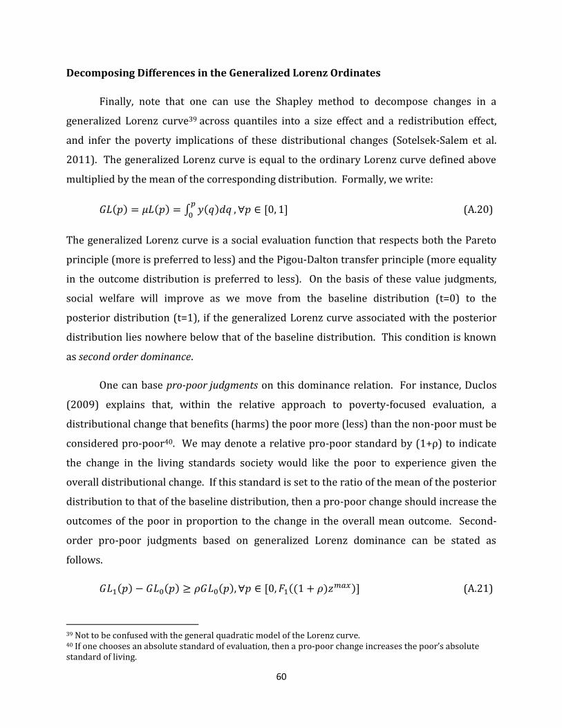
60

Decomposing Differences in the Generalized Lorenz Ordinates

Finally, note that one can use the Shapley method to decompose changes in a

generalized Lorenz curve39 across quantiles into a size effect and a redistribution effect,

and infer the poverty implications of these distributional changes (Sotelsek-Salem et al.

2011). The generalized Lorenz curve is equal to the ordinary Lorenz curve defined above

multiplied by the mean of the corresponding distribution. Formally, we write:

(A.20)

The generalized Lorenz curve is a social evaluation function that respects both the Pareto

principle (more is preferred to less) and the Pigou-Dalton transfer principle (more equality

in the outcome distribution is preferred to less). On the basis of these value judgments,

social welfare will improve as we move from the baseline distribution (t=0) to the

posterior distribution (t=1), if the generalized Lorenz curve associated with the posterior

distribution lies nowhere below that of the baseline distribution. This condition is known

as second order dominance.

One can base pro-poor judgments on this dominance relation. For instance, Duclos

(2009) explains that, within the relative approach to poverty-focused evaluation, a

distributional change that benefits (harms) the poor more (less) than the non-poor must be

considered pro-poor40. We may denote a relative pro-poor standard by (1+ρ) to indicate

the change in the living standards society would like the poor to experience given the

overall distributional change. If this standard is set to the ratio of the mean of the posterior

distribution to that of the baseline distribution, then a pro-poor change should increase the

outcomes of the poor in proportion to the change in the overall mean outcome. Second-

order pro-poor judgments based on generalized Lorenz dominance can be stated as

follows.

(A.21)

39 Not to be confused with the general quadratic model of the Lorenz curve. 40 If one chooses an absolute standard of evaluation, then a pro-poor change increases the poor’s absolute standard of living.

61

Where F1(∙) is the posterior distribution function and zmax the maximum level of the

poverty line. When the relative standard is set to the ratio of the outcome means, then

condition (A.21) is equivalent to having the Lorenz curve of the posterior distribution

located above that of the baseline distribution over the relevant range of p.

Given the overall judgment represented by (A.21), one might be interested in

identifying the contribution of the size effect and that of the redistribution effect into that

overall change. The left-hand side of (A.21) can be written as follows.

(A.22)

Following the same logic as in the case of poverty measures, we compute the size effect as:

(A.23)

The corresponding redistribution effect is:

(A.24)

Atkinson (1987) establishes a relationship between second order dominance and

poverty reduction. In particular, he proves that if , then we know that posterior

outcome distribution has less poverty than the baseline distribution for all poverty lines

and all poverty measures defined by equation (27) in the text that respect the transfer

principle. This provides us with a basis for tracking the poverty implications of the size

effect or the redistribution effect. By definition, . In other

word, the ordinates of the end-period generalized Lorenz curve are obtained by adding the

difference in ordinates to the corresponding ordinates of the baseline generalized Lorenz

curve. Following Sotelsek-Salem et al. (2011), instead of adding the total difference, we

add only the redistribution effect to obtain the following intermediate generalized Lorenz

curve.

(A.25)

62

If this intermediate curve dominates the baseline curve, in order words if the redistribution

effect is positive for all p, then the redistribution effect reduces poverty as measured by all

members of the additively separable class that respect the transfer principle.

Note that the pro-poor test presented in (A.21) can be restated as follows.

(A.26)

This suggests that the redistribution effect will be relatively pro-poor if the following

condition holds.

(A.27)

In other words,

. This test for second-order relative

pro-poorness entails a comparison of growth rates of the cumulative income of proportions

p of the poorest to the standard rate ρ. An equivalent test is based on the so-called three I’s

of poverty (TIP) curve of Jenkins and Lambert (1997), which is obtained by partially

cumulating individual contributions to overall poverty from the poorest individual to the

richest, and normalizing.

II. Within-Group and Population Shift Effects

The application of the decomposition methods described above to the class of

additively decomposable poverty measures allows the analyst to decompose changes in

poverty over time into an effect due to changes in within-group poverty and another due to

population shifts. Let the total population of a given country be partitioned exhaustively

into m socioeconomic groups. Let wkt be the share of population in group k at time t for

t=0, 1, and Pkt the level of poverty in that group at the same time. For additively

decomposable poverty measures, overall poverty at time t can be written as follows.

(A.28)

The change in aggregate poverty over time can now be written as follows.

(A.29)

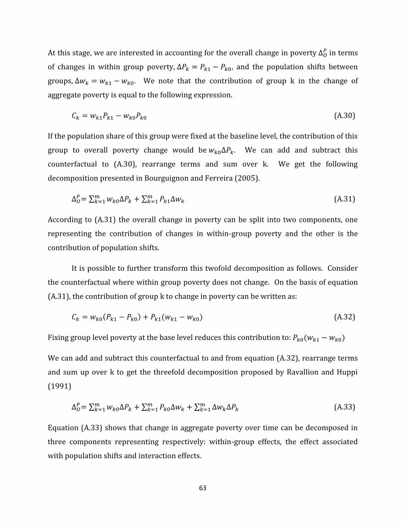
63

At this stage, we are interested in accounting for the overall change in poverty in terms

of changes in within group poverty, , and the population shifts between

groups, . We note that the contribution of group k in the change of

aggregate poverty is equal to the following expression.

(A.30)

If the population share of this group were fixed at the baseline level, the contribution of this

group to overall poverty change would be . We can add and subtract this

counterfactual to (A.30), rearrange terms and sum over k. We get the following

decomposition presented in Bourguignon and Ferreira (2005).

(A.31)

According to (A.31) the overall change in poverty can be split into two components, one

representing the contribution of changes in within-group poverty and the other is the

contribution of population shifts.

It is possible to further transform this twofold decomposition as follows. Consider

the counterfactual where within group poverty does not change. On the basis of equation

(A.31), the contribution of group k to change in poverty can be written as:

(A.32)

Fixing group level poverty at the base level reduces this contribution to:

We can add and subtract this counterfactual to and from equation (A.32), rearrange terms

and sum up over k to get the threefold decomposition proposed by Ravallion and Huppi

(1991)

(A.33)

Equation (A.33) shows that change in aggregate poverty over time can be decomposed in

three components representing respectively: within-group effects, the effect associated

with population shifts and interaction effects.

64

Shorrocks (1999) also shows that the Shapley principle applies to this situation as

well and leads to the following twofold decomposition of change in aggregate poverty over

time.

(A.34)

65

References

Angrist Joshua D. and Pischke Jörn-Steffen. 2009. Mostly Harmless Econometrics: An

Empiricist’s Companion. Princeton: Princeton University Press.

Atkinson, A. B. 1987. On the Measurement of Poverty. Econometrica, Vol. 55, No.4: 749-

764.

Autor David H. 2009. Lecture Note: Self-Selection The Roy Model. Department of

Economics, MIT, http://econ-www.mit.edu/files/4092

Bauer Thomas K. and Sinning Mathias. 2008. An Extension of the Blinder-Oaxaca

Decomposition to Nonlinear Models. Advances in Statistical Analysis, Vol. 92,

No. 2 :197-206.

Bhaumik Sumon Kumar, Gang Ira N. And Yun Myeong-Su. 2006. A Note on Decomposing

Differences in Poverty Incidence Using Regression Estimates: Algorithm and

Example. IZA Discussion Paper No. 2262.

Bitler Marianne P., Gelbach Jonah B., and Hoynes Hilary W. 2006. What Mean Impacts

Miss: Distributional Effects of Welfare Reform Experiments. American Economic

Review, Volume 96, No. 4: 988-1012.

Blinder Alan S. 1973. Wage Discrimination: Reduced Form and Structural Estimates. The

Journal of Human Resources, Vol. 8, No.4: 436-455.

Blundell Richard and Macurdy Thomas. 1999. Labor Supply: A Review of Alternative

Approaches. In Orley Ashenfelter and David Card (eds), Handbook of Labor

Economics , Vol. 3: 1559-1695. New York: Elsevier Science.

Bourguignon François, Ferreira Francisco H. G. and Leite Phillippe G. . 2008. Beyond

Oaxaca-Blinder : Accounting for Differences in Households Income Distributions.

Journal of Economic Inequality, Vol. 6, No.2, 117-148

Bourguignon François and Spadaro Amedeo. 2006. Microsimulation as a Tool for

Evaluating Redistribution Policies. Journal of Economic Inequality, 4: 77-106.

Bourguignon François and Ferreira Francisco H. G. 2005. Decomposing Changes in the

Distribution of Household Incomes: Methodological Aspects. In François

Bourguignon, Francisco H.G. Ferreira and Nora Lustig (eds), The

66

Microeconomics of Income Distribution Dynamics in East Asia and Latin

America, pp. 17-46 Washington, D.C.: The World Bank.

Bourguignon François, Ferreira Francisco H. G. and Lustig Nora 2005. Introduction. In

François Bourguignon, Francisco H.G. Ferreira and Nora Lustig (eds), The

Microeconomics of Income Distribution Dynamics in East Asia and Latin

America, pp. 17-46 Washington, D.C.: The World Bank

Bourguignon François, Fournier Martin, and Gurgand Marc. 2004. Selection Bias

Corrections Based on Multinomial Logit Model: Monte-Carlo Comparisons.

DELTA Working Paper No. 2004-20.

Bourguignon François, Fournier M. and Gurgand M. 2001. Fast Development with a Stable

Income Distribution : Taiwan, 1979-1994. Review of Income and Wealth, Series

47, No2 : 139-163.

Bourguignon François and Ferreira Francisco H. G. 2003. Ex Ante Evaluation of Policy

Reforms Using Behavioral Models. In François Bourguignon and Luiz A. Pereira

da Silva (eds), « The Impact of Economic Policies on Poverty and Income

Distribution : Evaluation Techniques and Tools. Washington, D.C. : The World

Bank.

Cahuc Pierre and Zylberberg André. 2004. Labor Economics. Cambridge (Massachusetts):

The MIT Press.

Carneiro Pedro, Hansen Karsten T. and Heckman James J. 2002. Removing the Veil of

Ignorance in Assessing the Distributional Impacts of Social Policies. Institute for

the Study of Labor (IZA) Discussion Paper No. 453.

Chenery Hollis, Ahluwalia Montek S., Bell C.L. G., Duloy John H. and Jolly Richard. 1974.

Redistribution with Growth: Policies to Improve Income Distribution in

Developing Countries in the Context of Economic Growth. Oxford: Oxford

University Press.

Cogneau Denis and Robilliard Anne-Sophie. 2008. Simulating Targeted Policies with

Macro Impact: Poverty Alleviation Policies in Madagascar. In François

Bourguignon, Maurizio Bussolo and Luiz A. Pereira da Silva (eds), “The Impact of

Macroeconomic Policies on Poverty and Income Distribution: Macro-Micro

Evaluation Techniques and Tools”. Washington, D.C. : The World Bank.

67

Cogneau Denis and Robilliard Anne-Sophie. 2007 Growth, Distribution, and Poverty in

Madagascar: Learning from a Microsimulation Model in a Genberal Equilibrium

Framework. In Amedeo Spadaro (ed), “Microsimulation as a Tool for the

Evaluation of Public Policies: Methods and Applications”. Bilbao: Fundacion

BBVA.

Coulombe Harold and McKay Andrew. 1996. Modeling Determinants of Poverty in

Mauritania. World Development, Vol. 24. No.6: 1015-1031.

Creedy John and Duncan Alan. 2002. Behavioural Microsimulation with Labour Supply

Responses. Journal of Economic Surveys, Vol. 16, No. 1: 1-40.

Datt Gaurav. 1998. Computational Tools for Poverty Measurement and Analysis.

International Food Policy Research Institute (IFPRI), Food Consumption and

Nutrition Division (FCND), Discussion Paper No. 50.

Datt Gaurav and Ravallion Martin. 1992. Growth and Redistribution Components of

Changes in Poverty Measures: a Decomposition with Applications to Brazil and

India in the 1980s. Journal of Development Economics, 38: 275-296.

Deaton, A. 1997. The Analysis of Household Surveys: A Microeconometric Approach to

Development Policy. Baltimore: The John Hopkins University Press.

Deaton Angus and Muellbauer John. 1980. Economics and Consumer Behavior. London:

Cambridge University Press.

DiNardo John, Fortin Nicole and Lemieux Thomas. 1996. Labor Market Institutions and

the Distribution of Wages, 1973-1992 : A Semi-Parametric Approach.

Econometrica, Vol, 64, No. 5 : 1001-1044.

Duclos Jean-Yves. 2009. What is “Pro-Poor”? Social Choice and Welfare, 32 : 37-58.

Duncan Alan. 1993. Labour Supply Decisions and Non-Convex Budget Sets: The Case of

National Insurance Contribution in U.K. In Alberto Heimler and Daniele Meulders

(eds), Empirical Approaches to Fiscal Policy Modelling. (137-162). London :

Chapman & Hall.

Elder Todd E., Goddeeris John H. and Haider Steven J. 2010. Unexplained Gaps and

Oaxaca-Blinder Decompositions. Labour Economics 17: 284-290.

Essama-Nssah B. 1997. Impact of Growth and Distribution on Poverty in Madagascar.

Review of Income and Wealth, Series 43, No.2 : 239-252.

68

Essama-Nssah B. and Lambert Peter J. 2011. Influence Functions for Distributional

Statistics. Society for the Study of Economic Inequality (ECINEQ), Working Paper

No. 2011-236.

Essama-Nssah B. and Bassole Leandre. 2010. A Counterfactual Analysis of the Poverty

Impact of Economic Growth in Cameroon. World Bank Policy Research Working

Paper No. 5249.

Essama-Nssah, B. and Lambert Peter J. 2009. Measuring Pro-Poorness: a Unifying

Approach with New Results. Review of Income and Wealth, Series 55, No.3: 752-

778.

Essama-Nssah B., Bassole Leandre and Paul Saumik. 2010. Accounting for Heterogeneity

in Growth Incidence in Cameroon. World Bank Policy Research Working Paper

5464.

Fairlie Robert W. 2005. An Extension of the Blinder-Oaxaca Decomposition Technique to

Logit and Probit Models. Journal of Economic and Social Measurement, Vol. 30,

No. 4: 305-316.

Ferreira Francisco H.G.: Distributions in Motion: Economic Growth, Inequality and Poverty

Dynamics. 2010. World Bank Policy Research Working Paper No. 5424. The

World Bank, Washington, D.C.

Firpo Sergio, Fortin Nicole and Lemieux Thomas. 2009. Unconditional Quantile

Regressions. Econometrica, Volume 77, No. 3: 953-973 .

Fortin Nicole, Lemieux Thomas and Firpo Sergio. 2011. Decomposition Methods in

Economics. In: Ashenfelter Orley and Card David (eds) Handbook of Labor

Economics, Vol. 4A , pp. 1-102. Northolland, Amsterdam.

Foster James, Greer Joel, and Thorbecke Erik. 1984. A Class of Decomposable Poverty

Measures. Econometrica, Vol. 52, No. 3:761-766.

Glick Peter and Sahn David. 2006. The Demand for Primary Schooling in Madagascar:

Price, Quality and the Choice Between Public and Private Providers. Journal of

Development Economics, Vol. 79, No. 1: 118-145.

Grimm Michael. 2005. Educational Policies and Poverty Reduction in Cote d’Ivoire.

Journal of Policy Modeling, Vol, 27, No. 2 : 231-247.

69

Grimm Michael. 2004. A Decomposition of Inequality and Poverty Changes in the Context

of Macroeconomic Adjustemnt : A Microsimulation Study for Cote d’Ivoire. In,

Growth, Inequality and Poverty : A.F. Shorrocks and R. van der Hoeven (eds) :

Prospects for Pro-Poor Economic Development. Oxford : Oxford University

Press.

Hall, Bronwyn H. 2002. Notes on Sample Selection Models (mimeo).

Heckman, James J. 1979. Sample Selection Bias as a Specification Error. Econometrica, Vol.

47, No.1: 153-161.

Heckman, James J. 1976. The Common Structure of Statistical Models of Truncation,

Sample Selection and Limited Dependent Variables and a Simple Estimator fro

such Models. Annals of Economic and Social Measurement, Vol.5, No. 4: 475-492.

Heckman James J. and Navarro-Lozano Salvador. 2004. Using Matching, Instrumental

Variables, and Control Functions to Estimate Economic Choice Models. The

Review of Economics and Statistics, Vol. 86, No. 1: 30-57.

Heckman James J. and Smith Jeffrey. A. 1995. Assessing the Case of Social Experiments.

Journal of Economic Perspectives, Vol. 9, Issue 2:85-110.

Heckman James J. and Honoré Bo E. 1990. The Empirical Content of the Roy Model.

Econometrica, Vol. 58. No. 5 : 1121-1149.

Heckman James J. and Sedlacek Guilherme. 1985. Heterogeneity, Aggregation, and Market

Wage Functions : An Empirical Model of Self-Selection in the Labor Market. The

Journal of Political Economy, Vol. 93, No.6 :1077-1125.

Heinrichs Jutta and Kennedy Peter. 2007. A Computational Trick for Calculating the

Blinder-Oaxaca Decomposition and Its Standard Error. Economics Bulletin, Vol.

3, No. 66: 1-7.

Huppi Monika and Ravallion Martin. 1991. The Sectoral Structure of Poverty During an

Adjustement Period : Evidence for Indonesia in the Mid-1980s. World

Development, Vol. 9, No.12 :1653-1678.

Jann Ben. 2008. A Stata Implementation of the Blinder-Oaxaca Decomposition. ETH

(Eidgenössische Technische Hochschule) Zurich Sociology Working Paper No.5

(Swiss Federal Institute of Technology).

70

Juhn Chinhui, Murphy Kevin M. and Brooks Pierce. 1993. Wage Inequality and the Rise of

Returns to Skill. Journal of Political Economy, Vol. 101, No.3 : 410-442.

Juhn Chinhui, Murphy Kevin M. and Brooks Pierce. 1991. Accounting for the Slowdown in

Black-White Wage Convergence. In Marvin H. Kosters (ed), Workers and their

Wages : Changing Patterns in the United States. Washington DC : American

Enterprise Institute.

Kakwani Nanak. 2000. On Measuring Growth and Inequality Components of Poverty with

Application to Thailand. Journal of Quantitative Economics, Vol.16, No. 1 :67-79.

Kline Patrick. 2010. Blinder-Oaxaca as a Reweighting Estimator. Department of

Economics, University of California at Berkeley, Mimeo.

Kolenikov Stanislav and Shorrocks Anthony. 2005. A Decomposition Analysis of Regional

Poverty in Russia. Review of Development Economics, Vol. 9, No. 1 :25-46.

Kraay Aart. 2006. When is Growth Pro-Poor ? Evidence from a Panel of Countries. Journal

of Development Economics, 80 : 198-227.

Kunze Astrid. 2008. Gender Wage Gap Studies : Consistency and Decomposition. Empirical

Economics, No. 35 : 63-76.

Lambert, Peter J. 2001. The Distribution and Redistribution of Income. Manchester:

Manchester University Press.

Lee, Lung-Fei. 1983. Generalized Econometric Models with Selectivity. Econometrica, Vol.

51, No. 2:507-512.

Leite Phillippe G. and Fruttero Anna. 2010. Toolkit on Simulating the Impact of

Conditional Cash Transfer Programs www.worldbank.org/safetynets.

Leite Phillippe G., Sanchez Alan, and Laderchi Caterina R. 2009. The Evolution in Urban

Inequality in Ethiopia. Washington, DC. : The World Bank (mimeo).

Machado J. and Mata J. 2005. Counterfactual Decomposition of Changes in Wage

Distributions Using Quantile Regression. Journal of Applied Econometrics 20

(4): 445-465.

Maddala, G. S. 1983. Limited-Dependent and Qualitative Variables in Econometrics.

Cambridge: Cambridge University Press.

71

Melly Blaise. 2005. Decomposition of Differences in Distribution Using Quantile

Regression. Labour Economics, 12: 577-590.

Milgrom Paul. 2004. Putting Auction Theory to Work. Cambridge: Cambridge University

Press.

Moulin, Hervé. 2003. Fair Division and Collective Welfare. Cambridge, Massachusetts: The

MIT Press.

Neuman Shoshana and Oaxaca Ronald L. 2004. Wage Decompositions with Selectivity-

Corrected Wage Equations: A Methodological Note. Journal of Economic

Inequality, 2: 3-10.

Nguyen Binh T., Albrecht James W., Vroman Susan B. and Westbrook M. Daniel. 2007. A

Quantile Regression Decomposition of Urban-Rural Inequality in Vietnam.

Journal of Development Economics 83: 466-490.

Nielsen Skyt Helena. 1998. Discrimination and Detailed Decomposition in a Logit Model.

Economics Letters, 61: 115-120.

Oaxaca Ronald L. 1973. Male-Female Wage Differentials in Urban Labor Markets.

International Economic Review, Vol. 14, No.3: 693-709.

Rapoport Anatol. 1999. Two-Person Game Theory. Mineola (New York): Dover

Publications.

Ravallion Martin. 2001. Growth, Inequality and Poverty: Looking Beyond Averages. World

Development, Vol 29: No. 11: 1803-1815.

Ravallion Martin. 2000. On Decomposing Changes in Poverty into “Growth” and

“Redistribution” Components . Journal of Quantitative Economics, Vol. 16, No. 1:

105-118.

Ravallion Martin and Chen Shaohua. 2003. Measuring Pro-Poor Growth. Economic Letters

78, 93-99.

Ravallion Martin and Huppi Monika. 1991. Measuring Changes in Poverty: A

Methodological Case Study of Indonesia during an Adjustment Period. The World

Bank Economic Review, Vol.5, No5:57-82.

72

Rosenbaum Paul and Rubin Donald. 1983. The Central Role of the Propensity Score in

Observational Studies for Causal Effects. Biometrika, 1983, Vol, 70, No. 1: 41-55.

Rothe Christoph. 2010. Decomposing Counterfactual Distributions. Toulouse School of

Economics, mimeo.

Roy A. 1951. Some Thoughts on the Distribution of Earnings. Oxford Economic Papers, 3:

135-146.

Salanié Bernard. 2003. The Economics of Taxation. Cambridge (Massachusetts): The MIT

Press.

Schmertmann, C. P. 1994. Selectivity Bias Correction Methods in Polychotomous Sample

Selection Models. Journal of Econometrics, Vol. 60:101-132.

Shorrocks A. F. 1999. Decomposition Procedures for Distributional Analysis: A Unified

Framework Based on Shapley Value. University of Essex and Institute for Fiscal

Studies, mimeo.

Silverman, B.W. 1986. Density Estimation for Statistics and Data Analysis. London:

Chapman and Hall.

Sinning Mathias, Hahn Markus and Bauer Thomas K. 2008. The Blinder-Oaxaca

Decomposition for Nonlinear Models. The Stata Journal, Vol. 8, No.4: 480-92.

Sotelsek-Salem Daniel, Ahamdanech-Zarco Ismael, and Bishop John A. 2011. Dominance

Testing for “Pro-Poor” Growth with an Application to European Growth.

Empirical Economics (forthcoming).

Spadaro Amedeo. 2007. Microsimulation as a Tool for the Evaluation of Public Policies. In

Amedeo Spadaro (ed), “Microsimulation as a Tool for the Evaluation of Public

Policies: Methods and Applications”. Bilbao: Fundacion BBVA.

Todd Petra E. 2008. Evaluating Social Programs with Endogenous Program Placement and

Selection of the Treated. In Schultz T.P. and Strauss J. (eds), Handbook of

Development Economics, Vol. 4.:3847-3894

Train Kenneth E. 2009. Discrete Choice Methods with Simulation. Cambridge: Cambridge

University Press (Second Edition).

Train Kenneth E. and Wilson Wesley W. 2008. Estimation on Stated-Preference

Experiments Constructed from Revealed-Preference Choices. Transportation

Research Part B, Vol, 42, Issue 3: 191-203.

73

Varian Hal R. 1984. Microeconomic Analysis. New York: Norton & Company (second

edition)

Von Mises R. 1947. On the Asymptotic Distribution of Differentiable Statistical Functions.

The Annals of Mathematical Statistics, 18, 309-348.

Wilcox Rand R.. 2005. Introduction to Robust Estimation and Hypothesis Testing (Second

Edition). Elsevier, Amsterdam.

World Bank. 2005. World Development Report 2006: Equity and Development.

Washington, D.C. The World Bank and Oxford University Press.

World Bank . 1990. World Development Report 1990: Poverty. Washington, D.C.: The

World Bank.

World Bank. 1978. World Development Report, 1978. Washington, D.C.: The World Bank.

Young, H. Peyton. 1994. Equity: In Theory and Practice. Princeton: Princeton University

Press.

Yun Myeong-Su. 2009. Wage Differentials, Discrimination and Inequality: A Cautionary

Note on the Juhn, Murphy and Pierce Decomposition Method. Scottish Journal of

Political Economy, Vol. 56, No. 1: 114-122

Yun Myeong-Su. 2005. A Simple Solution to the Identification Problem in Detailed Wage

Decompositions. Economic Inquiry, Vol. 43, No. 4: 766-772.

Yun Myeong-Su. 2004. Decomposing Differences in the First Moments. Economics Letters,

Vol. 82, No. 2:275-280.

B. Essama-Nssah: Identification of Sources of Variation in Poverty Outcomes (Tuesday, January 17, 2012)