Identification of High-Tech Motion Systems:

An Active Vibration Isolation Benchmark

Robbert Voorhoeve, ⇤ Annemiek van Rietschoten, ⇤

Egon Geerardyn, ⇤⇤ Tom Oomen ⇤

⇤Eindhoven University of Technology. Department ME, CST group.

Eindhoven, The Netherlands (e-mail: r.j.voorhoeve@tue.nl).

⇤⇤Vrije Universiteit Brussel. Department ELEC. Brussels, Belgium.

Abstract: The benchmark Active Vibration Isolation System (AVIS) in this paper is a complexhigh-tech industrial system used in vibration and motion control applications. The system iscomplex in the sense of high order flexible dynamics and multiple inputs and outputs. The aimof this benchmark is to compare di↵erent black box, linear time invariant system identificationalgorithms. Di↵erent large data sets are provided, enabling the use of both frequency domainand time domain identification approaches. The idea of the benchmark is to investigate bothmodel accuracy and numerical reliability of the computational steps. Several reference solutionsare provided, which demonstrate the challenging aspects of this benchmark already in the single-input single-output case. The benchmark data and additional info are available on the website ofTom Oomen 1.

1. INTRODUCTION

The aim of this Active Vibration Isolation System (AVIS)benchmark is to compare the capability of di↵erent blackbox, linear time invariant identification techniques tomodel complex industrial systems. The main idea is thatan industrial high-tech system, characterized by highlyaccurate sensors & actuators, over-actuation and a highdegree of active control, automatically constitutes a prac-tically relevant setup on which to test identification algo-rithms. The presented benchmark system is complex inthe sense of high order, lightly damped dynamics with asignificant dimension in terms of inputs and outputs.The proposed benchmark is based on a mechanical systemthat has applications in motion and vibration control. Inthe near future the requirements for motion and vibrationcontrol will become even tighter. To meet these futuredemands, it is envisaged in Oomen et al. (2014b, SectionI.C) that active control of flexible dynamics is required,including the use of additional actuators and sensors andinferential control. This implies that the number of inputsand outputs is likely to increase, as well as the orderof the relevant flexible dynamics. As a result, a model-based control approach (van de Wal et al., 2002) based onparametric models is a natural approach for a systematiccontrol design for such complex multivariable systems.Although many control applications for motion systemsare reported in the literature, there is a strong indicationthat the modeling task still poses a major challenge. Sys-tem identification is the natural approach for such systems,since it is inexpensive, fast, and accurate due to the almostinfinite freedom in the design of experiments. However,there are indications that it is unclear for practitionerswhat method to prefer and choose from the large amountof approaches available.These indications are at least threefold. First, most motionsystems are still tuned manually using non-parametric

1http://www.dct.tue.nl/toomen/avis/avis.html

models, see Van de Wal et al. (2002), Butler (2011).Second, it is explicitly indicated in earlier overviews of themotion control field, e.g., already in Steinbuch and Norg(1998, Section 4.2, limitations of tools), that modelingtools are not readily available. Third, besides the fact thatmany system identification approaches with di↵erent crite-ria have been developed, a significant number of results ad-dressing issues with the numerical implementation of thesemethods have been developed, including frequency scaling(Pintelon and Kollar, 2005), amplitude scaling (Hakvoortand Van den Hof, 1994), the use of classical orthonormalpolynomials and orthogonal rational functions (Heubergeret al., 2005, Section 3.1), (Ninness et al., 2000), (Ninnessand Hjalmarsson, 2001), and more recently the use of or-thonormal basis functions with respect to a discrete data-based inner product (Bultheel et al., 2005), (Van Herpenet al., 2014). Related numerical issues are also seen insubspace identification, see e.g., Verdult et al. (2002) andChiuso and Giorgio (2004).

The proposed benchmark system is an Active VibrationIsolation System (AVIS), which is selected for its appli-cation interest, applicability and relevance, and challenge.Regarding application interest, these systems are used indiverse fields, ranging from precision equipment such aslithography and scanning tunneling and atomic force mi-croscopy to vehicles, and their control is an active researchtopic by itself, see e.g., Landau et al. (2013). Regardingapplicability and relevance, the considered AVIS is open-loop stable. This is in sharp contrast to typical high-performance motion systems that require closed-loop op-eration to stabilize the rigid-body behavior. As such, theapproach eliminates issues that could arise due to closed-loop operation, including potential bias and the influenceof the controller on the resulting model, enabling a mean-ingful and unambiguous evaluation of many available iden-tification approaches. Regarding the challenge component,the system has 8 inputs and 6 outputs with high-orderflexible dynamics over a large dynamic range, leading to a

Preprints of the 17th IFAC Symposium on System Identification

Beijing International Convention Center

October 19-21, 2015. Beijing, China

Copyright © IFAC 2015 1250

x y

z

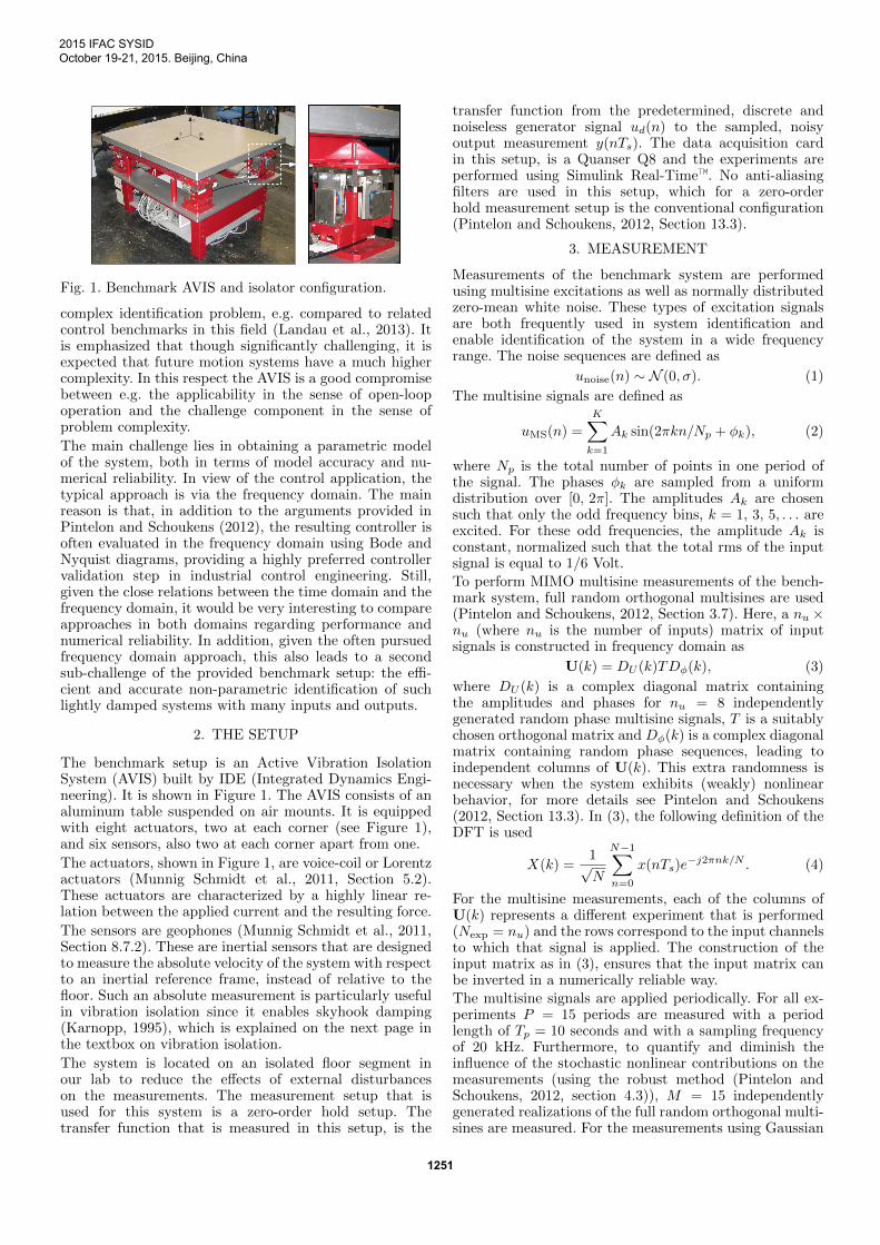
Fig. 1. Benchmark AVIS and isolator configuration.

complex identification problem, e.g. compared to relatedcontrol benchmarks in this field (Landau et al., 2013). Itis emphasized that though significantly challenging, it isexpected that future motion systems have a much highercomplexity. In this respect the AVIS is a good compromisebetween e.g. the applicability in the sense of open-loopoperation and the challenge component in the sense ofproblem complexity.The main challenge lies in obtaining a parametric modelof the system, both in terms of model accuracy and nu-merical reliability. In view of the control application, thetypical approach is via the frequency domain. The mainreason is that, in addition to the arguments provided inPintelon and Schoukens (2012), the resulting controller isoften evaluated in the frequency domain using Bode andNyquist diagrams, providing a highly preferred controllervalidation step in industrial control engineering. Still,given the close relations between the time domain and thefrequency domain, it would be very interesting to compareapproaches in both domains regarding performance andnumerical reliability. In addition, given the often pursuedfrequency domain approach, this also leads to a secondsub-challenge of the provided benchmark setup: the e�-cient and accurate non-parametric identification of suchlightly damped systems with many inputs and outputs.

2. THE SETUP

The benchmark setup is an Active Vibration IsolationSystem (AVIS) built by IDE (Integrated Dynamics Engi-neering). It is shown in Figure 1. The AVIS consists of analuminum table suspended on air mounts. It is equippedwith eight actuators, two at each corner (see Figure 1),and six sensors, also two at each corner apart from one.The actuators, shown in Figure 1, are voice-coil or Lorentzactuators (Munnig Schmidt et al., 2011, Section 5.2).These actuators are characterized by a highly linear re-lation between the applied current and the resulting force.The sensors are geophones (Munnig Schmidt et al., 2011,Section 8.7.2). These are inertial sensors that are designedto measure the absolute velocity of the system with respectto an inertial reference frame, instead of relative to thefloor. Such an absolute measurement is particularly usefulin vibration isolation since it enables skyhook damping(Karnopp, 1995), which is explained on the next page inthe textbox on vibration isolation.The system is located on an isolated floor segment inour lab to reduce the e↵ects of external disturbanceson the measurements. The measurement setup that isused for this system is a zero-order hold setup. Thetransfer function that is measured in this setup, is the

transfer function from the predetermined, discrete andnoiseless generator signal ud(n) to the sampled, noisyoutput measurement y(nTs). The data acquisition cardin this setup, is a Quanser Q8 and the experiments areperformed using Simulink Real-Time™. No anti-aliasingfilters are used in this setup, which for a zero-orderhold measurement setup is the conventional configuration(Pintelon and Schoukens, 2012, Section 13.3).

3. MEASUREMENT

Measurements of the benchmark system are performedusing multisine excitations as well as normally distributedzero-mean white noise. These types of excitation signalsare both frequently used in system identification andenable identification of the system in a wide frequencyrange. The noise sequences are defined as

unoise

(n) ⇠ N (0,�). (1)

The multisine signals are defined as

uMS

(n) =KX

k=1

Ak sin(2⇡kn/Np + �k), (2)

where Np is the total number of points in one period ofthe signal. The phases �k are sampled from a uniformdistribution over [0, 2⇡]. The amplitudes Ak are chosensuch that only the odd frequency bins, k = 1, 3, 5, . . . areexcited. For these odd frequencies, the amplitude Ak isconstant, normalized such that the total rms of the inputsignal is equal to 1/6 Volt.To perform MIMO multisine measurements of the bench-mark system, full random orthogonal multisines are used(Pintelon and Schoukens, 2012, Section 3.7). Here, a nu ⇥nu (where nu is the number of inputs) matrix of inputsignals is constructed in frequency domain as

U(k) = DU (k)TD�(k), (3)

where DU (k) is a complex diagonal matrix containingthe amplitudes and phases for nu = 8 independentlygenerated random phase multisine signals, T is a suitablychosen orthogonal matrix and D�(k) is a complex diagonalmatrix containing random phase sequences, leading toindependent columns of U(k). This extra randomness isnecessary when the system exhibits (weakly) nonlinearbehavior, for more details see Pintelon and Schoukens(2012, Section 13.3). In (3), the following definition of theDFT is used

X(k) =1pN

N�1X

n=0

x(nTs)e�j2⇡nk/N . (4)

For the multisine measurements, each of the columns ofU(k) represents a di↵erent experiment that is performed(N

exp

= nu) and the rows correspond to the input channelsto which that signal is applied. The construction of theinput matrix as in (3), ensures that the input matrix canbe inverted in a numerically reliable way.The multisine signals are applied periodically. For all ex-periments P = 15 periods are measured with a periodlength of Tp = 10 seconds and with a sampling frequencyof 20 kHz. Furthermore, to quantify and diminish theinfluence of the stochastic nonlinear contributions on themeasurements (using the robust method (Pintelon andSchoukens, 2012, section 4.3)), M = 15 independentlygenerated realizations of the full random orthogonal multi-sines are measured. For the measurements using Gaussian

2015 IFAC SYSID

October 19-21, 2015. Beijing, China

1251

Vibration isolation aims to suppress the influence of external disturbances on the payload. These external disturbances can beseparated in two classes, Fd1, acting on the floor and Fd2, acting directly on the payload. See Fig. 3 for a schematic model of the AVIS.

C Pu

Fd

y

�

Fig. 2. Simple feedback interconnectionfor active vibration isolation.

Floor

y

Fd1

Fd2

Payload

C

Fig. 3. Traditional setup, measuring thevelocity relative to the floor.

“Sky”

yC Fd

1

Fd2

Payload

Floor

Fig. 4. Skyhook damping of the AVIS, us-ing an absolute velocity measurement.

In passive vibration isolation the challenge is to design suspension characteristics (modeled by a spring and damper in Fig. 3), suchthat the disturbances Fd1 and Fd2 are optimally suppressed. To suppress the floor disturbances Fd2, a soft suspension is desired sincethis maximizes the frequency range in which the floor and AVIS are decoupled, leading to good isolation of the AVIS with respect tofloor disturbances. However, to suppress the system disturbances Fd1, a sti↵ suspension is desired because this minimizes the deflectioncaused by such a disturbance. Hence, there is a clear trade-o↵ in passive vibration isolation.In active vibration isolation, the suppression of external disturbances is enhanced through active feedback control, see Fig. 2. Onepossibility is to measure and actively control the velocity of the system with respect to the floor, as shown in Fig. 3. In this configurationhowever, the controller can be interpreted as an extra suspension element between the floor and the AVIS. This means the same trade-o↵as in passive vibration isolation exists between the suppression of Fd1 and Fd2.If a measurement is available of the absolute velocity of the system, so-called skyhook damping can be used. The name skyhookdamping references the interpretation of the controller as a suspension element (damper) between the AVIS and the fixed world or“sky”, see Fig. 4. This e↵ectively eliminates the trade-o↵ between the suppression of floor disturbances and suppression of systemdisturbances, since they are both suppressed by a strong coupling between the AVIS and the (disturbance free) fixed world. In thiscase, a high control bandwidth is thus desired to attenuate both Fd1 and Fd2.

−0.75

−0.5

−0.25

0

0.25

0.5

0.75

0 4000 8000

u1 [

V]

counts0 10 20

T [s]

−2

−1

0

1

2

0 4000 8000

y1 [

V]

counts0 10 20

T [s]

Fig. 5. Timeseries and histograms of two periods of multi-sine input and an output signals.

noise sequences as inputs, again an nu ⇥ nu input matrixis constructed as in (3), however the initial nu = 8 fre-quency domain signals which define DU (k) are the Fouriercoe�cients of the Gaussian noise sequences instead of themultisines. For each of the noise experiments, the excita-tion signals were applied for 300 seconds. For an overview,see Table 1.

In Figure 5, the time-series and histograms are shownof the first input and output for two periods of themultisine excitation. From these figures, it can be seenthat the amplitude distribution of the multisine signalsapproximates a Gaussian distribution, which is due to theuse of random phases.

Figure 6 shows the frequency domain spectra of thesame input and output data as seen in Figure 5. Theinput spectrum clearly equals the designed deterministicamplitude spectrum for the excited frequencies and showsno excitation for the non-excited frequencies. The outputspectrum already reveals some of the system’s amplitudebehavior and confirms that the system contains a large

Table 1. Overview of conducted experiments.

Nexp real. M periods P Tp [s] Ttot [s]Multisine 8 15 15 10 18000Noise 8 1 1 300 2400

Fig. 6. Frequency domain amplitudes of two periods ofmultisine input and an output signals

number of lightly damped modes, which will become clearin Figure 7. The output spectrum also shows a distinctionbetween the excited and non-excited lines, however thisdistinction is not as sharp as in the input spectrum. Thiscan be attributed to measurement noise and non-linearitiesin the system. Next, a non-parametric characterizationof the frequency response of the system is performed toreduce and quantify the influence of these phenomena.

4. NON-PARAMETRIC IDENTIFICATION

As an intermediate step in system identification, a non-parametric model can be used. This provides valuableinsight in the system behavior and also provides a meansfor data reduction. In this section, the frequency responsematrix of the system is estimated using the multisinemeasurements described in section 3.

2015 IFAC SYSID

October 19-21, 2015. Beijing, China

1252

Real-life systems will always exhibit some non-linear be-havior, therefore the frequency response matrix will atbest be a linear approximation of the system behavior. Toobtain a good linear approximation, the so-called robustmethod for estimating the best linear approximation isused, see Pintelon and Schoukens (2012, Sections 4.3.1 &7.3.6). Note that this best linear approximation can stilldepend on certain aspects of the applied input signal suchas its rms value and DC o↵set. Here, a self-containedsummary of this method for estimating the best linearapproximation is described.For each realization m, experiment e and period p, any ⇥ 1 vector of output signals (with signal length N =fsTp) is measured. These are first transformed to thefrequency domain using the DFT defined by (4). Theoutput observations are described by

Y (k) = GBLA

(⌦k)U(k) + VY (k) + Ys(k) + TY (⌦k), (5)

where GBLA

(⌦k) is the best linear approximation of thesystem, U(k) is the DFT of the input signal, VY (k) isthe disturbing noise on the output observations, Ys(k)is the stochastic non-linear contribution and TY (⌦k) isthe transient response (or leakage) term. The influence ofall three of these disturbance terms should be mitigatedand/or quantified during non-parametric identification.The transient term TY (⌦k) is mitigated by discardingthe measurement data from the first Pt = 5 periods ofthe multisine measurements. Next, the frequency domainsignals are averaged over the remaining P

ss

steady-stateperiods, to mitigate the influence of VY (k)

Y [m,e](k) =1

Pss

PX

p=Pt

+1

Y [m,e,p](k). (6)

To quantify the remaining influence of this noise term, thecovariance of Y [m,e](k) is determined from

Cnoise [m,e]ˆY

(k) =1

Pss

(Pss

� 1)

PX

p=Pt

+1

e[m,e,p]Y (k)e[m,e,p]H

Y (k),

(7)with

e[m,e,p]Y (k) = Y [m,e,p](k)� Y [m,e](k). (8)

Averaging over the multisine periods does not mitigate theinfluence of the stochastic non-linear contributions sincethey have the same periodicity. Therefore, to mitigate andquantify the influence of Ys(k), an averaging step overthe di↵erent realizations m is performed. Since the phasesof the input sinusoids for the di↵erent realizations vary,these varying phases first need to be eliminated before ameaningful average over the realizations can be computed.This is done by first relating the output signals Y [m,e](k)to the inputs signals. The signals of the nu experimentsare combined to form the following matrix of outputs

Y[m]

(k) =hY [m,1](k) Y [m,2](k) . . . Y [m,nu](k)

i. (9)

The matrix of input signals U[m](k) 2 Cnu⇥nu (see (3)) iswritten as:

U[m](k) = D|U |(k)T[m]

\U (k) (10)

where D|U |(k) is a diagonal matrix containing amplitude

information of the input signal and T[m]

\U (k) is a unitarymatrix containing all the phase information of the inputsignals, obtained by rewriting (3) in phasor notation. This

Fig. 7. Magnitude plots for the first 2⇥2 subset of the non-parametric estimate of G

BLA

for the AVIS, includingthe total and noise variances (�

tot

, �noise

respectively).

unitary matrix is used to relate the output signals to theinput signals, allowing the computation of a meaningfulaverage over the M independent realizations, i.e.,

Y[m]

U (k) = Y[m]

(k)T [m]

H

\U (k), (11)

YU (k) =1

M

MX

m=1

Y[m]

U (k). (12)

Next the covariance of this estimate is computed using

C[e]ˆYU(k) =

1

M(M � 1)

MX

m=1

r[m,e]Y (k)r[m,e]H

Y (k), (13)

with

r[m,e]Y (k) = Y

[m]

U [:, e](k)� YU [:, e](k). (14)

The previously obtained covariance estimates of the noiseare used to estimate the noise covariance on YU (k)

Cnoise [e]ˆYU

(k) =1

M2

MX

m=1

Cnoise [m,e]ˆY

(k). (15)

Finally the best linear approximation is computed through

GBLA

(⌦k) = YU (k)D�1

|U |(k). (16)

One final averaging step over the nu experiments yields

CˆYU(k) =

1

nu

nuX

e=1

C[e]ˆYU(k), (17)

and

C noise

ˆYU(k) =

1

nu

nuX

e=1

Cnoise [e]ˆYU

(k). (18)

The total and noise covariances of GBLA

are computed by

CˆGBLA

= cov(vec(GBLA

)) ⇡ (U(k)UH(k))�1 ⌦ CˆYU(k),(19)

where vec(·) denotes the vectorization operator, and

Cnoise

ˆGBLA

⇡ (U(k)UH(k))�1 ⌦ C noise

ˆYU(k). (20)

The results of this procedure for the first 2 ⇥ 2 subset ofthe benchmark setup are shown in Figure 7, showing theresulting best linear approximation as well as the totaland noise standard deviations. These results show thata good signal to noise ratio (> 10dB) is achieved for alarge frequency range and also clearly show the high orderlightly damped dynamics of the system.

2015 IFAC SYSID

October 19-21, 2015. Beijing, China

1253

5. THE BENCHMARK CHALLENGE

5.1 Main benchmark challenge

The main benchmark challenge of this paper is to accu-rately fit a parametric model to the estimated frequencyresponse function (or directly to the time-domain data).A number of metrics are formulated to assess the perfor-mance of di↵erent identification routines.Accuracy metric To assess the accuracy of the obtainedmodel, the value of the sampled maximum likelihood costfunction is used, which is defined as:

VML

(G) =mX

k=1

h"ˆGBLA

(⌦k, G)HW (k)"ˆGBLA

(⌦k, G)i2

,

(21)where "

ˆGBLA

(⌦k, G) is given by

"ˆGBLA

(⌦k, G) = vec(GBLA

(⌦k)� Gprop

(⌦k)), (22)

and the weight matrix is defined as

W (k) = C�1

ˆGBLA

(k). (23)

In (22), Gprop

(⌦k) is the linear system (evaluated atfrequency k) that results from a proposed identificationroutine. In this cost function the identified models arecompared with the non-parametric BLA, ideally one wouldwant to compare the identified models with the true model.A true model is however not available and therefore thisnon-parametric BLA which is estimated based on the fulldata-set is used instead.Subsets The cost function (21) is specified for the full 6⇥8MIMO case, but it can readily be reformulated such that asubset of the MIMO problem is considered. Since the fullMIMO case is rather challenging, it is useful to first assessthe performance of identification algorithms on SISO andsmaller MIMO parts of the system before attempting thefull MIMO case. The subsets that are considered for thebenchmark are those using the first [1 : ny,id] output andthe first [1 : nu,id] input channels. It should always beclearly indicated how many inputs and outputs are used.Numerical reliability To assess the numerical reliabilityof the di↵erent identification algorithms, the conditionnumber with respect to L2 (denoted as ) is used. Mostidentification methods solve a linear system of equationsto calculate the fitting parameters or use a matrix de-composition such as SVD or QR as central solution step.The condition number for this central solution step isconsidered for this benchmark. For iterative algorithms theminimum, maximum and geometric mean values over alliterations should be mentioned.Other metrics Additional relevant metrics are the com-putation time (and on what type of machine), to assess thee�ciency of the method, and the order (McMillan degree)of the estimated model as well as the number of modelparameters that were estimated. Table 2 shows an exampleof all the performance metrics for the reference solutionsused in this paper.

5.2 Secondary benchmark challenge

As a secondary benchmark, a non-parametric identifica-tion challenge is formulated. The non-parametric identifi-cation solution shown in section 4 is used as a referencecase. The challenge is to use the least amount of measure-ment data while maintaining a comparable model quality.

Vnon�linear J

non�linear

= @Vnon�linear@✓

V hiiSK

J hiiIV

= 0 )ChiiHAhii✓hi+1i = ChiiHbhii

J hiiSK

=@V

hiiSK

@✓ = 0 )Ahii✓hi+1i = bhii

Iteratively reformulate Iteratively reformulateIVSK

Fig. 8. Graphical depiction of the basic principles behindthe applied SK and IV algorithms.

For example, local modeling techniques (LPM/LRM, seee.g., Geerardyn et al. (2014)) can be used to mitigate thetransient response instead of discarding the measurementdata from the first five periods, reducing the total amountof measurement periods required.To quantify the model quality, the same cost functionis used as in the parametric identification benchmarkof Section 5, except a non-parametric G

prop

(⌦k) is usedinstead of a parametric model. This cost function isonly defined on a discrete frequency grid (see eq. (21)),but for this non-parametric benchmark, a subset of thisfrequency grid can be used. The cost function should thenbe normalized with the total number of frequency binsthat are considered. If an entirely di↵erent frequency gridis obtained then the applied interpolation method shouldbe clearly defined.

6. A REFERENCE SOLUTION

In this section, a reference solution is provided for thebenchmark challenge where the first SISO element of thesystem is considered. This facilitates presentation and al-ready reveals the challenging numerical aspects involved inthe benchmark challenge. For the SISO case, the sampledmaximum likelihood cost function (21) reduces to

VML i,j(✓) :=

mX

k=1

�����G

BLA i,j(⌦k)� G(⌦k, ✓)

�ˆGBLA i,j

(⌦k)

�����

2

, (24)

where

G(⌦, ✓) =N(⌦, ✓)

D(⌦, ✓), (25)

and where N(⌦, ✓) and D(⌦, ✓) are polynomials in theindeterminate ⌦. This cost function is non-linear in theparameters ✓.Two di↵erent algorithms are utilized, the Sanathanan-Koerner (SK) algorithm (Pintelon and Schoukens, 2012,Section 9.8.3) and the Instrumental Variable (IV) algo-rithm (Blom and Van den Hof, 2010). As is shown inFigure 8, these approaches both involve solving a sequenceof linear systems of equations. Note that these approachesneed not converge monotonically, thereby providing addi-tional robustness with respect to local minima.The problem matrices of these algorithms (C,A and b asin Figure 8) depend on the particular parametrization of(25). Here, the following parametrizations are considered:Mon monomials;ScM monomials that are scaled such that the columns of

A and C have a unity 2-norm; andBP block polynomials �i, j that are bi-orthogonal with

respect to the bi-linear form h i, �jiC,A, that theo-

retically yield (CHA) = 1 as introduced by Van Her-pen et al. (2014).

2015 IFAC SYSID

October 19-21, 2015. Beijing, China

1254

Table 2. Benchmark criteria for reference solutions.

Approach min(VML1,1)

min/gmean/max

tcomp

[s]@i5-4670

order/N

par

IV,BP 4.6e5 1/2/4e22 363 100/200

IV,ScM 5.4e5 2e17/2e18/3e19 165 100/200

IV,Mon 1.3e6 9e70/1e154/1e293 231 100/200

SK,ScM 1.5e6 5e9/2e15/6e16 168 100/200

Fig. 9. Fitted models using the IV algorithm with a bi-orthonormal basis (G

IV,BP

) and the SK algorithm withscaled monomials (G

SK,ScM).

In Figures 9 and 10 and Table 2 the results for these refer-ence solutions of the SISO benchmark problem are shown.In Figure 10 it can be seen that only the IV algorithmparameterized with the bi-orthonormal basis functionsconverges within 200 iterations. All the other parametriza-tions used with the IV algorithm have much higher con-dition numbers which clearly influences the convergenceproperties of the algorithm. For the bi-orthonormal basisthe condition number is equal to 1 for most iterations,however at some iterations it spikes, likely due to imple-mentation issues with the algorithm that constructs thesebases. That these numerical issues are already present forthe SISO case shows the challenging numerical aspectsinvolved in this benchmark.

7. DISCUSSION AND OUTLOOK

In this paper, a benchmark is presented which can beused to evaluate LTI system identification techniqueson a complex industrial motion system with high orderlightly damped dynamics. To assess the performance ofavailable and future approaches in the field of linear systemidentification, evaluation criteria for model quality aswell as numerical reliability are formulated. The criterionused to assess model accuracy is the sampled maximumlikelihood cost function defined in (21). To assess thenumerical reliability of the identification algorithms, thecondition number of the central estimation step is used.The reference solution included in this paper shows thechallenging numerical aspects involved in this benchmark.

The benchmark challenge in this paper is focused on theaccurate and reliable identification of a nominal model foran industrial system. The ultimate goal of the system andhence the model is subsequent control design. The controlgoal introduces additional interesting aspects that may beof relevance for future investigation, including

• identification for control using control-relevant criteria;• uncertainty identification for robust control, prelimi-nary ideas have revealed interesting aspects, see Geer-

0 50 100 150 20010

4

105

106

107

108

109

Iteration

VM

L,f

it

1020

10100

10200

0 50 100 150 20010

0

105

1010

1015

Iteration

κ

IV,Mon

IV,ScM

SK,ScM

IV,BP

Fig. 10. Cost function values and conditions numbers duringiterations for the reference solutions.

ardyn et al. (2014); Oomen et al. (2014a), and Fried-man and Khargonekar (1995) for related work;

• enforcing constraints, such as stability of models; and• parametric disturbance modeling for disturbance-basedcontrol design.

ACKNOWLEDGEMENTS

The authors want to thank Johan Schoukens and Maarten Steinbuch for thefruitful discussions. This research is supported by the TU/e Impuls programand ASML research as well as the Innovational Research Incentives Schemeunder the VENI grant “Precision Motion: Beyond the Nanometer” (no. 13073)awarded by NWO and STW and by the Flemish Government (Methusalem)and by the Belgian Government through the IAP VII/19 (DYSCO) Program.

REFERENCES

Blom, R. and Van den Hof, P. (2010). Multivariable frequency domainidentification using IV-based linear regression. In Proc. CDC, 1148–1153.Atlanta, GA.

Bultheel, A., van Barel, M., Rolain, Y., and Pintelon, R. (2005). Numericallyrobust transfer function modeling from noisy frequency domain data. IEEETrans. Automat. Contr., 50(11), 1835–1839.

Butler, H. (2011). Position control in lithographic equipment an enabler forcurrent-day chip manufacturing. IEEE Contr. Syst. Mag., 31(5), 28–47.

Chiuso, A. and Giorgio, P. (2004). On the ill-conditioning of subspaceidentification with inputs. Automatica, 40(4), 575–589.

Friedman, J.H. and Khargonekar, P.P. (1995). Application of identification inH1 to lightly damped systems: Two case studies. IEEE Trans. Contr. Syst.Techn., 3(3), 279–289.

Geerardyn, E., Oomen, T., and Schoukens, J. (2014). Enhancing H1 normestimation using local LPM/LRM, modeling: Applied to an AVIS. In IFAC19th Triennial World Congress, 10856–10861. Cape Town, South Africa.

Hakvoort, R.G. and Van den Hof, P.M.J. (1994). Frequency domain curvefitting with maximum amplitude criterion and guaranteed stability. Int. J.Contr., 60(5), 809–825.

van Herpen, R., Oomen, T., and Steinbuch, M. (2014). Optimally conditionedinstrumental variable approach for frequency-domain system identification.Automatica, 50(9), 2281–2293.

Heuberger, P., Van den Hof, P., and Wahlberg, B. (2005). Modelling andIdentification with Rational Orthogonal Basis Functions. Springer-VerlagLondon Ltd.

Karnopp, D. (1995). Active and semi-active vibration isolation. Trans. ASME,117, 177–185.

Landau, I., Castellanos Silva, A., Airimitoaie, T.B., Buche, G., and Noe, M.(2013). Benchmark on adaptive regulation - rejection of unknown/time-varying multiple narrow band disturbances. Eur. J. Contr., 19(4), 237–252.

Munnig Schmidt, R., Schitter, G., and van Eijk, J. (2011). The Design of HighPerformance Mechatronics. IOS Press, Amsterdam.

Ninness, B., Gibson, S., and Weller, S. (2000). Practical aspects of usingorthonormal system parameterisations in estimation problems. In SYSID,463–468. Santa Barbara, CA.

Ninness, B. and Hjalmarsson, H. (2001). Model structure and numericalproperties of normal equations. IEEE Trans. Circ. Syst., 48(4), 425.

Oomen, T., van der Maas, R., Rojas, C.R., and Hjalmarsson, H. (2014a).Iterative data-driven H1 norm estimation of multivariable systems withapplication to robust active vibration isolation. IEEE Trans. Contr. Syst.Techn., 22(6), 2247–2260.

Oomen, T., van Herpen, R., Quist, S., van de Wal, M., Bosgra, O., andSteinbuch, M. (2014b). Connecting system identification and robust controlfor next-generation motion control of a wafer stage. IEEE Trans. Contr.Syst. Techn., 22(1), 102–118.

Pintelon, R. and Schoukens, J. (2012). System Identification: A FrequencyDomain Approach. Wiley-IEEE press, Hoboken, NJ, USA, second edition.

Pintelon, R. and Kollar, I. (2005). On the frequency scaling in continuous-timemodeling. IEEE Trans. Inst. Meas., 54(1), 318–321.

Steinbuch, M. and Norg, M.L. (1998). Industrial perspective on robust control:Application to storage systems. Annual Reviews in Control, 22, 47–58.

Verdult, V., Bergboer, N., and Verhaegen, M. (2002). Maximum likelihoodidentification of multivariable bilinear state-space systems by projectedgradient search. In Proc. CDC, 1808. Las Vegas, NV.

van de Wal, M., van Baars, G., Sperling, F., and Bosgra, O. (2002). Multivari-able H1/µ feedback control design for high-precision wafer stage motion.Contr. Eng. Prac., 10(7), 739–755.

2015 IFAC SYSID

October 19-21, 2015. Beijing, China

1255