iCMA Statistics Project

Helen Jordan

September 8, 2009

Contents1 Introduction 2

2 Interpretation of Test Statistics 22.1 Mean and Median . . . . . . . . . . . . . . . . . . . . . . . . . . . . . . . . . . . . . . . . . . . 22.2 Standard deviation . . . . . . . . . . . . . . . . . . . . . . . . . . . . . . . . . . . . . . . . . . 32.3 Skewness and Kurtosis . . . . . . . . . . . . . . . . . . . . . . . . . . . . . . . . . . . . . . . . 42.4 Coefficient of Internal Consistency, Error Ratio, and Standard Error . . . . . . . . . . . . . . . . 52.5 Histogram of total scores . . . . . . . . . . . . . . . . . . . . . . . . . . . . . . . . . . . . . . . 62.6 Proportions . . . . . . . . . . . . . . . . . . . . . . . . . . . . . . . . . . . . . . . . . . . . . . 62.7 Can we recalculate the statistics based on first attempts only? . . . . . . . . . . . . . . . . . . . . 8

3 Interpretation of Question Statistics 83.1 Facility Index . . . . . . . . . . . . . . . . . . . . . . . . . . . . . . . . . . . . . . . . . . . . . 83.2 Standard Deviation . . . . . . . . . . . . . . . . . . . . . . . . . . . . . . . . . . . . . . . . . . 83.3 Intended and Effective Weight . . . . . . . . . . . . . . . . . . . . . . . . . . . . . . . . . . . . 83.4 Discrimination Index and Discrimination Efficiency . . . . . . . . . . . . . . . . . . . . . . . . . 83.5 Proportions . . . . . . . . . . . . . . . . . . . . . . . . . . . . . . . . . . . . . . . . . . . . . . 93.6 Question Types . . . . . . . . . . . . . . . . . . . . . . . . . . . . . . . . . . . . . . . . . . . . 9

4 Differences between variants 11

5 Notes and Calculations 135.1 Coefficient of Internal Consistency . . . . . . . . . . . . . . . . . . . . . . . . . . . . . . . . . . 135.2 Standard Error . . . . . . . . . . . . . . . . . . . . . . . . . . . . . . . . . . . . . . . . . . . . . 13

1

1 Introduction

The primary purpose of this project is to ascertain whether or not the IET statistics can be applied to OpenMarkiCMAs and questions. The IET statistics were designed for use with questions which were marked either corrector incorrect at the first attempt, whereas in the iCMA system students are given multiple attempts at answeringeach question. This changes the underlying probabilistic model of the data, and so it is unclear whether or not theoriginal statistics are meaningful.

The definitions of the IET statistics are given in “Item Analysis - Parameter Specification”. However, I havenot seen any of the statistical justifications for using them in the single attempt case, so it would be difficult todeduce whether they could now be applied to multiple attempt questions without first considering what they weresupposed to show. Once I had determined the intended purpose of the original statistics, I could work out whetherthey were still fit for purpose, and if not, which new statistics might now answer some of the same questions.

2 Interpretation of Test Statistics

These are the statistics designed to evaluate the performance of the test as a whole.

2.1 Mean and Median

These average percentage scores give an indication of how difficult the test is as a whole. Call the jth student’sscore on the whole test t j, suppose there are n students taking the test, and that the maximum score on the test isK. Then the percentage mean score is defined as:

100K× t̄ =

100K×

1n

n∑j=1

t j

If the total scores are ordered from smallest to largest, and the middle score in this ordering is t, say, then themedian percentage score is

100tK

If there are an even number of students doing the test, we take t to be the average of the two scores in the middleof the ordering.

The original suggested range for the percentage mean is 50% to 75%. A fairly large number of the testsconsidered here have percentage mean scores greater than this: indeed, it is relatively common for a test to have amean of around 80%. No suggested percentage median score was given.

One difference between iCMAs and the assessments on which the guidelines were based is that iCMAs usuallyallow the student multiple attempts at each question. In order to investigate the effect of this, we have recalculatedthe scores that students would have received if they had been limited to one or two attempts, rather than the threeattempts they were actually allowed. Figures 1 and 2 give two different ways of visualising this relationship.

The score based on the first attempt can obviously be no higher than that based on more attempts, and will inmany cases be lower. A student who scores 100% by one measure will score 100% by the other measure. Similarlya student who scores 0% with three attempts will still score 0% when only one or two attempts are allowed. Butstudents whose “three attempt” scores lie in between these limits will usually have lower scores when only one ortwo attempts are taken into account.

On an S104 iCMA with 10 questions, a “typical” score based on the first attempt might be about 20% lowerthan the score based on all three attempts.

Figure 3 shows the relationship between the scores for S104 iCMA49, which has 25 questions. Here a “typical”score based on the first attempt is perhaps only 10% lower than the score based on all three attempts.

These findings suggest that if the iCMAs had only allowed one attempt, the mean student score would probablyhave been within the range given in the original guidelines. This observation might either be used to justifydifferent guidelines for iCMAs where multiple attempts are allowed, or alternatively it might suggest that harderquestions should be used in iCMAs.

2

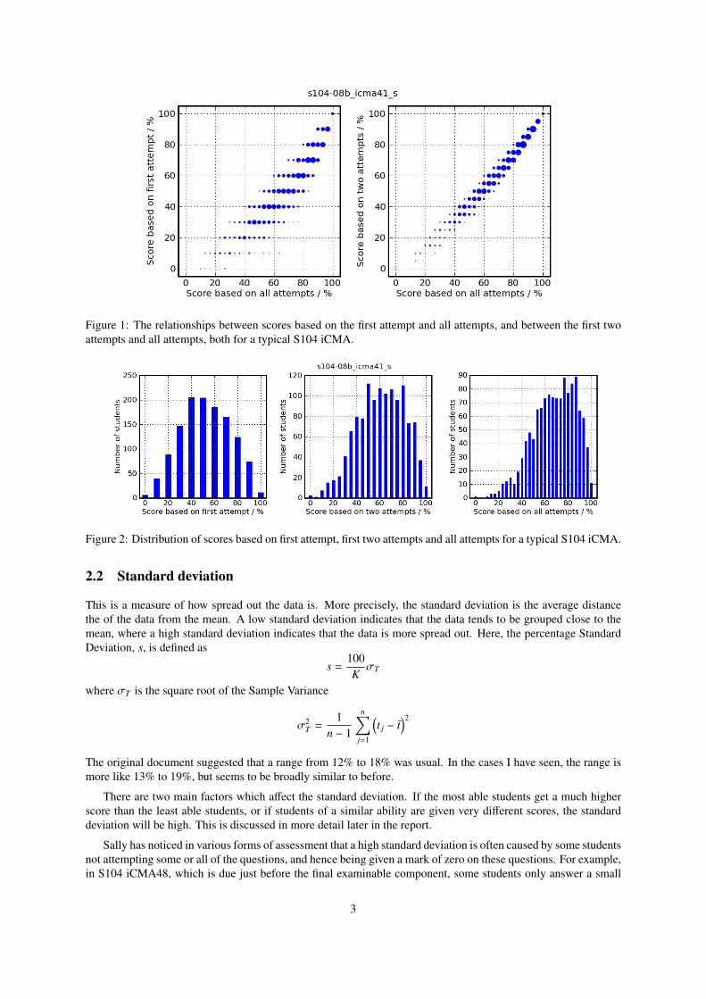
Figure 1: The relationships between scores based on the first attempt and all attempts, and between the first twoattempts and all attempts, both for a typical S104 iCMA.

Figure 2: Distribution of scores based on first attempt, first two attempts and all attempts for a typical S104 iCMA.

2.2 Standard deviation

This is a measure of how spread out the data is. More precisely, the standard deviation is the average distancethe of the data from the mean. A low standard deviation indicates that the data tends to be grouped close to themean, where a high standard deviation indicates that the data is more spread out. Here, the percentage StandardDeviation, s, is defined as

s =100KσT

where σT is the square root of the Sample Variance

σ2T =

1n − 1

n∑j=1

(t j − t̄

)2

The original document suggested that a range from 12% to 18% was usual. In the cases I have seen, the range ismore like 13% to 19%, but seems to be broadly similar to before.

There are two main factors which affect the standard deviation. If the most able students get a much higherscore than the least able students, or if students of a similar ability are given very different scores, the standarddeviation will be high. This is discussed in more detail later in the report.

Sally has noticed in various forms of assessment that a high standard deviation is often caused by some studentsnot attempting some or all of the questions, and hence being given a mark of zero on these questions. For example,in S104 iCMA48, which is due just before the final examinable component, some students only answer a small

3

Figure 3: The relationships between scores based on the first attempt and all attempts, and between the first twoattempts and all attempts, for an iCMA with 25 questions.

Figure 4: Skewness

number of questions and as a result the iCMA has a standard deviation of 24.4, significantly higher than mostother S104 iCMAs.

2.3 Skewness and Kurtosis

These measures are intended to describe the shape of the distribution of the total scores. Skewness is a measure ofthe asymmetry of the distribution. A negative skew generally indicates that most of the data is concentrated to theleft of the mean value, and a positive skew indicates that most of the data is to the right of the mean value. Typicalpositive and negative skewed distributions are shown in Figure 4.

Kurtosis is a measure of how peaked the distribution is. A distribution with positive kurtosis has a sharperpeak than the normal distribution, and has more points in the tails (so has a higher probability of extreme events).A distribution with negative kurtosis has a wider peak than the normal distributions, and has fewer points in thetails. Typical distributions with positive and negative kurtosis are shown in Figure 5 on the next page.

The use of these measures seems to be fairly limited. They are both used in tests to determine whether dataseems to be normally distributed, but here we already know that the overall scores are not normally distributed.The original document suggested that −1 was a typical value for Skewness, and 0 to 1 a typical value for Kurtosis.It is common for each value to be either substantially higher or lower than was suggested. It is not clear to mewhat useful inference about a test may be drawn from the skewness or kurtosis which might not be easier seen bylooking at the histogram of scores (see Section 2.5)

4

Figure 5: Kurtosis

2.4 Coefficient of Internal Consistency, Error Ratio, and Standard Error

Any one of these values, together with the Standard Deviation, can be used to calculate the other two, so theyessentially give us the same information. They are designed to tell us approximately how much of the variation ina student’s score is due to random effects and how much is due to how good the student is.

The Standard Error is intended to be an estimate of what the Standard Deviation would be if there was novariation between students. To calculate this under the new scheme, I worked out what the variance of the meanscore would be if the students all had the same probability as each other of scoring 0, 1, 2 or 3 on any givenquestion. The square root of this number then gives the Standard Error. I used the proportion of responses to eachquestion marked 0, 1, 2 or 3 as the probability (equal for each student) to get that score on that question, thenused probabilistic methods to calculate the standard deviation of the total score under this hypothesis. For furtherdetails of my calculations, see the end of the report.

My results are nearly identical to those found using a modified version of the original IET definition. Supposewe have I questions, then the original definition of Coefficient of Internal Consistency (used to calculate theStandard Error) contains a factor of I

I−1 , which I see no reason to include (see Section 5.1 on page 13). Removingthis factor gives a simple definition of the Standard Error:

Let Vi denote the variance of the ith question, ti j the jth student’s score and t̄i the average score on this question.Suppose that there are I questions in total. Then the Standard Error is

Standard Error =

√√√ I∑i=1

Vi

where

Vi =1

n − 1

n∑j=1

(ti j − t̄i

)2

I would recommend using this new definition of Standard Error instead of the existing definition. I would recom-mend alerting course teams if this Standard Error is greater than 12.

The Error Ratio expresses the Standard Error as a percentage of the Standard Deviation, and the Coefficientof Internal Consistency expresses the proportion of the variance which is not explained by chance effects alone.Instead of using at these proportions, I would recommend looking at the Standard Error, and also at what I willcall the “Systematic” Standard Deviation, which measures how much variation there is between students’ overalltest marks due to real differences in their ability:

Systematic Standard Deviation =

√σ2

T − (Standard Error)2

If the Standard Error is too high, then we expect students of a similar ability to get significantly different marksin the test, so students will have a high change of being given a mark too high or low. If the Systematic StandardDeviation is too low, then the test does not discriminate well between students of different abilities.

5

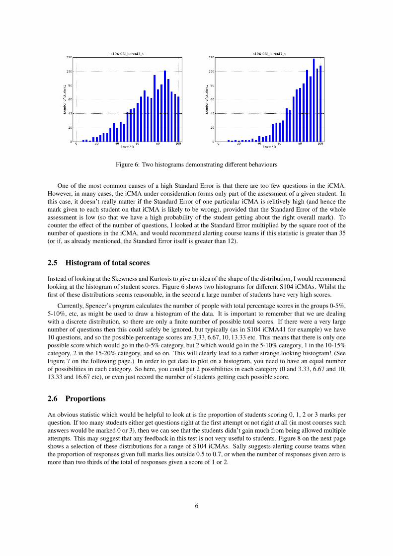
Figure 6: Two histograms demonstrating different behaviours

One of the most common causes of a high Standard Error is that there are too few questions in the iCMA.However, in many cases, the iCMA under consideration forms only part of the assessment of a given student. Inthis case, it doesn’t really matter if the Standard Error of one particular iCMA is relitively high (and hence themark given to each student on that iCMA is likely to be wrong), provided that the Standard Error of the wholeassessment is low (so that we have a high probability of the student getting about the right overall mark). Tocounter the effect of the number of questions, I looked at the Standard Error multiplied by the square root of thenumber of questions in the iCMA, and would recommend alerting course teams if this statistic is greater than 35(or if, as already mentioned, the Standard Error itself is greater than 12).

2.5 Histogram of total scores

Instead of looking at the Skewness and Kurtosis to give an idea of the shape of the distribution, I would recommendlooking at the histogram of student scores. Figure 6 shows two histograms for different S104 iCMAs. Whilst thefirst of these distributions seems reasonable, in the second a large number of students have very high scores.

Currently, Spencer’s program calculates the number of people with total percentage scores in the groups 0-5%,5-10%, etc, as might be used to draw a histogram of the data. It is important to remember that we are dealingwith a discrete distribution, so there are only a finite number of possible total scores. If there were a very largenumber of questions then this could safely be ignored, but typically (as in S104 iCMA41 for example) we have10 questions, and so the possible percentage scores are 3.33, 6.67, 10, 13.33 etc. This means that there is only onepossible score which would go in the 0-5% category, but 2 which would go in the 5-10% category, 1 in the 10-15%category, 2 in the 15-20% category, and so on. This will clearly lead to a rather strange looking histogram! (SeeFigure 7 on the following page.) In order to get data to plot on a histogram, you need to have an equal numberof possibilities in each category. So here, you could put 2 possibilities in each category (0 and 3.33, 6.67 and 10,13.33 and 16.67 etc), or even just record the number of students getting each possible score.

2.6 Proportions

An obvious statistic which would be helpful to look at is the proportion of students scoring 0, 1, 2 or 3 marks perquestion. If too many students either get questions right at the first attempt or not right at all (in most courses suchanswers would be marked 0 or 3), then we can see that the students didn’t gain much from being allowed multipleattempts. This may suggest that any feedback in this test is not very useful to students. Figure 8 on the next pageshows a selection of these distributions for a range of S104 iCMAs. Sally suggests alerting course teams whenthe proportion of responses given full marks lies outside 0.5 to 0.7, or when the number of responses given zero ismore than two thirds of the total of responses given a score of 1 or 2.

6

Figure 7: In some (common) circumstances, a histogram of scores with 5% cells can give misleading results.Sometimes it is better to plot a bar chart with a bar for each possible score.

Figure 8: The proportions of students who score 0, 1, 2 or 3 marks per question for several S104 iCMAs.

7

2.7 Can we recalculate the statistics based on first attempts only?

I have recalculated the statistics based on first attempts only, and compared the values to those suggested in the“Guide to CFAS Item Analysis”. Since the original statistics were designed for use with single attempt questions,they should be able to be applied in this case. However, it is not reasonable to expect that statistics calculatedbased on first attempts only and those calculated using data on all attempts will both fall into the same acceptableranges. For example, the mean score will be lower when only those who get the question right on the first go aregiven any credit. Since these questions were designed for use with multiple attempts, the mean score for the fulldata should fall within the range given by IET, not the first attempt score.

3 Interpretation of Question Statistics

These are the statistics designed to evaluate the performance of each question within a test.

3.1 Facility Index

Despite the impressive name, this is simply the average (mean) score on the question, expressed as a percentage ofthe maximum possible score on that question (defined similarly to the percentage mean score of the whole test).It gives an indication of how difficult the question is. A scale for interpreting the Facility Index is given in the“Guide to CFAS Item Analysis”. Very few questions are deterimined by this scale to be harder than “About rightfor average student” (That is, very few have Facility Index < 35%). A fairly large number of questions are markedas “Easy” (have Facility Index between 80% and 90%), or “Very Easy” (between 90% and 95%). It is likely thatthe scale needs some alterations, but it appears that some questions are genuinely too easy. Calculating the FacilityIndex (and other question statistics) based on all three attempts as opposed to just one will have a similar effect tothat described above for whole test statistics.

3.2 Standard Deviation

This is the percentage standard deviation for the question (defined similarly to the percentage standard deviation ofthe whole test). As for the whole test statistic, it shows how spread out the students’ scores are about the mean forthis question. The “Guide to CFAS Item Analysis” states that a standard deviation of less that 33% is not generallysatisfactory, presumably because a question with a low standard deviation would not be effective in discriminatingbetween students. A fairly large number of questions have standard deviation of less than this threshold, and asignificant number have standard deviation less than 20%.

3.3 Intended and Effective Weight

The intended weight is the maximum mark it is possible to score on a question. The effective weight is supposedto show how much the question actually contributes the the spread of scores. Its definition is a little dubiousbecause there is a remote possibility that it will involve taking the square root of a negative number. The EffectiveContribution to Variance, which is mentioned in “Guide to CFAS Item Analysis”, is a better defined quantity:the proportion of the variance which would be lost if question i was removed. However, it is perhaps less intu-itively straightforward than Effective Weight for non-expert users to interpret. I have now calculated the EffectiveContribution to Variance, and also the ratios of Effective Weight to Intended Weight and Effective Contribution toVariance to Intended Contribution to Variance. These ratios are useful measures, since they allow direct compari-son between questions with different Intended Weights or Intended Contribution to Variance.

3.4 Discrimination Index and Discrimination Efficiency

The Discrimination Index shows how well correlated the student’s scores on each question are with their scoreson the rest of the test. It ranges between −100 and 100, though a question with a negative Discrimination Index

8

Figure 9: The proportion of responses marked 0, 1, 2, or 3 for four questions in S104 iCMA41

would be rather strange, since it would indicate that students who scored low marks on this question scored highmarks on rest of the test, and vice versa. The larger the value of Discrimination Index, the better this question isas a predicator of how the student will do on the rest of the test.

At first sight, it may seem that the higher the Discrimination Index, the better. Indeed, questions with a highDiscrimination Index will tend to substantially lower the Standard Error for the iCMA or raise the SystematicStandard Deviation, which has to be a good thing. But if we consider the extreme case where all the questions arethe same, we would expect all questions to have a Discrimination Index very close to 100, but we might just aswell have had only one question on the test. Likewise, if we had a test where all but one question was the same,then the different question would probably have a low discrimination index.

Obviously, in real iCMAs students do not get asked the same question multiple times. But it is possible thatthe iCMA tests two parts of a student’s understanding. To understand this, suppose that a test had two types ofquestions: type A and type B, and that we had two types of students: α (who do well at type A questions) and β(who do well at type B). Then if we had lots of A questions, and very few B questions, then the A questions wouldhave a high Discrimination Index and the B questions a low Discrimination Index. This doesn’t mean that there isanything wrong with the B questions - maybe we just need more of them!

According to the “Guide to CFAS Item Analysis”, the Discrimination Efficiency is designed to stop questionswith a high mean being given a low Discrimination Index. I do not think it is a particularly useful measure, sincequestions which all students perform well at will not be good predictors of performance on the rest of the test (totake an extreme case: a question which all students got right would be useless)

3.5 Proportions

Again, it may be helpful to look at is the proportion of responses to each question which have been marked 0, 1, 2or 3. As Figure 9 shows, the behaviour can be quite extreme, even in questions which appear to be behaving wellaccording to other measures. Sally would recommend alerting course teams if the proportion of students scoring0 exceeds the combined proportion of students scoring 1 or 2.

3.6 Question Types

I was asked to consider these statistics for different types of questions: Multiple Choice, Multiple Response, Dragand Drop and similar questions, and then for the broader classes including numerical, text and free text questions.Everything as described above is valid for all these types of questions: provided that each student on each questionwill be given a score of 0, 1, 2 or 3.

However, there are some differences between the values the statistics take between different classes. Forexample, text and free text questions seem to have high proportions of students getting the question right at firstattempt, whearas numerical questions have a larger than average proportion of students not getting the questionright at all, as can be seen in Figures 10 to 12 on the next page.

9

Figure 10: The proportions of students who score 0, 1, 2 or 3 marks per question for multiple choice type questionsin S104.

Figure 11: The proportions of students who score 0, 1, 2 or 3 marks per question for questions in S104 requiringa numerical type answer.

Figure 12: The proportions of students who score 0, 1, 2 or 3 marks per question for questions in S104 requiringa text or free text answer.

10

4 Differences between variants

All variants are equal, but some variants are more equal than others

Often, students will not always be asked exactly the same question, but one “variant” of it. The purpose ofthis section of the report is to examine methods for determining whether or not all variants are the same difficulty,or more precisely, if a new student given the question would have an equal probability of scoring 0, 1, 2 or 3whichever variant he or she was given. If the variants are shown to be different, it would also be useful to seewhich groups of variants differed from which others, and to examine the nature of that difference.

Spencer’s program calculates the various question statistics separately for each variant. On some questions,the facility index differs greatly between variants, and so it seems intuitive that the variants are not all equallyhard. However:

1. it is difficult to guess how large the difference between facility indices would be if all variants were equallyhard, due to random differences in ability between students being asked each variant. Obviously you couldbe more sure that a certain spread of facility indices implied there was a real difference between variantsif there was a large number of students answering each variant, but it would be useful to have a precisemeasure to tell us if there was a statistically significant difference between variants.

2. it is possible for two variants to have similar facility indices and yet have very different spreads of scores.In S104 O8J iCMA48, questions 3 and 5 both have a difference of about 12% between the highest scoringvariant and the lowest scoring variant, have the same number of variants and a similar number of studentsattempting each variant. However, I plotted the proportion of students scoring 0, 1, 2 or 3 on each variant inboth of these questions, and the results (shown in Figure 13) look very different.

0.15

0.20

0.25

0.30

0.35

Interaction: score v. variant

score

mea

n of

pro

p

0 1 2 3

variant

250143

0.1

0.2

0.3

0.4

0.5

Interaction: score v. variant

score

mea

n of

pro

p

0 1 2 3

variant

435210

Figure 13: The proportions of students students scoring 0, 1, 2 or 3 on each variant in S104 O8J iCMA48 questions3 and 5, with p-values of 0.04 and 0.46 respectively

It would be useful to have a single figure which allows us to say with some certainty whether or not there is areal difference between variants. To do this, take the null hypothesis to be that all the probability of scoring 0, 1,2 or 3 is fixed across variants, and the alternative hypothesis that this is not the case.

Suppose there are J variants (J > 1), and let p0, p1, p2 and p3 be the overall proportions of students scoring0, 1, 2 or 3 on the question. Suppose there are n j students who got variant j. Then let oi j be the observed (actual)number of students scoring i on variant j, and ei j = n j pi be the the number of students you would expect to scorei on variant j if the null hypothesis was true. Define

D =

3∑i=0

J∑j=1

oi j lnoi j

ei j

11

0.0

0.2

0.4

0.6

0.8

Interaction: score v. variant

score

mea

n of

pro

p

0 1 2 3

variant

354012

0.1

0.2

0.3

0.4

0.5

0.6

0.7

Interaction: score v. variant

score

mea

n of

pro

p

0 1 2 3

variant

2103

0.15

0.20

0.25

0.30

0.35

Interaction: score v. variant

score

mea

n of

pro

p

0 1 2 3

variant

74610523

Figure 14: The behaviour of different variants of three S104 iCMA questions, with p-values of 0.53, 0, and 0.85respectively

Define p = Prob (X > D), where X ∼ χ2J+3. p is the probability that, under the null hypothesis that all variants

are equal, the numbers of students achieving each score under each variant would be at least as extreme as in theactual data. If p < 0.05, then you should reject the null hypothesis.

Going back to the example of S104 O8J iCMA48, questions 3 has p = 0.04 (so we reject the null hypothesis),and question 5 has p = 0.46 (so we accept the null hypothesis). This is in agreement with what can be seen fromFigure 13 on the previous page. In general, if you reject the null hypothesis, it is helpful to consider plots of theproportion of students scoring 0, 1, 2 or 3 on each variant in order to see which variants are causing the problem.Some more examples are shown in Figure 14. In S104 08J iCMA 41 question 4, it might seem from the plot (thethird in Figure 14) that there is a difference between variants, but in this case p = 0.85, so there is no statisticalreason to suppose that there is. This highlights that it is essential to use the plots carefully, and in conjunction withthe p-values.

12

5 Notes and Calculations

This section is not intended to be read as part of this report, rather to enable someone else to follow my reasoningin the future. It uses standard mathematical notation and requires a reasonable familiarity with probability.

5.1 Coefficient of Internal Consistency

Coefficient of Internal Consistency was originally defined as:

100 ×I

I − 1

1 − ∑Ii=1 Vi

σ2T

I think that the factor of I

I−1 should be removed. 1n−1

∑ni=1 (xi − x̄)2 is often used as an estimator of the population

variance from a sample of size n from that population (to give an unbiased estimator). Here we have I questionsin the whole population, and we calculate the variance Vi of each of them, and use each student’s total score overall I questions to give the total test variance σ2

T . We are using the whole population rather than a sample from it,and so the factor of I

I−1 is not necessary.

5.2 Standard Error

The Standard Error is intended to be an estimate of what the Standard Deviation would be if there was no variationbetween students. To calculate this, I worked out what the variance of the mean score would be if the students allhad fixed probabilities pi0, pi1, pi2 and pi3 of scoring 0, 1, 2 and 3 on question i. In my calculations I took theseprobabilities to be equal to the proportions of students scoring each mark on the question.

Now suppose we have n new students taking the test, all independent and with fixed probabilities of scoring 0,1, 2 or 3 on question i. Let Xi = (X0i, X1i, X2i, X3i) be the total number of students scoring 0, 1, 2 or 3 on questioni.

Then Xi, i = 1, . . . I are independent random vectors

Xi ∼ Multinomial (n; pi0, pi1, pi2, pi3)

So, letting Ti be the total score on question i:

Var (Ti) = Var (X1i + 2X2i + 3X3i)

= Var (X1i) + 4Var (X2i) + 9Var (X3i) + 4Cov (X1i, X2i) + 6Cov (X1i, X3i) + 12Cov (X2i, X3i)

= n[pi1(1 − pi1) + 4pi2(1 − pi2) + 9pi3(1 − pi3) − 4pi1 pi2 − 6pi1 pi3 − 4pi2 pi3

]The variance of the total score T is the sum of these question variances, so the variance of the average total score(T/n) is 1

n2

∑Ii=1 Var (Ti)

13