ICESat waveform-based land-cover classification using a curvematching approach

Yuhong Zhoua, Fang Qiua,b*, Ali A. Al-Dosaric, and Mohammed S. Alfarhand

aDepartment of Geospatial Science, University of Texas at Dallas, Richardson, TX 75080-3021,USA; bCentre of Geospatial Information, Shenzhen Institutes of Advanced Technology, Chinese

Academy of Sciences, Shenzhen, China; cDepartment of Geography, King Saud University, Riyadh11451, Saudi Arabia; dSpace Research Institute, King Abdulaziz City for Sciences and Technology,

Riyadh 11442, Saudi Arabia

(Received 12 February 2014; accepted 7 November 2014)

Light detection and ranging waveforms record the entire one-dimensional backscat-tered signal as a function of time within a footprint, which can potentially reflect thevertical structure information of the above-ground objects. This study aimed to explorethe potential of the Geoscience Laser Altimeter System sensor on board the Ice, Cloud,and Land Elevation Satellite to perform land-cover classification by using only theprofile curve of the full waveform. For this purpose, a curve matching method basedon Kolmogorov–Smirnov (KS) distance was developed to measure the curve similaritybetween an unknown waveform and a reference waveform. A set of reference wave-forms were first extracted from the training data set based on a principal componentanalysis (PCA). The unknown waveform was then compared with individual referencewaveforms derived using KS distance and assigned to the class with the closestsimilarity. The results demonstrated that the KS distance-based land-cover classifica-tion using the waveform curve was able to achieve an overall accuracy of 87.2% and akappa coefficient of 0.80. It outperformed the widely adopted rule-based method usingGaussian decomposition parameters by 3.5%. The research also indicated that thePCA- selected reference waveforms achieved substantially better results than randomlyselected reference waveforms.

1. Introduction

Land cover refers to the types of observed biophysical features covering the earth’s surface,such as water, trees, grass, roads, buildings, and bare ground. Land cover is increasinglyinfluenced and altered by human activities, causing it to constantly change over time. Theseland-cover changes can impose great pressure on the environment leading to widespreadproblems such as soil nutrient depletion (Abbasi, Zafar, and Khan 2007), landslides(Abbasi, Zafar, and Khan 2007), and global warming (Dallmeyer and Claussen 2011).Consequently, land cover has been monitored and assessed by geographers, ecologists, andother scientists in order to understand the ongoing processes driving its change and identifystrategies to achieve sustainable development.

A variety of data sources and methods have been utilized to derive land-coverinformation (Grey, Luckman, and Holland 2003). The traditional field survey approachis costly in terms of time and labour, inhibited by limited accessibility to many areasof land, and highly dependent on subjective human evaluation (Wu and Xing

*Corresponding author. Email: ffqiu@utdallas.edu

International Journal of Remote Sensing, 2015Vol. 36, No. 1, 36–60, http://dx.doi.org/10.1080/01431161.2014.990648

© 2014 Taylor & Francis

Dow

nloa

ded

by [

The

Uni

vers

ity o

f T

exas

at D

alla

s] a

t 14:

40 2

6 Ja

nuar

y 20

15

2010; Peerbhay, Mutanga, and Ismail 2013). Remote-sensing imagery, including multi-spectral, hyperspectral, and light detection and ranging (lidar) data, provides aneffective alternative to a field survey because of its ability to efficiently gather digitaldata from vast and inaccessible areas on a regular, repetitive basis (Arroyo et al.2010). Traditionally, remote sensing of land cover primarily relied on multispectralimagery (e.g. Landsat Thematic Mapper and Systeme Probatoire d’Observation de laTerre) (Jawak and Luis 2013). Its use for general land-cover classification has beenwidely studied (Harvey and Hill 2001; Li, Ustin, and Lay 2005), but poor spectralresolution because of a limited number of bands and wide bandwidths inhibits detailedland-cover classification, especially discriminating different geographical features thathave similar spectral responses (Rosso, Ustin, and Hastings 2005). The spectraldifferences among different types of land cover may occur in very narrow regionsof the spectrum that cannot be sensed by multispectral sensors. The advent ofhyperspectral data offers a promising alternative for performing land-cover classifica-tion at a much more detailed level. The subtle spectral differences among differentmaterials can be sensed by the hundreds of contiguous narrow bands (often 10 nm orless) of the hyperspectral data (Cho et al. 2010) allowing, for example, the discrimina-tion of tree species or differentiation of mineral types. However, both multispectraland hyperspectral data can only provide spectral information of an object’s surface andmay fail to separate objects that are spectrally similar but structurally different(Buddenbaum, Seeling, and Hill 2013). For example, roads and buildings are spec-trally similar when they are constructed using the same material (such as concrete).Differentiation may be difficult, even with hyperspectral data.

Unlike multispectral and hyperspectral remote sensing, the recently available lidartechnology can potentially provide structural information about an object through thethree-dimensional positional measurements recorded by its return pulse (Sasaki et al.2012). Lidar is an active remote-sensing technology based on ranging using visible,near-infrared, or short-wave infrared laser beams. Lidar data can be divided into twocategories based on how the signal is recorded: discrete-return lidar and full-waveformlidar (Alexander et al. 2010). For discrete-return lidar, the continuous reflection signalis discretized into one or multiple returns. Conversely, full-waveform lidar records theentire backscattered signal of the objects along the path of the emitted laser usingsmall time intervals (typically 1 ns) which determine the level of vertical detail (Faridet al. 2008; Zaletnyik, Laky, and Toth 2010; Pirotti 2010; Mallet et al. 2011). Toperform land-cover classification, discrete-return lidar data are used independently orin conjunction with multispectral or hyperspectral data. For example, Vögtle andSteinle (2003) used lidar elevation data alone to classify urban features into trees,buildings, and terrain objects, achieving an overall accuracy of 91%. Although thediscrimination between objects with distinct vertical structures is high, the ability ofdiscrete-return lidar to separate objects with no vertical structure (e.g. bare land andgrass) or similar vertical structures is limited. Consequently, numerous subsequentstudies have integrated imagery data (either multispectral or hyperspectral) and dis-crete-return lidar data to improve classification performance (Sugumaran and Voss2007; Zhou and Troy 2008; Sasaki et al. 2012).

Full-waveform lidar, which has become operational only recently, provides apromising new source to monitor land-cover conditions. The shape of a waveform isthe result of interaction between the transmitted laser pulse and intercepted objectsurfaces within the lidar footprint (Alexander et al. 2010; Pirotti 2010). For example, awaveform over a building is primarily determined by the joint effects of the building’s

International Journal of Remote Sensing 37

Dow

nloa

ded

by [

The

Uni

vers

ity o

f T

exas

at D

alla

s] a

t 14:

40 2

6 Ja

nuar

y 20

15

height, vertical structure, and the percentage of area covered by ground versus build-ing within the footprint. A waveform over a tree is often determined by tree density,structure, and vegetation phase. Due to the finer vertical resolution, a lidar waveformoffers an enhanced capability to reflect the vertical structures of geographical objectscompared to the traditional discrete-return lidar that typically consists of six or fewermeasurements separated by several metres in distance along its vertical profile(Zaletnyik, Laky, and Toth 2010; Zhang et al. 2011; Ussyshkin and Theriault 2011).The large-footprint waveform data collected by the Geoscience Laser AltimeterSystem (GLAS) on board the Ice, Cloud, and Land Elevation Satellite (ICESat) isthe most commonly used due to its availability free-of-charge, global coverage, andrepeatable measurements (Ranson et al. 2004; Duong, Pfeifer, and Lindenbergh 2006;Pirotti 2010; Wu and Xing 2010; Zhang et al. 2011; Molijn, Lindenbergh, and Gunter2011). Although originally designed for cryosphere research, ICESat waveforms havebeen widely used for various other studies, such as estimation of above-groundbiomass (Lefsky et al. 2005; Ballhorn, Jubanski, and Siegert 2011; Boudreau et al.2008; Duncanson, Niemann, and Wulder 2010; Nelson 2010), canopy vertical struc-ture (Harding and Carabajal 2005; Lee et al. 2011; Sun et al. 2008; Duncanson,Niemann, and Wulder 2010; Lefsky et al. 2007; Pang et al. 2011; Rosette, North,and Suárez 2008; Wang et al. 2012, 2014), timber volume (Nelson et al. 2009; Ransonet al. 2007), and building height (Gong et al. 2011).

ICESat waveforms have also been used for land-cover classification by a number ofresearchers (Ranson et al. 2004; Duong, Pfeifer, and Lindenbergh 2006; Zhang et al.2011; Wu and Xing 2010; Molijn, Lindenbergh, and Gunter 2011; Wang et al. 2012; Liuet al. 2014), since a waveform shape is largely determined by the vertical structures of theobjects within the footprint. In general, the waveform shape is composed of one or manyechoes, where one echo is a peak in the waveform that may correspond to an individualtarget encountered or a cluster of objects too close to be separated, while multiple echoesoften represent multiple targets or one target with multiple components that are verticallyseparable within the footprint (Alexander et al. 2010). Consequently, the shapes for thewaveforms over multiple objects can be very complex. To utilize the waveforms for land-cover classification, existing studies have focused on simplifying the complex full-wave-form data. Shape-related summary metrics derived from the full waveform, such as thenumber of echoes, peak amplitude, echo width, skewness, and kurtosis, are used torepresent the important characteristics of the waveform shapes (Ranson et al. 2004;Duong, Pfeifer, and Lindenbergh 2006; Zhang et al. 2011; Narayanan, Kim, and Sohn2009; Zaletnyik, Laky, and Toth 2010; Wu and Xing 2010; Molijn, Lindenbergh, andGunter 2011; Mallet et al. 2011; Wang et al. 2012). These metrics have had varied successin differentiating land-cover types. Because they aim to reduce the complexity of thewaveform data, these metrics are not taking advantage of the entirety of information thatthe full waveform offers. The full-waveform curve provides a more comprehensive pictureof the vertical structure of the intercepted surfaces than these summary metrics. Thisvertical structure information is potentially more valuable for land-cover classification byusing a curve-matching-based approach, but has been scarcely investigated.

To complement the research based on summary metrics of the full waveforms, thisstudy focuses on analysing the complete curve distribution. It investigates a novelapproach derived from the Kolmogorov–Smirnov (KS) statistic (Burt and Barber1996) for analysing the full ICESat waveform to distinguish land-cover types. Thespecific objectives of the study are (1) to quantify the similarity between waveformcurves using a KS-based approach; (2) to select a set of waveforms as references

38 Y. Zhou et al.

Dow

nloa

ded

by [

The

Uni

vers

ity o

f T

exas

at D

alla

s] a

t 14:

40 2

6 Ja

nuar

y 20

15

through principal component analysis (PCA); and (3) to determine whether analysingthe complete curve distribution using the KS-based approach can achieve superiorresults for land-cover classification over a rule-based approach using Gaussian decom-posed parameters.

In this study, the emphasis is on exploring the potential of full waveforms alone todifferentiate objects having different vertical structures using a curve-matching-basedapproach. Consequently, spectral information was deliberately excluded, and a relativelylevel study area was used to minimize the complications of a varied terrain. Furthermore,only three general categories of land cover that have distinct vertical structures are used:buildings, trees, and open spaces. All land-cover types with a flat open surface such asbare land, water, roads, and parking lots are assigned to the open space category. They arenot identified as separate categories since they have generally similar vertical waveformcurves and it is very difficult to classify them using the waveform lidar alone. Similarly,there is no differentiation of building subtypes (such as residential or commercial) or treesubtypes (such as deciduous or coniferous). These very general land-cover categorieswere a necessity following from the use of ICESat waveform data, which do not allow amore detailed level of classification because of the large size of the ICESat footprint(Hilbert and Schmullius 2012). Albeit not optimal for land-cover classification since itwas designed for other purposes, the free availability of its waveforms makes it anespecially useful test bed for assessing curve-matching-based approaches. Furthermore,global coverage is available since it is a satellite-based system. If the effectiveness ofusing full-waveform curves alone for high-level land-cover classification can be achieved,future studies can then be conducted by incorporating spectral information of high spatialresolution (HSR) imagery with small-footprint waveform curves from commercial air-borne lidar systems at the object level to achieve a more detailed land-cover classificationor fusing hyperspectral imagery with pseudo-waveforms derived from discrete-return lidarto identify vegetation species using the same curve matching approach.

2. Study area and data

2.1. Study area

The study area is located in the Dallas, Texas metropolitan area, bounded approximatelyby 97.031° to 96.518° W and 32.553° to 32.996° N, where a large number of ICESatwaveform data are available (Figure 1). The area is characterized by a mixture of matureresidential neighbourhoods and commercial and industrial buildings.

ICESat waveforms are sensitive to surface terrain due to their large footprints (Hilbertand Schmullius 2012). For example, a waveform over open space with a flat surface(Figure 2(a)) usually presents a single echo with a narrow width because a high concen-tration of energy is reflected back at nearly the same time, while a waveform over openspace with a sloped surface (Figure 2(b), not in our study area but was selected from ahilly area of San Diego) is stretched with multiple echoes due to rough terrain topography.The waveform widths can be noticeably wider compared to those of flat surface if terrainslopes are larger than 10° (Hilbert and Schmullius 2012). Since the majority of the studyarea is composed of flat surfaces (slope ≤ 10°), the terrain is not expected to exertsignificant influence on the waveform shapes (Gong et al. 2011; Hilbert and Schmullius2012; Duong et al. 2009) and therefore the classification.

International Journal of Remote Sensing 39

Dow

nloa

ded

by [

The

Uni

vers

ity o

f T

exas

at D

alla

s] a

t 14:

40 2

6 Ja

nuar

y 20

15

Figure 1. Study area with waveform footprints.

0.08

0.04

0.01

00.

000

Ene

rgy

(V)

650 750

(a) (b)

850 950Time (ns)

650 750 850 950Time (ns)

Ene

rgy

(V)

0.00

Figure 2. (a) A waveform over open space with flat surface and (b) a waveform over open spacewith sloped surface.

40 Y. Zhou et al.

Dow

nloa

ded

by [

The

Uni

vers

ity o

f T

exas

at D

alla

s] a

t 14:

40 2

6 Ja

nuar

y 20

15

2.2. ICESat/GLAS full waveform

Up to now, ICESat is the only spaceborne laser satellite (Wu and Xing 2010), althoughairborne lidar systems are increasingly available with the capability of collecting medium-or small-footprint waveforms. One of the objectives for ICESat is to measure surfaceelevation and vegetation cover globally. It was launched by NASA in January 2003, cameinto operation about one month later, and operated at an orbit altitude of 600 km until itstermination in October 2009. There were 18 operational periods in total during this 7-yearmission, collecting about two billion waveforms (Nelson 2010). During most operationalyears, the ICESat was programmed with a 91-day repeat orbit (Sun et al. 2008). TheGLAS on board ICESat uses the near-infrared (~1064 nm) channel to acquire verticalprofiles of returned energy as a waveform with a frequency of 40 Hz (Pirotti 2010). Forthe beginning missions in 2003, the received waveforms over land have 544 bins thatcorrespond to an 81.6 m vertical extent with a 1 ns temporal interval. Starting from 2004,the vertical extent of the waveform was increased to 150 m in order to obtain returns fromtaller objects (>81.6 m). The returns lower than 58.8 m (lower 392 bins) have a 1 nsinterval and the returns higher than 58.8 m (upper 152 bins) have a 4 ns interval (Hardingand Carabajal 2005). This results in a total of 1000 ns to record reflected intensity ofICESat waveforms. The footprints are elliptical in shape and their sizes vary a great dealbetween different missions, with a mean major axis ranging from about 50 to 150 m(Attributes for ICESat Laser Operations Periods, 2009). The average spacing betweenadjacent footprints along the track is about 175 m.

The ICESat programme distributes 15 Level-1 and Level-2 data products (labelledGLA01 to GLA15), which are readily available on the National Snow & Ice Data Centerwebsite. For this study, we employed the Level-1A global altimetry data GLA01, whichincludes the raw waveform, Level-1B global waveform-based range correction dataGLA05, which contains parameters for the shape of footprints, and the Level-2 globalland surface altimetry product GLA14, which contains the centroid coordinates of thewaveform footprints. All GLA01, GLA05, and GLA14 contain the unique record indexnumber and shot number, which together can be used to link a waveform to its corre-sponding footprint. For the study area, the waveform data set was obtained for the entiretyof 2005 (including 17 February 2005, 23 May 2005, and 24 October 2005) and 2006 (25February 2006, 27 May 2006, and 27 October 2006), including 2183 waveforms.

2.3. Ground reference data

The National Land Cover Database 2006 (NLCD2006) was used to obtain groundreference data for each waveform. NLCD2006 is a 16-class land-cover classificationdata set that is consistently available across the conterminous United States with a spatialresolution of 30 m (Fry et al. 2011). In this study, the pixels of interest were thosepredominately occupied by buildings, trees, or open spaces. Google Earth images werefurther employed to refine the ground reference data for each selected ICESat footprint.Google Earth has been used as a reliable source of reference data for remote-sensing-based land-cover classification in recent years (Helmer, Lefsky, and Roberts 2009) as itprovides imagery with HSR. The availability of historical imagery in Google Earth since2001 allowed comparison with the 2005 and 2006 ICESat data. In order to minimize thetime difference between the ICESat waveform data and the land-cover ground referencedata, Google Earth reference images closest in time to the waveform data were used.

International Journal of Remote Sensing 41

Dow

nloa

ded

by [

The

Uni

vers

ity o

f T

exas

at D

alla

s] a

t 14:

40 2

6 Ja

nuar

y 20

15

The approximate areas of the waveform footprints were computed using the ellipsesdefined by their short and long axes, together with the orientations of the long axis,derived from the parameters provided in the GLA05 product (Gong et al. 2011). Thewaveform footprint polygons thus obtained were then converted to keyhole markuplanguage and imported to Google Earth. When these ICESat footprints are overlaid ontop of Google Earth images, the land-cover conditions within the selected footprints canthen be determined through visual interpretation.

Since the waveform shapes were primarily determined by the vertical structures of thedominant land-cover type within the footprints, only waveforms having a dominant land-cover type were identified for each class to investigate whether the vertical structureinformation provided the by lidar waveform can be better extracted by using a curve-matching-based method when compared to a rule-based method using Gaussian decom-posed parameters. This was relatively easy to achieve for the open space category due tocommon presence of large open spaces in Dallas. However, due to the likely presence ofbare land, grass with a mix of buildings, and trees inside the large ICESat footprints, onlywaveforms where buildings or trees covered more than 50% of the area of their footprintswere considered as buildings or trees, respectively. The waveform footprints that did nothave a dominant land-cover type but had a mixture of several dominant types were excludedfrom the training and testing processes because they cannot be easily labelled with a singleclass in a hard classification such as the ones used in this study. Like a mixed pixel, theclassification of mixed footprints should be investigated using a fuzzy classification algo-rithm in the future, which is not the focus of this study. If the potential of waveform curvesusing a curve-matching-based approach can be demonstrated, we will incorporate wave-form curves with HSR imagery at the object level for fine-scale land-cover classification.Since the footprints of these objects are derived from HSR imagery through image seg-mentation, the mixed footprint problem will not be an issue any more because each imagesegment usually has a dominant land-cover type as a result of segmentation.

3. Methodology

As discussed earlier, the land cover of the study area was classified into three categories:buildings, trees, and open spaces. The methodological steps required for this classificationare summarized in the flow chart in Figure 3. The waveform samples are initiallypreprocessed by transforming coordinates, excluding unreliable waveforms, and removingsystem noise. The whole data set is then equally split into training and testing parts byrandom sampling within each category. A set of reference waveforms is selected from thetraining data set by using a method based on a PCA. For the testing part, each waveformis assigned to the class of a reference waveform with the closest similarity. KS distance isused as a similarity measurement to match the unknown waveform with a referencewaveform of known land-cover type. To assess the performance of this KS distance-based land-cover classification approach, a widely used rule-based approach based onGaussian decomposed parameters is also implemented for comparison purposes. Finally,the accuracies of the classification results from the KS distance and rule-based approachesare evaluated. These steps are described in more detail later.

3.1. Preprocessing

Preprocessing was performed to make waveform data suitable for further analysis.First, both GLA01 and GLA14 were converted from distributed binary format (*.dat)

42 Y. Zhou et al.

Dow

nloa

ded

by [

The

Uni

vers

ity o

f T

exas

at D

alla

s] a

t 14:

40 2

6 Ja

nuar

y 20

15

to ASCII format and the unit of GLA01 was converted from count (0–255) to voltage.Then, the ellipsoid of GLA14 was transformed from the default TOPEX/Poseidon tothe WGS84 coordinate system, since other geographical data used the WGS system.Second, unreliable waveforms, such as those with a reflectivity (the i_reflctUncorrfield in GLA14) lower than 0.1 (Molijn, Lindenbergh, and Gunter 2011), a value ofi_satCorrFlg in GLA14 larger than 0 (Duong et al. 2009), or a signal-to-noise ratiolower than 10 (Hilbert and Schmullius 2012; Hayashi et al. 2013), were excludedbecause they were primarily caused by heavy cloud. As a result, 844 waveforms wereretained with 391, 270, and 183 waveforms for open space, tree, and buildingcategories, respectively. Lastly, a noise removal procedure was applied to eliminatesystem noise at the beginning and end of each waveform signal. Any waveform signal

Figure 3. General flow chart of methodology.

International Journal of Remote Sensing 43

Dow

nloa

ded

by [

The

Uni

vers

ity o

f T

exas

at D

alla

s] a

t 14:

40 2

6 Ja

nuar

y 20

15

value below the threshold was regarded as noise and assigned a value of 0. Thethreshold was determined using i 4nsBgMeanþ 4:5� i 4nsBgSDEV (Lefsky et al.2007), where i_4nsBgMean is the mean value of the background noise for the 4 nsfilter and i_4nsBgSDEV is the standard deviation of the background noise for the 4 nsfilter. Both were the variables in GLA01. The starting location of a waveform wasdefined by finding the furthest left location of the waveform where the signal waslarger than the threshold value, and the ending location was identified by the right-most location where the signal was larger than the threshold value (Figure 4). Amongall the reliable waveforms, the earliest starting location was the 651th ns (correspond-ing to the top of the highest object), and the last ending location was close to the1000th ns value (corresponding to the lowest ground level). Therefore, only signalsover the last 350 ns (from 651th to 1000th ns) were analysed in this study.

3.2. Kolmogorov–Smirnov distance based approach

3.2.1. Reference waveform selection

After preprocessing, the data set was randomly split into training and testing parts(Table 1). The number of training waveforms for buildings, trees, and open space was91, 135, and 195, respectively. In traditional land-cover classification based onstatistical methods such as maximum likelihood, all training data are used to estimatethe statistical parameters of the classification model, and subsequent classification isperformed based on the trained model without further reference to the original training

650

1.2

1.0

0.8

0.6

0.4

0.2

0.0

Ene

rgy

(V)

700 750

Amplitude

StartinglocationThreshold

Endinglocation

800 850Time (ns)

900 950 1000

Figure 4. Waveform characteristics.

Table 1. The number of training and testing waveform samples.

No. of training waveforms No. of testing waveforms No. of selected waveforms

Building 91 92 183Tree 135 135 270Open space 195 196 391Total 421 423 844

44 Y. Zhou et al.

Dow

nloa

ded

by [

The

Uni

vers

ity o

f T

exas

at D

alla

s] a

t 14:

40 2

6 Ja

nuar

y 20

15

samples. Since the KS distance is a curve matching approach that is based onmeasuring the similarity between an unknown sample and individual references, amethod is required to select a subset of references from the training samples. On theone hand, many waveforms for a given land-cover category have a similar profile inthe training data set. For example, most of the waveforms for open space have similarsingle-echo shapes, with minor differences in the starting and ending location, thewidth, or the peak amplitude of the echoes. Consequently, to avoid data redundancy, itis not appropriate to use all training samples in a land-cover category. On the otherhand, there also exist substantial differences between the waveform curves of the samecategory, a phenomenon often referred to within-class variability. Due to their differentheight levels and vertical structures, the waveform curves of the same land-covercategory in the training data set can be very different from each other, especially forbuildings and trees. Therefore, it is also important that the reference waveforms beable to adequately capture the within-class variability for each category. To resolve thedilemma of avoiding duplication while also reflecting variation, a multiple referencewaveform selection approach was developed, beginning with a PCA. PCA has thecapability to decorrelate the input data and remove duplication by maximizing thevariability on the principal components and selecting subsequent orthogonal compo-nents in descending order of variance (Sarrazin et al. 2012). Thus, the first principalcomponent should be able to reflect the main trend of waveform distributions and isused to select the first reference waveform in each land-cover category. Intuitively, weshould use the subsequent components to select other references. However, the curvesof the subsequent principal components are drastically different in shape from all thetraining waveforms in each category and so an alternative approach was used tocapture within-class variability.

For each land-cover category, each training waveform was assumed to be an inputvariable to the PCA, and each time bin (1 ns) of a waveform was assumed to be anobservation. For example, the open space category had 195 waveforms and eachwaveform had 350 bins of interest; thus, there were 195 input variables each with350 observations in the open space category. Although the original waveform curvescould be used, this study used their cumulative distribution functions (CDFs) as inputvariables to the PCA. This provides consistency with the KS approach which is basedon CDFs. Additionally, correlation coefficients between the CDFs are significantlyhigher compared to those for the original waveforms due to the monotonic growth ofCDFs. For example, the correlation coefficient between the original waveforms forbuilding in Figure 5(e) and building in Figure 5(g) is about 0.27, although theypresent similar patterns. The coefficient is increased to 0.92 when the CDF curvesare used.

The procedure for the PCA-based reference waveform selection was implemented asfollows.

Step 1: For each category, apply PCA to all the training waveforms and then find thetraining waveform with the best similarity to the first PCA component using the smallestKS distance (which is discussed later). Store it as the first reference waveform in thereference set since it is closest to the first component that explains the largest majority ofvariance in the data.

Step 2: Compute the KS distance between all other training waveforms and thefirst reference waveform. The training waveform with the smallest (least) similarity(that is, the largest KS distance) to the first reference is selected as the second

International Journal of Remote Sensing 45

Dow

nloa

ded

by [

The

Uni

vers

ity o

f T

exas

at D

alla

s] a

t 14:

40 2

6 Ja

nuar

y 20

15

reference waveform. This reference waveform is most different from the first referencewaveform within the same land-cover category.

Step 3: The next reference waveform to be selected is based on the smallest totalsimilarity (i.e. the largest total KS distance) between a training waveform and allcurrently selected reference waveforms. The reference set R now has two referencewaveforms, i.e. R ¼ R1;R2f g, and assume that the training set Q has n remainingsamples, i.e. Q ¼ Q1;Q2; . . .Qi . . .Qnf g. Calculate the KS distance between Qi and R1

and R2 as KSi1 and KSi2, respectively. Sum Ki1, KSi1, and KSi2 to obtain the total KSdistance TKSi. Sort all TKSi and the one with the largest total KS distance (i.e. thesmallest similarity) is selected as the next reference waveform.

Step 4: Repeat step 3 until the smallest total similarity between the trainingwaveform and existing reference waveforms is smaller than a given threshold.Multiple threshold values were tested, and threshold values of 0.20, 0.25, and 0.20for tree, building, and open space categories, respectively, were empirically found toproduce the most accurate classification results for the training data set.Theoretically, the extracted reference waveforms, although being a small subset ofthe original training samples, should represent most of the typical samples for eachcategory in the training data set. These selected reference waveforms are then usedto classify waveforms in the testing data set.

3.2.2. Kolmogorov–Smirnov distance

KS distance is often used to measure the similarity between two empirical frequencydistributions in the non-parametric KS statistical test (Burt and Barber 1996). The

650

(a)

(e)

(i) (j) (k) (l)

(f) (g) (h)

(b) (c) (d)1.

20.

8 0.8

0.4 0.4

0.0

1.2

0.8

0.4

0.0

0.0

Ene

rgy

(V)

0.8

0.4

0.0

0.00

0.15

0.30

Ene

rgy

(V)

Ene

rgy

(V)

0.8

0.4

0.0

0.8

0.4

0.0E

nerg

y (V

)E

nerg

y (V

)

1.2

0.8

0.4

0.0

Ene

rgy

(V)

CD

F

0.8

0.4

0.0

CD

F

0.8

0.4

0.0

CD

F

CD

F

0.8

0.4

0.0

CD

F

0.8

0.4

0.0

CD

F

750

Open space

Building

Tree Tree Tree Tree

Building Building Building

Open space Open space Open space

850 950

Time (ns)

650 750 850 950

Time (ns)

650 750 850 950

Time (ns)

650 750 850 950

Time (ns)

650 750 850 950

Time (ns)

650 750 850 950

Time (ns)

650 750 850 950

Time (ns)

650 750 850 950

Time (ns)

650 750 850 950

Time (ns)

650 750 850 950

Time (ns)

650 750 850 950

Time (ns)

650 750 850 950

Time (ns)

Figure 5. Pairwise typical original waveform and the corresponding CDF. (a), (c), (e), (g), (i), and(k) are original waveforms and (b), (d), (f), (h), (j), and (l) are their corresponding CDF, respectively.

46 Y. Zhou et al.

Dow

nloa

ded

by [

The

Uni

vers

ity o

f T

exas

at D

alla

s] a

t 14:

40 2

6 Ja

nuar

y 20

15

motivation to use KS distance to classify waveform data is inspired by our recentlydeveloped fuzzy KS classifier for land-cover classification using HSR data (Sridharanand Qiu 2013). In this classifier, the empirical cumulative distribution of spectral valueswithin each object is used to compare the object-to-object similarity. According toZhang et al. (2011) and Pirotti (2010), the ICESat waveforms of GLA01 were originallystored as the counts (0–255) of returning impulse along the time axis. Therefore, awaveform can be treated as a time-varying frequency distribution function (histogram)(Zaletnyik, Laky, and Toth 2010). Muss, Mladenoff, and Townsend (2011) employed aheight frequency distribution of discrete-return lidar points within a forest stand or a plotto simulate the corresponding pseudo-waveform using a cubic spline function. It wasdemonstrated that the resultant pseudo-waveform is similar in its characteristics to thetraditional waveform, since the height essentially corresponds to time multiplied by thespeed of light. For these reasons, the KS distance can be calculated based on either thetrue or pseudo-waveform to measure the similarity of their corresponding empiricalfrequency distributions.

Figure 5 shows that the CDFs of waveforms corresponding to different land-cover types are noticeably distinct from each other. Waveforms for open space oftenhave a single, narrow echo resulting in a steeply increasing edge in the correspond-ing CDFs, which quickly reaches one. A typical building waveform usually has twonarrow echoes, one for the building roof and the other for the ground, with a gapbetween them corresponding to the building height. This results in the steep stepsobserved in the CDF. As for trees, the waveforms usually have two major echoeswith varied width: a wider top echo corresponding to the tree crown and a narrowersecond echo corresponding to the ground. Accordingly, the CDF gradually increasesinitially with gentle slopes but the end reaches one abruptly when the signal hits theground.

Figure 5 also suggests that, compared with the original waveforms, the CDFs maybe able to reduce within-class variability. For example, due to the differences in thelocal ups and downs and in the global patterns such as the echo widths and peakamplitudes, the original waveforms for tree in Figure 5(i) and tree in Figure 5(k) havequite different shapes, but their corresponding CDFs are more similar to each other inshape because the local and global differences are minimized during the aggregation andnormalization process inherent in creating the CDFs. Therefore, the use of CDFs mayhelp reduce the omission error of the classification. On the other hand, the CDF curvesmay also increase the between-class similarity, because the similarity between the CDFsof different categories may become larger than that between their original waveforms forthe same reason, which may potentially increase the omission error. For example, theCDFs of open space in Figure 5(b) and building in Figure 5(f) are now a little moresimilar to each other compared to their original waveforms, but still with considerabledistinction, especially in the slope of the steps. The KS distance is not based on a point-by-point comparison of the two CDFs at every bin. It is the maximum differencebetween two CDF curves, which is actually the cumulative difference between thetwo. Therefore, KS distance can capture the major difference in the patterns of theCDFs, such as the slope of the steps.

Based on the two-sample KS distance, the following steps were employed to evaluatewhether the CDF of an unknown waveform is similar to that of a reference waveform.

Step 1: For all input waveforms, the CDF is first computed using Equation (1). Thisalso serves as a normalization process to make waveforms acquired in different epochs orwith different atmosphere conditions comparable with each other.

International Journal of Remote Sensing 47

Dow

nloa

ded

by [

The

Uni

vers

ity o

f T

exas

at D

alla

s] a

t 14:

40 2

6 Ja

nuar

y 20

15

S ið Þ ¼Pi

j¼min VjPmaxj¼min Vj

; (1)

where Vj is the received energy at the time jth ns. In this study, min equals 651 and maxequals 1000, because only the last 350 ns (from 651 ns to 1000 ns) are of interest.

Step 2: To assess similarity, KS distance is measured as the maximum absolutedistance between the CDF of an unknown waveform and that of each reference waveformusing Equation (2),

Dk ¼ MAXmin� i�max

Srk ið Þ � St ið Þ

�� ��; k ¼ 1; 2; � � � ;K; (2)

where Srk is the CDF of the kth reference waveform and St is the CDF of an unknown

waveform.Step 3: For classification, the unknown waveform is assigned to the reference class

with the smallest KS distance (Equation (3)).

k̂ ¼ arg min1� k�K

Dk : (3)

As an example, it is apparent in Figure 6 that the CDF of an unknown waveformclosely resembles that of the open space reference waveform, rather than the CDFsof the building and tree reference waveforms. The maximum absolute distance,measured vertically, between the CDF of this unknown waveform and that of theopen space reference waveform is therefore the minimum among all the Dk . As aresult, the unknown waveform is classified into the open space category.

3.3. Rule-based approach

Rule-based methods based on parameters extracted from preprocessed and Gaussiandecomposed waveforms have been widely adopted for land-cover classification(Duong, Pfeifer, and Lindenbergh 2006; Alexander et al. 2010). In this study, a

650

UnknownTreeOpen spaceBuilding

1.0

0.8

0.6

0.4

0.2

0.0

CD

F

700 750 800 850 900 950 1000Time (ns)

Figure 6. CDFs of three reference waveforms and an unknown waveform. The vertical black linesare the maximum absolute distances between the CDF of the unknown waveform and that of theindividual reference waveform.

48 Y. Zhou et al.

Dow

nloa

ded

by [

The

Uni

vers

ity o

f T

exas

at D

alla

s] a

t 14:

40 2

6 Ja

nuar

y 20

15

rule-based classification approach using ICESat waveforms was also implemented forcomparison with the KS-based approach. The first step of the rule-based approachinvolved preprocessing as described in Section 3.1 to extract the values of the startingand ending locations. The next step, Gaussian decomposition, assumes that waveformw tð Þ is a mixture of k Gaussian distribution components (echoes) Wj tð Þ. Thus, awaveform can be expressed as Equation (4),

w tð Þ ¼Xk

j¼1

Wj tð Þ;with Wj tð Þ ¼ Aje� t�μjð Þ2

2σj2: (4)

where w tð Þ is the received energy of the waveform at time t, k is the number ofGaussian components, Wj tð Þ is the contribution of the jth component at time t, Aj is theamplitude of component j, μj is the mean of component j, and σj is the standarddeviation of component j. An expectation-maximization (EM) algorithm (Oliver,Baxter, and Wallance 1996) is applied to decompose the waveform into a series ofGaussian components by estimating the values for k, Aj, μj, and σj. Figure 7 presents anoriginal waveform with multiple peaks, which is decomposed into three Gaussiancomponents by using the EM algorithm.

Preprocessing and Gaussian decomposition result in the following parameters foreach waveform: s.loc (starting location) and e.loc (ending location), width (the dis-tance between starting location and ending location of the noise-removed waveform), k(the number of Gaussian components), and Am (amplitude), μ (mean), and σ ðstanddeviation) for each Gaussian component. These parameters are used to classify thewaveforms into different land-cover types. k is usually the most important parameter.It can be used, for example, to effectively differentiate open space waveforms frombuilding and tree waveforms. A majority of open space waveforms are single-echowith a narrow width due to the flat surface; only a small number have two or threeechoes, caused by the existence of rough terrain or other objects within the footprints.By comparison, all buildings and trees have multiple echoes, thus k is greater than 1.The s.loc is another useful parameter that can be used to separate high trees frombuildings. In our study area, a large number of trees are higher than buildings, whichresults in an earlier s.loc for high trees than for buildings. The width of a waveform,measured from s.loc to e.loc, can also be a useful indicator. However, it basically

400

1.2

0.8

0.4

0.0

Ene

rgy

(V)

Raw waveformFitted waveformGaussian components

500 600 700 800 900 1000Time (ns)

Figure 7. ICESat waveform on track 451475748 with shot number 24.

International Journal of Remote Sensing 49

Dow

nloa

ded

by [

The

Uni

vers

ity o

f T

exas

at D

alla

s] a

t 14:

40 2

6 Ja

nuar

y 20

15

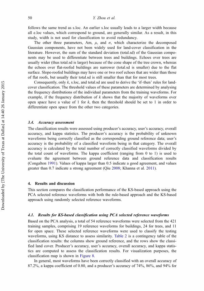
follows the same trend as s.loc. An earlier s.loc usually leads to a larger width becauseall e.loc values, which correspond to ground, are generally similar. As a result, in thisstudy, width is not used for classification to avoid redundancy.

The other three parameters, Am, μ, and σ, which characterize the decomposedGaussian components, have not been widely used for land-cover classification in theliterature. However, the sum of the standard deviation (total.sd) of the Gaussian compo-nents may be used to differentiate between trees and buildings. Echoes over trees areusually wider (thus total.sd is larger) because of the cone shape of the tree crown, whereasthe echoes over flat-roofed buildings are narrower (total.sd is smaller) due to the flatsurface. Slope-roofed buildings may have one or two roof echoes that are wider than thoseof flat roofs, but usually their total.sd is still smaller than that for most trees.

Consequently, only k, s.loc, and total.sd are used to derive the ‘if–then’ rules for land-cover classification. The threshold values of these parameters are determined by analysingthe frequency distributions of the individual parameters from the training waveforms. Forexample, if the frequency distribution of k shows that the majority of waveforms overopen space have a value of 1 for k, then the threshold should be set to 1 in order todifferentiate open space from the other two categories.

3.4. Accuracy assessment

The classification results were assessed using producer’s accuracy, user’s accuracy, overallaccuracy, and kappa statistics. The producer’s accuracy is the probability of unknownwaveforms being correctly classified as the corresponding ground reference data; user’saccuracy is the probability of a classified waveform being in that category. The overallaccuracy is calculated by the total number of correctly classified waveforms divided bythe total count of waveforms. The kappa coefficient (ranging from 0 to 1) is used toevaluate the agreement between ground reference data and classification results(Congalton 1991). Values of kappa larger than 0.5 indicate a good agreement, and valuesgreater than 0.7 indicate a strong agreement (Qiu 2008; Khanna et al. 2011).

4. Results and discussion

This section compares the classification performance of the KS-based approach using thePCA selected reference waveforms with both the rule-based approach and the KS-basedapproach using randomly selected reference waveforms.

4.1. Results for KS-based classification using PCA selected reference waveforms

Based on the PCA analysis, a total of 54 reference waveforms were selected from the 421training samples, comprising 19 reference waveforms for buildings, 24 for trees, and 11for open space. These selected reference waveforms were used to classify the testingwaveforms, using KS distance to assess similarity. Table 2 is a contingency table of theclassification results: the columns show ground reference, and the rows show the classi-fied land cover. Producer’s accuracy, user’s accuracy, overall accuracy, and kappa statis-tics are computed to assess the classification results. For visualization purposes, theclassification map is shown in Figure 8.

In general, most waveforms have been correctly classified with an overall accuracy of87.2%, a kappa coefficient of 0.80, and a producer’s accuracy of 74%, 86%, and 94% for

50 Y. Zhou et al.

Dow

nloa

ded

by [

The

Uni

vers

ity o

f T

exas

at D

alla

s] a

t 14:

40 2

6 Ja

nuar

y 20

15

Figure 8. The classification result of ICESat waveforms. (a) Map of classification for all footprintsin the study area. (b) The zoom-in map of the area within the yellow rectangle in (a) with thelatitude, longitude of its upper right corner being 32.915° N, ‒96.885° E.

Table 2. Confusion matrix of the KS-based approach.

Ground reference data

Classified data Building Tree Open space Producer’s accuracy (%) User’s accuracy (%)

Building 68 19 11 74 69Tree 22 116 0 86 84Open Space 2 0 185 94 99

Notes: Overall accuracy: 87.2%.Kappa coefficient: 0.80.

International Journal of Remote Sensing 51

Dow

nloa

ded

by [

The

Uni

vers

ity o

f T

exas

at D

alla

s] a

t 14:

40 2

6 Ja

nuar

y 20

15

building, tree, and open space categories, respectively, indicating a strong agreementbetween true ground references and classification results.

For buildings, 68 out of 92 waveforms were correctly classified. In the study area,most of the buildings were flat-roofed. Waveforms over the flat-roofed buildings usuallyshow two modes, one for the roof and the other for the ground. Both modes have anarrow echo width caused by their flat surfaces because, when the laser hits a flat roofor ground, a majority of the incoming pulses are reflected over a short time period. Thisleads to a narrow echo width with high amplitude of reflection in the waveform, whichin turn results in steep slopes in their associated CDF. This made it possible to separatewaveforms of flat-roofed buildings from those of trees. The buildings misclassified astrees were mainly slope-roofed, because their waveform curves were similar to those oftrees (Alexander et al. 2010). For trees, 19 out of 135 samples were misclassified asbuildings, most of which were low trees surrounding residential buildings, which wereconfused with the slope-roofed buildings. The open space had the highest accuracy(94%) among the three categories, although based on the smallest number of referencewaveforms. Waveforms for open space have the least variation in their curves, usuallywith a single mode and a narrow echo width. The small differences in their waveformslie primarily in the starting location and the amplitude of the wave caused by variationin open space elevation and surface conditions, respectively. As a result, they could beeasily differentiated from buildings and trees, both of which have a wider echo width,an earlier starting location and are multimodal. Only 11 open space waveforms weremisclassified as buildings, most of which were multiecho due to the existence of roughterrain or other objects within their footprints making their profiles similar to those oflow buildings.

4.2. Results for rule-based classification

For the rule-based approach, three parameters k (the number of Gaussian components),total.sd (the sum of the standard deviation of individual Gaussian components), and s.loc(the starting location of the noise-removed waveform) were used to derive the ‘if–then’classification rules, as discussed earlier.

Figure 9 presents the frequency distributions of k, total.sd, and s.loc of the samples inthe training data set. For the open space category, all three parameters are quite differentfrom those for the building and tree categories. This is especially true for k, which is largerthan 1 for all buildings and trees, whereas the vast majority of waveforms for open spaceare single-echo with k equal to 1. Therefore, the first classification rule was that, if kequals 1, the corresponding waveform is open space; otherwise, the waveform remainsunclassified. The parameter total.sd can be used to further separate the open space sampleswith more than one echo (k > 1) from the unclassified samples. A few waveforms for openspace were affected by slope or rough terrain, resulting in multiple, narrow-width echoes.However, the total.sd for most of these is smaller than 15 ns in the study area due to theirsmall number of echoes and narrow echo width, which was clearly different frombuildings and trees. After applying a second classification rule that, if total.sd < 15, thecorresponding waveform is also open space, the remaining unclassified samples weremostly trees and buildings.

Compared with open space, waveforms for buildings and trees are more complex,evidenced by the wide range and overlap of their three parameters. Consequently, acombination of parameters, rather than a single parameter, was required to differentiatebetween them. Since the trees in the study area were usually higher than buildings, and the

52 Y. Zhou et al.

Dow

nloa

ded

by [

The

Uni

vers

ity o

f T

exas

at D

alla

s] a

t 14:

40 2

6 Ja

nuar

y 20

15

cone shapes of tree crowns causes the tree waveforms to have wider echoes, most trees inthe study area have an earlier s.loc (<870 ns) and a larger total.sd (>30) than buildings.These two parameters were thus used to distinguish trees from buildings. The complete setof rules derived for land-cover classification is shown as a decision tree in Figure 10.

Table 3 presents the classification results using these rules. The rule-based approachperformed reasonably well with an overall accuracy of 83.7% and a kappa coefficient of0.75. It produced acceptable producer’s accuracies of 72% for buildings and 79% fortrees, with 16 out of 92 buildings misclassified as trees and 28 out of 135 treesmisclassified as buildings. This was primarily due to the overlaps in total.sd and s.locbetween buildings and trees, since these two categories have some waveforms with similarheights or vertical structures. This was particularly true for waveforms over slope-roofedresidential buildings surrounded by similar height or lower height trees, which results insimilar s.loc and total.sd values with trees of a similar height. These buildings have a highprobability of being misclassified as trees. As a consequence, the combined use of s.locand total.sd to discriminate buildings from trees met only with limited success. As foropen space, their waveforms usually have a single-echo due to the flat surface, with a few

200

150

100Fr

eque

ncy

Freq

uenc

yFr

eque

ncy

100

80

60

40

30

20

10

0

40

20

0

50

01

0

655

670

685

700

715

730

745

760

775

790

805

820

835

850

865

880

895

910

925

940

5 10 15 20 25 30 35 40total.sd (ns)

s.loc (ns)

45 50 55 60 65 70 75 80 85

2 3 4 5

k

6

Trees

Buildings

Open space

7 8 9 10

Figure 9. Frequency distributions of k (i.e. the number of Gaussian components), total.sd (i.e. thesum of standard deviation of the individual Gaussian components), and s.loc (starting location) oftraining samples.

International Journal of Remote Sensing 53

Dow

nloa

ded

by [

The

Uni

vers

ity o

f T

exas

at D

alla

s] a

t 14:

40 2

6 Ja

nuar

y 20

15

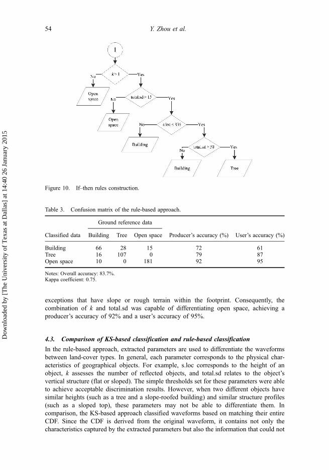
exceptions that have slope or rough terrain within the footprint. Consequently, thecombination of k and total.sd was capable of differentiating open space, achieving aproducer’s accuracy of 92% and a user’s accuracy of 95%.

4.3. Comparison of KS-based classification and rule-based classification

In the rule-based approach, extracted parameters are used to differentiate the waveformsbetween land-cover types. In general, each parameter corresponds to the physical char-acteristics of geographical objects. For example, s.loc corresponds to the height of anobject, k assesses the number of reflected objects, and total.sd relates to the object’svertical structure (flat or sloped). The simple thresholds set for these parameters were ableto achieve acceptable discrimination results. However, when two different objects havesimilar heights (such as a tree and a slope-roofed building) and similar structure profiles(such as a sloped top), these parameters may not be able to differentiate them. Incomparison, the KS-based approach classified waveforms based on matching their entireCDF. Since the CDF is derived from the original waveform, it contains not only thecharacteristics captured by the extracted parameters but also the information that could not

Figure 10. If–then rules construction.

Table 3. Confusion matrix of the rule-based approach.

Ground reference data

Classified data Building Tree Open space Producer’s accuracy (%) User’s accuracy (%)

Building 66 28 15 72 61Tree 16 107 0 79 87Open space 10 0 181 92 95

Notes: Overall accuracy: 83.7%.Kappa coefficient: 0.75.

54 Y. Zhou et al.

Dow

nloa

ded

by [

The

Uni

vers

ity o

f T

exas

at D

alla

s] a

t 14:

40 2

6 Ja

nuar

y 20

15

be represented by these parameters, such as the small local peaks, and the local skewnessand kurtosis that cannot be completely characterized by a few Gaussian components.Basically, the entirety of the information provided by the waveform is made available forclassification via the CDF. As a result, the KS-based approach was able to achieve betterperformance with a 3.5 percentage point improvement in overall accuracy, and 2, 7, and 2percentage point improvements in producer’s accuracy for building, tree, and open space,respectively, over the rule-based classification.

These numbers, although not large, do validate the superiority of the KS distanceapproach. However, an even more significant advantage of the KS approach is theabsence of any need for interpretation by analysts, which helps ensure consistency inclassification results. The rule-based approach requires the analysts to determine rulesbased on an inspection of parameter values, and there is no guarantee that two analystswould derive identical rules. The use of PCA, coupled with KS distance measures, forselection of the reference waveforms relies on a purely quantitative approach which willalways be duplicable given the same input data. Furthermore, the derivation of rules canbe very specific to the characteristics of the study area. This is evidenced by thediscussion of rule selection earlier, which references particular characteristics of ourstudy area, such as the large height of trees relative to buildings reflecting the maturityof these residential neighbourhoods. If the study area included newer neighbourhoodswith recently planted trees, these rules would likely require modification by the analysts.Using the PCA approach, these differences are automatically incorporated.

4.4. Results for KS-based classification using randomly selected reference waveforms

We also compared KS-based classification results using the PCA selected referencewaveforms with classification results using 10 trials of randomly selected referencewaveforms. The number of references for each category was kept the same as that forPCA selected references across all 10 trials, that is, 19 reference waveforms for buildings,24 for trees, and 11 for open space. The classification results (Table 4) indicate that thePCA selected reference waveforms consistently outperformed randomly selected

Table 4. Comparison of classification results.

Accuracy

Building(%)

Tree(%)

Open space(%)

Overall(%)

Randomly selected referencewaveforms

1th 54 79 88 78.02nd 66 82 93 83.73rd 61 81 86 79.04th 63 75 91 79.95th 66 84 93 84.46th 72 82 90 83.57th 64 80 94 83.28th 73 81 81 79.29th 68 81 89 81.810th 67 79 92 82.7std 5 2 4 2.3Average 66 80 90 81.5

PCA selected reference waveforms 74 86 94 87.2

International Journal of Remote Sensing 55

Dow

nloa

ded

by [

The

Uni

vers

ity o

f T

exas

at D

alla

s] a

t 14:

40 2

6 Ja

nuar

y 20

15

references. The overall accuracy of 87.2% for the PCA approach was higher than theoverall accuracy of any of the random selection trials. Nevertheless, the randomly selectedreferences were able to produce acceptable results with an average overall accuracy of81.5%. However, accuracy varied substantially between the land-cover classes. Theperformance for buildings was consistently the poorest among all categories in the 10trials, which resulted in the lowest average producer’s accuracy of 66% compared with74% for the PCA approach. Among all the building training samples, only a small numberwere slope-roofed residential buildings surrounded by trees of similar height. Randomreference selection missed picking up a reference for these buildings, causing many to bemisclassified as trees. For trees, the randomly selected references achieved consistent andrelatively accurate results for all 10 trials, with an average producer’s accuracy of 80%,compared with 86% for the PCA approach, and a small standard deviation of 2%. As foropen space, an average accuracy of 90% was achieved (with a minimum of 81% and amaximum of 94%) compared with 94% for the PCA approach. There are only a few openspace training samples having multiechoes due to the existence of rough terrain or otherobjects within the footprint. Missing references for these samples by the random selectionmethod is the likely cause of poorer classification results in some of the trials.

In general, the high variance of the producer’s accuracies (with standard deviations of5% and 4% for building and open space, respectively) suggests that the quality of theselected reference waveforms has an important impact on the classification results. It iscritical that the selected references for each category be able to adequately capture thewithin-class variation in the training data set. This is the main advantage of the PCA-based reference selection approach. The randomly selected references, on the contrary,may include many similar waveforms, but miss the ones with unique patterns due to alimited number of examples in the training data set. Compared to the randomly selectedreferences, the PCA selected references are capable of capturing the within-class varia-bility, which is critically important for methods based on curve matching.

5. Conclusions

In this study, we investigated the potential of using the ICESat waveform as a one-dimensional signal for land-cover classification over level terrain. For this purpose, the KSdistance is employed to measure the similarity between test waveforms and individualreference waveforms. The following conclusions can be drawn.

(1) Objects with distinct vertical structures (e.g. building, tree, and open space) withinthe ICESat footprint exhibit unique waveform curves that can be used to performland-cover classification.

(2) The use of the full-waveform curve to discriminate buildings, trees, and openspace over level terrain provides an alternative approach to existing metrics-basedmethods using a limited number of parameters (e.g. amplitude, width, number ofechoes, etc.) derived from the waveforms. By taking the full-waveform curve intoconsideration, the KS-based approach achieves a superior performance over thewidely adopted rule-based method, with the additional advantages of simplicity ofmathematical form, ease of implementation, no requirement for computationallycomplex Gaussian decomposition, and consistency of results stemming from thelack of need for analyst input.

(3) The references selected based on PCA play an important role in achieving betterclassification results compared with randomly selected references. Generally, the

56 Y. Zhou et al.

Dow

nloa

ded

by [

The

Uni

vers

ity o

f T

exas

at D

alla

s] a

t 14:

40 2

6 Ja

nuar

y 20

15

better the reference samples are able to capture within-class variability, the higherthe classification accuracies achieved by a curve matching approach.

(4) The utilization of full-waveform curve information is sufficient to separate objectswith distinct vertical structures. However, its ability to differentiate objects withsimilar vertical structures is limited. Future studies will focus on fusing full-waveform data and spectral data to perform fine-level land-cover classificationby taking advantage of both vertical structure information and surface spectralreflectance information.

(5) ICESat waveforms are sensitive to underlying terrain variation within the largefootprints (Hilbert and Schmullius 2012), which makes it challenging to applyboth KS-based and rule-based classification using ICESat waveform to slopedareas (slope > 15°). Future studies may focus on removing the terrain effects fromthe ICESat waveforms in advance and then evaluate the performance of curve-based approaches to waveform-based classification over slopes.

The use of ICESat waveforms for land-cover mapping is not likely to be widespread dueto the large spacing between its footprints along and between the tracts, and the presenceof mixed land covers within its large footprints. It was used here primarily to test a novelapproach to land-cover classification using full-waveform data and KS-distance-basedcurve matching. This approach will support the laser altimeter data expected from ICESat-2, the 2nd-generation ICESat mission scheduled for launch in early 2016. The approach isequally appropriate for feature extraction from small-footprint waveforms. More and moreairborne lidar systems now provide full waveforms with small footprints. These are likelyto have pure land-cover types in each footprint and minimal spacing between them. Thesewill be the focus of our future studies.

AcknowledgementsThe authors would like to thank the National Snow and Ice Data Center for providing ICESat data.

ReferencesAbbasi, M. K., M. Zafar, and S. R. Khan. 2007. “Influence of Different Land-Cover Types on the

Changes of Selected Soil Properties in the Mountain Region of Rawalakot Azad Jammu andKashmir.” Nutrient Cycling in Agroecosystems 78 (1): 97–110. doi:10.1007/s10705-006-9077-z.

Alexander, C., K. Tansey, J. Kaduk, D. Holland, and N. J. Tate. 2010. “Backscatter Coefficient as anAttribute for the Classification of Full-Waveform Airborne Laser Scanning Data in UrbanAreas.” ISPRS Journal of Photogrammetry and Remote Sensing 65 (5): 423–432.doi:10.1016/j.isprsjprs.2010.05.002.

Arroyo, L. A., K. Johansen, J. Armston, and S. Phinn. 2010. “Integration of LiDAR and QuickBirdImagery for Mapping Riparian Biophysical Parameters and Land Cover Types in AustralianTropical Savannas.” Forest Ecology and Management 259 (3): 598–606. doi:10.1016/j.foreco.2009.11.018.

Ballhorn, U., J. Jubanski, and F. Siegert. 2011. “ICESat/GLAS Data as a Measurement Tool forPeatland Topography and Peat Swamp Forest Biomass in Kalimantan, Indonesia.” RemoteSensing 3 (9): 1957–1982. doi:10.3390/rs3091957.

Boudreau, J., R. F. Nelson, H. A. Margolis, A. Beaudoin, L. Guindon, and D. S. Kimes. 2008.“Regional Aboveground Forest Biomass using Airborne and Spaceborne LiDAR in Québec.”Remote Sensing of Environment 112 (10): 3876–3890. doi:10.1016/j.rse.2008.06.003.

International Journal of Remote Sensing 57

Dow

nloa

ded

by [

The

Uni

vers

ity o

f T

exas

at D

alla

s] a

t 14:

40 2

6 Ja

nuar

y 20

15

Buddenbaum, H., S. Seeling, and J. Hill. 2013. “Fusion of Full-Waveform LiDAR and ImagingSpectroscopy Remote Sensing Data for the Characterization of Forest Stands.” InternationalJournal of Remote Sensing 34 (13): 4511–4524. doi:10.1080/01431161.2013.776721.

Burt, J., and G. Barber. 1996. Elementary Statistics for Geographers. New York: The GuildfordPress.

Cho, M. A., P. Debba, R. Mathieu, L. Naidoo, J. Van Aardt, and G. P. Asner. 2010. “ImprovingDiscrimination of Savanna Tree Species through a Multiple-Endmember Spectral Angle MapperApproach: Canopy-Level Analysis.” IEEE Transactions on Geoscience and Remote Sensing 48(11): 4133–4142.

Congalton, R. G. 1991. “A Review of Assessing the Accuracy of Classifications of RemotelySensed Data.” Remote Sensing of Environment 37 (1): 35–46. doi:10.1016/0034-4257(91)90048-B.

Dallmeyer, A., and M. Claussen. 2011. “The Influence of Land Cover Change in the AsianMonsoon Region on Present-Day and Mid-Holocene Climate.” Biogeosciences 8 (6): 1499–1519. doi:10.5194/bg-8-1499-2011.

Duncanson, L. I., K. O. Niemann, and M. A. Wulder. 2010. “Integration of GLAS and Landsat TMData for Aboveground Biomass Estimation.” Canadian Journal of Remote Sensing 36 (2): 129–141. doi:10.5589/m10-037.

Duong, H., R. Lindenbergh, N. Pfeifer, and G. Vosselman. 2009. “ICESat Full-Waveform AltimetryCompared to Airborne Laser Scanning Altimetry Over the Netherlands.” IEEE Transactions onGeoscience and Remote Sensing 47 (10): 3365–3378. doi:10.1109/TGRS.2009.2021468.

Duong, H., N. Pfeifer, and R. Lindenbergh. 2006. “Fullwaveform Analysis: ICESat Laser Data forLand Cover Classification.” In Proceedings of the ISPRS Mid-Term Symposium, RemoteSensing: From Pixels to Processes, Enschede, May 8–11, 30–35.

Farid, A., D. C. Goodrich, R. Bryant, and S. Sorooshian. 2008. “Using Airborne LiDAR to PredictLeaf Area Index in Cottonwood Trees and Refine Riparian Water-use Estimates.” Journal ofArid Environments 72 (1): 1–15. doi:10.1016/j.jaridenv.2007.04.010.

Fry, J. A., G. Xian, S. Jin, J. A. Dewitz, C. G. Homer, L. Yang, C. A. Barnes, N. D. Herold, and J.D. Wickham. 2011. “Completion of the 2006 National Land Cover Database for theConterminous United States.” Photogrammetric Engineering and Remote Sensing 77 (9):858–864.

Gong, P., Z. Li, H. Huang, G. Sun, and L. Wang. 2011. “ICESat GLAS Data for Urban EnvironmentMonitoring.” IEEE Transactions on Geoscience and Remote Sensing 49 (3): 1158–1172.doi:10.1109/TGRS.2010.2070514.

Grey, W. M. F., A. J. Luckman, and D. Holland. 2003. “Mapping Urban Change in the UK usingSatellite Radar Interferometry.” Remote Sensing of Environment 87 (1): 16–22. doi:10.1016/S0034-4257(03)00142-1.

Harding, D. J., and C. C. Carabajal. 2005. “ICESat Waveform Measurements of within-FootprintTopographic Relief and Vegetation Vertical Structure.” Geophysical Research Letters 32 (21):1–4. doi:10.1029/2005GL023471.

Harvey, K. R., and G. J. E. Hill. 2001. “Vegetation Mapping of a Tropical Freshwater Swamp in theNorthern Territory, Australia: A Comparison of Aerial Photography, Landsat TM and SPOTSatellite Imagery.” International Journal of Remote Sensing 22 (15): 2911–2925.

Hayashi, M., N. Saigusa, H. Oguma, and Y. Yamagata. 2013. “Forest Canopy Height EstimationUsing ICESat/GLAS Data and Error Factor Analysis in Hokkaido, Japan.” ISPRS Journal ofPhotogrammetry and Remote Sensing 81: 12–18. doi:10.1016/j.isprsjprs.2013.04.004.

Helmer, E. H., M. A. Lefsky, and D. A. Roberts. 2009. “Biomass Accumulation Rates ofAmazonian Secondary Forest and Biomass of Old-Growth Forests from Landsat Time Seriesand the Geoscience Laser Altimeter System.” Journal of Applied Remote Sensing 3: 1.

Hilbert, C., and C. Schmullius. 2012. “Influence of Surface Topography on ICESat/GLAS ForestHeight Estimation and Waveform Shape.” Remote Sensing 4 (8): 2210–2235. doi:10.3390/rs4082210.

Jawak, S. D., and A. J. Luis. 2013. “A Spectral Index Ratio-Based Antarctic Land-Cover Mappingusing Hyperspatial 8-Band World View-2 Imagery.” Polar Science 7 (1): 18–38. doi:10.1016/j.polar.2012.12.002.

Khanna, S., M. J. Santos, S. L. Ustin, and P. J. Haverkamp. 2011. “An Integrated Approach to aBiophysiologically Based Classification of Floating Aquatic Macrophytes.” InternationalJournal of Remote Sensing 32 (4): 1067–1094. doi:10.1080/01431160903505328.

58 Y. Zhou et al.

Dow

nloa

ded

by [

The

Uni

vers

ity o

f T

exas

at D

alla

s] a

t 14:

40 2

6 Ja

nuar

y 20

15

Lee, S., W. Ni-Meister, W. Yang, and Q. Chen. 2011. “Physically Based Vertical VegetationStructure Retrieval from ICESat Data: Validation using LVIS in White Mountain NationalForest, New Hampshire, USA.” Remote Sensing of Environment 115 (11): 2776–2785.doi:10.1016/j.rse.2010.08.026.

Lefsky, M. A., D. J. Harding, M. Keller, W. B. Cohen, C. C. Carabajal, F. Del Bom Espirito-Santo,M. O. Hunter, and R. de Oliveira Jr. 2005. “Estimates of Forest Canopy Height andAboveground Biomass using ICESat.” Geophysical Research Letters 32 (22): 1–4.doi:10.1029/2005GL023971.

Lefsky, M. A., M. Keller, Y. Pang, P. B. De Camargo, and M. O. Hunter. 2007. “Revised Method forForest Canopy Height Estimation from Geoscience Laser Altimeter System Waveforms.”Journal of Applied Remote Sensing 1: 1.

Li, L., S. L. Ustin, and M. Lay. 2005. “Application of Multiple Endmember Spectral MixtureAnalysis (MESMA) to AVIRIS Imagery for Coastal Salt Marsh Mapping: A Case Study inChina Camp, CA, USA.” International Journal of Remote Sensing 26 (23): 5193–5207.doi:10.1080/01431160500218911.

Liu, C., H. Huang, P. Gong, X. Wang, J. Wang, W. Li, C. Li, and Z. Li. 2014. “Joint Use of ICESat/GLAS and Landsat Data in Land Cover Classification: A Case Study in Henan Province,China.” IEEE Journal of Selected Topics in Applied Earth Observations and Remote Sensing.doi:10.1109/JSTARS.2014.2327032.

Mallet, C., F. Bretar, M. Roux, U. Soergel, and C. Heipke. 2011. “Relevance Assessment of Full-Waveform LiDAR Data for Urban Area Classification.” ISPRS Journal of Photogrammetry andRemote Sensing 66 (6): S71–S84. doi:10.1016/j.isprsjprs.2011.09.008.

Molijn, R. A., R. C. Lindenbergh, and B. C. Gunter. 2011. “ICESat Laser Full Waveform Analysisfor the Classification of Land Cover Types Over the Cryosphere.” International Journal ofRemote Sensing 32 (23): 8799–8822. doi:10.1080/01431161.2010.547532.

Muss, J. D., D. J. Mladenoff, and P. A. Townsend. 2011. “A Pseudo-Waveform Technique to AssessForest Structure using Discrete LiDAR Data.” Remote Sensing of Environment 115 (3): 824–835. doi:10.1016/j.rse.2010.11.008.

Narayanan, R., H. B. Kim, and G. Sohn. 2009. “Classification of SHOALS 3000 BathymetricLiDAR Signals using Decision Tree and Ensemble Techniques.” In TIC-STH’09: 2009 IEEEToronto International Conference – Science and Technology for Humanity, Toronto, ON,September 26–27, 462–467.

Nelson, R. 2010. “Model Effects on GLAS-Based Regional Estimates of Forest Biomass andCarbon.” International Journal of Remote Sensing 31 (5): 1359–1372. doi:10.1080/01431160903380557.

Nelson, R., K. J. Ranson, G. Sun, D. S. Kimes, V. Kharuk, and P. Montesano. 2009. “EstimatingSiberian Timber Volume using MODIS and ICESat/GLAS.” Remote Sensing of Environment113 (3): 691–701. doi:10.1016/j.rse.2008.11.010.

Oliver, J. J., R. A. Baxter, and C. S. Wallance. 1996. “Unsupervised Learning Using MML.”Proceedings of the Thirteenth International Conference on Machine Learning (ICML’96),Bari. July 3–6.

Pang, Y., M. Lefsky, G. Sun, and J. Ranson. 2011. “Impact of Footprint Diameter and Off-NadirPointing on the Precision of Canopy Height Estimates from Spaceborne LiDAR.” RemoteSensing of Environment 115 (11): 2798–2809. doi:10.1016/j.rse.2010.08.025.

Peerbhay, K. Y., O. Mutanga, and R. Ismail. 2013. “Commercial Tree Species Discrimination usingAirborne AISA Eagle Hyperspectral Imagery and Partial Least Squares Discriminant Analysis(PLS-DA) in KwaZulu-Natal, South Africa.” ISPRS Journal of Photogrammetry and RemoteSensing 79: 19–28. doi:10.1016/j.isprsjprs.2013.01.013.

Pirotti, F. 2010. “ICESat/GLAS Waveform Signal Processing for Ground Cover Classification: Stateof the Art.” Italian Journal of Remote Sensing/Rivista Italiana di Telerilevamento 42 (2): 13–26.doi:10.5721/ItJRS20104222.

Qiu, F. 2008. “Neuro-Fuzzy Based Analysis of Hyperspectral Imagery.” PhotogrammetricEngineering and Remote Sensing 74 (10): 1235–1247. doi:10.14358/PERS.74.10.1235.

Ranson, K. J., R. Nelson, D. Kimes, G. Sun, V. Kharuk, and P. Montesano. 2007. “Using MODISand GLAS Data to Develop Timber Volume Estimates in Central Siberia.” In 2007 IEEEInternational Geoscience and Remote Sensing Symposium, Barcelona, June 23–28, 2306–2309.

International Journal of Remote Sensing 59

Dow

nloa

ded

by [

The

Uni

vers

ity o

f T

exas

at D

alla

s] a

t 14:

40 2

6 Ja

nuar

y 20

15

Ranson, K. J., G. Sun, K. Kovacs, and V. I. Kharuk. 2004. “Landcover Attributes from ICESatGLAS Data in Central Siberia.” International Geoscience and Remote Sensing SymposiumProceedings 2: 753–756.

Rosette, J. A. B., P. R. J. North, and J. C. Suárez. 2008. “Vegetation Height Estimates for a MixedTemperate Forest using Satellite Laser Altimetry.” International Journal of Remote Sensing 29(5): 1475–1493. doi:10.1080/01431160701736380.

Rosso, P. H., S. L. Ustin, and A. Hastings. 2005. “Mapping Marshland Vegetation of San FranciscoBay, California, Using Hyperspectral Data.” International Journal of Remote Sensing 26 (23):5169–5191. doi:10.1080/01431160500218770.

Sarrazin, M. J. D., J. A. N. van Aardt, G. P. Asner, J. Mcglinchy, D. W. Messinger, and J. Wu. 2012.“Fusing Small-Footprint WaveformLiDAR and Hyper Spectral Data for Canopy-Level SpeciesClassification and Herbaceous Biomass Modeling in Savanna Ecosystems.” Canadian Journalof Remote Sensing 37 (6): 653–665. doi:10.5589/m12-007.

Sasaki, T., J. Imanishi, K. Ioki, Y. Morimoto, and K. Kitada. 2012. “Object-Based Classification ofLand Cover and Tree Species by Integrating Airborne LiDAR and High Spatial ResolutionImagery Data.” Landscape and Ecological Engineering 8 (2): 157–171. doi:10.1007/s11355-011-0158-z.

Sridharan, H., and F. Qiu. 2013. “Developing an Object-Based Hyperspatial Image Classifier with aCase Study Using WorldView-2 Data.” Photogrammetric Engineering & Remote Sensing 79(11): 1027–1036.

Sugumaran, R., and M. Voss. 2007. “Object-Oriented Classification ofLiDAR-Fused HyperspectralImagery for Tree Species Identification in an Urban Environment.” Paris 11: 1–6.

Sun, G., K. J. Ranson, D. S. Kimes, J. B. Blair, and K. Kovacs. 2008. “Forest Vertical Structurefrom GLAS: An Evaluation Using LVIS and SRTM Data.” Remote Sensing of Environment 112(1): 107–117.

Ussyshkin, V., and L. Theriault. 2011. “Airborne LiDAR: Advances in Discrete Return Technologyfor 3D Vegetation Mapping.” Remote Sensing 3 (3): 416–434.

Vögtle, T., and E. Steinle. 2003. “On the Quality of Object Classification and Automated BuildingModeling Based on Laserscanning Data.” The International Archives of the Photogrammetry,Remote Sensing and Spatial Information Sciences 34: 149–155.

Wang, X., X. Cheng, Z. Li, H. Huang, Z. Niu, X. Li, and P. Gong. 2012. “Lake Water FootprintIdentification from Time-Series ICESat/GLAS Data.” IEEE Geoscience and Remote SensingLetters 9 (3): 333–337.

Wang, X., H. Huang, P. Gong, C. Liu, C. Li, and W. Li. 2014. “Forest Canopy Height Extraction inRugged Areas With ICESat/GLAS Data.” IEEE Transactions on Geoscience and RemoteSensing 52 (8): 4650–4657.

Wu, H., and Y. Xing. 2010. “Comparison between ETM+ Imageries and ICESat-GLAS Waveformsfor Forest Classification.” In 2nd International Conference on Information Science andEngineering, Hangzhou, December 4–6, 1088–1092.

Zaletnyik, P., S. Laky, and C. Toth. 2010. “LIDAR Waveform Classification Using Self-OrganizingMap.” In American Society for Photogrammetry and Remote Sensing Annual Conference, SanDiego, CA, April 26–30, 1055–1066.

Zhang, J., A. de Gier, Y. Xing, and G. Sohn. 2011. “Full Waveform-Based Analysis for Forest TypeInformation Derivation from Large Footprint Spaceborne LiDAR Data.” PhotogrammetricEngineering and Remote Sensing 77 (3): 281–290.

Zhou, W., and A. Troy. 2008. “An Object-Oriented Approach for Analysing and CharacterizingUrban Landscape at the Parcel Level.” International Journal of Remote Sensing 29 (11): 3119–3135.

60 Y. Zhou et al.

Dow

nloa

ded

by [

The

Uni

vers

ity o

f T

exas

at D

alla

s] a

t 14:

40 2

6 Ja

nuar

y 20

15