ICES REPORT 17-11

May 2017

A framework for designing patient-specific bioprostheticheart valves using immersogeometric fluid–structure

interaction analysisby

Fei Xu, Simone Morganti, Rana Zakerzadeh, David Kamensky, Ferdinando Auricchio, Alessandro Reali,

Thomas J.R. Hughes, Michael S. Sacks, and Ming-Chen Hsu

The Institute for Computational Engineering and SciencesThe University of Texas at AustinAustin, Texas 78712

Reference: Fei Xu, Simone Morganti, Rana Zakerzadeh, David Kamensky, Ferdinando Auricchio, AlessandroReali, Thomas J.R. Hughes, Michael S. Sacks, and Ming-Chen Hsu, "A framework for designing patient-specificbioprosthetic heart valves using immersogeometric fluid–structure interaction analysis," ICES REPORT 17-11,The Institute for Computational Engineering and Sciences, The University of Texas at Austin, May 2017.

A framework for designing patient-specific bioprosthetic heartvalves using immersogeometric fluid–structure interaction analysis

Fei Xua, Simone Morgantib, Rana Zakerzadehc, David Kamenskyd, Ferdinando Auricchioe,Alessandro Realie, Thomas J.R. Hughesc, Michael S. Sacksc, Ming-Chen Hsua,∗

aDepartment of Mechanical Engineering, Iowa State University, 2025 Black Engineering, Ames, IA 50011, USAbDepartment of Electrical, Computer, and Biomedical Engineering, University of Pavia, via Ferrata 3, 27100, Pavia,

ItalycThe Institute for Computational Engineering and Sciences, The University of Texas at Austin, 201 East 24th St, Stop

C0200, Austin, TX 78712, USAdDepartment of Structural Engineering, University of California, San Diego, 9500 Gilman Drive, Mail Code 0085,

La Jolla, CA 92093, USAeDepartment of Civil Engineering and Architecture, University of Pavia, via Ferrata 3, 27100, Pavia, Italy

Abstract

Numerous studies have suggested that using medical images to construct computational mechan-ics models could reduce mortality and morbidity due to cardiovascular diseases by allowing forpatient-specific surgical planning or even customized design of medical devices. In this work,we present a novel framework for designing patient-specific prosthetic heart valves using a para-metric design platform and immersogeometric fluid–structure interaction (FSI) analysis. Theleaflet geometry is parameterized using several key design parameters. This allows for gener-ating various perturbations of the leaflet design for the patient-specific aortic root reconstructedfrom the medical image data. Each design is analyzed using our hybrid arbitrary Lagrangian–Eulerian/immersogeometric FSI methodology, which allows us to efficiently simulate the couplingof the deforming aortic root, the parametrically designed prosthetic valves, and the surroundingblood flow under physiological conditions. A parametric study is carried out to investigate the in-fluence of the geometry on heart valve performance, indicated by the effective orifice area (EOA)and the coaptation area (CA). Finally, the FSI simulation result of a design that balances EOA andCA reasonably well is compared with patient-specific phase contrast magnetic resonance imagingdata to demonstrate the qualitative similarity of the flow patterns in the ascending aorta.

Keywords: Bioprosthetic heart valves; Patient-specific; Fluid–structure interaction;Immersogeometric analysis; Isogeometric analysis; Parametric design

∗Corresponding authorEmail address: jmchsu@iastate.edu (Ming-Chen Hsu)

Preprint submitted to International Journal for Numerical Methods in Biomedical Engineering May 13, 2017

Contents

1 Introduction 2

2 Modeling and simulation framework 62.1 Patient-specific geometry modeling . . . . . . . . . . . . . . . . . . . . . . . . . 6

2.1.1 Patient-specific medical image processing . . . . . . . . . . . . . . . . . . 62.1.2 Trivariate NURBS parameterization of the ascending aorta . . . . . . . . . 72.1.3 Parametric BHV design . . . . . . . . . . . . . . . . . . . . . . . . . . . 9

2.2 Fluid–structure interaction problem . . . . . . . . . . . . . . . . . . . . . . . . . 112.3 Structural formulations . . . . . . . . . . . . . . . . . . . . . . . . . . . . . . . . 13

2.3.1 Artery wall modeling . . . . . . . . . . . . . . . . . . . . . . . . . . . . . 132.3.2 Thin shell formulations for the leaflets . . . . . . . . . . . . . . . . . . . . 142.3.3 Leaflet–artery coupling . . . . . . . . . . . . . . . . . . . . . . . . . . . . 16

2.4 Fluid formulation . . . . . . . . . . . . . . . . . . . . . . . . . . . . . . . . . . . 172.5 Time integration and discretization of fluid–structure coupling . . . . . . . . . . . 18

3 Application to BHV design 193.1 Effective orifice area . . . . . . . . . . . . . . . . . . . . . . . . . . . . . . . . . 193.2 Coaptation area . . . . . . . . . . . . . . . . . . . . . . . . . . . . . . . . . . . . 203.3 Simulation setup . . . . . . . . . . . . . . . . . . . . . . . . . . . . . . . . . . . 213.4 Parametric study . . . . . . . . . . . . . . . . . . . . . . . . . . . . . . . . . . . 22

4 Comparison with patient-specific image data 264.1 Post-processing phase contrast magnetic resonance images . . . . . . . . . . . . . 26

5 Conclusions 28

1. Introduction

Computer simulations of fluid and solid mechanics greatly expand the scope of what can be in-ferred from non-invasive imaging of the cardiovascular system. This claim has been argued by aca-demic researchers for about 20 years, starting with work of Taylor and collaborators [1, 2], but therecent entry of computational fluid dynamics (CFD) into mainstream clinical practice, as a methodof estimating fractional flow reserve (FFR) from computed tomography angiography (CTA) [3, 4],has decisively proven that the paradigm of image-based predictive modeling of the cardiovascularsystem can simultaneously improve diagnoses and outcomes while reducing costs. However, the

2

use of image-based CFD to circumvent costly invasive measurements of clinical quantities of in-terest realizes only a fraction of the potential benefits outlined in Taylor et al.’s proposed paradigmof predictive cardiovascular medicine [5]. Over the past decade or so, numerous studies havesuggested that using medical images to construct computational mechanics models could reducemortality and morbidity due to cardiovascular diseases by allowing for patient-specific surgicalplanning [6–12] or even customized design of medical devices [13–17].

The possibility of patient-specific device design is the topic of the present study. In particular,we focus on the potential role of computational fluid–structure interaction (FSI) analysis in thedesign of stentless aortic valve prostheses that conform to the aortic root geometries of individ-ual patients, as obtained from non-invasive CTA. Aortic valve replacement is commonly indicatedfor patients suffering from heart valve diseases; over 90,000 prosthetic valves are implanted inthe United States each year [18]. While valves can sometimes be surgically repaired, prostheticreplacement is the only option for a vast majority of patients [19]. Replacement heart valves fab-ricated from biologically derived materials are referred to as bioprosthetic heart valves (BHVs).While these devices have blood flow characteristics similar to the native valves, device failurecontinues to result from leaflet structural deterioration, mediated by fatigue and/or tissue miner-alization. Mechanical stress has long been known to play a role in this deterioration [20] andsubstantial work has been done by academic researchers to predict and optimize the distributionof this stress by using tools from engineering analysis to simulate (quasi-)static [21] and dynamic[22] structural mechanics, and, more recently, fluid–structure interaction (FSI) [23].

Most BHVs consist of chemically-fixed soft-tissue leaflets sutured to a rigid stent [24]. Stentsare available in multiple sizes, but this several-sizes-fit-all paradigm may not provide optimal re-sults for many patients since valve performance is highly dependent on the geometry of the rootand the leaflets. Alternatives to rigid stented valves include stentless valves [24], offering largerorifice areas and improved hemodynamics. However, as stated by Xiong et al. [25], the prostheticleaflet geometry of a stentless valve plays a key role for its efficacy and durability. Auricchio et al.[15] found that geometrically symmetric stentless prosthetic valves implanted in patient-specificaortic roots, in general characterized by asymmetric sinuses, can cause heart valve misclosure,leading to valve insufficiency. Clinical aspects of stentless valves are reviewed in Ennker et al.[26]. The cited study concluded that stentless valves “decreased incidence of patient–prosthesismismatch” [26, pp. 81] and that “A survival advantage for stentless bioprostheses in comparison tostented ones has been reported by all studies in the literature” [26, pp. 77]. However, the authorsalso noted that “despite proper training and the development of routines, many surgeons are re-luctant to perform the total root technique (or stentless valve implantation at all)” [26, pp. 79–80],due to the technical complexity of the operation. The implantation technique is non-trivial andtherefore the clinical outcomes of these implants are strongly dependent on an appropriate choice

3

of both prosthesis size and replacement technique, which is, at present, strictly related to the sur-geon’s experience and skill [27]. In the present study, we propose a patient-specific computationalapproach to support pre-operative planning of stentless aortic valve implants by studying the sensi-tivity of prosthesis geometric features and determining the best-performing prosthesis shape. Moreprecisely, we hypothesize that image-based patient-specific computational FSI analysis could pro-vide a rational method for planning and optimizing the details of this complex surgery in advance,increasing the probability of realizing the full benefits of stentless valve replacement.

The construction of geometrical computer models of heart valves is already attracting interestfrom the medical device industry. For example, the Siemens eSie Valves system [28] is marketed asa means for physicians to extract geometrical quantities of interest (e.g., annulus diameter, orificearea, etc.) from medical images of patients’ heart valves. Desirable features of such a system areclosely aligned with those of computer-aided design (CAD) programs used in engineering. Forinstance, a recent white paper [29] on the eSie Valves technology emphasizes the importance of“intuitive editing” of semi-automatically-generated segmentations of patients’ valve leaflets. If wewant to develop computational mechanics analysis technologies that align with this trend, we arenaturally led to the field of isogeometric analysis (IGA).

Isogeometric analysis was originally proposed by Hughes et al. [30] as a way to unify engineer-ing analysis and design, by directly employing designer-friendly representations of geometry ascomputational analysis models. This eliminates the difficult task of converting between design ge-ometries and finite element/volume representations needed for numerical analysis. As mentionedabove, clinicians would prefer design-like representations of geometry that can be intuitively ma-nipulated. Obtaining these representations from medical images is itself nontrivial, but one can atleast avoid doubling the segmentation workload by leveraging IGA to re-use these representationsas analysis models. Image-based patient-specific IGA of heart valve structural mechanics has beenpreviously studied by Morganti et al. [31], who found that IGA of heart valves does not just per-mit convenient re-use of intuitive geometry representations; it can also dramatically increase theaccuracy of mechanical analyses relative to traditional finite element discretizations [31, Figures13 and 14]. The current contribution extends this body of work on patient-specific heart valve IGAto include FSI analysis. Due to the difficulty of developing general-purpose methods for trackingfluid–solid interfaces through large and complex deformations, such as those undergone by aorticvalve leaflets, we have combined ideas from IGA with the concept of immersed boundary FSIanalysis [32]. We refer to this combination of ideas as immersogeometric FSI analysis [33].

Immersogeometric analysis is ideally-suited to automatic optimization of engineered systemsand/or exploration of design spaces, as it directly immerses CAD boundary representations of en-gineering designs into unfitted discretizations of volumes [34, 35]. CAD geometries are oftenparameterized in terms of a few key dimensions; this is known as parametric design. Using tradi-

4

tional finite element or finite volume analysis methods, one would need to regenerate an analysismesh every time a design parameter is modified, which often requires some manual interventionby the analyst. Using immersogeometric approaches, design parameters can be varied freely, andthe modified design can be re-analyzed without human intervention. This is demonstrated by theparametric design optimization of a water brake in Wu et al. [36]. The idea of applying immerso-geometric FSI analysis to a parametric BHV design is shown in Hsu et al. [37].

Parametric design of heart valve leaflet geometries dates back to Thubrikar [38, Chapter 1],which introduced a 3D geometry description of the aortic valve by considering the intersectionsurfaces of a cone with inclined planes and used this description to search for optimal prostheticdimensions with appropriate coaptation, minimum volume, and efficient use of energy. Subsequentstudies on parameterized heart valve geometries include Labrosse et al. [39], Auricchio et al. [15],Haj-Ali et al. [40], Kouhi and Morsi [41], and Li and Sun [42]. These studies have focused ondefining general guidelines for prosthetic valve design that might be expected to improve averageoutcomes for the population considered as a whole. However, with the advent of 3D bioprinting[43] (which has already been studied in the context of aortic valve replacement [44]), it may soonbe possible to perform optimization of geometry on a per-patient basis, taking into account vari-ations in patient aortic root geometry and other patient-specific factors. Computational methodsenabling patient-specific simulations of native and prosthetic heart valves were reviewed by Vottaet al. [45] in 2013. To the best of our knowledge, a systematic patient-specific parametric studythat examines the effect of leaflet’s shape on the prosthetic valve performance has not yet beencarried out.

In this work, we develop a framework for designing patient-specific prosthetic heart valvesusing an IGA-based parametric design platform and immersogeometric FSI analysis. The patient-specific aortic root geometry is reconstructed from the medical image data and is represented us-ing non-uniform rational B-splines (NURBS). The leaflet geometry is parameterized using severalgeometric design parameters which allows for generating various perturbations of the leaflet de-sign for the patient’s aortic root. Each design is analyzed using our hybrid arbitrary Lagrangian–Eulerian/immersogeometric FSI solver, which allows us to efficiently perform a computation thatcombines a boundary-fitted, deforming-mesh treatment of the artery with a non-boundary-fittedtreatment of the leaflets. We simulate the coupled dynamics of the patient-specific aortic root,parametrically designed heart valves, and surrounding blood flow, under physiological conditions.The leaflet and arterial wall motion are coupled using a penalty formulation imposed over theleaflet–wall intersection. The artery wall tissue prestress is included to improve the physical real-ism of the modeling. A parametric study is carried out to investigate the influence of the geometryon heart valve efficiency and performance, indicated by the effective orifice area (EOA) during theopening phase and the coaptation area (CA) during the closing phase, and to identify a design that

5

balances EOA and CA reasonably well. Finally, the simulation result of this best-performing pros-thetic valve is compared with the phase contrast magnetic resonance imaging (PC-MRI) data fromthe patient to demonstrate the qualitative similarity of the flow patterns in the ascending aorta.

The paper is organized as follows. In Section 2, we describe the tools that we use to performpatient-specific valve simulations: Section 2.1 introduces our techniques for obtaining spline-basedgeometrical representations of arteries and valves, using medical image processing and parametricdesign; Sections 2.2–2.5 cover the mathematical models of continuum mechanics that we assumefor the fluid and structural components, and our isogeometric and immersogeometric discretiza-tions of those models. In Section 3, we explore the parametric BHV design space and evaluatescandidate valves in terms of clinical quantities of interest. In Section 4, we compare simulatedhemodynamics with patient-specific magnetic resonance velocimetry data. Finally, the conclu-sions are presented in Section 5.

2. Modeling and simulation framework

This section describes our pipeline for processing medical image data into geometrical modelsof the ascending aorta, parameterizing patient-specific BHV design spaces, and discretizing FSIproblems posed on these custom geometries.

2.1. Patient-specific geometry modeling

We demonstrate our geometrical modeling approach using ECG-gated CTA and PC-MRI ofthe aortic valve region of a 69 year-old patient. This data was obtained from the internal databaseof the IRCCS Policlinico San Donato hospital in Milan, Italy. The selected patient underwentradiological investigations for descending aorta disease, while being characterized as having ahealthy aortic valve. This and the amount of available imaging data are the main reasons forchoosing this specific patient.

2.1.1. Patient-specific medical image processing

Contrast enhanced multislice CTA was performed using a Siemens SOMATOM Definition ASscanner (Siemens Medical Solutions, Erlangen, Germany), with a collimation width of 0.6 mm,slice thickness of 0.75 mm, and pixel spacing of 0.685 mm × 0.685 mm. We process CTA imagesusing the open-source Vascular Modeling ToolKit (vmtk) [46] to segment the aortic root fromthe left ventriculo-aortic junction to the sinotubular one. CTA images from end diastole havethe highest quality and are therefore selected for segmentation. We use level sets following theapproach proposed by Antiga et al. [47]. After completing the segmentation step, a triangulatedsurface representation of the aortic lumen is obtained using the marching cubes algorithm. Acenterline of the aortic root segment is computed from its surface model using vmtk. A simple and

6

(a) (b) (c)

Figure 1: (a) The NURBS surface representation of the patient-specific aortic root. (b) The NURBS surfaces of theascending aorta. The lumen surface (or the inner artery wall surface) is shown in red and the outer artery wall surfaceis shown in gray. (c) The control points and control mesh of the outer artery wall surface.

fast least-squares approach is then adopted to map a primitive NURBS geometry (e.g., a cylinder)onto the obtained target lumen surface representation. We refer readers to Morganti et al. [31]for more details on this procedure. Finally, the quadratic NURBS surface representation of thepatient-specific aortic root is shown in Figure 1a.

In this work, we plan to simulate the blood flow in a deforming ascending aorta interacting withdifferent designs of the BHV. To do so, we first add a short tubular extension between the aorticroot and the left ventricle, and a longer tubular extension between the aortic root and the arch.This gives us the lumen surface of our ascending aorta, extended from the patient-specific aorticroot geometry. For the purpose of constructing a 3D discretization of the artery wall, we expandthe lumen surface in the outward normal direction to obtain a model of the outer surface of theaortic wall. (As a result, the lumen surface also serves as the inner surface of the aortic wall.) Forsimplicity, we choose a constant wall thickness of 2.5 mm, which is in the range of physiologicalvalues [48]. The final NURBS surfaces of the ascending aorta are shown in Figure 1b. The controlpoints and control mesh of the outer surface are shown in Figure 1c. The NURBS inner and outersurfaces are used to construct volumetric NURBS descriptions of the fluid (lumen) and solid (arterywall) domain geometries that are suitable for isogeometric analysis.

2.1.2. Trivariate NURBS parameterization of the ascending aorta

To obtain a volumetric parameterization of the artery and lumen, we first construct a trivariatemulti-patch NURBS in a regular shape, e.g. a tubular domain, with lateral boundaries and an inter-nal hypersurface that have the same control mesh topologies as the outer and inner surfaces of the

7

artery wall shown in Figure 1b. We then solve a linear elastostatic, mesh moving problem [49–51]for the displacement from this regular domain to a deformed configuration that represents the arteryand lumen. The control points shown in Figure 1c are used to prescribe Dirichlet boundary con-ditions on the displacement of the regular domain’s lateral boundaries and internal hypersurface.However, solving a linear elastostatic problem to obtain the deformed interior mesh is only effec-tive for relatively mild or translational deformations. For scenarios that involve large rotationalstructural motions, such as the deformation of a straight tubular domain into the curved shape ofpatient-specific ascending aorta in Figure 1b, the interior elements can become severely distorted.To avoid this, we construct the initial regular domain in the following way.

We first obtain a centerline along the axial direction of the patient-specific artery wall surface.Along this centerline, we define a number of cross sections corresponding to the control pointsof the NURBS artery wall surface in the axial direction. (These cross sections are shown as bluecurves in Figure 2a.) At each cross section, we calculate its unit normal vector nc and the effectiveradius rc, which is determined such that the area of a circle calculated using this radius matches thearea of the cross section. (A circle corresponding to one of the cross sections is shown in the redcurve in Figure 2a.) Finally, using this information, we construct a tubular NURBS surface that hasthe same control point and knot vector topology as the target patient-specific artery wall surface,as shown in Figures 2b and 2c. Another tubular surface corresponding to the lumen surface isalso constructed, using the same cross sections but smaller effective radii coming from the lumenNURBS surface.

These two tubular NURBS surfaces are used to construct a primitive trivariate multi-patchNURBS that includes (pre-images of) the solid and fluid subdomains, shown in gray and red,respectively, in Figure 2d. The multi-patch design avoids the parametric degeneracy that wouldoccur in a cylindrical-polar single-patch parameterization. Due to this, a total of six C0-continuouslocations are present in the circumferential direction of the NURBS domain.1 Basis functionsare made C0-continuous at the fluid–solid interface, so that velocity functions defined using theresulting spline space conform to standard fluid–structure kinematic constraints while retainingthe ability to represent non-smooth behavior across the material interface.

The resulting volumetric NURBS can then be morphed to match the patient-specific geometrywith minimal rotation, so an elastostatic problem can provide an analysis-suitable parameteriza-tion. Mesh quality is further enhanced by including Jacobian-based stiffening techniques [53], toavoid excessive distortion of small elements in critical areas such as the vicinity of the fluid–solidinterface. Displacements at the ends of the tube are constrained to remain within their respective

1It is in fact possible to define an arbitrarily-smooth spline space over the entire tubular volume, by leveragingrecent progress on polar splines [52], but we require only C0 continuity for the analysis methods used in the presentwork.

8

ncrc

(a) Cross sections of the artery wall sur-face

(b) Circular cross sections (c) NURBS tubular surface andcorresponding control points

(d) Primitive volume mesh (e) Deformed volume mesh (f) h-refined volume mesh

Figure 2: The construction of the volumetric NURBS discretization of the blood and the artery wall domains.

cross sections. Finally, we refine the deformed trivariate NURBS for analysis purposes, by insert-ing knots at desired locations, such as around the sinuses and the flow boundary layers. The finalvolumetric NURBS discretization of the patient-specific ascending aorta is shown in Figure 2f. Themesh of the lumen and artery wall consist of 58,752 and 6,912 quadratic elements, respectively.

2.1.3. Parametric BHV design

In this paper, we aim to advance methods for designing effective prosthetic valves for specificpatients. This requires the capability to control the design of aortic valve leaflets within the geo-metrical constraints imposed by an arbitrary patient-specific aortic root. Starting from the NURBSsurface of a patient-specific root, valve leaflets are parametrically designed as follows. We first picknine “key points” located on the ends of commissure lines and the bottom of the sinuses. These

9

p1p2

p3

p4

Figure 3: The key geometric features used to parametrically control the valve designs. The blue key points define theattachment of the valve to the root. The red and green curves are parametrically controlled for valve design.

define how the leaflets attach to the sinuses (Figure 3). The key points solely depend on the geom-etry of the patient-specific aortic root and will remain unchanged for different valve designs. Wethen parameterize families of univariate B-splines defining the free edges and radial “belly curves”of the leaflets. These curves are shown in red and green in Figure 3. The attachment edges, freeedges, and belly curves are then interpolated to obtain smooth bivariate B-spline representationsof the leaflets.

Figure 4 shows the details of parameterizing the free-edge curve (red) and the belly-regioncurve (green). We take one of the three leaflets to address the parameters controlling the valvedesigns. In Figure 4, p1, p2 and p3 are the key points on the top of the commissure lines and p4

is the key point on the sinus bottom. p1 to p3 define a triangle ∆p1–3, with pc being its geometriccenter. The unit vector pointing from pc to pn (the geometric center of p1 and p2) is denoted astp, and the unit normal vector of ∆p1–3 pointing downwards is np. We first construct the free edgecurve as a univariate quadratic B-spline curve determined by three control points, p1, pf, and p2.pf is defined by pf = pc + x1tp + x2np. By changing x1 and x2 to control the location of pf, thecurvature (length) and the height of the free edge can be parametrically changed. We then takepm as the midpoint of the free edge, the point pb, and the key point p4 to construct a univariatequadratic B-spline curve (green). The point pb is defined by pb = po + x3np, where po is theprojection of pm onto ∆p1–3 along the direction of np. The physical meaning of x3 is the verticaldistance between pb and ∆p1–3. Thus, the free edge and the belly curve share the point pm in thephysical space. Note that the aforementioned control points are used to construct the curves onlyand are not the control points of the final surface. Finally, the fixed attachment edges and theparametrically controlled free edge and belly curve are used to construct a cubic B-spline surfacewith desired parameterization.

10

p1

p3

pc

pm

p4

pf

pb

x2np

x3np

po

pnp2

Figure 4: The parametric control of the valve designs. x1, x2, and x3 control the location of Pf and Pb and thus controlthe curvature and height of the red free edge, and the curvature of the green belly curve.

Figure 5: User interface for the parametric design tool of the valve designs. Design variables x1, x2, and x3 are listedas “Parametric control”.

By choosing x1, x2 and x3 as design variables, we can parametrically change the free edgeand belly curve, and therefore change the valve design. This procedure is implemented in aninteractive geometry modeling and parametric design platform [54] based on Rhinoceros 3D [55]and Grasshopper [56], and demonstrated in Figure 5. Some sample points in the design space aredepicted in Figure 6, to illustrate the effect of each parameter on the geometry. Four examples ofheart valve designs are shown in Figure 7.

2.2. Fluid–structure interaction problem

We model the ascending aorta and prosthetic valve leaflets at time t as elastic structures occu-pying a region (Ωs)t, coupled to blood flow through (Ωf)t by kinematic and traction compatibilityconditions at the fluid–structure interface (ΓI)t. The blood flow within (Ωf)t is assumed to be in-compressible and Newtonian. The subscript t may be omitted in some formulas below, when thereis no risk of confusion. This coupled PDE system can be expressed in weak form as: Find a fluidvelocity uf ∈ Su and pressure p ∈ Sp, a structural displacement field y ∈ Sy, and a fluid–solid

11

P1

P3P2

P4

(a) Increasing x1

P1 (P2)

P4

P3

(b) Increasing x2

P1 (P2) P3

P4

(c) Increasing x3

Figure 6: The effect of increasing design parameters x1, x2, and x3. Red surfaces denote designs before increasing thedesign parameters and green surfaces denote designs after increasing the design parameters.

(a) (b) (c) (d)

Figure 7: Selected examples of the heart valve designs used in this work. (a) x1 = 0.05 cm, x2 = 0.1 cm, and x3 = 0.8cm. (b) x1 = 0.45 cm, x2 = 0.1 cm, and x3 = 0.8 cm. (c) x1 = 0.05 cm, x2 = 0.5 cm, and x3 = 0.8 cm. (d) x1 = 0.05cm, x2 = 0.1 cm, and x3 = 1.4 cm.

interface traction λλλ ∈ S` such that for all wf ∈ Vu, q ∈ Vp, ws ∈ Vy, and δλλλ ∈ Vl,

Bf(wf, q, uf, p) − Ff(wf, q) + Bs(ws, y) − Fs(ws)

+

∫ΓI

(wf − ws) · λλλ dΓ +

∫ΓI

δλλλ · (uf − us) dΓ

+

∫ΓI

(wf − ws) · β (uf − us) dΓ = 0 , (1)

where S(·) and V(·) are trial solution and test function spaces, Bf, Ff, Bs, and Fs are variationalforms defining the fluid and structure subproblems, us is the material time derivative of y, and β isa penalty parameter. The additional terms integrated over ΓI enforce the fluid–structure couplingconditions on the fluid–structure interface2. The presence of the last term facilitates the develop-ment of certain numerical schemes based on the “augmented Lagrangian” concept, as detailed inBazilevs et al. [57, Section 2]. The forms defining the fluid and structure subproblems are specified

2If the fluid and structural velocities and test functions are explicitly assumed to be continuous (i.e., uf = us andwf = ws) at the interface (e.g., matching lumen and inner artery wall surface meshes), these additional terms integratedover ΓI are zero.

12

in the sequel.

2.3. Structural formulations

The artery wall is substantially thicker than the valve leaflets. We model the artery wall asan elastic solid and we model the valve leaflets as a thin shell structure. This distinction can beformalized by introducing superscripts “so” and “sh” to denote the solid and shell, respectively,and expressing Sy = Sso

y × Sshy and Vy = Vso

y × Vshy , such that y =

yso, ysh

and ws =

wso

s ,wshs

.

We can then writeBs (ws, y) = Bso

s(wso

s , yso) + Bsh

s

(wsh

s , ysh)

, (2)

and likewise for Fs.

Remark 1. In a slight abuse of notation, linear combinations of ws and y with functions definedon the fluid domain (as seen in the fluid–structure interface terms of (1)) are understood to involveonly whichever component of the structure trial/test function tuple is defined at a given point onΓI.

2.3.1. Artery wall modeling

The artery wall is modeled as a hyperelastic solid, subject to damping forces. We thus define

Bsos (ws, y) − Fso

s (ws)

=

∫(Ωso

s )t

ws · ρs∂2y∂t2

∣∣∣∣∣∣X

dΩ +

∫(Ωso

s )0

∇∇∇Xws : F (S + S0) dΩ

−

∫(Ωso

s )t

ws · ρsfs dΩ −

∫(Γ

so,hs

)t

ws · hs dΓ , (3)

where Ωsos is the portion of Ωs corresponding to the artery wall, ρs is the solid mass density, X

are coordinates in the reference configuration, F is the deformation gradient associated with dis-placement y, S is the hyperelastic contribution to the second Piola–Kirchhoff stress tensor, S0 is aprescribed prestress in the reference configuration

(Ωso

s)

0, fs is a prescribed body force, and hs is aprescribed traction on the Neumann boundary Γso,h

s . The elastic contribution to the second Piola–Kirchhoff stress in (3) derives from a compressible neo-Hookean model with dilational penalty[58]:

ψ =µ

2

(J−2/3I1 − 3

)+κ

2

(12

(J2 − 1

)− ln J

), (4)

S = 2∂ψ

∂C= µJ−2/3

(I −

13

I1 C−1)

+κ

2

(J2 − 1

)C−1, (5)

13

where J = detF, C = FT F is the right Cauchy–Green deformation tensor, I1 = tr C, µ is the shearmodulus, and κ is the bulk modulus. The stress–strain behavior of the model (5) was analyticallystudied on simple cases of uniaxial strain [51] and pure shear [59]. It is shown in Bazilevs et al.[60] that this model is appropriate for arterial wall modeling in FSI simulations; while the levelof elastic strain in arterial FSI problems is large enough to preclude the use of linearized strainmeasures, it is small enough that any model with the correct tangent stiffness at small strains,relative to the reference configuration, is sufficient to capture the effects of arterial deformation onhemodynamics. We discretize this subproblem in space by using multi-patch trivariate quadraticNURBS to approximate each Cartesian component of the displacement.

The additional prestress S0 in (3) is needed because the aorta configuration coming from med-ical imaging data obtained at the end of diastole is subject to blood pressure and viscous traction,and is therefore not stress-free. We determine S0 by setting the displacement from the imagedconfiguration to zero in (3) and assuming that external forces on the solid subproblem are due tointeraction with the fluid. This leaves us with the problem: Find the symmetric tensor S0 such thatfor all w ∈ Vso

y , ∫(Ωso

s )0

∇∇∇Xw : S0 dΩ +

∫(Γso

I )0

w · hf dΓ = 0 , (6)

where (ΓsoI )0 = (ΓI)0

⋂(Ωso

s )0 and hf is a prescribed fluid traction. hf may be obtained from aseparate rigid-wall blood flow simulation on the reference domain with constant inflow pressureand resistance outflow boundary conditions. Because (6) is a vector-valued equation with a tensor-valued unknown S0, it, in principle, may have an infinite number of solutions. In this work, weobtain a particular solution for the state of prestress following the procedure proposed by Hsu andBazilevs [61].

2.3.2. Thin shell formulations for the leaflets

The portion of Ωs corresponding to the valve leaflets, denoted Ωshs , is assumed to be extruded

from a midsurface, Γshs . To facilitate the specification and discrete approximation of coupling

conditions at the interface between the solid artery and the leaflets, we extend this parametricsurface into the solid artery domain at time t = 0, such that (Γsh

s )0⋂

(Ωsos )0 , ∅, as illustrated in

Figures 8 and 9. The shell structure problem for the valve leaflets (in the Lagrangian description)is then posed on (Γsh

s )0⋂

(Ωf)0. Since we assume the portion of the fluid–structure interface ΓI

corresponding to the valve leaflets to coincide with Γshs

⋂Ωf in the reference configuration, we

denote (ΓshI )0 = (Γsh

s )0⋂

(Ωf)0.The assumption that Ωsh

s is extruded from Γshs is consistent with the kinematic assumptions

used to derive the Kirchhoff–Love thin shell formulation. We model the valve leaflets using the

14

Γssh ∩Ωs

so

Γ I

Ωsso

ΩsshΓs

sh

Ωf

Γ Iso = Γ I ∩Ωs

so

Γ Ish = Γs

sh ∩Ωf

Γsso

Figure 8: Illustration of the associated domains and boundaries on which the FSI problem is posed.

Figure 9: The aortic root magnified and shown in relation to the valve leaflets. A schematic of the wall, lumen andleaflet meshes is shown on the right. The shell structure midsurface Γ extends into Ωso

s in the reference configurationto facilitate penalty coupling between the artery wall and leaflets.

isogeometric Kirchhoff–Love shell formulation studied by Kiendl et al. [62–64]. In summary, thisamounts to defining

Bshs (ws, y) − Fsh

s (ws)

=

∫φφφt((Γsh

I )0)ws · ρshth

∂2y∂t2

∣∣∣∣∣∣X

dΓ +

∫(Γsh

I )0

∫ hth/2

−hth/2δE : S dξ3dΓ

−

∫φφφt((Γsh

I )0)ws · ρshthfs dΓ −

∫φφφt((Γsh

I )0)ws · hnet

s dΓ = 0, (7)

where ρs is the mass density of the structure, S is the second Piola–Kirchhoff stress, δE is thevariation of the Green–Lagrange strain E, (Γsh

I )0 and φφφt((ΓshI )0) are the shell midsurface in the

reference and deformed configurations, respectively, ξ3 ∈ [−hth/2, hth/2] is the through-thicknesscoordinate, hth is the shell thickness, and hnet

s = hs(ξ3 = −hth/2) + hs(ξ3 = hth/2) sums tractioncontributions from the two sides of the shell. The Green–Lagrange strain used to compute Sand δE is simplified, following the kinematic assumptions of Kirchhoff–Love thin shell theory, todepend entirely on the midsurface deformation, as detailed in Kiendl et al. [62]. In this paper, weassume that S is computed from (the simplified) E using an isotropic Fung-type material model, in

15

which the matrix and fiber stiffening effect are modeled with neo-Hookean and exponential terms,respectively. Specifically,

S = 2∂ψel

∂C− pC−1 , (8)

whereψel =

c0

2(I1 − 3) +

c1

2

(ec2(I1−3)2

− 1)

, (9)

and∂ψel

∂C=

12

(c0 + 2c1c2(I1 − 3)ec2(I1−3)2)

I . (10)

In the above, C can be obtained using 2E+I, p is a Lagrange multiplier enforcing incompressibility,and c0, c1, and c2 are material parameters. A more detailed discussion of this model can be foundin Hsu et al. [37].

By using at least C1-continuous NURBS patches to represent the leaflets, the weak problemfor the shell midsurface displacement can be discretized using a straightforward isogeometricBubnov–Galerkin method, as in Kiendl et al. [62]. To represent approximate displacement solu-tions of the shell structure, we refine the spline space used to define the parametric leaflet geometry,by inserting knots. In the computations of this paper, the shell structure analysis mesh comprises609 cubic B-spline elements for each leaflet, as shown in Figure 7. A schematic illustration of theartery wall, lumen and leaflet mesh relations is shown in Figure 9.

In principle, fluid–structure kinematics should prevent interpenetration of the valve leaflets ifthe fluid velocity field is continuous. (Under mild assumptions, it is not even possible for objectsimmersed in incompressible viscous flow to contact one another in finite time [65, 66].) However,in discrete solutions, the FSI kinematic constraint is only satisfied approximately and we find thatpenalizing leaflet interpenetration improves the quality of solutions. The penalty contact methodused in this work is detailed in Kamensky et al. [33, Section 5.2].

2.3.3. Leaflet–artery coupling

The connection between the artery and the leaflets of the stentless prosthetic valve is modeledby constraining the shell structure midsurface displacement and its derivatives with respect to ξ1

and ξ2 to equal those of the solid artery displacement along the basal edge of each leaflet. Thederivatives of the solid artery displacement with respect to the midsurface coordinates are well-defined due to the extension of the surface parameterization into the solid, as illustrated in Figures8 and 9. These coupling conditions are approximated in the discrete model by adding the followingpenalty term to Bs(ws, y):

+

∫(Γsh

s )0⋂(Ωso

s )0

βdisp

(wsh

s − wsos

)·(ysh

s − ysos

)dΓ . (11)

16

This penalty term is integrated over the region labeled “leaflet–wall intersection” in Figure 9.The parameter βdisp > 0 is the penalty parameter. Numerical experiments indicate that βdisp =

1 × 108 dyn/cm3 is effective for the problem class considered in this paper. To effectively penalizedisplacement differences due to tensile forces, one would expect the penalty parameter to scale liketensile stiffness, i.e.

βdisp ∼Eh

(hth

h

), (12)

where E is some effective material stiffness with units of pressure (e.g. the Young’s modulus, inan isotropic material) and h is a length scale indicating the size of the shell elements. To penalizerotation about the boundary, βdisp would need to scale with bending stiffness, like

βdisp ∼Eh

(hth

h

)3

. (13)

This suggests that a possible rule-of-thumb for estimating appropriate penalty values for this typeof coupling might be

βdisp ∼Eh

max

(hth

h

),

(hth

h

)3 , (14)

If one applies (14) to the computational models of the present study and estimates E ∼ 107

dyn/cm2, the first branch of the max is taken for most elements and the resulting value of βdisp

is of the same order of magnitude as the one selected through numerical testing. The h−4 depen-dency of the second branch prompts some concerns regarding discrete stability and conditioning inthe limit of h → 0, but a systematic study of penalty parameter selection across different problemclasses is beyond the scope of the present study.

2.4. Fluid formulation

The fluid subproblem in (1) is given in the arbitrary Lagrangian–Eulerian (ALE) description[67] as follows:

Bf (wf, q , uf, p) − Ff (wf, q)

=

∫(Ωf)t

wf · ρf

(∂uf

∂t

∣∣∣∣∣x

+ (uf − u) · ∇∇∇uf

)dΩ

+

∫(Ωf)t

εεε(wf) : σσσ dΩ +

∫(Ωf)t

q∇∇∇ · uf dΩ

− γ

∫(Γh

f )t

wf · ρf (uf − u) · nf− uf dΓ

−

∫(Ωf)t

wf · ρfff dΩ −

∫(Γh

f )t

wf · hf dΓ , (15)

17

where ρf is the fluid mass density, εεε is the symmetric gradient operator, σσσ = −pI + 2µfεεε (uf) is thefluid Cauchy stress, µf is the dynamic viscosity, γ ≥ 0 is a dimensionless parameter that improvesthe well-posedness of the problem when there is significant inflow through the Neumann boundaryΓh

f , nf is the outward-facing normal vector to the fluid domain, ·− isolates the negative part of itsargument, ff is a prescribed body force, and hf is a prescribed flux on Γh

f . This flux is a tractionon outflow portions of the boundary (where (uf − u) · nf > 0) and some γ-dependent combinationof traction and advective flux on the inflow portion of the boundary [68]. The vector field u is the(arbitrary) velocity with which the fluid subproblem domain (Ωf)t deforms and x is a point in thereference fluid subproblem domain (Ωf)0.

This ALE Navier–Stokes subproblem is discretized using the variational multiscale (VMS) ap-proach, (with some modifications to the stabilization parameters to improve mass conservation)as described in Kamensky et al. [33] and the references cited therein. The ALE–VMS formu-lation may be interpreted both as a stabilized formulation [69, 70] and a large-eddy simulation(LES) turbulence model [71–74]. The stabilization due to the ALE–VMS formulation permitsus to use arbitrary spaces to discretize the pressure and velocity fields; it does not require spe-cial inf–sup-stable combinations. We therefore take advantage of the possibility of using a singlescalar trivariate NURBS space to represent the pressure and each Cartesian component of the fluidvelocity (i.e. “equal-order interpolation”). The deformation velocity u of the the fluid domain isdetermined solving a fictitious elastostatic problem for the displacement of the domain from eachtime step to the next, with local changes in stiffness to improve robustness, as detailed in Bazlievset al. [51, Section 3.2].

2.5. Time integration and discretization of fluid–structure coupling

Partial derivatives with respect to time in the fluid and structure subproblem formulations arediscretized using the generalized-α method [75]. The discrete spaces for the fluid and solid struc-ture velocities are selected so as to conform to the FSI kinematic constraint; thus wf and wso

s areequal on Γso

I and the Lagrange multiplier and penalty terms of (1) are zero. This is not true on ΓshI ;

we therefore need to approximate the Lagrange multiplier field on ΓshI . The fluid–shell structure

interface Lagrange multiplier is discretized in space and updated semi-implicitly in each time stepfollowing the procedures developed in Kamensky et al. [33]. In summary, the tangential compo-nent of the Lagrange multiplier is formally eliminated, leaving a penalty method to enforce theno-slip condition. The normal component λ = λλλ · nsh (where nsh is normal to Γsh

s ) is representedin the discrete setting by a set of scalars stored at the quadrature points used to compute integralsover Γsh. After solving implicitly for the n + 1 time level fluid and structure velocities, but holdingλ fixed at λn, these scalar samples are updated using the formula

λn+1 = λn + βRn+α f , (16)

18

where Rn+α f is a perturbed normal constraint residual

Rn+α f =(un+α f

f − un+α fs

)· nsh −

rβλn+1 . (17)

In (17), n + α f is an intermediate time level, between steps n and n + 1, associated with thegeneralized-α approach (as detailed using such notation in Bazilevs et al. [51]). The constraintperturbation r ≥ 0 is a dimensionless parameter to ensure well-posedness in the steady limit (cf.the perturbed Lagrangian approach [76]). Following the conclusions of Kamensky et al. [77],we choose r 1 to ensure sufficient constraint enforcement. The details of this methodology,including choices of free parameters and analysis of stability and accuracy when applied to modelproblems, can be found in Kamensky et al. [78].

3. Application to BHV design

To determine an effective BHV design, we first need to identify quantitative measures of itsperformance. In this work, we focus on two quantities of clinical interest: to measure the systolicperformance, we evaluate the effective orifice area (EOA), which indicates how well the valvepermits flow in the forward direction. For a quantitative evaluation of the diastolic performance,we measure the coaptation area (CA), which indicates how well the valve seals and prevents flowin the reverse direction [79]. In this section, we study the impact of the design variables x1, x2, andx3 on our two quantities of interest. While a complete multi-objective optimization over our designspace is outside the scope of the present study, we identify performance trends with respect toeach design variable and highlight simulation results from a valve design that appears to functionespecially well.

3.1. Effective orifice area

The orifice area is defined as the aortic valve aperture during left ventricular ejection. Reductionin orifice area, due, for example, to the presence of aortic stenosis, makes the transvalvular bloodflow more difficult, leading to a subsequent increase in left ventricular afterload [80]. Thus, allother things equal, a BHV with a larger orifice area is preferable.

The EOA of a valve is defined as the minimal cross-sectional area of the flow jet downstream ofthe aortic valve, which corresponds to the location of vena contracta (See Figure 10a). In clinicalsituations, it is usually determined by either the Gorlin formula during the cardiac catheterization(EOAcath) or the continuity equation during Doppler echocardiography (EOAdop) [81–84]. Theoret-ically, there should be a close agreement between these two measurements of effective orifice area.In practice, however, there are usually considerable discrepancies between catheter and Dopplerestimates of valve EOA [85].

19

Valve

EOA

Vena contracta

Geometricorifice

(a) EOA (b) CA

Figure 10: The illustrations of effective orifice area (EOA) and coaptation area (CA).

The Gorlin formula can be written as:

EOAcath =Q

50√

TPGmax, (18)

where Q is the systolic flow rate in mL/s, TPGmax is the transvalvular pressure gradient in mmHg.With these standard clinical units applied, the EOAcath is in cm2. For theoretical consistency withthe use of Doppler echocardiography and the continuity equation, the quantity TPGmax in (18)should be the pressure difference between the left ventricle outflow tract and the vena contracta.However, it is generally difficult to measure the pressure at the vena contracta during a catheteri-zation because of the difficulty of adjusting and maintaining the position of the pressure sensor orpressure lumen orifice at the location of the vena contracta. The catheter tip is generally positioneda few centimeters downstream of the vena contracta, providing TPGnet < TPGmax. Using TPGnet

instead of TPGmax in (18) leads to the discrepancy EOAcath > EOAdop. However, the pressure andflow rate measurement at any location in the blood flow can be easily obtained from our FSI sim-ulation results. This allows us to calculate the TPGmax and use the Gorlin formula to calculate anaccurate EOA.

3.2. Coaptation area

Coaptation area is a measure of how much the three aortic leaflets are in contact with each otherduring ventricular diastole. Normal coaptation can be directly associated with optimal long-termfunction of the valve [86]. If the leaflets do not seal properly during diastole, aortic regurgitationcan occur, meaning that some of the blood that was already ejected from the left ventricle to theaorta leaks back into the heart, increasing the ventricular workload. This predicament generallyrequires surgical intervention. The success of the operation is typically evaluated by measuringpost-operative coaptation [31]. Coaptation area has been an important index for identifying heart

20

valve performance [87–91]. In this work, we consider a large coaptation area during the diastoleto be preferable, since it reduces the possibility of aortic regurgitation. A typical coaptation isillustrated in Figure 10b. The coaptation area is calculated directly within our contact algorithmby summing over the quadrature points where contact occurs.

3.3. Simulation setup

Constitutive parameters in the governing equations are held constant over the design space.Fluid, solid, and shell structure mass densities are set to 1.0 g/mL. The parameters of the Fung-type material model for the shell structure are c0 = 5.0× 106 dyn/cm2, c1 = 2.0× 105 dyn/cm2, andc2 = 100. The thickness of the leaflet is set to 0.0386 cm. The bulk and shear modluii for the arterialwall are selected to provide a Young’s modulus of 107 dyn/cm2 and Poisson’s ratio of 0.45 in thesmall strain limit. The inlet and outlet cross sections are free to slide in their tangential planes anddeform radially, but constrained not to move in the orthogonal directions (see Bazilevs et al. [60]for details). Motion of the solid structure is damped by a body force of the form −Cdampρsuso

s , withCdamp = 104 Hz, to model the interaction of the artery with surrounding tissues and interstitial fluid.The damping also helps in removing the high-frequency modes of the structural deformation [92].The dynamic viscosity of the fluid is set to µf = 3 × 10−2 g/(cm s) for human blood. The non-dimensional parameter γ determining the interpretation of the prescribed Neumann boundary fluxat inflow portions of the domain is chosen to be γ = 0.5. The choice of these values is based onthe discussions in Hsu et al. [37] and references therein.

In the FSI simulation, we apply a physiologically-realistic left ventricular pressure time historyshown in Figure 11 as a traction boundary condition at the inflow. The applied pressure signal isperiodic, with a period of 0.86 s for one cardic cycle. The traction −(p0 + RQ)nf is applied at theoutflow for the resistance boundary condition [93], where p0 is a constant physiological pressurelevel, R > 0 is a resistance coefficient, and Q is the volumetric flow rate through the outflow. Inthe present computation, we set p0 = 80 mmHg and R = 70 (dyn s)/cm5. These values ensure arealistic transvalvular pressure difference of 80 mmHg across a closed valve when Q = 0, whilepermitting a reasonable flow rate during systole. A time step size of ∆t = 10−4 s is used in allsimulations.

CTA images from end diastole present a challenge for stentless valve design because theleaflets are highly deformed in the end diastolic configuration, as they are supporting a substantialtransvalvular pressure gradient. To avoid complications associated with designing leaflet geome-tries in a deformed configuration, subject to nontrivial self-contact constraints, we obtain the arterywall tissue prestress at peak systole and use that as reference configuration for the parametric valvedesign and simulation. we apply the highest left ventricular pressure during systole (127 mmHg at t

= 0.25 s) on the inlet and a resistance boundary condition (p0 = 80 mmHg and R = 70 (dyn s)/cm5)

21

Time (s)

LV p

ress

ure

(mm

Hg)

LV p

ress

ure

(kPa

)

0 0.1 0.2 0.3 0.4 0.5 0.6 0.7 0.8-20

0

20

40

60

80

100

120

140

0

3

6

9

12

15

18

Figure 11: Left ventricular (LV) pressure profile applied at the inlet of the fluid domain. The data is obtained fromYap et al. [94]. The duration of a single cardiac cycle is 0.86 s.

on the outlet for the calculation of hf in the prestress problem (6) and solve for S0 following theprocedure proposed by Hsu and Bazilevs [61].

3.4. Parametric study

This section discusses the effects of the design parameters on our quantities of interest.We perform FSI simulations of each of (x1, x2, x3) ∈ (0.05, 0.25, 0.45 cm, 0.1, 0.3, 0.5 cm,0.5, 0.8, 1.1, 1.4 cm), then calculate the EOA at peak systole (t = 0.25 s) and the maximumCA occurring during ventricular diastole. The quantities of interest for each case are plotted inFigures 12–14.

As discussed in Sections 3.1 and 3.2, an ideal valve would have both a large EOA and a largeCA. However, these two quantities tend to compete with each other: valves that close easily canbe more difficult to open and vice versa. From Figures 12–14, it is clear that the combinationof x1 = 0.05 cm and x3 = 0.8 cm reliably yeilds a high EOA. All three cases with (x1, x3) =

(0.05 cm, 0.8 cm) have EOAs near the upper end of the physiological range of 3.0–4.0 cm2 [80]in healthy adults. While there is a slight improvement in EOA for larger x2, with EOA increasingby 7.9% over the range tested, there is a much larger negative effect of increasing x2 on CA. CAdecreases by 41.4% when x2 is changed from 0.1 cm to 0.5 cm. It would therefore appear that,among the designs simulated in this paper, x∗ = (x1, x2, x3) = (0.05 cm, 0.1 cm, 0.8 cm) strikes thebest compromise between EOA and CA.

To further support this claim, we start at x∗ and examine the effect of varying each designvariable individually. We first hold (x2, x3) fixed and vary x1, which corresponds to the length ofthe free edge (Figure 6a). Figure 15a plots the EOA and CA against the change of x1. It shows thatincreasing x1 decreases EOA and CA at the same time, supporting our choice of the lowest x1 valuefor x∗. The effect of changing x2, which influences the height of the free edge (Figure 6b), is shown

22

x3

x1 0.05 cm 0.25 cm 0.45 cm

0.5 cm

0.050.10.5

EOA = 3.80 cm2

CA = 2.82 cm2

0.250.10.5

EOA = 3.50 cm2

CA = 2.16 cm2

0.450.10.5

EOA = 3.54 cm2

CA = 1.50 cm2

0.8 cm

0.050.10.8

EOA = 3.79 cm2

CA = 3.33 cm2

0.250.10.8

EOA = 3.66 cm2

CA = 2.72 cm2

0.450.10.8

EOA = 3.53 cm2

CA = 1.78 cm2

1.1 cm

0.050.11.1

EOA = 3.68 cm2

CA = 3.62 cm2

0.250.11.1

EOA = 3.55 cm2

CA = 2.95 cm2

0.450.11.1

EOA = 3.52 cm2

CA = 2.06 cm2

1.4 cm

0.050.11.4

EOA = 3.54 cm2

CA = 3.86 cm2

0.250.11.4

EOA = 3.52 cm2

CA = 3.30 cm2

0.450.11.4

EOA = 3.55 cm2

CA = 2.27 cm2

2

Figure 12: Results of different combination of design variables x1 and x3, with x2 being fixed as 0.1 cm. Velocitymagnitude is plotted using a color scale ranging from 0 (blue) to ≥ 200 cm/s (red).

23

x3

x1 0.05 cm 0.25 cm 0.45 cm

0.5 cm

0.050.30.5

EOA = 3.74 cm2

CA = 2.37 cm2

0.250.30.5

EOA = 3.70 cm2

CA = 1.66 cm2

0.450.30.5

EOA = 3.63 cm2

CA = 1.05 cm2

0.8 cm

0.050.30.8

EOA = 4.01 cm2

CA = 2.63 cm2

0.250.30.8

EOA = 3.71 cm2

CA = 1.92 cm2

0.450.30.8

EOA = 3.54 cm2

CA = 1.35 cm2

1.1 cm

0.050.31.1

EOA = 3.66 cm2

CA = 3.33 cm2

0.250.31.1

EOA = 3.67 cm2

CA = 2.31 cm2

0.450.31.1

EOA = 3.56 cm2

CA = 1.57 cm2

1.4 cm

0.050.31.4

EOA = 3.33 cm2

CA = 3.66 cm2

0.250.31.4

EOA = 3.50 cm2

CA = 2.74 cm2

0.450.31.4

EOA = 3.63 cm2

CA = 1.71 cm2

3

Figure 13: Results of different combination of design variables x1 and x3, with x2 being fixed as 0.3 cm. Velocitymagnitude is plotted using a color scale ranging from 0 (blue) to ≥ 200 cm/s (red).

24

x3

x1 0.05 cm 0.25 cm 0.45 cm

0.5 cm

0.050.50.5

EOA = 3.80 cm2

CA = 2.05 cm2

0.250.50.5

EOA = 3.71 cm2

CA = 1.16 cm2

0.450.50.5

EOA = 3.62 cm2

CA = 0.76 cm2

0.8 cm

0.050.50.8

EOA = 4.10 cm2

CA = 1.95 cm2

0.250.50.8

EOA = 3.82 cm2

CA = 1.43 cm2

0.450.50.8

EOA = 3.74 cm2

CA = 0.85 cm2

1.1 cm

0.050.51.1

EOA = 3.66 cm2

CA = 2.54 cm2

0.250.51.1

EOA = 3.71 cm2

CA = 1.81 cm2

0.450.51.1

EOA = 3.67 cm2

CA = 1.02 cm2

1.4 cm

0.050.51.4

EOA = 3.12 cm2

CA = 3.07 cm2

0.250.51.4

EOA = 3.62 cm2

CA = 2.09 cm2

0.450.51.4

EOA = 3.55 cm2

CA = 1.25 cm2

4

Figure 14: Results of different combination of design variables x1 and x3, with x2 being fixed as 0.5 cm. Velocitymagnitude is plotted using a color scale ranging from 0 (blue) to ≥ 200 cm/s (red).

25

0.05 0.15 0.25 0.35 0.453.4

3.5

3.6

3.7

3.8

3.9EO

A (c

m2 )

1.5

1.7

1.9

2.1

2.3

2.5

2.7

2.9

3.1

3.3

3.5

Coap

tatio

n ar

ea (c

m2 )

(a)

0.1 0.3 0.53.7

3.8

3.9

4

4.1

4.2

EOA

(cm

2 )

1.7

1.9

2.1

2.3

2.5

2.7

2.9

3.1

3.3

3.5

Coap

tatio

n ar

ea (c

m2 )

(b)

0.5 0.8 1.1 1.43.5

3.6

3.7

3.8

3.9

EOA

(cm

2 )

2.6

2.8

3

3.2

3.4

3.6

3.8

4

Coap

tatio

n ar

ea (c

m2 )

(c)

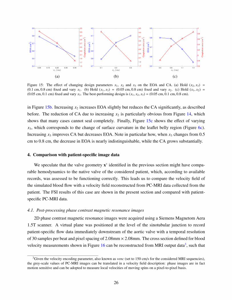
Figure 15: The effect of changing design parameters x1, x2 and x3 on the EOA and CA. (a) Hold (x2, x3) =

(0.1 cm, 0.8 cm) fixed and vary x1. (b) Hold (x1, x3) = (0.05 cm, 0.8 cm) fixed and vary x2. (c) Hold (x1, x2) =

(0.05 cm, 0.1 cm) fixed and vary x3. The best-performing design is (x1, x2, x3) = (0.05 cm, 0.1 cm, 0.8 cm).

in Figure 15b. Increasing x2 increases EOA slightly but reduces the CA significantly, as describedbefore. The reduction of CA due to increasing x2 is particularly obvious from Figure 14, whichshows that many cases cannot seal completely. Finally, Figure 15c shows the effect of varyingx3, which corresponds to the change of surface curvature in the leaflet belly region (Figure 6c).Increasing x3 improves CA but decreases EOA. Note in particular how, when x3 changes from 0.5cm to 0.8 cm, the decrease in EOA is nearly indistinguishable, while the CA grows substantially.

4. Comparison with patient-specific image data

We speculate that the valve geometry x∗ identified in the previous section might have compa-rable hemodynamics to the native valve of the considered patient, which, according to availablerecords, was assessed to be functioning correctly. This leads us to compare the velocity field ofthe simulated blood flow with a velocity field reconstructed from PC-MRI data collected from thepatient. The FSI results of this case are shown in the present section and compared with patient-specific PC-MRI data.

4.1. Post-processing phase contrast magnetic resonance images

2D phase contrast magnetic resonance images were acquired using a Siemens Magnetom Aera1.5T scanner. A virtual plane was positioned at the level of the sinotubular junction to recordpatient-specific flow data immediately downstream of the aortic valve with a temporal resolutionof 30 samples per beat and pixel spacing of 2.08mm × 2.08mm. The cross section defined for bloodvelocity measurements shown in Figure 16 can be reconstructed from MRI output data3, such that

3Given the velocity encoding parameter, also known as venc (set to 150 cm/s for the considered MRI sequencies),the grey-scale values of PC-MRI images can be translated in a velocity field description: phase images are in factmotion sensitive and can be adopted to measure local velocities of moving spins on a pixel-to-pixel basis.

26

Figure 16: Location of the cross section in the medical image data and in the simulation: (a) Long-axis view from MRIhighlighting the cross section considered for phase-contrast blood velocity registration; (b) PC-MRI taken at peak-systole. The green circle highlights the ascending aorta cross section. Grey levels are associated to velocity values. (c)Cross section in the computational model taken consistent with that considered for in-vivo velocity registration.

the simulation results can be plotted and visualized exactly at the same level. We observed fromdynamic MRI records that the identified cross section experiences negligible translation along theaortic centerline (i.e., towards or away from the heart), making the comparison with our fixed-planemeasurements from the numerical simulations fair.

Figure 17 shows the comparison between the velocity field recorded using PC-MRI sequencies(right) and velocity results obtained from the immersogeometric simulation (left) for nine timepoints during the cardiac cycle. From a qualitative point of view, good agreement is observed: flowpatterns of the measured and computed velocity fields are comparable. This tentatively suggeststhat, throughout the entire heart cycle, the developed simulation tool is able to provide hemody-namics predictions sufficiently accurate for medical applications. That is, it is capable of determin-ing local flow profiles which can be associated to parameters of medical interest (e.g., blood flowalterations in case of cardiovascular disease, development of atherosclerosis [95], impairment ofendothelial cells [96], and plaque or aneurysm formation [97, 98]). Differences between measureddata and simulation results can be attributed to a combination of modeling assumptions (e.g., as-sumed pressure profile, simplified aortic wall material model, etc.) and measurement errors (e.g.,limited PC-MRI spatial-temporal resolution, poor signal-to-noise ratio, and difficulty of accuratelysegmenting the moving vessel lumen to extract the blood flow velocities).

Finally, Figure 18 shows several snapshots of the valve deformation and the details of the flowfield at several points during the cardiac cycle. The color indicates the fluid velocity magnitude.The visualization of flows and structures clearly shows the instant response of the valve to theleft ventricular pressure. The valve opens with the rising left ventricular pressure at the beginningstage of systole (0.0–0.09 s), and then stays fully open near the peak systole (0.25 s), allowingsufficient blood flow to enter the ascending aorta. A very quick valve closure is then observedat the beginning of diastole (0.34–0.38 s). This quick closure of the valve minimizes the reverse

27

(a) t = 0.0 s (b) t = 0.045 s (c) t = 0.125 s

(d) t = 0.22 s (e) t = 0.32 s (f) t = 0.34 s

(g) t = 0.35 s (h) t = 0.67 s (i) t = 0.73 s

Figure 17: Comparison between FSI results (left) and patient-specific medical image data (right). The time t issynchronized with Figure 11 for the current cycle. Velocity magnitude is plotted using a color scale ranging from -30cm/s (blue) to 120 cm/s (magenta) for the medical data and from −50 cm/s (blue) to 200 cm/s (magenta) for our FSIresults. The time instant of the medical image is adjusted to match that of our FSI simulation.

flow into the left ventricle as the left ventricular pressure drops rapidly in this period. After that,the valve properly seals and the flow reaches a near-hydrostatic state with no reverse flow (0.55–0.78 s). These flow and structural features during the cardiac cycle characterize a well functioningvalve within the objectives considered in this paper: a large EOA during systole and a proper CAduring diastole. In Figure 19, the models are superposed in the configurations corresponding tothe fully-open and fully-closed phases for better visualization of the leaflet–wall coupling results.The deformation of the attachment edges can be clearly seen. The expansion and contraction ofthe arterial wall as well as its sliding motion between systole and diastole can also be observed.

5. Conclusions

This paper describes a framework for patient-specific design of aortic heart valve replacements.The framework is distinguished by its use of computational FSI models, derived from medicalimaging data from patients, to predict the performance of different heart valve designs in conjunc-tion with an individual patient’s aortic root geometry. The use of such predictive methods has thepotential to reduce patient–prosthesis mismatch.

In the present study, we have limited exploration of the prosthetic valve design space to apredetermined set of designs selected by the analyst. Such an approach is likely sufficient for use

28

Figure 18: Volume rendering visualization of the velocity field from our FSI simulation at several points during acardiac cycle. The time t is synchronized with Figure 11 for the current cycle.

(a) Side view (b) Top view

Figure 19: Relative displacement between fully-open (red) and fully-closed (blue) configurations, showing the effectof leaflet–wall coupling. The deformation of the attachment edges can be clearly seen. The expansion and contractionof the arterial wall as well as its sliding motion between systole (red) and diastole (blue) can also be observed.

with present-day replacement valve technologies. Currently, clinicians have only a finite numberof valves to choose from for each patient. However, in the direction of personalized medicineand looking forward to emerging technologies such as 3D bioprinting, we anticipate that future

29

replacement valve geometries could be optimized and fabricated on a per-patient basis, and webelieve that computational FSI models provide a rational basis for identifying optimal designs.

Extending the design space exploration to the full space of possible valve geometries willrequire some form of automated optimization. We have previously optimized FSI systems using thesurrogate management framework [36], which minimizes a single objective function. In the caseof heart valve design, various objectives pose competing demands on the design, as we discussedin Section 3. This setting necessitates either the careful construction of a quantity of interestthat balances the competing demands, or the use of techniques from multi-objective optimizationto obtain a frontier of Pareto optimal designs. In future work, we plan to extend the frameworkpresented in this paper to include automatic exploration of the design space, to locate optimal valvedesigns without manual selection of candidates and inspection of results by the analyst.

Acknowledgments

This work was supported by the National Heart, Lung, and Blood Institute of the NationalInstitutes of Health under award number R01HL129077. We thank the Texas Advanced Comput-ing Center (TACC) at The University of Texas at Austin for providing HPC resources that havecontributed to the research results reported in this paper. S. Morganti and A. Reali were partiallysupported by the Cariplo/Regione Lombardia iCardioCloud project no. 2013-1779. This supportis gratefully acknowledged. The authors also acknowledge Dr. Francesco Secchi of IRCCS Poli-clinico San Donato for providing medical images, and Sean A. Wasion for his initial work on thisresearch.

References

[1] Taylor CA, Hughes TJR, Zarins CK. Finite element modeling of three-dimensional pulsatileflow in the abdominal aorta: relevance to atherosclerosis. Annals of Biomedical Mngineering

1998; 158:975–987.

[2] Taylor CA, Hughes TJR, Zarins CK. Finite element modeling of blood flow in arteries. Com-

puter Methods in Applied Mechanics and Engineering 1998; 158:155–196.

[3] Taylor CA, Fonte TA, Min JK. Computational fluid dynamics applied to cardiac computedtomography for noninvasive quantification of fractional flow reserve. Journal of the American

College of Cardiology 2013; 61(22):2233–2241.

[4] Zarins CK, Taylor CA, Min JK. Computed fractional flow reserve (FFTCT) derived from coro-nary CT angiography. Journal of Cardiovascular Translational Research 2013; 6(5):708–714.

30

[5] Taylor CA, Draney MT, Ku JP, Parker D, Steele BN, Wang K, Zarins CK. Predic-tive medicine: Computational techniques in therapeutic decision-making. Computer Aided

Surgery 1999; 4(5):231–247.

[6] de Zelicourt DA, Pekkan K, Parks J, Kanter K, Fogel M, Yoganathan AP. Flow study of anextracardiac connection with persistent left superior vena cava. The Journal of Thoracic and

Cardiovascular Surgery 2006; 131(4):785–791.

[7] Pekkan K, Whited B, Kanter K, Sharma S, de Zelicourt D, Sundareswaran K, Frakes D,Rossignac J, Yoganathan AP. Patient-specific surgical planning and hemodynamic com-putational fluid dynamics optimization through free-form haptic anatomy editing tool(SURGEM). Medical & Biological Engineering & Computing 2008; 46(11):1139–1152.

[8] Marsden AL, Bernstein AJ, Reddy VM, Shadden SC, Spilker RL, Chan FP, Taylor CA, Fein-stein JA. Evaluation of a novel Y-shaped extracardiac Fontan baffle using computational fluiddynamics. The Journal of Thoracic and Cardiovascular Surgery 2009; 137(2):394–403.

[9] Neal ML, Kerckhoffs R. Current progress in patient-specific modeling. Briefings in Bioinfor-

matics 2010; 11(1):111–126.

[10] Sankaran S, Moghadam ME, Kahn AM, Tseng EE, Guccione JM, Marsden AL. Patient-specific multiscale modeling of blood flow for coronary artery bypass graft surgery. Annals

of Biomedical Engineering 2012; 40(10):2228–2242.

[11] Morganti S, Conti M, Aiello M, Valentini A, Mazzola A, Reali A, Auricchio F. Simulation oftranscatheter aortic valve implantation through patient-specific finite element analysis: Twoclinical cases. Journal of Biomechanics 2014; 47(11):2547–2555.

[12] Morganti S, Brambilla N, Petronio AS, Reali A, Bedogni F, Auricchio F. Prediction of patient-specific post-operative outcomes of TAVI procedure: The impact of the positioning strategyon valve performance. Journal of Biomechanics 2016; 49(12):2513–2519.

[13] Zarins CK, Taylor CA. Endovascular device design in the future: Transformation from trialand error to computational design. Journal of Endovascular Therapy 2009; 16:I12–I21.

[14] Marsden AL, Reddy VM, Shadden SC, Chan FP, Taylor CA, Feinstein JA. A new multipa-rameter approach to computational simulation for Fontan assessment and redesign. Congen-

ital Heart Disease 2010; 5(2):104–117.

[15] Auricchio F, Conti M, Morganti S, Totaro P. A computational tool to support pre-operative planning of stentless aortic valve implant. Medical Engineering & Physics 2011;33(10):1183–1192.

31

[16] Long CC, Marsden AL, Bazilevs Y. Shape optimization of pulsatile ventricular assist devicesusing FSI to minimize thrombotic risk. Computational Mechanics 2014; 54(4):921–932.

[17] Fan R, Bayoumi AS, Chen P, Hobson CM, Wagner WR, Mayer Jr JE, Sacks MS. Optimalelastomeric scaffold leaflet shape for pulmonary heart valve leaflet replacement. Journal of

Biomechanics 2013; 46(4):662–669.

[18] Pibarot P, Dumesnil JG. Prosthetic heart valves. Circulation 2009; 119(7):1034–1048.

[19] Otto CM. Timing of aortic valve surgery. Heart 2000; 84(2):211–218.

[20] Thubrikar MJ, Deck JD, Aouad J, Nolan SP. Role of mechanical stress in calcificationof aortic bioprosthetic valves. The Journal of Thoracic and Cardiovascular Surgery 1983;86(1):115–125.

[21] Sun W, Abad A, Sacks MS. Simulated bioprosthetic heart valve deformation under quasi-static loading. Journal of Biomechanical Engineering 2005; 127(6):905–914.

[22] Kim H, Lu J, Sacks MS, Chandran KB. Dynamic simulation pericardial bioprosthetic heartvalve function. Journal of Biomechanical Engineering 2006; 128(5):717–724.

[23] Marom G. Numerical methods for fluid–structure interaction models of aortic valves.Archives of Computational Methods in Engineering 2014; 22(4):595–620.

[24] Vesely I. The evolution of bioprosthetic heart valve design and its impact on durability. Car-

diovascular Pathology 2003; 12(5):277–286.

[25] Xiong FL, Goetz WA, Chong CK, Chua YL, Pfeifer S, Wintermantel E, Yeo JH. Finite ele-ment investigation of stentless pericardial aortic valves: relevance of leaflet geometry. Annals

of Biomedical Engineering 2010; 38(5):1908–1918.

[26] Ennker J, Albert A, Ennker IC. Stentless aortic valves. Current aspects. HSR Proc Intensive

Care Cardiovasc Anesth 2012; 4(2):77–82.

[27] David TE. Aortic valve sparing operations: a review. The Korean Journal of Thoracic and

Cardiovascular Surgery 2012; 45(4):205–212.

[28] Grbic S, Ionasec R, Vitanovski D, Voigt I, Wang Y, Georgescu B, Navab N, Comaniciu D.Complete valvular heart apparatus model from 4D cardiac CT. Medical Image Analysis 2012;16(5):1003–1014.

[29] Mansi T, Houle H, Voigt I, Szucs M, Hunter E, Datta S, Comaniciu D. Quantifying heartvalves: From diagnostic to personalized valve repair 2016. Siemens White Paper.

32

[30] Hughes TJR, Cottrell JA, Bazilevs Y. Isogeometric analysis: CAD, finite elements, NURBS,exact geometry, and mesh refinement. Computer Methods in Applied Mechanics and Engi-

neering 2005; 194:4135–4195.

[31] Morganti S, Auricchio F, Benson DJ, Gambarin FI, Hartmann S, Hughes TJR, Reali A.Patient-specific isogeometric structural analysis of aortic valve closure. Computer Methods

in Applied Mechanics and Engineering 2015; 284:508–520.

[32] Sotiropoulos F, Yang X. Immersed boundary methods for simulating fluid–structure interac-tion. Progress in Aerospace Sciences 2014; 65:1–21.

[33] Kamensky D, Hsu MC, Schillinger D, Evans JA, Aggarwal A, Bazilevs Y, Sacks MS, HughesTJR. An immersogeometric variational framework for fluid–structure interaction: applica-tion to bioprosthetic heart valves. Computer Methods in Applied Mechanics and Engineering

2015; 284:1005–1053.

[34] Hsu MC, Wang C, Xu F, Herrema AJ, Krishnamurthy A. Direct immersogeometric fluid flowanalysis using B-rep CAD models. Computer Aided Geometric Design 2016; 43:143–158.

[35] Wang C, Xu F, Hsu MC, Krishnamurthy A. Rapid B-rep model preprocessing for immer-sogeometric analysis using analytic surfaces. Computer Aided Geometric Design 2017; 52–53:190–204.

[36] Wu MCH, Kamensky D, Wang C, Herrema AJ, Xu F, Pigazzini MS, Verma A, Marsden AL,Bazilevs Y, Hsu MC. Optimizing fluid–structure interaction systems with immersogeometricanalysis and surrogate modeling: Application to a hydraulic arresting gear. Computer Meth-

ods in Applied Mechanics and Engineering 2017; 316:668–693.

[37] Hsu MC, Kamensky D, Xu F, Kiendl J, Wang C, Wu MCH, Mineroff J, Reali A, Bazilevs Y,Sacks MS. Dynamic and fluid–structure interaction simulations of bioprosthetic heart valvesusing parametric design with T-splines and Fung–type material models. Computational Me-

chanics 2015; 55:1211–1225.

[38] Thubrikar M. The Aortic Valve. CRC Press, Inc.: Boca Raton, Florida, 1990.

[39] Labrosse MR, Beller CJ, Robicsek F, Thubrikar MJ. Geometric modeling of functionaltrileaflet aortic valves: Development and clinical applications. Journal of Biomechanics 2006;39(14):2665–2672.

[40] Haj-Ali R, Marom G, Zekry SB, Rosenfeld M, Raanani E. A general three-dimensional para-metric geometry of the native aortic valve and root for biomechanical modeling. Journal of

Biomechanics 2012; 45(14):2392–2397.

33

[41] Kouhi E, Morsi YS. A parametric study on mathematical formulation and geometrical con-struction of a stentless aortic heart valve. Journal of Artificial Organs 2013; 16(4):425–442.

[42] Li K, Sun W. Simulated transcatheter aortic valve deformation: A parametric study on theimpact of leaflet geometry on valve peak stress. International Journal for Numerical Methods

in Biomedical Engineering 2017; 33(3):e02 814.

[43] Murphy SV, Atala A. 3D bioprinting of tissues and organs. Nature Biotechnology 2014;32(8):773–785.

[44] Duan B, Hockaday LA, Kang KH, Butcher JT. 3D bioprinting of heterogeneous aortic valveconduits with alginate/gelatin hydrogels. Journal of Biomedical Materials Research Part A

2013; 101(5):1255–1264.

[45] Votta E, Le TB, Stevanella M, Fusini L, Caiani EG, Redaelli A, Sotiropoulos F. Towardpatient-specific simulations of cardiac valves: state-of-the-art and future directions. Journal

of Biomechanics 2013; 46(2):217–228.

[46] The Vascular Modeling Toolkit. http://www.vmtk.org/. Accessed 1 May 2017.

[47] Antiga L, Piccinelli M, Botti L, Ene-Iordache B, Remuzzi A, Steinman DA. An image-basedmodeling framework for patient-specific computational hemodynamics. Medical & Biologi-

cal Engineering & Computing 2008; 46(11):1097–1112.

[48] Turkbey EB, Jain A, Johnson C, Redheuil A, Arai AE, Gomes AS, Carr J, Hundley WG,Teixido-Tura G, Eng J, et al.. Determinants and normal values of ascending aortic diameterby age, gender, and race/ethnicity in the Multi-Ethnic Study of Atherosclerosis (MESA).Journal of Magnetic Resonance Imaging 2014; 39(2):360–368.

[49] Tezduyar T, Aliabadi S, Behr M, Johnson A, Mittal S. Parallel finite-element computation of3D flows. Computer 1993; 26(10):27–36.

[50] Johnson AA, Tezduyar TE. Mesh update strategies in parallel finite element computations offlow problems with moving boundaries and interfaces. Computer Methods in Applied Me-

chanics and Engineering 1994; 119:73–94.

[51] Bazilevs Y, Calo VM, Hughes TJR, Zhang Y. Isogeometric fluid–structure interaction: theory,algorithms, and computations. Computational Mechanics 2008; 43:3–37.

[52] Toshniwal D, Speleers H, Hiemstra RR, Hughes TJ. Multi-degree smooth polar splines: Aframework for geometric modeling and isogeometric analysis. Computer Methods in Applied

Mechanics and Engineering 2017; 316:1005–1061.

34

[53] Stein K, Tezduyar T, Benney R. Mesh moving techniques for fluid–structure interactions withlarge displacements. Journal of Applied Mechanics 2003; 70:58–63.

[54] Hsu MC, Wang C, Herrema AJ, Schillinger D, Ghoshal A, Bazilevs Y. An interactive ge-ometry modeling and parametric design platform for isogeometric analysis. Computers and

Mathematics with Applications 2015; 70:1481–1500.

[55] Rhinoceros. http://www.rhino3d.com/. Accessed 1 May 2017.

[56] Grasshopper. http://www.grasshopper3d.com/. Accessed 1 May 2017.

[57] Bazilevs Y, Hsu MC, Scott MA. Isogeometric fluid–structure interaction analysis with em-phasis on non-matching discretizations, and with application to wind turbines. Computer

Methods in Applied Mechanics and Engineering 2012; 249–252:28–41.

[58] Simo JC, Hughes TJR. Computational Inelasticity. Springer-Verlag: New York, 1998.

[59] Lipton S, Evans JA, Bazilevs Y, Elguedj T, Hughes TJR. Robustness of isogeometric struc-tural discretizations under severe mesh distortion. Computer Methods in Applied Mechanics

and Engineering 2010; 199:357–373.

[60] Bazilevs Y, Hsu MC, Zhang Y, Wang W, Kvamsdal T, Hentschel S, Isaksen J. Computationalfluid–structure interaction: Methods and application to cerebral aneurysms. Biomechanics

and Modeling in Mechanobiology 2010; 9:481–498.

[61] Hsu MC, Bazilevs Y. Blood vessel tissue prestress modeling for vascular fluid–structure in-teraction simulations. Finite Elements in Analysis and Design 2011; 47:593–599.

[62] Kiendl J, Bletzinger KU, Linhard J, Wuchner R. Isogeometric shell analysis with Kirchhoff–Love elements. Computer Methods in Applied Mechanics and Engineering 2009; 198:3902–3914.

[63] Kiendl J, Bazilevs Y, Hsu MC, Wuchner R, Bletzinger KU. The bending strip method for iso-geometric analysis of Kirchhoff–Love shell structures comprised of multiple patches. Com-

puter Methods in Applied Mechanics and Engineering 2010; 199:2403–2416.

[64] Kiendl J, Hsu MC, Wu MCH, Reali A. Isogeometric Kirchhoff–Love shell formulations forgeneral hyperelastic materials. Computer Methods in Applied Mechanics and Engineering

2015; 291:280–303.

[65] Hillairet M. Lack of collision between solid bodies in a 2D incompressible viscous flow.Communications in Partial Differential Equations 2007; 32(9):1345–1371.

35

[66] Rukmani R, Usha R. Arbitrary squeeze flow between two disks. International Journal of

Mathematics and Mathematical Sciences 1994; 17:779–782.

[67] Hughes TJR, Liu WK, Zimmermann TK. Lagrangian–Eulerian finite element formulationfor incompressible viscous flows. Computer Methods in Applied Mechanics and Engineering

1981; 29:329–349.

[68] Hughes TJR, Wells GN. Conservation properties for the Galerkin and stabilised forms ofthe advection–diffusion and incompressible Navier–Stokes equations. Computer Methods in

Applied Mechanics and Engineering 2005; 194:1141–1159.

[69] Brooks AN, Hughes TJR. Streamline upwind/Petrov-Galerkin formulations for convectiondominated flows with particular emphasis on the incompressible Navier–Stokes equations.Computer Methods in Applied Mechanics and Engineering 1982; 32:199–259.

[70] Tezduyar TE. Stabilized finite element formulations for incompressible flow computations.Advances in Applied Mechanics 1992; 28:1–44.

[71] Hughes TJR, Mazzei L, Jansen KE. Large eddy simulation and the variational multiscalemethod. Computing and Visualization in Science 2000; 3:47–59.

[72] Hughes TJR, Mazzei L, Oberai AA, Wray A. The multiscale formulation of large eddy sim-ulation: Decay of homogeneous isotropic turbulence. Physics of Fluids 2001; 13:505–512.

[73] Bazilevs Y, Calo VM, Cottrel JA, Hughes TJR, Reali A, Scovazzi G. Variational multiscaleresidual-based turbulence modeling for large eddy simulation of incompressible flows. Com-

puter Methods in Applied Mechanics and Engineering 2007; 197:173–201.

[74] Hsu MC, Bazilevs Y, Calo VM, Tezduyar TE, Hughes TJR. Improving stability of stabilizedand multiscale formulations in flow simulations at small time steps. Computer Methods in

Applied Mechanics and Engineering 2010; 199:828–840.

[75] Chung J, Hulbert GM. A time integration algorithm for structural dynamics with improvednumerical dissipation: The generalized-α method. Journal of Applied Mechanics 1993;60:371–75.

[76] Simo JC, Wriggers P, Taylor RL. A perturbed Lagrangian formulation for the finite elementsolution of contact problems. Computer Methods in Applied Mechanics and Engineering

1985; 50(2):163–180.

36

[77] Kamensky D, Evans JA, Hsu MC. Stability and conservation properties of collocated con-straints in immersogeometric fluid-thin structure interaction analysis. Communications in

Computational Physics 2015; 18:1147–1180.

[78] Kamensky D, Hsu MC, Yu Y, Evans JA, Sacks MS, Hughes TJ. Immersogeometric cardiovas-cular fluid–structure interaction analysis with divergence-conforming B-splines. Computer

Methods in Applied Mechanics and Engineering 2017; 314:408–472.

[79] Soares JS, Feaver KR, Zhang W, Kamensky D, Aggarwal A, Sacks MS. Biomechanical be-havior of bioprosthetic heart valve heterograft tissues: Characterization, simulation, and per-formance. Cardiovascular Engineering and Technology 2016; 7(4):309–351.

[80] Garcia D, Kadem L. What do you mean by aortic valve area: geometric orifice area, effectiveorifice area, or Gorlin area? Journal of Heart Valve Disease 2006; 15(5):601.

[81] Gorlin R, Gorlin SG. Hydraulic formula for calculation of the area of the stenotic mitralvalve, other cardiac valves, and central circulatory shunts. I. American Heart Journal 1951;41(1):1–29.

[82] Cannon SR, Richards KL, Crawford M. Hydraulic estimation of stenotic orifice area: a cor-rection of the Gorlin formula. Circulation 1985; 71(6):1170–1178.

[83] Skjaerpe T, Hegrenaes L, Hatle L. Noninvasive estimation of valve area in patients with aorticstenosis by Doppler ultrasound and two-dimensional echocardiography. Circulation 1985;72(4):810–818.

[84] Otto CM, Pearlman AS, Comess KA, Reamer RP, Janko CL, Huntsman LL. Determinationof the stenotic aortic valve area in adults using Doppler echocardiography. Journal of the

American College of Cardiology 1986; 7(3):509–517.

[85] Garcia D, Dumesnil JG, Durand LG, Kadem L, Pibarot P. Discrepancies between catheter andDoppler estimates of valve effective orifice area can be predicted from the pressure recoveryphenomenon: practical implications with regard to quantification of aortic stenosis severity.Journal of the American College of Cardiology 2003; 41(3):435–442.

[86] le Polain de Waroux JB, Pouleur AC, Robert A, Pasquet A, Gerber BL, Noirhomme P,El Khoury G, Vanoverschelde JLJ. Mechanisms of recurrent aortic regurgitation after aor-tic valve repair. JACC: Cardiovascular Imaging 2009; 2(8):931–939.

[87] Chandran KB, Kim SH, Han G. Stress distribution on the cusps of a polyurethane trileafletheart valve prosthesis in the closed position. Journal of Biomechanics 1991; 24(6):389–395.

37

[88] Grande KJ, Cochran RP, Reinhall PG, Kunzelman KS. Stress variations in the human aorticroot and valve: the role of anatomic asymmetry. Annals of Biomedical Engineering 1998;26(4):534–545.

[89] Harringer W, Pethig K, Hagl C, Meyer GP, Haverich A. Ascending aortic replacement withaortic valve reimplantation. Circulation 1999; 100(suppl II):II24–II28.

[90] Kim H, Lu J, Sacks MS, Chandran KB. Dynamic simulation of bioprosthetic heart valvesusing a stress resultant shell model. Annals of Biomedical Engineering 2008; 36(2):262–275.

[91] Marom G, Haj-Ali R, Raanani E, Schafers HJ, Rosenfeld M. A fluid–structure interactionmodel of the aortic valve with coaptation and compliant aortic root. Medical & Biological

Engineering & Computing 2012; 50:173–182.

[92] Takizawa K, Bazilevs Y, Tezduyar TE. Space–time and ALE-VMS techniques for patient-specific cardiovascular fluid–structure interaction modeling. Archives of Computational

Methods in Engineering 2012; 19:171–225.

[93] Vignon-Clementel IE, Figueroa CA, Jansen KE, Taylor CA. Outflow boundary conditions forthree-dimensional finite element modeling of blood flow and pressure in arteries. Computer

Methods in Applied Mechanics and Engineering 2006; 195:3776–3796.

[94] Yap CH, Saikrishnan N, Tamilselvan G, Yoganathan AP. Experimental technique of mea-suring dynamic fluid shear stress on the aortic surface of the aortic valve leaflet. Journal of

Biomechanical Engineering 2011; 133(6):061 007.

[95] Cheng C, Tempel D, van Haperen R, van der Baan A, Grosveld F, Daemen M, Krams R,de Crom R. Atherosclerotic lesion size and vulnerability are determined by patterns of fluidshear stress. Circulation 2006; 113:2744–2753.

[96] Chien S, Li S, Shyy Y. Effects of mechanical forces on signal transduction and gene expres-sion in endothelial cells. Hypertension 1998; 313:162–169.

[97] Wentzel JJ, Corti R, Fayad ZA, Wisdom P, Macaluso F, Winkelman MO, Fuster V, BadimonJJ. Does shear stress modulate both plaque progression and regression in the thoracic aorta?Human study using serial magnetic resonance imaging. Journal of the American College of

Cardiology 2005; 45:846–854.

[98] Shojima M, Oshima M, Takagi K, Torii R, Hayakawa M, Katada K, Morita A, Kirino T.Magnitude and role of wall shear stress on cerebral aneurysm: computational fluid dynamicstudy of 20 middle cerebral artery aneurysms. Stroke 2004; 35:2500–2505.

38