ias0031 modeling and identification lecture 2: linear
TRANSCRIPT

IAS0031 Modeling and Identification
Lecture 2: Linear Programming. Optimiza-tion. Convexity. Practical Optimization.
Aleksei Tepljakov, Ph.D.

Part I: Linear Programming
Aleksei Tepljakov 2 / 39

Phone Dealer Example
Aleksei Tepljakov 3 / 39
A phone dealer goes to the wholesale market with 1500EUR topurchase phones for selling. There are different types of phonesavailable on the market, but having compared technicalspecifications of all available phones, he decides that there are twophone types, P1 and P2 that would be suitable for resale in hisregion of interest. The first type of phone (P1) would cost thedealer 300EUR and the second type of phone (P2)—250EUR.
However, the dealer knows that he can sell the P1 phone for325EUR, and P2 phone for 265EUR. With the available amount ofmoney he would like to make maximum profit. His problem is tofind out how many phones of each type should be purchased to getmaximum profit, assuming he would succesfully market and sell allof the acquired phones later.

Phone Dealer Example: Solution
Aleksei Tepljakov 4 / 39
The problem is formulated as
z = 325P1 + 265P2 → max
under the constraint 300P1 + 250P2 6 1500 and bounds P1, P2 > 0. Solution:
P1 P2 Investment Amount after sale Profit
0 6 1500 1590 90
1 4 1300 1385 85
2 3 1350 1445 95
3 2 1400 1505 105
4 1 1450 1565 115
5 0 1500 1625 125

Linear Programming: Basic Definitions
Aleksei Tepljakov 5 / 39
Definition 1. The function to be maximized
z = f(x1, x2, . . . , xn) → max
or minimized
z = f(x1, x2, . . . , xn) → min
is called the objective function.
Definition 2. The limitations on resources which are to be
allocated among various competing variables in form of equations
or inequalities and are called constraints or restrictions.
Definition 3. Constraints on individual variables in form of
inequalities are called bounds.
Linear Programming: Basic Definitions(continued)
Aleksei Tepljakov 6 / 39
Definition 4. A linear programming problem may be defined as
the problem of maximizing or minimizing a linear function subject
to linear constraints.
Definition 5. A vector x for the optimization problem is said to be
feasible if it satises all the constraints.
Definition 6. A vector x is optimal if it feasible and optimizes the
objective function over feasible x.
Definition 7. A linear programming problem is said to be feasible
if there exist a feasible vector x for it; otherwise, it is said to be
infeasible.
The Standard Maximum Problem
Aleksei Tepljakov 7 / 39
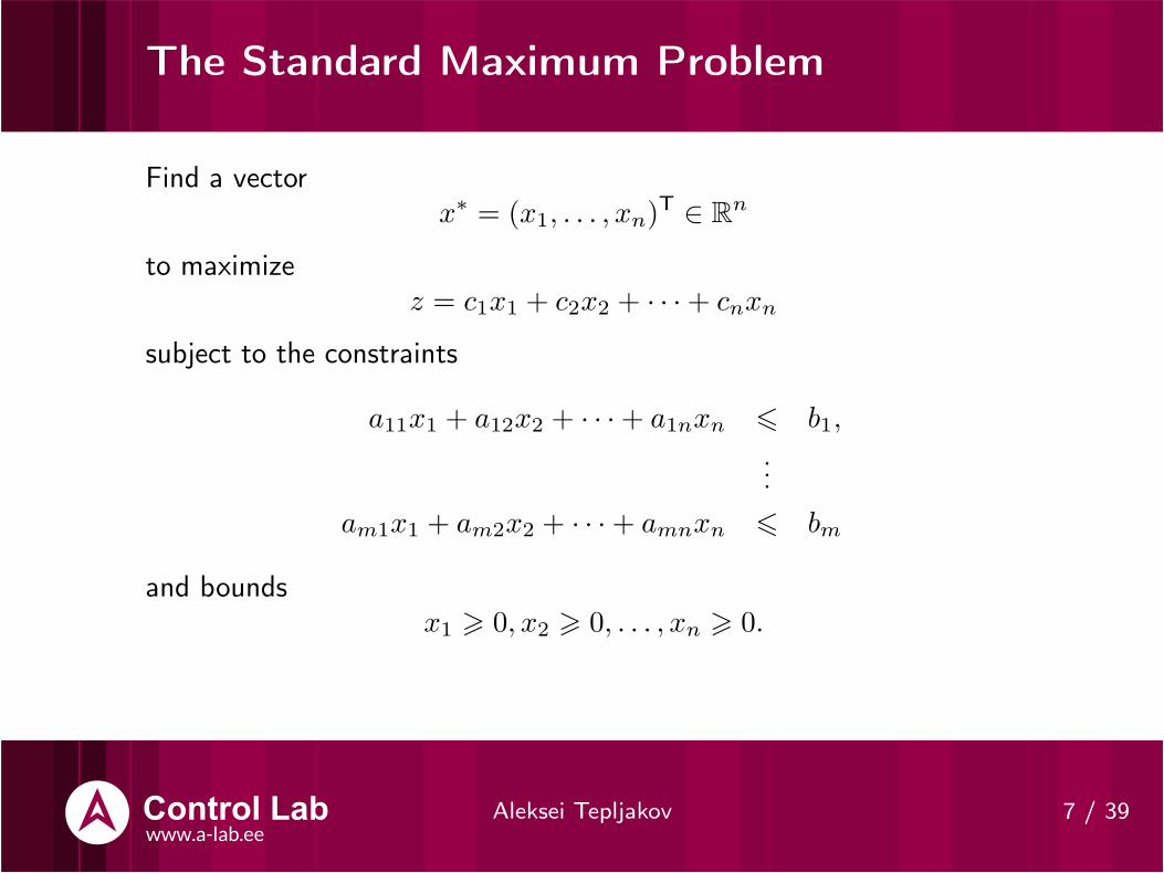
Find a vectorx∗ = (x1, . . . , xn)
T ∈ Rn
to maximizez = c1x1 + c2x2 + · · ·+ cnxn
subject to the constraints
a11x1 + a12x2 + · · ·+ a1nxn 6 b1,
...
am1x1 + am2x2 + · · ·+ amnxn 6 bm
and boundsx1 > 0, x2 > 0, . . . , xn > 0.

Matrix Form of the Linear ProgrammingProblem
Aleksei Tepljakov 8 / 39
Suppose that
X =
x1
x2
...xn
, A =
a11 a12 · · · a1na21 a22 · · · a2n...
.... . .
...am1 am2 · · · amn
, B =
b1b2...bm
, C =
c1c2...cn
T
,
then the linear programming problem can be rewritten:
z = CX → max(min)AX 6 BX > 0
(standard form)
orz = CX → max(min)
AX = BX > 0
(canonical form)

Formulation and Solution of a LinearProgramming Problem
Aleksei Tepljakov 9 / 39
Formulation:
• Identify the decision variables to be determined and express them in termsof algebraic symbols, e.g., x1, x2, . . . , xn;
• Identify the objective which is to be optimized (maximized or minimized)and express it as a linear function of the above defined decision variables;
• Identify all the limitations in the given problem and then express them aslinear equations or inequalities in terms of above defined decision variables.
Some solution methods:
• Graphical method;
• Analytical method or trial and error method;
• Simplex method.

Common Linear Programming Problems:Production Planning Problem
Aleksei Tepljakov 10 / 39
A company manufactures two types of products—P1 and P2—andsells them at a profit of 2EUR and 3EUR, respectively. Eachproduct is processed on two machines M1 and M2. P1 requires 1minute of processing time on M1 and 2 minutes on M2, type P2
requires 1 minute on M1 and 1 minute on M2. The machine M1 isavailable for not more than 6 hours and 40 minutes, while machineM2 is available for 10 hours during one working day. The problemis to maximize the profit of the company.

Common Linear Programming Problems:Production Planning Problem (continued)
Aleksei Tepljakov 11 / 39
Arrange the data in form of a table
MachineProcessing time
Available timeP1 P2
M1 1 1 400M2 2 1 600
Profit 2 3
And formulate the problem
z = 2x1 + 3x2 → max
x1 + x2 6 400
2x1 + x2 6 600
with x1 > 0, x2 > 0.

Common Linear Programming Problems:The Diet Problem
Aleksei Tepljakov 12 / 39
Let there be three different types of food—F1, F2, F3—that supply varyingquantities of 2 nutrients—N1 and N2—that are essential to good health.Suppose a person has decided to make an individual plan to improve thehealth. We know that 400g and 1kg are the minimum daily requirements ofnutrients N1 and N2, respectively. Moreover, the corresponding unit of foodF1, F2, F3 costs 2, 4, and 3EUR, respectively. Finally, we know that
• one unit of food F1 contains 20g of nutrient N1 and 40g of nutrient N2;
• one unit of food F2 contains 25g of nutrient N1 and 62g of nutrient N2;
• one unit of food F3 contains 30g of nutrient N1 and 75g of nutrient N2.
The problem is to supply the required nutrients at minimum cost.

Common Linear Programming Problems:The Diet Problem (continued)
Aleksei Tepljakov 13 / 39
Arrange the data into a table:
NutrientFood
Daily requirementF1 F2 F3
N1 20 25 30 400N2 40 62 75 1000
Profit 2 4 3
The problem is given by
z = 2x1 + 4x2 + 3x3 → min
20x1 + 25x2 + 30x3 > 400
40x1 + 62x2 + 75x3 > 1000
with x1 > 0, x2 > 0, x3 > 0.

Linear Programming Problem: GeometricApproach
Aleksei Tepljakov 14 / 39
If a linear programming problem can be represented by a system with twovariables, the geometric approach may be used to solve it. It comprises thefollowing steps:
1. Formulate the linear programming problem.
2. Graph the constraints inequalities.
3. Identify the feasible region which satisfies all the constraintssimultaneously.
4. Locate the solution points on the feasible region. These points alwaysoccur at the vertex of the feasible region.
5. Evaluate the objective function at each of the vertex (corner point).
6. Identify the optimum value of the objective function. For a boundedregion, both a minimum and maximum value will exist. For an unboundedregion, if an optimal solution exists, then it will occur at a vertex.

Optimal Solution of a Linear ProgrammingProblem
Aleksei Tepljakov 15 / 39
• If a linear programming problem has a solution, it must occur ata vertex of the set of feasible solutions.
• If the problem has more than one solution, then at least one ofthem must occur at a vertex of the set of feasible solutions.
• If none of the feasible solutions maximizes (or minimizes) theobjective function, or if there are no feasible solutions, then thelinear programming problem has no solutions.

Graphical Method: Example 1
Aleksei Tepljakov 16 / 39
z = x1 + 2x2 → max(min)
x1 + x2 > 1
with x1 > 0, x2 > 0.
Analysis: The vertices of the
feasible region are A(0, 1) and
B(1, 0). The minimum value is
attained at B(1, 0), where
z(1, 0) = 1, since z(0, 1) = 2.
This problem has no solution in case of the problem of maximizingthe objective function, since the feasible region is unbounded.
Graphical Method: Example 2
Aleksei Tepljakov 17 / 39
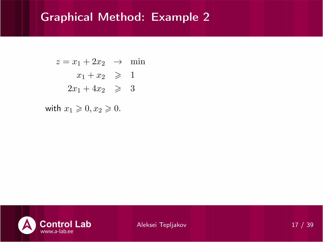
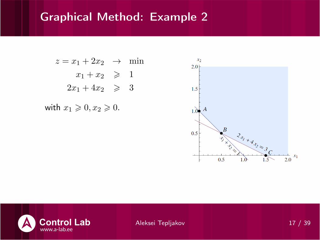
z = x1 + 2x2 → min
x1 + x2 > 1
2x1 + 4x2 > 3
with x1 > 0, x2 > 0.
Analysis: Check the vertices of the
feasible region and find that
z(A) = 2, z(B) = 1.5, and
z(C) = 1.5. The problem has
infinitely many solutions located on
the line segment BC.
Graphical Method: Example 2
Aleksei Tepljakov 17 / 39
z = x1 + 2x2 → min
x1 + x2 > 1
2x1 + 4x2 > 3
with x1 > 0, x2 > 0.
Analysis: Check the vertices of the
feasible region and find that
z(A) = 2, z(B) = 1.5, and
z(C) = 1.5. The problem has
infinitely many solutions located on
the line segment BC.

Graphical Method: Example 2
Aleksei Tepljakov 17 / 39
z = x1 + 2x2 → min
x1 + x2 > 1
2x1 + 4x2 > 3
with x1 > 0, x2 > 0.
Analysis: Check the vertices of the
feasible region and find that
z(A) = 2, z(B) = 1.5, and
z(C) = 1.5. The problem has
infinitely many solutions located on
the line segment BC.

Graphical Method: Example 3
Aleksei Tepljakov 18 / 39
z = 2x1 + x2 → max(min)
x1 + 2x2 6 2
x1 + x2 6 1.5
with x1 > 0, x2 > 0.
Analysis: Check the vertices of the
feasible region z(O) = 0, z(A) = 1,
z(B) = 2.5, and z(C) = 3. The
maximum value of z is obtained at
vertex C(1.5, 0). The minimum
value is obtained at O(0, 0).

Part II: Optimization. Convexity
Aleksei Tepljakov 19 / 39

General Nonlinear Optimization Problem
Aleksei Tepljakov 20 / 39
The single objective optimization problem can be written as
minx∈Rn
f(x) subject to
ci(x) = 0, i ∈ I ,
qj(x) 6 0, j ∈ E ,
λk 6 xk 6 ξk, k ∈ K ,
(1)
where f , ci and qj are scalar-valued functions of the variables x, λk
and ξk are scalar bounds, and I ,E , and K are sets of indices.
The linear programming problem is therefore a particular case ofthe general optimization problem stated above.

Types of Optimization Problems
Aleksei Tepljakov 21 / 39
Based on the search variable set:
• Continuous: Solutions belong to an uncountably infinite set, e.g.,x ∈ R
n;
• Discrete: Solutions belong to a limited set, e.g., x ∈ {1, 2, 3}.Based on constraints:
• Unconstrained : Such problems arise directly in many practicalapplications, where it is safe to disregard certain constraints;
• Constrained : Such problems arise from models that include specificconstraints on the variables, e.g., bounds and nonlinear constraints;
To make a transition from an unconstrained problem to a constrainedone it is also to modify the objective function by adding penalizing terms.

Numerical Optimization Algorithms
Aleksei Tepljakov 22 / 39
Optimization algorithms are iterative processes, which are started by choosingan initial estimate for the solution, and generate a series of improved estimatesuntil a solution is found. The following properties ARE essential to any goodoptimization algorithm:
• Accuracy. The algorithm should be able to identify a solution withadequate precision without being sensitive to errors in the data or torounding errors that occur due to limited computational capacity of theimplementation.
• Robustness. The algorithm should perform well on a wide variety ofproblems for all reasonable choices of the initial estimates.
• Efficiency. The algorithm should not require too much computer time ormemory storage.
These goals usually conflict, especially in case of complex optimizationproblems, so tradeoffs must be sought.

Convexity
Aleksei Tepljakov 23 / 39
Let S 6= ∅, S ⊂ Rn and x1, x2 ∈ S.
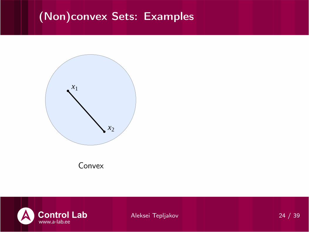
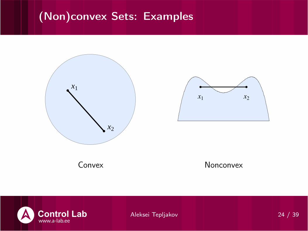
Definition 8. The set [x1, x2] = {x|x = λx1 + (1− λ)x2,0 ≤ λ ≤ 1} is called a line segment with the endpoints x1, x2.
Definition 9. The set S is called a convex set if the line segment
joining any pair of points x1, x2 ∈ S lies entirely in S.
Definition 10. The function f is called convex if its domain D is
a convex set and for any two points x1, x2 ∈ D there holds
f(λx1 + (1− λ)x2) 6 λf(x1) + (1− λ)f(x2), ∀λ ∈ [0, 1]. (2)
(That is: The graph of f lies below the straight line connecting(x1, f(x1)) to (x2, f(x2)).)

Convexity
Aleksei Tepljakov 23 / 39
Let S 6= ∅, S ⊂ Rn and x1, x2 ∈ S.
Definition 8. The set [x1, x2] = {x|x = λx1 + (1− λ)x2,0 ≤ λ ≤ 1} is called a line segment with the endpoints x1, x2.
Definition 9. The set S is called a convex set if the line segment
joining any pair of points x1, x2 ∈ S lies entirely in S.
Definition 10. The function f is called convex if its domain D is
a convex set and for any two points x1, x2 ∈ D there holds
f(λx1 + (1− λ)x2) 6 λf(x1) + (1− λ)f(x2), ∀λ ∈ [0, 1]. (2)
(That is: The graph of f lies below the straight line connecting(x1, f(x1)) to (x2, f(x2)).)

(Non)convex Sets: Examples
Aleksei Tepljakov 24 / 39
x1
x2
Convex Nonconvex
(Non)convex Sets: Examples
Aleksei Tepljakov 24 / 39
x1
x2
Convex
Nonconvex

(Non)convex Sets: Examples
Aleksei Tepljakov 24 / 39
x1
x2
Convex
Nonconvex
(Non)convex Sets: Examples
Aleksei Tepljakov 24 / 39
x1
x2
Convex Nonconvex

(Non)convex Sets: Examples (continued)
Aleksei Tepljakov 25 / 39
x1
x2
Nonconvex
1
2
Convex

(Non)convex Sets: Examples (continued)
Aleksei Tepljakov 25 / 39
x1
x2
Nonconvex
1
2
Convex

(Non)convex Sets: Examples (continued)
Aleksei Tepljakov 25 / 39
x1
x2
Nonconvex
x1
x2
Convex

(Non)convex Sets: Examples (continued)
Aleksei Tepljakov 25 / 39
x1
x2
Nonconvex
x1
x2
Convex

Convex Function: Illustration
Aleksei Tepljakov 26 / 39

Convexity: Some Propositions
Aleksei Tepljakov 27 / 39
Proposition 1. A solution set L for the linear inequality a1x1 + a2x2 +a3x3 + · · ·+ anxn ≤ b is a convex set.
Proposition 2. The intersection of any finite number of convex sets is also aconvex set.
Corollary 1. The solution set of a system of linear equations (inequalities) is aconvex set.
Corollary 2. The solution set of constraints for linear programming problem(set of feasible solutions) is a convex set.
Definition 11. Given a finite number of points x1, x2, . . . , xn in a real vectorspace, a convex combination of these points is a point of the formα1x1 +α2x2 + · · ·+ αnxn, where αi ∈ R, αi ≥ 0 and α1 +α2 + · · ·+αn = 1.
Definition 12. Let x be a convex combination of points from the set S. Then,S is called convex if x ∈ S.

Convex Optimization Problem
Aleksei Tepljakov 28 / 39
Definition 13. A point x∗ is a local minimizer of the function fif there is a neighborhood N of x∗such that f(x∗) 6 f(x) for all
x ∈ N .
Definition 14. A point x∗ is a global minimizer of the function fif f(x∗) 6 f(x) for all x.
Definition 15. A convex optimization problem is a problem where
all of the constraints are convex functions, and the objective is a
convex function.
Theorem 1. When f is convex, any local minimizer x∗ is a global
minimizer of f . If in addition f is differentiable, then any
stationary point x∗ is a global minimizer of f .

Linear Programming as a Special Case ofConvex Optimization Problem
Aleksei Tepljakov 29 / 39
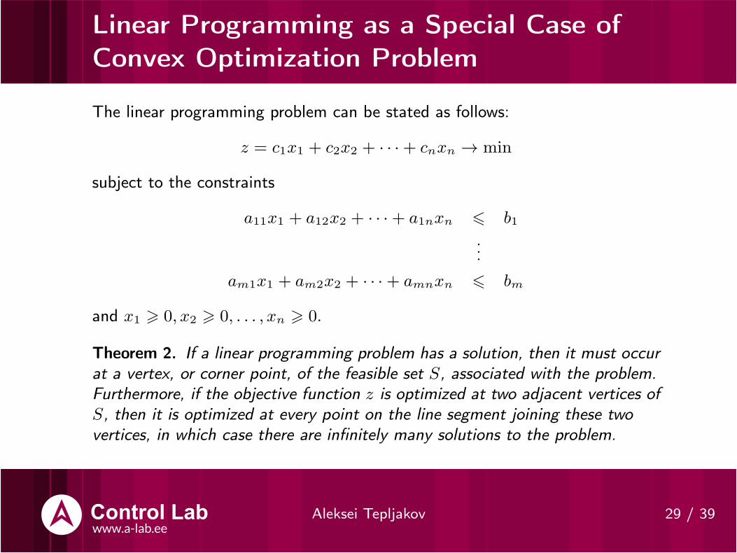
The linear programming problem can be stated as follows:
z = c1x1 + c2x2 + · · ·+ cnxn → min
subject to the constraints
a11x1 + a12x2 + · · ·+ a1nxn 6 b1
...
am1x1 + am2x2 + · · ·+ amnxn 6 bm
and x1 > 0, x2 > 0, . . . , xn > 0.
Theorem 2. If a linear programming problem has a solution, then it must occurat a vertex, or corner point, of the feasible set S, associated with the problem.Furthermore, if the objective function z is optimized at two adjacent vertices ofS, then it is optimized at every point on the line segment joining these twovertices, in which case there are infinitely many solutions to the problem.
Linear Programming as a Special Case ofConvex Optimization Problem
Aleksei Tepljakov 29 / 39
The linear programming problem can be stated as follows:
z = c1x1 + c2x2 + · · ·+ cnxn → min
subject to the constraints
a11x1 + a12x2 + · · ·+ a1nxn 6 b1
...
am1x1 + am2x2 + · · ·+ amnxn 6 bm
and x1 > 0, x2 > 0, . . . , xn > 0.
Theorem 2. If a linear programming problem has a solution, then it must occurat a vertex, or corner point, of the feasible set S, associated with the problem.Furthermore, if the objective function z is optimized at two adjacent vertices ofS, then it is optimized at every point on the line segment joining these twovertices, in which case there are infinitely many solutions to the problem.

Newton’s Method
Aleksei Tepljakov 30 / 39
Consider a problem of locating the root of
f(x) = 0, f : R → R. (3)
We denote by x0 the initial estimate for the root, by xk the currentestimate, and by xk+1 the next estimate. Then, for the one-dimensionalNewton’s method we have
xk+1 = xk −f(xk)
f ′(xk). (4)
This equation is derived by considering the Taylor series for the functionf , i.e.
f(x+ p) ≈ f(x) + pf ′(x). (5)
Examples: Find the value of x =√23; Illustration for the method.

Newton’s Method: Example
Aleksei Tepljakov 31 / 39
Consider the one-dimensional problem
f(x) = 7x4 + 3x3 + 2x2 + 9x+ 4 = 0.
Complete iteration of Newton’s method:
k xk f(xk) |xk − x∗|
0 0 4 · 100 5 · 10−1
1 −0.4444444444444444 4 · 10−1 7 · 10−2
2 −0.5063255748934088 3 · 10−2 5 · 10−3
3 −0.5110092428604380 2 · 10−4 3 · 10−5
4 −0.5110417864454134 9 · 10−9 2 · 10−9
5 −0.5110417880368663 0 0

Newton’s Method: Convergence
Aleksei Tepljakov 32 / 39
If the sequence {xk} converges, then when xk is sufficiently close to x∗,we have
xk+1 − x∗ ≈ 1
2
(f ′′(x∗)
f ′(x∗)
)
(xk − x∗)2, (6)
indicating that the error in xk is approximately squared at everyiteration.
Consider the following theorem.
Theorem 3. Assume that the function f : R → R has two continuous
derivatives. Let x∗ be a zero of f with f ′(x∗) = 0. If |x0 − x∗| is
sufficiently small, then the sequence defined by
xk+1 = xk − f(xk)/f′(xk) (7)
converges quadratically to x∗ with rate constant
C = |f ′′(x∗)/2f ′(x∗)| . (8)

Newton’s Method: Convergence
Aleksei Tepljakov 32 / 39
If the sequence {xk} converges, then when xk is sufficiently close to x∗,we have
xk+1 − x∗ ≈ 1
2
(f ′′(x∗)
f ′(x∗)
)
(xk − x∗)2, (6)
indicating that the error in xk is approximately squared at everyiteration. Consider the following theorem.
Theorem 3. Assume that the function f : R → R has two continuous
derivatives. Let x∗ be a zero of f with f ′(x∗) 6= 0. If |x0 − x∗| is
sufficiently small, then the sequence defined by
xk+1 = xk − f(xk)/f′(xk) (7)
converges quadratically to x∗ with rate constant
C = |f ′′(x∗)/2f ′(x∗)| . (8)

Newton’s Method for Systems of NonlinearEquations
Aleksei Tepljakov 33 / 39
Suppose we haveF (x) = 0, f : Rn → R
n. (9)
Then, formula for Newton’s methon in n dimensions is
xk+1 = x− J−1(x)F (x), (10)
where J(x) is the Jacobian of F , i.e.
J =
∂F1
∂x1
∂F1
∂x2
· · · ∂F1
∂xn
∂F2
∂x1
∂F2
∂x2
∂F2
∂xn
.... . .
...∂Fn
∂x1
∂Fn
∂x2
· · · ∂Fn
∂xn
. (11)
Newton’s Method for Systems of NonlinearEquations: Convergence
Aleksei Tepljakov 34 / 39
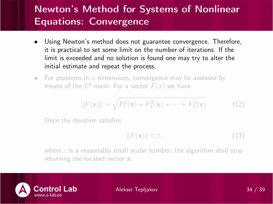
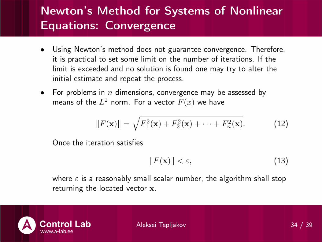
• Using Newton’s method does not guarantee convergence. Therefore,it is practical to set some limit on the number of iterations. If thelimit is exceeded and no solution is found one may try to alter theinitial estimate and repeat the process.
• For problems in n dimensions, convergence may be assessed bymeans of the L2 norm. For a vector F (x) we have
‖F (x)‖ =√
F 21 (x) + F 2
2 (x) + · · ·+ F 2n(x). (12)
Once the iteration satisfies
‖F (x)‖ < ε, (13)
where ε is a reasonably small scalar number, the algorithm shall stopreturning the located vector x.
Newton’s Method for Systems of NonlinearEquations: Convergence
Aleksei Tepljakov 34 / 39
• Using Newton’s method does not guarantee convergence. Therefore,it is practical to set some limit on the number of iterations. If thelimit is exceeded and no solution is found one may try to alter theinitial estimate and repeat the process.
• For problems in n dimensions, convergence may be assessed bymeans of the L2 norm. For a vector F (x) we have
‖F (x)‖ =√
F 21 (x) + F 2
2 (x) + · · ·+ F 2n(x). (12)
Once the iteration satisfies
‖F (x)‖ < ε, (13)
where ε is a reasonably small scalar number, the algorithm shall stopreturning the located vector x.

Newton’s Method for Systems of NonlinearEquations (Example)
Aleksei Tepljakov 35 / 39
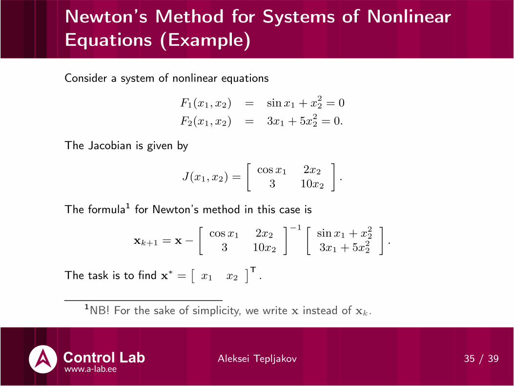
Consider a system of nonlinear equations
F1(x1, x2) = sinx1 + x22 = 0
F2(x1, x2) = 3x1 + 5x22 = 0.
The Jacobian is given by
J(x1, x2) =
[
cosx1 2x2
3 10x2
]
.
The formula1 for Newton’s method in this case is
xk+1 = x−
[
cos x1 2x2
3 10x2
]
−1 [
sinx1 + x22
3x1 + 5x22
]
.
The task is to find x∗ =
[
x1 x2
]T
.
1NB! For the sake of simplicity, we write x instead of xk.

Newton’s Method for Systems of NonlinearEquations (Example)
Aleksei Tepljakov 35 / 39
Consider a system of nonlinear equations
F1(x1, x2) = sinx1 + x22 = 0
F2(x1, x2) = 3x1 + 5x22 = 0.
The Jacobian is given by
J(x1, x2) =
[
cosx1 2x2
3 10x2
]
.
The formula1 for Newton’s method in this case is
xk+1 = x−
[
cos x1 2x2
3 10x2
]
−1 [
sinx1 + x22
3x1 + 5x22
]
.
The task is to find x∗ =
[
x1 x2
]T
.
1NB! For the sake of simplicity, we write x instead of xk.

Some Issues of Newton’s Method
Aleksei Tepljakov 36 / 39
The following list outlines some of the issues encountered withNewton’s method.
• Poor initial estimate. This directly affects the convergence ofthe algorithm. If there is a large error in the initial estimate, themethod may fail to converge, or converge slowly.
• Encountering a stationary point. If the method encounters astationary point of f , where the derivative is zero, the methodwill terminate due to division by zero.
• Overshoot. If the derivative of f is not well behaved in thevicinity of a root, the method may overshoot, and diverge fromthe root.
Modifications of Newton’s method exist that tackle these problems.

Linear Least Squares: Basics
Aleksei Tepljakov 37 / 39
Least squares methods solve problems of type
minx
r21 + · · ·+ r2n =n∑
i=1
(yi − fi(x, ti))2, (14)
where (ti, yi) is the observed data points, fi is the modeling function,and ri are called residuals.
A particularly useful application of least squares fitting exists for systemsof equations
Ax = b. (15)
If there exists no solution for this system, we can instead solve
ATAx̂ = ATb (16)
to obtain an approximate solution that minimizes E = ‖Ax− b‖2.

Linear Least Squares: Example
Aleksei Tepljakov 38 / 39
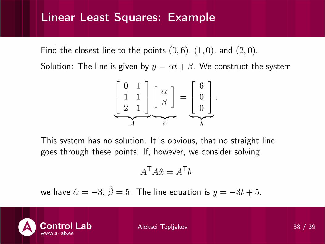
Find the closest line to the points (0, 6), (1, 0), and (2, 0).
Solution: The line is given by y = αt+ β. We construct the system
0 11 12 1
︸ ︷︷ ︸
A
[αβ
]
︸ ︷︷ ︸
x
=
600
︸ ︷︷ ︸
b
.
This system has no solution. It is obvious, that no straight linegoes through these points. If, however, we consider solving
ATAx̂ = ATb
we have α̂ = −3, β̂ = 5. The line equation is y = −3t+ 5.

Linear Least Squares: Example
Aleksei Tepljakov 38 / 39
Find the closest line to the points (0, 6), (1, 0), and (2, 0).
Solution: The line is given by y = αt+ β. We construct the system
0 11 12 1
︸ ︷︷ ︸
A
[αβ
]
︸ ︷︷ ︸
x
=
600
︸ ︷︷ ︸
b
.
This system has no solution. It is obvious, that no straight linegoes through these points.
If, however, we consider solving
ATAx̂ = ATb
we have α̂ = −3, β̂ = 5. The line equation is y = −3t+ 5.
Linear Least Squares: Example
Aleksei Tepljakov 38 / 39
Find the closest line to the points (0, 6), (1, 0), and (2, 0).
Solution: The line is given by y = αt+ β. We construct the system
0 11 12 1
︸ ︷︷ ︸
A
[αβ
]
︸ ︷︷ ︸
x
=
600
︸ ︷︷ ︸
b
.
This system has no solution. It is obvious, that no straight linegoes through these points. If, however, we consider solving
ATAx̂ = ATb
we have α̂ = −3, β̂ = 5. The line equation is y = −3t+ 5.

Questions?
Aleksei Tepljakov 39 / 39
Thank you for your attention!