iaea regional training course use of nuclear techniques
TRANSCRIPT

AAEC/S24
AUSTRALIAN ATOMIC ENERGY COMMISSIONRESEARCH ESTABLISHMENTLUCAS HEIGHTS RESEARCH LABORATORIES
IAEA Regional Training Course
OCTOBER 1982ISBN 0 642 59742 1
Use of Nuclear Techniquesin the Mineral Industry
EDITE BY
J.S. WattB.D.Sowerby

ACKNOWLEDGEMENT OF COPYRIGHT
A number of diagrams, tables and photographs in this volume have
been extracted or adapted from other published works. This is done in
accordance with Section 41 of the Copyright Act 1968 as applied to fair
dealing of copyright material in review and research papers. The sources
of all such material are given in the reference list and captions.
Permission to reproduce such material has been sought from the following
publishers and principals:
McGraw-Hill Inc., Mew York and Wallingford; Pergamon Press, Oxford
and New York? The OS Public Health Service; The Analyst (Royal
Society of Chemistry, London); Minerals Science fi Engineering
(Council for Mineral Technology, formerly National Institute of
Metallurgy, South Africa); John Wiley G Sons Inc., New York and
London; Academic Press, New York; Professor W. Hornyak, University
of Maryland.
The authors thank the following organisations for the use of
unpublished or non-copyright material provided by private communication
or in trade literature:
US Bureau of Mines; The Radiochemical Centre, Harwell, UK; Society
of Mining Engineers (AIME); Harshaw Chemical Co; Outokumpu Oy,
Finland; Commonwealth Scientific & Industrial Research Organization;
Australian Mineral Development Laboratories.
Some material has been selected from IAEA Conference Proceedings
for which copyright clearance had been obtained by individual authors.
Production Editor:
Layout:
Word Processing:
Graphics Design:
Peter J.F. Newton
Shirley Gamblin
Christine Avis; Helen Sarbutt
Jeff Brown
AUSTRALIAN ATOMIC COMMONWEALTH SCIENTIFIC
FNFRPY rOMMT^TON **"> INDUSTRIALENERGY COMMISSION RESEARCH ORGANIZATION
IAEA REGIONAL TRAINING COURSE
USE OF NUCLEAR TECHNIQUES IN THE MINERALS INDUSTRY
EDITED BY
J.S. WATT
B.D. SOWERBY
PRINTED AT THE AAEC RESEARCH ESTABLISHMENT
LUCAS HEIGHTS RESEARCH LABORATORIES

National Library of Australia card number and ISBN 0 642 59742 1
The following descriptors have been selected from the INIS Thesaurus todescribe the subject content of this report for information retrievalpurposes. For further details please refer to IAEA-INIS-12 (INIS: Manual for
Indexing) and IAEA-INIS-13 (INIS: Thesaurus) published in Vienna by theInternational Atomic Energy Agency.
CHAPTER 1 ALPHA PARTICLES; BETA PARTICLES; BINDING ENERGY; ELECTRONICSTRUCTURE; FISSION; GAMMA RADIATION; ISOTOPE PRODUCTION; NUCLEARDECAY; NUCLEAR PHYSICS; NUCLEAR PROPERTIES; NUCLEAR REACTIONKINETICS; THERMONUCLEAR REACTIONS
CHAPTER 2 • ELECTRONIC EQUIPMENT; RADIATION DETECTION; RADIATION DETECTORS;SPECTROSCOPY; STATISTICS
CHAPTER 3 GAMMA SOURCES; NEUTRON SOURCES; X-RAY SOURCES
CHAPTER 4 RADIOMETRIC GAGES; DENSIMETERS; LEVEL INDICATORS; MOISTURE GAGES;THICKNESS GAGES •
CHAPTER 5 ON-LINE MEASUREMENT SYSTEMS; ORES; RADIATION ABSORPTION ANALYSIS;RADIATION DETECTORS; SLURRIES; X RADIATION; X-RAY FLUORESCENCEANALYSIS; X-RAY FLUORESCENCE LOGGING
CHAPTER 6 COAL; GAMMA RADIATION; NEUTRON ACTIVATION ANALYSIS; IRON ORES;NUCLEAR REACTION ANALYSIS; RADIATION ABSORPTION ANALYSIS;RADIATION SCATTERING ANALYSIS; RADIOACTIVITY LOGGING; SAMPLING; XRADIATION
CHAPTER 7 BOREHOLES; CALIBRATION; ERRORS; GAMMA-GAMMA LOGGING; NEUTRONLOGGING; RADIATION DETECTORS; WELL LOGGING EQUIPMENT
CHAPTERS FLOW RATE; GROUND WATER; HYDROLOGY; RADIOSOTOPES; SEDIMENTATION;TRACER TECHNIQUES; WASTE MANAGEMENT; WEAR
CHAPTER 9 DOSE LIMITS; PERSONNEL DOSIMETRY; RADIATION DOSES; RADIATIONHAZARDS; RADIATION PROTECTION; RADIOACTIVE MATERIALS; TRANSPORT

(iii)
CONTENTS
INTRODUCTION
J.S. Watt
Page
(vi)
AUTHOR - LECTURERS (vii)
CHAPTER 1. BASIC NUCLEAR PHYSICS
J.R. Harries
CHAPTER 2.
A.
B.
C.
D.
E.
THE DETECTION AND MEASUREMENT OF
NUCLEAR RADIATION
RADIATION DETECTION AND MEASUREMENT
E.M. Lawson
EXAMPLES OF RADIATION DETECTION
E.M. Lawson
ELECTRONICS
E.M. Lawson
STATISTICS FOR NUCLEAR MEASUREMENT
E.M. Lawson
NUCLEAR SPECTROMETRY AND SPECTRAL
INTERPRETATION
P.L Eisler
51
53
61
75
85
97
CHAPTER 3. GAMMA RAY AND NEUTRON SOURCES
R.J. Holmes
123
CHAPTER 4.
CHAPTER 5.
A.
B.
NUCLEONIC GAUGES
B.D. Sowerby
137
X-RAY ANALYSIS 149
INTRODUCTION TO X-RAY FLUORESCENCE(XRF) 151
AND X-RAY PREFERENTIAL ABSORPTION(XRA)
ANALYSIS
L.S. Dale, J.S, Watt
TECHNIQUES FOR GENERAL PURPOSE XRF 165
AND XRA ANALYSIS
R*A. Fookes, J.S. Watt

(iv)
C. X-RAY TECHNIQUES FOR ON-STREAM
ANALYSIS OF MINERAL SLURRIES
R.A. Fookes, J.S. Watt
D. ON-STREAM ANALYSIS SYSTEMS
W.J. Howarth, J.S. Watt
E. APPLICATIONS OF ON-STREAM ANALYSIS
SYSTEMS
W.J. Howarth
F. BENCH TOP AND PORTABLE MINERAL
ANALYSERS, BOREHOLE CORE ANALYSERS
AND IN SITU BOREHOLE LOGGING
W.J. Howarth, J.S. Watt
Page
175
185
199
211
CHAPTER 6.
A.
B.
C.
D.
E.
BULK ANALYSIS AND SAMPLING 227
GAMMA- RAY METHODS 229
B . D . Sowerby
NEUTRON ACTIVATION FOR BULK ANALYSIS 241
M. Borsaru
PROMPT NEUTRON-GAMMA METHODS 255
B . D . Sowerby
BULK ANALYSIS OF COAL 269
B . D . Sowerby
SAMPLING PRACTICES IN THE MINERAL 287
INDUSTRIES
R.J. Holmes
CHAPTER 7.
A.
B.
C.
FIELD MEASUREMENTS IN BOREHOLES 309
NATURAL GAMMA SPECTROSCOPY FOR 311
BOREHOLE LOGGING
J. Aylmer
THEORY AND PRACTICE OF GAMMA-GAMMA 337
METHODS IN NUCLEAR GEOPHYSICS
P.J. Mathew
EXPLORATION AND GRADE CONTROL 359
NEUTRON LOGGING
P.L. Eisler

(v)
CHAPTER 8.
A.
B.
CHAPTER 9.
A.
B.
ENGINEERING ASPECTS OF RADIOMETRIC
LOGGING
P. HUppert
APPLICATIONS OF RADIOISOTOPE TRACERS
NUCLEAR HYDROLOGY AND SEDIMENTOLOGY
P.L. Airey
MINERAL PROCESSING
J.F. Easey
EFFLUENT MANAGEMENT
J.F. Easey
RADIATION SAFETY
IONISING RADIATIONS
D.A. Woods
SOME HEALTH PHYSICS CONSIDERATIONS
D.A. Woods
Page
383
401
403
417
431
439
441
453

(vi)
INTRODUCTION
These lecture notes describe principles and applications of nuclear
techniques in the mineral industry. The notes cover basic nuclear
physics, detection and measurement of radiation, radiation safety,
application of X-ray analysis techniquts particularly to on-stream
analysis of mineral slurries, sampling 'and bulk analysis applications,
in situ borehole analysis, and applications of radio-tracers. The
lectures were part of a regional training course for university graduates
in the physical sciences or engineering who were currently working in
the mineral industry. The course was designed to provide sufficient
training to enable participants to evaluate and use commercially avail-
able nucleonic instrumentation.
The Regional Training Course for Asia and the Pacific on Use
of Nuclear Techniques in the Mineral Industry was held in Australia from
23 June to 25 July 1980. The International Atomic Energy Agency invited
the Government of Austra.lia to undertake this course. It was organised
by the Australian Atomic Energy Commission (AAEC) and the Commonwealth
Scientific and Industrial Research Organization (CSIRO), and was financially
supported by the Australian Government.
The Regional Training Course consisted of the following components:
(a) Two and a half weeks of lectures and experiments at the
Australian School of Nuclear Technology, Lucas Heights on the
use of nuclear techniques in the mineral industry.
(b) A three-day course on control of mineral concentrators at the
Julius Kruttschnitt Mineral Research Centre, University of
Queensland, Bri sbane.
(c) Two weeks of visits, mainly to mining centres and to mineral
companies, to view nucleonic systems in routine use in industry.
J.S. WATT
Course Director
CSIRO Division of Mineral Physics
June 1982
(vii)
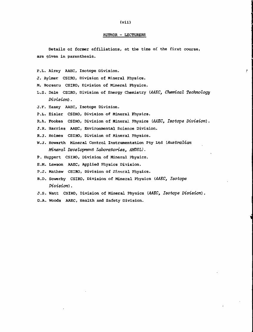
AUTHOR - LECTURERS
Details of former affiliations, at the time of the first course,
are given in parenthesis.
P.L. Airey AAEC, Isotope Division.
J. Aylmer CSIRO, Division of Mineral Physics.
M. Borsaru CSIRO, Division of Mineral Physics.
L.S. Dale CSIRO, Division of Energy Chemistry (AAEC, Chemical Technology
Division) .
J.F. Easey AAEC, Isotope Division.
P.L. Eisler CSIRO, Division of Mineral Physics.
R.A. Fookes CSIRO, Division of Mineral Physics (AAEC3 Isotope Division).
J.R. Harries AAEC, Environmental Science Division.
R.J. Holmes CSIRO, Division of Mineral Physics.
W.J. Howarth Mineral Control Instrumentation Pty Ltd (Australian
Mineral Development Laboratories* AMDEL).
P. Huppert CSIRO, Division of Mineral Physics.
E.M. Lawson AAEC, Applied Physics Division.
P.J. Mathew CSIRO, Division of i-linoral Physics.
B.D. Sowerby CSIRO, Division of Mineral Physics (AAEC, Isotope
Division).
J.S. Watt CSIRO, Division of Mineral Physics (AAEC3 Isotope Division).
D.A. Woods AAEC, Health and Safety Division.

CHAPTER 1
BASIC NUCLEAR PHYSICS
J.R. Harries

1. ATOMS
Although these notes deal mainly with nuclear properties, it is
desirable to discuss first the structure of the atom as a whole. The
atomic electrons are important in some radioactive decays and they are
responsible for X-ray emission.
1.1 Atomic Structure
An atom consists of a small, dense nucleus containing over 99.97
per cent of the atomic mass, and a surrounding cloud of electrons. The
nuclear radius is only about 6 x 10 15 m compared to the atomic radius
of about 10~10 m (i.e.. atomic radius « 17 000 x nuclear radius).
The nucleus consists of protons (positive charge) and neutrons
(neutral) bound together by nuclear forces. The electrons (negative
charge) are bound to the nucleus by electrostatic attraction. The
electron and proton charges are precisely equal, although of opposite
sign, and neutral atoms contain equal numbers of protons and electrons.
Electrons move in different orbits or, more correctly, states
around the nucleus. The electrons in an atom can only occupy certain
discrete states with particular energies and angular momenta. Electrons
can transfer from one state to another, provided that a vacancy exists
and energy is conserved.
The electron states of an atom can be specified by a set of four
quantum numbers:
(a) The principal' quantum number, n, which takes values n = 1,
2, 3, 4, The principal quantum number labels the discrete
energy states that the electron can occupy. The most-bound
state, nearest to the nucleus, is known as the K shell and has
n = 1. Successive less-bound shells are known as the L shell
(n = 2), M shell (n = 3) and so on up to the Q shell (n = 7).
(b) The angular momentum quantum number £, which takes values
A = 0, 1, 2, , (n-1). The number of permissible values
of angular momenta is equal to the principal quantum number.
For example, in the M shell (n = 3) £ can have values of 0, 1
or 2. These subshells are often labelled by the letters
s, p, d, f, for values of A = 0, 1, 2, 3, respectively.
(c) The magnetic quantum number3 m, which takes values m = -H,
-S, + 1, ..., 0,...,& - 1, !L. For example, in the d subshell
(A = 2) m can have the values -2, -1, 0, 1, 2. Note that
there are (2£, + 1) different values of m for each value of A.
The m quantum number labels the allowed orientation of the
quantised angular momentum.
(d) The spin quantum number, s, which can only be +% or -h. The
electron has a small intrinsic spin and in any interaction
these are the only two allowed orientations.
A fundamental property of the electron is expressed by the-PouZi
exclusion principle, namely that no two electrons can occupy the same
state. Hence in an atom, no two electrons occupy states with the same
set of quantum numbers n, £., m, s.
When a free electron is captured by a nucleus, the excess energy is
released. This energy is called the binding energy. To remove the
electron from the atom requires that energy, equal to the binding energy,
must be supplied to the electron. The binding energy decreases with
increasing values of principal quantum number, n, and, to a lesser
extent, with increasing values of the angular momentum quantum number.
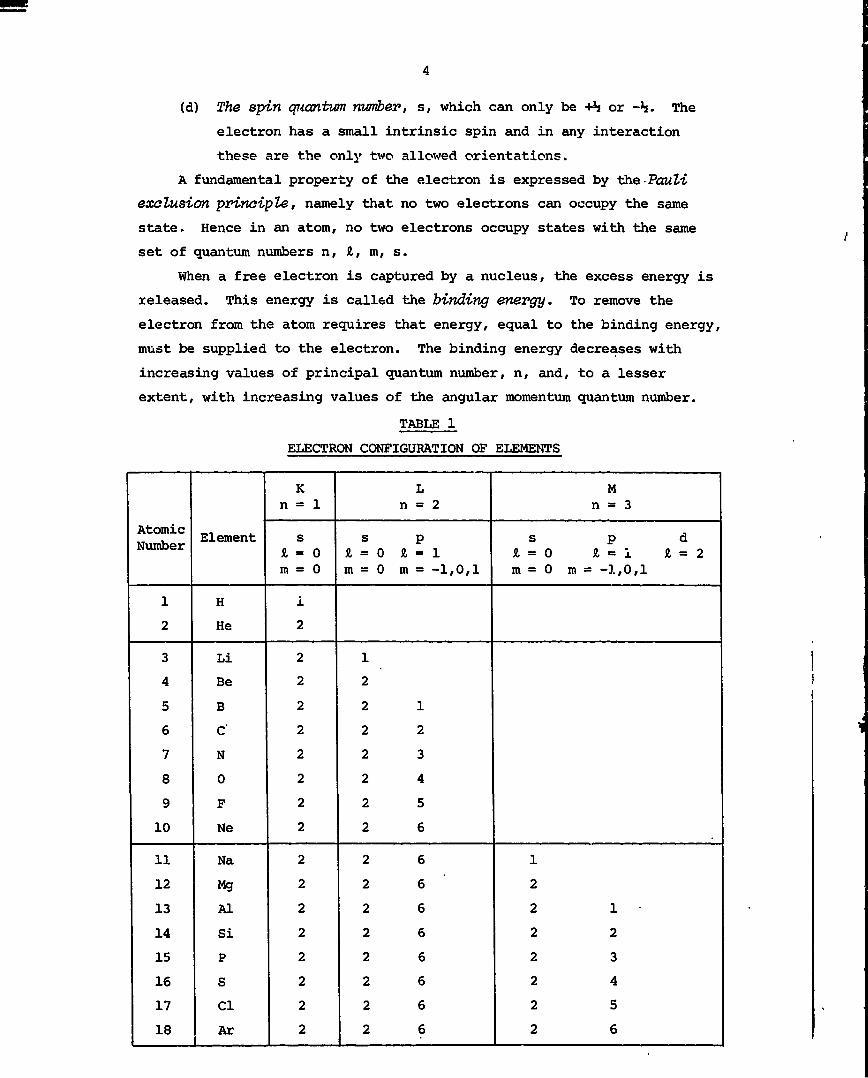
TABLE 1
ELECTRON CONFIGURATION OF ELEMENTS
AtomicNumber
1
2
3
4
5
6
7
8
9
10
11
12
13
14
15
16
17
18
Element
H
He
Li
Be
B
C'
N
0
F
Ne
Na
Mg
Al
Si
P
S
Cl
Ar
Kn = 1
sS, = 0m = 0
1
2
2
2
2
2
2
2
2
2
2
2
2
2
2
2
2
2
Ln = 2
s p£ = 0 £ = 1m = 0 m = -1,0,1
1
2
2 1
2 2
2 3
2 4
2 5
2 6
2 6
2 6
2 6
2 6
2 6
2 6
2 6
2 6
Mn - 3
s p di = 0 £ = 1 A = 2m = 0 m = -1,0,1
1
2
2 1
2 2
2 3
2 4
2 5
2 6

The build-up of the'electron configuration of elements with successive
atomic numbers is shown in table 1. The hydrogen atom has only one
electron which is in the lowest energy state (i.e. highest binding
energy) n = 1, Jl = 0, m = 0, s = +!zor-J5. Helium has two electrons;
one is the n — 1, & = 0, m=0, s = +1j state and one is the n = 1,
I = 0, m=0, s = -** state. In lithium, the third electron is in the L
shell, n = 2, 9. - 0, m = 0, s = +h, or -*$. Boron, with five electrons,
has one electron in the p subshell, n=2, £, = 1, m = 0, s = h. Eight
electrons fill the L shell, that is two electrons in the s subshell
(A = 0) and six electrons in the p subshell (£. = 1) .
Each successive element has one extra proton as well as one extra
electron, so the attraction to the nucleus for all the inner electrons
increases as each new element is formed. The binding energy of the K
shell electron in hydrogen is a thousand times less than the binding
energy of the K shell electron in krypton. The binding energy of the
outermost electron is similar for all atoms, and it is the same as the
ionisation potential. Chemical reactions depend on the interaction
between the outer electrons of different elements.500
200 -
100
so K
10 -
10 20 30 40 50 60 TO 80 90 100
ATOMIC NUMBER (Z)
FIGURE 1
THE ENERGY OF X-RAYS EMITTED FROM THE DIFFERENTATOMIC SHELLS AS A FUNCTION OF ATOMIC NUMBER

1.2 X-ray Emission
If an electron is removed from one of the inner shells, an electron
from further out will drop into the vacancy. The outer electron is more
tightly bound in the new position (it falls further into a well) and the
excess energy is radiated away as X-rays or ultraviolet radiation. A
vacancy in the innermost K shell might be filled from the L shell, M
shell or higher. K shell vacancies produce K X-rays with slightly
differing energies, depending on the origin of the electron that fills
the vacancy. A K X-ray will usually be followed by L and/or M X-rays as
subsequent vacancies are filled.
Figure 1 shows the energies of the X-rays emitted from the K, L,
and M shells. Some modes of radioactive decay produce vacancies in the
atomic electron shells, and hence X-rays are emitted.
Sometimes, instead of X-rays being emitted, the energy is used to
eject an electron from one of the outer shells. Electrons emitted
instead of X-rays are known as Auger electrons and they have a discrete
energy. The number of X-rays emitted per vacancy in a given shell is
known as the fluorescent yield. The fluorescent yield for the K shell
increases with atomic number, from 0.1 for potassium to 0.96 for lead.
1.3 Electron Volt and Avogadro's Number
Electron volt
An electron volt (eV) is the energy gained by an electron in passing
through a potential of 1 volt:
1 eV = 1.60207 x 10~19 J
The electron volt is widely used as the unit of energy in atomic
and nuclear processes, e.g. 1.33 MeV y-ray from cobalt-60, 5.9 keV
X-ray from manganese-55.
An electron with an energy of 1 eV has a velocity of 600 km s *,
and a proton of 1 eV has a velocity of 14 km s *.
Avogadro's number
Avogadro's number = number of atoms in 12 grams of carbon-12
= 6.022 x 10²³
The SI system of units defines the mole as the amount of substance of a
system .that contains as many elementary entities as there are atoms in
12 grams of carbon-12.

For a sample of molecules or atoms, a mole is the amount of material
whose mass, expressed in grams, is numerically equal to the molecular or
atomic weight:
e.g. Copper, atomic weight 63.546
1 mole copper = 63.546 g
and this will contain 6.022 x 10²³ atoms
1 g copper contains 6.022 x 10²³/63.546
= 9.5 x 10²¹ atoms
2. NUCLEAR PROPERTIES
2.1 Nuclear Size
The size of the nucleus can be determined by scattering a-particles
on the nuclei. The nucleus is composed of a number of subunits, tightly
packed so that the nuclear matter is incompressible and has a constant
density of about 10 17 kg m 3. From the scattering and other experiments,
the nuclear radius R has been derived as:
where A is the atomic mass number
and R = (1.3 ± 0.1) x 10 mo ~15
= 1.3 ± 0.1 fm
2.2 Nuclear Constituents
The nucleus consists of protons and neutrons held together by
internucleon forces. Protons and neutrons are collectively called
nucleons. Table 2 shows how different nuclei can be built up from nucleons.
The atomic number Z is the number of protons
The neutron number N is the number of neutrons
The atomic mass number A is the total number of nucleons
A = N + Z
It is customary to designate a nucleus in the following way:
AY °* AYZA Z AN
The number of electrons in the shells of the atom is exactly equal
to the number of protons (Z) in the nucleus.

TABLE 2
BUILD UP OF NUCLEI FROM NUCLEONS
Element
Hydrogen
Helium
Lithium
Iron
Lead
L
Z
1
1
2
2
3
3
26
26
26
26
82
82
82
82
N
0
1
1
2
3
4
28
30
31
32
122
124
125
126
A
1
2
3
4
6
7
54
56
57
58
204
206
207
208
Symbol
XH2H3He4He6Li7Li54*Fe56Fe57S/Fe58Fe204^u*Pb206u°Pb207Pb
2°8Pb
Abundancein Nature
(%)
99.985
0.015
0.00013
99.99987
7.5
92.5
5.8
91.8
2.1
0.3
1.42
24.1
22.1
52.4
A nuclide is a —artain species of nucleon characterised by its
Z and N. Isotopes are nuclides with the same Z but different N.
They have the same chemical properties:
e.g. 6329Cu
6529Cu
Isotanes are nuclides with the same N but different Z:
e.g. 2612Mg
2713Al
2814Si
Isobars are nuclides with the same A:
e.g. 3114siS1
3115
3116
Isomers are nuclides with the same A and Z but with extra
excitation energy above the ground state:
e.g. (t = 6 h) , (t = 200 000 y)

2.3 Nuclear Forces
The attractive nuclear force between nucleons holds the nucleus
together in spite of the repulsive electrostatic, or coulomb, forces
between the positively charged protons. The internucleon force is very
strong but only acts over short ranges of about 10 15 m. At larger
distances, the internucleon force is negligible and the electrostatic
force is most important.
A positively charged particle approaching the nucleus will be
repelled. This repulsive force is referred to as the coulomb barrier.
For an o-particle and a uranium-238 nucleus, the coulomb barrier is
24.2 MeV. An ex-particle requires at least 24.2 MeV to make contact with
tha uranium nucleus. Once inside the nucleus, the attractive internucleon
forces overwhelm the coulomb repulsion and the nucleons are tightly
bound.
2.4 Nuclear Masses
The results of measurements of isotopic masses with mass spectrographs
show that the atomic masses of all the nuclides are very nearly integers
on a scale in which the atomic mass of the most abundant isotope of
carbon is assigned the exact value of 12. The unit of atomic mass, that
is one a.m.u., is thus defined:
Mass of 12C = 12.0000 a.m.u.
1 a.m.u. = 1.6604 x 10~27 kg
The atomic mass (M) is the mass of the atom (including the electrons)
measured in atomic mass units. The atomic mass number A is the nearest
integer to this:
e.g. 31P A = 31 M = 30.973763 a.m.u.
Neutron A - 1 M = 1.00866 a.m.u.
Hydrogen A = 1 M = 1.00782 a.m.u.
From Einstein's theory of relativity comes the important relationship
of the equivalence of mass and energy:
E = me2
where c is the velocity of light = 3 x 10® m s *
hence 1 kg = 5.61 x 1029 MeV = 8.99 x 10¹⁶ J
and 1 a.m.u. = 931.48 MeV
Thus mass can be changed into energy or vice versa, provided that the
change is according to the above relationship.

10
2.5 Nuclear Binding Energy
For a nucleus containing Z protons and N neutrons, the nuclear
mass, M , is less than the sum of the masses of the nucleons:
KI < Zm + NmN p n
or equivalently, since it is the mass of the neutral atom that is measured,
K < Zm + Nm + Zma p n e
or M < Zm__ + Nma H n
where nu is the mass of the hydrogen atom. When the protons and neutrons
are combined, they give up energy which shows as a mass reduction. If
the nucleus is to be split up into its original constituents, then
energy must be supplied. This energy is called the binding energy of
the nucleus:
M 4- B.E = Zm, + Nma H n
Binding energy is a measure of the stability of the nucleus. The greater
the energy needed to unbind the system, the more stable it is.
Conside
two protons:
4Consider the hypothetical formation of He from two neutrons and
1 1 42 XH + 2 Qn •*• 2He
The mass defect is
A M = 2 M + 2 M H - M t f e » (2 x 1.00866) + (2 x 1.00782) - (4.00260)
- 0.03036 a.m.u.
= 28.3 MeV4
This means that to break a He nucleus into its basic components
would require the addition of 28.3 MeV.
The binding energy per nueleon is a more useful quantity and is
defined as
ZIIL, + Nm - M
'- A" a
for 4He B = 7.1 MeV.
The binding energy per nucleon as a function of mass number is plotted
in figure 2. The average binding energy/nucleon (an average over the
whole mass range) is 7.6 MeV.

11
" 0 4 8 12162024 j() (JQ 90 120 150 180 210 240
MASS NUMBER A
FIGURE 2
BINDING ENERGY PER NUCLEON V. MASS NUMBER FORNATURALLY OCCURRING NUCLIDES (AND 8Be). Notethe scale change on the abscissa at A = 30.
The important features of the graph in figure 2 are:
(i) A rapid increase of B with mass number for the light nuclei
with stability peaks for He, C, 0 and minima for Li
(ii)
* 10Dand B.
A slow variation with mass number from mass ** 30. The
variation is slow because each nucleon experiences an attractive
force which is caused by a small number of close neighbours and
not by all the nucleons in a nucleus (otherwise B would increase
with mass number).
(iii) B increases up to mass » 60. This is a surface tension effect.
Nucleons near the surface have fewer neighbours and so experience
less attractive force than those deep inside. This effect
decreases as.radius (and mass number) increases.
(iv) B decreases for masses greater than 60. A proton experiences
a nuclear force from a small number of close neighbours, but
it also experiences an electrostatic repulsion by all protons
within the nucleus. The repulsion becomes more important for
large nuclei and causes a reduction in B. For nuclei above
mass number 209, the electrostatic repulsion is so great that
there are no further stable nuclei.

12
2.6 Nuclear Fission and Fusion
Figure 2 shows that the binding energy per nucleon has decreased
significantly by mass numbers A ~ 220. It helps to think of such nuclei
in terms of a liquid drop. The shape of the drop depends on a balance
involving surface tension and coulomb forces. If a neutron is captured,
the excitation energy causes the drop to oscillate. The shape distorts
and, if the excitation is sufficient, the drop becomes shaped like a
dumb-bell and coulomb repulsion between the two ends can produce two
drops of comparable size. This process is known as fission. The binding
energy/nucleon of the fragments is greater than the binding energy/nucleon
of the original nucleus. Two or three neutrons and also kinetic energy
are released. The two fragments have atomic masses between 80 and 150,
with most probable values of 95 and 140.
Consider the following example:
235Mass of U -I- n = 235.0439 + 1.0087 = 236.0526 a.m.u.
Mass of fission fragments = 93.9154 + 138.9179 + 3.0260
= 235.8593 a.m.u.
•'• Mass converted to energy = 0.193 a.m.u.
= 180 MeV
These fission fragments are unstable and decay by beta emission to94 1394f)Zr and c7
La- Tne energy released by the successive beta decays is
about 19 MeV.
Hence total energy release = 199 MeV
energy release/nucleon = 0.85 MeV
The above calculation for the energy released in fission was based
on the mass 'defect' (mass loss). The calculation can also be performed
by considering binding energies per nucleon (see figure. 2) . The binding235
energy/ nucleon for U is 7.6 MeV and in the region of mass 117 (fissi
products) it is 8.5 MeV.275
Initially the binding energy of U is 235 x 7.6 - 1786 MeV and94 139after fission, the binding energy of Zr and La = 233 x 8.5 = 1980.
Hence the energy released = 1980 - 1786 = 194 MeV.

13
These energy considerations suggest that all heavy nuclides should
fission spontaneously. This does not happen because the nucleus has to
be deformed to fission and the deformation requires energy. The probability
of spontaneous fission and neutron-induced fission varies with different
nuclides.
The neutrons released in a fission reaction nay cause more fission
events, which in turn lead to more neutrons. This is known as a chain
reaction.
The low binding energy of nuclides with small mass numbers means
that large amounts of energy can be released if the nuclides combine to
form heavier nuclides. This process is known as fusion. Sufficient
energy to overcome the electrostatic repulsion between the nuclei must
be supplied before the reaction can occur. This can be achieved byo
raising the temperature to ~ 10 degrees, e.g. in a plasma.
The deuterium -tritium (D-T) reaction will be used in the first
generation fusion reactors, i.e.
He
Mass of
Mass of
[H + ][H = 2.01410 + 3.01605
= 5.03015 a.m.u.
Sle + n - 4.00260 + 1.00867
= 5.01127 a.m.u.
Mass converted to energy = 0.01888 a.m.u.
= 17.6 MeV
This energy appears as kinetic energy of the o-particle (3.5 MeV) and
the neutron (14.1 MeV).
At higher plasma temperatures, the following fusion reactions can
be used:
H H :He + n 3.27 MeV
H E = 4.04 MeV
H He ,He E = 18.34 MeV

14
2.7 Nuclear Stability
The number of possible combinations of protons and neutrons is very
large. However the number of naturally-occurring stable nuclei is
relatively small ("270). These cluster about a line of nuclear stability
which, for light masses, has N * 1.5 Z. The number of observed unstable
nuclei with measurable half-lives is over 1000. A neutron-rich nucleus
is most likely to decay by 3 emission. A proton-rich nucleus is most
likely to decay by positron emission or electron capture.
Within the nucleus, a proton can change into a neutron or a neutron
can change into a proton if this will produce a nucleus with a smaller
mass. The time required for this to occur can be quite long, for example
4019K21
4°Ca20Ca20 1.3 x 10s y
The nuclides in a given isobar will decay to the smallest atomic
mass. Figure 3 shows atomic mass parabolas for mass number A = 135 and
A = 102. For odd A nuclei, there is only one stable nuclide for each
value of A. The binding energy for even A nuclides is greater if there
is an even number of protons arid an even number of neutrons, i.e. even Z
and even N, than if there is an odd number of protons and an odd number
of neutrons. This results in the two atomic mass parabolas shown in
figure 3b. Even A isobars often have two or even three stable nuclides
at the bottom of the curve.
FIGURE 3
MASS PARABOLA FOR ISOBARS. (a) Odd A nuclei,(b) Even A nuclei. Full circles representstable nuclides and open circles radioactivenuclides. Along the ordinate, one divisionis approximately equal to 1 MeV.

15
2.8 Nuclear Energy Levels and Decay Schemes
If a nucleus is formed in an excited state, it can return to its
ground state by losing energy in the form of electromagnetic radiation;
this is called y radiation. There is no change in N, Z or A. It is
found, when studying the y decay of an excited nucleus, that the y-rays
have discrete energies, giving rise to the concept of nuclear energy
levels, somewhat analogous to the discrete energy states of the electrons.
A nucleus in an excited state may decay directly to the ground state, or
to another excited state and then to the ground state. In the first
case, the y-radiation is referred to as primary, and decays from an
intermediate state to the ground state are referred to as secondary.12
A decay scheme showing the low-lying levels of C is shown in
figure 4. In light nuclei and at low excitations, energy levels are
well separated by several MeV. For heavier nuclei and higher excitations,
the level density increases very rapidly such that the separation is in
the electron volt range and the levels virtually become a continuum.
Each nucleus has a unique energy level scheme and therefore it is
possible to identify a nucleus from the y-rays that are emitted. Selection
rules and nuclear properties dictate the levels through which the y
transitions may occur. When a particular level has the choice of more
than one possible mode of decay, the ratio of the intensities of the
modes are known as the branching ratio.
3. NUCLEAR DISINTEGRATION AND RADIOACTIVITY
3.1 Alpha-decay
Alpha-particles are helium nuclei, and consist of two protons and
two neutrons. The four nucleons are so tightly bound that an a-particle
is usually emitted in preference to a single nucleon. Alpha decay is
most common for heavy nuclei with Z * 82. In a decay
N
A-4
Z X-2 •«*• N-;
Alpha-particles are emitted with a line spectrum, e.g. when222.
22688
decays to ~~~Rn, the a-particle energies are 4.782 MeV (94.6%), 4.59986
MeV (5.4%) and 4.340 MeV (0.0057%).
For heavy elements, the binding energy per additional nucleon is
about 5.5 MeV which is much less than the average binding energy/nucleon
of 7.6 MeV. Hence the energy required to detach the four -nucleons in
an a-particle from a heavy nucleus is 4 x 5.5 = 22 MeV. Additional

16
O, -?.»• nle
FIGURE 4
ENERGY LEVEL SCHEME OF 12C(After Lederer et al. 1968)
17
energy of about 5 MeV is required to penetrate the coulomb barrier of
the nucleus. The 27 MeV needed to detach the four individual nucleons
is less than the 28 MeV binding energy of the a-particle. Hence for
heavy nuclides (Z £ 82) , a decay is energetically possible.
Once through the coulomb barrier, the a-particle regains the
penetration energy of about 5 MeV as the positively charged a-particle
is repelled from the positively charged nucleus. The half-life for
a-particle emission decreases rapidly as the a energy increases, e.g.
for uranium (Z = 92) 7.5 MeV a-decay has t, ~1 s., 5.7 MeV has t,~l y,
and 4.4 MeV has t, ~109 y. There are very few a decays with a particle
energies less than 3.5 MeV.
3.2 B~ decayA AIf atomic mass ( X ) > atomic mass ( Y ) , then nucleus X
will decay to nucleus Y by g decay. In 3 decay, a neutron in the
nucleus is transformed to a proton with the emission of a negative beta
particle and a neutrino. The g particle is identical to an atomic
electron except that it originates from the nucleus.
o +n -*• p + e v
The neutrino (v) has zero rest mass, no charge and travels at the
speed of light. It is very penetrating and is not usually observed. One
hundred light years of matter is required to give a 50 per cent chance
of absorbing a 1 MeV neutrino.
uZ
• 4
W *HM
§ 2
&
I'<a 0
I I
0.1 0.2 0.3 0.4 0.5
KINETIC ENERGY, E (MeV)
0.7
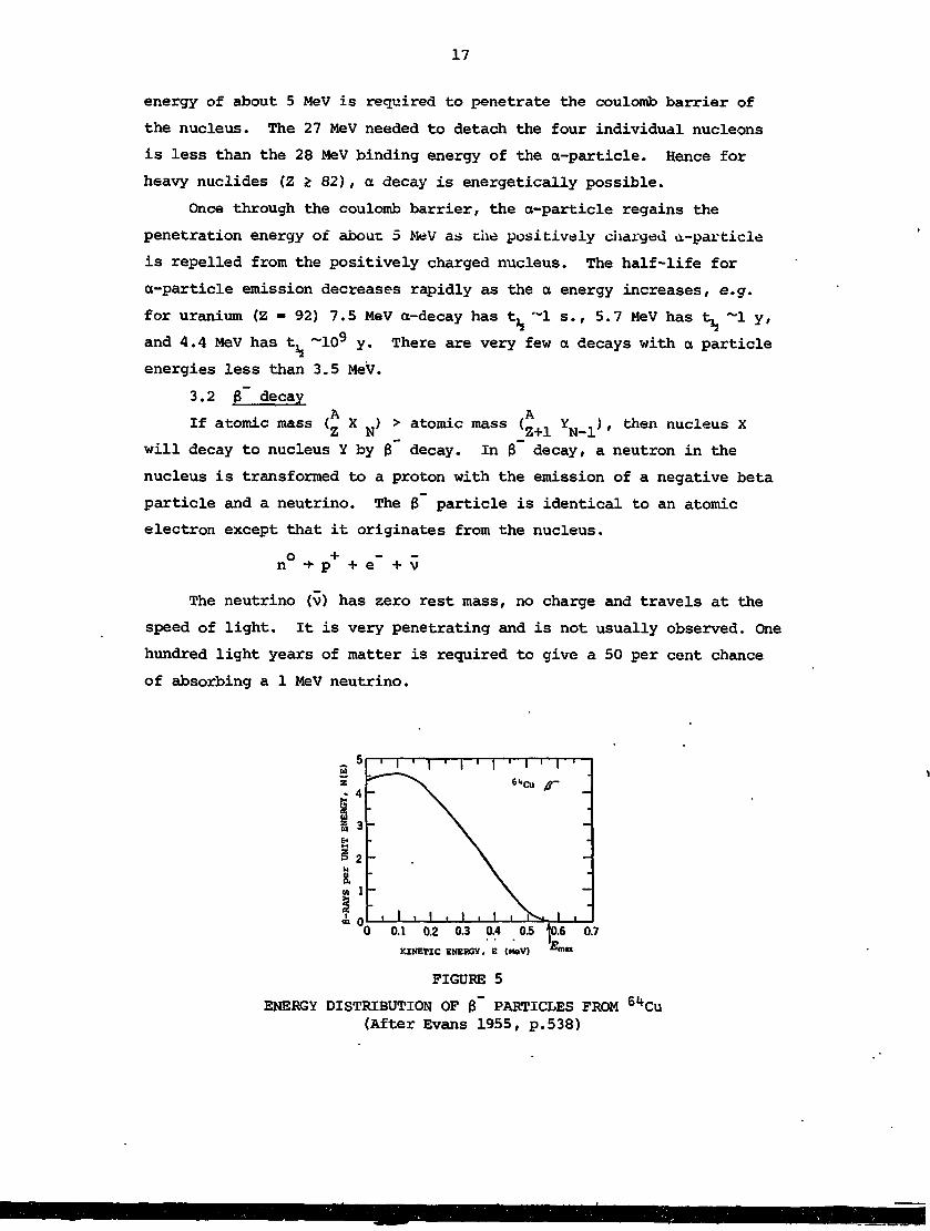
FIGURE 5
ENERGY DISTRIBUTION OF 0~ PARTICLES FROM 6l*Cu(After Evans 1955, p.538)

18
The emitted (3-particles have a broad energy spectrum with a most
probable value about one third of the maximum expected value. A typical
8 decay energy spectrum is shown in figure 5. The maximum 8 energy
corresponds to the energy available from the decay. This energy is
divided between the $ and the neutrino and this produces the broad
energy distribution of fl-particles .
In 8 decay, the number of electrons in the initial and final
states balance. The atomic number of the daughter nucleus is one greater
than the atomic number of the parent nucleus, so the daughter atom
requires one extra atomic electron. However, the 8 decay process
supplies one electron that did not previously exist. Hence although the
atomic electron acquired by the daughter nucleus will be a different
electron to the electron emitted at high velocity in the decay, the net
number of electrons gained from outside by the decayed atom is zero.
Because of this balance 8 decay will occur if the atomic mass of the
daughter atom, i«.e. the energy of the final state, is less than the
atomic mass of the parent atom, i.e. the energy of the intitial state.
Free neutrons, outside the nucleus, are unstable and decay to
protons with the emission of electrons and neutrinos. The half-life of
the free neutron is 10.6 mir? and the energy released in the decay is 780
keV. However, neutrons in the nucleus are stable, unless the required
conditions for 8 decay are met; the half-life then depends on the 8
decay, not on the free neutron half -life.
3.3 8 Decay and Electron CaptureA AIf atomic mass ( X ) > atomic mass (Z_I
YN.I) then X can decay to Y,
with a proton transforming to a neutron.
8 Decay.(. ' _8 decay will occur if .the energy is sufficient. Unlike 8 decay,
8 decay can only occur if the atomic mass X is greater then the atomic
mass Y by at least the rest mass of two electrons, i.e. 0.0011 a.m.u. or
1.022 MeV. In 8 decay the proton changes into a neutron with the
emission of a positron and a neutrino.
+ o +p •»• n + e + v
The positron has a positive charge and the same mass as an electron;
it is an anti-electron. If a positron and an electron meet, they are
annihilated with the emission of two yrays. Each y ay has an energy
19
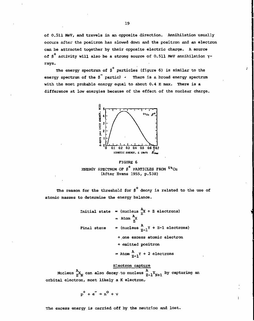
of 0.511 MeV, and travels in an opposite direction. Annihilation usually
occurs after the positron has slowed down and the positron and an electron
can be attracted together by their opposite electric charge. A source
of 3 activity will also be a strong source of 0.511 MeV annihilation y~
rays.
The energy spectrum of 3 particles (figure 6) is similar to the
energy spectrum of the 3 particJ -= There is a broad energy spectrum
with the most probable energy equal to about 0.4 E max. There is a
difference at low energies because of the effect of the nuclear charge.
5 5
I4H 3
i*
1'i 0
0 0.1 0.2 0.3 0.4 0.5 0.6 f 0.7KINETIC ENERGY, E (MeV) £„„,
FIGURE 6
ENERGY SPECTRUM OF 0+ PARTICLES FROM 6l*Cu(After Evans 1955, p.538)
The reason for the threshold for 3 decay is related to the use of
atomic masses to determine the energy balance.
Initial state = (nucleus rx + Z electrons)
Final stav.e
= Atom AXZ
^=* (nucleus _ nY + Z-l electrons)Z—JL
+ .one excess atomic electron
+ emitted positron
= Atom Y + 2 electrons
Electron capture
Nucleus X can also decay to nucleus z_ivN+1
by capturing an
orbital electron, most likely a K electron,
n° + v
The excess energy is carried off by the neutrino and lost.

20
After electron capture the daughter nucleus has the correct number
(i.e. Z-1) of atomic electrons. Hence, unlike B decay, electron capture
can occur if the atomic mass of the parent nucleus is greacsr than the
atomic mass of the daughter nucleus. There is no threshold ir the
'atomic mass difference. If the atomic mass difference is greater than
1.02 MeV, both 3 decay and electron capture are possible and the nuclide
will decay by both methods.
Electron capture leaves a vacancy in the K shell of the atomic
electrons. Hence the X-rays or Auger electrons are emitted as the electron
shells are filled by electrons from higher shells (see section 1.2).
The X-rays emitted are characteristic of the daughter nuclide.
3.4 Gamma Decay and Internal Conversion
After a or 3 decay, the nucleus is usually left in an excited
state, the nucleus as a whole might be rotating or vibrating, or in-
dividual nucleons might have excess energy. Tne nucleus decays to the
ground state by emitting a y-ray or by internal conversion.
Gamma-ray
Gamma-rays are electromagnetic photons, like visible light or X-
rays but more energetic. The term 'gamma-ray1 is usually used to refer
to radiation originating from the nucleus whereas X-rays originate from
the atomic electrons.
The nucleus decays through a set of well defined energy levels and
emits y-rays with line spectra corresponding to the energy differences.
Many nuclei decay by a series of y-rays with Y~raY energies that are
characteristic of the particular nuclide.
Gamma-ray emission usually occurs within a short time (<1 ys)
of the formation of the excited nucleus. However some states have
appreciable lifetimes because the Y~rav transition is forbidden by
selection rules. Excited states with long lifetimes are known as i-somerie
ov metoetccble. states and are usually designated by the letter m after
the mass number, e.g. Co with t, = 10 min, or Sn with t, = 50 y.
Isomeric transitions usually have a small energy and a large spin change.
Internal conversion
The S-subshell atomic electrons spend part of their time within the
nucleus. A nucleus in an excited state can also decay by giving the
excess energy to one of the atomic electrons. This is called internal
conversion. Internal conversion is favoured by small energy and a large

21
spin change, hence most long-lived isomers will decay by internal conversion.
The conversion coefficient is defined by
a = N / Ne y
where N is the number of conversion electrons and N is the number ofe Y
Y-rays emitted in a given transition.
Conversion electrons have line spectra, with energies equal to the
nuclear transition energy less the atomic electron binding energy.
Internal conversion produces a vacancy in the atomic electron shell
and hence will always be accompanied by X-rays and Auger electrons
(section 1.2) . Auger electrons have low energy and are not usually
confused with (3-particles .
3.5 Decay Schemes
Radioactive decays occur in sequences with o or 3 decays followed
by Y~ray emission. In figure 7 the decay schemes for A = 60 is shown.
The relative positions of the ground states of the nuclides determined
by the. atomic masses, and the excited states are shown on the same
scale. Any level can decay to a lower level.
These level schemes show some of the complexity of nuclear decays.
The Q values are the energy differences in MeV between the ground states.
This allows the energy of the Q and 3 particles to be determined for
3 decays. The italic numbers labelling the 3 and 3 decays with values
between 5.0 and 13.0 on figure 7 need not concern us here.
From figure 7, note the following:
(a) Iron-60 decays by 0.14 MeV 3~ decay to mCo with a half-
life of 3 x 10⁵ y.
(b) Cobalt-60m decays mainly by isomeric transition (IT 99+%)
to the ground state with the release of a 0.058 MeV
Y~ray. Although not shown on figure 7, the conversion
coefficient for this decay is 41. This means that only
2.4 per cent of the isomeric transitions are by Y~
emission; the other 97.6% are by internal conversion.
Less than 1 per cent of Co decays by 3 decay to
excited states of Ni. Cobalt-60 has a half-life
of 10.5 min.
(c) Cobalt-60 decays by 3~ decay with 99+% of the decays60 —
going to the 2.5057 MeV level of Ni. The 3 maximum
energy is 2.819 - 2.5057 = 0.313 MeV.

22
(d) The 2.5057 MeV level of Ni decays to the ground state
by emitting a 1.1732 MeV y~ray and a 1.3325 MeV y-ray.6Q -I-
(e) Cobalt-60 decays to Ni by $ decay and electron conversion.
Fifty eight per cent of the decays are B decays to the
3.12 MeV level of Ni. The 8 maximum energy for the
decay is 6.12 - 3.12 - 1.022 = 1.98 MeV, where the 1.022
comes from the threshold energy discussed in section 3.2.
(f) The 3.12 MeV level of Ni decays by two routes. Seven
per cent of the decays are by 3.13 MeV y-xays directly to
the ground state, and 93 per cent of the decays are by
1.76 MeV and 1.33 MeV y-
2.1m
24m
FIGURE 7
DECAY SCHEME FOR A = 60(After Lederer et al. 1968)

23
OEC 14.5 calc
0.05 ns2.4ns
.SOS calc
FIGURE 8
DECAY SCHEME FOR A = 40 .(After Lederer et al. 1968)
40 40Figure 8 shows an example of branching; K decays either to Ar
40(11 per cent) or to La (89 per cent). This is a case of an even A
isobar with two stable nuclides.

24
3.6 Radioactive Decay Law
The amount of a pure radioactive substance falls off with time
according to an exponential law. As this decay is statistical it is
impossible to predict when any given atom will disintegrate. Only the
probability of disintegration in a particular time interval can be
stated. An excited nucleus has no 'memory' so the probability of decay
in the next, time interval at any point in its life is always the same.
The probability of disintegration per unit time interval is called
the deoay constant (A) and is characteristic of the particular mode of
decay of the radioactive nuclide. If a very large number of radioactive
nuclei are considered, then, because of the random nature of the decay,
the disintegration rate is proportional to the number of active nuclei
present:
-a..
Mean life = •=-<*N , .,.- = -Xdt
On integration N = N e
where N = number still present (i.e. undecayed) at time t,
N = number originally present at time t = 0.
The number of active nuclei decreases exponentially, but never
reaches zero. Figure 9 shows a plot of activity against time on both a
linear and semi-logarithmic scale. The former has an exponential shape
and the latter is a straight line, whose slope is the decay constant.
The initial radioactive nuclide in any decay mode is called the
parent and the (heavy) product nuclide is called the daughter. The
simplest situation is when the daughter is stable. If several successive
generations of daughters are radioactive, it is referred to as a radio-
active decay chain.

25
N
1086
43
1-0
FIGURE 9
DECAY LAW
3.7 Half-life, Activity and Mixtures
The half-life of a nucleus, t, , is defined as the time taken for
half of the active nuclei in a given sample to decay. If in the above
when t - t, ,
-Xt,
equation N = N /2,
then
or
Thus
or
N = N eo
0.693
0.693/t
0.
5Thus, if the half-life of an isotope is known and the number of
nuclei at a given time is measured, then the number of nuclei at some
earlier time can be obtained. This has very important applications in
geochronology and carbon dating. The concept of half-life is shown in
figure 10; the half-life is constant and the activity never reaches
zero. Measurable half-lives range from microseconds to 10 years -
some 30 orders of magnitude.

26
FIGURE 10
CONCEPT OF HALF-LIFE
The disintegration rate of the radioactive substance is known as the
activity, hence
Activity A = XN
where X is the decay constant, and N is the number of radioactive
nuclei.
Units of activity
Activity is measured in disintegrations per unit time (usually per
minute or second) and this is related to the count rate (counts per
second) measured by a nuclear radiation detector. Activity (and count
rate under constant conditions of detection) decays with the same law as
that for the number of nuclei present.
Until 1975, the universal unit of activity was the curie (Ci).' It
is defined as the quantity of any radionuclide in which the number of
disintegrations per second is 3.700 x 10 . It is equal to the disintegration
rate of 1 gran of radium-226. In May 1975, the SI system of units
incorporated a new unit of activity, the becquerel (Bq), which is defined
as an activity of 1 disintegration per second (dps):
1 Bq = 1 dps
1 Ci = 3.7 x 10
= 37 GBq
10Bq

27
The specific activity (S) of a source is the activity per unit mass
(usually gram):
S = XN1
where N1 is the number of active atoms per gram, possibly a mixture of
active and inactive atoms.
Mixture of radionuclides
Sometimes a radioactive sample may contain more than one radioactive,
nuclide, each decaying with its own characteristic half-life. If the
half-lives are quite different (say greater than a factor.of two), then
it is usually possible to calculate the initial amounts of each component
from a measurement of the activity as a function of time. This is shown
in figure 11.
8
6
4
3
8 2BH
l l .O0.8
0.6
0.4
0.3
02
\)\\\ Sa\ ^
\
"" S
n
^Vv
\\\\
^N»NJ£T
~^<^_'°sx
*0s
0 5 10 15 20 25 30 3TIME (h)
FIGURE 11
HYPOTHETICAL DECAY CURVE FOR A SAMPLE
CONTAINING 6l*Cu (12.8 h) AND 61Cu (3.4 h).
3.8 Radioactive Growth and Decay
The simplest case is that in which the daughter nucleus is stable.
The number of parent nuclei A decreases exponentially with time, and the
decrease is balanced by the increase in the number of daughter nuclei B.
This is shown in figure 12.

28
N
FIGURE 12
SIMPLE GROWTH AND DECAY CURVE
The equations are
N.
NB "
<Vo•v
(Vo• e
If a single parent nuclide decays to an active daughter, which in
turn decays to a stable final product, then a number of categories exist
for growth and decay, as is shown in the following table:
Parent Daughter
Half-life compared toduration of experiment
Half-life compared tothat of parent
Very long
Moderately long
Short
Shorter
Shorter
Longer

29
In the first of these cases, the activity of the parent will show little
change, whereas the daughter activity will grow exponentially until the
rate of decay of the daughter equals the rate of production, which is in
turn equal to the rate of decay of the parent (since 1 atom of parent
becomes 1 atom of daughter).
Hence A N = A N at equilibrium.
This is known as secular equilibrium (figure 13).
10,000
1000
IIH
3100
total activity
.parent 137Cs(t,=30y)
daughter 137Ba'(t, = 2.6 m)
1012 16TIME (min)
20 24
FIGURE 13
GROWTH AND DECAY CURVES FOR THE 137Cs—*• 137BaSYSTEM, REFLECTING SECULAR'EQUILIBRIUM
In the second case, the daughter activity will grow to a maximum
value and then decay at the half-life of the parent. It cannot decay at
its own half-life rate, since the parent is constantly adding more
daughter in accord with the parent half-life. This condition is known
as transient equilibrium, although in' the strict sense it is a steady
state and not a true equilibrium. If the daughter is chemically separated
from the parent, the decay rate of the former will follow the daughter
half-life.
For the third case, the daughter activity grows to a maximum value
and then decays at its own half-life rate (figure 14).
30
100,000
10.000
o<
10008 12 16 20 24 28
TIME (days)
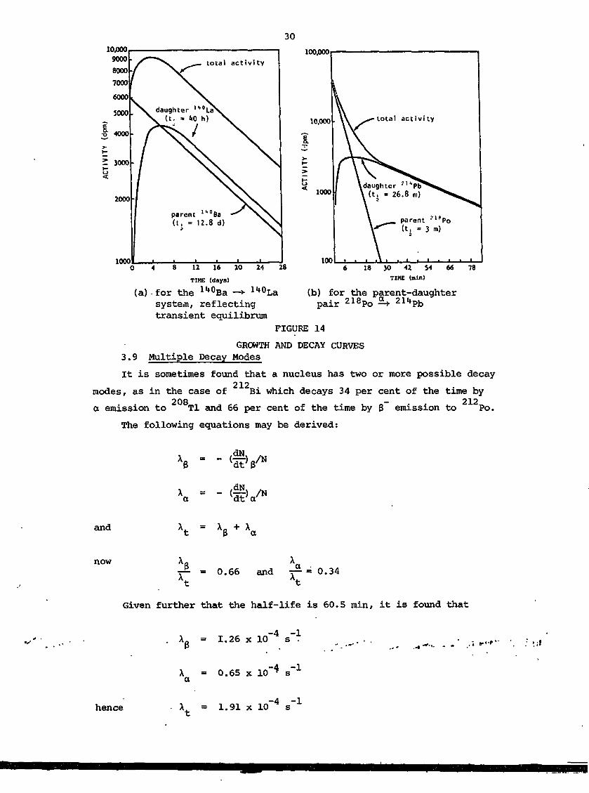
(a).for the llt0Ba —*• llt0La (b) for the parent-daughter
IS 30 42 54 66 78
1000
system, reflectingtransient equilibrium
pair 218Po 21kPb
FIGURE 14
GROWTH AND DECAY CURVES3.9 Multiple Decay Modes
It is sometimes found that a nucleus has two or more possible decay212modes, as in the case of Bi which decays 34 per cent of the time by
a emission to Tl and 66 per cent of the time by $ emission to Po.
The following equations may be derived:
and xt -
now^ - 0.66 and ?=• - 0.34At At
Given further that the half-life is 60.5 min, it is found that
1.26 x 10~4 s'1
X - 0.65 x 10~* s'1a
hence = 1.91 x 10~4 s"1

31
No matter whether the detector detects a-particles only, B-particles
only, or a combination of each, a plot of log (activity) against time
always gives the same period (0.693/X ) = 60 min. The period (0.693/X )
= 173 min is the fictitious period that we would observe if the 8 decay
could be prevented; this is impossible.
3.10 Natural Decay Series
Three complex decay chains occur in nattire for elements of Z > 82
and a fourth (neptunium) has been made artificially. In these, heavy
nuclei emit a-particles and B-particles successively until they achieve
stability as lead or thallium. The existence of four (and only four)
families is a simple consequence of the fact that only a decay (reducing
mass number by 4) and 8 decay (no change in mass number) occur between
these elements. To classify nuclear species by family, the mass number
is divided by 4. This gives the following series:
Mass No.
4n
4n + 1
4n + 2
4n + 3
Name
Thorium
(Neptunium)
Uranium
Actinium
Parent
232.Th
233NP
238u235u
Half-lifeof Parent
,A1010 y
2 x 10⁶ y
4 x 10 y
8 x 10⁸ y
The decay sequence of the 4n + 2 family is shown in figure 15;
There are sometimes two possible decay modes.
2380
4.5 x Iff H a23-.pa
23<H
210po
206pb
210T1
FIGURE 15
THE DECAY SEQUENCE OF THE 4n + 2 FAMILYOF NATURAL RADIOACTIVITIES

32
4. INTERACTION OF RADIATION WITH MATTER
4.1 Alpha-particles
Alpha-particles lose energy by ionising atoms in the matter through
which they travel. The interaction is basically a coulomb interaction
between the positively charged cc-particle and the negatively charged
atomic electrons. The probability of the o-particle interacting with
nuclei is small. Alpha-particles lose energy more rapidly than electrons
because of the low velocity associated with their higher mass (for a
given energy) and because of the double charge. Figure 16 shows the
number of ion pairs/nun along a path as a function of distance in air for
a 5 MeV a-particle. Each ion pair absorbs about 30 eV. As the particle
slows down, the ionisation increases, but may decrease abruptly if the
o-particle collects an electron, effectively decreasing the charge near
the end of its path.
Because of its much larger mass, an a-particle is not appreciably
deflected by collisions* with electrons. Its path is thus mainly straight
until near the end of its path when it moves very slowly and straggling
becomes apparent.
RESIDUAL RANGE(o-PARTICLE), air-cm
FIGURE 16NUMBER OF ION PAIRS PER UNIT PATH FOR ASINGLE PROTON AND A SINGLE ALPHA PARTICLEAS A FUNCTION OF RESIDUAL RANGE. The •residual range is the distance left totravel until the particle comes to rest.The horizontal scale is such that on theleft part of the diagram both particleshave similar speeds. The proton rangethen is 0.2 air-cm shorter than the alpha-particle range.
The:'ionisation process is to some extent statistical. If the
number of particles with range greater than a certain value is plotted,
there is a sudden decrease at the end of the range. Figure 17 shows the
integral and differential range curves, where X is the mean range andMX is the extrapolated range.

33
INTENSITY(A)
c« -onDistanceor Mean Rant*
X«
DISTANCE
NUMBER OF PARTICLESSTOPPED IN A GIVEN DISTANCE
ExtrapolaMdRant* x
(B)
DISTANCE
FIGURE 17
INTEGRAL AND DIFFERENTIALRANGE CURVES
The following table gives an approximate mean range in air for
ct-particles:
Energy
MeV
0
2
5
10
Mean Range in Air
mm
0
10
35
105
-2mg cm
0
1.3
4.5
13.6
The a-particle range in other materials is given by
R « A /p
i.e. 0.00032.air
where A = atomic number. The small range of a-particles means that the
windows of a-particle detectors must be very thin to avoid a substantial
degradation of energy or even total absorption of a-particles.
34
4.2 Beta-particles
The B-particle is identical to the atomic electron, it is light
(mass =0.51 MeV) and has a single charge ± e. The spectrum of 3
energies and the accompanying neutrino emission have been discussed in
sections 3.1 and 3.2 and shown in figures 5 and 6. All 0 active nuclides
have approximately similar spectra.
Since 3-particles are light and consequently fast (for a given
energy) singly charged particles, their specific ionisation is low. In
air, the specific ionisation of fast g-particles is about 40 ion pairs
per centimetre - which is 1/1000 of that for a-particles. This means
that a 3 McV $-particle would have a range in air of over 1000 cm.
However, because the basic interaction is a collision of electron with
electron, the g-particle can be scattered through large angles at each
collision. The 3-particle path is tortuous and there is no well defined
range, but there is a maximum range.
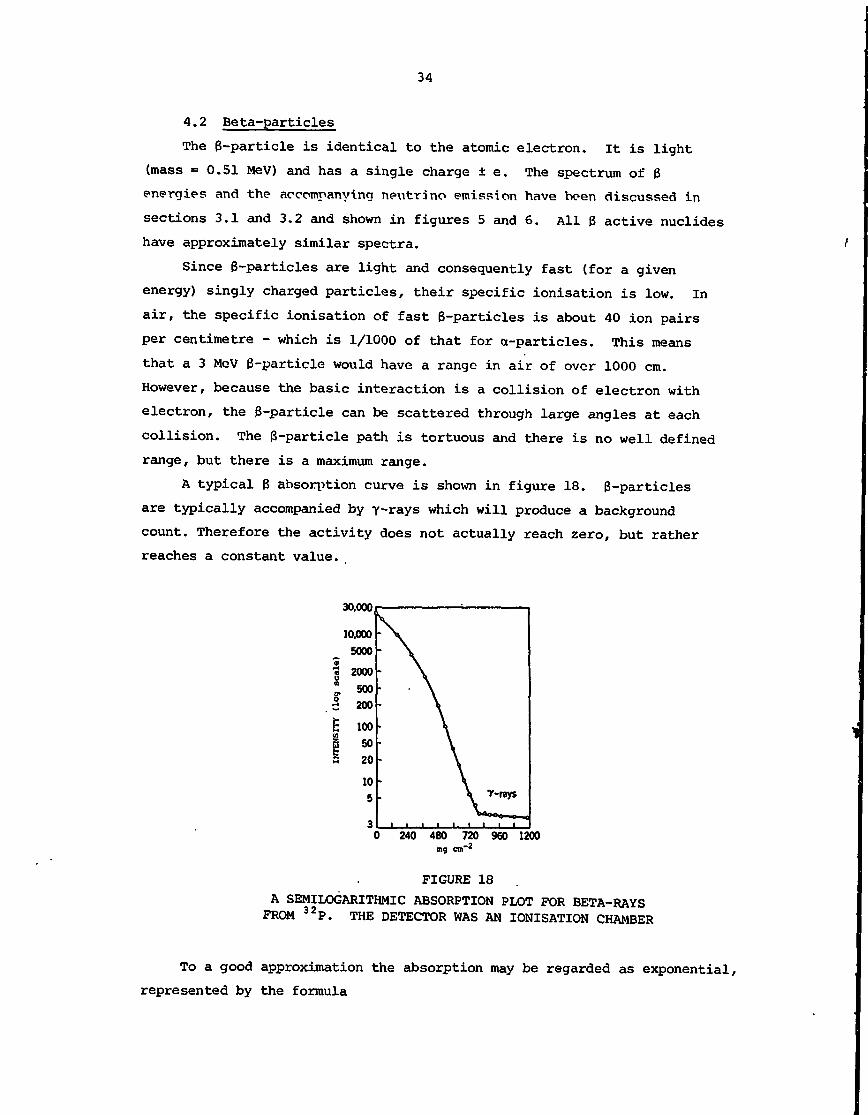
A typical 3 absorption curve is shown in figure 18. 3-particles
are typically accompanied by y-rays which will produce a background
count. Therefore the activity does not actually reach zero, but rather
reaches a constant value.
30.000,
10.0005000
2000500200
10°5020
105
0 240 480 720 960 1200mg cm"
FIGURE 18
A SEMILOGARITHMIC ABSORPTION PLOT FOR BETA-RAYSFROM 32P. THE DETECTOR WAS AN IONISATION CHAMBER
To a good approximation the absorption may be regarded as exponential,
represented by the formula

35
A(x) A eo-yx
where A is the initial activity, A(x) is the activity for absorber
thickness x, and y is known as the absorption coefficient.
Near its end, the absorption curve deviates from the exponential
form. The point at which the curve meets background is called the range
RQ of the (3-particles. The exponential form of the curve is accidental,Psince it also includes the effects of the continuous energy distribution
of the (J-particles and of the scattering of the particles by the absorber.
Thicknesses in absorption measurements are often given in units of
milligrams per square centimetre of absorber. It is found that if the
amount of absorber is expressed as the product of the density and thickness,
the range is nearly independent of the nature of the absorber. The
ability of an element to stop -particles depends on the ratio of atomic
number to mass number, Z/A, which is almost constant for most materials
except hydrogen.
The maximum range of 3-particles
Max. Energy
MeV
0
0..1
0.5
1.0
2.0
5.0
Max. Range
-2mg cm
0
13
180
400
1000
2700
mm Aluminium
0
0.05
0.7
1.5
3.7
10.0
Beta-particles emitted by a sample may be absorbed in the sample.
Low energy betas are stopped by relatively thin layers of material and
self-absorption corrections may be large when dealing with soft beta14emitters such as C. The apparent activity (A) is given by
where
yx
A is the true activity, y is the absorption coefficient,
and x is the thickness of the source.

36
For high energy 3-particles, an additional mechanism for energy
loss must be considered. When an electron passes through the electric
(coulomb) field of the nucleus, it loses energy by radiation. This
energy appears as a continuous X-ray spectrum called brcmsstFalil'Uiig or
bvak-ina vadiat'ian. The energy loss per unit length due to this radiation
is given by:
where N is the number of nuclei cm .
The effect is important at high energies and for materials of high
Z. The ratio of loss by radiation to loss by ionisation is given by:
dx / , „„rad EZ/dE\ 800\dx/. .
lonis
The absorption of positrons is essentially similar to that of electrons,
except that when the positron is stopped it combines with a local atomic
electron and they undergo mutual annihilation. The rest masses appear
as annihilation radiation, two electromagnetic quanta, each having an
energy of 0.51 MeV and going in an opposite direction. This is the
reverse of pair production which is discussed in section 4.3.
4.3 Gamma-rays
Gamma- rays are electromagnetic radiation as are X-rays, light,
radio waves, etc; since they are uncharged, they are very penetrating.
It is not feasible to assign a range to y-rays as may be done with
alphas and betas, but it is practicable to measure the thickness of
absorber required t<~ remove half of the initial Y~*ays from a beam.
Whereas charged particles lose energy by repeated collisions, causing
ionisation losses, yrays lose all their energy in a few interactions.
The intensity (I) of a beam of y~rays decreases exponentially with
the distance of penetration (x) of an absorber:
dx
where the constant of proportionality (y) is the absorption coefficient
where I is the initial intensity.

37
The absorption law is analogous to the radioactive decay law and we
can define a characteristic half thickness (x, ):
x = 0.693/y
There are three main processes involved in the interaction of y
I'dys with liicittci'. Tlicsc cure:
(i) Photoelectric effect,
(ii) Compton scattering,
(iii) Pair production.
An absorption coefficient is defined for each process and the total
absorption coefficient is given by
y = y + y + ype cs pp
The relative probabilities of the processes occurring depend on y-ray
energy and on the atomic number of the absorber.
(i) Photoelectric effect
In this process the photon interacts with the whole atom ejecting
an electron from an inner shell, usually the K-shell. All of the y~ray
energy is given to the electron. The photoelectric effect is the dominant
process at low y-ray energies. The energy of the ejected electron, the
photo-electron, is given by
Ee = EY - EB.E.
Where E_ is the electronic binding energy of the ejected electron.£*£•
For K-shell electrons in aluminium, E_ =1.6 keV, and for lead it iso« E»
88 keV.
The probability of photoelectric absorption decreases with increasing
energy, roughly as
V * 1/EY
Exceptions to this general rule occur when the y-ray energy becomes
sufficient to eject electrons from a more tightly bound shell. For
example, the absorption coefficient for lead has a 5.6 fold increase
when the gamma energy exceeds the K-shell absorption edge at 88 keV.
A careful selection of these edges can be used to filter a narrow band
of Y~raY energies.
The probability of photoelectric absorption increases rapidly with
increasing atomic number, roughly as the fourth or fifth power of Z.
Hence lead is much more efficient as a Y-ray shield than aluminium, at
least at energies below a few MeV.

38
(ii) Compton scattering
At higher y-rays energies, the y-ray may interact directly with an
atomic electron, rather than with the whole atom. Upon interaction, the
y-ray gives part of its energy to an electron which recoils; the y-ray
is then scattered as shown in figure 19. The interaction is elastic
scattering, like snooker balls, with conservation of energy and momentum.
"Y
FIGURE 19
COMPTON SCATTERING
From the conservation of energy and momentum it can be shown that the
scattered photon has an energy
V 1 -I- a (1 - cos 0) Ey
and the Compton electron has an energy
= g(l - cos 0)CE 1 + a(l - cos 0) y
where a = E../m c « 2 E (since m e * 0.5 MeV)
The maximum y-ray energy loss occurs for backward scattering (0 - 180°)
when e 'Y ~ U + 2a)E » h if 4E » 1

39
More accurate calculations show that
E ' =0.22 MeV for E = 2 MeV
= 0.20 MeV f or E 1 MeV
= 0.17 MeV for E =0.5 MeV
Thus the backward scattered Y~rays always have an energy around 0.2 MeV.
The absorption coefficient increases with atomic number because it
depends on the number of electrons encountered. Thus if thicknesses are_2
measured in mg cm , the absorption is independent of the material
(except for hydrogen). The absorption coefficient for the Compton
effect decreases with increasing Y~ray energy. The scattered Y~ray can
undergo a second scattering, or photoelectric or pair production loss,
(iii) Pair production
A high energy y-xay in the strong coulomb field of a nucleus may be
converted to a pair of electrons, one positive and one negative. Since
production of each electron requires 0.51 MeV, according to the equation2
E = me , the minimum energy required of the Y~ray for pair production is
1.02 MeV. As the y-n:ay energy increases beyond 1.02 MeV, the probability
of pair production increases. Gamma-ray energy in excess of 1.02 MeV is
carried away by the pair as kinetic energy which is not necessarily
equally divided. The positron and electron cause ionisation, as discussed
in section 4.2. The positron eventually interacts with another electron
and the two disappear with the formation of annihilation radiation - two
orthogonal Y~rays, each of 0.51 MeV. This is the reverse of pair production.
The probability of interaction by pair production is proportional
to Z and rises sharply with increasing energies.
Relative importance of photoelectric effect, Compton scattering
and pair production in Y~ray absorption
It is obvious from the above that all three processes can occur
(assuming E > 1.02 MeV), but their relative importance varies widely
with energy and with Z. For Y~*ays below 60 keV in aluminium and 600
kev in lead, photoelectric effect is the predominant process. Compton
effect then becomes predominant up to 15 MeV in aluminium and 5 MeV in
lead. At higher energies pair production predominates. Curves showing
the three processes for lead and for aluminium are shown in figure 20.

40
03
0.1
003
001
0.003
0.001
ALUMINUM
p 12.70 g/cm>
0.1 03 I 3 10 30 100 0.1
0.03
.003
.00
FIGURE 20
THE MASS ABSORPTION COEFFICIENTS FOR ALUMINIUM AND LEADAS A FUNCTION OF GAMMA ENERGY IN UNITS OF TOO c2, i.e.
UNITS OF 0.511 MeV (After Ajzenberg-Selove 1960, p.224)
10
5
1
0-5
0-1
005
0-01001 005 0-1 0-5 1
ENERGY (MeV)
5 10 50 100
FIGURE 21
THE GAMMA-RAY ABSORPTION COEFFICIENT FOR VARIOUSELEMENTS (After Cember 1969, p.126).

41
Figure 21 shows the absorption coefficients for the elements lead,
copper, aluminium and carbon for a range of y-ray energies.
Gamma-ray interaction in a detector
The three y-ray absorption processes can occur in a detector and
they produce characteristic distributions in the energy spectra. The
output from scintillation counters and solid state detectors is proportional
to the energy actually deposited in the detector.
Low energy y-rays interact predominantly by the photoelectric
effect and all of the y-ray energy is absorbed. The photoelectrons and
X-rays have only a short range and are usually totally absorbed in the
detector. Hence the photoelectric effect usually gives an output corres-
ponding to the total energy of the incident y-ray, producing the 'photopeak'
in the energy spectrum.
A Compton interaction in the detector produces both a Compton
electron and a scattered y-ray. The Compton electron has a short range
and is usually absorbed in the detector. The scattered y-ray is more
penetrating and often escapes. The energy deposited in the detector is
the incident energy less the energy of the escaped y-ray. The lowest
energy for tho scattered y-ray is about 0.2 MeV for back scattering.
Hence the Compton effect produces a continuous distribution of energies
from zero to E - 0.2 MeV. The Compton effect also contributes to the
photopeak if the scattered y-ray is absorbed in a further interaction.
If pair production occurs in the detector, the kinetic energy of
the electron-positron pair is usually absorbed in the detector. However
1.02 MeV of the energy appears as the two 0.51 MeV annihilation y-rays
which are produced when the positron combines with an electron: Either
or both of these annihilation y-rays can escape from the detector
producing 'escape' peaks at E - 0.51 MeV and E - 1.02 MeV. Of course
if both annihilation y-rays are absorbed in the detector the event will
contribute to the photopeak.
A backscatter peak at about 0.2 MeV is produced by photons which
have been scattered into the detector from the surrounding material.
4.4 Neutrons
Neutrons have no charge and they are very penetrating. Neutrons
only interact with the nuclei of the matter through which they pass,
they do not interact with electrons. The most common interactions, are
elastic scattering, inelastic scattering, capture, and fission [Curtiss 1959].

42
Capture and inelastic scatter are followed by the emission of y-rays,
or other particles.
Neutrons with energies greater than about 1 MeV are called fast
neutrons. Isotopic sources and fission produce fast neutrons of 1 to 10
MeV while DT sources produce fast neutrons of 14 MeV by fusion. The
dominant interaction of fast neutrons in matter is elastic scattering
which slows down the neutron. The mean energy loss in elastic scattering
is
= «.n -=• 2/3
where EI, E are the energies before and after the collision and A is
the mass number of the nucleus. The value of 5 varies from 1.0 for
hydrogen to 0.12 for oxygen and 0.035 for iron to even smaller numbers
for heavier elements [Curtiss 1959].
Elastic scattering reduces the energy of the neutrons until their
energy distribution is the same as the kinetic energy distribution of
gas molecules in the environment, i.e. a Maxwell-Boltzmann distribution.
At a temperature of 20°C the most probable energy is 0.025 eV. Neutrons
with this distribution are called thermal neutrons. The mean number of
collisions to thermalise a fast neutron is 18 for hydrogen, 150 for
oxygen and 520 for iron. Hydrogen is by far the most effective slowing
down medium and the net distance travelled by a 2 MeV neutron slowing
down to thermal energies in water is only 56 mm.
Neutrons at intermediate energies are called epithermal neutrons,
but there is no clearly defined boundary between epithermal neutrons and
either fast or thermal neutrons.
Inelastic scattering of neutrons can occur but it is important only
for fast neutrons. In inelastic scattering, a large part of the neutron
kinetic energy is absorbed by the nucleus which is left in an excited
state and subsequently decays by emitting a characteristic y-xay.
Neutron absorption or capture occurs at all energies but the probability
is much higher at low neutron energies. Below about 1 eV, the absorption
cross section of most nuclei is inversely proportional to the neutron
velocity. The cross section for the absorption of thermal neutrons
varies from 0.2 mbarns for oxygen and 0.33 barns for hydrogen to 2450
barns for cadmium and 46 000 barns for gadolinium. Thermal neutrons
diffuse through matter until they are absorbed. The diffusion length is
28 mm for H O and 540 mm for carbon.

43
Neutron absorption produces the next isotope of the same element in
an excited state, which then decays to the ground state by the emission
of a Y~raY« In a few cases particles are also emitted, e.g. the capture
of a neutron by boron-10 produces boron-11 which decays to lithium-7 and
an a-particle.
Neutron capture causes fission in a few nuclei. Uranium-235 is the
only naturally occurring nuclide which can be fissicned by thcnaal
neutrons. A nucleus of uranium-235 that has captured a thermal neutron
has an 84 per cent probability of fissioning and a 16 per cent probability
of decaying by y-ray emission to a ground state of uranium-236. Fast
neutrons can also cause fission of uranium-238.
5. NUCLEAR REACTIONS
5.1 Reaction Mechanism
It has been shown that charged particles and y~rays lose energy
primarily by interaction with the atom as a whole, whereas neutrons only
interact with the nucleus. In all cases, there is a finite probability
that the incident particle or y ay will collide with the nuclei in the
target material. If the projectile penetrates the coulomb barrier, it
can become lodged in the nucleus, giving both its kinetic energy and
binding energy to the nucleus. The compound nucleus formed is in an
excited state and the excess energy is subsequently lost by processes
involving particle emission, electromagnetic radiation, or fission.
The compound nucleus generally has a lifetime ~ 10 s, which is
long compared with the time taken for nucleons to traverse the nucleus,-22 -21i.e. ~ 10 s. After about 10 s, the compound nucleus has effectively
'forgotten1 how it was formed, so its mode of decay is independent of
its mode of formation.
If the incident particle has a high enough energy, it might not
form a compound nucleus, but instead interact briefly with only a few of
the outer nucleons. This is known as a direct reaction.
A compound nucleus x-aaction may be written
7 1 8 * 4 4Li + Jtt »• °Be >• *He + JJHe '
where the * indicates the compound nucleus formed in an excited state.
Usually the compound nucleus term is omitted. A shortened form of this7 4reaction is Li (p,o) He or, in general terms, X(x,y)Y. Examples of
various types of reactions are (n,y), (n,p) , (n,2n), (p,o), (y,11), etc.

44
27If we consider the compound nucleus Al*, it may be formed in a
number of ways and then decay independently in a number of ways, subject
to the conservation laws of charge and mass energy
23Na + a
25Mg + d-
26Mg
27Al -f
26Al + n
Na -f a
Mg + d
Mg + p
Al +
26Al + n
If the emitted particle is of the same type as the incident particle,
the process is referred to as scattering - elastic if there is no energy
loss and inelastic if there is. Inelastic scattering is accompanied by
y-ray emission as the excited residual nucleus returns to a stable
ground state configuration.
The nuclear potential (coulomb) barrier plays an important part in
nuclear reactions. It repels charged particles and the height of the
barrier is greater for high Z and multiple-charged particles. Charged
particles of sufficient energy to overcome the barrier can be obtained
from accelerators. For uncharged particles there is no potential barrier
and the probability of capture is enhanced.
Uncharged particles are more likely to be emitted than charged ones
because emitted particles must also overcome the potential barrier.
There is a finite probability that a charged particle can escape without
surmounting the potential barrier by a process known as 'tunnelling1.
5.2 Energy Considerations
In a reaction X(a,b)Y, the net change in energy, the Q value, is
given by:2
Q = c [rest mass of nuclides before reaction-
rest mass of nuclides after reaction]
2
In computing the reaction Q value, the mass of the neutral atom is used.

45
Q may be either positive or negative. If it is positive, the
reaction is exothermic and the reaction will proceed with the release of
energy. Most of this energy appears as kinetic energy of the emitted
particle, but some appears as recoil energy of the residual nucleus. If
Q is negative, the reaction will not proceed unless the available kinetic
energy of the incident projectile is greater than the threshold energy,
aiven bv
E,, = -
where the correction (m - m / m ) converts the kinetic energy to centre-X cl X
of-mass energy.
14 4 17 1 14 17Example 1 _N + He »• 0 + H or N(a,p) 0
The rest mass of the nuclides before reaction is
M(14N)
M(4He)
14.003074 a.m.u.
4.002603 a.m.u.
Total 18.00567 a.m.u.
and the rest mass of the product nuclides is
M(170)
1
Total
= 16.999131 a.m.u.
1.007825 a.m.u.
18.006956 a.m.u.
Hence = -0.001279 a.m.u.
= -1.19 MeV
This means that the a-particle must provide energy for the reaction to
occur and, to allow for recoil energy, the threshold energy for the
a-particle is:
„ 14 + 4Eth - 14
1.5 MeV
Example 2 Li or Li (p,a)a

46
The rest mass of the initial nuclides is
M(7Li) = 7.016005 a.m.u.
M(1H) = JLOCV7B25 a.m.u.
Total 8.023830 a.m.u.
and the rest mass of the final two a-particles is
2 x M(4He) = 8.005207 a.m.u.
Hence Q = + 0.01862 a.m.u.
= 17.3 MeV
The reaction is exothermic and the 17.3 MeV will appear as kinetic
energy of the two resultant a-particles.
5.3 Reaction Probability
The probability that a particular reaction will take place depends
on the nuclear properties of the target nucleus, the type of incident
particle, the number of target nuclei and the number of incident particles.
All of the nuclear properties are combined into one parameter, called
the cross section and given the symbol 0.-2
Suppose a parallel beam of n particles m impinges on a target of
thickness dx containing N nuclei m . Then the number of reactions_2
R m will be
R = nNadx
The cross section is the probability of interaction per nucleus per
incident particle. It has dimensions of area and, because it rypically_ oc «.*3O O
has values of 10 to 10 m , it is usually expressed in units of-24 2 -28 2 2barns, where 1 barn =10 cm = 10 m = 100 fm . The cross section
can be thought of as the effective area of a nucleus through which an
incident particle must pass for the reaction to occur.
Each interaction has its own cross section which varies as a function
of energy. If there are several modes of decay, each mode has its own
partial cross section and the total cross section is the sum of all the
partial cross sections. At some energies, there are sharp increases in
the cross section, called resonances. The size and energy of the resonances
depend on the energy levels of the target nuclide and the compound
nucleus.

47
Cross sections vary over many orders of magnitude. The thermal
neutron capture cross sections vary from 2.6 x 10 barns for Xe to
0.18 mbarns for 0. The cross sections for charged particle reactions
can be much smaller. The angular distribution of emitted particles is
important for some applications; this is given as the differential
cross section, da/dfl, which is the cross section per un.it solid angle as
a function of the angle of the emission.
There are extensive tabulations of cross sections in the serial
publication Nuclear Data Tables.
5.4 Radionuclide Production
Most radionuclide production is carried out in the high neutron
fluxes of reactors. Generally, neutron- induced reactions produce neutron-
rich nuclides which decay by 3 decay.
(a) Slow neutrons
59Co(n,Y)6°Co a = 37 b t, = 5.26 y
75As(n,y)76As a = 4.4 b t - 26.3 h
Cobalt-60 is one of the most widely used of all radioisotopes:
14N(n,p)14C 0 = 1.8 b t = 5730 y
35Cl(n,p)35S a = 0.5 b t, = 87.2 d
In the (n,y) reaction the parent always dilutes the daughter product
(not carrier free). In (n,p) reactions chemical separation gives carrier
free material.
(b) Fast neutrons
32S (n,p)32p t = 14.3 d
6Li(n,a)3H t, = 12.3 y
40Ca(n,a)37Ar T = 34.8 d
These reactions yield carrier free material, although other reactions
may occur to a lesser extent.
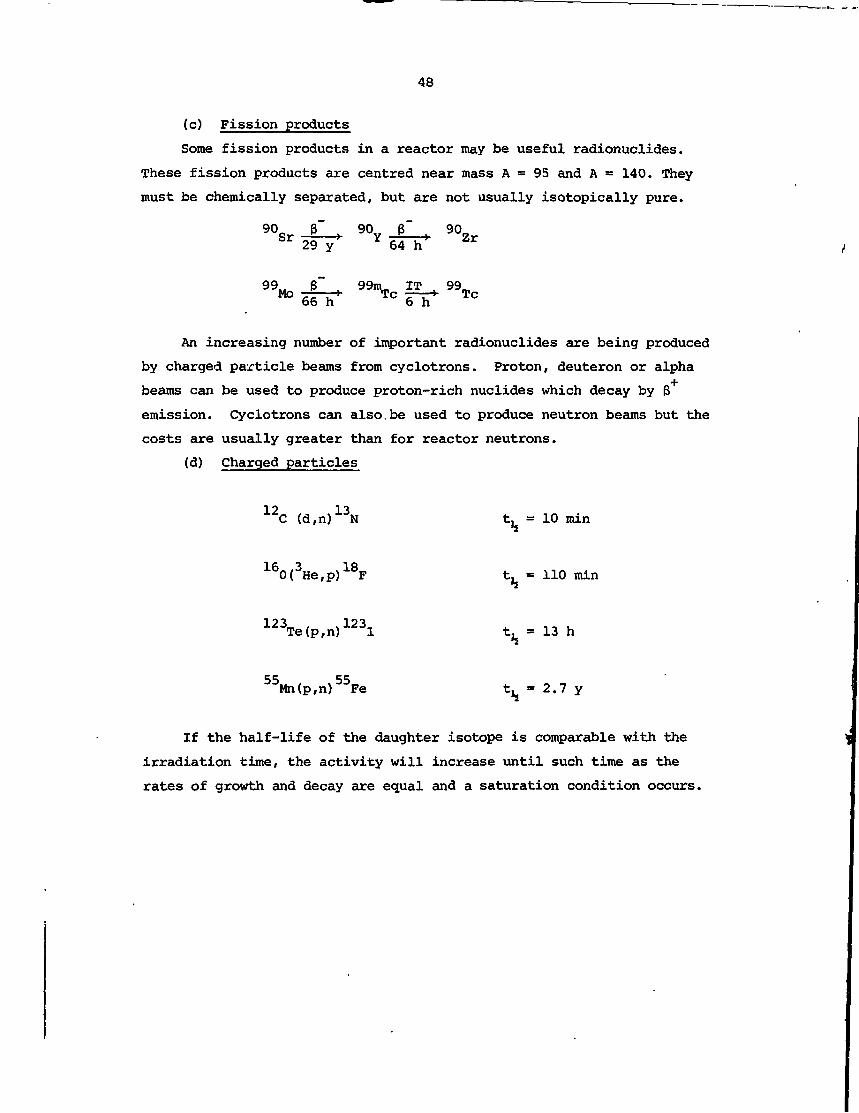
48
(c) Fission products
Some fission products in a reactor may be useful radionuclides.
These fission products are centred near mass A = 95 and A = 140. They
must be chemically separated, but are not usually isotopically pure.
90_ BSr 29T9"
99M B~Mo - .. . >66 h
9°YJ* 902r64 h
99mm IT 99mrp^i «_^_««^. *T*f^1C 6 h r°
An increasing number of important radionuclides are being produced
by charged particle beams from cyclotrons. Proton, deuteron or alpha
beams can be used to produce proton-rich nuclides which decay by B
emission. Cyclotrons can also.be used to produce neutron beams but the
costs are usually greater than for reactor neutrons,
(d) Charged particles
12C (d,n)13N tj = 10 min
160(3He,p)18F t, = 110 min
123Te(p,n)123l t = 13 h
55Mn(p,n)55Fe t,= 2.7 y
If the half-life of the daughter isotope is comparable with the
irradiation time, the activity will increase until such time as the
rates of growth and decay are equal and a saturation condition occurs.

49
6. BIBLIOGRAPHY
Ajzenberg-Selove, F. [I960]- Nuclear Spectroscopy. Part A. Academic
Press, New York.
Cembor, H. [1969]- Introduction to Health Physics. Pergamon Press,
Oxford, UK.
Curtiss, L.F. [1959]- Introduction to Neutron Physics. D. van Nostrand
Co. Inc., Princeton, New Jersey, Chapter VI.
Evans, R.D. [1955]- The Atomic Nucleus. McGraw-Hill Book Co, Wallingford,
Conn.
Foster, A. and Wright, R.L. [1977]- Basic Nuclear Engineering. Allyn and
Bacon, Inc., Boston, Mass.
Jakeman, D. [1966]- Physics of Nuclear Reactors. The English Universities
Press Ltd, London.
Lederer, C., Hollander, J.M., and Perlman, I. [1968]- Table of Isotopes,
6th Edition. John Wiley and Sons Inc., New York.
Lederer, C.M. and Shirley, J., (eds.) [1978]- Table of Isotopes.'7th
Edition. John Wiley and Sons, Inc., New York.
Rollo, F.D. [1977]- Nuclear Medicine Physics, Instrumentation and
Agents. C.V. Mosby Co., St. Louis.
Segre, E. [1976]- Nuclei and Particles. W.A. Benjamin, Inc., New York.

51
CHAPTER 2
THE DETECTION AND MEASUREMENT OF
NUCLEAR RADIATION
A Series of Lectures
E.M. Lawson
P.L. Eisler

53
PART A
RADIATION DETECTION AND MEASUREMENT
by
E. M. Lawson

55
1. INTRODUCTION
The fundamental mechanism for the operation of a radiation detector
is dissipation of the energy of a charged particle in a suitable medium.
We can think of a radiation detector as an energy transducer. The
energy is usually converted into an electrical signal - charge, current
or voltage. The. medium from which a detector is made can be solid,
liquid or gas. The charged particle may be primary radiation, or it may
result from the interaction of neutral primary radiation with the material
of the detector (e.g. an electron from a Y~ray interaction, an alpha
particle from a neutron interaction).
Useful energy dissipation is principally by two processes: ionis-
ation and scintillation. In the general ionisation process, electrons
are removed from neutral atoms to form a negative electron-positive ion
pair. However, in a semiconductor, negative electrons and positive
holes (with approximately equal masses) are produced. The positive and
negative charges are separated and collected using an electric field
which must be supplied. In the scintillation process, the atoms of the
medium are excited; light is emitted when de-excitation occurs. The
light is collected by means of reflectors. It should be noted that, in
a scintillator, both energy loss processes occur at once but only one is
actually used. Other forms of energy dissipation are molecular dissoci-
ation, bremsstrahlung, Cerenkov and synchrotron radiation.
Types of Detector
lonisation
Gaseous detectors - ionisation chamber,
proportional counter, Geiger-Mueller (GM)
counter. Semiconductor detector.
Scintillation
scintillation counter
phosphors e.g. ZnS screen
A certain amount of energy is required to produce an electron/
positive ion pair in a medium. This ionisation energy (to) is different
from one material to another but it is approximately 30 eV in most
gases. It is to be noted that the ionisation energy is independent of
type (i.e. Z and M) of the incident energetic charged particle.
Two fundamental modes of operation can be distinguished. Firstly,
a pulse counting system in which each event is recorded and secondly, a
mean current system in which the net effect of all events is measured.

56
The mean current mode is applicable where the events are so frequent
that separation in time is not practicable. It has the advantage of
simpler associated equipment. The signals in both operating modes are
usually very small and require amplification.
2. ELECTROSTATICS OF PULSE FORMATION FOR THE IONISATION CHAMBER
Consider figure 1 which shows diagrammatically a simple parallel
plate counter. We wish to calculate the induced charge on the electrode
system due to the motion of an electron/positive ion pair in the col-
lecting field. The two are initially in close proximity and there is no
external effect. As the field separates the charges, work is done on
them which must result in a change in the potential energy of the capac-
itor C formed by the electrodes. The equilibrium potential energy is
CV0/2.
-5-Vo
FIGURE 1
The induced charge due to this movement results in a change in
potential from V to V + 6V, where 5V is small and equal to 6q/C (Sq
is the induced charge as distinct from the static charge Q
Therefore,
change in potential energy = -^ \(VQ + 6V)2 - VQ
2
r x 6q
cvo).
C x V x 5Vo
When these charges are separated by a potential difference, V, the
work done is V x e, where e is the electron charge. The change in
potential energy V x <Sq must be equal to the work done, V x e; there-
fore,
e x or 6V £ Y—C Vo
e_ AXC d
where AX is the distance between the two charges.
(1)
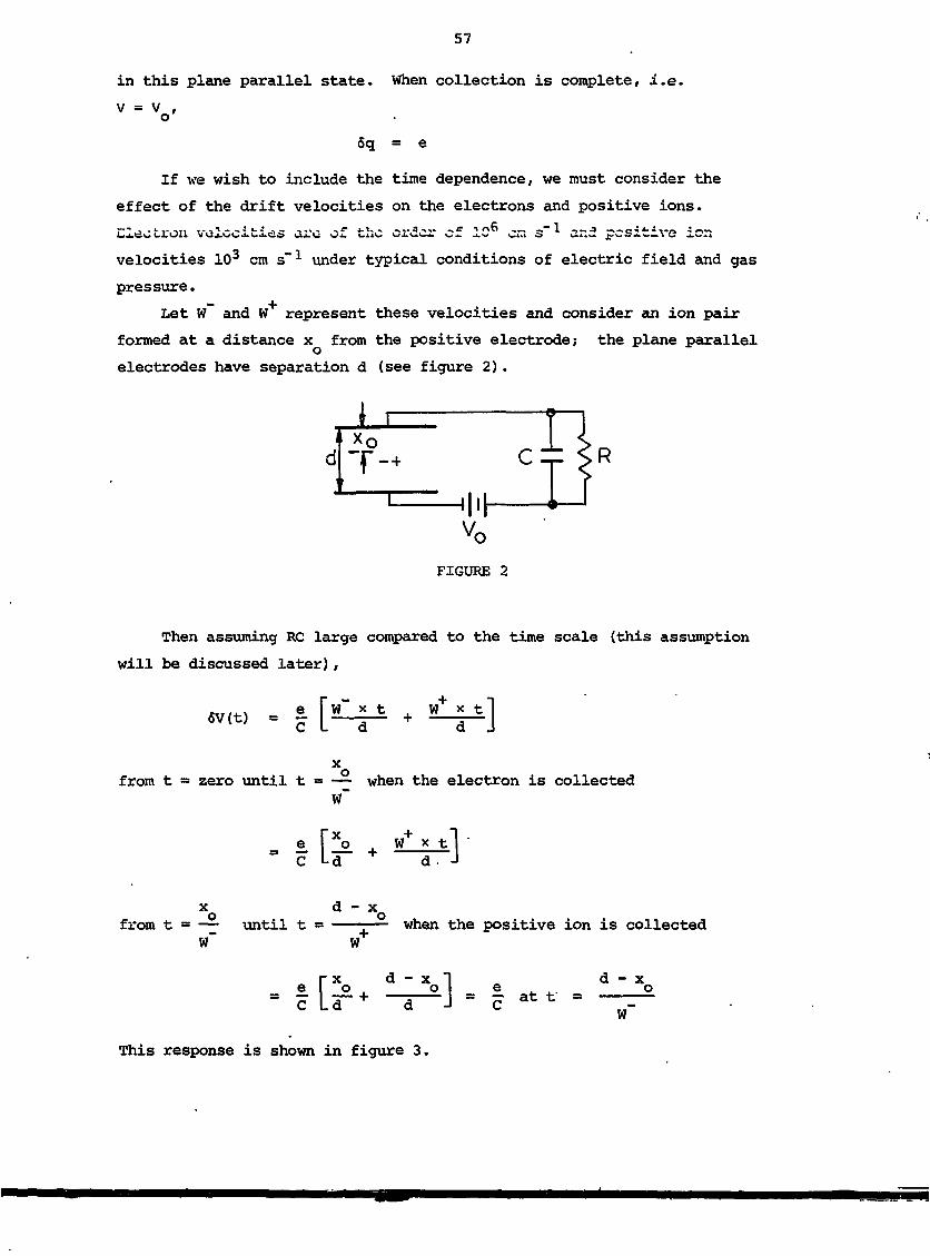
57
in this plane parallel state. When collection is complete, i.e.v = V
6q = e
If we wish to include the time dependence, we must consider the
effect of the drift velocities on the electrons and positive ions.
Electron velocities ore of the order cf 10fi cm s'1 and positive ion
velocities 103 cm s~1 under typical conditions of electric field and gas
pressure.
Let W~ and W represent these velocities and consider an ion pair
formed at a distance x from the positive electrode; the plane parallel
electrodes have separation d (see figure 2).
FIGURE 2
Then assuming RC large compared to the time scale (this assumption
will be discussed later),
wtt)
xfrom t = zero until t = — when the electron is collected
W~
e [Xo .,. W* x tl •c LdT + a. J
xo d " xofrom t = — until t = — when the positive ion is collected
W~ W
e ... d- xo
W
This response is shown in figure 3.
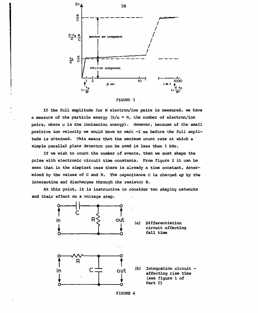
OV^
eC
^!
e
•? c
k 58
4
positi\
1 r\ect
K ion component
,, •
ron rrmmftn 0r\\
/I
(Isec1OOOATd x0
FIGURE 3
If the full amplitude for N electron/ion pairs is measured, we have
a measure of the particle energy (E/w = N, the number of electron/ion
pairs, where o> is the ionisation energy). However, because of the small
positive ion velocity we would have to wait ~1 ms before the full ampli-
tude is attained. This means that the maximum count rate at which a
simple parallel plate detector can be used is less than 1 kHz.
If we wish to count the number of events, then we must shape the
pulse with electronic circuit time constants. From figure 2 it can be
seen that in the simplest case there is already a time constant, deter-
mined by the values of C and R. The capacitance C is charged up by the
interaction and discharges through the resistor R.
At this point, it is instructive to consider two shaping networks
and their effect on a voltage step.
4 't cin
A Dl r>
in
r>
R<
°T
\j
out
out
r>
(a) Differentiationcircuit affectingfall time
(b) Integration circuitaffecting rise time(see figure 1 ofPart C)
FIGURE 4
59
The situation under discussion is like that shown schematically in
figure 4a. If RC is large compared to the positive ion transit time,
the pulse will be as shown in figure 3 with a correspondingly poor count
rate capability. If the value of RC is changed, we can differentiate
the pulse and effectively measure only the electron component to the
induced signal. The count rate .capability is much improved - perhaps 1 MHz.
However, the ability to determine the particle energy is lost since the
electron component is sensitive co position.
This spatial dependence of the electron signal can be reduced,
although not eliminated, by using a coaxial structure. The central
electrode should be positively biased to collect electrons. In this
configuration, the electric field E(r) at a point r from the centre is
VE(r) r x £n (r /r.)o i
where V is the applied potential difference and r and r. are the radii
of the outer and inner electrodes respectively. A large change in
potential difference takes place close to the central electrode (the
anode), so most electrons will experience this potential drop and thus
give a signal which is almost independent of the position of interaction.
Remember that the induced signal depends on potential drop. From
equation 1
V + V+ VSv s= — — = — — _ e
C V C V C Vo o o
because V is very small; V and V are the potential drops associated
with the positive ion and electron respectively.
Alternatively, the spatial dependence of the elec-uron signal can be
eliminated by using a Frisch grid chamber; this is a parallel plate
chamber in which there is a screen or grid of fine wire placed between
the two electrodes. Its potential is intermediate to that of the anode
and cathode. Provided that ionisation only takes place between the
cathode and the grid, a constant signal will be induced by the electrons
when they pass through the grid to the anode. There is no signal in-
duced on the anode until the electrons pass through the grid.
It is useful at this stage to introduce the concept of dead time.
This can be thought of as the minimum time that can elapse between two
interactions if they are to produce two counts. The emission of nuclear
radiation is a random process, and each new event must be considered as

60
independent of any other. Because they are too close together, some
proportion of the events will not be counted, however low the mean count
rate and however short the dead time of the system. Commonly, radiation
measurements are made using detectors and associated electronics that are
capable of far higher mean count rate than that under consideration.
It is possible to correct for the counting losses due to dead time
provided that dead time per pulse can be defined accurately and if the
correction factor is not large. If m is the observed count rate, the
system must have been non-receptive (dead) for a total period of m T
(where T is the dead time per pulse). The actual receptive or 'live'
time is (1 - m T) and the true mean count rate iso
mmt = 1 -m T
3. BIBLIOGRAPHY
Knoll, G.F. [1979] - Radiation Detection and Measurement. John Wiley
& Sons, New York.
Price, W.J. [1964] - Nuclear Radiation Detection. McGraw-Hill, New
York, 2nd edition.
61
PART B
EXAMPLES OF RADIATION DETECTORS
by
E. M. Lawson

63
1. GASEOUS DETECTORS
1.1 lonisation Chambers and Proportional and Geiger-Mueller Counters
The previous lecture dealt mainly with simple ionisation chambers
having plane parallel electrodes. The alternative and more common
geometry is a coaxial structure with the central conductor acting as the
anode. It has been shown that when operated in the pulse mode the
electron signal is less sensitive to position. The inner electrode is
frequently a fine wire of perhaps 0.1 mm diameter.
In theory at least, the operation of the above gaseous detectors
may be illustrated by considering a coaxial device containing a volume
of a gas such as H2, Ar, CHif, Ne, or He and increasing the applied
potential. Two cases corresponding to ionisation by a 3 KeV ex-particle
and a 30 keV (3-particle will be assumed.
Figure 1 shows a plot of N, the number of electrons collected at
the anode, as a function of the applied potential. The behaviour of
this detection system is considered in the following regions of applied
voltage.
4OO 6OO 8OO 1OOO 120O
APPLIED BIAS (V)
FIGURE 1
NUMBER OF ELECTRONS COLLECTED AT THE ANODEAS A FUNCTION OF APPLIED POTENTIAL
Reg-Ion OA: The detector is acting as an ionisation chamber with severe
recombination and has no practical use. Recombination is the reverse of
ionisation, the electron and positive ion combining to form a neutral
atom. It is most severe when the ionisation density is high, i.e. in
the path of fission fragments.
Region AB: This is the region of operation of an ionisation chamber.
Charge collection is complete or saturated. The pulse amplitude is

64
proportional to the energy lost in the chamber by the radiation. As
was mentioned in the previous lecture, the pulse amplitudes are very
small.
The purity of the gas is very important, being typically 1 part in
105. Certain impurities such as oxygen, water vapour and some halogens
have a high electron affinity and must be kept from poisoning the gas.
If an atom or molecule captures an electron and becomes a negative ion,
the associated drifted velocity becomes very small; this is typically
103 cm s""1, which is the same as for positive ions. The probability of
recombination is thereby increased and collection times are increased.
Region BC: The electric field in the vicinity of the wire becomes large
enough for an occasional electron to gain sufficient kinetic energy
between collisions with gas atoms to cause secondary ionisation. This
kinetic energy will exceed the ionisation potential of the gas atoms.
The secondary ionisation constitutes an internal multiplication or
amplification mechanism. The multiplication takes place in the high
field region near the wire with the result that electron 'avalanches'
are quite localised.
Notice that the curves for the two energetic particles are essen-
tially parallel, indicating that the ratio of the number of ion pairs
from the two classes of events is maintained. Towards C, the magnitude
of the pulses from the detector - a proportional counter - may be four
or five orders of magnitude greater than those from the ionisation
chamber. This of course eases the problem of electronic amplification.
For constant internal gain there must be no sharp points on the
anode wire and end effects must be corrected. Distortion of the field
lines will occur at the endi; of the detector unless field tubes are
used. These field tubes are short coaxial electrodes placed at each end
of the detector and held at an equipotential. They remove end effects
and define the sensitive volume. In the plane parallel situation, end
effects can be removed with a guard ring.
Region CD: In this region the internal amplification continues to
increase but the proportionality is lost. As the avalanche size in-
creases, a high density of slow moving positive ions is formed near the
wire. This space charge causes electrostatic screening and produces
large local changes in the electric field near the wire. The onset of
this region depends to some extent on the density of the initial ionis-
ation, i.e. begins sooner for the a-particle. This region of limited
proportionality is of little practical use.

65
Region DE: This is the region of Geiger-Mueller (GM) operation. An
ionising event initiates an electron avalanche as before. However,
because of the higher field, the discharge is so intense that it spreads
or 'burns' along the complete length of the wire, propagated by the
ultraviolet photons produced in the discharge. The same discharge or
signal results whether the initial ionisation is a single electron-ion
pair or a strongly ionising particle.
Because of the intense ionisation and excitation of the gas during
the discharge, it is necessary to 'quench' the discharge to ensure that
the residual effects do not initiate further avalanching. This can be
accomplished by adding a small amount of organic vapour or halogen gas
to the primary filling. The energy of residual ultraviolet photons
(which might initiate another avalanche) is used to dissociate the
organic molecules but is completely absorbed by a halogen molecule. A
further method of quenching is the use of a quenching probe which is an
electronic unit for reducing the applied potential below the threshold
value, thus allowing complete recombination to take place.
Thus within the GM region, all events give rise to a uniform pulse
amplitude which may have a magnitude of several volts and thus require
no further amplification. Energy discrimination is possible for the
ionisation chamber and the proportional counter, but not for the GM
counter.
An important limitation to the use of GM counters is the long dead-
times inherent in this type of detector. In the GM counter, due to
strong screening by positive space charge near the anode and to the slow
removal of this space charge, it is several hundreds of microseconds
before the field has recovered sufficiently to produce a full size
pulse. With a quenching probe, the dead-time may be fixed electron-
ically and thus permit correction of the results. The dead-time is
typically ICf1* to 10"3 s.
The point D, at which time GM operation commences, is called the
threshold voltage and the region DE, the plateau. Important practical
considerations are the length and slope of this plateau since these
indicate the dependence of the results on operating voltage.
2. SCINTILLATION DETECTORS
Gaseous detectors are extensively used to detect particulate
radiation. However, for y-ray detection where cross sections are low
the efficiency of the gaseous detectors is only a few per cent.
Devices for detecting a Y-ray interaction within a solid or liquid

66
wii;. obvious!v be much more efficient. The scintillation counter is in
this class.
Historically, this is one of the earliest detection methods.
Rutherford and his colleagues made many measurements by counting the
scintillations produced on a ZnS screen by a-particles.
The modern scintillation counter combines material which is lumin-
escent under the effect of radiation, and some type of photodetector
such as a photomultiplier. The luminescent medium may be an inorganic
crystal such as Mai or Lil. Activators such as thallium or europium may
be added (0.01%) to increase the probability of luminescent decay.
Other luminescent media are organic crystals such as anthracene, stilbene
and naphthalene, and organic phosphors such as terphenyl dissolved in a
suitable solvent or plastic.
A typical scintillation counter is shown schematically in figure 2.
A charged particle, for example, a secondary electron produced by the
introduction of a y~raY within the crystal, dissipates its energy by
ionisation and excitation.. Most of this energy loss is degraded into
heat but a small fraction results in relatively long-lived, excited
states (lifetimes of 10"9 to 10"6 s). These excited states relax to the
ground state resulting in the emission of visible and ultraviolet photons.
Visible or u.v. photons
Secondaryelectron --
Dynode
Photo-cathode
Scintillator Photomultiplier
FIGURE 2
Shuntcapacitance
SCHEMATIC DIAGRAM OF TYPICALSCINTILLATION COUNTER
The crystal and photomultiplier must be optically coupled and
maintained in a light-tight enclosure. Some of the photons will inter-
act at the photocathode of the photomultiplier producing photoelectrons.

67
The photomultiplier is a vacuum tube constructed with a photocathode/ a
series of 'dynodes' and a collector, each being maintained at progress-
ively higher positive potentials. Materials used for the photocathode
include Ag, Na, K, Sb and Cs and their alloys. The photoelectrons are
accelerated to the first dynode where they collide with a treated sur-
face (e.g. Cs-Sb, Ag, MgO-Cs, Be-Cu) to produce several (typically three
or four) secondary electrons; those arc accelerated to the second
dynode where more secondary emission occurs. The end result of this
electron multiplication is the collection of a large pulse of electrons
at the anode (the collector). This collected charge produces a voltage
pulse across the shunt capacitance of the output. Because of the ampli-
fication this pulse can be quite large. If 6 is the electron gain at
a dynode, the total gain G = 6 , where n is the number of stages. For
example if 6 = 4, .1 = 10, G = 410 = 106.
Several points should be noted:
(i) Good optical coupling is essential (this may necessitate
the use of reflectors, light pipes and wavelength shifters).
(ii) The voltage across the tube will generally be > 700 V with
about 70 - 100 V between dynodes. The gain is a sensitive
function of the voltage and so good quality extra high tension
(EHT) units are required.
(iii) Owing to the short decay times in the scintillator and short
electron transit times in the photomultiplier, short RC time
constants may be used to allow operation at high count rates,
e.g. < 100 kHz.
(iv) The gain of a scintillation detector is temperature dependent,
due mainly to variation in the gain of the photomultiplier -
about -0.3% per °C. Electronic gain stabilisers (discussed in
the following lecture) are usually required to compensate for
this gain change when accurate energy analysis is required.
3. SEMICONDUCTOR DETECTORS
Basically, the semiconductor detector consists of a large, reverse
biased p-n junction diode made from very pure (1 part in lO1^) silicon
or germanium. The depletion region is the sensitive volume of the
detector; its depth depends on the applied voltage and the material
purity. If one side of the junction is heavily doped and the other
lightly doped, the depletion depth occurs in the lightly doped material
and the material on the other side of the junction can be made very thin
to allow the entrance of radiation without much absorption (see figure
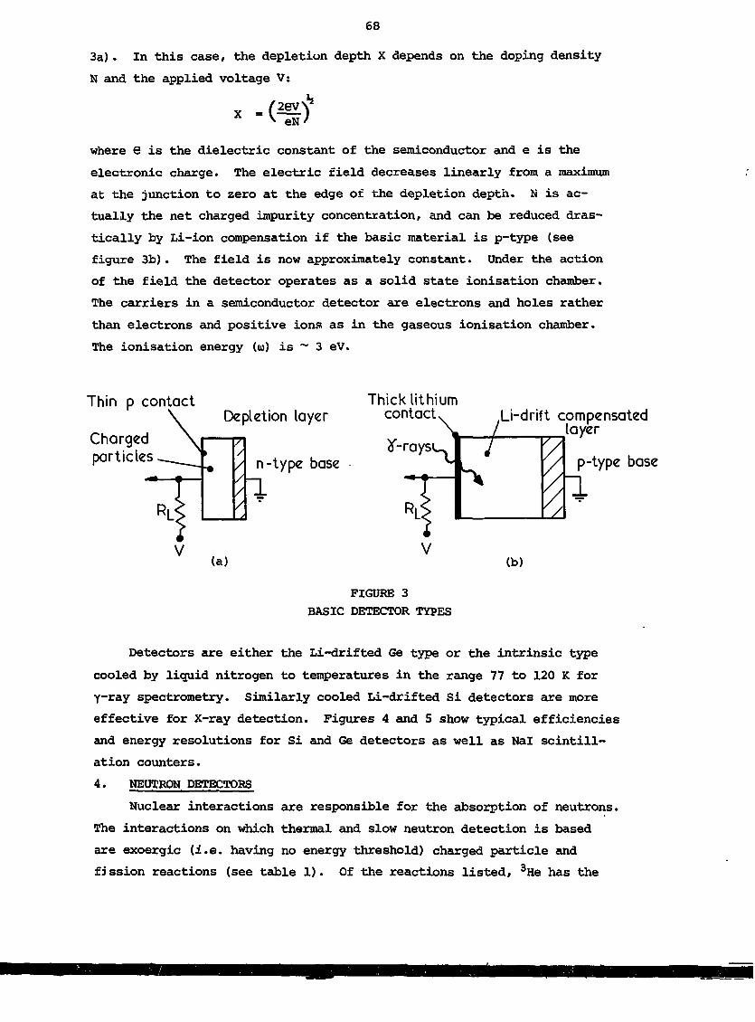
68
3a). In this case, the depletion depth X depends on the doping density
N and the applied voltage V:
* ^tmt\I
X =
where 6 is the dielectric constant of the semiconductor and e is the
electronic charge. The electric field decreases linearly from a maximum
at the junction to zero at the edge of the depletion depth. N is ac-
tually the net charged impurity concentration, and can be reduced dras-
tically by Li-ion compensation if the basic material is p-type (see
figure 3b). The field is now approximately constant. Under the action
of the field the detector operates as a solid state ionisation chamber.
The carriers in a semiconductor detector are electrons and holes rather
than electrons and positive ions as in the gaseous ionisation chamber.
The ionisation energy (u) is ~ 3 eV.
Thin p contact
Chargedparticles
Depletion layer
n-type base
n
Thick lithiumcontact,
*•raysu^
;RI>; ^
FIGURE 3
BASIC DETECTOR TYPES
Li-drift compensatedlayer
p-type base
(b)
Detectors are either the Li-drifted Ge type or the intrinsic type
cooled by liquid nitrogen to temperatures in the range 77 to 120 K for
Y~ray spectrometry. Similarly cooled Li-drifted Si detectors are more
effective for X-ray detection. Figures 4 and 5 show typical efficiencies
and energy resolutions for Si and Ge detectors as well as Nal scintill-
ation counters.
4. NEUTRON DETECTORS
Nuclear interactions are responsible for the absorption of neutrons.
The interactions on which thermal and slow neutron detection is based
are exoergic (i.e. having no energy threshold) charged particle and
fission reactions (see table 1). Of the reactions listed, 3He has the
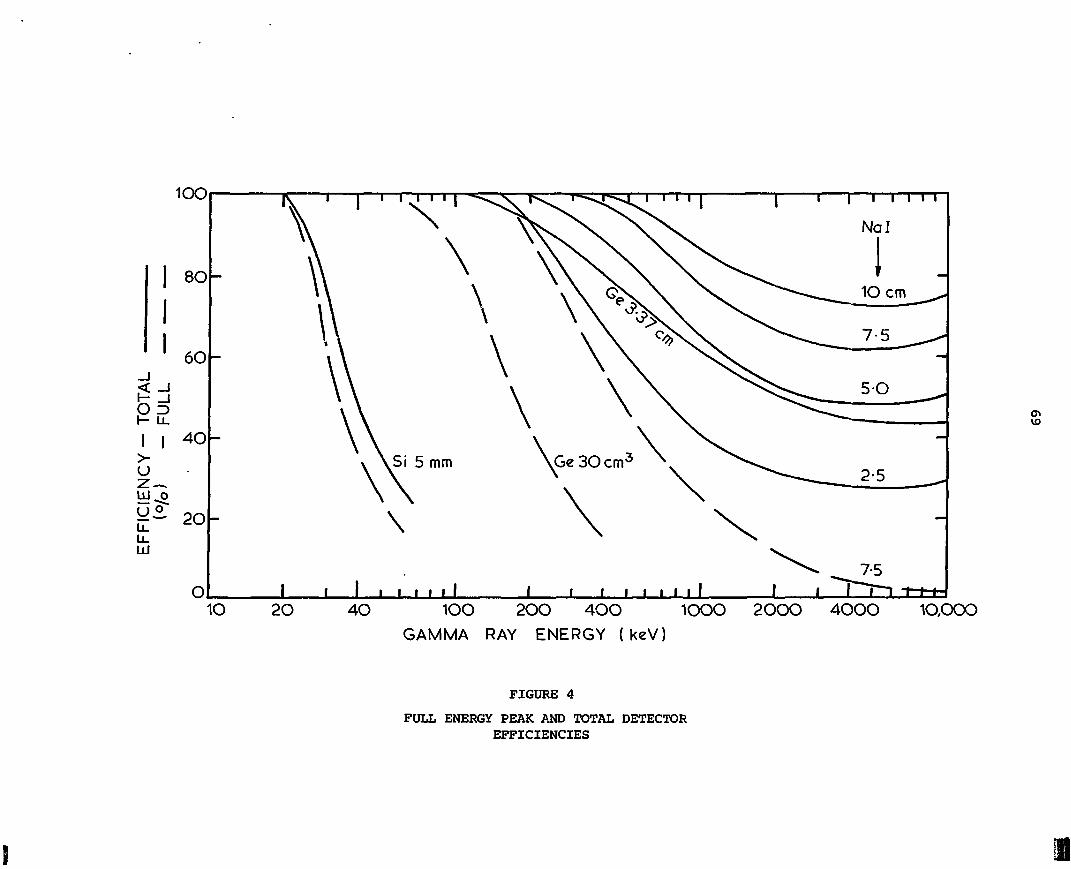
1OO
2O 4O 1OO 2OO 4OO 1OOO
GAMMA RAY ENERGY ( keV)
2OOO 4OOO 1O,OOO
vo
FIGURE 4
FULL ENERGY PEAK AND TOTAL DETECTOREFFICIENCIES

RESOLUTION FWHM
•n
§
OO
O
O73
m om TT
O <
-<
TI nr
i 1 1 1 1 1O7T
OITT
Nal FWHM

/JL
highest cross section (5330 barns) for interaction with a thermal neutron.
In general, thermal neutron cross sections, and hence efficiencies, fall
off to higher energies with a 1/v dependence (v is the neutron velocity).
A neutron counter based on detecting the 0.48 MeV y~ray from the decay
of the Li7 excited state can be made by surrounding a Nal scintillator
with boron.
TABLE 1
NEUTRON DETECTORS
Reaction
n + 10B + 7Li + HHe
»*I°-{&n«K'""
7Li* -»• 7Li + Y
n + 6Li •*• 3H + He
n + 3He •»• 3H + 1H
fission of 233U,
235u, 239pu
Detector Type
BF )3 ( proportional counterB-lined )
Detection of 0.48 MeV y~ ay in Nal
scintillation counter shielded with B
Lil scintillation counter
He proportional counter
lonisation chamber with fissile layer
on inner wall (fission counter)
Fast neutrons are commonly detected by elastic (billiard ball)
scattering on the nuclei (protons) of hydrogen. Liquid and plastic
organic scintillators are commonly used for fast neutron spectroscopy
although efficiencies are low. Provided that they are slowed down
(thermalised) fast neutrons can also be detected by the instruments
listed in table 1.
5. CHOICE OF DETECTOR
Table 2 summarises the instrument used to detect $, X, y
neutrons (n) . In the mineral industry, ionisation chambers are used
mainly in Y~raY density gauges. There is however, a general tendency to
replace these with scintillation detectors which are much more efficient
and hence allow the use of lower activity sources. Use of the GM counter
is now limited to radioactive mineral prospecting and some health physics
instrumentation .

The choice of detector for X- or y-ray measurements depends on
requirements for the detector's efficiency/ sensitive volume, energy
TABLE 2
COMMONLY USED DETECTORS FOR ALPHA- AND BETA-PARTICLES,
GAMMA-RAYS AND NEUTRONS
Detector Type
Gas Detectors
lonisation chamber
Proportional counter
GM counter
Scintillation Counters
Nal crystal
Plastic or liquidscintillator
Semiconductor Detectors
Si
Ge
a, 3
'
X-ray
/
y-ray
'
n
'
resolution, and ratio of full energy peak to total detection probability.
The efficiency depends on the energy of the y-ray, the atomic number of
the detection medium, and the product of the density p and thickness x
in the direction of travel of the incident y-ray. The efficiency (e) is
given by:
e = 1 - «
where y is the mass absorption coefficient in the detection medium. The
efficiency is shown as a function of y-ray energy in figure 4 for common
sizes of detectors. Sodium iodide crystals can be made much larger than
semiconductor detectors and are much simpler to operate. Hence they are
preferred in all applications unless energy resolution is very important.
Sodium iodide crystals in common use range in size from 2.5 to 10 cm,
but are occasionally up to 15 cm.
The energy resolution of an X- or y-ray detector is defined as the
full width at half maximum height (PWHM) of a monoenergetic peak and is
quoted in energy units. The narrower the peak the smaller is the PWHM
and the better is the energy resolution. Resolutions as a function of

73
energy for various detectors are shown in figure 5. For X-ray measure-
ments, semiconductor detectors are considerably better than proportional
counters and much better than scintillation counters. Silicon is used
for the solid state detector for X-rays below 50 keV and Ge above this.
For y~rays, Ge detectors are far superior to Nal scintillation counters.
Not all interactions in a detector produce events in the full
energy peak. Compton scattering and escaping secondary y-xays result in
aicjnals outside the full energy peak. The1 relative proportions are
expressed in the peak to total ratio. Generally higher Z detectors have
the advantage of a higher peak to total ratio.
6. BIBLIOGRAPHY
Knoll, G.F. [1979] - Radiation Detection and Measurement. John Wiley
and Sons, New York.
Price, W.J. [1964] - Nuclear Radiation Detection. McGraw-Hill, New
York, 2nd edition.

75
PART C
ELECTRONICS
by
E. M. Lawson

77
1. INTRODUCTION
In the lecture on nuclear radiation detectors (Part A) , mention was
made of the two basic types of detection system - pulse counting and
mean current. In this lecture, some of the electronic equipment (other
than the actual detectors) used in these systems is described.
The information from a detection system depends not only on the
count rate in the detector but also on the effective time constant of
that detector. This time constant determines the rate at which charge
is removed from the detector electrodes. If a voltage signal is being
examined, it can be shown that the mean voltage and the standard dev-
iation of the fluctuations developed at the input to the amplifier are:
ft„ ft =£
where m is the mean count rate and Q the charge liberated per inter-
action. R and C are shown in figure 1; R is the parallel equivalent of
detector load resistor and amplifier input resistance, and C the sum of
detector capacitance, cable capacitance, amplifier input capacitance,
etc.
currentgenerator
integration
detector amplifier
out
FIGURE i
Note that RC > m"1 gives a mean voltage that is large compared to
the associated standard deviation. In this case, the system should be
used in the mean current mode. If RC < m"1, the standard deviation is

78
large compared to the mean and the system should be used in the pulse
mode.
2. HIGH VOLTAGE SUPPLY
A highly stable, direct voltage supply is used to provide the
operating potential required by most nuclear detectors:
Voltage Range. Usually positive or negative to two or three thousand
volts.
Current Output. Usually several milliamperes.
Stability and Reproducibility. A long term stability' (e.g. over
24 hours) of 0.1 per cent is normally required to allow for mains
voltage fluctuations, ambient temperature changes, etc. This require-
ment may be eased for total count applications by operating on a plateau
region of the counter characteristic.
3. AMPLIFIER
An amplifier is used to raise the level of voltage pulses from some
detectors to the useful input levels of following instruments and to
shape the pulses.
Gain. The amplification factor expressed as the ratio V ./V. orp -i out inthe number of decibels (20 Iog10 (
voutAin) • Gains of 10
5 to 106
(100 dB to 120 dB) are not uncommon. A gain control or attenuator to
vary this factor is desirable.
Input Noise Level. The level of random voltage fluctuations at the
amplifier input below which signals cannot be distinguished. This level
varies with setting of time constants.
Even when all external sources - such as electromagnetic pick-up,
switching surges, microphonics and mains noise - have been eliminated
there will still be residual noise. Two important types of noise are:
(i) Thermal (or Johnson) Noise. This occurs in any conductor
whether current is flowing or not. The electrons share the
thermal agitation of the molecules and as a consequence a
small fluctuating voltage is developed between the ends. The
mean square noise current i2"(f) in a resistance R is
I2"(f) = 4 kT/R Af
where f is the frequency at which the measurement is made, Af
is the bandwidth, k is Boltzmann's constant and T is the
absolute temperature.

79
(ii) Shot Noise. The current in a detector, valve or transistor is
made up of a finite number of electrons. Their emission is a
random process and the number arriving at any instant will
fluctuate. The mean square noise current associated with a
current I is
i2(f) - 2eI,Af±j
where e is the electronic charge.
The noise of an amplifier is determined by its input stage, pro-
vided that the gain of that stage is high. By limiting the bandwidth
Af, the magnitude of the noise can be reduced. In general, the follow-
ing guides should be applied to minimise the noise (see figure 1):
(i) R should be as high as possible,
(ii) I_ should be as small as possible (where I is the detectorL Jjleakage current), and
(iii) C should be as small as possible.
Time Constants. The more comprehensive amplifiers make provision
for shaping the pulse with integration time constants (rise time) and
differentiation time constants (fall time) (figure 1). These controls
allow optimisation for 'low noise1 conditions (usually equal integration
and differentiation settings with time constant greater than detector
rise time) or counting at high rates (short time constants).
Linearity* The constancy of the amplification ratio over the
operating range of the instrument. This operating range will be 0-10 V
for transistor amplifiers. A deviation from linearity of less than 1
per cent is essential for spectrometer applications if the distribution
of pulse amplitudes is not to be distorted.
Overload Chavaetevistie. Important where it is necessary to amplify
small pulses in the presence of very large pulses. It describes the
ability to recover quickly to linear operation after being driven out of
the normal operating range by a pulse which may be ten or one hundred
times full scale.
High Count Rates. Signals from a radiation detector are randomly
spaced in time, leading to interference effects at high count rates.
Pole-zero cancellation and baseline restoration circuits are incor-
porated in modern pulse amplifiers to reduce these effects. Pole-zero
cancellation eliminates long duration undershoots (negative portion) of
pulses made to decay more rapidly by differentiation. Baseline restor-
ation is another method of quickly returning the baseline to zero once

80
the pulse has finished. Furthermore, amplifiers may have a pile-up
rejection facility. This circuitry inspects the shape of pulses and
'tells1 the multi-channel analyser (MCA; see section 8) not to accept
distorted pulses.
Note that it is common to divide the amplifier into two sections.
The first stage is the preamplifier and is placed in close proximity to
the detector to reduce capacitative loading and spurious interference.
The main amplifier carrying the operating controls may then be sited for
convenience.
4. AMPLITUDE DISCRIMINATOR
This instrument provides a standard output pulse for operating
sealers, etc; only when the input pulse amplitude is above a threshold
setting is there an output pulse. For example, it allows discrimination
between signal pulses and amplifier noise, or alpha particle pulses from
a proportional counter in a background of beta pulses.
Threshold Stability. Should have adequate long-term stability and
be independent of counting rate, pulse shape, etc.
Resolving Time. The minimum time separation between a pair of
input pulses which results in two output pulses.
Operating Range. Should permit accurate setting over a suitable
range (e.g. 0.5-10 V) with a front panel control.
5. SCALERS OR COUNTERS
Sealers and counters are used for accumulating and displaying a
total of events. They may be simple manually operated instruments,
automatic sealers which include a built-in timer and operate for a pre-
set time or pre-set count, or automatic sealers featuring a data print-
out system.
Count Capacity. This defines the maximum storage in the sealer
before it overflows - usually 6 decades, i.e. capacity (10 - 1).
Resolving Time. The minimum time separation between a pair of
input pulses which results in the storing of two counts.
Readout. Visual readout or printout. Visual display is in decimal
digits. Laboratory sealers use light-emitting diodes. Portable sealers
use liquid crystal display because of the lower power requirement.
6. RATEMETERS
Ratemeters provide a continuous indication of the rate of arrival
of input pulses. This information is usually displayed on a front panel
meter. There are usually a number of switch-selectable linear ranges or
one logarithmic range. The ratemeter may also provide an output to a

81
pen recorder.
Aaeuraoy. Linear instruments may have accuracies of 1-2 per cent
vhcrcas the logarithmic type has the advantage of wide dynamic range
(four to five decades of count rate) at reduced accuracy of 10-20 per
cent of reading.
lui<3±]i.'at,ioii Flitie! Cot 1*3 Units. It is usual to include a selectable
'smoothing1 time constant in the system. This means that at low count
rates/ the reacting may we aveiayau over loiii-j periods, say 10 seconds, to
reduce statistical fluctuations. The consequence of this long inte-
gration time constant is that two to three time constants are required
to reach a new equilibrium reading if the input rate is changed. Usually
a range of time constants is provided to allow a satisfactory compromise
for the count rate to be measured.
7. SINGLE-CHANNEL PULSE HEIGHT ANALYSER (SCA)
Also known as 'window1 analysers or differential discriminators,
these analysers provide a standard output pulse whenever the input pulse
falls within the range of V and V + dV, where V is the threshold setting
and dV is the window or channel width. Considerations are the same as
those for the amplitude discriminator plus the requirement that the
channel width must be particularly stable.
8. MULTI-CHANNEL PULSE HEIGHT ANALYSER (MCA)
The MCA is a complex instrument - being basically a small, special-
purpose digital computer - which produces a pulse height (i.e. energy)
histogram. In other words, it measures the number of events inside each
pulse height increment or channel. The channel width is a constant.
The maximum value of each input (analogue) pulse is sensed and
changed to digital form in an analogue-to-digital converter (ADC). This
allows easy handling of the data in subsequent steps of analysis. The
analyser may be 'gated1 and operated in either a coincidence or antico-
incidence mode (see section 10).
Output information is available in the form of an oscilloscope
display, digital printout on a typewriter or, by interface with a com-
puter, on magnetic disk and tape.
Multi-channel analysers have up to 8000 channels and memories that
are capable of storing 106 counts in each channel. It is essential that
the mean value of each channel and the channel width be as stable as
possible. These parameters can be affected by time, temperature and
count rate. Stabilities of 0.01 per cent can be achieved.

These analysers are used extensively for particle and y~ray spectro-
scopy with scintillation and semiconductor detectors.
9. DIRECT CURRENT (d.C.) AMPLIFIERS
Direct current amplifiers are used to measure the small ionisation
currents from mean current ionisation chambers. Currents as low as
10"12 to 1C"15 A full-scale deflection in a number of switch-selected
ranges can be measured. Much larger currents (mA) can be measured if
necessary. Two types of instrument are used - the electrometer valve
instruments, which are simple and reliable but have an accuracy of 2 or
3 per cent, and the vibrating reed electrometer which is more complex
but capable of accuracies better than 1 per cent.
10. COINCIDENCE AND ANTICOINCIDENCE UNITS
These units examine the time coincidence of pulses in a number of
separate input channels A, B, C, etc. In a two-fold coincidence circuit,
an output pulse is produced if input pulses are present in channels A
and B within the coincidence resolving time of the instrument (which may
be in the range 10"9 to 10"6 or more). Coincidence systems are commonly
used with low level liquid scintillation counters to reduce photomultiplier
noise. In an anticoincidence circuit an output pulse is produced when a
pul£.:e occurs in channel A only but is blocked when pulses occur in
channels A and B within the resolving time. Anticoincidence circuits
are common in low background work where separate shield counters are
used to eliminate background from cosmic radiation.
11. GAIN STABILISERS
The gain of photomultiplier tubes is temperature-dependent (Chapter
2, Part B). Gain stabilisation is usually necessary when accurate y-ray
energy analysis is required, particularly in industrial applications.
In aa analogue stabiliser, a reference signal (from a radioactive
source or a pulser) is compared with a set value and the difference
forms a correction signal which can be used to control the high voltage
or amplifier gain. In another form, two SCAs having identical channel
widths are set symmetrically on both sides of the reference peak. The
count rate difference is measured by a difference ratemeter. Commercial
stabilisers are available which provide stabilities of < 0.1 per cent
relative.
A digital stabiliser may be used to control the gain of the ADC in
an MCA. However, this is more commonly used in laboratory experiments
involving long count times with semiconductor detectors.

83
12. BIBLIOGRAPHY
Knoll, G.F. [1979] - Radiation Detection and Measurement. John Wiley
Sons, New York.
PART D
STATISTICS FOR NUCLEAR MEASUREMENT
by
E. M. Lawson

87
1. INTRODUCTION
When making a (scientific) measurement two pieces of information
are essential:
(i) the value obtained for the measurement; and
(ii) an estimate of the error or uncertainty associated with the
valuo.
In a rather naive way we may think, of the uncertainty as providing
limits where:
(i) the result lies somewhere inside the limits; and
(ii) another measurement will most likely yield a result inside the
limits/ i.e. the error band indicates the reproducibility of
the measurement.
We are taught that the laws of nature are such that measurements
are subject to statistically random fluctuations; in other words we
should not expect to get exactly the same answer twice in a row. The
ways of expressing a result and its associated uncertainty are based on
probability theory which can (here at least) loosely be called statistics.
Now associated with the limits we also have a probability (which must
also be stated). In other words we allow that there is a (small) chance
that the best value may IJe outside the limits and that another measure-
ment may provide a result outside the limits.
In practice, there are two forms of error:
(i) the true random statistical fluctuation which is inherent in
all physical processes and measurements; and
(ii) systematic errors which are due to some bias in the experi-
menter, the equipment or the technique.
Random errors are symmetrical; in other words, an average value
has other values distributed symmetrically about it. Systematic errors
are usually asymmetric.
Statistics not only tell us how to express our result and its
corresponding uncertainty, but also provide us with rules for combining
the uncertainties from several results. It should be appreciated that
many measurements are complex and, in fact, involve several secondary
measurements whose results must be combined. There is obviously an
uncertainty associated with this final value which depends in some way
on the uncertainties of the individuals.
Unfortunately, statistics will not tell us how to handle systematic
errors, so they are best removed altogether. A good experimenter should
appreciate where systematic errors may arise and attempt to remove or

88
minimise them. In certain circumstances, statistics may indicate the
presence of a systematic error - this is a good start to its removal.
It should be noted that in certain circumstances, measurements can be so
precise that the only significant errors are the (small) systematic
errors which cannot be analysed statistically.
2. STATISTICS OR PROBABILITY THEORY
The familiar histogram, or frequency distribution as it is some-
times called, is a plot of the number of times a particular value is
obtained, (the frequency of occurrence) against the actual value, for
example
UzUJ
OUJccUL
n
VALUE
FIGURE 1
FREQUENCY DISTRIBUTION
Provided that the value, say x, does not take only discrete, or
integer values, we can take more and more measurements and simultaneously
decrease the size of the unit describing the value. The outline of the
histogram tends to be a smooth curve which can usually be described by
a mathematical function.
If this new frequency distribution is normalised - by dividing the
area under the curve by the total number of measurements - we obtain
the probability density function for the frequency distribution. On
normalisation, the height of each interval is chosen so that the assoc-
iated area equals the corresponding frequency divided by the total
number of measurements. The probability density function has the same
shape as and is generally used to describe the frequency distribution.
The probability density function indicates the probability that x lies
between any two stated limits; in fact, the probability is just the
area under the curve between the two limits. If dealing with an x which

89
takes on discrete values, the associated probability density function
gives the probability of obtainir.g a certain value out of the total
finite population.
Returning to the histogram/ the usual parameters are:
1 Ns(i) the mean v
s ~ W~ I xis
where N is the number of measurements made; and
N(ii) the variance a2 = r: — r- r
s (x. - y)2S W ~J. L» 1s
where a is known as the standard deviation.S
The mean is the average value found, whereas the variance indicates
how spread out, or dispersed, the values are (see section 3) .
Similar terms can be defined for the probability density function
which was described above (the continuous case) :
(i) the mean y = / x W(x) dx , and«»CO
(ii) the variance a2 = f° (x - y)2 W(x) dx•-CO
Here W(x) is the probability density function. If x takes on discrete •
values (discontinuous case) then
N(i) the mean y = I x. W(x.) , and
N(ii) the variance a2 = S (x. - y)2 W(x.)
^ 1
Let us consider briefly the following distributions:
(i) the binomial,
(ii) the Poisson, and
(iii) the normal.
The first two are discontinuous while the third is continuous.
2.1 The Binomial Distribution
Consider the situation where there are only two possible values:
0 or 1, + or -, black or white, heads or tails, success or failure, etc.
Let us define p as the probability of success in a trial and ask what is
90
the probability of x successes out of N trials. The frequency distribution
to which we must refer to get the answer is the binomial frequency
distribution. The probability density function is
, . / N\ x N-xW(x) = I )p q
\ VNwhich is the xth term of (p + q) hence the name 'binomial distribution1
q = probability of failure in one trial
- 1 - p
N!(N-x)! x!
Remember that the binomial distribution is a discontinuous one. Also
that p (and therefore q) are probabilities associated with trials sel-
ected at random. Because of this, the binomial distribution is a
fundamental statistical law describing random events. It is therefore
basic to detection systems. The mathematical result is:
(i) y = Np, and
(ii) a2 = Npq = y(l-p)
where the symbols are as described previously.
Let us examine an example relevant to the lectures on radioactive
decay. A system of N atoms can be divided into two groups - those which
decay in time t, and those which do not. From the exponential decay law
the probability that a given atom does not decay is exp(-t/T) - where T
is the decay time constant - and the probability for decay-p is 1 -
exp(- t/T). We can calculate the probability that x atoms out of N will
decay in time t. This is obtained from the probability density function.
The mean number of decays in N trials or the mean count rate is y = Np =
N(l - exp(- t/t)) with variance a2 = y exp(- t/T). Notice that if t « T,
which is usually the case, a2 = y.
2.2 The Poisson Distribution
If the number of trials is made large and the probability of success
very small, it can be shown that for a fixed mean value (y = Np = •••on-
stant) the binomial distribution approaches a limit. It is fortunate
that this happens as the binomial becomes unwieldy for large values of
N. The resulting distribution is the Poisson distribution. This dis-
tribution is also used to describe radioactive decay (because N is
normally large and p very small). The associated probability density

91
function is
W(x)x -yy ex!
a2 = y is always true for the Poisson distribution.
2.3 The Normal Distribution
This is sometimes called the Gaussian distribution. Mathematically
it can be shown that in the limit N -*• », both the binomial and the
Poisson distributions approach this distribution. It is a continuous
distribution (i.e. N = ») with a probability density function
W(x) = exp / (x - y)z \
V 2o2 /
where W(x) dx is the probability that x lies between x and x + dx (as
for the Poisson distribution, y = 02). The shape of the distribution is
as shown below.
_____
°V2TC the points of inflectionare at x = \1± tf
|A x
FIGURE 2
NORMAL OR GAUSSIAN DISTRIBUTION
It has been found that the majority of experimental error or
uncertainty distributions are described by the normal distribution and
hence this distribution is extremely important.
To find the probability that x lies between two limits, an inte-
gration must be carried out. For example, various errors can be defined
and related to a, the standard deviation. The probability that x lies
inside the range y ± ka (where k is to be defined) is
+ ka
2a2
For example:
If k - 1, the probability is 0.683 and ka is called the standard
deviation.

92
If k = 0.674, the probability is 0.500, and ka is called the
probable error.
If k = 2, the probability (or confidence level) is 0.955 (95.5
per cent) .
If k = 3, the probability (or confidence level) is 0.997 (99.7
per cent) .
3. SAMPLING
Often the population accessible to measurement is so large (even
infinite) that it is not plausible or possible to find, for example,
the mean v or variance o2 of the distribution having this population.
Instead a sample is taken and statistics allow conclusions to be drawn
about the distribution from the nature of the sample. The histogram is
usually a sample and the associated mean and variance are as given. If
we use subscript s to denote belonging to a sample, the following can be
proved:
(i) the sample standard deviation a is the 'best' statisticalS
estimate of the distribution standard deviation a,
(ii) the sample mean y is the best statistical estimate of the
distribution mean M, and
(iii) the standard deviation of the estimate of y, i.e. the standard
deviation of y , is given by a/N in , estimated by a /N * ' 2 inS S S S
practice .
These statements are generally true, but in practice the normal
distribution is usually involved. It should be noted that if a dis-
tribution is normal, the distribution of sample means is also normal.
4. REJECTION OF DATA AND GOODNESS OF FIT
Sometimes data are collected which deviate unreasonably from the
mean and the question of rejection arises. One method for testing the
goodness of data is to compare them with the parent distribution. The
most widely used test is one which compares the frequency of occurrence
with that predicted by the parent distribution. This is the chi-square
(or x2) test which can, for example, show whether data are being affected
by systematic malfunction of the equipment. In other words, we can
prove the existence of certain types of systematic error.
The value of x2 is given byS
N
(x. - v_)2/a* s

93
for a sample of size N drawn from a normal distribution with variance
a2. Usually a2 is not known and y is used instead.
There is a x2 distribution with an associated probability density
function which gives the probability of obtaining a value of x2 greater
than the given value of x2- Generally, tables are used which give theseS
probabilities as a function of x2 saiA the number of degrees of freedom
N - 1.s The x2 distribution has the form
CMX
FIGURE 3
X2 DISTRIBUTION
Provided that the probability P obeys the relation 0.1 < P < 0.9 (or
perhaps 0.05 < P < 0.95) the data are acceptable.
Example:
Suppose that a sample of radioactive material is counted for one
minute and that this measurement is repeated six times.
Observation
1
1
1
1
1
1
1
I 7
x.
305
352
320
324
248
'.12
327
2288
xi-»s
-22
+25
- 7
- 3
+21
-15
0
0
(x. - ys)2
484
625
49
9
441
225
0
1833
y = 2288/7 - 327S
(i) Standard deviation =1/2

94
TABLE 1
CHI-SQUAPE LI4ITS
Degrees ofFreedom *(N - 1)
234
56789
1011121314
1516171819
2021222324
2526272829
There is a probability of
0.99 0.95 0.90 0.50 0.10 0.05 0.01
that the calculated value of chi-square will be equal toor greater than
0.0200.1150.297
0.5540.8721.2391.6462.088
2.5583.0533.5714.1074.660
5.2295.8126.4087.0157.633
8.2608.8979.54210.19610.856
11.52412.19812.87913.56514.256
0.1030.3520.711
1.1451.6352.1672.7333.325
3.9404.5755.2265.8926.571
7.2617.9628.6729.39010.117
10.85111.59112.33813.09113.848
14.61115.37916.15116.92817.708
i
0.2110.5841.064
1.6102.2042.8333.4904.168
4.8655.5786.3407.0427.790
8.5479.31210.08510.86511.651
12.44313.24014.04114.84815.659
16.47317.29218.11418.93919.768
1.3862.3663.357
4.3515.3486.3467.3448.343
9.34210.34111.34012.34013.339
14.33915.33816.33817.33818.338
19.33720.33721.33722.33723.337
24.33725.33626.33627.33628.336
4.6056.2517.779
9.23610.64512.01713.36214.684
15.98717.27518.54919.81221.064
22.30723.54224.76925.98927.204
28.41229.61530.81332.00733.196
34.38235.56336.74137.91639.087
5.9917.8159.488
11.07012.59214.06715.50716.919
18.30719.67521.02622.36223.685
24.99626.29627.58728.86930.144
31.41032.67133.92435.17236.415
37.38238.88540.11341.33742.557
9.21011.34513.277
15.08616.81218.47520.09021.666
23.20924.72526.21727.68829.141
30.57832.00033.40934.80536.191
37.56638.93240.28941.63842.980
44.31445.64246.96348.27849.588
The number of degrees of freedom is usually one less than the number
of observations N.

95
- 17.5
iou w£ Lhe mean = 17.5/(7)' 2 =6.60.
(ii) If we had applied the Poisson distribution (which is usually
appropriate for radioactive counting) , y = a2 and a =s(327)1/2 = 18.1 and the standard deviation of the mean is
18.1/(7)1/2 = 6.83.
Using the Poisson distribution is mathematically con-
venient. Instead of obtaining the mean and its associated
deviation (from a number of individual counts/ as in (i)
above) , it is sufficient to count for T min, divide by T to
get the counts per min, say R, and take the square root to
obtain the standard deviation. The standard deviation of the
mean (counts per min) is obtained by dividing T1 ' z to give
(R/T)1/2 . The count rate is then R ± (R/T)1/2 .
(i'ii) If we apply the x2 test to the data, we note that since N =S
7, the number of degrees of freedom (F) = 6.
7Now
and
E (x - u )2
1
,1
- 1833
- 327
= 1833/327 5.6
From table 1, we see that the probability p > 5.6 is approximately
0.5 (or 50 per cent) which is inside the limits 0.05-0.95. We conclude
that the data are acceptable.
5. MANIPULATION OF ERRORS
The basic formula which allows us to combine errors, or uncer-
tainties, in a complex experiment is:
Ay2
where Ay2 is the variance of y = y(9.) and 9. are the independent var-
iables which combine to give y. Application of this rule allows us, for
example, to derive the often quoted formulae for combining errors
according to the fundamental mathematical operations of addition, sub-
traction, multiplication and division:

96
if y = (A H- B) or (A - B) then Ay2 = AA2 -I- AB2
Av 2 AA 2 AB 2and if y = A.B or A/B, then =*• = =%• + ~y A B
6. BIBLIOGRAPHY
Knoll, G.F. [1979] - Radiation Detection and Measurement. John Wiley
and Sons, New York/ Section F.
Miller, D. [1972] - Radioactivity and Radiation Detection. Gordon and
Breach, New York.

97
PART E
NUCLEAR SPECTROMETRY AND SPECTRAL INTERPRETATION
by
P.L. Eisler

99
1. INTRODUCTION
Nuclear radiation counting on an energy selective basis, i.e.
nuclear spectrometry, enables identification of the various monoenergetic
components of nuclear radiation emitted from a radioac'ive sample. The
radioactivity could be naturally occurring, or it may have been stimulated
by bombarding the sample with nuclear particles, e.g. neutrons or protons.
Because the monoenergetic emitted radiations characterise the
chemical constituents of the sample, the spectrometric technique provides
a way of identifying the chemical elements of the sample and also of
estimating their relative concentrations.
The radiations that are most applicable to chemical assaying in the
mineral industry are X- and y~rays. Charged particle radiations are
far less useful because they are so readily absorbed by the sample
matrix, unless it is very thin.
Nuclear spectrometry is also used to determine the energy distribution
of nuclear radiations that have undergone mutiple scattering before
detection. Measurements of this type have many applications for quality
and grade control of ores, particularly when bulk density or moisture
content are required. In this context, the spectrometry of neutrons is
also frequently needed.
The uses of various spectrometric detectors are summarised below:
Detector Radiation
Gas proportional
Scintillation Nal(Tl)
Si-Li
Ge-Li or intrinsic Ge
BF3 filled proportional3He filled proportional
X-rays
X-rays, i
X-rays
X-rays, i
(thermal) neutrons
neutrons
Some qualification of this summary is necessary:
(i) The use of gas proportional counters is largely re-
stricted to soft X-rays having energies less than 20 keV.
(ii) The scintillation detectors employed for X-ray spectrometry
have much thinner crystals than those used for y-
spectrometry, to maximise light transmission.

100
2.
(iii) BFg detectors are very inefficient for neutrons having
higher energies than thermal because they operate only
at moderate gas filling pressures.
INSTRUMENTATION P'OR SPECTROMETRIC MEASUREMENTS
The block diagram for spectrometric measurements is basically the
same as that for a simple total activity measurement. However, the
individual units used for spectrometry have to meet much more stringent
requirements, and the response, i.e. the relationship between output and
input, must be linearly proportional for the radiation detector, the
preamplifier, and the main pulse amplifier (figure 1).
PROCESSOR -OUTPUT REGISTER(DISCRIMINATOR)
—- SCALER
—•- RATEMETER
CHANNEL" ANALYSERS
FIGURE 1
SPECTROMETRY INSTRUMENTATION
The linear relationship for the radiation detector is between the
signal output (voltage, current, or charge) and the energy dissipated by
the bombarding radiation quantum within the detector.
Instead of using a simple amplitude discriminator as for total
activity measurements, the pulses are processed by a differential pulse
height analyser to provide part or all of the pulse height spectrum. In
its simplest form, this type of analyser provides one or more narrow
counting windows which are adjusted between any levels V. and V. + AV.
All pulses with amplitudes between these levels are recorded. The level
V. can be adjusted on either a continuous or step-wise basis to sweep
through a predetermined voltage range which corresponds to a particular
energy range. Alternatively, a number of single channel analysers can
be used independently with their recording channels adjusted to different
fixed voltages, V., within the range of output pulse heights.

101
A very powerful instrument for measuring and recording pulse heights
varying over a wide range is the multichannel analyser (MCA). This
instrument consists of a large number of continuous narrow voltage
channels spanning the entire pulse height spectrum. In this way, each
voltage pulse is recorded in one channel or another. Most manufacturers
of MCAs offer a variety of models. The smallest of these has 1024
channels, and the largest models have 4096 channels.
The common output facilities of an MCA are: printer, X-Y plotter,
cassette recorder, and visual display unit (VDU). The VDU is particularly
useful for displaying a graphical representation of the recorded spectrum.
Some VDUs are equipped with cursors, alphanumeric display characters,
and direct energy calibration of the scale. Several manufacturers also
provide a 'live-display' facility so that the spectrum can be viewed
while it is being accumulated.
3. DIFFERENTIAL PULSE HEIGHT ANALYSIS
Pulse height analysis can be understood by examining the situation
in which an ideal spectre-metric radiation detector intercepts monoenergetic
nuclear radiation. This radiation is totally absorbed within the detector's
matrix.
(a) Ampliticr-Oiscrimmalor spectrum !bl Oi'Vrcntial pulse he'ght analyser spectrum
hlV) h(VI
FIGURE 2
SPECTRA FOR IDEALISED SPECTROMETERWITH MONOENERGETIC GAMMA-RAYS
If the pulses are fed into a simple amplitude discriminator, the
registered count rate R would be constant between 0 volts and the voltage
level h corresponding to the energy of the incident radiation quanta.
At h volts, the count rate drops abruptly to zero, as shown in figure 2a.max
volts are fed into aAlternatively, if the pulses of height hmaxsingle channel analyser with a window defined by V + Av where V is

102
slowly swept between 0 volts and h volts, the following will occur.TftcOC
No counts will be registered in the window at any relatively low voltage.
The counts will only be registered when the ciicumel beuweea V. and V. +
AV encompasses h volts. The registered count rate would then become
R, equal to the detection rate. If the window is shifted beyond h ,ItlcLX
the count rate again falls abruptly to zero, as shown in figure 2b.
In practice, detectors are not ideal; electrical noise and fluctuations
in the efficiency of converting energy into electric signals produce
count rate responses for simple amplitude discriminators and single
channel analysers, as shown in figures 3a and 3b. It is noteworthy that
the reduction of count rate in figure 3a is more gradual at h thanITlclX
in figure 2a and that the line response shown in figure 2b is smeared
into a peak in figure 3b.
(o) Amphfier-discnminotor spectrum
Noise
h iV I
(S) Di'fc'cnt'Ol PJ|CX (-.'gut or<al)<,er spectrum
(•taw
h(\)
FIGURE 3
SPECTRA FOR ACTUAL SPECTROMETERWITH MONOENERGETIC GAMMA-RAYS
4. ENERGY RESOLUTION AND THE WIDTH OF SPECTRAL PEAKS
The energy resolution of a detector for a particular monoenergetic
radiation ±2 defined by the full width at half maximum (FWHM) of the
peak, and expressed either in energy units of eV or keV as w., or as the
percentage of the output pulse height corresponding to the peak, W, .
The magnitude of the noise process that smears the ideal spectral
line into a spectral peak is characterised by the standard deviation a.
This is related to the FWHM by
FWHM = 2.35a
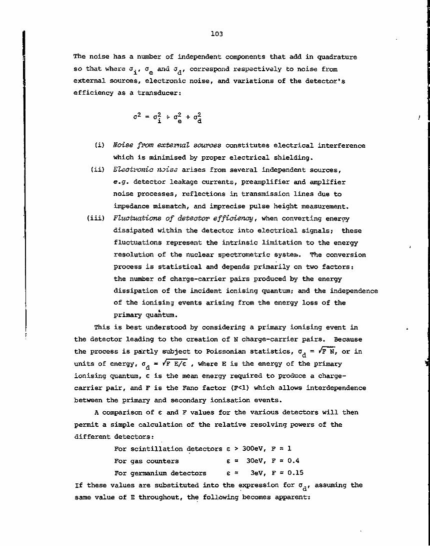
103
The noise has a number of independent components that add in quadrature
so that where a., a and a,, correspond respectively to noise from
external sources, electronic noise, and variations of the detector's
efficiency as a transducer:
o2 = a? fa 2* a2l e d
(i) Noise from external sources constitutes electrical interference
which is minimised by proper electrical shielding,
(ii) Electronic noise arises from several independent sources,
e.g. detector leakage currents, preamplifier and amplifier
noise processes, reflections in transmission lines due to
impedance mismatch, and imprecise pulse height measurement,
(iii) Fluctuations of detector efficiency, when converting eneroy
dissipated within the detector into electrical signals; these
fluctuations represent the intrinsic limitation to the energy
resolution of the nuclear spectrometric system. The conversion
process is statistical and depends primarily on two factors:
the number of charge-carrier pairs produced by the energy
dissipation of the incident ionising quantum; and the independence
of the ionising events arising from the energy loss of thet
primary quantum.
This is best understood by considering a primary ionising event in
the detector leading to the creation of N charge-carrier pairs. Because
the process is partly subject to Poissonian statistics, a, = /F N, or in
units of energy, a, = /F E/e , where E is the energy of the primary
ionising quantum, e is the mean energy required to produce a charge-
carrier pair, and F is the Fano factor (F<1) which allows interdependence
between the primary and secondary ionisation events.
A comparison of e and F values for the various detectors will then
permit a simple calculation of the relative resolving powers of the
different detectors:
For scintillation detectors e > 300eV, F * 1
For gas counters e - 30eV, F = 0.4
For germanium detectors e - 3eV, F - 0.15
If these values are substituted into the expression for a,, assuming the
same value of E throughout, the following becomes apparent:

104
(i) The resolving power of germanium detectors is intrinsically
at least 25 times better than that of scintillation detectors,
and approximately 5 times better than that of gas proportional
detectors.
(ii) The energy resolution of gas proportional detectors is better
than that of scintillation detectors by a factor of 5.
5. PROPORTIONAL COUNTERS
The detectors are of a cylindrical coaxial construction, similar to
Geiger-Mueller (GM) counters, and may employ the same filling gases,
e.g. argon or krypton with a small component of quenching gas (halogens
or organics), to suppress secondary photon emission. The gas that is
most commonly used for low energy photon and electron spectrometry is
P10, a mixture of 90 per cent argon and 10 per cent methane.
5.1 Operating Characteristics
Proportional counters have a counting rate/applied potential
plateau, like that of GM counters, with particularly small
slopes and extended operating ranges. The externally applied
potential is normally in the range 1000 to 2500 V. With3He detectors for neutron spectrometry, operation is sometimes
above 4500 V.
The gas multiplication factor varies from 1 to 10 000 with
increasing voltage in the proportional region, and decreases
with increasing gas pressure.
The range of gas filling pressures is usually between 7 and
25 cm Hg, but occasionally the detectors are filled to
operate with an internal pressure of about 1 atmosphere.
Reproducibility of operating characteristics is highly
dependent on the stability of voltage supplies and ambient
temperature.
Pulse duration times may be 'clipped1 to as little as 0.3
ys if high resolution spectrometry is not required. For
good resolution, a large proportion of the induced charge
from the transport of the positive ion sheath should be
collected in addition to the electron current. Most of the
charge is induced after a few microseconds, allowing effective
spectrometric operation with pulse clipping time constants of
between 3 and 5 microseconds.

105
Since the energy required per ion pair is about 30 eV in most
gases, a typical voltage output pulse, for a 6 keV electron
giving up its total energy in the cylinder, can be predicted
from the following formula:
V" = 0.5 MN
where N = number of ion pairs produced (200 in this example) ,
e = electronic charge of each ion (1.6 x 10 19 C) ,
M = gas multiplication factor (1000) , and
C = capacitance of the detector (20 pF) .
In this case V" = 1.6 mV.
The expected range of output signals will vary in practice from
0.2 to 20 mV, depending on the absorbed energy and on the multiplication
factor.
5.2 Application to Mineral Analysis
X-Ray spectrometry
The main advantages of proportional counters are that they give
reasonably good resolution and efficiency for photons with energies
below 20 keV, and they do not require cooling as do semiconductor detectors.
Their application to assaying problems is being supplanted by semiconductor
detectors .
Neutron detection and spectrometry
This is the principal field -of application of proportional counters
for borehole logging and bulk sample analysis.
BF- filled counters are sensitive to thermal neutrons only.
Their operation is based on the 10B (n,o) reaction. The boron used to
produce this gas is enriched boron, i.e. approximately 96 per cent B.
The reaction for thermal neutrons with a cross section of 3840 barns is•
n + 10B •*• 7Li + a + 2.31 MeV + y
where the emitted a-particle carries away about 1.5 MeV to produce
ionisation in the detector. The sensitivity of such counters is ~ 1 to
30 counts per second (cps) per unit thermal neutron flux. Standard
designs enable operation up to temperatures of 100°C, whereas special
processing allows an upper limit of 150°C.
Maximum filling pressures are 90 cm Hg for 2 in. diameter tubes,
and 140 cm Hg for 1 in. diameter tubes. Operation in yray fields is
possible below 100 rad h"1 (278 yGy s 1) , to avoid undue pulse pile-up
and gas deterioration.

106
zHe proportional counters operate on the basis of the following
(n,p) reaction:
I 3He + n •*• 3H + p + 765 keV
The cross section, starting from a value of 5400 barns for thermal
neutrons, falls off smoothly with a 1//E~ dependence without resonancesi n
j or excited daughter products. The reaction products therefore share the
initial neutron energy E plus 765 keV, and thus provide scope for use
! in fast neutron spectroscopy applications.
! Fast neutron spectroscopy is enabled by filling the detector to
high pressures and adding a minor but significant percentage of krypton
which has much greater stopping power than 3He and is far less costly,i -: A commonly used combination for gas filling is 3He at 6 atm and Kr at
'. 2 atm. They may also be operated at ambient temperatures up to 150°C.
' Special problems for spectroscopic applications
i (i) Incomplete absorption of the energy of the reaction productsi
if the interaction occurs near the counter wall. This
'wall-effect1 is particularly serious with 3He counters owing
' to the low stopping power of the gas. The problem i? reduced
! by increasing the stopping power by raising the 3He pressure1 and adding krypton. This reduces the proportion of events
; occurring too close to the wall.1 (ii) Elastic collisions of fast neutrons produce 3He recoils. The
cross section for elastic scattering is, in fact, about twice
that of the (n,p) reaction. This effect can produce a spectral
continuum which masks fast neutron spectral lines of lower
energy groups. The problem is minimised by using pulse rise
time discrimination,
(iii) These detectors have a much greater Y~raY sensitivity than
BF3 counters. It is so significant that the operation of 3He
detectors is limited to Y~*ay fields of less than
1 rad h'1 (2.78 yGy s"1). Pulse shape discrimination is
useful for rejecting large composite pulses resulting from the
pile-up of several y-ray pulses detected almost simultaneously.

107
Performance advantages
(i) The 3He detector is capable of good energy resolution
(5 per cent FWHM). In fact, this is an excellent quality
considering the general purpose operation and portability
of the detector.
(ii) Although the intrinsic efficiency for thermal neutrons is
appreciably higher than for BFa counters, it is most
important that the high filling gas pressure provide
relatively high efficiency for epithermal neutron
detection, e.g. a 3He detector operating at 10 atm has an
efficiency of about 30 per cent for 1 eV neutrons, 10 per
cent for 20 eV neutrons, and 3 per cent for 100 eV neutrons
(see figure 4). This factor is particularly important in both
bulk analysis and borehole logging applications. The epithermal
neutron measurement is a very reliable basis for porosity
<iaterminations.
100
u£
3He DETECTOR(1 in. DIAM)
1-0 10-0 100
NEUTRON ENERGY(eV)
1000
FIGURE 4
EFFICIENCY OF 3He DETECTOR
6. SOLID DEFECTORS FOR GAMMA-RAYS
Nal(Tl) scintillation detectors and germanium and silicon detectors
are widely used, as gas counters have severe limitations for y~ray
detection.
Proportional counters are fast but provide effective photon spectrometry
only to low energy X-rays; this is overcome by the use of the solid
detectors. Their basic characteristics for spectrometry are as follows:
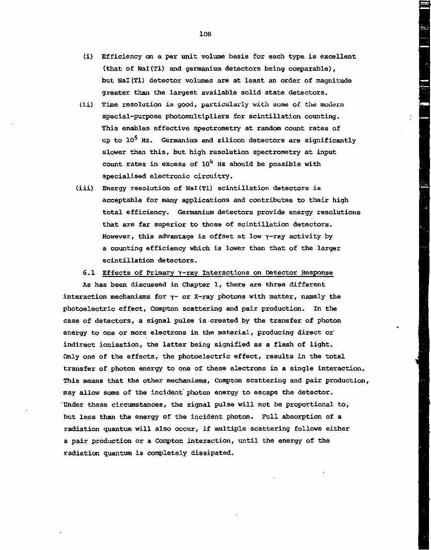
108
(i) Efficiency on a per unit volume basis for each type, is excellent
(that of Nal(Tl) and germanium detectors being comparable),
but Nal(Tl) detector volumes are at least an order of magnitude
greater than the largest available solid state detectors,
(ii) Time resolution is good, particularly with some of the modern
special-purpose photomultipliers for scintillation counting.
This enables effective spectrometry at random count rates of
up to 10 Hz. Germanium and silicon detectors are significantly
slower than this, but high resolution spectrometry at input
count rates in excess of 101* Hz should be possible with
specialised electronic circuitry,
(iii) Energy resolution of Nal(Tl) scintillation detectors is
acceptable for many applications and contributes to their high
total efficiency. Germanium detectors provide energy resolutions
that are far superior to those of scintillation detectors.
However, this advantage is offset at low y-ray activity by
a counting efficiency which is lower than that of the larger
scintillation detectors.
6.1 Effects of Primary y-ray Interactions on Detector Response
As has been discussed in Chapter 1, there are three different
interaction mechanisms for y- or X-ray photons with matter, namely the
photoelectric effect, Compton scattering and pair production. In the
case of detectors, a signal pulse is•created by the transfer of photon
energy to one or more electrons in the material, producing direct or'
indirect ionisation, the latter being signified as a flash of light.
Only one of the effects, the photoelectric effect, results in the total
transfer of photon energy to one of these electrons in a single interaction.
This means that the other mechanisms, Compton scattering and pair production,
may allow some of the incident' photon energy to escape the detector.
'Under these circumstances, the signal pulse will not be proportional to,
but less than the energy of the incident photon. Full absorption of a
radiation quantum will also occur, if multiple scattering follows either
a pair production or a Compton interaction, until the energy of the
radiation quantum is completely dissipated.

109
The relative abundance of the three interaction processes will
depend on the primary photon energy and the electronic characteristics
of the atoms in the detector. These relative abundances are best interpreted
in terms of the linear absorption coefficients for the photoelectric,
Compton, and pair production processes:
vvvThe relationships that the nuclear attenuation coefficients have with
energy of the photon radiation and with the atomic number of the detector
material are summarised below :
Energy Dependence-.
y ~ 1/E 3*5 up to 0.5 MeV and flattens out toP Y
1/E at high photon energies
Z Dependence:
y ~ An EPr
~Z5
pr
These relationships suggest that the detector's spectral response
and efficiency, termed the 'response function1, is highly dependent on
the geometrical factors of: (a) volume; and (b) surface to volume
ratio. The density and average atomic number of the detector matrix are
also most important.
PlKHOPMkfollb)I38M«V Bo K X-ray
OOKMeV
kfaltbl0662 MeV
F.W.HM.
0.1 O.Z
FIGURE 5
0.4 asE(McV)(b)
0.6 0.7
GAMMA SPECTRA OF 2uNa AND 137Cs MEASUREDWITH (a) AN Nal(Tl) AND (b) A Ge(Li) DETECTOR

110
The response function is characterised in terms of the ratio
between the full absorption peak and the first and second escape peaks
from pair production, and the ratio between the full absorption peak and
the remainder of the spectrum, including the Compton continuum.
The raain features of a gamma-ray spectrum (figure 5) are described
below:
(i) The full absorption peak is due to those incident photons
where complete photon-energy absorption takes place within
the detector volume. This may result from any of the three
interaction processes, provided that there are enough photon
scattering events,
(ii) The Cofnpton continuum results from the absorption within the
crystal of energy transferred to electrons from less scattering
events than are required to stop the incident photon. It is
worth noting that the Compton continuum recorded from a set
of monoenergetic j-xays stops short of merging with the
full absorption peak. The gap in the spectrum is relatively
large for X-rays, e.g. for a 50 keV x-ray, the highest energy
in the Compton spectral continuum is approximately 40 keV
lower than the peak. However, for a 0.5 MeV Y~ ay, the
corresponding point in the spectrum is approximately 0.17 MeV
below the full absorption peak, whereas with 10 MeV y~rays,
the highest energy of the Compton continuum is at approximately
9.75 MeV.
(iii) The single escape peak results from escape of one annihilation
photon from the crystal, whereas the double escape peak is
due to the escape of both annihilation quanta. Their respective
locations are always fixed 0.51 and 1.02 MeV below the full
absorption peak.
(iv) The full absorption peak to Compton continuum ratio decreases
with energy but increases greatly with volume. The reason
for this is that the volume increase also increases the number
of scattering mean free paths within the detector for any
incident photon. This increases the probability for complete
photon energy absorption.

111
(v) The ratio between the pair peaks and the full absorption peak
increases with energy (figure 6), and decreases with volume.
However, the ratio between the two pair peaks is, in most
cases, almost independent of the primary photon energy for a
particular detector. Whatever sensitivity there is depends on
the 'range1 of the primary photon relative to the dimensions
of the detector.
0-4
>-2uj o-3uCu.UJ
Si c:P<_itute
0 1
iTYPICAL LARGE VOLUME 'COAX. GE(Li) DETECTOR /DoubleEFFICIENCY RELATIVE / Escape
TO 3 x 3 in. /•*•NA| ITI) CRYSTAL /FULL ABSORPTION /
'/
' y
i /'1 /1 / Full Absorption
Vs
8 9 1 0
FIGURE 6
RELATIONSHIP OF DETECTOREFFICIENCY TO ENERGY
With germanium detectors, the response function above 4 MeV has
similar attributes for the ratio between the larger of the escape peaks
and the full absorption peak. However for lithium-drifted detectors,
much depends on the depth of drift, hence it is impossible to generalise
about the ratio between the two escape peaks.
For y-rays having energies greater than 2.5 MeV, at least one of
the two escape peak*; is larger than the full absorption peak. With
semiconductor detectors, and with scintillation detectors having crystal
sizes smaller than 76 x 76 mm, the single escape peak is generally
smaller than the double escape peak. For crystal sizes equivalent to 76
x 76 mm and larger, the ratio is reversed. However, the reversal of the
ratio is only apparent above 6 MeV for the very large detectors now
available.
X-ray speotrometrio detectors have a response that is derived
largely from photoelectric absorption; Compton scattering provides the
unwanted background. This is the case with any matrix, whether solid or
gaseous.

112
KaX-Roy52keV
Tm 170
K^X-Ray
57.5 keV Photopeak84 keV
Iodine EscapeX-Roy Peak24 keV
SO 100
PHOTON ENERGY
FIGURE 7
TYPICAL X-RAY SPECTRA RECORDEDWITH Nal(Tl) AND Ge(Li) DETECTORS
Typical X-ray spectra recorded with both Nal(Tl) and Ge(Li) detectors
are shown schematically in figure 7. In this spectrum, the Compton
continuum is less prominent than in the y-ray spectrum shown in figure 5.
The broad scintillation detector spectrum shows a satellite peak which
is quite prominent 28 keV below the main peak. This is due to the
escape of the 28 keV iodine X-ray. The narrower Ge(Li) spectrum also
shows a satellite escape peak, 10 keV below the energy of the main peak.
This corresponds to the escape of germanium X-rays but, because of its
relatively greater absorption, few escapes occur and a relatively
smaller satellite peak is the result with the Ge(Li) detector.
With gas filled detectors for j-rays, such as proportional counters,
the most important interactions are the photoelectric effect and pair
production, dependent on Z and Z2 respectively, where Z refers to the
atomic number of the wall material.
Conversely, no count is produced by secondary electrons if the
distance from their point of production to the central region of the
detector exceeds their range in the gas and residual wall material. In
detection, the Compton processes, which have production rates linearly
proportional to Z, are nevertheless relatively insensitive to the wall
material since electron range is also inversely proportional to the Z of
the material.

113
6.2 Efficiency of Solid State Detectors for Y-xay Detection
As previously mentioned, solid state detectors have a high efficiency
on a unit volume basis. In fact, Nal(Tl) and germanium detectors exhibit
very similar linear absorption characteristics over the greater part of
the energy range of y-rays used to analyse bulk mineral samples, i.e.
0.2 to 10 MeV, hence the two detectors also exhibit a fairly constant
ratio between their full absorption peak efficiencies (figure 6).
Efficiency characteristics of Nal(Tl) detectors are shown in figure 8
[Price 1965].1-0
o-s
UJCu. 0-2tu
8! 0-1
Ul(C. •05
•020-1 0-2 0-5 1-0 2-0 5-0 10-0
E (MEV)
FIGURE 8
EFFICIENCY CHARACTERISTICS OF Nal(Tl)DETECTORS
However, much larger volume crystals are fabricated in Nal(Tl) than
in germanium. For borehole logging, the size of the borehole is the
only constraint on the volume of the scintillators (i.e. ~ 500 cm3).
Fabrication of large volume germanium detectors is still a developing
technology, although detectors of approximately 100 cm3 are now possible.
This means that germanium detectors with efficiency in the range 15 to
25 per cent of 76 x 76 mm Nal(Tl) are becoming available.
The principal efficiency characteristics of interest to the user
are the full absorption peak efficiency and the escape peak efficiencies,
but not the total efficiency which includes the continuum response to
Compton scattering. As shown in figure 6, either of the escape peaks
may indeed become more prominent than the full absorption peak at high
photon energies.
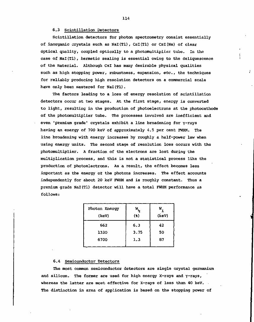
114
6.3 Scintillation Detectors
Scintillation detectors for photon spectrometry consist essentially
of inorganic crystals such as Nal(Tl), Csl(Tl) or Csl(Na) of clear
optical quality, coupled optically to a photomultiplier tube. In the
case of Nal(Tl), hermetic sealing is essential owing to the deliquescence
of the material. Although Csl has many desirable physical qualities
such as high stopping power, robustness, expansion, etc., the techniques
for reliably producing high resolution detectors on a commercial scale
have only been mastered for Nal(Tl).
The factors leading to a loss of energy resolution of scintillation
detectors occur at two stages. At the first stage, energy is converted
to light, resulting in the production of photoelectrons at the photocathode
of the photomultiplier tube. The processes involved are inefficient and
even 'premium grade1 crystals exhibit a line broadening for y-rays
having an energy of 700 keV of approximately 4.5 per cent FWHM. The
line broadening with energy increases by roughly a half-power law when
using energy units. The second stage of resolution loss occurs with the
photomultiplier. A fraction of the electrons are lost during the
multiplication process, and this is not a statistical process like the
production of photoelectrons. As a result, the effect becomes less
important as the energy ot the photons increases. The effect accounts
independently for about 20 keV FWHM and is roughly constant. Thus a
premium grade Nal(Tl) detector will have a total FWHM performance as
follows:
Photon Energy
(keV)
662
1330
6700
\(%)
6.3
3.75
1.3
Wi(keV)
42
50
87
6.4 Semiconductor Detectors
The most common semiconductor detectors are single crystal germanium
and silicon. The former are used for high energy X-rays and -rays,
whereas the latter are most effective for X-rays of less than 40 keV. .
The distinction in area of application is based on the stopping power of

115
silicon which is lower than that of germanium; hence a thin wafer of
silicon will have a particularly low efficiency for higher energy photons,
which reduces the Compton continuum background. Until recently, Si and
Ge detectors were fabricated by drifting Li ions through the matrix of
the semiconductor, thus creating a sensitive volume of high resistance.
This requires cooling to low temperatures (liquid nitrogen) , not only
for operation, but also for storage. A significant rise in temperature
causes precipitation of Li ions and detector failure.
With the production of ultra-pure germanium, drifting is no longer
necessary and, although super-cooled operation is still required, accidental
warm-up no longer spells disaster. This is certainly an important
consideration since, on the basis of equivalent detection efficiency,
germanium detectors are still more costly than Nal (Tl) detectors by more
than an order of magnitude.t
Intrinsic energy resolution, W. , for semiconductor detectors depends
on the total number of ion pairs produced, the Y-xay energy E, and the
energy of ion pair formation e. Thus W. = 2.36 (FE/e) . Here the
statistical Fano factor F is about 0.12 for both germanium and silicon,
and e at 90 K for these materials is about 3.0 and 3.8 eV respectively.i
The table below gives values for both the intrinsic resolution W.
and the actual resolution W. for Si and Ge detectors:
Photon Energy
6.4 keV
14.4 keV
1 MeV
4 MeV
10 MeV
W.[ (Ge)
1.4 keV
2.8 keV
4.4 keV
W^ (Si)
125 eV
195 eV
W± (Ge)
1.9 keV
W. (Si)
195 eV
270 eV
To obtain full advantage of these detectors, which have a resolution
FWHM between 0.1 and 1 per cent, great care is necessary to minimise
both electronic and pick-up interference noise.•
7. INSTRUMENTAL ENERGY CALIBRATION
In most situations, the energy calibration of instrumentation, in
terms of keV per unit of pulse height, is most conveniently made, using
y-ray reference sources, before the assaying measurement is carried out.

116
It is assumed that the measurement system has a virtually linear response
which will be preserved by gain and zero threshold stabilisation. This
approach gives only a first order of accuracy; whether a second stage of
calibration should be carried out with a computer is determined by the
particular assaying problem. The response of a spectrometer is rarely
perfectly linear, and interference with the gain stabilisation process
will occur from a sloping spectral continuum. Thus, if a slope under the
spectral peak is used for stabilisation, gain calibration errors and
gain variations will occur, unless compensation is made at the computational
stage.
Small computers which can be directly interfaced with the spectro-
metric system provide a much greater scope for interpretive processing
than hardwired systems. They can be utilised in a real-time or on-line
mode to record data while computing. It is more often convenient to
arrange a tandem operation, where the computer is dedicated to interpreting
the immediately preceding measurement while the spectrometric system
simultaneously records data into an independent memory bank from the
current measurement. At the end of spectral recording, a transfer is
made from the independent memory bank to that of the computer, and the
analysis process is recommenced for the next sample.
8. SPECTRAL PEAK ANALYSIS
8.1 Analysis of Peak Area
The information required about the mineral, or about any of its
components, is characterised most clearly by the areas of several of the
spectral peaks, the duration of the measurement, and other parameters.
For instance, one such parameter might be the response flux of thermal
neutrons that may have been measured either directly in a separate
measurement, or indirectly from the peak area of the 478 keV y-rays
emitted fron. a boron foil adjacent to the detector.
Although the spectral peak represents only a fraction of the total
spectral response from the sample, it provides the basis for the simplest
and most direct method of evaluating grade while measurement is in
progress. There are two common approaches:
(i) If there is a single peak, it can be assumed that its shape
follows the 'normal error' curve so that its area A is given
. by:
A » 1.06.h.w.
where h and w. are the height and half width of the peak above
the underlying spectral continuum. Since both of these
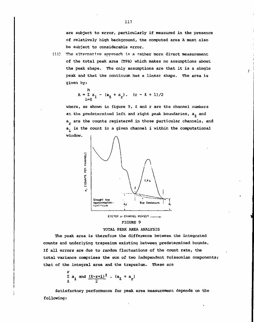
117
(ii)
are subject to error, particularly if measured in the presence
of relatively high background, the computed area A must also
be subject to considerable error.
The alternative approach is a rather more direct measurement
of the total peak area (TPA) which makes no assumptions about
the peak shape. The only assumptions are that it is a single
peak and that the continuum has a linear shape. The area is
given by:
ha. - (a + a ) .
* r(r - I + l)/2
where, as shown in figure 9, Si and r are the channel numbers
at the predetermined left and right peak boundaries, a. and
a are the counts registered in those particular channels, and
a. is the count in a given channel i within the computational
window.
0-
U1
Straight lineapproximation'ccni'^uum
, . ^=*-s;1 True Continuum !,*i
rir
i
Eti£?GY cr CHANNEL NUDES'? _
FIGURE 9
TOTAL PEAK AREA ANALYSIS
The peak area is therefore the difference between the integrated
counts and underlying trapezium existing between predetermined bounds.
If all errors are due to random fluctuations of the count rate, the
total variance comprises the sum of two independent Poissonian components;
that of the integral area and the trapezium. These are
rZ a. and (A-r+1)2 . (a, + a )% i 2 * r
Satisfactory performance for peak area measurement depends on the
following:
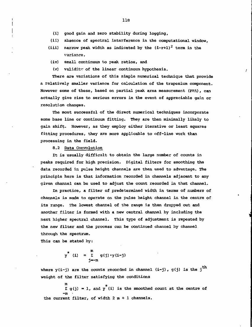
118
(i) good gain and zero stability during logging,
(ii) absence of spectral interference in the computational window,
(iii) narrow peak width as indicated by the U-r+1)2 term in the
variance,
(iv) small continuum to peak ratios, and
(v) validity of the linear continuum hypothesis.
There are variations of this simple numerical technique that provide
a relatively smaller variance for calculation of the trapezium component.
However some of these, based on partial peak area measurement (PPA), can
actually give rise to serious errors in the event of appreciable gain or
resolution changes.
The most successful of the direct numerical techniques incorporate
some base line or continuum fitting. They are then minimally likely to
gain shift. However, as they employ either iterative or least squares
fitting procedures, they are more applicable to off-line work than
processing in the field.
8.2 Data Convolution
It is usually difficult to obtain the large number of counts in
peaks required for high precision. Digital filters for smoothing the
data recorded in pulse height channels are then used to advantage. The
principle here is that information recorded in channels adjacent to any
given channel can be used to adjust the count recorded in that channel.
In practice, a filter of predetermined width in terms of numbers of
channels is made to operate on the pulse height channel in the centre of
its range. The lowest channel of the range is then dropped out and
another filter is formed with a new central channel by including the
next higher spectral channel. This type of adjustment is repeated by
the new filter and the process can be continued channel by channel
through the spectrum.
This can be stated by:
* m
y (i) = E g(j)-y(i-j)j=-m
where y(i-j) are the counts recorded in channel (i-j), g(j) is the j
weight of the filter satisfying the conditions
m *2 g(j) = I/ and y (i) is the smoothed count at the centre of
-m •the current filter, of width 2 m + 1 channels.
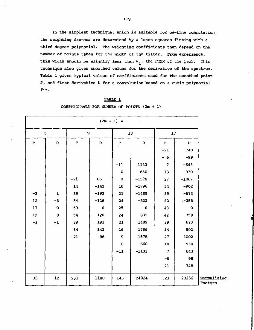
119
In the simplest technique, which is suitable for on-line computation,
the weighting factors are determined by a least squares fitting with a
third degree polynomial. The weighting coefficients then depend on the
number of points taken for the width of the filter. From experience,
this width should be slightly less than w. , the FWIIM of the peak. This
technique also gives smoothed values for the derivative of the spectrum.
Table 1 gives typical values of coefficients used for the smoothed point
F, and first derivative D for a convolution based on a cubic polynomial
fit.
TABLE 1
COEFFICIENTS FOR NUMBER OF POINTS (2m + 1)
(2m + 1) -
5
F
*»3
12
17
12
-3
35
D
1
-8
0
8
-1
12
9
F
-21
14
39
54
59
54
39
14
-21
231
D
86
-142
-193
-126
0
126
193
142
-86
1188
13
F
-11
0
9
16
21
24
25
24
21
16
9
0
-11
143
D
1133
-660
-1578
-1796
-1489
-832
0
832
1489
1796
1578
660
-1133
24024
17
F
-21
- 6
7
18
27
34
39
42
43
42
39
34
27
18
7
-6
-21
323
D
748
-98
-643
-930
-1002
-902
-673
.-358
0
358
673
902
1002
930
643
98
-748
23256 NormalisingFactors
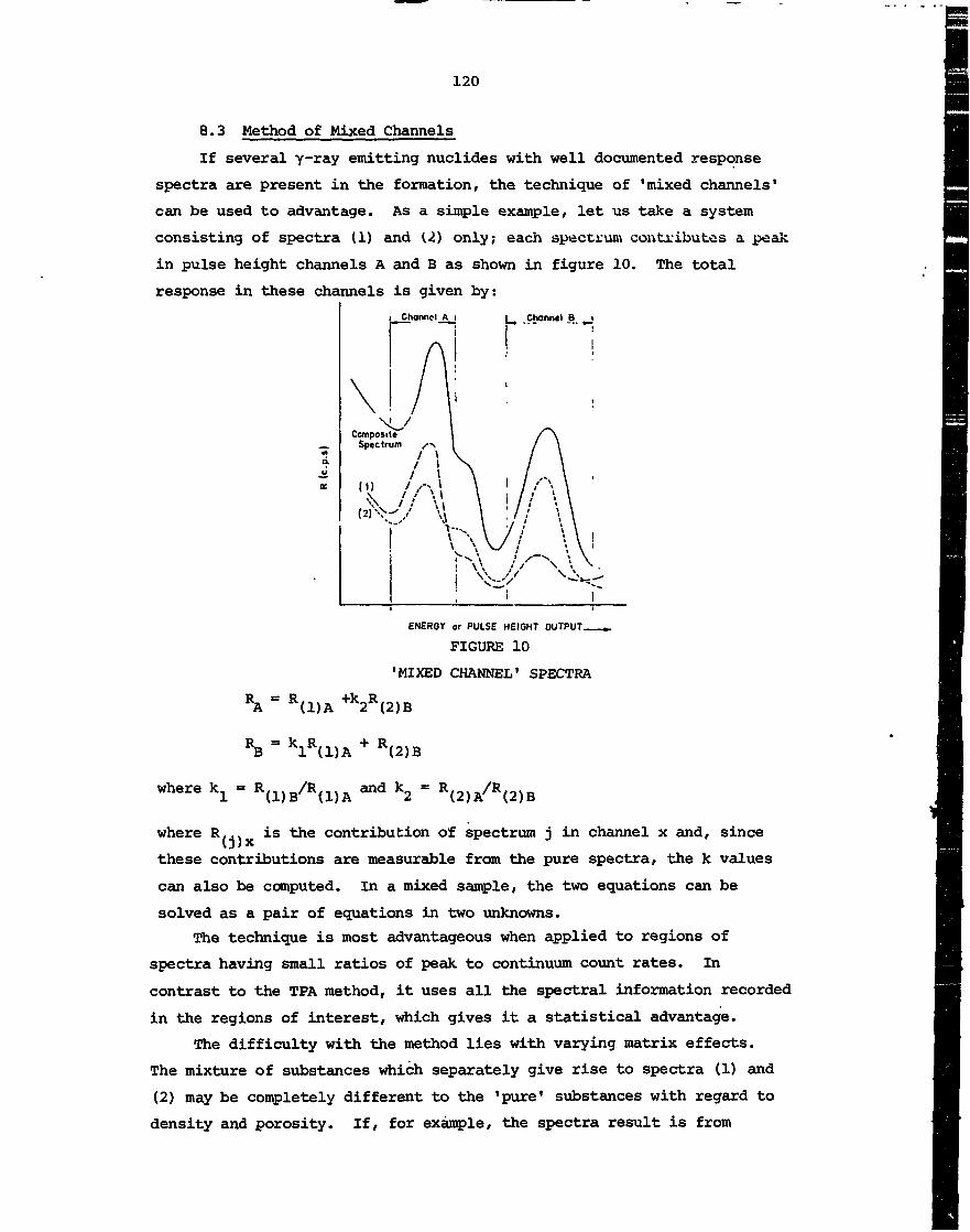
120
8.3 Method of Mixed Channels
If several j-xay emitting nuclides with well documented response
spectra are present in the formation, the technique of 'mixed channels'
can be used to advantage. As a simple example, let us take a system
consisting of spectra (1) and (2) only; each spectrum contributes a peak
in pulse height channels A and B as shown in figure 10. The total
response in these channels is given by:
_Choniwl_Aj Channel B_
ENERGY or PULSE HEIGHT OUTPUT
FIGURE 10
'MIXED CHANNEL1 SPECTRA
RA R(1)A +k2R(2)B
where k.
klR(l)A
R(1)B/RU)A
(2)B
R(2)A/R(2)B
where R... is the contribution of spectrum j in channel x and, sinceO *
these contributions are measurable from the pure spectra, the k values
can also be computed. In a mixed sample, the two equations can be
solved as a pair of equations in two unknowns.The technique is most advantageous when applied to regions of
spectra having small ratios of peak to continuum count rates. In
contrast to the TPA method, it uses all the spectral information recorded
in the regions of interest, which gives it a statistical advantage.
The difficulty with the method lies with varying matrix effects.
The mixture of substances which separately give rise to spectra (1) and
(2) may be completely different to the 'pure1 substances with regard to
density and porosity. If, for example, the spectra result is from
121
neutron activation, the relative heights of different spectral peaks
could be altered.
9. SUMMARY
There are more sophisticated and expensive methods of spectral
analysis than described here, but they are outside the scope of this
series of lectures. In conclusion, spectrometry and spectal analysis
are possible at many qualitative'and quantitative levels of precision.
However, the controller of grade or mineral quality must investigate the
level of interpretation most appropriate to the particular process under
consideration.
10. BIBLIOGRAPHY
Adams/ F. s Dams, R. [1970] - Applied Gamma-ray Spectrometry. Pergamon
Press, Oxford.
De Soete, D., Gijbels, G. & Hoste, J. [1972] - Neutron Activation. John
Wiley & Sons, London, pp.215-216.
England, J.B.A. [1974] Techniques in Nuclear Structure Physics. London.
Price, W.J. [1965] - Nuclear Radiation Detection. McGraw-Hill, New York,
p.190.
Savitzky, A. & Golay, M.J.E. [1964] - Smoothing and Differentation Data
By Simplified Least Squares Procedures. Anal. Chem., 36: 1627-1637.
123
CHAPTER 3
GAMMA-RAY AND NEUTRON SOURCES
R.J. HOLMES

125
1. GAMMA-RAY SOURCES
Most y-ray sources in commercial use do not occur in nature
because their half-lives are small compared with geological times. They
must be produced from naturally occurring nuclides by a suitable nucle?r
reaction; often this is by irradiation in a nuclear reactor.
Some examples of radioisotope production are given below:
59Co (n,y)60Co T^123Sb (n,y)mSb T^
6Li (n,a)3H T^55Mn (p,n)55Fe T,
5.26 y
60 d
12.3 y
2.7 y
Commercially available sources are sealed in chemically inert capsules.
The choice of the most suitable source for a particular application
usually depends on the energy of the y-rays that are emitted and on the
half-life of the radioisotope. In many applications, a monoenergetic
source of long half-life is preferred. Calibration corrections for
source decay can be made using the familiar equation
- 0.693t/T,= I eo
where I is the initial source intensity/ I(t) is its intensity at timeo
t, and T, is the half-life. Selection of the appropriate y-ray energy
depends on such criteria as the energy threshold for a desired nuclear
reaction and whether absorption should be due predominantly to the
photoelectric effect or Compton scattering. Table 1 lists the commonly
used y-ray sources together with their y-ray energies and half-lives.
2. X-RAY SOURCES
Sources of radiation below an energy of about 150 keV are usually
referred to as X-ray sources, although technically some of them are low
energy y-ray sources, e.g. 21flAm and 57Co, because the radiation orig-
inates from the nucleus. A number of different types are available:
(i) Isotopic primary X-ray sources (more correctly referred to as
low energy photon sources).
(ii) Isotopic secondary X-ray sources (gamma or beta excited).
(iii) X-ray tubes.
The primary X-ray sources are radioisotopes sealed in a capsule,
normally having a thin window to minimise absorption of the low energy
photons. The most commonly used sources of this kind are listed in
table 2.

126
TABLE 1
COMMONLY USED GAMMA-RAY SOURCES
Isotope
Caesium-137
Barium-133
Cobalt-60
Sodium-22
Manganese-54
Zinc-65
Selenium-75
Yttrium-88
Iridium-192
Antimony-124
Mercury-203
Symbol
137CS
133Ba
6°Co22Na5l*Mn
"zn
75Se
8 8Y192lr12l*Sb203Hg
Half-life
30.0 y
10.4 y
5.26 y
2.60 y
312 d
244 d
120 d
107 d
74 d
60 d
46 d
Main Y~r&y Energies(MeV)
0.662
0.384, 0.356, 0.303, 0.276, 0.081
1.332, 1.173
1.275, 0.511
0.835
1.116
0.401, 0.280, 0.265, 0.136
1.836, 0.898
0.468, 0.316, 0.308, 0.296
2.091, 1.691, 0.723, 0.603, 0.121
0.279
TABLE 2
PRIMARY LOW ENERGY PHOTON SOURCES
Isotope
Americium-241
Plutonium-238
Lead-210
Curium-244
Iron-55
Europium-155 '
Cadmium-109
Samarium-145
Cobalt-57
Gadolinium-153
Iodine -125
Symbol
2t»1Am
238pu210pb
2tfl+Cm55Fe
155EU
109Cd '1It5Sm57Co153Gd
125l
Half-life
458 y
86 y
20.4 y
17.9 y
2.6 y
1.8 y
453 d
340 d
270 d
242 d
60 d
Main Photon Energies(keV)
60
13-21
47
14-21
5.7
105, 87, 43-49
88, 22-25
61, 38-44
122, 136
103, 98, 41-48
35, 27-31
Secondary X-ray sources rely on isotopic 0- or y*ay excitation of
a target for production of the X-rays. Examples of beta excited or
'bremsstrahlung1 sources are 3H/Ti and llf7Pm/Zr-Al which produce X-rays
of 2-10 keV and 10-60 keV, respectively. These sources are an intimate

127
mixture of -emitting radioisotopes and a target material. The X-rays
result from deceleration of the electrons from the beta source as they
strike the target material. The energy distribution of the bremsstrahlung
X-rays depends on the energy of the 3-particles (i.e. electrons). Char-
acteristic X-rays from the target atoms are also produced because of the
K or L shell ionisation. A spectrum of the excited X-rays from a llf7Pm/Zr-
Al source is shown in figure 1.
$(U
z
>
100ZrKaX-roys
X-roys
FluorescentX-roy
10 20 30 40ENERGY (keV)
FIGURE 1
SPECTRUM OF EXCITED X-RAYS FROM Alk7Pm/Zr-Al BREMSSTRAHLUNG SOURCE
Tungsten alloyshield
Target material
Rodiois iourc*
FIGURE 2
PRINCIPLE OF Y-RAY EXCITEDX-RAY SOURCES
The principle of gamma-excited X-ray sources is illustrated in
figure 2. A target material is irradiated by a radioisotope source such
as 2ltlAm, which excites the characteristic X-rays from the target. By
selecting various targets, e.gr. Cu, Mo and Ag, X-rays of different
energies can be obtained as shown in figure 3.
100
uzUJs
Ci
•
j Rb
('At
r.
I
j &
L
a T
i
' - — Target
— K«X- rays
|"*~X-roys
A ,10 20 30 40 50 60
ENERGY (keV)
FIGURE 3
SPECTRA OF Y-RAY EXCITED X-RAYS FORVARIOUS TARGET MATERIALS
The Ka X-ray peak heights have beennormalised to the same relative intensity

128
In the case of X-ray tubes, an example of which is shown in figure
4, electrons from a heated filament are accelerated towards the anode by
a potential of several tens of ki3.ovolts. Upon striking the target
material embedded in the anode, bremsstrahlung X-rays are produced. An
example of a spectrum from an X-ray tube is shown in figure 5. The
maximum energy of the X-rays is V keV, where V is the accelerating
voltage in kilovolts; characteristic X-rays are also produced from the
target.
High-voltage source
FIGURE 4
SCHEMATIC OP AN X-RAY TUBE
ENERGY
FIGURE 5
TYPICAL SPECTRUM OF X-RAYS FROM ANX-RAY TUBE
Isotopic X-ray sources and tubes have several advantages and dis-
advantages. The isotopic sources are more compact than X-ray tubes, and
require no electronic equipment or high voltage power supplies for the
production of X-rays. The X-ray output from isotopic sources is also
very stable, and needs only to be corrected for source decay. On the
other hand, X-ray tubes can be turned off if necessary, and offer greater
X-ray output intensity than isotopic sources. There is also greater
scope for the variation of X-ray energy.
3. NEUTRON SOURCES
Neutron sources fall into two main categories. The first category
is isotopic and includes (a,n) , fission and photoneutron sources; the
second covers neutron generators.
3.1 (g,n) Sources
When an a -emitting nuclide is mixed with a light element, usually
beryllium, neutrons are produced by the following reaction:
Be 12 n
Neutron outputs in excess of 107 neutrons per second (n s"1) are readily

129
obtained. Because the 12C nucleus is left in an excited state, some
4.43 MeV y-radiation is also emitted. The a-emitter and the beryllium
are usually in powder form. Consequently, because considerable care
must be taken to avoid leakage, the source material is doubly sealed in
stainless-steel capsules. An exception is plutonium (238Pu or 239Pu),
which can be alloyed with beryllium to produce a solid (ct,n) Pu-Be
source. As a precaution, however, the alloy is still encapsulated in
stainless steel. The dimensions of the encapsulated sources depend on
the neutron output. For example, 10 Ci (370 GBq) 2tflAm-Be sources
emitting about 2 x 10⁷ n s~* are sealed in cylindrical capsules of 30 mm
diameter and 60 mm length.
TABLE 3
(a,n) NEUTRON SOURCES
Source
2l°Po-Be242Cm-Be228Th-Be
2l Cm-Be227Ac-Be
238pu_Be
21tlAm-Be226Ra-Be
239pu_Be
2lflAm-B2^Am-F241Am-Li
Half-life
138 d
163 d
1.9 y
17.9 y
21.8 y
86.4 y
458 y
1 600 y
24 400 y
458 y
458 y
458 y
Neutron Emission(n s'1 Ci"1)*
2.5 x 106
2.5 x 10⁶
2.0 x 10⁷
2.5 x 10⁶
2.0 x 10⁷
2.2 x 10⁶
2.2 x 10⁶
1.3 x 10⁷
1.5 x 10⁶
5.0 x 10⁵
1.5 x 10⁵
4.0 x 101*
AverageNeutronEnergy(MeV)
4.3
4
-
4
-4
4
3.6
4.5
3
1.5
0.4
Gamma ExposureRate (mrad h"1)* at1 m per 106 n
<0.1
<1
30
<1
8
<1
1
60
<1
1
1
1
* 1 Ci =37 GBq 1 rad h"1 » 2.78 yGy s"1
Table 3 lists the properties of a number of (ct,n) sources; of these21flAm-Be is the most readily available. As indicated in table 3, other
target materials such as lithium/ boron, carbon, fluorine or oxygen-18
can be used. However, the neutron yield is much less than for beryllium.
The average neutron energy of the more widely used beryllium-based
sources is between 3.5 and 5 MeV, depending on the a-emitter used.
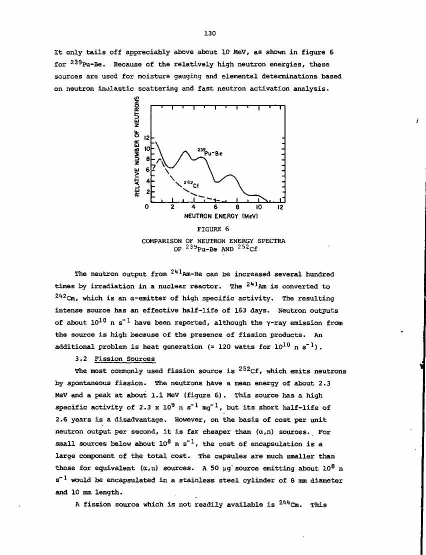
130
It only tails off appreciably above about 10 MeV, as shown in figure 6
for 239Pu-Be. Because of the relatively high neutron energies, these
sources are used for moisture gauging and elemental determinations based
on neutron inelastic scattering and fast neutron activation analysis.
uiec
12
108
6
4
2
239.PirBe
0 2 4 6 8 10 12NEUTRON ENERGY (MeV)
FIGURE 6
COMPARISON OF NEUTRON ENERGY SPECTRAOF 23yPu-Be AND 252Cf
The neutron output from 2tflAm-Be can be increased several hundred
times by irradiation in a nuclear reactor. The 21flAm is converted to2/t2Cm, which is an a-emitter of high specific activity. The resulting
intense source has an effective half-life of 163 days. Neutron outputs
of about 1010 n s"1 have been reported, although the y-xay emission from
the source is high because of the presence of fission products. An
additional problem is heat generation (= 120 watts for 1010 n s~M.
3.2 Fission Sources
The most commonly used fission source is 252Cf, which emits neutrons
by spontaneous fission. The neutrons have a mean energy of about 2.3
MeV and a peak at about 1.1 MeV (figure 6). This source has a high
specific activity of 2.3 x 10⁹ n s"1 mg"1, but its short half-life of
2.6 years is a disadvantage. However, on the basis of cost per unit
neutron output per second, it is far cheaper than (ct,n) sources. For
small sources below about 108 n s"1, the cost of encapsulation is a
large component of the total cost. The capsules are much smaller than
those for equivalent (o,n) sources. A 50 ng' source emitting about 108 n
s"1 would be encapsulated in a stainless steel cylinder of 8 mm diameter
and 10 mm length.
A fission source which is not readily available is 2lflfCin. This

131
has a lower specific activity (9 x 10³ n s""1 mg"1) than 252Cf but a
longer half-life (17.9 years).
Californium sources are used when fast neutrons are either not
required or undesirable. With good thermalisation, 2b2Cf is suitable
for thermal neutron capture or thermal neutron activation analysis
because interferences from fast neutron reactions with thresholds above
4-5 MeV are largely eliminated.
3.3 Photoneutron Sources
In contrast to isotopic (ct/n) sources, which emit a spectrum of
neutron energies, photoneutron or (y»n) sources emit near monoenergetic
neutrons when the yemitter is also monoenergetic. Since the photon
energy of isotopic y-xay sources rarely exceeds 3 MeV, only the (y,n)
reactions in beryllium (1.665 MeV threshold) and deuterium (2.225 MeV
threshold; need be considered. The following reaction occurs when
beryllium is irradiated with high energy y
3Be 8Be n
There are only a few Y~raY sources with acceptably long half-lives
that emit Y~rays above these thresholds. These are 12l*Sb (60 day half-
life) , 88Y (107 day half-life) and 226Ra (1600 year half-life) in equili-
brium with its daughters. The energy of the Y~radiation from 124Sb and88Y (see table 1) is sufficient to generate photoneutrons from beryllium
only. The radium source will generate photoneutrons from deuterium as
well. Although the long half-life of 226Ra is attractive, it is very
expensive; consequently, in most applications, photoneutron sources
based on 124Sb or 88Y are used. The characteristics of these two sources
are given in table 4. The high Y~raY dose rate at 1 metre should be
noted.
TABLE 4
COMMON PHOTONEUTRON SOURCES
Y-emitter
12"sb
88y
Half-life
60 d
107 d
Y-rayEnergies(MeV)
2.091
1.691
1.836
Target
Be
Be
AverageNeutronEnergy(keV)
26
200
NeutronYield
(n s'1 Ci'1)
-5 x 10⁶
3 x 10⁶
Gamma Dose-rate at 1 m
(mrad h'1 Ci"1)
-1000
-1000

132
Figure 7 shows a cross section through a typical 12tfSb-Be neutron
source. The inner antimony cylinder can be taken out of the beryllium
cylinder. Thus it is possible to turn the neutron source off at will,
although the y-radiation remains. The dimensions of the source capsule
depend on the size of the beryllium block. The Radiochemical Centre
(Amersham, UK) markets a 1 Ci 121*Sb-Be neutron source emitting 5.2 x 10⁶
n s,-1 The capsule is about 60 mm diameter and 80 mm long, which is
considerably larger than a comparable (oc,n) source.
Wire to supportsource
source
Berylliumcylinder
FIGURE 7
SCHEMATIC OF A 12l)Sb-Be NEUTRON SOURCE
The most important feature of photoneutron sources is that the
average neutron energy is in the keV region. This eliminates possible
interferences from fast neutron reactions. Photoneutron sources are
therefore best suited to thermal neutron activation analysis, although
their short half-lives and large -f-ray background are serious disad-
vantages. For this reason 2S2Cf is often used instead.
3.4 Neutron Generators
Many types of accelerators have been used to produce neutrons, but
commercially available units usually use one of the following reactions:
H
H
H
H
He
n
(D-D reaction)
(D-T reaction)
Typical neutron generators based on these reactions consist of an ion
source which produces ionised deuterium (2H) gas and a target containing
either deuterium or tritium (3H). The deuterons are accelerated up to
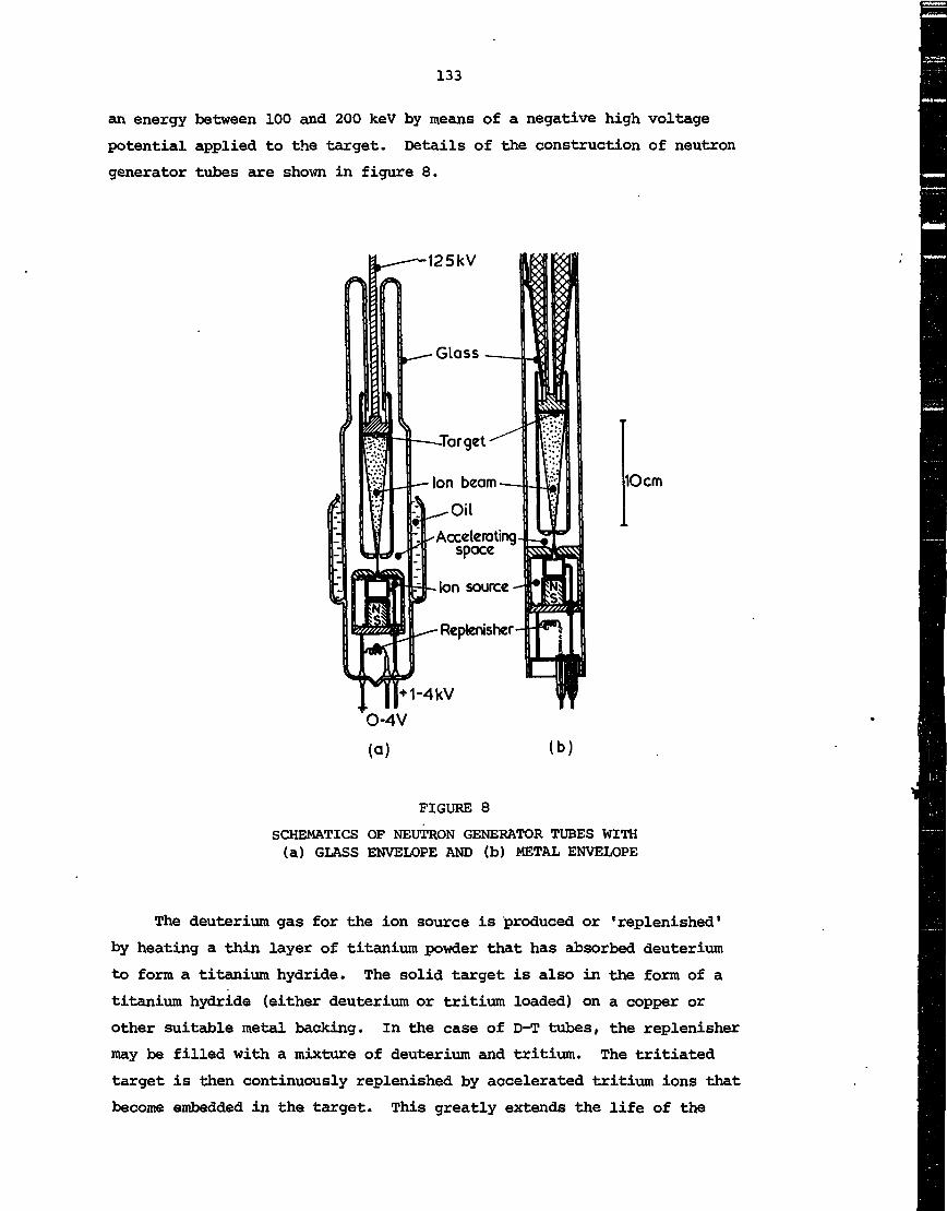
133
an energy between 100 and 200 keV by means of a negative high voltage
potential applied to the target. Details of the construction of neutron
generator tubes are shown in figure 8.
125kV
Gloss
Target""
Ion beam-
OilAccelerating
space
Ion source
Replenisher-
1Ocm
FIGURE 8
SCHEMATICS OF NEUTRON GENERATOR TUBES WITH(a) GLASS ENVELOPE AND (b) METAL ENVELOPE
The deuterium gas for the ion source is produced or 'replenished*
by heating a thin layer of titanium powder that has absorbed deuterium
to form a titanium hydride. The solid target is also in the form of a
titanium hydride (either deuterium or tritium loaded) on a copper or
other suitable metal backing. In the case of D-T tubes, the replenisher
may be filled with a mixture of deuterium and tritium. The tritiated
target is then continuously replenished by accelerated tritium ions that
become embedded in the target. This greatly extends the life of the
134
tube. In D-D tubes, the target is replenished by deuterium ions that
are not involved in the reaction. Neutron generator tubes with completely
'self-loading targets' can also be constructed using this technique.
The energy of the neutrons produced by the D-D and D-T reactions
are 2.6 and 14 MeV respectively. Because the yield is much higher in
the latter case (more than 100 times greater), the D-T tube is more
commonly used. Neutron outputs in excess of 108 n s""1 are readily
achieved, and some manufacturers claim tube lifetimes of over 2000
hours.
The advantages of neutron generators are that they give an intense
monoenergetic neutron flux and can be pulsed if necessary. The latter
feature adds considerably to their flexibility. They can also be switched
off when not in use. The high neutron energy from D-T tubes (14 MeV) is
particularly useful in applications involving neutron inelastic scatter-
ing and fast neutron activation analysis, when the reaction threshold is
above the range covered by (a,n) sources. The principal disadvantages
of neutron generators are that complex electronics are required for
their operation and the neutron output is not as stable as that from
isotopic sources. The limited tube life and its replacement cost are
also disadvantages in some applications.
4. SAFETY OF RADIOISOTOPE SOURCES
The encapsulation of radiation sources must provide the highest
possible source integrity together with minimum attenuation of the
required radiation by the encapsulation materials. If a compromise must
be made, e.g. for low energy photon sources, safety must always be the
prime consideration.
The quality control of radioactive sources can be divided into two
types of inspection:
(i) Routine checks during production.
(ii) Special tests on prototype capsules.
The routine checks include source dimensions, activity content and tests
for leakage and contamination. Stringent tests for leakage are an
essential feature of radioactive source production. The tests to which
prototype source capsules are subjected are listed in table 5. Each
test can be applied in several degrees of severity denoted in the table
as Classes 1 to 6. Results are expressed as a five digit ISO (Inter-
national Standard Organization) code to indicate the severity of the
tests; this code is prefixed by the letter C or E to show whether the

135
source activity is less or greater than certain limits. These limits
depend upon the toxicity, solubility and reactivity of the active com-
ponent of the source. Fox example, the ISO classification of 252Cf
neutron sources supplied by the Radiochemical Centre is C64544.
TABLE 5
CLASSIFICATION OF SEALED SOURCE PERFORMANCE STANDARDS
Test
Temperature
Externalpressure
Impact
Vibrations
Puncture
(ClassMNo test
No test
No test
No test
No test
|2 |-40"C(20min)+80'C(1h)
25kPa absolute toatmospheric pressure
50g from 1 m
30min25Hztp500Hzat50n peak amplitude
1 g from 1 m
3
-40*C(20min)+180"C(1h)
25kPa absolute to2 MPa absolute
200g from 1 m
30min25Hz to 50Hz at 5pnpeak amplitude andSOHzto90Hzat0-635mm amplitudepeak to peak and90Hzto500HzatlOjfr.lOgfromlm
4
-40-C(20min)+400'C(1h)and thermal shock400"C to 20"C
25kPa absolute to7MPa absolute
2kg from 1 m
90mm25Hzto80Hzat1 -5mm amplitudepeak to peak and80Hz to 2000HZat200n
50g from 1 m
|5-40*C(20min)+600-C(1h)and thermal shock60CTCto20*C
25kPa absolute to70MPa absolute
5kg from 1 m
300gfrom1m
|6
-40"C(20min)+800'C(1h)and thermal shock800 C to 20'C
25kPa absolute to170Mpa absolute20kg from 1m
1kg from 1m
Typical applications for which sealed radioactive sources may be
used, with minimum performance requirements as specified in ISO 2919,
are given in table 6. Often source designs exceed these recommendations.
TABLE 6
SEALED SOURCE PERFORMANCE REQUIREMENTS FOR TYPICAL APPLICATIONS
Sealed source use
Industrial radiography Unprotected sourceSource in device
Gamma gauges (medium and high energy) Unprotected sourceSource in device
Beta gauges and sources for low energy gamma gaugesor X-ray fluorescence analysis (excluding gas-filled sources)
Oil well loggingPortable moisture and density gauges (including hand heldor dolly transported)
General neutron source application (excluding reactor start-up)
Calibration sources, activity greater than 30uCi
Gamma irradiation sources Unprotected sourceSource in device
Ion generators Chromatography(source-device combination may be tested) Static eliminators
Smoke detectors
(Sealed source test and class 1| Temperature (Pressure (Impact (Vibration (Puncture |
44443
5
4
4
2
44
323
33333
6
3
3
2
33222
53322
5
3
3
2
43222
11
332
2
3
2
1
22122
53322
2
3
3
2
43122

136
5. BIBLIOGRAPHY
Beckurts, K.H. & Wirtz, K. [1964] - Neutron Physics, Springer-Verlag,
Berlin.
Erdtmann/ G. & Soyka, W. [1974] - The Gamma-ray Lines of the Radio-
nuclides. JtIl-1003-AC (Table 1) .
The Radiochemical Centre [Undated] - Radiation Sources for Laboratory
and Industrial Use. The Radiochemical Centre, Amersham, UK.
Watt, J.S. [1973] - Radioisotope On-Stream Analysis - Development
History of an Award-winning System. At. Energy Aust., 16 (4)
3-19.

137
CHAPTER 4
NUCLEONIC GAUGES
B.D. Sowerby

139
1. INTRODUCTION
The main interactions of nuclear radiation with matter are absorption,
scattering and excitation. These interactions are the basis of the
various types of nuclear gauges. These gauges utilise various types of
radiation, e.y. a-particles, 6-particles, neutrons and/or y-quanta.
Even though they are all based on nuclear radiation, there are significant
differences between che gauges that use charged particles ^a- and p-
particles) and those that use neutrons and y-quanta. Since the charged
particles interact strongly with matter through ionisation, their range
is very limited and consequently they can only supply information on the
properties of thin layers of matter. However, neutrons and Y-quanta
have much longer ranges and can therefore yield information on the
properties of much larger volumes of matter. A summary of nuclear
gauges for level thickness, density and moisture is given in table 1.
Material tobe measured
Radioactivesource
FIGURE 1
GENERAL SKETCH SHOWING A NUCLEARTRANSMISSION GAUGE IN A CONTROL LOOP
Figure 1 shows the general layout of an automatic system based on
the application of a nuclear gauge. Radiation emitted by the source is
attenuated by the material. The fraction of radiation reaching the
detector is converted into signals that are amplified and used to
control the process in such a way that the atteriuation of radiation by
material remains constant. In simpler cases, e.g. for individual thickness
or level gauges, there is no control and the output of the amplifier is
used to display the desired information concerning the material. A
gauge in which the source and detector are placed on opposite sides of
the material being measured is known as a transmission gauge. In some
cases, thickness and density may be measured with the source and detector

140
TABLE 1
TECHNIQUES EMPLOYED IN SOME NUCLEAR GAUGES FOR THEMEASUREMENT OF LEVEL, THICKNESS, DENSITY AND MOISTURE
PropertyMeasured Teclmique Typical Applications
Level
Thickness,or massper unit•
Coatingthickness
Density
Bulkdensity
Moisture
3-transmissiony-transmission
y-backscat ter
neutron- backscatterand transmission
a-transmission
B-transmission
Transmission of low-energy X-rays andbremsstrahlung
Transmission of high-energy y-radiation
fj -backscattery-backscatter
g-transmission(differentialmethod)
3-backscatter
X-ray fluorescence
a-transmission-transmission
y-transmission
y-transmissiony-backscatter
Slowing down offast neutrons
Liquids (not in widespread use).Liquids, powders, slurries, ores incontainers.
Liquids in tanks (not in widespread use)
Hydrogenous solids (e.g. coal) andliquids.
Very light-weight materials, e.g.cigarette paper.Light-weight materials, e.g.paper, plastic, metalsSheet metals.
Trimming hot-steel blooms;hot rolling;materials on conveyor belts.
Paper.Walls of pipes, tanks, process vessels.
Coated textiles and papers, e.g. leather-cloth, abrasive papers and cloths.
Zn on steel; Ba2SOif coating on photo-graphic paper.
Sn and Zn on Fe; precious metals on Cu.
Gases.Cigarettes; fluids and slurries in pipesand tanks; gases and gas-fluidisedsolids; gas-liquid emulsions; steam-waterratios, etc.
Fluids and slurries in pipes and tanks.
Soil; borehole cores.Soil measurements on the surface and inboreholes; rocks and ore measurements inboreholes.
Soil; rocks and ores; agriculturalproducts.

141
on the same side of the material. An instrument based on this principle is
known as a backscatter gauge.
A radioisotopic instrument is used to measure some quality X of a
material in terras of the output I of a radiation detector. The J-ri(*f.mffn<?nt-
sensitivityj S, is defined as the ratio of the fractional change 6l/I
in detector output which results from a given fractional change 6X/X in
the quality being measured, i.e.
_ _ 61 . fixS ~ ~I 7 X (1)
If the only source of error in a measurement is the statistical
variation in the number of recorded events, the coefficient of variation
in the value of the quality measured is:
6JCX
(2)
where n is the count rate and t the measurement time. To reduce this to
as small a value as possible, S, n or t, or all three of these variables,
should be increased to as high a value as possible. In many cases,
however, the time available for measurement is short. This is particularly
true of high-speed production lines of sheet material where only a few
milliseconds may be available for the measurement.
The precision or reproducibility of a measurement is defined in
terms of the ability to repeat measurements of the same quantity.
Precision is expressed quantitatively in terms of the standard deviation
from the average value obtained by repeated measurements. In practice,
it is determined by statistical variations in the rate of emission of
radiation, instrumental instabilities and variations in measuring con-
ditions.
The accuracy of a measurement is an expression of the degree of
correctness with which an actual measurement yields the true value of
the quantity being measured. It is expressed quantitatively in terms of
the deviation from the true value of the mean of repeated measurements.
The accuracy of a measurement depends on the precision and also the
accuracy of calibration. If the calibration is exact, then in the
limit, accuracy and precision are equal. When measuring a quantity such
as thickness, it is relatively easy to obtain a good calibration. When
analysing many types of samples, on the other hand, the true value is
often difficult to obtain by conventional methods and care may have to
be taken in quoting the results.
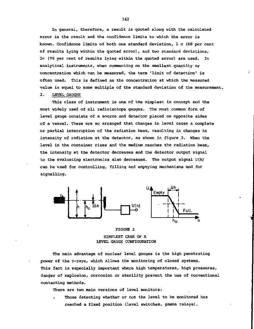
142
In general, therefore, a result is quoted along with the calculated
error in the result and the confidence limits to which the error is
known. Confidence limits of both one standard deviation, 1 a (68 per cent
of results lying within the quoted error), and two standard deviations,
2a (95 per cent of results lying within the quoted error) are used. In
analytical instruments, when commenting on the smallest quantity or
concentration which can be measured, the term 'limit of detection' is
often used. This is defined as the concentration at which the measured
value is equal to some multiple of the standard deviation of the measurement.
2. LEVEL GAUGES
This class of instrument is one of the simplest in concept and the
most widely used of all radioisotope gauges. The most common form of
level gauge consists of a source and detector placed on opposite sides
of a vessel. These are so arranged that changes in level cause a complete
or partial interruption of the radiation beam, resulting in changes in
intensity of radiation at the detector, as shown in figure .2. When the
level in the container rises and the medium reaches the radiation beam,
the intensity, at the detector decreases and the detector output signal
to the evaluating electronics also decreases. The output signal U(h)
can be used for controlling, filling and emptying mechanisms and for
signalling.
J k
h~^h 1 ,I—~l U hHF°FIGURE 2
SIMPLEST CASE OF ALEVEL GAUGE CONFIGURATION
The main advantage of nuclear level gauges is the high penetrating
power of the y-rays, which allows the monitoring of closed systems.
This fact is especially important where high temperatures, high pressures,
danger of explosion, corrosion or sterility prevent the use of conventional
contacting methods.
There are two main versions of level monitors:
Those detecting whether or not the level to be monitored has
reached a fixed position (level switches, gamma relays).

143
Those locating the level within a certain range (continuous
level monitor).
3. THICKNESS AND DENSITY GAUGES
The most commonly used gauges depend on the absorption of $-
particles or y-rays, and the source and detector are placed on opposite
sides of the sample. The detected intensity depends on the weight per
unit area of the sample. Thus for constant density, thickness changes
are measured, and for constant thickness, e.g. fluids in pipes, density
is measured.
If an absorber of mass per unit area m is placed between a radioactive
source emitting 8-particles or monoenergetic y-rays and a radiation
detector, the detector output (I) with absorber (I ) can be expressed by
the equation:
1 = 1 exp (- y.m) (3)
where y is the mass attenuation coefficient. This equation holds strictly
for collimated beam conditions, but only approximately for the broad
beam conditions found in practice.
Small changes in mass per unit area (6m) result in a change in
intensity (61):
— = - y.6m (4)
From equations (1) and (4), the instrument sensitivity is
S = y.m (5)
For high sensitivity, y should be made large by choice of the type and
energy of the radiation. However, sufficient radiation must be transmitted
so that the intensity can be accurately determined, and so that y is
not made too large. In practice, most gauges operate in the region 0.3
<y.m <3.
3.1 Thickness Gauges
Thickness gauges are commonly used for sheet materials such as
paper, plastics and metals; since these are usually between 1 and
1000 mg cm 2, beta sources are used. The accuracy of determination is
generally better than 1 per cent except for very light materials (<5 mg
cm 2) when it is about 2 per cent. For thicker materials, such as many
sheet metals, low energy y-ray sources are used.
Backscatter thickness gauges are used to advantage in the following
cases:
(i) When thin coatings are to be measured on thick base materials
(if the atomic numbers of coating ana base differ sufficiently).
The base must be of saturation thickness.

144
(ii) When there is not enough space for mounting a transmission
type detector, or where access is available to one side of the
material only.
However, measurement with backscatter gauges depends on the chemical
composition of the material to be gauged. This is generally a clear
disadvantage, since it limits the measuring accuracy for various material
compositions. For the measurement of plastic on steel, an application
often met with in industrial processes, approximately the same accuracies
(1-2 per cent) are achieved with backscatter gauges as with transmission
gauges. The useful ranges lie in the region of 30 per cent of the
transmission gauge ranges.
3.2 Density Gauges
Unlike thickness gauges, where the density of the measured sheet is
usually constant, the path length of the radiation beam in the material
is constant for density gauge applications. Therefore the correlation
between the signal output of the detector and the physically relevant
weight per unit area gives the correlation between the density of the
material measured and this output signal as well. Except for a very few
applications (e.g. the density of cigarettes, where B-radiation is used),
only y-rays, usually from 137Cs or 2ltlAm, are \ised for density gauging.
Since, in general, density ranges are centred around a fixed density
value, the range band is much lower than that of the thickness band with
thickness gauges. This means that in many cases the absorption law
given in equation (3) can be approximated by a straight line; this
decreases to a large extent the difficulties of signal processing. For
constant chemical composition the accuracy of measurement is often ±0.1
per cent relative.
The density can often be used as an indicator for other physical or
chemical properties of a substance, such as concentrations of solutions,
viscosity or composition of two-substance mixtures.
As well as the transmission density gauges referred to above,
backscatter density gauges are in widespread use for such applications
as on-site measurement in road construction.
3.3 Conveyor Belt Weighers
Nucleonic belt weighers are in widespread use in industry for the
continuous measurement of feed rates, both for taking inventory and for
production control.

145
A nucleonic belt weigher consists essentially of a y-ray trans-
mission gauge to measure the mass per unit length of belt, a tachometer
to measure belt velocity, and an electronic unit to process these two
signals to indicate mass per unit time and integrate the signal to give
total mass. The geometry of the measuring head is designed to give an
equal weighting for each element of load, irrespective of where it is on
the belt, and thus make the measurement sensibly independent of material
profile or profile shift. Two main geometries are in use, utilising a
point source and line detector or a line source and line detector.
Caesium-137 is the preferred source except for the heaviest loadings,
when 60Co is used. An accuracy of better than 1 per cent can be achieved.
Compared to mechanical belt weighers, nucleonic weighers have similar
accuracy but require less maintenance and calibration.
4. MOISTURE GAUGES
The continuous measurement of the moisture content of bulk material
is a problem often met in industry. Measuring methods other than those
employing nuclear gauges are largely dependent on the type of material
being measured and often deal with only a small sample may not be re-
presentative of the average value. In many cases, the results do not
meet the required accuracy.
Neutron moisture gauges depend on the selective slowing-down of
fast neutrons by hydrogen atoms and allow the measurement of the moisture
content in relatively large volumes.
Figure 3 shows a sketch of the geometrical arrangement for the
gauging of moisture in building sand. The probe contains a fast neutron
source, usually a sealed 2tflAm-Be source, and a slow-neutron detector;
The probe is surrounded by the material to be measured. Fast neutrons
penetrate the material and collide with its atoms. The neutrons then
lose their energy, principally by collisions with hydrogen atoms, and
are scattered without substantial energy loss by heavier atoms. The
concentration of slow neutrons in the vicinity of the detector is related
to the moisture content of the material surrounding the probe. Since
only slow neutrons are detected by the probe, the output signal of the
detector indicates the moisture content of the material.
The average moisture content is measured in a spherical volume
having a radius of approximately 300 mm. Not only is free moisture
recorded, but also the water of crystallisation. Up to 70 per cent water
can be measured and accuracies of 0.5 per cent water can be obtained.

146
FIGURE 3
MOUNTING OF A NEUTRON GAUGE DETECTOR FORMEASUREMENT OF MOISTURE IN SAND
The calibration of a moisture gauge is dependent on the sample
density and, to a lesser extent, sample composition. If the moisture
content per unit weight is the physical quantity of interest, a combination
of density and moisture gauges can be applied. For these combined
systems, difficulty may arise through the different volumes covered by
the two types of gauges.
5. COATING THICKNESS GAUGES
Metal coatings are applied continuously to hot and cold rolled
steel, either electrolytically or by passing the strip through molten
coating metal. To maintain product specification of minimum coating
weight per unit area, Australian manufacturers have in the past applied
generous safety margins by overcoating. This has been necessary because
of the difficulty in maintaining uniform and constant coating weights
owing to frequent changes in coating weight to be applied and because of
variations in processes controlling the coating weight. The time for
sampling and off-line determination of coating weight was far too long
for accurate product control.
With the introduction in the 1970s of modern coating weight gauges
based on radioisotope X-ray fluorescence (XRF) techniques, coating
weight can now be accurately determined on-line within a few seconds.
Control based on this determination has resulted in a product much
closer to specifications and, consequently, large savings in metal
consumption. Better control of metal coating operations is currently
saving the Australian steel industry about $4 000 000 per year.
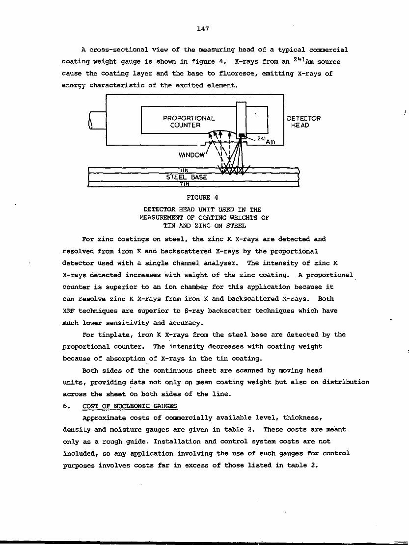
147
A cross-sectional view of the measuring head of a typical commercial
coating weight gauge is shown in figure 4. X-rays front an ^Am source
cause the coating layer and the base to fluoresce, emitting X-rays of
energy characteristic of the excited element.
\ PROPORTIONALCOUNTER
i y \ H !
_
yk241,\m
DETECTORHEAD
WINDOW'
TIN \,STEEL BASE
L^VA/XIX
TIN
FIGURE 4
DETECTOR HEAD UNIT USED IN THEMEASUREMENT OF COATING WEIGHTS OF
TIN AND ZINC ON STEEL
For zinc coatings on steel, the zinc K X-rays are detected and
resolved from iron K and backscattered x-rays by the proportional
detector used with a single channel analyser. The intensity of zinc K
X-rays detected increases with weight of the zinc coating. A proportional
counter is superior to an ion chamber for this application because it
can resolve zinc K X-rays from iron K and backscattered X-rays. Both
XRF techniques are superior to 3-ray backscatter techniques which have
much lower sensitivity and accuracy.
For tinplate, iron K X-rays from the steel base are detected by the
proportional counter. The intensity decreases with coating weight
because of absorption of X-rays in the tin coating.
Both sides of the continuous sheet are scanned by moving head
units, providing data not only on mean coating weight but also on distribution
across the sheet on both sides of the line.
6. COST OF NUCLEONIC GAUGES
Approximate costs of commercially available level, thickness,
density and moisture gauges are given in table 2. These costs are meant
only as a rough guide. Installation and control system costs are not
included, so any application involving the use of such gauges for control
purposes involves costs far in excess of those listed in table 2.

148
TABLE 2
APPROXIMATE COSTS OF LEVEL, DENSITY, THICKNESS AND MOISTURE GAUGES(1980 Australian Dollars)
Gauge Approximate Cost Comments
Level
Level
Fluid density
Thickness
Moisture
$1000 - 1200
$2500 - 5000
$3200 - 4000
$4000 +
$8000
Single point, on/off output,
Continuous monitoring; costdepends on length monitoredand complexity.
Cost depends on pipediameter.
Cost quoted for basicsingle point gauge.
Density-compensatedsurface backscattergauge.
7. BIBLIOGRAPHY
Cameron, I.F. & Clayton, C.G. [1971] - Radioisotope Instruments. Vol. 1,
Pergamon, Oxford.
Clayton, C.G. & Cameron, J.F. [1966] - Radioisotope Instruments in
Industry and Geophysics. IAEA, Vienna, p.15.
Watt, J.S. [1979] - Proc. IAEA Advisory Group Meeting on Practical
Aspects of Energy Dispersion X-ray Fluorescence Analysis.
IAEA, Vienna, p.216.

149
CHAPTER 5
X-RAY ANALYSIS
A Series of Lectures
L.S. Dale
R.A. Fookes
W.J. Howarth
J.S. Watt

151
PART A
INTRODUCTION TO X-RAY FLUORESCENCE (XRF) AND
X-RAY PREFERENTIAL ABSORPTION (XRA) ANALYSIS
by
L.S. Dale
J.S. Watt
153
1. INTRODUCTION
The next six lectures on X-ray analysis concentrate on radioisotope
analytical techniques. In general, X-ray tube techniques are more
widely known and understood in the mineral industry. Topics covered are •
as follows:
Introduction to X-ray fluorescence (XRF) and X-ray
preferential absorption CXRA) analysis including calculations.
Techniques for general purpose XRF and XRA analysis.
Techniques for on-stream analysis of mineral slurries.
On-stream analysis systems including plant experience.
Portable mineral analysers, bore core analysers and
in situ borehole analysers.
Radioisotope X-ray techniques of analysis are widely used in the
mineral industry. They are employed in the laboratory for analysis of
exploration, mining and concentrator samples; in the field for rapid
analysis of exploration and mine development samples, for in situ analysis
in boreholes during mining operations and for direct analysis at the
mine face; and in mineral concentrators for on-stream analysis of
mineral slurries.
Two commonly used methods for X-ray analysis of materials are X-ray
fluorescence (XRF) and X-ray preferential absorption (XRA). In XRF
analysis, the sample is irradiated with X-rays which cause the sample
atoms to fluoresce. The energies of these fluorescent X-rays are
characteristic of the atomic number (Z) of the atoms excited; hence the
concentrations of specific elements can be determined from measurements
of the intensities of their respective fluorescent X-rays.
In XRA analysis, the transmission of X-rays through the sample to
be analysed is usually measured at two X-ray energies bracketing the K
shell absorption edge of the element f> be determined (the wanted element).
The concentration of the wanted element is proportional to the difference
in transmitted intensities of the two energies.
2. BASIC X-RAY PRINCIPLES
The energy E of X-rays is related to the wavelength X :
E(keV) = 12.4/X
where X is in Angstrom units (A). In all of the X-ray lectures in this
course, X-rays are specified by energy rather than by wavelength.
When X-rays traverse matter they are attenuated by an amount dependent
upon the atomic number, thickness and density of the absorbing medium.
If a monochromatic beam of X-rays of energy E and intensity I is
154
incident upon a homogeneous absorber of thickness x, X-rays of intensity
I will pass through the absorber while the remainder (I -I) will be lostoby photoelectric absorption or scatter. The intensity of transmitted
photons, I, is not only proportional to I , but also dependent on variations
in thickness (dx) mass (dm) or number of atoms (dn) encountered by a
beam of cross section 1 cm2. If the proportionality constant is designated
y with a subscript x, m or n, the following relationships will hold:
dl = -I.y daxdl = -I.y dmmdl = -I.p dnn
The coefficients y,. y and y are called respectively the linear absorption•X/ HI H
coefficient, the mass absorption coefficient and the atomic absorption
coefficient. A simple relationship exists between these coefficients:
»x = V = V- N/A
where p is density, N is Avogadro's number and A is atomic weight.
The intensity of photons (I) traversing the absorber of thickness
x, without being scattered or absorbed, can be calculated by integrating
dl between the limits 0 and x. Hence, for example,
fcnl - fcnl = -y .xx o x
This equation is usually written as
-y par_ _ m1 = 1 exp
The mass absorption coefficient is the most useful of the three
absorption terms and it is common practice to refer to this simply as y.
The mass absorption coefficient is a function only of the energy of the
incident radiation and the atomic number of the absorbing element. The
mass absorption cofficient of any compound or composite material can be
calculated from the relationship:
y (compound) = E (y..W.)i * 1
where y. and W. are individual mass absorption coefficients and weight
fractions, respectively.
The X-ray energy region is loosely defined as 0.1-100 keV. In this
region, photoelectric absorption usually predominates over Compton
scatter. Coherent or Rayleigh scatter, which is highly forward directed
with no energy loss, can usually be neglected. The very large changes

ATOMIC NUMBER, Z
FIGURE 1
NARROW-BEAM ATTENUATIONOF GAMMA-RAYS
155

156
in total mass absorption coefficients in the X-ray region (figure 1) are
mainly due to changes in photoelectric absorption cross-section which,
per atom, is proportional to between Z**/A and Z5/A (A = atomic weight).
The Compton scatter cross section per acorn is proportional to Z/A
and hence approximately independent of atomic number (S/A - 1/2 except
for hydrogen). The energy loss on Compton scattering is usually small.
For example, energy losses for 90° scattering of 5, 20 and 100 keV X-
rays are, respectively, 0.05, 0.75 and 16.4 keV.
Radioisotope X-ray techniques are mainly used for the determination
of elements of Z > 20. There are two reasons for not using these techniques
for lower Z elements. First, fluorescent X-rays of low Z elements are
of very low energy and penetrate only thin layers of material. Preparation
of highly homogeneous samples is essential and this is time-consuming.
Secondly, the fluorescent yield 'u1 (the fluorescent X-rays emitted per
photoelectric absorption of X-rays by the appropriate shell) is low for
low Z elements, e.g. for the K shell X-rays <av = 0.11 at Z = 20, but atj\.Z = 92, w = 0.96 (figure 2). Hence with fewer fluorescent X-raysKemitted, sensitivity of analysis is worse.
10| 1 1 1 1 1 1 1 r
O9 -
OS
O7
3 O6-
3
205
O O 4
3 O3
O-2
K shellUK
shell
1O 2O 3O 4O SO 60 70 80 9OATOMIC NUMBER Z
FIGURE 2
RELATIONSHIP OF FLUORESCENT YIELDTO ATOMIC NUMBER
Figure 3 shows the binding energies of K and L shell electrons, and
the energy of K shell X-rays. The energy of fluorescent X-rays depends
on atomic number only and is independent of the energy of the X-rays
causing the atom to fluoresce. Hence the atomic numbers of elements in
the sample can be identified by measuring the energies of the fluorescent
X-rays emitted.

157rao
1 -too3 5 1 O 20 3 0
ATOMIC NUMBER.2
FIGURE 3
ELECTRON BINDING ENERGIES IN SHELLSAND AVERAGE K X-RAY ENERGIES
Appendix A gives data on K and L shell binding (absorption) energies
and fluorescent X-rays. There are two groups of K shell X-rays; the KQ
X-rays are lower in energy than K_ X-rays, and the relative abundance of
K :K0 is about 6:1.o pPhotoelectric absorption by an atom is the sum of the probabilities
of absorption by electrons in each electron shell. For this absorption
to occur, the incident X-ray must be of energy greater than that of the
binding energy of the particular electron. Most, but not all of the
absorption is by the electrons in the shell with binding energy just
below the energy of the incident X-ray. The ratio of K shell to total
absorption ?„ depends on atomic number and is shown in figure 4.1C
O-9
O-85
OL* O-8
O-75
O-7K> 2O 3O 4O SO 6O
ATOMIC NUMBER. Z70 8O 90
FIGURE 4
PROPORTION OF K-SHELL ABSORPTIONTO TOTAL ABSORPTION (PR) PLOTTED
AGAINST ATOMIC NUMBER (Z)

158
3. X-RAY FLUORESCENCE ANALYSIS
The basic principles of X-ray fluorescence (XRF) analysis [Jenkins
& De Vries 1967, Woldseth 1973] are given below. Figure 5 shows X-rays
incident on a sample interacting in a layer da; at a distance a: from the
sample surface, and the resultant K X-rays being detected by an X-ray
detector. The calculation of intensity of K X-rays detected from layer
dec is simplified by assuming that:
(a) photoelectric absorption is much greater than Compton scatter;
(b) the angle 0 is the same for incident and emergent X-rays; and
(c) the penetration of X-rays in the sample « the distances of
source to sample and sample to detector.
Sample dx(density*/0) i
4\TX
X-raysource
X-raydetector
FIGURE 5
PATH OF INCIDENT AND FLUORESCENTX-RAYS IN SAMPLE TO ILLUSTRATE
CALCULATIONS FOR X-RAY FLUORESCENCEANALYSIS
The intensity of detected K X-rays from layer da; is then given by :
_-JS. COS0
-— |exp~ (i)
where:
(a)
(b)
G is a calibration constant allowing for the X-ray emission
rate of the source, the detector efficiency, and the geometry
of the source, sample and detector;
exp [-E(y.W.)pa;/cos9] is the fraction of X-rays incident oni * i
the sample which reach da. y. and W. are, respectively, the1 ^ J.J.mass absorption coefficient and weight fraction of the i
chemical element in the sample. EW. = 1, and
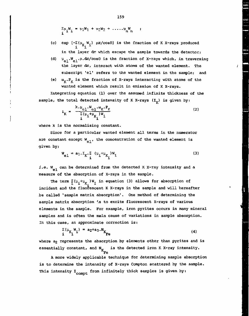
159
Ey.W. = • V Wn n
(c) exp [-I(y., W.) po;/cos6] is the fraction of K X-rays producedi Ki x
in the layer d»r which escape the sample towards the detector;
(d) p .W .p.dtf/cosQ is the fraction of X-rays which, in traversing6X 6.L
the layer dac, interact with atoms of the wanted element. The
subscript 'el1 refers to the wanted element in the sample; and
(e) W...P,, is the fraction of X-rays interacting with atoms of theJx is.
wanted element which result in emission of K X-rays.
Integrating equation (1) over the assumed infinite thickness of the
sample, the total detected intensity of K X-rays (I ) is given by:K.
(2)Z(y« -L1
)W. J-
where k is the normalising constant.
Since for a particular wanted element all terms in the numerator
are constant except W .,, the concentration of the wanted element is
given by;
i.e. W can be determined from the detected K X-ray intensity and aelmeasure of the absorption of X-rays in the sample.
The term Sdj.+yv )W. in equation (3) allows for absorption of1 2. K. 1
incident and the fluorescent K X-rays in the sample and will hereafter
be called 'sample matrix absorption'. One method of determining the
sample matrix absorption •'.s to excite fluorescent X-rays of various
elements in the sample. For example, iron pyrites occurs in many mineral
samples and is often the main cause of variations in sample absorption.
In this case, an approximate correction is:
E(yK Vi i- K
re (4)
where a£ represents the absorption by elements other than pyrites and is
essentially constant, and N,. is the detected iron K X-ray intensity.
A more widely applicable technique for determining sample absorption
is to determine the intensity of X-rays Compton scattered by the sample.
This intensity I from infinitely thick samples is given by:

160
ycompt i(5)
where G is a calibration constant and the subscript 'compt1 refers to
Compton scattering, and y. is the same as in both equations (3) and (5).
Although y 7* y , they are approximately proportionally related.i " i
Hence from equations (3) and (5)
IW 1 ~ aif I ^compt
This technique is widely used in many analysis applications in the
mineral industry, e.g. for on-stream analysis of mineral slurries and
for analysis of samples using portable mineral analysers.
In the above discussion it has been assumed that the sample is
homogeneous, since sample non-uniformities and variations in particle
size affect the accuracy of analysis. Grinding the sample to prepare it
for analysis is" not necessary for many applications. A rough rule of
thumb is that particles of size less than 0.693/(yp) are required, where
y is the mass absorption coefficient of incident or emerging X-rays.
4. X-RAY PREFERENTIAL ABSORPTION ANALYSIS
X-ray preferential absorption (XRA) analysis is normally used to
determine the concentration of a high-Z element in a sample of lower-Z
matrix elements. Typical elements determined include uranium, bismuth,
lead and tungsten.
Referring to figure 6, transmission measurements of highly collimated
beams of X-rays are usually made at X-ray energies above (H) and below
(L) that of the K-shell absorption-edge energy of the element to be
determined. At each energy, the intensity I of X-rays transmitted by
the sample is related to the intensity I measured with no sample present
by
— =expi-Z(y.W.)pacV| v (7)
If the wanted element (el) has subscript '!' and is separated from the
rest of the sample matrix, then equation (7) can be rewritten
(8)

161
-Radioisotopesource
--Source• collimator
Sample
Detectorcollimotor
Scintillationdetector
FIGURE 6
GEOMETRY FOR X-RAY ABSORPTIONANALYSIS
In some cases, a single measurement of transmission at an X-ray
energy higher than the K edge of the wanted element is sufficient ton
determine W . This is when Z y.W. is approximately constant. I and I
are measured, and the weight per unit area px is determined by weighing
a known cross-sectional area of sample. Then
Wel(9)
In more complex cases, separate measurements with X-rays higher and
lower in energy than the K edge energy are made. In this case:
Wel (ytt
_
elj -el(i *» (Hi - 10'(r)J (10)
If both X-ray energies are essentially the same and bracket the K edge,
ag - 1. Accurate analysis can often be made in spite of the use of
energies not close to the absorption edge. However, the accuracy is
affected if'another element has a K edge also bracketed by the two X-ray
energies.

162
5. CONCLUSION
The principles of X-ray analysis have been introduced to provide a
background to enable appreciation of its application in the mineral
industry. These applications are discussed in subsequent lectures.
6. BIBLIOGRAPHY
Jenkins, R. & De Vries, J.L. [1967] - Practical X-ray Spectrometry.
Philips Technical Library, Eindhoven.
Woldseth, R. [1973] - X-ray Energy Spectrometry. Kevex Corporation,
Burlingame, California.

163
APPENDIX A
X-RAY CRITICAL ABSORPTION ANDEMISSION ENERGIES (keV)
By S. FINE and C. f, HENDEE *Phihpt Laboratories
on Hudson, \ew York
Increased use of energy-proportionaldetectors for X-rays has created a needfor a table of energy values of K andL absorption and emission series.
The table presented here includesall elements. Most values were ob-taine by a conversion to kev of tabu-lated xperimental wavelength values(1-3) ; some are from previous energy-value compilations (4, 5). Where achoice existed, the value chosen wasthe one derived from later work. Cer-tain values were determined by inter-polation, using Moseley's law. (Allthis is annotated in footnotes.)
The conxfiMtia <.-i|ii.itiuiis rt-l.ttingenergy and wavelength used are (6)
E (kev) = (12.3%44 x 0.00017;, \iA)= 12.39644 1.002020 X(kX unit)
In computing values the number ofplaces retained sufficed to maintain theuncertainty in the original source value.The values in the table have been listeduniformly to 1 ev. However, chemicalform may shift absorption edges asmuch as 10-20 ev (4, 5).
To discover computational errors afit was made to Mnselcy's law. Ingeneral the values were consistent,however there were a few inc-gularitiesdue to the deviation of some inputvalues (/). These were retained in the
body of the table but a set of valuescalculated to fit better are footnoted.
« * *The authart itiih to ezpreti their apprecia-
tion to H*. ParrilHfer helpful luggeitioni andto //. Kaiper for performing the computationin connection with thit work-
BIBLIOGRAPHY
/. V. Caucboia. H. Huluhei. "Table* de Con-atantes et Donneea Numerique*. I. Longueur*D'Onde d«* Emiaaiona X et de* Diecominuite*D'AUorpuon X" (Hermann et Cie. Pari*France. 1947)
t. A. H. Compton and S. K. AUiaon. "X-ray* inTheory and Experiment" (D. Van NoatrandCo.. Inc.. New York, 19S1)
3. C. E. Moore. "Atomic Energy Level*." NBS487 (National Bureau of Standard*. U. S.Department ol Commerce, Waahmgton. D. C.,1949)
4. V. Cauchoia. J. p*v». radium 13, 113 (19S2)f. H. D. Hill. E. L. Cburcb. and J. W. Mibelieb.
Rn. Set Inttr. »J. 523 (1952)d. J. W. :... DuMond. E. R. Cohen. PAyi. Am.
81, 555 (1951)
X-Ray Critical-Absorption and Emission
AtomicNum-
ber Element
123456789
101112131415161718192021222324252627282930
HydrogenHeliumLithiumBerylliumBoronCarbonNitrogenOxygenFluorineNeonSodiumMagnesiumAluminumSiliconPhosphorusSulphurChlorineArgonPotassiumCalciumScandiumTitaniumVanadiumChromiumManganeseIronCobaltNickelCopperZinc
Energies in kev
K tenet
/C.b Kft, A
0.0136{0.0246*0 0550.116$0. 19 f0.28U0.3990.5310.687t0.874*1.08* 11.303 11.559 11.838 12. 142 22.470 22. 81911 23.203 33.6074.0384.4964.9646.4636.9886.5377.1117.7098.3318.9809.660
344
-4-5-5
677
8.328 88.976 89.657 9
.067
.297
.553
.832
.136
.464
.815
.192$
.589
.012
.460
.931
.427
.946
.490
.057
.649
.264
.904
.571
A'ai A'a: i-Uh
0 0520 1100 1850 2820 3920 5230.6770 851$ 0 048t1.041 0 055$1.254 0 063
1.487 1 486 0.0871 740 1.739 0 118*2.015$ 2 014$ 0 153*2.308 2.306 0.193*2.622 2.621 0.238*2.957 2.955 0.287*3.3133.6914.0904.5104.9525.4145.8986 4036.9307.4778.0478.638
3 3203.6884.0854.5044.9445.4055.8876.3906.9157.4608.0278.615
0 341*0 399*0.462*0.530*0.604*0.679*0.762*0.849*0.929*1.015*1.100*1.200*
L teriet
£iub /'itub ^-Ti Lft Wi Loi Lot
0.022t0.034$0.0500.073**0 099**0.129$0.164**0.203$0.247**0.297**0.3520.411**0.460**0.519**0.583**0.650**0.721**0.794**0.871**0.9531.045
0.022f0 034$0.0490.072**0.098**0.128$0. 163**0.202$0.245**0.294**0.3490.406**0.454**0.512**0.574**0.639**0.708**0.779**0.853**0.9331.022
0.3440.3990.4580.6190.5810.6470.7170.7900.8660.9481.032
0.3410.3950.4520.6100.5710.6360.7040.7760.8490.9281.009
*Nucleonics, 13(3)36, 1955
(Continued)

164
AtomicNum-
ber Eltmtnt
313233343536373839404142434445464748495051525354555667585960616263646566676869707172737475767778798081828384858687888990919293949696979899
100
GalliumGermaniumArsenicSeleniumBromineKryptonRubidiumStrontiumYttriumZirconiumNiobiumMolybdenumTechnetiumRutheniumRhodiumPalladiumSilverCadmiumIndiumTinAntimonyTelluriumIodineXenonCesiumBariumLanthanumCeriumPraseodymiumNeodymiumPromethiumSamariumEuropiumGadoliniumTerbiumDysprosiumHolmiumErbiumThuliumYtterbiumLuteciumHafniumTantalumTungstenRheniumOsmiumIridiumPlatinumGoldMercury•ThalliumLeadBismuthPoloniumAstatineRadonFranciumRadiumActiniumThoriumProtactiniumUraniumNeptuniumPlutoniumAmericiumCuriumBerkeliumCalifornium
A'.b
10.36811.10311.86312 65213 47514.32315.20116. 10617.03717 99818 98720.00221.054$22.11823.22424.34725.51726.71227.92829.19030 48631.80933 16434 57935.95937.41038.93140 44941 99843.57145 207$46.84648.51550 22951.99853.78955.61557.483
A" series L stria
A fit A'jJi A'ai A'ai Lub /-u»b
10.365 10 263 9 251 9 234 111.100 10 981 9 885 9.854 111.863 11.725 10 543 10 507 112.651 12.495 11 221 11. LSI 113465 13.2'JO 11 <<-M 11.S77 t14 313 14.112 12 t>4!> I 2. 597 115.184 14.9GO 1331)4 13335 216 083 15.834 14 164 14.097 217 Oil It! T.»ti H »jr I I . Afl- -17.969 17.666 15.774 15.690 218.951 18.621 IB 014 16 520 219.964 19.G07 17.478 17.373 221.012$-20 5851 18 4101 IS 3281 322.072 21.655 19278 19.149 323.169 22.721 20.214 20 072 324.297 23.816 21 175 21 018 325454 24.942 22.102 21 !>S8 326641 26.093 23.172 22982 427.859 27.274 24 207 24 000 429.106 28 483 25 270 25 042 430 387 29 723 26 357 20 109 431 698 30.993 27 471 27 200 433 016 32 292 28 010 -J8 :«l.r> 534 4461 33 644 29 8021 29 4H5C 535 819 34 984 30 970 30 623 537.255 36.376 32 191 31 815 538 728 37.799 33 440 33 033 fi40 231 36.255 34 717 34 270 (i41 772 40 746 36 023 35 5-18 643 2985 42 269 37 359 36 .S45 744 955$ -43. 9451 38 649C 38 lf.0c 746 5531 45.400 40.124 39 523 748 241 47.027 41 529 40.877 849 961 48 713 42 983 42 280 851.737 50.391 44.470 43.737 S53491 52178 45.985 45.193 955 292** 53.934$ 47.528 46.GS6 957.088 55.690 49.099 48.205 9
59.3351 58.969** 57.5761 50 V30 49 762 1061.30363.30465.31367.40069.50871.66273.86076.09778.37980.71383.10685.51788.00190.52193.11295.74098.418
101.147103.927106.759109.630112.581115.591118.619121.720124.876128.088131.357134.683138.067141.510
60 959 59.352 52 360 51 326 1062.946 61.282 54.063 52 959 1064.936 63.209 55.757 54.579 1166 999 65.210 57.524 56.270 1169 090 67.233 59.310 57.973 1271 220 69.298 61.131 59.707 1273.393 71.404 62.991 61.477 1275.605 73.549 64.886 63.278 1377.866 75.736 66.820 65.111 1380.165 77.968 68.794 66.980 1482.526 80.258 70.821 68.894 1484.904 82.558 72.860 70.820 1587.343 84.922 74.957 72.794 1589.833 87.335 77.097 74.805 1692.386 89.809 79.296 76.868 1694.976 92.319 81.525 78.956 1797.616 94.877 83.800 81.080 18
100.305 97.483 86.119 83.243 18103.048 100.13d 88.485 85.446 19105.838 102.846 90.894 37.681 19108.671 105.592 93.334 89.942 20111.575 108.408 95.851 92.271 21114.549 111.289 98.428 94.648 21117.533 114.181 101.005 97.023 22120.592 117.146 103.653 99.457 23123.706 120.163 106.351 101.932 23126.875 123.235 109.098 104.448 24130.101 126.362 111.896 107.023 25133.383 129.544 114.745 109.603 25136.724 132.781 117.646 112.244 26140.122 136.075 120.598 1M.926 27
30* 142* 1529 1C>52 17!Ǥ 1<.).<!$ 1007 1221 2M3 -
.547 2
.700 2
.RS4 2054$ 2
.236$ 241!) 3B17 3810 3019 3•J37 3104 4
097 4038 4I'll) 4452 5720 5
.995 5283 5501 0S40 ti
.144 6448$ 7754 7069 7393 7
.724 8083 8411 8776 «
.144 9486 9867 10-'04 10
.676 11090 11
.522 11
.965 12
.413 12
.873 13
.353 13
.841 14
.346 14870 15
.893 15
.935 16
.490 16
.058 17
.638 17
.233 18
.842 19
.460 19
. 102 20
.753 20
.417 21
.097 22
.793 22
.503 23
.230 24
.971 25
.729 25
.503 26
134**24S**3594735!iy«*7JT«*8GC
.008jjl3054«7*«G277!>S$900145329528727039157381C13s")0104358623894
. HiSt443727
.018$281*i
.624!MO2586211920263
.628977
.345
.734
.130
.535
.955
.383
.819
.268
.733
.212
.697
.207
.716
.244
.784
.337.904.481.Q78.688.311.943.596.262.944.640.352.080.824.584
Liiub /
1 117**1.217**1.3231 434i :.52»*1.075**1.8061.941- ors2.220 22 374 22.523 22 677$ 2•J 837 23 002 33.172 33 352 33 538 33 729 33 '.128 44 132 44 341 44 559 44 7hJ 55 Oil 55 247 55 489 55 729 05.90H G6.215 66.466§ 66.721 76.983 77 252 77.519 87.8501 88 074 88 364 98 652 98.943 99 241 109.556 109.876 10
10 198 1110 531 1110 869 1211.211 1211.559 1211.919 1312.285 1312.657 1413.044 1413.424 1513.817 1514.215 1614.618 1615.028 1715.442 1715.865 1816.296 1816.731 1917.163 2017 614 2018.066 2118.525 2218.990 2219.461 2319.938 2420.422 2420.912 25
,-n L0, LfJ,
302 2402 2623 2792$ 2964 2144 3328 3519 3716 3920 3131 3347 4570 4SOO 4036$ 4280 4531 5789 5052 5322 5602 6891$ 6ISO 6
.478 6788 7
.104 7
.418 7
.748 7
.089 8
.424 8779 8
.142 9
.514 9892 9
.283 9
.084 10
.094 10
.509 10
.939 11
.379 11
.828 11
.288 12
.762 12
.244 12
.740 13
.248 13
.768 14
.301 14
.845 14
.405 15
.977 15
.559 16
.163 16774 16
.401 17
.042 17
.699 18
.370 18
.056 18
.758 19
.475 19
11111I11J
.219 2367 2518 2674$ 283G 2001 2172 2348 3528 3713 3904 3100 3301 4507 4720$ 4936 4156 4384 5613 5
.850 5
.090 5336$ 5
.587 6
.842 6
.102 6
.368 6G38 7
.912 7
.188 7
.472 8758 8
.048 8346 9
.649 9
.959 9
.!"3 10
.596 10
.918 10
.249 11
.582 11
.923 11
.268 12
.620 12
.977 13
.338 13
.705 13
.077. 14
.459 14
.839 15
.227 15
.620 16.022 16.425 17.837 17.254 18.677 18.106 19.540 19.980 20.426 21.879 21
122216317419526
La, La,
.096
.186282
.379
.480.tKS»$ 1.587**.752.87295S
.124257395538$683834990151316487662843029220
.422$620828043262489722956206
.456714
.979
.249
.528
.810
.103401
.708
.021
.341
.670
.008
.354
.706
.069
.439
.823
.210
.611
.021
.441
.873
.316
.770
.233
.712
.200
.700
.218
.740
.278
.829
.393
.971
.562
.166
.785
1.6941.806J !>222.0422 1662 2932.424$2 5582 6962 8382 '.1843 1333.2873 4443 6053 7693 9374 111$4.2864 4674 6514 8405.0345.2305.4315.6365 8466 0596.2756.4956.7206.9487.1817.4147.6547 8988.1458.3968.6518.9109.1739.4419.7119.987
10.26610.54910.83611.12811.42411.72412.02912.33812.65012.96613.29113.61313.94514.27914.61814.96115.30915.66116.01816.379
1.69'l.SOoJ 9-02.0403 1632.2902 420$2.5542 6922 8332.9783 1273.2793.4353.5953.7583 0264.098$4.2724.4514.G354.8235.0145.2085.408$5 6095.8166 0276 2416.4576.6806.9047.1357.3677.6047.8438.0878.3338.5848.8409.0989.3609.6259.896
10.17010.44810.72911.01411.30411.59711.89412.19412.49912.80813.12013.43813.75814.08214.41114.74315.07915.42015.76416.113
For Z ^ 69, value* without lymbol* are derived from (/). Value* prefixed with a - *ign are K/>u».For Z £ 70. abaorption-edgo value* are from (4) in tbe cat* of Z - 70-83. 88. 90. and 92; remaining absorption edge* to Z - 100 are obtained from the**
by leaat-iquare* quadratic fitting. All emiarion value* for 2 ^ 70 are derived from tbe preceding abeorption edge*, and other* baaed on U), using the transi-tion relation* K<n m JT», - LIU. Ka» m *»b - In. Ktt - K.b - Min. etc.
• Obtained from R, D. Hill. E. L. Church. J. W. Mibelieh <«. f Derived from Compton and Alliioo (t). I Derived from C. E. Moor* (J).IValue* derived from Caucbois and Hulubei (t) which deviate from the Moseley law. Better-fitting value* are: Z - 17, /t.b - 2.826; Z - 43,
JCat - 18.370. JCai - 18.250. Kfi - 20.612; Z - 54. Kai - 29.779, Ka, - 29.463, Kff, - 34.398; Z - 60. Ktt - 43.349; Z - 61. Ku> m 38.720. Ka, -38.180. JWi - 43.811; Z - 62. Kft - 46.581. Lj, - 7.312; Z - 66. Ln - 8.591. tut - 7.790; Z - 69. K.b - 59.382. Kf\ - 57.487.
I Calculated by method of least squares. ** Calculated by transition relations.

165
PART B
TECHNIQUES FOR GENERAL PURPOSE
XRF AND XRA ANALYSIS
by
R.A. Fookes
J.S. Watt

167
1. INTRODUCTION
Techniques for XRF analysis are based on the use of solid-state,
scintillation and proportional detectors. The techniques are different
for each type of detector because of their large differences in resolving
power for X-rays (figures 1 and 2). Solid-state detectors resolve K X-
rays from elements of adjacent atomic nussber (Z), hence element concentration
is obtained by simple signal processing. Proportional counters (high
resolution) have worse resolving power which results in some spectral
overlap in K X-rays from adjacent Z elements, hence more complex spectral
processing is required. Scintillation detectors cannot resolve adjacent
Z elements so analysis combines coarse spectral analysis to separate
fluorescent from backscattered X-rays with the use of X-ray filters to
isolate the K X-rays. The techniques of XRF analysis with each of the
three types of detectors are discussed, as well as XRA analysis based on
use of scintillation detectors.
>•t 4£UJ
I 3UJ
1 *HIat
Koi X-roys L she" X-rogsFeCoNiCuZn Pb Pb
Scintillolion
Proportionol4
normalhigh resolution
- Solid stole
0 2 4 6 8 !0 12 14E N E R G Y ( k e V )
FIGURE 1
RESOLUTION OF X-RAY DETECTORS FORCOPPER Kpj X-RAYS ILLUSTRATED IN
RELATION TO ENERGIES OF FLUORESCENTX-RAYS OF SOME ELEMENTS COMMONLYDETERMINED IN ON-STREAM ANALYSIS
10 eV
PHOTON ENERGY (keV)
FIGURE 2
ENERGY RESOLUTION OF DETECTORS ANDADJACENT ELEMENT K^ X-RAY PEAK
SEPARATION
Radioisotope X-ray sources most commonly used with the above detectors
are 55Fe, 238Pu or its alternative 2'*'fCm, 21tlAm and 57Co. The physical
properties of these and several other useful sources of X-rays are given
in table 1. Also given are ranges of elements which can be excited with
each radioisotope.

168
TABLE 1
PHYSICAL PROPERTIES OF RADIOISOTOPES USED INNON-DISPERSIVE X-RAY FLUORESCENCE ANALYSIS
Radioisotope
55Fe
238Pu
Cm109
Cd
125I
153Gd
Am
57Co
Half-life(years)
2.7
86
17.6
1.3
0.16
0.65
458
0.74
Photon Emission
keV
5.9-6.5 (Mn K X-rays)
13.6-20 (u L X-rays)
14-21 (Pu L X-rays)
22-25 (Ag K X-rays)
88
27-31.7 (Te K X-rays)
35
41-47 (Eu K X-rays)
97
103
59.5
13. 7-20. 8 (Np L X-rays)
122
136
%
28.5
13
10
107
4
138
7
90
30
20
37
37
89
8.8
Elements Excited
K X-rays L X-rays
Al-V
Ti-As Nd-Bi
Ti-As Nd-Bi
Ti-Mo Nd-U
Fe-Ag Nd-U
Pr-Bi As-Ce
As-Tm
Nd-U
2. XRF ANALYSIS USING SOLID STATE DETECTORS
2.1 General Comments
Solid-state detectors are mainly used to analyse mineral samples in
the laboratory [Woldseth 1973, Gravitis et al. 1974], but they are in
limited use for on-stream analysis. The main advantage is that their
high resolution enables simultaneous multi-element analysis with excellent
sensitivity. Minimum detectable levels are, for Z £ 24, about 20-50
parts per million (ppm). Analysis for low Z elements, e.g. silicon and
aluminium is also possible but considerable sample preparation is essential
to ensure homogeneous samples.
A simple laboratory system comprising solid-state detector, radioisotope
X-ray source and electronics, including a multichannel analyser, costs
about US$25 000. The most complex system comprising detector, X-ray

169
tube, and computer processing of signals to give a print out of wanted
elements costs about US$100 000. A supply of liquid nitrogen is essential
for adequately cooling the detector (Si or Ge).
2.2 Example
A typical arrangement iGravitis et aJL. 1974] of radioisotope X-ray
source, sample, and solid-state detector is shown in figure 3. The
spectrum of X-rays from a copper tailings sample is shown in figure 4.
The sample was excited by a <3pu source which emits uranium L X-rays
(mainly 13.6, ~ 17 and 20 keV). The scattered X-ray peaks result from
Compton and coherent scattering of the uranium L X-rays in the sample.
The energies of the fluorescent X-rays indicate the presence of iron,
copper and arsenic in the sample. The low energy K X-rays from the low
Z elements such as sulphur (Z = 16) arc not visible because they are
inefficiently produced (i.e. u is low) and are strongly absorbed in both
the sample and the window between sample and detector.
Preomplifierinput stage
CnjQstot..
Vacuum -
To liquid —nitrogen
—Sample
-*— Radioisotopesources
Berylliumwindow
^ Silicondetector
—Leads topreamplifier
0 1 2 3cm
01
a:
Oo
Sample containsFe-4-8%Cu- 0-14%As-O- l
Fe CuT f BockscotteriAs *- — i
FIGURE 3
10 15X-RAY ENERGY (keV)
FIGURE 4
20
HEAD ASSEMBLY SHOWING RADIOISOTOPEX-RAY SOURCES AND SOLID STATE DETECTOR
SPECTRUM OF X-RAYS EMITTED BY COPPERTAILING SAMPLE FROM MOUNT ISA MINES LTD
WHEN EXCITED BY X-RAYS FROM A238Pu RADIOISOTOPE SOURCE
Figure 5 shows measurements made on solid samples of flotation
feeds tjken from three mineral concentrators. For samples from the same
concentrator, the copper K X-ray intensity is an approximate measure of
copper content (figure 5). However, there is essentially no overlap
with samples from the other concentrators. This shows thac the absorption
of X-rays in the matrix of samples from different concentrators is widely
different. Iron is the main cause of matrix absorption in these feed
samples. The iron content for Bougainville, Cobar and Peko feeds averages
about 5,20 and 50 wt% respectively. When allowance is made for matrix
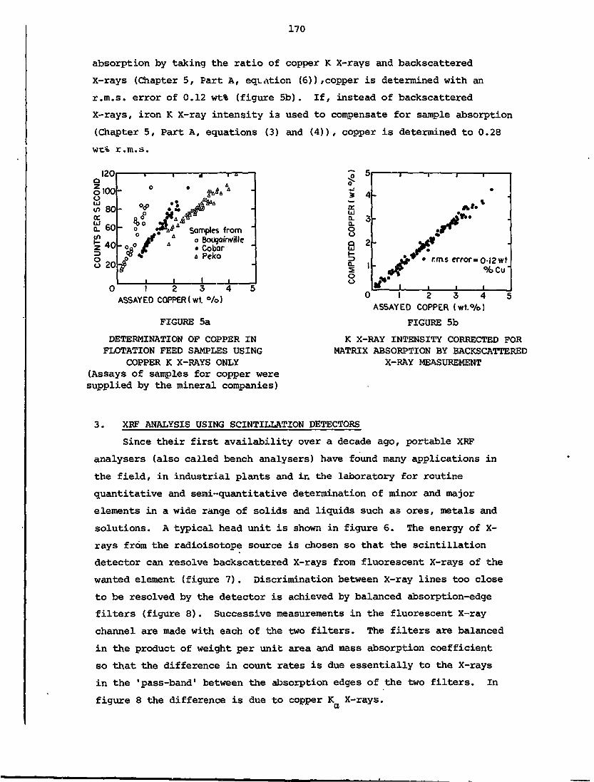
170
absorption by taking the ratio of copper K X-rays and backscattered
X-rays (Chapter 5, Part A, equation (6)),copper is determined with an
r.m.s. error of 0.12 wt% (figure 5b). If, instead of backscattered
X-rays, iron K X-ray intensity is used to compensate for sample absorption
(Chapter 5, Part A, equations (3) and (4)), copper is determined to 0.28
wc% r.m.s.
olOOuQJ<n 80-(E
^60
8 20
°rf>o
Samples fromo Bougainville• CobarA Peko
10 1 2 3 4 5
ASSAYED COPPER (wt. %)
FIGURE 5a
DETERMINATION OF COPPER INFLOTATION FEED SAMPLES USING
COPPER K X-RAYS ONLY(Assays of samples for copper weresupplied by the mineral companies)
£ia:QJa.a.88Q.5oo
o
4
3
2
|I
I 1
.
m
*1
Xjyp • r,m.stf*u^
^M0
if ,
1 1
'
.****jA*»«PPi
error= 0-12 wt%Cu'
, i0 1 2 3 4ASSAYED COPPER (wt.%)
FIGURE 5b
K X-RAY INTENSITY CORRECTED FORMATRIX ABSORPTION BY BACKSCATTERED
X-RAY MEASUREMENT
3. XRF ANALYSIS USING SCINTILLATION DETECTORS
Since their first availability over a decade ago, portable XRF
analysers (also called bench analysers) have found many applications in
the field, in industrial plants and in. the laboratory for routine
quantitative and semi-quantitative determination of minor and major
elements in a wide range of solids and liquids such as ores, metals and
solutions. A typical head unit is shown in figure 6. The energy of X-
rays from the radioisotope source is chosen so that the scintillation
detector can resolve backscattered X-rays from fluorescent X-rays of the
wanted element (figure 7). Discrimination between X-ray lines too close
to be resolved by the detector is achieved by balanced absorption-edge
filters (figure 8). Successive measurements in the fluorescent X-ray
channel are made with each of the two filters. The filters are balanced
in the product of weight per unit area and mass absorption coefficient
so that the difference in count rates is due essentially to the X-rays
in the 'pass-band' between the absorption edges of the two filters. In
figure 8 the difference is due to copper K X-rays.

FIGURE 6
A SOURCE-DETECTOR ASSEMBLY FORANALYSIS OF SLURRIES USINGRADIOISOTOPE X-RAY TECHNIQUES
FIGURE 7
TYPICAL SPECTRUM OF X-RAYS FROM ACOPPER ORE SLURRY EXCITED BY X-RAYSFROM 238Pu AND MEASURED USING A
SCINTILLATION DETECTOR
X- RAY ENERGY (keV)
FIGURE 8
X-RAY TRANSMISSION THROUGH BALANCEDFILTERS OF NICKEL AND COBALT.
Fe K, Cu K AND AS K X-RAY ENERGIES SHOWN

172
The advantages of balanced filter techniques using scintillation
detectors are that equipment used is very simple and inexpensive (~US$10 000),
and that portable equipment can be made very robust for use in the
field. The sensitivity is adequate for many practical applications.
Minimum detectable levels for very favourable cases can be as low as
50 ppm, but usually they are in the range 100 to 300 ppm. Multi-element
analysis is probably unpractical because it would require a mechanically
complex filter changer with two filters for each element to be determined.
Many of the practical applications of these mineral analysers have
been summarised by Rhodes [1971].
4. XRF ANALYSIS USING PROPORTIONAL DETECTORS
Recent developments in proportional detectors have led to a moderate
improvement in X-ray resolution [Sipila & Kiuru 1978], e.g. for copper
K X-rays (8 keV) from 16 per cent FWHM to 10 per cent. This improvement
allows the error in copper and zinc determination (in a sample with 0.1
per cent Cu and 0.1 per cent Zn) to be reduced from about 40 per cent to
5 per cent relative. Energy resolution is now sufficient to enable
adjacent elements to be measured simultaneously if their concentrations
are similar. In practice, counts between the FWHM of the fluorescent
X-ray spectral peaks are measured and corrections made for the overlap
X-ray peaks from adjacent elements. This is done electronically, using
an analogue-to-digital converter and a microprocessor. Corrections for
sample matrix absorption are made using the measured intensity of
back-scattered X-rays.
The above system [Rautala et al. 1979] can be used for the simultaneous
determination of up to about four close Z elements. Sensitivity and
accuracy are about the same as for scintillation detectors for elements
of Z > 25, and considerably better for lower Z elements. The overall
system costs US$20 000 and is preferred to scintillation detector analysers
!' for determination of low Z elements or when simultaneous multi-element
j determination is necessary. The equipment can be made portable and
i hence can be used in the field or at the mineface.ij 5. XRA ANALYSIS USING SCINTILLATION DETECTORS
X-ray preferential absorption (XRA) analysis, based on use of
highly collimated beams of X-rays or low energy X-rays, is used to
determine concentrations of high-Z elements such as uranium, bismuth,
lead and tungsten. Scintillation detectors are universally used for XRA
analysis because resolving power is not important and these detectors

173
are simple and efficient at high X-ray energies. Equipment is similar
to that used for portable mineral cuidlyscas, but Lhe head unit is set up
for transmission rather than XKP (figure 9). The cost for laboratory or
portable equipment is about US$10 000. Minimum detectable levels are
about 50-500 ppm depending on the application.
--Rodioisotopea \.
. .-Sourcecollimolor
Sample
Detectorcol 11 mo tor
. Scintillationdetector
FIGURE 9
GEOMETRY FOR X-RAY ABSORPTION ANALYSIS
An example of XRA analysis [Ellis et al. 1969] is the determination
of the lead concentration of ores and ore products. Separate collimated
beam transmission measurements were made with 153Gd (~100 keV) and 2tflAm
(59.5 keV) which bracket the energy of the lead K absorption edge (88.1 keV)
Figure 10 shows results for 153Gd transmission alone in zinc concentrates
and residues, and then the result of combining the 153Gd and 2iflAm
measurements. The r.m.s error of 0.04 wt% is achieved in spite of the
great difference in sample matrix absorption, and in spite of the energies
of X-rays being far from the energy of the lead absorption edge.

174
70
65
o 6O
zQ 55
2(A
50-
45
4O
35
Residues. approx. O-6wt. °/o zinc
Zinc concentrates:approx.53 wt °/o zinc
1-4
1-2
I-O-
o••-»IB
I 04
8
r.m.s. error: O-O4wt.°/o-lead
O O-2 O-4 O-6 O-8 I-O 1-2
LEAD (wt.°/o)
(a) 153Gd transmission (T)
1-4 O O-2 O-4 O-6 O-8 I-O 1-2 1-4
LEAD(wt. °/o)
(b) T is compensated by 21tlAm(60keV) y-ray transmission
FIGURE 10
DETERMINATION OF LEAD IN ZINC CONCENTRATES ANDRESIDUES, SHOWING HOW COMPENSATION REDUCES THE
EFFECT OF SAMPLE MATRIX VARIATIONS
6. BIBLIOGRAPHY
Ellis, W.K., Fookes, R.A., Gravitis, V.L., Watt, J.S. [1969] - Radioisotope
X-ray Techniques for On-stre.am Analysis of Mineral Slurries.
Int.J.Appl. Radiat.lsot., 20:691.
Gravitis, V.L., Greig, R.A. & Watt, J.S. 11974] - X-ray Fluorescence
Analysis of Mineral Samples usring solid-state detector and Radioisotope
X-ray'Source. Proc.Aust.Inst.Min.Metall., 249:1.
Rautala, P., Hietala, M. & Sipila, H. [1979]. - Application and Economical
Aspects of WDXRF and EDXRF Techniques in Industry. In Practi cal
Aspects of Energy Dispersive X-ray Emission Spectrometry. IAEA-216,
pp. 119-134.
Rhodes, J.R. [1971] - Design and Application of X-ray Emission Analysers
using Radioisotope X-ray and Gamma-ray Sources. American Society
for Testing and Materials (ASTM) Special Technical Publication 485.
Sipila, H. & Kiuru, E. [1978] - On Energy Dispersive Properties of the
Proportional Counter Channel. In Advances in X-ray Analysis',
Vol. 21 (Ed. Barrett, C.S. et al), Plenum Press, New York.
Woldseth, R. [1973] X-ray Spectrometry. Kevex Corporation, Burlingame,
California.

175
PART C
X-RAY TECHNIQUES FOR ON-STREAM ANALYSIS
OF MINERAL SLURRIES
by
R.A. Fookes
J.S. Watt

177
1. INTRODUCTION
On-stream analysers have been developed to provide information for
the more effective and efficient control of mineral concentration processes.
Continuous or frequent determination of mineral concentrations in various
streams, to give correct indication of trends, is far more important for
process control than exact but infrequent instantaneous analyses. The
normal requirements of analysis are for the concentrations of one or two
elements per process stream.
The development of on-stream analysis systems based on'the X-ray
tube and Bragg crystal spectrometer began in the 1950s. Such spectrometers
are too complex and expensive for normal on-line use, and so are operated
in a laboratory centrally located in the plant. They sequentially view
slurries sampled from various process streams and routed through long
runs of small diameter pipe to the analyser. The main problems associated
with these early systems were pipe blockages and the difficulty of obtaining
truly representative samples of process streams. By the leite 1960s,
reliable but expensive and relatively complex systems became commercially
available, typically analysing sequentially about 14 process streams
with a cycle time of about 7 minutes [Leskinen et al. 1973, Basinger 1973].
Radioisotope X-ray techniques of analysis were also developed in
the 1950s, the first applications being for the analysis of solutions
containing elements of high atomic number, such as uranium. These
techniques had potential for normal on-line use because head units
containing the source and detector were relatively inexpensive and could
be mounted adjacent to each stream. However, unlike analysers based on
the crystal spectrometer, the radioisotope techniques were not sufficiently
sensitive or selective to the specific element for most practical applications.
These limitations were overcome mainly in the 1960s [International Atomic
Energy Agency 1970] and radioisotope on-stream analysis systems are now
available commercially and in routine use in mineral concentrators [Watt
1977] .
The reliable on-stream analysis systems of today have benefited greatly
from advances in detectors, electronics, computers and microprocessors.
The trend in development of analysis systems is towards the use of
higher resolution detectors, more complex processing of signals from the
detectors, continuous analysis of each process stream, and the location
of detector head units in or close to the process streams so as to avoid
or minimise sampling. Present systems are sufficiently accurate for
process control but not for metallurgical accounting.

178
X-ray techniques used in on-stream analysis systems are now described,
followed by an outline of some commercially available systems, including
sample presentation, installation and plant operating experience, and
economic savings achieved. The term 'in-stream' refers to analysis
probes immersed directly in the plant process stream; the alternative is
to sample the stream continuously and route the sampled slurries in a
by-line to the analyser. 'On-stream' refers to the general case of
analysis with either system.
2. X-RAY TECHNIQUES
X-ray fluorescence (XRF) is the most widely used on-stream analysis
technique, with Y~raY preferential absorption being limited to some
analyses for elements of atomic number (Z) greater than 70, such as lead
and uranium. In XRF analysis, measurements are made of the intensities
of fluorescent X-rays of the wanted element and, usually, X-rays backscattered
by the slurry. The latter measurement is used to correct the variations
in absorption of X-rays by the slurry with change in composition of
solids matrix. The requirement for on-stream analysis is concentration
of the wanted element in the slurry solids; this is obtained by combining
the X-ray measurements with a measurement of the weight-fraction of
solids in the slurry. The solids weight-fraction is determined from a
measurement of either y~*ay absorption or X-ray backscatter.
Sensitivity of analysis by X-ray techniques is best for elements of
atomic number greater than about 25 (Mn). Sensitivity for elements with
Z < 25 decreases as Z decreases, and problems associated with particle
size variations become progressively worse. On-stream applications have
been mainly limited to elements of Z > 25 for which the effect of particle
size variations has, in practice, proved to be a problem only in a very
limited number of cases.
X-ray systems for on-stream analysis are based on either wavelength
dispersive X-ray emission spectrometry (WDXES) or energy dispersive X-
ray emission spectrometry (EDXES). The former depends on the use of a
diffraction grating, e.g. a crystal, to separate X-rays of differing
energies from the sample. EDXES depends on the use of the X-ray resolving
power of the detector to resolve different energy X-rays from the sample.

179
2.1 Solid-state Detectors
The high resolution of solid-state detectors results in excellent
sensitivity and accuracy for on-stream analysis applications. Analysis
times required to determine copper in slurries have been experimentally
determined as follows. Using a 30 mCi 238Pu source, copper at 1 wt%
concentration in feed samples from five mines was determined to 0.05 wt%
(la) in times between 10 and 30 seconds. Using 90 mCi of 238Pu, copper
at 0.1 wt% concentration in tailings samples was determined to 0.003 wt%
in times between 500 and 1000 seconds. The silicon detector used for
the above measurements had an area of 28 mm2. Since silicon detectors
of 100 mm2 are now available commercially, and sources of 238pu up to
200 mCi can be obtained, analysis times can be reduced to 60-120 seconds,
even for tailings.
The use of solid-state detectors for on-stream analysis may be
summarised as follows:
(a) simultaneous multi-element analysis is possible because X-rays
of adjacent Z elements can be resolved;
(b) sensitivity is quite sufficient for accurate determination of
low concentrations; e.g., copper in residues can be determined
to 0.003 wt% (la);
(c) counting times for residues are about 100 seconds; and
(d) electronics are more complex, cooling with liquid nitrogen is
required, and the detector is sensitive to mechanical vibration.
2.2 X-ray Tube/Bragg Crystal Spectrometer
This system uses a high-power X-ray, tube to excite atoms in the
sample; the fluorescent X-rays from the s?~-*le are resolved by a diffraction
grating (usually a crystal with suitable lattice spacing). The diffraction
process is very inefficient, hence the requirement for a high output
source of X-rays. The crystal spectrometer has excellent resolving
power, so there is no need to use a high resolution detector.
With this system there is essentially no problem of overlap of
peaks originating from fluorescent X-rays of adjacent atomic number
elements. For simultaneous measurement, a separate detector is required
for each of the elements to be determined. Matrix absorption correction
is made either with scattered X-rays or a combination of the fluorescent
X-rays from the various elements causing' most of the X-ray absorption in
the sample. Counting times are short, even for residue samples, 20
seconds being typical.

The advantages and disadvantages of the use of X-ray tube/Bragg
crystal spectrometer systems for ori-stream analysis may be summarised as
follows:
(a) simultaneous multi-element analysis is possible, analysis is
precise even for low concentrations in residue streams, and
counting times are short;
(b) the overall cost of the analysing system is high, limiting its
use to seouential analysis of streams routed to the central
analysing facility;
(c) the positioning of the crystal spectrometer in relation to the
sampled slurry stream is highly critical;
(d) the long runs of sample by-lines necessitate, in practice,
two- or three-stage sampling for each stream, with much
greater maintenance requirements than for in-stream or short
sample by-line systems;
(e) the high intensity of X-rays causes radiation damage to the
plastic window between slurry and X-ray tube, necessitating
window changes about every two days; and
(f) overall, the system is inflexible and requires much maintenance
compared with radioisotope systems.
2.3 Scintillation Detectors
Both XRF and X-ray preferential absorption (XRA) techniques are
used in analyses based on scintillation detectors. X-ray preferential
absorption is often used to determine concentrations of high-Z elements
such as tungsten, lead, and uranium [Ellis et al. 1969]; XRF is used
for lower-Z elements [Watt & Gravitis 1973]. since scintillation detectors
cannot resolve fluorescent X-rays from adjacent-Z elements, techniques
for XRF analysis are different from those used with the high resolution
systems. The balanced filter techniques described in Part B of this
series are used only for residue -and low concentration tailings streams.
Head units have been developed specifically for on-stream analysis
applications; these are described in the following section.
2.3.1 XRF analysis
The approach to XRF analysis using scintillation detectors is'
(usually) to choose the incident X-ray energy so that scattered X-rays
can be resolved from fluorescent X-rays, and to use filters or radiators
to reduce interfering fluorescent X-rays [Watt & Gravitis 1973]. This
overcomes the inability of the scintillation detector to resolve fluorescent
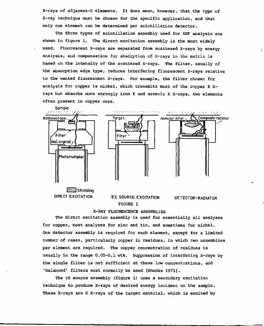
X-rays of adjacent-Z elements. It does mean, however, that the type of
X-ray technique must be chosen for the specific application, and that
only one element can be determined per scintillation detector.
The three types of scintillation assembly used for XRF analysis are
shown in figure 1. The direct excitation assembly is the most widely
used. Fluorescent X-rays are separated from scattered X-rays by energy
analysis, aud compensation for abso'rption of X-rays in the matrix is
based on the intensity of the scattered X-rays. The filter, usually of
the absorption edge type, reduces interfering fluorescent X-rays relative
to the wanted fluorescent X-rays. For example, the filter chosen for
analysis for copper is nickel, which transmits most of the copper K X-
rays but absorbs more strongly iron K and arsenic K X-rays, two elements
often present in copper ores.
Sample
Radioisotope Composite radiator
Photomultiplier
DETECTOR-RADIATOR
W/A Shielding
DIRECT EXCITATION &X SOURCE EXCITATION
FIGURE 1
X-RAY FLUORESCENCE ASSEMBLIESThe direct excitation assembly is used for essentially all analyses
for copper, most analyses for zinc and tin, and sometimes for nickel.
One detector assembly is required for each element, except for a limited
number of cases, particularly copper in residues, in which two assemblies
per element are required. The copper concentration of residues is
usually in the range 0.05-0.1 wt%. Suppression of interfering X-rays by
the single filter is not sufficient at these low concentrations, and
'balanced1 filters must normally be used [Rhodes 1971].
The yX source assembly (figure 1) uses a secondary excitation
technique to produce X-rays of desired energy incident on the sample.
These X-rays are K X-rays of the target material, which is excited by

182
Y-rays from the radioisotope source. Hence the atomic number of the
target material determines the energy of the incident X-rays. The
yX source assembly has been mainly used to determine tin at very low
concentration in residue streams. The main limitation to sensitivity in
this case is due to scattered X-rays whose intensity increases rapidly
with increase of incident X-ray energy. Sensitivity is much improved in
this case by selecting the energy to be just above the K shell absorption
edge of tin.
The detector-radiator assembly (figure 1) has excellent discrimination
(e.g. by a factor of 25) against interfering X-rays of energy less than
that of the fluorescent X-rays of the wanted element [Watt 1972]. The
basis of its discrimination is that the radiator element can be chosen
so that only the higher of the two close-in-energy X-ray components has
sufficient energy to excite K X-rays of the radiator element. The
detector is shielded from the sample and hence 'sees' only X-rays emitted
by the radiator. The intensity of higher energy X-rays scattered from
the sample can also be measured simultaneously in the one assembly by
use of a second radiator element of atomic number considerably higher
than that of the first radiator. The spectrum is similar in shape to
that in figure 2. This assembly gives very good sensitivity when deter- '
mining nickel in iron-rich ores and lead in zinc concentrates, zinc in
copper concentrates, etc.- It is only used in those cases in which
insufficient sensitivity is obtained using the direct excitation assembly.
10
aj 4
01bockscottered
X-roys
5 10 !5 20ENERGY (keVJ
FIGURE 2
TYPICAL SPECTRUM OF X-RAYS FROM ACOPPER ORE SLURRY EXCITED BYX-RAYS FROM 238Pu AND MEASUREDUSING A SCINTILLATION DETECTOR
25

183
2.3.2 X-ray preferential absorption (XRA) analysis
This technique is based on the collimated beam absorption of X-rays
of energy greater than that of the K shell absorption edge of the
wanted element. Since the wanted element usually has an atomic number
much higher than that of other elements in the matrix, it absorbs a much
greater proportion of X-rays per unit weight than does the matrix. In
practice, this means that, at high concentrations of the wanted element,
a measurement at one X-ray energy compensated for changes in slurry
solids content by a high energy Y~ray absorption measurement is sufficient
to determine the concentration of the wanted element. For example, lead
in flotation feeds at the Broken Hill concentrators can be determined by
measurements of 100 keV absorption (153Gd), and 662 keV absorption
(137Cs) for slurry solids content [Ellis et. al. 1969]. At low concentrations
of wanted element, where the matrix absorbs a significant proportion of
X-rays, a second X-ray measurement must be made at.an energy below that
of the absorption edge of the wanted element.
2.3.3 Advantages of scintillation detector systems
The main advantageQ in the use of scintillation detectors in on-
stream analysis systems are:
(a) techniques are simple;
(b) equipment is robust and long-proved in industrial use;
(c) detectors can be contained in probes immersed in the process
stream (hence avoiding the need for sample by-lines).
2.4 Proportional Detectors
The techniques used with high resolution proportional detectors
have been described in Part B of this series. The main advantage of
using proportional detectors is that simultaneous analysis for a maximum
of about four elements can be made with the one head unit. Sensitivity
and accuracy are about the same as for scintillation detectors. The
electronics used with proportional detectors is relatively complex, and
frequent checks of stability must be made with reference samples.

184
3. BIBLIOGRAPHY
Basinger, T.F. [1973] - Process Control X-ray Quantometer for High
Precision Slurry Stream Analyses. Tree.Synp.Review of On-Stream
Analysis Practice, Kalgoorlie. Australian Mineral Industries
Research Association Ltd., Melbourne, p. 35.
Ellis, W.K., Fookes, R.A., Gravitis, V.L. & Watt, J.S. [1969] - Radioisotope
X-ray Techniques for On-stream Analysis of Slurries. Feasibility
studies using Solid Samples of Mineral Products. Int.J.Appl.Radiat.
Isot., 20;691.
International Atomic Energy Agency [1970] - Radioisotope X-ray Fluorescence
Spectrometry. Report on Panel Meeting, Vienna, 1968. IAEA Technical
Report Series No.115, IAWA, Vienna.
Leskinen, T., Koskinen, J., Lappalainen, S., Niitti, T. & Vanninen, P.
[1973] - Performance of On-stream Analysers at Outokumpu Concentrators,
Finland. CIM (Can.Min.Metall.Bull), 66(730)37.
Rhodes, J.R. [1971] - Design and Application of X-ray Emission Analysis
using Radioisotope X-ray or Y~ray Sources. ASTM Special Publication
485, American Society for Testing and Materials, pp. 243-284.
Watt, J.S. [1972] - Radioisotope Detector-Radiator Assemblies in X-ray
Fluorescence Analysis for Copper and Zinc in Iron-rich Minerals.
Int.J.Appl.Radiat.Isot., 23;257.
Watt, J.S. [1977] - Nuclear Techniques for On-line Measurement in the
Control of Mineral Processing. In Nuclear Techniques and Mineral
Resources 1977. IAEA, Vienna, pp. 569-602.
Watt, J.S. & Gravitis, V.L. [1973] - Radioisotope X-ray Fluorescence
Techniques applied to On-stream Analysis of Mineral Process
Streams. IFAC Symposium on Automatic Control in Mining Mineral and
Metal Processing. Institution of Engineers, Australia, National
Conference Publication No. 73/4, p.199.

185
PART D
ON-STREAM ANALYSIS SYSTEMS
by
W.J. Howarth
J.S. Watt
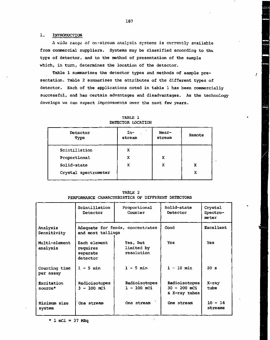
187
1. INTRODUCTION
A vd.de range of on-strcair. analysis systems is currently available
from commercial suppliers. Systems may be classified according to tht
type of detector, and to the method of presentation of the sample
which, in turn, determines the location of the detector.
Table 1 summarises the detector types and methods of sample pre-
sentation. Table 2 summarises the attributes of the different types of
detector. Each of the applications noted in table 1 has been commercially
successful, and has certain advantages and disadvantages. As the technology
develops we can expect improvements over the next few years.
TABLE 1DETECTOR LOCATION
DetectorType
Scintillation
Proportional
Solid-state
Crystal spectrometer
In-stream
X
X
X
Near-stream
X
X
Remote
X
X
TABLE 2PERFORMANCE CHARACTERISTICS OF DIFFERENT DETECTORS
AnalysisSensitivity
Multi-elementanalysis
Counting timeper assay
Excitationsource*
Minimum sizesystem
ScintillationDetector
ProportionalCounter
Adequate for feeds, concentratesand most tailings
Each elementrequiresseparatedetector
1 - 5 min
Radioisotopes3 - 100 mci
One stream
Yes, butlimited byresolution
1 - 5 min
Radioisotopes1 - 100 mCi
One stream
Solid-stateDetector
Good
Yes
1-10 min
Radioisotopes30 - 200 mCi& X-ray tubes
One stream
CrystalSpectro-meter
Excellent
Yes
20 s
X-raytube
10 - 14streams
* 1 mCi = 37 MBq

188
2. X-RAY TUBE/CRYSTAL SPECTROMETER SYSTEMS
The current versions of this type of system [Leskinen et al. 1973,
Basinger 1973] were developed over at least twenty years with many
notable failures along the way. Essentially, they follow the conventional
approach of piping slurry samples into a laboratory-type XRF analyser.
These systems sequentially analyse slurries sampled from up to 14
process streams and routed to a central air-conditioned room housing the
crystal spectrometer. The 14 slurry by-lines are installed side-by-side
in the room, and each has a flow cell with a thin window. The crystal
spectrometer automatically moves to the position in front of each flow
cell window, is stationary for 20 seconds while the analysis is made,
and then moves to the next window.
PROCESSFLOW
SECONDARYSAMPLE
SAMPLECELL FLOW5 GPM
TIMEDSAMPLE
FIGURE 1
A SAMPLING CIRCUIT OF THE "COURIER-300" SYSTEM
A typical sampling system is shown in figure 1. A primary sample
of about 200 L min 1 is continuously taken from the process stream by an
appropriate saiup.ler. The continuous samples are routed to the central
laboratory, where each -by-line is cut by a secondary sampler (figure 2)
to 20 L min"1 which passes through the individual flow cells for analysis.
The slurry overflows are returned to the process streams.
Several elements can be determined simultaneously by using several
scintillation detectors with the fixed crystal spectrometer. This, and
the capability to analyse up to 14 streams with one crystal spectrometer,
are the main advantages of the system.

189
The overall system, involving two-stage sampling, long routing of
slurries about the concentrator, flow cells, and the precise positioning
required for the spectrometer, is complex and very expensive. Sampling
systems are critical and require much maintenance (compared with immersion
probe and short by-line systems). The developments in these systems
over the past 20 years have led to reliable on-stream analysis, and the
largest number of commercial on-stream analysis systems are of this
type.
Two manufacturers are prominent in this field, namely, Applied
Radiation Laboratories (ARL) in the USA, and Outokumpu Oy in Finland.
The main advanbaqos of these systems are their ability to analyse
several elements simultaneously, and a good sensitivity which enables
low levels of metal concentration to be determined. The disadvantages
are high cost, inflexibility and uncertain reliability owing to the
complexity of equipment plus the problems of pumping samples through
small diameter lines.
3. SCINTILLATION DETECTOR SYSTEM
Scintillation detectors form the basis of immersion probes for in-
stream systems [Watt & Gravitis 1973, Watt 1977]. These systems, supplied
by the Australian Mineral Development Laboratories (AMDEL), are based on
research and development by the Australian Atomic Energy Commission.
The X-ray techniques are discussed in Part C of this series.
•vT
' FIGURE 2
CUTTER TYPE SECONDARY SAMPLINGSYSTEM AT THE PYHASALMI CONCENTRATOR

VDO
FIGURE 3
RADIOISOTOPE IMMERSION PROBES

191
Immersion probes for in-stream use are shown in figure 3. Each
contains a radioisotope source and a scintillation detector. The probes
feed signals to an electronic unit located nearby. A small digital
computer in the plant control room receives output from a number of
these units and then calculates the concentrations of wanted elements in
the various streams in which the probes are immersed. The general
configuration is shown in figure 4.
Teletype or VisualDisplay Unit
FIGURE 4
GENERAL CONFIGURATION OF ANIMMERSION PROBE SYSTEM
The XRF probes have outer windows of Mylar or Kaptan, normally of
thickness 0.05 mm. These windows are usually changed every two to
twelve months, the frequency depending on the abrasiveness of the slurry.
There is also an inner window in each probe; a sensor detects ingress of
slurry past the first or both windows, and activates an alarm in the
plant control room to signal window rupture.
A typical 'analysis' zone into which the probes are immersed is
shown in figure 5. To minimise air entrainment in the analysis zone,
slurry is entered below the surface of the slurry in the zone; in
addition, one or two baffle plates are installed. A small agitator ensures
that the turbulence in the zone is sufficient to provide good mixing.
The uniformity of slurry throughout the analysis zone is checked at the
time of installation by using a density probe to measure slurry density
throughout the zone.

192
FIGURE 5
A TYPICAL ANALYSIS ZONE FOR A15 TONNE PER HOUR TIN FLOTATION
STREAMEach scintillation detector probe is designed to analyse for one
element only, so when several elements have to be analysed, or when
inter-element corrections are required, several probes are needed.
A typical installation to measure copper and zinc would require
a copper probe, a zinc probe, and a slurry density probe. Note that a
slurry density probe is required to correct for variations in solids
content of the slurry.
Accuracies obtainable with scintillation detector immersion probes are
Feeds 5 - 8 \
Concentrates 1 - 5 \ % relative
Tailings 8 - 12 )
The minimum detectable level is about 0.01 wt% of the metal being
analysed by this type of detector. Therefore, for very low value
tailings, as in copper operations where the copper level may be 0.05 wt%,
scintillation detectors do not give sufficient sensitivity. In these
circumstances, it is necessary to use a solid-state detector probe.
The advantages of scintillation detector systems are low cost, ease
of maintenance and operation, and reliability. The immersion probe
concept is also very flexible. The only major disadvantages are the
lack of sensitivity to low levels of metal and the need to increase the
number of probes to handle multiple elements or inter-element corrections.

193
4. PROPORTIONAL DETECTOR SYSTEM
An on-stream analysis system based on an in-stream probe containing
a high resolution proportional detector is shown in figure 6 [Hietala &
Viitanen 1978].
•/C'TAsrREGULATORSDISCRIMINATORSPULSE REGISTERSCONTROL LOGICSCOMMUNICATION
ROTATINGMECHANISM —
^
^ ^>,
t t t111 .1 •
11
, I,~^n fs—_B B_
PULSE SHAPING
FIGURE 6
PROBE FOR ON STREAM ANALYSIS OFMINERAL SLURRIES AND INCORPORATINGA RADIOISOTOPE X-RAY SOURCE AND A
HIGH RESOLUTION PROPORTIONAL DETECTOR
The overall performance of the detector, electronics, and spectrum
stripping techniques is checked regularly by the system's computer using
measurements of reference samples which are automatically rotated before
the detector. The probe can be used in-stream but it is recommended by
the manufacturer (Outokumpu Oy, Finland) that it be used on a sample by-
line with a flow ce!2. dimensioned for flow rates in the range 150-250
L min 1. This flow cell can be fed directly from the primary sampler
without the need for pumping. The accuracies expected under normal
operating conditions are:
Analysis Range
(wt %)
0.1-0.5
0.5-5
>5
Relatives Accuracy
(%)
5-15
3-8
1-5

194
The minimum detectable level is about 0.01 wt%. This type of probe was
installed at the Keretti concentrator, Finland, in June 1976 to analyse
for the elements copper, zinc, cobalt, nickel and iron in two streams,
zinc rougher concentrate and feed of the zinc rougher circuit.
The system does not seem to have been widely accepted by the
mineral industry and there is very little information available on long-
term accuracy and maintenance requirements. A trial in Canada on a
copper zinc ore is known to have resulted in satisfactory accuracy on
feeds and concentrates but unsatisfactory results on tailings. Sub-
sequently, a solid-state detector was installed in the tailings stream.
5. SOLID-STATE DETECTOR SYSTEMS
Solid-state detectors have only recently come into prominence, with
four manufacturers now offering on-stream analysis systems based on.
these detectors. Systems are available either as a near-stream option
or in an immersion probe configuration for in-stream use.
5.1 Near-stream System
The near-stream systems [Watt 1977] allow two to four streams to be
analysed by one detector. Figure 7 shows a typical sampling system.
The sample by-line arrangement of an on-stream analysis system is based
on a solid-state detector, a radioisotope source and a short sample by-
line.
OVERFLOW RETURNEDTO PUMP BOX
^-SCREEN (6mm MESH)
SECONDARYSAMPLt
SPIGOT OR SAMPLETHIEF ON PUMPDISCHARGE
RETURNED TOPUMP BOX
PRIMARYSAMPLE
SECONDARY SAMPLE FROMANOTHER STREAM
•CABINET
SLURRY SWITCHINGMECHANISM
BYPASS PIPE
SOLID-STATE DETECTOR
FIGURE 7
A SAMPLING SYSTEM USED IN AN ON-STREAM ANALYSERBASED ON A SOLID-STATE DETECTOR LOCATED IN THE
THE PLANT CLOSE TO A PROCESS

195
The primary sample, taken from the process stream of vertically rising
slurry, flows into the primary sample tank in which the slurry is de-
aerated and screened for foreign objects. A secondary sample of much
smaller flow rate is taken from this tank through a device which allows
slurries from up to four separate by-lines to be routed through the
sample flow cell viewed by the solid-state detector. The detector and
associated electronics are enclosed in a temperature-controlled cabinet
which is mounted near the process streams, so avoiding the settling
problems associated with long runs of pipe. This on-stream analysis
system has been tested in plant trials at Noranda Mines Ltd, Ontario,
Canada for copper, lead and zinc and is now installed in three mineral
concentrators in Canada. This system is manufactured by Inax Instruments
Lt.d, and Bondar & Clegg of Canada.
Counting time for low metal values can be long to achieve the best
precision, since there may be only a few counts per second in a particular
channel. Although it is generally considered desirable to limit counting
times to five minutes, up to ten minutes may be necessary for levels
below 0.1 per cent. This means possibly excessive times between reporting
assays if more than two streams are to be analysed by the same detector.
5.2 In-stream System
An in-stream probe system [Watt 1977] is manufactured by the Nuclear
Equipment Corporation, USA, and AMDEL has a licensing agreement to
market the probes. The in-stream probe is illustrated in figure 8.
This type of probe would generally be used only in tailing streams or
where several elements need to be assayed simultaneously. .
INSCANSolid StateDetectorProbe ...
Line Receiver Mini or MicroComputer
Signal Analyser 2
FIGURE 8
SOLID-STATE DETECTOR IN-STREAM PROBE
Teletype or VisualDisplay Unit

196
The solid-state detector resolutions obtained under plant conditions
will generally be of the order of 200-300 eV. Minimum detectable
levels for most elements will be around 0.005 per cent, allowing sufficient
analytical accuracy for the vast majority of applications.
The disadvantages of solid-state detectors are cost, sensitivity to
vibration and electrical interference, and the necessity to maintain a
supply of liquid nitrogen (2-4 litres per week per detector).
6. GENERAL REQUIREMENTS
On-stream analysis systems represent relatively complex technology
operating in a harsh environment, mostly with rather poor maintenance
facilities and a long way from major centres of industry. A successful
system will have been designed to withstand the harsh environment and to
be maintained at the first level by process personnel rather than instrument
technicians. Therefore, the system should be as simple as possible,
robust and of modular design so that faults can be easily identified and
rectified by replacement of modules rather than components.
Availabilities of over 95 per cent are possible from the successful
systems currently available. This high availability is essential because
poor system performance, even for a short time, may result in loss of
operator confidence and long-term rejection of the system as an operating
tool.
Speed of response is important.. In general, each assay should be
available at least once every 15 minutes. Shorter times may be desirable
in some situtations where the system is used as the basis of process
control.
Very approximate numbers of commercial- systems in current use are
as follows:
X-ray tube systems : Applied Radiation Laboratories 29
: Outokumpu Oy (Courier system) 22
Scintillation detector systems : AMDEL 16
Solid-state detector systems : Inax, and Bondar & Clegg 4
Proportional counter systems : Outokumpu Oy 2
The authors believe that the future direction will be towards
smaller systems which offer the advantage of lower cost, more flexibility .
and simpler installation and maintenence requirements.
197
7. BIBLIOGRAPHY
Basinger, T.F. [1973] - Process Control X-ray Quantometer for High
Precision Slurry Stream Analyses. Proc.Symp. Review of On-Stream
Analysis Practice, Kalgoorlie. Australian Mineral Industries
Research Association Ltd., Melbourne, p. 35.
Hietala, M. & Viitanen, J. [1978] - A Radioisotope On-stream Analyser
for the Mining Industry. In Advances in X-ray Analysis (eds.
Barrett, C.S., Leydon, D.W., Newkirk, J.B., Rudd, C.O.) Vol. 21,
Plenum Press, New York, pp. 193-205.
Leskinen, T., Koskinen, J., Lappalainen, S., Niitti, T. & Vanninen, P.
[1973] - Performance of On-stream Analysers at Outokumpu Concentrators,
Finland CIM (Can.Min.Metall.Bull.), 66(730)37.
Watt, J.S. & Gravitis, V.L. [1973] - Radioisotope X-ray Fluorescence
Techniques Applied to On-stream Analysis of Mineral Process Streams.
IFAC Symposium on Automatic Control in Mining, Mineral and Metal
Processing. Institution of Engineers, Australia, National Conference
Publication No. 73/4, p 199.
Watt, J.S. [1977] - Nuclear Techniques for On-line Measurement in
Control of Mineral Processing. Proc.Symp. Nuclear Techniques and
Mineral Resources, IAEA, Vienna, pp.569-602.

199
PART E
APPLICATIONS OF ON-STREAM ANALYSIS SYSTEMS
by
W.J. Howarth
201
1. BENEFITS OF ON-STREAM ANALYSIS
1.1 Types of Benefit
On-stream analysis permits closer control of the metallurgical
process, and brings increased efficiency and economic benefit through :
li) increased mineral recovery;
(ii) improved or more stable concentrate grade;
(iii) reduced consumption of reagents;
(iv) reduction in labour requirements for sampling and analysis;
and
(v) greater efficiency of experimentation and innovations.
Naturally, the particular benefits change from place to place, a«d are
not always evident or recorded in each plant, but all of those benefits
noted above have been experienced in Australian concentrators using
immersion probes and have been reported in the world literature.
The economic justification for purchasing and installing an on-
stream analysis system derives from an expected increase in efficiency
of operation. The simplest criterion is based on the concept of pay-
back time, i.e. the time over which the increased income from on-stream
analysis returns the installed cost of the system.
The following sections detail benefits of on-stream analysis as
given in published reports, or from direct communication with plant
operators.
1.2 Increased Metal Recovery
Concentrators normally operate in the recovery range 85-95 per
cent. Because of the large tonnage rates processed, small increases in
recovery can bring large increases in the value of concentrate. Some of
the examples in table 1 include automatic control.
In summary, increases in metal recovery from 0.1-3.0 per cent have
been reported by users of on-stream analysis who have kept careful
records. There has been no published record of a user who has made a
careful study and reported no improvement. Many users have reported
that they believe there has been an improvement, but cannot prove the
result owing to inadequate records or other complicating factors such as
change in circuit or change in ore grade.
1.3 Reduced Consumption of Reagents
Flotation reagents are an important component of the cost of pro-
cessing ore. Recent advice from reagent suppliers shows that reagent
costs are approximately as outlined in table 2.

202
- TABLE 1
REPORTED INCREASES IN METALLURGICAL RECOVERY
Users
. E.Z. Co (Australasia) )
. North Broken Hill Ltd |
. Zinc Corporation )
. Mt Isa Mines
. Lake Dufault i
. Ecstall Concentrator V
. Mattagami Lake Mines /
Outokumpu Oy ConcentratorsVihantiKerettiPyhasalmiKotalahti
System
AMDEL
Courier
ARL
Courier
% Increase
0.73.0
small improvement inrecovery
0.1
1-20.81.61.0
2.50.32.01.0
Element
ZnZnZn
Cu
CuCuZnCu
CuCuCuCu
TABLE 2
REAGENT COSTS($US/tonne of ore processed)
Ore Type
Pb/Zn(difficult ore)
Pb/Zn (simple ore)V. large porphyry
Cu
Average Cu
Ni
Collector
0.34
0.075
0.12
0.15
0.43
Frother
0.07
0,024
0.035
-0.005
Activator
0.11
0.16
-0.04
Depressant
0.26
0.018
-
0.035
Other
0.025
0.03
0.095
-
-
Total
0.805
0.304
0.142
-
0.825
Users of on~stream analysis have published the following data on
reduction in use of reagents :
Zinc Corporation Ltd Pb/Zn
Mt Isa Mines Cu
Strathcona Ni
Mattagami Lake Mines Zn/Cu
% in collector
6.6 cents/tonne ore
Outokumpu Oy Concentrators report approx. 20% in reagent
In general, reductions from 10-40 per cent in various reagents have been
reported.

203
1.4 Increases in Concentrate Grade
Increases in concentrate grade return economic benefits in the form of
reduced smelter charges, and
reduced costs of transportation of concentrate.
Increases in concentrate grade, or more precise control of concentrate
at a specified grade, have been reported by many users and are listed ir.
table 3.
TABLE 3
PERCENTAGE INCREASES IN CONCENTRATE GRADE
User Element % Increase
Mt Lyell Mining & Railway Co
North Broken Hill
Western Mining Corporation
Strathcona (Falconbridge)
E.Z. Co (Australasia)
Kidd-Creek (Ecstall)
Mattagami Lake Mines
Cu
Pb
Ni
Ni
Zn
CuZn
Zn
1
3
more stable
20 (reduction in gangue)
more stable
0.630.88
0.4
It is difficult to calculate the exact economic gain in most cases,
as transport costs and smolter contracts are not known. However tho
benefits, where calculated, have been large although not as large as
those from increased metal recovery and reduction in the use of reagents.
1.5 Savings in Labour
In Australian mines, the cost, of labour is high because the actual
wages paid to a worker are only a part of the cost. Other factors are :
allowance for sick leave and long service leave,
contribution to superannuation,
over-award payments for remote locations,
. payroll tax,
allowances for housing, and
; relocation costs.
• The total cost per employee in remote locations can be very high.
In the new uranium provinces in Australia's north, the cost of one
additional worker is approximately $80 000 in the first year*. Even in
thfe more established areas, the cost will not be less than $25 000 per
year.
* Costs are based on the 1980 Australian dollar.

204
Most on-stream analysis users report a reduction in the number of
samplers, depending on the size of concentrator and the extent of sam-
pling. In the normal concentrator, it is expected that there would be
at least one person on each shift collecting and processing regular
samples, and additional personnel on day shift. The shift samplers can
conveniently be excluded, but it is usual to retain the day shift sam-
plers, possibly with an extra person to supervise the on-stream analysis
system. The net reduction would be two people.
1.6 Summary of Typical Benefits
Increases in recovery 0.1-3 per cent
Reduction in reagents 10-40 per cent
Concentrate grade increases 0.5-1 per cent
Reduction in workers up to seven in one case.
To translate these benefits into monetary values, it is necessary to
introduce the specific details of a particular concentrator :
metal processed,
annual tonnage,
head grade, and
ex-mine value of concentrate.
Each case is different and the detailed calculations are not justified
here. The kind of payback time normally found is one year or less.
Paybacks as short as three months have been reported.
2. ANALYSIS ZONES FOR IMMERSION PROBES
2.1 Requirements
One of the critical factors in obtaining a successful plant instal-
lation of immersion probes for on-stream analysis is the provision of
suitable analysis zones. An analysis zone is defined as the volume of
pulp into which the probes are immersed.
The design of the analysis zone must be such that the sample of
pulp 'seen' by the probes is representative of the total volume of pulp
passing the probes (i.e. representative of the total stream) and is not
subject to excessive or variable aeration. An ideal analysis zone is
perfectly mixed and free from air. A poorly designed analysis zone can
give rise to incorrect assays as a result of (a) segregation, or (b)
excessive or variable aeration.
2.2 Segregation
Segregation results if the flow pattern in the analysis zone does
not provide flow velocities sufficient to overcome the settling veloc-
ities of the heaviest and largest particles. The flow pattern of the

205
pulp is determined by two energy sources; one is the kinetic energy
(flow energy) of the pulp and the other is an external source such as an
agitator.
The flow energy of the pulp will generally not provide sufficient
mixing under normal process conditions because of the following factors :
variable flow-rate;
variable particle size distribution;
variable pulp density; and
variable mineral distribution.
Consequently, to prevent segregation problems, external agitation is
required to remove any doubts about the degree of mixing in the analysis
zone. The agitation should generally be provided by impellers with the
speed of rotation in the range 350 to 750 rev min"1, and with the diameter
designed to prevent segregation. The type of impeller can be varied to
suit the application, but would generally be either the propeller or the
flat blade turbine type. The mixing should not be so turbulent that it
causes air entrainment.
2.3 Aeration
The probes effectively measure the weight of a particular element
per unit volume of pulp, yet are calibrated in terms of weight of ele-
ment per unit mass of dry solids (i.e. dry solids assay). For a given
dry solids assay, the weight of the element per unit volume of pulp
depends on both pulp density and aeration.
The density probe corrects for changes in pulp density, but cannot
distinguish between a change in pulp density and a change in aeration.
A relatively small degree of aeration can be tolerated, provided that it
does not vary greatly. Excessive aeration, even if constant, reduces
the sensitivity of the probe.
The effect of aeration is most severe when the wanted element is
determined by gamma-ray absorption techniques (e.g. Pb, W, Bi) and less
of a problem when XRF methods are used (as for Fe, Ni, Cu, Zn, Sn, etc).
General experience has shown that minor aeration can be tolerated with
most fluorescence probe installations.
Aeration can be minimised by the correct design and location of the
analysis zone. For instance, probes should not be located in flotation
bank feed or tailing boxes, or in flotation conditioning tanks where
aeration is encouraged.
2.4 Design of Analysis Zones
As is shown in figure 1, a typical analysis zone contains four
major sections :
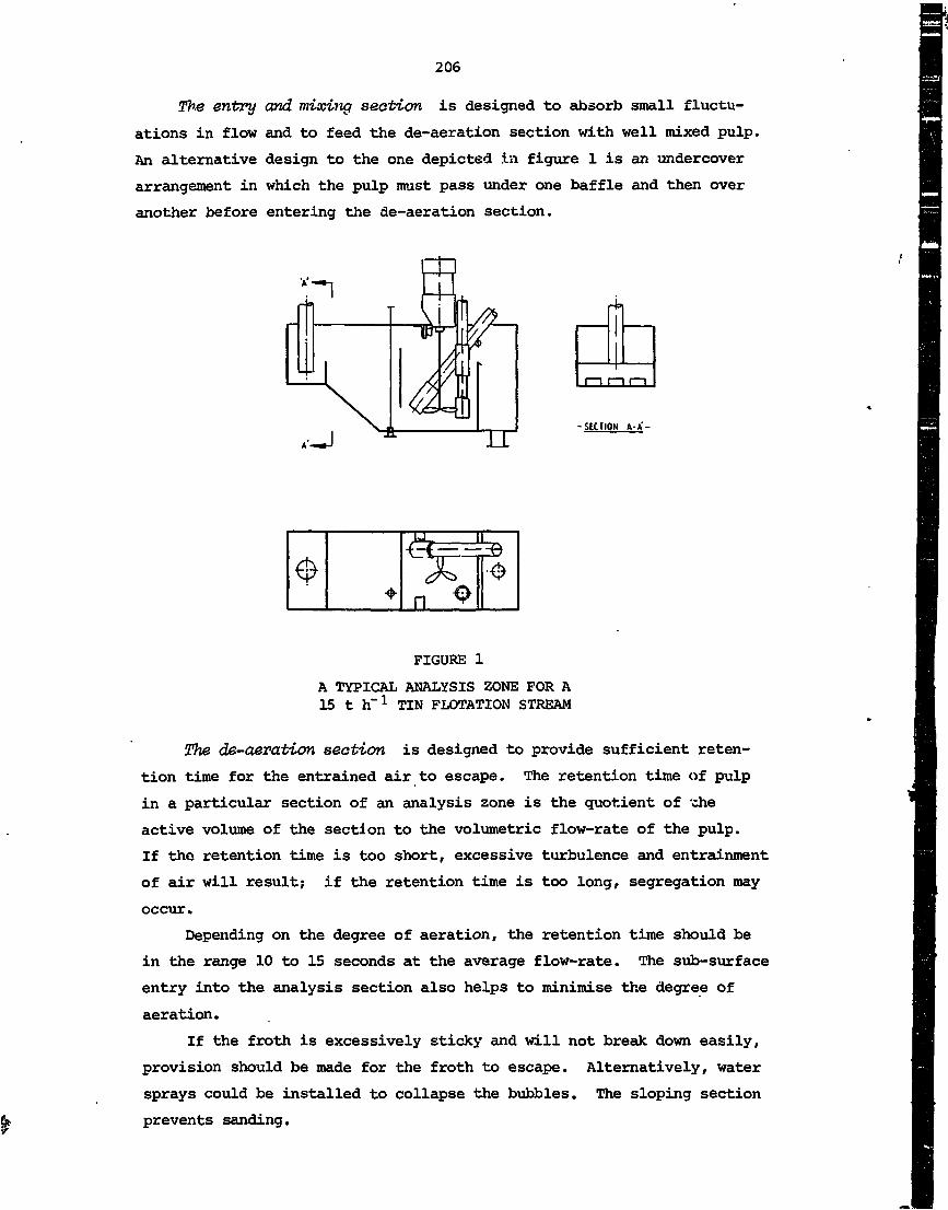
206
entry and missing section is designed to absorb small fluctu-
ations in flow and to feed the de-aeration section with well mixed pulp.
An alternative design to the one depicted in figure 1 is an undercover
arrangement in which the pulp must pass under one baffle and then over
another before entering the de-aeration section.
-SECTION A-A'-
M,
n
FIGURE 1
A TYPICAL ANALYSIS ZONE FOR A15 t h"1 TIN FLOTATION STREAM
The de-aeration section is designed to provide sufficient reten-
tion time for the entrained air to escape. The retention time of pulp
in a particular section of an analysis zone is the quotient of -che
active volume of the section to the volumetric flow-rate of the pulp.
If tho retention time is too short, excessive turbulence and entrainment
of air will result; if the retention time is too long, segregation may
occur.
Depending on the degree of aeration, the retention time should be
in the range 10 to 15 seconds at the average flow-rate. The sub-surface
entry into the analysis section also helps to minimise the degree of
aeration.
If the froth is excessively sticky and will not break down easily,
provision should be made for the froth to escape. Alternatively, water
sprays could be installed to collapse the bubbles. The sloping section
prevents sanding.

207
The analysis section houses the immersion probes and the stirrer,
and is designed to produce an average retention time in the section of
10 to 15 seconds. The height of the inlet into the analysis section
should be chosen to give a pulp velocity of 0.3 to 0.5 m s~1 so that
sanding at the base of the de-aeration section does not occur.
The design velocity can be varied according to the pulp character-
istics, e.g. particle size, specific gravity of the solids, etc. A
manually adjustable gate in this position has often been useful when
plant throughputs vary markedly in the long term. Some applications
require a sand gate at the base of the overflow weir to assist the
removal of coarse particles.
The discharge section collects the pulp discharging from the
analysis section and an attached pipe transports the pulp to the next
stage in the process. This section need not be very large but it should
be large enough for a sample cutter to be easily moved along the over-
flow weir. This is a convenient point for collecting a representative
sample of the pulp stream.
The above description applies to the normal analysis zone design. •
In some circumstances modifications are necessary. For example in
applications where the pulp flow-rates are high, it is generally neces-
sary to reduce the recommended retention times so that the analysis zone
is a practical size. In applications where the pulp flow-rates are
extremely low, it is necessary to design the minimum size analysis zone
that will house the probes and the stirrer, even though the retention
times may well exceed the recommended figures.
Analysis zones can usually be located within the process such that
additional pumps are not necessary. Typical locations include above-
pump sumps, above-flotation feed boxes, above-mixing or conditioning
tanks, etc. In these locations, the pipes that feed the above-mentioned
process units are simply directed to the analysis zone, with the dis-
charge gravitating to the process unit below. In some cases, it may be
possible to modify existing process units, e.g. mixing tanks, launders,
etc., by incorporating baffles and a stirrer.
The following are general recommendations on the design and loca-
tion of analysis zones :
(a) The zone should be constructed from 4 mm mild steel plate with
6 mm thick soft rubber lining.
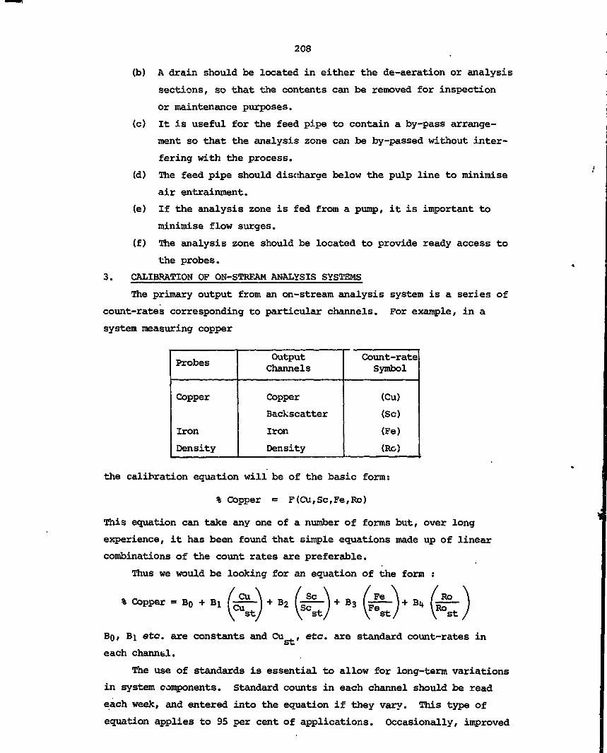
208
3.
(b) A drain should be located in either the de-aeration or analysis
sections, so that the contents can be removed for inspection
or maintenance purposes.
(c) It is useful for the feed pipe to contain a by-pass arrange-
ment so that the analysis zone can be by-passed without inter-
fering with the process.
(d) The feed pipe should discharge below the pulp line to minimise
air entrainment.
(e) If the analysis zone is fed from a pump, it is important to
minimise flow surges.
(f) The analysis zone should be located to provide ready access to
the probes.
CALIBRATION OF ON-STREAM ANALYSIS SYSTEMS
The primary output from an on-stream analysis system is a series of
count-rates corresponding to particular channels. For example, in a
system measuring copper
Probes
Copper
Iron
Density
OutputChannels
Copper
Backscatter
Iron
Density
Count-rateSymbol
(Cu)
(Sc)
(Fe)
(Ro)
the calibration equation will be of the basic form:
% Copper = F(Cu,Sc,Fe,Ro)
This equation can take any one of a number of forms but, over long
experience, it has been found that simple equations made up of linear
combinations of the count rates are preferable.
Thus we would be looking for an equation of the form :
% Copper = BQ + + B3
BQ, BI etc. are constants and Cu , etc. are standard count-rates inS*C
each channel.
The use of standards is essential to allow for long-term variations
in system components. Standard counts in each channel should be read
each week, and entered into the equation if they vary. This type of
equation applies to 95 per cent of applications. Occasionally, improved

209
accuracy can be obtained by incorporating a logarithmic or squared term.
This is mainly where the range of metal assays may be very large.
To calibrate a system, count-rates are recorded while a sample is
being taken, being careful to synchronise the two events. The sample is
assayed and sample assays correlated against the count-rates by multiple
linear regression analysis, which uses least squares method to optimise
the constants BQ, Bj, etc. to obtain the best fit between assays and
count-rates.
It is important to take the results over a sufficient period to
cover the full range of all the variables, and at least 20 samples
should be taken.
4. CARE AND MAINTENANCE OF AN ON-STREAM ANALYSIS SYSTEM
The full potential benefit from an on-stream analysis system can
only be realised if the system is maintained at a high level of opera-
tional performance; as with any system, a certain minimum level of care
and maintenance must be maintained.
During the commissioning and immediate post-commissioning stages,
a normal three-stream immersion probe system can occupy most of the time
of a metallurgist, with the help of a laboratory technician. Once the
system is operating on a routine basis, regular attention is still
required, but at a reduced level. This routine maintenance can be
performed by a laboratory technician and should involve, on average,
approximately 30 minutes per stream per day. A metallurgist should
supervise calibration and trouble shooting.
An appropriate care and maintenance schedule is based on operating
experience and is designed to identify faults and maintain the cali-
bration accuracy of the probes. As with any analytical technique,
regular standardisation and maintenance is essential. It is also
important that a continuous record of standard count-rates, X-ray
spectra, assay calibration equations, component failures, etc. be kept.
In addition, a regular check on the performance of the system
should be undertaken by taking 8-hour (or 24-hour) composite samples
from the stream and assaying them by laboratory procedures. The 8-hour
average from the on-stream analysis system should be calculated and
compared against the sample assay. Any major discrepancy indicates that
investigation is necessary.

211
PART F
BENCH TOP AND PORTABLE MINERAL ANALYSERS, BOREHOLE
CORE ANALYSERS, AND IN SITU BOREHOLE LOGGING
by
W. J. Howarth
J. S. Watt
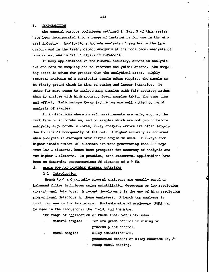
213
1. INTRODUCTION
The general purpose techniques out\ined in Part B of this series
have been incorporated into a range of instruments for use in the min-
eral industry. Applications include analysis of samples in the lab-
oratory and in the field, direct analysis at the rock face, analysis of
bore cores, and in situ analysis in boreholes.
In many applications in the mineral industry, errors in analysis
are due both to sampling and to inherent analytical errors. The sampl-
ing error is of'.en far greater than the analytical error. Highly
accurate analysis of a particular sample often requires the sample to
be finely ground which is time consuming and labour intensive. It
makes far more sense to analyse many samples with fair accuracy rather
than to analyse with high accuracy fewer samples taking the same time
and effort. Radioisotope X-ray techniques are well suited to rapid
analysis of samples.
In applications where in situ measurements are made, e.g. at the
rock face or in boreholes, and on samples which are not ground before
analysis, e.g. borehole cores, X-ray analysis errors are often largely
due to lack of homogeneity of the ore. A higher accuracy is achieved
when analysis is averaged over larger sample volumes. K X-rays from
higher atomic number (Z) elements are more penetrating than K X-rays
from low Z elements, hence best prospects for accuracy of analysis are
for higher Z elements. In practice, most successful applications have
been to determine concentrations of elements of Z > 50.
2. BENCH TOP AND PORTABLE MINERAL ANALYSERS
2.1 Introduction
'Bench top* and portable mineral analysers are usually based on
balanced filter techniques using scintillation detectors or low resolution
proportional detectors. A recent development is the use of high resolution
proportional detectors in these analysers. A bench top analyser is
.built for use in the laboratory. Portable mineral analysers (PMA) can
be used in the laboratory, the field, and the mine.
The range of application of these instruments.includes :
Mineral samples - for ore grade control in mining or
process plant control.
Metal samples - alloy identification,
- production control of alloy manufacture, or
- scrap metal sorting.
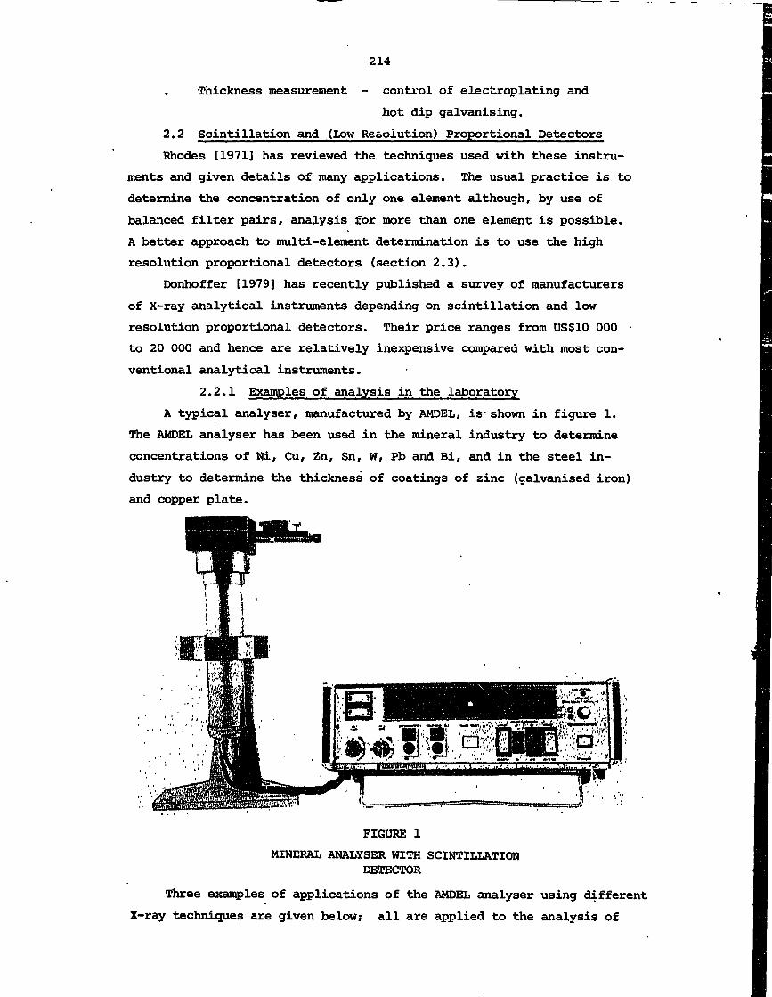
214
Thickness measurement - control of electroplating and
hot dip galvanising.
2.2 Scintillation and (Low Resolution) Proportional Detectors
Rhodes [1971] has reviewed the techniques used with these instru-
ments and given details of many applications. The usual practice is to
determine the concentration of only one element although, by use of
balanced filter pairs, analysis for more than one element is possible.
A better approach to multi-element determination is to use the high
resolution proportional detectors (section 2.3).
Donhoffer [1979] has recently published a survey of manufacturers
of X-ray analytical instruments depending on scintillation and low
resolution proportional detectors. Their price ranges from US$10 000 •
to 20 000 and hence are relatively inexpensive compared with most con-
ventional analytical instruments.
2.2.1 Examples of analysis in the laboratory
A typical analyser, manufactured by AMDEL, is- shown in figure 1.
The AMDEL analyser has been used in the mineral industry to determine
concentrations of Ni, Cu, Zn, Sn, W, Pb and Bi, and in the steel in-
dustry to determine the thickness of coatings of zinc (galvanised iron)
and copper plate.
FIGURE 1
MINERAL ANALYSER WITH SCINTILLATIONDETECTOR
Three examples of applications of the AMDEL analyser using different
X-ray techniques are given below; all are applied to the analysis of

215
samples from streams of mineral concentrators.
(a) Tin
Tin K X-rays are excited using 2t>1Am y-rays. The instrument
measures the intensities of X-rays in the tin K X-ray and backscattered
y-ray channels. In the absence of interfering elements, it is not
necessary to use balanced filters to obtain accurate analysis.
(b) Nickel
Nickel samples are accurately analysed using the detector-radiator
technique (see Part C of this series). Both nickel and iron K X-rays
are excited using X-rays from 238Pu, and the radiator suppresses the
iron K X-ray component. This technique can determine nickel in the
presence of high concentrations of iron, but is not successful when
cobalt or copper is present in appreciable quantities.
(c) Tungsten
Preferential X-ray absorption gives good accuracy of analysis for
tungsten if no lead is present. Separate measurements are made using
Y-rays from 153Gd (~100 keV) and 2tfiAm (60 keV) .
Note that in the above examples the ore was finely pulverised in
the grinding mills of the concentrator and no further preparation,
beyond drying the sample, was carried out. This is possible in many
cases where the 'natural grind1 is -150 ym.
2.2.2 Measurements at the rock face
The use of a portable mineral analyser to establish ore grades in a
mine by measurements in a channel cut across a rock face [Clayton, 1977]
is one example of the uses of a portable instrument. It enables a large
number of measurements to be carried out rapidly, and gives immediate
information to the mine management on the general changes in ore grade.
In practice, the number of chemical analyses required is greatly reduced
although regular calibration of the equipment is necessary.
Figure 2 shows a portable analyser being used to determine the
concentration of zinc across a rock face. Figure 3 shows the difference
count rates obtained across the face and also the assayed zinc content
determined chemically from chippings taken across the channel. It is
seen that relatively good correlation is achieved.
This technique for measuring at the rock face appears to be in only
limited use. The main disadvantage is that accuracy of analysis may be
very limited because of variations in grain size of the valuable mineral
and other components of the ore. Frequent calibration may be necessary,
hence many samples must be taken for the conventional assay required for
this calibration.

FIGURE 2
MEASUREMENT OF THE CONCENTRATIONOF ZINC ON THE ROCK FACE OF A MINE
USING A RADIOISOTOPE PORTABLE ANALYSER
0 o
100 200 300Distance along channel (cm)
FIGURE 3
COMPARISON OF ZINC CONTENT ACROSSA WORKING FACE DETERMINED BY
IN-SITU MEASUREMENT WITH A PORTABLERADIOISOTOPE ANALYSER AND ANALYSIS
OF A POWDERED CHANNEL SAMPLE
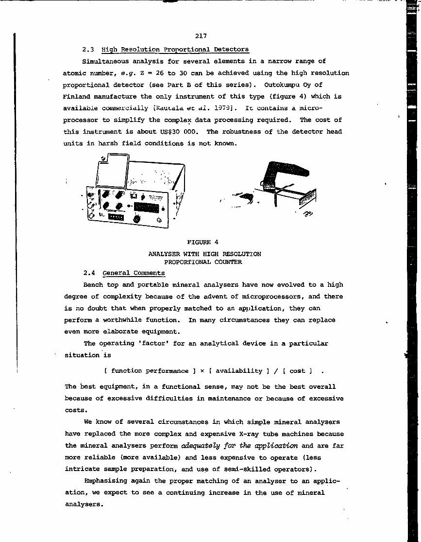
217
2.3 High Resolution Proportional Detectors
Simultaneous analysis for several elements in a narrow range of
atomic number, e.g. Z = 26 to 30 can be achieved using the high resolution
proportional detector (see Part B of this series). Outokumpu Oy of
Finland manufacture the only instrument of this type (figure 4) which is
available commercially [Raui-aid. ec ai. 1979] . It contains a micro-
processor to simplify the complex data processing required. The cost of
this instrument is about US$30 000. The robustness of the detector head
units in harsh field conditions is not known.
FIGURE 4
ANALYSER WITH HIGH RESOLUTIONPROPORTIONAL COUNTER
2.4 General Comments
Bench top and portable mineral analysers have now evolved to a high
degree of complexity because of the advent of microprocessors, and there
is no doubt that when properly matched to an application, they can
perform a worthwhile function. In many circumstances they can replace
even more elaborate equipment.
The operating 'factor1 for an analytical device in a particular
situation is
[ function performance ] x [ availability ] / [ cost ]
The best equipment, in a functional sense, may not be the best overall
because of excessive difficulties in maintenance or because of excessive
costs.
We know of several circumstances in which simple mineral analysers
have replaced the more complex and expensive X-ray tube machines because
the mineral analysers perform adequately foy the application and are far
more reliable (more available) and less expensive to operate (less
intricate sample preparation, and use of semi-skilled operators).
Emphasising again the proper matching of an analyser to an applic-
ation, we expect to see a continuing increase in the use of mineral
analysers.

218
3. MEASUREMENTS ON BOREHOLE CORES
An enormous number of cores are generally taken during exploration
and mine control operations. These are normally analysed by chemical
assay with significant time delays and at high cost. Equipment capable
of giving rapid «uialytical data has a strong appeal.
FIGURE 5
X-RAY FLUORESCENCE BOREHOLE COREANALYSER
Figure 5 shows a borehole core analyser developed to determine the
concentrations of tin [Clayton 1977]. in this equipment, characteristic
Sn K X-rays are excited by 241Am radioisotope sources, and detected on a
proportional counter incorporating balanced filters of palladium and
silver. The difference between the two readings is automatically indi-
cated. In addition, the intensity of scattered -y-rays is also measured
simultaneously and, by adjusting the measurement time so as to acquire a
constant number of scattered X-rays, the difference reading obtained is
directly proportional to tin concentration and independent of matrix
variations.
4. IN SITU BOREHOLE LOGGING
Borehole logging equipment based on XRF techniques is finding
increasing application in grade control. However, the relatively low
excitation and fluorescent radiation energies associated with the XRF
analysis, especially for elements of low and medium atomic number
(Z & 40), result in a low penetration (generally < 1 cm) into the rock
and this restricts application to virtually dry and shallow boreholes.

219
Most applications are therefore in open-pit mines/ and in underground
mines where sufficiently dry conditions prevail. For measurement of tin
and elements of higher atomic number, operation in partially or fully
water-filled boreholes is possible.
By allowing percussion or rotary drilling to be used, the high cost
of diamond core drilling is avoided, the cost of analysing a core is
eliminated and analytical results are immediate. Because of the reduced
cost, additional borehole logging can be contemplated and a more complete
picture of the spatial distribution of mineralisation can be obtained.
4.1 Balanced Filter Techniques
Borehole logging equipment designed to measure the concentration of
tin is shown in figure 6. It consists of a probe incorporating three 5-
mCi americium-241 sources and a scintillation counter with balanced
filters of Ag and Pd which are driven by an electric motor also mounted
within the probe casing [Clayton 1976]. The axial length of borehole
'sampled1 at each measurement is about 5 cm. The probe is attached to a
reversible sealer, mounted on a trolley or on one of the two back-packs
by a cable which is normally 30 m long. However, the equipment itself
FIGURE 6
BOREHOLE LOGGING EQUIPMENTThe trolley on the left is designed
to measure the concentration of copperin "blast-holes" in open-pit mines.The trolley on the right is designed to
measure tin concentrations inopen-pit and in underground mines.

220
is designed to operate to a depth of 300 m. All controls are on or
adjacent to the sealer and the whole equipment is battery operated. The
limit of detection for tin is about 0.1 per cent (95 per cent confidence
level due to counting statistics); this accuracy is achieved in a total
measurement time of about 30 s (10 s with each filter).
Figure 7a shows a typical log which gives the variations in radio-
isotope logging signal along a borehole. For comparison, figure 7b
gives the chemical analysis of core along the borehole. The correlation
between radioisotope log and chemical assay is good, particularly at the
higher tin concentrations. There seems to be some discrepancy at lower
tin concentrations, the radioisotope log appearing to overestimate the
tin concentration.
0-1
15-0-
5-0-
125 2SO 375DISTANCE ALONG BOREHOLE (cm)
500
FIGURE 7
COMPARISON BETWEEN BOREHOLE LOG ANDCHEMICAL ANALYSIS OF CORE REMOVED
FROM THE BOREHOLE
125 250 375DISTANCE ALONG BOREHOLE (cm)
500
The main limitation to use of this type of probe is that, because
of the sequential measurements with the balanced filters, continuous
scanning of the borehole is not possible.
4.2 Spectral Analysis Techniques
Example 1
Christell et al. [1976] have reported on the logging of boreholes
for lead and barium using spectral analysis techniques. The advantage
of these techniques is that the hole can be continuously logged. The
following discussion is based on their paper.
The lead ore in the Laisvall mine in Sweden occurs as galena
impregnations in quartzitic sandstone belonging to an autochthonous
series of Eocambrian and Cambrian sedimentary rocks. Direct assay of
lead in the production boreholes in the mine would assist significantly
in ore calculations and in locating ore boundaries. Preliminary investi-
gations showed that gamma back-scattering techniques could not be used

221
for unambiguous lead det< rmination because of the occurrence of barium.
Therefore a method based on X-ray fluorescence was explored.
The K X-rays of lead at 75 keV are excited by means of a Y-radiatio
source. The corresponding radiation energy for barium is 32 keV. It
was decided to register the X-radiation by means of a y-xay spectrometer
in such a way that each line would fall in its individual energy channel.
\ Lead zone
UJI-z
•• Barium"" zone
v
Bo(Koc)
•••;
"; Lead and'barium zone
A \AI II III IV
GAMMA ENERGY rFIGURE 8
SOURCE DETECTOR CONFIGURATION ANDTYPICAL SPECTRA FROM X-RAY FLUORESCENT
LOGGING (XRF)
Two more recording channels were adjusted to register the radiation
intensity just above each peak and permit matrix corrections to be made
by using the ratio of peak channel to adjacent channel count. The
principle is demonstrated in figure 8. The intensity ratios (called
lead and barium ratio, respectively), which are independent of counting
periods and source decay, are used as a preliminary measure of the con-
centration of the metal concerned.
When barium occurs together with lead in the rock matrix, the
preliminary, approximate concentration value for lead will have to be
corrected for the interference from barium, which attenuates the lead
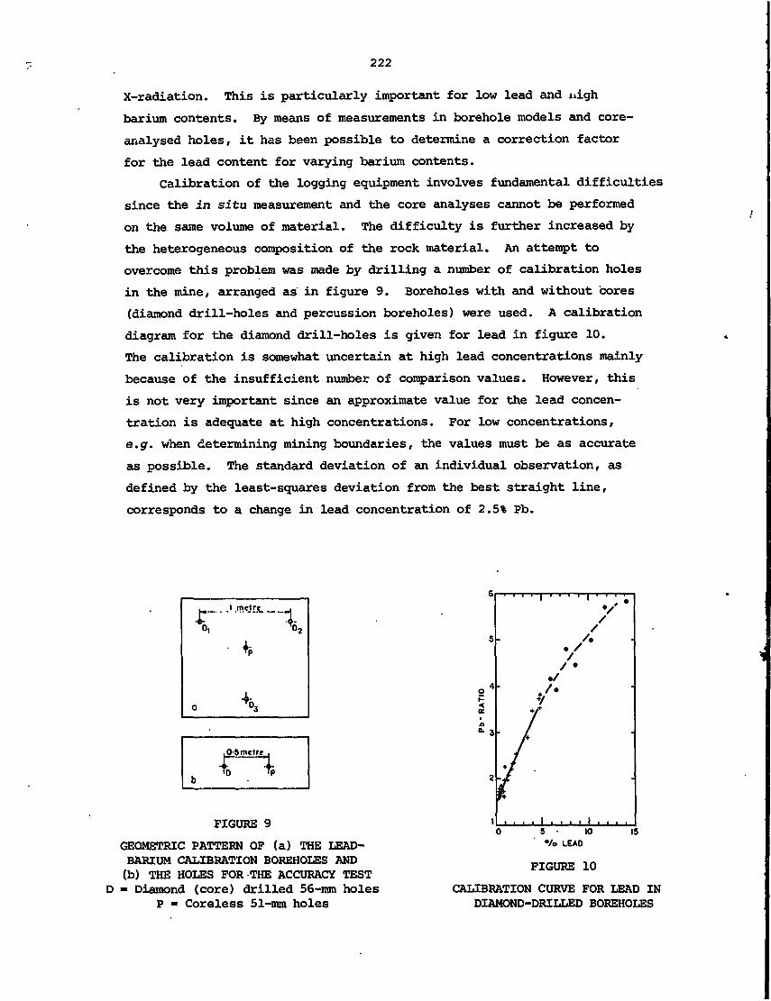
222
X-radiation. This is particularly important for low lead and nigh
barium contents. By means of measurements in borehole models and core-
analysed holes, it has been possible to determine a correction factor
for the lead content for varying barium contents.
Calibration of the logging equipment involves fundamental difficulties
since the in situ measurement and the core analyses cannot be performed
on the same volume of material. The difficulty is further increased by
the heterogeneous composition of the rock material. An attempt to
overcome this problem was made by drilling a number of calibration holes
in the mine, arranged as in figure 9. Boreholes with and without cores
(diamond drill-holes and percussion boreholes) were used. A calibration
diagram for the diamond drill-holes is given for lead in figure 10.
The calibration is somewhat uncertain at high lead concentrations mainly
because of the insufficient number of comparison values. However, this
is not very important since an approximate value for the lead concen-
tration is adequate at high concentrations. For low concentrations,
e.g. when determining mining boundaries, the values must be as accurate
as possible. The standard deviation of an individual observation, as
defined by the least-squares deviation from the best straight line,
corresponds to a change in lead concentration of 2.5% Pb.
I metre
b
. 0-5 metre .
FIGURE 9
GEOMETRIC PATTERN OF (a) THE LEAD-BARIUM CALIBRATION BOREHOLES AND(b) THE HOLES FOR THE ACCURACY TEST
D = Diamond (core) drilled 56-mm holesP = Coreless 51-mm holes
FIGURE 10
CALIBRATION CURVE FOR LEAD INDIAMOND-DRILLED BOREHOLES

223
On the assumption that the calibration curves for the diamond
drill-holes also apply for the coreless production holes, a number of
holes of each kind were logged and the lead concentrations calculated.
These concentrations were then compared with the corresponding results
from core analyses. A list of some of these measurements and analyses
is given in table 1. The discrepancies noted are not greater than can
be explained by the heterogeneous-mineralisation. From this it can be
concluded that the concentration values for lead obtained by the radio-
isotope X-ray fluorescence method are as reliable as those obtained by
core-drilling and analysis. Furthermore, the logging technique is much
quicker and it enables a very detailed investigation of the borehole
profile to be made, even in coreless holes.
TABLE 1
CALCULATED MEAN LEAD CONCENTRATION IN AN ANALYSED ZONE IN THE LAISVALL MINE(Comparison between core and in situ analyses)
Borehole Analysed Zone(m)
1435 0.00 - 11.48
1436 7.10 - 9.860.00 - 11.54
1437 0.00 - 4.790.00 - 6.07
1438 0.00 - 11.01
1439 0.00 - 11.04
1440 0.00 - 8.910.00 - 12.07
Calculated Mean Concentration ofLead (%) in the Analysed Zone from:
Core Analysis
2.56
2.521.20
1.782.16
7.18
0.45
0.361.12
in situ AnalysisDiamond-drilled Hole
2.44
2.31
1.93
6.76
0.46
0.42
in situ AnalysisPercussion-drilled Hole
2.10
1.29
2.31
6.03
0.46
1.33
Example 2
Preliminary tests have been made with borehole probes based on high
resolution proportional detectors. This probe, manufactured by Outokumpu
Oy of Finland, can be pushed into boreholes of diameter > 45 mm. Good
agreement has been shown between in situ borehole measurements and
chemical analysis of the bore core (figure 11).

224
5. CONCLUSION
Bench top and portable mineral analysers have become well established
in the mineral industry, and have in some cases replaced more complicated
and expensive X-ray tube/Bragg crystal analysers. There is limited but
increasing use of radioisotope X-ray techniques of analysis for scanning
of bore cores, especially for tin at concentrations greater than 0.1
wt %. The application of radioisotope X-ray techniques to in situ
borehole logging is increasing, and is particularly suited for logging
for tin (Z = 50) and higher atomic number elements.
1O
U
NJ
OO
— Chemical analysisof core
• X-ray analysisof bore hole
5 1O 15
DEPTH (m)
FIGURE 11
COMPARISON OF BOREHOLE EDXRFAND CHEMICAL ANALYSIS
6. BIBLIOGRAPHY
Christell, R., Ljunggren, K. & Landstrom, O. [1976] - Brief Review of
Development of Nuclear Geophysics in Sweden. Proc. Panel on
Nuclear Techniques in Geochemistry and Geophysics, Vienna, 1974,
IAEA, Vienna, pp. 21-45.
Clayton, C.G. [1976] - Some Experience with the Use of Nuclear Techniques
in Mineral Exploration and Mining. Proc. Panel on Nuclear Techniques
in Geochemistry and Geophysics, Vienna, 1974, IAEA, Vienna, pp. 109-
128.
225
Clayton, C.G. [1977] - Some Recent Applications of Nuclear Techniques
in the Exploration and Mining of Metalliferous Minerals. Proc.
Symp. Nuclear Techniques and Mineral Resources, IAEA, pp. 185-213.
Donhoffer, O.K. [1979] - A Survey of Commercial EDXRF and NDXRF
Instrumentation. Proc. Advisory Group Meeting on Practical Aspects
of Energy Dispersive X-ray Emission Spectrometry, Vienna, 1978,
IAEA-216, pp. 1-13.
Rautala, P., Hietala, M. & Sipila, H. [1979] - Application and
Economic Aspects of WDXRF AND EDXRF Techniques in Industry. Proc.
Advisory Group Meeting on Practical Aspects of Energy Dispersive
X-ray Emission Spectrometry, Vienna, 1978, IAEA-216, pp. 119-134.
Rhodes, J.R. [1971] - Design and Application of X-ray Emission
Analysers using Radioisotope X-ray or v-ray Sources. In Energy
Dispersion X-ray Analysis ; X-ray and Electron Probe Analysis.
American Society for Testing and Materials (ASTM), Special
Technical Report 485, pp. 243-285.

227
CHAPTER 6
BULK ANALYSIS AND SAMPLING
A Series of Lectures'
M. Borsaru
R.J. Holmes
B.D. Sowerby

229
PART A
GAMMA-RAY METHODS
by
B.D. Sowerby

231
1. INTRODUCTION
The overall accuracy that can be achieved in any analytical procedure
depends on cumulative errors in sampling, sample preparation and analysis.
Analysis techniques using penetrating radiation can be applied to the
measurement of average element concentrations over relatively large
volumes of sample. Bulk analysis techniques can therefore be used to
avoid the sample preparation errors usually associated with conventional
chemical analysis. As well, bulk analysis techniques can be used in on-
line applications to reduce significantly the sampling error.
Suitable bulk analysis techniques usually employ either neutrons or
y-rays to achieve adequate sample penetration. In this lecture, we deal
with y-ray methods of bulk analysis which covers both y-ray induced
reactions, selective y-ray scattering and methods which rely on natural
radioactivity.
2. NATURAL GAMMA RADIATION
Where applicable, natural y-radiation forms the basis of a very
simple method of bulk analysis. If one is confronted with a problem of
distinguishing between two components in a sample, one of which is of
high natural radioactivity and the other of low radioactivity, a simple
Y-ray count may be a sufficiently accurate analysis method.
All rocks and soils emit y-rays, primarily from the natural radioelements
«tOK/ 238u and 232Tn> The average abundance of natural radioelements in
various rock is discussed by J. Aylmer in his lecture on natural y-
spactroscopy for borehole logging (see Chapter 7, Part A). Rocks of
high natural y-activity include acid rocks and common shales, and those
of low activity include limestones, non-shaly sandstones, coal, gypsum
and haematite.
Although a large number of energy peaks appear in the natural y-ray
spectra of rocks, the photons of energy 1.46 MeV ( K), 1.76 MeV (21l*Bi)
and 2.62 MeV (208T1) are the most suitable for the measurement of potassium,
uranium and thorium respectively [Wollenberg 1977]'.
As an example of the use of natural y-radiation for analysis, the
natural activity of ** K provides an easy method for quantitatively
measuring the potassium content of minerals. Equipment has been constructed
to assay the potash content in cores [Cameron & Clayton 1971]. Eighteen
Geiger counters, each having an active length of 30 cm, are mounted
around a cylinder through which cores (diameter ~12 cm) are passed.
Twelve metres of core are measured in four hours with an accuracy of
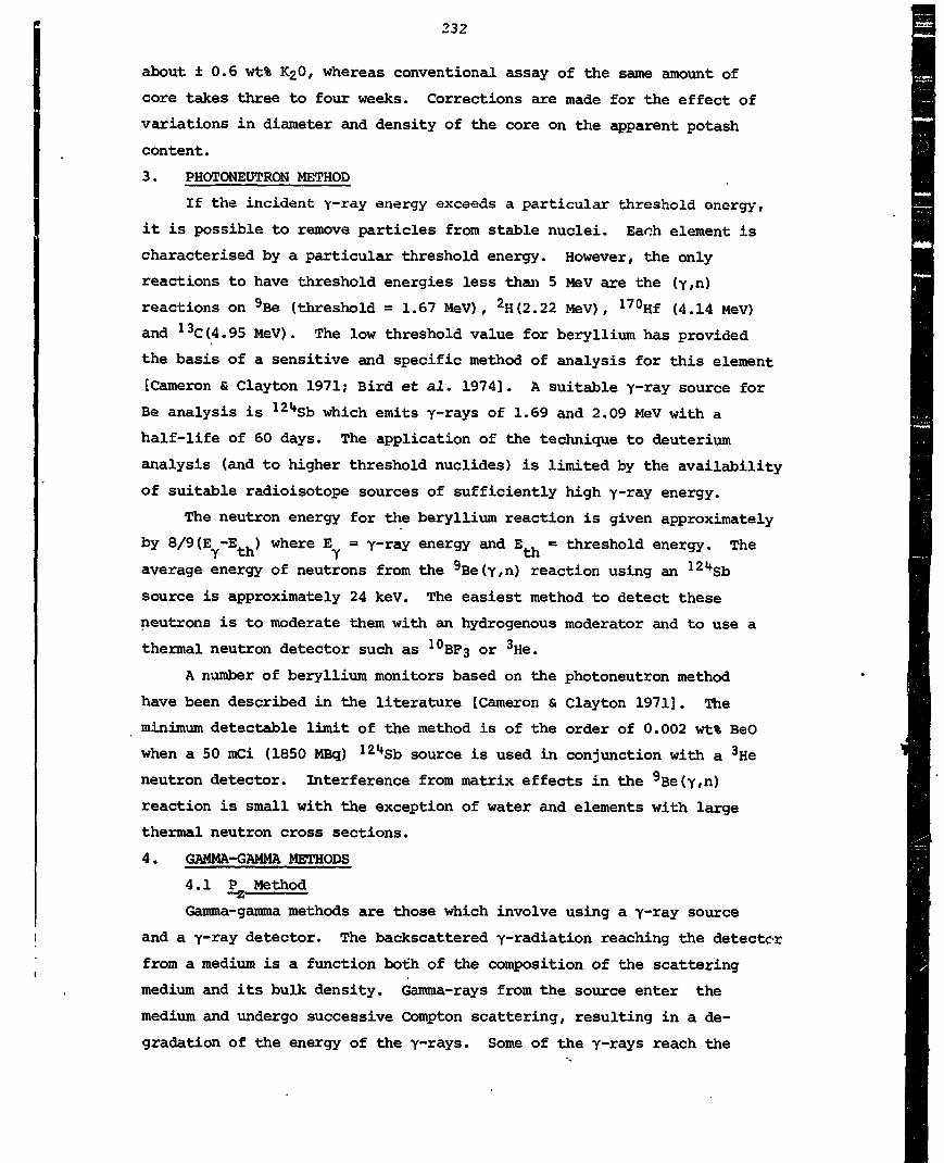
232
about ±0.6 wt% K£0, whereas conventional assay of the same amount of
core takes three to four weeks. Corrections are made for the effect of
variations in diameter and density of the core on the apparent potash
content.
3. PHOTONEUTRON METHOD
If the incident y-ray energy exceeds a particular threshold energy,
it is possible to remove particles from stable nuclei. Each element is
characterised by a particular threshold energy. However, the only
reactions to have threshold energies less than 5 MeV are the (y,n)
reactions on 9Be (threshold = 1.67 MeV), 2H(2.22 MeV), 170Hf (4.14 MeV)
and 13C(4.95 MeV). The low threshold value for beryllium has provided
the basis of a sensitive and specific method of analysis for this element
[Cameron & Clayton 1971; Bird et al. 1974]. A suitable y-ray source for
Be analysis is 12l*Sb which emits y-rays of 1.69 and 2.09 MeV with a
half-life of 60 days. The application of the technique to deuterium
analysis (and to higher threshold nuclides) is limited by the availability
of suitable radioisotope sources of sufficiently high y-ray energy.
The neutron energy for the beryllium reaction is given approximately
by 8/9(E-E) where E = y-ray energy and E « threshold energy. The
average energy of neutrons from the 9Be(y,n) reaction using an 12l*Sb
source is approximately 24 keV. The easiest method to detect these
neutrons is to moderate them with an hydrogenous moderator and to use a
thermal neutron detector such as 10BF3 or 3He.
A number of beryllium monitors based on the photoneutron method
have been described in the literature [Cameron & Clayton 1971]. The
minimum detectable limit of the method is of the order of 0.002 wt% BeO
when a 50 mCi (1850 MBq) 12t*Sb source is used in conjunction with a 3He
neutron detector. Interference from matrix effects in the 9Be(y,n)
reaction is small with the exception of water and elements with large
thermal neutron cross sections.
4. GAMMA-GAMMA METHODS
4.1 P Method—zGamma-gamma methods are those which involve using a y-ray source
and a y-ray detector. The backscattered y-radiation reaching the detector
from a medium is a function both of the composition of the scattering
medium and its bulk density. Gamma-rays from the source enter the
medium and undergo successive Compton scattering, resulting in a de-
gradation of the energy of the y-rays. Some of the y-rays reach the

detector after single Compton scattering, whereas others suffer multiple
Compton scattering before reaching the detector or they undergo photoelectric
absorption. The probability of photoelectric absorption becomes significant
only after the 1-ray energy falls below about 200-300 keV.
In the high energy region of the backscattered gamma-ray spectrum
(i.e. above about 300 keV), Compton scattering is dominant and therefore
the response is a function of electronic density or bulk density of the
medium. Below 300 keV, both Compton scattering and photoelectric absorption
are important and the response is a function of both density and chemical
composition.
It is convenient to define the P ratio asz
Intensity of scattered y-xays in thehigh energy region of the spectrum
P =zIntensity of scattered yrays in thelow energy region of the spectrum
It has been demonstrated, both theoretically and experimentally, that
the P function is dependent on Z (the 'equivalent atomic number1 ofZ ®Q
the medium) and independent of changes in bulk density. The equivalent
atomic number characterises the 'average1 chemical composition of the
medium. For a more complete description of the theory of the Pzmethod, refer to the lecture by P.J. Mathew (Chapter 7, Part B).
4.2 Application to Iron Ore Analysis
As an example of the use of the P method for bulk analysis, the2
application of the method to the analysis of iron ores is discussed
[Holmes 1976]. In the special case of high grade iron ore where a heavy
element (Fe) is dominant, Z and consequently P are directly correlated6C£ Z
with the Fe concentration. It should be noted, however, that in this
case the method can only be employed to measure Fe. Impurities in the
Fe ore, such as silica and alumina, cannot be determined by this technique.
Some knowledge of the other ore constituents is also required before the
technique can be applied to a particular iron ore. For example, an ore
which is high in manganese (or other elements with high atomic number)
is not suitable since Mn will report approximately as Fe.
Holmes [1976] applied the method to the dry basis grade determination
of bulk samples (25-30 kg) of iron ore. The radiation source was 10 mCi
(370 MBq) 60Co and the detector 51 x 51 mm Nal(Tl), as shown in figure 1.
Samples from various locations were brought to a central laboratory,
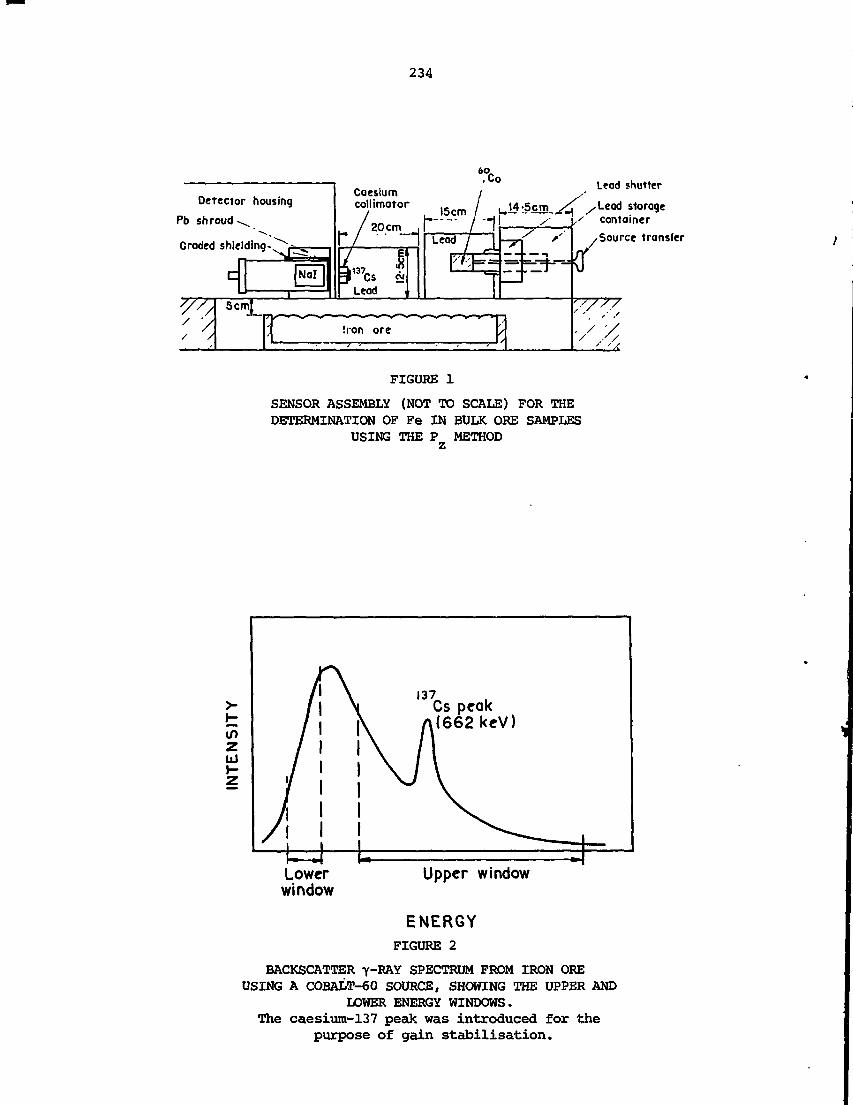
FIGURE 1
SENSOR ASSEMBLY (NOT TO SCALE) FOR THEDETERMINATION OF Fe IN BULK ORE SAMPLES
USING THE P METHODz
234
Lower upper windowwindow
ENERGYFIGURE 2
BACKSCATTER y-RAY SPECTRUM FROM IRON OREUSING A COBALT-60 SOURCE, SHOWING THE UPPER AND
LOWER ENERGY WINDOWS.The caesium-137 peak was introduced for -the
purpose of gain stabilisation.

235
crushed to reduce the particle size to -6 ram and then analysed using the
P technique. A typical backscatter Y~ray spectrum from iron ore iszshown in figure 2. The grade of individual samples was measured to an
accuracy of better than ±0.8 wt% Fe (95 per cent confidence intervals)
with an analysis time of 20 man. This analysis time could be xeduced in
practice by using a larger Nal(Tl) detector.
5. GAMMA-RAY RESONANCE SCATTERING
The y~ray resonance scattering technique can be used for the deter-
mination of copper and nickel in bulk samples and drill cores. The
technique, which is highly specific to the element being measured, has
been developed and field tested by the AAEC [Sowerby et al. 1977]. Bulk
mineral analysers based on Y-ray resonance scattering are now commercially
available from AMDEL.
5.1. Description of Process
Gamma-ray resonance scattering is an elastic process that takes
place via an excited state of a stable nucleus. For a precisely defined
energy of the incident -ray, a stable nucleus can absorb this y~*ay
and become an unstable excited nuclear state. In regaining its stable
state, the nucleus emits a Y~raY of essentially the same energy as that
absorbed. The range of incident Y~ ay energies for which this process
can occur is extremely narrow, typically being 1 or 2 eV for most elements.
Because of the extreme narrowness of this energy range, the process is
entirely specific to the wanted element.
For resonance scattering to be a practical technique of analysis,
a source of the precisely defined Y~ray energy is required. A practical
way to obtain these y-rays is to choose a radioisotope source that
decays via the excited state of the element to be measured. For example,
if the element to be analysed is Ni then a radioactive 60Co source may
be used. This radioisotope decays by (J- and Y~raY emission via excited
states of 6 ONI. Matching the radioactive source to the element being
measured is an essential characteristic of the Y~*ay resonance scattering
analysis technique.
Normally, resonance scattering does not take place when the radio-
isotope source is in the solid state. Recoil energy losses during the
emission and absorption of the source Y~ray cause it to be deficient in
energy by several tens of eV. This deficiency may be overcome by using
a gaseous radioisotope source. Gamma-rays from gaseous sources are
Doppler broadened so that about 1 per cent of the v-rays are in resonance
[Sowerby 1971].

200O
Mineral sample
Incident Jf-rou,
Sliding shutter(open) \ Scattered o"~ray
Nol(Tl) detector
LeadZinc-65vapour source
FurnaceLead —
Slit collimolor
Detector
FIGURE 3
CROSS-SECTIONAL VIEW OF THE BULK ANALYSERINSTALLED AT MOUNT ISA MINES LIMITED.
This analyser is being used to determine the copper contentof crushed bulk samples and drill core. The samplecontainer shown is used for crushed samples of minimum
weight 20 kg. The analyser is calibrated for other samplesizes and for drill core.
Resonance ptotopeo!'.(M2Me/(
O
2SO
to
|5OCH integral) C2 C3 C4 C5
CHANNEL NUMBER
FIGURE 4
PULSE-HEIGHT SPECTRA OBTAINED WITH AMOUNT ISA SAMPLE CONTAINING 3.9 Wt% Cu.
The positions of the windows Cl to C5 are shown.

237
The two most favourable elements for analysis using y-ray resonance
scattering are copper and nickel, using vapour sources of 65Znl2 and60CoBr2 respectively.
5.2 Resonance Scattering Bulk Analyser
A resonance scattering bulk analyser uses a heated gaseous source
and a detector shielded from direct source radiation (figure 3). The
sample is placed over the apparatus and the backscattered radiation is
measured. This backscattered radiation consists of two main components,
due to resonance scattering and Compton scattering. The resonance
scattered yrays are of the full incident energy whereas the Compton
scattered vrays are of much lower energy, being typically about 0.3 MeV.
Pulse-height spectra for a miner?1 sample containing 3.0 wt% Cu are
shown in figure 4.
As resonance scattering does not take place with a solid radioisotope
source, the resonance count rate can be determined by subtracting the
measured count rates for a gaseous and a solid source. In practice
however, the resonance count rate can be determined with sufficient
accuracy by a single measurement with a vapour source. The natural
background under the resonance photopeak is determined by measuring thetf°K, U and Th components using the windows 03, Cij and GS (figure 4) .
Industrial applications usually require the use of source strengths
of about 0.5 to 2 Ci(~15 to 74 GBq) for ores containing 0.2-2 wt% Cu
or Ni. Using these source strengths, analysis times are usually less
than about 5 minutes per sample for a relative accuracy of 5 to 10 per
cent.
Commercial bulk mineral analysers for copper or nickel are expected
to cost about $A50 000, and sources are likely to require annual replacement
at a cost of about $A5000 per year.
5.3 Applications
5.3.1 Crushed Bulk Samples
The resonance scattering technique can be used to measure the
average concentration of copper or nickel in a bulk sample directly
without the need for sample division. Samples for analysis are prepared
by a single pass through a jaw crusher with a jaw opening of about 10
mm; they are then mixed by pouring via an intermediate container. With
this procedure, bulk analyser assays are reproducible to within about ±3
per cent relative, regardless of how the sample is poured into the
sample container.

238
Sample depth should preferably be greater than about 13 cm so that
the sample is infinitely thick with respect to resonantly scattered
y-rays. For thinner samples a thickness correction will be needed. For
crushed bulk samples a small density correction is applied, based on the
count rate of Coiapton scattered y-rays. This correction is a 1.4 per cent
relative change in assay for a 0.1 g cm 3 change in bulk density.
The first field trial of a prototype bulk analyser for copper
determination in bulk samples was carried out in late 1974 at the Mount
Isa Mines Limited site. More than 100 mineral samples of mass 5 to
20 kg were crushed to -25 mm and analysed. The r.m.s. deviations between
bulk analyser and conventional chemical laboratory assays were in the •
range 0.06 to 0.09 wt% Cu (1 standard deviation). More recent laboratory
results on a wide variety of Australian copper and nickel ores have
shown similar r.m.s. deviations.
5.3.2 Drill Core Analysis
The shaped core tray shown in figure 5 enables the bulk analyser to
determine the average copper or nickel content of up to 3 m of drill
core with a single measurement. The core tray is shaped so that contribut-
ions from all parts of the core are approximately equal. The weight of
core on the tray is measured using the intensity of Compton scattered y-
rays. Cores with different diameters are analysed on separate core
trays. The analyser calibration can be checked using Al/Cu alloy bars.
A bulk analyser was installed at the Mount Isa site in mid-1976 for
the routine assay of drill cores and bulk samples. The analyser, which
can be operated by a relatively unskilled person, incorporates a mini-
computer which automatically calculates and displays the copper content
and counting statistical error. A comparison of bulk analyser and
conventional assays shows that, under industrial conditions, the analyser
can measure directly the copper grade over a given length of drill core
with a relative error of less than ± 8 per cent. This performance has
been maintained at Mount Isa for more than three years. The main benefits
of using a bulk analyser in this application are reduced labour requirement,
improved accuracy and a reduced turn-around time for reporting results.

239
FIGURE 5
PHOTOGRAPH OF THE BULK ANALYSER BEFORESHIPMENT TO MOUNT ISA MINES LIMITED.
The equipment is shown analysing a drill core sample.
6. BIBLIOGRAPHY
Bird, J.R., Campbell, B.L. & Price, P.B. [1974] - Atom.Energy Rev., 12
(2) 275.
Cameron, J.F. & Clayton, C.G. [1971] - Radioisotope Instruments. Pergamon
Press, Oxford, Vol.1.
Holmes, R.J. [1976] - Analy.Chem., 48:1155.
Sowerby, B.D. [1971]. Nucl.Instrum. Methods, 94:45.
Sowerby, B.D., Ellis, W.K. & Greenwood-Smith, R. [1977] - In Nuclear
Techniques and Mineral Resources, IAEA, Vienna, p.499.
Wollenberg, H.A. [1977] - In Nuclear Methods in Mineral Exploration
and Production (ed. J.G. Morse), Elsevier, Amsterdam, p.5.

241
PART B
NEUTRON ACTIVATION FOR BULK ANALYSIS
by
M. Borsaru

243
1. INTRODUCTION
The advantage of using large (kg) rather than small (g) samples is
that measurements on large samples eliminate the sample preparation
process, which is both tedious and time consuming and can easily be
affected by errors. The accuracy of conventional laboratory analytical
techniques is critically affected by the extent to which the small
samples used for analysis are truly representative of the bulk. Neutron
activation, a method depending on hard y-rays and neutrons, is preferred
to other bulk sampling methods based on relatively soft X-rays, because
the effective volume of the response sample is substantially enlarged by
the greater penetration of the two hard radiations.
The neutron activation technique is well established as a powerful
tool for the non-destructive analysis of small samples. Its application
to bulk sample analysis requires significant modifications owing to
neutron flux distortions caused by strong neutron absorbers in the ore,
as well as the moderating effect of hydrogen as water associated with
the ore. Neutron activation is very simple and suitable for industrial
applications. A neutron activation analysis (NAA) system consists of a
sample irradiation facility, a system for transferring samples from the
irradiation area to the detector, and the counting facility which includes
a shielded y-ray detector of high efficiency. Within the shielded
irradiation facility, the sample container must be capable of precisely
reproducing the position of samples. Clearly it is also important that
the sample transfer time is also reproducible.
The y-rays counted are those released by the radioactive nuclei
formed during the activation process. The number of y-ray counts,
N, recorded by the detector is given by
<j>ftcrNN - —r-2- [1 - exp (-At )] exp"At [1 exp (-At!)]
A O
where 4» is the neutron flux; ft is a factor including the solid angle
and the efficiency of the detector; a is the neutron activation cross
section; N is the percentage of the element which needs to be analysed
in the sample; X is the decay constant of the radioactive nucleus
formed during the activation process; t is the irradiation time; t is
the delay between the end of irradiation and the start of counting; and
tj is the counting time.
The neutron source must be chosen to suit the activation process.
Californium-252 is best for thermal neutron activation (n,y), but a
neutron generator or a fast neutron source such as either Pu-Be or

244
Am-Be are recommended in the case of the fast neutron activation re-
actions such as (n,p), (n,2n), etc. In the next section the application
of the neutron activation technique for the determination of M.2°3t
Si02 and Mn in different matrixes is discussed. Since the abundances of
Al and Si in the Earth's crust are 8.2 and 25.7 per cent, respectively,
a method capable of measuring the alumina and silica concentrations in
bulk samples of different ores and minerals will find -any applications.
2. TYPICAL USES OF THERMAL NEUTRON ACTIVATION
2.1 The Determination of Alumina in Bulk Samples
The method is based on the thermal neutron reaction 27Al(n,y)28 Al
which has a cross section of 230 millibams. The radioactive isotope28A1 formed in this process has a half-life of 2.3 min and decays by
emitting a 1.78 MeV y-ray. The bulk samples can be irradiated from
underneath in a rectangular box (approximately 8 cm deep) by thermalised
neutrons.
The experimental rig is shown in figure 1. The thermalised neu-
trons are produced by a 252Cf neutron source (between 20 and 50 yg)
located at the bottom of a 10 x 9 cm deep hole drilled into a poly-
ethylene block which, in turn, is surrounded by paraffin bricks. A 15
cm long neutron detector (4 atm 3He) is attached to this assembly below
the sample box to measure the thermal neutron flux in the vicinity of
the ore sample. A sheet of Silastic, impregnated with 10B and suitably
shaped, serves as a shield for the detector against those thermal neu-
trons emitted directly from the thermalising source assembly. A thick
paraffin block located above the sample is used as a reflector of neu-
trons transmitted from the sample. After irradiation, samples can be
rapidly transferred along a small railway track to a position immediately
above the scintillation detector for counting. Background radiation
from the source is reduced by using a thick lead shield around the
scintillation detector. Spectrum stabilisation is always needed when
using a Nal(Tl) detector because the gain is sensitive to variations in
temperature.
Alumina in Bulk Iron Ore Samples
[Borsaru & Holmes 1976]
An activation spectrum of alumina in iron ore is shown in figure 2.
The neutron activation assays are obtained from an equation of the form
y = A + BY + CW + Dn (1)
where y is the NAA assay, y is the number of y~raY counts (thousands) in

245
Nol (TJ) gommo-roydetector.
\
Lead
252
Bismuth -
High-densitypolyethylene
Paraffin
BauxiteSrass box
Neutrondetector
Paraffin
Boron-impregnatedparaffin
FIGURE 1
IRRADIATION AND COUNTING FACILITY EMPLOYINGTHE CALIFORNIUM NEUTRON SOURCE
tnzU)h-z
0 0-5 1-0 1-5 2-0
GAMMA-RAY ENERGY(McV)
FIGURE 2
TYPICAL GAMMA-RAY SPECTRUM RESULTINGFROM THERMAL NEUTRON ACTIVATION OF IRON ORE

0 1 2 3 4 5 6 7
% Aft03 , CHEMICAL ANALYSIS
FIGURE 3
COMPARISONS OF NEUTRON ACTIVATION ASSAYSFOR A1203 WITH CHEMICAL ANALYSIS IN BULK
IRON ORE SAMPLES
SO 52 54 56 58 6O 62 64
°/oALUMINA,CHEMICAL ANALYSIS
FIGURE 4
COMPARISON OF THERMAL NEUTRON ACTIVATIONASSAYS FOR A1203 WITH CHEMICAL ANALYSIS FOR
35 DRIED BAUXITE SAMPLES
246

the 1.78 MeV alumina peak, W is the weight of the sample and n is the
number of thermal neutrons measured underneath the sample. The con-
stants A,B,C and D are determined by regression of the data against
accurate chemical analysis. Figure 3 shows the comparison of neutron
activation assays for A12O3 with chemical analysis. Typically, the
standard deviation obtained from a series of measurements was a = 0.15%
Al£03. When no neutrons were considered in the regression equation (1),
the standard deviation bscair.e 0.19°= A^O^. Tho alirnina concentration in
the bulk iron ore samples (- 25 kg) was in the range 1 to 6% A12O3.
Alumina in Bulk Bauxite Samples
[Borsaru & Eisler 1981]
The accuracy of a measurement given by equation 1 is a = 0.5%
A1203 for the alumina grade in the bulk samples (- 17 kg) ranging from
50 to 60 per cent A^OS. To obtain this accuracy, it is essential to
monitor variations of the neutron flux. There is no need to dry the
samples before the measurement. Figure 4 shows an X-Y plot of assayed
against predicted alumina grades.
Alumina in Bulk Coal Samples
[Borsaru & Mathew 1980]
Alumina is one of the main components of the ash in coal. Thermal
neutron activation can be employed to determine the alumina concentration
in bulk coal samples. A typical accuracy is a = 0.2% Al2C>3 for alumina
concentrations in the range 1 to 10 per cent. There is no need to crush
the samples to a powder or to dry them below 6 per cent free moisture.
Figure 5 shows an X-Y plot of assayed against predicted alumina grades.
2.2 The Determination of Manganese and Alumina in Manganese Ore
The same experimental rig can be used to determine manganese and
alumina in manganese ore. The thermal neutron activation reaction in Mn
has a cross section of 13.3 barns and is as follows:
55Mn + n •*• 56Mn
The radioactive isotope 56Mn has a half-life of 2.6 hours and decays by
emitting y~radiations at energies of 0.847, 1.811 and 2.113 MeV. The
1.8 MeV Y-ray peak resulting from the decay of the radioisotope 28Al
cannot be separated from the 1.811 MeV j-ray peak resulting from the
decay of 56Mn. Manganese concentration is determined from the intensity
of the 2.113 MeV peak. The alumina concentration is measured from the
1.8 MeV Y~raY peak after correcting for the interference from manganese.

248
12
1O
P 8U
I
44
1 1 12 4 6 8 1 O
°/o Af 2 O 3 X-RAY FLUORESCENCE
FIGURE 5
COMPARISONS OF NEUTRON ACTIVATION ASSAYSFOR A12O3 WITH CHEMICAL ANALYSIS IN BULK
COAL SAMPLES
12
/NoKTf) gommo-ray/detector
/Mini-rails
. ,
/Bauxite
Brass box
I!
AAm-Be neutron source
Neutron detector
FIGURE 6
IRRADIATION AND COUNTING FACILITYEMPLOYING THE Am-Be NEUTRON SOURCE

249
The intensity of the 1.811 MeV y-radiation from 56Mn can be estimated by
multiplying the intensity of the 2.113 MeV peak by a constant. This
constant is found by comparing the 1.811 MeV peak with the 2.113 MeV
peak 20 minutes after irradiation, when all the 28A1 activity has de-
cayed.
3. TYPICAL USES OF FAST NEUTRON ACTIVATION
3.1 The simultaneous Determination of silica and Alumina in Bulk
Bauxite Samples
Nuclear reactions 27Al(n,p)27Mg and 28si(n,p)28Al are used, respect-
ively, for the determination of alumina and silica. The bauxite bulk
samples are also irradiated from underneath in a shallow rectangular
brass box (figure 6) by an Am-Be neutron source (activity: 10 to 20 Ci
(370 to 740 MBq)). A 3He/Kr neutron detector (4 atm) is located beneath
the sample box adjacent to the source to monitor changes of the thermal
neutron flux within the bulk sample.
The radioactive nucleus produced by the first reaction, 27Mg,
decays with a half-life of 9.46 min and, during its decay, emits two y-
rays which have energies of 0.844 and 1.055 MeV. The alumina grade (Al)
is related to the number of y-rays, G, emitted by 27Mg at 0.844 MeV, and
the sample weight, W, by
Al = a +• bG + cW + dC (2)
where the parameter C represents the number of counts observed in the
1.78 MeV y-ray peak within a. preset time. The constants of the equation
are a,b,c, and d. Because the Compton tail of this peak, which is of
variable area, stretches into the counting window set around the 0.844
MeV peak, its contribution must be subtracted by means of the term 'dC1
in the regression equation. It was found that the standard deviation of
the method is a = 0.9% Al20s and that it is independent of both particle
size and the amount of free moisture in the sample.
Because of collisions with the hydrogen nuclei din the bulk samples,
a large number of fast neutrons are thermalised and then induce the
nuclear reaction 27Al(n,y)28Al. It is not possible to differentiate
between the 28A1 radioactive nuclei formed by this reaction and those
formed by the 28Si(n,p)28Al reaction. This problem of interference does
not arise when small samples are irradiated since they contain insuff-
icient hydrogen to moderate the fast neutrons. A new method which
allows for the alumina interference in the silica determination of bulk
bauxite samples has recently been developed. The y-ray counts recorded

250
in the 1.78 MeV peak are produced from the products of the 2p3i(n,p)28Al
and 27Al(n,Y):i8Al reactions. In other words, G tot Si GA1' Where
in a given time, G is the total number of y-rays recorded in the 1.78
MeV peak, G . is the number of y-rays recorded in the 1.78 MeV peak due
to the 28Si(n,p)28Al reaction and G , is the number of y-rays observed
in the 1.78 MeV peak due to the ?7A1(n,>)-^Al reaction. G is pro-
portional to both the thermal neutron flux, <j> ., in the bulk samples and
the percentage Al2O3, the alumina grade of the sample, i.e.
A1 *th Al2°3
It is assumed that the number of thermal neutrons, n, measured by
the 3He neutron detector underneath the bulk sample, is proportional to
the neutron flux in the sample. The alumina grade of the sample is
proportional to G1, the number of y-rays in the 0.844 MeV peak. The
chemical concentration of silica is related to the parameters described
above by
Si - a1 + d1 Gto + g' (n x G1) + c'w (4)
where a1, c', d' and g' are constants of the equation.
The standard deviation of this method, measured on bulk bauxite
samples (- 3.5 kg) with silica concentrations ranging from 2 to 10 per
cent, is cr = 0.25 % Si02 and is not affected by the particle size or the
free moisture content of the samples. Figure 7 shows an X-Y plot of
assayed against predicted silica content for this case.
3.2 Determination of Silica in Bulk Iron Ore Samples
[Borsaru & Holmes 1978]
The fast neutron reaction 28Si(n,p)28Al can also be employed for
the determination of silica in bulk (- 30 kg) iron ore samples. The
interference from the 27Al(n,y)28Al reaction was found to be minimum in
this case. The standard deviation of the measurement was a = 0.17% Si02for silica concentration in the samples from 1 to 10 per cent.
4. ON-STREAM NEUTRON ACTIVATION SLURRY ANALYSER
[Taylor & Rhodes 1979; Blake et al. 1971-72]
The simplified diagram of an on-stream neutron activation slurry
analyser (NOLA) is shown in figure 8. The unit was developed by Texas
Nuclear Division of the Nuclear-Chicago Corporation for the measurement
of silica in iron ore concentrate slurry. The method employs the fast
neutron reaction 28Si(n,p)28Al. A sample slurry of about 2 L is de-
livered to the holding tank on the analyser. It is then drawn into the

I I I2 4 6 8 1O 12
°/o SILICA.CHEMICAL ANALYSIS
FIGURE 7
COMPARISON OF NEUTRON ACTIVATION ASSAYSFOR SiO2 WITH CHEMICAL ANALYSIS FOR 52
DRIED BAUXITE SAMPLES
Slurry pump(
Neutron sourc
Shield
°/o SiOa analog signal.to control loop
Control and dataacquisition unit
Density gauge
FIGURE 8
SCHEMATIC DIAGRAM OF THE ON-STREAMNEUTRON ACTIVATION SLURRY ANALYSER (NOLA-1)
Fe detector
/Thermal neutron/ detector
^Boron shielding
/Boral
I37_/ Cs sources
/ Aluminium/detector
Paraffin .'* "
— Cf neutron source
- Source manipulation coble
Concrete shielding
10en
FIGURE 9
SCHEMATIC DIAGRAM OF ON-STREAM ANALYSERFOR IRON ORE

252
analyser tube through a two-way valve. When the loop is completely
filled with about 650 mL of slurry, the valve closes and the slurry is
circulated. The slurry is activated as it flows via a 16-turn glass
tube coil past a Pu-Be neutron source. Typically, the standard deviation
of this method is a = 0.10% Si02 for silica concentrations in the range
3 to 11 per cent.
5. ON-STREAM ANALYSIS OF IRON ORE
[Holmes et al. 1978; Holmes et al. 1980]
A neutron irradiation technique has been developed for the simult-
aneous determination of the iron and aluminium content of iron ore fines
(-6 mm particle size) on a moving conveyor belt. The determination of
aluminium is based on thermal neutron activation. As discussed above,
the determination of iron is based on measurement of the prompt y-rays
emitted by Fe in the thermal neutron capture process. The schematic
diagram of the on-stream analyser is shown in figure 9. The belt speed
is 3 m min~1. The accuracy for the determination of alumina was a =
0.12% A12O3 for the average grade of 1500 kg ore samples. A 50 yg252Cf neutron source is employed.
6. BEST METHODS FOR DETERMINING SOME IMPORTANT ELEMENTS
Thermal Neutron Activation
Sodium
Aluminium
Chlorine
Vanadium
Scandium
Manganese
Cobalt
Copper
Selenium
Bromine
Rubidium
Rhodium
Silver
Iridium
Magnesium
Potassium
Calcium
Titanium
Molybdenum
Ruthenium
7. COMMERCIAL ORE-ANALYSERS
Palladium
Iodine
Tungsten
Iridium
Platinum
Rare Earths
Actinides
Fast Neutron Activation
Fluorine
Silicon
Phosphorus
Chromium
Yttrium
Barium
Hafnium
Gold
EMPLOYING NEUTRON ACTIVATION
An automatic activation bauxite analyser MTA-1527 is manufactured
in Hungary. This instrument has proved to be reliable and has been used
effectively to determine silica and alumina in various bauxite ores.
.The sample weight is about 10 g.

253
The Texas Nuclear Division of Ramsey Engineering also manufactures
neutron activation analysers: NALA 1 (Neutron Analytical-Lab Analyser)
and NOLA 1 (Neutron Activation Analysis for Industrial Process Control).
Some of the more important elements that can be measured by NALA are
aluminium, barium, bromine, chromium, gold, fluorine, iridium, iodine,
iron, sjanganese, phosphorus, silicon, sodium, vanadium, and rare earths.
The sample size is normally 100 to 200 g.
A neutron activation analyser employing bulk samples (kg) is being
developed in Australia.
8. BIBLIOGRAPHY
Blake, K.R., Ashe, J.B., Berry, P.P. & Nelson, J.B. [1971-72] - Isot.
Radiat. Technol., 9:167.
Borsaru, M. & Holmes, R.J. [1976] - Anal. Chem., 48:1699.
Borsaru, M. & Holmes, R.J. [1978] - Anal. Chem., 50:296.
Borsaru, M. & Mathew, P.J. [1980] - Anal. Chim. Acta, 118:109.
Borsaru, M. & Eisler, P.L. [1981] - Int. J. Appl. Radiat. Isot.,
32:43.
De Soete, D.r Gijbels, R. & Haste, J. [1972] - Neutron Activation
Analysis; Chemical Analysis. Monographs on Analytical Chemistry
and its Applications, Vol. 34, Wiley Interscience, New York.
Erdtmann, G. [1976] - Neutron Activation Tables. Kernchemie in
Einzeldarstellungen, Vol. 6.
Holmes, R.J., Borsaru, M. & Wylie, A.W. [1978] - Australas. Inst.
Min. Metall. Conference, North Queensland, September.
Holmes, R.J., Messenger, A.J. & Miles, J.G. [1980] - Proc. Australas.
Inst. Min. Metall., No. 274:17.
Leniham, J.M.A., Thomson, S.J. & Guinn, V.P. (eds.) [1972] - Advances in
Activation Analysis. Academic Press, New York.
Taylor, M.C. & Rhodes, J.R. [1979] - Instrum. Technol., 21:32.

255
PART C
PROMPT NEUTRON-GAMMA METHODS
by
B.D. Sowerby

257
1. INTRODUCTION
Two methods of bulk analysis use a radioisotope neutron source and
detection of prompt y-rays - namely neutron inelastic scatter and thermal
neutron capture. Fast neutrons interact with matter to yield prompt
y-rays primarily from neutron inelastic scattering. Once the neutrons
are slowed down, prompt y-rays are produced principally by thermal
neutron capture.
Both techniques have the advantage of using penetrating radiation,
so average elemental concentrations are obtained over a large volume of
sample. Also, both techniques are suited to multi-element analysis
although accuracy depends on interelement interferences and background.
2. NEUTRON INELASTIC SCATTER
2.1 Description of Process
Neutron inelastic scattering occurs when a neutron gives up some of
its energy to the nucleus with which it collides, leaving it in an
excited state. The nucleus then decays to a stable ground state by the
prompt emission of one or more y-rays. The process is characterised by
a threshold energy above which the cross section rises with increasing
neutron energy. Different y-rays from various nuclei have different
inelastic scattering thresholds. The neutron inelastic scattering
process is generally important only for neutron energies above about 0.5
to 1 MeV.
The neutron inelastic scattering reaction is written in the form
A(n,n1y)A. The y-rays originate in the nucleus and are relt:-ed to its
nuclear level structure. Each nucleus has its own characteristic set of
neutron inelastic scatter y-rays. A list of the measured photopeak
count rates of some prominent neutron inelastic scatter y-rays is given
in table 1. Many elements yield y-rays in the 0.75 to 3 MeV region and
therefore gamma-ray spectra are often fairly complex and interelement
interferences can be a problem. Also, as the cross section for inelastic
scatter is of the same order of magnitude for many of the common elements,
the technique is most suitable for the analysis of major constituents
(i.e. greater than about 2 wt%) in a sample.
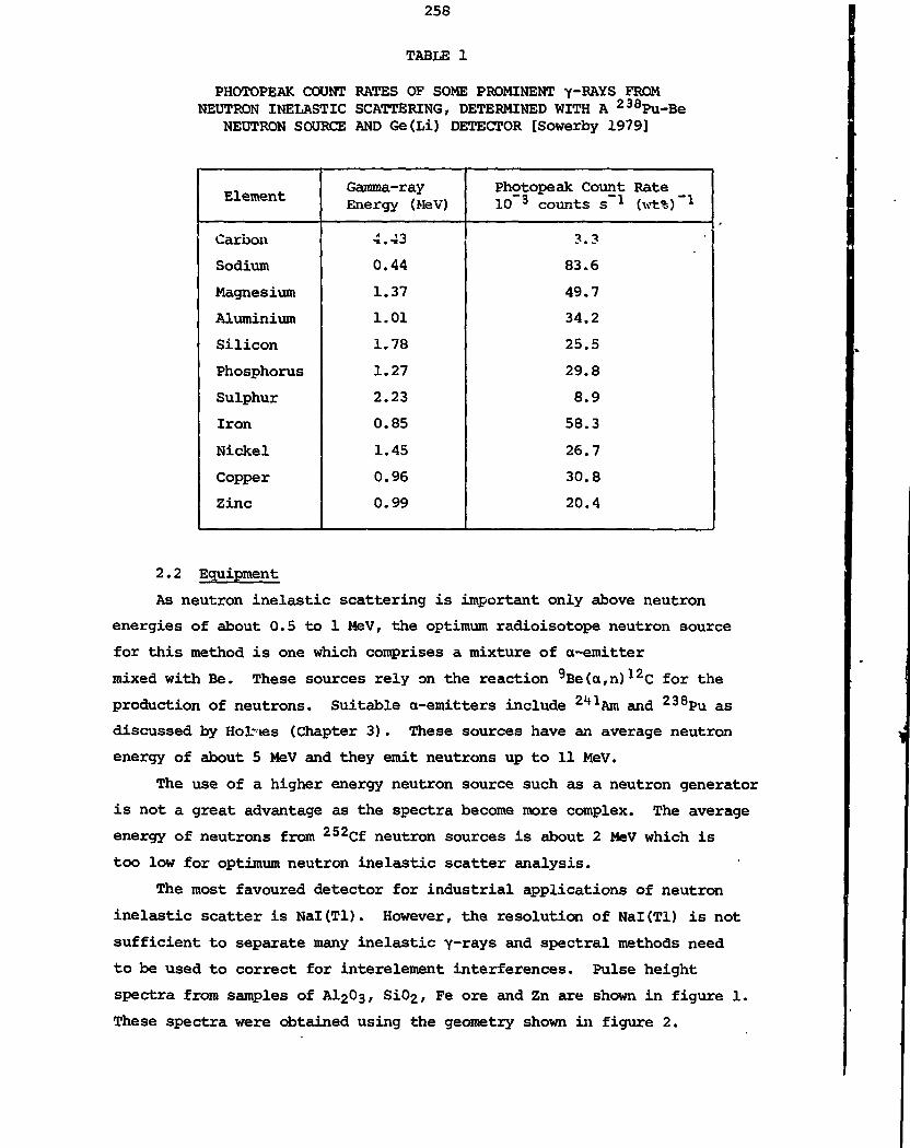
258
TABLE 1
PHOTOPEAK COUNT RATES OF SOME PROMINENT y-RAYS FROMNEUTRON INELASTIC SCATTERING, DETERMINED WITH A 238Pu-Be
NEUTRON SOURCE AND Ge(Li) DETECTOR [Sowerby 1979]
Element
Carbon
Sodium
Magnesium
Aluminium
Silicon
Phosphorus
Sulphur
Iron
Nickel
Copper
Zinc
Gamma-rayEnergy (MeV)
4.43
0.44
1.37
1.01
1.78
1.27
2.23
0.85
1.45
0.96
0.99
Photopeak Count Rate10~3 counts s~l (wt*)"1
3.3
83.6
49.7
34.2
25.5
29.8
8.9
58.3
26.7
30.8
20.4
2.2 Equipment
As neutron inelastic scattering is important only above neutron
energies of about 0.5 to 1 MeV, the optimum radioisotope neutron source
for this method is one which comprises a mixture of a-emitter
mixed with Be. These sources rely on the reaction 9Be(ct,n)12C for the
production of neutrons. Suitable a-emitters include 2ltlAm and 238pu as
discussed by Hol-ies (Chapter 3). These sources have an average neutron
energy of about 5 MeV and they emit neutrons up to 11 MeV.
The use of a higher energy neutron source such as a neutron generator
is not a great advantage as the spectra become more complex. The average
energy of neutrons from 252Cf neutron sources is about 2 MeV which is
too low for optimum neutron inelastic scatter analysis.
The most favoured detector for industrial applications of neutron
inelastic scatter is Nal(Tl). However, the resolution of Nal(Tl) is not
sufficient to separate many inelastic "{-rays and spectral methods need
to be used to correct for interelement interferences. Pulse height
spectra from samples of Al2^3> Si02, Fe ore and Zn are shown in figure 1.
These spectra were obtained using the geometry shown in figure 2.
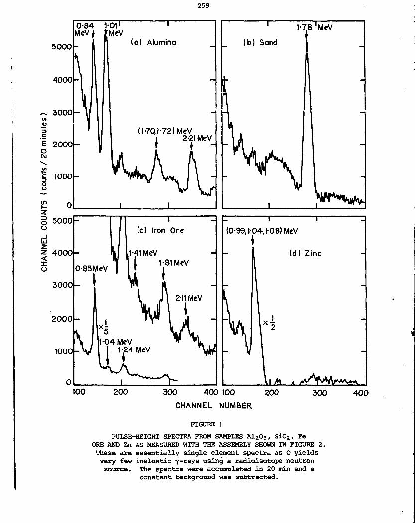
259
5000
4000
~ 3000
3
'ioCM
W
IO
Oo
UJ
<o
2000
1000
0
5000
4000
0-84MeVf
(a) Alumina
(1-70,1-72) MeV1 2-21 MeV
* * -
1 1-78 'MeV
3000-
2000
1000
0-85MeV
(c) Iron Ore
1-81 MeV
1-04 MeV1-24 MeV
2-11 MeV
(0-99,1-04,1-08) MeV
(d) Zinc
100 200 300 400 100
CHANNEL NUMBER
200 300 400
FIGURE 1
PULSE-HEIGHT SPECTRA PROM SAMPLES A^Os, SiO2, FeORE AND Zn AS MEASURED WITH THE ASSEMBLY SHOWN IN FIGURE 2.These are essentially single element spectra as 0 yieldsvery few inelastic y~rays using a radioisotope neutronsource. The spectra were accumulated in 20 min and a
constant background was subtracted.

Li2 C03
shield
Gamma ray
f.•'.'"'''':'::'-".'/'?:I ••'."•. • • • / • • •
7-6cm x 7-6cmNal (T l )detector
Sample
Incident neutron
238Pu-BeNeutron source
toCT>O
Tungsten leadshield
OI
100
Scale (rnm)
FIGURE 2
CROSS SECTION OF THE EXPERIMENTAL SET-UP FOR THEDETERMINATION OF INELASTIC SCATTER COUNT RATES
USING AN Nal(Tl) DETECTOR.

261
An important source of background in an Nal(Tl) detector is due to
neutron interactions in the crystal. The iodine can capture a thermal
neutron or a fast neutron can make a (n,n1y) reaction with an iodine or
sodium nucleus in the crystal. Neutron capture in 127i not only produces
capture y~rays but also produces 128i (T, = 25 min) which decays predominantly
by 3-emission to the ground state of 128Xe. This g-decay produces a
continuous ramp in the pulse-height spectrum up to about 2 MeV [Shafroth
1967].
High resolution Ge(Li) detectors can be used to resolve most inelastic
scatter y~rays. However Ge(Li) detectors are not suitable for industrial
applications of neutron inelastic scattering because of their low photopeak
efficiency and sensitivity to neutron damage, and the need for cooling
to liquid nitrogen temperatures. Fast neutron damage in Ge(Li) detectors
has been observed to increase peak widths by about 50 per cent when the
total irradiation has reajhed 6 x 10⁸ n cm 2.
The optimum geometry for neutron inelastic scatte: ing is an open
geometry with few materials present, apart from the sample, either to
slow down and thermalise neutrons or to produce unwanted background.
However, the radioisotope source needs to be separated from the detector
by a shield to reduce source y-rays. Suitable materials for this
shield are bismuth and tungsten. As well, the detector should be shielded
from thermal neutrons, preferably using a compound of boron or lithium.
The requirement for an open geometry makes shielding more difficult
in an industrial environment. A typical neutron inelastic scatter gauge
will need to be enclosed in a small blockhouse having approximate minimum
internal dimensions 1.5mxl.5mxl.5m and wall thickness of about 30
cm.
2.3 Applications
2.3.1 Analysis of carbon
Neutron inelastic scattering is a suitable technique for the deter-
mination of carbon in such materials as coal and iron ore sinter.
Carbon yields a high energy 4.43 MeV yray from neutron inelastic scatter
which is relatively free from interference from other inelastic scatter
y-rays. A more complete description of the application of this technique
to the determination of carbon in coal is given in Part D of this series.

262
2.3.2 Analysis of Mg, Al and Fe in sand
Magnesium, aluminium and iron have been determined in sand at
levels of > 1 per cent by inelastic neutron scattering [Pierce et al.
1972]. Neutrons were obtained from a 1 Ci (37 MBq) 210Po-Be source and
y-rays detected in a 7.6 cm x 7.6 cm Nal(Tl) detector. Sample size in
this experiment was about 1 to 2 kg., five per cent iron in a sand
matrix was determined to within about 10 per cent relative.
2.3.3 Analysis of Pb/2n ores
Preliminary investigation into the application of the technique to
the analysis of Pb/Zn ores has been carried out by analysing six samples
of ore from Cobar Mines Pty Ltd, New South Wales, Australia, in the
assembly shown in figure 2 [Sowerby 1979]. The samples each weighed
from 9 to 13 kg and contained up to 7 wt% Pb and 14 wt% Zn. Pulse
height spectra from two of these samples are shown in figure 3. The
spectrum shown as the unbroken line was obtained with a sample having
relatively high Zn, Pb and S, whereas the broken line spectrum was
obtained with one having relatively low Zn, Pb and S but high Si. Both
samples contained similar amounts of Fe. The measured photopeak count
rate of the 1.0 MeV -y-ray showed a good correlation with the Zn content
of the samples [Sowerby 1979].
5OOO
1OO 3OO . 3OO 4OOCHANNEL NUMBER
FIGURE 3
PULSE-HEIGHT SPECTRA FROM TWO SAMPLES OF COBARORE AS MEASURED WITH THE GAUGE SHOWN IN FIGURE 2.The spectra were accumulated with a counting timeof 20 min and a constant background was subtracted.

263
3. NEUTRON CAPTURE GAMMA-RAYS
3.1 Description of Process
Once fast neutrons from a radioisotope neutron source enter a
medium, they undergo collisions by which they lose energy until they
eventually reach the thermal region (~0.025 eV). The predominant process
in this slowing down is clastic scattering. The ir.ean displacement over
which a fast neutron is slowed to thermal energy is called the slowing
down length. The slowing down length is about 7.7 cm in water and 35 cm
in pure quartz.
Once slowed down to thermal energies, neutrons diffuse through the
medium without further loss of energy until another process such as
neutron capture terminates their independence. The diffusion length of
thermal neutrons is approximately 2.3 cm in water and 17 cm in pure
quartz.
In the capture process, the thermal neutron enters the nucleus,
producing a compound nucleus in an excited state which then decays to
the ground state by the emission of one or more y~rays. These y-rays
are characteristic of the particular nucleus and are called neutron
capture y-rays. The process of capture and y-ray emission takes only
about 10 1:i s; this is virtually instantaneous compared to the initial
slowing down and diffusion process which may take several hundred micro-
seconds. The capture process is usually written in the
TABLE 2
ANALYTICAL SENSITIVITIES OF SOME PROMINENT NEUTRONCAPTURE Y-RAYS FROM COMMON ELEMENTS [Holmes et al. 1978]
Element
Carbon
Nitrogen
Aluminium
Silicon
Sulphur
Chlorine
Iron
Nickel
Cross Section(barns)
0.003
0.075
0.235
0.160
0.512
33.2
2.62
4.6
Gamma-rayEnergy (MeV)
4.945
10.828
7.724
4.934
5.420
6.111
(7.632,7.646)
8.999
Sensitivity*
0.019
0.080
0.175
0.402
0.678
14.8
2.31
3.2
*Sensitivity - la/A, where I = number of y-rays of given energy producedper 100 neutrons captured, a = cross section and A = atomic mass.

264
form A(n,y)B. The product nucleus may be stable or it may decay to
another product nucleus, often with 3-particle emission. The overall
process is then referred to as thermal neutron activation.
Most elements yield a large number of capture y-rays [Duffey
et al. 1970] and so y-ray spectra are generally complex and interelement
interferences a problem. Neutron capture y-rays which are important in
bulk analysis generally are in the energy range 4 to 10 MeV. One notable
exception to this is the hydrogen capture y-ray at 2.22 MeV. A list of
the analytical sensitivities of some prominent neutron capture y-rays
is given in table 2.
3.2 Equipment
The most commonly used sources for neutron capture y-ray analysis
are 252Cf or one of the a-Be neutron sources. Compared to a-Be sources,252Cf has the advantages of small physical size, lower cost for higher
source outputs and less interference from inelastic scatter y-rays.
However, its 2.6 year half-life requires that the source be replaced
every few years.
Large Nal(Tl) detectors are generally most suitable for industrial
application of neutron capture y-ray techniques, even though they are
incapable of resolving the many y-rays in a typical spectrum. Ge(Li)
detectors can be used but they suffer from the disadvantages discussed
in section 2.2.
In applications of the neutron capture y-ray technique, maximum
count rates are obtained by maximising the thermal neutron flux in the
sample. The sample or the surrounding assembly should preferably be
large compared to the slowing down lengths and diffusion lengths of
neutrons. The optimum geometry is therefore a closed geometry which
also has the advantage of being well shielded. The overall size (including
shielding) of a neutron capture gauge containing an intense 252cf source
of output 4 x 10⁸ n s 1 could be a cube of side ~2 m.
As for neutron inelastic scatter, the count rates in the peaks of
interest are only a very small proportion of the total count rate in the
detector. Also the background under the peaks is often substantial. It
is therefore necessary to count at high count rates (;> 100 000 counts
s *) to achieve good counting statistics. Counting at high rates requires
the use of fast electronics to maintain resolution and minimise pulse
pile-up.

2G5
3.3 Applications
3.3.1 Analysis of sulphur in coal
Two US laboratories are developing on-line bulk analysis gauges for
the determination of sulphur in coal. Both gauges are based on the
measurement of 5.42 MeV neutron-capture y-rays from sulphur using 252Cf
neutron sources and a large Nal(Tl) detector. These applications are
described more fully in Part D of this s«?rie»s.
3.3.2 Analysis of iron in ore products
Neutron capture y-xay techniques for determination of iron in ore
products are being developed in both Sweden and Australia. In Sweden,
the requirement is to determine iron in haematite ore concentrates
resulting from a dry concentration process based on electrostatic
Scintillation detectorfor eC- radiation
Ilectronics
112341
Reqister
1 1 1 1 1 1 1 1 1
JRecorder
/Signal coble
FIGURE 4
IRON CONTENT ANALYSER BASED ON NEUTRON CAPTURE f-BKYS
precipitation. In Australia, iron and aluminium content is required for
blending high grade iron ore before shipping. In both cases, iron is
determined using a fast neutron source surrounded by a moderator, and
the iron capture y-rays (7.64 MeV) are detected by a scintillation
detector. In the Swedish work [Ljunggren & Christell 1976], a 238Pu-Be
source (4 x 10⁶ n s -1) and detector are used in a transmission geometry
(figure 4), and the height of the concentrates on the conveyor is kept
approximately constant with a cutter. On-line plant trials have demonstrated
that iron in the range 40 to 70 wt% can be determined with a standard
error of 1 wt% in two minutes. The equipment has proved simple to
handle and is practical for industrial use.
In the Australian work [Holmes et al. 1978], both transmission and
backscatter geometries have been investigated. The backscatter geometry
is more suitable when the conveyor is heavily laden and variations in

266
Poroffin
Nol (Tl)gammo-roy detector
IOB impregnated silasticrubber
Bismuth shielding
Pb discBora I sheet
Iron ore
Rubber conveyor beltBi shield
_ _Cf neutron source
Bi capsule
High densitypolyethylene
FIGURE 5
CROSS SECTION OF SOURCE-DETECTORCONFIGURATION FOR DETERMINATION OF Fe
Hi/>
UJ
XI
, * '.--wu/n'V :,
:r.r
0 1 2 3 4 5 6 7 8 9
GAMMA-RAY ENERGY (MeV )
FIGURE 6
TYPICAL THERMAL NEUTRON CAPTURE GAMMA-RAYSPECTRUM FROM IRON ORE.
The photopeak from iron is evident at 7.64 MeV asare the single and double escape peaks at 7.13 and
6.62 MeV respectively.

267
ore depth are considerable. The transmission geometry is more suitable
for fixed ore geometries where the conveyor is lightly laden. The ore
profile is kept reasonably constant either with a levelling bar or by
choke-feeding from a hopper. This method of profiling works well with
fine ore(-6 mm) but is unsatisfactory for lump. A transmission source-
detector configuration is shown in figure 5 and a typical Y~raY spectrum
is shown in figure 6. A 10 yg -J-cf (2 x 10' n s *) is located in a
bismuth capsule and the y-rays are detected in a 76 mm x 76 mm Nal(Tl)
detector.
Compensation must be made for the varying moisture content of the
ore and for variations in weight per unit area of ore on the belt. In
extensive laboratory tests on a static conveyor belt, iron in the range
58 to 67 wt% was determined to within 1.2 wt% (2o) for an analysis time
of about 10 minutes.
4. BIBLIOGRAPHY
Duffey, D., El-Kady, A., Senftle, F.E. [1970] - Nucl.Instrum. Methods,
80:149.
Holmes, R.J. Borsaru, M., Wylie, A.W. [1978] - Aust.lnst.Min. Metall.,
N. Queensland Conference, p.235
Ljunggren, K. & Christell, R. [1976] - Proc.Panel on Nuclear Techniques
in Geochemistry and Geophysics, Vienna 1974. IAEA, Vienna, p.181.
Pierce, T.B., Boswell, C.R. & Haines, K. [1972] - J. Radioanal.
Chcm., 10:83.
Shafroth, S.M. [1967] - Scintillation Spectroscopy of Gamma Radiation,
Gordon and Breach, London, p.143.
Sowerby, B.D. [1979] - Nucl.Instrum.Methods, 166:571.

269
PART D
BULK ANALYSIS OP COAL
by
B.D. Sowerby

1. INTRODUCTION
There is a large potential for making savings by using on-line
analysis techniques in the coal industry, particularly in the control of
coal washeries and in the more efficient operation of coal-fired power
stations. Three important parameters for which on-line analysis is
required are specific energy, ash and moisture. Ash is the oxidised
incombustible residue from the combustion of coal and corresponds closely
to the mineral matter content. Radioisotope X-ray techniques have been
developed for the analysis of the ash content of coal; they are based
on the difference in absorption of X-rays in the coal matter and the
higher atomic number constituents of the mineral matter. Neutron techniques
can be used to measure the concentration of some specific elements such
as C,H,S and Al in the coal. The measurement of specific energy, ash
and moisture then depends on the correlation of the particular parameter
with the measured elemental composition. Sulphur analysis is important
where high S coals are used for power generation.
At the present time, there is much research and development under
way in many parts of the world on the application of nuclear techniques
to the on-line bulk analysis of coal. It is expected that developments
in this field will be rapid during the next five years.
2. ASH ANALYSIS BY RADIOISOTOPE X-RAY TECHNIQUES
2.1 Single X-ray Measurement
The ash content of coal can, in some cases, be determined from a
single measurement proportional to mass absorption coefficient of X-rays
in the coal, in, which can be determined either by transmission or
scatter techniques. This coefficient is expressed in terms of mass
absorption coefficient y. and concentration C. of the i element in the
coal by
yi = E y. .C. (1)i x i
Equation (1) can be simplified to
where y is mass absorption coefficient, C is concentration, subscripts
'am' and 'mm' refer to coal matter and mineral matter respectively, and:
C + C = 1 (3)em mm
Using these equations, the mineral matter content can be determined from
a single measurement proportional to mass absorption coefficient if y
and y are essentially constant. Since mineral matter is closelymm
correlated with ash content, the latter can also be determined.
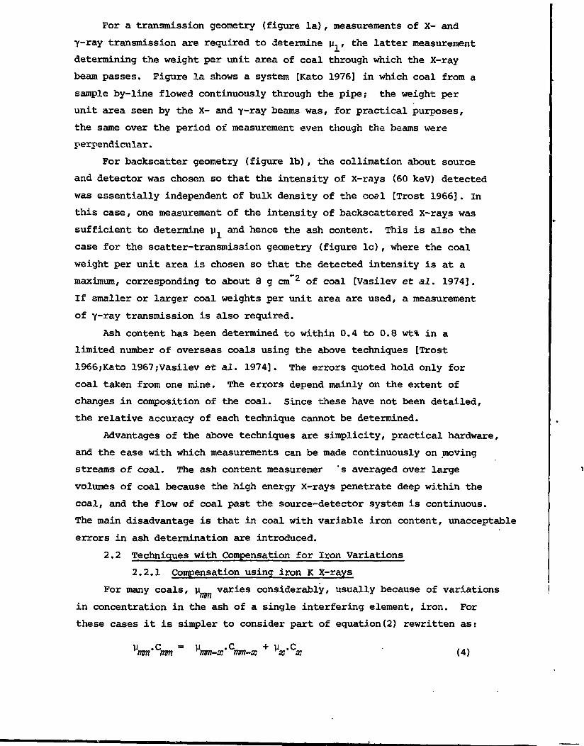
For a transmission geometry (figure la), measurements of X- and
y-ray transmission are required to determine p , the latter measurement
determining the weight per unit area of coal through which the X-ray
beam passes. Figure la shows a system [Kato 1976] in which coal from a
sample by-line flowed continuously through the pipe; the weight per
unit area seen by the X- and yray beams was, for practical purposes,
the same over the period of measurement even though the beams were
perpendicular.
For backscatter geometry (figure Ib), the collimation about source
and detector was chosen so that the intensity of X-rays (60 keV) detected
was essentially independent of bulk density of the COB! [Trost 1966]. In
this case, one measurement of the intensity of backscattered X-rays was
sufficient to determine y. and hence the ash content. This is also the
case for the scatter-transmission geometry (figure Ic), where the coal
weight per unit area is chosen so that the detected intensity is at a
maximum, corresponding to about 8 g cm 2 of coal [Vasilev et al. 1974].
If smaller or larger coal weights per unit area are used, a measurement
of y-*ay transmission is also required.
Ash content has been determined to within 0.4 to 0.8 wt% in a
limited number of overseas coals using the above techniques [Trost
1966;Kato 1967;Vasilev et al. 1974]. The errors quoted hold only for
coal taken from one mine. The errors depend mainly on the extent of
changes in composition of the coal. Since these have not been detailed,
the relative accuracy of each technique cannot be determined.
Advantages of the above techniques are simplicity, practical hardware,
and the ease with which measurements can be made continuously on moving
streams of coal. The ash content measuremer 's averaged over large
volumes of coal because the high energy X-rays penetrate deep within the
coal, and the flow of coal past the source-detector system is continuous.
The main disadvantage is that in coal with variable iron content, unacceptable
errors in ash determination are introduced.
2.2 Techniques with Compensation for Iron Variations
2.2.1 Compensation using iron K X-rays
For many coals, u varies considerably, usually because of variationsHOT?
in concentration in the ash of a single interfering element, iron. For
these cases it is simpler to consider part of equation(2) rewritten as:
vmm'Cmm ~ vmn-x' mm-x + vx'Cx (4)
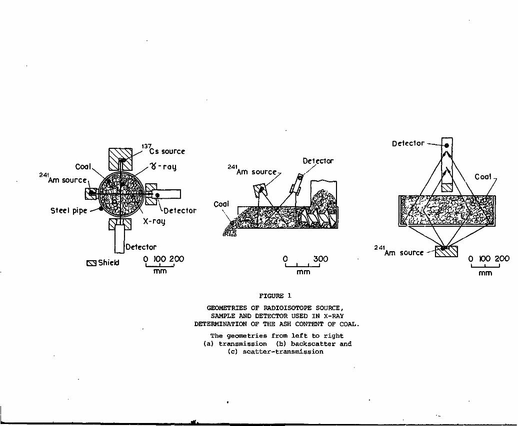
Coal241
Am source
Steel pipe
137Cs source
'b'-ray,
Detector
E3 Shield
Detector
0 100 200mm
Detector
241Detector
Am source
Coal
241
0 300Am source -'
mm
0 KX> 200
mm
FIGURE 1
GEOMETRIES OF RADIOISOTOPE SOURCE,SAMPLE AND DETECTOR USED IN X-RAY
DETERMINATION OF THE ASH CONTENT OF COAL.
The geometries from left to right(a) transmission (b) backseatter and
(c) scatter-transmission
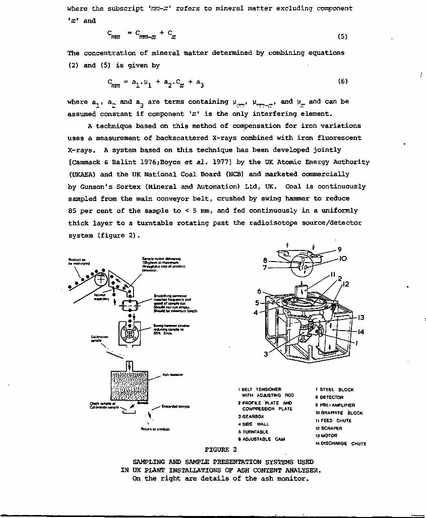
where the subscript 'mxt-z* refers to mineral matter excluding component
'«' and
C c + cwn—x x (5)
The concentration of mineral matter determined by combining equations
(2) and (5) is given by
Cmn = a2'Cx + a3 (6)
where a,, a and a are terms containing y/wi, y , and y^ and can be4. «. O -. . . —». «v
assumed constant if component 'or1 is the only interfering element.
A technique based on this method of compensation for iron variations
uses a measurement of backscattered X-rays combined with iron fluorescent
X-rays. A system based on this technique has been developed jointly
[Cammack & Balint 1976;Boyce et al. 1977] by the UK Atomic Energy Authority
(UKAEA) and the UK National Coal Board (NCB) and marketed commercially
by Gunson's Sortex (Mineral and Automation) Ltd, UK. Coal is continuously
sampled from the main conveyor belt, crushed by swing hammer to reduce
85 per cent of the sample to < 5 mm, and fed continuously in a uniformly
thick layer to a turntable rotating past the radioisotope source/detector
system (figure 2).
Sample cutter delivering16kg/mm at maximumthroughput rate o< productconveyor.
matchn frequency andspeed of lamplecutShould not run empty.Should be minimum length
Swing hammer cnnherreducing sample to85% Smm
Check sample orCalibration sample
Ash monitor
Oncarded sample
Return to product
1 BELT TENSIONER
WITH ADJUSTING ROD
2 PROFILE 'PLATE AND
COMPRESSION PLATE
3 GEARBOX
•I SIDE WALL
5 TURNTABLE
6 ADJUSTABLE CAM
FIGURE 2
7 STEEL BLOCK
B DETECTOR
9 PRE-AMPLIFIER
10 GRAPHITE BLOCK
11 FEED CHUTE
12 SCRAPER
13 MOTOR
14 DISCHARGE CHUTE
SAMPLING AND SAMPLE PRESENTATION SYSTEMS USEDIN UK PLANT INSTALLATIONS OF ASH CONTENT ANALYSER.
On the right are details of the ash monitor.

275
Accuracies of ash determination quoted for coals from different mines
in the UK are in the range 0.4 to 1.0 wt%. A number of these ash monitors
are in use in the UK and USA. The main limitations of this system are
the complexity of sampling and sample presentation, and blockages caused
by wet coal. Fine particle size-coal must be used because of the very
small penetration (~1 mm) of iron K X-rays in coal.
2.2.2 Compensation using a second X-ray measurement
The mineral matter content of coal can be determined by measurements
proportional to mass absorption coefficients, y.. and y_, of the coal at
two X-ray energies [Fookes et al. 1977]. Equation (6) holds at the
first energy, and similarly at the second energy:
Sim = VW2 + VCK + a6 (7)
C can be eliminated from equations (6) and (7) to givex
Cmi = Vvl + VW2 + a9 (8)
where y. and y2 refer respectively to the first and second energies and
a_, a_, and aQ are terms containing y , , y m and y at both X-ray/ o y Ciii I/B/I—x xenergies and are assumed to be constant.
This method has the advantage that mineral matter content, and
therefore ash content, can be determined in spite of the presence of
varying concentrations of any single element, with an X-ray absorption
coefficient which is typical of others either in the mineral matter or
in the coal matter. In addition to overcoming the effect of a specific
element, the effect of concentration variations of a wide range of
neighbouring atomic number elements is reduced.
In practice, if two radioisotopes emitting X-rays of different
energies are used, separate measurements of intensities of part or all
of the detected energy spectra can be combined to give ash content.
Alternatively, if one X-ray source only is used, measurements of intensity
can be made in two or more energy regions of the same spectrum of detected
X-rays. These are combined to give ash content, whichever alternative
is used, a third measurement using high energy y-rays is often required
to compensate for changes in bulk density of the coal.
The technique based on two radioisotope X-ray sources has been
shown to determine ash content to 0.6 - 1 wt% r.m.s. if the X-ray energies
are S 35 keV [Fookes et al. 1977] . The use of higher energy X-rays is
desirable because of their increased penetration. Ash determination
would then be averaged over larger volumes of coal and the effect of
variations of particle size coal is made less. However, it has been

276
shown [Fookes et al.1977] that ash content can not be determined accurately
using narrow beams of high energy X-rays unless the iron varies over a
relatively small range of concentration. However, it has been calculated
that it may be possible to use high X-ray energies in broad beam geometries
and determine ash accurately, even though the iron concentration may
vary considerably. The reason for the use of broad beam geometries is
to reduce the effect of Compton scatter relative to photoelectric absorption.
Coal -n Polythene Container
Backscatter
ScatterTransmission
CollimatedBeam
Scatter-Transmission
Collimated Beam
FIGURE 3
SCHEMATIC DIAGRAM OF X-RAY BACKSCATTER,SCATTER-TRANSMISSION AND COLLIMATED BEAMTRANSMISSION ASSEMBLIES AS MOUNTED ABOUTTHE CONTAINER OF COAL USED IN EXPERIMENTS
TO DETERMINE ASH CONTENT OF COALLEGEND:-
Shields
Scintillation Detectorso Radioisotopes
•VN/V Y-orX-Roys
I I 1
More recently, measurements of the intensity of y~ and X-rays have
been made with the back-scatter, scatter-transmission and collimated
beam geometries shown schematically in figure 3 [Sowerby & Watt 1980].
Crystals of dimensions 50 mm x 50 mm were used in each scintillation
detector. Radioisotope sources of 2ltlAm(300 mCi;ll 100 MBq), 153Gd (12
mCi;44 MBq) and 133Ba(7 mCi;33 MBq) were each mounted on a steel cylinder
which could be put in and taken out of the measurement positions shown
in figure 3. Count rate reproducibility on replacement was better than
0.1 per cent. Only one source was used at a time. Backscattered and
collimated beam measurements were made simultaneously, but scatter-
transmission measurements were done separately.
Coal was contained in a 100 L polythene container of internal
diameter 350 mm, height 1030 mm and wall thickness 7 mm. The container
was rotated about its axis continuously, and the source/detector
systems were scanned vertically, parallel to the container axis. This
ensured that intensity measurements were averaged over much of the coal.

277
The best results [Sowerby & Watt 1980] have been obtained with
backscattered X-rays from 153G^, comparing count rates in the two energy
regions shown in figure 4. The r.m.s. errors in ash determination of
0.80 wt% ash for Blackwater samples of less than 18 wt% ash, and 1.1 wt%
ash for the New South Wales South Coast samples are probably acceptable
for some applications of on-line analysis of coal streams.
FIGURE 4
COMPARISON OF CHEMICAL ASSAY FOR ASH IN COALAND THE RATIO OF INTENSITIES OF TWO ENERGY
REGIONS IN THE SPECTRUM (SEE INSET) OF BACKSCATTEREDX-RAYS FROM GADOLINIUM-153 FOR BLACKWATER SAMPLES
OF < 18 wt% ASH.
3. NEUTRON TECHNIQUES OF ANALYSIS
3.1 Measurement of Carbon/ Specific Energy and Hydrogen
Neutron techniques can be used to measure the concentration of some
specific elements such as C, H, S, Si and Al in the coal. The measurement
of specific energy, ash and moisture then depends on the correlation of
the particular parameter with the measured elemental composition. The
variations in the elemental composition of 112 washed Australian black
coal samples [JBC/QCB 1976] is given in table 1. Using these published
coal compositions, one can correlate coal parameters of interest with
elemental composition. These correlations show that carbon and specific
energy are correlated to within 1.6 per cent relative for all 112 samples
and to within 0.4 per cent relative for particular seams [Sowerby 1979].

278
TABLE 1
SUMMARY OF VARIATIONS IN THE COMPOSITION OF 112 WASHED AUSTRALIANBLACK COAL SAMPLES
COAL MATTER (d.a.f.)
CarbonHydrogenNitrogenOxygenCarbon/hydrogenSpecific energy (MJ kg *)
MINERAL MATTER (d.b.) +
Mineral matterAshMineral matter/ashAsh constituents:
Si02
A12°3Fe2°3CaO
MOISTURE (a.d.)"1"
Inherent raoisture
Concentration (wt%) *
Range
81 - 903.4 - 6.21.3 - 2.23.6 - 1213.7 - 25.833.1 - 37.0
5.0 - 23.74.3 - 22.11.04 - 1.2
36 - 82
13 - 41
0.1 - 14
0.14 - 8.7
0.9 - 6.0
Mean
84.75.2•1.87.716.4534.94
11.810.61.11
59.4
27.7
4.8
2.1
2.23
StandardDeviation
2.420.420.222.151.780.84
3.132.930.03
9.0
6.5
2.9
2.0
0.92
* Concentrations quoted on a wt% basis except for the ratios andspecific energy (MJ kg 1).
+ d.a.f. = dry ash free; d.b. = dry basis; a.d. = air dried.

279
(a)
Coo! sample(~50kg)
15cm 0xlOcmthick NoICrt)detector \
Boron trioxideshield
l65 mm
u-BeNeutron source(2xl07neutrons/s)
Tungsten/leodshield v 100
i i iScole(mm)
( b )
Lead6O
120m Ci CoJ
Uranium LTungsten
Coal sample~50kg)
Scattered gamma ray
150mm 0 x 100mm. thick Nal(Tf) crystal
0 100
Scale (mm)
FIGURE 5
CROSS-SECTION VIEWS OF (a) THE NEUTRON GAUGEAND (b) THE Y-RAY GAUGE USED FOR-THE BULK
ANALYSIS OF COAL SAMPLES

280
Carbon can be accurately determined by combination of a measurement
of 4.43 MeV l^C Y~raYs from neutron inelastic scattering with a separate60Co y~ray scattering measurement. However, accurate analysis of specific
energy requires determination of the 4.43 MeV Y~raY yield to an accuracy
better than 1 per cent relative. To achieve this accuracy on coal
samples, it was necessary to design the neutron and y-ray density gauges
to measure over essentially the same sample volume.
The depth response of a backscatter neutron inelastic scatter gauge
is of the form
exp(-£x.-y x p)R2 R2 1 0 0Ri Ro
where the subscripts i and o refer to the incoming and outgoing radiation
respectively. A similar relation applies to the gamma-backscatter gauge
except that Ex. is replaced by y.x.p. For constant source to detector
distance and increased source to sample distances, the relative effect
of the 1/R? R2 term is reduced and sample penetration is effectively
increased. In this way, penetration depths of the neutron and gamma
assemblies can be effectively matched. As the radiation penetration is
lower for the gamma assembly, a relatively large source to sample separation
is used.
Suitable neutron and y-ray gauges are shown in figure 5. The
matching of the two gauges as a function of sample thickness is shown in
figure 6. The Y~ ay gauge is used to correct the neutron measurement
for variables such as sample bulk density, bulk density gradients and
sample thickness.
This method has been tested by laboratory measurements on many
samples (~50 kg) from southern New South Wales coalfields. A typical
pulse height spectrum from a 50 kg coal sample on the gauge in figure
5(a) is shown in figure 7. Each sample was analysed for 10 minutes on
the neutron gauge and then transferred to the gamma gauge and counted
for 200 s.
Root mean square deviations between chemical laboratory and nuclear
gauge assays are summarised in table 2. These results show that the
method can be used to determine the carbon, specific energy, hydrogen
and ash contents of coal to within relative errors of respectively, 1.3,
1.5, 1.6 and 9.5 per cent. For samples which contain >70 wt% C, these
relative errors reduce to 0.51, 0.84, 1.4 and 6.4 per cent,' respectively.
Moisture can be measured to within about 0.2 wt% provided that the
carbon/hydrogen ratio in the coal matter remains constant.

281
uiSi(X
z
8oU)10
ccO
4 43 MeV melostic £-yeild measured inassembly in Figure 1
Scattered Jf-ray yieldmeasured in assembly
Figure 2
10 15 2O
SAMPLE THICKNESS (cm)
FIGURE 6
EXPERIMENTAL COUNT RATES MEASURED AS AFUNCTION OF SAMPLE THICKNESS FOR A COALSAMPLE ON THE GAUGES SHOWN IN FIGURE 5.
4OO
Jfl
5 3OO
z
I 2OO(J
100
O-84 MeVFe. Al
2OO 4OO 6OOCHANNEL NUMBER
FIGURE 7
8OO 1OOO
PULSE HEIGHT SPECTRUM OBTAINED USING THENEUTRON GAUGE IN FIGURE 5 (a) WITH A COAL
. SAMPLE CONTAINING 76.4 wt% CARBON

282
TABLE 2
SUMMARY OF RESULTS OF 85 MEASUREMENTS OF 23 COAL SAMPLESFROM VARIOUS MINES IN'SOUTHERN NEW SOUTH WALES
Experimental assays for carbon and specific energy were obtained by usinga combination of the intensities of 4.43 MeV y-rays and y-ray backscatter.Experimental assays for hydrogen, moisture and ash were obtained by usinga combination of the intensities of 2.22 and 4.43 MeV y-rays and Y~backscatter.
CarbonSpecific energyHydrogenMoistureAsh
r.m.s. Deviations between Chemical Laboratoryand Experimental Assays*
For all 23 Samples
0.920.440.0710.851.42
For Samples with CarbonContent > 70 wt%
0.380.260.0580.19**0.81
* r.m.s. deviations quoted as wt% on an 'as received'_basis (A.R.)except for specific energy which is quoted in MJ kg * (A.R.).
** Measurements on a single coal sample with added moisture up to23.4 wt%.
3.2 Measurement of Moisture
Among the various methods for measuring moisture contenr, there is
one based on the moderation or slowing down of fast neutrons by hydrogen
in the sample. The response of a neutron moisture gauge based on this
principle can be measured by a slow neutron detector or by determining
the yield of 2.22 MeV ^-rays from thermal neutron capture in hydrogen.
However a neutron moisture gauge is incapable of distinguishing between
hydrogen in coal and hydrogen in water. As coal matter contains about 5
wt% hydrogen, and as 1 wt% water contains only 0.11 wt% hydrogen, variations
in the hydrogen in coal matter must be very small for accurate moisture
measurements.
A neutron moisture meter for coal has been developed and shown to
operate satisfactorily in a commercial coal preparation plant [Hall et al.
1973]. The neutron source and slow neutron counter were mounted in the
centre of a 100 cm diameter hopper, as shown in figure 8. By mounting
the meter about 150 cm below the surface of coal in the hopper, the bulk
density was kept constant to within ± 1 per cent relative. The effects
of bulk density variations were also minimised by careful choice of the
source-detector separation. Moisture values determined by the meter

283
were within 0.2 wt% of the value determined by standard analytical
procedures for -0.6 mm bituminous coal containing 4 to 10 per cent
moisture and 5 to 7% ash.coal. I.UOO tph
Test bin40" diam13' high
type 304 SS
Main product belt
FIGURE 8
MOISTURE METER INSTALLATION AT A COALPREPARATION PLANT
According to Hall et. al. [1973], the bound hydrogen content of coals
from a particular mine generally does not vary by more than 0.1 wt% on
a dry ash free basis. However, to achieve the moisture accuracy of 0.2
wt%, hydrogen variations in the coal must have been less than 0.02 wt%.
Australian coals show much larger variations in hydrogen content than
0.02 wt%. For example, analysis of 17 samples from the Bulli seam
[JCB/QCB 1976] shows an r.m.s. deviation for hydrogen of 0.15 wt%.
The method of moisture determination discussed in section 3.1 has
the advantages of being compensated for density changes, being applicable
to small or large samples, and simultaneously measuring specific energy,
ash and moisture. Its accuracy is expected to be about the same as that
of Hall et. al. [1973] provided that the sample geometry is kept constant.
However, accurate moisture results can be obtained only if variations in
the C/H ratio in coal matter are small.
Alternative methods for determining moisture in coal include capacitance
and microwave transmission [Brown 1979]. At present, capacitance methods
are favoured over microwave transmission because of their relative
simplicity.. Laboratory trials have indicated an accuracy of about 5 per
cent relative on coal from a particular seam.
3.3 Measurement of Sulphur
At present, a lot of effort in the US is being expended on the
development of on-line bulk analysis gauges for sulphur. These gauges
are required to control blending and washing operations on high-sulphur
steaming coals.

284
Two laboratories in California are developing commercial sulphur
meters based on the measurement of 5.42 MeV neutron capture y-rays from
sulphur [Gozani et al. 1979, Cekorich et al. 1979], These sulphur
meters use high intensity 252Cf neutron sources (~5 x 10⁸ n s 1) and
large Nal(Tl) detectors. Total count races in tliese detectors are about
200-300 000 counts s 1 and special electronics are used to reduce individual
pulse analysis times and bo minimise pulse pile-up. As well, sophisticated
spectral analysis is required to separate the sulphur peak from y~rays
coming from interfering elements. Laboratory experiments indicate that
sulphur can be determined to within about 5 per cent relative using
these sulphur meters. However, it should be pointed out that both these
sulphur meters are designed to analyse continuously a coal stream of
about 10 to 30 t h 1 . Diversion of coal at this rate is accomplished by
cutting the main stream of coal and sending the coal to the analysis
unit after which it is routed back to the main coal stream.
3.4 Measurement of Ash
The ash content of the 112 Australian coal samples referred to in
Table 1 [JCB/QCB 1976] is correlated to the silicon and aluminium contents
to within 9 and 11 per cent, respectively, and to silicon plus aluminium
to 6 per cent relative.
Aluminium can be accurately determined in bulk coal samples using
neutron activation [Wormald et al. 1979, Borsaru & Mathew 1981].
Borsaru and Mathew have shown that Al20a can be determined to within
0.24 wt% in ~10 kg coal samples using the assembly shown in figure 9.
The measurement involves irradiating the bulk sample for 6 roan, then an
gamma-raydeled ior
Lead
Mini-rails,
= 252Cf neutronsource -^
High-density /polyethylene'/
Bismuth
CoalParaffin
Brass box
NeutrondetectorParaffinBoron - impregnatedparaffin
FIGURE 9
IRRADIATION AND COUNTING FACILITY FOR THEDETERMINATION OF THE ALUMINIUM CONTENT OF
COAL BY NEUTRON ACTIVATION
285
interval of 15 s to transfer the sample to the counting station, where
it is counted for 5 min. The particle sizes in the samples ranged from
0.5 to 40 mm and the moisture contents from 1 to 6 per cent. The ash
contents in the 22 samples analysed ranged from 7 to 40 per cent.
Silicon can be analysed by either fast neutron activation [Parker
et al. 1967] or by the combined neutron inelastic scattering/y-ray
scattering method discussed in section 3.1. Silicon yields the 1.78 MeV
y-rays shown in figure 7. Results indicate that silicon in coal can be
determined to better than ±0.7 wt% (equivalent to a 10 per cent relative
error).
Ash can also be determined using the measurements of carbon and
hydrogen discussed in section 3.1. The results in table 2 show r.m.s.
deviations of 1.4 and 0.8 wt% between chemical and nuclear gauge assays
for ash.
4. BIBLIOGRAPHY
Boyce, I.S., Clayton, C.G. & Page, D. [1977] - In Nuclear Techniques
and Mineral Resources. IAEA, Vienna, p.135.
Borsaru, M. & Mathew, P.J. [1981] - Anal. Chim. Acta, 118:109.
Brown, D.R. [1979] - Electric Power Research Institute Report EPRT FP-
989, Vol.5.
Cammack, P. & Balint, A. [1976] - AIME Annual Meeting, Las Vegas, paper
76-F-24.
Cekorich, A. et al. [1979] - Proc. Symp. Instrumentation and Control for
Fossil Energy Processes. ANL-79-62, p.297.
Fookes, R.A., Gravitis, V.L. & Watt, J.S. [1977] - In Nuclear
Techniques and Mineral Resources. IAEA, Vienna.
Gozani. T. et al. [1979] - Proc. Symp. Instrumentation and Control for
Fossil Energy Processes. ANL-79-62, p.266.
Hall, A.W., Konchesky, H.L. & Stewart, R.F. [1979] - US Bureau of Mines
Report BM-RI-7807
JCB/QCB [1976] - Australian Black Coals. Report by Joint Coal Board and
Queensland Coal Board.
Kato, [1976] - Proc. 2nd Symp. Low Energy X- and Gamma Sources and
Applications, Austin, Texas. ORNL-llC-10, 2, p.723.

286
Parker, C.V. et aJl.ll967J - Mater. Eval., 25:214.
Sowerby, B.D. [1979] - Nucl. Instrum. Methods. 160:173.
Sowerby, B.D. & Watt, J.S. [1980] - Fourth Int. Conf. on Nuclear Methods
in Environmental and Energy Research, Columbia, Missouri, April.
Trost, A. [1966] - In Radioisotope Instruments in Industry and
Geophysics, IAEA, Vienna, Vol.1, p. 435.
Vasilev, A.G. et al. [1974] - Koks Khimiya (Coke and Chemistry,
USSR) 5:52.
Wormald, M.R. et al. [1979] - Int. J. Radiat. Isot., 30:297.

287
PART E
SAMPLING PRACTICES IN THE MINERAL INDUSTRIES
by
R.J. Holmes

289
1. INTRODUCTION
Although sampling techniques have improved over the last few
decades, sampling is still an area which is often neglected by mining
companies. Frequently sampling requirements Oj.c left to personnel who
do not fully appreciate the significance and importance of sampling, but
merely want to see the results. There is obviously a need for close
cooperation between technical and commercial personnel in the very early
stages. On all continents, there are companies that buy or sell millions
of dollars worth of ores, based on analyses obtained from seriously
biased samples. Without knowing it, they stand to lose huge sums of
money as the result of systematic errors. Correct sampling procedures
are therefore a most necessary economic tool for miners.
The basic rule of sampling is that each particle of ore must have
an equal opportunity of being collected and becoming part of the final
sample. If this is not the case, bias is easily introduced. For example,
when ore is travelling on a conveyor belt, the lumps tend to come to the
surface. Consequently, a grab sample taken only from the top layers
will contain a greater proportion of lumps, i.e. the sample is biased.
2. SAMPLING FROM BOREHOLES
2.1 Diamond Drill-holes
The accuracy of sampling from diamond drill-holes depends largely
on the percentage of core recovery that is achieved. This depends on
the type of rock being drilled and whether or not it is shattered. If
the core recovery is low, poor sampling will result. Collection of the
sludge when recovery is poor is of questionable benefit, since it will
be contaminated by residual sludge from the upper parts of the drill-
hole. Further sampling errors are introduced by core splitting before
samples are sent off for assay. After reaching the laboratory, the core
splits must first be crushed before further sample preparation (see
section 3.7) can proceed.
2.2 Percussion Drilling
The same principles apply as in the case of diamond drilling. The
sampling accuracy depends on the percentage recovery of drill cuttings.
Consequently dust losses must be minimised. Sample recovery systems,
such as that shown in figure 1, are available to recover both dry and
wet drill cuttings. Recoveries of better than 99 per cent of the material
brought to the surface can be achieved. However, not all the cuttings
reach the surface, and this constitutes the main sampling error. Below
the water table it is often necessary to use 'reverse circulation' to

/Top drive drilling rig
Dust filter bag
IllJ411
fl
x ,'Sealing unit *-Tr
^^--Casing
r Taper
Flush jointeddrill rod
Drill bit
Stainless steelcyclone
Water takeoff point
Valve
Clear plastic bagfor wet and drysample recovery
-Water discharge hose
tou>o
FIGURE 1
A SAMPLE RECOVERY SYSTEM FOR ROTARYPERCUSSION DRILLING

291
obtain good recovery. In this case the cuttings are forced up the
centre of the drill rod.
Once the cuttings have been collected, sample division may be
carried out if necessary, provided ciiat a suitable divider (e.g. a
riffle) is used. The minimum mass of the divided sample, necessary to
ensure that no significant bias is introduced, is dependent on the
particle size of the drill cuttings. Division rules are set out in
various national and international standards for the preparation of ore
samples, e.g. ISO 3083: Iron Ores - Preparation of Samples. These
rules are discussed more fully in section 3.7. Under no circumstances
should grab samples of the cuttings be taken for chemical analysis,
because the basic rule of sampling, that each particle have an equal
probability of being collected, is then disobeyed.
2.3 Blast-hole Sampling
Blast-hole cuttings are usually sampled to determine the grade of
mining benches for quality control purposes. Since the total weight of
the cuttings may be several tonnes, there is a significant sampling
problem. Manual riffling of the whole cone of cuttings is clearly quite
impracticable, although a representative sub-sample for chemical analysis
wouid be obtained. Automated systems incorporated into the drilling rig
for collecting the cuttings and riffling them down to manageable size
have been investigated or an experimental basis, but so far have failed
to gain universal acceptance, presumably because they have not been
entirely trouble free. Until such systems are perfected, alternatives
must be found, although they are less satisfactory from the point of
view of correct sampling procedures. However, there are often as many
as 100 blast-holes on a mining bench. Provided that the errors are
randomly distributed and not biased, the error in the average grade of
the ore block is reduced considerably in accordance with the well known
equation
aS) - £&L (1)vfr
where a(x) is the standard deviation of a single measurement, a(x) is
the standard deviation of the average, and N is the number of measure-
ments.
Figure 2 illustrates a common method of sampling blast-hole cut-
tings. A radial section of the cone is first removed with a shovel.
Because the cone is laid down layer upon layer, a vertical sample cut

Top section representingsub-depth drilling removed
Drill hole
Cuttings
Sample cut —' ^-Section removed by shovel
FIGURE 2
METHOD OF TAKING A SAMPLE FROM BLAST-
HOLE CUTTINGS
must be taken as shown, after first removing a suitable section at the
top of the cone to allow for over-drilling (*=!() per cent). Since the
material in a cone is not always homogeneous about the centre of the
blast-hole, a second cut at a position 180° from the first is advisable.
Although this method is satisfactory in many cases, it is obviously not
as good as riffling all the cuttings. For example, an investigation of
blast-hole sampling for sedimentary iron ores showed that the error can
be as high as ± 2.8% Fe (la at 60% Fe) for a single cut using the above
method. When all the cuttings are riffled, the error is reduced to ± 0.8%
Fe (la) for a single blast-hole. Consequently, a single cut is not very
adequate in this case.
2.4 Optimum Drilling Pattern
Assuming that representative samples are obtained from a borehole,
there are still further sampling uncertainties. For example, how repre-
sentative are these samples of the mineralisation surrounding the borehole
and what size ore block do they represent? The basic tool for investi-
gating these questions and subsequently arriving at the optimum drilling
pattern is the variogram.
One-dimensional variograms are calculated from the following basic
equation
L-h[f(x+h) - (2)
where f (x) and f (x+h) are the assay values of samples separated by a
constant length interval h (the grid spacing) and L is the length of
the linear series of assays. Figure 3 is a typical variogram, which

293
illustrates the essential features. Firstly, there is a range corre-
sponding to the 'range of influence1 of the assays, and secondly, the
variogram splits the total variance into two parts. One represents the
spatial differences between the assays of samples taken at points sep-
arated by increasingly larger distances. The other represents local or
short range variances of a random nature, the so-called nugget effect.
Spatial —variance
Random —variance
Variance of 1he sample values
JRonge ofinfluence FIGURE 3
A TYPICAL VARIOGRAM
Distance between samples
The range of influence is important in drilling programs and, when
it is large, holes can be drilled at relatively large intervals. Sample
spacing for total reserve estimates for a deposit may initially approach
90 per cent of the range, because the samples are only just correlated
at this distance. When different ranges of influence occur in different
directions, as commonly occurs in alluvial deposits, the drilling program
can be optimised by varying the sampling intervals in proportion to the
ranges. For example, if the range of influence is 500 m from north to
south and 250 m from east to west, the sampling intervals could be 400 •
and 200 m respectively.
2.5 Kriging and Grade Estimation of Individual Ore Blocks
Once the drilling program has been completed, the next task is
often to arrive at an accurate grade estimation of individual ore
blocks. The problem of optimum weighting factors for block-grading has
been solved by Matheron [1963] by means of a 'kriging1 technique. This
gives the best estimate for the grade of a block, given the grade of
some nearby intersections.
Consider the simple case of a square grid of diamond drill holes as
illustrated in figure 4. The central area represents the ore block to
be estimated. As shown in figure 4, the central hole has a grade u, the

294
\
\ I
FIGURE 4
SKETCH OF A TYPICAL DRILLING GRIDSHOWING THE CENTRAL ORE BLOCK FORWHICH THE GRADE IS TO BE ESTIMATED
first ring an average weighted grade of v, and the second ring an
average weighted grade of w. According to Matheron, additional rings of
holes have no influence on the grade of the block being considered.
Commonly, the estimate Z = u of the block grade is used. However, this
is a poor estimate, because it is based only on the grade of the central
hole. The best estimator of the grade of the ore block is called the
kriged estimator (Z) and is given by the following formula:
= (1-X-y) u + Xv + uw
1-6
1-4
1-2
1-0
0-8
0-6
0-4
0-2
0
\ L\ 3\\\\
o oPol
\ o o\\\
o -r-i.i jo
•M!\\
0-15 0-3 0-5 1-0 2 4 6 10
AVERAGE THICK NESS /GRID SIZE
FIGURE 5
KRIGING CHART
(3)

295
where (1-A-y), X and y are weighting factors. The weighting factors are
read from kriging charts from the value of x on the abscissa, where x is
the ratio of the average length'of the ore intersection in the drill
holes to the size of the drilling grid. The precision of the kriged
estimator is also given. An example of a kriging chart is shown in
figure 5. For a more detailed treatment of this and other more complex
cases, textbooks on geostatistics should be consulted.
3. SAMPLING FROM CONVEYOR BELTS
The procedures required to produce a representative final sample
for chemical assay from ore travelling on a conveyor belt consist of a
series of sampling and sample preparation stages. An example of a
typical flow sheet for a sample plant is shown in figure 6. Periodic
samples called increments are taken by a primary sampler. The incre-
ments are then combined into sub-samples, crushed and divided to produce
various test samples according to the user's requirements. The pro-
cedures required to ensure that the final samples are representative of
the bulk are discussed below.
3.1 Basic Sampling Considerations for Broken Ores
It is generally accepted that the discharge point of a conveyor
belt is the most suitable sampling location. The ore stream can be
intersected at regular intervals, and samples representative of the bulk
are then easily obtained. However, sampling devices that take part of
the stream on a continuous basis introduce a dangerous bias. Their use
has been virtually abandoned and must be avoided at all cost. Modern
sampling devices carry out the sampling operation by diverting the whole
of the stream during a part of the flowing time. This is called incre-
ment sampling.
According to the equi-probable sampling model, all ore particles
have an equal opportunity of being collected and becoming part of the
final sample. It results in the least possible error or 'fundamental
error1 due to the irregular distribution of mineralisation in the
particles of ore. in practice, there may be additional errors. Firstly,
there is the 'segregation error' arising from lack of thorough mixing of
the ore. The second is the 'integration error' resulting from the
sampling of flowing ore. The third is the 'rate of flow error1 'due to
variations in the flow rate of ore on the conveyor. The final error is
the 'operating error1 arising from faulty design or operation of sampling
machinery or due to the negligence or incompetence of personnel.

296
Reject orincrement storage
ConsignmentI
j Moin conveyor belt- ]
[ Flow weigher or fimer~~|
Primcry sompler
Increment for moistureand chemical analysis
IncrementI
Deflector |
Increment forsize determination
Reject
("Crusher |-22-4or-IOmm
J
f Hopper"]
Sub- sample formoisture determination
[Divider ]
Final moisture sample
l1 Hopper |
Sub-sample forchemical analysis
| Drier |, ..L
[Crusher ||
[ Divider |1 1 m
1 Grinder If Divider"!
1 I .1 *-
| Hopper |
Gross sample forchemical analysis
| Grinder |J.
| Divider
Reject
Reject
• RejectDrier I if necessary
I Pulveriser ]
rblstrjbutorj
Test samples forchemical analysis
FIGURE 6
EXAMPLE OP A SAMPLE PLANT FLOWSHEET

297
The fundamental error
It can be shown that the variance of the fundamental error, c£, is
approximately given by
V3C2mor alternatively a£ = -rr- (5)
F M
where d is the size of the largest ore fragments, M is the sample mass,
m is the average mass of the largest size particles, and CL , C_ are
constants characterising a given ore. Although the above relationships
have their limitations, e.g. it is assumed that the ore to be sampled is
homogeneous, they illustrate the major sampling principles very well.
The variance of the fundamental error is proportional to the volume or
mass of the largest fragments and is inversely proportional to the mass
of the sample. The following basic sampling problems can also be solved:
(i) What mass of sample should be taken, knowing the maximum
particle size, to ensure that the fundamental error does not
exceed a specified variance a ?
(ii) What fundamental error is introduced when a sample of mass M
is taken from a given ore with a maximum particle size d ?
(iii) What crushing and grinding is required before taking a sample
of mass M from a given ore to achieve a fundamental error of
variance a|; ?
A sampling slide rule is available which solves the above equations,
giving an instant solution to many sampling problems involving broken
ore. Alternatively, the various international sampling standards public-
ations can be consulted.
The segregation error
The segregation error is largely eliminated when the ore is made
homogeneous before sampling. Experience shows that even when ore is
crudely homogenised, the segregation error is usually smaller than the
fundamental error. The segregation error can also be minimised by
taking increments of minimum permissible mass. To obtain a given weight
of sample, it is better to take a large number of small increments than
a small number of large increments. However, to limit operation errors,
and especially operation bias, the increment weight cannot be reduced
below a certain minimum (see section 3.4).
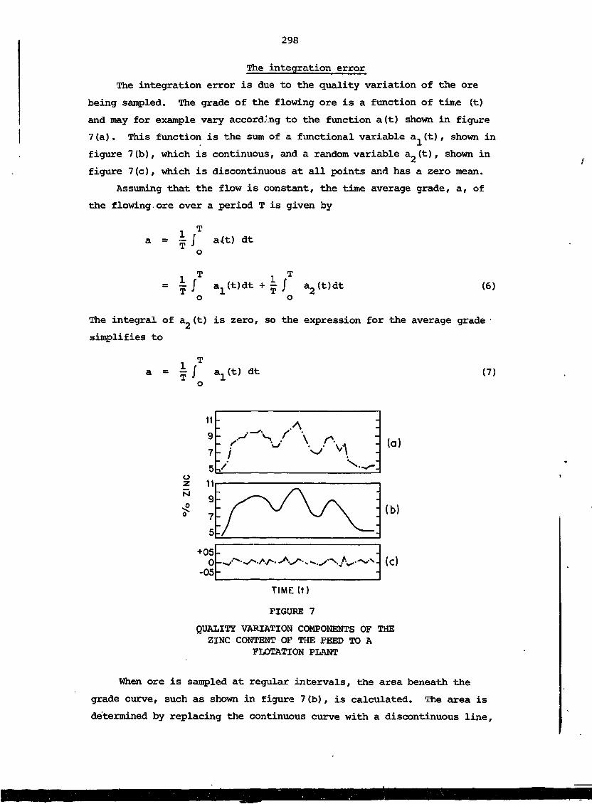
298
The integration error
The integration error is due to the quality variation of the ore
being sampled. The grade of the flowing ore is a function of time (t)
and may for example vary accordJ.ng to the function a(t) shown in figure
7(a). This function is the sum of a functional variable a.(t), shown in
figure 7(b), which is continuous, and a random variable a2(t), shown in
figure 7(c), which is discontinuous at all points and has a zero mean.
Assuming that the flow is constant, the time average grade, a, of
the flowing ore over a period T is given by
a = i / a<t) dt
a;L(t)dt + - J a2(t)dto o
(6)
The integral of a_(t) is zero, so the expression for the average grade •
simplifies to
ai(t) dt (7)
ozN
11
9
7
5
11
9
7
5
+050
-05
.A- f'~ I
.v\ (a)
(b)
(c)
TIME It)
FIGURE 7
QUALITY VARIATION COMPONENTS OF THEZINC CONTENT OF THE FEED TO A
FLOTATION PLANT
When ore is sampled at regular intervals, the area beneath the
grade curve, such as shown in figure 7(b), is calculated. The area is
determined by replacing the continuous curve with a discontinuous line,

299
the segments of which have equidistant, abscissae. In other words, an
integration error appears, with the estimated average grade (a ) beingE
given by
n
(8)
where n is the number of increments. It is intuitively evident that the
more variable the ore is, the larger this integration error will be.
The integration error also increases when the sampling interval is made
longer.
The quality variation (a ) of the ore is expressed as the standard
deviation of the variations in grade. It cannot be estimated a priori,
but can only be determined by a relatively long and costly series of
experiments involving periodic sampling of a number of consignments of
ore. Usual methods (e.g. ISO 3084: Iron Ores - Experimental Methods
for Evaluation of Quality Variation) often overestimate the true quality
variation, since variance components due to sample preparation, measure-
ment and sampling errors other than the integration error are included.
Although these other components can be subtracted if they are known, it
is usual to relate the measured quality variation to the total sampling
error (a ) by the equation
wn (9)
where n is the number of increments. Thus, when a is known, the numberw
of increments required to achieve a specified sampling precision is
readily calculated. Often, quality variation is classified simply as
large, medium or small.
Integration errors can also arise due to cyclic variations in
grade. Difficulties occur when the sampling time interval approaches
that of the cyclic variation. When the sampling interval is made
larger, it must not be a multiple of the period of the cyclic variation.
The risk of large integration errors decreases as the sampling interval
increases, because rarely does the period of cyclic variation remain
rigorously constant. Sometimes it may be necessary to use random
sampling to overcome difficulties caused by cyclic variations.

300
The rate of flow error
Variations in flow rate have the following consequences:
(i) Increments do not have the same mass,
(ii) Increments do not represent the same tonnage of ore.
(iii) The increment mass is not proportional to the tonnage represented.
Consequently, in the strictest sense, flowing ore should not be sampled
until its flow rate has been regulated in some way, although sampling at
constant mass intervals provides an alternative solution.
The operating error
It is often the operating errors that are the most serious, as they
may by themselves introduce very significant bias. There are a number
of steps that should be taken to reduce these errors. Firstly, rudi-
mentary installations should be avoided, because the resultant errors
far outweigh any savings in the capital costs of the equipment. Secondly,
only fully tested equipment should be used. Thirdly, sampling install-
ations and operations should be checked by a specialist. Because a
particular sampling installation or method is satisfactory at one mine,
it does not follow that it will work at another. Each ore and each
sampling problem have their own characteristics.
Another basic rule is to avoid any modification of the samples,
either by loss of material or by the introduction of foreign matter.
Routine sampling installations should be designed to permit rapid and
thorough cleaning, and should be operated by competent and careful
personnel who fully understand the economic implications of their role.
There are a number of other sources of operating error, which are
discussed below.
3.2 Design and Location of Primary Sampler
The primary sampler must be located where the entire consignment
can be sampled, but where biased samples cannot be taken.
There are a number of types of primary sampler, varying in mode of
movement and shape. The most widely accepted type is a primary sampler
installed at the discharge end of the conveyor belt, and constructed to
cut a complete cross-section of the trajectory of the ore stream when
taking an increment. A number of typical examples are illustrated in
figure 8.
The cutter must travel through the falling ore stream at a uniform
speed either in a plane perpendicular to the ore stream or along an arc
normal to the mean trajectory of the stream. The cutting aperture must
be at least three and preferably four times the maximum particle size to

301
be certain of collecting the largest fragments. This rule holds down to
3 mm particle size, below which a fixed cutting aperture of 10 mm should
be used. The cutter speed must not be too great, since its effect is to
reduce the effective aperture of the cutter (e.g. V
an aperture of 3d).max 1.2 m s~l for
Id Swing-orm type
FIGURE. 8
EXAMPLES OF CUTTER-CHUTE, CUTTER-BUCKET,AND SWING-ARM TYPE PRIMARY SAMPLERS
The primary sampler must be sufficiently robust to withstand the
mechanical wear and tear to which it is subjected. The capacity of
bucket-type cutters must be sufficient to hold the entire increment
without loss or overflow, whereas the cutter-chute type must have non-
restrictive flow characteristics. If a belt scraper is required to
remove ore adhering to the belt, the scraper must be located so that the
scraped material falls within the area traversed by the cutter. Under
dusty conditions, scoop-type cutters must be protected against alien
dust entering the sample while the cutter is stationary. The cutter
must move completely out of the stream after taking an increment.
3.3 Sampling Precision and Mass of Consignment
The desired sampling precision (a ) is determined on the basis ofseconomics, statistics and practicality.
The financial sampling precision E is determined approximately from
the formula
„ 100-M „E = W ———— PerW 100 s
(price of consignment) a (10)

302
where E is given in dollars per consignment, W is the consignment mass
in tonnes, M is the moisture content, an P is the price of dry ore in
dollars per tonne. If E is constant, e.g. $500 per consignment, and the
total price of the consignment is $100 000, the relative error is 0.5
per 'cent and the required number of increments (given by the equation
below) is nine, assuming that a =1.5 per cent.W
n w(11)
This error and number of increments may be satisfactory for small
consignments. However, for a large consignment, e.g. $1 000 000, the
value of a is 0.05 and the required number of increments becomes im-
practicably large (900 for a =1.5). Likewise, if a is constant, theW S
coefficient of variation of the price of the consignment is constant.
Usually, this is also unsatisfactory. Consequently, a compromise such
as that illustrated in figure 9 must be established. Once this has been
done, the sampling engineer can calculate the required number of incre-
ments for any consignment of ore of known quality variation a . Altem-Vr
atively, reference can be made to tables in the various international
sampling standards publications.
(/>.—
MASS OF CONSIGNMENT. W
FIGURE 9
SAMPLING PRECISION FOR VARIOUSCONSIGNMENT MASSES
3.4 Mass of Increments
The minimum mass of increments required to avoid sampling bias
depends upon the maximum particle size of the ore being sampled. These
masses are usually determined by experiment and can be found in the
appropriate international sampling standards. An example, taken from

303
ISO 3082: Iron Ores - Increment Sampling and Sample Preparation
Mechanical Method^ is presented below in table 1.
TABLE 1
MASS OF INCREMENTS FOR SAMPLING IRON ORE
Maximum Particle SizeICUtl
Over Up To and Including
150
100
50
20
10
250
150
100
50
20
10
Minimum Mass ofIndividual Increment
kg
190
40
12
4
0.8
0.3
Minimum AverageMass of Increment
kg
320
70
20
6.5
1.3
0.5
The average mass of increments (M kg) taken by a cutter-type primary
sampler can be calculated from the formula
M CA3.6V (12)
where C is the average flow rate in tonnes per hour/ A is the cutting
aperture of the primary sampler in metres, and V is the cutter speed in
metres per second.
3.5 Mass-basis Sampling
In mass-basis sampling, the required number of increments are taken
at fixed tonnage intervals, T, given by the relationship
n (13)
where W is the mass of the consignment in tonnes, and n is the number of
increments determined from equation (11).
The increments must be taken in such a manner that they have almost
uniform mass, e.g. by using a variable speed cutter. A coefficient of
variation of 20 per cent is permitted in most applications.
3.6 Time-basis Sampling
In time-basis sampling, the increments are taken at fixed time
intervals, t, given by the relationship
60wC nm
(14)

304
where C is the maximum flow rate of the conveyor in tonnes per hour,mThe mass of each increment must be proportional to the flow rate of
the ore stream at the time of sampling. For this purpose a fixed speed
cutter is required. The relative masses of the individual increments or
sub-samples must be preserved throughout the sample preparation stages
to obtain the correct weighted mean for the final analysis.
3.7 Sample Division and Sample Preparation
Sample -division and sample preparation are the successive division
and crushing steps that enable a sample weighing many kilograms to be
reduced to a representative small sample of several hundred grams for
chemical analysis.
There are a number of different methods of sample division.. These
may be either manual or mechanical. In all cases there is a minimum
mass of divided sample, which depends on the ore type and on its present
maximum particle size. Table 2 gives examples of minimum masses of
divided samples taken from ISO 4296/2: Manganese Ores - Preparation of
Samples*
TABLE 2
MINIMUM MASS OF SAMPLE AFTER DIVISION
Maximum Particle Size,mm
50
22.4
15
10
5
3
1
0.5
0.1
Minimum Mass of Sample,kg
250
45
25
10
3
2
1
0.4
0.2
Methods of manual division include increment division, division
by riffling, and division by coning and quartering. Of these, the
coning and quartering method is the least satisfactory. The increment
division method consists of spreading the sample out into a uniform flat
rectangle on a smooth flat plate. Markings are made on the surface of
the sample dividing it into 20 equal parts. A shovelful of ore is taken
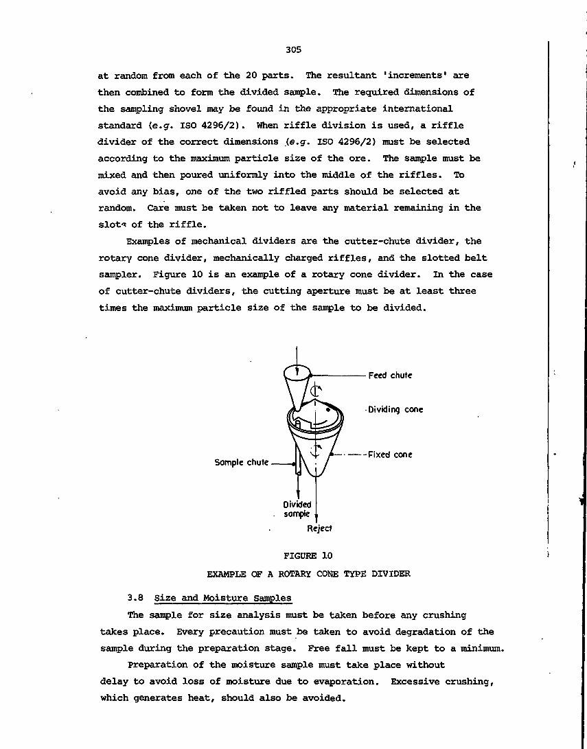
305
at random from each of the 20 parts. The resultant 'increments' are
then combined to form the divided sample. The required dimensions of
the sampling shovel may be found in the appropriate international
standard (e.g. ISO 4296/2). When riffle division is used, a riffle
divider of the correct dimensions .(e.g. ISO 4296/2) must be selected
according to the maximum particle size of the ore. The sample must be
mixed and then poured uniformly into the middle of the riffles. To
avoid any bias, one of the two riffled parts should be selected at
random. Care must be taken not to leave any material remaining in the
slot-* of the riffle.
Examples of mechanical dividers are the cutter-chute divider, the
rotary cone divider, mechanically charged riffles, and the slotted belt
sampler. Figure 10 is an example of a rotary cone divider. In the case
of cutter-chute dividers, the cutting aperture must be at least three
times the maximum particle size of the sample to be divided.
Sample chute
Feed chute
Dividing cone
Fixed cone
Dividedsample
Reject
FIGURE 10
EXAMPLE OF A ROTARY CONE TYPE DIVIDER
3.8 Size and Moisture Samples
The sample for size analysis must be taken before any crushing
takes place. Every precaution must be taken to avoid degradation of the
sample during the preparation stage. Free fall must be kept to a minimum.
Preparation of the moisture sample must take place without
delay to avoid loss of moisture due to evaporation. Excessive crushing,
which generates heat, should also be avoided.

306
4. SAMPLING FROM STOCKPILES
The in situ sampling of ore in stc.kpiles and shipholds should be
avoided at all cost, because the equi-probable sampling model is un-
likely to be applicable. For example, it is virtually impossible to
sample material near the bottom of a large stockpile. It is always
advisable to sample a batch of ore when it is in motion. When this is
impossible, sampling probes may be used. These probes are essentially
hollow pipes of appropriate diameter (considering the particle size of
the ore to be sampled), which are thrust into the ore. This method is
satisfactory only if the full core can be withdrawn without loss of
sample material.
5. SAMPLING.OF SLURRIES
The fundamental sampling considerations for slurries are, in
principle, t e same as those for sampling crushed ore on conveyor belts.
It is always preferable to sample the slurry where it is flowing in a
continuous stream. When the diameter of the largest particles in the
stream is less than 3 mm, the cutting aperture of the primary sampler
should be 10 mm. Sampling by dipping into the slurry is usually un-
satisfactory, because size segregation will undoubtedly be present.
6. BIBLIOGRAPHY
AIMM [1976] - Proc. Symp. Sampling Practices in the Mineral Industries.
Australasian Institute of Mining and Metallurgy, September.
Blaskett, K.S. [1980] - The Sampling of Slurries. Proc. Symp. on
Sampling in the Process Industries, Adelaide, August.
David, M. [1970] - Geostatistical Ore Estimation - A Step-by-step Case
Study. Proc. 9th Int. Symp. for Decision Making in the Mineral
Industry, CIM (Can. Min. Metall.) Bull., Special Volume No. 12,
p. 185.
Gy, P.M. [1972/1973] - The Sampling of Broken Ores; A Review of
Principles and Practice. In Geological, Mining and Metallurgical
Sampling. Proc. Institution of Mining and Metallurgy Meetings
held in London on January 1972, September 1972 and July 1973.
Gy, P.M. [1979] - Sampling of Particulate Materials - Theory and
Practice. In Developments din Geomathematics, Vol. 4. Elsevier
Scientific Publishing Company, New York.
Gy, P.M. & Martin, L. [1978] - Unbiased Sampling from a Falling Stream
of Particulate Material. Int. J. Miner. Process., 5:297.

307
Ishikawa, K. [1972/1973] - Establishment and Control of the Sampling
Procedure for Bulk Materials. In Geological, Mining and Metallurgical
Sampling. Proc. Institution of Mining and Metallurgy Meetings held
in London on January 1972, September 1972 and July 1973, p. 206.
Matheron, G. [1963] - Traite" de Ge"ostatistique Applique*e - Tome II:
Le Krigeage. Editions Technip, Paris.
Royle, A.G. [1979] - Why Geostatistics? Eng. Min. J., 180:92.

309
CHAPTER 7
FIELD MEASUREMENTS IN BOREHOLES
A series of lectures
J. AylmerP.L. EislerP. HuppertP.J. Mathew

311
PART A
NATURAL GAMMA SPECTROSCOPY FOR BOREHOLE LOGGING
by
J. Aylmer

313
1. INTRODUCTION
The decay series of thorium and uranium is well established (table
1). The disintegration of the natural radioelements is accompanied by
a, g and Y emissions, the latter having energies characteristic of the
particular isotopic decay. Using established technology, these y-xays
can be readily detected.
The spectroscopy technique is now widely used in the mining industry
as an aid to geological mapping, for surface investigations, and for
down-hole investigation of stratigraphy and ore grade. The straight-
forward concept of natural y spectroscopy makes it possible for the
instrumentation to be simple to operate, yet have a sensitivity capable
of providing reliable data under field conditions.
2. THEORETICAL CONSIDERATIONS
2.1 Abundance in Rocks
All rocks and soils (as distinct from ores) contain a great number
of radioactive elements that emit y radiation. The three main sources
of natural y-rays are:
(a) Potassium-40, which is 0.012 per cent of total potassium, and
emits a single y~ray of 1.46 MeV.
(b) Decay products in the uranium-238 and uranium-235 decay
series.
(c) Decay products in the thorium-232 series.
Table 2 lists the average abundance of natural radioelements in
various types of rock. Limestones and dolomite and non-shaly sandstones
have even less radioactivity than indicated in the table, whereas bit-
uminous coals, rocksalt, gypsum and hematite have the lowest activity of
all.
In terms of counts s"1 kg""1 of rock (measured with a 50 mm x 50 mm
scintillation counter having a cylindrical geometry), the natural
radioactivities referred to have approximate values:
Total activity
(counts s""1 kg"1)
Shales Sandstone Hematite and Bituminous Coal
0.2
These values cover a wide spread of concentrations and refer to a
statistical distribution of values about a mean. The values are typical
for deposits that are potassium deficient. When potassium-rich clays
(illites and feldspars, etc.) are present, this may increase the total
activity by about 50 per cent.

Thorium Mrin (4n) Uranium-Radium serial (On » 2)
TABLE 1
DECAY SCHEMES FOR THE NATURALOCCURRING RADIOACTIVE NUCLIDES
IN THE 4n, 4n + 2 AND 4n + 3 SERIES

315
TABLE 2
AVERAGE ABUNDANCE OF NATURAL RADIOELEMENTS
Rock Type
Magmatic,
acid
intermediate
basic
ultrabasic
'Common shales'
U Th
tppm)
5
2
1
0.6
4
20
8
4
2
12
•»0K
3.3
2
2
0.5
2
2.2 Instrumentation
The development of highly sensitive detectors allows quantitative
analysis of natural y radiation. It will be assumed here that
Nal(Tl) scintillation crystals are being used. These detectors have a
very wide acceptance because of their high efficiency, particularly in
the low energy region of the spectrum. A comparison of detector effic-
iencies is given in figure 1.
Typical instrumentation for Y~raY logging is shown in schematic
form in figure 2. The spectrum-analysing equipment can be as simple (or
complex) as desired. The information obtained can range from a single
total count number on a printer or digital display, to a full spectral
trace on an X-Y plotter. Typical spectra for the thorium and uranium
decay series are shown in figure 3.
The detector crystals are cylindrical and hence compatible with the
probe, and can vary in size from 20 mm diameter by 20 mm length for
qualitative stratigraphic work, to 50 mm by 50 mm for quantitative
interpretation.
The down-hole equipment shown in figure 2 is all that is required
unless there is a need for temperature compensation, and/or optimum
spectral resolution. For very deep holes, such as those used in the oil
industry, the temperature may rise to 150°C and the pressure to 100 000
kPa. Probes used under these conditions are very specialised, and
qualitative comparisons may be the only data obtainable.
2.3 Spectrum Interpretation
Although a large number of energy peaks appear in the natural y
spectrum, the photons of energy 1.765 (214Bi), 2.615 (208T1), and 1.461
MeV (£*°K) are accepted as being the most suitable for uranium, thorium

316
3.4.5 1,20-020-r 1-0
0-OI6-- 08|-ogo
zp 0-008-1- 0-4oaiuJ 0-004-1- 0-2o
0-L0 0-4 0-8 1-2 1-6 2-0 2-4 2-8
. ENERGY(MeV)
FIGURE 1
EFFICIENCY CURVES OF GAMMA DETECTORS(1) Scintillation counter Nal(Tl), height of
crystal 50 mm; (2) scintillation counter Nal(Tl),height of crystal 20 mm; (3) GM counter, W cathode;
(4) GM counter, Cu cathode; (5) GM counter, steel cathode.
••
. Down- hole electronics
Amplifierstabiliser
Single channelanalyser
Rate-meter
IChart recorder
•Nal (Tl) detector crystaland photo multiplier tube
Counter timer
ILine printer
FIGURE 2
SCHEMATIC REPRESENTATION OF THE LOGGINGPROBE, SHOWING ALSO THE PROBABLE DATA
ANALYSING INSTRUMENTATION

317
< CD
05
ENERGY (MeV)
1O 15 2O 25
4O 8O 12O 16OCHANNEL NUMBER
2OO
FIGURE 3a
THE SPECTRUM FROM URANIUM AND ITSDECAY PRODUCTS, WITH THE MAJOR PEAKS INDICATED
<tfflU
O-5
ENERGY(MeV)
15 2O 2 5 30
4O 8O 12O 16OCHANNEL NUMBER
20O 24O 28O
FIGURE 3b
THE SPECTRUM FROM THORIUM AND ITSDECAY PRODUCTS, WITH THE MAJOR PEAKS INDICATED

318
and potassium measurement respectively.
Using a suitable pulse height analysis system, it is possible to
provide a four-channel facility to determine the total activity and the
contribution made by the individual radionuclides. The spectral band
energies usually selected for the analysis are as follows:
Radionuclide 40K U(21lfBi) Th(208Tl) TotalActivity
Energy Range (MeV) 1.36-1.56 1.66-1.81 2.51-2.71 0.4-3.0
Although the above peaks are specific, and not subject to pronounced
interfere.ve from immediately adjacent peaks, their Compton tails overlap
and background must be subtracted. This is achieved by means of strip-
ping ratios a, 3 and y» resulting in the following expressions for
corrected Th, U and K counts:
NTh - NTl-BThcorr.
""corr. = "» - B» ' "V
\ - "K - BK - (3NTh - YVcorr.
where B_, B and B are backgrounds.j.n, u &
2.4 Detector Response
Stationary detector
There are a number of factors to be considered for a stationary
detector in a borehole:
The detector has a higher probability of intersecting and
detecting radiation from disintegrations near the sensitive
element than from those further away.
There is a solid angle effect, 1/r2 when the matrix is not
infinite.
There is an exponential term for the probability of absorption
between source and detector.
Some complex behaviour occurs close to the detector, par-
ticularly in relation to backscattered radiation, but it is
not significant in the overall picture.
Looking from the detector outwards, spheres of investigation can be
defined in which given percentages of the detected counts originate.
These can be 50, 70 or n per cent, where n < 100 per cent for any

319
'/2 maximumdeflection
Barren formation
Radioactive formation
'Approximatedetectorresponse
Barren formation
(a)
ApproximateV /detectorN^response
Barren formation
Radioactive formation
Barren formation
(b)FIGURE 4
DIAGRAMATIC REPRESENTATION OF THE STRATAEFFECT ON THE RESPONSE OF THE DETECTOR
TO ACTIVE LAYERSThe response refers to the sphere of sensitivity of the
detector - radius R. (a) For a layer of infinite thickness(i.e. greater than 2R), the response will be the maximum
possible for the relative activity of the material.(b) For layers less than 2R in thickness, the steady
state count rate appropriate to the activity of the materialis never reached.

320
homogeneous medium. A common value is n = 99 per cent; the probability
of detecting radiation originating outside this sphere can be considered
negligible. The volume within the sphere (of radius R) is referred to
as the sensitive volume of the detector.
Any bed thicker than 2R, and extending further than R radially from
the hole, is considered to be infinite. Assuming that the sensitive
volume remains constant in different media, the count rate is proport-
ional to the concentration of the source element, or the parent in the
case of a radioactive series in equilibrium.
Moving detector
The shape of the sensitive volume changes under dynamic conditions;
the faster the detector moves, the more elongated the sensitive volume
becomes. In theory, this volume retains cylindrical symmetry, but in
practice the hole and the probe introduce minor departures from this
condition.
2.5 Strata Effects
After the stratigraphic sequence has been classified, the next step
is to quantify the thickness and grade of each zone. As the detector
approaches a radioactive zone, the sphere of influence permits detection
before becoming coincident with the zone. If the stratum is infinitely
thick (i.e., has a vertical dimension greater than twice the radius of
the sphere of influence of the crystal), the maximum response will be .
given as the detector passes across the face. Such an arrangement
should be made for calibration holes, but this situation is not always
encountered in practice. In many cases, the stratum is less than 2R in
thickness. The detector will then be influenced by strata on both
sides, and the maximum response will not be recorded. The effects of
stratum boundaries, and detector behaviour with zones of different
thickness, are shown schematically in figures 4a and 4b.
The response obtained from each stratum can be traced on a chart
recorder. The area (A) of a recorded anomaly, the true thickness (h) of
the radioactive layer, and the recorded intensity (i ) of an infinitely00
thick stratum can be related as follows:
A = h x im
which can be expressed as
A a hQ or A = ChGy
where Q = grams of radioactive material per gram of rock,
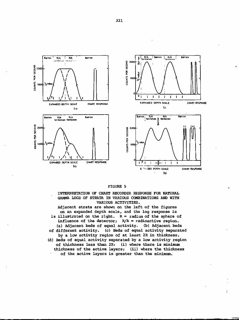
321
I Borren ' R/A i Barren
§ 2000
1000 Jfc "Okie.
I c | R/A ! Barren ! R/A BarrenI f <ormo*ion ' *or-mc*«p«
I I I I I I I I
EXPANDED DEPTH SCALE
ba
CHART RESPONSE EXPANDED DEPTH SCALE
5c
CHART RESPONSE
2000-
fiz 1000
Barren R/A R/Aformation formation
Barren
_'/2vo1ue
EXPANDED DEPTH SCALE
5bCHART RESPONSE I -R -I I -ISI- I I I
E "*-.OED OTTH SCALE
5dCHART RESPONSE
FIGURE 5
INTERPRETATION OF CHART RECORDER RESPONSE FOR NATURALGAMMA LOGS OF STRATA IN VARIOUS COMBINATIONS AND WITH
VARIOUS ACTIVITIES.Adjacent strata are shown on the left of the figureson an expanded depth scale, and the log response is
is illustrated on the right. R = radius of the sphere ofinfluence of the detector; R/A = radioactive region,(a) Adjacent beds of equal activity, (b) Adjacent beds
of different activity, (c) Beds of equal activity separatedby a low activity region of at least 2R in thickness,
(d) Beds of equal activity separated by a low activity regionof thickness less than 2R: (i) where there is minimumthickness of the active layers; (ii) where the thickness
of the active layers is greater than the minimum.

322
Gy = average weight per cent of, e.g., U,O_, K9O, etc., and
C is an equipment calibration constant.
Estimates using the above expression can be made from chart re-
corder responses. Figures 5a to 5d show the type of response, and the
interpretation which can be applied.
Because of boundary ar.3 instrvroental effects, the method is most
suitable for relatively thick strata, fast-reacting equipment and ade-
quate counting statistics. This is affected not only by the mean count,
but also by the speed of logging.
In multistratified deposits, logging rates of 3 to 6 m min"* are
suitable for qualitative work, and 1.5 to 3 m min"1 for quantitative
surveys. The speed of logging should be adjusted according to the
number of stratiyrdphic changes down the borehole.
2.6 Matrix Effects
The borehole
The ideal logging situation is that the hole be dry, have a di-
ameter close to that of the calibration hole, and not be cased (lined
with a metal tube). Under these conditions, and if the strata are
relatively thick, the response is independent of borehole diameter.
If the holes are full, or partly full of water/ drilling mud, etc.,
or are cased, the probe must be centralised and the necessary correction
factors applied. These factors, which can be complex, have been thor-
oughly investigated and reported in various publications (e.g., see
Rhodes and Mott 1966).
The surrounding rock
For a dry hole, in rock containing Q g of radioactive material per
gram, the intensity, I, of unscattered y radiation is given by
I = 4ir k p/y x Q
where p/y is the reciprocal of the mass attenuation coefficient for
radiation of energy used to assess Q. If the atomic number (Z) of the
surrounding rock is not too large, the expression reduces to:
I = const, x Q
i.e. the intensity of response is directly related'.to the concentration
of the radionuclides.
Experimental results, however, show that the response of scintill-
ation detectors to y radiation varies according to the size of detector

323
and the energy discrimination threshold. Low energy y-rays (< 0.4 MeV)
are increasingly absorbed as the effective atomic number of the surround-
ing rock increases. The intensity in this low energy region will depend
on the concentration of the radionuclides, and on the rock matrix. To
avoid this problem, it is desirable to discriminate (instrumentally)
against y-rays with energies less than 0.4 MeV. This applies when
investigating individual radionuclides, and particularly for .total
natural y spectroscopy.
2.7 The Natural Radioactive Background
The values quoted in section 2.1 for activities (counts s"1 kg"1)
are the above 'background1 results in a lead-shielded enclosure lined
with cadmium and copper to suppress lead X-rays.
The borehole is less susceptible to background influences than
surface or airborne surveys; however, the term 'background1 in a geo-
scientific context should be restricted solely to radiation which does
not originate from- the active strata. This would include cosmic rays,
atmospheric radioactivity and the radioactivity of the counting system,
particularly the detector. Any unexpectedly high radioactivity which
cannot be explained in geochemical terms should be analysed by y spectro-
metry to determine whether short-lived fallout products are present.
2.8 Calibration of the Logging System
If possible, instrumental and probe calibrations should be carried
out in the laboratory and again in situ. A series of laboratory radio-
metric counting standards should be designated as the primary standards
for the entire calibrating system. Nationally certified and preferably
internationally inter-calibrated standard samples should be chosen,
e.g./ laboratory samples of uranium and thorium materials analysed by
the International Atomic Energy Agency (IAEA). These should be used for
carefully controlled instrumental checks.
Secondary calibration facilities, in the form of model holes,
should be available. A few carefully designed and constructed models
can provide all the requirements for standard conditions of calibration.
Models can usually be constructed using concrete (with additives of
ore), allowing close control over concentration, density, thickness of
ore zone, hole diameter and homogeneity. Figure 6 illustrates the basic
design for a calibration model with the radioactive zone being of a
thickness to ensure maximum detector response. It is usually impracti-
cable to transport these models to exploration sites. The system, with
reference to the. primary and secondary standards, may be calibrated in
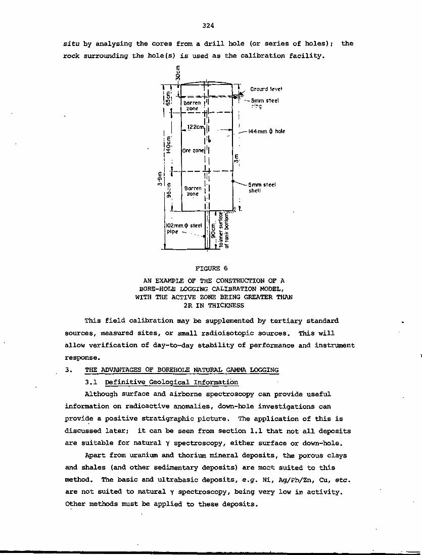
324
situ by analysing the cores from a drill hole (or series of holes); the
rock surrounding the hole(s) is used as the calibration facility.
1 1
1: E0o
E
uu^en
Eu
-5-4-1
—
i
™«Borren
gl -B
'1
-— iij— •_>122cmi| „
I "
iliOre zone|'|
t~~1Borrenzone
102mm $ steelpipe -. .
j
(
i
'. x Grourd level
P --5mm steel
!
1
. — 144 mm $ hole
Ewi
^~^-5mm steelshell
!{Te =B5S|1
FIGURE 6
AN EXAMPLE OF THE CONSTRUCTION OF ABORE-HOLE LOGGING CALIBRATION MODEL,WITH THE ACTIVE ZONE BEING GREATER THAN
2R IN THICKNESS
This field calibration may be supplemented by tertiary standard
sources, measured sites, or small radioisotopic sources. This will
allow verification of day-to-day stability of performance and instrument
response.
3. THE ADVANTAGES OF BOREHOLE NATURAL GAMMA LOGGING
3.1 Definitive Geological Information
Although surface and airborne spectroscopy can provide useful
information on radioactive anomalies, down-hole investigations can
provide a positive stratigraphic picture. The application of this is
discussed later; it can be seen from section 1.1 that not all deposits
are suitable for natural y spectroscopy, either surface or down-hole.
Apart from uranium and thorium mineral deposits, the porous clays
and shales (and other sedimentary deposits) are moct suited to this
method. The basic and ultrabasic deposits, e.g. Ni, Ag/Pb/Zn, Cu, etc.
are not suited to natural y spectroscopy, being very low in activity.
Other methods must be applied to these deposits.

325
3.2 The Finite Penetration of Gamma-rays
Gamma-rays are electromagnetic radiations, not electrically
charged, and of very short wavelength. Compared to a and & radiation
penetration is several orders of magnitude greater through rock. How-
ever, figure 7 illustrates that there are restrictions on the degree of
penetration of, e.g. uranium radiation. A rock cover of 20 usa reduces
the Y~raY intensity to 64 per cent and, with a cover of 0.5 m, conven-
tional surface equipment would not detect the anomaly.
lOOr
9oi
8C)|
7C
100 300 500 700THICKNESS OF COVERING ROCK(mm)
FIGURE 7
PENETRATION OF GAMMA RADIATION FROM ANINFINITE URANIUM ORE DEPOSIT WHICH IS
COVERED BY A ROCK LAYER
Borehole logging is thus essential in such a case, to establish the
presence of the deposit and to provide stratigraphic details.
4. THE DISEQUILIBRIUM FACTOR
This is a geochemical factor, and has an important bearing on the
interpretation of spectrometric results. In most exploration and mine
evaluation work, it is assumed that the radionuclides are in equilibrium
with their daughter products. There are a number of ways in which the
decay chains (particularly that of 238u) may be broken.
(a) If a uranium-rich deposit is subject to leaching by neutral or
slightly alkaline ground waters, the soluble uranium is trans-
ferred in solution to a new site. The daughter products
remain, and on spectral investigation will give the character-
istic 1.76 MeV (214Bi) peak which indicates the presence of
uranium. This will be inconsistent with what is actually
present.

326
Alternatively, the uranium may have been deposited in
recent geological times and will not be in equilibrium with
its daughter products. The spectrum of recently-prepared U0_
in figure 8 illustrates that the spectral investigation of a
new deposit will not detect the 1.76 MeV peak, even though
uranium is actually present.
- '"Th-i-K X- rays
- PbIK X-ray
0-2 04 1-4 t-6 1-8 2-00-6 08 VO 1-2ENERGY(MeV)
FIGURE 8
FRESHLY PREPARED URANIUM DIOXIDE, WHICHHAS NOT YET GROWN UP APPRECIABLE ACTIVITY
FROM RADIUM-226 AND DAUGHTERS.The spectrum was taken with a 76 x 76 mm
Nal(Tl) scintillation detector.
(b) Radon (222Rn) is a gas that can escape easily to the atmos-
phere, and this is sometimes detected by surface or airborne
investigation. The loss of radon causes the most severe
disequilibrium, and causes problems in prospecting, and the
interpretation of information. It can be seen that it breaks
the chain before the formation of 211fBi, resulting in a lower
spectral response for the uranium concentration.
These disequilibrium problems also apply to shales, etc. which have
trapped the radionuclides (e.g. 238U). Careful spectral analysis would
be required to resolve these problems and would need to be accompanied
by chemical analysis. High resolution germanium detectors are now being
used to solve the problem.

w10o
Natural gamma log
FIGURE 9
SCHEMATIC REPRESENTATION OF ACTIVE STRATAWITHIN A DEPOSIT BEING INTERSECTED BY A
BOREHOLE, AND THE RESULTANT NATURAL GAMMA LOG.

328
5. APPLICATIONS OF NATURAL GAMMA LOGGING
5.1 Stratigraphic Interpretation
This application applies primarily to deposits of the sedimentary
type, where information is required on the individual stratum. Using
data from the natural y log, the extent of such deposits can be assessed.
A simple logging application is shown diagrammatically in figure 9.
The entrapment of radioactive minerals by porous shales and clays
provides the oil industry with a means of establishing the presence and
Stratigraphic location of these shales. Figure 13a shows a chart re-
corder trace of a typical log of total activity. The presence and
location of an anomaly is noted, and can be combined with similar in-
formation from other holes to give a three-dimensional geological map.
Sedimentary iron ore deposits
The sedimentary iron ore deposits of Western Australia are char-
acterised by macrobands of high-grade hematite and shale. The shale
contains radionuclides which are readily detected by scintillation
crystals. By logging for total activity, the stratigraphy of the ore-
body is delineated; examples are shown in figure 10.
The procedure of appraisal is the opposite to that for oil well
logging, in that the material being sought (hematite) has negligible
activity, and the shale containing the natural activity is low-grade
waste.
Patterns of deposition have been established over the extent of a
mining lease in Western Australia. It is shown in figure 11 that par-
ticular bands appear in the same relative position in the strata.
Coal deposits
It was noted in section 2.1 that bituminous coal is very low in
activity. The stratigraphy therefore can be mapped by detecting activ-
ity in the ash (shales, etc.) layers. Figure 12 shows an example of a
natural y 1°9 °f a coal deposit.
The danger of using this log alone to classify bands of coal and
ash is that sandstone is also low in activity and, unless found in con-
junction with shale, cannot be distinguished from coal. Sandstones with
some shale have an observable activity but cannot be distinguished from
carbonaceous shales. Results of such a log must be treated with caution
unless supplemented by other information, e.g. a density log.
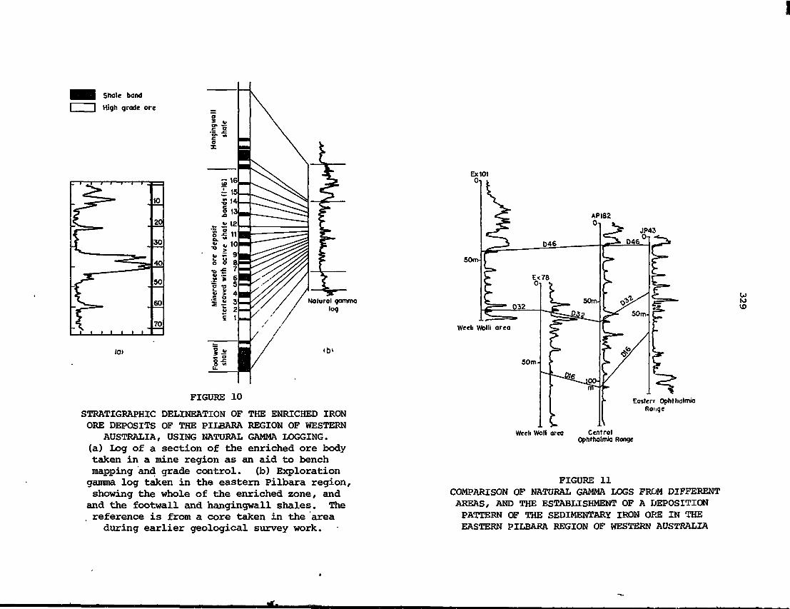
Shale band
High grade ore
Natural gammalog
fa>
FIGURE 10
STRATIGRAPHIC DELINEATION OF THE ENRICHED IRONORE DEPOSITS OF THE PILBARA REGION OF WESTERN
AUSTRALIA, USING NATURAL GAMMA LOGGING,(a) Log of a section of the enriched ore bodytaken in a mine region as an aid to benchmapping and grade control, (b) Explorationgamma log taken in the eastern Pilbara region,showing the whole of the enriched zone, andand the footwall and hangingwall shales. The. reference is from a core taken in the area
during earlier geological survey work.
JP43
50m
totoVO
Weed Wolli area
Eosterr OphthalmiaRange
Weed WolG area CentralOphthalmia Range
FIGURE 11COMPARISON OF NATURAL GAMMA LOGS FROM DIFFERENTAREAS, AND THE ESTABLISHMENT OF A DEPOSITIONPATTERN OF THE SEDIMENTARY IRON ORE IN THEEASTERN PILBARA REGION OF WESTERN AUSTRALIA

W4OO-
~! 2OO-
3 o-i
Shale bandsII
Shale bandsI II I I I
I Iu>OJo
59^ 9399 125
IshalesSSJ
222 248 2561/2Sandstones
FT
FIGURE 12
NATURAL GAMMA LOG OF A QUEENSLAND COALDEPOSIT, INDICATING THE BANDS OF ASH
(SHALES etc.) WITHIN THE COAL
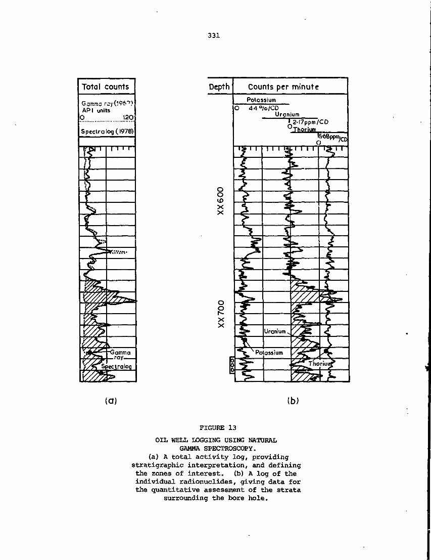
331
Total counts
API unitsO 12O
Spectra log (1978)
™ I l i «
j ammo.ray—
eclraloq
Counts per minute
0 44 °/o/CDUranium
(a) (b)
FIGURE 13
OIL WELL LOGGING USING NATURALGAMMA SPECTROSCOPY.
(a) A total activity log, providingstratigraphic interpretation, and definingthe zones of interest, (b) A log of theindividual radionuclides, giving data forthe quantitative assessment of the strata
surrounding the bore hole.
332
5.2 Quantitative Aspects of Natural Gamma Logging
Having established the presence of radioactive anomalies by using a
qualitative scan, more detailed down-hole work can be undertaken. This
may include a static spectrum of particular regions, a log to determine
individual radionuclides, or a detailed assessment of the width and
grade of the various zones around the borehole.
Oil well logging
Figure 13b illustrates that suitable analysis equipment permits a
log of individual radioelements. The intensity of the peaks of Th, U
and K displayed on the chart recorder would also be available as num-
erical data. This information can be used individually or in combin-
ation to aid the search for oil-rich shales.
Figures 14a and 14b show the spectral data which correlate with
organic carbon. In subsequent logging, a direct readout of U:K would
give a direct log of the product sought.
Iron ore deposits
Because the sought after material (hematite) has negligible activ-
ity, the problem is slightly more complex. The total and individual
radionuclide activities of the shale bands are grouped around mean
values, and cannot be used to classify individual bands.
Spectral examination revealed the presence of potassium ( K) in
the footwall and hanging wall shales. Figures 15a and 15b give the
spectral comparison between orebody and footwall shales, indicating that
a potassium log would pinpoint the extent of the orebody. The ferr-
uginous orebody shales of these deposits are simple shale/hematite
mixtures. The width and activity of these shale bands can be esta-
blished but there seemed to be no simple way to relate grade to the
natural activity.
However, in a series of static tests, hematite was added to non-
ferruginous shales. Figure 16 shows that for orebody shales, with a
shale content of below 50 per cent, a linear relationship exists between
total activity and shale content. This shale content can be related to
wt % Fe as shown in figure 17.
For the Western Australian deposits, it was possible to log natural
Y activity, and from this estimate the mean grade of iron in dry bore-
holes traversing layers of hematite and shale. The data were subjected
to a regression analysis. With the resultant linear expression relating
activity and ore grade, it was possible, for a group of blast holes and
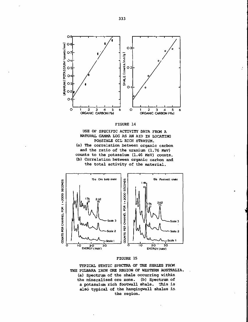
333
O-3
O-1
1 2 3 4 5ORGANIC CARBON (°/o)
1 2 3 4 5ORGANIC CARBON (%>)
FIGURE 14
USE OF SPECIFIC ACTIVITY DATA FROM ANATURAL GAMMA LOG AS AN AID IN LOCATING
POSSIBLE OIL RICH STRATUM.(a) The correlation between organic carbonand the ratio of the uranium (1.76 MeV)
counts to the potassium (1.46 MeV) counts.(b) Correlation between organic carbon and
the total activity of the material.
15 a Ore body shale
Scale 3
Scale 2
Scale!
VO 2-O 3-OENERGY (MeV)
ISb Footwall shale
Scale 3
Scale 2
Scale 1
1O 20 30ENERGY (MeV)
FIGURE 15
TYPICAL STATIC SPECTRA OF THE SHALES FROMTHE PILBARA IRON ORE REGION OF WESTERN AUSTRALIA.
(a) Spectrum of the shale occurring withinthe mineralised ore zone, (b) Spectrum ofa potassium rich footwall shale. This isalso typical of the hangingwall shales in
the region.

334
0 10 20 30 40 50 60 70 8 90% SHALE
FIGURE 16
NATURAL GAMMA-RAY RESPONSE ABOVE 400 keVIN SYNTHETIC MIXTURES OP HEMATITE AND SHALE.
20 40 60 80SHALE CALCULATED BY DIFFERENCE
EX Fc203
FIGURE 17
CHEMICAL ASSAYS FOR THE SHALE (KAOLINITE)TAKEN FROM A MINE AREA IN THE PILBARA,CONFIRMING SIMPLE SHALE/HEMATITE MIXTURES
IN THE MINERALISED ZONE.This simple system allows grade
estimation by natural gamma logging.
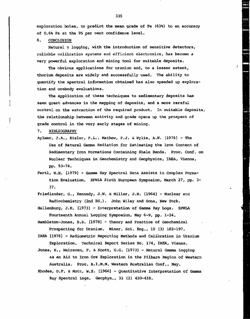
335
exploration holes, to predict the mean grade of Fe (63%) to an accuracy
of 0.6% Fe at the 95 per cent confidence level.
6. CONCLUSION
Natural y logging, with the introduction of sensitive detectors,
reliable calibration systems and efficient electronics, has become a
very powerful exploration and mining tool for suitable deposits.
The obvious applications for uranium and, to a lesser extent,
thorium deposits are widely and successfully used. The ability to
quantify the spectral information obtained has also speeded up explora-
tion and orebody evaluations.
The application of these techniques to sedimentary deposits has
seen great advances in the mapping of deposits, and a more careful
control on the extraction of the required product. In suitable deposits,
the relationship between activity and grade opens up the prospect of
grade control in the very early stages of mining.
7. BIBLIOGRAPHY
Aylmer, J.A., Eisler, P.L., Mathew, P.J. & Wylie, A.W. [1976] - The
Use of Natural Gamma Radiation for Estimating the Iron Content of
Sedimentary Iron Formations Containing Shale Bands. Proc. Conf. on
Nuclear Techniques in Geochemistry and Geophysics, IAEA, Vienna,
pp. 53-74.
Fertl, W.H. [1979] - Gamma Ray Spectral Data Assists in Complex Forma-
tion Evaluation. SPWLA Sixth European Symposium, March 27, pp. 3-
37.
Friedlander, G., Kennedy, J.W. & Miller, J.M. [1964] - Nuclear and
Radiochemistry (2nd Ed.). John Wiley and Sons, New York.
Hallenburg, J.K. [1973] - Interpretation of Gamma Ray Logs. SPWLA
Fourteenth Annual Logging Symposium, May 6-9, pp. 1-24.
Hambleton-Jones, B.B. [1978] - Theory and Practice of Geochemical
Prospecting for Uranium. Miner. Sci. Eng., 10 (3) 182-197.
IAEA [1976] - Radiometric Reporting Methods and Calibration in Uranium
Exploration. Technical Report Series No. 174, IAEA, Vienna.
Jones, H., Walraven, F. & Knott, G.G. [1973] - Natural Gamma Logging
as an Aid to Iron Ore Exploration in the Pilbara Region of Western
Australia. Proc. A.I.M.M. Western Australian Conf., May.
Rhodes, D.F. & Mott, W.E. [1966] - Quantitative Interpretation of Gamma
Ray Spectral Logs. Geophys., 31 (2) 410-418.

336
APPENDIX A
TECHNICAL INFORMATION REQUIRED FOR REPORTING ON
BOREHOLE RADIOACTIVE LOGGING
The following data should be recorded on the log. The type of
information which should be included when reporting logging data is
commonly printed on a log heading, attached to the original and copies
of logs. Not uncommonly, several types of log are obtained simultan-
eously; analog (strip chart) records are generally aligned in parallel
and each of the logs is positioned to a common 'collar', or ground zero
depth. The y log heading should include:
(a) hole identification, coordinates and elevation of collar if
known, drilled depth and logged depth;
(b) probe identification number, calibration factor, detector data
such as crystal size and type, surface density (g cnf2), o.d.
(outside diameter);
(c) system dead-time;
(d) Time constant (TC) of an analog ratemeter or time base (count-
ing time) for a digital (sealer) counter;
(e) sensitivity range scale(s), which should also be noted directly
on the analog record at appropriate position, particularly if
more than one range scale has been recorded;
(f) depth scale in cm to m (or inches to feet), and depths marked
at convenient intervals on the analog record; depth values
and/or interval of readout must be noted for digital records;
(g) data on borehole conditions should include diameter(s), fluid
levels, mud type, casing thickness and material; and
(h) correction factors which should be used to correct for non-
standard conditions - hole diameter water-filled, casing
factor, moisture factor (free water of formation), and dis-
equilibrium factor if known.

337
PART B
THEORY AND PRACTICE OF
GAMMA-GAMMA METHODS IN NUCLEAR GEOPHYSICS
by
P.J. Mathew

339
1. THEORY
'Gamma-gamma' is a term generally used in nuclear geophysics for
techniques involving a y-ray source and a y~raY detector to study the
properties of formations based on their scattering and absorption
characteristics. These two characteristics can provide valuable in-
formation on the density and composition of the formation. The gamma-
gamma method of density measurement has been a basic technique in nuclear
geophysics for more than three decades. It has been used in such applications
as logging oil and mineral exploration boreholes, measurement of soil
and asphalt density in civil engineering, water well logging, measurement
of sediment density and also for quality control in various industries.
The gamma-gamma method of measuring chemical composition, called the Pztechnique, is a relatively new development finding its application in
exploration and grade control in the mineral industry.
To understand how the scattering and absorption of j-xays helps to
measure density and composition of a medium calls for a simple know-
ledge of the Compton scattering coefficients and the photoelectric
absorption coefficients. These are the only two significant
interactions between Y-xays and matter in the energy region of interest.
1.1 Compton Scattering Coefficients
The Compton linear attenuation coefficient, y , for a material cancbe expressed as
Vc « f P (1)
where p is the density, Z is the atomic number, and A is the atomic
weight. The ratio Z/A is very nearly a constant for elements in the low
2 region. Therefore equation (1) can be written as
Vc = k p (2)
where k is nearly constant at the same energy. This equation permits
the determination of the density of a medium by measuring its Compton
linear attenuation coefficient.
The unit of u is cm 1; if any linear attenuation coefficient isC
divided by the density of the material, the corresponding mass attenuation
coefficient is obtained in units of cm2 g 1. This is a convenient way

340
of expressing mass attenuation coefficient because it is independent of
both the density and the physical state of the material. When a medium
contains a large number of different elements, y can be expressed as
y = I W.yc a c (3)
where W. is the weight fraction of the ith element and y_ its Compton1 i
attenuation coefficient. Figure 1 shows the variation of the Compton
mass attenuation coefficient y /p with y-xay energy. Note that y /p
changes very slowly with y-ray energy.
UJ
0iZu.u8
u.§CO
l/>
O-1
OO1
Compton
FIGURE 1
VARIATION OF MASS ABSORPTION COEFFICIENTWITH GAMMA-RAY ENERGY (SANDSTONE)
2OO 4OO 6OO 800 1OOO
1.2 Photoelectric Absorption Coefficient
The pho
expressed as
The photoelectric linear attenuation coefficient, y , can be
4'5
For a mixture of elements, as before,
(4)
= (5)
where W. is the weight fraction of the ith element and y its photo-
electric absorption coefficient.

341
The photoelectric absorption coefficient is a strong function of
y-ray energy. For low energies, v varies approximately as 1/E' where
E is the y-ray energy. The variation of y /p with y-ray energy is given
in figure 1. The photoelectric absorption coefficient becomes negligibly
small compared with the Compton cross section at about 300 keV y-ray
energy. In other words, the only significant y-ray interaction with
matter above about 300 keV is Compton scattering. Below 300 keV, photo-
electric absorption is significant and increases with decreasing y-ray
energy.
1.3 The Z/A Ratio
We have seen that the ratio Z/A appears in the expression for
attenuation coefficients. Except for hydrogen, the Z/A ratio for low Z
elements (which predominate in the Earth's crust) is very nearly a
constant equal to 0.5. For hydrogen it is equal to 1. Table 1 gives
Z/A ratios of elements commonly found in geological formations.
TABLE 1
Z/A RATIOS
Z
16
8
11
13
14
16
20
. 26
Element
Hydrogen
Carbon
Oxygen
Sodium
Aluminium
Silicon
Sulphur
Calcium
Iron
Z/A
0.992
0.499
0.500
0.478
0.482
0.498
0.499
0.499
0.466
The fact that Z/A is approximately a constant makes possible the
determination of the density of geological materials using the gamma-
gamma method. The high value of Z/A ratio for hydrogen introduces a
small error in the determination of density when water or other hydro-
genous materials are present in the formation.

For a mixture of elements, the Z/A ratio can be expressed as
(6)
where W. is the weight fraction of the ith element and Z. and A. arei 1 1its atomic number and atomic weight respectively. For example, Z/A for
water becomes 0.5550.
1.4 Concept of Equivalent Atomic Number
To facilitate measurement of the chemical composition of a multi-
element medium using the gamma-gamma method, a quantity called equivalent
atomic number, Z , is defined, based on the Compton scattering nd
photoelectric absorption coefficients of the medium. The Z of a
multielement medium is given by
eq 1.5 A W. 3.5 (7)
This equation shows the strong dependence of the Z of a medium on the
constituent element with the highest atomic number. Consequently, the
Z of a medium containing a high Z element in a low Z matrix is very
sensitive to slight variations in the concentration of the former.
60
O 40h
oo
20
15 17 19 21
«l
23
FIGURE 2
IRON ORE GRADE VS. CALCULATED VALUES OFOF Z (eq. 17) OF IRON ORE SAMPLES FROM
THE PILBARA.eq
25
Figure 2 shows Z values of iron ore samples collected from aneqAustralian mine plotted against iron ore grade, the Z values beingeqcalculated from results of chemical analysis using equation (7). This
figure shows that if one can measure the Z of a medium like a hematiteeqbearing rock, its ore grade can be determined.
Table 2 gives some typical Z values of natural materials.eq

343
TABLE 2
TYPICAL Z VALUESeq
Material
Water
Sea Water
Alumina
Silica
Hematite
Monazite
Gold
Uranium
Zeq
7.5
8.1
11.4
11.8
24.0
56.0
79.0
92.0
1.5 Density Measurement using Gamma-rays
It has been shown earlier that the only significant interaction
between y~raYs °f energy above 300 keV and matter is Compton scattering.
The photoelectric absorption is negligibly small. If a narrow beam of
y-rays is allowed to pass through a material of thickness 'd1, as shown
in figure 3, any y-ray photon involved in a Compton interaction will be
scattered out of the beam and the intensity of the transmitted beam, I,
will be given by
(8)
where I is the original intensity of the beam.
Compton scatteredgamma rays
Unscattered gamma rays
FIGURE 3
EXPERIMENTAL GEOMETRY FOR A DIRECTRADIATION DENSITY GAUGE

344
Using equation (2)
1 = 1 eo-kpd
Therefore,
log I = -kpd H- log I (9)
If a radioactive source of long half-life is used, I is virtually a
constant. By plotting a graph of log I v. pd, a straight line is
obtained as shown in figure 4. If the thickness of the material is
known, the density can be easily determined.
Pd
FIGURE 4
CALIBRATION CURVE FOR A DIRECTRADIATION GAUGE
This simple approach to the determination of density is possible only if
access to both sides of the medium under study is available.
In the case of boreholes, only one side of the medium is available
and a different approach from the above has to be adopted. The source
and the detector are placed on the same side of the medium with suitable
shielding to prevent direct Y~ravs from the source entering the detector
as shown in figure 5. The y-ray sources used are generally Co or
I3?cs. The yrays entering the detector after undergoing scattering
in the medium are called backscattered y-rays. The nature of backscattered
y-rays and the method of density and Z determination in the boreholeeqgeometry are explained in the next section.

345 .
Backscottergamma rays
Gamma-raydetector
Gamma-rayshield
Gomrna-raysource
FIGURE 5
A TWO DIMENSIONAL REPRESENTATION OFAN EXPERIMENTAL RIG FOR STUDYING THEBACKSCATTERED GAMMA-RAY SPECTRUM
1.6 The Nature of the Backscattered Gamma-ray Spectrum
The j-rays from the source shown in figure 5 enter the medium and
undergo successive Compton scattering, resulting in a degradation of the
energy of the y-rays. Some of the f-xays reach the detector after a
single Compton scattering, whereas others suffer multiple Compton
scattering before reaching the detector or else they undergo photoelectric
absorption. As we have seen earlier, the probability of photoelectric
absorption becomes significant only after the y~ ay energy falls below
about 300 keV by successive Compton scattering events. From this stage
onwards the photoelectric absorption increases with decreasing y~ray
energy.
A typical backscattered gamma-ray spectrum as recorded by the
detector is shown in figure 6.
5
2OO 4OO 6OO
ENERGY ( keV ]
8OO 1OOO
FIGURE 6
A TYPICAL BACKSCATTERED GAMMA-RAY SPECTRUM

346
• The backscattered y-ray spectrum is continuous, and ranges from the
source energy down to a point where photoelectric absorption reduces the
spectral intensity to zero. We have seen earlier that above about 300
keV (high energy region), Compton scattering is the only significant
interaction between y-rays and matter. Therefore, the high energy
region of the spectrum is a function of the electronic density (biilk
density) of the medium. Below 300 keV (low energy region), both photo-
electric absorption and Compton scattering are important. Therefore,
this region of the spectrum is both a function of density and Z (or
chemical composition) of the medium. Both experimental and theoretical
evidence show that the ratio of the intensities of the high energy
region to the low energy region is a function only of the Z of theeqmedium. This ratio is called the P ratio.z
The full theory of Y~ray backscattering is highly complex and
beyond the scope of this lecture. However, a qualitative explanation of
the determination of the density and Z of a medium from backscatteredeqy-radiation is given below.
The dependence of the intensity of the high energy region of the
backscattered y~ray spectrum on the density of the medium can be explained
using a single scattering model. This is based on the assumption that
y-rays in the high energy part of the spectrum undergo one scattering
event only in the medium before reaching the detector.
Detector
SourceFIGURE 7
A TWO-DIMENSIONAL REPRESENTATION OF THESINGLE SCATTERING MODEL
Figure 7 is a two-dimensional representation of the single scattering
model. Photons of energy Ej from the source travel a distance rx to
reach the point P and undergo a Compton scattering in the direction of

347
the detector. The scattered photon traverses a distance r£ to reach the
detector. The number of photons reaching P is proportional to
'P lprl
where pj is the mass attenuation coefficient for photons of energy EI.
The number of these y-rays scattered in the direction of the
detector is proportional to the electronic density, i.e. the bulk density
(p) of the medium. The scattered photons undergo a subsequent attenuation
of e 2pr2 before reaching the detector, where y£ is t*16 mass attenuation
coefficient for the scattered y-ray. Therefore the intensity, I, of y~
rays reaching the detector will now be
For a given geometry, the effective path length traversed by photons
through the medium is determined by L, the source to detector distance.
Therefore the intensity I is a function only of the density of the
medium. Thus a plot of I v. p from experiments can be used to determine
the relationship between the intensity of the backscattered radiation I
and p.
If the density of the medium is very low, the attenuation of the
photons reaching the detector is negligible when compared with the
number of photons scattered from all points, P (the scattering power).
Therefore, the probe response, I, increases with density. When the
density of the medium is high, the attenuation effect of the medium is
higher than the scattering power of the medium. Therefore intensity
decreases with increasing density. Thus there is an ascending and a
descending region for the response characteristics as shown in figure 8.

348
1 2 3 4
DENSITY
FIGURE 8
INTENSITY OF THE HIGH ENERGY REGION OFTHE BACKSCATTERED GAMMA-RAY SPECTRUM ASA FUNCTION OF THE DENSITY OF THE MEDIUM
1.7 Low-energy Region of the Backscattered Spectrum
We have seen in the last section that the intensity of the high
energy region of the spectrum is unaffected by its chemical composition
and influenced only by its density. The low energy region of the spectrum
is strongly influenced by both the density and chemical composition
(i.e. Z ) of the medium due to the strong dependence of the photoelectriceq
absorption coefficient on the atomic number.
O 2OO 4OO 6OO 8OO 1OOOENERGY (keV)
FIGURE 9
NATURE OF THE LOW ENERGY REGION OF THEBACKSCATTEP.ED GAMMA-RAY SPECTRUM.
Spectrum A represents a medium with photoelectricabsorption coefficient, p = 0, while spectrum B
represents a medium with low photoelectric absorptioncoeficient and C corresponds to high photoelectric
absorption. The density of all three media is the same.
349
The effect of Z on the backscattered y-ray spectrum can be understood
from figure 9. This figure shows backscattered y-ray spectra from three
hypothetical media of the same density but differing photoelectric
absorption coefficients.
As the media have the same density, the high energy regions of the
spectra remain the same. In medium A, where there is no photoelectric
absorption, the intensity of the spectrum increases as the energy decreases.
When the photoelectric absorption coefficient increases to that of the
second medium, the low energy y-rays are readily absorbed resulting in
spectrum B. Further increase of the photoelectric absorption coefficient
results in still greater absorption of the low energy y-rays as shown in
spectrum C. These spectra show that the effect of an increase in the
photoelectric absorption coefficient (i.e. increase in Z ) depresses
the intensity of the low energy region.
If all the media under study have the same density, the intensity
of the low energy region can be taken as a measure of the Z of the
medium. But in practice, both density and Z of natural materialseqchange simultaneously. Therefore we have to correct for the effect of
density changes in the low energy region of the spectrum to evaluate
Z . It has been found, by theory and experiment, that the density
effect of the low energy region can be compensated for by taking the
ratio of the intensity of the high energy region to that of the low
energy region. This ratio, P , as mentioned earlier, is a function onlyzof the Z of the medium: i.e.eq
_ Intensity of radiation in the high energy region2 Intensity of radiation in the low energy region
Thus from the intensity of the high energy region of the back-
scattered y-ray spectrum, we obtain a measure of the density of the
medium (independent of the chemical composition), and from the ratio of
the intensities of the high energy region to the low energy-region,
we obtain a measure of the Z (independent of density) of the medium.
2. PRACTICE
2.1 General Requirements for the Logging Probe
The basic components of a gamma-gamma borehole logging probe are. a
y-ray detector and a y-ray source separated by a shield and housed in a
cylindrical tube made of low Z material. The probe is suspended in the
borehole by a multicore logging cable connected to a slip-ring and winch
system. Transmitted signals are amplified to record the probe response.
350
The type and quality of the various components of a logging system
depend on the specific purpose of the measurement and the degree of
accuracy, precision and automation required. Cost is another major
factor. For example, a sodium iodide scintillation detector is usually
used for accurate work, but for less sophisticated work, a Geiger counter
can be used. Similarly, more costly electronic signal and data processing
devices, such as multichannel analysers and computers, can be replaced
by simple single channel analysers, sealers and chart recorders.
The most important factor in designing a. probe for a specific
purpose is derivation of the probe parameters. These parameters, namely,
the efficiency and resolution of the detector, the source-to-detector
distance, the size, shape and juxtapostion of the shielding, the strength
and energy of ti:e radiation source, etc., are determined by the following
factors:
a) borehole diameter,
b) required range of the probe (dictated by the range of the
descending part of the density characteristic in figure 8), and
c) sensitivity.
Linearity of response and low sensitivity to variation in borehole
diameter are highly desirable aims in probe design. A purely theoretical
approach to probe design is difficult; extensive experimentation and
considerable experience are needed to design a probe for a given purpose.
2.2 A Practical Logging Probe
As an example, a gamma-gamma probe designed by the Commonwealth
Scientific and Industrial Research Organization (CSIRO) for logging
exploration boreholes in hematite rocks will be described. The probe is
designed for the simultaneous m«v\surement of density and P in one* z
pass. In commercial borehole logging, it is highly desirable to measure
several formation parameters simultaneously.
A schematic diagram of the logging system is shown in figure 10.
The probe consists of an 850 yCi 60Co y-ray source placed in a polythene
nose cone and a 51 x 51 mm Nal(Tl) scintillation detector separated by
20 cm of lead shielding. The detector is coupled to a photomultiplier
and preamplifier chain. The various components of the probe are housed
in an aluminium barrel about 7.5 cm diameter. There is an air gap of
Note. The probe is also designed to measure the S-factor from the back-scattered yray spectrum. This is a new method for measuringborehole diameter developed by CSIRO.
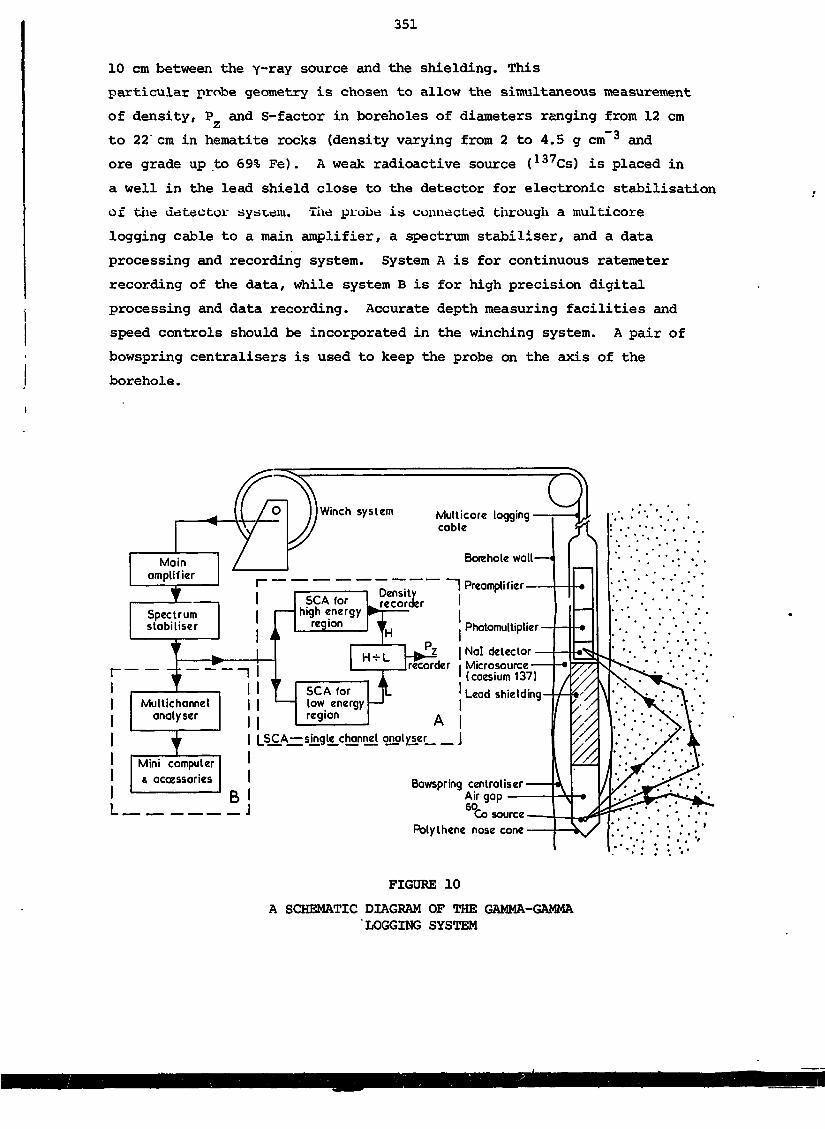
351
10 cm between the y- ay source and the shielding. This
particular probe geometry is chosen to allow the simultaneous measurement
of density, P and S-factor in boreholes of diameters ranging from 12 cmzto 22' cm in hematite rocks (density varying from 2 to 4.5 g cm 3 and
ore grade up to 69% Fe). A weak radioactive source (137Cs) is placed in
a well in the lead shield close to the detector for electronic stabilisation
of the detector system. The probe is connected through a muiticore
logging cable to a main amplifier, a spectrum stabiliser, and a data
processing and recording system. System A is for continuous ratemeter
recording of the data, while system B is for high precision digital
processing and data recording. Accurate depth measuring facilities and
speed controls should be incorporated in the winching system. A pair of
bowspring centralisers is used to keep the probe on the axis of the
borehole.
Winch system
Densityrecorder I
Muiticore loggingcable
Borehole wall
~~\ Preamplifier—
Photomultiplier
Nal detectorMicrosource(caesium 137)Lead shielding
LSCAj^sjngle_channel qnaly_ser
Bowspring centraliserAir gap —
Co sourcePolythene nose cone
FIGURE 10
A SCHEMATIC DIAGRAM OF THE GAMMA-GAMMA'LOGGING SYSTEM

352
Calibration of the probe
There are three basic aspects of calibrating a density-P probe forzapplications in mineral exploration. These are:
(a) calibration of the intensity of the high energy part of the
backscattered yray spectrum for measurement of formation
density,
calibration of the ratio of the intensity of the high energy(b)
(c)
to the low energy region (P ratio) for measurement of theZ
Z (ore grade) of the formation, andeqcalibration of these density and P responses in relation
Z
to borehole diameter.
For logging water or other fluid filled holes, a complete set of new
calibrations is needed.
For calibration in the laboratory, models with accurately known
density, chemical composition and hole diameters are used. The range of
model parameters should be the same as those expected in the field.
QoUJa.
UJ
UJ
I
>
25OO-
_ 2000-
1500
1OOO-
5OO2 3 4 5
DENSITY (g/cm3)
18
15
13
P.0-9
*a
O7
-1,
221813
30 4O SO% IRON
60
FIGURE 11
CALIBRATION CURVES FOR THE DENSITY-P PROBEZ

Figure 11 shows how the probe response for density and. P varieszwith borehole diameter in laboratory models. The density probe response
is extremely sensitive to changes in borehole diameter. Therefore, it
is imperative that an accurate knowledge of the hole diameter is available
to correct the density response. In contrast, the P response is lessZ
sensitive to hole diameter. Here again, for precision work, corrections
for borehole diameter should be utilised. Hole diameter is usually
Example log
The density-P probe was used to log a 14 cm nominal diameterZ
diamond drilled hole in hematite rock. A diamond drill hole was selected
for this log to permit comparison of the probe response with known rock
properties (density and chemical composition) determined by laboratory
measurements on the core. The basis of this comparison was 61 cm (2 ft)
core splits. Diameter of the diamond drill hole varied from 14 cm to 22
cm. The formations through which the borehole passed varied from dense
high grade hematice to low density shale and highly porous class III
hematite mixed with goethite. An example of the density-P .log is presented
in figure 12. The stratigraphy of the formation is also shown.
1O
E
II-O.Illo
15
20I
KDOO 12OO 1400 c/sDENSITY LOG
O-7 O-8 O-9PZLOG
14 16 18 cmCALIPER LOG
Steel casing
High gradehematiteShale band
High gradehematite
Shale band
High gradehematite
Mixture of classII & III hematiteand goethiteShale bandClass II tillhematite andgoethite
STRATIGRAPHY
FIGURE 12
DENSITY-P AND CALIPER LOGS IN HEMATITE ROCKSz

Accuracy
Experience shows that both density and P can be determined with azmoderate degree of accuracy in such a borehole. Thus the average density
of a geological section (complete borehole) can be determined with an accuracy
(lo) of ± 0.03 g cm 3. This is the same order of accuracy quoted for
oil well logging. The accuracy (la) for iron ore grade determination
via P is ± 0.4 % Fe for the average grade of a geological section,z2.3 Density Probe for Oil Well Logging
Gamma-gamma logging for density finds its most important application
in oil well logging for porosity measurement. A different probe con-
figuration is used in oil well logging to overcome the problem of variation
in hole diameter and the problem of drilling mud. In this configuration,
a special bowspring is used to press the probe against the borehole wall
as shown in figure 13. Both the detector and the source are colliroated.
Even though this technique eliminates the problem of mud density and
variation in hole diameter, it gives erroneous results with very rough-
walled holes.
FIGURE 13
SCHEMATIC DIAGRAM OF A SIDEWALL DENSITYPROBE USED FOR OIL WELL LOGGING
Although more accurate probes have been devised, they do not entirely
overcome the problem. It has been necessary to use dual detector systems
to solve this problem.

2.4 Sources of Error in Gamma-Gamma Logs
Borehole effects
We have seen that the gamma-gamma probe response is influenced by
changes in borehole diameter and 'rugosity1 (roughness) of the walls;
in fact these changes give rise to the principal sources of error. With
mechanical calipers, an accurate measure of the diameter of an irregular%..•* . ; , 3; r r: ~.,TI -.-3 : t. * - ~i- ,.». ; —^ ^ . -.; i> . *_ _^ ,.,. -. V-.T- •*•->«•» -.V** ~ e e.llOXC X& CLO.1. Lj.CUJ.t- I U^ilA O.I. .4.O 11.1.AI4WO — J.*ilj.,^0.^.».J-S_ i.. .»t^.lA£>lA .*.>-. «*W-^<_ -. WW*^l*.l«U5d •
Large source-to-detector distance tends to reduce the diameter effect on
the probe response, although this approach also reduces the spatial
resolution of the probe.
The effect of fluid in the borehole is another factor that affects
the probe response. In general, a separate set of calibration curves
has to be used for all measurements in fluid filled holes. Sidewall
probes should be in perfect contact with LKe wall, while centralised
probes should be accurately maintained on the axis of the hole if
introduction of errors is to be avoided.
In the case of density logs in oil wells, mud-cake thickness is an
additional factor which has to be taken into account to correct the
probe response, twin detector probes being used with considerable success.
Z/A effect
We have seen that the Z/A ratio of several elements that constitute
the Earth's crust deviates from the constant value of 0.500. This
deviation introduces an error in bulk density determination. However,
such errors are small and can be neglected in most applications.
Natural radioactivity
Natural radioactivity is present in varying amounts in all geological
formations, and a knowledge of this activity is required to correct the
probe response. Such a correction is negligibly small if the natural
radioactivity is only a small fraction of the scattered y~ ay
intensity. Thus, this error can be reduced by increasing the source
strength.
Statistical fluctuations
If the probe response (number of y-ray signals recorded by the
detector) is low, the statistical error, which is given by the square
root of the number of counts recorded over a given time or a given
length of borehole, can be prohibitively high. This source of error can
be reduced by employing strong sources, more efficient detectors, long
counting periods or slower logging speeds.

356
Error in the calibration curve
Usually, probes are calibrated in models made from natural rocks.
Density and chemical composition of such rocks can and do vary from
point to point. This makes it difficult to obtain an accurate assay of
the density and the chemical composition of the medium within the sphere
of influence of the probe inside the model, and may result in an error
in the calibration curve. Such errors due to geovariance can be minimised
by using a large number of carefully selected and tested models, which
should be free from cracks and voids, and of proven homogeneity.
Effect of temperature on the probe
All radiation detectors and precision electronics are affected by
changes in temperature. In more accurate logging equipment, electronic
stabilisers are used to compensate for changes in temperature of the
probe. Even in cases where stabilisers are used, it is advisable to keep
the temperature of the prote as constant as possible, since stabilisers
have a limited range of performance. Some logging devices use Dewar-
type vessels to keep the detector at constant temperature, although
these reduce the sensitivity of the probe.
Vibration and noise
Precision electronics incorporated in a borehole logging probe are
susceptible to mechanical vibration and noise resulting in modified
probe response. Equipment should be ruggedised and logging speed should
be low enough not to adversely affect the performance of the probe.
?.. 5 Other Applications of Density and P
Techniques in Borehole Logging
The gamma-gamma method for density measurement was introduced in
the early Fifties to aid geophysicists in making allowance for density
variations with depth in gravimetric prospecting. It then found its way
into the technology of oil well logging as a porosity tool of major
importance.
Information on formation density is required to determine porosity,
lithology and the degree of saturation with oil, gas or water. The
density log is useful in identifying rock type where an independent
measure of porosity is available. Adaptation of density logging principles
can be used to measure fluid density in boreholes, and to locate cement
tops behind casing. Gas-fluid interfaces in formations can also be
located.

357
Density logs are helpful for interpreting gravity surveys, identifying
seismic reflecting layers, and estimating ore reserves. If there is a.
strong correlation between density and ore grade, density logs can be
used to measure ore grade directly, as in the case of iron ore. Apart
from grade control, density measurement may provide information of help
in blasting calculations and classification of ore types.
The P method, even though at an initial stage of its development,zfinds its most important application in the detection and evaluation of
heavy minerals associated with light element impurities (e.g. iron ore)
or light element host rocks (e.g. uranium in sandstone). Work by CSIRO
has shown that the mean iron ore grade in a borehole can be determined
with an accuracy of better than ± 0.4 % Fe (la) under field conditions.
Another important application of density and P techniques is inzthe coal mining industry, where density logging can be used to locate
coal strata, and P to measure ash content,z3. BIBLIOGRAPHY
Aylmer, J.A., Mathew, P.J. & Wylie, A.W. [1978] - Bulk Density of
Stratified Iron Ores and its Relationship to Grade and Porosity.
Proc.Australas.Inst.Min.Metall., No.265,
Charbucinski, J., Eisler, P.L., Mathew, P.J. & Wylie, A.W. [1977] -
Use of Backsca-ctered Gamma Radiation for Determining Grade of Iron
Ores in Blast Holes and Development Drill Holes. Proc.Australas.Inst.
Min.Metall., No.262.
Czubek, J.A. [1965] - Physical Possibilities of Gamma-Gamma Logginn.
In Radioisotope Instruments in Industry and Geophysics. Proc.Warsaw
' Symposium, October, IAEA, Vienna, 2, 249-275.
Davisson, C.M. & Evans, R.D. [192] - Gamma-ray Absorption Coefficients.
Rev.Mod.Phys., 24(2)79-107.
Pickell, J.J. & Heacock, J.G. [1960] - Density Logging. Geophys.,
25(4) 891-904.
Tayior, D. & Kansara, M. [1966] - Measuring Density with the Nuclear
Backscatter Method. Nucleonics, 24(6) 54-56.
Taylor, D. & Kansara, M. [1967] - A theory of the Nuclear Densimeter.
Soil Science, 104(1) 25-34.
Tittman, J. & Wahl, J.S. [1965] - The Physical Foundation of Formation
Density Logging. Geophys., 30(2) 284-294.

359
PART C
EXPLORATION AND GRADE CONTROL
NEUTRON LOGGING
by
P.L. Eisler

361
1. INTRODUCTION
Neutron borehole logging probes were pioneered in the USA by the
oil industry during the 1940s and 1950s. The main technical problems
that required solution were the detection .of rock zones containing
hydrogenous fluids, and also how to distinguish between the fluids -
the water, petroleum, and gaseous hydrocarbons [Caldwell 1968]. Al-
though many of the principles governing the design of the probes used by
the mining industry today were established many years ago by the oil
industry [Tittle et al. 1951], the mining industry requires probes of
specialised design because -both the applications and the lithology are
often different to those of the oil industry.
1.1 Typical Configuration of Neutron Probes
The probe configuration, as shown in figure 1, consists of a neutron
source located at one end of the probe, and one or more radiation detec-
tors separated from the source by a space which provides the detectors
Ccntroltscr
Cf source Shockmoun!tng Central iscr
Bismuthshield Anodised aluminium
casing
Armouredcable
FIGURE 1
NEUTRON CAPTURE GAMMA-RAY PROBE.(Not shown: 10B coating of scintillator.)
Silicone rubber shock mounting aroundscintillator may carry 6Li as Li2C03
when epithermal neutron counting is required.
with shielding against direct radiation from the source. The shielding
space is either totally or partly occupied by a dense shielding material,
e.g. Pb, Bi or a tungsten alloy, to attenuate the y ays emitted by the
source. Depending on use of the probe, the shielding space varies in
length from 10 to 200 cm, although the total length of metallic shield-
ing rarely exceeds 20 cm.
The diameter of the probes also varies (from 4 to 10 cm), depending
on the size of drill hole and also on the borehole logging application.
Most diamond-core drill holes (5-7 cm dia.) accommodate only the narrow-
est probes, whereas the bulkier probes designed for either high efficiency
or spectrometry may be used in percussion or rotary drilled borenoles.

362
1.2 Neutron Sources for Borehole Probes
The radiation sources most commonly used for borehole probes are
radioisotopic. They are usually preferred to sealed tube neutron gen-
erators because of their relative cheapness, compactness, and ease of
operation.
(a) The most suitable sources for moisture measurements emit a
large proportion of high energy neutrons, e.g. 21f*Am-Be.
However, slower neutrons (e.g. from 252Cf) are suitable for
logging work based on detecting j-rays emitted via processes
of neutron capture and neutron activation.
(b) The sealed (D-T) neutron tube, used in conjunction with a high
voltage generator built into the probe, has wide application
in the oil industry. The reasons for its wide acceptance are
that it can be operated in a pulsed mode and that the mono-
energetic (14 MeV) neutrons it emits are very penetrating.
Apart from its high cost, an important disadvantage of
using this source is that the target (the area emitting the
neutrons) is located at least 20 cm from the end of the tube.
The sources must therefore be operated at much higher output
rates than radioisotopic sources to produce the same count
rate at the detectors. Radioisotopic sources are physically
very compact and may abut the metal shield if desired.
1.3 The Detectors Used in Logging Probes
For neutron counting, two 3He-Kr filled detectors equip the probe
for neutron counting. One detector is shielded with a cadmium sleeve
and counts only epithermal neutrons. The other unshielded detector
counts all incident neutrons. If the detectors are appropriately
matched, both the thermal and epithermal neutron count rates may be4
obtained. Boron trifluoride proportional detectors are, in practice,
less efficient for epithermal neutron detection because of limitations
to operable gas-filling pressures.
• The most common j-ray detectors for neutron probes are Nal(Tl)
scintillation detectors which have high efficiency and also sufficiently
good energy resolution for most logging applications. However, if
excellent energy resolution is required, high purity germanium detectors
built into cryostats are available for borehole logging. The cooling is
provided by prefreezing the propane-Freon mixture in the cryostat with
liquid nitrogen before logging. Cryostats of this type commonly retain

363
their cooling capability for up to seven hours before refreezing is
necessary [Tanner et al. 1972], i.e. long enough for a day's logging.
1.4 Notations for the Different Neutron Logging Probes
Because different applications of logging with neutron probes
require a variety of detectors, sources and techniques, shorthand
notations are introduced below to denote the different probe configur-
ations. The same notations are also commonly used in die relevant
scientific and engineering literature.
Source Radiation Detected Radiation
Neutrons
epithermal neutrons
thermal neutrons
inelastic gamma-rays
capture gamma-rays
activation gamma-rays
Notation
n-n .epi
n-y
n-act
Each of the above types may have specialised configurations. Two
examples of specialised configurations with applications relevant to
this lecture are the sidewall neutron probe (SNP), and the dual thermal
or compensated neutron logging (CNL) probe.
1.5 The Various Applications of Neutron Probes
There are three main applications for probes equipped with neutron
sources. These are:
(a) the measurement of rock porosity;
(b) the determination of lithology; and
(c) the measurement of the chemical concentrations of sel-
ected constituents.
Rock porosity and overall lithological logging are the most commer-
cially developed techniques because of their relevance to the oil industry.
This industry has been far more vigorous than the mining industry in
developing and using this approach to mineral exploration. The deter-
mination of concentration of chemical constituents is a less tractable
problem than the other two, and is probably of greater interest to the
mining industry than the oil industry.
2. POROSITY MEASUREMENTS
Porosity is defined as the percentage of the volume of a rock that
is occupied by voids.

364
2.1 The Physical Basis for Neutron Porosity Logging
In dry rocks, porosity can be measured as effectively with gamma-
gamma probes as neutron probes. Under this condition, both techniques
depend solely on the fact that changes of porosity cause commensurate
changes of density. In both cases, a basic assumption is that the grain
density of the rock matrix is constant.
Below the water table, however, specially designed neutron porosity
probes have a response predominantly governed by the hydrogen concentration.
Grain density changes then take secondary importance [Hearst 1974] . One
important requirement for reliable measurement, however, is that the rock
pores are totally occupied by hydrogenous fluid [Czubek 1969]. The design
criteria for operating neutron porosity probes below the water table are
discussed below.
The physical processes underlying the operation of neutron porosity
probes are the collisions between fast neutrons and the nuclei of rocks
and mineral ores: Collisions with hydrogen nuclei result in a rapid
slowing down of the neutrons through high and epithermal energies to
thermal energies; the neutrons are then easily captured by nuclei, and
y-rays released immediately after neutron capture.
The epithermal and thermal neutron probes respond only to the
neutron scattering processes. The n-y probe responds to the emission of
y-rays accompanying the capture event. The advantages of using Y~raY
detection are high efficiency and the ability to discriminate against
irrelevant chemical components of the rock matrix. The capture Y~*ays
are emitted with energies that are characteristic of the constituent
elements. Since hydrogen is the element of interest in porosity measure-
ments, some selection for this element is possible by accepting only
those events registered in a narrow energy window established around the
hydrogen capture Y~ray line a?- 2.23 MeV. If desired, even better dis-
crimination is possible by eliminating the spectral continuum from the
signal.
The behaviour of all neutron probes in response to variations of
porosity (i.e. moisture) is primarily governed by the relationship
between the source-detector configuration and the migration length, M,
for a particular radiation being detected within a matrix.
The migration length
The detection event of a particular radiation quantum completes a
history of radiation scattering events that begin with the emission of a
365
neutron from the radiation source. The particular radiations that are
relevant to neutron logging are epithermal neutrons, thermal neutrons
and capture y-xays. Without an intervening detection event, a neutron
or photon quantum existing at any moment in the sequence of scattering
interactions would eventually change into the succeeding form of radi-
ation until, finally, the y-ray emitted with the capture of the thermal-
ised neutron is absorbed in the rock matrix. Capture of neutrons also
occurs at energies above thermal, but this can be disregarded because of
the relatively low probability.
In this context, the migration length for each type of radiation is
related to the mean displacement from the emitting source to those
coordinates in space where the radiations cease to exist in the form
required for detection. For example, if epithermal neutrons have become
thermalised in collision processes, then their existence is no longer of
consequence for a detector of epithermal neutrons.
The transport parameters that individually contribute to the mi-
gration length during each successive stage of scattering are the slow-
ing down length of fast neutrons, L , the diffusion length of thermal
neutrons, L,, and the attenuation coefficient of y-rays, y. The relation-
ships between migration length and the detailed transport parameters are
summarised below:
Detected Radiation Migration Length, M
epithermal neutrons M = Ls
thermal neutrons M = /L 2 + L 2. s d
gamma-rays M = /L 2 + L-2 + 1/yz
Variation of radiation flux with porosity
and source-detector spacing
Because moisture content of the rock affects L and L,, and hences athe migration length, the neutron flux distribution must also be greatly
affected. Figure 2 shows that as the water content of the rock increases,
the radiation flux near the source increases. However, the rate at
which the flux declines with increasing distance from the source r
decreases too. At intermediate distances from the source, a crossover
zone of radiation fluxes exists in which the neutron flux is hardly
affected by changes of the rock's water content. Figure 3 shows this in

366
5 3Wt
f
foo'iirP K • fov »I uw
Thermol (lux
Epithermol llun
FIGURE 2
FT.UX OF CAPTATIONS DETECTED BY NEUTRON PROBES(in units of quanta cm"2 s~1)
AS A FUNCTION OF DISTANCE FROM SOURCE.
1O 2O 3O 4O 5O 6O 7O
DISIANCE FUUM SOUHOt (cm)
another way, illustrating the relationship between the flux integrated
over 4JI radians and the distance from the source expressed in terms of
r. For most rocks, the ratio L,/L varies from between 0 and 1, so thata s
the zone that is relatively insensitive to porosity changes, (i.e. the1 crossover zone'), is situated at about 1.5 r/M from the source, accord-
ing to simplified diffusion theory. This value for the location of the
crossover zone is, of course, only approximate and can only be used as a
guide to the probe design.
Bo
Neutron probe characteristics
• A 1Desired ranges ot operation
. C -.- B -i j lor mineral assoying-A.B.C.
FIGURE 3
SENSITIVITY OF PROBE TO ROCK MOISTUREAS A FUNCTION OF SOURCE DETECTOR SPACING.
S SOURCE TO DETECTOR SPACING(arbitary units)
With this information, the behaviour of probe response can be
predicted semi-quantitatively against porosity changes. Figure 4 shows
this schematically for long, short, and intermediate spaced source-
detector configurations. The short spaced configuration (< 15 cm for
most rocks) is very sensitive to the presence of neutron absorbers as

367
well as to rock moisture. Spacings of between 15 and 30 cm commonly
give probes which are relatively insensitive to moisture changes,
depending on the type of rock. Porosity changes are thus best monitored
with source-detector spacings exceeding 40 cm.
FIGUBE 4
SENSITIVITY OF NECTRON PROBE WITHVARIOUS CONFIGURATIONS OF SOURCE DETECTORSPACING VERSUS POROSITY (OR TOTAL CONTAINED
MOISTURE IN A ROCK).
One other set of facts, that can be understood in terms of the
migration lengths, is that the flux-distance relationship varies most
rapidly in absolute distance terms for epithermal neutrons and most
gradually for capture y-rays. This is because epithermal neutrons have
the shortest migration length, and capture y-rays have the longest
migration length in the same rock.
2.2 Borehole Effects on Neutron Logging
The actual condition of the borehole will have a marked effect on
the response of neutron logging probes unless special allowances are
made in either the design or the operation ~* the probes. The various
conditions causing interference in neutron logging measurements are
listed below:
(a) whether the hole is cased, e.g. by an iron pipe for structural
support, or whether it has been left uncased;
(b) the amount of mud left in the hole after drilling;
(c) the thickness of hard mudcake on the walls of the hole; and
(d) the addition of cement to anchor the casing inside the hole.
Several of the porosity logging methods are designed to overcome
the difficulties due to the mud and casing. However, the neutron logging
methods of determining the chemical concentrations in ores by n-y.;-, n-y,
or n-act methods should be carried out in uncased or so-called 'open'
holes.

The main problem with open holes, and also to some extent with
cased ones, is that borehole diameter variations occur down the hole,
and these will seriously alter the response of probes under most con-
ditions of operation [Caldwell 1968, Allen & Tittle 1964]. Several
aspects of this behaviour are generally evident:
(i) The variation of probe responses to borehole diameter changes
is greater in rocks having low water content than those of
high water content, as shown in figure 5.
lii) The borehole diameter effects on probe response arc greater in
water filled holes than dry ones (figure 6).
(iii) The effect of a short source-detector spacing is to reduce the
commonly observed trend in which count rate diminishes with
increasing borehole diameter, as is evident in figure 7.
There are two effective ways of compensating for borehole diameter
variations. One method entails a calibration of probe response against
known borehole diameter. For this, holes may be drilled into large ore
or rock samples before beginning field operations in a similar lithology.
The other approach is to use dual spaced detectors in a way that compen-
sates for the variations of borehole diameter.
2.3 The Various Neutron Probe Techniques
Although neutron scattering is the greatest single factor affecting
the response of neutron probes, the rate of neutron capture in the rock
effectively provides a scaling factor for the response. As a result,
single n-*1^ and n-y probes are ineffective for quantitative porosity
logging in rocks where there are significant variations of strongly
neutron absorbing constituent elements.
2.3.1 The sidewall neutron epithermal probe
The problems of neutron absorption are greatly reduced by using n-
n . probes, particularly with neutron absorbing elements of low atomic
weight. For instance, a change of 10 jjg g"1 of boron will induce a 2
per cent change in the response of an n-n.. probe, while producing a
negligible change in that of a n-n . probe. Nevertheless, varying
borehole diameter affects the response of this probe, as it affects all
neutron probes, particularly where the drill hole is filled with water.
The sidewall mechanism is designed to minimise the problem. It
features a 'back-up shoe' that presses the probe against the wall of the
borehole allowing it to skid along the face of the wall. Although by
using this probe the diameter variation effect is reduced by a factor of
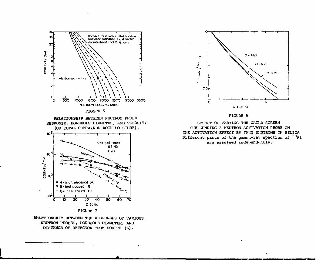
Uncased, fresh water filled boreholelimestone formation 3^"diameterdecentralized tool.C'fcocmg
O 50O 1OOO 15OO 2OOO 25OO 3OOO 35OONEUTRON LOGGING UNITS
FIGURE 5
RELATIONSHIP BETWEEN NEUTRON PROBERESPONSE, BOREHOLE DIAMETER, AND POROSITY
(OR TOTAL CONTAINED ROCK MOISTURE).
10 5
ce
Drained sand95 %H20
• 4-inch,uncased (A)o 5-inch.cosed (B)+ 8-inch cased (C)
i i I I j0 10 20 30 40 50 60 70
Z (cm)
FIGURE 7
RELATIONSHIP BETWEEN THE RESPONSES OF VARIOUSNEUTRON PROBES, BOREHOLE DIAMETER, ANDDISTANCE OF DETECTOR FROM SOURCE (Z).
-a>iZ
A H-O err
FIGURE 6
LFFECT OF VARYING THE WATl'.R SCREENSURROUNDING A NEUTRON ACTIVATION PROBE ON
THE ACTIVATION EFFECT BY FA'JT NEUTRONS IN SILICADif feruut parts of the gamin-i-ray spectrum of
are assessed independently.
23Al

370
between 2 and 4 relative to conventional tools, the effect nevertheless
remains significant and requires systematic correction by using the
signal from the movement of the back-up shoe acting as a caliper.
The SNP has other disadvantageous features. The epithermal neutron
detectors are far less efficient in detecting neutrons than thermal
neutron detectors. The relative efficiency factor lies between 1/10 and
1/100, depending on the gas filling pressure of the epithermal neutron
detector. The detection efficiency can be enhanced to some extent by
surrounding the 3He-Kr counter with a polythene sleeve to moderate the
epithermal neutrons penetrating the outer sleeve of cadmium. The cad-
mium sleeves provide shielding against thermal neutrons.
Other corrections required for the SNP data are the variations of
residual hard mudcake thickness, mud in the hole, and changes in lith-
ology as indicated by density logs.
(i)
(ii)
(iii)
(iv)
(v)
Operational characteristics of the SNP
It is specifically designed for mechanical operation in open
holes.
Source-detector separation is typically 40 cm.
Speed of logging is approximately 10 m min~ 1.
The time constant setting of the recording ratemeter corres-
ponding to this probe velocity is about 2 seconds.
The porosity response, R, is of the form:
A - B*log n
where A and B are constants, and <j> is the observed porosity.
2.3.2 The compensated neutron logging probe
The dual spaced CNL probe is the most effective but also the most
complex of the neutron porosity probes. It effectively eliminates from
its response the borehole effects due to the casing, the diameter and
the mud thickness. The measurement uses the ratio of the individual
responses RI and R2 of two thermal neutron detectors used in the probe.
These detectors are respectively located at lj = 60 cm and 12 = 90 cm
relative to the source. The long spacings are necessary to eliminate
neutron absorption effects from the ratio given by:
where L_, the slowing down length which is primarily determined by
hydrogen in the rock and borehole, is the only neutron transport para-
meter left in the expression. The porosity is obtained from the re-
lationship:

371
log ) = C - D«R2/Ri
where C and D are constants.
One problem remains common to all neutron porosity logs. They do
not provide any way of discriminating between hydrogen as water which is
contained physically within the pores of the rock and that which is
chemically bound as part of the rock's constituent minerals. Of course,
the difficulty is that the neutron porosity measurements are based on
the assumption that variations of the hydrogen concentration reflect
changes in porosity.
As examples, the minerals gypsum and geothite, which are commonly
found, respectively, in oil bearing rocks and iron ore, contain apprec-
iable concentrations of chemically bound water. In the case of gypsum,
the relationship between measured porosity, <J> , and actual porosity, ((»,nis given by:
n + (1 - *) (0.49 G)
where G is the chemical concentration of gypsum expressed as a fraction.
3. LITHOLOGICAL DETERMINATIONS BASED ON MACROSCOPIC CROSS-SECTION
MEASUREMENTS
The purpose of this type of logging is to differentiate between
different geological strata or zones on the basis of changes in the
total macroscopic neutron absorption cross section. Measurements of
this kind are useful where it is necessary to differentiate between oil-
and water-bearing zones, or between disseminated ore zones and host
rock. The basis for differentiating between the various zones is a
monitoring of changes in the macroscopic cross section for a relevant
neutron reaction occurring in the rock matrix as a whole.
One simple, but fairly crude approach to the problem is to assume
constant porosity in the rock matrix, and then to design the source- .
detector configuration of the probe so that varying water content has
minimal effect. A better method uses two sources in the probe which
have different outputs and spacings from the single detector. These
parameters are matched in such a way that the increasing sensitivity of
a short spaced probe to either increasing porosity or rock-moisture, is
balanced by its decreasing sensitivity to increased water content, for
probes with large source-detector spacing.
Typically, the short spacings are between 5 and 10 cm, and the long
spacings are between 30 and 45 cm for sources having their neutron

372
emission rates in a ratio of between 5 and 10, where the more powerful
source is located furthest from the detector. Owing to the approximate
nature of the theory, the probe configuration requires a final empirical
adjustment to realise minimal dependence of the response to slowing-down
length for the particular range of lithologies considered.
In the case of changing grade of ore, the relationship between
probe response and grade is illustrated in figure 8. The only part of
the relationship which closely approximates to linear is in the range of
relatively low grades of ore.
zQ
O5
oa.o
1 o
05
so 100GRADE OF ORE (per cent I
FIGURE 8
THE RELATIONSHIP BETWEEN GRADE OF ORE (ORCHEMICAL CONCENTRATION OF AN ELEMENT) ANDTHE RESPONSE OF A NEUTRON PROBE, i.e. AS
DETERMINED BY THE RATIO OF MACROSCOPIC REACTIONCROSS SECTIONS OF THE ANALYTE (SUBSCRIPT E) AND
AND THE ROCK MATRIX (SUBSCRIPT M).
A method of determining the macroscopic cross section in rock which
is more precise, but which also requires more elaborate and expensive
equipment uses a neutron generator operated in pulsed mode.
Pulsed neutron techniques [Hilchie et al-. 1968] are ideal for
measurement of. the absorptive characteristics of the formation in fluid
filled holes. The parameter of measurement is the lifetime of thermal
neutrons which corresponds to the time interval At3 of figure 9. The
measurement can be used to achieve differentiation between salt water-
and oil-bearing zones in petroleum exploration, or it may show where
highly absorptive imp--,cities, such as boron and rare earths, occur in
rock materials.
The principle of the measurement is that the total number of neu-
trons existing in the matrix at some time t after the occurrence of an

373
impulse burst of N neutrons, is given by:
. Commas from inelastic scattering
FIGURE 9
DIE-AWAY DISTRIBUTIONS IN A ROCK AFTERTHE EMISSION OF A BRIEF BURST ( 5 ys) OF
FAST NEUTRONS
TIME
N exp (-t/T)
where the neutron lifetime T (vnsr is the neutron velocity, and
I is the macroscopic removal cross section of neutrons. In the infinite
homogeneous medium, such determinations would be completely independent
of spatial considerations. But spatial considerations have modifying
effects in the borehole situation, particularly with thermal neutrons,
the fluid in the borehole and the casing material normally produce a
shorter lifetime than the rock; therefore these materials and not the
rock dominate the initial decay of the neutron population sensed by the
detector.
The measurement is made by opening two equally wide time gates at
two different times tj and t2 after the neutron burst. If the recorded
count rates are Rj , and R2 ,
'Rock - £n(R2/Ri)/(t2 -
where £ , is the apparent macroscopic cross section of the formationx\OCJC
and v is the mean neutron velocity, 2200 m s"1.
Several points should be noted:
(i) Erroneous measurements of the formation cross section result
if the first gate is opened too early, so borehole and casing
absorption effects are still significant.
(ii) There is a spatial effect due to a neutron diffusion gradient.
If the detector is too close to the source, more neutrons
diffuse away from the detector than towards it. This has the
effect of reducing the lifetime. But with the detector far

374
from the source the effect is reversed. Typically, results
may be erroneous by as much as 20 per cent. These errors can
be minimised by adding a correction term dependent on the
slowing down length, diffusion coefficient, and source-to-
detector spacing.
(iii) The choice of detector is important, y-ray detectors being
preferred. Neutron detectors give measurements that are
sensitive to the rock only 5 to 8 cm from the hole and are
' therefore greatly influenced by both the borehole fluid and
casing, particularly if the diameter is large. But y-ray
detectors may sample a volume of up to 1 m in diameter. As a
result, neutron detectors are sensitive to probe-eccentricity
in the hole whereas y-ray detectors are not. The latter can
be made sensitive only to the y-rays of t*16 formation by
cladding the detector with boron to absorb thermal neutrons.
The 487 keV energy line emitted in the B(n,ot) reaction must be
biased off.
4. MEASUREMENT OF CONCENTRATIONS OF CHEMICAL CONSTITUENTS OF ROCKS AND
ORES
The principles underlying lithological logging with one or two
isotopic sources of neutrons are of course applicable to the deter-
mination of chemical concentrations of individual constituent elements
in rocks and ores. Lithological logging, as previously considered,
required only detection of radiation without any energy selectivity. A
simple neutron detector or an Nal(Tl) scintillation detector operated
only with a discriminator, to provide a way of blocking electronic
noise, and a sealer are suitable for this purpose.
Apart from a requirement for energy selectivity, borehole logging
to determine chemical concentrations is essentially the same as lith-
ology logging. Energy selectivity is most simply obtained by using a
probe fitted with a spectrometric y-ray detector, and a means of a
nalysing either part or all of the voltage pulse height distribution
output by the detector. The spectral peaks of the pulse height distri-
bution correspond to the y-ray energies characterising the elemental
constituents of the rocks. The continuum on which the peaks sit, rep-
resents the sum of individual spectral Compton continua associated with
peaks having higher energies than the continuum. A typical spectrum
output from a n-y probe is shown in figure 10. The continuum evidently

375
consists of homogeneous information about the elemental composition of
the material, and is basically noise.
I
200
4 6
MeV
FIGURE 10
10
SPECTRUM OF CAPTURE GAMMA RADIATION OFCOAL USING AN ACCELERATOR SOURCE OF NEUTRONS
An energy window placed about a peak in the spectrum thus contains
a mixture of discrete information (the peak proper) and the noise from
the continuum. Any method which is accurately energy-selective aims to
separate the peaks from the continuum. There are many ways of effecting
this but the simplest include approximate fitting of a Gaussian func-
tion, estimation of total peak area by carefully defining the peak
boundaries, and the use of filter function [Op De Beek 1975, Eisler
1976, pp. 158-176].
The rate, R, of detecting gamma-rays in a probe equipped with a
source of neutrons can be expressed conceptually as the sum of two
terms:
R = X + Y
where X is the contribution to the detected radiation by the rock form-
ation and Y is the component generated from within the borehole. As the
source-detector separation increases, Y becomes smaller relative to X,
assuming a constant thickness for the sheath of borehole fluid surr-
ounding the probe. Also, the ratio of Y/X changes commensurately with
changes in thickness of the fluid sheath.
Of course, Y = 0 in dry boreholes, but in water-filled holes of
large diameter, the borehole component, Y, might greatly exceed the
formation component very close to the source. For example, in a 30 cm
diameter hole, X and Y only reach comparable magnitudes 35 cm from the
source.

376
The formation component X is also partly affected by the borehole
fluid, because the y-rays are transmitted through the fluid for detec-
tion. Apart from the low energy photon-radiation, the great majority of
y-rays are hardly affected by the borehole diameter variations that are
normally encountered.
To optimise source-detector configurations for particular cond-
itions, one other concept is helpful. Each of the components X and
Y consists of a term containing the ratio il_/l , where Z_ is the macro-is n Escopic cross section of the assayed chemical element, £.. is the total
Mneutron cross section of the kind of reactions being considered, e.g.
thermal neutron capture, resonance neutron capture and inelastic scatt-
ering, and i represents the relative intensity of the emission y-ray
characterising the chosen element.
However, the macroscopic cross sections E and Z are different inE* M
the borehole and in the rock at each stratigraphic level. For instance,
if the element required for chemical analysis is in the rock but not in
the borehole fluid, 2_/Z,. = 0 within the borehole and consequently Y =E M
0. The case of logging for nickel in an orebody provides a practical
example. -Provided that the nickel concentration within the borehole
fluid (and mud) is negligible, the direct contribution from the borehole
fluid to the counts in the selected y-ray peak due to neutron-nickel
interactions will be negligible. However, if the hydrogen content of
the formation is being logged, as in oil or coal occurrences, the hy-
drogen of the borehole fluid will interfere directly.
As noted earlier, any water in the borehole, and hence any vari-
ation in borehole diameter will affect the neutron flux. Because the
neutron flux is an important factor in both the components X and Y, the
presence of borehole fluid in conjunction with borehole diameter vari-
ations affects the reliability of grade or chemical concentration pre-
dictions based on the y-ray count rate alone.
4.1 Case Studies
In nickel logging trials, using the radiative capture (n,y) re-
action with the characterising emission y-ray line at 9 MeV, the ore-
body was located below the water table. The fit of y-ray counts against
predicted grade was poor. However, when the counts were normalised
according to the measured thermal neutron flux, a good fit to the
regression line was obtained, as shown in figure 11. The capture y-ray
spectra from this borehole logging problem are complex because the iron
concentration varies independently of the nickel. The problem was

377
solved by obtaining calibration response gamma-ray spectra for pure bulk
iron and nickel samples, and then applying a spectral-estimation tech-
nique sometimes referred to as 'the method of mixed channels' [Eisler
1976, De Soete et al. 1972].
FIGURE ID.
RESULT OP FITTING BY REGRESSION THECHEMICAL ASSAYS FOR NICKEL IN SAMPLES FROMCONTIGUOUS BOREHOLE INCREMENTS AND THECORRESPONDING RESPONSES OF THE PROBE
A different facet of a similar logging problem is that of esti-
mating iron ore grades in an open-cut mining situation for grade control
purposes [Eisler et al. 1977]. By contrast with the nickel mineralis-
ation, where the grades of the analyte ranged between 0 and 8 per cent,
the grades of iron in the mineralisation of the Pilbara region of Western
Australia are always high in the mine, ranging from 25 to 69% Fe, with a
.mean of about 62% Fe. one other salient difference between the two
mineralisations was that the logging in the Pilbara was carried out in
dry boreholes above the water table.
These two factors combined to reduce the sensitivity of the y-ray
count rate to changes of iron ore grade, but increased the relative
importance of the moderating properties of the ore-rock matrix. . The
moderating power of the matrix was related in this instance to how much
concentration of host rock was present as contamination in the ore. In
this case, the host rock was a shale, so that the water content was
relatively high (- 12% H20). The ratio of the epithermal to thermal
neutron count rates was therefore an important term for the model used
in the regression analysis of data. In a quasi-operational situation,
where five blast holes were at first chemically analysed for Fe grade,
in small increments of borehole length, the logging trial established
that the mean grade of 61% Fe could be predicted in a new, similar size
blast hole, with a precision of approximately a = 0.4% Fe. The results

378
of the regression analysis, which used about 100 independent data points
are shown in figure 12.
7O-O
£ 6 4 0 -
58-0-
yS 520
CAPTURE DCTA SLAST HOLES 122 en SPLITS
..;<*J
46-O 52 O 58O 64 O TOOCHEMICAL ANALYSIS (%Fe)
FIGURE 12
COMPARISON OF IRON GRADE PREDICTION WITHCHEMICAL ANALYSIS FOR NEUTRON-GAMMA PROBE. •Nominal blast hole diameter 31 cm; logginginterval 1.22 m; 2o for mean grade of single
hole ± 0.7% Fe at 61% Fe level.
Techniques similar to those described above, have been used success-
fully by other researchers and geophysical consultants for nickel,
porphyry copper, and coal deposits [Nargowalla et al. 1977].
Logging rates for the CSIRO trials were 1.5 m rain"1 for the nickel
mineralisation and approximately 0.7 m min"1 for the iron ore. The
reasons for the slow logging rates were a combination of factors. The
sources used were only of moderate strength (107 neutrons s""1), the
detectors were small (50 x 50 mm), and the best counting statistics
possible were reguired for predicting grades of small depth increments
along the hole (<* 0.5 m). It is self evident that scaling up of the
probe parameters would be essential for a field logging operation to
enable faster rates of analysis.
Neutron activation analysis (NAA) is also usefully applied to
borehole logging when the reactions of neutrons with the analytes pro-
duce short-lived radioisotopes (half-life < 10 min). A practical example
is the application of the method to the borehole logging for the alumina
content of shales associated with iron ore deposits in Western Australia
[Eisler et al. 1979]. The method is based on measuring the 1.78 MeV y-
rays emitted by 28A1 (half-life =2.3 min.) formed via the reaction 27Al
(n,Y) 28A1.

379
As with logging techniques that depend directly on measuring the
prompt capture y-rays, (e.g. the logging for Ni and Fe), neutron acti-
vation logging can be either stationary at each of a number of pre-
selected points in a borehole, or by scanning. In the latter mode, the
probe accumulates daui periodically outputs data while moving continuously
in the borehole [Eisler & Huppert 1979]. However, these two logging
modes are more complex for activation logging than for neutron capture
logging.
For fixed point logging, activation at first requires irradiation
of the material surrounding the borehole for a predetermined period
(between one and three half-lives). The probe is then rapidly lowered
by an amount equivalent to the source-detector spacing, enabling y-ray
counting for a specified period. •
In scan logging, the parameters of source-detector spacing and
probe velocity optimised for maximum count rate, are interrelated and
are governed by the half-life of the induced radioisotope. A simplified
expression for the optimum velocity [Eisler 1976, p. 175] is
V . = 0.693 d/T,opt h
where d and T, are respectively the source-detector spacing and the
half-life.
In this context, it is important that sufficient shielding be
provided by both the metallic shielding pieces and the source-detector
separation, to remove all significant interference from competing prompt
reactions [neutron inelastic and (n, y) ].
The experience of researchers at CSIRO was that the best precision
(standard deviation = 0.25 % alumina) of determining the mean alumina
concentration in a drill hole (5% alumina), was obtained for a probe
with a 1.9 m source-detector spacing, incorporating 20 cm of lead shield-
ing, and operating at a logging rate of approximately 0.4 m min"1. The
regression analysis from 23 independent data points is shown in figure
13.
5. DISCUSSION AND SUMMARY
Neutron logging in boreholes encompasses a great variety of tech-
niques that have varying relevance to different sections of the mineral
industry. Two main groups of techniques are well developed both tech-
nically and commercially. They are the methods of porosity and lithology
logging. The applications of these two logging methods are more relevant,
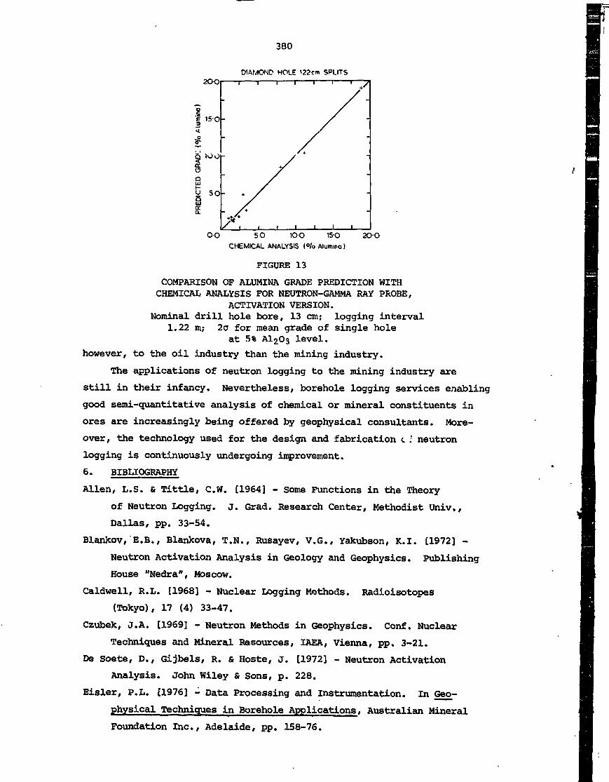
380
DIAMOND HOLE 122cm SPLITS2O-0
15-0
gQ
sE
50-
OO SO 1O-O 15-O
CHEMICAL ANALYSIS (°/o Alumina)
2O-O
FIGURE 13
COMPARISON OP ALUMINA GRADE PREDICTION WITHCHEMICAL ANALYSIS FOR NEUTRON-GAMMA RAY PROBE,
ACTIVATION VERSION.Nominal drill hole bore, 13 cm; logging interval
1.22 m; 2o for mean grade of single holeat 5% A1203 level.
however, to the oil industry than the mining industry.
The applications of neutron logging to the mining industry are
still in their infancy. Nevertheless, borehole logging services enabling
good semi-quantitative analysis of chemical or mineral constituents in
ores are increasingly being offered by geophysical consultants. More-
over, the technology used for the design and fabrication c : neutron
logging is continuously undergoing improvement.
6. BIBLIOGRAPHY
Allen, L.S. & Tittle, C.W. [1964] - Some Functions in the Theory
of Neutron Logging, j. Grad. Research Center, Methodist Univ.,
Dallas, pp. 33-54.
Blankov, E.B., Blankova, T.N., Rusayev, V.G., Yakubson, K.I. [1972] -
Neutron Activation Analysis in Geology and Geophysics. Publishing
House "Nedra", Moscow.
Caldwell, R.L. [1968] - Nuclear Logging Methods. Radioisotopes
(Tokyo), 17 (4) 33-47.
Czubek, J.A. [1969] - Neutron Methods in Geophysics. Conf. Nuclear
Techniques and Mineral Resources, IAEA, Vienna, pp. 3-21.
De Soete, D., Gijbels/ R. & Hoste, J. [1972] - Neutron Activation
Analysis. John Wiley & Sons, p. 228.
Eisler, P.L. [1976] - Data Processing and Instrumentation. In Geo-
physical Techniques in Borehole Applications, Australian Mineral
Foundation Inc., Adelaide, pp. 158-76.

381
Eisler, P.L., and Huppert, P. [1979] - A Nuclear Geophysical Borehole
Logging System. Nucl. Instrum. Methods, 158:578-86.
Eisler, P.L., Huppert, P., Mathew, P.J., Wylie, A.W., and Youl, S.F.
[1977] - Use of Neutron Capture Gamma Radiation for Determining
Grade of Iron Ore in Blast Holes and Exploration Holes. Proc.
Symp. Nuclear Techniques and Mineral Resources, IAEA, Vienna, pp.
215-28.
Eisler, P.L., Mathew, P.J., Youl, S.F. & Wylie, A.W. [1979] - Nuclear
Activation Logging of Aluminium in Iron Ore and Coal. Geoexplo-
ration, 17:43-53.
Hearst, J.R. [1974] - Effects of Bulk Density on Calculated Neutron
Log Response. Nucl. Instrum. Methods, 141:151.
Hilchie, D.W., Mills, W.R., Dennis, C.L., Givens, W.M. [1968] - Some
Aspects of Pulsed Neutron Logging. SPWLA Ninth Annual Logging
Symposium, pp. 1-25.
Nargolwalla, S.G., Kung, A., Legrady, O.J., Strever, J., Csillag, A.
& Seigal, H.O. [1977] - Nuclear Metalog Grade Logging in Mineral
Deposits. Proc. Symp. Nuclear Techniques and Mineral l.-ssources,
IAEA, Vienna, pp. 229-64.
Op De Seek, J. [1975] - Gamma-ray Spectrometry Data and Collection by
Simple Computing Systems. At. Energy Rev., 13 (4) 743-803.
Tanner, A.B., Moxham, R.M. & Senflte, F.E. [1972] - A probe for Neutron
Activation Analysis in a Drill Hole Using 252Cf and a Ge(Li)
Detector Cooled by a Melting Cryogen. Nucl. Instrum. Methods,
100:1-7.
Tittle, C.W., Paul, H. & Goodman, C. [1951] - Neutron Logging of Drill
Holes: The Neutron-Neutron Method. Geophys., 16 (4) 626-658.

383
PART D
ENGINEERING ASPECTS OF RADIOMETRIC LOGGING
by
P. Huppert

385
1. INTRODUCTION
Many engineering problems are encountered in the development of
nuclear borehole logging techniques for obtaining rapid and reliable
stratigraphic and mineralogical information from mine development and
exploration holes. In particular, attention is paid here to those
engineering aspects that require improved precision of measurement and
additional specialised equipment, over and above that required for
electrical, magnetic and other types of borehole logging methods curr-
ently used by industry.
The majority of commercially available nuclear logging systems
are designed for qualitative (stratigraphic) or, at best, semiquanti-
tative usage. In recent years [Eisler & Huppert 1979] nuclear spectro-
metric techniques have been developed that can determine a number of
important elements, such as iron, with relative accuracies of about
± 1 per cent for the mean grade of a drill hole. To achieve these
accuracies, more advanced mechanical and electronic engineering equip-
ment are constantly being developed. For example, the spectrometric
techniques referred to above can provide significantly improved vertical
resolution of stratigraphy, provided that the electronic stability of
the equipment and the precision of depth measurement is better than 1
and 0.1 per cent respectively.
In addition to stability requirements, the electronics must be
capable of handling high count rates of randomly distributed pulses of
fast rise time from the radiation detector. These pulses are processed
by the linear amplifier chain, and then transmitted over a long length
of cable before finally being digitised for computational purposes and
outputting of results.
Two other aspects require special attention. First, spectrometric
systems must be designed so that precise calibration is possible under
field operating conditions. The second relates to the safe handling of
radioactive sources in the field. It must be possible to load the
source into the logging probe without endangering personnel. For this
purpose a specially designed source transporter and carefully rehearsed
operating procedures are required.
2. THE COMPONENTS OF A LOGGING SYSTEM
The principal components of a typical nuclear borehole logging
system are:
(i) The logging probe with its associated logging cable for signal
and power supply connections.

386
(ii) The logging vehicle for transportation of all the equipment to
the mining or exploration site.
(iii) The electronic instrumentation for data collection and pro-
cessing.
(iv) The auxiliary equipment which includes the source transporter,
the tripod, calipers, depth recording equipment, and power
supply for the vehicle. In addition, test equipment and tools
for carrying out repair work are needed.
2.1 The Logging Probe Mechanical Aspects
The mechanical parts of the logging probe, in its simplest form,
consist of four sections. These are, the probe head, the probe barrel,
the nose cone and the logging cable as illustrated in figure 1.
The probe head, which is actually a waterproof seal for the cable
entrance, provides the termination for both the electrical conductors
and the supporting cables. The head should also include provision for the
attachment of a recovery tool in case the probe is 'jammed1 in the bore-
hole owing to its collapse or some other mishap.
As shown in figure 1, the probe barrel houses the sensor, which may
be either a scintillation detector, a proportional counter or any other
suitable nuclear detector. The probe barrel also contains the associated
electronics. Both the detector and the electronics require shock mounting.
Probe head
Cannonconnector
Electronicsbarrel
Shieldhousing
Sourceholder
/Electronics
/Scintillationdetector
Shockmountingi neutronshield
\ /^Isotopic\J neutron
source(b)
, Electronics
' JHe neutroncounters
• Cadmiunshielding
Bismuth shield
Isotopic neutronsource
(d)
FIGURE 1
LOGGING PROBES,(a) Modules of probe assembly; (b) typical
neutron-gamma layout; (c) typicalneutron-neutron layout; (d) caliper
(slip-on type).
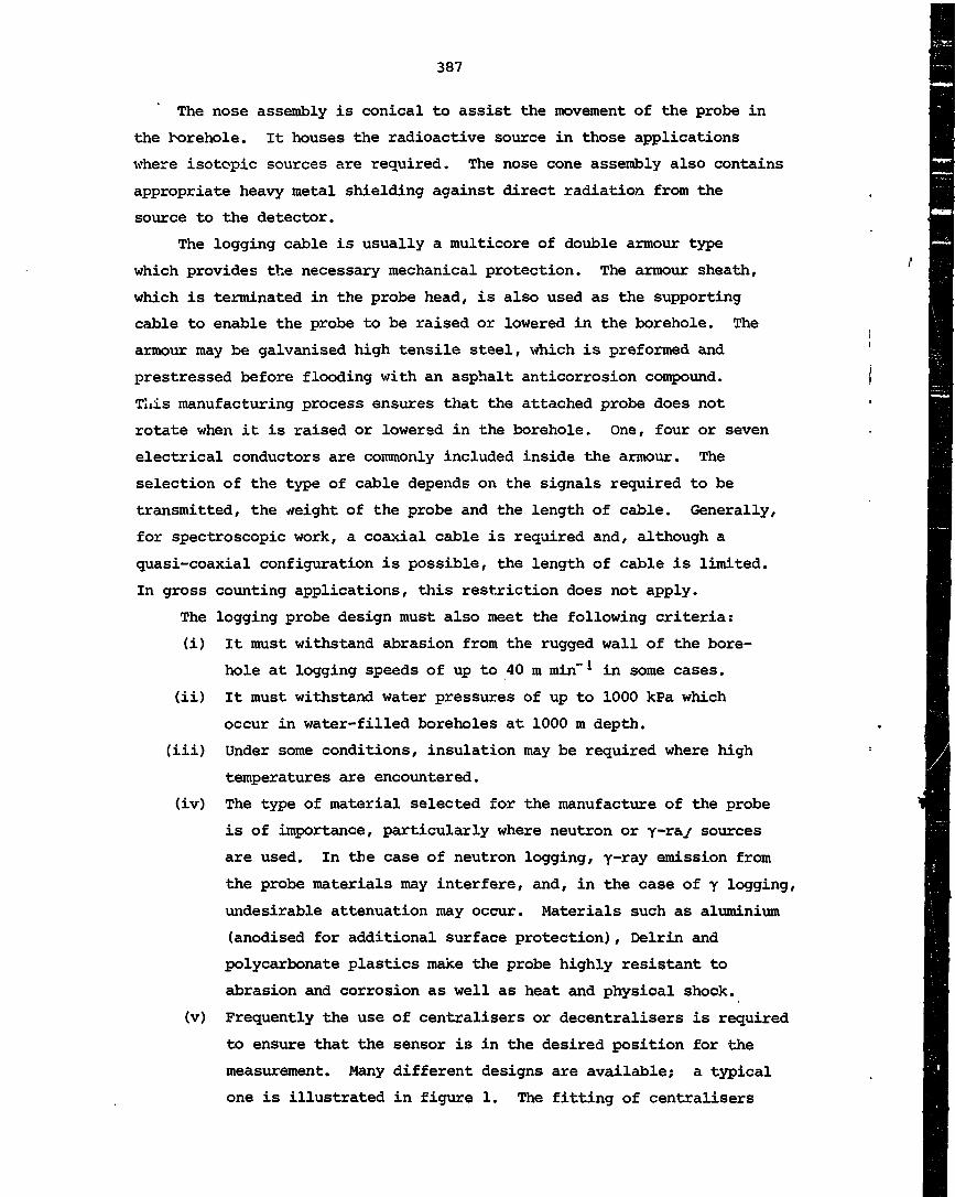
387
The nose assembly is conical to assist the movement of the probe in
the borehole. It houses the radioactive source in those applications
where isotopic sources are required. The nose cone assembly also contains
appropriate heavy metal shielding against direct radiation from the
source to the detector.
The logging cable is usually a multicore of double armour type
which provides the necessary mechanical protection. The armour sheath,
which is terminated in the probe head, is also used as the supporting
cable to enable the probe to be raised or lowered in the borehole. The
armour may be galvanised high tensile steel, which is preformed and
prestressed before flooding with an asphalt anticorrosion compound.
This manufacturing process ensures that the attached probe does not
rotate when it is raised or lowered in the borehole. One, four or seven
electrical conductors are commonly included inside the armour. The
selection of the type of cable depends on the signals required to be
transmitted, the v/eight of the probe and the length of cable. Generally,
for spectroscopic work, a coaxial cable is required and, although a
quasi-coaxial configuration is possible, the length of cable is limited.
In gross counting applications, this restriction does not apply.
The logging probe design must also meet the following criteria:
(i) It must withstand abrasion from the rugged wall of the bore-
hole at logging speeds of up to 40 m min"1 in some cases.
(ii) It must withstand water pressures of up to 1000 kPa which
occur in water-filled boreholes at 1000 m depth,
(iii) Under some conditions, insulation may be required where high
temperatures are encountered.
(iv) The type of material selected for the manufacture of the probe
is of importance, particularly where neutron or y-ray sources
are used. In the case of neutron logging, y-ray emission from
the probe materials may interfere, and, in the case of y logging,
undesirable attenuation may occur. Materials such as aluminium
(anodised for additional surface protection), Delrin and
polycarbonate plastics make the probe highly resistant to
abrasion and corrosion as well as heat and physical shock,
(v) Frequently the use of centralisers or decentralisers is required
to ensure that the sensor is in the desired position for the
measurement. Many different designs are available; a typical
one is illustrated in figure 1. The fitting of centralisers

388
also assists the shock mounting required for the delicate
components inside the probe,
(vi) Finally, the logging probe must be designed so that the
electronics contained in the probe can be easily serviced.
For this reason the logging probe is often of modular design
with removable head and nose cone as illustrated.
The probe electronics
The electronic section of the probe usually consists of a pre-
amplifier designed to suit the detector, a power supply for the pre-
amplifier, a high voltage supply for the detector, and an impedance
matching network to couple the signal from the detector to the logging
cable. The signal is then transmitted to the processing equipment
located in the vehicle.
Many commercially available logging probes also include provision
for spectral energy discrimination and conversion to uniform pulse
height and pulse width. These probes are mainly used for gross counting
rather than spectral counting, which requires multichannel an, ysis.
The detector
The most common nuclear detector used in borehole logging is the
Nal(Tl) scintillation detector. In such a system, the detector forms
the most important link in the chain, which determines the ultimate
resolution and stability. An 'integral1 assembly of crystal and photo-
multiplier is preferred since this type of construction (which eliminates
light losses of the window and provides sounder mechanical coupling
between crystal and photomultiplier tube) is more efficient than the
optical coupling of the demountable crystal and photomultiplier assembly.
The detector assembly must be of a suitable size to fit inside the
small diameter probe, and must also be rugged enough to withstand the
environmental conditions referred to previously. Suitable commercial
assemblies can now be obtained although they are still very expensive.
Good resolution, together with a linear relationship between the
y-ray energy and the resultant pulse height is essential for y spectro-
scopy. Resolution is actually related to the ability of the detector to
separate two adjacent spectral lines. Consideration of this is necessary,
because the pulse height response of the detector to events of one
energy is not just a 'line', but a peak having an approximately Gaussian
distribution about a mean output pulse height. The spread of energy

389
distribution in the peak is a measure of the resolution. This is com-
monly expressed as the full width at the half maximum (FWHM) of the peak,
expressed as a percentage of the mean energy. For scintillation detec-
tors used in borehole logging probes, the best resolution obtainable is
about o.5 per cent t'WHM for the " ' Cs Y~ray at 0.662 MeV. This resolu-
tion drops to approximately 2 per cent at 8 MeV.
The high voltage supply
The high voltage supply for the photomult:plier must be well sta-
bilised as the gain varies approximately according to the relationship.
A£ _ AV~ ' n ~
where G is the gain of the photomultiplier, and n is the number of
dynodes.
With a 12-stage photomultiplier, the change in gain is 8.4 times
the percentage change in supply voltage. Hence to hold the gain stable
to within ± 1 per cent, the power supply must be stabilised to about 0.1-
per cent.
A number of small, commercial photomultiplier power supplies have
recently become available. The units are d.c. to d.c. converters typi-
cally operating from approximately 25 volts d.c. to deliver 1500 - 2000 V
with a maximum power output of the order of 600 mW. ' Regulation to
within 0.015 per cent is achievable.
The power supply requirements can be reduced in those instances
where a 'spectrum stabiliser1 is used to compensate for gain variations,
as described later.
The preamplifier
The preamplifier is mounted as close as possible to the detector to
reduce stray capacitance and maintain good signal-to-noise ratio. It
converts the charge signal from the detector into a voltage or current
output of sufficiently high level for transmission along the logging
cable. Further pulse shaping occurs in the main amplifier, which is
usually located in the logging vehicle.
The output circuit of the preamplifier includes an impedance
matching network of low output impedance, usually with 'sending end'
termination to prevent multiple pulse reflections along the cable
without excessive loading. Typical pulse waveforms that the logging
system has to handle are shown in figure 2.

390
FIGURE 2a
TYPICAL STEP-STAIR WAVEFORM AT INPUT TOCHARGE SENSITIVE PREAMPLIFIER
FIGURE 2b
TYPICAL OUTPUT PULSE SHAPE FROM PREAMPLIFIERO 24 6 8 1O 12 14 16 WITH SINGLE INTEGRATING, SINGLE DIFFERENTIATING
RC TIME CONSTANT OF 2 ys
2.2 The Vehicle
The logging vehicle must be suitable for travelling to remote
locations and be able to carry crew and equipment. Usually a four wheel
drive vehicle is essential. The floor space must be large enough to
accommodate the winch and the electronic instrumentation and to provide
room for storage of other equipment.
A large selection of suitable logging vehicles is available from
commercial geophysical logging manufacturers. Many loggers are also of
the simpler portable or transportable type with limited cable length and
less complex electronics.
• The winch
Many different winch systems are available which vary both in size
and performance. The main requirements are as follows:
(i) The winch speed should be variable, because often a faster
speed is used to lower the probe to the bottom of the borehole
before logging upwards. Speed controls can be either electric
or hydraulic, and the typical range is 0.5 m min"1 to about 40
m min" 1.
(ii) The spooling system is usually of a complex mechanical design
to achieve even laying of the cable on the winch drum,
(iii) The slip rings are an important part of the winching equip-
ment, and should preferably have low noise and 'cross talk1
and low contact resistance.
2.3 The Electronic Instrumentation
The instrumentation fitted to the logging vehicle for data collec-
tion and computation will vary, depending upon whether the equipment is

391
designed for lithology logging (using gross counting techniques) or
quantitative spectre-metric logging for chemical composition.
Figure 3 shows a block diagram of the equipment required for both
types of measurement. The probe output signal is coupled to a spectro-
metric amplifier having both pole/zero cancellation and adjustable time
constants for optimising spectral resolution. The amplified and suitably
shaped signal is then passed to the stabiliser (described later) for any
corrections required due to gain variations resulting from temperature
effects, count rate variations or mains voltage changes.
.SLIP RINGSWINCH
C.TARI1 I^FR
^1 K.
400 CHANNEL
PHA
\
SC
f
A I
\bC
Impedance matchingnetworkCharge sensitivepreamplifierHT generatorPhotomultiplierNal (T f) crystalShieldingRadioactive source
FIGURE 3
SCHEMATIC DIAGRAM OF NUCLEAR GEOPHYSICALBOREHOLE LOGGING SYSTEM
The output from the stabiliser is connected to a number of single
channel analysers and/or to a multichannel analyser. The single channel
analysers (SCA) feed the ratemeters that provide stratigraphic results
in analogue form for outputting on strip chart recorders. The multi-
channel analyser is used for more complex spectrometric analysis, and
will in many instances be interfaced to a computer to handle the com-
putational part of the analysis. The results can be outputted on suit-
able peripherals as illustrated.
As previously mentioned, it is essential that the probe and the
vehicle electronics preserve the proportionality between energy lost in
the crystal by the y-rays and the resultant pulse height of the signal.
Sources of spectrum distortion and degradation of resolution must be
eliminated. The main instrumental causes of distortions that prevail in

392
a spectral y logging system are due to:
(a) Photomultiplier and other gain variations in the electronic
system.
(b) Pulse pile-up.
(c\ Baseline shifts.
Photomultiplier gain variations
These can be caused by changes in interdynode voltages that occur
when the current, drawn by the photomultiplier from its dynode chain,
changes with count rate variations. Other causes are supply voltage,
referred to earlier, and temperature changes. The photomultiplier tube
gain is a function of its temperature, and such temperature changes can
account for several per cent change in gain in the range of 20 to about
25°C which is a typical range over which the probe is operated in shal-
low holes.
One method of compensating for gain variations in the system is to
employ a digital or analogue stabiliser. This .detects any drift in gain
on a statistical basis by means of two 'windows' established on either
side of a reference peak (figure 4). Whenever a count is received in
the lower window, the analogue stabiliser increases the system gain
slightly. However, a count in the upper window leads to a slight de-
crease in system gain. Over a period of time, these counts should be
equal and no net correction will result. Should a drift in gain occur,
one window will begin to receive more counts than the other. The diff-
erence is used to drive a stepping motor or an equivalent electronic
gain element to correct the gain until the counts are once again equal.
I
Peak channel
Lower window Upper window
12O 14OCHANNEL
16O
FIGURE 4
DIGITAL STABILISER "WINDOW"

393
Pulse pile-up
During the recording of pulse spectra, distortions are produced
when two or more pulses occur within the resolving time of the linear
amplifier chain (see figure 5). Because the spacing between successive
pulses is random, 'pile-up1 is unavoidable. This limits the energy
resolution and creates spectral distortions particularly in situations
where high count rates are encountered. The effect can also be important
at moderate count rates, particularly when a low intensity peak must be
extracted from a spectrum containing pile-up due to a much higher intensity
peak.i-| A
B
TIME
FIGURE 5a
PULSE 'B1 APPEARS TO HAVE LOWER AMPLITUDETHAN PULSE 'A', BECAUSE IT FALLS ON UNDERSHOOTOF PULSE 'A1. PULSE 'C1 IS NOT AFFECTED BY
PULSE 'B1.
Resultant
FIGURE 5b
THE EFFECT OF SUPERPOSITION OF THE SMALLERPULSE ON THE DESIRED PULSE AND THE
RESULTANT EFFECT
TIME
The measurement of individual pulses must be independent of previous
ones. The instrumentation needed to correct this effect should ideally
detect each pile-up event and appropriately reject pulses that have
suffered from the resulting distortion. A typical system used to reject
those pulses distorted by the pile-up effect, consists of a logic net-
work which provides an 'inspection period' equal to a single pulse
width. If another pulse occurs during this time, an inhibit signal is
generated to prevent the analyser from accepting the signal for pro-
cessing by the analogue-to-digital converter (ADC; see figure 6). The
time pick-off unit together with the other units shown, illustrates one
of the several possible methods that can be used for such a purpose. A
leading edge timing signal (see figure 7) is obtained from this unit,

394
Linearsignal
Time pick-offsignal
Inspectperiod
Lineardelayed
Inhibitsignal
/\\
i iPeriod during which another timepick-off signal will generate an
[ I inhibit pulse
f\ Delay in linear chain/ \ / \ of PHA prior to/ V \ A D C conversion
1 1FIGURE 6
TIMING FOR PULSE PILE-UP REJECTION
Detector1
Chargesensitive Linearamp amp Delay (part of PHA)
Timepick-off
~1^^^^^i
L, '/Discriminator
f 11J
Inhibitpulse
Inspector Linear gate(part of PHA)
FIGURE 7
MAIN COMPONENTS OF PULSE PILE-UP REJECTION SYSTEM

395
which is connected in series between the detector and charge sensitive
preamplifier. An 'inspect' signal is generated by the timing pulse if
another pulse occurs during the 'inspect period1. An inhibit pulse will
then be generated and applied to the linear gate included in the system
to reject both or all pulses that have occurred during the inspect
period.
Baseline shift
The baseline is the reference line from which pulse heights are
measured by the ADC in pulse height analysers. With AC coupled stages
in the linear chain the baseline will shift up and down, depending on
the shape, polarity (including undershoot) and count rate of pulses.
This shift will cause a distorted pulse height conversion that must be
corrected. Clamping the baseline of the system to a predetermined
voltage level reduces this problem. Some recently manufactured pulse
height analysers now incorporate this feature.
2.4 Auxiliary Equipment
Source transporter
The source transporter serves two purposes. It provides suitable
shielding for the source during storage and transportation and a means
of loading the source into the nose cone of the logging probe.
A suitable mobile neutron transporter is illustrated in figure 8.
The neutron source can be fitted to the logging probe directly from the
paraffin filled transporter by means of a quick release thread on the
source module. This, together with a remote control procedure for
lowering the probe into the borehole, provides the necessary personal
protection. Other types may have side entry and require long tongs for
source transfer.
Caliper
The caliper log is usually the first log undertaken to determine
the general borehole condition and some lithological aspects of the
formation. Presently, the most widely used caliper is the electro-
mechanical type with moving arms or bow springs. These have several
deficiencies, including poor performance in out-of-round holes. For the
irregular holes frequently encountered in the mineral industry, there
are several other principles of caliper operation that offer better
performance.

Bow-spring(four)
i
Walls of drillhole
Hinged aluminiumretaining collar
Clamping screw
Location of NoHTl)scintillation detector
Rodiometric source
Mild steel sourcecapsule
Body of logging probe
Hinged aluminiumretaining collar
FIGURE 9
BOW-SPRING CALIPER

397
A simple and relatively inexpensive device has been developed
(Charbucinski et al. 1976] which can be clipped on to the barrel of a
borehole scintillation probe. The probe can then be used as a borehole
caliper. The device consists of four small radioactive sources of equal
strength located 90° apart close to the walls of the hole, and a detec-
tor which is as close as possible to the centre of the hole (as shown in
figure 9}. If the detector is perfectly centred and if each source is
'a1 cm in from the wall of the hole, the measured intensity (I) for a
circular hole when the radius is R cm will be given by
I =IT (R-a) * (1)
where Q is a constant depending on the nature and strength of the
radioactive sources and on the efficiency of the detector. To obviate
effects due to scattering of primary radiation (1.17 and 1.33 MeV) and
consequent introduction of extraneous instrumental and borehole effects,
all counts are registered in an energy window between 1.1 and 1.4 MeV.
No significant differences in response can then be detected for equi-
diameter holes in different materials. Another useful radiometric
caliper is the combined backscattered gamma radiation probe. This probe
uses spectral intensity data to obtain the 'S' factor, a ratio sensitive
to borehole diameter.
Depth measurement
Depth recording equipment usually consists of a 'sheave wheel' of
known diameter and a revolution counter. The number of revolutions
indicates the length of cable that has passed, and hence the probe
position in the borehole. Variations of this are commercially available
with various degrees of sophistication, e.g. (i) adjustable diameter
sheave wheel to compensate for wear, and (ii) reed switch or servomotor
circuits to generate depth marker pulses. However, the sheave wheel
devices seldom have accuracies better than ± 0.5 per cent, due mainly to
slip, wear, and out-of-true running of the logging cable over the pulley
Cellipsing').
Today, much better accuracy than 0.5 per cent is called for in
matching logging data to the core withdrawn from a diamond drill hole.
For, if properly depth matched, measurements taken during different runs
through a borehole using different investigating probes can often be
combined beneficially to provide various quantitative measurements of
stratigraphy and element abundance.
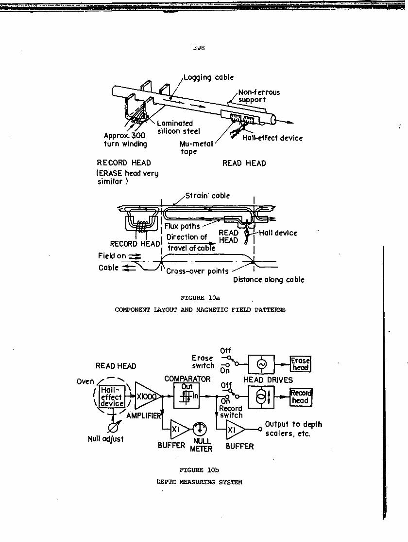
398
Logging cable
Non-ferroussupport
Approx. 300turn winding
RECORD HEAD(ERASE head verysimilar )
Mu-metaltape
Hall-effect device
READ HEAD
Strain cable
Direction ofRECORD HEAD travdofcabte
Field on=g
Cable ^ cross-over pointsDistance along cable
FIGURE 10a
COMPONENT LAYOUT AND MAGNETIC FIELD PATTERNS
READ HEAD
Oven /"—
1\
Hall-effectdevice
\L/
Null adjust
v.^ .Output to depthAl^~~~^ sealers, etc.
BUFFER
FIGURE lOb
DEPTH MEASURING SYSTEM

399
An alternative [Huppert & Millard 1978] to the sheave wheel method
is to use the magnetic properties of the armoured cable sheath, or of
the steel strain cables included in PVC anc" other plastic covered log-
ging cables. The basic principle is that the strain cable or armoured
cable has a magnetic field of reversible polarity implanted on it during
motion, and the resulting cross-over points are used as 'scale marks'.
To create tha scale marks, the cable is passed over a recording head
that will produce the field pattern shown in figure lOa. The circuitry
(figure lOb) is so arranged that when the cross-over point reaches the
read head, located 30 cm (adjustable) from the recording head, it actu-
ates another field reversal in the recording head and increments a depth
counter. The system will therefore self generate accurately spaced
depth markers after manual imposition of the first field reversal and
traverse of this past the detector head.
3. BIBLIOGRAPHY
Eisler, P.L. & Huppert, P. [1979] - A Nuclear Geophysical Borehole
Logging System. Nucl. Instrum. Methods, 158:578-589.
Charbucinski, J., Jarrett, R.G. & Wylie, A.W. [1976] - Radiometric
Calipers for Borehole Logging. Proc. Australas. Inst. Min. Metall.,
No. 258:59-65.
Huppert, P. fi Millard, R.E. [1978] - A Precision Depth Measuring
Apparatus for Borehole Logging. Monitor (Proc. IREE Aust.), 39:47.

401
CHAPTER 8
APPLICATIONS OF RADIOISOTOPE TRACERS
A Series of Lectures
P.L. AireyJ.P. Easey
403
PART A
NUCLEAR HYDROLOGY AND SEDIMENTOLOGY
by
P.L. Airey
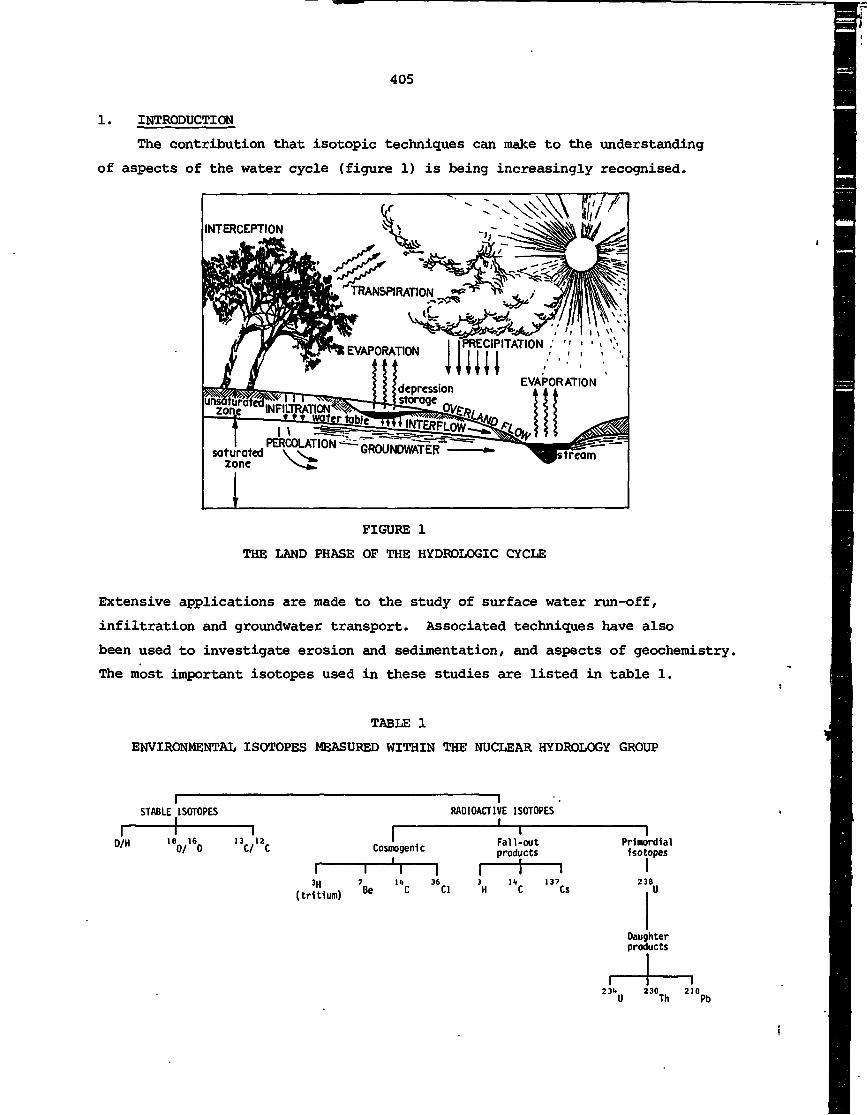
405
1. INTRODUCTION
The contribution that isotopic techniques can make to the understanding
of aspects of the water cycle (figure 1) is being increasingly recognised.
ECIPITATION : ' • ' ' > \v
FIGURE 1
THE LAND PHASE OF THE HYDROLOGIC CYCLE
Extensive applications are made to the study of surface water run-off,
infiltration and groundwater transport. Associated techniques have also
been used to investigate erosion and sedimentation, and aspects of geochemistry.
The most important isotopes used in these studies are listed in table 1.
TABLE 1
ENVIRONMENTAL ISOTOPES MEASURED WITHIN THE NUCLEAR HYDROLOGY GROUP
1 1STABLE ISOTOPES RADIOACTIVE ISOTOPES
I 11 i 1 '/H 80/ 0 ' C/ C Cosroogenic products
i t1 1 1 | 1 1 13U 7 l«i 36 3 111 137
(tritium) Be C Cl H C Cs
PrimordialIsotopes
23
Dau<prot
1
Bu
hteructs
23M 230 210U Th Pb
406
Much of the work of the isotope hydrologist is related to studies
of the dynamics of water and sediment movement. Many applications are
of specific interest to the mining industries. The following are some
typical examples:
(i) Environmental tritium techniques can be used to determine the
origin of water seeping into mines, and therefore assist in the
design of dewatering schemes.
(ii) Low level artificial tracer techniques can be used to
study the distribution of certain components of mine effluents over
a wide geographical area and for long periods. An example is
discussed in section 5. More work of this nature is expected as
the proponents of large-scale mining and industrial ventures seek
to assess in advance the possible environmental impact of the
proposals.
(iii) Systematic surveys of the levels of environmental caesium-
137 can be used to assess the cumulative effect of sediment trans-
port since the advent of nuclear testing in the late 1950s. The
impact of mining and civil engineering on erosion over this time-
scale can therefore be assessed.
(iv) Uranium daughter product disequilibrium surveys can be used
to investigate the dynamics of the accumulation of uranium in
sedimentary deposits. In some cases the data can be used to
determine the potential sources of the mineral.
2. APPLICATION OF ENVIRONMENTAL ISOTOPES TO GROUNDWATER HYDROLOGY
2.1 General Principles
The isotopes of principal interest are tritium (t, = 12.35 y) and
carbon-14 (t, - 5726 y). Both are generated by the action of secondary
cosmic ray neutrons on the components of the atmosphere and as a product
of atmospheric thermonuclear explosions. Tritium is useful for studying
processes over the past few decades; carbon-14 can be used to gain
access to time-scales of the order of thirty thousand years.
Since there are no significant underground sources of tritium or
carbon-14, the levels of isotopes in the groundwater, A, depend on
(a) the specific activity at input, A ;
(b) the extent of radioactive decay;
(c) the effect, if any, of groundwater mixing; and
(d) in the case of carbon-14, the extent, of subsurface
solution of mineral carbonate.
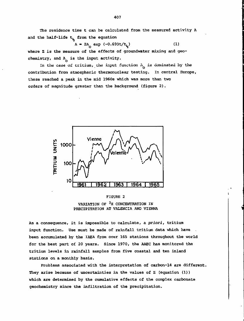
407
The residence time t can be calculated from the measured activity A
and the half -life t, from the equation
A = ZA exp (-0.693t/t, )o *i
(1)
where Z is the measure of the effects of groundwater mixing and geo-
chemistry, and A is the input activity.
In the case of tricium, cue input function A is dominated by the
contribution from atmospheric thermonuclear testing. In central Europe,
these reached a peak in the mid 1960s which was more than two
orders of magnitude greater than the background (figure 2) .
t 1000
Ea:
100
10
Vienna
1961 I 1962 I 1963 I 1964 I 1965
FIGURE 2
VARIATION OF 3H CONCENTRATION INPRECIPITATION AT VALENCIA AND VIENNA
As a consequence, it is impossible to calculate, a priori, tritium
input function. Use must be made of rainfall tritium data which have .
been accumulated by the IAEA from over 165 stations throughout the world
for the best part of 20 years. Since 1970, the AAEC has monitored the
tritium levels in rainfall samples from five coastal and ten inland
stations on a monthly basis.
Problems associated with the interpretation of carbon-14 are different.
They arise because of uncertainties in the values of Z (equation (1))
which are determined by the cumulative effects of the complex carbonate
geochemistry since the infiltration of the precipitation.

408
Three parameters of interest to the practising engineer can be
determined:
(i) The mean residence time of the graundwater. The mean residence
time or age of a groundwater sample in a simple homogeneous aquifer
system can be determined by application of equation (1). The
parameter is important from a practical viewpoint; if the turnover
time of the groundwater is only of the order of a few years, any
over-exploitation can in principle be corrected in a reasonable
time-scale. For instance, in the Burdekin Delta, Queensland a
potentially serious situation developed in the mid 1960s because
of over-irrigation of the expanding sugar and rice plantations.
Water tables began to fall, and as a result there was a potentially
serious problem of sea water ingress, particularly to the productivity
of the coastal farms. In practice, the situation was corrected by
the construction of an extensive series of artificial recharge
channels.
(ii) The delineation of recharge areas, in general the age of
water in a homogeneous system increases with distance from well-
defined recharge areas. The use of isotopic methods to map recharge
areas can be especially useful in remote regions where the number
of observation bores may be insufficient to develop potentiometric
surfaces.
(iii) Groundwater mixing. Most groundwater systems are complex
and replenished by water from different recharge areas. The Burdekin
Delta is typical of many aquifers; localised recharge occurs
through the bed of the river and its tributaries; distributed
recharge over the whole area induced by precipitation is also
important. Careful analysis of the stable isotope ratios D/H and
180/160 can frequently identify different sources. The stable
isotope ratios depend on a number of parameters, but are parti-
cularly sensitive to the temperatures of precipitation. Thus, in
many cases, water from a river with an elevated catchment can be
distinguished from that falling on a flood plain.
2.2 Field applications
Three examples from the AAEC program will be briefly mentioned .
The locations of the field areas are shown in figure 3.

409
Magela Creek (
GW = Groundwater studiesSW = Surfacewater studiesSED = Sediment redistribution
studies
Burdekin Delta(GW)
rokenHilKSED^
9 r%<Xivjc^I
illey (GW)•Ar'midale (SED)
lunter Valley (SED)\ >f I *(SEa *Hl
r VjMprNN-S-W* ^dney(SW)Coonawarra-j I s ,» 7 ' ...Valley (GW) UVlC>~^r
fawaree <GW)
• «• •
las.
FIGURE 3
LOCATIONS AT WHICH THE NUCLEAR HYDROLOGY GROUPHAS UNDERTAKEN RESEARCH PROJECTS
The Burdekin Delta - a tritium study
The results of an extensive survey of the tritium levels in the
Burdekin Delta are summarised in figure 4. As expected, the age of
water increases with distance from the river which is an important
source of recharge. Tritium levels also decrease with increasing depth.
The vertical stratification is an indication of local recharge. The
short residence times indicated by the high tritium levels are consistent
with known hydraulic data. As discussed in section 2.1, it was possible
to correct the effects of over-exploitation by an extensive program of
artificial recharge.
Mereenie Sandstone aquifer, Alice Springs - a carbon-14 study
The study .of the isotope hydrology in arid and semi-arid regions of
the Australian continent, where the potential evaporation rate can
exceed the mean annual rainfall by an order of magnitude, is of particular
interest. A survey of the carbon-14 levels in bores tapping the Mereenie
Sandstone aquifer which supplies Alice Springs with much of its water
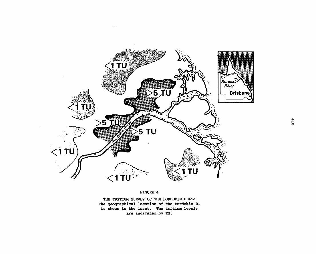
4*HO
FIGURE 4
THE TRITIUM SURVEY OF THE BURDEKIN DELTAThe geographical location of the Burdekin R.is shown in the inset. The tritium levels
are indicated by TO.

411
has been interpreted on the understanding that the recharge rate was far
from uniform over the millennia. Evidence was adduced that recharge
occurred at a somewhat greater than average rate at about 6000 y, at
about 1800 y and a few hundred years before present. Such results
contribute not only to our general understanding of aspects of desert
hydrology, but also to our knowledge of climate in past times. For
instance, evidence is accumulating for the existence of wetter than
average periods about 6000 years ago in other regions of Australia, in
some parts of Africa and in the Middle East.
The Great Artesian Basin(GAB)
To the isotope hydrologist, the principal research interest in the
GAB stems from its enormous size. Up to 500 000 years are required for
water to flow from the infiltration areas west of the Great Dividing
Range to output areas in South Australia. The AAEC has sampled over 100
bores which tap the principal Jurassic aquifer mapped by the Bureau of
Mineral Resources. Such is the age of the water that carbon-14 techniques,
which can date water up to 30 000 y, have been used only to delineate
recharge areas in Queensland and to confirm input areas in South Australia.
The work on the western extremities of the basin is of particular significance
as the density of observation bores is frequently too low to draw firm
conclusions from conventional hydraulic data. The GAB study well
illustrates the potential value of long lived environmental isotopes in
some local basins. Techniques are being developed for measuring the
cosmogenic isotope chlorine-36 which has a half-life of 308 000 years.
This isotope can, in principle, be used not only to measure the age of
• very old groundwater, but also to study the evolution of salinity in the
water.
3. URANIUM DAUGHTER PRODUCT DISEQUILIBRIUM STUDIES
In recent years, uranium isotope ratio techniques have been applied
to hydrological problems. Uranium-234, a second order daughter product
of uranium-238, has a half-life of 248 000 years. Since' 231*u/238U
activity ratios are frequently in excess of unity, the possibility of
using systematic ratios to study the transport of water over the 105
year time-scale has been postulated. Because uranium is found in almost
all host rocks, and it is therefore impossible to define a genuinely
closed system, extensive applications to hydrology have not been made.

412
However, uranium daughter product disequilibria are being increasingly
used to study the evolution of sedimentary deposits. A typical example
is the study of the uranium accumulation at Yeelirrie which is located
in the Murchison region of Western Australia, approximately 700 km
north-east of Perth. The weighted means of the 23l»u/238U and 23°Th/23HU
ratios were 1.38±0.1 and 0.88±0.26, respectively. The larger variability
of the latter ratio is not solely due to experimental factors; it is
taken as evidence for the translocation of uranium subsequent to deposition.
An attempt has been made to interpret the disequilibrium in terms
of 'age1 of the sedimentary deposit. It is accepted that data can only
provide quantitative evidence for or against hypotheses based on geological
and paleoclimatic considerations. It is tentatively concluded that
significant translocation of uranium occurred during the last interglacial
period.
4. ENVIRONMENTAL CAESIUM-137 AND SEDIMENT TRANSPORT
Unlike carbon-14 and chlorine-36 which stabilise chemically as
dissolved species, the fission product caesium-137 adsorbs strongly on
clays and other soil components and can therefore be used as an environ-
mental tracer to study the redistribution of sediment. Small concentrations
of the isotope began accumulating in rainfall during the early 1950s,
from which it was adsorbed on to vegetation and soils in the catchment
areas. Subsequent erosion led to a relocation of caesium-137 to areas
of deposition. Thus in an erosion deposition sequence, location of the
caesium-137 horizon can be used as a mark for, say, the year 1955 which
corresponds to the onset of extensive atmospheric nuclear testing. In
favourable circumstances, it is possible to correlate the caesium-137
soil profile with the differential input of the isotope. The example
shown in figure 5 is the profile from the bed of the Stephens Creek
Reservoir near Broken Hill, NSW. From the results, an average sedi-
mentation rate of 1.6 cm y 1 was calculated. This value is consistent
with that assessed from the historical record.
In other applications, the cumulative effect of sediment relocation
in river catchments can be monitored and the results correlated with
meteorological records and known changes in land use patterns. In
principle the caesium method can be used to quantify the impact of a
mining operation on sediment transport in the general vicinity over the
last twenty years or so.

413
£20
Arbitrary time scale1975 1956
I964
I
24 1
\o •
20N- -to o-
22
ie16
10
8
6
4
2
0
oce
14 JnO SQ,0 Q. 512
HOCz uUJI
z z
0 10 20 30 40
MID-RANGE DEPTH OF CORE SAMPLE (cm)
FIGURE 5
COMPARISON OF (a) 137Cs CONTENT IN SOIL FROM• STEPHENS CREEK RESERVOIR, (b) 137Cs CONTENT IN AUSTRALIAN
RAINFALL, AND (c) RADIOACTIVE FALLOUT DATA FOR SOUTHERN HEMISPHERE
5. SURFACE WATER AND HEAVY METAL TRANSPORT
In many mining operations it is necessary to release significant
quantities of low level waste products to the environment. Nowadays, it
is almost always necessary for proponents of new ventures to prepare
statements on the likely impact of the proposed operations on the environ-
ment. Tracer studies have proved their usefulness in assessing a range
of dispersion processes. Radioactive tracers are particularly well
suited to these applications because:

414
EAST ALLIGATOR R.
ft ,5^ INJECTION POINT/ V PANCONTINENTAL
~ABILUKA (I PC)
10km
INJECTION POINTRANGER( IR)
JABIRU
FIGURE 6
EXPERIMENTAL AREA SHOWING PRINCIPAL RANGERAND PANCONTINENTAL INJECTION POINTS IR AND IPC
AND LOCATION OF MEASURING TRANSECTS R, PCI, PCI AND PC3

415
(i) they can be measured at ultra low levels and can therefore be
used in investigations of transport processes over large geographical
areas and for long periods, and
(ii) they can be used to study the distribution of specific elements
between components of the natural ecosystem.
As an example, a study undertaken for Pancontinental Mining Ltd and
Banger Uranium Mines Ltd on the dispersion of water and zinc through the
Magela system (figure 6} during the summer monsoon flood is cited. In
separate experiments, tritium (3700 GBq or 100 Ci) and 65Zn(30 GBq or
800 m Ci) were injected at IR and IPC at a steady rate over 36 hours.
The specific activity of the isotopes was monitored at the transects R,
PCI, PC2, PC2A and PCS. To allow for dilution effects, the zinc tracer
was monitored as the ratio 65Zn/HTO. The regular decrease of the ratio
with time was attributed to the uptake of the tracer by the vegetation
and the sediment. This was confirmed by the direct counting of a range
of samples. Follow-up surveys were made in the subsequent dry season to
determine the ultimate fate of the radioactive zinc. It should be
emphasised that, because of the enormous dilutions over the substantial
period of the experiment, ultra low-level counting techniques must be
used. The work is therefore fairly labour intensive. Nevertheless, in
view of the type of information which can be obtained, the effort is
well worth while.
6. CONCLUSION
To the practising engineer, the isotope techniques have the inherent
limitation that they reflect the average behaviour of the system over a
time commensurate with the half-life of the isotope. Except in the case
of groundwater tritium, sediment caesium-137 and, of course, artificial
tracer work, the information is heavily biased towards conditions that
existed before extensive human exploitation. The engineer is usually
interested in the past in so far as it reflects the future.
On the other hand, isotopic data can provide information on trans-
port on a regional scale quickly and cheaply. In addition, interpretation
of the results inevitably contributes to an understanding of the geochemistry
of the dynamic system. In the investigation of nature, no technique
stands alone; deep insights are only obtained from a synthesis of all
approaches.

417
PART B
MINERAL PROCESSING
by
J.F. Easey

419
1. INTRODUCTION
In the literature there are numerous examples of the use of radio-
isotopes for industrial tracing experiments. Some of the types of
application are:
Mixing Studies
flow rate measurements
residence time measurements
leak detection
flow pattern studies
silt and sand movement
Transport Studies
Wear and Material Transfer Studies
wear measurement
material transfer
corrosion
Metallurgical Studies
distribution measurements
weighing by isotope dilution
In the next two lectures, techniques are described which have been
and can still be used in the mineral industry. Many of the techniques
also have applicability throughout industry.
In all cases, the important factor is the labelling of the phase
that needs to be investigated. It is necessary to ensure that the label
will remain with the particular phase throughout the process(es) through
which it passes during the experiments. There will normally be a number
of suitable radioisotopes for any such work. The choice of a particular
label will then be dictated by external considerations such as cost,
availability, radiological safety, etc.
In the planning of experiments the following points should be
considered:
Is the radioisotope method the best or the most convenient to
use?
What tracer is required, including:
element or phase tracing;
chemical form of tracer;
availability of tracer;
half life of tracer;
duration of experiment?
What quantity of tracer is required, including:
sensitivity of counting equipment;
counting geometry;
absorption and scattering?
What quantity of tracer can be used, including:
exposure to radiation for personnel and general public;
exposure to contamination for personnel and general public?

420
TABLE 1
SOME RADIOISOTOPES COMMONLY USED IN TRACER STUDIES
Isotope
3H
C
35S
32P
82Br
85Kr
Na
131I
Cs
198Au
51Cr
«*6Sc
1UOLa
ggmTc
Half-life
12.3 y
5760 y
97 d
14.2 d
36 h
10 y
15 h
8 d
2.1 y
2.7 d
28 d
84 d
40 h
6 h
Radiation of Interest(MeV)
$ : 0.18
3 : 0.155
3 : 0.167
3 : 1.71
Y : 0.55 - 1.32
3 : 0.7 Y : 0.54
Y : 1.37, 2.75
Y : 0.36, 0.64
Y : 0.48 - 1.37
Y : 0.41
Y : 0.32
Y : 0.89, 1.12
Y : 1.60
Y : 0.140
Chemical Form
Various organiccompounds
CHsBr, NaBr, etc.
Gas
Na2CO3, etc.
CS2CO3
AuCls adsorbed onpowder
Adsorbed on quartz
80203
La203
Tc pertechnetate

421
Table 1 shows the characteristics of some radioisotopes commonly
used in general industrial tracer studies. A good general text on
radioisotope tracer applications has been written by Erwall et al.
[1964]. Reference shouJd also be made to IAEA publications reporting
the proceedings of IAEA symposia and panel meetings [IAEA 1967,1969,
1976,1977] on industrial uses of radioisotope tracers. Detailed in-
formation can be obtained from these sources on the use of specific
tracers for particular studies.
2. PROCESS MEASUREMENTS
2.1 Flow Rates
There are four important methods for measuring the flow rates of
fluids using radioactive tracers, these are:
{ . The peak-to-peak method.
The total count method.i
The continuous sampling method.
The continuous injection method.
Peak-to-peak method
In this method, the time taken for a tracer to pass between two
detectors is measured. A small amount of a radioactive solution is
injected instantaneously into a pipe in which a liquid is flowing at a
rate Q. Two detectors, mounted a distance L apart on the pipe, record
the passage of the tracer. If the time lapse between the peaks is T
then the linear flow rate, V, can be obtained from the relationship:
v = £ (1)
T
The volumetric flow rate, Q, can be calculated knowing the cross-sectional
area of the pipe, S, from the equation:n - £i§. (2)Q- T
In accurate flow rate measurement, because of longitudinal dispersion of
the tracer, the time interval between the centroids of the peaks is
recorded rather than the actual separation of the peak maxima. Also the
tracer has to be uniformly spread over the cross-section of the pipe
before the first detector is reached.
This method has the advantage that no sampling of the system has to
be undertaken, the efficiency of the detectors is not required and the
amount of tracer injected does not have to be known. As long as the
cross-section of liquid flowing is known, the method can be used both
for pipes and for open channels.

422
Total count method
In this method, a known amount of radioisotope tracer is injected
instantaneously into the fluid and the radioactivity is recorded as the
pulse passes a downstream detector connected to a sealer. The faster
the pulse passes the detector, the fewer the counts that are collected.
The detector has to be calibrated using a static system with conditions
identical to those for the dynamic measurement, i.e. same pipe diameter,
pipe wall thickness, etc. If F is the calibration factor from the
static test, A, the amount of activity added to the fluid flowing at a
rate Q, and N counts are recorded from the detector, then these factors
are related by the equation,
QA.PN
As with the peak-to-peak method, the tracer has to be uniformly
mixed over the stream cross-section.
Continuous sample method
This technique is similar to the total count method. A known
amount of tracer is added to the fluid instantaneously and a sample of
the fluid is withdrawn at a constant rate for the total time that the
pulse of tracer passes a downstream monitoring point. As with the other
methods, the tracer has to be uniformly mixed over the whole stream
cross-section before samples are taken. In an alternative approach, the
passing pulse is sampled at regular intervals and the samples are then
amalgamated. In either case, after the samples have been carefully
mixed, the activity of the composite is measured.
If R is the count rate of the sample, T the time of sampling, F1
the sensitivity calibration factor for the detector and A the amount of
tracer added, then the flow rate Q can be determined since
« " E5 (
This equation has the same form as the total count since the product R.T
can be considered to be the equivalent of N, the number of counts.
Continuous injection method
In this method, the tracer is injected over a period, rather than
instantaneously, to allow equilibrium to be established. Samples are
taken downstream and their activity is compared with that injected. If
the tracer is added at a constant flow rate Qi and activity GI to a
fluid with a flow rate Q and activity CQ, and the sample stream has an
activity C^, then
(3)
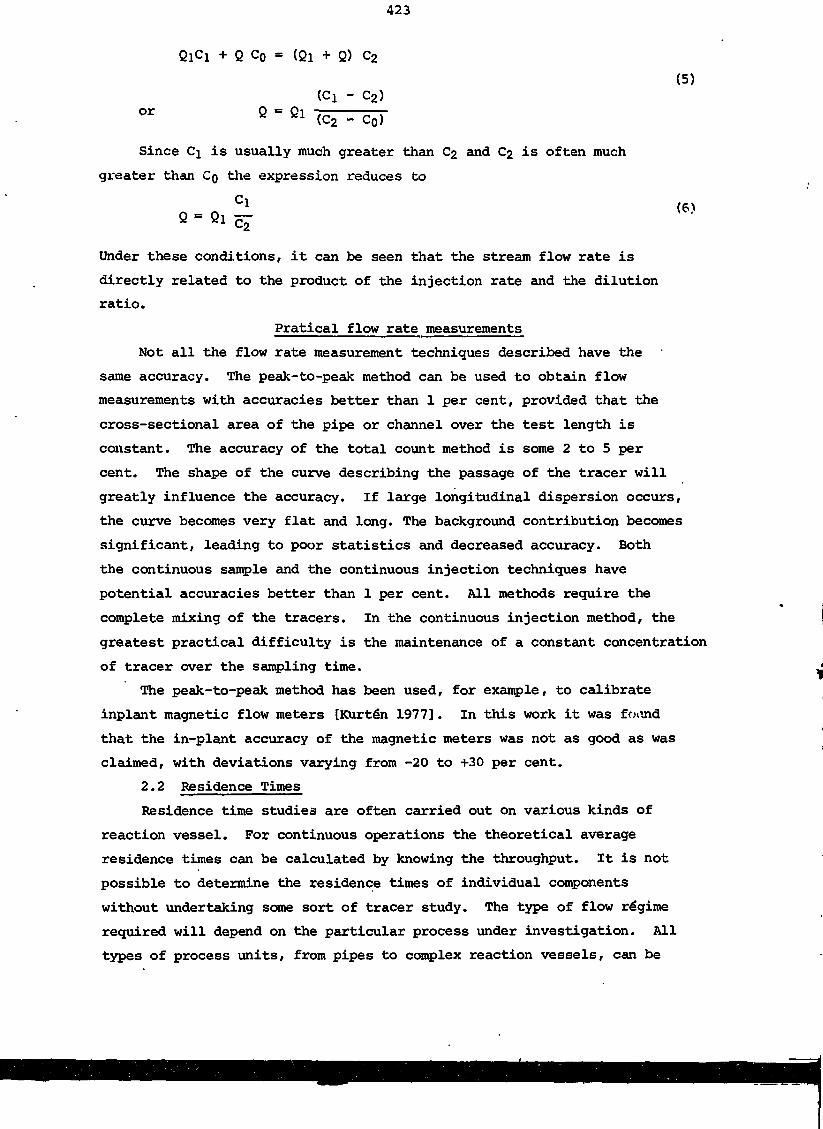
423
+ Q GO = (Qi + Q) C2
(5)
or- C2)
Q = Ql (Q2 - Co)
Since Cj is usually much greater than C2 and C2 is often much
greater than CQ the expression reduces to
(6)Q = Ql C
Under these conditions, it can be seen that the stream flow rate is
directly related to the product of the injection rate and the dilution
ratio.
Pratical flow rate measurements
Not all the flow rate measurement techniques described have the
same accuracy. The peak-to-peak method can be used to obtain flow
measurements with accuracies better than 1 per cent, provided that the
cross-sectional area of the pipe or channel over the test length is
constant. The accuracy of the total count method is some 2 to 5 per
cent. The shape of the curve describing the passage of the tracer will
greatly influence the accuracy. If large longitudinal dispersion occurs,
the curve becomes very flat and long. The background contribution becomes
significant, leading to poor statistics and decreased accuracy. Both
the continuous sample and the continuous injection techniques have
potential accuracies better than 1 per cent. All methods require the
complete mixing of the tracers. In the continuous injection method, the
greatest practical difficulty is the maintenance of a constant concentration
of tracer over the sampling time.
The peak-to-peak method has been used, for example, to calibrate
inplant magnetic flow meters [Kurtdn 1977]. In this work it was foiind
that the in-plant accuracy of the magnetic meters was not as good as was
claimed, with deviations varying from -20 to +30 per cent.
2.2 Residence Times
Residence time studies are often carried out on various kinds of
reaction vessel. For continuous operations the theoretical average
residence times can be calculated by knowing the throughput. It is not
possible to determine the residence times of individual components
without undertaking some sort of tracer study. The type of flow regime
required will depend on the particular process under investigation. All
types of process units, from pipes to complex reaction vessels, can be
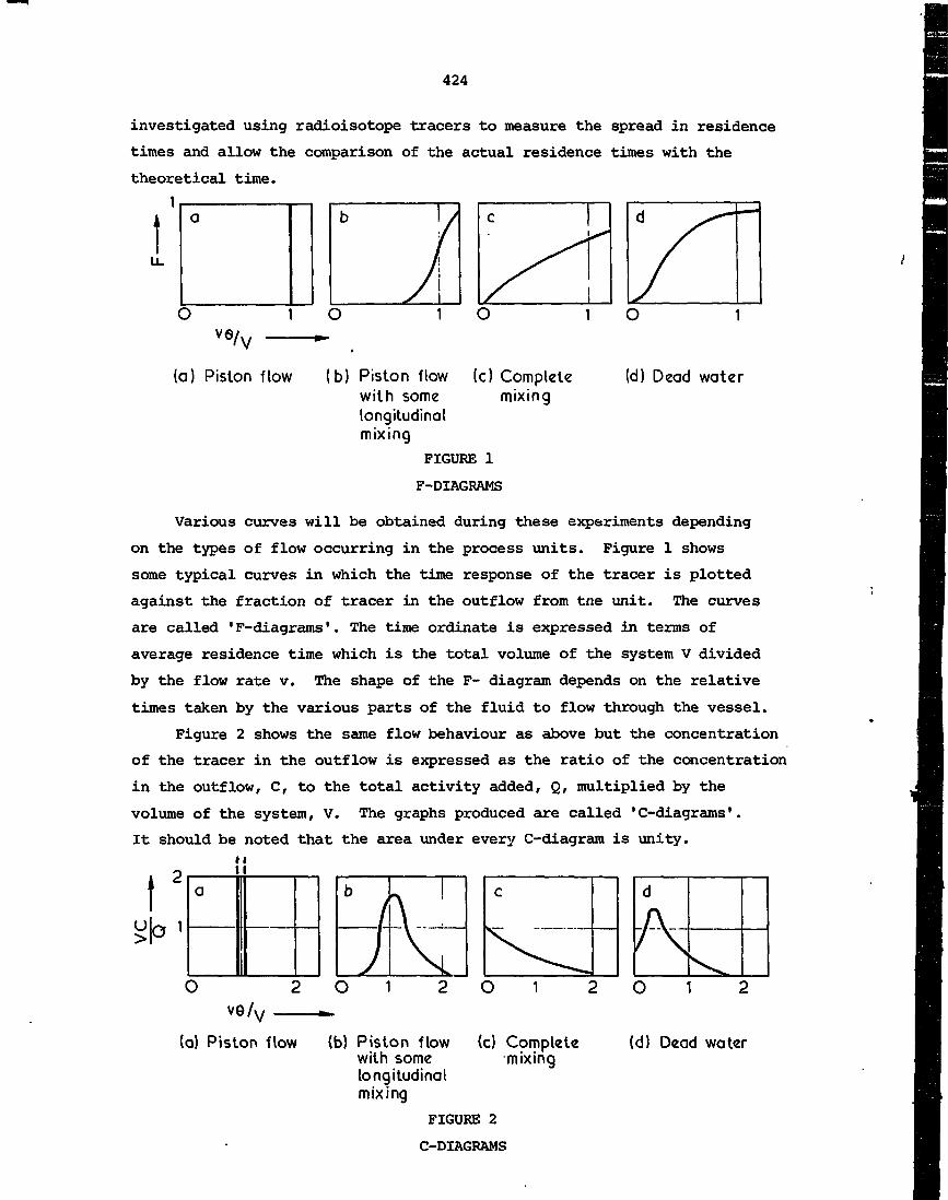
424
investigated using radioisotope tracers to measure the spread in residence
times and allow the comparison of the actual residence times with the
theoretical time.1
u.
O Ove/V
(a) Piston flow (c) Completemixing
(d) Dead water(b) Piston flowwith somelongitudinalmixing
FIGURE 1F-DIAGRAMS
Various curves will be obtained during these experiments depending
on the types of flow occurring in the process units. Figure 1 shows
some typical curves in which the time response of the tracer is plotted
against the fraction of tracer in the outflow from tne unit. The curves
are called 'F-diagrams'. The time ordinate is expressed in terms of
average residence time which is the total volume of the system V divided
by the flow rate v. The shape of the F- diagram depends on the relative
times taken by the various parts of the fluid to flow through the vessel.
Figure 2 shows the same flow behaviour as above but the concentration
of the tracer in the outflow is expressed as the ratio of the concentration
in the outflow, C, to the total activity added, Q, multiplied by the
volume of the system, V. The graphs produced are called 'C-diagrams'.
It should be noted that the area under every C-diagram is unity.ni
UO
a
0ve
a) Pist(
2
'A/
b
;) !0 1 2
r 'V "—
an flow (b) Piston flowwith somelongitudinal
(
(
c
^_^
D 1 2
c) Completemixing
mixing
FIGURE 2
C-DIAGRAMS
d
A/ \
s^O
(d) Dead water

425
There are numerous examples in the literature of the use of radioisotopes
for residence time studies. In some cases it is not possible to produce
exactly either the C- or the F-diagrams because of the nature of the
system under investigation. In a recent investigation by the AAEC, the
residence time of granular pellets in a. devatering unit had to be
measured under various input conditions. The volume of the system for
the solid pellets was not known. Thus it was not possible to do more
than plot the -absolute concentrations of tracer against the absolute
time and compare the residence times for the outflow of certain percentages
of the labelled pellets.
2.3 Mixing and Dilution Studies
Mixing operations are often time-consuming and expensive. If
mixing conditions are net well-known, over-long mixing procedures can be
instituted with a consequent lowering of production capacity and increase
in cost. In a number of systems, overmixing can cause segregation of
components. In cases where the components of a mixture are closely
related or have indefinite chemical compositions, it is often too difficult
or not possible to use standard analytical techniques to determine the
homogeneity of the mix. The use of radioisotope tracers is a cheap and
simple means for optimising a mixing operation. Specific components of
interest are labelled either by neutron activation of suitable elements
in the process material or through an added tracer.
u
TIME
FIGURE 3
VARIATION OF ACTIVITY WITH TIME OF MIXING
The sampling procedure adopted depends on the type of system under
study and, in some cases, on the radioisotope tracer employed. In many
instances it is possible to monitor the dispersion of the tracer using
detectors external to the mixing vessel. With such a system it is

426
possible to obtain at given points a continuous record of the variation
of tracer concentration with time. If, for a variety of reasons, external
monitoring is either undesirable or impracticable, then batch samples
have to be withdrawn from specified positions and then counted elsewhere.
The activity results for samples from one specific point might show a variation
with time, as illustrated in figure 3. The point at which constant
activity is reached can be taken as the achievement of homogeneity at
that point.
There are practical and statistical objections to the use of this
method for assessing such information. In any sampling procedure there
are errors with the analyses of the materials whether they are chemical
analyses or radiation measurements. The preferred method of sampling is
one in which a number of samples are taken at several points for each
time step. The standard deviation s can be calculated knowing each
individual activity A, the mean activity A and the numbers of samples n
from the formula:
£(A - A)2
n - 1
Complete mixing is achieved when a constant variance is reached (see
figure 4).
(7)
HO
} 3-C71O
TIME
FIGURE 4
VARIATION IN MULTIPLE SAMPLES TO DETERMINEOPTIMUM MIXING TIME
toTIME
FIGURE 5
DETERMINATION OF OPTIMUM MIXING TIMEFROM STANDARD DEVIATION MEASUREMENTS
The time of optimum mixing can be found by plotting log s or log(s2)
against time; the point at which the two times intersect is the optimum
time t , as shown in figure 5.

427
The dilution of a radioisotope tracer in a batch process system can
be used to determine mass. A known amount of tracer activity, A ,
which will specifically label a particular phase, is added to a process.
When the tracer has been homogeneously incorporated, the phase is sampled
and analysed. If the sample has a mass x and an activity A then the
total mass of the phase X is given by
(8)
This procedure has been used routinely for such tasks as the determination
of the mass of slag in open hearth furnaces and the mass of mercury in
electrolytic baths.
3. PLANT PERFORMANCE
3.1 Flow Patterns
Residence time studies can provide information on flow behaviour in
continuous process vessels and indicate the presence of dead water, slug
flow, etc. If the actual location of dead water areas or poor mixing
behaviour requires further investigation, flow pattern studies have to
be undertaken. These studies are usually restricted to large vessels,
ponds, etc.
In a recent study by the AAEC, the flow pattern of water passing
through three connected ponds was investigated. A number of transects
were set up across the ponds and the activity of the tracer was recorded
as a function of depth and position as it passed each transect. A
composite picture was then built up of the movement and dispersion of
the tracer in the pond water. Typical results are shown in figures 6
and 7.
3.2 Flow Abnormalities
The flow abnormalities to be considered here are leaks and pipe
blockages. The problems with leaks can be divided into two classes:
one, in which material is lost from the system; and the other, in which
material from one system contaminates another. The most common instance
of the first type of problem is a leaking underground pipe.
The suspect pipe is filled with either a solution or a gas containing
a radioactive tracer and the pipe is pressurised for some time to allow
the radioactive tracer to seep out into the soil around the point of
leakage. The remaining tracer in the pipe is then flushed out and the
detection of the radioactive soil will indicate the position of the pipe

428
FIGURE 6
AREAL DISPERSION OF TRACER IN PONDS
FIGURE 7
DEPTH PROFILE OF TRACER IN POND
'1OOO &Q
!12OO
1400

429
defect. Where shallow soil covers the pipes, the monitoring can be
conducted from above the covered pipe, but where there is more than 1 m
of soil, it is not possible to detect the radiation, hence the radiation
detector has to be pulled through the pipework.
For the second type of problem, common examples are found in heat
exchanger systems. The material that is contaminating, or is suspected
to be contaminating the process has to be labelled with a suitable
radioisotope in a chemical form capable of withstanding the physical
conditions. The process is then run under the required conditions and
the suspected contaminated system is sampled, usually batch-wise, and
counted.
In one study undertaken by the AAEC, heat exchanger oil was thought
to be leaking into a chemical reactor. The volume of the oil system was
6500 L and the contents of the reactor 20 000 L. A " Tc complex having
an activity of 37 GBq was injected into the heating oil which was held
between 200 and 270°C. The chemical reactor was sampled over its eight
hour cycling period. No activity was detected in the reaction product.
The sensitivity of the system was such that a total leak of 85 mL could
be readily detected.
3.3 Wear Measurements
Wear of industrial machines is a perennial problem and one that is
of significant economic importance. Radioisotopes can be determined at
very low levels, so there is a high inherent sensitivity in their use
as tracers for wear studies.
Wear studies have been carried out to determine the abrasiveness of
coal and other minerals on grinding balls. The balls were neutron-
irradiated to produce 59Fe. After grinding the materials with the
irradiated balls, the radioactive iron wear debris was separated from
the ground material by acid leaching and the leachate was counted to
determine the wear rate. These methods have the potential to measure
wear rates involving only 10 g of metal. The AAEC has undertaken
studies of this type to measure the abrasiveness of various grades of
coal.
Wear studies have been carried out by the AAEC on the wear of
components in fuel pump systems used in jet engines. As well as
determining wear regimes, the work was used to assess the suitability of
anti-wear additives and determine their optimum concentration. Typical
results are shown in figure 8.

430
50O
jn"!>•-f
|
01
4OO
3OO
o 200ui
Ou)
I100
No. 17Wear rate 2.76
No. 13 AWear rate 1.17
No. 16Wear rate 1.33
2O 4O 6O 8O 1OOTIME (min)
12O 14O 16O
FIGURE 8
EFFECT OF LUBRICITY ADDITIVES ON WEAR RATE
4. REFERENCES
18O
Erwall, L.G., Porsberg, H.G. & Ljunggren, K. [1964] - Industrial Isotope
Techniques, Munksgaard, Copenhagen.
IAEA [1967] - Radioisotope Tracers in Industry and Geophysics (Proc.
Symp.Prague, 1966), IAEA, Vienna.
IAEA [1969] - Nuclear Techniques and Mineral Resources (Proc. Symp.
Buenos Aires, 1968), IAEA, Vienna.
IAEA [1976] - Nuclear Techniques in Geochemistry and Geophysics
(Proc.Panel Vienna, 1974), IAEA, Vienna.
IAEA [1977] - Nuclear Techniques and Mineral Resources (Proc. Symp.
Vienna, 1977), IAEA, Vienna.
Kurte"n R. [1977] - Int.J.Appl.Radiat.Isot., 28:823.

431
PART C
EFFLUENT MANAGEMENT
by
J.F. Easey

433
1. DESIGN DATA
1.1 Dilution and Dispersion in Natural Systems
Radioisotopes have been used to study the dilution of natural water
systems to obtain data necessary to allow the correct design of effluent
release structures and the optimum design of effluent release procedures.
Depending on the time-scale over which experiments are to be conducted,
a number of radioisotopes such as Tc, Na, Br and T have been used.
COUNTRATE >1MABOVE
BACKGROUND e00 ISO°400 (00
100 400
. FIGURE 1
MOVEMENT AND DISPERSION STUDIES(a) TYPICAL BOAT MONITORING STRATEGY
(b) CONSTRUCTED ISOACTIVITY AREAL DISPERSION
The AAEC has employed two techniques to monitor the movement and
dispersion of the tracer. In one, a number of fixed transects are set
up across the waterway and the variations in tracer activity are
measured at known positions across the transect and at a variety of
depths as the tracer plume passes. This technique is similar to that
used in the flow pattern studies (see Chapter 8, Part B, section 3.1).
In the second method, the peak of the tracer pulse is traversed by boat
as it moves in the waterway. The boat position is continually fixed by
surveyors or instruments (radar, range finders, etc). Depth variations
are measured at the various locations. By noting the times for position
fixing and recording the activities, a picture can be built up of the
expanding tracer plume. A typical boat traversing strategy is shown in
Figure la; in Figure Ib is an example of an isoactivity contour diagram
that is built up from the combination of position and activity readings.
By injecting known amounts of tracer it is possible to relate the recorded

434
activities to dilutions.
The AAEC has made use of tritiated water (HTO) in a number of
studies of natural systems. Since tritium (T) is an isotope of hydrogen,
the tritiated water is a conservative tracer for water whereas the use
of solutes can be criticised on the basis that they do not fully mirror
the behaviour of the water. Because T only emits a weak 18.5 keV
p-particle and no -,-ray, it is not possible to monitor the passage of
the tracer directly, which can be a limitation under some circumstances.
For long-term studies, HTO has shown itself to be a very useful tracer
material. Typical results from such a study are shown in figure 2.
FIGURE 2
SCHEMATIC REPRESENTATION OF A TRITIUM PULSETRAVERSING A TRANSECT
1.2 Movement and Uptake of Solutes in Ecosystems
In Australia there is considerable pressure on large-scale in-
dustrial and mining ventures to assess the environmental impact of their
proposed operations. Of particular importance in these assessments is
the prediction of the environmental effects of low-level effluent re-
leases. The AAEC has used low-level counting (LLC) techniques to support
this type of study. These techniques have been developed over a number
of years in support of various research programs. Highly reliable
nucleonic counting systems are available with sufficient stability to
allow counting over many days and this, coupled to a Y~raY energy analysis
system, allows very low levels of radiation to be detected. A typical
layout for -y-ray LLC is shown in figure 3.
The basic units are the detector, the multichannel analyser and
associated electronics. Lithium-drifted germanium solid state, sodium
iodide or caesium iodide detectors can be used. For routine LLC at
Lucas Heights, a 150 x 100 mm Nal(Tl) crystal in a shielded facility has

435
Detector
Amplifier
Multichannel
Analyser
Printeror
Plotter
FIGURE 3
TYPICAL LAYOUT FOR Y-RAY SPECTROMETRY
Rolling Lid
< </\
/\
/\
/\
/\
/\/\
<
'X <
(
<
< (*
i
K^»
^
w
• . ^^^" •+,
V
V— . .V
V
^.< <
FIGURE 4
SHIELDED Y-RAY COUNTING UNIT
Pb Cell Wall
Cu Lining
Cd Lining
Nal Detector

436
been used. The shielding is a 100 mm thick lead castle lined with
cadmium and copper sheet to absorb excited X-radiation. A diagram of
the system is shown in figure 4.
In studies carried out by the AAEC, the behaviour of zinc and
manganese has been studied in a flood plain environment. The zinc, as
Zn, was injected over 30 h into the flood plain water. The long in-
jection time was necessary to even out any tidal effects. Water samples
were taken at fixed traversing points across the flood plain. Suspended
sediment in the water samples was filtered out and the amounts of Zn
in the sediment and in the aqueous phase were measured. Knowing the
amount of Zn injected, it was possible to determine the amounts of
Zn in solution, adsorbed on suspended sediment, and held up by adsorp-
tion on the bed materials and vegetation between the injection point and
the traversing points. Samples of bed materials and vegetation were
removed to confirm Zn adsorption. With daily monitoring, it was also
possible to measure the subsequent desorption of Zn from areas upstream
of the traversing points. All these measurements allowed predictions to
be made on the impact of low levels of zinc in waste water discharges.
2. EFFLUENT BEHAVIOUR
2.1 Dispersion and Movement of Discharged Effluent
In existing industrial operations it is necessary to verify that
the discharged effluent is behaving in a predicted or predetermined
manner. Because of interference from other sources it may not be poss-
ible to differentiate between the discharge and other material in the
water system. The sampling and monitoring requirements for this type of
work are in essence those described in section 1.1. The tracer material
has to be matched to the requirements of the system depending , for
example, upon whether solutes or solid matter have to be traced.
Work has been carried out by the AAEC on the dispersion and move-
ment of a discharge containing a small fraction of grease. It was found198that the grease could be readily labelled using Au and the tracer was
very adherent to the grease surface. It was found that when the effluent
was discharged into the ocean it formed a surface-trapped layer which
was not readily depth-dispersed by most combinations of wind and wave
action.
Combinations of weather and tide were studied to determine what
conditions cause the deposition of grease on to neighbouring beaches.

437
2.2 Leakage from Waste Storage Systems
Waste waters lost from storage dams, holding ponds, etc. can have
significant effects if they enter ground water or surface water systems
used by others. These leaks may be detected using radioisotope tracers.
Information on the transport rate and the distribution of the tracer can
be obtained by sampling boreholes around the seepage area. It should
also be possible to identify the zones through which the leak occurs. A
variety of radioisotopes have been used for this work but there are
possible problems in relating the behaviour of tracer solutes to the
behaviour of water because sorption processes can take place. The
preferred tracer is tritiated water because it will be a conservative
tracer for water (see section 1.1). Further investigations on the
behaviour of specific solutes in the waste water can be assessed using
the appropriate radioisotopes.
It is sometimes possible to undertake seepage studies using the
environmental levels of tritium present in natural waters. The natural
level of tritium in rainwater varies depending on season and locality
but in Australia generally lies between 5 and 15 tritium units (1 TU =
1 x 10"18 T atoms/H atoms). The half-life of tritium is 12.26 y, so
seepage through rock over long time scales (about 30 years) can be
studied. Comparison of tritium levels in the storage systems with those
levels at the sampling points can yield information on seepage problems.
1

439
CHAPTER 9
RADIATION SAFETY
Two Lectures
D.A. Woods

441
PART A
IONISING RADIATIONS
by
D. A. Woods

443
1. IONISATION AND IONISING RADIATIONS
When nuclear radiation falls on an atom, there is a statistical
probability that an electron will be removed from the atom, leaving a
positive ion. The electron remains free for a very short time and
usually attaches itself to another atom, forming a negative ion. This
is called ionisatiou and an ion pair has been created. Radiations which
produce ionisation are known as ionising radiations.
When ionising radiation falls on biological tissue, ionisation
which can lead to biological injury takes place.
2. DOSE UNITS
In radiation dosimetry there are three different dose units, namely,
exposure, absorbed dose, and dose equivalent.
Exposure is a measure of the amount of ionisation in air. The unit
of exposure is the roentgen (R), which was originally defined as the
amount of X or y radiation required to produce one electrostatic unit of
charge of either sign in air per cubic centimetre of air at standard
temperature and pressure.
In more up-to-date units:
1 R = 2.58 x 10"1* C kg"1
The new SI unit of exposure is the coulomb per kilogram, a much larger
unit than the roentgen.
Absorbed dose is a measure of the energy absorbed from ionising
radiations per unit mass of the absorbing material. The unit of absorbed
dose is the rod, which was originally defined as the amount of ionising
radiation required to produce 100 ergs per gram in the absorbing medium:
1 rad - 0.01 J kg'1
The new SI unit of absorbed dose is the gray (Gy), which is the
amount of ionising radiation required to produce one joule per kilogram
in the absorbing medium:
1 Gy - 1 J kg"1 = 100 rad
In biological systems the same degree of damage is not necessarily
produced by the same absorbed dose of different types of ionising radiation.
To take account of this we use the dose equivalent unit:
dose equivalent = absorbed dose x quality factor (QF)
This was originally called the RBE (relative biological effectiveness)
dose. The unit of dose equivalent is the rem (roentgen equivalent man),
and the new SI unit is the sievert '3v):
1 rem = 1 rad x QF
1 Sv = 1 Gy x QF = 100 rem

444
Table 1 indicates the quality factors for various types of ionising
radiation and table 2 summarises radiation dose units.
TABLE 1
QUALITY FACTORS
Type of Radiation Quality Factor
beta
alpha
X-rays
y-rays
thermal neutrons
fast neutrons
1
20
1
1
3
10
TABLE 2
RADIATION DOSE UNITS
Type
Exposure
Absorbeddose
Dose
Old Unit
roentgen
rad
rem
Symbol
R
r
rem
New Unit
coulomb perkilogram
gray
sievert
Symbol Conversion
C kg'1 1 R = 2.58 x Kf1*
C kg'1
Gy 1 Gy = 100 r
Sv 1 Sv = 100 rem
3. NATURAL BACKGROUND RADIATION
Everyone is exposed to natural sources of ionising radiation. This
natural background radiation varies from place to place, depending on
the radioactive content of the rocks and soils in the locality, the
altitude, the latitude, the building materials, etc. Small amounts of
natural radioactive material, mainly potassium-40, are incorporated
within our bodies. The food we eat, the air we breathe, the water we
drink all contain trace quantities of naturally occurring radioactive
elements.

445
Table 3 indicates typical annual whole body doses caused by natural
background radiation.
TABLE 3
TYPICAL ANNUAL WHOLE BODY DOSESFROM NATURAL BACKGROUND RADIATION
Terrestrial radiation
Cosmic radiation
Internal radiation
Total
Annual
(mSv)
0.5
0.3
0.2
1.0
Dose
(mrem)
50
30
20
100
One millisievert per year (or 100 mrem per year) is an averaged
world figure and is rounded so that it is easy to remember. Obviously
the natural background varies from place to place. In two places,
Espirito Santo State in Brazil and Kerala in Southern India, the natural
background dose rate is as high as 20 mSv per year (2000 mrem per year);
it is caused by beach sands (monazite) containing natural thorium.
4. ICRP DOSE LIMITS
The International Commission on Radiological Protection (ICRP)
publishes safety recommendations periodically. Various countries may
then adopt these recommendations into their own national legislation,
usually in the form of a radioactive substances act. The most recent
publication giving dose limits f>r radiation workers is ICRP 26 (adopted
in 1977); before that, the recommendations of ICRP 9 (adopted in 1959)
were used. Table 4 summarises the ICRP 9 dose limits and table 5
summarises the ICRP 26 dose limits.

446
TABLE 4
ICRP 9 DOSE LIMITS (pre 1977)
Organ orTissue
Gonads and
bone marrow
Skin and
bone
Thyroid
Hands , forearms ,
ankles and feet
Other single
organs
Maximum PermissibleDose for Radiation
Worker
5 rem/year
3 rem/quarter
30 rem/year
15 rem/quarter
30 rem/year
15 rem/quarter
75 rem/year
40 rem/quarter
15 rem/year
8 rem/quarter
Dose Limit forIndividual Membersof the Public
0.5 rem/year
3 rem/year
3 rem/year
except for children
< 16 years for whom
1.5 rem/year
7.5 rem/year
1.5 rem/year
TABLE 5
ICRP 26 DOSE LIMITS (post 1977)
Organ orTissue
Whole body
Gonads
Breast
Red bone marrow
Lung
Thyroid
Eyes
Other single organs
Skin
Dose Equivalent Limitfor Radiation Workers
(mSv/year)
50
200
330
417
417
500
300
500
500
S = StochasticNS = Non-stochastic
S
S
S
S
S
NS
NS
NS
NS

447
In ICRP 26, stochastic and non-stochastic effects are defined as
follows:
Stochastic effects : Probability of effect occurring, rather than
its severity, is regarded as a function of dose, without threshold.
Non-stocJiastic effects : Severity of effect varies with the dose,
and for which a threshold may occur.
5. DOSE RATE
The annual whole body dose equivalent limit for radiation workers
is 5 rem or 50 mSv (unchanged from ICRP 9 to ICRP 26). Pro-rating this
over 50 weeks gives 100 mrem/week or 1 mSv/week. Pro-rating this over a
40 h week gives 2.5 mrem h 1 or 25 ySv h 1; i.e. a person working for 40 h
per week for 50 weeks per year with a dose rate of 2.5 mrem h"1 or 25
ySv h 1 will receive the annual limit of 5 rem or 50 mSv.
Note: To convert mrem h 1 to ySv h 1 simply multiply by 10.
6. POTENTIAL HAZARDS OF IONISING RADIATIONS
Human senses cannot detect ionising radiations, therefore, we must
rely on instruments capable of detecting them to give us warning of
potential exposures.
Radiation injury to people can be classed in two main ways:
(a) Somatic effects^ where the effects occur in the exposed
individual, and
(b) Genetic effects^ where the effects occur in the exposed
individual's descendants.
Somatic effects can be subdivided into:
(a) Acute effects, which occur when a large exposure is received
over a very short time. Here we must protect the worker from
large, accidental exposures.
(b) Late effects^ which can occur when low exposures are received
continuously over a long period of time. Here we must keep the
worker's radiation exposure within the acceptable dose limits set
by ICRP.
When persons are exposed to ionising radiations which are outside
the body, this is known as an external radiation exposure. When persons
take radioactive material into their bodies (by inhalation, ingestion
or absorption through the skin) this is known as an internal radiation exposure.
Radioactive sources may be sealed (e.g. y radiography source) or
unsealed (e.g. radioactive tracer). Unsealed radioactive sources may
give rise to surface or airborne contamination. The working environment

448
must be monitored for external radiation, surface contamination and/or
airborne contamination when these hazards are likely. The worker must
be monitored for personal radiation exposures and personal contamination.
7. TYPES OF IONISING RADIATIONS
Alpha-particles are helium nuclei. They have a very short range in
air and are easily shielded. They penetrate less than one tenth of a
millimetre in human tissue, which is less than the thickness of the dead
layer of skin, and therefore are not considered an external hazard.
However, if alpha-emitting material is taken into the body, alphas can
be considered a very significant internal hazard.
Beta-particles are electrons and have a greater penetrating ability
than alphas. Their range varies with energy. To penetrate the outer
layer of skin, a beta-particle must have an energy greater than 70 keV.
The more energetic betas can travel a few millimetres in human tissue
and, therefore, they represent an external hazard to skin or eye. They
Cannot penetrate the skin to the more sensitive internal organs and are
easily shielded. However, if beta-emitting material is taken into the
body, betas can present a significant internal hazard.
Gamma-rays and X-rays are highly penetrating electromagnetic radiations.
They are very significant external radiation hazards. If gamma-emitting
radioactive material is taken into the body it presents an internal
radiation hazard, irradiating the whole body.
Neutrons are uncharged highly penetrating particles and represent a
significant external hazard.
8. CONTROL OF INTERNAL RADIATION EXPOSURES
To prevent radioactive material entering the body the following
general rules are applied:
(a) Provide proper and adequate containment for unsealed sources.
(b) Carry out regular monitoring for contamination.
(c) Use suitable protective clothing.
(d) Decontaminate immediately after spillages.
(e) Maintain good housekeeping.
(f) Do not smoke, eat, drink, use cosmetics, or pipette by mouth
in potentially contaminated areas.
(g) Check yourself for personal contamination on leaving a
potentially contaminated area.

449
9. CONTROL OF EXTERNAL RADIATION EXPOSURES
There are three fundamental rules to remember:
TIME : The less time spent in a radiation environment
the smaller is the radiation exposure.
DISTANCE : The greater the distance from a source of radiation
the smaller is the radiation exposure.
SHIELDING : If a suitable absorbing material is placed between
ycoj and the source of ionising radiation, your
exposure is less.
The essential aspect of the TIME rule is to plan your work to avoid
unnecessary exposure. If necessary, a dose rate measurement or estimate
can be made and a time limitation set so that the worker receives no
more than the acceptable dose for the particular operation in question:
Time limit = Acceptable DoseDose rate
Example: If the dose rate in an area is 10 mSv h 1 and
the permitted dose per worker for the operation is 1000 ySv,
then each worker can spend only
hours or - x 60 minutes, i.e. 6 minutes in the area.
For DISTANCE, the inverse square law applies, i.e. for an isotropic
point source of ionising radiation the dose rate at a given distance
from the source is inversely proportional to the square of the distance.
This may be expressed as
Iiri2 = I2r2
2
where I\ - dose rate at distance ri from the source,
and I2 = dose rate at distance r2 from the source.
IlIf rj = 1 then I2 - —
*22
Distance is a very effective protective measure.
Provision of proper SHIELDING enables individuals to work much
closer to a source of ionising radiation, and for longer periods, than
if no shielding were provided. For 3 radiation, only small thicknesses
of low density material (e.g. Perspex or aluminium) are required, but
for y radiations larger thicknesses of dense material (e.g. lead or
iron) are required.

450
10. PERSONAL DOSEMETERS
It is normally required by law that radiation workers be provided
with personal dosemeters and that each individual's accumulated dose be
entered in a personal dose record.
The most common personal dosemeter used is the UKAERE film badge
(figure 1), which is normally worn on the chest. The UKAERE film badge
consists of a hinged plastic cassette containing several filters and a
Kodak radiation monitoring film. The film has a fast emulsion for
measurement of low doses on the front side of the film base, and a slow
emulsion for measurements of high doses on the reverse side. The two
emulsions have significantly different melting points and the fast one
can be removed from the film base, after processing, by immersion in
water at 50°C and wiping with a tissue.
2 3 1 6 5 4 7 4 5 6 1 3 2 8
FILTER TYPES
1. Window2. 5Omg/cm2 plastics3. 3OOmg/cm2 plastics4. O-O4Q" Dural5. O-O28'Cd+O-O12" Pb
6. O-O28"Sn-t-OOl2"Pb
7 O-O12" Pb edge shielding8. O-4g of indium
FIGURE 1
STANDARD UKAERE FILM BADGE
The film badge can be used to measure radiation exposures due to
slow neutrons, 3 radiation and X- and y-rays. The dose range is 10 mR
to 1000 R.
The filter system consists of seven filters; an open window, a thin
plastic filter, a thick plastic filter, a dural (aluminium and copper
alloy) filter, a tin/lead filter, a cadmium/lead filter, and an indium
strip.
The photographic film when exposed to ionising radiation appears
black after processing. By comparing the amount of blackening (optical
density) under the different filters and using calibration films we can
calculate the amount and type of radiation to which the film badge has
been exposed.

A film badge is also available for measuring fast neutrons. This
consists of an aluminium cassette, a Kodak personnel neutron type 'A'
film and a lead filter. The film has a very thick emulsion with a high
hydrogen content and when exposed to fast neutrons, the neutrons collide
with the hydrogen nuclei (protons), causing them to recoil. These
'knock-on' protons move through the emulsion in straight tracks producing
developable photographic grains. When the film is processed, the tracks
can. be viewed and counted using a .-.icropcopo. The number of tracks can
be related to dose using a calibration curve of dose v. number of tracks.
The film has a sensitive range of 50 mrem to about 100 rem (above
this tracks are too numerous to be counted), and is useful for neutrons
in the energy range 600 keV to 10 MeV. If more than 5 rem gamma is also
present, the film will be too black to be counted.
Another type of personal dosemeter which is becoming more popular,
and in some countries has replaced the film badge, is the thermoluminescent
dosemeter (TLD). Thermoluminescent dosemeters when heated give off
light in proportion to the amount of ionising radiation they have received.
Eyepiece lens
/Field lens
-Groticule
..Outer tube
Object lens
Ion chamber
-Quartz fibre/ electroscope
Main insulator
Charging pininsulator
Charging pin
End cap
Working range(about 0-7mm)
Optical axis
FIGURE 2
QUARTZ FIBRE ELECTROSCOPE

452
Thermoluminescent material is available in powder, chip and strip or
disc form. Lithium fluoride and calcium fluoride are two common thermo-
luminescent materials. A TLD reader is used to heat the dosemeters and
measure their light output. These dosemeters measure beta, X and gamma
radiation, are physically small, and can be worn on the finger to measure
finger doses.
A fourth type of personal dosemeter (figure 2) is the quartz fibre
electroscope (QFE), which is similar in size to a fountain pen and is
normally worn in a chest pocket. It has a small ionisation chamber
which, when fully charged, reads zero. When ionising radiations enter
the ionisation chamber, ions are produced, it discharges and a quartz
fibre moves along a calibrated scale, which can be seen by holding the
QFE up to the light and looking through a small microscope incorporated
in it. It is designed to measure X or gamma radiation up to 500 mR.
11. THE AIMS OF RADIATION PROTECTION
All unnecessary personal radiation exposures should be avoided.
Occupational exposures to ionising radiations should be kept as low as
is reasonably achievable, social and economic factors being taken into
account. The recommended dose equivalent limits should not be exceeded.
Whenever sources of ionising radiations are used, the benefit accrued
from that use must be greater than the risk associated with their use.

453
PART B
SOME HEALTH PHYSICS CONSIDERATIONS
by
D. A. Woods

455
1. INTRODUCTION
When gamma cameras, thickness gauges, etc. are used, the sources
are sealed and radioactive contamination is unlikely. The concepts of
time, distance and shielding (discussed in the previous lecture) should
be used to protect the worker from unnecessary radiation exposure.
When radioactive tracers or other unsealed radioactive material is
handled, precautions must be taken, such as wearing protective clothing
to avoid personal contamination. Where highly active stock solutions
are concerned the concepts of time, distance and shielding also apply.
2. USEFUL FACTS, FORMULAE AND RULES OF THUMB
2.1 Alpha-particle Range
Rot = 0.56E (B < 4 MeV)
Rot = 1.24E - 2.62 (4 < E < 8 MeV)
where Rot is the range in cm of air at 1 atm and 15 °C, and E is the
energy in MeV.
2.2 Beta-particle Range
For 0.01 < E < 2.5 MeV
R = 4i2El-265 - °- °95l> ** E
h\ E = 6.63 - 3.2376 [10.2146 - &i R]3*
where R is the range in mg cm"2 and E is the maximum energy in MeV.
For E > 2.5 MeV
R = 530E - 106 where R and E are the same as above.
Sargent's rule (E > 0.8 MeV)
R = 0.526E - 0.094 where R is in g cm"2.
Feather's rule (E > 0.6 MeV)
R = 0.542E - 0.133 where R is in g cm"2.
2.3 Bremsstrahlung
Fraction (F) of beta energy converted to bremsstrahlung
F « 3.33 x 10" ** Z Emax
where Z is the atomic number of the absorbing material and E is themaxmaximum beta energy in MeV.
2.4 Radioactive Decay
XT - 0.693
-XtA = Ao e

456
0.693t
Ao e
where Ao is the initial activity (t = 0) , A is the activity at time t,
T is the half- life for the particular radionuclide, X is the decay
constant for the particular radionuclide, n is the number of half-lives,
and e is the base of natural logs (2.718).
The decay constant X represents the fraction of the total number of
atoms in a radioactive source which decay per unit time. The activity
of a radioactive source is reduced to less than 1 per cent of its
original activity after 7 half- lives (2~7 = 0.8%).
2.5 Specific Activity
The specific activity (SpA) of a radionuclide (disintegrations per
unit time/unit mass) is calculated from the basic equation:
SpA = XN
where N is the number of atoms per unit mass, and T, is the half -life.*i
By definition
6.0225 x 1Q23N = - _ -
where A is the mass number of the radionuclide and 1 Ci = 3.7 x 10 10
disintegrations per second (dps) .
Substituting
0.693N 0.693 6.0225 x 1Q23 1 _,3.7 x
1.J28 x 1Q13- .. - Ci g -1 , where T, is in seconds
Also
_ ,. 1.880 x „. - . . . ...SpA = - - - Ci g * , where T, is in minutes3. ^
3.134 x 10 9 _, . . .SpA = - - — - - Ci g L , where T, is in hoars
T, A *l
1.306 x 1Q8 _, . .SpA = - - - Ci g x , where T, is in days

457
SpA3.578 x 105 Ci g-1, where T, is in years
TI f\ j,
-MX
2.6 Gamma-ray Absorption
(i) Narrow beam
I - lo e
(ii) Broad beam
I = B lo e-MX
where lo is the intensity before absorption, I is the intensity after
absorption, x is thickness of absorber (cm), M is linear absorption
coefficient (cm"-)» and B is build-up factor.
2.7 Half-value Layer
This is the thickness of a particular shield material which will
reduce the intensity of the radiation by a factor of two:
loI - —•
2n
where lo is the intensity before absorption, I is the intensity after
absorption, and n is the number of half-value layers.
2.8 Tenth-value Layer
This is the thickness of a particular shield material which will
reduce the intensity of the radiation by a factor of ten:
I = 5L.inn
where I and lo are as above and n is the number of tenth-value layers.
2.9 Dose Rate from a Point Beta Source
10b C N3d2 (valid for betas > 0.5 MeV)
where D is the dose rate in rad h~1, C is the activity in Ci, N is the
number of betas per disintegration, and d is the distance from source
(cm).
2.10 Dose Rate from a Point Gamma Source
For a point source of C curies emitting one gamma per disintegration,
the dose rate at d (m) is
D == 0.55 CE p.-!R h'
where E is the gamma energy in MeV (valid for 0.3 MeV < E <.3 MeV).
For more than one gamma per disintegration

458
D = °'55 S * (fE) Rh-1d^
where the particular nuclide emits gammas of energy E in f.% of its
disintegrations, etc.
2.11 Specific Gamma-ray Constant
T = exposure rate at a given distance from an unshielded
gamma source : activity.
Units: R h~l Cl~l at 1 m
R h"1 mCi"1 at 1 cm
Dose rate from a point gamma source = --37 R h~ *
where A is activity and d is distance.
line gamma source
J
For a line gamma source
YDp r A edh R h"
where A is in mCi, d and h in cm and 0 in radians.
disc gamma source p
For a disc gamma source
T A »yDp R h',-1
where A is in mCi, a and h in cm and T in R h~* from 1 mCi at 1 cm.
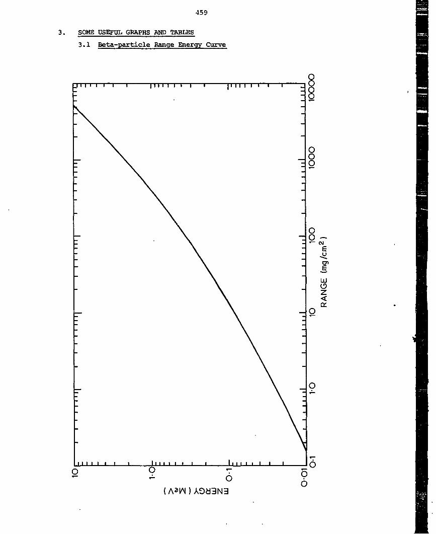
459
3. SOME USEFUL GRAPHS AND TABLES
3.1 Beta-particle Range Energy Carve

460
3.2 Gamma Linear Attenuation Coefficient versus Energy
10'
10
E i
3.
10rl
10'
1 I I I 1 IT
/Uranium (/>=18'75g/cm3)
Lead(p-11-35g/cm3) J
Ordinary concrete (p=2-3g/cm^)
Water (p=1g/cm3)
i i i i i i 111 i i i i i i 111O"1 1
ENERGY, E (MeV)
1O
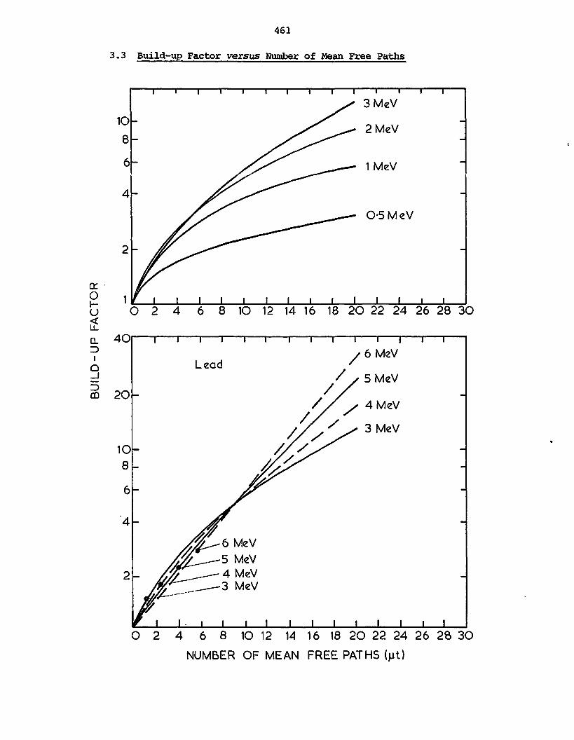
461
3.3 Build-up Factor versus Number of Mean Free Paths
10
8
6
4
ccOi-u
IQ
1
4O
m 2O
108
IMeV
O-5MeV
I IO 2 4 6 8 1O 12 14 16 18 2O 22 24 26 28 3O
T I I T
Lead
•6 MeVMeV
4 MeV-3 MeV
I I J I
O 2 4 6 8 1O 12 14 16 18 2O 22 24 26 26 3O
NUMBER OF MEAN FREE PATHS (jit)

3.4 Half-value Layer versus Photon Energy
A9d3N3 NOlOHd

3.5 Specific Gamma-ray Constants, Gamma Energies and Half-livesfor Some Selected Radionuclides
Nuclide
Americium-241
Barium- 133
Barium- 139
Bromine-82
Caesium- 134m
Caesium-137
Chromium-51
Cobalt-57
Cobalt-60
Copper-64
Gadolinium- 153
Gallium-67
Gold-198
Iodine-125
Iodine-128
Iodine-131
Symbol
2l(1Am95
• 'Ba56
139Bar.f
82Br35
13troCs
137CSbb
51Cr2U
"CO27
*°CO27
M0l29
'««C't
67Ga31
128AU79
125j53
128j53
131X53
Half-life
458 y
10.7 y
83.2 min
35.4 h
2.9 h
30 y
27.8 d
270 d
5.26 y
12.9 h
242 d
78.1 h
2.7 d
60.1 d
25 min
8 d
principal GammaEnergies, MeV(% abundances)
0.060 (36)
0.08 (Jo)0.302 (14)0.356 (69)
0.166 (22.6)
0.55 (72.5)0.62 (40)0.69 (28)0.78 (83.2)0.83 (24)1.04 (28)1.31 (27)1.48 (17)
0.031 (31)U.127 (14)
0.66 (84.6)
0.32 (9.8)
0.014 (9)0.122 (87)0.136 (11)
1.17 (100)1.33 (100)
0.51 (37)0.008 (14)
0.041 (92)0.047 (18)0.097 (30)0.103 (23)
0.09 (40)0.18 (20)0.30 (15)
0.41 (95.5)
0.027 (57)0.031 (10)
0.443 (17.5)
0.364 (82.4)0.637 (7)
Unshielded DoseRate from
1 Ci at 1 m(R h"1)
0.013
0.24
0.02
1.46
0.02
0.31
0.016
0.09
1.33
0.12
0.1
0.1
0.23
0.01
0.04
0.22
Unshielded DoseRate from
1 GBq at 1 ra(pSv h"1)
3.6
65
5.4
394
5.4
83.7
4.3
24
359
32.4
27
27
62
2.7
10.8
59.4
(Continued)

Nuclide
Iridiura-192
Iron-59
MoiKjoiicsu-ju
Mercury-197
Mercury-197m
Mercury-203
Molybdenum-99
Potassium-42
Radium-226
Rubidium-86
Scandium-46
Sodium-24
T@chnetium-99m
Ytterbium-169
Zinc-65
Symbol
192Ir
77
b9pc
26
t r ,..In
2b
'"Kg"0
197m,,80
?(1%g80 •
"MOM2
"2K19
22(>RaBU
ar-Rb37
*6SC21
2"Na11
99">TC
"»3
169yb
70
652n30
Half-life
74 d
45 d
-.55 a
.64.1 h
23.8 h
46.6 d
66.6 h
12.4 h
1600 y
18.7 d
83.8 d
15.0 h
6.02 h
32.0 d
243.8 d
Principal GammaEnergies, MeV
(% abundances)
0.30 (60)O.M C«l)0.32 (86)0.47 (51)
1.1 (56)1.29 (44)
J.33 (2J)1.81 (30)2.1 (15)
0.067 (20)0.069 (36)0.077 (32)
0.134 (30)
0.279 (81.5)
0.14 (5)0.018 (9.8)0.74 (13)0.78 (4.7)
1.52 (18)
See Uranium/Radium (4n+2)Series
1.07 (8.8)
0.880 (100)1.123 (100)
1.37 (100)2.75 (100)
0.14 (85)
0.0635 (85)0.110 (18)0.131 (11)0.177 (22)0.198 (40)0.308 (10)
1.115 (50.7)0.511 (from
6+)
Unshielded DoseRate from
1 Ci at 1 m(R h'1)
0.48
0.64
C« £'
0.04
0.02
0.12
0.15
0.14
0.825
0.05
1.09
2.18
0.07
0.11
0.30
Unshielded DoseRate from
1 GBq at 1 m(pSv h'1)
130
173
243
10.8
5.4
32.4
40.5
37.8
223
13.5
294
589
18.9
29.7
81

465
3.6 Neutron Dose and Dose Rates for Particular Neutron Energies
NeutronEnergyMeV
Thermal
0.0001
0.005
0.02
0.1
0.5
1.0
2.5
5.0
7.5
10
QualityFactor
3
2
2.5
5
8
10
10.5
8
7
7
6.5
Time Ave. Flux(n cm" 2 s" * )
2 2.5 mrem h~ 1
670
500
570
280
80
30
18
20
18
17
17
IntegratedFlux (n cm"2)
= 1 rem
9.6 x io8
7.2 x io8
8.15 x io8
4.08 x 10⁸
1.2 x 10⁸
4.32 x 10⁷
2.64 x 10⁷
2.88 x 10 7
2.64.x 107
2.40 x 10⁷
2.40 x 10⁷
NOTE that the neutron dose depends on neutron energy and neutron
flux.
3.7 Characteristics of Some Radioactive Neutron Sources
Source
2l|1Am-Be
2b2cf
21uPo-Be
238pu_Be
239Pu-Be
226Ra-Be
Reaction
a, n
Spontaneousfission
o, n
a, n
a, n
a, n
Half-life
458 y
2.65 y
138 d
86 y
24 360 y
1620 y
Average NeutronEnergy , MeV
4.5
2.35
4.2
4.5
4.0
4.0
Yield per Ci,neutrons s~ *
2.2 x 10⁶
4.3 x 10⁹
2.5 x 10⁶
2.3 x 10⁶
2.2 x 10⁶
1.3 x 10⁷
Gamma Dose Rateper 106 n s"1
(mR h" l at 1 m)
1
< 1
0.04
< 1
5
60

466
4. HEALTH PHYSICS MONITORING PROGRAM CONSIDERATIONS
When considering a monitoring program each facility must be con-
sidered individually on its merits, taking the following into account:
(i) the type of ionising radiation likely to be encountered;
(ii) the type and degree of shielding provided to minimise external
radiation exposure to personnel;
(iii) the type of containment provided for work with unsealed
radioactive materials and the radioactivity of these materials;
(iv) the type of work to be carried out (e.g. research, routine or
production);
(v) the safety features of the working area (e.g. ventilation,
working surfaces); and
(vi) the training and experience of the staff working in the area.
A monitoring program may include:
(a) monitoring the workplace for external radiation (e.g. dose-
rate meter);
(b) monitoring personnel for external radiation (e.g. film badge);
(c) monitoring working surfaces, floors, walls, machines, etc.
for surface contamination (e.g. contamination monitor);
(d) monitoring skin and clothing of personnel for contamination
(e.g. hand and clothing monitor);
(e) monitoring air in working area for contamination (e.g. air
sampler);
(f) monitoring waste (liquid, solid, gaseous); and !
(g) special monitoring for a particular operation (e.g. during j
maintenance, repair, etc.) in high dose rate areas.
5. ACCIDENTS WITH RADIOACTIVE MATERIALS
Prime objectives following an accident are:
(i) to minimise the exposure of persons to ionising radi-
ations and radioactive materials; and
(ii) to return conditions to normal as soon as possible.
Where necessary the following should be implemented:
(a) evacuate area;
(b) set up barriers, restrict access to area;
(c) measure radiation and contamination levels to determine
the hazard and delineate the accident area;
(d) use suitable protective clothing (e.g. overshoes, boots,
respirators);

467
(e) carry out decontamination;
(f) return radioactive sources to shielding;
(g) monitor persons involved in accident; and
(h) monitor clean up personnel.
Personnel dosemeters should be used during all clean-up operations
where external radiation is present and care taken to minimise hazards
to persons engaged in these operations.
6. PERSONNEL DECONTAMINATION
When a person becomes contaminated, every effort must be made to
remove the contamination as soon as possible. Persistent skin contamin-
ation should be referred to qualified medical staff for treatment.
Simple soap and water washes are often effective if applied as soon
as possible after occurrence of contamination.
For more stubborn contamination, a 1 per cent Cetavlon solution may
be applied followed by washing or a 2 per cent potassium permanganate
solution applied and left for about one minute; hands are then washed
thoroughly and decolourised with 5 per cent sodium metabisulphite sol-
ution.
If at any time during decontamination the skin shows signs of
cracking or becoming red-raw, medical attention should be sought.
7. LICENSING
In most countries users of radioactive materials and devices which
emit ionising radiations are required to have a licence which controls
their use, storage, transport and disposal.
8. TRANSPORT OF RADIOACTIVE MATERIAL
The 1973 IAEA Transport Regulations form the basis of most arrange-
ments for the safe transport of radioactive materials throughout the
world. (Note: This discussion covers the subject briefly; for firm
information refer to the IAEA Transport Regulations.)
There are four basic requirements for packages containing radio-
active materials:
(a) Adequate containment of radioactive material.
(b) Adequate shielding against radiation emitted by the material.
(c) The dissipation of heat generated by high-activity radioactive
material.
(d) Prevention of nuclear criticality when the material is fissile.
Containment
The toxicity of radionuclides varies by a factor of about 108, so

468
there is clearly a need for a number of packaging standards,. Packages
have therefore been divided into five main types: Type A, Type B, low
specific activity, low level solid, and exempt.
Type A packaging is designed to withstand the normal transport
conditions. In an accident, however, it is accepted that the contain-
ment may be breached and that some of the contents may escape. The
maximum activity of each radionuclide which can be transported in a Type
A package is therefore limited so that, in the event of an accident, the
risk to transport workers and members of the public will not be un-
acceptable.
Type A packaging must be capable of passing a series of prescribed
tests which are intended to simulate the damage caused by driving rain
and minor mishaps that would be encountered during rough handling of
packages under normal transport conditions. The tests include a water
spray test, a free drop test, a compression test and a penetration test.
Type A packaging for liquid or gaseous materials, which are more dis-
persible than solids, must be capable of passing additional tests in-
cluding a 9 metre drop.test.
Type B packaging is intended to retain adequate containment and
shielding, even in the event of a severe accident such as a drop while
loading, a vehicle or ship collision, derailment followed by impact with
a bridge or other abutment, or an air to ground crash. There is there-
fore no regulatory upper limit for the activity which can be transported
in a suitably designed Type B package.
Type B packaging must be capable of passing the Type A tests and,
in addition, mechanical tests in which a specimen package is dropped
onto a flat target from a height of 9 metres and then dropped onto the
end of a circular metal bar from a height of one metre, followed by a
thermal test in which the specimen is exposed to a temperature of 800°C
for 30 minutes. A separate specimen must also be capable of passing a
water immersion test in which the specimen is immersed under a head of
water of at least 15 metres for a period of not less than eight hours.
The design, and in some cases the shipment, of Type B packages
requires the approval of the national competent authority because of the
greater .potential hazard of such packages compared with Type A packages.
Type B packages are subdivided into two groups, Type B(U) and Type B(M),
depending on whether the package design warrants the approval of all
competent authorities en route, i.e. Type B Multilateral, or whether the
approval of the competent authority of the country of origin can reasonably
469
be held to be binding on others, i.e. Type B Unilateral.
Type B(U) packages must meet a series of design criteria as speci-
fied in the IAEA Transport Regulations and must also require no opera-
tional controls during transport. Approval of the design of Type B(U)
packages by the competent authority of the country of origin only is
required. Type B(M) packages on the other hand do not meet all the
above design criteria, or else require operational controls during
transport. Approval of the design of Type B(M) packages, and for cer-
tain large shipments approval of the shipment, by the competent author-
ities of the country of origin and of all countries through or into
which the package will be transported, is required.
Low specific activity materials are materials which are regarded as
inherently safe because their specific activity is so low that it is
considered inconceivable that, under any circumstances arising in trans-
port, a sufficient mass of material could be taken into the body to give
rise to a significant radiation dose. Uranium and thorium ores and
their concentrates are an example of low specific activity materials.
These materials can be transported either in bulk as a full load, or in
commercial packages which meet less stringent requirements than those
for Type A packages.
Lou level solid radioactive materials represent an extension of the
low specific activity material concept to include certain types of
consignments of low and medium level radioactive wastes. Such materials
are not inherently safe and so must be transported in strong industrial
packaging under full load conditions.
Exempt items consist of small quantities of radioactive materials,
such as samples and radioactive components of instruments, and articles
which have a low potential hazard. These items are free from most
regulatory requirements.
Shielding
All packages are classified into three categories based on the
external radiation at the surface of the package and at a distance of 1
metre from the surface. The radiation level at a distance of 1 metre
from the surface of the package is referred to as the transport index.
The three categories are as follows:
Category I - : Radiation level at surface < 0.5 mR h"1 and
White package not Fissile Class II or Class III.

470
Category II -
Yellow
Category III -
Yellow
Radiation level at surface between 0.5 and
50 mR h"1, transport index < 1.0, and
package not Fissile Class III.
Radiation level at surface between 50 and
200 mR h"1 and transport index < 10.
The above surface radiation levels have been adopted on the basis
of safe operating experience. The level of 0.5 mR h"1 for Category I -
White packages for example was determined on the basis that an exposure
of 10 mR is the maximum that could be accepted for undeveloped photo-
graphic film. It has been assumed that 24 hours would be the longest
period for which boxes of such film would be close to packages of radio-
active material during transport. Category I - White packages can
therefore be handled and transported with no requirements for segre-
gation from persons or film.
The above radiation categories are identified with three defined
labels as illustrated in the IAEA Transport Regulations. On the Cate-
gory II - Yellow and Category III - Yellow labels it is important that
the transport index be inserted on the label. The transport index is
used to control the number of packages which can be grouped together in
order to ensure that the external radiation level from a group of pack-
ages does not exceed safe levels and also as a criticality control
device.
Higher external radiation levels, up to 1000 mR h"1 in some circum-
stances, are allowable on the external surface of a package when it is
transported under full load conditions, i.e. for a load from a single
consignor having the sole use of a vehicle and in respect of which all
initial, intermediate and final loading and unloading is carried out in
accordance with the directions of the consignor or consignee.
Similar provisions also exist for identifying freight containers
with Category I - White, Category II - Yellow and Category III - Yellow
labels.
9. BIBLIOGRAPHY
Button, J.C.E. [no date] - ASNT Radioisotope Course for Non-Graduates:
Radiation Protection Notes. Australian School of Nuclear Tech-
nology, Lucas Heights (available on request).
Dhew [1970] - Radiological Health Handbook. US Dept. of Health,
Education and Welfare, Washington, DC.
IAEA [1970] - Neutron Moisture Gauges; A Guide-book on Theory and
Practice, IAEA Technical Report Series No. 112.

471
ICRP [1966] - Recommendations of the International Commission on
Radiological Protection (adopted September 1965). ICRP Publication
9, Pergamon, Oxford.
ICRP [1973] - Data for Protection against Ionising Radiation from
External Sources: Supplement to ICRP Publication 14. ICRP Pub-
lication 21, Pergamon, Oxford.
ICRP [1977] - Recommendation of the International Commission on
Radiological Protection. ICRP Publication 26, Pergamon, Oxford.
Radioactive Substances Advisory Committee [1971] - Handbook of Radio-
logical Protection. Part 1 - Data. HMSO, London.