AD-A271 316 (INaval Research Laboratory I%0IF illll lJIiill11! 111 ljWashington, DC 20375-5000

NRL Memorandum Report 6771

Reception of Signals From A Distant TransmittingHalf-Wave Dipole Excited by a Single-Cycle Sinusoid

S. N. SAMADDAR

Radar Analysis Branch

Radar Division

February 18, 1991

'.DTICF UT

93-24704

9 3 1 0 1 8 0 0 2 !Approved for public release; distribution unlimited.

to.rA AppRoveREPORT DOCUMENTATION PAGEN

P•I3•Ic te•omlnq burdlen lot tt,,ý (Ollem'on of -flortm~lon .ý e•t,matr-o to 4Pa-&9 I r,-( pe, espoms -luo-g• the lot• ,- -9 ~ -e'• e ti~~lOn, *s rc~~ .. l'stn• data) W."es

gathefong #"•: m/a-ungjn~ the data ne.•efl anid cOmp~let-9Q and e-•e-9• the (Oiir¢i,0n of infoim ;i~On %endt (o-4?nl% rr9'&rd,,,9 th,% bu;Oe. e•l,"te 0, any other &,p" o 0t h,,

caliea4o5 O verlooo41kO Aveinue,•uggestlOt Ing Rhe•pot6den to w77,ilOn Heaotluaei Se-ce% Ueit-te for information Operaions an Repor%. 11 jefle'wnOav1"1Heghwly SjuV Ie 1104 AVI thnqt() V A 12202.43102 and t IO !he 011.(e of M anaqeeme~ and• 6.9l,~~ PapeI. ro~lt Re'.tj<no. P Io •e• (070A-0168) vV•h,94/,~lon J( 20%01

1. AGENCY USE ONLY (Leave blank) 2 REPORT DATE 3. REEPORT TYPE AND OATES COVERED11991 February. 18 Interim

4. TITLE AND SUBTITLE SA FUNDING NUMBERS

Reception of Signals from a Distant Transmitting 6211N1Half-Wave Dipole Excited by a Sinle-Cncle Sinusoid

6. AUTHOR(S)PM A N

S. N. SAMADDAR

7. PERFORMING ORGANIZATION NAME(S) AND ADDRESSNES) 1. PERFORMING ORGANIZATIONREPORT NUMBER

Naval Research Laboratory NRL Memorandum

4555 Overlook Avenue, SW Report 6771Washington, DC 20375-5000

9. SPONSORING/ MONITORING AGENCY NAME(S) AND ADDRESStES) 10. SPONSORING/ MONITORINGAGENCY REPORT NUMBER

Office of Naval Technology RAteAI2Arlington, Va 22217-5000

11. SUPPLEMENTARY NOTES

12a. DISTRIBUTION /AVAILABILITY STATEMENT 12b. DIS.. iBUTION CODE

Approved for public release; distribution unlimited.

13. ABSTRACT (Maximum 200 words)

Characteristics of the time-dependent received voltage across the terminals of a thin dipolesituated in the radiation zone of a thin transmitting dipole excited by a single-cycle sinusoidal voltageare investigated. In order to study this problem analytically, the zero-order approximate solution forthe currents along the antennas in the frequency domain is used. Each of the four distinct incidentelectric field pulses induces four distinct (although overlapping) voltage pulses through the discon-tinuities of the receiving dipole antenna. When these two dipoles are mutually at the broadside of theother, the time duration of the incident electric field and the induced received voltage are lengthenedby 1.5 cycles and up to 2 cycles respectively. It is observed that the time variation of the induced

received voltage is smoother than the inducing (or incident) electric field. This shows that the receiv-ing dipole behaves like an integrating circuit. Unlike a CW field, the spectrum of a short pulseincident electric field as well as the received voltage have peak values at frequencies higher than thecarrier frequency fo of the exciting single-cycle sinusoid. Both the transmitting and the receivingdipoles attenuate lower frequencies of the spectra of the exciting single-cycle sinusoidal voltage.

14. SUBJECT TERMS 15. NUMBER Of PAGES

Ultra Wideband Antenna 2416- PRICE CODE

17. SECURITY CLASSIFICATION 1B. SECURITY CLASSIFICATION 19. SECURITY CLASSIFICATION 20. LIMITATION OF ABSTRACTOF REPORT OF THIS PAGE OF ABSTRACT

UNCLASSIFIED UNCLASSIFIED UNCLASSIFIED SARNSN 7540-01-280-5500 Standard Form 298 (Rev 2-89)

CONTENTS

1. INTRODUCTION ........................................................................................... 1

2. CHARACTERISTICS OF THE VOLTAGE RECEIVED BY ADIPOLE-DISCUSSION OF RESULTS ............................................................. 3

3. CONCLUSION ............................................................................................... 5

4. APPENDIX - ANALYSIS ................................................................................ 7

5. ACKNOW LEDGMENT .................................................................................... 17

6. REFERENCES ............................................................................................... 17

locesston For

JNTT6 (i-A&IDTIC TABOneannou ed 5]

Ji u..

I D T I C i a'.. -....

iii,

RECEPTION OF SIGNALS FROM A DISTANT TRANSMITTINGHALF-WAVE DIPOLE EXCITED BY A SINGLE-CYCLE SINUSOID

I. INTRODUCTION

In a previous work [Il we studied the behavior of the radiated electric field from a thin half-

wave dipole in free space, excited by a single-cycle sinusoidal voltage with angular carrier frequency

(00. This was investigated analytically by using an approximation, which consists of retaining only

the zero-order solution for the current along the antenna in the frequency domain. This model of a

transmitting dipole and its associated input impedance, which are based on zero-order approximation

of the current without incorporating any radiation damping, was also considered by Franceschetti and

Papas [2]. This model appears to be adequate as long as the observation point is far away from a thin

transmitting dipole. It was shown in [I] that for a suitably matched dipole, the time-dependent radi-

ated electric field was made up of five overlapping pulses indicating that radiation took place only

from the discontinuities of the dipole antenna. In addition, it was found that both the current and the

radiated electric field were extended in time due to the reflection of the current from the end points of

the dipole. The spectral bandwidth of the radiated electric field was narrower than that of the excit-

ing voltage pulse. On observing such characteristics of the radiation of a pulse form a transmitting

dipole antenna, a question then naturally arises, "What will be the behavior of the voltage received

by a similar receiving dipole, upon which the above-mentioned radiated field is incident?" The

present work is devolted to answer that question using similar assumptions and approximations made

in Ref. [1].

Figure 1 shows the geometry of the problem under study. The transmitting dipole AOB of

length 2h, oriented along the z-axis of a coordinate system (x, y, z), is excited at its center 0 (which

is also the origin of this coordinate system) by a single-cycle sinusoidal voltage V0 sin (001 of duration

T. A receiving dipole Ar PB, of length 21 is placed along the z, -axis of another rectangular

Manuscript approved October 5. 1990

coordinate system (xr, yr,zr). the center of the receiving dipole P (r0 , 0o, o0), which is the origin

of the coordinate system (xr,,Yr, Zr), is in the far field of the transmitting dipole AOB with

IOPI = ro. The orientation of the receiving dipole can also be specified by two angles ) and ý,

where X is the angle between PAr and the z-axis, and ;4 is the angle between the x-axis and the pro-

jection of PAr in the x -y plane. If one wishes, one may introduce the Eulerian angles to relate the

two coordinate systems (x, y, z) and (Xr, Yr, Zr).

The problem is at first formulated in the frequency domain subject to the approximations men-

tioned above. To obtain the time dependent received voltage, the inverse Laplace transform is used

with s = io, where s and wo are the Laplace and the Fourier transform variables, respectively. This

transform method is based on the assumption that the computed frequency response of the system is

valid for all frequencies. However, this is not true always, especially when approximations are used

in obtaining the frequency response. Therefore, the time domain result obtained in this way is not

exact. Nevertheless, the present result which can be interpreted readily exhibits the dominant

mechanisms of radiation and reception by a dipole.

It is found that each incident signal, which is radiated by the transmitting dipole, induces five

signals at the receiving input terminals via five different paths. Since two of these signals look alike,

because they have the same phase, only four distinct overlapping signals are induced at the center ter-

minals of the receiving dipole antenna. It may be recalled [1] that the transmitted electric field also

consists of five overlapping signals, two of which have the same phase, and thus showing four distinct

radiated pulses. These phenomena show again that the mechanism of both the radiation and reception

of electromagnetic pulses by dipoles is governed by the respective discontinuities. Among other

characteristics of the received voltage, it is interesting to note that in order to receive the maximum

energy from such radiated pulses, the receiver must be tuned at a frequency about 25% higher than

the carrier frequency fo of the single-cycle exciting sinusoidal voltage. This is a sharp departure

2

from the tuning requirement for the reception of CW signals. Detailed discussions of numerical

results and theoretical analysis are presented in separate sections.

2. CHARACTERISTICS OF THE VOLTAGE RECEIVED BY A DIPOLE - DISCUSSION

OF RESULTS

Figure 1 shows a receiving dipole ArPBr in the far field of a transmitting dipole antenna AOB

excited by a single-cycle sinusoidal voltage V0 sin wot (where wo = 27r fo). Thc voltage VL is meas-

ured across a load impedance ZL which connects the input terminals at the center of the receiving

dipole. Since it is assumed that ZL is real and independent of frequency, the behavior of the received

antenna current and the received voltage is identical. It is found in Ref. [1], that at a distant point, P,

in absence of the receiving antenna, the radiated field arrives from five different paths immediately

after the transmitted antenna is excited at its feed point 0. These paths are (Fig. 1)

OP, OAP, OBP OAOP and OBOP. The phases of the signals represented by paths OAOP and

OBOP are the same. Therefore, an observer at P will see only four distinct overlapping signals.

However, when a receiving dipole is placed with its center at P, each of the pulses (or signals)

represented by the five paths mentioned above, will induce voltage pulses at the center of the receiv-

ing dipole in five different ways, since each arriving or incident signal does not necessarily take a sin-

gle path for inducing voltage at the center of the receiving antenna respectively. For example, the

incident signal represented by the path OAP will enter at P of the receiving dipole ArPBr via five dif-

ferent paths, namely, OAP, OAAP, OABrP, OAPAP and OAPBrP, before the corresponding vol-

tages are induced at P. Since the paths PArP and PBrP are equal, the phases of the induced signals

represented by OAPArP and OAPBP are the same. Therefore, the signal which radiates from the

point A of the transmitting dipole induces four distinct voltage pulses at the center of the receiving

dipole. In this way one finds (Eqs. 16 and 241 that the induced voltage at the center of the receiving

dipole consists of sixteen overlapping distinct signals. When the receiving dipole, instead of being

3

oriented arbitrarily with fespect to he transmitting dipole, is placed at the broadside ot the transmit-

ting antenna, the abovementioned sixteen distinct voltage signals reduce to nine.

In Fig. 2 the normalized time-dependent broadside radiated electric field

Eo(ro, 00 = r/2, t)/[V0o 0 /(41rZoro)1, in the absence of or before being disturbed by the presence of

the receiving dipole, is shown (dotted curve) as a function of a normalized time t*fo, where

t* = t - ro/c is the retarded time. Along with this radiated electric field, the normalized induced

timc-zlcpendent load voltage VL (ro, 00, Or, t)/[V0o(230 r0 f•J across the terminals of the receiving

dipole, which is placed at the broadside (00 = 7r/2 = Or) of the transmitting dipole, is also shown

(solid curve) as a function of the normalized time t*fo. In this case the lengths of the transmitting

and the receiving dipoles are half-wave at the carrier frequency fo, i.e., h = I = 0.25c/fo. Since

this induced voltage and the incident (or radiated) electric field are normalized differently, their

amplitudes should not be compared. Only their shapes as functions of the normalized time t*fo may

be of interest. Figure 2 shows that for a single-cycle sinusoidal exciting voltage (o0 T = 21r), the

radiated electric field before being received by the receiving antenna is extended in time to 1.5 cycles,

whereas the duration of the induced load voltage across the terminals of the receiving antenna is

increased to 2 cycles when h = 2. The increase of the time duration of the radiated (or incident) sig-

nal is caused by the reflections of the induced current from the ends of the transmitting antenna. On

the other hand, the additional time extension of the received voltage pulse is caused by the reflection

of the incident electric field from the ends of the receiving antenna. It is interesting to note that the

received voltage pulse has a smoother shape than that of the incident electric field. This observation

suggests that during the process of reception of the incident field, the receiving antenna integrates the

incoming signal in some sense. In other words, the receiving antenna acts like an integrating circuit.

This is true and can be supported theoretically (see Eq. 24).

Figure 3 shows, using a given set of values of h and I that when the length of the receiving

dipole is shorter than the half-wave transmitting dipole (I < h), the duration of the received voltage

4

will be between 1.5 to 2 cycles. It may then be inferred that the duration of the received voltage

pulse may exced 2-cycles, if the receiving antenna is made longer than 2h. In Fig. 4 a normalized

spectrum of the received voltage I 30r0 V (to) I (see Eq. 27), as well as the spectrum of the exciting

single-cycle sinusoidal voltage with different normalization, are presented as functions of the normal-

ized frequency f/fo. Because of different normalizations, their amplitudes should not be compared.

This figure reveals another interesting charac.teristic of the received voltage pulse, when the

transmitter is excited by a single-cycle sinusoidal voltage with carrier frequency f 0 = w0/2wr. The

maximum energy in the received voltage is delivered at a frequency about 25% higher than fo.

Therefore, the receiver should be tuned at about 1.25 fo. This phenomenon shows a sharp departure

from the tuning requirement for the reception of CW signals. It is also shown in Ref. f1] that the

peak value of the spectrum of the radiated electric field from a transmitting dipole occurs at a fre-

quency f > fo. However, if the number of cycles in the exciting sinusoid is increased, the value f of

the peak of the spectrum of the radiated field, approaches fo gradually 1]. Consequently, it is

expected that the spectrum of the received voltage will also show a similar behavior.

3. CONCLUSION

Characteristics of the received time-dependent voltage across the terminals at the center of a

receiving dipole placed in the radiation zone of a transmitting dipole, excited by a single-cycle

sinusoidal voltage are studied. The behavior of the corresponding radiated electric field from the

transmitting dipole excited in the same manner was investigated previously [Ref. 11. It is o" served

that the radiated electric field consists of four distinct overlapping pulses with an extended duration of

1.5 cycles. This increase in pulse length is caused by the reflections of current from from the end-

points of the transmitting half-wave dipole. Each of these four radiated pulses then induces four dis-

tinct voltage pulses across the terminals of the receiving dipole. The process of reception of the

5

incoming radiated field undergoes through reflections form the end points of the receiving antenna as

the induced current travels along the latter. This mechanism causes additional increase of time dura-

tion so that the total duration is between 1.5 and 2 cycles of the received signal, depending on tne

length of the receiving dipole compared relative to that of the half-wave transmitter. It is also

observed that both the processes of radiation from and reception by a dipole antenna take place via

the respective discontinuities of the dipole concerned. The receiving antenna behaves like an integrat-

ing circuit so far as the incoming field is concerned. Since the spectra of both the radiated and

received signals have peaks at a frequency higher than the carrier frequency fo of the exciting

sinusoidal voltage, the receiving antenna should be tuned to a frequency higher (about 25%) than fo.

However, if the number of cycles in the exciting sinusoid is increased, the peak of the received spec-

trum approaches fo. This phenomenon may be viewed as if the receiving dipole is filtering out lower

frequencies further during the reception of short pulses.

6

APPENDIX

4. ANALYS:S

Consider a thin linear receiving dipole antenna of length 21 situated in an arbitrary manner [Fig.

11 in the far field of a distant transmitting half-wave dipole of length 2h, excited at its center bN a

single-cycle sinusoidal voltage Vo sin w0t. The transmitting dipole antenna lies along the z-axis of the

coordinate system x, y, z; whereas the receiving dipole is oriented along the zr-axis of the coordinate

system Xr, yr Zr. The centers of these antennas separated by a very large distance ro are at the ori-

gins of the respective coordinate systems. It will be assumed that the direction cosines of the axes

X,,, Yr, Zr, with respect to the coordinate system x, y, z are known.

Our objective here is to calculate the open circuit induced voltage across the input terminals of

the receiving dipole upon which the radiated field from the transmitting antenna is incident. From

this result the voltage across a receiving load impedance ZL can be determined easily. At first, the

problem will be formulated in the frequency domain. Then the corresponding time domain result will

be obtained by an application of the Fourier or Laplace transform. In this analysis we shall resort to

the same kind of approximation, namely, the use of zero-order current distribution along the thin

receiving dipole, as done for the transmitting dipole [1]. With this background in mind, let us assume

that an electromagnetic field, represented by its electric vector Ei (r0 , 0o, 0o, w), in the frequency

domain, is incident upon a receiving dipole, the center of which is located at (ro, 00, •0). The coor-

dinates (r0 , 00, 00) are assigned with respect to the transmitting dipole. Then an open circuit voltage

i'c(Or, Obr; ro, 0o, 0o; w), which we shall simply write as Vo(W) for convenience, will be induced

across the terminals of the receiving dipole. The spherical angles (Or, Or), measured with respect to

the receiving antenna, refer to the direction of the wave vector of the incident field as seen by an

observer at the receiving antenna. It may be noted that the angles (0o, 0o) define the same direction

as observed from the transmitting site. The induced open curcuit voltage V0,(w) then can be

expressed in the following way [3, 41.

7

V,(t) = E(ro0, Oo ; ' O) - -hr(O,, c,;r LO), (1)

where the veLor effective height h,(O,, 0•, w) of the receiving antenna is defined by

hr(Or, to, w) = [1 -I I 7, r(r, W)exp i- (r ) dv, C_• C

In the above relation (2), the subscript r refers to the receiving antenna respectively. For example, r,

and 7 r designate a unit vector in a radial direction and the position vector of a source element meas-

ured from the coordinate system of the receiving antenna. 1 is a unit dyadic. Jr(rr, wo) and I,,, are

the induced current density and input current of the receiving antenna respectively. When the receiv-

ing dipole is along the Zr-axis, we have

sinO, 1 (-3)hr(Or, Or, W) = hr(Or, W) Or I I(: LhH.ZrcosOi d-r,(

where kr is the unit vector in the Or-direction. For the zero-order approximation of the induced

current, the above expression becomes [11

2 Cos coSO - cos VZ 1hr(Or, -o =-Or c IIr(4)

hrOn./c) sinOr " sin(wi/c)

In view of the reciprocity theorem, the vector effective height of the transmitting dipole antenna

of length 2h and radiating in the 00-direction can be expressed in the following manner.

2 Cos [ - cos0o] - cos wh I

To',Oo W)• = -Oo0 I (5)(W•/C) sinO0 • sin(wh/c)

where Oo is a unit vector in the 00-,irection. Incidentally, it may be noted that the incident field

Ei(ro, 00; 0o, w), which is the radiated electric field from the transmitting dipole antenna, can be

expressed in terms of the transmitter effective height h,(OO,w,) in the following way 11, 31.

8

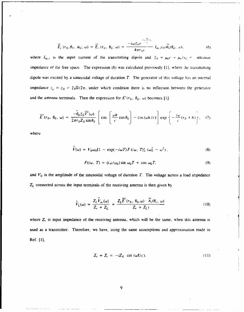
E, (ro0 Oo, 0o, wA) = E, (ro, 00" ) = !,rrc I6,(wh,(O, ').6

where li,., is the input current of the transmitting dipole and ý' = c= p/cc = intiInsic

impedance of the free space. The expression (6) was calculated previously [11, where ýhe transmitting

dipole was excited by a sinusoidal voltage of duration T. The generator of this voltage has an internal

impedance z. zo = 0 0o/21r, under which condition there is no reflection between the generator

and the antenna terminals. Then the expression for EV(ro, 06, w) becomes 1I]

E(ro, 00, o) = 2 Or cos F- cos0o cos(wh/c)1 exp (. + h 7

'2.rrZr sin 00 L C(7)

where

V(w) = Voo0[I - exp(-iwT)F(iw, T)],(wo - ) (8)

F(iw, 7) = (iwl/,o) sin woT + cos woT, (9)

and Vo is the amplitude of the sinusoidal voltage of duration T. The voltage across a load impedance

ZL connected across the input terminals of the receiving antenna is then given by

-~ ZL VC(W) _ZLE(ro, 0 00W) hrT(Or. W)(0Zr +ZL Zr + ZL)

where Z, is input impedance of the receiving antenna, which will be the same, when this antenna is

used as a transmitter. Therefore, we have, using the same assumptions and approximation made in

Ref. (11,

Zr = Z' = -iZo cot (wI/c). (11)

9

Then taking ZL = Zg = Z 0, the expression (10) can be rewritten in the following way, where

use has been niade of equations (4) and (7)-(9) with iw = s.

V/L(-is) = G( 00oro, 00, 0,) 4w 2 le -SrF.(s,7_- 11 [cosh f1- cos0 - cosh -- 1 (12)0 s(s 2 + W2) C

cosh I cOo cosh ]exps(ro + h + I)/cj,

where 3o = wol/c and s is the Laplace transform variable.

G(/o, ro, 00, Or) = (O O)(13)2(/30 ro) 12 sin 0o sin 0,

Then the time-dependent receiving load voltage is given by the following inverse Laplace transform of

VL (-is).

VL(rO, 00, Or, t*) = ." VL(-is)es ds, (14)

where t* = t - ro/c is the retarded time. It can easily be seen using the L'Hospital's rule that

s = 0 is not a pole of VL(-is). However, it will be necessary to express the hyperbolic cosine func-

tions in terms of exponentials, in which case for an individual term in (12) or (13), s = 0 will

become a pole. Therefore, the contour F in (14) is chosen along the imaginary axis of the complex

s-plane with indentations from the right side at the poles s = 0 and s = -- iwo0 . Finally, the contour

is closed by a semi-circle in the left-half plane at infinity, so that the poles lie inside this closed con-

tour. Then the time-dependent load voltage VL(ro, 00, Or, t*) can be expressed in the following

form.

VL(ro, 00, Or, t*) = G(o0 ro, 00, Or) S(Oo, Or,t*), (15)

where S(Oo, Or, t*) is the Laplace transform of VL(ro, 0o, 0, t*)/ G(3oro, 0o,00).

10

The time function S(o0, Ot, t*) consists of twenty-five signals, each of which has time duration

T and appears at different overlapping time intervals. Since some signals have the same phases, there

are only sixteen distinct signals Assuming that T = nTo, where n is a positive integer and

To = I1/fo = a period of a single-cycle, the function S(Oo, O, t*) can be represented in terms of

unit step functions U(ti) and U(t, - T). with i = I to 16.

S(0 0 , O, 1'*) = [cos WotI - 11 [U(tI) - U(tI -- T)]

+ [cos (oot 2 ) - II [U(t2 ) - U(t, - T)]

- [cos (oo13) -1] [U(13) - U(t 3 -T)] - [cos (w014) - lI[U(t 4 ) - U(t 4 - T)]

- [cos (oot 5 ) -1] WUO 5 ) - U(t 5 -7)] + [cos (toot6) - l1[U(t 6 ) -U6 - T)]

- [cos (WOt7) -1] U(t 7 ) - U(t 7 - T)] - [cos (Lot 8) - 1][U(t8) - U(I 8 - T)] (16)

- 1cos (W019) -11 [U(tg) - U(t 9 - T)] - [cos (tot 1o) - 1[U(t to) - U(t - T)]

+ [cos (Wto01) -11 WU0 11) -U0 - ) - [cos (t0t112) - 1J[U(t 1 2 ) - U(t 1 2 - T)]

+ [cos (WOt 13) - 1] [U(t 13) - 3- T)I - [cos (WOot 14) - 11 [Ut 14) - U(t 14 - T)7

- [cos (Got 15) - 11 [U(t 15) - U15 D + Icos (Wt 16) -- 1 [U(t 16) - U( 16 - T)I

Each of the quantities t I, t.... t 16, defined below, represents the respective time taken by an indi-

vidual signa] to travel from the input terminals of the transmitting dipole to those of the receiving

dipole via various discontinuities (input and end-points) of both antennas [Fig. 11.

=t* = t - ro/c = retarded time associated with the travel time along the pathOP, (17a)

11

(17b)

t2 = 11 - 21/c = retarded time associated with the travel time along each of the paths, OPArP and

OPBrP, for which the phases are the same. This shows that the second term of (16) is contributed by

these two paths equally.

(17c)

t3 = tI - I(I - COS Or)/C = retarded time associated with the travel time along the path OArP,

(17d)

14 = t I - 1( + Cs Or)/C = retarded time associated with the travel time along the path OBrP.

(18a)

t5 = tI - h(I - cos 00)1c = retarded time associated with the time along the path OAP,

(18b)

16 = tI - h(l - cos 60)/C - 1(1 - cos Or/c = retarded time associated with the travel time

along the path OAAr

(18c)

17 = tI - h(1 - cos 00)/C - (1 + cos Or)/c = retarded time associated with the travel time

along the path OABrP

(18d)

t8 = t - h(1 - cos 00)/c - 21/c = retarded time associated with the travel time along each of

the paths OAPArP and OAPBrP. This means that the 8dh term of (16) is contributed equally by these

two paths.

(19a)

t9 = I- h(l + cos 00)/c = retarded time associated with the travel time along the path OBP,

(19b)

t10= t - h(l + cos 00)/c- I(1 + cos Or)/C = retarded time associated with the travel time

along the path OBBrP.

12

(19c)

= I - h(l + cos 00 )/c - (I - cos O,)/c = retarded time associated with the travel time

along the pain OBArP,

(19d)

t12 1 - h(I + cos 00)/c - 21/c = retarded time associated with the travel time along each of

the paths, OBPArP and OBPBrP. Therefore, the 12th term of (16) is contributed equally by these

two paths.

(20a)

113 = t] - 2h/c = retarded time associated with the travel time along each of the paths. OAOP

and OBOP. This Ž. ws that the 13th term of (16) is equally contributed by these two paths.

(20b)

t14 = tI - 2h Ic - I(1 - cos Or)/c = retarded time associated with the travel time along each of

the paths OAOArP and OBPBrP. Therefore, the 140 term of (16) is equally contributed by these two

paths.

(20c)

t1 5 = I - 2h/c - I(1 + cos 0r)Ic = retarded time associated with the travel time along each of

the paths, OAOBP and OBOBrP. Therefore, the 15th term of (16) is equally contributed by these two

paths.

(20d)

t16 = t1 - 2h Ic - 21/c = retarded time associated with the travel time along each of the paths,

OAOPArP, OAOPBrP, OBOPArP and OBOPBrP. Therefore, the last term of (16) is equally contri-

buted by these four paths.

It is interesting to notice that in the absence of the receiving dipole, the four distinct signals

which would have radiated from the transmitting dipole to a distant point P can be identified with the

13

terms associated with the travel times t , 15, tq and 113, respectively. Each of these four signals then

induces four distinct voltage pulses at the terminals of the receiving dipole. It should be understood

that the signals associated with the travel times t,, t5, 19 and 113, repectively, also constitute a

portion of the total induced voltage pulse when the receiving dipole is present.

When the receiving and the transmitting dipoles are at the broadside of each other, i.e., %khen

00 = 7r/2 = 0 r, one finds that t3 = t4 = 11 - 1/C, t5 = 19 = t -- h/c, t6 = t7 = t10 =

tI1 =t - h/c - 1c, t8 = t12 = tj-h/c - 21/c and 114 =115 =tl - 2h/c - 1/c. There-

fore, the sixteen distinct signals given by Eq (16), reduce to nine distinct signals.

The result (16) is obtained from (14) via residue calculus. It can also be extracted from (14) by

using some theorems associated with the Laplace transform. In particular the following relations are

found to be helpful.

L-[exp I-sti) - L(g(t)j] = g(t - ti) - U(t - ti) (21a)

L - t exp I-s(ti + 731 - Ljg(t + 7)1] = g - ti) - 1t - 7) (21b)

L[IU(t - ti) - U(t -i - T)7] - 0 g(r)d T (21c)

S+ T T(/s) S eSt g( - ti) dt - (I/s) exp I-s(t, + 73) 0o g (r) dr.

where the symbols L and L- stand for the Laplace transform operation and its inverse respectively.

I, g(-r - ti) U( - ti) - U(r - t - 7)] dT

=[U(t - ti) - U(t -t - 7)] •- 1 ' g(T - ti) dT, (22)

T

provided 0 g(t) dt = 0.

14

Using these relations, which can be established easily, one can then show from equation (14), that

when the exciting voltage is

V(t) = V,(t) . [U(t) - U(t - 7)], (23)

where V,(t) stands for g(t) in the relations (21a) to (22), then

VL(ro, 00, 0r, t*)/[O0 • Or/12(ro/c)Q sin Oo sin 0,11

= - [U( t) - ((t - 7")] '0" V 5(r) dr-[U(t2) - U(t 2 - T)Ijo'ý V,(r) dT

"+ [U(t 3 ) - U(03 - 7)] 0o" V,(r) d + [U(1 4 ) - U( 4 - 0T)]" oV,(r)d

+ [V(t 5 ) - U(05 - 7)] 1ot Vs(7-) d- - [U(t 6) - U0 6 - 7)] • 1J V,(r)di

- [U(tT) - U(t 7 - 0 19' V,(T) dr - [U(ts) - U(ts - T)] • 10" V,(r)dr

+ [U(tg) - UQt - 7)] so11 V1(-r) di - [U(tl0) - U(4to - 7)] " o'° V.(7)dr

- JU(t11 ) - U(tlj - 7)] soI V,(r) dr + [U(t 12) + U(t 12 - 7)] - 0 "' V,(r)d7

-- [U(tl 3 ) - U/3- 7')] 113t, Vs(") di + [U(Q14 ) - UQ1I4 - T')] " o'` V5(i)dr"00

+ [Ut 15) - Ut -1 )] ' "' V,(r) d7 - (U(t16) - U(t16 - T)] 0 '0" V,(r)d7 (24)

The expression (24) shows that the receiving antenna is behaving like an integrating circuit. Simi-

larly, replacing wo by -is in (7) ano th,.n taking its inverse Laplace transform, the time-dependent

radiated electric field can be expressed in the following manner [using 21a and 21b].

Oo - -i(ro, 0o, T)I[ý0 I(4Zo r ro sin Oo)]

= [U(tO) - U0t - 7)] - V5(ti) - [U(t5 ) - U(t 5 - 7)] V 5(t5 ), (25)

15

-- (U(tW - U(19 - 7)1 Vs(t 9 ) + IU(/13) - U(03 - T)] V((tl3).

The correspc,,ding modified zero-order time-dependent antenna current on the transmitting dipole can

also be represented using the same principle.

IOM(Z, t)/(2Z0 )

= [U(t - 1:1/c - u(t- Iz I/c - T)] Vs(t - zI 1/c)

- [Ult - (2h, - I :)/ct - UI(t - (2h - Iz 1)/c - T7] Vs(t - (2h - z1 )/c). (26)

Observing now ihe &i i s between (25) above and (12) of ref. Ill and (26) above and (13) of ref.

[1], the results (25) and (26) can be interpreted in the same manner, i.e., discontinuities of an antenna

play a dominant role in radiation mechanism.

Comparing the expression (7) and (12) with s = iwo, it can be seen that the spectrum of the radi-

ated field from the transmitting dipole is not the same as that of the induced load voltage of the

receiving dipole. The reason for this phenomenon may be explained in the following way. Since

antennas (the transmitting as well as the receiving dipoles) behave like frequency filters, the frequency

spectrum of the incident field is expected to be filtered further by the receiving dipole. We have

already observed [1] that when a single-cycle sinusoidal voltage excites a transmitting dipole, the

spectrum of the radiated field is attenuated as well as filtered.

The expression for the spectrum of the received load voltage when 00 = r/2 = 0 r, i.e., when

both the antennas are mutually at each other's broadside, reduces to the following form (with

Vo = 1).

i iOo0 ,t()[ Two=ro- (1 - cos wohlc) (1 - cos wl/c) •

F~sin IT(w -wo) I sin I T(w +wo) I r sin'[T(w -wo)/21 sin 2 T(c,+ wo)/2t 1>fT(w- w) T(- +wo) J L u - w-)12 +wo0 )12 J27

16

In (27) the quantity in the square bracket multiplied by T represents the spectrum of the exciting

sinusoidal voltage of duration T.

5. ACKNOWLEDGMENT

This problem was suggested by Dr. M.I. Skolnik, with whom the author had several useful dis-

cussions. The author would like to thank Mr. Chester E. Fox, Jr., for providing numerical results.

6. REFERENCES

1. S.N. Samaddar, "Radiated Field From a Thin Half-wave Dipole Excited by a Single-Cycle

Sinusoid," NRL Memorandum Report 6465, Naval Research Laboratory, Washington, DC

20375-5000, October 31, 1989.

2. G. Franceschetti and C.H. Papas, "Pulsed Antennas," IEEE Transactions, AP-22, pp. 651-661,

1974.

3. D.L. Sengupta and C. -T. Tai, "Radiation and Reception of Transients by Linear Antennas,"

Chapter 4, pp. 181-235, in Transient Electromagnetic Fields, ed. by L.B. Felsen, Springer-

Verlag, Berlin, Heidelberg, New York, 1976.

4. R.E. Collin, "The Receiving Antenna," Chapter 4, pp. 93-137, in Antenna Theory - Part 1,

ed. by R.E. Collin and F.J. Zucker, McGraw-Hill Book Co., New York, 1969.

17

z

-j0 IZWyW

>1LL Cl) z (!

< F-

>lI E O

LLJ->

a- W L-

0

to 0

(v\ N zw E!

-x < - I

-~ co

-- 0

18

4NORMAUZED

3 RECEIVED VOLTAGE

NORMAUZED INCIDENT h=t. =0.25 f,/c

ELECTRIC FIELD / 7 /2=Er

2 AT THE RECEIVING

ANTENNA

11

0

S~THERE•FORE, ONLY

Sj ~THE SHAPES

- 3 - j MAY BE OF INTEREST.\

COMPARED- 4 , - I I

0 0.5 1 1.5 2

NORMALIZED TIME t*foFig. 2 -- Normalized Radiated Electric Field and Received voltage when the

Antennas are at Broadside of each other and h = 1

19

S- - 2 -•DIFERENTLY.

3(h/c)f0 = 0.25(L/c) f-0= 0.21

2 0= -Tr2

LU

00 0

UJ

CC" -2

-3

-4,

0 0.4 0.8 1.0 1.2 1.6 2

NORMALIZED TIME t*foFig. 3 - Normalized Received voltage when I < h and the Antennas are at

Broadside of each other

20

7 Th, EXCITING VOLTAGE SPECTRUM

1-- RECEIVED VOLTAGE SPECTRUM

0.8 I /2 = E)

Sl THESE TWO ARE NORMAUZED

- j DIFFERENTLY. THEREFORE ONLY

SII THE SHAPES MAY BE OF INTERESTIJ 0.6 I THEIR AMPUTUDE SHOULD

c/) NOT BE COMPARED.

ujIN 0

I.-Io 10.1

z -%

0

0 0.5 1 1.5 2 2.5 3 3.5 4 4.5 5

NORMALIZED FREQUENCY f/fo

Fig. 4 - Normalized Exciting voltage and Received voltage spectra

21