AD-AO81 608 NAVAL POSTGRADUATE SCHOOL MONTEREY CA F/B I /I

ON THE COMPUTATIONAL COMPLEXITY OF BRANCH AND BOUND SEARCH STRA-ETC(U)NOV 79 0 R SMITH NSFMCS74-14445

UNCLASSIFIEQ NPS52-79-004 NL

I 2 ff l f II

IIIIIIIIIIIIII...fIIEEEEE-EIEEEItEEEEEEEEI-EEII-EEE--EE-IIIEIIEEIIIIIIII

NPS 52-79-004

NAVAL POSTGRADUATE SCHOOLMonterey, California

IELECTE nS MAI~A U.96A .-

On the Computational Complexity

of Branch and Bound Search Strategies

by

Douglas R. Smith

November 1979

Approved for public release; distribution unlimited.

Prepared for:National Science FoundationWashington, D. C. 20550

80 :3 10,, .,..,"

NAVAL POSTGRADUATE SCHOOLMonterey, California

Rear Admiral T. F. Dedman Jack R. BorstingSuperintendent Provost

This research was partially supported by the NationalScience Foundation.

Reproduction of all or part of this report is authorized.

DOUJGLA R.' SMITH

Assistant Professor ofComputer Science

Reviewed b Released by:

H. , irman WILLIAM M. TOLLES,Dept. o Co e cience Dean of Research

I.t

UNCLASSIFIEDSECURITY CLASSIFICATION OF THIS PAGE (llu, Dae Enterd)

REPORT DOCUMENTATION PAGE a CMRLUCTRoSBEFORE COMMLETWG FORM,.m .qRT..NUN . -la 1. GOVT ACCESSION NO: 3. RECIPIENTS CATALOG NUMBER

I:NPS 52-79- L,-TI L (and Subtio T V r I - Vm q..OVENED

Te _mutational q lexity of Branch Technical *OioptoI- 'hd ourSearch Straegies

.... I. PERFORMING ORG. REPORT MUIRa

7. AUTHOR(a) NTA O N

~IDouglas R/ SmithAENDAOS NSF' MCS74-14444AOl

*.PROMNSRGANIZATION NAEADAOE 10. PROGRAM E MNT.-PROjEcT. TASKNaval Postgraduate School /AES UI UURMonterey, CA 93940

I L. CONTROLLING OFFICE NAME AND ADDIRESSV

National Science Foundation 3o 79Washington, D. C. 20550 1 L00 --

14. MONITORING AGENCY NAME & AODRESS(it different from Controllin01 Office) IS. SECURITY CLASS. (of this Wagp)

Unclassified

IS.. OECL ASI FICATIONDOWNGRADINGSCHEDULE

IS. DISTRIBUTION STATEMENT (of this Report)

Approved for Public Release; distribution unlimited

17. DISTRIBUTION STATEMENT (of the abstract entered It Block 20. It different Ifo Rseport)

IS. SUPPLEMENTARY NOTES

1. KEY WORDS (Continue on reverse side It neessary and identity by block numbee)

Combinatorial Optimization Tree SearchBranch and Bound Probabilistic ModellingCmplexity of ComputationSearch Strategy

20. A STRACT (Continue on reverse side It necessary ind Identif by bloek mmber)

'64ny important problems in operations research, artificial intelligence,, and other areas of computer science seem to require search in order to

find an optimal solution. A branch and bound procedure, which imposes atree structure on the search, is often the most efficient known means for

i * solving these problems. While for some branch and bound algorithms a worstcase complexity bound is known, the average case complexity is usuallyunknown despite the fact that it gives more information about the

DD 1.AN75 1473 EDITION OF I NOV .S IS OBSOLETE UNCLASSIFIED

S/N 0102-014- 601 SECURITY CLASEIFICATION OF THIS PAGE (IO D#e ntered)

i '

NCLASSZFIDW_.U4ITY CLASSIFICATION OF THIS PAOfIQbhm Data emA0

N!

\

performance of the algorithm. In this dissertation the branch and boundmethod is discussed and a probabilistic model of its domain is given,namely a class of trees with an associated probability measure. The best-bound-first search strategy and depth-first search strategy are discussedand results on the expected time and space complexity of these strategiesare presented and discussed. The best-bound-first search strategy is shownto be optimal in both time and space. These results are illustrated by datafrom randomly generated traveling salesman problems. Evidence is presentedwhich suggelts that the assymetric traveling salesma problem can be solvedin time O(n ln2 (n)) on the average.

I.!9

UNCLASSIFIEDSECURITY CLASSIFICATION OF THIS PAOIfIIYen Data n.rtd)

Accession r

i .Just ificto

Dist special

n r

and bound procedure, which imposes a tree structure on the

search, is often the most efficient known means for solving these

problems. While for some branch and bound algorithms a worst

case complexity bound is known, the average case complexity isusually unknown despite the fact that it gives more information

about the performance of the algorithm. In this dissertation thebranch and bound method is discussed and a probabilistic model of

its domain is given, namely a class of trees with an associated

probability measure. The best bound first and depth-first search

strategies are discussed and results on the expected time and

space complexity of these strategies are presented and compared.

The best-bound search strategy is shown to be optimal in both

time and space. These results are illustrated by data from ran-dom traveling salesman problems. Evidence is presented which

suggests that the assymetric traveling salesman problem can beasolved exactly in time O(n31n2 (n)) on the average.

I.

r

abu th pefrac-o h lith.Ihiiisrtto-h

brnhadbudmto sdsusdadapoaiitcmdlo

TABLE OF CONTENTS

PageLIST OF FIGURES . . . . . . . . . . . . . . . . . . . . . . v

LIST OF TABLES . . . . . . . . . . .. . . . . . . . . vi

ACKNOWLaEDGEMENTS . . . . . . . . . . .. . . . . . . . . .* vii

1. INTRODUCTION . . . . . . . . . . . .. .. .. ... . . 1

2. BRANCH AND BOUND ALGORITHMS . . . .. .. .. ... . . 9

3. A MODEL OF BRANCH AND BOUND SEARCH TREES .... . . . . 29

6. HEURISTIC SEARCH STRATEGIES . . . ..... . . . . . . 41

5. THE BEST-BOUND-FIRST SEARCH STRATEGY . .. .. . .. . 50 s

6. THE DEPTH-FIRST SEARCH STRATEGY . ..... . . . . . . 55

7. AN APPLICATION TO THE TRAVELING SALESMAN PROBLEM ... . 71

8. CONCLUSIONS . .. .. .. ... . .. .. .. .. .. .. .. 86

APPENDIX . . . . . . . . . . . . . . . . . . . . . .. . . 89

LIST OF REFERENCES..................... . . 95

r LIST OF FIGURES

Figure Page

2.1 Application of the branching rule to FS . . . . ... . . 12

S2.2 A branch and procedure . . . . . . . . . . . . . . . . 15

2.3 A Search Tree and the Order in which Several Search

Strategies Examine the Nodes ......... . ... 17

2.4 A and Ab in Case 2 ... ............... 22

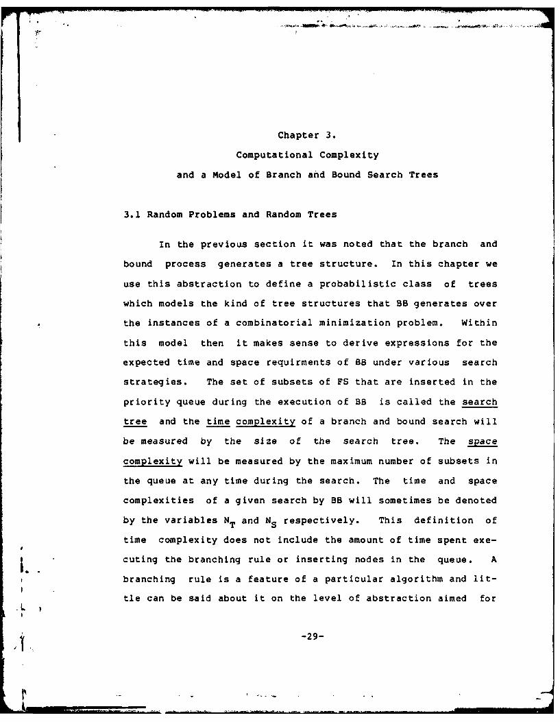
3.1 An arc-labelled tree . . . . . . . . . . . . . . . . . 28

3.2 Generating a Random Arc-Labelled Tree . . . . . . . . . 28

3.3 A Treetop and a Branch . . . . . . . . . . . . . . . . 33

3.4 8(i) for (pl0 ,Ql00)-Trees . . . . . . . . . . . . . . . 34

3.5 DEP(m) for (P10,Q100)-Trees . . . . . . . . . . . . . . 35

6.1 A Treetop . . . . . . . . . . . . .................... 52

6.2 The Structure of a Depth-First Search Tree . . . . .. 58

6.3 Formation of an Arbitrary Tree in LTD * * * * * * * * 60

7.1 The data from Table 4 plotted showinfg the growth of the

Mean Search Tree Size as a Function of the Length of the

Leftmost Branch .... ....... . . ... .... 80

A.1 An Algorithm for Computing 8 Given P and Q . . . o . . 86

A.2 An Algorithm for Computing Size(b) . . ........ . 88

IV

lb

I

1'-- -

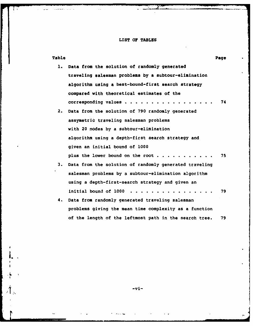
LIST OF TABLES

Table Page

1. Data from the solution of randomly generated

traveling salesman problems by a subtour-elimination

algorithm using a best-bound-first search strategy

compared with theoretical estimates of the

corresponding values . . . . . . . . . . . . . . . . . 74

2. Data from the solution of 790 randomly generated

assymetric traveling salesman problems

with 20 nodes by a subtour-elimination

algorithm using a depth-first search strategy and

given an initial bound of 1000

plus the lower bound on the root ......... . . . . 75

3. Data from the solution of randomly generated traveling

salesman problems by a subtour-elimination algorithm

using a depth-first-search strategy and given an

initial bound of 1000 . .................. 79

4. Data from randomly generated traveling salesman

problems giving the mean time complexity as a function

of the length of the leftmost path in the search tree. 79

I.

j, -vi-

2 -

ACKNOWLEDGEMENTS

I am indebted to Prof. Alan Biermann fbr his support, con-

stant encouragement, and advice which always seemed to be on tar-

get. I would also like to thank Prof. Kishor Trivedi who sug-

gested several key ideas in chapter 4. I am grateful to my wife,

Carol, who helped me out in many ways during the course of this

work. This dissertation was partially supported by NSF Grant

MCS74-14445-AO1.

..h

-vii-

Chapter 1.

Introduction

By an instance of a combinatorial problem we mean the

problem of finding a constructive proof of

ax P(x) for xeFs (1)

where FS is a discrete set of objects and P is a predicate de-

fined on FS. That is, we want to find an object in FS which

has the property P. In many cases it is not the truth but

rather the feasibility of a constructive proof of (1) which is

in doubt. Some combinatorial problems require all solutions

which satisfy (1). We restrict ourselves to the problem of

finding a single solution, but note that all results obtained

in this case can be extended to handle this slighty harder

problem. There are countless examples which satisfy (1) rang-

ing from easy problems like sorting (find a permutation of an

input list which is sorted), to more difficult problems like

integer programming (find an vector of integers which satisfies

a set of constraints) and theorem proving (find a proof se-

quence for a statement in some language by means of a given set

of axioms and rules of inference).

Generally when we speak of a combinatorial problem, we

mean a set C of related instances of the form (1). These in-

stances can be classified according to their size, enabling us

to speak of a problem instance of size n. The question of what

the size of an instance is and how to encode problem instances

can be tricky. See [Aho, Hopcroft and Ullman 1974] for a

disscusion of encodings in the context of the class of problems

called P and NP. For our purposes we will say that a measure

of the size of a problem instance has the property that all

problem instances with the same size have the same feasible set

FS. For example in an instance of the sorting problem, we are

given a vector of n numbers. Here n is taken as the size of

the instance and the feasible set is the set of permutations of

n objects. The predicate P(x) tests whether a permutation x

applied to the given vector results in a sorted vector. In an

instance of an integer programming problem, we are given a set

of constraints on n variables. n is taken as the instance size

and the feasible set is the set of all integer vectors of

length n. In theorem proving we are given a statement and take

its length as the size of the instance. Here the feasible set

is the set of all legal proof sequences in the theory. If P

contains an optimization clause then (1) is called a

combinatorial optimization problem. In this dissertation we

will be particularly interested in combinatorial minimization

problems in which we seek a constructive proof of

3x[P(x) &Vy[P(y) => f(x)<f(y)] ] for xyeFS (2)I.where f, called the objective function, maps FS into the nonne-

gative reals.

-2-

,\

-, . -. ", . -- -*

Some combinatorial problems can be solved directly; i.e.

the solution is reached by a straightforward construction with

no backtracking. When no direct constructive method is known,

there are three principal search methods for finding solutions

to combinatorial problems called enumerative search, local

search and global search. In an enumerative search the objects

of FS are produced one at a time and tested. The search ter-

minates the first time that P is satisfied. If we are seeking

an optimal object then FS must be exhaustively searched and FS

must be finite in order to assure termination. Some problems

such as that of finding a key in an unordered list require

enumerative search. Local search (Reiter and Sherman 1965; Lin

1965; Weiner, Savage, and Bagchi 1973; Papadimitriou and

Steiglitz 1977] is usually applied to combinatorial optimiza-

tion problems and is characterized by a topology or neighbor-

hood structure imposed on the set of objects FS. For any ob-

ject in the set we can readily find all of its neighbors. A

search proceeds by selecting some initial object, picking a

neighbor which satisfies P and betters the value of the objec-

tive function, then picking a neighbor of the neighbor and so

on, until an object is found which is optimal with respect to

all of its neighbors. This object is called a local optimum.

If the neighborhood structure is exact (a local optimum is a

global optimum) then the search can terminate on the first lo-

L. cal optimum found. For many problems it is difficult to find

or infeasible to use an exact neighborhood structure and so a

neighborhood structure with many local optima is used. For ex-

-3-

- II II I I

ample it has been shown (Weiner, Savage and Bagchi 1973] that

in a exact neighborhood structure for the traveling salesman

problem on n cities each object (a cyclic permutation of the n

cities) must have at least (n-2)1/2 neighbors therefore render-

ing exact local search infeasible. If many local optima exist

then the best we can do is to restart the search at a new ini-

tial object, eventually obtaining a set of local optima from

which the best may be picked. These local search methods are

analogous to the descent and gradient methods of mathematical

programming [Luenberger 1973). On complex spaces this method

is best suited for finding approximate solutions, i.e. objects

which are nearly optimal but not neccesarily optimal.

A global search is characterized by the handling of sets

of objects rather than single objects at a time as in local

search. A powerful form of global search may be described as

follows. The problem again is to find an object in a set FS

which satisfies P. If such an object cannot be found easily

then we generate a set of subproblems by splitting FS into sub-

sets. The i th subproblem has the form,

3x P(x) xeFS i CFS (3)

where U FSi = FS. This process of creating subproblems byi

means of splitting the feasible set is repeated until a solu-

tion is found in one of the subsets (which may not occur until

the sets are reduced to singleton sets). A global search is

Ithe essence of the well-known backtrack technique (Lehmer 1958;

Golumb and Baumert 1965, Knuth 1974] of which branch and bound

is a special case. Another kind of global search which is re-

-4-

/'i ..

lated to branch and bound is the well-known technique of dynam-

ic programming [Bellman 1957; Morin and Marsten 1976, 1978;

Ibaraki 1978].

The question of whether search is the most efficient

method for solving some combinatorial problems is a deep one

which might be specialized in the well-known P-NP question

[Cook 1971;Karp 1972]. Problems which can be solved directly

tend to have fast algorithms which run in polynomial time in

the problem size. On the other hand search algorithms for a

problem tend to have a worst-case running time which includes

as a factor the size of FS, the feasible set. The NP-complete

problems are a class of problems for which either all or none

are solvable by algorithms which run in time given by a polyno-

mial of the problem size. Since the size of the search space

FS of the NP-complete problems is superpolynomial (usually ei-

ther exponential or factorial), and all known deterministic al-

gorithms for NP-complete problems have superpolynomial worst-

case time bounds, one might conjecture that the P-NP question

is equivalent to the question of whether NP-complete problems

require search for their solution. At present global search

algorithms of the branch and bound variety are the most effi-

cient known methods for solving NP-hard problems. It may be

that in answering the P=NP? question wholly new solution

methods will be found which obviate the need for search. How-

ever the complexity of some global search algorithms is our

best current estimate of the intrinsic complexity of a wide

Arange of important combinatorial problems.

-5-T1

The complexity of a global search algorithm has usually

been measured by its worst case behavior over all instances of

a problem, i.e. an upper bound on its performance. The obvious

problem with such a measure is that it gives little information

about the usual or average performance of the algorithm. For

example recently [Klee and minty 1970] some examples have been

found which cause the simplex algorithm for solving linear pro-

grams to run in exponential time, yet its usual performance is

so good that it is one of the most widely used computer algo-

rithms. It is especially true of global search algorithms

which can have widely varying behaviors over the set of in-

stances of a problem that the average case complexity gives

more information than a worst-case measure about the perfor-

mance of the algorithm.

Branch and bound is a global search technique applicable

to combinatorial minimization problems. In the past decade

branch and bound seems to have emerged as the principal method

for solving problems of this type which have no direct solu-

tion. Just a few of the applications of the branch and bound

method include integer programming (Garfinkel and Nemhauser

1972], flow shop and job shop sequencing [Ignall and Schrage

1965], traveling salesman problems (Bellmore and Nemhauser

1968; Bellmore and Malone 1972], heuristic search in the form

of the Aalgorithm [Hart, Nilsson, and Raphael 1968; Nilsson

19721, and pattern recognition (Kanal 1978]. The alpha-beta

technique used in game playing is an extension of branch and

bound to the game tree environment (Knuth and Moore 1975].

-6-

-M~~ Irq

Branch and bound algorithms can be roughly classified

into two kinds according to properties of the trees they gen-

erate. In the first kind, solutions to the problem only occur

at or below some fixed depth in the tree depending on the prob-

lem size. In this approach a solution is built up a component

at a time until a complete object is created. In the second

kind of algorithm a solution may be found at any depth of the

tree (including the possibility that the solution is found at

the root). Relaxation procedures fall in this category. In a

relaxation procedure a relaxed version of the problem is solved

at each node of the tree. In a relaxation of a combinatorial

problem of the form (1) we want a constructive proof of

-3x PWx for xeFS' (4)

where FSCFS'. This approach may be useful if there is a fast

algorithm for solving (4). If the relaxed solution is also a

solution to the restricted problem (the solution is in FS) ,

then we're done, otherwise the relaxed solution is used to

create subproblems by splitting FS' into subsets in such a way

that the relaxed solution is precluded from further considera-

tion. The i th subproblem has the form

ax P(x) xeFS' iCFS I. (5)

where FSCMU FS' 1 CFS' (c.f. (3)). It is this second kind ofi

branch and bound algorithm which will be modeled and studied in

this dissertation. This is not to say that the results of the

dissertation do not apply to algorithms of the first kind but

merely that our intent was to study the second kind.

* The purpose of this dissertation is to analyze the branch

-7-

and bound procedure under several search strategies in order to

obtain quantitative estimates of their expected time and space

requirements. The results of this analysis provide a framework

for analyzing and predicting the expected resource requirements

of specific branch and bound algorithms as illustrated in

chapter ~.These results may also be used to compare the rela-

tive efficiency of search strategies.

In chapter 2 the branch and bound algorithm and its

domain are presented and several important properties are

derived. In Chapter 3 our model of branch and bound search

trees is introduced and properties of the model trees are

derived. Also the sense in which we will use the term complex-

ity is developed and discussed. Chapter 4 develops results on

the complexity of general search strategies. Chapters 5 and 6

apply these results to the best-bound-first search strategy and

the depth-first search strategy respectively. Also in chapter

6 the expected time complexity of a depth-first search is stu-

died as a function of the depth of the first solution found in

the search tree. Using the results obtained in previous

chapters, a subtour elimination algorithm for the traveling

salesman problem is modeled in chapter 7 and it is suggested

that it has an expected running time of O(n 3 ln 2 (n)). The

reader may wish to reader chapter 7 in parallel with chapters 5

and 6 in order to see an application of the theorems being

developed.

-8-

*44.,

Chapter 2.

Branch and Bound Algorithms

Branch and bound algorithms are designed to solve com-

binatorial minimization problems. We will denote the set of in-

stances of size n of a combinatorial minimization problem by Cn

= (PS nCOSTn) where FSn is a countable set of objects called

the feasible set and COST n is a set of cost functions such that

any cCCOSTn maps FSn into nonnegative integers. The parameter

n of a class C varies over positive integers and is intendedn

as a natural measure of the size of the instances of the prob-

lem. We will assume that the cost functions must satisfy the

condition that no more than a finite number of objects in PS

may have a given cost. A problem instance from Cn has the fol-,

lowing form: Given ceCOSTi, find s CFSn such that for all sCFSn

c(s ) < c(s), i.e. find a least cost object in the feasible

set. In the following discussion we will omit the subscript on

FS and COST when no confusion can arise. The idea of a branch

and bound search is to split FS into subsets and to compute a

lower bound on the cost of the objects within each subset.

Those subsets whose bound exceeds the cost of some known

j(perhaps nonoptimal) solution can be discarded since they can-

not contain an optimal solution. The remaining subsets are re-

Lpeatedly split and bounded until an object is found whose cost

i * -9-

r . --

+-- + , A.+ . •"

does not exceed the bound on any subset, hence that object is a

minimal cost solution. The special power of the branch and

bound method comes from this ability to prune away whole sets

of objects when they can be shown not to contain an optimal ob-

ject. The choice of which of the currently unexamined subsets

to examine next is specified by a search strategy.

We will use the example of the Traveling Salesman Problem

(TSP) throughout this dissertation. The TSP originated with

the problem of finding the shortest route for visiting all of n

cities and returning to the starting point. We will deal with

the following generalization of the TSP of size n. Given a

complete directed graph with n nodes and arc weights given by

an nxn cost matrix, find the least cost hamiltonian cycle (a

cycle which passes once through each node of the graph).

Clearly the set of hamiltonian cycles on a complete directed

graph is isomorphic to the set of cyclic permutations of n ob-

jects. Here the feasible set is the set of all hamiltonian cy-

cles on a complete directed graph of n nodes (or cyclic permu-

tations). The cost functions are a set of cost matrices which

specify the arc weights. The cost of a hamiltonian cycle is

the sum of the weights on the arcs of the cycle. If C=[ci,j]

is a cost matrix, then ci,j is the weight on the directed arc

from node i to j. We do not require that c, j = cj, i . There

is a long history of attempts to devise efficient algorithms

for solving traveling salesman problems. At present the most

efficient algorithms for solving TSPs make use of a relaxation

procedure embedded in a branch and bound algorithm. The Held

j++ -10-

'k

and Karp (Held and Karp 19711 algorithm for solving symmetric

TSPs (the cost matrix is required to be symmetric) makes use of

a relaxation based on minimum spanning trees. The most effi-

cient known approach to solving assymetric TSPs makes us. of a

relaxation which allows all permutations to be feasible rather

than just cyclic permutations. This relaxed problem Is known

as the Assignment Problem.

A branch and bound algorithm has three major components.

A branching rule B is a rule determining if and how a subset of

FS is to be split into subsets. If the least cost object in a

subset can be extracted easily then the branching rule does not

split the subset. Otherwise the subset is split into a .inite

number of proper subsets which then represent smaller and

therefore easier subproblems to solve. Note that the repeated

application of the branching rule generates a tree structure as

in figure 2.1. The branching rule for a branch and bound algo-

rithm employing a relaxation procedure is slightly different

from branching rules for ordinary branch and bound algorithms.

Given a set S, in the latter case U B(S) - S, and in the former

case U B(S)C S since we preclude some of the relaxed feasible

objects. The branching rule of course does not split a single-

ton set since the least cost object (namely the only object) in

the set can be easily extracted. It will be useful to define

* the function parent as follows: if SleB(S) for some S SFS then

I.-parent(S 1 )iS.The second component of a branch and bound algorithm is a

Figure 2.1. Application of the branching rule to FS.

B(FS) - {S1 S 2 ,S3)

where SlCFS, S 3 -FS,

and S1 uS 2 US3 gPS.

lower bound function which maps subsets of FS into nonnegative

integers. Intuitively the lower bound function computes a

lower bound on the cost of all objects in a given subset of FS.

Formally LB must satisfy the following conditions:

1. for SUFS and seS LB(S)<c(s)

(LB computes a lower bound on the cost of objects in S),

2. for SisSaFS LB(S.)< LB(S i )

(the lower bound values increase monotonically on any path

from the root in the tree),

3. if B(S) = S (B does not split S) then LB(S) = c(s*), where

s is the least cost object in S

(when the least cost object in a set can be extracted, the

cost of that object is the lower bound value of the set).

The lower bound function is used to eliminate from con-

sideration those subsets of FS which can be shown not to con-

tain the least cost solution. If it is known that a least cost

object has a cost of at most cI then any subset S for which

LB(S)>c I cannot yield the optimal solution.

-12-/1 '

I'f =m , '- .. . . . . .-II-

The third component of a branch and bound algorithm is a

search strategy which is a rule for choosing to which of the

currently active subsets of FS the branching rule should be ap-

plied .For conceptual simplicity and uniformity of notation,

a search strategy will be realized here by a heuristic function

h:2FS->PRIORITY where PRIORITY is a set which depends on the

particular search strategy. Of those subsets waiting to be ex-

plo~red via the branching rule we choose that subset S with the

smallest heuristic value h(S). At any particular time during a

branch and bound search, a certain set of subsets are waiting

to have the branching rule applied to them. If the heuristic

value of these subsets (computed by h) are distinct for all

such times during a search of any problem in any class then the

heuristic function is called unambiguous. Some common search

strategies will be discussed below along with unambiguous

heuristic functions which realize them.

The branch and bound algorithm for finding a single least

cost object is given below in an ad-hoc ALGOL-like language.

The principal data structure employed is a priority queue. A

priority queue used here is a data structure which stores data

objects (in this case nodes representing subsets of FS) with an

associated priority given by the heuristic function h. The

queue is accessible only by the functions NONEMPTY, which re-

turns true if and only if the queue is nonempty, REMOVETOP,

I.. which removes and returns the data object in the queue of

highest priority (priority i is higher than priority j if and

only if 1<j for a suitable definition of the relation <h) and

-13-

INSERT which inserts a data object into the queue with its as-

sociated priority. Efficient algorithms for manipulating

priority queues in this manner are discussed in [Aho, Hopcroft,

and Ullman 1974]. The )rocedure BB in figure 2.2 is typically

invoked with the node representing PS and ca as arguments. In

later 'iscussion of BB we will use the node symbol No to

represent .. An obvious improvement of BB is to check that

cost(Ni)<bound in statement 10 before the node Ni is inserted

in the queue. While such a test will improve the performance

of BB somewhat in practice, we omit it here for the sake of

simplifying our analysis of the behavior of BB. Its inclusion

would not affect our order of magnitude results on the time

complexity of branch and bound search but would have the effect

of lowering the space complexity somewhat. Several other

enhancements of the pruning power of BB may be added to this

code but they are not always easy to discover for a particular

problem. A dominance relation (Kohler and Steiglitz 1974;

Ibaraki 1977, 1978] is a relation on subsets of FS such that if

S1 dominates S2 then S2 cannot contain a better solution than

S1 , so S2 can be eliminated. This test is a direct generaliza-

tion of the lower bound test. If it can be determined that two

subsets SIS 2 SFS are equivalent in the sense that the optimal

solution in one is as good as the optimal solution in the oth-

er, then only one of these subsets needs to be explored. This

test is called an equivalence test [Ibaraki 1977, 1978].

I." One focus of this dissertation is on several common

search strategies and the effect they have on the average case

-14-

1I - - ! - _!! ! !. . .. . . ... . . . I

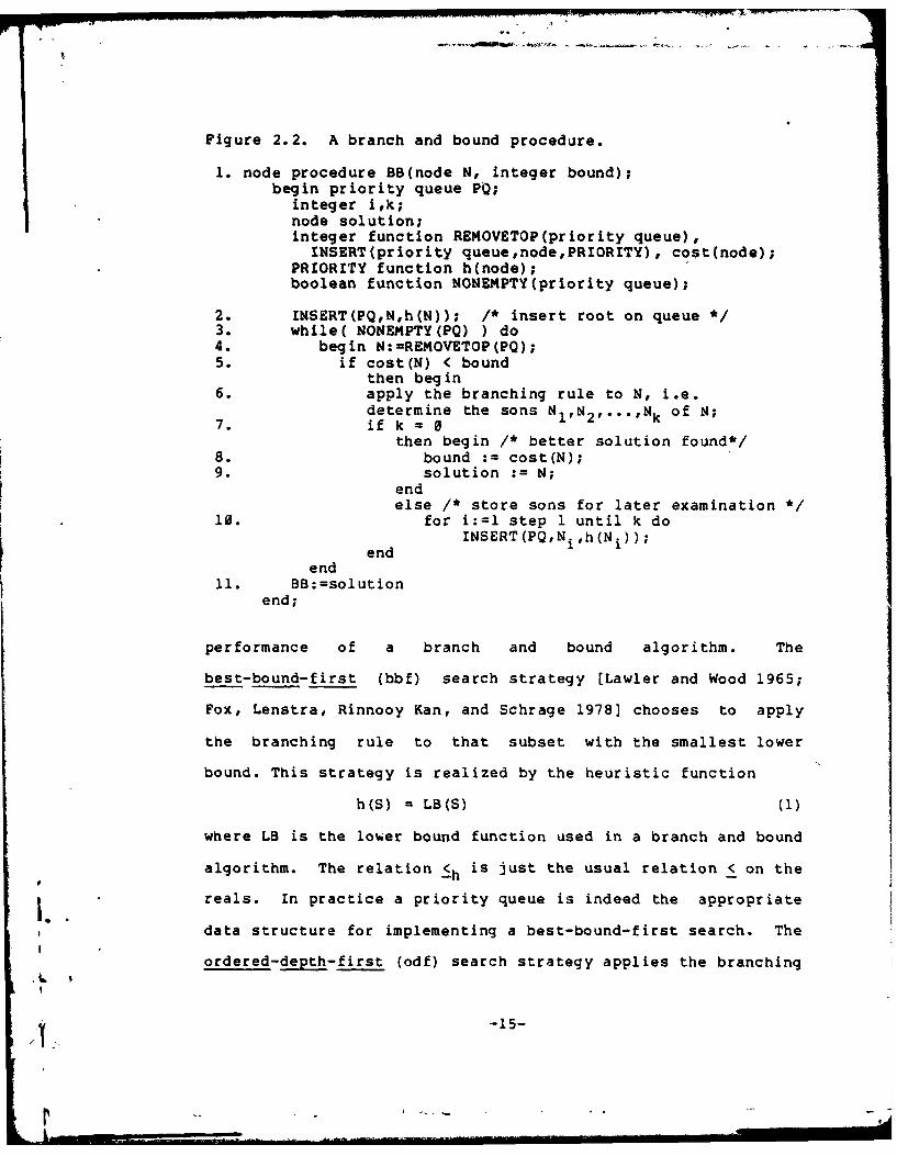
Figure 2.2. A branch and bound procedure.

1. node procedure BB(node N, integer bound);begin priority queue PQ;

integer i,k;node solution;integer function REMOVETOP(priority queue),INSERT(priority queue,node,PRIORITY), cost(node);

PRIORITY function h(node);boolean function NONEMPTY(priority queue);

2. INSERT(PQ,N,h(N)); /* insert root on queue */3. while( NONEMPTY(PQ) ) do4. begin N:=REMOVETOP(PQ);5. if cost(N) < bound

then begin6. apply the branching rule to N, i.e.

determine the sons NlN 2 1 ... ,Nk of N;7. if k = 0

then begin /* better solution found*/8. bound := cost(N);9. solution := N;

endelse /* store sons for later examination *1

10. for i:=l step 1 until k doINSERT (PQ,Ni ,h(Ni));

end 1 1end11. B8: =solutionend;

performance of a branch and bound algorithm. The

best-bound-first (bbf) search strategy [Lawler and Wood 1965;

Fox, Lenstra, Rinnooy Kan, and Schrage 1978] chooses to apply

the branching rule to that subset with the smallest lower

bound. This strategy is realized by the heuristic function

h(S) = LB(S) (1)

where LB is the lower bound function used in a branch and bound

algorithm. The relation <h is just the usual relation < on the

1reals. In practice a priority queue is indeed the appropriate

data structure for implementing a best-bound-first search. The

ordered-depth-first (odf) search strategy applies the branching

-15-

I:' I ' .. .".. . ... .... . .. .. .I:

rule to the least cost of the most recently split subsets and

may be realized by

h(S) - (d(S),LB(S)) (2a)

where d(S) - depth of the subset S in the tree generated by SB

and the range of h is the set of ordered pairs. This heuristic

function makes the priority queue simulate a stack each element

of which is a priority queue, which is the way one would imple-

ment this search strategy in practice. The

generation-order-depth-first (godf) search strategy applies the

branching rule to the first generated of the subsets of a split

set and can be realized by

h(S) = (d(S),i) (2b)

for the ith generated set. Again h produces an ordered pair.

This heuristic function makes the priority queue simulate a

stack whose elements are queues (or stacks; it does not

matter). For both of these heuristic functions we define

(a,b)<h(c,d) if and only if a>c or (a=c and b<d), i.e. subset S

has higher priority h(S) = (a,b) than subset T where h(T) -

(c,d) if and only if either S is deeper in the tree or S and T

have the same depth but the lower bound on S is less than the

lower bound on T. The ordered-breadth-first (obf) search stra-

tegy chooses to examine the least cost of the subsets which has

the smallest depth in the tree generated by BB. A particular

heuristic function realization is

h(S) = (d(S),LB(S)) (3a)

as for depth-first search. In practice an ordered-breadth-

first search is implemented using a separate priority queue for

-16-

Ir-

each level of the search tree so that the nodes on a given lev-

el can be extracted in order of increasing cost. Here we de-

fine (a,b)< h(c,d) if and only if a<c or (a=c and b<d). The

generation-order-breadth-first (gobf) search strategy examines

the subsets a level at a time in the order of their generation,

and may be realized by

h(S) = (d(S),i) (3b)

for the it h generated node on level d(S). In practice a

generation-order-breadth-first search may be implemented using

a single queue for storing nodes of the search tree. Note that

according to the realizations given, both ordered-depth-first

search and ordered-breadth-first search have local best-bound

search components. E.g. in a breadth-first search a best-bound

search is performed on the set of nodes that appear at a given

depth. Figure 2.3 gives an example of a tree and the order in

which each of the above search strategies examines the tree is

given.

As an example of a branch and bound algorithm we will

consider a subtour-elimination algorithm for solving traveling

salesman problems. Subtour-elimination algorithms make use of

a relaxation of the traveling salesman problem called the as-

signment problem (AP) which can be easily solved. The assign-

ment problem comes from the problem of assigning n men to n

jobs in a way which minimizes the cost of the assignment. We

are given an nxn matrix [ci] where c. is the cost of assign-

ing man i to job j. The cost of an assignment is the sum of

the costs of assigning each man to his job. The feasible set

-17-

S-

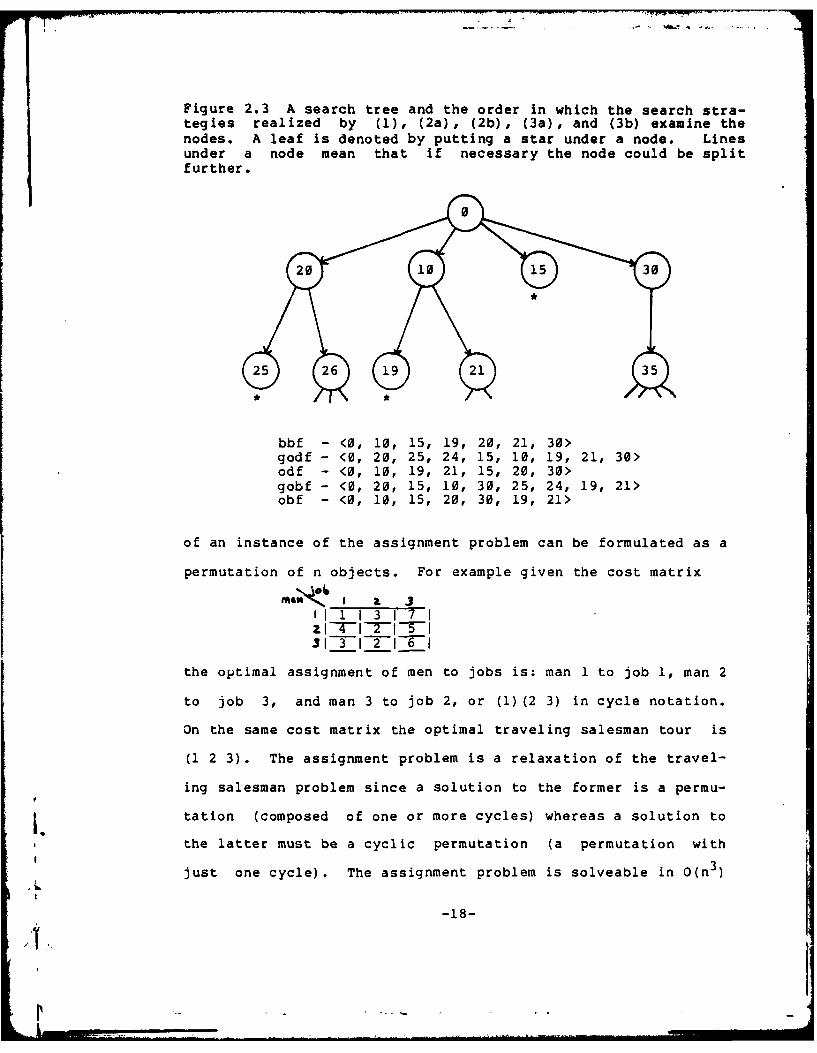
Figure 2.3 A search tree and the order in which the search stra-tegies realized by (1), (2a), (2b), (3a), and (3b) examine thenodes. A leaf is denoted by putting a star under a node. Linesunder a node mean that if necessary the node could be splitfurther.

bb20 <,10 5 19, 20 1 30>

go5 26 <0 1095,2,1,0 9 21, 3

odf - <0, 10, 19, 1, 15, 20, 30>gobf - <0, 20, 15, 10, 30, 25, 24, 21, 21>

gobf - <0, 10, 15, 20, 30, 19, 24,1> ,21

of an instance of the assignment problem can be formulated as a

permutation of n objects. For example given the cost matrix

Ill 13 3

31 3 1 2 16 1

the optimal assignment of men to jobs is: man 1 to job 1, man 2

to job 3, and man 3 to job 2, or (1) (2 3) in cycle notation.

On the same cost matrix the optimal traveling salesman tour is

(1 2 3). The assignment problem is a relaxation of the travel-

ing salesman problem since a solution to the former is a permu-

* I tation (composed of one or more cycles) whereas a solution to

the latter must be a cyclic permutation (a permutation with

just one cycle). The assignment problem is solveable in O(n3

-18-

time for an initial problem and 0(n2) for subsequent modified

versions of the initial problem [Bellmore and Malone 1971;

Lawler 1976]. Subtour-elimination algorithms differ mainly in

their choice of branching rule. The following branching rule

was proposed by Shapiro [Shapiro 1966]:

Given cost matrix C, solve the assignment problem with

respect to C. If the least cost solution, w, is cyclic, then we

have extracted the least cost cyclic permutation over the

feasible set of C, so there is no need to branch. If V is non-

cyclic then pick one of its subcycles, say the smallest, and

let this cycle be denoted (il,i2,...,ik). In the optimal cost

cyclic permutation, at least one of the nodes in this cycle

must be directed outside the cycle since the subcycle cannot be

a part of a cyclic permutation. The feasible set is split asfollos: Inthe.th

follows: In the j tsubset we force the node ij to connect to a

node not in the cycle (i11i2 ,...,ij) by setting the matrix en-

tries

=ci 2 = ... ci k = C"

The lower bound function is simply the cost of the as-

signment problem solution. It is easily shown that this is a

lower bound function. Condition 1 for a lower bound function

(the lower bound function yields a lower bound on the cost of

all objects in a given set), is satisfied since the assignment

solution is by definition a lower bound on the cost of all per-

mutations feasible with respect the cost matrix. Condition 2

(if SisS then the lower bound on Sj is < the lower bound on

-19-

Si) is satisfied because the least cost permutation in a set S

will have at least as small a cost as the least cost permuta-

tion in any subset of S. Condition 3 (if B(S)-(S} then* *

LB(S)-c(s ) where s is the least cost object in S) is satis-

fied since a set S is not split if the assignment solution is

also a traveling salesman solution. In this case the lower

bound is just the cost of the least cost feasible object (a cy-

clic permutation) in S. There are a number of variations on

the branching rule given in [Bellmore and Nemhauser 1971; Gar-

finkel 1973; Smith, Srinivasan, and Thompson 1977].

In all published versions the smallest subcycle of the

assignment solution is chosen to guide the set splitting. This

is justifiable on the general principle of tree searching that

if possible it is wise to arrange the tree such that smaller

branching factors are near the top of the tree and larger

branching factors are deeper in the tree. The reason behind

this principle is that if a node is pruned near the top of such

a tree, there is a relatively larger reduction in the size of

the feasible space due to the fact that the feasible space has

been split fewer times by the smaller branching factor

[Reingold, Neivergelt and Deo 1977, pages 111-112]. The choice

of the smallest subcycle is good from another point of view.

Bellmore and Malone (Bellmore and Malone 1971] have shown that

this choice maximizes the reduction in the the number of feasi-

ble noncyclic solutions.

i.The subtour-elimination approach first appeared in [East-

-20-

I'-

man 19571 and was subsequently developed by (Shapiro 1966;

Bellmore and Malone 1971; Smith, Srinivasan, and Thompson

1977].

Some Properties of Branch and Bound Algorithms

Efforts have been made to devise a formalism general

enough to cover the diverse applications of the branch and

bound procedure (Lawler and Wood 1966; Mitten 1970; Rinnooy Kan

1974, 1976; Kohler and Steiglitz 1974; Ibaraki 1976, 1978].

These formalisms have been used to prove correctness and termi-

nation properties and also to investigate theoretically the ef-

fects of various choices of parameters on performance.

Although the theorems in this section are not essentially new

the proofs are new in order to cover our different definitions

and assumptions.

The first proposition allows us to assume that the

heuristic realizations of the search strategies considered

above are unambiguous.

Proposition 2.1: The best-bound-first, depth-first (both or-

dered and generation-order) , and breadth-first (both ordered

and generation-order) search strategies can be realized by

unambiguous heuristic functions.

Proof: We can show that (1), (2a), and (3a) are unambigu-

ous if the lower bound function LB satisfies the following con-

-21-

dition: for any S, T_9FS if S#T then LB(S)#LB(T). If for a

particular problem and branch and bound algorithm LB does not

satisfy this condition then a new lower bound function can be

constructed at runtime as follows: LB'(S) = (LB(S),k) where S

is the kth distinct subset of FS with cost LB(S) examined to

the current point in the search. With regards to the relation

< used in line 5 of figure 2.2, define (a,b)<(c,d) if and only

if a<c or (a-c and b<d). Clearly LB' generates distinct bounds

on distinct subsets. The heuristic function for best-bound-

first search (1) h(S)-LB'(S) is unambiguous since all values of

h for distinct subsets are distinct. The same reasoning holds

for (2) and (3) since the range of h incorporates the lower

bound LB'.

Let us now consider generation-order-depth-first search.

Suppose there is a tree such that at some time during a

generation-order-depth-first search there are distinct subsets

S1 and S2 in memory with the same heuristic value h(S1 ) =

h(S2). Thus d(S1 ) = d(S2 ) and i = iS where d(S) = depth of2 1 2s i1 2

S and is is the generation number of S. S1 and S2 clearly can-

not have the same parent set otherwise they would not have the

same generation number. Suppose now without loss of generality

that Sl was generated prior to S2. Let P2 denote the parent of

S2. We have d(P2) = d(S2)-l. Since S1 is generated prior to

S2 and there is a time when both Sl and S2 are in memory simul-

taneously, Si must be on the queue when P2 is split to form S2

and its sibling sets. But P2 cannot be chosen over Sl for

branching because d(P2)<d(Sl) and therefore h(P2)>h(Sl). This-

-22-/I -

L r',m- ....

! '"' '- . .. ..... . . .a a a I , I ... .... . , . . . . - . . -. ., , . . '

contradiction shows that there cannot be two distinct sets on

the queue with the same heuristic value under generation-

order-depth-first search. A gobf is unambiguous because no two

sets on a given level can be assigned the same generation

number, so all assigned priorities are distinct. QED

The following sequence of definitions together with pro-

position 2.1 and lemma 2.1 lead up to a theorem regarding the

conditions under which BB will find an optimal solution to an

instance of a combinatorial minimization problem. Let A denote

the sequence of nodes examined by BB'(N,,oo) where BB' is BB

with the test of statement 5 replaced by the value TRUE. Thus

A is the order in which BB examines the entire tree if no cu-

toffs are performed. The possibility that the tree is infinite

shall present no difficulties in defining A because we are only

interested in the relative ordering of the nodes. In a similar

way define Ab to be the sequence of nodes examined by BB(N0,b),

i.e. BB given an initial bound of b. Note that A is not neces-

sarily the same as A since cutoffs are made in the latter se-

quence. Lastly define Bb to be a sequence of values (bounds)

associated with the nodes of A as follows: for each i>0, if

node Ai is in Ab (i.e. A. is examined by BB(N,b) ), then Bb is

the value of the variable bound in statement 5 at the time thatbb b

A. is examined by BB(N0 ,b). Otherwise Bi-Bb_1 . Note that Bb1 8

b. As an example of these definitions consider the action of

BB under a generation-order-depth-first search strategy on the

tree of figure 2.3, we find

-23-

A - < 0, 20, 25, 26, ... , 10, 19, 21, ... , 15, 30, 35>

- < 0, 20, 25, 26, 10, 19, 21, 15, 30 >

C < , CO, CO, 25, ... , 25, 25, 19, ... , 19, 15, 15>

A1 9 = < 0, 20, 10, 19, 21, 15, 30 >

B1 9 <19, 19, 19, 19, ... , 19, 19, 19, ... , 19, 15, 15>

kbProposition 2.2 For all b, A is a subsequence of A.

Proof: Since Ab contains a subset of A it remains to be

shown that the order of nodes in A is preserved in A. Assume

the contrary. Let s be the first element of Ab which is out of

order with respect to the ordering of A; so A=<...s,...,r,...>

Ab=<...r,s,...>. There are two cases to consider. Case 1: At

the time that s is examined in A, r is in the queue. By our

assumption that the heuristic functions are unambiguous

h(s)<h(r). But in Ab if r and s are in the queue when r is ex-

amined then h(r)<h(s). Or if s is not in the queue when r is

examined it is because r is the parent of s. Thus r must be

examined before s in A. Either way we have a contradiction.

Case 2: At the time that s is examined in A, an ancestor r of r

is in the queue (see figure 2.4). r must be examined sometime

between the time that s is examined and the time that r is ex-

amined. Again by the restriction on the heuristic functions

h(s)<h(r). Since h(s)<h(;) it must be that s is not in the

queue when is examined in Ab. Thus an ancestor, s, of s must

be in the queue with r and h(l)<h(s). This implies that s fol-

lows r in Ab. On the other hand, s must precede s and since

-24-if

I'lmm mm im

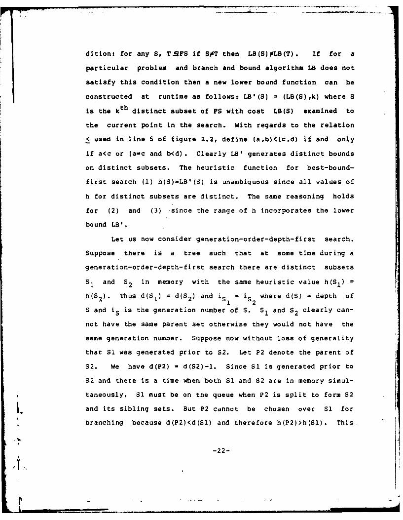
Figure 2.4. A and Ab in case 2 of proposition 2.2. The inferred

state of the priority queue is given under s in A and r in Ab.

The topmost entries have the highest priority.

~b -

h(s)<h(r) i must follow s in A, thus ; follows s in A. But

this means that ; is out of order contradicting our assumption

that s is the first node in Ab out of order. QED

The following lemma asserts that exactly those nodes are

examined in a branch and bound search wih finite initial bound

whose parents have a cost within the current value (at examina-

tion time of the parent) of the bound.

Lemma 2.1: For any node M in A, except the initial node N0 , and

for any finite integer b, M is examined by BB(N0 ,b) if and only

if LB(M')<Bbndex(M,), where M'=parent(M) and index(N) is the

index in A of node N. LB is the lower bound function.

proof: If part: We will show by contradiction that all nodes in

A except N satisfy this half of the lemma. Let 1 be the first

node in A which is not examined by BB(N 0 ,b), and whose parent,

M4', has cost cost(M'KB We can show that M' is exam-M', as cst ost(')<index(M,).

ined by BB(N 0 ,b) as follows: if M'-N 0 then we already know that

M' is examined since the initial node is always examined by BB.

Otherwise let M"parent(M'). We can show that

-25-

I'

LB(M*)<Bbndex(M4,). We have LB(M")<LB(M') by condition 2 of thebb

definition of a lower bound function, and Bindex(M >B b

since M comes before M' in the node ordering of A and the se-

quence Bb is nonincreasing. Thus we have

LB(MO<LB(M')<BbdM , )< BbndexlMu) . Since we have assumed

that M is the first unexamined node in A such that

LB(M')<Bbndex() it must be that M' is examined by BB(N0 ,b).iBB(No(b) •

When M' is examined we have LB(1')<Bndex(M) i.e., the lower

bound of M' is within the current value of the program variable

bound, thus the test of line 5 in Figure 2.2 evaluates to true

and the sons of M' (including M) are inserted in the priority

queue for later examination. For any finite initial bound b,

there are only a finite number of nodes with a lower bound less

than b and since any node can insert a finite number of sons in

the queue, there are only a finite number of nodes inserted in

the queue during the execution of BB(N0 ,b). This means that

after a finite time the node M must be examined. This state-

ment contradicts our assumption that M is not examined by BB,

so our assumption that there is a node that is not examined

under the condition of the lemma must be false.

For the only if part: if M is examined by BB(N 0,b) then

by definition M was inserted in the priority queue at some

time. This could only be if, when the parent of M, M', was ex-

amined, the test of line 5 in Figure 2.2 evaluated to true,

i.e., LB(M')<bound=SB'ndex(M,). QED

I.It can now be shown under what conditions BB will solve

-26-

21

an instance of a combinatorial minimization problem.

**

Theorem 2.1: For finite b>c where c is the cost of a least

cost object in FS, BB(N0 ,b) will find an optimal solution of

cost c in a finite amount of time.

If c* is the cost of a least cost object in FS then for

all nodes in A, Bb>c* where i ranges over the nodes of A ( we

have B b>c , and there is no object in FS which could lower the

bound below c ). Let s be the first node in A which

represents a subset of FS from which the branching rule ex-

tracts a least cost object of cost c . The parent of s clear-

ly has a lower bound<c so by lemma 2.1, s is examined by

BB(N 0 ,b). Thus SB(N0,b) finds an optimal solution. Again

since only a finite number of nodes are involved when b is fin-

ite BB terminates in a finite amount of time. QED

We conclude this chapter with the following theorem which

asserts that it is worthwhile to find as tight an initial bound

as possible on the cost of the optimal solution in order to

minimize the amount of work necessary to find the optimal solu-

tion.

Theorem 2.2: For a particular instance of a combinatorial

minimization problem p-(FS,cost) where costeCOST n in class Cn ,

let ET(h,p,b) be the number of subsets examined by BB(N 0 ,b) us-

ing the search strategy realized by h. For all h and all b,b'

-27-

ruch that b'>b>@, ET(h,p,b).<ET(h,p,b1).Proof: The theorem follows easily from the following lem-

ma.

Lemma 2.2: For all i and b'>b, BbBbe

Proof by induction on i. For 1=0, B b=b and B b'b so the

lemma holds. Next assume B <be fo sm i will be

changed from the value B . 1 olyi B( 0 b examines Ai~ andonlyif B(No~) b

it represents a solution which changes the bound. If B > B.'

it must be because Bb1 = cost(A1 1,) but B1 remains unchanged.

Let A. be the parent of Aj-1* Aj-1 is unexamined in BB(N,,b)

if cost(A.)> B.b by lemma 2.1. But since Aj~ is examined by

BB(N,,b') we have cost(A )(B. , thus B. <B. which contradicts

our inductive assertion. So <Bb

Let A.i be a subset examined by BB(NO1 b) , Let A. denote

b b bthe parent of A1 . By lemma 2.1, cot(KB and Bbbyl

ma 2.2, so cost(A )<Bb'. Thus A. is also examined by BB(NO,b')) I 1

according to lemma 2.1. If every subset examined by BB(NO1 b)

is also examined by BB(NO,b') then ET(h,p,b)<ET(h,p,bl). QED

-28-

L

Chapter 3.

Computational Complexity

and a Model of Branch and Bound Search Trees

3.1 Random Problems and Random Trees

In the previous section it was noted that the branch and

bound process generates a tree structure. In this chapter we

use this abstraction to define a probabilistic class of trees

which models the kind of tree structures that BB generates over

*the instances of a combinatorial minimization problem. Within

this model then it makes sense to derive expressions for the

expected time and space requirments of BB under various search

strategies. The set of subsets of FS that are inserted in the

priority queue during the execution of BB is called the search

tree and the time complexity of a branch and bound search will

be measured by the size of the search tree. The space

complexity will be measured by the maximum number of subsets in

the queue at any time during the search. The time and space

complexities of a given search by BB will sometimes be denoted

by the variables N T and N5 respectively. This definition of

time complexity does not include the amount of time spent exe-

cuting the branching rule or inserting nodes in the queue. A

branching rule is a feature of a particular algorithm and lit-

tle can be said about it on the level of abstraction aimed for

ir -29-

in this dissertation. We assume that these factors are rela-

tively independent of the rest of the branch and bound process

so that the product of the average branching time per subset,

the average time spent inserting a node in the queue, and the

total number of nodes inserted in the queue (the time complexi-

ty) is a reasonable approximation to the running time of a par-

ticular problem on a machine. Again though our goal is to com-

pare the expected performance of various search strategies on a

problem. On a given problem the branching time and node inser-

tion time should factor out of this comparison leaving the size

of the search tree as the essential measure of performance.

The question of interest is how can we model the behavior

of BB on a random instance of a problem apart from the details

of the problem. I.e, what features of a branch and bound

search are relevant to branch and bound and what are problem

dependent? First by the action of the branching rule a tree

structure is generated, so BB is a tree searching algorithm.

Secondly the lower bound function of BB associates a number

with each node in this tree. The search strategy does noc af-

fect the tree per se, but only the order in which the algorithm

examines the tree. So a tree with costs associated with each

node is another way of expressing the domain of BB. In this

setting the goal of Ba is to find the least cost leaf of the

tree. These considerations are formalized in the following de-

finition. An arc-labelled tree is a tree T=(N,A,C) where N is

a set of nodes, A is a set of arcs, and C:A->Z (positive in-

tegers) is a cost function on the arcs of the tree. For exam-

-30-

Figure 3.1. An arc-labelled tree

pie see figure 3.1. In an arc-labelled tree the cost of a node

is defined to be the sum of the costs on the arcs on the path

from the root to the node. The cost of the root is zero.

The next step is to map the notion of a random instance

of given size into the arc-labelled tree domain. A probability

function is assigned to the class of arc-labelled trees which

should somehow correspond with a probability distribution on a

combinatorial minimization problem. Our model of this mapping

is to regard the generation of a tree as a random process in

which each application of the branching rule is replaced by an

independent random experiment where the outcome is the number

of sons that a node has. In a similar manner the assignment of

a cost to a node is tr-ated as the outcome of a different in-

dependent random experiment. Formally let P and Q be probabil-

ity mass functions. It is assumed that P and Q satisfy the

following properties:

1. P(0) > 0 (a node is terminal with nonzero probability)

2. Q(0) = 0 (an arc has cost zero with probability zero).

The algorithm in figure 3.2 generates a random arc-labelled

tree. Let RANDOM(F) be a random function which returns k with

1' -31-

I'

probability F(k). This dynamic means of defining a random

arc-labelled tree is easily implemented for experimental pur-

poses on a machine.

This process is related to the well-known branching pro-

cess (Harris 1963] which has applications to population growth,

nuclear fission reactions, and particle cascades. The basic

branching process is essentially the same as the process in

figure 3.2 except that sprouting may be done in parallel and

there is no arc-labelling. The initial node in a branching

process is viewed as an individual who gives birth to k indivi-

duals with probability P(k), who in turn give birth to new in-

dividuals, and so on. The number of nodes at depth d in the

generated tree is the random variable of interest and it is in-

terpreted as the size of the population at time d. The theory

of branching processes is concerned with the distribution and

moments of the population size as a function of time, the pro-

bability of extinction (i.e., whether the'tree is finite or in-

finite) , and the behavior of the process in the case that the

population does not die out. In contrast our concern here is

with the behavior of the algorithm BB on a randomly generated

tree. In general only a small finite portion of the tree will

be searched by BB.

We will need to define a probability function on the set

of arc-labelled trees. This can be accomplished as follows.

The generation of a tree is viewed as a sequence of trials,

where each execution of step 2 in figure 3.2 is a trial. Let n

-32-

Figure 3.2. Generating a random arc-labelled tree.

1. Let a root node exist. The root is unsprouted.

2. Select an unsprouted node n (according to some search stra-

tegy) and sprout it as follows:

Let n have RANDOM(P) sons. For each arc from n to its

sons label the arc with cost RANDOM(Q).

3. Repeat step 2 until all nodes have been sprouted.

denote the number of sons generated in a random trial and let

Cl,c 2 ,...,cn denote the arc costs assigned to the arcs. The

probability of the outcome of a trial then is

P(n)Q(cl)Q(c 2 )...Q(cn). Clearly if we sum over all possible

outcomes of a trial, the probabilities sum to 1,

03 (3) a)a P(n) I Q(cl )... 5 = 1.

n=0 C=l 1 C n=l

We can formulate the probability of a tree generated by this

process as follows. Consider the probabilities of the outcomes

of the trials during the generation of a tree in a sequence

<g0 0g1 P g2 ... >P where gi is the probability of the particular

outcome of the ith trial. Let us call the product ggl...g i

the ith partial probability of the randomly generated tree.

The probability of a randomly generated tree then is the limit

as i goes to infinity of the ith partial probability. For ex-

ample, the probability of the arc-labelled tree in Figure 3.1

is P(2)*Q(1)*Q(2)*P(O)*P(3)*Q(3)*Q(5)*Q(7)*P(0)*P(O)*P(0). It

is our special assumption that each trial is independent of all

other trials that enables us to take the product of the proba-

ir -33-

r -- '-

bilities of the individual trials as the probability of the

tree. A more formal approach to this probability function over

the set of arc-labelled trees can be based on the measure-

theoretic treatment of trees generated by a branching process

found in [Mode 1971, pg. 3-6].

If the tree generated by our process is infinite then the

limit of the partial probabilities Will Usually go to zero

since we are considering the product of numbers between 0 and

1. Although the probability of generating a particular infin-

ite tree is usually zero, it can be shown that the probability

that a randomly generated tree is infinite is nonzero for many

probability functions P. This fact is a basic result of the

theory of branching processes [Feller 1963, pg. 7] and may be

stated more precisely as follows: Let 7 denote the mean of P.

If F<1 then a randomly generated tree is finite with probabili-

ty 1. If F>1 then a randomly generated tree is infinite with

probability 4, where 4 is the least positive fixed point of the

generating function for P: qp(q) where

00 kp(s) I P(k)sk=0

A randomly generated tree is finite with probability 1-4. By

an infinite tree we mean not only a tree with unbounded depth

but also that the number of nodes at depth d grows unboundedly

in d. It turns out that the probability that a random tree has

unbounded depth but a bounded nonzero number of nodes on all

levels is zero for all P.

-34

Let sons(N) denote the number of sons of the node N. The

arc-labelled tree T is in the class of (PE.q)-trees if and only

if P(sons(N))> for all neN and Q(C(a))>0 for all aeA. E.g.,

if a node in T has 11 sons but P(ll)-O then T is not a

(PQ)-tree.

The remainder of this dissertation is concerned with the

expected performance of BB on the class of (P,Q)-trees for ar-

bitrary P and Q. All theorems about (P,Q)-trees are implicitly

quantified over all probability mass functions P and Q though

it may not be stated. It is important to ask how successful

this transfer is of the notion of random problem instance to a

random (P,Q)-tree. Can we predict (through careful choice of P

and Q) the expected performance of BB on a combinatorial minim-

ization problem by finding the expected performance of BB on

the class of (P,Q)-trees?

The key asumption in this model is the independence of

each application of the branching rule and the independence of

each assignment of arc costs. It might be expected however

that the degree of a node depends somewhat on the depth in the

tree. In particular for finite trees the probability that a

node has zero sons should go to one with increasing depth.

That these observations are so for the traveling salesman prob-

lem is borne out 'by table 2 in chapter 7.

In defense of this model it may be noted that this is

perhaps the simplest possible model of branch and bound trees

and should prove more amenable to analysis than a more complex

-35-

I' ' .. .-

model. With regards to the independence assumption, for suffi-

ciently large trees the branch and bound process examines only

the topmost part of the full tree which may have much more uni-

form properties than the tree as a whole. We present evidence

in chapter 7 that the theory of (P,Q)-trees can be applied with

good predictive power to a branch and bound algorithm for solv-

ing traveling salesman problems, and we conjecture that the

model is applicable to at least those branch and bound algo-

rithms which employ a relaxation procedure.

Some notation follows which will be needed. For a random

variable x and a probability mass function p(x), the expected

value and variance of x are computed by

E(x) = 5 x p(x)x

a2 = E(x2 ) - E(x) 2 .

The first and second r,,oments of P will be denoted P and

respectively, i.e.,

- kP(k) andk>0

= 2 P(k,.k>0

3.2 Properties of a Class of (P,Q)-trees.

Before studying the behavior of BB on (P,Q)-trees it will

be useful to develop expressions for some important properties

of a class of (P,Q)-trees. For example what is the expected

-36-

/ '

I' li II . .. II

path length of a randomly picked path in a randomly picked

tree? The probability that a node is a leaf is P(O) and the

probability that a node has some sons is l-P(0). A branch of

length k then has probability ( 1 -P( 0 ))kP(O), a geometric dis-

tribution. The expected path length is

3 k(l-P(s))kP(O) - (l-P(0))/P(0). (1)

k-0

A more difficult question concerns the distribution of least

cost leaves over the class of (PQ)-tregs. Let opt(T) denote

the cost of the least cost leaf in an arc-labelled tree T. Let

O(i) denote the probability that opt(T)=i in a random

(P,Q)-tree T. 0 is defined on the nonnegative integers since

the cost of any leaf in a (P,Q)-tree is a nonnegative integer

by definition. A recurrence relation for 0 can be formulated

by equating two expressions for the probability that opt(T)>i

in a random (P,Q)-tree T. First note that no arcs can have a

cost of zero so the only way that a tree can have a least cost

leaf of cost zero is if the root is terminal, thus 0(0) = P(0).

One expression for the probability that opt(T)>i is

I 0(k). (2)

k=0

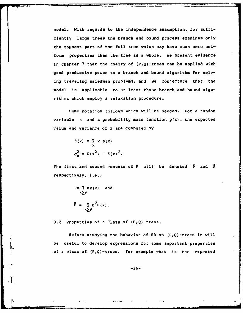
Next consider the treetop shown in Figure 3.3a. The subtrees

TT2,...,Tj are themselves random (P,Q)-trees. The probabili-

ty that opt(T'k)>i where V'k is the kth subtree plus the arc

from the root as in figure 3.3b is*i S

i - 3 S Q(c)O(s-c). (3)S-1 c=l

.7

, -37-Af

r

Figure 3.3a. A Tree-top. 3.3b. A Branch

This expression sums over all combinations of arc costs c and

costs of least cost leaves within T (letting s denote the least

cost leaf of the combined arc and subtree, s-c is the cost of

the least cost leaf of the subtree) for which the sum is not

greater than i. Since this expression applies independently to

each of any number of branches, the probability that the tree-

top of Figure 3.3a has j branches and opt(T)>i is

i sP(j)[ - 5 5 Q(c)O(s-c)] j .

s=1 c=l

For i>0 the probability that opt(T)>i in a random (P,Q)-tree is

O i sP(j) [I- 5 Q(c)O(s-c)] . (4)

j=1 s=1 c=l

The case j=0 is not included in this expression because then

opt(T) = 0. Finally expressions (2) and (4) can be equated:

i O i s1 - I O(k) I P(j)[l- I I Q(c)O(s-c)] j . (5)

k-0 jl sinl c-l

This is a recurrence relation since 0(i) appears on the left

but only the values 0(0), 6(1), ..., 0(i-1) appear on the right

-38-

I' I I

for i>l. In the appendix this recurrence relation is broken

down into simpler recurrence relations in order to speed up the

computation of 0. Except for special P and Q this recurrence

relation seems to have no general analytic solution. Empirical

data on uniformly distributed P and Q suggests that 6(n) is

asymptotic to dn as n-)c for some constant d that depends on P

and Q. Figure 3.4 shows some of 0 for the class of

(P1 ,Q1,)-trees where P1 0 (k) - i/Il if and only if <k<10, and

Q1 00 (c) = 1/100 if and only if 1<c<100.

Figure 3.4. O(i) for (Pl0,Q1 0 0 )-trees.

A.1. 0(e

.0 1. ....................................................

.OOG * ... -""* .... .. ..o- I*

"4 ia a",to 1, '

Let dep(T) denote the least depth at which a least cost

leaf may be found in an arc-labelled tree T. A generalization

of the function 0(i) is the function d(i,k) = probability that

opt(T)=i and dep(T)-k in a random (P,Q)-tree T. In a manner

similar to the derivation of (13) above, a recurrence relation

I. .can be formulated for d(i,k) by equating two expressions for

the probability that opt(T)>i or (opt(T)=i and dep(T)>_k).

-39-

i-i j k1 - 2I d(j,m) - I d(i,m)

j=O m=O m=O

Co i 1-2 i-c-1 m2 2 P(j)[1- 2 Q(c)d(O,O) - 2 Q(c) 2 2 d(m,n)

j=l c=1 c=1 m=1 n=1

i-1 k-1- I Q(c) I d(i-c,m)]j (6)

C=1 mZ1

where d(0,0) = P(O)

d(i,m) = 0 for m>i

d(i,O) = 0 for i>O

Note that the left hand side of (6) nas the term d(i,m)

whereas the righthand side uses only the terms d(j,k) for j<i

or (j=i and K<m).

By taking marginal sums of d(i,m) we obtain two important

functions concerning the class of (P,Q)-trees. First we can

derive the recurrence relation (4) for 6(i) again since:

O(i) = E d(i,m) = d(i,m) for i>0 (7)

1=0 m=1

Secondly, let DEP(m) be the probability that dep(T)=m in a ran-

domly generated (P,Q)-tree T. This function is given by

oDEP(m) Z 2 d(i,m) (8)

i=M

Figure 3.5 shows an example distribution of DEP(m). Note that

DEP(m) quickly approaches zero as m increases.

I.

t -40-

Figure 3.5. DEP~m) for the class Of (P10,Q100)-trOCS.

.36L 3

4D2

* 1

Chapter 4.

Heuristic Search Strategies.

Subsequent chapters will investigate some particular well

known search strategies but it seems appropriate to first look

at search strategies in general. In chapter 2 the function

ET(h,p,b) was defined as the time complexity for solving the

problem instance p when BB uses the search strategy realized by

the heuristic function h and is given an initial bound of b.

Define the expected time complexity of a heuristic search of a

random (P,Q)-tree as

ETh(b) = S Pr(t)ET(h,t,b) (1)

t

where t varies over all (P,Q)-trees and Pr(t) is the probabili-

ty of t as defined in the previous chapter. Of particular in-

terest for comparison purposes in this thesis will be the limit

as b goes to o of ETh(b), denoted by E(NT) or ETh(O).

The time complexity of a branch and bound search may be

viewed as a random sum of independent variables. The ith such

variable is the number of sons inserted on the queue by the ith

0explored node. Let Gh(k) denote the probability that exactly k

I. nodes are explored during the search of a random (P,Q)-tree

under search strategy h. If we let Xi denote the number of

Asons that the ith explored node has then the size of the search

-42-

tree, denoted by the random variable NT, is a random sum 1 + X1

+ x2 + ... + Xk where each Xi is distributed according to P and

k is distributed according to Gh. See section 3.1 for the de-

finitions of ' and P.

Theorem 4.1. Let NT = 1 + X1 + X2 + ... + Xk be a random sum

where each variable Xi is distributed according to P and k is a

random variable distributed according to Gh, then

E(NT) - 1 + Gh (2)

2 r_ F h -2NT + ( h Gh). (3)

Proof: Let p(z) and g(z) be the generating functions for

P and Gh respectively, i.e.

g(z) I G h(n)z, p(z) = P(n)zn=0 n-

It is a well-known result (c.f. Feller 1959 pg. 286-287) that

the generating function for the random sum X1 + x 2 + ... + Xk

is g(p(z)). It can also be shown (Feller 1959, pg. 265-266)

that for a variable x distributed according to F(x) with gen-

erating function f(z),

f(l) - 1 (4)

E(x) f' (1) (first derivative of f) , (5)

Let f" denote the second derivative of f, then

fW(1) = P - V (6)

(, '2 = f"(1) + f. (1) - f (1) 2 . (7)x

From these relations it is straightforward to derive the rela-

/'! -43-

tions of the theorem. In what follows we use the symbol Dz in

the usual way as the derivative with respect to z.

E(NT-1) - Dz g(p(z))Iz-1 by (5),

- g(p(z))P'(Z)I z 1

Sg' (p(1))p' (1)

s g'(1)p' (1)

Thus we have shown

E(NT) = 1 + p.

The variance can also be derived straightforwardly.2Dz g(P(Z))Iz= 1 M Dz g(P(z))P'(Z)Iz=

=g"(p(z))p'(z)p'(z) + p"(z)g (p(z))Iz=1

= g"M()p' (l)2 + p"(1) ' (1)

= (C - ).2 + ( C- , by (6)

Thus

a = D2g(p(z))Iz= 1 + Dzg(p(z))Iz=l - (Dzg(p(z))Iz,,)N T-1 z z-l+Dgpz)

by (7)

= (GV2 _ U2 + p,) + p _2a-2.

= 2 (a _ +

Now since a2 c2 we haveI.NTl NT, eh

1 F =2( T_2) + . QEDNT

-44-

/ 'l "

We immediately obtain the following corollary.

Corollary 4.1: E(NT) exists if and only if F and exist.

exists if and only if P, , , and d exist.

Since the function P is assumed given, the main task in

the analysis of a heuristic search strategy is to find a formu-

lation for Gh (k). Lower bounds can be found on the means of NT

and NS for any h.

Theorem 4.2. For all exact heuristic functions h,

Eh(NT) > I + F/P(0),

Eh(NS) > 1 + (P-l)/P(0).

Proof: By lemma 2.1 any exact search strategy must ex-

plore the least cost leaf s and all the nonleaf nodes n such

that LB(n)<c(s ). Let h be a heuristic function for a search

strategy which explores those nodes and no others. If we ima-

gine the nodes of a tree laid out in a sequence in order of in-

creasing cost then h explores just those nodes up to the first

leaf in the sequence. The probability that h explores k non-

leaf nodes is given by

Gh(k) = (1-p(0))kP(0) (8)

i.e, the first k nodes in the sorted sequence are nonterminal

(each with probability 1-P(0)) and exactly one leaf s is ex-

plored (with probability P(0)). We have

= K (-P(0))kP(0) = (1-P(0):/P(0) (9)h M

. -45-

'1:.

Also each nonleaf has j sons with probability P'(j) -

P(j)/l-P(0) for j>l, thus

CDP' = jp(j)/(l-P(O)) = F/(l-P(0)) (10)

j-1

By theorem 4.1,

E-(NT) - 1 + (l-P(0))/P(0) * P/(l-P(0))

= 1 + F/P(0).

It follows that for any exact heuristic function h,

Eh(NT) > 1 + P/P(0).

The space complexity of a random (P,Q)-tree under any

search strategy is bounded below by the number of nodes on the

queue when the first leaf is found by the search. Again NS is

a random sum, but a random sum of random variables which are

slightly different from the random variables Xi in NT. Let

G'h(k) be the probability that k nonleaves are explored before

the first leaf is found. G'h(k) is the same as G;(k) formulat-

ed above, so

Z! h = (-P(0))/P(0).

During the exploration of the ith node, the node itself is re-

moved from the queue and Xi nodes are added, thus the net in-

crease to the queue size is Xi-l, denoted X'i. The random

variables X1 are distributed according to P' where P'(x) =

0P(x+l)/(l-P(0)). We have

P' = 5 jP'(j+l) = jp(j)/(1-P())!j=0 j=0

-46-

... ... .

I (j+l)P(j+l) - I P(j+l)

P- (l-P(O))1-P (9)

Therefore

E(N S ) > h ' (mean of the random sum X1 + X'2 + + X'k)IF- (1- 20 ]1...0

SP-(I-P(O)) 1-P(O)

1 + (F-1)/P(0). QED

4.2 Techniques for analyzing a heuristic search strategy.

The state of a branch and bound search process at the be-

ginning of statement 3 of BB (see figure 2.2) can be described

by the state of the priority queue and the value of the bound.

An actual branch and bound process may be described by a se-

quence of such states. If we can give the probability that a

random process in state Si will be in state S. at the next exe-

cution of statement 3 of BB given only that the current state

is Si, then the set of all such states (including an initial

state) and the probabilities of the transitions between states

defines a markov chain. Formally let (S0 S, S, ...} U {F0 ,

F1 , ...} denote the possible states of a search where S0 =

<b0;N0 > is the initial state, and S i = <b;nl,n 21 ...,nk> where b

is a value of the bound and the nodes nln 2,...,nk are on the

queue in that order, i.e., h(nl)<h(n 2 )< ...<h(nk). The final

states are denoted by Fb - <b;> where b is the value of the

bound and the priority queue is empty (an empty priority queue

-47-

terminates BB). Let rij denote the probability that the pro-

cess in state i will make a transition from state i to state j.

Let R denote the (infinite) transition probability matrix

Erij]. Suppose we wish to describe the behavior of BB under

search strategy h and given an initial bound of b,. The initial

state is <bo;N 0 >. The transition probabilities may be

described as follows.

The transitions

<b;nl,n2,...,nk>-> <b;n 2,...,nk> (1)

occur with probability 1 for all states in which b<c(n I ).

These transitions reflect the act of pruning the subtree below

n1 as effectively happens when statement 5 in figure 2.2 is

false. The transitions

<b;nl,n2,...,nk> -> <c(n l );n2 ,...,nk> (12)

occur with probability P(0) for all states in which b>c(n I ).

These transitions reflect the action taken by BB on states for

which statement 5 is true and statement 7 is true. (a leaf is

found which improves the value of the bound). The transitions

<b;nl,n2, ... ,n> -> <b;ml m2 ,...,mk l+> (13)

occur with probability P(j)Q(c 1 )Q(c2 )...Q(cj) where

[mlm 2 ,...,mkl+j } = {nln 2 ,...,nknl+clnl+c2,...,nl+ c }

and h(m,)<h(m2)<...h(mk-l+j).

These transitions reflect the action taken by BB on states for

-48-,I

which statement 5 in figure 2.2 is true but statement 7 is

false; (the sons of a node are added to the queue for later ex-

ploration).

Since a node is removed from the queue at each transition

the number of transitions from the start state to a final

state, called the first passage time for a random process, is

the number of nodes inserted on the queue during the search;

i.e., the time complexity. There are well-known methods for

finding first passage times and their means (Parzen 1973], but

they are not of much help when the transition matrix is infin-

ite. A sequence of states [S OSl ...,Sd is realizable if S0

is the initial state, S n is a final state, and for 0<i~n

r sii~ >0. The set of all realizable sequences defines the

sample space on which our random variables N T for the time com-

plexity, and Ns for the space complexity are defined. The pro-

bability of a realizable sequence is defined to be

n-lH r5i=0 sii+l*

Insight is needed into the nature of a particular search

strategy in order to coarsen this sample space into appropriate

events such that an expression for the expected complexities

can be derived. Theorem 4.1 offers some help in this direction

by defining the event En as the set of all realizable sequences

in which exactly n transitions of the types (12) and (13) ap-

pear. We have defined the probability of event E as G()n Ghn)

Since P is given and it is assumed that F can be found, the

-49-

problem of finding E(N T reduces to finding a reasonable ex-

pression for ff.h perhaps by first finding G h(n).

Complementing this general approach to finding E(NT) and

E(N s for a heuristic search strategy# there is a more ad-hoc

method. In this approach we observe how the data structure

which is normally used to implement the search strategy is af-

fected by searching a random (P,Q)-tree. Special properties of

these data structures may help in the analysis. For example, a

depth-first search is usually implemented using a stack. The

close relationship between stacks and the implementation of re-

cursion suggests that a recurrence relation may be the best way

to describe an algorithm employing a stack.

-50-

Chapter 5.

The Best-Bound-First Search Strategy

The best-bound-first search strategy as realized by 3-(l)

chooses to explore the least cost unexplored node on the prior-

ity queue. The following theorem gives a characteristic pro-

perty of this search strategy.

Theorem 5.1. The first leaf explored in an arc-labelled tree

by BB under the best-bound-first search strategy is optimal.

Proof: Best-bound-first explores the nodes of a tree in

order of increasing cost. The first leaf s which is explored

then is optimal since all nodes (including leaves) which could

be explored subsequently have at least as great a cost as s*.

QED

As a result of theorem 5.1 it is not neccesary to explore

all stored nodes in a best-bound-first search. By the nature

of the heuristic function all nodes on the queue when the first

leaf has been found have a cost greater than or equal to the

cost of the leaf. Therefore there is no need to explore any

further nodes and the search may terminate. More generally,

whenever a search strategy has a best-bound-first component

(e.g. in ordered-depth-first, ordered-breadth-first) as soon as

-51-

a leaf is found or a node with greater cost than the bound,

then no more nodes need be examined from the priority queue.

Theorem 5.2. The expected time and space complexities of a

best- bound-first search of a random (P,Q)-tree are,

Ebbf (NT) - I + P/P(O) (1)

£bbf(NS) i + (F-1)/P(0) (2)

Proof: Since the best-bound-first search strategy exam-

ines nodes in order of increasing cost, it is a special case of

the heuristic function h analyzed in theorem 4.2. Therefore

the results derived for h also hold for best-bound-first

search. QED

As a consequence of theorem 5.2 the best-bound-first

search strategy is optimal both in terms of time and space

within our model. Using theorems 4.1 and 4.2 it is possible to

derive expressions for the variances of NT and Ns also.

Theorem 5.3. The variances of the performance of a best-bound-

first search on a random (P,Q)-tree are

.2 M PF2 /P(0)2 + P/P(0) (3)N7iT

(72= F-l) 2 /P(0)2 + (p-l)/P(0) (4)NS

Proof: The random variable NT is a random sum 1 + X1 + X2

-52-'I

+ where Xill has the probability

P'(Xi) - P(Xi)/(l-P(0)),

and the probability that there are k terms (the number of non-

terminal nodes) in the sum is

G(k) - P(O)(1-P(O))

as in theorem 4.2. The variance of NT is

(Y.2T =,2_.2)+ ,.(5)

by theorem 4.1. We have

= , P(X)

X1 l-P( e ) i-p(S)'

= x2 P(x)

X=l l-P() -P(0)'

I kP(O)( 1-P(O))k = P(0)

k=0 P()

We can find an expression for a - , which is needed in order

to evaluate (5), as follows.

-1 (k -k)P(0) (l-P(5)) = k(k-l)P(0) (l-P(0))k-0 k=0

LetCD k k P(O)

GG(z) = I P(0)(1-P(0)) z = 1____ ___k=0 l-z (l-P (0)) '

by taking the second derivative of GG with respect to z, we

get,

CD k k-2GGO(z) 2 k(k-l)P(0)(l-P(0)) z. .k= 0

k-O-D2 P(O)(l1-z(l-P(0))] -

IL

' _,-53-

i, I . . .- ik : i ..

= F(SPi) (l-F(el))[l-z(1-F,(S))] -

2P() (1- P())2

[1-z (1-P (0) ) ] 3'

Then - GG(l)

2P(0) (-P())2

(1- (1-F 0)) ]

-2 (1-F(S0) )2

P(O)

Substituting all these terms into (5), we obtain,

rN T (1-p())2 P(0) 2 P(02 ') + TO

F(S)2 P--1"F2 2

The expression (4) for 2 can be derived in a similar manner.

QED

For example consider the class of (Pr,Qs)-trees where

Pr (k) = i/r+l for O<k<r, and Qs(c) = 1/s for l<c<s.

E(NT) - 1 + (r/2 -1)/(l/r+l) ) = O(r 2 ),

a-. -= ((r/2)/(l/r+l) _1) 2 + (r(2r+l)/6 -1)/(l/r+l)NT

= 0(r 4 ).

If (Pr' Qs ) were a good model of the trees generated by a par-

ticular branch and bound algorithm under a best-bound-first

search strategy then the algorithm would have an expected

2. -54-

21

search tree size of O(r ) and a variance of O(r 4). Note that

the space complexity of best-bound search is the same order of

magnitude as its time complexity.

Some comments are in order here. First, the time and

space complexity of a best-bound-first search do not depend on

Q, the distribution of arc costs. Only the relative ordering

of nodes in a tree is important to a best-bound-first search,

not the particular costs. This fact together with the assump-

tion of mutual independence of the nodes of a (P,Q)-tree ac-

count for the absence of Q in (1) and (2).

Second, although the assumption of our model doesn't gen-

erally hold for interesting combinatorial minimization prob-

lems, (1) can be used to obtain an upper bound on the expected

time complexity of a problem. Simply stated, the product of an

upper bound on F (average degree of a random node) and an upper

bound on 1/P(0) (P(0) is the probability that a random node

supplies a feasible solution) yields an upper bound on the ex-

pected time complexity. In chapter 7, we derive bounds along

these lines for a subtour-elimination algorithm for the travel-

ing salesman problem. Following the discussion above, upper

bounds on F and 1/P(0), namely O(ln(n)) (order of the natural

logarithm of n) and n/e respectively, are multiplied to obtain

an estimated upper bound ( nln(n)/e) on the expected time com-

plexity.

-55-(:,

Chapter 6.

Depth-First Search Strategies

6.1 Expected Time Complexity

The choice of which node to explore next in a depth-first

search is made between the sons of the most recently explored

node (if any), otherwise the sons of the next most recently ex-

plored node, and so on. In an ordered-depth-first search (odf)

the sons are explored in the order of increasing cost as real-

ized by the heuristic function in equation 2-(2a). If the sons

are explored in the order of generation, then the search is

called a generation-order-depth-first search (godf) as realized

by the heuristic function in equation 2-(2b). Let ETodf(b)

denote the expected size of the search tree generated by BB on

a random (P,Q)-tree using the ordered-depth-first search stra-

tegy and given an initial bound of b. Let ETgodf (b) denote the

corresponding expected value for a generation-order-depth-first

search. Expressions for these functions can be formulated

fairly naturally as recurrence relations. Suppose that BB is

searching a tree with the structure shown in Figure 6.1 where

each subtree TIT 2 , .... T may be regarded as a random

(P,Q)-tree. Let b1 be a finite initial bound (the bound on the

root) and let bi denote the bound at the top of the subtree Ti

for l<i<j. Then the expected size of the search tree for a

-56-

'E

random tree with this structure is

1 + ET(bl) + ET(b 2 ) + . . . + ET(bj).

Each of the bounds bi for 1<i<j is less than b1 indicating that

a a recurrence relation may be set up. The next problem con-

cerns the probability of a given bound occuring at a given

node. Consider the tree in Figure 6.1. Given an initial bound

of b., the bound on the subtree T1 is bo-c 1 so BB is expected

to search ET(b -c,) nodes in T1 . opt(T I ) = m with probability

O(m) since it is a random (P,Q)-tree. The same holds for the

other subtrees. Suppose that opt(T 1) = Vl. If ml>=b I then the

search will not find the least cost leaf. On the other hand if

Ml<bI then the search will find the it. To summarize, the

bound returned after searching the first subtree of the tree of

Figure 6.1 with initial bound b is minib 0 , cl+m }. The bound

on the subtree T2 is mintb0 , cl+ml}-c 2. Continuing this rea-

soning one finds that the bound on the ith subtree Ti is

bi = min{b 0 , cl+M 1 , c2 +m2, ... I ci_ 1 +mi_ 1 } - ci (i)

where m lm 2 ,...,mi_1 denote the least cost leaves of the sub-

trees T1 ,T2 ,...,Ti_1 respectively. ET evaluated with expres-

sion (1) yields the expected size of the subtree Ti .

The following function gives the expected size of Ti over

all (P,Q)-trees. Let the functions Wdodf(b,i) and Wdgodf(bi)

denote the expected size of the search tree of Ti when the root

is given an initial bound of b for an ordered-depth-first

-57-I

Figure 6.1 A tree-top.

search and a generation-order-depth-first search respectively.

An expression for Wdgodf(b1i) can be found by essentially

enumerating over all possible combinations of variables in (1).

Wd godf (b~i) -

1 .. c 1 m 5=0 .. m Q1)..1=0Omlo.~m_)

ETgodf (in~b,c 1 +m 1 1... ,ci- 1 +M i 1}-ci) (2)

A tree with a structure as in Figure 6.1 will have expected

size

1 + Wd (b,i).1= godf

This expression summed over all j (number of sons of the root)

gives an expression for ETgod(b):

ETgod(b) 3 PUj)(4- 1 Wd(b,i))j=0 in i=l

=1 + P(j)ilWgd (b,i). (3)

As stated, (2) is computationally intractable; however it can

-58-

refined to a more computable form as given in appendix A.

The order of examining the subtrees of figure 6.1 by an

ordered-depth-first search is treated as follows. In an arbi-

trary (PQ)-tree with this structure, the arc costs

C lIC21...PC are unordered. By rearranging the tree the arc

costs can be brought into sorted order. Note though that a

given ordered sequence c 1 <c2 _<...<c i may result from the sorting

of many distinct sequences. The appropriate combinatorial

question is how many unique arrangements Ri(clC 2i...,c i) of

this sequence there are. There are il nonunique arrangements

but repetitions must be accounted for. If k of the i values

have the same value cj=cj+l=.. .=cj+k then there is a repetition

factor of k1 due to this relation. In general

Ri (clc 2 ,...,c i ) = i!/rllr 2!...rk!

where

C=... =C <Cr + cr

1 2 k-i rl+r2+...+rk

and r1+r2 +...+rk=i. (i.e., there are r1 variables with the

same value, r2 variables with the same value, and so on)

Again by enumerating over all possible ordered sequences

Cl,...,C i and ml,...,mi_ 1 of the variables in (1), an expres-

sion for Wdodf(b,i) can be found.

,. Wdodf(bi) =

5 5 ... Q(cl)Q(c 2 ) ...Q(ci)* Ri(cl'c 21'...'ci)

c=l c2=cl i-1=ci

-59-

t ,1.. .

=0 .. =0O( 1 1 ...O(mii)'mI = miI -0

*ETodf (minb,c 1 + MI ,c2+m 2 , ... ,i_ 1 + m i -1-c )(4)

A tree with a structure as in Figure 6.1 will have expected

size

1 + Wdodf(b,i).

i--I

This expression summed over all j (number of sons of the root)

gives an expression for ETodf (b):

jaETodf(b) = 2 P(j)(I+ 2 Wdodf(b,i))

j=O i=1

0 j= 1 + I P(j) I Wdodf(b,i). (5)

j=1 i=1

Hereafter we will omit the subscript on ET and Wd except

when necessary since all properties to be given have the same

form for both. (i.e. the following theorems will hold with ei-

ther subscript added). When the limit of the sequence ET(b)

exists, it will be denoted ET(co). Clearly when this limit ex-

ists we have the existence for each i of the limit of Wd(b,i),

denoted Wd(cc,i). In corollary 4.1 we found necessary condi-

tions for the existence of ET(co), i.e. the existence of l and

G . Henceforth we will restrict our discussion to classes of

(P,Q)-trees for which ET(co) exists. We suspect that those

I. classes of (P,Q)-trees for which the limit of ET does not exist

are not particularly interesting in that they cannot be good

models of combinatorial minimization problems.

-60-

Several results about these limits can be shown. Theorem

6.1 asserts that the expected size of a search tree is the same

as the expected size of the search tree of the first subtree of

the root.

Theorem 6.1. ET (a) Wd(o,l1) .

Proof: limit Wd(b,l) - limit I Q(c)ET(b-c) by (2),b-)m b-)co c-i

I Q(c)limit ET(b-c)

=ET (o) 5 Q(c)c-1

ET (c) . QED

Theorem 6.2 gives an expression for ET(o) which is similar to

that for a best-bound-first search given by eq. 5-1. The quan-

ti1ty W is the expected number of nodes in the search tree ex-

cept those in the first subtree.

Theorem 6.2. ET(d) - W/P (0) where W I + I P(j) Wd(o, i) .j=2 i-2

Proof: ET(co)-l+ S P(j) I Wd (00,j-1 i-i

- 1 + Wd (o, 1) 1 P (j) + I i Wd(OD, ijul j-n2 1-2

- I + ET(03)(i-P(0)) + I P(j) I Wd (o, i)j=2 i-2

by theorem 6.1 thus,

-61-

00 JET(co)=[I+ I P(j) I Wd(o,i)]/P(O) - W/P(O). QED

j-2 i-2

We can reason from theorem 6.2 to a lower bound on ET(w)

which was established by different means in theorem 4.2.

Proposition 6.2. ET(q) > 1 + P/P(0).

Proof: W - 1 + I P(j) Wd(lD,i)j=2 i-2

> 1 + 3 P(j) 1j-2 i=2

= 1 + I (j-l)P(j)j=2

= 1 + 2 jP(j) - 2 P(j)j=2 j=2

= 1 + F-P(1) - (1-P(0)-P(1))

= F + P(0).

Thus ET(Co) = W/P(0) > (P(0)+F)/P(0) = 1 + F/P(0). QED

6.2 Time complexity as a function of the depth of the first

leaf found in a depth first search tree.

The depth at which the first leaf is found in a depth-

first search has a strong effect on the performance of the

search. Intuitively if this depth is deep then the procedure

will spend much of its time examining nodes in that part of the

I. tree before returning to shallower levels where the true least

cost leaf may lie. It might be conjectured that the size of a

-62-

/I .- -

search tree tends to grow exponentially in the depth of the

first leaf which it finds. To the contrary, in what follows it

is shown that a depth first search tree has a structure which

is essentially linear in the depth of the first found solution.

Let X(h) be the expected number of nodes in the search tree ex-

cept those in the first subtree given that the first solution

is found at depth h. X(0) is defined to be 1. See figure 6.2.

Let S(h) be the expected number of nodes searched in a random

3,Q)-tree given that the first solution occurs at depth h.

From these definitions one finds

S(h) = I + h + X(l) + X(2) + ... + X(h)

h= I + h + I X(k)) (6)

k-l

In order to formulate an expression for X(d) an appropri-

ate variant of 0 will be needed. Let 0(d,i) denote the proba-

bility that opt(T)=i in a random (P,Q)-tree T given that the

leftmost branch of T has length d. Similar reasoning to that

which led to the expression 3-(4) for O(i) yields an expression

for O(d,i). Again the method is to equate two expressions for

the probability that opt(T)>i. One expression is

i^1 - 1 O(d,k). (7)

k-n0

Suppose now that the root has j>l sons with subtrees

T,T2,..,T j . This event occurs with probability P(j)/l-P(0)

for d>0 because the condition that the tree has a leftmost

branch of length d disallows the possibility that the root has

-63-

I' --.-

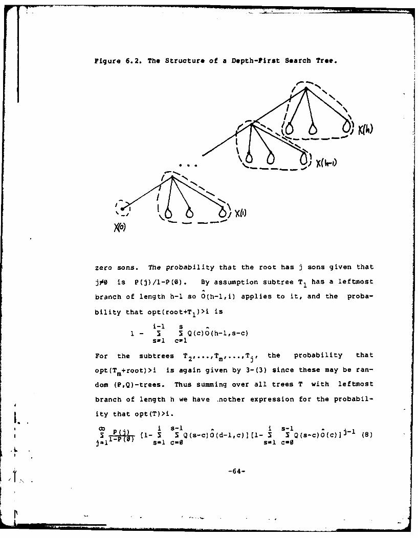
Figure 6.2. The Structure of a Depth-First Search Tree.

"I

X(0)

zero sons. The probability that the root has j sons given that

jog0 is P(j)/l-P(0). By assumption subtree T1 has a leftmost

branch of length h-i so O(h-i,i) applies to it, and the proba-

bility that opt(root+T1)pi is

i-i S1 - 3 3 Q(c)O(h-l,s-c)

s1l c-i

For the subtrees T 2 0' .*IT m ,..T, the probability that

opt(T m+root)>i is again given by 3-(3) since these may be ran-

dom (PQ)-trees. Thus summing over all trees T with leftmost

branch of length h we have nother expression for the probabi.l-

I. ity that opt(T)>i.

CP(i si1 a S. 13 P.T ( C- 5 5 Q(s-c)O(d-l,c)] (1- 5 1 Q(S-c)O(cflj- 1 (8)

j!l sinl c=0 Sui Cin0

-64-

Expressions (7) and (8) may now be equated to establish a re-

currence relation for O(d,i).

I - 5 O(d,k) -

k-0

! s-I c- s-1 c-I

where 0(0,9) = 1 , 0(0,i) - 0 for >0.

The limit of this sequence of probability functions is

expressed as follows.

1 - 3 0(o,k) -k-0

i s-i i s-1'~ P() [1- 5 Q (s-c)O(O,c)] [1- Q . Q(s-c)O(c)] (10)

j=l=1 c=O s=l c

Let LTd denote the subset of (P,Q)-trees whose leftmost

branchs have length d. Let RT denote the set of subtrees of

nontrivial (P,Q)-trees formed by deleting the leftmost subtree

of the root. An arbitrary TeLTd can be realized as the graft-

ing of a tree from LTdl (with attached arc) to a subtree from

RT as in figure 6.3. An expression for X(d) can be found by

summing over all combinations of this form. Let Yd(m) be the

probability that a tree consisting of an arc plus a random tree

from LTd has a least cost leaf of cost m.

m-l1-

Yd(m) I : O(d,m)Q(m-k) (11)k-1

Let Z(m) be the expected size of the search tree of a random

tree T in RT given an initial bound of m. Then X(d) has the

-65-

r I,

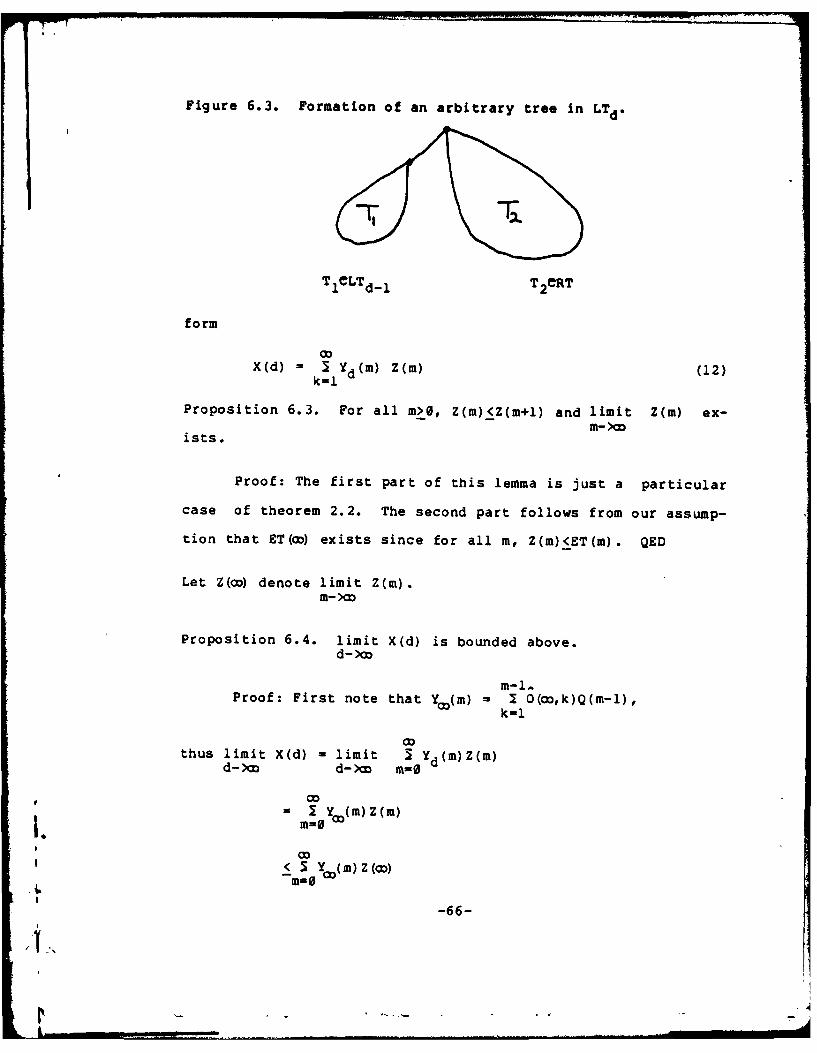
Figure 6.3. Formation of an arbitrary tree in LTd.

Tl1CLTd-1 T 2eRT

form

X(d) - 3 Y d(m) Z(m) (12)k-I

Proposition 6.3. For all m>0, Z(m)<Z(mil) and limit Z(m) ex-m- >CO

ists.

Proof: The first part of this lemma is just a particular

case of theorem 2.2. The second part follows from our assump-

tion that ET(c) exists since for all m, Z(m)<ET(m). QED

Let Z(o) denote limit Z(m) .M- >00

Proposition 6.4. limit X(d) is bounded above.d- )cD

Proof: First note that Y (M) = I O(co,k)Q(m-1),

thus limit X(d) - limit Y Yd(M)Z(m)d-)m d- XD m-0

3 S Y (m) Z(C)

-66-

NI

Z Z(C) IYco(m)-Z (). QEDMOu

Let X(ob) denote limit X(d). These propositions support one ofd- )o

our main results which states that S(d) grows essentially

linearly in d.

Theorem 6.3. S(d) is bounded above and below by a linear func-

tion of d.

Proof: Since X(k)>l, we have

dS(d) - 1 + I X(k) by (6)

k-l

d>1 + 1 - 1 +d.

k-l

Also,d

S(d) = 1 + I X(k) by (6)k-i

d< 1 + I Z(c) by proposition 6.4

k-i

= 1 + Z(Op)d.

Therefore, for all d, we have

l+d < S(d) < l+Z(co) d. QED

Theorem 6.3 can be interpreted as follows: The depth

first search tree can be decomposed along the path from the

root to the first found solution into groups of subtrees whose

expected size is asymptotically constant (the i t h group con-ssso e2 nd 3rd ... r th

sists of the 2nd 3 subtrees below the i node on the

Lpath from the root to the first found solution). See Figure

-67-

I' -

6.2. Therefore the performance of branch and bound is expected

to degrade linearly with the depth of the first found solution.

6.3. Expected Space Complexity of a Depth-First Search

Let ES(b) denote the expected space complexity of a ran-

dom (P,Q)-tree when BB is given an initial bound of b. A re-

currence relation for ES can be set up roughly analogous to the

recurrence relation for ET. First we note that the space com-

plexity must be at least 1 since initially the root is stored

in memory. In terms of figure 6.1, suppose that the root has j

sons. At this point in the search the root node has already

been stored and removed from the queue so we have j nodes in

memory. Let D(b,i) be the expected space complexity of the i th

subtree of the root when the initial value of the bound is b.

When the root has j sons, the expected maximum amount of

storage needed during the search of the ith son is D(b,i) + j-

i. The term j-i accounts for the number of nodes at depth 1

remaining in memory during the search of the ith subtree. The

maximum amount of memory used when the root has j sons is the

maximum over D(b,i) + j-i for all i<j:

max{l, D(b,l)+j-l, D(b,2)+j-2, ..., D(b,j)}.

This expression only has the value 1 when the root has zero

sons since D(b,l)>l (when a subtree is searched, at least the

root of the subtree was once in memory), thus we find,

I. ES(b) = P(j)*max(l,D(b,l)+j-l,D(b,2)+j-2,...,D(b,j))

j-68

e -68-

I/1 '

= P(0)*l + I P(j)max(D(b,i)+j-i} (13)j-1 i<j

where D(b,i) is the expected space complexity of the ith sub-

tree of the root given that the initial bound is b and can be

formulated in the same way that we set up Wd(b,i):

D(b,i) -

C 1.. 1 0... m = olcl1 .Q(C i )Oml) ..olmj 11"*Cl-1~ cj1m J-

ES(min{b,cl+m 1,...,cj_+mj_,1 }-cj) (14)

This expression can be considerably simplified by noting that

for the same reason that ET(b) is monotonically increasing in b

(see theorem 2.2), so also is ES(b).

Proposition 6.3. For all j>l, D(b,l) > D(b,j).

Proof: D(b,l) = o Q(c1 )ES(b-c )c1 =l

= ... ... m Q(c 1 ) ...Q(c )O(m1 )... 0(mj_1 )*ES(b-c)cll cj. m1 mj. 0

< C = ... I ... m(c I ) ...Q (c O (m ) ...O (mj -1QC-l c. 1 m l m.=

ES(min{b,c1 +m i, ... CJ-1+mj_l}-C j )

(since b-cj > min(bcl+ml,...,cj_ +mj_l} - cj and ES is mono-

I.. -tonically increasing in b)

- D(b,j). QED

-69-

- -•- ... .

As a result of the above lemma,

ES(b) P(0) + I P(j)max JD(b,i) + j-i)j-1 i<j

O

P 2(0) + I P(j)(D(b,l) + j-1) by the lemma,j=1

P 2(0) + Vt-1 + (1-P(0))D(b,l)

= 2(0) + F-1 + (1-p(0)) I Q(c) ES(b-c). (15)

c-l

The limit of Depth can found as follows.

ES(oa) = limit ES(b)

b- >c

= limit (P(O) + F-1 + (1-P(O)) i Q(c)ES(b-c))b- >c c=1

co

- P(0) + P-1 + (l-P(0)) 1 Q(c)ES(oo)c-1

= P(0) + P-i + (l-P(0))ES(co).

Thus ES(co) = (P(0) + 7-1)/P(0) = 1 + (PF-1)/P(0). (16)

Suppose we need to estimate the maximum depth of explored

nodes in a depth-first search. A slight alteration of the

above arguments accomplishes this goal. Let Depth(b) = maximum

depth of an explored node in a depth-first search of a random

(P,Q)-tree. A recurrence relation for Depth(b) can be formu-

lated by a slight alteration of (13).

Depth(0) - 1,

Depth(b) - I + I P(j)*max {D(b,i)} (17)j1l j<i

where D(b,i) is defined above in eq. (13). Again using propo-

sition 6.4, we can simplify (16) to

-70-

' 2,

Depth(b) -1 + I P(j)*D(bol)jii

1+ 3 P(j) I Q(c)Depth(b-c)

and

limit Depth(b) - limit I + I P(j) 2 Q(c)Depth(b-c)

- 1 + P(j)*Depth(c)jai

=1 + Depth (cD)(1-P (0))

Therefore

Depth(co)(1 - (1-P(0))) =1

which yields

Depth(c) 1 /P(0). (18)

-71-

Chapter 7.

An Application to the Traveling Salesman Problem

In this chapter we will show how the results of the pre-

vious chapters can be applied to a branch and bound algorithm

called a subtour-elimination algorithm for solving asymmetric

traveling salesman problems . The TSP may be stated as follows

using the terminology of chapter 1: we want to find a construc-

tive proof of .xYy f(x)<f(y) where x,y are cyclic permuta-

tions of n objects or hamiltonian cycles on a complete directed

graph with n nodes, and

nf(x) c.

i= i

where Cc. j] is an nxn asymmetric matrix giving the cost of the

directed arc from i to j. The size of the instance is n.

A model of a particular branch and bound algorithm is an

appropriate choice of P and Q functions parameterized by the

problem size. We will develop such P and Q functions for the

subtour-elimination algorithm described in chapter 2 by study-

ing the behavior of the algorithm on the initial feasible space

of permutations. Again, this algorithm makes use of a relaxa-

tion of the requirement that feasible objects be cyclic permu-

tations, and the initial feasible set is the set Sn of permuta-

tions of n objects. The set Sn is a symmetric set in the sense

In

-72-

/ if

I' . .

that for any given pair wl1, " 2 esn there is a relabelling (auto-morphism) of the permutations of Sn such that wI is mapped into

V2. From this property it follows that all permutations are

equally likely to be the least cost permutation initially.

We have a class of cost matrices whose entries are in-

dependently and identically distributed random variables. The

problem is to find the least cost permutation with respect to a

given matrix. There are n! permutations in Sn and (n-i)! cy-

clic permutations (We can fix any of the n elements of an n-

cycle as a starting point. Thereafter there are (n-l)! ways to

arrange the remaining n-1 elements to close the cycle). We

find then that the probability that the least cost permutation

is cyclic is

P(O) = (n-1)!/n! = 1/n. (1)

Let

nH = 1/k for all n.

k=1

The numbers Hn are called harmonic numbers [Knuth 19691 and oc-

cur frequently in the analysis of algorithms. There is a

well-known asymptotic expansion of these numbers

Hn = In(n) + Y + 1/(2n) - O(n -2) (2)

where Y = 0.577... is called eulers constant. From (2), we ob-

tain the following bounds on Hn,

ln(n) + Y < Hn < ln(n) + Y + 1/(2n).

The following theorem helps us obtain asymptotic values for

if. -73-I'.k

q__,

P(k) when k>1.

Theorem 7.1. Let S(n,k) denote the probability that a randomly

picked n-permutation is composed of cycles each of order

greater than k assuming that all permutations are equally like-

ly. Then- k

limit S(n,k) = e for k>1.n- o

Proof: We will proceed by induction on k. First note

that by definition the number of n-permutations whose cycles

all have order greater than k is n!S(n,k). For the basis of

the induction we note that all n-permutations are composed of

cycles of order greater than 0. So for all n, S(n,O) 1 1 =-H0

e

Assume now that

-Hk I

limit S(n,k-1) = e for some kO.n->co

The probability S(n,k) can be formulated as (I/n!)*(number of

permutations whose subcycles all have order greater than k).

We will use the principle of inclusion-exclusion [Liu 1968) in

order to get S(n,k) essentially by subtracting the number of

permutations which contain some cycles of order k from the

n!S(r,k-1) permutations which have cycles all of order > k-1.

First of all there are n!S(n,k-1) permutations whose cycles

have order greater than or equal to k. Suppose now that we

select k nodes (regarding them as material for a cycle of order

k). There are (n) ways to select k nodes, k-I! ways to arrange

-74-

them in a cycle, and there are (n-k)tS(n-k,k-1) ways to form

permutations on the remaining n-k nodes such that all cycles

have order greater than or equal to k. Suppose next that we

select two sets of k nodes. There are (k)(n-k) ways to select

them, (k-1)l(k-1)!/2! unique ways to arrange the two sets into

two cycles of order k (the divisor 21 is the number of ways of

picking the same set of two cycles), and there are

(n-2k)!S(n-2k,k-1) permutations of the remaining n-2k nodes

such that all cycles have order greater than or equal to k. In

general suppose we select m disjoint sets of k nodes and ar-

range each set into a cycle of order k. There are (n)(n-k)n-mk+km"'(k ) ways to pick m such sets, (k-)t m/m! ways to ar-

range these sets into cycles of order k (there is a repetition

factor of m! because each particular arrangement of the m cy-

cles can be permuted in m! ways), and finally there are (n-

mk)!S(n-mk,k-1) ways to arrange the remaining n-ink nodes into

permutations composed of cycles of order greater than or equal

to k.

Applying the principle of inclusion-exclusion we find

S(nk) -1 n/k m N-1)!(n n )*k n-mk+k)(n-mk)1S(n-mkk-1)nT m= (-1) km 0

n/k(_ 1 )m (k-1 ) ' n1 (n-k)! (n-mk k)ln n! ml k1(n-k)tkt(n-2k)1''" k(n-mk)l(nmk)lS(n-mk'k-)

m=O

n/k (-1/k)mn. - l S( nik,-, m=O

When we take the limit of this function, we get

1.0 -75-

r-

n/k (.l/k)mlimit S(n,k) - limit 2 -- m--! S(n-mk,k-1).n->oo n-)w MaO

- o (-/k)'m limit S(n-mk,k-1).Mao n->oo

'o (.1/k)m e-H k-1m! 2 iJ Le (by induction hy-

maOpothesis)

e-Hk-l e-1/k

- Hk

e k. QED

An immediate corollary of theorem 7.1 is the well-known

result that there are n!S(n,1) which is asymptotic to nle 1 =

n!/e n-permutations which do not have any 1-cycles (this is

known as the problem of derrangements (Riordan 1958; Liu

1968]). Our intended application of theorem 7.1 is the proba-

bility that the least cost permutation has k sons (its smallest

subcycle is of order k).

Theorem 7.2. The asymptotic probability that the least cost

n-permutation on a random cost matrix has a smallest order cy-

cle of order k is

-Hk_ 1 -Hklimit Pn(k) = e - e . (3)n- oo

Proof: We have already noted that each n-permutation is

equally likely to be the least cost permutation over a random

cost matrix. The probability that a random permutation i has a

smallest suocycle of order k is the probability that the cycles

-76-

of m have order greater than k-1 minus the probability that the

subcycles of w have order greater than k. The theorem then

follows directly from theorem 7.1.

The probability that the least cost permutation has a

1-cycle is roughly e - e = 1 - 1/e = 0.63... . Since a

traveling salesman tour cannot have any 1-cycles, if we insert

infinities along the diagonal of our random cost matrices we do

not lose any cyclic permutations yet reduce the size of the

feasible space by about 63%. Unfortunately there is no readily

apparent analogous method for precluding permutations with

2-cycles (or nigher order cycles). We can estimate the proba-

bility that a cyclic permutation is optimal with respect to the

altered matrix as

P'(0) = (n-l)!/(n!/e) = e/n. (4)

It cannot be shown that (4) is asymptotically correct as easily

as (1) can be shown correct because the set of permutations

without 1-cycles is not symmetric in the sense given above.

Nonetheless observations of randomly generated traveling sales-

man problems supports (4). See Table 1 and Table 2. Next we

might ask how P(k) is affected by this alteration of the cost

matrices. Let

I.P'(k) = Pr(tne smallest cycle of w has order kI >1)

= P(k)/(l-P(1))

-77-

AI

= (Hkl -H

k- k)/(5)-e(e H k '1 -e H k ) (5)

Given (5), we can find an upper bound on P'.

n/2F' 2 kP'(k)

k=2

n/2 -Hk. 1 -Hk= 2 ce(e -e •

k:2

-H1 -H2 -H2 -H -HI 2 -HneE2(e -e )+3(e e )+... +(n/2)(e 1-e A/2)]

-H1 -Hn/2 n/2-1 -Hke~e 1 (n/2)e + I e

k=1

(n/2(2/~e ~ 1(n/2)-1 -H]e[e - 1 -(l)(21n)e-)Ye 1/2 ( n / 2 ) +n2- H k

k=1

(we have made use of the bounds obtained above on Hk),

= 1 - e l-Ye- 1/ n + e1-YH(n 2 )l. (6)

With P'(O) and P' we can now test our estimated expected

time for solving randomly generated traveling salesman problems

using a subtour-elimination algorithm under the best-bound-

first search strategy. Inserting the bounds (5) and (6) into

equation 3-9, we have

I. E(NT) 1 + T/P(O)

< 1 + [1 - el-Yel/n + el"YH(n/2)_l]/(e/n )

- 1 + n/e - ne-ye- 1/n + e-YnHn/2_ 1 (7)

-78-

= 0(nln(n)) (7')

For each of the nodes counted by NT, we solve the

corresponding assignment problem. As stated above in chapter

2, these assignment problems take O(n3 ) time at the root (the

initial problem) and O(n2 ) time for subsequent problems. The

only other factor in the running time of the algorithm is the

time required to maintain the priority queue. Using available

techniques for implementing priority queues [Aho, Hopcroft, and

Ullman 1974] the time required to insert or access a node in

the queue when n nodes are in it is O(ln(n)). The access and

insertion time per node for any branch and bound algorithm

depends on the order of magnitude of the space complexity, the

maximum number of nodes in storage during the search. For the

subtour-elimination algorithm the space complexity is

O(nln(n)), thus the mean queue maintenence time is

O(ln(nln(n))) = O(ln(n) + lnln(n)) = O(ln(n)).

Putting these quantities together , we expect the running time

of the subtour-elimination algorithm to be

1O(n3 ) + 0(nln(n))'O(n2 )O(ln(n)) 0(n3ln 2(n)).

In table 1, the bounds (7) are computed for several values of

n. Compared with these values are empirical values of E(NT)

found by averaging NT from 1000 randomly generated traveling

salesman problems for each value of n solved by the subtour-

elimination algorithm under a best-bound-first search strategy.

Random cost matrices were generated by putting independently

iV.2, -79-

21V

TABLE 1. Data from the solution of randomly generated travel-ing salesman problems by a subtour-elimination algorithm usinga best-bound-first search strategy compared with theoreticalestimates of the corresponding values.

Sample Meanmean search Bound

Size No. of search size by Sample on I Sample P(O) by:of problems tree eq. 7-7 F at by P(0) at eq.7-4

problem solved search tree root eq.7-6 root (= e/n)--------------------------------------------------

10 1000 6.48 11.29 2.03 2.80 .261 .27215 1000 12.28 19.27 2.58 3.31 .186 .18120 1000 19.63 29.44 3.09 3.87 .153 .136

1 25 790 31.19 39.10 3.50 4.14 .106 .109

and uniformly distributed random integers between 1 and 1000 in

each entry. The diagonal entries were set to a very large

number. Table 2 presents data on the probabilities of the

various branching factors of nodes at different depths in the

search tree. Notice that P(O) seems to increase monotonically

with depth. This provides evidence that e/n is indeed a lower

bound on P(O). (for n=20, we have e/20 = 0.136... compared

with 0.135 for P(O) at depth 0). The most dramatic changes

take place between depth 0 and depth 1. In particular P(O) al-

most doubles and P(2) roughly halves. Note that at depth 0 the

sample mean is 3.018 whereas our estimated mean using (5) is,

10 Hk-12 ke(e -

- e ) 2.982...k'_2

It was first suggested by Bellmore and Malone [Bellmore

and Malone 1971] that subtour-elimination algorithms exhibit

polynomial expected time behavior on randomly generated prob-

lems. The proof of this behavior entirely rests on showing

-80-

j it,

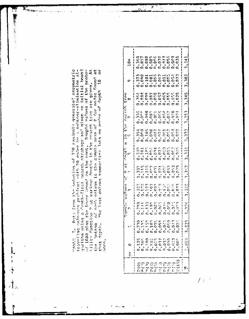
I t4 c. m w~ c -- ,L ,m I-

o C000 0CCOC I (

C- 4 * * * * * .S1 'I 14.4JL I

L4 0 = I M 0.Q r'3,-4, -I r" r-4Ll I' (NC r- 0. I COC, V:L L V, 1 0

. O M , 4 C)0 C . 00 1C

>,-.i oo ooocoo1 o I ri1 r- . . ..C " I(C: J. )4JC ) U.J-C C) C) a - C) c, c I m

t...- v. I d

I - CD- ,0 a c 0 C c I mc V=' c. r4. A) I , . . . . . . . . . I,

4-C 1. cC- aoCoc ----

. C U t. -

c C L . . . -r -C.c, C, : ( c f

w V V, .C CC C k; CC.:C: C:C~ 4 ' (" 0 7 .'L: :'VIC

V- M,. 1- 4 ccc+: (.-- cg': "= g c ,p

4, .IZ . .

. t. CD C CV 0 CC- 4C 0

L) C

" r -c(,

c C:E (' c to c r "C- C- r- L, - --r Ir

: C r .~ .( . . . .

SC0 -C CD C) -C- C 0 .C I el-C, lU... C4: r? ~ ' j0 C C CC CC r-k' -

CC C: EC

c':Z "." CI I

MC . c C.0i 0n- C~-~ L I m

*-.~- C CC 1; 1 I .-- C C:C C

C- C' .r-7 rL t = C E Il l ,c: ,C I

C~ . W C C. C4 i C .'~ C: C- e" v -. (--' C.)

C -C* C r C ' C cl cC I "

C C C C( C. I-rC' (I C

C! CC C'. -CCC

C. 4-1.C'. C' C C C !C O k' I !

S.C ,J1I C "L"C : CL'W 1'I' C ,

V. t.. rN C' - -- C. CN.-f-- -0 C 0 0 1~~ .. .& .. . .C.OC C . .CIt .

..C 4-' f f . C L - C. C. C~) C I C

h 'DC C C c*r"*'~ C C t-X--- C. . .. 0 C . . . C . . C .

lIt

that (1) or (4) is a lower bound , P(O) (the probability that

a randomly picked node in a randomly picked search tree has

zero sons) or, as noted in [Rinnooy Kan and Lenstra 1978), that

O(nc) for any constant c is a lower bound on P(O). This im-

portant result is the object of current research.

For some time now it has been taken as a general guide

that if an algorithm runs in polynomial time then it is a

tractable problem. If the algorithm runs in superpolynomial

time then it is intractable. So far no polynomial time algo-

rithm has been found for any NP-complete problem, so they are

considered intractable. But the NP-complete (and NP-hard)

problems are intractable only in terms of a worst-case bound;

no known algorithm is guaranteed to halt with a solution within

a polynomial amount of time at present. Here though, we have

in the traveling salesman i:-oblem an NP-complete problem which

seems to be solveable on the average in polynomial time. Thus

many instances of the traveling salesman problem can be tract-

ably solved but a few hard instances of the problem cause in-

tractable behavior. The existence of such problems takes some

of the sting from the possibility that PiNP. One might reason-

ably ask whether all NP-complete problems are solveable in po-

lynomial expected time. In fact we might define a new class of

problems called EP which are solveable in polynomial time on

the average. Certainly P EP and it seems that the traveling

salesman problem is in EP. Goldberg (Goldberg 1979] has re-

cently shown that the satisfiability problem seems to be solve-

able in polynomial expected time. A proof that a problem wGNP

-82-

I ... *_,..

is not in EP constitutes a proof that PONP since P is a subset

of EP. The problem of course with this definition of EP is the

need to define an appropriate probability measure on a problem.

Pathological probability measures can be found which emphasize

the hardest instances Of a problem (thus making the problem

seem hard), or emphasize the easiest instances (making the

problem seem easily solveable). Goldberg chose the reasonable

course Of showing that the satisfiablity problem is solveable

in polynomial expected time under several different probability

measures on the problem. So a meaningful definition of EP

awaits further insight into what we mean by a natural or rea-

sonable probability measure on a problem.

In order to predict some of the properties of a depth-

first search on traveling salesman problems, we need a way of

estimating the probability function for the arc costs, Q. We

have found empirically that Q is estimated by the geometric

function

where n is the size of the class of problems. Table 3 compares

some sample mean time complexity statistics for randomly gen-

erated traveling salesman problems solved using a depth-first

search with estimates generated by the function ET introduced

in chapter 6. The randomly generated problems were given an

I. initial bound of 1000 (actually 1000 + lower bound on the ini-

tial feasible set) and the recurrence relation for ET was corn-

puted out to ET(1000). We used (8) for Q and our formulas (4)

-83-

and (5) for P in computing ET, in the column marked ET(1000).

Note that ET(1000) using this P function underestimates the

sample mean. According to our investigation of the best-

bound-first search strategy, we need an upper bound on IF and a

lower bound on P(O) in order to get an estimate which bounds

our sample mean from above. While 'F computed from (4) and (5)

is a good estimate for the mean branching factor over all root

nodes, it does not seem to be a good enough bound on the aver-

age branching factor at other depths according to Table 2. We

obtain good upper bounds by amending P as follows: Halve P(2)

and distribute the difference over P(3), P(4), ... , P(Ln/21).

We retain P(O) = e/n. In this way the mean of F has been in-

creased and the lower bound on P(O) remains. The bounds ob-

tained using this P function in ET are given in the column la-

beled ET'1000) in Table 3.

Theorem 6.3 predicts that the expected size of the search

tree in a depth-first-search grows essentially linearly as a

function of the length of the leftmost path in the search tree.

At the same time that we found the sample mean search tree size

of random traveling salesman problems above, we sampled the

search tree size as a function of the length of the leftmost

branch of the tree. This data is presented in Table 4 and

grapnically in Figure 7.1. The data in Figure 7.3 clearly

shows the linear growth of the mean search tree size for as far

as the sample means are meaningful.

-84-'1

. ... . ' .. .. ... .. ..- . , .. .. ! a!... .. I p... ..... -. .. W .a . W ... . .. .r ...

12TABLE 3. Data from the solution of randomly generated travel-ing salesman problems by a subtour-elimination algorithm usinga depth-first-search strategy and given an initial bound of1000 (1000 above and beyond the lower bound on the root). Thisdata is compared with estimates computed from our model.

Samplemean Sample Stack

Size No. of search ET ETI mean depthof problems tree bound bound stack bound

problem solved size -1000 -1000 depth eq. 6-18

10 1000 10.36 11.06 13.45 2.98 3.68 I15 1000 35.82 30.03 38.61 4.83 5.52 120 790 81.85 64.40 88.72 5.50 7.36

TABLE 4. Data from randomly generated traveling salesman prob-lems giving the mean time complexity as a function of thelength of the leftmost path in the search tree.

Mean search tree size when the leftmost ISize No. of branch has length kof problems I

problem solved Ik=O 1 2 3 4 5 6 7 8 9 10

10 1000 1 5 12 20 27 36 43 51 ...15 1000 1 14 35 48 72 89 99 111 125 145 ...20 780 i1 17 35 85 94 128 160 182 207 299 ...

I.

1-85-

I . .P WW I I.. .. . . .

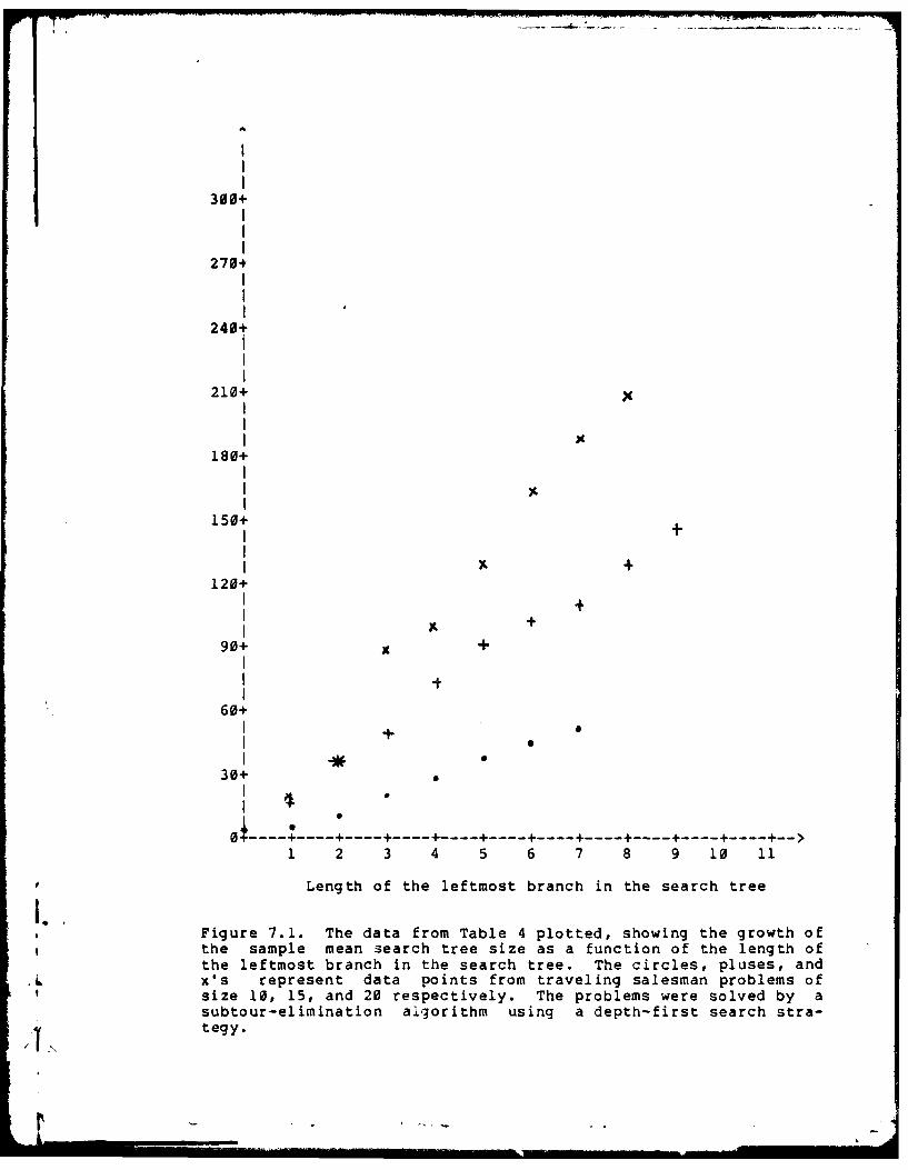
300+

2704

240+

210+

x

180+

Y.

150+ -

I 'IA

120+++

90+ x +

60++

I6I

30+

I0

1 2 3 4 5 6 7 8 9 10 11

Length of the leftmost branch in the search tree

I.I

* Figure 7.1. The data from Table 4 plotted, showing the growth ofthe sample mean search tree size as a function of the length ofthe leftmost branch in the search tree. The circles, pluses, andX's represent data points from traveling salesman problems ofsize 10, 15, and 20 respectively. The problems were solved by asubtour-elimination algorithm using a depth-first search stra-tegy.

Conclusions

Chapter 8

We have studied a model of branch and bound algorithms

and derived expressions for the mean space and time require-

ments for several search strategies. It has been shown that in

our model the best-bound-first search strategy is optimal in

terms of our measures of time and space complexity. The

results we have obtained are essentially order of magnitude

results and it may turn out in practice that the constants as-

sociated with the order of magnitude for a given algorithm make

a difference as far as the choice of search strategy. In a

best-bound-first search a unit of storage may be quite large

if, for example, we need to store an entire matrix as in an in-

teger linear program, since enough information must be stored

in order to restart the search from each unexplored node. On

the other hand, in a depth-first search, the context of the

search is stored in the ancestors of a node, so comparatively

little information need be stored per node. For this reason

the best-bound-first search strategy, although widely recog-

nized as optimal in terms of time complexity, is viewed as ex-

cessively space-consuming. Another complaint against the

* best-bound-first search strategy is the inefficiency caused by

the bookkeeping involved. But there are efficient data struc-

-87-

I' -~ '

AD AC81 (.08 NAVAL POSTGRADUATE SCHOOL MONTEREY CA F/6 12/1ON THE COMPUTATIONAL COMPLEXITY OF BRANCH AND BOUND SEARCH STRA-ETC(U)NOV 79 0 R SMITH NSF-MCS?4INA'45

UNCLASSIFI1ED NPS52-79-004 NL

tures and associated routines for their manipulation available

now which can be used to implement this strategy; one# men-

tioned in chapter 2, being the priority queue [Aho, Hopcroft,

and Ullman 19741. Of the roughly 45 minutes of CPU on an IBM

370/165 spent in producing the data of table 1, less than 6

seconds were spent maintaining the priority queue. Breadth-

first is not usually a practical choice of search strategy for

branch and bound algorithms because it has the disadvantages of

best-bound-first and depth-first without their advantages.

Breadth-first is like best-bound-first in that all nodes in

memory are effectively the roots of different search trees and

for each node all information neccesary for starting up the as-

sociated subproblem must be stored. This means that breadth-

first search has a large constant associated with its space

complexity. On the other hand it is like a depth-first search

in that it is easy to construct a tree for which a best-bound

search explores less nodes than breadth-first search. So it is

nonoptimal in terms of time complexity. A breadth-first search

is reasonable however when it is known or suspected that the

optimal solution is found at a shallow depth.

Our model is particularly suited for modelling relaxation

procedures, where there is some chance that any node in the

search tree of a random problem from a class may produce a

feasible solution. The success of the assignment problem re-

I. laxation for solving assymetric traveling salesman problems and

Held and Karp's 1-tree relaxation for solving symmetric travel-

ing salesman problems suggests that the search for polynomial

-88-

G o

expected time algorithms for solving hard combinatorial prob-

1; ~lems might beg' .,.jking for suitable relaxations and fast

algorithms for - ng them. The search for fast approximate

- algorithms for hard combinatorial problems can also benefit

* from the use of relaxations of a problem. A relaxed solution

to a problem may have many of the components of an optimal

feasible solution. A heuristic restructuring of the relaxed

solution might produce a feasible solution of near optimal

-89-

APPENDIX

Several of the results of this thesis have been formulated

as somewhat complex recurrence relations. In this section we

show how two of these recurrence relations can be broken down

into simpler relations which aid in the computation of their se-

quences.

In chapter 3 the function 0 was introduced in the form

i . i s1 - I 0(k) = I P(j)*[1 - I I Q(c)0(s-c)]J (1)

k= j=1 s-i c-i

with boundary condition 0(0) - P(O).

LetS

E(s) - 5 Q(c)O(s-c),C-i

i sG(i) = 1 - I I Q(c)O(s-c)

S-1 C-i

i- i - 5 E(s) - G(i-1) - E(i),

s-i

B(i) - I P(J)G(i) J ,J=16(1) = s(i- ) - (i).

I. Note that B(i) - 1 - O 0(k), therefore B(i-l) - B(i) 8 0(i). Ink-0

terms of these functions the computation of 0 proceeds as given

in the high level algorithm of figure A.1. For some Q functions,_0

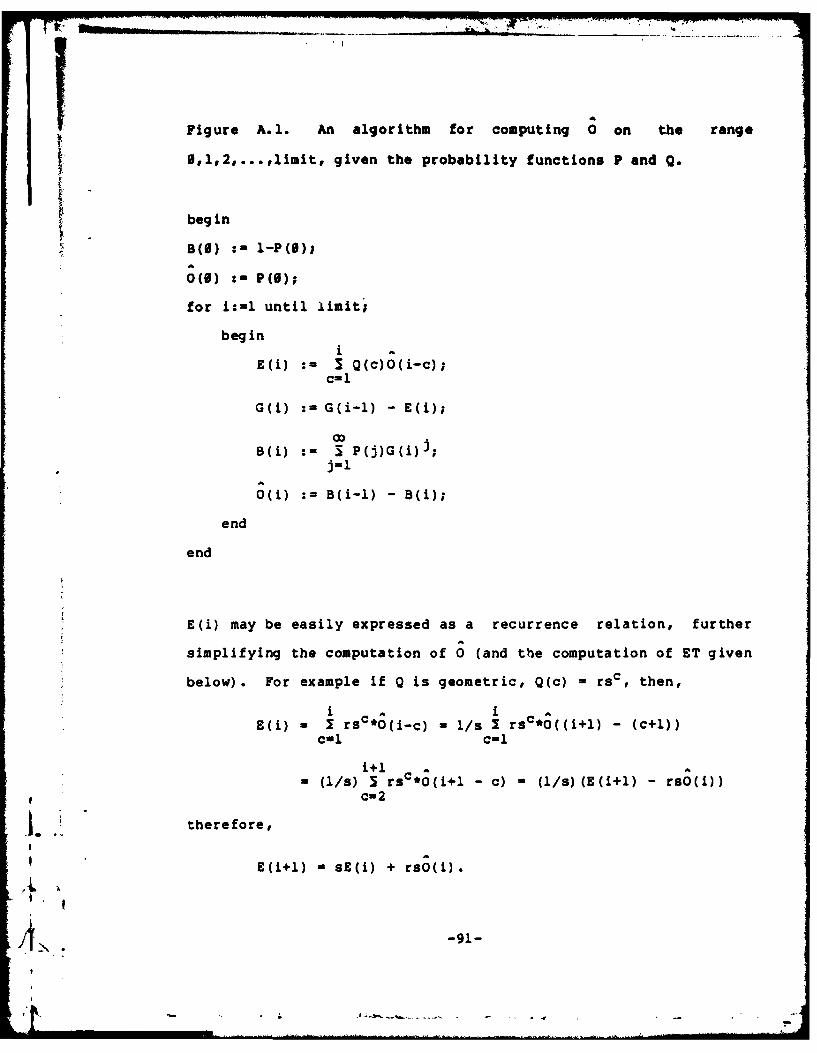
Figure A.l. An algorithm for computing 0on the rang.

t S~,2,..,liitgiven the probability function. P and Q.

begin

B(S) :m1-F(S);

0(0) : (S);

for i:-1 until limit;

begin

E(i) : 3 Q(c)O(i-c);c- 1

B(i) : 3 P(j)G(i)];j=l

end

end

E(i) may be easily expressed as a recurrence relation, further

simplifying the computation of 0 (and the computation of ET given

below). For example if Q is geometric, Q(c) - rsC then,

i A IE(i) - I rsc*( c) - 1/s I rsc*0((i+l) -(C+l))

cul c-1

i+l- (11s) 5 rsc*O(i+l -c) -(l/s)(E(i+l) -rs0i)

* c- 2

therefore,

E (i+l) -sE M) + rso M).

IN -91-

T

The recurrence relation for ET(b) introduced in chapter 6 can be

simplified in a similar manner. ET(b) has the form

ET(b) - 1 + P(j) 5 Wd(b,i) (2)jol i1=

where Wd(b,i) =

c m* m Q(cl) ... Q(ci)O(ml)*..(mil1)*cil ci~l m1 -0 mi 1 l=0

*ET(min~b,c1 +m 1c 2 +m 2 ,... ,ci-l+ltl} -ci) (3)

Essentially, Wd(b,i) has the form

Wd(b,i) = ; R(b,i,k) ; Q(ci)ET(k-ci) (4)k-l ci=l

where R(b,i,k) = probability that k = min{b,c 1 +1 1 1 .. •

,c il +1 il}. (the term c.+l is the cost of the least cost leaf

in the jth subtree below the root; c.f. Figure 3b). In other

words, k is the value of the bound immediately after the i-l s t

subtree has been explored. R(b,i,k) may be formulated easily as

follows: We have 2 cases, either k-b or k<b. The probability

that k-b is

R(b,i,b) = Pr(c 1 +l>_b)*Pr(c 2 +1 2 >_b)*...*Pr(ci_ 1 +li_l>b)

Again let

E (s) - Q Q(c)O(s-c)C-1

k-l s

G(k) - 1 - I I Q(c)O(s-c)

k-l- 1 - s E(s) = G(k-l) - E(k-1).

sal

-92-

N

Here G(k) - Pr(c+l>k) and E(k) = Pr(c+l - k),, so

R(bi,b) - G(b) (5)

The other case we need to consider occurs when one of the

subtrees contains a least cost leaf which improves the initial

bound b. The probability that the bound has the value m is the

probability that one of the subtrees has a least cost leaf of

cost m and the rest have least cost leaves of cost > m, thus not-

icing that each of the i-i subtrees may contain the least cost

leaf we have,

R(b,i,m) - (i-1)*E(m)*G(m)i 2 (6)

Substituting (5) and (6) into (4) we getb-11- 1Wd(b,i) - b (i-i)E(k)G(k)i 2 D(k) + G(b) iD(b)

k-i

kwhere D(k) - I Q(c)ET(k-c). Further, letting

c-1

b-1H(b,i) - 5 (i-l)E(k)G(k)i 2 D(k)

k-i

-H(b-1) + (i-i)E(b-i)G(b-l)i- 2D(b-1) (7)

we have

Wd(b,i) - H (b,i) + G(b) i-lD(b).

Looking again at (2), we see that we need partial sums of

Wd(b,i), so let

W(b,i) - 5 Wd(b,i) -W(b,i-i) + Wd(b,i)J01

IiT -93-

I -.. ... -

- W(b, -l) + H (b,i) + G(b) 1 D(b) (8)

Putting all these pieces together, we can compute ET as in Figure

A.2. The infinities which appear in the algorithms of figures

A.1 and A.2 only come into play when P has an infinite range,

i.e., arbitrarily large branching factors are possible. In most

practical classes of problems the branching factor is in fact

bounded. When modeling such cases the infinities are replaced by

whatever bound exists on the branching factor. In an implementa-

tion of this algorithm, the arrays E, G, and D can be replaced by

single variables since only the most recently computed value of

the corresponding array is ever used. Similarly the 2-dimension-

al arrays W and H can be reduced to 1-dimensional arrays.

I-

-94

i/,,,.

Figure A.2. An algorithm for computing ET(b) for the expected

size of a depth-first search tree given P, Q, and 0

begin

F ET(I) 1;l

for all b, W(b,O) 0; I

for all b, H(b,0) 0- ;

G(O) :1

E(0) 0;U

for b :-1 until limit

begin

for i:1l,...,Co

G(b) :G(b-1) -~-)

bE(b) : 5 Q(c)0(b-c);

Calb

D(b) : 0(c)ET(b-c);c-i

for i:1l until co;

W(b,i) :- W(b,i-1) + H(b,i) + Gb b

ET(b) :1 + 5P(j)W(b,j);J-1

end

end

-95-

References

Aho, A.V., Hopcroft, J.E., and Ullman, J.D. (1974), The Designand Analysis of Algorithms. Addison-Wesley, Reading, MA,7I974.

Beardwood, J. Halton, J.H., and Hammersley, J.M.(1959), TheShortest Path Problem Through Many Points. Proc. Camb. Phil.Soc., 55(1959), 299-327.

Bellman, R.E. (1957), Dynamic Programming. Princeton Universi-ty Press, Princeton, NJ, 1957.

Bellmore M., and Malone, J.C.(1971), Pathology of TravelingSalesman Subtour-Elimination Algorithms. Operations Research19, (1971), 278-307.

Bellmore, M., and Nemhauser, G.L.(1968), The Traveling SalesmanProblem: A Survey. Operations Research 16, (1968), 538-558.

Eastman, W.L. (1958), Linear Programming with Pattern Con-straints. Unpublished Ph.D. Dissertation, Harvard Univ., Cam-bridge, MA, 1958.

Feller, W. (1950), An Introduction to Probability and itsApplications, Vol. T. John Wiley &-sons Inc., New York, -J,1950.

Fillmore, J.P., and Williamson, S.C. (1974), On Backtracking: ACombinatorial Description of the Algorithm. SIAM J. of Comput-ing, Vol. 3, No. 1, March 1974, 41-55.

Fox, B.L., Lenstra, J.K., Rinnooy Kan, A.H.G., and Schrage,L.E. (1978), Branching from the largest Upper Bound. EuropeanJournal of Operational Research 2, (1978), 191-194.

Garfinkel, R.S. (1973), On Partitioning the Feasible Set in aBranch and Bound Algorithm for the Assymetric Traveling Sales-man Problem. Operations Research 21(1973), 340-343.

Garfinkel, R.S., and Nemhauser, G.L. (1972), IntegerProgramming. John Wiley, New York, NY, 1972.

Goldberg, A. (1979), Average Case Complexity of the Satisfia-bility Problem. Proceedings of the Fourth Workshop on Automat-ed Deduction, Austin, Texas, 1979, 1-6.

-96-

- %.,~~-

Golomb, S.W., amd Baumert, L., (1965), Backtrack Programming.JACM 12(1965), 516-524.

Harris, T.E. (1963), The Theory of Branching Processes.Springer-Verlag, Berlin, 1963.

Hart, P., Nilsson, N.J., and Raphael, B., (1968), A FormalBasis for the Heuristic Determination of Minimal Cost Paths.IEEE Trans. System ScL. Cybernetics, ssc-4, 1968, 100-107.

Held, M., and Karp, R.M. (1971), The Traveling Salesman Problemand Minimum Spanning Trees: Part II. Mathematical Programming1, pg 6-25, 1971.

Ibaraki, T. (1976), Theoretical Comparison of Search Strategiesin Branch and Bound Algorithms. International Journal of Com-puter and Information Sciences 5, 4(1976), 315-344.

Ibaraki, T. (1977), The Power of Dominance Relations in Branchand Bound Algorithms. J. ACM 24, 2(1977), 264-279.

Ibaraki, T. (1978), Branch and Bound Procedure and State-SpaceRepresentation of Combinatorial Optimization Problems. informa-tion and Control 36, (1978), 1-27.

IBM Mathematical Programming System Extended (MPSX) Mixed In-

teger Programming (MIP) Program Description (1971), TechnicalPublication SH20-0908-1, White Plains, NY, 1971.

Ignall, E. and Schrage, L. (1965), Application of the Branchand Bound Technique to Some Flow-Shop Scheduling Problems.Operations Research 11, pg 400-412, 1965.

Jordan, C. (1950), Calculus of Finite Differences. ChelseaPublishing Co., New York, NY, 1950.

Kanal, L.N. (1978), State Space Models for Pattern Recognition.Laboratory for Pattern Analysis, Univ. of Maryland, CollegePark, MD 20742, 1978.

Karp, R.E. (1972), Reducibility Among Combinatorial Problems.in Complexity of Computer Computations. R.E. Miller and T.W.Thatcher, eds., -Tenum Press, New York, NY, 1972, 85-104.

Karp, R.M. (1976), The Probabilistic Analysis of Some Combina-torial Search Algorithms. in Proceedings of the Symposium onNew Directions and Recent Results in Algorithms and Complexity.KcA-ademic Press,7I176.-

Klee, V., and Minty, G.J. (1970), How Good is the Simplex Algo-rithm? Mathematical Note No. 643, Boeing Scientific ResearchLaboratories, 1970.

A. Knuth, D.E. (1968), Fundamental Algorithms: The Art of Computert I

' -97-

. . .. .....mom

Programming 1, Addison-Wesley, Reading, MA, 1968.

Knuth, D.E. (1974), Estimating the Efficiency of Backtrack Al-gorithms. Mathematics of Computation, 29(1975), 121-136.

Knuth, D.E., and Moore, R.W. (1975), An Analysis of Alpha-BetaPruning. Artificial Intelligence, 6(1975), 293-326.

Kohler, W.H., and Steiglitz, K. (1974), Characterizations andTheoretical Comparison of Branch and Bound Algorithms for Per-mutation Problems. J. ACM 21, 1(1974), 140-156.

Kohler, W.H., and Steiglitz, K. (1975), Enumerative and itera-tive Computational Approaches, in Computer and Job-ShopScheduling Theory, E. Coffman, Ed., Chapter 6, Wiley In-t-ersc-ence, New York, NY, 1975.

Lawler, E.L., and Wood, D.E. (1966), Branch and Bound Methods:A Survey. Operations Research 14, 4(1966), 699-719.

Lawler, E. (1976), Combinatorial Optimization: Networks andMatroids. Holt, Rinehart, and Winston, New York, NY, 1976.

Lehmer, D. (1959), The Machine Tools of Combinatorial Mathemat-ics. in Applied Combinatorial Mathematics. Ed. Beckenbach,John Wiley Co., 1964, 5-31.

Lenstra, J.K., and Rinnooy Kan, A.H.G. (1978), On the ExpectedPerformance of Branch and Bound Algorithms. Operations Research26, 2(1978), 347-349.

Lin, S. (1965), Computer Solutions of the Traveling SalesmanProblem. Bell System Technical Journal, Vol. 44, 1965,2245-2270.

Liu, C.L. (1968), Introduction to Combinatorial Mathematics.McGraw-Hill Book Co., New York, NY, 1968.

Luenberger,D. (1973), Introduction to Linear and NonlinearProgramming. Addison-Wesley Pub. Co., Reading, MA, 1973.

Mode, C.J. (1971), Multitype Branching Processes: Theory andApplications. American Elsevier Publishing Company Inc., NewYork, NY, 1971.

Mitten, L.G. (1970), Branch and Bound Methods: General Formula-tion and Properties. Operations Research 18, (1970), 24-34.

Morin T.L., and Marsten, R.E. (1976), Branch and Bound Stra-tegies for Dynamic Programming. Operations Research 24, pg611-629, 1976.

Morin T.L., and Marsten, R.E. (1978), A Hybrid Approach toDiscrete Mathematical Programs. Mathematical Programming 14,

-98-

I - --

pg 21-40, 1978.

Munkres, J. (1957), Algorithms for the Assignment and Transpor-tation Problems. J. Soc. Indust. Appl. Math., Vol 5, No. 1,March, 1957, 32-38.

Nilsson, N.J. (1971), Problem Solving Methods in ArtificialIntelligence. McGraw-Hill, NY, 1971.

Papadimitiou, and Steiglitz (1977), On the Complexity of LocalSearch for the Traveling Salesman Problem. SIAM J. of Computing6, pg 76-90, 1977.

Parzen, E. (1962), Stochastic Processes. Holder-Day Inc., SanFrancisco, CA, 1962.

Rabin. M.O. (1976), Probabilistic Algorithms. in Proceedingsof the Symposium on New Directions and Recent Results inAlgorithms and Complexity. Academic Press, l976.

Reingold, E.M., Neivergelt, J., and Deo, N. (1977),Combinatorial Algorithms: Theory and Practice. Prentice-Hall,Englewood Cliffs, NJ, 1977.

Reiter, S., and Sherman, G.S. (1965) Discrete Optimizing. SIAMJournal 13, No.3, 1965, 864-889.

Riordan, J. (1859), An Introduction to Combinatorial Analysis.John Wiley & Sons Inc., New York, NY, 1958.

Rinnooy Kan, A.H.G. (1976), On Mittens Axioms for Branch andBound. Operations Research 24, 6(1976), 1176-1178.

Rinnooy Kan, A.H.G. (1974), On Mittens Axioms for Branch andBound. Working Paper W/74/45/03, Graduate School of Manage-ment, Delft, The Netherlands, 1974.

Salkin, H.M., and De Kluyver, C.A. (1975), The Knapsack Prob-lem: A Survey. Naval Research Logistics Quarterly 22, pg127-144, 1975.

Shapiro, D.M. (1966), Algorithms for the Solution of the Op-timal cost and Bottleneck Traveling Salesman Problems. Unpub-lished Sc.D. Thesis, Washington University, St. Louis, Mis-souri, 1966.

Smith, T.H.C., Srinivasan, V., and Thompson, G.L. (1977), Com-putational Performance of Three Subtour Elimination Algorithms

° for solving Traveling Salesman Problems. Annals of DiscreteMathematics, Vol. 1, 1977, 495-506.

IL Weiner, P., Savage, S.L., and Bagchi, A. (1973), NeighborhoodSearch Algorithms for Finding Optimal Traveling Salesman Toursmust be Inefficient. Proc. of the Fifth STOC Conference, 1973,

'I ,99-

iI l i I...... .

207-213.

-100-

INITIAL DISTRIBUTION LIST

Defense Documentation Center 2Cameron StationAlexandria, VA 22314

Library 2Code 0142Naval Postgraduate SchoolMonterey, CA 93940

office of Research Administration1Code 012ANaval Postgraduate SchoolMonterey, CA 93940

Assistant Professor Douglas R. Smith 25Code 52ScNaval Postgraduate SchoolMonterey, CA 93940

National Science Foundation 2Washington, D. C. 20550

T :-.101