Naval Research Laboratory , 557Washington, DC 20375-532011 I 11,1 lll f ll 111111l1111

NRL/MR/5309--93-7316

I

RADARC HF Ionospheric PredictionII Program for OTH RadarI

ID. L. LUCAS T.CG. S. PRINSON 2R ALCr,

Lucas Consulting S L ; 22 1993

J. M. HEADRICK A I.IJ. F. THOMASON

i Radar Division

II

September 3, 1993

IIII

AplrOVed for public release; distribution unlimited. 9 - 1 4- -' - 93-21942 -lllll~illl~i

2, . P.

IREPORT DOCUMENTATION PAGE Form ApprovedI OMB No. 0704-0188

Putblic spoitO Iurdoetfor li llction of riformation i eatinated to vevraOl I howr pe irwt. indttig the t fa. fo•r rvtwe u eu ctin tor g, metv data eourm.oIwm. dm e dneded. ecmpemd inWgc w rmvewi the w elction of kInomaim. Send cmrm~uat ordug •aneti or aw othe tof• tecolection of ironum lding Wi" gotom for educig tNo burden, to Weeenoten loadqueutore servicee. Directfoate rm Opertiorm un lapos. 1216 JefforsonDwie Highwe,. Site 1204. Arlington. VA 222024302. oad to the Office of MUanqemraennd sudget. Papework Reduction Project 10704-01 $81, Whinotlnton. DC 20603.

1. AGENCY USE ONLY (Leave Blank) 2. REPORT DATE 3. REPORT TYPE AND DATES COVERED

September 3, 1993S 4. TITLE AND SUBTITLE 5. FUNDING NUMBERS

RADARC HF Ionospheric Prediction Program for OTH Radar PE - 63741DDN - 291-215

I 6. AUTHORIS)

D.L. Lucas,* G.S. Prinson,* J.M. Headrick, and J.F. Thomaon

I 7. PERFORMING ORGANIZATION NAME(S) AND ADDRESS(ES) B. PERFORMING ORGANIZATIONREPORT NUMBER

Naval Research LaboratoryWashington, DC 20375-5320 NRL/MR/5309-93-7316

9. SPONSORING/MONITORING AGENCY NAME(S) AND ADDRESS(ES) 10. SPONSORING/MONITORINGAGENCY REPORT NUMBER

Electronics Systems Space and Naval Warfare Systems Command5 Eglin Street, PMW-148Hanscom AFB, MA 01731-2121 Washington, DC 20363-5100

I i 11. SUPPLEMENTARY NOTES

*Lucas Consulting

I 12a. DISTRIBUTION/AVAILABILITY STATEMENT 12b. DISTRIBUTION CODE

Approved for public release; distribution unlimited.

13. ABSTRACT IMaximum 200 wooda)

A model for predicting the performance of an over-the-horizon high frequency (HF) radar is described. The program can alsobe used for management of an existing radar or for HF broadcasting assessment. When the radar parameters, such as power,antenna, and frequency are given the program predicts the signal-to-noise, ground clutter-to-noise, ionospheric spread Dopplerclutter-to-noise, and received power as a function of range from the radar site.

The report is intended to provide the reader with a general description of the prediction model and to show those mathematicsand procedures which are upgraded from NRL Report 2226. The procedures should provide the OTH radar engineers with

information to execute the program for studies or evaluation of existing or planned radars.II

3 14. SUBECT TERMS 15. NUMBER OF PAGES

HF Skywave radar peformance prediction 236Ionospheric models 16. PRICE COODEOTH radar

17. SECURITY CLASSIFICATION 18. SECURITY CLASSIFICATION 19. SECURITY CLASSIFICATION 20. LIMITATION OF ABSTRACTOF REPORT OF THIS PAGE OF ABSTRACT

UNCLASSIFIED UNCLASSIFIED UNCLASSIFIED UL

NSN 7540-O1-290-.65W Stinorpr Form 2t Sev. 2-89Preewlbed by ANDs SMd 230-1l

Si 291-102

II3 Table of Contents

I List of figures vi

List of tables vini

I PART I: Theory and mathematics of RADARC

3 1. Introduction ......................................... 3

2. Background ......................................... 4

I 3. General description of the radar model ....................... 6

3 4. Virtual height ionogram technique and data ..................... 7

5. Generating a virtual height profile ......................... . 10

5.1 The D-region 10

3 5.2 The E-Region 10

5.3 The F-Region 12

6. Electron density profile model ............................ 16

3 6.1 D-E Region 17

3 6.2 F2-Layer 18

6.3 E-F2 Transition Region 18

I 6.4 Fl-Layer 19

3 7. Virtual height ray path model . ........................... 20

7.1) Virtual height ionograms 20

8. Reflectrix model . ................................... 23

9. Ionospheric loss model . ............................... 28

I

I

10. D-E Region ionospheric losses ............................ 30

11. Loss for propagation above the . .... ...................... 36

12. Sporadic-E losses ...................................... 38

13. System loss .......................................... 39

14. Antenna gain ......................................... 41

15. Ground reflection loss ................................. 41 116. Environmental noise ................................... 43

17. Backscatter amplitudes and ray-paths ....................... .. 45

18. Summary ................ ................. 47 1PART II: Users guide to RADARC input/output 51. Input .............................................. 51

1.1 Files used by RADARC 51

1.2 Details of FORM 1 user input 53

2. Output. ............................................ 65

2.1 FOR010: Single frequency rayset tables 65

2.2 FOR030: Vertical ionograms 72 12.3 FOR030: Combined frequencies range plot 74

2.4 FOR030: Oblique ionograms 78

2.5 FOR030: Combined mode/frequency rayset tables 81 I2.6 FOR032: Single frequency range plots 83

2.7 FOR032: Single frequency angle coverage 86

2.8 ALLMODES.DAT: Combined envelope rayset tables 89

I

U

2.9 FOR034: Diagnostics 91

SPART III: FORTRAN implementation details

1. Program description of RADARC .......................... 95

1.1 List of routines; short description 96

1.2 Chart of RADARC calling structure 101

3 1.3 Individual module implementation information 104

List of References ......................................... 224

ISAcce- 'ion For

M! I I s CR,",R .L L..F ,c. :'•d [.

.......... ... .. ... ..... .... .. ...........

6. . ... ......................... .. . . . . .

DI

IV

U 0c~,.-1 ! '" 'L

II

I

I

II

List of Figures I

PART I: Theory and mathematics of RADARC 5Figure 1 True Height profile using three overlapping parabolas. 8

Figure 2 True height profile and virtual heights 8 3Figure 3 Contours of the ratio hmF2/ynF2- top high SSN, 15

bottom low SSN. 3Figure 4 Gaussian integration 22

Figure 5 Oblique raypath geometry for three layers. 24

Figure 6 Reflectrix. 27

Figure 7 Skywave non-deviative absorption component of system 32

loss.

Figure 8a Ground reflection loss for poor earth (E=4 ;b5=.00l) 42 5Figure 8b Sea water reflection loss (E=80; 5=10). 42

Figure 9 Numerically mapped values of atmospheric radio noise 43 3at 1 MHz, F. (dB > (Ktob), for Dec-Jan-Feb, 00-04 LMT.

Figure 10 Frequency dependence of the atmospheric radio noise 44 1(F•) for 00-04 LMT, Dec-Jan-Feb.

Figure 11 Man-made noise as a function of area population (-dBW) 45

Figure 12 Example raypaths of the backscatter signal 46

PART II: Users guide to RADARC input/output

Figure la,b FOR010: Single frequency regular mode rayset tables 68,69 5Figure 2a,b FOR010: Single frequency sporadic E mode rayset tables 70,71

Figure 3 FOR030: Vertical ionograms 73

Figure 4a,b,c FOR030: Combined frequencies range plot 75-77

Figure 5 FOR030: Oblique ionograms, large scale 79 3Figure 6 FOR030: Oblique ionograms, small scale 80

Figure 7 FOR030: Combined mode/frequency rayset tables 82

Figure 8a,b FOR032: Single frequency range plots 84,85 Ivi[

Figure 9a,b FOR032: Single frequency angle coverage 87,88

Figure 10 ALLMODES.DAT: Combined envelope rayset tables 90

Figure 11 FOR034: Diagnostics 92

PART III: FORTRAN implementation details

Figure 1 Chart of RADARC calling structure 101-103

iIIIIII

III "

II

List of Tables

Table I Relationship between vertical data (lonogram) 5and oblique data (Reflectrix) 25

Table II Rayset for a single operating frequency. 26 3Table III Excess system loss (dB) for high (N or S) latitude paths. 29

II

IIIII

IIII

'viii I

PART I

Theory and mathematics of RADARC

RADARC

HF IONOSPHERIC PREDICTION PROGRAM

I for OTH RADAR

I 1.) IntroductionI

The OTH radar prediction model was developed by the Naval Research Laboratory (NRL)

by contract to the Institute for Telecommunication Sciences (ITS) and Lucas Consulting. The

program is designed for use as a tool in predicting or analyzing existing system performance for

OTH radar facilities that use the HF (3-30 MHz) portion of the electromagnetic spectrum and

the ionosphere as a propagation medium. The prediction program can be used in the design and

siting of an HF radar installation as well as in the frequency and scan management of an

operational site. This, however, does not limit the usefulness of program RADARC to radarapplications alone. Organizations interested in HF broadcasting and communication will find that

this prediction program can be used to evaluate many of the pertinent propagation problemsaffecting the reliability of the particular HF facilities. Some of the more common needed

parameters in HF radar, broadcasting and communication operations are the expected limits for

the take-off and arrival angles, height of reflection, area coverage and signal-to-noise ratio

associated with given frequencies and times. Program RADARC predicts the above parameters

among others and enables the user to ascertain revisions necessary in frequency complements,

antenna selection, power requirement and/ or site selection in order to maintain optimum HF

system performance.

This documentation is presented to assist the users of program RADARC to understand its

general flow and to explain the essential calculations in the procedures involved. A continuous

effort is being made to update the model and the procedures employed; thus all portions of the

program are subject to revision.

The model used in the program RADARC for predicting the expected performance of

ionospheric radar systems is the result of the philosophy and work of many investigators and no

attempt will be made to credit all of the sources used. This documentation is intended to be a

description of a computer program for users and not a monograph on HF ionosphericpropagation.

Mumucript apoved July 15. 1993.

1 3

I

2.) Background

This section is intended to provide the reader with a general background used in the basic 3philosophy and development of the program RADARC.

Numerous organizations both governmental and private have been employing high frequencies

to communicate between remote long distance point-to-point stations. It was recognized early [that these types of communication systems were subject to marked variations in performance and

it was hypothesized that most of these variations were directly related to changes occurring in ithe ionosphere. Considerable effort was made in the U.S. as well as other countries to develop

research teams for the purpose of investigating ionospheric parameters and determining their

effect on the nature of radio waves and the associated reliability of HF circuits. The

investigators soon realized that effective ope ation of long distance HF systems increased in

proportion to their ability to predict variations in the ionosphere because it allowed them to select

optimum frequencies, antenna systems, and other circuit parameters that would capitalize on these

variations. With the encouragement provided by these findings it was decided that a great deal

more raw ionospheric data was necessary in order to develop models that could be used to

adequately anticipate ionospheric conditions affecting HF propagation. Worldwide vertical iincidence ionosondes were established and now measure values of f.E, fFl, foF2, etc. as

described in a later section. Worldwide noise measurement records were started and steps were 3taken to record observed variations in signal amplitudes over various HF paths. The results of

this research established triat ionized regions ranging from approximately 80 to 600 Km above 3the earth's surface provide the medium of transmission for electromagnetic energy in the HF

spectrum (3-30 MHz) and that most variations in HF system performance are directly related to

changes in these ionized regions, which in turn are affected in a complex manner by solar

activity, seasonal, and diurnal variations as well as latitude and longitude.

The Radio Propagation Unit of the U. S. Army Signal Corps provided a great deal of

information and guidance on the phenomena of propagation with HF in 1945 by issuing Technical

Report No. 6'. By 1948 a treatise on ionospheric radio propagation was published by the Central 3Radio Propagation Laboratory of the National Bureau of Standards2 . This document outlined the"state-of-the-art" of predicting expected maximum usable frequencies (MUF), depicted practical 3problems of ionospheric absorption and covered in detail acceptable methods of determining the

MUF for any path at any time, and took into account the various possible modes of propagation 3by applying principles which were found to work in practice. The model used to make the MUF

4i

predictions employed the "two control point" method and assumed the ionosphere to beconcentric with reflection occurring only from the regular E- and F2-layers.

In 1950 Laitinen and Haydon3 of the U. S. Army Signal Radio Propagation Agency furtheredthe science of predicting HF system performance by developing empirical ionospheric absorptionequations and combining this with the theoretical ground loss, free space loss, and antenna power

gain so that expected field strengths couid be anticipated for radio signals reflecting from the E-and F-regions considering the effects of solar activity, and seasonal and diurnal extremes. The

accumulative techniques and methods presented in the above-mentioned literature and many otherstudies were then combined to establish effective manual methods for predicting the expectedperformance of HF communication systems; however, these methods were laborious andtime-consuming even if only estimates for the MUF and FOT (.85 MUF) were needed. Toalleviate this problem, electronic computer routines were developed by such organizations asStanford Research Institute4 and the Central Radio Propagation Laboratory3 , all of which werebased upon the established manual prediction methods. The latter program gave the firstcomputerized technique that incorporated the numerical coefficient representation of theionospheric characteristics. However, only the expected MUF and FOT were predicted. In 1962a report was issued outlining a computer routine that used the most recent improvements in the

theory of performance predictions, combining the more predictable ionospheric characteristicswith circuit parameters to calculate expected HF system performance; MUF-FOT, system loss,reliability, etc.(Lucas)6

By 1960, it was recognized that high frequency radar systems could detect targets atconsiderable distances and consideration was given to the idea of applying the already developed

computer programs used to predict the ionospheric effect on HF communication to the HF radar

system. At the outset simple revisions were made to the HF prediction program includingdoubling the ionospheric losses associated with a given point-to-point path.

The predicted signal-to-noise ratios obtained by these modifications were compared with actualbackscatter amplitudes and the results were encouraging. However, there were obviousdeficiencies in the model that appeared immediately. To list a few:

I. Mirror reflection from the E- and F2-1ayers was not satisfactory.

2. The Fl-layer was not included as a separate layer.

3. The sporadic E-layer was not included.4. The take-off angle was not dependent on frequency.

5. Predicted losses were in error when transmission by the E-layer

was nearly specular.

It was possible to revise the prediction model to at least predict all of the above deficiencies.

The development of the parabolic distribution of electron density model laid down in ITSA-I' 6

was a first step. In this model the electron density profile along the path was assumed to be

adequately represented by two parabolic layers, i.e, E and F2. The height of maximum

ionization, semi-thickness, and electron density were derived from locations near the points of

actual reflection along the path instead of the classical "two-control-point" method previously

used in the calculation of the upper limit of frequencies and transmission loss.The program RADARC is a direct descendent of the ITSA-1 model and does consider the E.,

E, Fl, and F2 reflecting regions in the calculation of expected system performance for HF OTHRADAR 7. The mathematics and method of generating the virtual height profile from the three

parabolas is that of IONCAP9 . Other modifications such as the revision to transmission loss at

lower layers, obscuration by the E, -layer, etc. will be discussed in detail in later portions of this

report.

3.) General description of the radar model

The NRL HF OTH model is based upon the large volume of ionospheric data compiled over 3the years by the Institute of Telecommunication Sciences and is in the evolutionary line of the

methods and computer models used in the analysis of communication systems. However, the 3emphasis in the NRL OTH model is on the description of the ionosphere along a great circle

covered by the transmitted signal rather than the description of the electromagnetic environment

at a single point as is the purpose of many other models.The prediction model RADARC is an upgrade of RADARB as described by Headrick,

Thomason, et al'. The mathematics of the geometry and the numerical evaluation of the Icoefficients associated with the ionospheric parameters are not included in this report as they are

thoroughly covered in the above report. The ionosphere representation and development are those

of IONCAP9 and will be explained in detail in later sections. The program is no longer just a

'two control point' prediction routine, but will allow, up to ten control areas sampled any 3reasonable arbritary evenly spaced distance. It will allow calculations of from 1-hop to 4-hops

of propagation by the E,, E, Fl, F2, or mixed modes using take-off angles from 0 to 45 degrees

to sample the coverage area for the specified azimuth from the transmitter. The program will

6 3

IU

calculate the signal-to-noise, earth clutter-to-noise, and the ionospheric spread Doppler clutter

3 as described by Elkins38 '3 9 The program is very versatile with a plain language input file and

highly documented output files, as will be shown in later sections on the input necessary to

3 execute the program and the expected output.

Those readers not interested in the some of the mathematical and physical development of the

3 program should go to part II. The prediction mathematics, data and calculations are summarized

in the following sections. The first sections describe the development of the predicted ionosphere

(h'F trace). The next sections describe the prediction and development of the transmission loss

associated with the predicted virtual ionogram and the later sections describe the methods of

predicting the coverage of the radar using the radar equation and the predicted noise

I environment.The sections that immediatley follow will take you through the prediction routine RADARC,3 the data used to develop the ionospheric representation, the mathematics used in the virtual height

vs frequency trace development, and the prediction of the transmission losses. These sections are

3 from unpublished works of John L. Lloyd, Donald L. Lucas, and George W. Haydon9.

4.) Virtual height ionogram technique and dataIThe prediction technique is a ray-path model using only data available for all values of the

3 solar cycle, all times of the day, all months of the year, and all geographic locations. The

mathematics for describing the ionosphere in virtual height and frequency resembles those of

3 IONCAP9. The model assumes the vertical distribution of electron density with height can be

modelled using a parobolic distribution for each layer. These parabolas are described by using

the predicted critical frequency as the value at the nose and the predicted semi-thickness as its

width. The height of the parabola is assumed to be at the predicted height of maximum. These

parobolas are then overlaid upon each other in true height to form a true height profile of

electron density (figure 1). The corresponding virtual height is found by integrating through this

true height profile (figure 2). The virtual height profile thus generated is now used for all ray-

I path determination and calculation of angles of radiation. Figure 2 should be inspected carefully

as this is the most difficult part of the prediction routine and the most lengthy to explain. Most

3 other calculations depend to some extent on this ionospheric description. The following sections

explain the data and method used to generate the predicted ionosphere.

IU

Z. Is 7

raa

bit

toy".l f'72

VERTICAL VREQU.CT

Figure 1 True Height profile using three overlapping parabolas.

H-EIGHT, kmMVIRTUAL

hI

ymFa

PARABOLIC NOSE3

yMF1 LINEAR (or PARABOLIC) LEDGE

(f~h~) LINEAR, VALLEYI

hmE~ -w-PARABOLIC NOSE

70 k .. ,EXPONENTIAL TAIL

WOE foFt toFa

FREQUENCY

Figure 2 True height profile and virtual heights

Some discussion will be given about each contributing layer as the mathematicsI

8I

U

are explained to help in understanding what is taking place in the ionospheric

3 model development.

IIIIUII

II

II

II

5.) Generating a virtual height profile

The ionosphere exhibits considerable systematic variability. If the minute-to-minute and the Uday-to-day variations within the month are averaged the remaining temporal variations (ie;

diurnal, seasonal, and solar become fairly well behaved and predictable.

It is the purpose of this section to discuss parameters available to describe this quiet Iionosphere and to review the available measurements and associated predictions for each region

of the ionosphere. UAvailable ionospheric parameters, the use of these parameters to predict electron

density profiles, and the use of the profiles to predict the geometry and losses

associated with skywave propagation will be discussed in the sections to follow.

5.1) The D-region

Information on electron densities in the lower ionosphere (50-90 Km) is

very inadequate for use in a prediction model such as this, primarily as

a result of limited observation directed toward prediction use. The technical problems of

observations are formidable, and the interpretation of measurements extremely difficult.

No D-region paramenters are directly included in the prediction model described in this report.The effect of the D-region is accounted for in two ways. First, the electron density distribution

is extrapolated from the E-region using an exponential decrease to the height of 70 Km (Figure 32). Second, the effect of absorption is included in the loss equation. I5.2) The E-Region 3

A large volume of vertical-incidence ionosonde data has been collected over about three solar 3cycles, and many features of the E-region are therefore well known. The minimum virtual height

of the E-region and the variation of maximum electron density within this region as a function

of time and geographic location are readily obtained from the ionograms. The phenomenology

of sporadic-E has been investigated, but classification of sporadic-E types remains unresolved.

The effects of different types of sporadic-E on oblique-incidence radio propagation are not 3established; as a result, the compilation of meaningful statistics to form the basis of predictions

I10 3

11

is difficult.The E-region characteristics that have been systematically scaled from the vertical-incidence

ionosonde records include:If.E The critical frequency of the ordinary component of the E layer;

i.e., that frequency at which the signal from the ionosonde justpenetrates the E-layer.

Ih'E The minimum virtual height of the E-layer, measured at the pointwhere the trace becomes horizontal.

fE, The highest observed frequency of the ordinary component of3 sporadic E (E,).

Wh'E, The minimum virtual height of the sporadic-E layer, measured at

the point where the trace becomes horizontal.IfbE, The blanketing frequency; i.e, the lowest ordinary wave frequencyat which the Es layer begins to become transparent, usuallydetermined from the minimum frequency at which ordinary wave

reflections of the first order are observed from a higher layer.

I The regular E-layer is predicted using three parameters: the monthly median value of criticalfrequency (foE), height of maximum ionization of the layer (hmE), and ratio of h.E to semi-3 thickness (ymE). Worldwide numerical coefficients of monthly median f0E are available forcomputer applications in terms of geographic latitude, longitude, and universal time. The3 coefficients (Leftin)'° were derived from measurements taken during a year of minimum and ayear of maximum solar activity. A linear interpolation is used to obtain estimates at other phasesof the solar cycle. An examination of monthly median h'E observations indicates negligible

seasonal or geographic variations in the minimum virtual height of E-region ionization. A typical

value is 110 km. The D-region ionization is included as an exponential decrease below the E-

layer; an hmE of 110 km and an hmE/y.E ratio of 5.5 are assumed; i.e., ymE = 20 km.Numerical coefficients are also available for each month representing the median and decile3values of f.Es (or foE) in terms of a modified magnetic-dip angle, longitude, and universal time

(Leftin)". These numerical maps are from data taken during periods of solar activity minimumI1 1

II

and solar activity maximum. Linear interpolation is used for other levels of solar activity.

Unless other information is available, the virtual height of the sporadic-E layer is assumed to be 3110 km.

I5.3) The F-Region

The vertical-incidence ionosonde network, with its long series of measurements over much

of the world, provides the basis for F-region predictions (Martyn)"2 . The following parameters

have been systematically scaled from the vertical ionosonde records (Piggott and Rawer)"3 ,

although some stations do not report all of them:

f.F2 The critical frequency of the ordinary component of the F2-layer; 3i.e., that frequency at which the signal from the ionosonde just

penetrates the F2-layer. 3M(3000)F2 The factor for converting vertical-incidence critical 3

frequencies to oblique incidence for a distance of

3000 km via the F2-layer.

fyF1 The critical frequency of the ordinary component of the Fl-layer;

i.e., that frequency at which the signal from the ionosonde just 3penetrates the Fl layer. I

h'F The minimum virtual height of the F-layer; i.e., the minimum

virtual height of the night F-layer and the day Fl-layer. It is 3measured at the point where the F trace becomes horizontal. (In

earlier years the minimum virtual height of the night F-layer was

often combined with that of the day F2-layer, the combined

tabulation being designated h'F2. In these cases, the minimum

virtual height of the Fl-layer, h'Fl, was tabulated separately.)

h'F2 The minimum virtual height of the F2 layer, measured at the point

where the F2 trace becomes horizontal.

I

II

h•F2 The virtual height of the F2 layer corresponding to a frequency f,where f-=. 834 foF2. This is based on the assumption of a parabolic

ionization distribution, which is usually considered justified as anSapproximation to the height of maximum ionization of the F2 layer.

The F2 layer is described by three parameters: monthly median value of critical frequency(f0F2), height of maximum ionization (hmF2), and a ratio of h=F2 to semithickness y.F2.Monthly median values of fF2 and the M(3000)F2 for two solar activity levels are available as

numerical coefficients in terms of a modified magnetic-dip angle, longitude, and universal time(CCIR)7. The solar activity dependence is accounted for by linear interpolation. The height ofmaximum ionization is determined by first estimating the virtual height at 0.834 foF2; i.e., hmF2.The geometric formula used is:I (1)

hPF2 = -176 + 1490/M(3000)F2

The expected accuracy of the formula is within 6 percent (Shimazaki)' 4. The form of equation3 (1) is governed by the geometry of a wave propagating in a spherically symmetricearth-ionosphere medium. The 176 is the bulge of the earth for a 3000 km path. The 1490 isan approximation of the quantity

(l a)

3 S = .417 PT

where P' is the group path (slant range) and k is the usual secant correction factor. The basicequations used are

I fa = f/k secb(1lc)

I f = [M(3000)F2][foF2](1ld)

I sec 0 = 1/2 P'/(hmF2 + 176).

I Let f, = 0.834 foF2. Equation (la) is the secant "corrected" law; equation (lb) is the

definition of the 'M' factor; and equation (1c) is a trigonometric identity. (Snell's law, Martyn's

I3 13

II

theorem, and Breit and Tuve's theorem are all implicit here. Any correction to equation (1)should be in the factor 1490. The height of maximum ionization is then found by removing the 3retardation caused by lower region ionization; i.e.,

IhmF2 = hFF2-R. (2)

The formulas for 'R' (Budden)14 depend upon the electron density profile assumed for the 3lower layers. For example, D-E ionization as a parabolic layer with an exponential decrease at

the lower heights, the E-F valley as a linear profile, and the FI, when present, is assumed to be

a linear or parabolic ledge. The ratio (hmF2/ynF2) is available as a function of the sun's zenith

angle (positive for afternoon, negative for morning), geomagnetic latitude, and solar activity, as

shown in figure 3 (Lucas and Haydon)"6 . These contour were developed from 75th meridian dataof computerized true height reductions of ionospheric recordings (Wright)41 .

The Fl-layer is not always present. When present, it is described by three parameters--the

critical frequency (f0Fl), the height of maximum ionization (hmFl), and the semithickness (y,,F1). 3Numerical maps of foFl are available (Rosich and Jones)"1 . These maps provide fyFl as a

function of solar zenith angle, are continuous throughout the year, and are linear with solar 3activity. The Fl-layer fades out at a maximum value of the sun's zenith angle. The height of

maximum ionization (hmFl) appears to depend upon the zenith angle of the sun and is estimated 3in this report as follows:

hmF1 = 165 + .6428(3

hmFl height of maximum ionization of the F l layer in kilometers IX -zenith angle of the sun in degrees.

The ratio of hMFl to the semithickness of the Fl-layer is assumed to be 4.0. The presence of

the Fl-layer is primarily a function of the sun's zenith angle, but also depends upon time of year, 3a modified magnetic-dip angle, and solar activity level. The values of hmFl and yFl are adjusted

so that the Fl-layer smoothly merges into the other regions. 3It must be noted that the values of h•,Fl and ymFl are tentative and require adjustment,

I"4 3

II

3 0 /_A-

I o I • ,

II'• • ".5

L /, 4.0 / 3.040 __5 '..._ 2.5

W &.0

.5•.43 .25I °0

1 0 3*_

-1180 -10 -140 -120 -100 -S0 -60 -40 -20 0 20 40 0 10 I10 120 140 60 It0MORNING ,* i~fRNtOOII

SUN'S ZENITH ANGLE (#$ -DEGREESI110

_-0 10

.5 A. / 3A 4.5

En 4.04. =

-0 - to0/

15.0 /-

40' 3.00

SUN*S ZENITH ANL •1,)-DMGMEES

Figure 3 Contours of the ratio hmF2/ymF2- top high SSN bottom low SSN.

depending upon the ionization of the F2 layer in the development of an electron density profile.The above ionospheric parameters are selected from those available with emphasis on

obtaining consistent parameters for the generation of an adequate electron density profile forestimating the ray-path geometry of high-frequency skywave signals. Other ionosphericparameters which are available but which are not used include:

Maps of f0F2 with a nonlinear dependence on solar activity are notused because the maps of the associated parameter M(3000)F2 are

15

I

available only with a linear dependence on solar activity.

Neither h'F,F2 nor h'F,Fl maps are used because the frequency Iat which the height applies is not measured and it is impossible to

adjust for lower region retardation. Maps of f0F2, M(3000)F2, and

the ratio hmF2/ymF2 are from the same data base and are

statistically and physically consistent.

Maps of fbEs are not used because values are available only for a

low solar activity.

6.) Electron density profile model

Frequency versus virtual height traces of the ordinary wave as available on vertical

incidence ionograms can be converted into electron density profiles by a standard reduction

program. These profiles, including geographic, diurnal, seasonal, and solar cycle variations, are

generated between heights of 70 km and the height of maximum of the F2 layer, hF2. The

electron density is given by the relationship

(4)

N = 1.24 x 10'OfN2 (

N electrons per cubic meter UfN plasma frequency MHz.

The profile is generated in four steps: D-E region, F2-layer, E-F2 valley, and an Fl ledge.

This form of electron density profile evolved over the years. A fixed reflection height for the

E- and F2-layers was used in the original computer program (Lucas and Haydon). Then

parabolic layers for both the E and F2-layer were used (Lucas and Haydon) 6 and (Barghausen

et al)2". The Fl-layer was added and the profile was generated by taking the maximums of these

intersecting parabolas (Haydon and Lucas)"1 . The resulting profile is then a computerized version

of this manual method of analyzing measured ionograms (Ratcliffe)"9 . In all of these programs,

the electron density is only implicit in the functional form of the equations used for virtual 3heights or ground distance. The method described here gives an explicit form for the profiles

I

I

_ (Figure 2).

6.1) D-E RegionIThe ionospheric parameters assumed available are the monthly median critical frequency of

the E-layer (foE, MHz), height of maximum ionization of the layer (hmE = 110 km), and ratio

of h,,E to semithickness (hmE/yE = 5.5).

The nose (figure 2) of the layer is parabolic fN(h) is the plasma frequency at a

2f,(h) f 2 [1 hmE-h 1 (

height h. The ionization is assumed to decrease exponentially starting at the lower part of the

E region (h..= hmE -.85 ymE), with the constants chosen so the slope of the profile is continuous

at this point. (A discontinuous slope results in a cusp in the virtual-height ionogram derived from

the profile.) The equations are

(6)

f2 (h)=OfE)2F 2 exp[a (h -70.)]

a = 2(hE - h•,)/(.2775 (y.E)2)

= 6.121/yE= .3062, for yE =20

where

3 F 2 = [1. - (.85) 2]exp[-a(hmE -. 85ymE-70.)]

This equation gives a value of fN2 at 70 km as (foE)2 F2. With hmE as 110 km and y, as 20

kin, this profile yields a virtual height of 100 km at .04 (f0E)2 and of 110 km at 0.52

(foE) 2,corresponding roughly to typical measured values.

17

II

6.2) F2-Layer IThe ionospheric parameters assumed available are the monthly median critical frequency of

the F2 layer (fF2, MHz), height of maximum ionization (hmF2, kin), and the ratio of h.F2 to

semithickness of the layer (y.,F2).

(7) I

jý= (f.F2)2 [1*.-( hmF2 ~)2]hmF2-

6.3) E-F2 Transition Region IOnly the total density in this region is modeled, not the shape. This is normally, but not

necessarily, a valley. It is represented by a line from a frequency f. at the F2 layer to afrequency f, at the E layer:

(8) i

fA(h) = fu + (fu -f/)[h - hu)l(hu - h/)] Iwhere U

f= x, foE

f= x, foE

hu hmF2-ymF2 (1.vu-( If F2 2)

hV hmE + YmE(1.-('v IfoE)2)

ITypical values for the constants x., and xv are .98 and .85 16, respectively. If x. = xv= 1, i

I"I i

there is no valley.

6.4) Fl-Layer

The Fl-layer is considered to be a ledge from the F2-layer to the E-F valley (or possibly to

the E-layer). If the Fl ledge exists, it is described by three parameters: the critical frequency

(foFl, MHz), the height of maximum ionization (hmFl, kin), and the semithickness (ymFl, km).

The F1 ledge may be either a linear or a parabolic layer. If the height of maximum ionizationof the Fl ledge is less than the height of the F2-layer at the frequency of fFl, the parabolic layer

shape is used. If the height of maximum ionization of the Fl ledge is greater than the height of

the F2-layer, then the height of maximum ioni-ation of the Fl ledge is reduced to the F2-layer

height. This procedure assures that a cusp in a virtual height trace occurs at the critical frequency

of the F I ledge. The slope, S 1, of the linear layer shape using the F I ledge parameters (f0Fl,

hmFl, yFl) is compared to the slope, S2, of the F2-layer at the Fl critical frequency. If thedifference of the slopes is positive, the linear ledge is used; if negative, the parabolic layer shape

is used.This procedure assures that the F1 ledge will appear in a virtual height trace and that the F1

ledge will gradually disappear into the F2-layer as the difference of the slopes approaches zero.

When this difference is small, the resulting ionogram will be L-shaped.

Also, the Fl-layer, when parabolic, can dominate as f.Fl approaches foF2, as occasionally

happens, especially in the Northern latitudes. The equations are:

(9)

h2 = hmF2 - YmF2F(1 - o(fFl / foF2)2

and slopes

S2 = 2(foF2)2 (hF2-h2)/(ymF2)2

Si = (f )2 /y.F1

for a linear ledge (i.e., h2 < hmFl and S2 < S1)

19

II

fN 2(h) = S1 (h- h2 + y,,,Fl) (

and for a parabolic ledge 3(11)

fN2(h) = (f 0Fl) 2

[1 - ((h,,,F1 - h/)ymF!)21 ISample numerical maps of the variation of plasma frequency with height, geographic location,

and local mean time developed for limited time periods (Jones and Stewart)20 are not applicable

to other time periods. The approximate electron density profile described above uses predictions

of ionospheric parameters now available for all time periods and includes variations with latitude,longitude, local time, month, and solar activity. Both the profile and its slope are continuous

except perhaps at the predicted critical frequencies (see Figure 2). Although the methods are Iprimarily for use with predicted monthly median values, they are applicable to daily ionospheric

parameters. The electron density profile (in tabular form) can be used in ray-tracing programs 3or to generate virtual-height ionograms, or in the propagation prediction programs.

7.) Virtual height ray path model IThis section describes a simple computation method for obtaining all the single-hop ray paths

through an ionosphere described by an electron density profile. It uses the classical relationships 3between the virtual-height ionograms and the oblique path. However, Martyn's equivalence

theorem is used in a "corrected" form as described by Lloyd'. First. the ionogram is obtained

using numerical integration techniques. Then reflectrices are uwý,ined as a single table

incorporating all ray-path information. Finally, the correction to \ r' s theorem and a table

look up and interpolation procedure are used to find the ray sets w IhJ• ih describe the propagation

for a particular operating frequency.

7.1) Virtual height ionograms

Virtual heights for the ordinary trace are found from the electron density profile by

numerically integrating the equation 3203

I I

hr

I ho(12)

where

= 11 - fN(h)/ff,2]'

I f, selected vertical sounding frequency;

ho lowest true height of the profile, i.e., 70 km;

I h virtual height of the profile;

h, true height corresponding to f,;

h true height of reflection;

A' group index of refraction;

3 fN plasma frequency.

The area is found using a Gaussian integration technique (see Figure 4). The effect of thecusp at h can be lessened by using a nonlinear transformation from the interval [h., hi], to [1,

1]. The transformation and integration equations are:

I hj (tr - hd[1 -2-(1 - X)P]

F= L'(hjfm)( " -X)m-'

N

h' ho + (hr-h)(m/2N) E wj 'i'I

hi = true height corresponding to (w, , Xj);

Xj = Gaussian abscissa;

w, = Gaussian weight;

N = number of Gaussian terms (at least 40) for electron density

profiles

I

W!

t I

I -

L0x |

H I' I

t ' I

I

A I Ii

""a ie lo .M

Figure 4 Gaussian integrationA forty-point Gaussian integration was found to be adequate when the electron density profile I

was sampled at true height intervals of 4 km and the vertical soundjing frequencies were selectedat intervals of 0.2 MHz. I

The Gaussian method tends to smooth out the "links" in the resulting ionogram introducedby using a tabular form of the electron density profile. When m- =1, it corresponds to the usual

Gaussian formula for an arbitrary interval.When the F l-layer is not present, a faster integration method is available. The D-E regionI

values are taken from a table which was calculated by the Gaussian integration using hmE = 110

and ymE = 20. The F2 layer is calculated using model segments. 3

II

22

I

8.) Reflectrix model

Skywave radio propagation paths may be described by a set of parameters known as raysets

(Croft)2". For most HF radar and communication applications, this consists of operatingfrequency, takeoff angle, virtual height of reflection, true height of reflection, and ground1 distance. The basic inputs are true and virtual heights as a function of vertical-incidencefrequency.

The ray paths are calculated using the following simplifying assumptions:

1. Horizontal and azimuthal variations in the ionospheric electron density profilesare negligible for each hop (on a multihop path, different sample areas are used).

2. The magnetic field may be ignored.3. The ionosphere is spherically symmetric to the earth.

With these simplifications, the equivalence between a given frequency on an oblique path (fob)and a vertical incidence frequency (fQ) with the same vertical height specified by Snell's law is

(14)

fob= fseco,

where

*, is the angle between the apparent ray path and the normal to the earth atthe true height of reflection.

By simple geometry, the virtual height of the oblique path is related to the

takeoff angle A by (figure 5).

acosA = (a +hh )Sin "(where

A = takeoff angle of the ray,a - earth's radius,

h',= virtual height of the oblique path,

= is the angle between the virtual ray and the normal to the

earth at h',b

N Martyn's theorem for a plane ionosphere specified the ray path by the equality of the virtual

*23

II

/'

Figur ortee I

height of the oblique path, with the virtual height of the ionogram at the equivalent frequency f,.I

For a curved ionosphere, this leads to a consistent error at higher frequencies for thicker layers.The Breit and Tuve theorem states that the time taken to transverse the actual path is the sameas that which would be taken to transverse the equivalent path in free space. Both theorems areI

corrected in the following model by an empirically derived correction (Lloyd)" factor whichdepends only on the electron density profile and the curvature of the ionosphere:

hb-- [hh' -h h'h-h)2]I

fofý a a

Note..h'•, has changed definition.

wherei

f.F2 is the 1=2 critical frequency,h' is the virtual height corresponding to fv,|

/2

UI

h is the true height of reflection

This correction has errors of less than one percent as compared with the distances calculated3 by a ray-trace program based on Haselgrove's equation method (Haselgrove)2N (Finney) 23

Table I Relationship between vertical data (Ionogram) and oblique data(Reflectrix)

IIonogram values

I f,-MHz .91 1.82 2.72 2.83 2.95 3.06 3.17 3.29 3.40

hi-Km 74.2 89.0 98.0 99.0 100.0 101.3 102.9 105.0 110.0h'-Km 83.9 103.0 114.0 114.6 116.3 119.6 124.4 132.1 175.7

Angs. Reflectrix oblique frequencies - MHzdeg.

0 6.04 10.99 15.68 16.26 16.82 17.36 17.87 18.33 18.535 5.25 9.75 14.06 14.59 15.11 15.61 16,09 16.53 16.80

10 4.01 7.03 11.17 11.60 12.04 12.46 12.88 13.27 13.5720 2.47 4.84 7.18 7.47 7.76 8.05 8.34 8.62 8.8830 1.77 3.49 5.21 5.42 5.64 5.85 6.07 6.28 6.4840 1.40 2.77 4.14 4.32 4.49 4.66 4.83 5.00 5.1750 1.18 2.35 3.51 3.66 3.81 3.95 4.10 4.24 4.3960 1.05 2.09 3.13 3.26 3.39 3.52 3.64 3.77 3.9190 .91 1.82 2.72 2.83 2.95 3.06 3.17 3.29 3.40

I The model uses equations 14 and 15 to generate Table 1. The first row is thevertical incidence frequency f, in megahertz. The second row is the true height of3 reflection, h,; the third row is the virtual height of reflection h' and the rows

following are the equivalent oblique operating frequencies for ray paths with corresponding

3 takeoff angles at the transmitter.When the information such as that contained in Table I is plotted in constant frequency

contours of virtual reflection height and distances as in Figure 6, the displayed contours are

called reflectrices (Lejay and Lepechinsky)24. At each given operating frequency, the area

coverage is found by interpolating in Table I for the desired ray paths. This procedure yields the

2

I

Table II Rayset for a single operating frequency. I1I

RAYSET FOR FREQUENCY = 10.00 MHz

DISTANCE ANGLE VIRTUAL TRUE MODE f,

2240.69 0.00 99.81 86.03 E 1.642132.85 50 99.85 86.07 E 1.642031.62 1.00 100.03 86.19 E 1.65 I1848.52 2.00 100.66 86.68 E 1.681689.82 3.00 101.70 87.46 E 1.731553.09 4.00 103.08 88.51 E 1.79 I1431.40 5.00 104.33 89.49 E 1.871323.49 6.00 105.49 90.43 E 1.961147.44 8.00 108.15 92.59 E 2.181012.11 10.00 111.13 95.02 E 2.42

906.11 12.00 114.34 97.62 E 2.68819.51 14.00 117.39 100.15 E 2.96

1024.54 16.93 181.35 109.96 E 3.40 I1817.87 16.93 359.68 153.64 1 3.401213.47 18.00 234.01 158.34 1 3.731121.66 20.00 237:04 163.87 1 4.011194.88 22.00 280.89 174.09 1 4.311496.14 22.52 374.11 182.41 1 4.402184.89 22.52 595.08 210.45 2 4.401349.37 24.00 354.18 215.75 2 4.681209.20 26.00 340.38 221.60 2 4.961133.13 28.00 343.83 228.35 2 5.231094.45 30.00 358.10 236.32 2 5.50 I1084.19 32.00 383.12 246.06 2 5.771127.25 34.00 432.03 259.43 2 5.051942.44 35.70 874.76 290.49 2 6.30

desired reflectrix for the given frequency in the form of a table of raysets as in table II.Calculations are not necessary at each frequency as all the desired information is contained in

Table I. For two-hop modes, a table of reflectrix information (as in Table I) is generated for

the second-hop sample area, and at the given operating frequency, a table of rayset informationis generated as in Table II. The two-hop modes are found by matching the takeoff angle of the Isecond hop with the arrival angle of the first hop. Note that there has been no mention of

individual layers (E, F1, or F2) since the electron density profile was generated. The ionosphere

is treated as a single region by the program, and all possible mode combinations are generated.

In order to keep the traditional layer nomenclature, the ray paths are named according to where

their equivalent vertical frequencies lie (e.g., below foE); thus the modes may be E-E, F2-F2,

E-F2 according to the label of each hop. Since the sporadic-E modes are assumed to exist with

some degree of probability with reflection at a constant height, the rayset information is the same

26

II

I ~ ~ANGLE .-

foF2= 9 MhZ foE = 3 MHz R

ymF2 = 100 Km ymE = 20 Km tANCEhmF2 = 300 Km WE = 130 Km

I Figure 6 Reflectrix.

for each operating frequency and there is no need to generate the equivalent of Table I for theE, mode.

Using the results of table II the ground distance can be obtained by interpolation for any

vertical angle of take-off for a specified operating frequency ie; 10 MHz in the example. The onazimuth ionospheric coverage by this rayset is 819.51 to 2240.69 km.

IIIIIII

II

9.) Ionospheric loss model

This section describes the equations and data used to calculate ionospheric losses associated

with a mode of propagation. The model is intended to cover the frequency band from 3 to 30

MHz. All modes which result from a complete electron density profile are covered, as well as

sporadic-E modes. Lower decile, median, and upper decile values of field strength, signal, or Isignal-to-noise ratio can be determined by the metho.", lescribed. The theoretical background

and method of measurements are given in the N tal on Ionospheric Absorption Measurements

(Rawer)'. The equations described below are intended to be used on a worldwide basis, and are

limited by the available worldwide prediction data base.

The equations are based on the CCIR 252-2 loss equation26 using a philosophy that

modifications are made only when measured values demand a change. The CCIR loss equation

was primarily derived from F2 low-angle modes with operating frequencies not greater than the

FOT. For these conditions, there is no need to modify the equation. For E-layer low frequency

modes which do not penetrate very deep, two modifications were necessary. A correction factor

to account for less E-layer bending was added [equation (25)]. Since an arbitrary electron density

profile can be used, the true height of reflection may be written into the D-layer absorbing f

region, resulting in lower absorption. This has been accounted for by modifying the collision

frequency factor in the denominator [Equation (27)]. In addition to the D-region losses due to

absorption, there may be losses at the area of reflection if the ionization of the region is

insufficient to reflect all the radio energy. This loss increases as frequency increases, and starts

to be significant as the frequency nears the MUF, and increases rapidly above the MUF. Since

this loss is closely associated with the MUF, the day-to-day variation of the MUF within the

month can be used to estimate the variation of these losses with frequency. The 10% and 90%

values of the distribution are taken as 1.15 and .85 respectively in RADARC. This loss due to

partial failure of ionospheric support is referred to as an "over-the-MUF" loss [Equation (29)].

Since the basic loss equations contain the average effect of deviative absorption, an additional

loss is only added to the high-angle modes (including those F modes on the upper side of the E

cr F l MUF [Equation (28)]. Sporadic-E mode losses are determined as are the regular E modes,

but the deviative loss is zero and the over-the-MUF loss is what is usually termed reflection loss

(Equation (30)].

The equations referred to provide monthly median losses when used with monthly median

parameters of the ionosphere. In order to evaluate the performance of a communication system,

the distribution of these losses within the month is needed. These distributions have been given

as tables of transmission loss distributions (CCIR 252-2)2' and are uniform for operating

28

I

1 Table III Excess system loss (dB) for high (N or S) latitude paths.I(Equinox - Paths > 2500 km)

01-04 LMT 04-07 LMTMedian S1 Sý Median S, Sý

G.M.Lat.Deg

0-40 9.0 4.0 9.0 9.0 4.0 2.640-45 9.3 4.1 10.0 9.3 4.1 8.545-50 9.6 4.2 11.0 9.6 4.2 9.450-55 9.9 4.4 12.1 9.9 4.3 10.355-60 10.4 4.5 13.2 11.0 4.6 10.660-65 12.9 5.7 15.5 14.2 5.9 10.865-70 12.7 5.7 14.3 14.6 6.6 10.620-25 10.8 4.6 13.1 11.9 5.3 9.875-80 10.0 4.8 11.0 10.2 4.6 9.0

I

I frequency and for mode type. For geomagnetic latitudes below 40 degrees, these tables are for

frequencies less than the FOT and are the variation of the losses about the CCIR 252-2 equation

I based on 83 circuit years of data (Laitinen and Haydon)3 . The rest of the tables correspond to

the losses above this difference within the Arctic and Polar regions above 40 degrees

geomagnetic latitude. The sporadic-E obscuration loss and the F2 over-the-MUF loss are sub-

tracted from the table value. The residuals of table III are then added to the losses at each

frequency for each mode. Auroral losses form the main part of the residual table. Decile values

of losses are determined by calculating the E, obscuration loss and the over-the-MUF losses using

the proper decile values of the E. and E, F l, or F2 mode MUFs. It should be especially noted

in this model that the over-the-MUF losses limit the successful operation of radio systems at the

higher frequencies; i.e., the mode is always there, but the losses become sufficiently high that

the system becomes inoperative. Both the original table and the derived values are decibels with

respect to the loss equations given here. If other loss equations are used, the distribution tables

must be adjusted. The derivation of these loss equations is given below.

All relationships derived from measurement must include all the various effects of the

ionosphere. Electron density, collision frequency, magnetic field, or focusing effects are only "a

means to an end" of the analysis and may not necessarily describe the physics involved. The loss

equations described herein are referenced to basic transmission loss in free space:

I

II

(17)

Lbf = 20 log (4ntP'/Ak) I= 32.45 + 20 log P' + 20 log fobwhere 5

P' = virtual ray path length in km, (group path),f,• = oblique frequency in MHz.

The additions to the CCIR ionospheric loss will be normalized to that Uequation.

10.) D-E Region ionospheric losses

The absorption in the D-E regions of the ionosphere is usually the major loss(after free space)in radio wave propagation via the ionosphere. To describe this effect, Martyn's theorem relatingvertical and oblique path and the quasi-longitudinal approximation to the absorption loss

(Budden)"5 are used:(18)

L(f]o = L(') cos 00

(19)

hq'Nvh dhI

L (fc) =C f ) NvAh. (f + fH)2 + (V/21,) 2

where I

C = constant, Iho= height at bottom of ionosphere,

h(fv) = heiht of reflection for frequency f,,N = N(h) electron density profile,u i u(h) collision frequency,

30

I

Is = refractive index,

fb = oblique sounding frequency,f, = vertical sounding frequency,

-fI = gyrofrequency, (fL, the longitudinal component of gyrofrequency,is usually put into the equation)I = angle of earth's normal to ray path at 100 km.

Equation (19) can be put into the form of Budden"5

(20)

IL = (10)(h "- h)where

V = effective collision frequencyh' = virtual height of reflection,

I hp = phase height of reflection,c = velocity of light.

-- Since lhp is bounded and h' is not, there is a strong dependence on frequency which cannotI be explained simply by an inverse-frequency-squared law. The usual method of analysis has beento write (19) in the form (definition of the global absorption parameter A)

(21)

* ~A(4(VV+fH) 2 2

Most analyses of absorption are based on estimated A(f). This has sometimes been doneby assuming non-deviative absorption only, and thereby trying to ignore the frequencydependence. When this is done with a small data base and no adjustment is made for the

frequency dependence, the results can be misleading (and possibly inaccurate).

The CCIR absorption equation is based upon the U.S. Army Signal Radio PropagationAgency study (Laitinen and Haydon)3, with a modification for lower frequencies by Lucas andHaydon"•. Figure 7 shows the modified function.

The exponent of the frequency term (f, + fI) and values for the terms (W/2nc) 2 and A(fv) weredetermined by least square curve fitting. The oblique loss measurements were normalized to

31

II

100

50

20 4- 615.520~ ~~~~fb Qfb+f)''- '

_ -LEAST SQUARES LINE

a- 10- 1.92S~I

5S~I

I2 z I

2 5 10 20 30FREQUENCY + GYRO- FREQUENCY-MHz

Figure 7 Skywave non-deviative absorption component of system loss. Ivirtual loss measurements to give a standard comparison method, as well as to expand the data

base, by the equation ((22)

= L(4)[4+fH) 2 +(V/211)2]

I

The data used were for F-layer modes only. The fitted equation is

(23)

677.2 1 sec40

(fob +fW)1.98+10.2

That is, the averaged value of A(f) is

A =677.2 1

where(24)

I = .04 + exp (-2.937 + 0.8445foE)

The formula for absorption index I is in terms of foE which includes the variation in zenith

angle and solar activity. This formula is an inversion of that formerly used to obtain f0E from

I. There have been attempts to modify and replace equation (23) by independent researchers.

Schultz and Gallet" (implemented in ITS-78 (Barghausen et al.))2" used the methods described

by Piggott" to describe A without frequency dependence (non-deviative absorption) on a smaller

data base than was used to derive Equation (23), but did not add the frequency dependence sug-

gested by Piggott (essentially the same as Equation (20), but for a parabolic E-layer). Georges°

has developed an absorption equation using an A(fQ) which has an implicit (h'- h ) curve. The

method of supplementing equation (23) described below was based upon area coverage and radar

backscatter data and was developed in two steps, first to correct equation (23) for E-layer modes

and then for frequency dependence (deviative absorption). It is essentially based upon the

suggestion in Piggott and in George, but with the advantage of having the electron density

profiles available on a worldwide basis. (See also Rawer•, Bibl et al3", and Fejer3 2 , for further

discussion.) The absorption equation (23) contains an averaged value of A(fv) for F2-layer modes,

i.e., the effects of E-region electron density on non-deviative absorption collision frequency (and

magnetic field effects, etc.) were averaged in the curve fitting process. Therefore, a correction

for E-layer modes was derived:

33

II

(25) l

Le = A + B log, (Xd),where

L. is the loss correction factor for E modes; !

A = 1.359 for foE > 2 MHz,

A = 1.359 (foE - 0.5) / 1.5 for 0.5 < foe < 2 MHz,

= 0.0 for foE < 0.5 MHz;

B = 8.617 for foE > 2 MHz,

= 8.617 (f0E - 0.5) / 1.5 for 0.5 < foE < 2 MHz, I= 0.0 for foE < 0.5 MHz;

X, = f, / foe for h > 90kin,

= fv(90) / foE for h < 90 km;h = true height of reflection;

f, = equivalent vertical sounding frequency. I

The equations for E-mode and F-mode losses assume that the mode goes through the Iabsorbing region (true height of reflection above 95 to 100 km). Equation (25) represents the

effect of E-layer losses which were included in Equation (23). When the true height of reflection Iis below 90 km, which will happen with the complete electron density profiles, the use of

Equations (23) and (25) will give losses much higher than those observed. The absorption

should reach a maximum and then decrease as the operating frequency is lowered. Theoretically

the absorption reaches a maximum at the height where (W/2ar + fH). However the electron Idensity profile available does not represent the lower ionosphere adequately, so this behavior has

been introduced into the model in an ad hoc manner by replacing the constant value of (•/2n)2

- 10.2) by a calculated value. When the true height of reflection, h, varies between 70 and 88

km the value of (W/2ir) 2 varies between 40, the value it would have at a height of 61 km, and

10.2, the value it would have at a height of 64 km. The equation for the height h, is (h, does

not correspond to any physical parameter) I

(26)

h= 61 + 3(h-70)/18.

II

The equation for effective collision frequency isI(27)

I (•Y(hd/(27E) 2 = (v,,27[)2 exp(-2(h,-60)/H)

j where(v,/2n)2 = 63.07

IH = 4.39.

The equation (27) gives realistic values for v. The transformation from h to h, was derived

using measured values of field strength on the Kogani to Akito path (Japan) at operating

frequencies of 2.5 and 5.0 MHz, for the year 1970.

Since a complete electron density profile is used, any mode, high- or low-angle, will be

considered. To account for the deviative (and spreading) losses of the high-angle modes, thefollowing procedure is used. Deviative losses are considered to be averaged into Equation (23)for those modes with reflection heights less than that at the layer MUF. For modes withreflection heights greater than that at the layer MUF and for modes just past the E-F cusp, a3 deviative loss term is added. The equation is based on the relationship that the loss isproportional to the product of collision frequency with the difference between group path and

I phase path, i.e.,

I A,(f,) = B(f)(h "h)N sec•)d (28)

I where A,(f,) is the deviative absorption loss in dB and

I B(f,) = CE exp [-2(h-70)/yE] for the E-layer,

= CF exp [-2(h-h,••P2 + y.F2)/y.F2] for the F2-layer,

B(f,) = C, exp [-2(h-'._,' '- y.,Fl )/y.Fl ] for the Fl-layer and

B(f,) = C2 exp [-2( -t-' -€- y.F2)/y.F2] for the F2 layer

when the Fl-layer is present.

U The constants have not been mapped on a worldwide basis as yet. Interim values used are

I 35

II

CE = 0.25,

CF = .40,

C, = 0.60,C2 = B(foFl). 3

In order to preserve continuity at the F l-layer to F2-layer transition, C2 is the value of B(f,) IQwith f, taken as fFl. This assures a smooth calculation of loss for all possible electron densityprofiles. Note that CF and C2 are forced to have minimum values of 0.05.

When sporadic-E is present, the loss is supplemented by an E, obscuration factor as described Iin section 12. I11.) Loss for propagation above the MUF

The model does not assume that propagation ceases at the junction frequency (or skip

distance). It is known that the geometric optics approximation does not suffice in theneighborhood of the skip zone. By using wave methods, it is shown that energy diffracts intothe skip region (Bremmer)'. However, the observed signals are too strong to be explained in ifterms of wave propagation at the skip distance. The physical mechanism for the propagation ofsignificant signals within the skip zone (or above the MUF when the distance is fixed) is not 3completely understood. One possibility is that the ray-path approximation for the calculation of

skywave signal paths is probably inadequate since the skywave signal will normally return from

a large region of the ionosphere (at least one fresnel zone). As the frequency approaches the

MUF, the energy arriving at the sharper angles will tend to penetrate and a portion of the fresnel

zone becomes ineffective as a reflector. As the frequency is further increased, less and less of

energy is reflected and losses will sharply increase. On the longer paths where the fresnel zone

is larger, losses increase slowly as the frequency exceeds the MUF compared to the sharpincrease on shorter paths where the fresnel zone is smaller. Other mechanisms may also

contribute to the signal propagation and explain the significant signals observed above the MUF. 3For example, propagation may possibly be explained by scattering from horizontal irregularities

in the ionosphere (Budden, 1966). The method used here is based on the empirical statistical 3method of Philips-Abel (Wheeler)' rather than wave theory. The basic assumption is that a

reflecting layer of the ionosphere may be considered as composed by quasi-random (quasi-

independent) elemental patches of ionization. These elemental patches are considered to be

composed of subpatches, each with a classical MUF. The median value of received power is

proportional to the probability that there are reflecting areas with elemental classical MUF values

36

II

that are equal to or greater than the transmission frequency. Experience indicates that the normalI distribution is a fair estimate of the spatial probability of the elemental classical MUF values and

that the mean value of this distribution is a fair estimate of the standard MUF. Further, at anyI given operating frequency there is some probability that the frequency will exceed the median

monthly predicted MUF on some days. Thus this loss term includes both the effect of not being

below the MUF on some days of the month and the loss on those days when the frequency is

above the MUF. So this term is added at all operating frequencies. The equation is

L= 10 logio P sec ((29)

_ fexp(_X /2)dxg

5 Z = (fo'f,)/c

'f. is the MUF for the circuit elevation angle and distance (note that f. is lower for a two-hop

mode than for a one-hop mode to the same range). For vertical incidence, the loss is less than

0.5 dB for frequencies less than the FOT, and less than 3 dB for frequencies less than the MUF.

Note that all modes from all layers (E, F 1, F2, and E,) now look the same (absorption losses plus

over-the-MUF loss). The differ. -nce is in the distribution of the MUF's, being narrow for the

E and Fl, somewhat wider for the F2, and widest for E,.

Since signal losses are associated with the ratio of the operating frequency to the MUF at agiven time, the day-to-day variation of the losses will be dependent upon the day-to-day variation

of the MUFs within the month. This results in a dramatic spread in the day-to-day distribution

5 of expected losses near the monthly median MUF. As the frequency is well above the monthly

median MUF; e.g., above the HPF only the scatter components remain and the signal is very

i weak, but the day-today distribution is not great.

III1 37

UI

12.) Sporadic-E losses IThis section discusses the loss models associated with modes of propagation for which ray I

theory is not valid. The sporadic-E layer was not included in the electron density profile. It is

modeled as a thin layer occurring at the height h'E. (usually 100 to 110 km). Its effect upon

modes of propagation passing through it is given by E, obscuration loss. It is calculated by a

method proposed by Phillips3" and modified to use the now available maps of foEs: 3(30) 1

Lo = 10 loglo(l-p)

where 3P f exp(-x 2) dx i271

i

z= f0 -fmE, IU

Iandu

f. E, = fo & seci

For modes which have reflected from the sporadic-E layer, the loss is the absorption losses Isupplemented by a reflection loss (corresponding to the over-the-MUF loss) defined by

(31)

= 8.91 P0.7

IiIU

38 1

IIa 13.) System loss

The system loss of a radio circuit is defined as the ratio of the signal power available at thereceiving antenna terminals relative to that available at the transmitter antenna terminals, in

decibels. This excludes any transmitting or receiving antenna transmission line losses, since such

losses are considered readily measurable. The system loss does include all the losses in the

transmitting and receiving antenna circuits - not only the transmission loss caused by radiation3 from the transmitting antenna and reradiation from the receiving antenna, but also any ground

losses, dielectric losses, antenna loading coil losses, and terminating resistor losses. Antenna3 gain is taken as antenna power gain which is the product of antenna directive gain in the direction

aligned with the propagation path in both elevation and azimuth and of antenna efficiency.£ The system loss is summarized as (Rice, et al.) 3 ((32)

where LS = Lbf + L, + Lg-(GI + Gd(dB)

II where

I l.,,f - the basic free-space transmission loss expected between ideal, loss-free,isotropic,

transmitting and receiving antennae in free space;

I Li losses caused by ionospheric absorption, this term includes sporadic E layer obscuration

loss, L, for F-layer modes. For all modes, this factor includes the deviative losses at3 high reflection heights and over-the-MUF loss, as well as the tables of measured deviations

which include auroral losses.

3Lr = ground reflection losses.

G, = transmitting antenna power gain relative to an isotropic antenna in free space;

SGr = receiving antenna power gain relative to an isotropic antenna in free space;

In this report, G, and G, are in the direction of the propagation path and include all antenna

losses, so that G, + G, is an approximation of the power gain GP. The values G, and G, are

required for any elevation angle, azimuth, and frequency.

3 The skywave field strength is directly related to the transmission loss, Lb.

This is the loss that would be observed if the actual antennas were replaced by ideal, loss-free,

3 isotropic transmitting and receiving antennas. The field strength is:

3

I

(33) 1E = 107.2 + 20 logfb + G, + P-Lb

where 5E = rms field strength in dB referred to one microvolt per meter, !Gt = transmitting antenna gain in the direction of the ray path used to determine L, (decibels

referred to an isotropic antenna). IP = transmitter power delivered to the transmitter antenna in decibels referred to one watt,fb = operating frequency in megahertz. 3

In cases when the reference field strength is 300 millivolts per meter at one kilometer (rms

field produced by 1 kW input to a short dipole over perfect earth), the skywave field strength, IE, is

(34) 1E = 142.0 + 20 log f0 -Lb I

Likewise, when the reference field strength is 222 millivolts per meter at one kilometer, theskywave field strength, E, is I

(35)

E = 139.4 + 20 logfo -Lt ,

A semi-empirical method to include recent measurements, especially back-scatter measurement, 3in the calculation of ionospheric losses has been developed. It includes deviative andnon-deviative effects as well as sporadic-E effects. The average effects of magnetic field and

of polarization changes are included implicitly as the constants in the equations are taken frommeasurements which included these effects. The median excess system loss (that loss shownbelow 40 degrees geomagnetic latitude) is no longer used as it was mainly the average effect of Isporadic-E and deviative losses. The remainder of the values from the table III are still used forArctic losses (Lucas and Haydon)' 6 . 5

II

40 1

5I

1I 14.) Antenna gain

I The antenna gain is calculated using the take-off vertical radiation angle as calculated from

the reflectrices. The specific antenna paterns are stored in arrays of vertical angle gain and

I horizontal beamwidth for each frequency. The antenna gain routines (e.g. ANTOO) must return

a power gain for some specific frequency, and vertical and horizontal radiation angle in degrees.

The antenna gain routines contained in RADARC are for specific, real antennas and will not be

shown in this report.I15.) Ground reflection lossI

The ground reflection losses must be estimated for the multi-hop modes of propagation. The

I RADARC model tests the latitude and longitude of the ground reflection. It then enters a digital

representation of the boundaries of the sea and land masses. The reflection area is assumed to

be from sea or land and losses such as those shown in figures 8a and 8b are added for each

ground reflection. The digital map is a fairly coarse representation of land masses as shown in

I figure 8a. It is believed to be accurate enough considering that the error in predicting the ground

reflection due to gradients in the ionosphere is not taken into account in the program.

4IIIIII1 41

II

"° ! *• ",:. I• •10.

= A " • • Ground Reflection

S\\\. r- ---

I0 - ,•'--'•--•" 4.0-------..• '••• "•,5 0 .,

+.o

o i ,.o _ ,.o ! ' -S i * I I I i4010i,o ..,°•.,:._...o.o•;: - ,o |

Figure 8a Ground reflection loss for poor earth (•=4; c•=.001) I

"°I ' ' ' '7 ' ' ' ' 7 ' ' ' '/ ' ! ' ' ' ' I

,0 /I / •/ I Ii / I / / •=lb.l. Po.

/• • •.__ __=0:.:_ I

'0 • •• ="---•i';- I40 ,' •,0

I,

-- 8 I I I0 Ill !0 2It 310 I

flllllOl IICT- i[ IACVGLE9Figure 8b Sea water reflection loss (€=80; o=$.0) i

UIj[ 16.) Environmental noise

i The environmental noise with which a radar must compete is of three different origins.

1.) Atmospheric noise - the noise arising from distant thunderstorm activity.

2.) Galactic noise - the noise received on earth from the galaxy.3.) Man-made noise - the noise generated by man, ie, electrical power lines,3 automobile electrical systems, lawnmowers, etc.4.) A fourth noise can be added that represents the internal noise of the specific radar

I being used.

The predicted value of atmospheric noise is evaluated from the numerical maps containedI in the CCIR report 322-3"7. The time of year is represented in these maps with four maps over

three months each. They are mapped for six hourly time blocks ie, 00-04,04-08,08-12,12-16 and

16-24 LMT. A sample is shown in figure 9. A sample of the frequency dependence is shown in

U figure 10.

III

3 Figure 9 Numerically mapped values of atmospheric radio noise at1 MHz, F,, (dB > (Ktob), for Dec-Jan-Feb, 00-04 LMT.

I

II

DecLiblIS < I Watt In a . Hz bandwivdth

80.0 --- 0

I

5* 00

IISO~Sao

aSa080

S.." . I

0.3s o O 40 so Go, 10 so of g00 glo IO0

I MHz radio noise - declbel > )c-b 3Figure 10 Frequency dependence of the atmospheric radio

noise (F.) for 00-04 LMT, Dec-Jan-Feb. 3

The predicted value of the man-made noise and galactic noise is taken from past measured Ivalues. The man-made noise is plotted as a function of population density for those who have noidea what value to use in the predictions. Figure 11 shows these values as a function of "area". 3

The three or four noise values are predicted for the receiver site in question and the largestone taken as the prevailing value of noise used in the radar equation for calculation of signal-to-

noise or ground clutter-to-noise ratio.

I

"4 1

see

Isg W*A-- e

'00

S140

$to

0It

0.9 AIL as 10A S'.0",O

1prequency -- P111

l Figure 11 Man-made noise as a function of area population (-dBW)

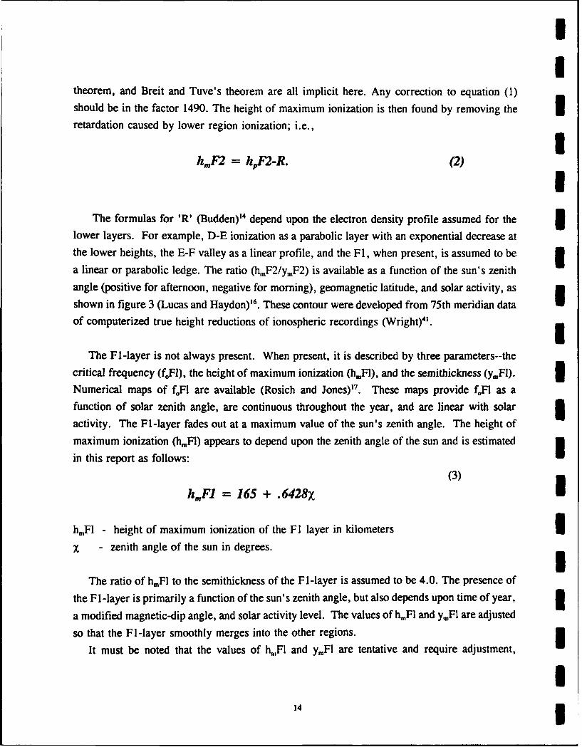
17.) Backscatter amplitudes and and ray-paths

RADARC is executed for a set of radar parameters, time of day, month of the year, some

specific azimuth, transmitter power, etc. and a predetermined maximum number of vertical

radiation angles, i.e. I to 45 degrees. It is run for each of these specific radiation angles. The

result describes a distribution of signal levels along the path for a one-way transmission. The

results of these one-way paths can then be inserted into the radar equation to determine the

received backscatter amplitude. A complete listing of the variables needed and the form they

should be in can be found in a discussion by Headrick°.

45

I

S• • I

Figure 12 Example raypaths of the backscatter signal

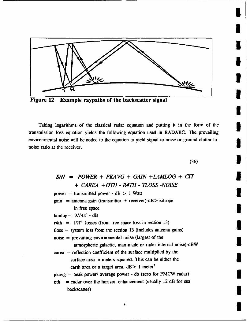
UTaking logarithms of the classical radar equation and putting it in the form of the

transmission loss equation yields the following equation used in RADARC. The prevailing

environmental noise will be added to the equation to yield signal-to-noise or ground clutter-to-

noise ratio at the receiver.

(36) 1S/N = POWER + PKAVG + GAIN +LAMLOG + CIT 5

+ CAREA +OTH - R4TH - MOSS -NOISE

power = transmitted power - dB > 1 Watt 3gain = antenna gain (transmitter + receiver)-dB > isitrope

in free space Ilamlog = XI/43 - dB

r4th = I/1W losses (from free space loss in section 13)

floss = system loss from the section 13 (includes antenna gains)

noise = prevailing envirnomental noise (largest of the

atmospheric galactic, man-made or radar internal noise)-dBW

carea = reflection coefficient of the surface multiplied by the

surface area in meters squared. This can be either the 5earth area or a target area. dB > 1 meter2

pkavg = peak power/ average power - db (zero for FMCW radar) 3oth = radar over the horizon enhancement (usually 12 dB for sea

backscatter) 34 1

cit = coherent integration time _ this is the time overwhich a returned waveform is summed at the receiver.

dB > 1 sec.

The OTH enhancement is a factor that accounts for multipath and the conductivity of thereflection area. A 6 dB figure seems more reasonable for an air target at altitude than the usual12 dB and is used by 12 ,") for surface targets.

The antenna gains must be in power gain for a signal level prediction. This means theefficiency must be known. To predict signal or ground clutter-to-noise the directive gain may beused.

The sections to follow will show in much detail what is needed for input informationto sucessfully execute the program RADARC and detailed output for executed sample input usingthe program.

18.) Summary

The mathematics associated with the ionospheric profile and ray-path generation arepresented for the OTH radar prediction routine RADARC-2. The method of calculating all lossesassociated with the computed ionosphere is illustrated in detail. The method of including the one-way losses into the radar equation for assessment of OTh radar is shown.

A complete internal description of all the modules formirg the Fortran code is included

for those wishing to make revisions or corrections to the computer code. The spread Dopplerclutter (SDC) code is included in this version of RADARC-2 and is easily invoked in the user

friendly input file. The computer program is complete and usable world-wide for OTH radarperformance calculations that include environmental noise and range dependent noise (SDC).

The Fortran code allows execution of the program on any machine using a floating pointnumber of at least 32 bits. Outputs can be chosen from many diverse printed tables or printer

graphics choices.

47

IIIIIIU

IPART IIi

* Users guide to RADARC input/output

I

Ia3I

UI

1.) Input

1.1) Files used by RADARCAll input to RADARC must be available before the program is executed. Several logical

assignments must be made as well. There is one input file which contains the run parametersfor the program; it is the only file that the user needs to prepare. There are up to sevennecessary data files; the exact number depends on the run parameters specified. One scratch fileis opened by the program, and it is deleted upon successful execution. These files are:

3 User preparedFORO 1 .DAT program control parameters (User specified)

3 Provided with RADARCCGMCS.BIN geomagnetic database used by CGMCSHFANTDIR:ANTXX optional antenna data fileHFDATDIR:GEOMAG.BIN geomagnetic database used by GEOMAGHFDATDIR:LANDMAP.BIN digitized map of major land massesHFDATDIR:MON.BIN monthly longterm ionospheric databaseHFDATDIR:MONNOISE.BIN monthly noise mapsHFDATDIR:YMCOEF.BIN maps of the ratio H./Y. for parabolic layers

I Created/destroyed by RADARCFOR099 scratch file created/deleted by RADARC

I The necessary logical assignments are:

FOROl I The user input file, if it has any name other than FORO11.dat oris not located in the default directory from which RADARC is run.

HFANTDIR The directory location of the antenna data files.HFDATDIR The directory location of all data files except those two specified

above.FOR010 A primary output file; assignment is optional.F0R032 A primary output file; assignment is optional.FOR034 A secondary output file; assignment is optional.

3 These assignments can be accomplished under Digital VMS with the followingstatements. The user must replace the term with the angle brackets with the3 appropriate specification; the brackets are omitted.

$ASSIGN <[userdirectory]user.input file> FOR011$ASSIGN <[antennadir]> HFANTDIR$ASSIGN <[antenna dir]> HFDATDIR$ASSIGN < [userdirectoryluser output fileI > FOR010

5

II

$ASSIGN <[userdirectoryluser output file_2> F0R032$ASSIGN <[userdirectory] user output file_3> F0R034 5

IIIU3IIIIII1I1I

52 3

UI

1.2) Details of user-specified run parameter file

The user-specified input file consists of a list of keywords, some with arguments. The

keywords are listed, one per line, with spaces delimiting keywords and arguments. Any line maybe made a comment by inserting an exclamation point (!). No portion of the line to the right ofthe exclamation point will be read; entire lines may be commented by putting the exclamationpoint in column 1. Neither blank lines nor lines without a recognizable keyword have any effect.The keywords and their associated arguments are described below, in alphabetical order. Asample input file follows.

I ANTTYPE Keyword to select the antenna. Takes 1 value. The value may be positiveor negative. If negative, its absolute value is used as the two-way gain.If positive, it is a built-in antenna type to be used in calculating the two-way gain. See the appropriate antenna routine (subroutine antXX). Theusages are mutually exclusive, and the last one input is used.

ex: anttype -50 ! Constant 2-way gain of 50 dB.anttype 12! Internal routine anti2 is used.

3 default: ANTTYPE -50

AZIMUTH This key allows the user to specify the 'look' azimuth of the radar, in

decimal degrees clockwise from geographic north. Takes 1 value.

default: AZIMUTH 77.

I CIT Specifies the coherent integration time, seconds. Takes a single value.

g default: CIT 1.0

ECLUT, IECLUT May also be IECLUT, either way it takes a single floating point argument,which is a multiplier for e clutter magnitude. Intended to reflect specificionospheric information only, and be left equal to 1 or 0 the rest of thetime.

I default: ECLUT 0.

EMULATE This keyword is a sort of meta-key: it takes no arguments and defines agroup of variables to be set in accordance with an earlier version ofradarc. The effect is immediate and overrides preceding keywords, butnot subsequent keywords.The variables affected, and their values after thiskey is used, are:

SCRPLT - SCRPLT status reverts to SNRPLT

* 53

II

CCRPLT - CCRPLT status reverts to CNRPLTLIMHOP 2 - only 2 hops are predicted 5AREAS 2 - 2 ionospheric sample areas are useSTEP 1400 - No sample is drawn at 0 distance;sample areas are at1400 and 2800.

default: inactive gFEC, HE, YMEFIC, HF1, YMF1F2C, HF2, YMF2 I

These parameters can be used to dictate a complete description of theregular layers of the ionosphere. Two values are associated with eachparameter. The first specifies the sample area to be associated with the Iinput value; the second is the input value itself. Defining the ionosphereat unused sample areas has no effect. Up to ten sample areas may bedefined.

FEC - E layer critical frequency.F1C - F1 layer critical frequency.F2C - F2 layer critical frequency.HE- Height of maximum ionization, E layer.HFI - Height of maximum ionization, F1 layer.HF2 - Height of maximum ionization, F2 layer.YME - Semithickness of a parabolic E layerYMF1- Semithickness of a parabolic F1 layerYMF2- Semithickness of a parabolic F2 layer

default: by default these parameters are calculated. 3FCLUT, IFCLUT May also be IFCLUT, either way it takes a real argument, which is a

multiplier for f clutter magnitude. It is intended to reflect specificionospheric information only, and be left equal to 1 or 0 the rest of thetime.

default: FCLUT 0.

FESL,FESM,FESU These parameters can be used to dictate the sporadic E layer. Two values 1are associated with each parameter. The first specifies the sample area tobe associated with the input value; the second is the input value itself.Defining the ionosphere at unused sample areas has no effect. Up to ten isample areas may be defined. Note that these parameters specify the Eslayer in a manner which differs from the regular modes. 3

FESL- Lower decile of Es critical frequency distribution.

5

CCRPLT - CCRPLT status reverts to CNRPLTLIMHOP 2 - only 2 hops are predictedAREAS 2 - 2 ionospheric sample areas are useSTEP 1400 - No sample is drawn at 0 distance;sample areas areat 1400 and 2800.

SHdefault: inactive

FEC, HE, YME

I FIC, HF1, YMF1F2C, HF2, YMF2

These parameters can be used to dictate a complete description of theregular layers of the ionosphere. Two values are associated with eachparameter. The first specifies the sample area to be associated with theinput value; the second is the input value itself. Defining the ionosphereat unused sample areas has no effect. Up to ten sample areas may bedefined.

FEC - E layer critical frequency.FIC - F1 layer critical frequency.F2C - F2 layer critical frequency.HE- Height of maximum ionization, E layer.HF1 - Height of maximum ionization, F1 layer.HF2 - Height of maximum ionization, F2 layer.YME - Semithickness of a parabolic E layerYMF1- Semithickness of a parabolic Fl layerYMF2- Semithickness of a parabolic F2 layer

I default: by default these parameters are calculated.

FCLUT, IFCLUT May also be IFCLUT, either way it takes a real argument, which is amultiplier for f clutter magnitude. It is intended to reflect specificionospheric information only, and be left equal to 1 or 0 the rest of thetime.

default: FCLUT 0.

I FESL,FESM,FESU These parameters can be used to dictate the sporadic E layer. Two valuesare associated with each parameter. The first specifies the sample area tobe associated with the input value; the second is the input value itself.Defining the ionosphere at unused sample areas has no effect. Up to tensample areas may be defined. Note that these parameters specify the Es3 layer in a manner which differs from the regular modes.

FESL- Lower decile of Es critical frequency distribution.

I

U

mFESM- median of Es critical frequency distribution.FESU- upper decile of Es critical frequency distribution. 5

default: by default these parameters are calculated.

FOE, FOFI, FOF2, FOESThese parameters are layer critical frequency multipliers, to be used tocustomize the program when specific data about the ionosphere is at hand. 1Generally, these should be set to 1, except for foEs which is set to .7.Each key takes a single value.

defaults: FOE1.,. FOFI 1.0. FOF2 1.0. FOES 0.7

FREQ, FREQMAX, FREQMIN, FREQSTEP 3The prediction may be run for a single frequency, using the 'freq'keyword, or a range of frequencies from 'freqmin' to 'freqmax' in'freqstep' MHz intervals. The two usages are mutually exclusive. Each Ukey takes 1 value.

default: FREQMIN 5.0. FREOMAX 28.0. FREOSTEP 1.0 1GROUND, SLANT An output option, these two parameters are mutually exclusive and only

the last will be used. The keyword takes no argument and specifieswhether slant or ground range will be used in the plots of CNR/SNR vs.range. I

default: GROUND

HOPS, HOPLIM, LIMHOP UThese keywords are synonyms. They designate how many hops out theprogram will calculate. The original radarc used 2 only. Now up to 4 areallowed. Takes 1 argument

default: LIMHOP 2

KFAC K factor is the local magnetic index used in ionospheric cluttercalculations. Takes I argument. 3default: KFAC 1.0

KP Kp is the planetary magnetic index, which is used in calculations ofionospheric clutter and in the calculation of the arctic oval. If this valueis negative the oval will not be calculated, but the absolute value will still 3be used for ionospheric clutter calculations.Takes 1 value.

5

UI

default: KP -3

I LSCAN Scan loss multiplier; takes 1 argument.

5default: LSCAN 0

MONTH Specifies the month to be predicted. Takes 1 value.

default: MONTH 1

I ORTHOAPT Aperture of the orthogonality effect; takes 1 argument. The aperture is thelargest deviation from orthogonality that produces clutter. The magnitudeof the clutter will be sin-function interpolated from zero at a deviationoutside ORTHOAPT to ORTHOMAG at orthogonality.

£ default: ORTHOAPT 0.0

ORTHOMAG Maximum value of orthogonality induced ionospheric clutter. Takes 1* argument.

default: ORTHOMAG 0.0

I PRINTOUT An output option taking 1 argument; the three values (1, 2, or 3) aremutually exclusive and only the last will be used. The output formats3 available, and the printout option that specifies them, are:

All printouts

fortran unit 10rayset tables up to limhop, regular modesrayset tables up to 2 hops, sporadic E modes

fortran unit 30vertical ionograms, by sample arearange coverage, amplitude vs time delay, by frequency (two-part

figure, if necessary)oblique ionograms ( 2 ionograms at different scales)combined raysets table

* printouts 2 and 3 only

fortran unit 323 range coverage part 1, amplitude vs time delay,by mode

angle coverage part 1, amplitude vs time delay,

31 57

II

by moderange coverage part 2 (if necessary), amplitude

vs time delay, by modeangle coverage part 2 (if necessary), amplitude

vs time delay, by mode 5printout 3 only

fortran unit 34echo internal values of inputmiscellaneous diagnostic information from ymap,lecden, fobby, I

setion, and setplt.

default: printout I ISYSLOS Specifies loss due to radar signal processing and other losses not

specifically included elswhere, dB.

default: SYSLOS 0.0

PULSEWIDTH Specifies pulsewidth to be used in the prediction, in microseconds. Takesa single value. This is required for earth backscatter area calculation.RADARC calculates SNR on an average power basis; therefore, signalbandwidth is not required.

default: PULSEWIDTH 120.0

SAMPLES, AREAS 1This optional parameter specifies the number of sample areas to use. the

keywords are synonymous. Take 1 argument. 5default: SAMPLES 10

SAMPLESTEP, AREA_STEP, STEPThese optional synonymous parameters specify the spacing betweensample areas. takes I argument.

default: 700 km

5I

UI

SITELAT The geographic north latitude of the transmitter in decimal degrees. Takestwo values: the first is numeric,the second is a single characternorth/south indicator. An 'S' will override the sign of the numeric valueand result in a point in the southern hemisphere. An 'N' or an omittedvalue will result in an interpretation from North. e.g. +north,-south.

ex: SITELAT -25. S yields 25 degrees southSITELAT 25. S yields 25 degrees southSITELAT 25. N yields 25 degrees northSITELAT -25. N yields 25 degrees southSITELAT 25. yields 25 degrees north

default: SITELAT 38.655 N

3 SITELONG The geographic west longitude of the transmitter in decimal degrees.Takes 2 values: the first is numeric, the second is a single characterEast/West indicator. The 'E' or 'W' characters are additive with the signof the numeric.

ex: SITELONG -77. W yields 77 degrees east5 SITELONG -77. E yields 77 degrees west

default: SITELONG 77.5 W

I SNRPLT, CNRPLT, SCRPLT, CCRPLTOutput options; the following options are, like many keywords in this list,mutually exclusive, and only the last will be used. The keywords take noarguments and specify:

SNRPLT - signal-to-noise ratio vs. range. This is the ratio of the signalassociated with the return from the target to the noise at thereceiver.5CNRPLT - clutter-to-noise ratio vs. range.This is the ratio of the signalassociated with the ground or sea return to the noise at thereceiver.

SCRPLT - signal-to-ionospheric clutter ratio vs. range. This is the ratioof the signal associated with the return from the target to thegreater of noise at the receiver or ionospheric clutter.

CCRPLT - clutter-to-ionospheric clutter ratio vs.range. This is the ratioof the signal associated with the ground or sea return to the greater3 of noise at the receiver or ionospheric clutter.

default: SNRPL

I SUNSPOT, FLUX Solar flux and sunspot are used for the same sorts of calculations. If eitheris input the program will calculate the other according to the relationship

9* 59

SI

below, to be used

FLUX = ((406.37+SUNSPOT)**2-93918.4)/1117.3 5SUNSPOT = SQRT(93918.4+1117.3*FLUX)-406.37

as called for; therefore only one of these is required. In fact, only one can Ibe used, because the last one input will cause the recalculation of previousflux/sunspot values. Each keyword takes a single value. 3default: SUNSPOT 70.

TARSIZE, TARTYPEThe radar target may be included as a fixed target size using 'TARSIZE',in dB above 1 sq. meter, or as a built-in target type, using 'TARTYPE'. ITartype and tarsize are mutually exclusive: the last one encountered willbe used. Each key requires 1 value.

default: TARSIZE 20

TIME, TIMESTART, TIMESTOP, TIMESKIP I24 hour GMT time at the transmitter for which a prediction is desired.Like the frequency, this parameter may be constant (use 'TIME'), ordefined as a loop from 'TIME-START' to 'TIME-STOP' by steps of'TIMESKIP'. Each key requires 1 value.

default: TIME 0. 1TXPOWER Allows specification of the transmitter power of the radar in kW. Takes 3

a single value.

default: TXPOWER 0.2 5WT The receive weighting factor; takes 1 argument.

default: WT 1.0

6III

II

XNOISE Receiver CCIR noise type if zero or negative, as given below,or noise indB below 1 watt if positive and not equal to 5. When equal to 5, thespecified noise is the greater of the natural noise and an approximate

i internal noise calculated in the program. Takes a single value.

CCIR man-made noise-1 Industrial-2 Residential-3 Rural-4 Remote

Internal noise options-5 use internal noise only (no natural noise)+5 manmade noise source is internal noise

default: +5

YEAR If the oval is turned off, this is cosmetic only, but with the oval turned onthis is necessary, and is used to figure solar epoch. Takes 1 value.

default: YEAR 1989

61

II

The following sample input file is a legal, unambiguous file, though messy.

! an ! indicates a comment or comment line! file: SAMPLE.INPsitelat 51.44 N ! latitude of transmitter decimal degree N+, S-sitelong 79.16 W ! longitude of transmitter W+, E-azimuth 275. ! 'look' azimuth deg CW from Northhops 2 ! calculate only 2 hops of predictions 3FREQMIN 5. ! you may select to run the prediction for a singleFREQMAX 28. ! frequency, using the "freq" keyword, or a range ofFREQSTEP 1 ! frequencies from "freqmin" to "freqmax" in "freqstep"U!FREQ 18. ! intervals, the two usages are mutually exclusive.txpower 200. ! KW)pulsewidth 120 ! Microseconds Icit 3.1 ! Coherent Integration Time, secondsxnoise -5 ! Receiver Noise type if negative, noise in dB below

1 watt if positive

antenna type may be positive or negative, if negative, it's absolutevalue is used as the two-way gain. If positive, it is an antenna type to be Iused in calculating the two-way gain. See the appropriate antennaroutine (subroutine antXX). The usages are mutually exclusive, and thelast one input is used.anttype -50 ! Constant gain antenna, 2-way gain = abs(-50)

anttype 12 ! Antenna type, last one controlsMONTH 6 ! Month Number (1 - 12)! GMT time at transmitterTIME 24 ! GMT time (1-24)!time start 2!timestop 3!time skip 1! if the oval is off, this is cosmetic only, but with the oval on this is! used to figure solar epoch.year 1991 ! Needed for arctic oval! solar flux and sunspot are used for the same sort of calculations. If flux! is input the program will calculate a sunspot number to use as called for.

Stherefore only one of these need be used in the deck. In fact only one can I! be used in the deck because the last one input will cause the recalculation! of previous flux/sunspot values.!flux 70 ! Can use either flux or sunspot number 3sunspot 100.! Kp is the planetary magnetic index, which is used in calculations! of ionospheric clutter and in the calculation of the arctic oval. If I!this value is negative the oval will not be calculated, but the absolute

6

I

value will still be used for ionospheric clutter calculations.I Kp 5 ! Magnetic activity (1-7) needed for arctic oval/trough

Kp -1.7 ! Negative value turns off oval, absolute value stillI used in Elkin's clutter algorithms, last one controls

! layer critical frequency multipliers, to be used to customize the program! when specific information about the ionosphere is known. Generally, these

should be set to 1, except for foEs which is set to .7I 1foE 1.0! foE multiplicative factor, default = 1.0foF1 1.0! foFl multiplicative factor, default = 1.0

I foF2 1.0 ! foF2 multiplicative factor, default = 1.0foEs .7 ! foes multiplicative factor, default = .70

tartype and tarsize are mutually exclusive, only the last one enteredI ! will be usedtartype -1 ! Target type, can use type or sizetarsize 17.0 ! Target size, dB above 1 sq. meter, last one controls! output options, the following three options are, like many inputs in! this list, mutually exclusive and only the last will be used.areas 2 ! this optional parameter specifies the number of sample areas to useareastep 1400. ! this optional parameter specifies the spacing between sample

areas.scrplt 1.0 ! Signal/max( ionospheric clutter, noise), last one controlssnrplt 1.0 ! Signal/noise plots, last one controlsccrplt 1.0 ! Clutter/noise plots, can use cnrplt or snrpltcnrplt 1.0 ! Signal/max( ionospheric clutter, noise), last one controlsI the argument is ignored

! output options, the following two options are mutually exclusive! and only the last will be used. The argument is ignored.ground 1.0 ! CNR or SNR plots vs range, last one controlsslant 1.0 ! CNR or SNR plots vs range, can use slant or ground! output options, the following three options are mutually exclusive! and only the last will be used.printout 1 ! Normal print out, last one controlsprintout 2 ! Individual frequencies printed out plus printout = 1!printout 3 ! Diagnostic print out plus printout = 2 and 1

WT 1.0 ! receive weighting factorKFAC 5 ! K factor is a local magnetic index used in ionospheric clutter

calculationsLSCAN 0 ! scan loss multiplierFCLUT 0.01 ! may also be IFCLUT, either way it is a real multiplier for f clutter

I1 63

magnitude. Should be used to reflect specific ionosphericinformation only, and be left equal to I or 0 the rest of the time.

ECLUT 0.01 ! may also be IECI-UT, either is a real multiplier for e cluttermagnitude. Should be used to reflect specific ionosphericinformation only, and be left equal to 1 or 0 the rest of the time.

ORTHOMAG .01 ! Maximum value of orthogonality induced ionospheric clutterORTHOAPT 0.1! Aperture of orthogonality effect;

largest deviation from orthogonality that produces clutter.

the ORTHO variables are left at .01 in this case because if they areset to zero, some calculations are never done. This is reasonableunless you want to see the magnetic aspect angle (labelled ORTHO degon the output), as we do lately.

This file is a legal, unambiguous input file just as it stands. Allmutually exclusive options are resolved by considering the lastinput only.

!EMULATE ! good idea to put this last to avoid accidental redefinition

64

UI

2.) Output

The output from RADARC consists of a number of tables and graphs spread over threefiles. The PRINTOUT keyword determines which output is produced. The files are on fortranunits 10, 32, and 34. These files will be named FOR010.DAT, FOR032.DAT, andFOR034.DAT, unless a logical assignment was made to reassign the unit before the programwas executed. These files will be referred to by their respective logical file names below.

2.1) FOR010: Single frequency rayset tables

I These tables show the basic geometry calculated by the program together with theassociated propagation characteristics. Each table has a heading which reports the basicrun parameters, and a body which reports the geometry and propagation characteristicsat each vertical take-off angle. The regular mode tables differ slightly from the sporadic-E mode tables. The items appearing in each table also vary with the run options

Sselected. Regular mode example rayset tables are presented in figures la,b. Sporadic-Emode example rayset tables are presented in figures 2a,b.

Values in the body of the tables are identified by abreviated column headings.3 These abreviations are described below:

SCOLUMN 1 This unlabelled column holds mode information. The mode symbols used in thisoutput are E, 1, 2, S, and +, representing the regular E, F,, F2,sporadic E, andover-the-MUFmodes, respectively. For example, 'E2' denotes a regular E modefollowed by an F2 mode.

ANG or the vertical take-off angle in degrees associated with the predicted raysetELANG geometry.

3 HITE the 'average' virtual height in kilometers for all hops.

TIME the total time delay in milliseconds for the ground range at the end of the last hop.

I GND the ground range in nautical miles to the end of the last hop.

SSLANT the (1-way) slant range in nautical miles to end of last hop.

C-AREA the radar cross section (RCS) of the sea/ground resolution cell at the end of the3 last propagation hop. This RCS is the product of the resolution cell area and thesurface scattering coefficient, oa. In this sample e = -29 dB.

T-AREA the size of the target in db relative to I square meter.

3 R4TH total two way free space loss to the end of the final hop.

* 65

I

tABS total non-deviative absorption.

DEV total deviative absorption.I

GNDLOS total ground reflection losses in db; omitted from 1 hop tables.

GT+GR combined transmit and receive antenna gain, in db.

CPINC the increment to ionospheric clutter power in db due to orthogonality of theraypath to the Earth's magnetic field. It is associated with the input key words:SCRPLT,CCRPLT, ORTHOAPT, ORTHOMAG. 'CPINC' only appears on 3the output when scrplt or ccrplt is selected, and its magnitude depends on orthoaptand orthomag.

ORTHO the angle between the raypath and the Earth's magnetic field at the target range.This column appears only when SCRPLT or CCRPLT is selected.

PROBE the predicted probability of ionospheric clutter originating in the E layer. Thiscolumn appears only when SCRPLT or CCRPLT is selected.

PROBF the predicted probability of ionospheric clutter originating in the F layer. Thiscolumn appears only when SCRPLT or CCRPLT is selected. 3

CPDB the total ionospheric clutter power resulting from the predictions of CPINC,PROBE, and PROBF. It is compared to other noise sources and the greatestbecomes the limiting noise for the prediction. This column appears only when ISCRPLT or CCRPLT is selected.

REF or total reflection losses on E, modes ILOSS

P-REC the predicted signal from the target, associated with T-AREA, in dbW.

CNR the ratio of the signal associated with C-AREA to the greatest noise source. (CNRand SNR differ by the same amount as C-AREA and T-AREA. I

SNR the ratio of the signal associated with T-AREA to the greatest noise source. (CNRand SNR differ by the same amount as C-AREA and T-AREA.

S the ionospheric sample area associated with the last hop. It is 'associated' because 3the properties of this sample area result in the most self-consistent predictiongeometry available. When the number of sample areas is limited, the sample areachosen may not result in a perfectly self-consistent prediction. For example, 3imagine the program is calculating the characteristics of the second hop of a two-

6

IU

hop prediction. The characteristics of the first hop are known. Let us say thesecond hop begins at a ground distance of 5000 nm. The properties of the samplearea located at 2500 nm suggest that the reflection area for the second hop shouldbe around 7500 nm (geometry just like the first hop). So the program performsa calculation for the sample area located nearest 7500 nm, but the properties ofthat sample area suggest that the true reflection area may be nearer 9000 nm. Ifno other sample is available, then the program must use the sample at 7500 nm3 and a small inconsistency must be tolerated. Were other samples available theprogram would attempt to home on the best one. In practice this effect is smallunless the ionosphere is changing rapidly between sample areas.

II

III

III

I

II

CM 30P RAY 33! YABLE OUR 221100 TJJ34324 UT FRXOOMWCY- 13.000 W3 17-DEC-1992 11.34 5YU8113341TU.tA 51.49 LAT -79.23 LOW A3TTM? 12

3Iuutl.275.?.o DIrG BIANIDE. 0.43 D03 NI03•3-175.54 DOWPRAUK -fts 3.0 DOW1 LA3630A 80/4P1 COMR. -5.7 D03N AURORAU LOSS. 4.5 DRAVGlfll DU10 0.0 D5. 03M •nCIURMO . 6.0 DR INT. TINE. 3.10 SiC (OR 4.9 DR)

LOSS COLtNS) is m OF AV)30tAL. ADSE, DEVI OBF LOSSS•CEI(DB) 12 5314 AS 503(D0) ELOV 3ZCREP3 C-ARRA(BACK3CARIEP ARIA) 1S USED 10 TARGE? SIZZ513(D3)PEUX MR + GT.QR 0 LAMBDA 3Q/4P1 CODE - R4TH - LOSS - NO1 . TARCUT SIZE

SAVrAOE/P3AZ MR RATIO * OTE PAT1 MEARCUIM0T 4 INETEGRATION TI3ALL 3EPRESS3ODO D0 FOR A OUR 331TZ BAMDMIDT

TIMM •LM30 RITZ 0 SLANT 01.0R C-AR•A T-AREA R4T8 ABS DEV OF L6OSS P-REC CIR M3R

NSE D3 109 Em N• s D0381 D0811 D3N DR D3 D3 DB D0W D0 D33 10.12 0.0 113.4 1289. 1302. 0.0 57.8 17.0 255.3 19.7 3.5 0.0 29.7 -149.0 4.5 -34.3 2

I 14.72 1.0 113.8 1173. 1189. 15.3 57.4 17.0 253.7 19.6 3.5 0.9 29.7 -152.0 23.5 -13.9 2a 13.49 2.0 114.5 1076. 1090. 31.5 S7.0 17.0 252.2 19.4 3.4 0.0 29.5 -134.9 40.4 0.0 2

R 12.43 5.0 115.8 990. 1004. 37.1 S6.7 17.0 250.8 18.9 3.8 0.0 29.2 -128.0 47.5 7.9 29 11.52 4.0 117.3 916. 931. 42.8 51.3 17.0 249.5 18.4 4.0 0.0 28.9 -2121.0 54.4 05.2

3 10.75 5.0 120.0 353. 308. 45.5 54.1 17.0 248.3 17.7 4.3 0.0 28.5 -117.1 53.5 19.4 2

3 10.41 6.0 128.0 823. 841. 43.1 55.9 17.0 247.7 17.0 5.1 0.0 28.6 -114.1 41.5 22.5 21 14.83 7.0 273.5 1307. 1342. 49.1 53.0 17.0 254.1 14.3 10.0 10.4 43.4 -134.2 41.4 0.3 2

1 14.03 8.0 274.6 1233. 1295. 50.0 57.8 17.0 255.2 15.5 V.0 f.4 40.4 -129.8 45.3 5.0 2 I1 15.41 9.0 279.3 1134. 1245. 51.0 57.7 17.0 254.5 14.8 7.5 8.5 37.3 -125.0 s0.5 9.9 21 15.03 10.0 238.6 1152. 1215. 52.0 57.4 17.0 254.1 14.1 7.4 7.5 35.5 -121.9 53.7 13.1 2

1 15.35 11.0 315.7 1108. 1240. 52.2 57.7 17.0 254.4 13.5 9.7 6.5 36.2 -122.4 53.0 12.3 2

2 18.02 12.0 410.9 1349. 1454. 52.5 58.4 17.0 257.2 12.8 7.8 5.4 32.7 -120.9 S4.7 13.3 2

2 14.59 13.0 389.1 1239. 1340. 52.5 53.0 17.0 255.8 12.2 4.6 4.8 28.1 -115.2 60.3 19.3 22 XS.$8 14.0 378.3 1100. 1250. $2.5 57.8 17.0 254.7 11.7 0.3 4.0 24.5 -112.8 02.8 22.0 22 14.80 15.0 372.9 1098. 1194. 52.0 57.6 17.0 253.8 11.2 3.4 3.3 24.4 -110.5 05.0 24.4 2

2 14.21 14.0 371.8 1049. 2148. 51.4 57.4 17.0 253.1 10.7 3.4 2.7 23.3 -109.3 04.2 25.3 22 13.73 17.0 373.2 1008. 1110. 50.7 57.3 17.0 252.5 10.3 3.3 2.2 22.2 -108.4 07.0 26.7 22 13.37 18.0 377.2 975. 1080. 49.9 57.2 17.0 252.0 9.8 3.4 1.8 21.5 -108.2 07.3 27.1 22 13.12 19.0 384.4 950. 2050. 49.2 S7.1 17.0 251.7 9.5 3.0 2.0 22.0 -208.1 07.4 27.3 2

2 12.93 20.0 393.2 932. 1045. 48.4 57.1 17.0 251.S 9.1 3.9 1.1 20.4 -108.2 47.3 27.2 2

2 12.39 21.0 404.4 918. 1041. 48.0 57.1 17.0 251.4 8.8 4.5 0.9 30.4 -103.7 44.9 24.8 2

2 12.97 22.0 424.3 915. 1043. 47.4 57.2 17.0 251.5 8.5 5.1 0.4 20.7 -109.4 44.1 25.9 22 13.25 23.0 449.4 935. 1070. 44.9 57.3 17.0 251.9 8.2 4.3 0.5 21.5 -110.9 44., 24.3 22 13.95 24.0 492.1 941. 1127. 44.4 57.9 27.9 353.8 7.9 8.4 0.4 33.2 -113.7 41.8 21.2 22 17.43 2S.0 4S2.4 1145. 1403. 44.2 58.4 17.0 254.7 7.7 19.3 0.3 33.7 -127.4 48.2 4.4 2* I.SS 24.0 424.3 790. 933. 45.9 54.8 17.0 249.5 7.4 27.3 0.0 41.7 -130.2 45.3 5.5 2

* 11.25 27.0 424.3 742. 909. 45.3 54.7 17.0 249.0 7.2 37.2 0.0 50.9 -139.1 34.4 -3.3 2* 10.94 28.0 424.3 735. M35. 45.7 54.7 17.0 248.4 7.0 47.0 0.0 01.3 -149.2 26.3 -13.4 2

* 10.68 29.0 424.3 710. 343. 45.4 54.6 17.0 245.1 4.8 59.1 0.0 72.4 -1,0.3 15.2 -24. 24* 10.42 30.0 424.3 430. 842. 45.0 54.5 17.0 247.7 4.4 70.4 0.0 33.7 -171.7 3.9 -35.7 2

* 10.18 31.0 424.3 443. 322. 44.3 54.5 17.0 247.3 4.4 82.0 0.0 95.0 -133.3 -7.7 -47.2 2

* 9.94 32.0 424.3 641. 303. 63.0 54.4 17.0 240.9 4.3 93.1 0.0 105.9 -194.5 -19.0 -58.4 2* 9.72 33.0 424.3 019. 785. 42.3 50.4 17.0 246.5 0.1 103.7 0.0 114.3 -205.5 -30.0 -09.3 2

* 9.51 34.0 424.3 599. 748. 41.9 54.3 17.0 244.1 0.0 103.8 0.0 110.3 -206.0 -30.4 -49.7 2* 9.31 35.0 424.3 579. 752. 41.3 54.3 17.0 245.3 5.3 103.3 0.0 114.1 -20o.1 -30.4 -49.9 2* 9.12 34.0 424.3 500. 737. 40.0 50.2 17.0 245.4 5.7 103.3 0.0 116.0 -206.3 -30.8 -70.0 2

8 3.94 37.0 424.3 542. 722. 40.3 54.2 17.0 245.1 5.6 103.8 0.0 115.9 -200.2 -30.7 -49.9 2* 0.77 38.0 424.3 525. 700. 40.0 54.2 17.0 244.7 5.5 103.3 0.0 115.8 -204.1 -30.5 -49.7 2

* .40 39.0 424.3 503. 495. 39.5 56.2 17.0 244.4 5.4 103.3 0.0 115.7 -204.2 -30.4 -09.3 2

38.45 40.0 424.3 49, g33. 39.0 54.2 17.0 244.1 5.3 103.8 0.0 115.4 -204.2 -30.7 -49.8 2

38.30 41.0 424.3 474. 471. 37.2 56.1 17.0 243.3 5.2 103.8 0.0 115.5 -207.7 -32.2 -71.3 2S 8.10 42.0 424.3 460. 45t. 55.3 50.1 17.0 243.5 5.1 103.8 0.0 115.4 -209.2 -33.7 -72.8 2

* 3.02 43.0 434.3 444. 043. 33.7 5#.1 17.0 243.2 5.0 103.8 0.0 115.3 -210.4 -34.9 -74. .023

* 7.89 44.0 42d.3 431. 433. 32.2 50.1 17.0 242.9 4.9 103.3 0.0 115.2 -211.0 -30.1 -75.2 2

FIGURE la: Example regular mode rayset table. (one hop) I

!I

I

II

TWO 3OP RAT 33T TABLE .2M 38101.00 TYIM.24 OT FREQUEICY. 13.000 NNZ 17-DWC-1299 11s36035UR31TT6s S1.49 LAY -79.23 LU ATTYP 12IJMIM.27S.00 DSa zrANNTMr . 0.63 DUG NOZEU-175.54 DONMA IRA. 53.0 D01 LANSDA BQiPI• CUZl. -5.7 DRiS AORAL LOSS. 6.5 USAVG/PW 5113, 0.0 ON. OTS I0RACDERPUT•, S.0 DR IN?. Trll•: 3.10 SEC fOR 4.9 DO)

L wg os OU 1;1 SU Op AVOIA, AS$,, Zs. ow. GXDLOS ,if82CM(DO) 18 AM A 9M1(M0) DmA. EXCEPT C-AJrA(ACRNCAY1UT AREA) 12 USED 'On TARGEN SIZSUIDW)•.SAPIER * 0+GR + O IADA 5/4PI CUSD - 0TI- 038-LOSS - 10I29 * TARGET SCZE

* &VIUtGZIPlUU PWi RAIYO 4 OTSl PATH IMRAMMUNM * INTEGRATION flimALL EXriSILuDIN DR FOR A 062 RENtTZ XMIJU_2•TIm ? Ru RITZ 000 3LAI1 GT.GX C-ANIA T-A]MA 44TR ADS DiN OBP GwDOS LOSS P-IUC m mom

NumC no 03 m w U s3 D03 0N303 DARK DUN DO DR DU Da DR Dim Do DO

ZN 31.94 0.0 111.5 2555. 2580. 0.0 60.8 17.0 267.2 46.6 6.0 0.0 12.0 71.0 -219.2 -43.7 -87.4ME 29.14 1.0 111.7 23238. 2354. 15.8 60.4 17.0 265.6 46.3 6.0 0.0 0.8 59.7 -101.0 -15.4 -S3.8U 24.66 2:. 112.2 2127. 2154. 31.5 60.0 17.0 264.0 45.7 6.2 0.0 3.2 61.6 -175.9 -0.4 -43.3

24 .50 3.0 113.3 19S2. 1960. 37.1 5t.$ 17.0 202.6 44.7 6.4 0.0 2.4 40.1 -167.7 7.0 -34.8OR 22.65 4.0 114.7 1801. 1230. 42.8 59.3 17.0 261.2 43.3 7.1 0.0 1.9 58.8 -159.7 15.8 -26.4ME 21.07 S.0 116.6 1673. 1703. 45.S S9.0 17.0 320.0 41.8 7.6 0.0 1.5 57.S -154.0 20.6 -21.2

uN 20.06 6.0 121.8 1538. 1431. 48.1 56.8 17.0 250.1 40.1 8.7 0.0 1.3 56.7 -150.7 24.9 -16.91N 25.55 7.0 1:5., 2024. 2056. 40.1 55.: 17.0 263.1 38.: 13.: 10.6 1.2 70.: -167.0 8.5 -34.4aN 24:.6 0.0 150.2 1015. 1553. 50.0 55.7 17.0 262.7 36.7 13.5 0.6 1.0 67.3 -162.1 13.4 -21.21N 24.10 9.0 204.5 1367. 1147. 51.0 S5.6 17.0 262.3 35.0 12.4 8.5 6.6 Go.5 -162.4 13.1 -29.S11 20.24 10.0 266.4 2165. 2282. 52.0 60.3 17.0 265.0 33.3 19.7 16.3 7.2 83.0 -177.6 -2.0 -45.311 27.86 11.0 279.5 2128. 2251. 52.2 60.3 17.0 264.8 31.7 15.0 14.0 7.8 75.0 -173.1 2.4 -40.021 30.07 12.0 328.5 2270. 2425. 52.5 60.6 17.0 266.1 30.3 16.6 11.8 0.7 66.1 -160.9 14.6 -29.021 3.35 13.0 321.7 2134. 2251. 52.5 60.4 17.0 265.1 28.5 12.59 5. 0.7 56.7 -152.6 22.7 -20.621 27.44 14.6 324.9 2057. 2217. 52.5 60.2 17.0 264.5 27.6 13.2 3.1 5.4 64.8 -15.4 17.1 -26.12 31.41 15.0 402.4 2326. 2564. 53.0 60.5 17.0 266.5 26.4 9.6 6.6 9.9 59.2 -15S.1 20.5 -23.422 25.72 16.0 392.4 2187. 2401. 51.4 60.6 17.6 265.5 25.2 9.6 5.3 0.6 47.1 -142.8 32.7 -10.522 238.42 17.0 338.7 2081. 2297. 50.7 60.5 17.0 265.1 24.2 3.7 4.2 0.5 44.1 -135.9 35.7 -7.322 27.50 10.0 35.:9 2002. 2222. 45.5 60.3 17.0 244.6 23.2 3.7 3.2 0.5 42.2 -138.3 37.2 -1.12226.33 1:.0 354.5 1040. 2167. 40.2 60.3 17.0 264.1 22.3 3.6 2.5 0.5 40.6 -137.1 38.5 -422 26.36 20.0 401.8 1802. 2130. 48.6 60.2 17.0 263.8 21.5 0.4 1.5 0.5 31.7 -136.6 39.0 -4.222 26.14 21.0 413.0 1861. 212. 48.0 60.2 17.0 263.7 20.7 10.3 1.4 0.5 39.3 -136.6 38.5 -4.322 26.24 22.0 429.8 1850. 2120. 47.4 60.2 17.0 263.8 20.0 11.5 1.0 0.4 39.5 -137.3 38.2 -5.0

22 26.67 23.0 452.8 18361. 215S. 46.5 60.3 17.0 264.0 10.3 13.6 0.7 0.4 40.6 -131.1 36.4 -6.922 27.75 24.0 450.0 1914. 2246. 46.4 40.6 17.0 264.3 13.7 17.2 0.S 0.4 43.3 -142.6 32.7 -10.522 32. 4 25.0 602.3 3105. 2425. 46.2 61.3 17.0 267.5 10.1 31.6 0.4 13.8 70.6 -172.4 3.2 -41.1I23.38 36.0 435.8 15P7. A10S. 45.5 S5.• 17.0 261.8 17.5 56.4 0.0 0.4 0.6 -173.S -3.8 -4S.9

22.76 37.6 420.8 1541. 1839. 45.8 50.8 17.0 261.3 17.0 75.0 0.0 0.4 50.0 -196.3 -20.l -43.4.. 22.17 26.0 420.0 1467. 1702. 45.7 5.7 17.0 260.0 14.5 56.0 0.0 14.6 133.6 -236.6 -SS.2 -56.0. 21.62 25.0 421.0 1436. 1747. 4S.4 55.7 17.0 260.4 16.0 110.4 0.0 14.8 155.0 -253.0 -77.4 -126.1.. 21.05 30.6 4:2.6 1307. 17 45.017.6 260.6 141.4 0.0 15.1 178.S -275.7 -10.1 -143.7

20.66 31.0 420.0 1341. 164.43 4.3 5s.5 17.0 255.6 15.2 164.1 0.0 15.3 201.1 -258.4 -123.0 -135.•20.12 32.0 430.6 1206. 1426. 43.6 55.5 17.0 250.2 14.0 1•6.2 0.6 15.5 223.0 -320.5 -145.3 -187.8IS: 15.i3 33.0 420.0 1253. 1550. 42.3 59.4 17.0 250.6 14.5 207.4 0.0 15.7 244.0 -342.4 -16•.0 -205.3

.. 10.25 34.0 432.0 1212. 1556. 41.0 55.4 17.0 258.4 14.1 208.0 0.6 15.5 245.3 -344.2 -168.7 -211.1*. 18.85 35.0 425.8 1172. 1523. 41.3 5$.3 17.0 258.0 13.8 2080. 0.0 16.0 245.2 -366.3 -1638. -211.2,108.46 34.0 429.• 1134. 1412. 40.6 50.3 17.0 257.7 13.5 208.0 0.0 16.2 245.0 -344.5 -145.0 -211.3

10.10 37.0 420.8 1017. 1462. 40.3 59.3 17.0 257.3 13.2 208.5 0.0 16.3 244.9 -346.4 -146.9 -211.117.75 36.0 420•. 1042. 1434. 40.0 55.3 17.0 257.0 12.0 208.5 0.0 16.5 244.8 -344.3 -160.7 -211.0

.. 17.42 3:.0 425.: 1027. 1406. 35.5 35.2 17.0 256.6 12.7 208.t 0.0 16.6 244.• -344.3 -146.8 -211.017.11 40.3 420.0 554. 1382. 30.0 50.2 17.0 256.3 12.4 200.5 0.0 16.7 244.5 -344.4 -126.8 -211.0

*. 160 41. 8 4 125 62. 1358. 37.2 50.2 17.0 256.0 12.2 2086. 0.0 16.8 244.4 -345.6 -170.3 -212.S

*. 16.52 42.0 420.8 931. 1335. 35.3 55.2 17.0 255.7 12.0 208.9 0.0 14.0 344.3 -347.3 -171.3 -213.5.4 16.25 43.8 425.8 501. 1313. 33.7 50.2 17.0 255.4 11.8 208.0 0.0 17.0 244.1 -348.4 -172.5 -215.144 15.08 44.0 462.6 872. 1212. 32.2 50.2 17.0 255.2 11.6 208.9 0.0 17.1 244.0 -345.6 -174.1 -216.3

I FIGURE Ib: Example regular mode rayset table. (two hop)

II

II

ONE 3O0 RAT SIT TABLE JUN SESMl00 TIIM-24 UT FREQUENCY- 13.000 MZ 17-DEC-1992 11.36

TRAHXNEMTTZX S1.410 LA? -79.22 LONG RMTP 12 IEEAIJ00G . 275.00 DEt BJANNIDTR . 0.03 D3G NOISE . -175.54 DOWPrAK EWR 53.0 DOW LIIDD BQ/4P1 COE - -5.7 DISN&VG/fl PWR - 0.0 DS. O91 M3ANCRaMc T . 6.0 DB liT. TIME - 3.10 23C (OR 4.9 DR)

LOSS COLUMI is EQUAL TO 331 LOSSC0R13D) 1 SAME AS Sm(DB) RBELOW EXCEPT C-ARAA(BACKICATTER AMrA) 19 USED FOR TARGET 3233r,INR(UD) - PEAK WR . GT+R * LAMBDA 30104P CUDED - R•42 - LOSS - NOISE + TARGET SIZE

4 AVEAGE/PEAU PW RATIO . 091 PATE IlNAmCRmfhT . INTEGRATION TINEALL EXPRESSED IN DS FOR A NE 3n'TZ DANMIDOTE

TINE ZLA" DITE OND SLANT 0T9.R C-ARIA T-ARZA R4TH RE1 LOSE P-REC C0U SHENSEC D3G IN NN JI D DRMN DEIN DM 03 DB DBEWl 0 D 3 DB

5 15.806 0.0 110.0 1229. 1281. 0.0 57.7 17.0 255.0 39.1 39.1 -183.1 -2.7 -43.4

8 14.45 1.0 110.0 1155. 1147. 15.8 57.3 17.0 253.4 39.2 39.2 -166.2 14.2 -20.1a 13.17 2.0 110.0 1051. 104. 31.5 50.9 17.0 251.8 39.4 39.4 -149.5 31.0 -8.91 12.02 3.0 110.0 959. 972. 37.1 56.5 17.0 250.2 39.9 39.9 -143.1 37.4 -2.22 11.00 4.0 110.0 670. 859. 42.6 50.2 17.0 245.7 40.6 40.0 -137.2 43.2 4.1a 10.10 S.0 110.0 602. 614. 45.S 55.6 17.0 247.2 42.4 42.4 -135.1 45.4 0.0a 0.30 0.0 110.0 737. 751. 48.1 55.4 17.0 245.7 44.2 44.2 -133.1 47.3 8.99 0.59 7.0 110.0 079. 094. 49.1 55.1 17.0 244.4 44.9 44.9 -131.8 48.7 10.0a 7.90 8.0 110.0 628. 643. 50.0 54.8 17.0 243.0 45.9 45.9 -130.9 49.0 11.88 7.40 9.0 110.0 582. 596. 51.0 54.5 17.0 241.5 47.2 47.2 -130.3 50.2 12.7a 0.91 10.0 110.0 542. 558. 52.0 54.2 17.0 240.4 49.1 49.1 -130.2 50.2 13.12 0.47 11.0 110.0 506. 523. 52.2 53.9 17.0 239.4 51.5 51.5 -131.5 48.9 12.03 0.06 12.0 110.0 073. 491. 52.5 53.7 17.0 236.3 54.0 54. -133.S 40.9 10.33 5.72 13.0 110.0 444. 402. 52.5 53.4 17.0 237.3 58.5 58.5 -136.7 43.8 7.41 5.41 14.0 110.0 416. 437. 52.5 53.2 17.0 236.3 03.5 63.5 -140.9 39.0 3.49 5.12 15.0 110.0 394. 414. 52.0 53.0 17.0 23,.4 09.0 49.0 -1406.8 33.0 -2.3 I

4 •.87 10.0 110.0 372. 393. 51.4 52.6 17 " 77.3 77.3 -154.3 20.1 -9.04 4.43 17.0 110.0 353. 374. 50.7 52.0 17.0 233.0 86.9 80.9 -144.0 10.4 -19.1

3 4.42 16.0 110.0 334. 357. 49.9 52.4 17.0 232.8 98.9 98.9 -176.1 4.3 -31.15 4.22 19.0 110.0 318. 341. 49.2 52.2 17.0 232.0 113.9 113.9 -191.2 -10.7 -45.9a 4.05 20.0 110.0 303. 327. 48.6 52.1 17.0 231.3 132.7 132.7 -210.1 -29.0 -04.72 3.86 21.0 110.0 2859. 314. 48.0 51.9 17.0 230.4 156.5 150.5 -233.8 -53.4 -80.38 3.73 22.0 110.0 275. 302. 47.4 51.8 17.0 229.9 186.6 1860. -203.9 -03.5 -118.3a 3.59 23.0 110.0 263. 290. 40.9 51.0 17.0 229.2 225.0 22S.0 -302.3 -121.9 -150.53 3.47 24.0 110.0 252. 200. 40.4 51.5 17.0 228.0 274.3 274.2 -351.5 -171.1 -205.0a 3.35 25.0 116.0 241. 270. 40.2 51.4 17.0 220.0 337.7 337.7 -414.0 -234.4 -248.83 3.24 26.0 110.0 331. 241. 45.9 51.3 17.0 227.4 420.2 420.2 -497.1 -310.6 -350.9S 3.13 27.0 110.0 322. 253. 45.8 51.2 17.0 220.0 452.8 452.8 -529.3 -348.9 -383.1• 3.04 28.0 110.0 313. 245. 45.7 51.1 17.0 226.3 452.4 452.4 -528.0 -348.3 -362.4

I 2.95 29.0 110.0 205. 2311. 45.4 51.0 17.0 225.0 452.4 452.4 -528.5 -348.1 -382.18 2.04 30.0 110.0 107. 231. 45.0 50.9 17.0 225.3 452.2 452.2 -528.3 -347.6 -381.7a 2.79 31.0 110.0 190. 235. 44.3 50.0 17.0 224.0 452.0 4532.0 -528.4 -347.9 -381.8

2 2.71 32.0 110.0 183. 219. 43.0 50.6 17.0 224.3 451.9 451.9 -528.5 -348.1 -301.0a 2.44 33.0 110.0 176. 214. 42.0 50.7 17.0 223.9 451.7 451.7 -520.3 -348.4 -382.19 2.58 34.0 110.0 170. 208. 41.9 50.7 17.0 223.4 451.0 451.0 -529.2 -348.7 -382.48 2.52 35.0 110.0 104. 203. 41.3 50.6 17.0 223.0 451.4 451.4 -529.3 -346.8 -382.4a 2.46 30.0 110.0 150. 199. 40.6 50.4 17.0 223.0 451.3 451.3 -52t.5 -349.0 -362.02 2.40 37.0 110.0 153. 194. 40.3 50.5 17.0 222.2 451.2 451.2 -529.3 -348.8 -302.4

2 2.35 36.0 110.0 147. 190. 40.0 50.5 17.0 221.9 451.1 451.1 -529.2 -348.7 -382.2• 2.30 39.0 110.0 142. 100. 30.5 50.4 17.0 221.5 451.0 451.0 -529.2 -348.7 -302.28 2.24 40.0 110.0 138. 182. 39.0 50.4 17.0 221.1 450.9 450.9 -529.3 -340.8 -382.23 2.21 41.0 110.0 133. 179. 37.2 50.4 17.0 220.8 450.8 450.8 -530.7 -350.3 -383.70 2.17 42.0 110.0 128. 175. 35.3 50.4 17.0 220.5 450.7 450.7 -532.2 -351.7 -385.1a 2.13 43.0 110.0 124. 172. 33.7 50.4 17.0 220.1 450.0 450.4 -533.3 -352.9 -380.3 II 2.09 44.0 110.0 120. 149. 32.2 50.4 17.0 219.8 4S0.5 450.5 -534.5 -354.1 -307.4

FIGURE 2a: Example _poradic-E mode rayset table. (one hop) I

III

'° U

IU

T OP N AY RTS TANS O7W 811.100 •¶•M324 UT VR•R 1CY= 13.000 On2 17-D&C-1992 11.36TRAMITTOZA. 51.43 LA? -79.23 LONG ANM? 12ZREAING - 275.00 UO U•UAWMIDYU - 0.63 DIG NOUR . -175.54 DUNPlau M. * 53.0 DUW LAREDA 3Q/4P1 CORE - -5.7 DORBAVG/PU PRO . 0.0 DR. OTI RAJICIYN - 6.0 DR INT. TZKZ - 3.10 SIC (0 4.9 DR)

LOSS COLwUl is 8U91 o0 ORP Am SDLOS WOSESRJUlDS) 18 SM AS MSR(DR) BDEOW EXCEPT C-MAREA (CMECATNIt ARIA) 1U OgnD FOR ARGET SIZEIrtS) - L O + GT+QA - N SO/0P1 C - R4ODO - LOSS - 01 * SThGT SZE

+ AVRIGIUU AK / PIM ql RATIO . OTR PAU• INiUMMONT * INTEGRATION TZ]ALL nm~u•saD in Do IFOR A cam RunS aJmmiDS•H

TIM KUM NZS'R WD SLANrT GT*GR C -AR]UA T -JLPJ ROTR RIFP =DLIOS LOSS P-R.JC cm SHR

KR DG O N m - DB Do= DUNN DUN D9 DR DR DOW DR DR88 31.72 0.0 110.0 2358. 2563. 0.0 60.7 17.0 247.1 44.1 12.0 95.2 -248.2 067.0 -111.529 26.05 1.0 110.0 2359. 2334. 15.8 00.3 17.0 205.4 44.0 0.6844.1 -220.1 -33.7 -63.0

2. 34 3.2 110.0 2102. 2128. 31:5 17: 27. ,303.9 . 1.7 34.9 -204.0 -23.6 -33.588 3i. OS 3.0 110.0 1917. 1933. 37.1 59.5 17.0 202.2 33.7 2.4 33.0-150.2 -17.3 -30.3£9 22.01 4.0 110.0 1752. 1778. 42.8 59.2 17.0 230.7 43.6 3.2 87.5 -193.0 -12.3 -53.735 20.20 5.0 110.0 1004. 1632. 45.5 58.8 17.0 259.2 43.7 3.9 90.1 -191.7 -11.3 -53.1

18 3.0 110.0 1474. 1502. 48.1 58.4 17.0 257.8 34.3 4.6 93.2 -191.1 -10.7 -52.133 17.17 7.0 110.0 1358. 1388. 49.1 53.1 17.0 253.4 45.8 5.3 93.0 -1M1.9 -11.4 -52.6

1:: 15.23:.0 110.0 1253. 1233. 50.0 57.3 .0 0 255.1 33.23 .0 100.0 -193.0 -13.5 -53.33I 13.30 9.0 110.0 1305. 1193. 51.0 57.5 17.0 253.0 49.3 3.1 103.1 -175.2 -13.7 -55.2

22 13.02 10.0 110.0 1085. 1113. 52.0 57.2 17.0 252.0 50.5 7.2 107.2 -197.4 -13.9 -57.138 12.14 11.0 110.0 1011. 1045. 52.2 56.9 17.0 251.5 53.3 7.3 112.3 -201.0 -21.2 -31.158 12.15 12.0 110.0 943. 932. 52.5 53.7 17.0 250.3 53.3 0.3 119.5 -207.5 -27.0 -33.7

35 11.53 1. 2. 5. •4 25 5. 70 3•4 0 . 3. 300 -501•5 13.0 110.0 000. 925. 52.5 53.3 17.0 239.3 31.0 0.9 120.4 -215.5 -35.1 -73.538 10.02 13.0 110.0 535. 073. 52.5 53.2 17.0 250.3 53.3 8.3 139.3 -223.0 -35.0 -03.7:: 10.25 15.0 110.0 703. 023. 52.0 $5.0 17.0 247.4 7 :. : 1.9 153.9 -230.1 -59.7 -90.7

9 5.73 14.0 110.0 745. 780. 51.4 55.3 17.0 243.5 04.5 10.4 172.2 -258.2 -77.7 -110.5SO 9.23 17.0 110.0 705. 748. 50.7 55.3 17.0 245.7 97.7 10.8 195.4 -2381.5 -101.1 -131.7II 3.34 13.0 110.0 039. 713. 39.9 55.4 17.0 2344.9 115.2 11.2 225.3 -311.0 -131.1 -109.53s 0.45 19.0 110.0 333. 731. 39.2 55.2 17.0 243.1 135.3 11.7 233.3 -350.3 -103.0 -200.0

08 .09 20.0 110.0 305. 054. 33.3 55.1 17.0 233.3 139.3 12.0 313.3 -300.7 -220.2 -253. 35: 7.77 21.0 110.0 577. 432. 40.0 53.9 17.0 242.3 211.3 12.3 300.5 -333.9 -233.4 -32.4•3• 7.47 22.0 110.0 551. 303. 47.4 53.0 17.0 231.9 239.0 12.3 433.4 -553.3 -374.4 -312.122 7.19 23.0 110.0 527. 501. 43.9 54.7 17.0 241.3 330.2 13.1 533.3 -372.7 -392.2 -529.9

05 7.93 24.0 110.0 504. 503. 47.4 54.5 17.0 240.3 254. 123.3 743.0 -330.3 -374.4 -317.529 0.9 235.0 110.0 532. 531. 43.2 54.7 17.0 230.0 353.0 13.0 307.5 -0932. -713.2 -750.3

38 0.47 24.0 110.0 4 33. 5 3. 45.9 5 3.3 17.0 23 3.4 4 95.7 14.3 07 9.0 -8750. -7 5. * -6332.7

3 .27 27.0 110.0 333. 503. 35.3• 54.2 17.0 230•.9 55.3 14.3 322. 5 -999 .9 -327.3 -*33.0•8 :.:0 2:0.0 110.0 :37. 491. 35.7 5.1 17.0 230.3 455.1 13.8 922.3 -899.9 -137.2 -033.1

SO 5.90 29.0 110.0 310. 3 73. 35.3 54.0 17.0 237.3 454.3 13.3 922.1 -995.0 -723.4 -033.038 5.73 30.0 110.0 395. 333. 45.0 53.2 17.3 237.3 35.04 15.1 921.5 -999.9 -320.5 -843.4

52 .58 31.0 110.3 320. 410. 45.7 53.2 17.0 233.3 353.3 15.3 9221.7 -999.9 -827.0 -833.128: 5.32 32.0 110.0 310. 333. 33.3 53.0 17.0 236.0 354.1 15.5 122.1. -99.9 -0220.7 -833.51UI 5.29 330 l 110.0 353. 27 .5:32.0 53.7 17.0 235.: 33.9S1 15.71 921.3::1: -999 -27.0 -033.0an 5.1 33.0 110. 330. 417. 41. 53. 1 7. 235. 353.7 15. 3921.2 -929.9 -2. -833.38 5.03 35.0 110.0 320. 407. 31.3 53.9 17.0 235.1 454.3 1S.3 121.0 -999.9 -802.7 -803.SME S.92 33.0 110.0 353. 427. 40.6 53.7 17.0 2354. 453.9 15.7 121.3 -999.9 -027.0 -803.2

3o 5.15 34.0 110.0 340. 417. 41.3 53.7 17.0 233.5 453.7 15.3 912.2 -999.9 -027.3 -364.03.70 30.0 110.0 295. 407. 40.3 53.5 17.0 233.9 453.5 10.5 201.3 -999.9 -027.4 -003.1.5 3.32 39.0 110.0 305. 357. 30.5 53.6 17.0 233.7 453.4 10.0 920.5 -99.9 -327.6 -04.

so 4.81 37.0 110.0 305. 388. 40.3 53.5 17.0 230.3 453.2 16.3 120.7 -139.1 -827.4 -863.3

22 4.70 36.0 110.0 23S. 300. 40.0 53.5 17.0 233.1 453.0 10.5 120.6 -131.1 -827.3 -863.7

SO 4.41 35.0 110.0 235. 372. 31.5 53.5 17.0 233.S 4S2.5 16.0 120.5 -150.3 -827.3 -863.7

33 4.51 40.0 110.0 275. 305. 39.0 53.4 17.0 233.2 4352.0 1.7 920.3 -999.9 -827.3 -803.7&3 4.33 31.0 110.0 234. 350. 37.2 53.4 17.0 232.0 352.3 1.0. 920.2 -999.9 -023.7 -335.1

:: 3.33 32.0 110.0 257. 351. 35.3 53.3 17.0 232.5 452.5 13.9 920.1 -999.9 -030.2 -*6.43o 0.23 43.0 110.0 230. 344. 33.7 53.4 17.0 232.2 452.4 17.0 320.0 -999.9 -831.3 -837.73o 4.19 44.0 110.0 2340. 338. 32.2 53.4 17.0 231.9 452.3 17.1 919.9 -999.9 -332.5 -803.0

I FIGURE 2b: Example sporadic-E mode rayset table. (two hop)

IIIU

UI

2.2) FOR030: Vertical ionograms

These graphs present the important ionospheric characteristics of each sample area. Thecharacteristics are summarized in a small table in the upper left corner of the plot. In this 3table the regular layers are summarized with 'FC', the layer critical frequency, 'HC', theheight of maximum ionization, and 'YM', the semithickness of the layer. The sporadic-E

layer is characterized by its critical frequency distribution; 'L','M', and 'U' are the low,median, and upper deciles, respectively. The plot itself is entirely composed of normal textcharacters and will print correctly on any common printer. See figure 3 for an example. 3

IIIIIIUI

III

U

Virtual(.) Height Or Reflection',) Height Ve Sounding Frequency

.7CM Jay 818)i .100 Hearing - 27S.0 Dog Tile . 24 U? 1401. kaIk - -- ---- - -- - ---- -- - --------- ----- -- --- -- - ------ ---- --- ---- - -- - - - - --- --600 +.

- PC IC YI

- 2 2:6414 i.1.o 20.0- n1 4.170 220.4 52.0* 12 4.424 333.5 111.3- L x vUo- r, 4.54 2.40 2.01

500

4 4

44,3400 -..............................................................................................................................

... ......

3300 -- ---- ----- -- - ------- --- ------ ------ ------ ----- ----- ----- - 4-- - - -

I *

----------------------------------------------------------------------------------- 4

3 ,2" " + " -

,4,,..l~

I 0 4 ..........

0 1 2 3 4 5 6 7Frequency-MUS

FIGURE 3: Sample vertical ionogram.

* 73

2.3) FOR030: Combined frequencies range plot

These graphs present the backscatter return vs. range. They can be generated in signal-to-noise (target return) or clutter-to-noise (sea/ground return) vs. ground or slant range. The 3symbols composing the filled curve in the figure represent the best frequency according tothe key at the bottom of the figure. This figure may be continued for up to three pages ifthe predicted radar performance demands it. Fortran unit 32 has a nearly identical figure,differing only in that the symbols used represent propagation mode instead of frequency. Seefigure 4,a,b,c for an example plot. 5

7IIII

I

IIIII

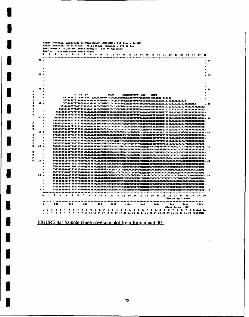
Range Coverae,. AMlituie Ve Time Delay JU DOW . 100 Time, . 24 ONYI Radr Location 51.44 II Let 79.1# W Lnn Bearing . 275.00 DogPeak .ue 0.200 MW Pulse Width . 120.00 NicrosecKoff 0.0 dUW Above Noise Floor

012 3 4 5 0 7 a 0 10 11 12 13 14 15 10 17 18 10 20 21 23 23 24 25 26 27 28

80 9

70 4 7

N77 88 99 cccc RiuUMP"" Ep -55 0000777 888 909 AAMAABUDDICCCCCCDDDDD........ rtoaa x.... flUDU 111111

L - 55546647777888899999AAAAA38UDDCCCCCCDDDDD............... uOpG-UNUUUUohhiiixliaiaJJiaJ3J

1 80 *555448677778888899998AACCCCD3DCCCCCCDDDDDSIRUunypnFnncnnggMnnjIIIXz J~JJJJJ3JJJ.K...jj *00

9 S5 $66477788778080800 AACCCCBDCCCCCCCDDDDD....... .T:-GaG'uuzzuuni I IIIJJJJJJJJJXfKKIMKKKKKII-- SS555666077787778900A~AA00OCCBWC3CCCCCeCCCDDo .~YFF~ OflfOOflhUUUUU3IIIZIIIJ3JJJJJJJJKRUKKKKIIKIK-

555:S:: o6#6777 8777 8o: oaA~AmAD C BCCChCCCCCCCCCcC CDDC.., .. Z. Q U333U3UIIIIi3JJJJJJ KI R3Z I-

A7:78t -cccD 111j Mj

-0 S55SS666680775#777899AAABBUCD8DDCCBCCCCCCCCCDDDDD... *.*1. 1 doITCJJJKKXKKK

- 6 S55807750777889 AAAAUahUBCcCCChDDDDCcCuaZCeCCCCDDDDDLncc......,",.".... ZJJJJJJKZIIIIKKIIIKN-R 555S55555440077S47778999JJfA3CC33UflBDDDDDCCcc3R~CCCCC .711IZIJCJJJIIIKKflhIIIIKz-R3- 5S555555844477S47778P0,MAAIAAcUUBBDODDDDDCCZCCCDDDCISMOrrrPCCccC-iijKKKKKK.3

- 555S5558344977567771889 gaa9 aaaD~wnCCCRJccaCCDDDDC C wjxjaaa=20a SSS5555S866477S877788099 8AAAffDDDDDCCCC 4 30CDa 555555S5446677547778*989 U08aA~lfDODDocCCC-

- 5515535355407754777809PAPP gaAa8mnccccczcccccn DCRNBCCCCCCC

- 555555SS8844$77507778888888888 h2BBDD- 55S55555S4646775477789 8889959~

104 55555S53S66677S4777888888888£AMA----- - ------- S555555544847754777788888888AAAUDDDDC9C9C9D D-

ID SSSSSS046677S5777788480499988RAfDDDcccc1cn. - --------

- 5555555546647757777868811111 -------DDD c DccCcDDDDDD CCIZcccccc3GCCCCccCCCC0GDDDD-

----------------------------------- 4.----I---------------------*-------------,--1 2 4 6 78 910 It 12 13 14 15 10 17 18 18 20 21 22 23 24 25 24 27 28

Time Delay - mOan*------------------------------------------------------- *------ --;------------------ ;----------

0 200 400 00 s00 1000 1200 1400 140 1800 200 2200

Slant. Ramse - UK ymolt

1 2 3 4 S 4 7 6 010 11 121314 15 1417 18 10202122 23 242526027 28 20303132 33 3435 Pr~qjXzI

FIGURE 4a: Sample range coverage pl1ot from fortran unit 30

I 75

Range Coverage, Amplitude Vs Time Delay JUN 88N . 100 Time - 24 WOORadar Location 51.44 N Lot 79.16 W Lon Searing - 275.00 DogIPeak Po-e to 0.200 NW Pulse Width . 120.00 NicrosesRaft . 0.0 48W Abov. Nois Ploor

25 26 27 28 29 30 31 32 33 34 35 36 37 38 39 40 41 42 43 44 45 46 47 48 49 50 51 52 53

90 9 0

80. .803

70. 70A -

1 60 .991n 60T -KIKSKIKKKKXK0 -UIIIIRUXIKIKKKKo -.KnKIXKKKKKKKKXR

so *KX0UUaM50I

*KKUURIIIIKKK L

A -UKKK~lKI LL 00 83R -KIKKIIxxKIIKIKKZ LL 0000 83838 llo 0 -KKKKXKKKKKKXKKKRM LU PIP 000000413333333XIIIII 3.

A -AFKKKUKFKKKKRKIKRKMZ LLLL GoG RUSH flW01CfG33333333IIIIIIIII 3333II__ _ _ _ _ _

a 30 +KKJCI LLLLL afololloooi~luMER uuuuuU IUIIIIII III I 11 L333333.3KKKKXIKI=KYIKKIK. 30-KIZKKKKKKIXKKKKIZZZRELLLLT ,L..,OlrloafllWtfFl3333333333333333h!aanm iiiiliI III 1iiiiii3J33JJ3.KUKIKK11KI-

a -311133111K3K1333333LLLL' **...*FGGG009-oOGGOfl¶I-fl0003333333333m33u!I1! '11111113333331111K11111111KatI-

_ _ _IIIIIII__1__ _ _111 _ _ _ _ _

ý LLL~rrrrrrrrrfl333333U3333333U3ii2l2i222221xiiiix!Ljj333333JKKII3ua-S20 GQ ý 11111111120

,0000.~- gril IIXIIII

-=GGGMDOOnnop@o@@iooD. -10 0o0-n---- ...... IZIIIIIL73333I 11 Z33I-

- 3333000------------------------------------ -- ----L3 33 331 ------ ------ ------b------ ------ ------- -- --- ------ o : f l r- Z ! I U !I1"3 3 31 11

25 26 20 0DDDODDOOOO 29 3 1 32 334 3 3 7 3 3 0 4 2 43 44 45 46 47 48 .5 50 5 52 5

--------------------------------------------------------------- I-2000 2200 2400 2600 2800 3000 3200 3400 3600 3800 4000 4200

slant Range M1 2 4 G 8 A C 9 G 1 JI LN X0 PQ R8 TV VW X1 2Symbol To

1 2 3 4 S 6 7 8 9 10 11 12 13 14 15 16 17 18 18 20 31 22 23 24 25 26 27 38 28 30 31 32 33 34 35 Freq(KS)

FIGURE 4b: Sample range, coverage from unit 30. secv..d pa e3

763

U

URange Coverage. Amplitud• Ve Time Delay JUN SN . 100 Tmis . 24 am?Radar Lo•ation 52.44 N Let 71.16 V Lon gearing z 275.00 Degpeak p oer = 0.200 MW Pulse Width . 120.00 NicrosecRaff . 0.0 dOW Above Noise Floor

50 51 52 53 54 55 56 57 58 59 60 41 62 63 64 6S 66 47 68 69 70 71 72 73 74 75 76 77 78

00 . . 90

80 * 4.80

70 .70A -

N-

LI go* 60

,,m T

u

IIR

1 40 . 40

V -K

C -

II -

40 ., . 40

A -

V~-K

2 30 *KKKUIK3IK M. 30

R -XONIKOILI IIEKS-

1 20 4IIN KKKKZXKKKKK * 20

- KKKKIKXKIKKKKKXKRKKKKK

-UISZ I---KKKKKKKKKKK

U IK L * 10

--- K I K=KK KKKKK KK RK IK E L

-KKKK XXKK KAKKIKKXK RRKKKIKKKK LLL

-KIIIRK]K KKMIKKEKKKKKKKKKKKKKKK LLLL

0 *,IIKKKRKKKKRKKKXKKKKKKKKKKKKI= LLLLL * 0--- -------------------------------------------------------------------50 51 52 53 54 SS 56 S7 58 S9 00 61 62 63 64 45 44 07 40 41 70 71 72 73 74 75 76 77 70

Times Delay - agoo

----------------------------- ------------------- ; -------------- --------- I--------- I----------------------------------------

Slant Rang.- 30

1 2 3 4 5 6 7 4, 70 A 0 C D 3 F 0 0 I 3 K L N N 0 I? S T U V W I y Z 2yabol To

1 2 3 4 5 0 7 8 1 10 11 12 13 14 15 16 27 28 29 20 21 22 23 24 15 26 27 28 29) 30 31 32 33 34 3S Pr"q(U:)

U FIGURE 4c: Sample range coverage from unit 30. third page

U

UU

U ,v

2.4) FOR030: Oblique ionograms

These graphs present the same variables as the range plot, but in a different form. Theionograms can be generated in signal-to-noise (target return) or clutter-to-noise (sea/ground

return). The symbols composing the data in the figure represent the SNR/CNR for each

frequency and delay. The data on the bottom line ( zero delay) are the noise reference for

each frequency. The oblique ionogram is generated at each of two different scales in time

delay: 0 to 50 ms in steps of 1 ms (see figure 5) and 0 to 25 ms in steps of .5 ms (see figure

6).

18

I

Oblique ZOIWas CoER V, Rang/ftiom Delay And Frequency 17-DRC-1992 1ls34?rmemitter Location 51.44 K Let 79.16 W Lon Nearing . 275.00 DogJM BENl . 100 Tim. a 24 WT Treansmitter Peak Power a 0.2 Mega&att4 5 6 7 8 9 10 11 12 13 14 IS 14 17 18 19 20 21 22 23 24 25 26 27 28 29 30 31 32 33 34 35

SO 5 .......... . . . ......... 3 16 25 33 .............. . . . ............ So 4000

................... 7 19 35 32................S.........................11 30 35 30................

. . ............. 315 32 32 27 ... . . . ................ .... ............ 7 1 34 31 24 .......... . . . ............. .

45 * .... . . . ........ 11 23 35 30 19 .......... . . . ............ . . 45 .3600

I *............. 15 25 37 2: 14................ -

. ............ 19 26 39 26 5...............

. ........ . . . ........ 22 35 26 26 .............. . . . ............. -

. ........ . . ........ 1 26 37 25 20 ............ . . ..............

40 . ...... . .. . ......... 8 29 38 25 14 ............ . . .............. . . 40 .3200

B * .... . . ....... 15 31 40 24 6 . ............ ... ... . . ......... . .............. .

A 3 32 7.......... 8 37 2 17................. -

6 2 .7............... 19 31 39 23 8 ................................. .

T 3 . . . ..... . . ....... 21 34 41 21 .............. . . ................ . . 35 . 800 2

. ... . . . ...... 24 36 23 14 . . . 7 ... . . . . . ............. L

T .......... 27 33 23 . . . . 22 .............. . A

I . 5 29 31 22 . 5 37 .................* . .:.: . . . . . . 20 32 18 22 G 15 . .............. ....... ... ......... T

3 30 , . . . . . . . . 28 35 16 22 . 16 33 .......... . . . ............. . 30 . 2400

D . . . . . . .. 33 31 13 21 13 14 26 58 ........ . . . ............ . - R

* .. . 37 7122 333035 12 12 21 25 2. 37 5: ........................ . . . . . . . . ..... A

S+ . . . . . . 2 32 38 14 12 39 39 42 49 62 ........ . . . ............ . - 6

A 25 .. . . . . 6 36 11 16 . 44 45 56 54 63 .............. . . . ............ 25 2000 i

Y . . .. . . 21 30 36 13 18 .47 49 616 4 62 ........ . . . ............ . .

...... 18 31 36 16 16 .50 53 63 64 5S9 .......... . . . ............ N

2 .2.. 2 2 1 133 18 17 50 53 S7 65 GS 5S ... . . ........ . . . ............ . .

9 . 26 2632 21 .535564676150....... ..................... ............. . .L 0 . 14 27 30 32 34 53 56 59 66 59 57 36 ...... . . . ............ .. 20 1600 1

1 2 1 7 16 730 31 3 56:9 :3 68 60 47 23 .......... . . . ............. .

. . . 10 23 27 37 46 59 4.3 67 59 54 33 7 ........... . . . ............ 6

S . 13 43 26 63 1 5 7 32 65 2...... 41 If .. ............................ *

c * 15210 336 567 4632 ................. 0

IS . 7 20 33 47 1 3 St 6 3 7 47 5 3 43 30 . 5. ................. ................ IS 2300

26 6670 39 48 56 41 i6 47 5 3 26 10 4 S 2 ...... .. . . . ............ ...

1 15 1 44 5 10 31 6566 61 44 4 38 67 5 23 19 14 ........ . . . ........... *

. 21 3 7 5 58 63 47 47 5 4 35 23 33 31 29 12 . ...... . . . ............. . .# IS 9 22 44 56 62 66 67 SS 41 42 41 39 37 34 29 21 . . . . . . . .0*3 13 34 S4 14 44 34 83 •1 . . . . . . . . . . . . . .

S 7384 38• S 53 2 7 47 46 44 2• 3• 3 27 1 . . . . . . . .

+ 31 46 S3 60 64 57 54 5f 49 4 4 44 4 0 34 27 17 .......... . . . ............. .

+ 41 53 59 45 59 So So 58 50 40 45 41 34 26 14 .......... . . . ............. . .

. 4 57 64 60 St S SO 46 41 33 21 S . . . . . . . ..... . . . ......................... 00

S 5 : :1 5 ::;:57 5 3 .. 33 2........................ .

*65 90505 73 46 37..... 60 56 7 53 46 5 1it ......................... . . . .....................* S2 47 36 16 ........................... .

*164166164169170172173174175175176177177178179179180 . . . . . . . . . . . . . .*

6----------.----------------------------------------------------------------------------04 5 6 7 10 1112 131151171120122 43 24 5 27 28 27 30 31 32 33 34 35

Frequency-mIFIGURE 5: Sample oble am from unit 30. large scale

II

I

II

Oblique 1c0ogrem, C Ve PangelTime Delay And Frequency 17-D&C-1092 11.36

Tranesltter Location 51.44 N Let 79.16 V Lo<n Bearing . 275.00 DogJON3 03 . 100 Timis - 24 ON? ranaumitter Peak Poour . 0.2 Negawatt4 S 6 7 8 9 10 11 12 13 14 15 16 17 18 19 20 21 22 23 24 25 26 27 36 29 30 31 32 33 34 35

-"-- "'"---- ----- --'" "- ---- ----- ------'---; . .;; ; -;'; ; " -:-7 " "-:- ':'" ":":-- --- --, - -:"--'"-- • .o* .. ......... 2 6 34 11 16 .44 45 58 54 63........ .................. ................... 2000*...... ..... 2 29 35 13 17 45 47 60 64 62 .......... . . ............. . .

24 . . . . . . 21 30 36 13 18 47 49 61 44 62 .......... . . .............. . 24 -

* . . . . . 19 31 36 14 29 48 52 62 64 61 .......... . . ............. . .

* ... . .... 18 31 36 16 16 50 53 63 64 59 .......... . . ............. . .

* ....... 16 32 33 17 16 52 S6 6464 58 .......... . . ............. . . 1o00

2 2 2 21 21 33 18 17 50 53 57 65 65 55 .......... .. . ............ . . 22

4 . . . . 424 23 32 20 .52 SS 55 66 65 52 .......... . . ............. . 4

* .... 9 28 26 32 21 .53 55 64 67 61 S0. .......... . . ............. . . .11. . 2 28 28 32 22 51 54 58 65 59 59 42 . . . . . . . . . . . . . . . .

20 . . . 214 7 30 32 24 53 56 59 66 59 57 38 .............. . . ............. *20 *1600

a . 5 19 27 30 31 13 54 58 62 67 S9 51 33 .......... . .. . . ............. * -

L . 7 18 27 30 31 565S9 63 68 60 47 23 .......... . . ............. . .

A 1 . 1 234 27 30 31 .57 62 65 60 60 43 12 .......... ... . . ............. * -N 18. * 0 23 27 37 46 59 43 67 59 54 33 7 . . . . . . . . . . . . . . . . Is

T * + 112 26 41 49 55 60 64 68 58 452 122 .............. . . ............. *1400 8* . . .13 23 24 43 50 58 62 66 69 58 41 16 ............ . . . .. . . .............. L

S . 3 1524 31 46 53 60 63 67 59 50 36 10 ............ . .. . . .............. - A1 16 . 20 23 36 47 54 61 65 68 S7 46 24 .................. . . ............... 16 m

. G 19 28 39 48 56 62 66 68 56 41 12 ................ . .. . . . ..............

S2 0 33 42 S3 59 63 67 54 47 30 .................. . . ................ *1200

10 20 35 46 54 60 65 68 53 37 18 5 2 ................ . . .............. * R

D 14 18 20 3 48 56 61 66 67 S3 26 10 8 5 2 .............. . . ............. 16 - A

a . 16 25 41 S0 S 63 66 45 45 19 18 17 14 11 6 ............ . .. . . . ........... -

L * 15 28 44 53 40 65 67 46 28 28 27 25 2319 2 .1. ....... . . ............ . - GA + 15 35 47 55 42 67 67 49 30 30 29 27 25 21 16 . . . . . . . . . . . . . . . 2 000 RT 12 + 21 37 51 5 63 47 47 SS 35 35 33 31 29 25 19 . . . . .................... .. . .12

* . 11 17 40 53 61 45 67 54 37 37 37 35 33 30 26 1 ............... . . . ........... - w

N * 15 0 22 44 5 62 66 67 55 41 41 41 39 37 34 29 21 ........ . . ............ . -

I + 16 14 26 48 58 65 67 60 59 42 42 41 40 37 34 29 20 ...... . . . . .. . . . ........... - N

L 10 . 20 31 39 53 61 65 66 61 61 44 44 43 41 38 34 29 18 ............ . . . ........... * 10 * 000 1

I + 22 32 46 55 62 45 65 63 46 4S 44 63 41 38 34 29 16 ............ . . . ........... -

.*27 38 48 SO 5 3 0 6 55 5S 47 47 46 44 42 39 36 27 12 ............ . . ............ * -

a 2 043 51 59 64 45 56 S 8 48 46 44 44 36 30 21 .............. . . ............. .

C *31 4 5360 4 57 S7 656 49 48 46 4 0 34 27 17 .............. ............... a -

* 37 49 57 63 67 58 S6 S7 49d•8 46 43 30 33 24 12 ............... . 600* 41 53 59 65 S9 50 58 So 5 0 48 4S 41 34 26 14 . . . . . . . . . . . . . . . . I* 455 63 68 60 50 S9 S9 50 47 43 372•8 16 .............. . ..................

6 4 57 44 60 59S59 59 58 46 41 3321 5 ................. . . ................ + -

S3 41 68 60 59 00 S9 57 43 36 25 9. ................ . . .................. .

+ 596 S 61 59 60 So 57 S3 33 20 . . . . . . . . . . . . . . . . . . . . . . d0#

* 42 6 7 59 60 59 57 52 4 16 ........................ . . ....................4 .65 60 59 59 57 53 46 37 .................... . . .. . . ..................... *

. 66 58 SO 57 S2 44 32 15 ...................... . . ...................... .

. 60 58 37 53 46 35 19 . . . . . . . . . . . . . . . . . . . . . . . . .

. 57 55 50 41 27 S ........................ . . ...................... . . 200

2 52 473 6 16 ........................ . . . ........................ .. 2 -

* ...........................

* ,164• 416016170172173174275175176177177178179179180 .......... . . ............ . .

4 S 6 7 8 9 10 11 12 13 14 15 16 17 18 19 20 21 22 23 24 25 26 27 28 29 30 31 32 33 34 35 IFrequency-NR s

FIGURE 6: Sample oblique ionogram from unit 30. small scale

IUII

so I

2.5) FOR030: Combined mode/frequency rayset tables

This table presents the same information as the rayset tables in fortran unit 10.However, all frequencies and modes for which unit 10 raysets were generated arerepresented. The sorting algorithm is somewhat similar to the one used in the 'allmodes.dat'output. The important difference is that this table contains no interpolated values; certainapparent inconsistencies are possible. The intent behind the table is to organize only thoseraysets which contribute to the top of the envelope in the backscatter vs. range plots. Theinconsistency arises when the mode/frequency providing the strongest returns is changingrapidly in distance for small changes in elevation; change on the order of 100 km/degree issufficient. When this rapid change occurs, a weaker return from another mode/frequencymay be inserted into the table at the skipped-over range. The intent behind 'allmodes.dat'is to avoid this problem by filling every range bin with the appropriate value, occasionallyusing interpolation to achieve that end. See figure 7 for an example. Note that this table wastruncated at a slant range near 2600 NM, normally the table would continue to the longest

* slant range shown in the range coverage plots.

IIIIIIIII

II

jam 8EW . 100 TIME . 2•4 00? 27-DZC-1992 110343 LO03 WCATION 51.44 N LA? 75.16 W LON SHARING - 275.00 D03PUAX POKI&A ý 0.200 NYi PULOR WIfDTH - 120.00 NICROS•C

AV33RAOR/PUKU PW RATIO . 0.0 D3 033 PATH ENIHANCEMENT 6.0 DOINT•ORATION TIlR . 3.10 S&C (OR 4.9 DR)

2-1100 M330 T3M13 AMCG RITZ 0T*,R C-AR•IA T3-UK R4TH AD8 D•V 0P SAW Q-LW T-LOWS P-NEC CUR am - I 30IN UZ1 mm D03 -K D3 D00 DSM DO3I D0 us D3 D3 D0 D0 D3W D3 Do DUW

318 5.0 3.9 22.0 114 44.4 54.2 17.0 230.8 32.2 4.7 0.0 0.0 0.0 35.4 -99.1 45.0 2•.7 -140.1 3

324 5.0 4.0 21.0 114 44.8 56.3 17.0 231.3 23.0 4.4 0.0 0.0 0.0 35.9 -99.4 05.4 24.2 -140.1 3

393 6.0 4.5 17.0 114 47.2 56.1 17.0 234.5 21.4 4.3 0.0 0.0 0.0 34.2 -100.4 44.4 27.4 -142.1 3

457 7.0 5.7 15.0 122 48.7 56.1 17.0 237.1 14.9 7.2 0.0 0.0 0.0 32.6 -101.3 47.4 28.3 -143.8 •

381 7.0 4.0 13.0 23s 40.4 56.3 17.0 234.0 20.7 5.8 0.0 0.0 0.0 33.0 -102.7 67.0 23.7 -143.3 3

538 8.0 4.7 12.0 122 48.9 56.2 17.0 230.0 27.9 5.7 0.0 0.0 0.0 32.0 -102.6 67.0 28.7 -165.3 3

577 8.0 7.2 20.0 114 49.2 56.4 17.0 242.2 19.7 5.4 0.0 0.0 0.0 31.4 -104.7 45.5 34.1 -145.3 3

437 9.0 7.9 9.0 118 d0.8 54.4 17.0 242.0 27.3 4.0 0.0 0.0 0.0 29.5 -105.0 44.5 27.1 -144.• K

4a1 9.0 4.4 28.0 330 44.9 57.2 17.0 244.1 8.2 9.2 2.9 0.0 0.0 24.8 -107.4 64.1 24.0 -164.4 2

748 10.0 9.2 7.0 120 49.2 54.4 17.0 245.6 16.2 5.5 0.0 0.0 0.0 24.5 -107.9 44.5 25.2 -147.7 378S 20.0 9.7 0.0 116 48.2 S4.8 27.0 2•6.5 10.5 5.1 0.0 0.0 0.0 28.5 -109.• 03.0 23.3 -107.7 9

849 10.0 10.5 20.0 310 51.4 57.4 27.0 247.9 9.0 8.4 4.9 0.0 0.0 25.8 -107.1 45.5 25.1 -147.7 2

576 11.0 10.9 20.0 321 51.4 57.0 27.0 248.4 7.8 8.1 3.6 0.0 0.0 26.0 -106.4 47.3 27.3 -143.8 2

959 12.0 12.9 18.0 325 52.4 57.0 17.0 250.0 7.3 7.5 3.5 0.0 0.0 25.2 -246.7 47.9 27.9 -149.7 2

903 12.0 12.2 17.0 323 53.1 57.1 17.0 250.4 7.6 7.7 4.0 0.0 0.0 25.8 -107.1 47.4 27.5 -149.7 210•• 22.0 12.9 15.0 326 5•.3 57.3 17.0 251.5 8.3 7.3 5.2 0.0 0.0 27.3 -108.2 6•.• 26.1 -149.7 2

1080 13.0 13.4 18.0 377 49.9 57.2 17.0 252.0 9.8 3.4 1.8 0.0 0.0 21.5 -108.2 47.3 27.1 -170.4 2

1148 13.0 14.2 16.0 371 51.4 57.4 27.0 253.1 20.7 3.4 2.7 0.0 0.0 23.3 -109.3 44.2 25.8 -170.4 2

1161 14.0 14.4 14.0 384 51.5 57.3 17.0 253.4 9.4 3.3 2.9 0.0 0.0 21.2 -208.0 45.3 28.0 -272.4 2

1253 14.0 15.5 14.0 374 53.0 57.4 17.0 2S3.4 10.3 3.1 2.9 0.0 0.0 22.9 -109.4 47.0 26.4 -171.4 2

1300 15.0 16.1 14.0 393 53.6 57.3 27.0 255.3 0.2 3.3 2.1 0.0 0.0 21.0 -108.4 45.7 28.4 -172.2 2 I1330 15.0 14.5 13.0 345 53.7 57.4 17.0 255.7 9.4 3.0 2.4 0.0 0.0 21.5 -209.4 47.8 27.3 -172.2 2

1407 16.0 17.4 13.0 414 54.3 57.7 17.0 256.6 4.4 3.6 2.9 0.0 0.0 20.4 -205.5 49.0 23.3 -272.0 2

1429 24.0 17.7 12.0 401 54.5 57.7 17.0 256.9 9.0 3.2 2.4 0.0 0.0 21.1 -109.4 68.4 27.7 -172.9 2

1513 14.0 14.7 10.0 384 54.2 57.9 17.0 257.9 9.0 2.9 3.7 0.0 0.0 23.0 -112.3 6s.5 24.4 -172.9 2

1557 17.0 19.3 11.0 425 54.9 58.2 17.0 258.4 8.5 3.6 2.2 0.0 0.0 20.8 -110.4 68.1 27.0 -173.4 2

157• 17.0 29.4 40.0 400 S.3 S8.1 17.0 258.6 1.9 3.2 2.8 0.0 0.0 25.4 -117.2 57.3 26.6 -173.6 2

1547 17.0 20.5 1.0 384 52.3 54.3 17.0 259.4 10.9 2.9 2.3 0.0 0.0 25.4 -117.9 69.9 18.6 -172.9 2

1478 17.0 20.8 5.0 3904 53.0 58.4 17.0 259.7 9.8 2.8 4.3 0.0 0.0 23.3 -115.8 42.7 21.3 -173.4 2

1725 21.0 21.4 9.0 436 54.5 58.5 17.0 240.2 8.5 3.6 2.7 0.0 0.0 21.3 -113.1 64.1 24.6 -174.2 2

1401 15.0 22.3 7.0 409 52.4 S8.7 17.0 240.9 9.3 2.9 4.1 0.0 0.0 22.5 -117.3 42.5 20.2 -174.2 2

144s 18.0 23.1 6.0 403 51.1 58.5 27.0 261.S 9.7 2.7 4.0 0.0 0.0 23.7 -220.0 59.1 17.3 -174.2 2

1910 17.0 23.4 5.0 359 47.9 55.9 17.0 242.0 11.2 2.1 4.4 0.0 0.0 27.1 -124.4 S2.1 10.2 -173.4 2

1927 19.0 23.9 7.0 452 53.0 S5.9 17.0 242.2 8.5 3.7 3.3 0.4 0.0 21.9 -117.1 42.4 20.7 -174.5 2

2017 19.0 25.0 5.0 424 48.7 59.1 17.0 242.9 9.2 3.0 4.4 0.0 0.0 23.3 -123.4 S.3 14.2 -174.5 2

2027 15.0 25.1 4.0 3904 45.5 9.1 27.0 263.0 10.5 2.4 4.2 0.0 0.0 25.5 -128.8 5$.3 5.2 -174.2 2

2090 19.0 25.9 4.0 414 45.7 59.3 17.0 263.5 9.5 .2.8 5.2 0.0 0.0 24.0 -127.7 52.5 9.5 -174.8 22167 13.0 26.8 19.0 394 dt.3 60.3 17.0 20•.1 22.3 8.4 3.5 0.0 0.S 40.• -137.1 38.5 -•.• -170.• 2

2159 20.0 27.1 5.0 482 49.1 59.5 17.0 324.3 8.4 4.0 3.5 0.5 0.0 22.7 -123.9 5•.4 13.9 -175.4 2

2228 20.0 27.4 4.0 442 45.8 509. 17.0 344.4 6.7 3.6 4.3 0.0 0.0 23.1 -227.9 52.4 9.9 -175.4 2

2294 20.0 28.4 3.0 451 39.4 59.7 27.0 245.1 9.0 3.3 4.8 0.0 0.0 23.4 -134.8 4S.S 2.4 -175.4 2

2371 24.0 29.4 17.0 403 51.0 40.4 17.0 265.7 22.4 8.6 2.4 0.0 0.6 39.6 -136.4 39.9 -3.5 -171.4 2

2423 14.0 30.0 14.0 390 51.8 40.5 17.0 264.1 22.3 5.4 3.4 0.0 0.4 41.2 -137.4 39.0 -4.5 -171.4 2243• 20.0 30.1 2.0 •02 33.8 59.9 17.0 266.2 12.4 4.1 S.7 0.0 0.0 28.8 -146.7 33.6 -9.4 -175.• 2

2499 14.0 30.9 15.0 393 52.4 40.4 17.0 206.6 23.3 5.2 4.4 0.0 9.9 52.3 -145.4 28.0 -15.6 -171.4 2

FIGURE 7: Sample combined freuency/modes table.

IIIII

I

I2.6) F0R032: Single frequency range plots

These graphs present the backscatter return vs. range for each frequency. They can be5 generated in signal-to-noise (target return) or clutter-to-noise (sea/ground return) vs. groundor slant range. The symbols composing the filled curve in the figure represent the mode withthe highest SNR/CNR according to the key at the bottom of the figure. This figure may becontinued for up to three pages if the predicted radar performance demands it (See figure8a,b). Fortran unit 30 has a similar figure, differing only in that all frequencies run areincluded, and the symbols used represent frequency instead of propagation mode.

IIIIIIIIIUII 3

II

Rlange Coverage. Amplitude V. Time Delay JU P3R - 100 Time 24 aS? PFrequeny - 13.000 K0Z 17-DBC-1992 11.36

Rladar Location 51.44 N Let 79.16 V Lon Searing . 275.00 Dog AWTTTP 12 IPeak Power = 0.200 Megawatt Pulse Width - 120.00 microaecRef f 0.0 dR Above Noise Level Of -175.5 d•W

0 1 2 3 4 S 6 7 8 9 10 11 12 13 14 15 16 17 18 19 20 21 22 23 24 25 26 27 28

------- -------------------------------------------------------------- 4------4-----------*,0 . Igo + 90

800. 80 I

70* 70A1N-

I -22222222L - 222222222221 40 , 22222222222222 * G0

T - 2 222222222222222223 a3 222222222222222222222

D & 3131 2222322222222222222222

S31133 2222222221122222222222

s0 * 3211231 2222222221112222222222 * S0

31313*33 2222222221111221122.222C -*33** 3 R3U2222222221111122222222 IN -*.....*******3U3M22222222221111112222222

.-* **,22221222222221111111222222

40 ................ . 22.. r.2322222221111111222222 . 40

A -... . .................. 11222223••22222111111122222I

8 -............. *11222231ZM222211111111122222 22222 --............. ,*111231129M2221111111122222 222222222-

V .. ....................... 3Illl*R M2222111111122222 222222222-

3 30 ............. ,11111*]3r1221111111222222 322222222. 30-............. *111111*I-33221111111122322 222222222-

3 -.............. 11111113313]221111111122222 222222222-

* - .. .. ... .. ,21112111 - m221111111122222 222222222-.. . . ..................... 111111111932221111111122222 3an 222222222-

F 20 *.... ...................... 1111111111Uin11111111322 333 222222222. 20-......... **....,111111111111331111111222 i 222222221--**0"**eeeeeee***** ..*****1111111111111311111122222 1mZ 222222111-

- I .. XR111111121 11311111122222 222221111-

C*....****e.e....... llll1111.11111122222 222221111-10 .......................... 22222111111 ... 1RU1111132223 123222222333231111* 10

-............. *,*1111111 -2*212231111122222 31lnn 13n3n133l33 222221111-t.tte.t.........1112222111111111. 311122

-* * * . ,,,111111X11CC**C*3t111122222 221111-

-... .... ... ,.,1111111. 311122222 313113313U33122221111-. . ............................. 1111211111 . 33=111,23222 3....2221111.-

---------------------------------------------------.----------------------------------------------------------

0 1 2 3 4 5 4 7 S 9 10 11 12 13 14 15 1f 17 18 19 20 21 22 23 24 25 24 27 28Time Delay - alac

---------------------------------------------------------------------------------------.--------------------

0 200 400 400 S00 1000 1200 1400 1400 1800 2000 2200Slant Rag - MW

FIGURE 8a: Single frequency range coverage from unit 32 (first page)

IIII

UI

Ran" CovYerg.e Amplitude Ve Time Delay JUN SSN - 100 Time . 24 GWTI Frequency . 13.000 UU: 17-D&C-0192 11.34

Radar Loctio 51.44 N Let 79.14 U Lon -earing * 275.00 Dog ANI7YrP 12Peak Pow-e• 0.200 4 egawatt pi•ole idth . 120.00 aicroaecDoff a 0.0 dc, Above Noise Level Of -175.5 dsw

25 24 27 28 29 30 31 32 33 34 3S 36 37 38 39 40 41 42 43 44 4S 44 47 48 49 50 51 52 53

-----------------------------------------------------------------4----------------- ..................I00 . 0

I "0. *5

90 9 0

70 . * 703APN

L

I G .40

50 *0A

* 5

C -

I - 222220 -

40 + • 40

V 2-2223 30 2222222222222222

- 22222222222222222R -0 222222222222222222

'-2222222222222222222

- 22222222222222222222F 20 *222222222112222222222 20

- 22222222111112322222222

- 22222211111111222222222

-322222111111131112222222I - 22222111111111111122222210 4222221111111111111222222 21"-3 2222211111111111112222222

- 333322211111111111112222222-32Mt22211111111111112222222

-W W 22212111211111122222222

* *EM 222111111111111t222222222------------ ,------------------------------- .------------------- -. ----------- ---------------------. ---.

2S 26 27 26 21 30 31 32 33 34 35 34 37 38 39 40 41 42 43 44 45 44 47 46 409 50 51 52 53

Tlme Delay - muec

200 2200 2 0 00 21800 3000 3200 3400 3600 3600 4000 4200Slaret Aum** - MN

FIGURE 8b: Single frequency range coverage from unit 32 (second page)

I -III* 85

II

2.7) FOR032: Single frequency angle coverage

These graphs present the rayset geometry in a different form. The mode is plotted asa function of elevation angle and time delay. The leftmost curve for each mode is the one-hop; the hop increases by one for each curve per mode, read left-to-right. The modesymbols are '*','1','2', and '+' for the sporadic-E, F,, F2, and over-the-MUF modes,

respectively. The figure may be continued up to three pages if necesssary (See figure 9a,b).

IIIIIIIII

II

I

II

Angle Coverage, Amplitude V. Time Delay JU 8SON . 100 Tlme . 24 GUT Frequency - 13.000 Niz 17-D•C-1992 11.36

Radar Location 51.44 N Let 79.16 W Lon Searing . 275.00 Deg ANTM 12leak Vo er a 0.200 Megawatt Pule* Width = 120.00 alcrosecleff 0.0 dB Above Mole Level Of -175.5 dSN

m0 12 3 3 5 s s 7 8 9 10 11 12 13 14 15 16 17 18 19 20 21 22 23 24 25 24 27 28

---------------------------------------------------------------------------------------------------------------------U ~~45. 4

40 . • 40

A 35 . 3S

m3* 303 3- .

D - .

8 25 * 2 .25

m 2 2-

• .5 22 2S - ** 2 2

20. * 2 2 + 20

m 2 2

• 5 2 2

- * 2* ** 2 2 12

1i. - * 2 15

• o 2

10• 1 1-. 1010. 1 I

1* 3 -•*

5 * 3

21222 2 5 .4272

Slant Reang - EN4

m FIURE9a:Sample single frequency angle coverage from unit 32

llIIm S7

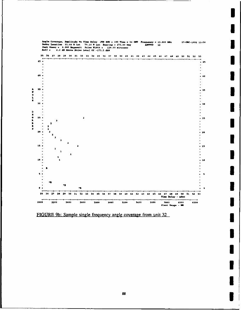
AngI. COVerage. lM~1ItUd Ve tifte Delay JUN9 ZEN0 - 100 Time m 24 ON? Frequency a 13.000 US& 17-DILC-19,2 11.30Radar L~oation 51.44 N Let 79.16 V Lon Rearing - 275.00 Deg AXUTYP 12IPeak Power . 0.200 Megawatt Pu.lse Width = 120.00 mlcromecAeff 0.0 dB Above Noise Level of -175. dEW

25 26 27 28 29 30 31 32 33 34 35 36 37 30 39 40 41 42 43 44 45 46 47 48 49 50 51 52 53-- ---- --------------------------------------------------------------------.---------------------------------

45 , I

A 35* 35

30 30

2 2A - 2

20 - 23-2 I3 - 2

20. 2

- 2

-5 2 IS

- 1

- 1

-------------------------------------------------------------------------- ,--------- ----------

25 24 27 20 29 30 31 32 33 34 35 36 37 36 3t 40 41 42 43 44 45 44 47 46 49 50 St 52 53

Time Delay - Base------ -- .-.---------------------------------------------------------.------------------------------ 4

2000 2200 2400 2600 2600 3000 3200 3400 3600 3600 4000 4200

FIGURE 9b: Sample single frequency angle coverage from unit 32

II

2.8) ALLMODES.DAT: Combined envelope rayset tables

This table presents the same information as the rayset tables in fortran unit 10 and thecombined raysets of fortran unit 30. However, all frequencies and modes for which unit 10raysets were generated are represented, and, although the sorting algorithm is somewhatsimilar to the one used in the fortran unit 30 output, this table contains interpolated values.

The sorting algorithm traces the envelope of each mode, rather than the discrete raysets.Values of the interpolated envelope then fill range bins that would otherwise fall through toa weaker return. The intent behind the table is to organize only those raysets whichcontribute to the top of the envelope in the backscatter vs. range plots. The match is goodeven when the mode/frequency providing the strongest returns is changing rapidly in distancefor small changes in elevation. When this rapid change occurs, a weaker return from anothermode/frequency will be covered by the envelope of the strongest return. The items in the

table are similar to the fortran unit 10 items, with two exceptions. The column labelled'NOISE' does not appear in fortran unit 10 rayset tables because the noise reference is3 constant for constant frequencies. This table may have different frequencies, hence the needfor a noise reference in the body of the table. In the last column (unlabelled to save space)is a mode symbol. This is identical to the mode symbols in the fortran unit 10 raysets,

except when the rayset has been calculated by interpolation of the envelope. In this case themode symbol will be ' - '. All raysets not marked as interpolated are actual, calculated

raysets that match raysets in fortran unit 10. See figure 10 for an example.

IIIIIII

II

J a m 100 TUM . 24 GMT 17-DZC-1092 11.36RDAAR LOCATIOI 51.44 X LAT 79.14 V LOU HRARING . 275.00 DZGPEAK POWER . 0.200 MW PULSE WIDTE . 120.00 MICRO.CAVILAG•/P•AZ PU RATIO . 0.0 DR O5" PATH &M6AICENENT - 6.0 DRINTEGRATION TIME * 3.10 SEC (OR 4.9 Dig)

8-REQG FZQ TIME ELAJNG RITE GTGR CARRA TARSA •4TH ASS DRV OBF REF G-LOS T-LO082 P-REC C SME E NOIS E

NEZ MSaRC DOG KM DR DOPEN D DSM DRM DR DR DB DR DR DR DRE DR OR DI

290. 5.0 3.59 23.0 110. 44.2 55.8 17.0 229.2 0.0 0.0 0.0 41.9 0.0 41.5 -109.5 60.4 21.6 -165.0 S313. 5.0 3.87 23.0 119. 44.2 56.1 17.0 230.S 21.4 7.5 0.0 0.0 0.0 35.4 -99.1 65.5 24.8 -160.1 E383. 6.0 4.74 18.0 115. 47.2 56.0 17.0 234.0 20.5 7.1 0.0 0.0 0.0 34.1 -100.0 67.0 28.0 -162.1 E

404. 6.0 5.03 16.0 114. 47.2 54.3 17.0 235.1 22.3 5.9 0.0 0.0 0.0 34.7 -101.4 65.6 26.4 -162.1 2457. 7.0 S.66 15.0 123. 48.7 56.1 17.0 237.1 28.9 7.2 0.0 0.0 0.0 32.6 -101.3 67.4 28.3 -163.8 2535. 8.0 6.47 12.0 122. 4 1.5 50.2 17.0 240.0 17.9 6.7 0.0 0.0 0.0 31.1 -102.6 67.6 28.4 -165.3 •

552. 0.0 4.83 11.0 117. 49.4 54.2 27.0 240.4 28.8 5.8 0.0 0.0 0.0 31.1 -103.2 67.0 27.7 -105.3 3

637. 5.0 7.89 9.0 119. 45.8 56.4 17.0 242.9 17.3 6.0 0.0 0.0 0.0 25.8 -105.0 44.5 27.1 -166.6 R870. 9.0 8.30 8.0 116. 49.2 56.6 17.0 243.8 18.2 5.3 0.0 0.0 0.0 29.9 -106.5 45.0 25.4 -164.6 E

722. 10.0 8.93 29.0 350. 45.9 57.0 17.0 245.0 6.7 10.5 1.4 0.0 0.0 25.4 -107.0 O5.4 25.6 -147.7 2784. 10.0 9.73 23.0 311. 48.3 57.1 17.0 246.5 8.1 8.3 3.5 0.0 0.0 26.4 -107.0 65.7 25.6 -167.7 2842. 11.0 10.42 22.0 332. 49.4 56.9 17.0 247.7 7.2 8.6 2.8 0.0 0.0 25.2 -106.9 66.8 26.9 -168.8 2858. 11.0 10.62 21.0 327. 50.4 57.0 17.0 248.0 7.5 8.2 3.2 0.0 0.0 25.4 -106.4 67.3 27.3 -168.8 2139. 12.0 11.63 15.0 335. 51.8 57.0 17.0 249.6 7.0 8.2 3.1 0.0 0.0 24.8 -106.6 67.9 27.9 -169.7 2160. 12.0 11.88 18.0 329. 52.4 57.0 17.0 250.0 7.3 7.8 3.5 0.0 0.0 25.1 -106.7 67.9 27.9 -169.7 2

1045. 13.0 12.13 20.0 313. 48.6 57.1 17.0 251.5 9.1 3.9 1.1 0.0 0.0 20.6 -108.2 67.3 27.2 -110.6 21060. 13.0 13.12 19.0 384. 49.2 57.1 17.0 251.7 9.5 3.6 1.4 0.0 0.0 21.0 -108.1 67.4 27.3 -170.6 2

1110. 13.0 13.73 17.0 373. 50.7 57.3 17.0 252.5 10.3 3.3 2.2 0.0 0.0 22.2 -108.6 67.0 26.7 -170.6 21162. 14.0 14.38 17.0 354. 51.0 57.3 17.0 253.3 9.1 3.5 1.S 0.0 0.0 20.6 -108.0 68.3 28.0 -171.4 2

1213. 14.0 15.01 15.0 375. 52.4 57.4 17.0 254.1 9.9 3.2 2.3 0.0 0.0 21.9 -108.5 67.8 27.4 -171.4 21278. 15.0 15.82 15.0 404. 52.9 57.3 17.0 255.0 8.8 3.6 1.6 0.0 0.0 20.5 -108.3 48.8 28.5 -172.2 2

1300. 15.0 16.05 14.0 394. 53.6 57.3 17.0 255.3 9.2 3.3 2.1 0.0 0.0 21.0 -108.4 68.7 28.4 -172.2 21375. 15.0 17.01 12.0 381. 53.8 57.5 17.0 256.2 10.1 3.0 3.2 0.0 0.0 22.8 -110.7 66.4 25.9 -172.2 21403. 14.0 17.37 14.0 433. 54.2 57.7 17.0 256.4 8.2 4.2 1.4 0.0 0.0 20.3 -108.7 69.1 28.4 -172.9 21467. 16.0 18.15 11.0 353. 54.4 57.8 17.0 257.4 9.4 2.9 3.0 0.0 0.0 21.9 -110.7 67.1 26.3 -172.9 21524. 24.0 18.73 10.0 387. 54.2 57.5 17.0 257.9 9.9 2.9 3.7 0.0 0.0 23.0 -112.3 65.5 24.6 -172.9 21553. 17.0 10.22 12.0 447. 54.5 58.1 17.0 258.4 8.1 4.2 1.7 0.0 0.0 20.5 -110.0 66.5 27.4 -173.6 21600. 17.0 15.80 13.1 491. 54.5 58.2 17.0 258.5 7.7 5.6 1.3 0.0 0.0 21.1 -111.3 67.2 26.0 -178.5

1650. 17.0 20.42 13.5 520. 54.4 58.4 17.0 259.4 7.6 6.7 1.2 0.0 0.0 22.0 -112.7 65.8 24.5 -178.5 -

1711. 18.0 21.28 10.0 460. 55.4 58.5 17.0 260.1 8.1 4.2 2.1 0.0 0.0 20.9 -111.8 67.4 25.5 -174.2 21767. 18.0 21.84 11.0 504. 55.4 58.6 17.0 260.4 7.7 5.5 1.4 0.0 0.0 21.4 -112.4 66.5 24.5 -174.2 2

1800. 18.0 22.28 11.1 520. 55.4 S8.7 17.0 240.5 7.7 6.3 2.6 0.0 0.0 22.1 -113.6 45.6 23.5 -179.1 -1850. 18.0 22.00 11.3 545. 55.3 S8.8 17.0 201.3 7.6 7.5 1.S 0.0 0.0 23.2 -115.0 64.1 22.3 -170.11525. 15.0 23.82 8.0 481. 54.3 58.5 17.0 262.1 8.1 4.3 2.6 0.0 0.0 21.5 -115.4 64.3 22.3 -174.8 2

1104. 21.0 24.56 5.0 532. 55.2 59.1 17.0 262.6 7.7 5.9 2.1 0.0 0.0 22.2 -115.6 64.1 22.0 -174.8 22021. 20.0 25.01 8.0 514. 54.5 55.2 17.0 262.5 7.4 8.8 0.0 0.0 0.0 22.7 -117.1 63.2 21.1 -175.4 *2070. 18.0 25.61 12.0 455. 55.3 59.3 17.0 263.3 7.3 12.5 1.2 0.0 0.0 27.5 -1 1.3 57.9 15.5 -174.2 2

2100. 15.0 25.99 3.5 414. 45.0 55.3 17.0 263.6 9.6 2.8 5.3 0.0 0.0 24.1 -128.5 51.2 8.4 -175.7

2111. 20.0 27.12 6.0 516. 52.4 55.5 17.0 264.3 8.1 4.0 3.2 0.0 0.0 22.7 -120.6 59.7 17.2 -175.4 22200. 20.0 27.23 6.1 521. 52.5 59.5 17.0 264.4 8.0 5.1 3.1 0.0 0.0 22.8 -120.7 59.6 17.1 -180.32250. 20.0 27.85 4.4 551. 52.5 59.6 17.0 264.8 7.9 5.9 2.9 0.0 0.0 23.3 -121.1 55.2 16.6 -180.32343. 20.0 25.00 7.0 607. S3.7 59.8 17.0 265.5 7.7 7.5 2.6 0.0 0.0 24.3 -121.8 58.4 15.6 -175.4 22350. 20.0 25.08 2.6 456. 37.4 59.8 17.0 265.5 10.4 3.6 5.2 0.0 0.0 25.7 -139.5 40.7 -2.0 -180.32423. 14.0 29.19 16.0 397. 51.8 60.5 17.0 266.1 22.3 8.4 3.4 0.0 0.6 41.2 -137.4 39.0 -4.5 -171.4 222470. 14.0 30.57 21.0 494. 48.4 60.7 17.0 266.4 18.3 16.0 0.7 0.0 0.5 42.0 -141.8 34.5 -9.1 -171.4 32

2500. 14.0 30.54 21.1 503. 48.3 60.7 17.0 266.6 18.2 17.0 0.7 0.0 0.5 42.9 -142.5 33.5 -10.2 -176.4 -

2575. 21.0 31.52 3.0 551. 40.1 60.2 17.0 267.2 11.1 5.4 4.2 0.0 0.0 27.4 -140.3 40.4 -2.4 -175.5 22432. 22.0 32.57 2.0 531. 34.0 60.3 17.0 247.5 11.4 5.2 4.6 0.0 0.0 27.7 -146.5 33.9 -5.4 -175.5 2

2658. 15.0 32.89 14.0 405. 53.4 60.4 17.0 267.7 21.6 8.0 3.5 0.0 9.5 49.5 -146.2 31.0 -12.5 -172.2 22

2737. 15.0 33.87 13.0 400. 53.7 60.5 17.0 268.2 22.7 7.5 5.0 0.0 0.7 42.8 -135.8 37.3 -6.2 -172.2 22

2750. 15.0 34.03 22.t 350. 53.7 40.0 17.0 268.3 22.8 7.9 5.2 0.0 0.7 63.1 -140.1 37.0 -6.6 -177.1

2840. 14.0 35.14 14.0 440. 54.2 60.7 17.0 248.8 15.4 5.5 2.5 0.0 0.7 38.6 -136.1 41.7 -2.0 -172.9 22

2861. 14.0 35.41 13.0 423. 54.3 40.7 17.0 245.0 20.3 8.4 3.4 0.0 0.7 39.4 -134.9 41.0 -2.8 -172.5 222900. 14.0 35.89 15.2 478. 53.2 40.8 17.0 264.2 18.3 12.1 1.7 0.0 0.7 39.3 -138.0 39.8 -4.0 -177.8 -

2150. 16.0 36.51 15.6 456. 52.9 60.9 17.0 264.5 18.0 13.3 1.5 0.0 0.6 40.0 -139.3 38.6 -5.4 -177.83004. 14.0 37.17 16.0 515. 52.6 41.0 17.0 269.8 17.7 14.7 1.3 0.0 0.6 40.8 -140.6 37.2 -6.8 -172.9 22

3050. 16.0 37.75 10.6 405. 54.3 41.0 17.0 270.1 22.7 7.5 6.5 0.0 0.5 44.1 -142.4 35.4 -8.6 -177.8

3139. 17.0 38.85 12.0 453. 54.9 41.1 17.0 270.6 15.1 9.4 3.2 0.0 0.8 35.0 -137.6 40.9 -3.3 -173.6 22

3186. 17.0 39.43 13.0 485. 54.6 61.2 17.0 270.8 18.2 11.3 2.3 0.0 0.8 39.1 -1306.3 40.2 -4.0 -173.6 22

3200. 17.0 39.40 13.1 450. 54.6 61.2 17.0 270.5 18.2 11.6 2.3 0.0 0.8 39.3 -138.6 39.0 -4.3 -178.59250. 17.0 40.22 13.3 506. 54.5 61.3 17.0 271.2 18.0 12.8 2.1 0.0 0.8 40.1 -135.6 38.9 -5.4 -178.53300. 17.0 40.84 13.5 521. 54.4 41.4 17.0 271.4 17.8 13.9 1.9 0.0 0.7 60.8 -140.6 37.9 -6.5 -178.5

3358. 17.0 42.06 14.0 552. 54.3 61.5 17.0 272.0 17.4 16.1 1.6 0.0 0.7 42.3 -142.6 35.9 -8.6 -173.6 22

FIGURE 10; Sample ALLMODES.DAT combined envelope table. I

I90!

I 2.9) F0R034: Diagnostics

This file contains diagnostic and intermediate output, used to debug the program. It is notintended to be generally useful and is subject to change. Since the contents of fortran 34 areconstantly changing no attempt is made here to document them fully. Suffice it to say that thislarge and generally useless file need not be generated; just don't use 'printout 3'. Now, with

that said, there is a potentially useful table at the top of this file. It lists most of the values ofthe input parameters. If you have difficulty with a keyword, at least you may be able todetermine whether it's getting in correctly. Unfortunately, not all input keywords and their

values are reported. See the following figure II for a sample of the input echoed in unit 34.

IIIIIIIIIII

I •

II

IT1LAT * S.44000 $1.44000.ZXUiauo * 71.:4000 7.10800

m S.00000 28.00000 1.000000TP•P Z . 0.20:0000 53.01030ZIU E • 1205.0000 120.0000 020

C * 3.100000

AWT -1.2 12TIM * 24.00000 0

TEk 1991

,+,,.Y . 10.000o0FLUX * 115.0030KP = -1.700000

]PO1 * 1.000000r11u n 1.000000F0 RM 0.7000000

BAUnM DYi * 4333.333

1T 1.000000KIAC = 5.000000L.IC.IU * 0

1CWOT - 9.9999998*-03*c1ut , 9.9540063-03.1*813 .* 7.000o0

ILANT 3*JUI3 PLOTSWORK" EUMUIY PRNDTIOUT"INDIDXV1UAL rRUOMUMCT PRINTOUT"* DIAOMKTIC PRDIrOUT U

< more cryptic data vould follow

FIGURE II: Partial output from unit 34: echo of input values

IIIIIIII

92!

IIIIUIIIU PART III

S~FORTRAN implementation details

IIIIiIII

U

I1.) Program description of RADARC

The purpose of part III is to walk the reader through the flow of RADARC, and to providesuch program information as will facilitate the efforts of any user who wishes to understand theimplementation details. A brief description of the function each routine performs accompaniesthe implementation information. These comments will be general enough to inform the reader' who is unfamiliar with programming or specifically with the FORTRAN language. The readershould be forewarned that the structure is complicated and much care should be taken whenchanges to the code are considered.

I Chart I is a diagram of RADARC showing the general flow of the program calls. There arefour main subroutines that control the flow of RADARC. A short description of each of these"main" subroutines is presented here; descriptions of the rest of the subroutines follow. Themajor output is generated in subroutines AMPALL, SNRPLT, OPLOT, SETPLT and VPLOT.

IONGEN Retrieves the input data supplied by the user and developes the ionosphericparameters for the three layers (E, Fl, and F2).

BAKSCT Backscatter control routine that calculates the vertical ionograms, reflectrix,oblique paths for all frequencies, and calculates and organizes some output.

t RADAR Takes the oblique information from BAKSCT and evaluates the systemparameters, losses, and calculates sporadic-E modes and losses.

I SLANTY Gathers all information on modes, losses, and environmental noise and putsit in the form of the radar equation; it also gets the spread Doppler clutter by

* a call to ABILITY.

9IIIIII 9

II

1.1) List of program routines with a short description

RADARC - Main program ',controls all functions, sets named common, some data;gets date/time, and set )r function to avoid certain unwanted warnings duringexecution.

IONGEN - Called by main program RADARC to determine input and calculate ionospheric Ivariables.

PRESET - Sets predefined program control variables; used in lieu of block 3data.

READIN - Reads the program control (input) variables from user input file on FORO0 1.

F ICOF - Determines data base and calculates F l-layer parameters from monthly numericalcoefficients

REDMAP - Reads the longterm ionospheric data file.

GEOM - Calculates geographic and geomagnetic parameters

CORDY - Calculates latitude and longitude of a point, given distance and azimuth from aknown point. 3

MAGVAR - Calculates magnetic field and gyro-frequency.

MAGFIN - Cacluates the three magnetic field vectors. UMAP - Digitized map of the land boundries of the world 3VERTIM - Calculates the time variation of ionospheric variables for sample areas.

ESIND - Calculates the sporadic-E MUF by a call to VERSY (see above). Data for the F,-layer was calculated in REDMAP (see above). 3

TIMVAR - Calculates time dependence of the numerical maps of ionospheric variables.

EFIVAR -Calculates E and Fl-layers ionospheric variables. n

VERSY - Calculates geographic variation of the numerically mapped ionospheric variables. 1I

"96

YMAP - Calculates the F2-layer semi-thickness from numerical coefficients

F2VAR - Uses F2-layer numerical maps calculated by VERSY (see above)

3 POLARC - Determines the polar corrections for auroral oval and trough calculations whenrequested in the input file

CGMTIM - Determines corrected geomagnetic time by entry point to subroutine CLOCKS

3- JULIAN - Converts Gregorian date to Julian day; day set for 15th of month

GYRE - Computes solar ephemeris data of prediction time, in particular, right ascension,5 declination of sun and Greenwich SID time

GIMBAL - Updates the solar emphemeris data computed by GYRE to sidereal, correctedSgeom agnetic, and earth centere-d dipole m agnetic tim e.

GEOMAG - Converts a point given in geographic coordinates to the correspondingcorrected geomagnetic coordinates

5 DIPOLE - Converts from geographic coordinates to earth centered dipole system

COSD - Computes great circle distance between points on earth

BCKSCT - A call to INPUT obtains previously generated ionospheric parameters neededto calculate the electron density profile. INPUT calls INLEC, which reads electrondensity profiles or virtual heights (ionograms). This is a seldom used option.

3 ZERO - (Re)initializes data arrays.

LECDEN - Calculates the electron density profiles (parabolic layers) from the parametersread in by INPUT.

GENION - Integrates the true height electron density profiles to obtain a virtual heightprofile that will be used for all calculation from this point forward

5 ALOSFV - Calculates the deviative loss factors from the virtul height profile.

FOBBY - Generates the reflectrix and determines oblique frequencies.

CUSPFV - Computes values of the frequency/height parameters about the cusp and puts inreasonably smooth values that resemble those scaled from actual ionograms.

* 97

I

HEAD99 - Writes header information to FOR099.DAT for use on the combined raysettables in FOR030 and ALLMODES.DAT.

AMPALL - Plot routine that sets up line printer character plots of signal-to- noise ratio forall frequencies and all modes of propagation.

SNRPRT - Routine that sets up variables and prints the tabular output IOPLOT - Plots the oblique ionograms for all frequencies and power levels.

READ99 - Generates and prints the combined rayset table in FORM30. IREA992 - Generates and prints the combined rayset table in ALLMODES.DAT. n

RADAR - Backscatter control routine. Searches the oblique frequency tables for thereflectrix with constant frequency. If over the MUF these losses are calculated. Thenthe backscatter returns are computed.

ANTOO - Table look-up of gains for the selected antenna nTARGET - Computes the target size in dB above 1 meter2 . iSELION - Selects the cloest control area to the ionospheric reflection. The ionospheric

description at this control point is selected to represent the spherically symmetric model !used over the that hop,which permits quick closed-form ray path calculations.

SELDST - Calculates all distances for iongoram generation ISETION - Determines the system losses. It calls SIGNT, a routine that permits a desired

sea or land backscatter coefficient to be used. Adjustments have been made to this Iroutine to deternimine losses over the MUF.

SIGNT - Sets backscatter coefficient of earth's surface

ESDIS - Calculates probability of sporadic-E modes and determine losses

GAUSS - Solves the probability function

SLANTY - Finds the raysets for the E, Fl, and F2 layers. This routine gathers all resultsand puts them in the form of radar equation. I

CGMCS - Calculates corrected geomagnetic coordinates

98

II

SYSSY - Determines auroral loss from tables

CHANY - Calculates man-made and galactic noise level at receiver

I NOISY - Computes atmospheric noise levels from numerical maps

13 GENFAM - Determines frequency dependence of atmospheric noise

ABILITYV3 - Calcultes spread Doppler clutter by Elkins method

GLOSS - Calculates the reflection loss per hop for multi-hop paths

i CUSPIN - Calculates angles for the modified cusp values of E-F1 and f.-F2 layers

ESSNR - Determines raysets and all variables used in RADAR equation associated withsporadic-E modes.

BRING - Calculates bearing from one point on the globe to another, given the geographiccoordinates of the points.

i DTOG - Computes complex function of three variables

FPOK - Determines probability of spread Doppler

PEIR- Computes the value of E-layer clutter probability (F-layer clutter with entry point

3 PFIR)

MERFI - Inverse error function

PINCLY - Determines overall magnetic field by summation

3 SOLR - Updates orbital elements of of epoch

I FKEP - Calculates true anomaly for Julian day

XFR3 - Computes rotation matrix element

I SETPLT - Plot control routine that sets up variables to be plotted

5 ALLFREQ - Plots range vs amplitude showing which frequency was best at each range

intervall

1 9

II

AMPLOT - Same as allfreq, but shows best mode at each range interval

ESTERP - Sets indicies for sporadic E-layer printer plots

INTERP - Sets indicies for regular layer printer plots (E,FI, and F2) UCPTERP - Sets indicies for plot cusp inserts 3CUSPSG - Calculates ray sets in the cusp region between regular layers

SETCP - Finds signal-to-noi s- values for cusp region

1IIIIIII

I

100 1

1 1.2) Chart of RADARC calling structureRADAR C DIAGRAM

=DAT IME

IONGNZR

IFCOFD 4GI

I- PRESET

IES N"D!ý 1......V R YA P LR neA xt CaSe)

10

23 1TMASNRPRT B

VERSY EAD9I

NOISYANTOO CORDYI

TARGETI CGMSC 5

4 (next page]

1021

r ,::on I t5

CGMITIM JULL-EC:GMI E[-ý

E S S N R ..... ... ..................... G Y R E

ABILITD--E GIMBAL

-- F GEOMAGG OSS MAP DIPOLE

SETPLT LLFR CPTERP COSD

AMPLOT CUSPSG

NESTERQP SETCP

ME

DTOG PINCLY MAGFIN

FFPOK CGMCS

=FR3

L--F-jULIAN

103

II

1.3) Individual module implementation information

This section section lists the routines in alphabetical order and provides some informationabout the arguments in the calls (if any), the purpose of the routines, which common dataareas are accessed (if any), what variables and arrays are defined, and what functions andsubroutines each routine in turn references. I

IiIIIIII

1041

IU

Module: ABILITY V3

CALL: SUBROUTINE ABILITYV3 (FREQ,DELAY,TOA,ABPSI,VHIGH,1 ATMON, GMT,MON,RANGE,AZIM,NHOPS,2 CPDB)

Call arguments:FREQ Current operating frequency, MHz.DELAY Total slant time delay, ms.TOA Take-off angle, degrees.ABPS1 one-way deviative, non-deviative, and obscuration losses, db.VHIGH virtual height, km.ATMON atmospheric noise, dBkTb.SGMT Greenwhich Mean Time.MON MonthRANGE ground range to target, kilometers

AZIM Azimuth to target, degreesNHOPS Number of ionospheric hops

** CPDB Clutter power in dB

** returned value

j Purpose: Calculates spread Doppler clutter by Elkins method

IncludeJ Commons: Size (4 byte words)POK ( 84)CC ( 16)PIR ( 28)AVAIL INP ( 120)ANT ( 368)TRACE ( 4)

Entry points: ABILITYV3

Variables:R*4 ABPS1 R*4 ABPS2 R*4 ABSAl R*4 ABSA2R*4 ANTGAIN R*4 ATMON CHAR AT CHAR R*4 AZ2R*4 AZIM R*4 BANDW R*4 BEAMW R*4 BRTR*4 BUGS R*4 BWIDTH R*4 C R*4 COR*4 CCLT R*4 CIT R*4 CITDB R*4 CLATR*4 CLG R*4 CLON R*4 CLT R*4 CPDBCHAR CP CHAR R*4 CSDC R*4 CSDY2 R*4 CSLOR*4 CZ R*4 CZ1 R*4 CZ2 R*4 CZTR*4 D2R R*4 DB R*4 DEL R*4 DELAY

R*4 DELR R*4 DENOM R*4 ECLUT R*16 ERF1R*4 ERFN R*4 ETA R*4 ETABAR R*4 FCLUTR*4 FDNFG R*4 FOCUSDB R*4 FPI3DB R*4 FPOXR*4 FREQ R*4 GDEC R*4 GHRMT R*4 GLATR*4 GLN R*4 GLON R*4 GLT R*4 GMTR*4 GRT C*8 GTOD R*4 HIGH R*4 HOP RNGE1*4 IER 1*4 ITRC 1*4 IYEAR 1*4 JDAYR*4 KFAC R*4 KFACT R*4 LAT2 R*4 LAT2DR*4 LINTRP R*4 LN10 R*4 LSCAN 1*4 MON1*4 ND R*4 NFAC R*4 NFG 1*4 NHOP1*4 NHOPS R*4 NS 1*4 NSC R*4 NSEDB1*4 NY R*4 ORTANG R*4 ORTAP R*4 ORTMAGR*4 P0 R*4 PCBAR R*4 PD R*4 PG

Arrays:R*4 AGAIN (45)R*4 ARG (3)

105

IABILITYV3 (cont.) I

R*4 GRLOS (45)R*4 ROT (3, 3)

Subroutines and Functions Referenced:R*4 BRING C*8 DTOG FPOK 1*4 JULIANR*4 MTH$ASIN R*4 MTH$ATAN R*4 MTH$COS R*4 MTH$SIR*4 SOLR XFR3I

IIIIIII'I

IIII

I

II

Module: ABSAUR

U' CALL: SUBROUTINE ABSAUR(PHI,T,PHD,FREQ,ABSA)

Call Arguments:PHI Corrected geomagnetic latitude at D-layer penetration, degrees.T Corrected geomagnetic time at d-region penetration.PHD Incident angle of ray at D-layer height, radians

FREQ Current operating frequency, MHz** ABSA Auroral absorption loss, dB

** returned value

3 Purpose: calculate auroral absorption for availability calculations only

Included Commons:no user defined commons

Entry points: ABSAUR

Variables:R*4 ABSA R*4 AT R*4 ATT R*4 DIFR*4 FREQ 1*4 1 1*4 3 R*4 PHDR*4 PHI R*4 T

S~ Arrays:

R*4 AB (13)

Subroutines and Functions Referenced:R*4 MTH$COS R*4 MTH$EXP

III3IiII

I1

Module: ALLFRQ

CALL: SUBROUTINE ALLFRQ IPurpose: Plots range vs amplitude showing what frequency was best at each

range interval 3Included Commons: Size (4 byte words)

ALLAMP ( 10656)APLT ( 56)FOLO ( 9360) IESTAB ( 1332)FRQCHK ( 8)PLTAB ( 9328)XXXX ( 46900)

Entry points: ALLFRQ

Variables: IR*4 BMONS R*4 FNOISE R*4 FREQ 1*4 I1*4 IANT 1*4 IAZMTH 1*4 IFIRST 1*4 IFR1*4 IFREQ 1*4 IPWUS 1*4 IREFF 1*4 ISSN1*4 IT 1*4 J 1*4 JFREQ 1*4 JJ I1*4 KMAX 1*4 MAXFRQ R*4 PREFRQ R*4 PWR

R*4 SNOISE R*4 Xl R*4 Yl

Arrays:R*4 AFREQ (35)R*4 AMP (8, 45)R*4 ANOISE (35)R*4 CPR (8, 45) 5R*4 CPDB (8, 45)R*4 DELH (10, 45)R*4 DELI (10, 45)1*4 IOSNR (333, 35) £1*4 ISMB (1332)

1*4 ISNR (1332)1*4 LAYSMB (333, 4)1*4 LAYSNR (333, 4) I1*4 LESNR (333)1*4 LLAYER (333, 3)1*4 LSLAY (333)1*4 LSMB (36) I1*4 LSNR (333, 3)

1!I

I

Module: ALOSFV

5I CALL: SUBROUTINE ALOSFV

Purpose: Calculates the deviative loss factors from the virtual height5 profile.

Included Commons: Size (4 byte words)HGH ( 28800)INP ( 68)ION ( 368)RADR ( 24)

3 Entry points: ALOSFV

Variables:R*4 AZMTH R*4 BWIDTH R*4 CF R*4 DELINCR*4 DLH R*4 FAC R*4 FFAC R*4 FVR*4 GMT R*4 HZ 1*4 I 1*4 ICCP1*4 IE 1*4 IEXD 1*4 IFF 1*4 IND1*4 IST 1*4 JDIN 1*4 K 1*4 K31*4 KND 1*4 L 1*4 MAN 1*4 METH1*4 METHOD 1*4 MONS R*4 PWID R*4 PWPR*4 SSN R*4 Xl R*4 Y1

Arrays:R*4 A (3)R*4 AFAC (240, 10)

R*4 ALOOK (6)R*4 FFAK (2)R*4 FI (10, 3)R*4 HI (10, 3)R*4 HM (2)R*4 HPRIM (240, 10)R*4 HTRUE (240, 10)R*4 YI (10, 3)

Subroutines and Functions Referenced:R*4 MTHSALOG R*4 MTH$EXP

I

I

I

IiI

iI

Module: AMPALL

CALL: SUBROUTINE AMPALL (FOBMAX,IRAN) ICall Arguments:

FOBMAX Maximum frequency to examine, MHzIRAN Which page of this figure is current

** returned value

Purpose: Plot routine that sets up line printer character plots of signal- Ito-noise ratio for all frequencies and all modes of propagation.

Included Commons: Size (4 byte words)ALLAMP ( 10656)APLT ( 36)INP ( 72)LUNITS ( 48)RADR ( 12) IRAD2AVA ( 40)

Entry points: AMPALL jVariables:

R*4 AZMTH R*4 BANDW R*4 BMONS R*4 BWIDTHR*4 ECLUT R*4 FCLUT R*4 FOBMAX R*4 FREQR*4 GMT 1*4 I 1*4 IAZMTH 1*4 IBCL

Arrays:R*4 ALOOK (6)1*4 ILAB (2) I1*4 IPRNT (111)1*4 IRANGE (12)1*4 ITIME (29)1*4 32 (3) £1*4 J2 (3)1*4 J3 (3)1*4 LAYSMB (333, 4)1*4 LAYSNR (333, 4)1*4 LSMB (36}1*4 MARGS (45)1*4 NL (45)1*4 NNLAT (2) I1*4 NNLON (2)

IIIII

110 3

I

Module: AMPLOT

£ CALL: SUBROUTINE AMPLOT (INT,IRAN)

Call Arguments:INT Vestigial, no longer used.IRAN Which page of this figure is current

** returned value

Purpose: Same as allfreq, but shows best mode at each range interval

Included Commons: Size (4 byte words)APLT ( 56)DAT ( 192)ESTAB ( 3996)INP ( 72)LUNITS ( 48)PLT ( 3640)PLTAB ( 11992)RADR ( 16)RAD2AVA ( 40)TIME ( 23)

Entry points: AMPLOT

Variables:R*4 AK R*4 ANOISE R*4 AZMTH R*4 BANDWR*4 BK R*4 BMONS R*4 BWIDTH R*4 C180R*4 C360 R*4 CK CHAR DATETIME R*4 DELINCR*4 DK R*4 ECLUT R*4 EEK R*4 EKR*4 FCLUT R*4 FNOISE R*4 FREQ R*4 GLGR*4 GLT R*4 GMT 1*4 I 1*4 IANT1*4 IAZMTH 1*4 IBCL 1*4 IC 1*4 ICC1*4 IDBW 1*4 IDN 1*4 IDUMM 1*4 IDX1*4 IDY 1*4 IES 1*4 IEXD 1*4 IFR

1*4 IGND 1*4 II 1*4 IK 1*4 INOW*14 INT 1*4 IPHASE 1*4 IPWUS 1*4 IRAN

1*4 IRAT 1*4 IREFF 1*4 ISCALE 1*4 ISNR1*4 ISSN 1*4 IT 1*4 ITOP 1*4 IUP1*4 J 1*4 KFAC 1*4 KMAX 1*4 L1*4 LANT 1*4 LAYMAX 1*4 LCON 1*4 LGEO1*4 LIONO 1*4 LMAP 1*4 LNOISE 1*4 LOUT11*4 LOUT2 1*4 LOUT3 1*4 LSCAN 1*4 LSCRT1*4 LSEMI 1*4 LTAR 1*4 LX 1*4 M

1*4 MAN 1*4 METH 1*4 METHOD 1*4 MONS1*4 NBLANK 1*4 NC 1*4 NLAT 1*4 NLON1*4 NRSCANS 1*4 NS R*4 P12 R*4 PWID

R*4 PWP R*4 PWR R*4 REFF R*4 RXNFR*4 RZ R*4 SCVLM R*4 SNOISE R*4 SSNR*4 TXLAT R*4 TXLON R*4 WT R*4 XlR*4 X2 R*4 Yl R*4 Y2

Arrays:R*4 ALOOK (6)R*4 AMON (12)

1*4 IDIST (8, 45)1*4 IDLAY (8, 45)1*4 ILAB (2)1*4 ILAYER (45, 4)

1*4 IPRNT (111)IS 111

IAMPLOT (cont.) i

1*4 IRANGE (12)1*4 ITIME (29) 11*4 J1 (3)1*4 J2 (3)1*4 J3 (3)1*4 JNUM (10) i1*4 LANG (333, 3)1*4 LESANG (333)1*4 LESNR (333)1*4 LLAYER (333, 3)1*4 LSLAY (333)1*4 LSNR (333, 3)1*4 MARGS (45)1*4 NL (45)1*4 NNLAT (2) I1*4 NNLON (2)1*4 NT (45)R*4 SUN (2, 12) 1

IS

IN!IIII

I112 3

Module: ANTOO

3 CALL: SUBROUTINE ANTOO (IGAIN)

Call Arguments:** IGAIN 2-way antenna gain, dB

** returned value

Purpose: Table look-up of gains for the selected antenna

Included Commons: Size (4 byte words)ANT ( 372)DAT ( 8)INP ( 28)

Entry points: ANTOO

Variables:R*4 AZMTH R*4 BWIDTH R*4 D2R R*4 GAINR*4 GAZM 1*4 I 1*4 IGAIN R*4 R2D3 R*4 SIGBAK

Arrays:R*4 AGAIN (45)R*4 DUMMY (6)R*4 GRLOS (45)

1IIIi

I,

3 113

UI

Module: ANTOI

CALL: SUBROUTINE ANT01 (F,IFR) UCall Arguments:

F current operating frequency, MHzIFR antenna type (ANTTYP on input) I

** returned value

Purpose: Table look-up of gains for the selected antenna IIncluded Commons: Size (4 byte words)

ANT ( 372)INP ( 68)RADR ( 24)

Entry points: ANT01

Variables: IR*4 AMPL R*4 ANGLE R*4 AZMTH R*4 BWIDTHC*8 CPART R*4 DED R*4 DELINC C*8 ECR*4 EI R*4 EPS R*4 F R*4 FREQR*4 GAIN R*4 GAZM R*4 GFIX R*4 GMT •R*4 HWIDTH 1*4 I 1*4 ICCP 1*4 IEXD

Arrays:R*4 A (4)R*4 AGAIN (45)

R*4 ALOOK (6)R*4 BEMWD (30)R*4 D (4) 1R*4 FFAK (2)R*4 GRLOS (45)R*4 PHI (4) 1

Subroutines and Functions Referenced:R*4 MTH$ALOG R*4 MTH$ATAN2 R*4 MTH$CABS R*4 MTH$CO

1UI£I

I

114 3

£I

Module: ANT02

n CALL: SUBROUTINE ANT02 (FREQ,IPHASE)

Call Arguments:FREQ current operating frequency, MHzIPHASE antenna type (ANTTYP on input)

** returned value

Purpose: Table look-up of gains for the selected antenna

Included Commons: Size (4 byte words)ANT ( 372)DAT ( 8)INP ( 28)

Entry points: ANT02

Variables:R*4 AZI R*4 AZMTH R*4 BORE P*4 BWIDTHR*4 D2R R*4 FLAM R*4 FREQ R*4 GAZMR*4 GTGR 1*4 I 1*4 IPHASE R*4 R2DR*4 SIGBAK R*4 SLEW R*4 SLEWDB

Arrays:R*4 AGAIN (45)R*4 DUMMY (6)R*4 GAIN (45)R*4 GRLOS (45)

£ Subroutines and Functions Referenced:R*4 MTH$ALOG

1II£IIII3 115

U

Module: ANT03

CALL: SUBROUTINE ANT03 (FREQ,IPHASE) ICall Arguments:

FREQ current operating frequency, MHzIPHASE antenna type (ANTTYP on input) S

** returned value

Purpose: Table look-up of gains for the selected antenna IIncluded Commons: Size (4 byte words)

ANT ( 372)DAT ( 8)INP ( 28)

Entry points: ANT03

Variables: IR*4 ADJDB R*4 AZI R*4 AZMTH R*4 BORER*4 BWIDTH R*4 D2R R*4 FREQ R*4 FREQQR*4 GAZM 1*4 I 1*4 IFREQ 1*4 IPI1*4 IPHASE 1*4 IREAD 1*4 J 1*4 JIN UR*4 R2D R*4 SIGBAK R*4 SLEW R*4 SLEWDBR*4 XFREQ

Arrays: IR*4 AGAIN (45)R*4 DUMMY (6)R*4 GRLOS (45)R*4 RXDATA (16, 45)R*4 TXDATA (16, 45)

Subroutines and Functions Referenced:FOR$CLOSE FOR$EXIT FOR$OPEN R*4 MTHSAL I

IIII

II

116 g

II

Module: ANT04

I CALL: SUBROUTINE ANT04 (FREQ)

Call Arguments:FREQ current operating frequency, MHz

** returned value

Purpose: Table look-up of gains for the selected antenna

Included Commons: Size (4 byte words)ANT ( 372)DAT ( 8)INP ( 28)

Entry points: ANT04

Variables:R*4 ADJDB R*4 AZI R*4 AZMTH R*4 BORER*4 BWIDTH R*4 D2R R*4 FREQ R*4 FREQQfR*4 GAZM 1*4 I 1*4 IFREQ 1*4 IPI1*4 IREAD 1*4 3 1*4 JIN R*4 R2DR*4 RXBW R*4 RXGAIN R*4 SIGBAK R*4 SLEWR*4 SLEWDB R*4 TXBW R*4 TXGAIN R*4 XFREQ

I Arrays:R*4 AGAIN (45)R*4 DUMMY (6)R*4 GF_.OS (45)R*4 RXDATA (45, 22)R*4 TXDATA (22, 45)

Subroutines and Functions Referenced:FOR$CLOSE FOR$EXIT FOR$OPEN R*4 MTH$AL

1IIiI

I

t 117

U1

Module: ANT05

CALL: SUBROUTINE ANT05 (F) i

Call Arguments:F current operating frequency, MHz

** returned value

Purpose: Table look-up of gains for the selected antenna iIncluded Commons: Size (4 byte words)

ANT ( 372)DAT ( 8)RADR ( 24)

Entry points: ANT05

Variables: IR*4 AMP R*4 AMPDB R*4 BWIDTH C*8 CPARTR*4 D2R R*4 DED R*4 DELINC C*8 ECR*4 EI R*4 EPS R*4 F R*4 FREQR*4 GAZM R*4 GROT R*4 HWIDTH 1*4 I 11*4 IFREQ R*4 K 1*4 L R*4 PWIDR*4 PWP C*8 R R*4 R2D R*4 RAMPLR*4 RANGLE R,14 RPART R*4 RX R*4 RYR*4 SIGBAK R*4 SIGMA C*8 SUM R*4 XC*8 Y

Arrays:R*4 A (2)R*4 AGAIN (45)R*4 BEMWD (30)R*4 D (2)R*4 FFAF (2) SR*4 GRLOSS (45)

R*4 PHI (2)

Subroutines and Functions Referenced: IR*4 MTH$ALOG R*4 MTH$ATAN2 R*4 MTH$CABS R*4 MTH$CO

UIIU

I

118 g

Module: ANT06

U CALL: SUBROUTINE ANT06 (FREQ)

Call Arguments:FREQ current operating frequency, MHz

** returned value

Purpose: Table look-up of gains for the selected antenna

Included Commons: Size (4 byte words)ANT 4 372)DAT ( 8)INP ( 28)

Entry points: ANT06

Variables:R*4 AZMTH R*4 BWIDTH R*4 D2R R*4 FDELR*4 FREQ R*4 FTEST R*4 GAZM 1*41*4 IDX 1*4 IDXl 1*4 IFREQ 1*4 IPl1*4 IREAD 1*4 3 1*4 JIN R*4 R2DR*4 SIGBAK R*4 XFREQ

Arrays:R*4 AGAIN (45)R*4 DUMMY (6)R*4 GRLOS (45)

R*4 RXDATA (45, 30)R*4 TXDATA (45, 30)R*4 WIDTH (14)

Subroutines and Functions Referenced:FORSCLOSE FOR$EXIT FOR$OPEN

9III

I

I3 119

II

Module: ANT07

CALL: SUBROUTINE ANT07 (FREQ) ICall Arguments:

FREQ current operating frequency, MHz

** returned value

Purpose: Table look-up of gains for the selected antenna

Included Commons: Size (4 byte words)ANT ( 372)DAT ( 8)INP ( 28)

Entry points: ANT07

Variables: IR*4 AZMTH R*4 BWIDTH R*4 D2R R*4 FDELR*4 FREQ R*4 FTEST R*4 GAZM 1*4 I1*4 IDX 1*4 IDX1 1*4 IFREQ 1*4 IPI1*4 IREAD 1*4 J 1*4 JIN R*4 R2DR*4 SIGBAK R*4 XFREQ

Arrays:R*4 AGAIN (45)R*4 DUM4MY (6)R*4 GRLOS (45)R*4 RXDATA (45, 30)R*4 TXDATA (45, 30)R*4 WIDTH (13)

Subroutines and Functions Referenced:FOR$CLOSE FORSEXIT FORSOPEN

II

II

I

I

Module: ANT08

CALL: SUBROUTINE ANT08 (FREQ)

Call Arguments:FREQ current operating frequency, MHz

** returned value

Purpose: Table look-up of gains for the selected antenna

Included Commons: Size (4 byte words)ANT ( 372)DAT ( 8)INP ( 28)

Entry points: ANT08

Variables:R*4 AZMTH R*4 BWIDTH R*4 D2R R*4 FREQR*4 FREQQ R*4 GAZM 1*4 I 1*4 IFREQ1*4 IP1 1*4 IREAD 1*4 J 1*4 JIN

AR*4*4 R2D R*4 SIGBAK R*4 XFREQ

Arrays:R*4 AGAIN (45)R*4 ANTDAT (2570)

R* RXDATA (1,45)

R*4 TX2DAT (25, 45)R*4 TX2DAT (25, 45)

Subroutines and Functions Referenced:FOR$CLOSE FOR$EXIT FOR$OPEN R*4 MTH$EX

iIIIIII3 121

UI

Module: ANT09

CALL: SUBROUTINE ANT09 (FMHZ,VSTEER) ICall Arguments:

FMHZ current operating frequency, MHzVSTEER vertical steer angle of the array, degrees

** returned value

Purpose: Table look-up of gains for the selected antenna iIncluded Commons: Size (4 byte words)

ANT ( 372)DAT ( 8)INP ( 28)

Entry points: ANT09 3Variables:

R*4 AZMTH R*4 BWIDTH R*4 D2R R*4 ELDEGR*4 ELINC R*4 ELSTEP R*4 FMHZ R*4 FREQR*4 FREQQ R*4 GAZM 1*4 I 1*4 IFREQ U1*4 IFST 1*4 IP1 1*4 IREAD 1*4 J

1*4 J1 1*4 J2 1*4 J3 1*4 J41*4 J5 1*4 JIN 1*4 NUM R*4 PIR*4 PSI R*4 R2D R*4 SIGBAK R*4 SINPSI IR*4 SPACE R*4 VSTEER R*4 XFREQ

Arrays:R*4 AGAIN (45)R*4 C (15)R*4 CM (15)R*4 DUM (15)R*4 DUMMY (6) BR*4 FDB (45)

R*4 FE (15)R*4 FS (45)R*4 FT (45) 1R*4 GRLOS (45)R*4 H (15)R*4 RXDATA (16, 45)R*4 W (15)

Subroutines and Functions Referenced:FOR$CLOSE FORSEXIT FOR$OPEN R*4 MTH$ALTAYLOR

IIII

UU

Module: ANTIO

3 CALL: SUBROUTINE ANTIO (FREQ)

Call Arguments:FREQ current operating frequency, MHz

** returned value

3 Purpose: Table look-up of gains for the selected antenna

Included Commons: Size (4 byte words)ANT ( 372)DAT ( 8)INP ( 28)

Entry points: ANTI0

Variables:R*4 AZMTH R*4 BWIDTH R*4 D2R R*4 FDEL

R*4 FREQ R*4 FTEST R*4 GAZM 1*4 1

1*4 IDX 1*4 IDXI 1*4 IFREQ 1*4 IPI1*4 IREAD 1*4 J 1*4 JIN R*4 R2DR*4 SIGBAK R*4 XFREQ

Arrays:R*4 AGAIN (45)R*4 DUMMY (6)R*4 GRLOS (45)R*4 RXDATA (30, 45)R*4 TXDATA (30, 45)R*4 WIDTH (15)

Subroutines and Functions Referenced:FOR$CLOSE FORSEXIT FOR$OPEN

IIIII3U

UI

Module: ANTI 1

CALL: SUBROUTINE ANT1i (FREQ) iCall Arguments:

FREQ current operating frequency, MHz

** returned value

Purpose: Table look-up of gains for the selected antenna IIncluded Commons: Size (4 byte words)

ANT ( 372)DAT ( 8)INP ( 28)

Entry points: ANTl1

Variables: IR*4 AZMTH R*4 BWIDTH R*4 D2R R*4 FDELR*4 FREQ R*4 GAZM 1*4 IFREQ 1*4 IHI1*4 ILO 1*4 IREAD 1*4 J 1*4 JINR*4 R2D R*4 SIGBAK

Arrays:R*4 AGAIN (45)R*4 DUMMY (6)R*4 GRLOS (45)R*4 RXDATA (45, 30)R*4 TXDATA (45, 30)R*4 WIDTH (30)

Subroutines and Functions Referenced:FOR$CLOSE FORSEXIT FOR$OPEN 5

1IIIIII

m

Module: ANT12

I CALL: SUBROUTINE ANT12 (FREQ)

Call Arguments:FREQ current operating frequency, MHz

** returned value

3 Purpose: Table look-up of gains for the selected antenna

Included Commons: Size (4 byte words)ANT ( 372)DAT ( 8)INP ( 28)

Entry points: ANT12

Variables:R*4 AZMTH R*4 BWIDTH R*4 D2R R*4 FDELR*4 FREQ R*4 GAZM 1*4 IFREQ 1*4 IHI1*4 ILO 1*4 IREAD 1*4 J 1*4 JINR*4 R2D R*4 SIGBAK

Arrays:R*4 AGAIN (45)R*4 DUMMY (6)R*4 GRLOS (45)

R*4 RXDATA (45, 30)R*4 TXDATA (45, 30)R*4 WIDTH (30)

Subroutines and Functions Referenced:FOR$CLOSE FOR$EXIT FOR$OPEN

IIII

II3 2

II

Module: ANT13

CALL: SUBROUTINE ANTl3 (FREQ) ICall Arguments:

FREQ current operating frequency, MHz 3** returned value

Purpose: Table look-up of gains for the selected antenna 3Included Commons: Size (4 byte words)

ANT ( 372)DAT ( 8)INP ( 28)

Entry points: ANT13

Variables: IR*4 AZMTH R*4 BWIDTH R*4 D2R R*4 FDELR*4 FREQ R*4 GAZM 1*4 IFREQ 1*4 IHI1*4 ILO 1*4 IREAD 1*4 J 1*4 JINR*4 R2D R*4 SIGBAK R*4 WIDTH

Arrays:R*4 AGAIN (45)R*4 DUMMY (6)R*4 GRLOS (45)

R*4 RXDATA (45, 30)R*4 TXDATA (45, 30) 5

Subroutines and Functions Referenced:FOR$CLOSE FORSEXIT FOR$OPEN

IIaIIIII

Module: ANT14

I CALL: SUBROUTINE ANT14 (FREQ)

Call Arguments:FREQ current operating frequency, MHz

** returned value

3 Purpose: Table look-up of gains for the selected antenna

Included Commons: Size (4 byte words)ANT ( 372)DAT ( 8)INP f 28)

Entry points: ANT14

Variables:R*4 AZMTH R*4 BWIDTH R*4 D2R R*4 FDELR*4 FREQ R*4 GAZM 1*4 IFREQ 1*4 IHI1*4 ILO 1*4 IREAD 1*4 J 1*4 JINR*4 R2D R*4 SIGBAK

Arrays:R*4 AGAIN (45)R*4 DUMMY (6)R*4 GRLOS (45)R*4 RXBW (35)R*4 RXDATA (45, 35)R*4 TXBW (35)R*4 TXDATA (45, 35)

Subroutines and Functions Referenced:

FOR$CLOSE FORSEXIT FOR$OPEN

1IIi

IU

3 127

II

Module: ANTGAIN

CALL: REAL FUNCTION ANTGAIN(toa,freq,MATRIX) ICall Arguments:

TOA Take-off angle, degreesFREQ current operating frequency, MHzMATRIX target cross section, dB

** returned value

Purpose: performs a two-dimensional interpolation for antenna gain and targetcross section matrices. g

Included Commons:no user defined commons

Entry points: ANTGAIN I

Variables:R*4 DELTAE R*4 DELTAF R*4 ELEVO R*4 ELEVIR*4 ELEVHI R*4 ELEVINC R*4 FREQ R*4 FREQOR*4 FREQi R*4 FREQHI R*4 FREQINC R*4 GIR*4 G2 R*4 G3 R*4 G4 R*4 GAINE1R*4 GAINE2 1*4 INDXE 1*4 INDXF 1*4 NELEV

1*4 NFREQ R*4 TOA

Arrays:@ R*4 MATRIX (20, 20) 5

SIIIIIUI

UU

Module: AURAB

3 CALL: REAL FUNCTION AURAB(FREQ,RANG,AZ,VH,UT,RLAT,RLONG,CSLO)

Call Arguments:FREQ Current operating frequency, MHzRANG range to target in kmAZ azimuth to target, degreesVH virtual height of path, KmUT Universal timeRLAT lat coordinate of radar, degrees.RLONG longitude coordinate of radar, degrees.CSLO geomagnetic longitude (correction to geomagnetic time),3 degrees.

** returned value

Purpose: gets parameters for auroral absorption calculation, then callsabsaur for loss ( for availability only).

Included Commons:no user defined commons

Entry points: AURAB

Variables:R*4 ABSAl R*4 ABSA2 R*4 ARGUMENT R*4 AZR*4 AZLIM R*4 BETA R*4 CB R*4 CLONI

R*4 CLON2 R*4 COLAT R*4 CSLO R*4 D2RR*4 DLAT R*4 DPHI R*4 FREQ R*4 GAMR*4 HD R*4 PHD R*4 PHF R*4 PHIR*4 PHIl R*4 PHI2 R*4 PI R*4 RANG

R*4 RATD R*4 RATF R*4 RDI R*4 RD2R*4 RE R*4 RFAC1 R*4 RFAC2 R*4 RLATR*4 RLONG R*4 SB R*4 T1 R*4 T2R*4 TEMP1 R*4 TEMP2 R*4 UT R*4 VH

Subroutines and Functions Referenced:ABSAUR CGMCS R*4 MTHSACOS R*4 MTH$AS

R*4 MTH$SIN R*4 MTHSTAN

I

IU

I

Module: BAKSCT

CALL: SUBROUTINE BAKSCT IPurpose: Backscatter control routine that calculates the vertical ionograms,

reflectrix, oblique paths for all frequencies; calculates andorganizes some output. A call to INPUT obtains previously generatedionospheric parameters needed to calculate the electron densityprofile. INPUT calls INLEC, which reads electron density profiles orvirtual heights (ionograms). This is a seldom used option. 3

Included Commons: Size (4 byte words)APLT ( 60)DAT ( 192)FRQCHK ( 8)INP ( 68)ION ( 436)

Entry points: BAKSCT IVariables:

R*4 AK R*4 AZMTH R*4 BK R*4 C180R*4 C360 R*4 CK R*4 DK R*4 EEK UR*4 EK R*4 FBEG R*4 FEND R*4 FNOISE

Arrays:R*4 ALOOK (6)1*4 AMON (12)R*4 FlC (10)R*4 F2C (10)R*4 FEC (10) 5R*4 FREL (15)R*4 HE (10)R*4 HF1 (10)R*4 HF2 (10) IR*4 SUN (2, 12)R*4 YME (10)R*4 YMF1 (10)R*4 YMF2 (10)

Subroutines and Functions Referenced:ALOSFV AMPALL CUSPFV FOBBY

INPUT LECDEN OPLOT RADAR

3IIUI

Module: bring

3 CALL: real function bring(cclat,cclon,sslat,sslon)

Call Arguments:cclat latitude coordinate of first point, radians.cclon longitude coordinate of first point, radians.sslat latitude coordinate of second point, radians.sslon longitude coordinate of second point, radians.

3 ** returned value

Purpose: Calculates bearing from first point to second point. Used for3 transmitter to spread Doppler clutter region

Included Commons:no user defined commons

Entry points: BRING

Variables:R*4 BRT R*4 CCLAT R*4 CCLON R*4 DLONGR*4 EPSLON R*4 GCD R*4 PI R*4 P12R*4 QCOS R*4 SSLAT R*4 SSLON

Subroutines and Functions Referenced:R*4 MTH$ACOS R*4 MTH$COS R*4 MTH$SIGN R*4 MTH$SI

iIIIIU33I3 131

UI

Module: CASE

CALL: SUBROUTINE CASE (C,ISW) ICall Arguments:C character string to convertISW integer flag to set upper(+)/lower(-) case.

** returned value

Purpose: converts a character string to upper/lower case 3Included Commons:no user defined commons 3

Entry points: CASE

Variables:CHAR C 1*4 I 1*4 ICVALUE 1*4 ISW1*4 NHII 1*4 NH12 1*4 NLO1 1*4 NLO2

1IUU

IIIII

I132

UU

Module: CGMCS

3 CALL: SUBROUTINE CGMCS(XG,YG,FO,GO)

Call Arguments:XG geographic latitude coordinate of point, degrees.YG geographic longitude coordinate of point, degrees.FO corrected geomagnetc latitude coordinate of point, degrees.GO correceted geomagnetic longitude coordinate of point, degrees.

I ** return value

Purpose: Calculates corrected geomagnetic coordinates

Included Commonst Size (4 byte words)J75 ( 300)

3 Entry points: CGMCS

Variables:R*4 DX R*4 DY R*4 DZ R*4 FFiR*4 FO R*4 FX R*4 FY R*4 FZR*4 GG R*4 GO R*4 GX R*4 GYR*4 GZ 1*4 I 1*4 J 1*4 Ji1*4 JLP R*4 XG R*4 XX R*4 YG3 R*4 YY

Arrays:1*4 INDEX (74)R*4 TABLE1 (2, 91, 72)R*4 TABLE2 (2, 91)R*4 TABLEX (2, 91)

Subroutines and Functions Referenced:FOR$CLOSE FOR$OPEN

iUU£I3I3 133

Module: CHANY

CALL: SUBROUTINE CHANY (FREQ,JUG,RLMT,RLAT,RLONG,MAN,F2C,RNOISE)

Call Arguments:FREQ Current operating frequency, MHz.JUG vestigial, not usedRLMT local mean time at radarRLAT geographic latitude coordinate, degrees.RLONG geographic longitude coordinate, degrees.MAN man-made noise (as input 'NOISE')F2C F-layer critical frequency, MHz

** RNOISE noise reference

** return value

Purpose: Calculates man-nade and galactic noise level at receiver

Included Commons:no user defined commons

Entry points: CHANY

Variables:R*4 ANOISE R*4 ATNO R*4 ATNU R*4 ATNXR*4 ATNY R*4 ATNZ R*4 F2C R*4 FREQR*4 GNOISE 1*4 JK 1*4 JUG 1*4 KJ1*4 MA 1*4 MAN R*4 RKTB R*4 RLATR*4 RLMT R*4 RLONG R*4 RNOISE R*4 ROTHRR*4 RRLONG R*4 SNOISE R*4 TM R*4 XNOISE

Arrays:R*4 XNINT (4)

Subroutines and Functions Referenced:GENFAM R*4 MTHSALOG R*4 MTH$ALOG10 NOISY

134

UU

Module: CLOCKS

U CALL: FUNCTION CLOCKS (NY,NM,ND,NH,MN,NS,SLAT, SLON)

Call Arguments:NY Set yearNM Set monthND Set day of the month (default is 15 in RADARC)NH Set HourMN Set minuteNS Set secondSLAT geographic latitude of point of interest, degrees.SLON geographic longitude of point of interest, degrees.

* ** return value

Purpose: Determines various time parameters. Call arguments "set' the clock,while entry point selection determines calculated parameter. Entrypoint CGMTIM used to get corrected geomagnetic time.

Included Commons: Size (4 byte words)BRILIG ( 52)WABE ( 96)

Entry points:R*4 CGMTIM R*4 CLOCKS R*4 DIPTIM R*4 SUNTIMR*4 TWOTIM

Variables:1*4 MN 1*4 MODE 1*4 ND 1*4 NH1*4 NM 1*4 NS 1*4 NY R*4 SLATR*4 SLON

i Arrays:R*4 CD (24)1*4 NTIME (9)R*4 TIME (4)

i Subroutines and Functions Referenced:GIMBAL GYRE JULIAN

13I

I

I5 135

II

Module: CORDY

CALL: SUBROUTINE CORDY (GCD,BRX2,Y2,X,Y) iCall Arguments:

GCD Great circle distance, radiansBR Azimuth of interest , radiansX2 geographic latitude coordinate of the first point, radiansY2 geographic west longitude of the first point, radians

** X geographic latitude coordinate of the second point, radians** Y geographic west longitude of the second point, radians

** return value

Purpose: Calculates latitude and longitude of the landing point of an arcgiven the origination, length, and direction.

Included Commons: Size (4 byte words)DAT ( 192)

Entry points: CORDY

Variables:R*4 AK R*4 BK R*4 BR R*4 C180R*4 C360 R*4 CK R*4 DF R*4 DKR*4 EEK R*4 EK R*4 GCD R*4 GLGR*4 GLT R*4 RZ R*4 S R*4 X IR*4 Xl R*4 X2 R*4 Y R*4 Y1R*4 Y2

Arrays:R*4 AMON (12)R*4 SUN (2, 12)

Subroutines and Functions Referenced:R*4 MTH$ACOS R*4 MTH$COS R*4 MTH$SIGN R*4 MTH$SI

III1II

136 I

I

IModule: COSD

I CALL: SUBROUTINE COSD (PTI,TTI,PT2,TT2,GA,CA)

Call Arguments:PT1 Latitude of point a on sphere in degrees.TT1 Longitude of point a on sphere in degrees.PT2 Latitude of point b on sphere in degrees.TT2 Longitude of point b on sphere in degrees.** GA Great circle distance between points a and b, radians

** CA The cosine of GA

** return value

Purpose: calculates distance between two points on a sphere

Included Commons: Size (4 byte words)DAT ( 192)

Entry points: COSD

Variables:R*4 Cl R*4 C2 R*4 CA R*4 CTR*4 DEG R*4 DT R*4 EARTHR R*4 GAR*4 GMLAT R*4 GMLON R*4 Pl R*4 P2R*4 PI R*4 PID2 R*4 PIT2 R*4 PTIR*4 PT2 R*4 RAD R*4 Si R*4 S2R*4 TT1 R*4 TT2

Arrays:R*4 AMON (12)R*4 DUM (4)R*4 DUMM (24)

Subroutines and Functions Referenced:R*4 MTH$ACOS R*4 MTH$COS R*4 MTH$SIN

IIIII3I3 137

II

Module: CPTERP

CALL: SUBROUTINE CPTERP n

Purpose: Sets indicies for plot cusp inserts

Included Commons: Size (4 byte words) ICPTRP ( 28)CUSP ( 1120)INP ( 72)MIMSY ( 2520)PLT ( 5080)PLTAB ( 11992)

Entry points: CPTERP 3Variables:

R*4 AZMTH R*4 GMT 1*4 IC 1*4 ICDF1*4 ICFR 1*4 ICNR 1*4 ICP 1*4 ICTMP1*4 IEXD 1*4 IGND 1*4 INR 1*4 IREFF1*4 ISNR 1*4 ITMP 1*4 JFR 1*4 JNR1*4 L 1*4 LK 1*4 M 1*4 MAN1*4 MCP 1*4 MCR 1*4 METH 1*4 METHOD I1*4 MONS 1*4 MSNR R*4 SSN R*4 XlR*4 Y1

Arrays: 3R*4 ALOOK (6)R*4 AMPCP (4, 10)R*4 DELCP (4, 10)R*4 FVCP (4, 10) I1*4 IAMP (8, 45)1*4 IAMPCP (4, 10)1*4 IDIST (8, 45)1*4 IDLAY (8, 45) I1*4 IDLYCP (4, 10)1*4 IDSTCP (4, 10)1*4 ILAY10 (45, 10)1*4 ILAYER (180) I1*4 ILY (4, 10)

1*4 JNUM (10)1*4 JS (4, 45)1*4 LANG (333, 3)

IIIII

138 3

UU

Module: CUSPFV

U CALL: SUBROUTINE CUSPFV

Purpose: Computes values of the frequency/height parameters about the cuspand puts in reasonably smooth values that re-emble those scaled fromactual ionograms.

Included Commons: Size (4 byte words)CUSP ( 1280)ION ( 436)

Entry points: CUSPFV

Variables:R*4 FV 1*4 I 1*4 IFX 1*4 JCP1*4 JDIN 1*4 JL 1*4 K3 1*4 KCP

* Arrays:R*4 AMPCP (4, 10)R*4 DELCP (4, 10)R*4 FI (10, 3)R*4 FREL (15)R*4 FVCP (4, 10)R*4 HI (10, 3)1*4 IAMPCP (4, 10)1*4 IDLYCP (4, 10)1*4 IDSTCP (4, 10)

1*4 IFV (4, 10)1*4 ILY (4, 10)R*4 YI (10, 3)

1IIU£

I1

a 139

II

Module: CUSPIN

CALL: SUBROUTINE CUSPIN UPurpose: Calculates angles for the modified cusp values.

Included Commo*.: Size (4 byte words) IAPLT ( 4)CPTEST ( 120)CUSP ( 1280)DAT ( 192) IHGH ( 28800)ION ( 436)

Entry points: CUSPIN IVariables:

R*4 AK R*4 BK R*4 C180 R*4 C360R*4 CDEL R*4 CK R*4 DK R*4 EEK IR*4 EK R*4 FREQ R*4 FVTEST R*4 GLGR*4 GLT 1*4 I 1*4 IFX 1*4 3

1*4 JDIN 1*4 JL 1*4 JSTART 1*4 JSTOP1*4 K3 1*4 KCP 1*4 NI 1*4 N21*4 NBLANK 1*4 NE R*4 P12 R*4 RZ

Arrays:R*4 AFAC (240, 10)R*4 AMON (12)

R*4 AMPCP (4, 10)R*4 DELCP (4, 10)R*4 F1 (10, 3)R*4 FREL (15)R*4 FVCP (4, 10)R*4 HI (10, 3)R*4 HPRIM (240, 10) IR*4 HTRUE (240, 10)1*4 IAMPCP (4, 10)1*4 IDLYCP (4, 10)1*4 IDSTCP (4, 10) 11*4 IFV (4, 10)1*4 ILY (4, 10)1*4 JNUMM (3, 10)R*4 SUN (2, 12)

Subroutines and Functions Referenced:R*4 MTH$ACOS R*4 MTH$SQRT 3

IIII

IU

Module: CUSPSG

3 CALL: SUBROUTINE CUSPSG

Purpose: Calculates ray sets in the cusp region between regular layers

U Included Commons: Size (4 byte words)ANT ( 368)APLT ( 56)CINI ( 640)CPTRP ( 28)CPTEST 3000)

DAT ( 192)

FOLO ( 5040)GEOG ( 280)GROUND ( 720)HGH ( 28800)ILOS ( 2880)INP ( 92)

ION ( 368)LUNITS ( 48)MIMSY ( 2520)PLT 3640)

RADR ( 24)TTSIZE ( i50)

Entry points: CUSPSG

Variables:R*4 ABSB R*4 ADEL R*4 ADEV R*4 ADJR*4 AK R*4 AMPANT R*4 ANGDEL R*4 ANOISE

R*4 ARAD R*4 AREA R*4 AZMTH R*4 BKR*4 BWIDTH R*4 C180 R*4 C360 R*4 CKR*4 DEL R*4 DELAY R*4 DELINC R*4 DELPIR*4 DK R*4 EEK R*4 EK R*4 FCSQR*4 FNOISE R*4 FREQ R*4 FSQ R*4 FVR*4 GAIN R*4 GDR R*4 GLG R*4 GLTR*4 GMT R*4 GRDLOS R*4 HANG R*4 HPR*4 HT R*4 HWIDTH 1*4 I 1*4 IADEL

1*4 IANG 1*4 IANT 1*4 IAZMTH 1*4 ICFR1*4 ICNR 1*4 ICP 1*4 IDEL 1*4 IE1*4 IEXD 1*4 IFR 1*4 IGND 1*4 IMONS1*4 IPWUS 1*4 ISNR 1*4 ISSN 1*4 IT

1*4 JCUSP 1*4 JDIN 1*4 JFR 1*4 JHOP3 1*4 1J 1*4 JNR 1*4 K3 1*4 KHOP

Arrays:R*4 ABIY (10)R*4 ADV (4, 45)R*4 AFAC (240, 10)R*4 AGAIN (45)

R*4 ALOOK (6)R*4 AMON (12)R*4 AMP (8, 45)R*4 AMPCP (4, 10)

R*4 ANDV (4, 45)R*4 AOF (4, 45)R*4 ARF (4, 45)R*4 BC (10)

R*4 CLAT (10)

3 141

CUSPSG (cont.)3

R*4 CLCK (10)R*4 CLONG (10)R*4 CNRCP (4, 10)R*4 DELCP (4, 10)R*4 DELH (10, 45)R*4 DELI (10, 45)R*4 FFAK (2)3R*4 Fl (10, 3)R*4 FVCP (4, 10)R*4 GDIST (4, 10)R*4 GLAT (10)3R*4 GNDIST (4, 45)R*4 GNDLOS (4, 45)R*4 GRLOS (45)R*4 GY (10)3R*4 HI (10, 3)R*4 HPP (4, 45)R*4 HPRIM (240, 10)R*4 HTRTJE (240, 10)1*4 IAMPCP (4, 10)11*4 IDIST (8, 45)1*4 IDLAY (8, 45)1*4 IDLYCP (4, 10)

1*4 IDSTCP (4, 10)

Subroutines and Functions Referenced:R*4 MTH$ALOG1O R*4 MTH$ASIN R*4 MTH$COS R*4 MTH$SQ

142

II

Module: DATIME

3 CALL: SUBROUTINE DATIME(DATETIME)

Call Arguments:** DATETIME text string containing the date/time

** return value

Purpose: this routine gets a date/time string from the operating system tostamp the output.

Included Commons:no user defined commons

Entry points: DATIME

Variables:CHAR DATETIME 1*4 STATUS

Subroutines and Functions Referenced:3 1-4 LIB$DATETIME LIB$SIGNAL

IIIIIUII.1Ii 143

iI

Module: DIPOLE

CALL: SUBROUTINE DIPOLE (TG,PG,TM,PM) ICall Arguments:

TG Geographic latitude in degrees.PG Geographic longitude in degrees.

** TM Centered dipole latitude in degrees.** PM Centered dipole longitude in degrees.

** return value IPurpose: Converts from geographic coordinates to earth centered dipole system

Included Commons: Size (4 byte words) IDAT ( 192)

Entry points: DIPOLE

Variables:R*4 A R*4 DEG R*4 EARTHR R*4 GMLATR*4 GMLON R*4 PG R*4 PI R*4 PID2R*4 PIT2 R*4 PM R*4 RAD R*4 TGR*4 TM

Arrays:R*4 AMON (12)R*4 DUM (4)R*4 DUMM (24)R*4 R (3, 3)R*4 XD (3)R*4 XG (3)

Subroutines and Functions Referenced:R*4 MTH$ASIN R*4 MTH$ATAN2 R*4 MTH$COS R*4 MTH$SI

IIIIUII

UU

Module: DTOG

I CALL: COMPLEX FUNCTION DTOG(X,R)

Call Arguments:X distance, radiansR rotation matrix from xfrg

** return value

Purpose: Computes complex function of three variables

Included Commons: Size (4 byte words)CONTIG ( 16)SCR ( 4)

Entry points: *8 DTOG 0-00000019 R*4 GTOD

* Variables:R*4 BA R*4 CPB R*4 CPD R*4 CPGR*4 CSC R*4 CTD R*4 CTG 1*4

1*4 K 1*4 MODE R*4 PD R*4 PGR*4 PI R*4 SPB R*4 SPD R*4 SPGR*4 STD R*4 STG R*4 TD R*4 TGC*8 X C*8 Y C*8 Z

3 Arrays:@ R*4 R (3, 3)

R*4 XD (3)3 R*4 XG (3)

Subroutines and Functions Referenced:R*4 MTH$ACOS R*4 MTHSATAN2 R*4 MTH$COS R*4 MTH$SI

IIIUIiII3 145

I

Module: EFIVAR

CALL: SUBROUTINE EFiVAR (CYCEN,II) ICall Arguments:

CYCEN solar zenith angle, degreesII selected sample area

** return value

Purpose: Calculates E and Fl-layers ionospheric variables, UIncluded Commons: Size (4 byte words)All ( 24) 3DAT ( 192)".* NE ( 480)GýJG( 388)INP ( 68)ION ( 436)IONINP ( 480)ZENDAT ( 80)

Entry points: EFIVAR 3Variables:

R*4 AK R*4 AZMTH R*4 BETAE R*4 BETAF1

R*4 BK R*4 C180 R*4 C360 R*4 CK

R*4 CKC R*4 COND R*4 COSDI R*4 COSZ

R*4 CYCEN R*4 DK R*4 EEK R*4 EK

R*4 EPR R*4 GLG R*4 GLT R*4 GMT

1*4 ICCP '4 IEXD 1*4 IFX 1*4 II

1*4 JDIM 1*4 JL 1*4 K3 1*4 MAN

1*4 METH 1*4 METHOD 1*4 MON R*4 P12

R*4 RZ R*4 SSN R*4 Xl R*4 Y1

R*4 Z R*4 ZMAX

Arrays:R*4 ABIY (10)R*4 ACHI (2, 12)R*4 ALOOK (6)R*4 AMON (12)R*4 ANEW (3, 12)

Subroutines and Functions Referenced:R*4 MTH$COS R*4 MTH$SQRT VERSY I

IIII

1I

Module: ERFI

I CALL: REAL*16 FUNCTION ERFI(X)

Call Arguments:3 X Probability

** return value

3 Purpose: calculates standard error function from probability X

Included Commons:no user defined commons

Entry points: *16 ERF1

Variables:R*4 Al R*4 A2 R*4 A3 R*4 A4R*4 POLY R*4 POLY4 R*4 X

IUIII1UIIII3 147

Module: ESCON

CALL: SUBROUTINE ESCON(FREQ,XNHP,VHIGHT,PAMAX,PA,1 LAYER,RANGE,AVAIL,PES,PESM,ESD)

Call Arguments:FREQ Current operating frequencyXNHP Number of hopsVHIGHT Virtual height this raysetPAMAX best availability (so far)PA availabilityLAYER ionospheric layer character ( 'ES','F2','FI',OR 'E')RANGE ground range to end of hopAVAIL calculated availability including E.PES Prob that freq < esd for es layerPESM Prob that freq > esd for all other layerESD FoEs*sec(PHI); phi depends on layer

** return values

Purpose: This routine adds E, probability to availability calculations.

Included Commons: Size (4 byte words)XUPS ( 1044)ES ( 160)

Entry points: ESCON

Variables:R*4 AVAIL R*4 BETA R*4 CB R*4 ESDR*4 FREQ R*4 HE R*4 HF1 CHAR LAYER1*4 MODMUF R*4 PA R*4 PAMAX R*4 PESR*4 PESM R*4 PHE R*4 PHES R*4 PHFR*4 PHF1 R*4 RANGE R*4 RATE R*4 RATESR*4 RATF1 R*4 RATF2 R*4 RE R*4 SBR*4 VHIGHT R*4 XNHP

Arrays:R*4 AFMUF (4)R*4 ALLMUF (24)R*4 ANGMUF (24)R*4 DELMUF (4)R*4 EMUF (24)R*4 ESMUF (24)R*4 FIMUF (24)R*4 F2MUF (24)R*4 FOT (24)R*4 FS (3, 10)R*4 FVMUF (4)R*4 HPF (24)R*4 HPMUF (4)R*4 HS (10)R*4 HTMUF (4)1*4 NHOPMF (4)R*4 SIGL (4)R*4 SIGU (4)R*4 XLUF (24)R*4 YFOT (4)R*4 YHPF (4)R*4 YMUF (4)

148

I3 ESCON (cont.)

Subroutines and Functions Referenced:R*4 M4THSASIN R*4 MTH$ATAN R*4 MTH$COS R*4 MTH$SI

IiIIIIIIIIIIIIIi 149

Module: ESDIS

CALL: SUBROUTINE ESDIS (ESMUF,FREQ,KSIDE, IT,SIG)

Call Arguments:ESMUF E. layer MUFFREQ current operating frequencyKSIDE hop numberIT Greenwhich mean timeSIG probability that freq < esmuf

** return value

Purpose: Calculates probability of sporadic-E modes and determine losses

Included Commons: Size (4 byte words)ES ( 120)

Entry points: ESDIS

Variables:R*4 ESMUF R*4 FAT R*4 FREQ 1*4 IT1*4 KSIDE R*4 SCl R*4 SC2 R*4 SC3R*4 SIG

Arrays:R*4 FOES (10, 3)

150

II

Module: ESIND

I CALL: SUBROUTINE ESIND (GMT)

Call Arguments:GMT Greenwhich Mean Time

** returned value

Purpose: Calculates the sporadic-E MUF by a call to VERSY. Data for the E.-layer was calculated in REDMAP.

Included Commons: Size (4 byte words)All ( 24)ES ( 160)GEOG ( 336)IONINP ( 480)

3 Entry points: ESIND

Variables:R*4 GMT 1*4 ID 1*4 II

Arrays:R*4 ABIY (10)R*4 CLAT (10)R*4 CLCK (10)R*4 CLONG (10)R*4 FESINP (10, 3)R*4 FIINP (10, 3)R*4 FOES (10, 3)R*4 GAMMA (6)R*4 GLAT (10)

IR*4 GY (10)R*4 HIINP (10, 3)R*4 HS (10)R*4 PSC (4)R*4 RAT (10)R*4 RD (10)R*4 YIINP (10, 3)

Subroutines and Functions Referenced:VERSY

III1II 151

11

Module: ESSNR

CALL: SUBROUTINE ESSNR (IESFLG) ICall Arguments:

IESFLG Flag to use(+)/not use(0) E, layer

** return value

Purpose: determines raysets and all variables used in RADAR equationassociated with sporadic-E modes.

Included Commons: Size (4 byte words)ANT ( 368)APLT ( 60) 1DAT ( 192)ES 160)FOLO ( 9360)GEOG ( 348)HOP ( 4)ILOS ( 2880)INP ( 92)ION ( 436)LUNITS ( 48)PLT ( 3640)RADR ( 16)TIME ( 23)TTSIZE ( 180)AVAIL INP ( 112)MIMSY ( 2520)RAD2AVA ( 40)PIR ( 24)OVAL ( 8)

Entry points: ESSNR mVariables:R*4 AEPSi R*4 ABSAl fl*4 ABSB fl*4 ADELR*4 ADJ R*4 AK R*4 AMPANT R*4 ANOISE 1R*4 AREA R*4 AREF R*4 AZMTH R*4 AZRADR*4 BANDW R*4 BANDW0 R*4 BK R*4 BMONSR*4 BWIDTH R*4 C180 R*4 C360 R*4 CITR*4 CK R*4 CKC R*4 COND CHAR DATETIME IR*4 DEL R*4 DELAY R*4 DELINC R*4 DINCR*4 DK R*4 DUM R*4 DUMMY R*4 DWRR*4 ECLUT R*4 ECLUTO R*4 EEK R*4 EKR*4 EPR R*4 ETA R*4 FCLUT R*4 FCLUTOR*4 FCLUT2 R*4 FNOISE R*4 FREQ R*4 GAINR*4 GCD R*4 GDR R*4 GLG R*4 GMTR*4 GNDLOS R*4 GT R*4 HANG R*4 HPR*4 HWIDTH 1*4 I 1*4 IANT 1*4 IAZMTH 11*4 IBCL 1*4 IDUM 1*4 IES 1*4 IESFLG

Arrays:R*4 ABIY (10)R*4 ADV (4, 45)

R*4 AGAIN (45)R*4 ALOOK (6)R*4 AMON (12) 1R*4 AMP (8, 45)R*4 ANDV (4, 45)

I152 I

I3 ESSNR (cont.)

R*4 AOF (4, 45)R*4 ARF (4, 45)R*4 CLAT (10)R*4 CLCK (10)R*4 CLONG (10)R*4 CNR (8, 45)R*4 CPDB (8, 45)R*4 DELH (10, 45)R*4 DELI (10, 45)R*4 FIC (10)R*4 F2C (10)R*4 FEC (10)R*4 FOES (10, 3)R*4 FREL (15)R*4 GDIST (4, 45)R*4 GLAT (10)

Subroutines and Functions Referenced:ABILITYV3 CORDY R*4 GLOSS R*4 MTH$AL

IIIIIIIIIII3 153

1I

Module: ESTERP

CALL: SUBROUTINE ESTERP iPurpose: Sets indicies for sporadic E-layer printer plots

Included Commons: Size (4 byte words) iAPLT ( 52)ES ( 160)ESTAB ( 3996)FOLO ( 5040)HOP ( 4)ILOS ( 2880)INP ( 72)PLT ( 5080)PLTAB ( 11992)

Entry points: ESTERP

Variables:R*4 AZMTH R*4 BMONS R*4 FNOISE R*4 FREQR*4 GMT 1*4 I 1*4 IANT 1*4 IAZMTH1*4 IC 1*4 ICDF 1*4 ICFR 1*4 ICNR1*4 IEXD 1*4 IFR 1*4 IGND 1*4 INOS1*4 IPWUS 1*4 IREFF 1*4 ISNR 1*4 ISSN1*4 ISTAR 1*4 IT 1*4 JFR 1*4 JNR1*4 KMAX 1*4 L 1*4 LIMHOP 1*4 MAN1*4 METH 1*4 METHOD 1*4 MONS 1*4 MSNRR*4 PWR R*4 SSN R*4 Xl R*4 X2R*4 Y1 R*4 Y2 3

Arrays:R*4 ADV (4, 45)R*4 ALOOK (6)R*4 AMP (8, 45)R*4 ANDV (4, 45)R*4 AOF (4, 45)R*4 ARF (4, 45)R*4 DELH (10, 45)R*4 DELI (10, 45)R*4 FOES (10, 3)R*4 HS (10)1*4 IAMP (8, 45)

IIIiI

II

Module: FICOF

3 CALL: SUBROUTINE FiCOF

Purpose: Determines data base and calculates Fl-layer parameters from monthly3 numerical coefficients

Included Commons: Size (4 byte words)FONE ( 480)INP ( 68)LUNITS ( 48)

Entry points: FICOF

Variables:R*4 AZMTH R*4 D2R R*4 GMT 1*4 11*4 ICCP. 1*4 IEXD 1*4 J 1*4 K1*4 L 1*4 LANT 1*4 LCON 1*4 LGEO1*4 LIONO 1*4 LMAP 1*4 LNOISE 1*4 LOUT11*4 LOUT2 1*4 LOUT3 1*4 LSCRT 1*4 LSEMI1*4 LTAR 1*4 M 1*4 MAN 1*4 METH1*4 METHOD 1*4 MONS 1*4 MONTH R*4 SSNR*4 TM R*4 Xl R*4 Yl

Arrays:fR*4 ABC (3)R*4 ABCR (3)R*4 ACHI (2, 12)

R*4 ALOOK (6)fR*4 ANEW (3, 12)R*4 BCHI (2, 12}R*4 BNEW (3, 12)R*4 C (3)

R*4 DE (2)

R*4 DER (2)R*4 FF (3, 7)R*4 GG (3, 7)R*4 JJ (2, 7)

R*4 S (3)R*4 UVW (3)3 R*4 XY (2)

Subroutines and Functions Referenced:R*4 MTH$COS R*4 MTH$SIN

IIIII3 155

11

Module: F2VAR

CALL: SUBROUTINE F2VAR l

Purpose: Uses F2-layer numerical maps calculated by VERSY.

Included Commons: Size (4 byte words)All ( 24)DAT ( 192)GEOG ( 336)ION ( 436)INP ( 68)IONINP ( 480)OVAL ( 8)ZENDAT ( 80)

Entry points: F2VAR

Variables: 1R*4 AK R*4 AZMTH R*4 BK R*4 C180R*4 C360 R*4 CK R*4 DELZ R*4 DHR*4 DHN R*4 DK R*4 EC R*4 EEKR*4 EK R*4 FC R*4 FCl R*4 FCECR*4 FFEC R*4 GLG R*4 GLT R*4 GMTR*4 HM R*4 HN 1*4 ICCP 1*4 IEXD1*4 IFX 1*4 II 1*4 JDIM 1*4 JL1*4 K3 1*4 MAN 1*4 METH 1*4 METHOD 11*4 MONS 1*4 MYR R*4 P12 R*4 RET

R*4 RFN R*4 RFT R*4 RZ R*4 SSNR*4 SZ R*4 Xl R*4 XF' R*4 y pR*4 ¥Z R*4 YZMAX R*4 YM R*4 YNR*4 Z R*4 ZMAX R*4 ZN

Arrays:R*4 ABIY (10)R*4 ALOOK (6)

R*4 AMON (12)R*4 CLAT (10)R*4 CLCK (10) UR*4 CLONG (10)

R*4 FlC (10)R*4 F2C (10)

Subroutines and Functions Referenced:R*4 MTH$ALOG POLARC VERSY

IIIII

156 1

UI

Module: FKEP

I CALL: FUNCTION FKEP(M,E)

Call Arguments:M mean anomalyE eccentricity

** return value

Purpose: Calculates true anomaly

Included Commons:no user defined commons

Entry points: FKEP

Variables:R*4 C403 R*4 CEM R*4 E R*4 MR*4 SEM

Subrout ines and Functions Referenced:R*4 MTH$COS R*4 MTH$SIN

IIIIIIIIII3 157

iI

Module: FOBBY

CALL: SUBROUTINE FOBBY (FMAXX) ICall Arguments:

FMAXX Maximum frequency supported, MHz. I** return value

Purpose: Generates the reflectrix and determines oblique frequencies.

Included Commons: Size (4 byte words)APLT ( 52)A2 (432000)DAT ( 192)FOLO ( 5040)HGH ( 28800)INP ( 68)ION ( 436)LUNITS ( 48)RADR ( 16)

Entry points: FOBBY iVariables:

R*4 AI R*4 AK R*4 AZMTH R*4 BKR*4 BWIDTH R*4 C180 R*4 C360 R*4 CKR*4 COSPHE R*4 DEL R*4 DELINC R*4 DX

R*4 EEK R*4 EK R*4 FMAXX R*4 FNOISER*4 FREQ R*4 FV R*4 GLG R*4 GLTR*4 GMT 1*4 I 1*4 IANT 1*4 IAZMTH1*4 ICCP 1*4 IEXD 1*4 IFR 1*4 IFX1*4 IMONS 1*4 IPWUS 1*4 ISSN 1*4 IT1*4 3 1*4 JDIN 1*4 JL 1*4 K1*4 KFX 1*4 KM 1*4 KK 1*4 KL m1*4 KMAX 1*4 KKK 1*4 KND 1*4 KX1*4 KY 1*4 KZ 1*4 L 1*4 LANT1*4 LCON 1*4 LGEO 1*4 LIONO 1*4 LMAP1*4 LNOISE 1*4 LOUT1 1*4 LOUT2 1*4 LOUT31*4 LSCRT 1*4 LSEMI 1*4 LTAR 1*4 MAN1*4 METH 1*4 METHOD 1*4 MONS 1*4 NR*4 PHE R*4 P12 R*4 PWID R*4 PWPR*4 PWR R*4 R R*4 RCOSD R*4 SSN iR*4 Xl R*4 X2 R*4 XJ R*4 Y1R*4 Y2

Arrays: i

R*4 LOOK (6)R*4 AMON (12)R*4 AMP (8, 45)R*4 DELH (10, 45)R*4 DELI (10, 45)R*4 DFR (240, 10)R*4 FI (10, 3)R*4 FOB (240, 450)R*4 FOBMAX (10)R*4 FREL (15)R*4 HI (10, 3)R*4 HPRIM (240, 10)R*4 HTRUE (240, 10)

I158 3

II FOBBY (cont.)

R*4 SUN (2, 12)3R*4 YI (10, 3)

iiIIIiIIIiIiiII

i 159

UI

Module: fpok

CALL: subroutine fpok(tg,pg,xkp,une) ICall Arguments:

TG geographic latitude, radiansPG geographic longitude, radiansXKP planetary magnetic index (input as 'KP')

UNE 3 component array describing local magnetic field

** return value IPurpose: Determines probability of spread Doppler

Included Commons: Size (4 byte words) IPOK ( 84)SOL ( 56)VEL ( 16)VV ( 16)DOP ( 16)PIR ( 24)

TRACE ( 20)SUM ( 16)

Entry points: FPOK

Variables: IR*4 BETAE R*4 BETAF R*4 CCLT R*4 CLATR*4 CLG R*4 CLON R*4 CLT R*4 CSDCR*4 CSDY2 R*4 CSLO R*4 CZ R*4 CZlR*4 CZ2 R*4 CZT R*4 DIS R*4 D2R IR*4 DE R*4 DEG R*4 DEL R*4 DIP

R*4 DOPLE R*4 DOPLF R*4 EPSLON R*4 FPOXR*4 GDEC R*4 GHRMT R*4 GLAG R*4 GLATR*4 GLON 1*4 ITRC 1*4 KLMT 1*4 LAYER IR*4 ORTANG R*4 PG R*4 PI R*4 P12

R*4 PINC R*4 PROBABLY F R*4 PROBABLY P R*4 PROBER*4 PROBF R*4 PVBAR R*4 R2D R*4 SCLTR*4 SDEC R*4 SGLO R*4 SQR2 R*4 SSDC IR*4 SSLAT R*4 SSLON R*4 TG R*4 TIME

R*4 TOA R*4 UT R*4 VAL R*4 VER*4 VELEE R*4 VELEN R*4 VELFE R*4 VELFNR*4 VF R*4 VSE R*4 VSF R*4 XKP i

Arrays:R*4 POS (3)R*4 RAY (3) mR*4 SUN (14)

@ R*4 UNE (3)

Subroutines and Functions Referenced: iCGMCS R*4 MTH$ACOS R*4 MTH$ALOG10 R*4 MTH$CO

R*4 PFIR

III

F160

II

Module: GAUSS

U CALL: FUNCTICN GAUSS (C)

Call Arguments:C Deviation from median in standard units

** return value

Purpose: calculates the probability associated with a given deviation

Included Commons:no user defined commons

Entry points: GAUSS

Variables:R*4 B R*4 C 1*4 I R*4 SUM

R*4 UPLIM R*4 Y

Arrays:R*4 A (8)R*4 H (8)

Subroutines and Functions Referenced:R*4 MTH$EXP

iIIIIIIII3 161

Module: GENFAM

CALL: SUBROUTINE GENFAM (Y2,IBLK,FREQ,Z,FA)

Call Arguments:Y2 real variable containing the sign of the latitudeIBLK Index to coefficient array (see noisy)FREQ current operating frequencyZ atmospheric noise at 1 MHz calculated by noisy, dB kTb

** FA atmospheric noise with frequency dependence, dBw

** return value

Purpose: Determines frequency dependence of atmospheric noise

Included Commons: Size (4 byte words)DUD ( 1248)

Entry points: GENFAM

Variables:R*4 CZ R*4 FA R*4 FREQ 1*4 11*4 IBK 1*4 IBLK 1*4 KOP R*4 PXR*4 PZ R*4 U R*4 Ul R*4 XR*4 Y2 R*4 Z

Arrays:R*4 FAM (14, 12)R*4 SYS (9, 16)R*4 V (5)

Subroutines and Functions Referenced:R*4 MTHSALOG

162

II

Module: GENION

I CALL: SUBROUTINE GENION

Purpose: Integrates the true height electron density profiles to obtain avirtual height profile that will be used for all calculations fromthis point.

Included Commons: Size (4 byte words)A2 (432000)HGH ( 28800)ION ( 436)

l Entry points: GENION

Variables:R*4 FNYI R*4 FR R*4 FX R*4 HPR*4 HR R*4 HRMZ 1*4 I 1*4 IFX1*4 IG 1*4 JDKN 1*4 JF 1*4 JFD1*4 JL 1*4 K 1*4 KFX R*4 JXP

R*4 MYP 1*4 NPL 1*4 NT R*4 TWDIVR*4 XNPL R*4 YSQ R*4 ZG R*4 ZI

Arrays:R*4 AFAC (240, 10)R*4 F1 (10, 3)R*4 FNSQ (200, 10)R*4 FOB (108000)

R*4 FREL (15)R*4 HB (10)R*4 HI (10, 3)R*4 HPHAS (240, 10)

R*4 HPRIM (240, 10)R*4 HTP (10)R*4 WT (20)R*4 XT (20)R*4 YI (10, 3)I Subroutines and Functions Referenced:

R*4 MTH$SQRT VPLOT R*4 XLIN

IIiIII

l 163

Module: GEOM

CALL: SUBROUTINE GEOM (ILOOK)

Call Arguments:ILOOK index to sample area

** return value

Purpose: Calculates geographical and geomagnetic parameters.

Included Commons: Size (4 byte words)All ( 24)DAT ( 192)GEOG ( 388)ION ( 436)INP ( 68)

Entry points: GEOM

Variables:R*4 AK R*4 AZMTH R*4 BK R*4 BTRYR*4 C180 R*4 C360 R*4 CENLAT R*4 CENLGR*4 CK R*4 CKC R*4 CLG R*4 CONDR*4 DK R*4 EEK R*4 EK R*4 EPRR*4 GAT R*4 GLG R*4 GLT R*4 GMT1*4 ICCP 1*4 IEXD 1*4 IFX 1*4 II1*4 ILOOK 1*4 IOP 1*4 JDIM 1*4 JL1*4 K3 1*4 MAN 1*4 METH 1*4 METHOD1*4 MONS R*4 P12 R*4 PP R*4 RZR*4 SSN R*4 WLD R*4 Xl R*4 XXlR*4 Yl R*4 YY1

Arrays:R*4 ABIY (10)R*4 ALOOK (6)R*4 AMON (12)R*4 CLAT (10)R*4 CLCK (10)R*4 CLONG (10)R*4 FlC (10)R*4 F2C (10)R*4 FEC (10)R*4 FREL (15)R*4 GAMMA (6)R*4 GLAT (10)R*4 GMDIP (10)R*4 GY (10)

Subroutines and Functions Referenced:CORDY MAGVAR 1*4 MAP R*4 MTH$AC

164

II

Module: GEOMAG

I CALL: SUBROUTINE GEOMAG (XLAT,XLONG,GMLAT,GMLONG)

Call Arguments:XLAT geographic latitude coordinate, degrees.XLONG geographic longitude coordinate, degrees.

** GMLAT geomagnetic latitude coordinate, degrees.** GMLONG geomagnetic longitude coordinate, degrees.

'I ** return value

Purpose: Converts a point given in geographic coordinates to corresponding3 corrected geomagnetic coordinates

Included Commons: Size (4 byte words)TABLE ( 51264)LUNITS ( 48)

Entry points: GEOMAG

Variables:R*4 AA R*4 AAORG R*4 AORG R*4 BR*4 BB R*4 BETA R*4 C R*4 CCR*4 D R*4 DD R*4 FA R*4 FBR*4 FPMD CHAR GFILE R*4 GMLAT R*4 GMLNNR*4 GMLNS R*4 GMLONG R*4 GMLTN R*4 GMLTS1*4 I 1*4 IM 1*4 IMP 1*4 IP1*4 IT 1*4 ITP 1*4 J 1*4 JLN1*4 JREAD 1*4 K 1*4 L 1*4 LANT1*4 LCON 1*4 LGEO 1*4 LIONO 1*4 LMAP1*4 LNOISE 1*4 LOUTI 1*4 LOUT2 1*4 LOUT3

1*4 LSCRT 1*4 LSEMI 1*4 LTAR R*4 PR*4 PHI R*4 Q R*4 X R*4 XLATR*4 XLONG R*4 Y

Arrays:R*4 A (2, 72, 89)1*4 IIM (2)1*4 IIT (2)R*4 XP (2)

I R*4 YP (2)

Subroutines and Functions Referenced:FOR$CLOSE FOR$OPEN R*4 MTH$AMOD R*4 MTH$CO

1IIII1 165

Module: GIMBAL

CALL: SUBROUTINE GIMBAL (MODE)

Call Arguments:MODE integer flag to identify desired value

0 Sidereal time (sid) and apparent solar time (ast) only1 Sid,ast, and corrected geomagnetic time (cmt)2 Sid,ast, and centered dipole magnetic time (dmt)3 Sid,ast,cmt,dmt are all computed.

** return value

Purpose: Updates the solar emphemeris data computed by GYRE to sideral,corrected geomagnetic and earth centered dipole magnetic time

Included Commons: Size (4 byte words)BRILIG ( 52)RATHS ( 80)SLITHY ( 44)TOVES ( 92)WABE ( 96)

Entry points: GIMBAL

Variables:R*4 A R*4 ALPHA R*4 AS R*4 BR*4 CE R*4 CM R*4 CO R*4 DR*4 DBDT R*4 DDDT R*4 DELTA R*4 DIPR*4 DLDT R*8 DP R*4 DQDT R*4 DRDTR*4 DS R*4 DT R*4 DUDT R*4 DVDTR*4 DXDT R*4 DYDT R*4 DZDT R*4 ER*4 ED R*4 GD R*4 GM R*4 HMR*4 HN R*4 HOUR 1*4 I 1*4 JD1*4 K 1*4 L 1*4 M 1*4 MN1*4 MODE 1*4 MODED 1*4 Ni 1*4 ND1*4 NH 1*4 NJ 1*4 NM 1*4 NS1*4 NY R*4 0 R*4 P R*8 PDR*8 PI R*4 PM R*4 PP R*4 QR*4 R R*4 SE R*4 SG R*4 SIDR*4 SM R*4 SO R*4 SOLONG R*4 STR*4 SUN R*4 T R*4 T2 R*4 TD.

Arrays:R*4 PH (14)R*4 TIME (4)

Subroutines and Functions Referenced:COSD DIPOLE GEOMAG

166

IModule: GLOSS

3I CALL: REAL FUNCTION GLOSS(RLAT, RLONG, DELTA)

Call Arguments:RLAT geographic latitude, degrees.RLONG geographic longitude, degrees.DELTA take-off angle, degrees.

** return value

Purpose: Calculates the reflection loss per hop for multi-hop paths

Included Commons: Size (4 byte words)APLT ( 4)

Entry points: GLOSS

Variables:R*4 ALFA R*4 ASIX R*4 COSDSQ R*4 DELTAR*4 EPS R*4 FREQ 1*4 ILAT 1*4 ILONGR*4 RHO R*4 RLAT R*4 RLONG R*4 SIGR*4 SIND R*4 SIND2 R*4 SIND4 R*4 SQRHOR*4 SQZETA R*4 TEMP R*4 WKHSQ R*4 WKVSQR*4 WLD WLG R*4 XW R*4 ZETA

i Subroutines and Functions Referenced:1*4 MAP R*4 MTH$ALOG R*4 MTH$ASIN R*4 MTH$ATR*4 MTH$SQRT

II,IIIU

I5 167

Module: GYRE

CALL: SUBROUTINE GYRE

Purpose: Computes solar ephemeris data of this time, in particular, rightascension, declination, and Greenwich SID time

Included Commons: Size (4 byte words)BRILIG ( 52)RATHS ( 80)SLITHY ( 44)TOVES ( 92)

Entry points: GYRE

Variables:R*4 A R*4 B R*4 CE R*4 CMR*4 CO R*4 D R*4 DBDT R*4 DDDTR*4 DLDT R*8 DP R*4 DQDT R*4 DRDTR*4 DT R*4 DUDT R*4 DVDT R*4 DXDTR*4 DYDT R*4 DZDT R*4 E R*4 E2R*4 E3 R*4 ED R*4 HOUR R*4 I1*4 J 1*4 JD 1*4 K 1*4 KKR*4 L R*4 M 1*4 MN 1*4 Ni1*4 ND 1*4 NGM 1*4 NH 1*4 NJ1*4 NM 1*4 NS 1*4 NY R*4 0R*4 P R*8 PD R*8 PI R*4 QR*4 R R*4 RHl R*4 RH2 R*4 SER*4 SM R*4 SO R*4 T R*4 T2R*4 U R*4 V R*4 W R*4 XR*4 Xl R*4 X2 R*4 Y R*4 Z

Arrays:R*8 CX (3)R*4 EL (23)R*4 PCON (17)R*4 PH (14)

Subroutines and Functions Referenced:R*4 MTHSATAN R*4 MTHSATAN2 R*4 MTH$COS R*4 MTH$SI

168

Module: HEAD99

i CALL: SUBROUTINE HEAD99

Purpose: Writes the binary header in the FOR099.DAT file. This scratch fileis used by read99 and rea992 to generate combined raysets tables.

Included Commons: Size (4 byte words)APLT ( 36)INP ( 88)LUNITS ( 48)RADR ( 12)

3 Entry points: HEAD99

Variables:R*4 AZMTH R*4 BMONS R*4 BWIDTH R*4 FREQR*4 FREQQ R*4 GMT 1*4 IAZMT3 1*4 IEXD1*4 IGND 1*4 ISNR 1*4 ISSN 1*4 IT1*4 KMAX 1*4 LANT 1*4 LCON 1*4 LGEO

1*4 LIONO 1*4 LMAP 1*4 LNOISE 1*4 LOUTI1*4 LOUT2 1*4 LOUT3 1*4 LSCRT 1*4 LSEMIS1*4 LTAR 1*4 MAN 1*4 METH 1*4 METHOD1*4 MONS 1*4 NLAT 1*4 NLON R*4 OTHR*4 PKAVG R*4 PWID R*4 PWP R*4 PWRR*4 SSN R*4 TAR R*4 TARSIZ R*4 TIMEITR*4 TIMLOG R*4 TXLAT R*4 TXLON R*4 XlR*4 X2 R*4 Y1 R*4 Y2

Arrays:R*4 ALOOK (6)1*4 NNLAT (2)

1*4 NNLON (2)

3 Subroutines and Functions Referenced:R*4 MTH$ALOG10

1I

II'IIt

II

Module: INLEC

CALL: SUBROUTINE INLEC (JL) iCall Arguments:JL

** return value

Purpose: reads electron density profile or virtual heights(ionogram) iIncluded Commons: Size (4 byte words)

A2 ( 432000)HGH ( 28800)INP ( 92)LUNITS ( 48)

Entry points: INLEC n

Variables:R*4 AZMTH R*4 GMT R*4 HANG 1*4 I1*4 ID 1*4 IEXD 1*4 IGND 1*4 IK1*4 IN 1*4 ISNR 1*4 IX 1*4 J 11*4 JL 1*4 K 1*4 L 1*4 LANT1*4 LCON 1*4 LGEO 1*4 LIONO 1*4 LMAP1*4 LNOISE 1*4 LOUT1 1*4 LOUT2 1*4 LOUT31*4 LSCRT 1*4 LSEMI 1*4 LTAR 1*4 M1*4 MAN 1*4 METH 1*4 METHOD 1*4 MONS1*4 N R*4 OTH R*4 PKAVG R*4 SSNR*4 TAR R*4 TIMEIT R*4 Xl R*4 Y1 3

Arrays:R*4 AFAC (240, 10)R*4 ALOOK (6)R*4 FNSQ (200, 10)R*4 FOB (108000)

Subroutines and Functions Referenced:VPLOT

II

I170 I

ItI

Module: INPUT

i CALL: SUBROUTINE INPUT

Purpose: to read electron density information from a file

3 Included Commons: Size (4 byte words)ANT ( 372)APLT ( 60)DAT ( 192)ES ( 160)GEOG ( 348)

INP ( 92)ION ( 436)LUNITS ( 48)RADR ( 24)

SLS ( 88)

3Entry points: INPUT

Variables:R*4 AK R*4 ASKP R*4 AZMTH R*4 BKR*4 BWIDTH R*4 C180 R*4 C360 R*4 CKR*4 CKC R*4 COND R*4 DELINC R*4 DK

R*4 EEK R*4 EK R*4 EPR R*4 FNOISER*4 FREQ R*4 GAZM R*4 GLG R*4 GLTR*4 GMT R*4 HANG R*4 HWIDTH 1*4 11*4 IA 1*4 IANT 1*4 IAZMTH 1*4 IEXD

1*4 IFR 1*4 IFX 1*4 IGND 1*4 IMONS1*4 IPWUS 1*4 IQRT 1*4 ISNR 1*4 ISSN1*4 IT 1*4 J 1*4 JDIM 1*4 JDIN1*4 JL 1*4 K 1*4 KMAX 1*4 KX

1*4 KZ 1*4 LANT 1*4 LCON 1*4 LGEO1*4 LIONO 1*4 LMAP 1*4 LNOISE 1*4 LOUTI1*4 LOUT2 1*4 LOUT3 1*4 LSCRT 1*4 LSEMI1*4 LTAR 1*4 MAN 1*4 METH 1*4 METHOD

1*4 MONS R*4 OTH R*4 P12 R*4 PKAVGR*4 PWID R*4 PWP R*4 PWR R*4 RZR*4 SIGBAK R*4 SKPSIG R*4 SNOISE R*4 SSNR*4 TAR R*4 TIMEIT R*4 Xl R*4 X2

R*4 Y1 R*4 Y2

I Arrays:R*4 ABIY (10)R*4 AGAIN (45)R*4 ALOOK (6)R*4 AMON (12)R*4 CLAT (10)

R*4 CLCK (10)R*4 CLONG (10)R*4 F1C (10)R*4 F2C (10)

R*4 FEC (10)R*4 FFAK (2)R*4 FOES (10, 3)R*4 FREL (15)

R*4 GLAT (10)R*4 GRLOS (45)R*4 GY (10)R*4 HE (10)

R*4 HFI (10)

11 171

IINPUT (cont.) 3

R*4 HF2 (10)R*4 HS (10)1*4 ISCLS (5, 2)1*4 ITIM (5, 2)R*4 PSC (4)R*4 RAT (10)R*4 RD (10)R*4 SUN (2, 12)R*4 YME (10)R*4 YMF1 (10)R*4 YMF2 (10)

Subroutines and Functions Referenced:INLEC R*4 MTH$ALOG I

IIIIIIIIIIiI

172 1

I

Module: INTERP

CALL: SUBROUTINE INTERP

Purpose: Sets indicies for regular layer printer plots (E,F1, and F2)

Included Commons: Size (4 byte words)APLT ( 52)CPTRP ( 28)CPTEST ( 120)CUSP ( 960)DAT ( 192)FOLO ( 5040)HOP ( 4)I INP ( 72)MIMSY ( 2520)PLT ( 5080)PLTAB ( 11992)

Entry points: INTERP

Variables:R*4 AX R*4 AZMTH R*4 BK R*4 BMONSR*4 C180 R*4 C360 R*4 CK R*4 DKR*4 EEK R*4 EK R*4 FNOISE R*4 FREQR*4 GLG R*4 GLT R*4 GMT 1*4 I1*4 IANT 1*4 IAZMTH 1*4 IC 1*4 ICDF1*4 ICFR 1*4 ICNR 1*4 ICP 1*4 ICPl

1*4 ICP3 1*4 IEXD 1*4 IFR 1*4 IGND1*4 IPWUS 1*4 IREFF 1*4 ISNR 1*4 ISSN1*4 IT 1*4 JFR 1*4 JNR 1*4 KMAX1*4 LHOP 1*4 LIMHOP 1*4 M 1*4 M1

1*4 MAN 1*4 MCP 1*4 METH 1*4 METHOD1*4 MONS 1*4 MSNR R*4 P12 R*4 PWRR*4 RZ R*4 SSN R*4 Xl R*4 X2R*4 Yl R*4 Y2

Arrays:R*4 ALOOK (6)R*4 AMON (12)

R*4 AMP (8, 45)R*4 AMPCP (4, 10)SR*4 DELCP (4, 10)

Subroutines and Functions Referenced:CPTERP CUSPSG SETCP

173

II

Module: IONGEN

CALL: SUBROUTINE IONGEN IPurpose: Retrieves the input data supplied by the user and develops the

ionospheric parameters for the three layers (E,F1 and F2). 3Included Commons: Size (4 byte words)

APLT ( 60)DAT 180)GEOG ( 336) IINP ( 92)

ION ( 436)LUNITS ( 48)RADR ( 24)

Entry points: IONGEN

Variables: IR*4 AK R*4 AZMTH R*4 BK R*4 BWIDTHR*4 CK R*4 DELINC R*4 DK R*4 EEKR*4 EK R*4 FNOISE R*4 FREQ R*4 GLGR*4 GLT R*4 GMT R*4 HANG 1*4 IANT I1*4 IAZ 1*4 IAZMTH 1*4 IEXD 1*4 IFR1*4 IFX 1*4 IGND 1*4 ILOOK 1*4 IMONS1*4 IPWUS 1*4 IQRT 1*4 ISNR 1*4 ISSN1*4 IT 1*4 ITSKP 1*4 ITSTP 1*4 ITSTR I1*4 JDIM 1*4 JL 1*4 K3 1*4 KMAX1*4 LANT 1*4 LCON 1*4 LGEO 1*4 LIONO1*4 LMAP 1*4 LNOISE 1*4 LOUTI 1*4 LOUT21*4 LOUT3 Ik4 LSCRT 1*4 LSEMI 1*4 LTAR I1*4 MAN 1*4 METH 1*4 METHOD 1*4 MONS1*4 NEWNOISE R*4 OTH R*4 P12 R*4 PKAVGR*4 PWID R*4 PWP R*4 PWR R*4 SNOISER*4 SSN R*4 TAR R*4 TIMEIT R*4 Xl IR*4 X2 R*4 Y1 R*4 Y2

Arrays:R*4 ABIY (10)R*4 ALOOK (6)

R*4 AMON (12)R*4 CLAT (10)R*4 CLCK (10)

Subroutines and Functions Referenced:BAKSCT ESIND FICOF F2VAR

READIN REDMAP TIMVAR VERTIM

1III

174 £

IU

Module: JULIAN

I CALL: FUNCTION JULIAN(NY,MN,ND)

Call Arguments:NY 2-digit yearMN 2-digit monthND 2-digit day of the month

3 ** return value

Purpose: Converts Gregorian calendar date to Julian day.

Included Commons:no user defined commons

Entry points: JULIAN

Variables:1*4 LY 1*4 MN 1*4 ND 1*4 NY

Arrays:1*4 MON (12)

IIUIIIIII5 175

Module: LECDEN

CALL: SUBROUTINE LECDEN

Purpose: Calculates the electron density profiles (parabolic layers) from

the parameters read in by INPUT.

Included Commons: Size (4 byte words)A2 ( 432000)HGH ( 28800)INP ( 68)ION ( 368)LUNITS ( 48)

Entry points: LECDEN

Variables:R*4 ALP R*4 ASP R*4 AZMTH R*4 FC1

R*4 FC2 R*4 FCE R*4 FLOW R*4 FN1

R*4 FN2 R*4 FND R*4 FNE R*4 FNVAL

R*4 FSQ R*4 FUP R*4 GMT R*4 H

R*4 HB1 R*4 HB2 R*4 HD R*4 HLOW

R*4 HLZ R*4 HMAX R*4 HT1 R*4 HTE

R*4 HTW R*4 HUP R*4 HZ 1*4 I

1*4 ICCP 1*4 IEXD 1*4 IK 1*4 IX

1*4 JDIN 1*4 JH 1*4 JHD 1*4 K

1*4 L 1*4 LANT 1*4 LCON 1*4 LGEO

1*4 LIN 1*4 LIONO 1*4 LHAP 1*4 LNOISE

1*4 LOUT1 1*4 LOUT2 1*4 LOUT3 1*4 LSCRT

1*4 LSEMI 1*4 LTAR 1*4 MAN 1*4 METH

1*4 METHOD 1*4 MONS R*4 Si R*4 S2

R*4 SSN R*4 Xl R*4 XLOW R*4 XUP

R*4 Y1 R*4 YS R*4 Z

Arrays:R*4 AFAC (240, 10)R*4 ALOOK (6)R*4 F1 (10, 3)R*4 FNSQ (200, 10)R*4 FOB "108000)R*4 HB (10)R*4 HI (10, 3)

R*4 HPRAS (240, 10)

Subroutines and Functions Referenced:R*4 MTH$EXP R*4 MTH$SQRT

176

I

Module: lintrp

i CALL: real function lintrp(freq,RXBW)

Call Arguments:FREQ current operating frequencyRXBW vector of beamwidths for 2 to 40 MHz, every 2 MHz

** return value

Purpose: interpolates in a vector of frequency dependent beamwidths to returnbeamwidth associated with current frequency

Included Commons:no user defined commons

Entry points: LINTRP

Variables:R*4 BEAMW R*4 DELTA R*4 DELVAL R*4 FFREQR*4 FREQ R*4 FREQ1 R*4 FREQINC 1*4 INDX

i' Arrays:@ R*4 RXBW (20)

i

IIl

!I

I,

Module: MAGFIN

CALL: SUBROUTINE MAGFIN (POS,UNE)

Call Arguments:POS 3 dimensional position array (lat,lon,alt), radians, metersUNE 3 dimensional geomagnetic field

** return value

Purpose: Calculates the three magnetic field vectors.

Included Commons:no user defined commons

Entry points: MAGFIN

Variables:R*4 AR R*4 BN R*4 BPHI R*4 BVR*4 C R*4 FM R*4 FN R*4 HC1*4 M 1*4 N R*4 P1 R*4 P2R*4 PHI R*4 RD R*4 S R*4 SUMPR*4 SUMR R*4 SUMT R*4 TS

Arrays:R*4 AOR (7)R*4 CP (7)R*4 CT (7, 7)R*4 DP (7, 7)R*4 G (7, 7)R*4 H (7, 7)R*4 P (7, 7)

@ R*4 POS (3)R*4 SP (7)

@ R*4 UNE (3)

Subroutines and Functions Referenced:R*4 MTH$COS R*4 MTH$SIN R*4 MTH$SQRT

178

II

Module: MAGVAR

3 CALL: SUBROUTINE MAGVAR (CENLAT,CENLG,II,CLG)

CAll Arguments:CENLAT geographic latitude of point of interest, radiansCENLG geographic west longitude of point of interest, radiansII sample area selectorCLG geographic east longitude of point of interest, radians

I ** return value

Purpose: Calculates geomagnetic dip and gyro-frequency.

Included Commons: Size (4 byte words)DAT ( 192)GEOG ( 388)

3 Entry points: MAGVAR

Variables:R*4 AK R*4 BK R*4 C180 R*4 C360R*4 CENLAT R*4 CENLG R*4 CK R*4 CKCR*4 CLG R*4 COND R*4 DK R*4 EEKR*4 EK R*4 EPR R*4 GLG R*4 GLTR*4 GOB R*4 HHM 1*4 II R*4 P12R*4 RZ R*4 TMP R*4 X

Arrays:R*4 ABIY (10)R*4 AMON (12)R*4 CLAT (10)R*4 CLCK (10)R*4 CLONG (10)R*4 GLAT (10)R*4 GMDIP (10)R*4 GY (10)R*4 POS (3)R*4 PSC (4)R*4 RAT (10)R*4 RD (10)R*4 SUN (2, 12)R*4 UNE (3)

Subroutines and Functions Referenced:5 MAGFIN R*4 MTH$ATAN R*4 MTH$COS R*4 MTH$SQ

IiII1 17

Module: MAP

CALL: FUNCTION MAP (RLAT,RLONG)

Call Arguments:RLAT geographic latitude, degreesRLONG geographic west longitude, degrees

** return value

Purpose: Digitized map of the land boundries of the world

Included Commons: Size (4 byte words)LUNITS ( 48)

Entry points: MAP

Variables:CHAR FILENAME 1*4 LANT 1*4 LAT 1*4 LCON1*4 LGEO 1*4 LIONO 1*4 LMAP 1*4 LNOISE1*4 LONG 1*4 LOUT1 1*4 LOUT2 1*4 LOUT31*4 LSCRT 1*4 LSEMI 1*4 LTAR L*l READ

R*4 RLAT R*4 RLONG

Arrays:L*l MAPBYT (-90:90, 0:

Subroutines and Functions Referenced:FORSCLOSE FOR$OPEN 1*4 MTH$JISIGN

ISO

Im

Module: MERFI

3 CALL: SUBROUTINE MERFI (P,Y,IER)

Call Arguments:P Input value in the exclusive range (-1.0,1.0)Y Output value of the inverse error functionIER Error parameter (output)

terminal errorSier = 129 indicates p lies outside the legal range. Plus or minus

machine infinity is given as the result (sign is the sign of thefunction value of the nearest legal argument).

3 ** return value

Purpose: MERFI calculates the inverse error function. MERFI IS A PROPRIETARYIMSL ROUTINE WHICH MUST BE AVAILABLE ON YOUR SYSTEM.

Included Commons:

no user defined commons

Entry points: MERFI

Variables:R*4 A R*4 Al R*4 A2 R*4 A3R*4 B R*4 BO R*4 Bl R*4 B2R*4 B3 R*4 CO R*4 Cl R*4 C2R*4 C3 R*4 DO R*4 Dl R*4 D2R*4 EO R*4 El R*4 E2 R*4 E3R*4 F R*4 FO R*4 F1 R*4 F2R*4 GO R*4 Gl R*4 G2 R*4 G3R*4 HO R*4 Hl R*4 H2 1*4 IERR*4 P R*4 RINFM R*4 SD R*4 SIGMAR*4 SN R*4 W R*4 WI R*4 XR*4 Y R*4 Z R*4 Z2

Subroutines and Functions Referenced:3 R*4 MTH$ALOG R*4 MTH$SIGN R*4 MTH$SQRT

IIIIII£ 181

Module: NOISY

CALL: SUBROUTINE NOISY (KJ,XLA,CEG,ANOS)

Call Arguments:KJ integer flag to select variable (via array index)XLA geographic latitudeCEG geographic east longitude

** ANOS return parameter (noise, etc.)

** return value

Purpose: Calculates I MHz atmospheric noise levels from numerical maps

Included Commons: Size (4 byte words)Al ( 14912)

Entry points: NOISY

Variables:R*4 ALF R*4 ANOS R*4 BET R*4 ClR*4 CEG R*4 CX 1*4 J 1*4 K1*4 KJ 1*4 LM 1*4 LN R*4 QR1'4 R R*4 Si R*4 SS R*4 TXR*4 XLA

Arrays:R*4 ABP (2, 8)R*4 DP (29, 16, 8)R*4 SX (15)R*4 ZZ (29)

Subroutines and Functions Referenced:R*4 MTH$COS R*4 MTH$SIN

182

II

Module: OPLOT

Im CALL: SUBROUTINE OPLOT

Purpose: Plots the oblique ionograms for all frequencies and power levels.

5 Included Commons: Size (4 byte words)APLT ( 36)INP ( 72)ION ( 436)LUNITS ( 48)RADR 12)

I XXXX( 46900)RAD2AVA ( 40)

TIME ( 23)

Entry points: OPLOT

I Variables:R*4 AZMTH R*4 BANDW R*4 BMONS R*4 BWIDTHCHAR DATETIME R*4 ECLUT R*4 FCLUT R*4 FREQI R*4 GMT 1*4 I 1*4 IAZMTH 1*4 IBCL*14 IEND 1*4 IEXD 1*4 IF 1*4 IFX

1*4 IGND 1*4 INOISE CHAR IPLUS 1*4 IR1*4 IRANGE CHAR IRL CHAR IRS CHAR IRTICK1*4 ISNR 1*4 ISSN 1*4 ISTEP 1*4 IT1*4 ITD 1*4 ITIME CHAR ITL CHAR ITS1*4 IX 1*4 IXX 1*4 J 1*4 JDIM

1*4 JFB 1*4 JFE 1*4 JL 1*4 K1*4 K3 1*4 KFAC 1*4 KMAX CHAR LABEL1*4 LANT 1*4 LCON 1*4 LGEO 1*4 LIONO1*4 LMAP 1*4 LNOISE 1*4 LOUT1 1*4 LOUT2

1*4 LOUT3 1*4 LSCAN 1*4 LSCRT 1*4 LSEMI1*4 LTAR 1*4 MAN 1*4 METH 1*4 METHOD1*4 MONS CHAR NGR CHAR NGT 1*4 NLAT1*4 NLON 1*4 NRSCANS CHAR NSR CHAR NSTR*4 PWID R*4 PWP R*4 PWR R*4 RANGER*4 RXNF R*4 SCVLM R*4 SSN R*4 TDR*4 TLAT R*4 TLON R*4 TXLAT R*4 TXLONR*4 WT R*4 X2 R*4 Y2

Arrays:R*4 AFREQ (35)R*4 ALOOK (6)

R*4 ANOISE (35)R*4 FlC (10)R*4 F2C (10)R*4 FEC (10)

R*4 FREL (15)R*4 HE (10)R*4 HF1 (10)R*4 HF2 (10)

CHAR IOLINE (35)1*4 IOSNR (333, 35)CHAR LABELI (2)1*4 NNLAT (2)1*4 NNLON (2)R*4 YME (10)R*4 YMF1 (10)R*4 YMF2 (10)

183

1

OPLOT (cont.) I

Subroutines and Functions Referenced:R*4 MTHSAMOD REA992 READ99 1

IIIIIIIIIII

1

184

II

Module: PEIR

U CALL: FUNCTION PEIR(PHI,TMC,UTC,CHI,SOL,XKP,UT)

Call Arguments:PHI corrected geomagnetic latitude in degreesTMC corrected geomagnetic time in hoursUTC local time in hoursCHI solar zenith distance in degreesSOL solar longitude in radians, measured from vernal equinoxXKP planetary kp index (input as 'kp')UT coordinated universal time

3 ** return value

Purpose: Determines the probability of E-layer clutter (and F-layer clutterwith an entry point to PFIR).

Included Commons: Size (4 byte words)PFE ( 24)RAD2AVA ( 40)

3 Entry points: PEIR, PFIR

Variables:R*4 A R*4 B R*4 BANDW R*4 CHIR*4 CLUT R*4 Dl R*4 D2 R*4 D2RR*4 El R*4 E2 R*4 E3 R*4 ECLUTR*4 FCLUT R*4 FLAT R*4 GY R*4 H2R1*4 IBCL 1*4 KFAC 1*4 LSCAN 1*4 NRSCANSR*4 P1 R*4 P2 R*4 P3 R*4 P4R*4 P5 R*4 P6 R*4 PHO R*4 PHIR*4 PI R*4 PMC R*4 R2D R*4 RXNFR*4 S R*4 SCVLM R*4 SLN R*4 SOLR*4 SS R*4 TMC R*4 TX R*4 TYR*4 UT R*4 UTC R*4 WT R*4 XKP

Subroutines and Functions Referenced:R*4 MTH$ALOG10 R*4 MTH$ASIN R*4 MTH$COS R*4 MTH$EX

IIIIIII I85

II

Module: pincly

CALL: real function pincly(posl, pos2, pos3, toa, brt) ICall Arguments:

POSI latitude, radians.POS2 west longitude, radians. !POS3 altitude, meters.

TOA Take-off angle, radians.BRT bearing, radians. J

** return values

Purpose: Determines overall magnetic field by summation

Included Commons: Size (4 byte words)PIR ( 12)RAD2AVA ( 48)

Entry points: PINCLY

Variables:R*4 ALPHA R*4 BANDW R*4 BETA R*4 BRTR*4 DiS R*4 D2R R*4 DEG R*4 DIPR*4 ECLUT R*4 EPSLON R*4 FCLUT R*4 FIELD HAGR*4 FLD PRODUC R*4 HORIZ HAG 1*4 IBCL 1*4 KFAC1*4 KL 1*4 LSCAN- 1*4 NRSCANS R*4 ORTAP IR*4 ORTMAG R*4 PI R*4 P12 R*4 PINC3

Arrays:R*4 POS (3)R*4 RAY (3)R*4 UNE (3)

Subroutines and Functions Referenced: jMAGFIN R*4 MTHSACOS R*4 MTH$ACOSD R*4 MTH$AS

R*4 MTH$SIN R*4 MTH$SIND R*4 MTH$SQRT

I1II

4

186

I

Module: POLARC

3 CALL: SUBROUTINE POLARC (II)

Call Arguments:II Sample area indicator

** return value

Purpose: Determines the polar corrections for auroral oval and troughI calculations when requested in the input file

Included Commons: Size (4 byte words)All ( 264)DAT ( 192)GEOG ( 388)INP ( 92)OVAL ( 8)WABE ( 96)

Entry points: POLARC

3 Variables:R*4 ALAT R*4 ALONG R*4 AZMTH R*4 CGLATR*4 CGLONG R*4 CKC R*4 COND R*4 CONSR*4 CSDY2 R*4 CZ R*4 DEG R*4 DTR*4 DXl R*4 DYl R*4 EARTHR R*4 EPRR*4 GHRMT R*4 GMLAT R*4 GMLON R*4 GMTR*4 GOUT R*4 HANG 1*4 IEXD 1*4 IGND1*4 II 1*4 ISNR 1*4 JDAY 1*4 KUT1*4 MAN 1*4 MDAY 1*4 METH 1*4 METHOD1*4 MON 1*4 MONS 1*4 MYR 1*4 NGPR*4 OTH R*4 PHIA R*4 PHIAM R*4 PHIANR*4 PI R*4 PID2 R*4 PIT2 R*4 PKAVGR*4 RAD R*4 SSN R*4 T1 R*4 TARR*4 TCT R*4 TIMEIT R*4 TPM R*4 TTR*4 Xl R*4 XG R*4 XKP R*4 XN

I, Arrays:R*4 ABIY (10)R*4 ALOOK (6)R*4 AMON (12)R*4 CD (24)R*4 CLAT (10)R*4 CLCK (10)R*4 CLONG (10)R*4 DUM (4)R*4 DUMM (24)

Subroutines and Functions Referenced:R*4 CGMTIM R*4 MTH$COS R*4 MTH$EXP

III£ 187

Module: PRESET

CALL: SUBROUTINE PRESETU

Purpose: - Sets predefined program control variables

Included Commons: Size (4 byte words)APLT ( 60)APRAN 4)DAT ( 192)

GEOG ( 336)IHOP (4)INP ( 92)ION ( 436)IONINP ( 480)ILUNITS ( 48)OVAL (8)RADR ( 24)

RAD2AVA ( 40)

Entry points: PRESET

Variables:IR*4 AZMTH R*4 Bk.ADW R*4 BWIDTH R*4 D2RR*4 DELINC R*4 EARTHR R*4 ECLUT R*4 FCLUT

R*4 FNOISE R*4 FREQ R*4 GMLAT R*4 GULON

R*4 Gi-r R*4 HANG 1*4 I 1*4 IANTU1*4 IAZMTH 1*4 IBCL 1*4 IEXD 1*4 IFR1*4 IFX 1*4 IGND 1*4 IMONS 1*4 IPWUS1*4 IQRT 1*4 ISNR 1*4 ISSN 1*4 IT

1*4 JDIM 1*4 JL 1*4 K3 1*4 KFAC1*4 KNAX 1*4 LANT 1*4 LCON 1*4 LGEO1*4 LINHOP 1*4 LIONO 1*4 LMAP 1*4 LNOISE

1*4 LOUTI 1*4 LOUT2 1*4 LOUT3 1*4 LSCAN1*4 LSCRT 1*4 LSEMI 1*4 LTAR 1*4 MAN(1*4 METH 1*4 METHOD 1*4 MONS 1*4 MYR

1*4 NRSCANS R*4 0TH R*4 PI R*4 PID2fl*4 PIT2 R*4 PKAVG R*4 PWID R*4 PWP

R*4 PWfl R*4 PWUS R*4 R2D R*4 RXNFR*4 SCVLM R*4 SIZE R*4 SNOISE R*4 SSL,

R*4 TAR R*4 TIFEIT R*4 TLTFAC R*4 VSTEER

R*4 WT R*4 xi R*4 X2 R*4 XKP

R*4 Y1 R*4 Y2I

Arrays:R*4 ABIY (10)R*4 ALOOK (6)UR*4 AMON (12)R*4 CLAT (10)

R*4 CLCK (10)R*4 CLONG (10)IR*4 DUN (4)R*4 DUNN (24)

R*4 FiC (10)

R*4 F2C (10)IR*4 FEC (10)R*4 FESINP (30)R*4 FFAK (2)R*4 FIINP (30)IR*4 FREL (15)

R*4 GLAT (10)

I 88

B3 PRESET (cont.)

R*4 GY (10)R*4 HE (10)R*4 HFI (10)R*4 HF2 (10)R*4 HIINP (30)R*4 PSC (4)R*4 RAT (10)R*4 RD (10)R*4 YIINP (30)R*4 YME (10)R*4 YMF1 (10)R*4 YMF2 (10)

Subroutines and Functions Referenced:R*4 MTH$ALOG10I

I3£UIIiIUII

UI

Module: RADAR

CALL: SUBROUTINE RADAR (IESFLG,lomuf)

Call Arguments:IESFLG use(+)/don't use(-) E.,LOMUF integer flag to indicate propagation over-the-MUF has occurred S

** return value

Purpose: Takes the oblique information from BAKSCT and evaluates the system 1parameters and losses, and calculates sporadic-E modes and losses.Backscatter control routine. Searches the oblique frequency tablesfor the reflectrix with constant frequency. If over the MUF theselosses are calculated. Then the backscatter returns are computed.

Included Commons: Size (4 byte words)APLT ( 60)APRAM ( 4) IIA2 ( 432000)DAT ( 192)FOLO ( 5040)HGH ( 28800) IHOP ( 4)INP ( 92)

ION ( 368)MIMSY ( 2520) IPLT ( 3640)

RADR ( 16)CPTEST ( 120) 3

Entry points: RADAR

Variables:R*4 AK R*4 AZMTH R*4 BK R*4 BWIDTHR*4 C180 R*4 C360 R*4 CK R*4 DELINC

R*4 DK R*4 EEK R*4 EK R*4 FNOISER*4 FREQ R*4 GLG R*4 GMT R*4 GTR*4 HANG 1*4 I 1*4 IANT 1*4 IAZMTH1*4 IDX F2 CRI 1*4 IDX NOW CR 1*4 IESFLG 1*4 IEXD1*4 IFR- 1*4 IGND 1*4 IMONS 1*4 IPWUS1*4 IQRT 1*4 ISNR 1*4 ISSN 1*4 IT1*4 1 1*4 JDIN 1*4 JEND 1*4 JFV I1*4 JK 1*4 JX 1*4 K 1*4 KMAX

1*4 KND 1*4 LIMHOP 1*4 LOMUF 1*4 M1*4 MAN 1*4 METH 1*4 METHOD 1*4 MONSR*4 MSLOP 1*4 NBLANK R*4 OTH R*4 PITW IR*4 PKAVG R*4 PWID R*4 PWR R*4 RCSDEL

R*4 RZ R*4 SECPHE R*4 SIPHE R*4 SNOISER*4 SSN R*4 TAR R*4 TIMEIT R*4 VSTEERR*4 Xl R*4 X2 R*4 Y1 R*4 Y2 UR*4 ZWR

Arrays:R*4 AFAC (240, 10)R*4 ALOOK (6)

R*4 AMON (12)R*4 AMP (8, 45)R*4 DELH (10, 45) UR*4 DELI (10, 45)

R*4 FI (10, 3)

1

I3 RADAR (cont.)

R*4 FOB (240, 45, 1R*4 HI (10, 3)R*4 HPRIM (240, 10)R*4 HTRUE (240, 10)1*4 IDIST (8, 45)1*4 IDLAY (8, 45)1*4 ILAY10 (45, 10)1*4 ILAYER (45, 4)1*4 JNUM (10)1*4 JNUMM (3, 10)1*4 JS (4, 45)1*4 LAYTYP (4)R*4 SUN (2, 12)R*4 YI (10, 3)

Subroutines and Functions Referenced:ANTOO ANT01 ANT02 ANT033 ANT06 ANT07 ANTO8 ANT09

ANT12 ANT13 ANT14 CUSPIN3R*4 MTH$SQRT SELION SETION SETPLT

1UIIIIIIII3 191

IU

Module: RADARC

CALL: PROGRAM RADARC IPurpose: Main program which controls all functions, sets date and time, and

sets an error function to avoid unwanted warnings during runtime.

Included Commons: byte words)Al 4912)A2 .32000)A3 ( 23?12)All 2 664 )ALLAMP ( 10656)ANT ( 372)APLT ( 60) IAPRAM ( 4)CPTEST ( 3000)CPTRP ( 28)CUSP ( 640) IDAT ( 192)DUD ( 1248)ES ( 160)ESTAB ( 3996) IFOLO ( 7920)FONE ( 480)FRQCHK ( 8)GEOG ( 388) UHGH ( 28800)ILOS ( 2880)INP ( 92)ION ( 436)LUNITS ( 48)OVAL ( 8)PLT ( 5080)PLTAB ( 11992)RADR ( 24)SLS ( 88)TIME ( 23)TTSIZE ( 180)WMAPS 1824)XXXX ( 46900)

Entry points: RADARC IVariables:

R*4 ASKP R*4 AZMTH R*4 BWID R*4 BWIDTH

R*4 CKC R*4 COND CHAR DATETIME R*4 DEG £R*4 DELINC R*4 EARTHR R*4 EPR R*4 FNOISE

R*4 FREQ R*4 GAZM R*4 GMLAT R*4 GMLON

R*4 GMT R*4 HANG 1*4 IANT 1*4 IAZMTH

1*4 ICFR 1*4 ICNR 1*4 ICP 1*4 IDUMM I1*4 IERRNO 1*4 IEXD 1*4 IFR 1*4 IFX

1*4 IGND 1*4 IMONS 1*4 IPWUS 1*4 IQRT

1*4 TSNR 1*4 ISSN 1*4 IT 1*4 JDIM

1*4 JFR 1*4 JL 1*4 JNR 1*4 K3 I1*4 KMAX 1*4 L 1*4 LAMT 1*4 LANT

1*4 LCON 1*4 LGEO 1*4 LIONO 1*4 LMAP

1*4 LNOISE 1*4 LOUT1 1*4 LOUT2 1*4 LOUT3

1*4 LSCRT 1*4 LSEMI 1*4 LTAR 1*4 MAN I1*2 MAXERR 1*4 MAXFRQ 1*4 MCP 1*4 METH

1*4 METHOD 1*4 MONS 1*4 MYR L*4 OCONTN

1

3RADARC (cont.)

L*4 OCOUNT L*4 OLOG R*4 0TH L*4 OTYPER*4 P1 R*4 PID2 R*4 PIT2 R*4 PKAVGfl*4 PREFRQ R*4 PWID R*4 PWP R*4 W

R*4 RAD R*4 SIGBAI( R*4 SKPSIG R*4 SNOISER*4 SSN R*4 TAR R*4 TIMEIT R*4 VSTEERR*4 xi R*4 X2 R*4 XKP R*4 Y1R*4 Y2

Arrays:R*4 AB (76, 6)R*4 ABIY (10)IR*4 ABP (2, 8)R*4 ACHI (2, 12)R*4 ADV (4, 45)R*4 AFAC (240, 10)

R*4 AFREQ (35)R*4 AGAIN (45)R*4 ALOOK (6)R*4 AMON (12)IR*4 AMP 8,45

Subroutines and Functions Referenced:3DATIME ERRSET IONGEN R*8 MTH$DA

19

II

Module: REA992

CALL: SUBROUTINE REA992 IPurpose: Reads FOR099.dat scratch file and generates the ALLMODES.DAT output.

Included Commons: Size (4 byte words)LUNITS ( 48)TIME ( 23)

Entry points: REA992 IVariables:

R*4 ANGMIN R*4 AZMTH R*4 BINVAL R*4 BINVALCR*4 BMONS CHAR DATETIME 1*4 ENVl 1*4 ENV21*4 I 1*4 IBIN 1*4 IBINS 1*4 IDATAIN1*4 IREC 1*4 ISSN 1*4 IT 1*4 ITEM1*4 J 1*4 JBEG 1*4 JBIN 1*4 JEND1*4 JFLAGG 1*4 JOUT 1*4 KBIN 1*4 KBINC I1*4 KREC 1*4 L 1*4 LAMT 1*4 LAFT1*4 LCON 1*4 LGEO 1*4 LIONO 1*4 LMAP1*4 LNOISE 1*4 LOUT1 1*4 LOUT2 1*4 LOUT31*4 LREC 1*4 LSCRT 1*4 LSEMI 1*4 LTAR U1*4 NLAT 1*4 NLON R*4 OTH R*4 PKAVG

R*4 PWID R*4 PWR R*4 TARSIZ R*4 TIMEITR*4 TIMLOG R*4 TXLAT R*4 TXLON R*4 WSIZER*4 WSTART R*4 WSTEP

Arrays:R*4 DATA (5000, 19)R*4 DATAIN (19) UR*4 ENVELP (201, 19)

R*4 FREQ (5000)1*4 IDATA (5000)1*4 IENVLP (201) I1*4 INDEX (5000)

R*4 RANGE (5000)R*4 SNR (5000) 1

Subroutines and Functions Referenced:FOR$CLOSE FOR$OPEN

II

II

I

IU

Module: READ99

I CALL: SUBROUTINE READ99

Purposei Reads the FOR099.dat scratch file and generates the fortran unit 103 combined raysets table.

Included Commons: Size (4 byte words)LUNITS ( 48)TIME ( 23)

Entry points: READ99

Variables:R*4 ANGMIN R*4 AZMTH R*4 BMONS CHAR DATETIME1*4 I 1*4 IHITE 1*4 IMAX 1*4 IMIN1*4 INDEXX 1*4 IOUT 1*4 IREC 1*4 IRNGE1*4 ISAMP 1*4 ISAVE 1*4 ISSN 1*4 IT1*4 ITEM 1*4 J 1*4 JBEG 1*4 JEND1*4 JEND2 1*4 JFLAGG 1*4 JMIN 1*4 JOUT1*4 KREC 1*4 L 1*4 LANT 1*4 LCON1*4 LGEO 1*4 LIONO 1*4 LMAP 1*4 LNOISE1*4 LOUT1 1*4 LOUT2 1*4 LOUT3 1*4 LREC1*4 LSCRT 1*4 LSEMI 1*4 LTAR 1*4 MINFLG

1*4 NLAT 1*4 NLON R*4 OTH R*4 PKAVGR*4 PWID R*4 PWR R*4 RMAX R*4 RMINR*4 SNRMAX R*4 TARSIZ R*4 TIMEIT R*4 TIMLOGR*4 TXLAT R*4 TXLON R*4 WMAX R*4 WMIN

R*4 WSIZE R*4 WSTART R*4 WSTEP

* Arrays:R*4 DATA (5000, 19)R*4 DATA2 (5000, 19)R*4 DATAIN (19)S R*4 FREQ (5000)1*4 IDATA (5000, 2)1*4 IDATA2 (5000, 2)1*4 IDATAIN (2)1*4 INDEX (5000)1*4 NHOP1 (5000)

1*4 NHOP2 (5000)R*4 RANGE (5000)SR*4 SNR (5000)

Subroutines and Functions Referenced:SFOR$CLOSE SORT

II

I

3

1' 195

IU

Module: READIN

CALL: SUBROUTINE READIN(ITSTR, ITSTP, ITSKP) UCall Arguments

ITSTR start time for time loop, UTITSTP stop time for time loop, UTITSKP skip time for time loop, UT

** return value 3Purpose: Reads the program control (input) variables from user input file

XXXXX.INP

Included Commons: Sizs (4 byte words)APLT ( 60)GEOG ( 336)HOP ( 4)INP ( 92) IION ( 436)IONINP ( 480)

LUNITS ( 48)OVAL ( 8) IRADR ( 24)RAD2AVA ( 48)

Entry points: READIN 3Variables:

R*4 AZCOUNT R*4 AZMTH R*4 BANDW CHAR BLANKR*4 BWIDTH R*4 DELINC R*4 ECLUT R*4 FCLUT UR*4 FLUX R*4 FNOISE R*4 FREQ R*4 GMT

R*4 HANG 1*4 IANT 1*4 IAZMTH 1*4 IBCL1*4 IEXD 1*4 IFLAG 1*4 IFR 1*4 IFX1*4 IGND 1*4 II 1*4 IMONS 1*4 INDEX I1*4 IOSTAT 1*4 IPWUS 1*4 IQRT 1*4 ISNR

1*4 ISSN 1*4 IT 1*4 ITSKP 1*4 ITSTP1*4 ITSTR 1*4 J 1*4 JDIM 1*4 JL1*4 K 1*4 K3 1*4 K31 R*4 KFAC I1*4 KMAX 1*4 LANT 1*4 LCON 1*4 LGEO

1*4 LIMHOP 1*4 LIONO 1*4 LMAP 1*4 LNOISE1*4 LOUT1 1*4 LOUT2 1*4 LOUT3 1*4 LSCAN1*4 LSCRT 1*4 LSEMI 1*4 LTAR 1*4 M I1*4 MAN 1*4 METH 1*4 METHOD CHAR MODIFIER1*4 MONS 1*4 MYR 1*4 NRSCANS R*4 ORTAP

R*4 ORTMAG R*4 OTH R*4 PKAVG R*4 PWIDR*4 PWP R*4 PWR R*4 PWUS CHAR RECORD IR*4 RXNF R*4 SCVLM R*4 SNOISE R*4 SSN

CHAR TAB R*4 TAR R*4 TIMEIT R*4 VALUE

CHAR VARNAME R*4 WT R*4 Xl R*4 X2R*4 XKP R*4 Yl R*4 Y2

Arrays:R*4 ABIY (10)R*4 ALOOK (6) IR*4 CLAT (10)

R*4 CLCK (10)R*4 CLONG (10)R*4 FlC (10) UR*4 F2C (10)

R*4 FEC (10)

I196 1

3READIN (cont.)

R*4 FESINP (10, 3)

R*4 FFAK (2)

R*4 FIINP (10, 3)

R*4 FREL (15)R*4 GLAT (10)R*4 GY (10)R*4 HE (10)

R*4 PSC (4)10)

CHAR WORD (12)R*4 YIINP (10, 3)

IR*4 RDE (10)

Sua,routines and Functions Referenced:ICASE FOR$CLOSE FOR$OPEN R*4 MTH$AL

19

I3

Module: REDMAP

Call Arguments: ULOCKNEWNOISE flag to indicate use(+)/don't use(-) most recent CCIR noise

** return value 3CALL: SUBROUTINE REDMAP (LOCK,NEWNOISE)

Purpose: Reads ionospheric data files for the: Ia. sporadic E-layerb. F2-layerc. E-layerd. CCIR atmospheric noise files

Included Commons: Size (4 byte words)Al ( 14912)A2 ( 31008) IA3 ( 23712)

All ( 264)DUD ( 1248)INP ( 68) ILUNITS { 48)

Entry points: REDMAP 3Variables:

R*4 AZMTH CHAR DFILE R*4 GMT 1*4 I1*4 ICCP 1*4 IEXD CHAR IFILE 1*4 IMON1*4 3 1*4 K 1*4 L 1*4 LANT U1*4 LCON 1*4 LGEO 1*4 LIONO 1*4 LMAP1*4 LNOISE 1*4 LOCK 1*4 LOUT1 1*4 LOUT21*4 LOUT3 1*4 LSCRT 1*4 LSEMI 1*4 LTAR1*4 MAN 1*4 METH 1*4 METHOD 1*4 MONS I1*4 NEWNOISE R*4 SSN R*4 Xl R*4 Y1

Arrays:R*4 ABP (2, 8)R*4 ABPI (2, 2)

R*4 ALOOK (6)R*4 AMON (12)R*4 D (13, 76, 6) IR*4 DABP (2, 6)R*4 DMON (12)

Subroutines and Functions Referenced: 3FOR$CLOSE FOR$OPEN

1III

198 3

Module: SELDST

I CALL: SUBROUTINE SELDST(DEL,HP, GDR,DELAY)

Call Arguments:DEL Take-off angle, degrees.HP virtual height, kmGDR great circle distance, kmDELAY slant time delay, ms

i ** return value

Purpose: This routine calculates path geometry for given ionosphericI properties.

Included Commons: Size (4 byte words)DAT ( 192)

Entry points: SELDST

Variables:R*4 AK R*4 BK R*4 C180 R*4 C360R*4 CK R*4 DEL R*4 DELAY R*4 DKR*4 EEK R*4 EK R*4 GDR R*4 GLGR*4 GT R*4 HP R*4 PHE R*4 PITWR*4 RAY R*4 RCSDEL R*4 RZ R*4 SIPHE

Arrays:R*4 AMON (12)R*4 SUN (2, 12)

I

I,

I

19

11

Module: SELION

CALL: SUBROUTINE SELION UPurpose: Selects the closest control area to the ionospheric return. The

ionospheric description at this control point is selected torepresent the spherically symmetric model used over the hop,whichpermits quick closed-form ray path calculations.

Included Commons: Size (4 byte words)APLT ( 60)CPTEST ( 3000)

DAT ( 192)FOLO ( 7920)GEOG ( 388) iHGH ( 28800)

HOP ( 4)ION ( 368)MIMSY ( 2520) IPLT 3640)RADR ( 16)

Entry points: SELION IVariables:

R*4 ADEL R*4 AK R*4 BK R*4 BMONSR*4 C180 R*4 C360 R*4 CK R*4 CKC UR*4 COND R*4 DEL R*4 DELAY R*4 DELINCR*4 DINC R*4 DK R*4 DWR R*4 EEKR*4 EK R*4 EPR R*4 FC R*4 FNOISER*4 FREQ R*4 FV R*4 GDR R*4 GLG UR*4 GT R*4 HP R*4 HT R*4 HWIDTH1*4 I 1*4 IANT 1*4 IAZMTH 1*4 IFR1*4 IFV 1*4 IPWUS 1*4 IQRT 1*4 ISSN1*4 IT 1*4 J 1*4 J1 1*4 J2 I1*4 JDIN 1*4 JJ 1*4 JO 1*4 K3

1*4 KMAX 1*4 LIMHOP R*4 PITW R*4 PWIDR*4 PWR R*4 RNGDIF R*4 RZ R*4 SNOISER*4 SOFAR R*4 SPH R*4 X2 R*4 XFSQ 3R*4 XHPTR R*4 XMUT R*4 Y2

Arrays:R*4 ABIY (10)R*4 AFAC (240, 10)R*4 AMON (12)R*4 AMP (8, 45)R*4 CLAT (10) IR*4 CLCK (10)

R*4 CLONG (10)R*4 CNR (8, 45)R*4 DELH (10, 45) UR*4 DELI (10, 45)

R*4 FI (10, 3)R*4 GDIST (4, 45)R*4 GLAT (10) IR*4 GMDIP (10)R*4 GY (10)R*4 HI (10, 3)R*4 HPP (4, 45) IR*4 HPRIM (240, 10)

R*4 HTRUE (240, 10)

U200

I3 SELION (cont.)

1*4 IDIST (8, 45)1*4 IDLAY (8, 45)1*4 ILAY1 (45)1*4 ILAY10 (45, 10)1*4 ILAY2 (45)1*4 ILAY3 (45)1*4 ILAY4 (45)1*4 JNUM (10)1*4 JNUMM (3, 10)1*4 JS (4, 45)R*4 PSC (4)R*4 RAT (10)R*4 RD (10)R*4 SDELAY (4, 45)R*4 SNR (8, 45)R*4 SUN (2, 12)R*4 TLOSS (4, 45)R*4 YI (10, 3)

Subroutines and Functions Referenced:SELDST

2IIUUI

II

II

S~201

II

Module: SETCP

CALL: SUBROUTINE SETCP UPurpose: Determines auroral losses for cusp region from table look-up. Finds

signal-to-noise values for cusp region. 3Included Commons: Size (4 byte words)

ANT ( 372)APLT ( 56)CPTRP ( 28) UCUSP ( 1600)DAT ( 192)

INP 4 72)LUNITS 4 48) IMIMSY 4 2520)

RADR ( 24)

Entry points: SETCP iVariables:

R*4 ADEL R*4 AK R*4 AZMTH R*4 BKR*4 BWIDTH R*4 Ciao R*4 C360 R*4 CK IR*4 DEL R*4 DELI R*4 DELINC R*4 DK

R*4 EEK R*4 EK R*4 FNOISE R*4 FREQR*4 GAIN R*4 GAZM R*4 GLG R*4 GLTR*4 GMT R*4 HWIDTH 1*4 I 1*4 IANT I1*4 ICFR 1*4 ICNR 1*4 ICP 1*4 IDEL

1*4 IEXD 1*4 IFR 1*4 IGAIN 1*4 IGND1*4 IPWUS 1*4 ISNR 1*4 J 1*4 JFR1*4 JNR 1*4 KMAX 1*4 LANT 1*4 LCON U1*4 LGEO 1*4 LHOP 1*4 LIONO 1*4 LMAP

1*4 LNOISE 1*4 LOUT1 1*4 LOUT2 1*4 LOUT31*4 LSCRT 1*4 LSEMI 1*4 LTAR 1*4 MAN1*4 MCP 1*4 METH 1*4 METHOD 1*4 MONS IR*4 P12 R*4 PWID R*4 PWP R*4 PWR

R*4 RZ R*4 SIGBAK R*4 SNOISE R*4 SSNR*4 Xl R*4 X2 R*4 Yl R*4 Y2 i

Arrays:R*4 AGAIN (45)R*4 ALOOK (6)R*4 AMON (12) IR*4 AMPCP (4, 10)

2

IUU

202 3

I1

Module: SETION

I CALL: SUBROUTINE SETION

Purpose: Determines the system losses. It calls SIGNT, a routine that permitsa desired sea or land backscatter cross-section to be used.Adjustments have been made to this routine to determine losses overthe MUF.

Included Commons: Size (4 byte words)"ANT ( 368)APLT ( 56)DAT ( 192)ES ( 120)

l FOLO ( 5040)GEOG 280)HGH ( 28800)HOP 4)

i ILOS ( 2880)INP ( 68)ION ( 436)

* LUNITS ( 48)MIMSY ( 2520)PLT ( 5080)RADR ( 24)

[Entry points: SETION

Variables:R*4 ADL R*4 AK R*4 AREF R*4 AZMTHR*4 BK R*4 BWIDTH R*4 C180 R*4 C360

" R*4 CK R*4 COSP R*4 DEL R*4 DELINCR*4 DK R*4 EEK R*4 EK R*4 ESDR*4 FC R*4 FNOISE R*4 FREQ R*4 FVR*4 FVI R*4 GLG R*4 GLT R*4 GMTR*4 HT R*4 HWIDTH 1*4 I 1*4 IANT

1*4 IAZMTH 1*4 ICCP 1*4 IEXD 1*4 IFR

Arrays:R*4 ABIY (10)R*4 AC (10)R*4 ADV (4, 45)R*4 AFAC (240, 10)R*4 AGAIN (45)R*4 ALOOK (6)R*4 AMON (12)R*4 AMP (8, 45)R*4 ANDV (4, 45)R*4 AOF (4, 45)R*4 ARF (4, 45)R*4 BC (10)R*4 CLAT (10)

R*4 CLCK (10)R*4 CLONG (10)R*4 DELH (10, 45)R*4 DELI (10, 45)

R*4 FFAK (2)R*4 FI (10, 3)R*4 FOES (10, 3)R*4 FREL (15)

R*4 GLAT (10)

I

iSETION (cont.) 3

R*4 GRLOS (45)R*4 GY (10)R*4 HE (10)R*4 HF1 (10)R*4 HF2 (10)R*4 HPRIM (240, 10)R*4 HTRUE (240, 10)1*4 IAMP (8, 45)1*4 IDIST (8, 45)1*4 IDLAY (8, 45)1*4 ILAY10 (45, 10)1*4 ILAYER (180)1*4 JNUM (10)1*4 JS (4, 45)R*4 RD (10)R*4 SUN (2, 12)

Subroutines and Functions Referenced:ESDIS R*4 GAUSS R*4 MTH$ALOG R*4 MTH$CO 3

2I|UIU£UIUU

U

Module: SETPLT

I CALL: SUBROUTINE SETPLT (INT)

Call arguments:INT set page of figure being plotted

** return value5 Purpose: Plot control routine that sets up variables to be plotted

Included Commons: Size (4 byte words)ANT ( 180)APLT ( 60)CINI ( 640)CUSP ( 1120)DAT ( 192)ES ( 120)FOLO ( 7920)GEOG ( 388)HOP (4)

I INP ( 72)ION ( 436)LUNITS ( 48)MIMSY ( 2520)IPLT ( 5080)PLTAB 1 1992)RADR 16)SLS ( 88)

5 Entry points: SETPLT

Variables:R*4 ADEL R*4 AK R*4 ASKP R*4 AZMTHR*4 BK R*4 BWIDTH R*4 C180 R*4 C360R*4 CK R*4 CKC R*4 COND R*4 DADDR*4 DEL R*4 DELINC R*4 DK R*4 EEK

R*4 EK R*4 EPR R*4 FNOISE R*4 FREQR*4 GAIN R*4 GLG R*4 GLT R*4 GMT1*4 I 1*4 IANT 1*4 IAZMTH 1*4 IDT1*4 IES 1*4 IEXD 1*4 IFR 1*4 IFX1*4 IGND 1*4 IMONS 1*4 INT 1*4 IPWUS1*4 IQRT 1*4 IRAN 1*4 IREFF 1*4 ISNR1*4 ISNRMX 1*4 ISSN 1*4 IT 1*4 IZER1*4 J 1*4 JDIM 1*4 JJ 1*4 JL1*4 K3 1*4 KCP 1*4 KMAX 1*4 LANT1*4 LCON 1*4 LGEO 1*4 LIMHOP 1*4 LIONO1*4 LMAP 1*4 LNOISE 1*4 LOUT1 1*4 LOUT21*4 LOUT3 1*4 LSCRT 1*4 LSEMI 1*4 LTAR

1*4 MAN 1*4 METH 1*4 METHOD 1*4 MONS1*4 NDOT 1*4 NS R*4 P12 R*4 PWID

Arrays:R*4 ABIY (10)R*4 AGAIN (45)R*4 ALOOK (6)R*4 ANON (12)

R*4 AMP (8, 45)R*4 AMPCP (4, 10)R*4 CLAT (10)

R*4 CLCK (10)

2

ISETPLT (cont.) 3

R*4 CLONG (10)R*4 CNR (8, 45)R*4 DELCP (4, 10) IR*4 DELH (10, 45)R*4 DELI (10, 45)R*4 F1C (10)R*4 F2C (10) SR*4 FEC (10)R*4 FOES (10, 3)R*4 FREL (15)R*4 FVCP (4, 10)R*4 GDIST (4, 10)R*4 GLAT (10)R*4 GMDIP (10)R*4 GY (10)R*4 HE (10)R*4 HF1 (10)R*4 HF2 (10)1*4 IAMP (8, 45)1*4 IAMPCP (4, 10)1*4 IDIST (8, 45)1*4 IDLAY (8, 45)1*4 IDLYCP (4, 10)1*4 IDSTCP (4, 10)1*4 IGDLCP (4, 10)1*4 ILAY10 (45, 10)1*4 ILAYER (180)1*4 ILY (4, 10)1*4 ISCLS (5, 2)1*4 ITIM (5, 2)1*4 JNUM (10)1*4 JS (4, 45)1*4 LANG (333, 3)1*4 LLAYER (333, 3)1*4 LSNR (333, 3)R*4 PSC (4) IR*4 RAT (10)R*4 RD (10)R*4 SDELAY (4, 10)R*4 SNR (8, 45)

Subroutines and Functions Referenced:ALLFRQ AMPLOT ESTERP INTERP 3

IIII!I

IS

Module: SIGNT

i CALL: SUBROUTINE SIGNT (SIGNOT)

Call Arguments:SIGNOT backscatter coeficient adjustment (currently 10**-2.9)

** return value

Purpose: adjusts the backscatter coefficient

Included Commons;no user definee commons

Entry points: SIGNT

Variables:R*4 DB R*4 SIGNOT R*4 X

IIUIIIISIII

| 207

Im

Module: SLANTY

CALL: SUBROUTINE SLANTY(lomuf) i

Call Arguments:** LOMUF flag to signal over-the-MUF propagation has occurred.

** return value

Purpose: Gathers all informantion on modes,losses, and environmental noise,and puts it in the form of the radar equation. Also gets the spreadDoppler clutter by a call to ABILITY. Finds the raysets for the E,Fl, and F2 layers. This routine gathers all results and puts them inthe form of radar equation. 3

Included Commons: Size (4 byte words)ANT ( 368)APLT ( 60) ICPTEST ( 3000)DAT ( 192)

FOLO ( 9360)GEOG ( 388) IGROUND ( 720)HGH ( 28800)

HOP ( 4)ILOS ( 2880) IINP ( 92)

ION ( 368)PLT ( 3640)RADR ( 16) UTIME ( 23)

TTSIZE ( 180)AVAILINP ( 112)MIMSY ( 2520)RAD2AVA ( 40)

PIR ( 24)OVAL ( 8) 3

Entry points: SLANTY

Variables:R*4 ABPS1 R*4 ABSAI R*4 ABSB R*4 ADELR*4 ADEV R*4 ADJ R*4 ADVO R*4 AK

R*4 AMPANT R*4 ANOISE R*4 AREA R*4 AZMTHR*4 AZRAD R*4 BANDW R*4 BANDWO R*4 BKR*4 BMONS R*4 BWIDTH R*4 C180 R*4 C360 IR*4 CIT R*4 CK R*4 CKC R*4 CLOCK

R*4 COND CHAR DATETIME R*4 DEL R*4 DELINCR*4 DINC R*4 DK R*4 DUMMY R*4 DWRR*4 ECLUT R*4 ECLUTO R*4 EEK R*4 EK IR*4 EPR R*4 ETA R*4 F2C R*4 FC

R*4 FCLUT R*4 FCLUTO R*4 FMUF R*4 FNOISER*4 FREQ R*4 GAIN R*4 GCD R*4 GCDRADR*4 GLG R*4 GMT R*4 GT R*4 HANG IR*4 HEIGHT R*4 HP R*4 HWIDTH 1*4 1

1*4 12 1*4 IANT 1*4 IAZMTH 1*4 IBCL1*4 IDUM 1*4 IEXD 1*4 IFR 1*4 IGND1*4 IK 1*4 IMUF 1*4 IPWUS 1*4 IQRT U1*4 ISNR 1*4 ISSN 1*4 ISTART 1*4 IT

1*4 IYEAR 1*4 J 1*4 JDIN 1*4 JEND

220R

3 SLANTY (cont.)

1*4 JHOP 1*4 JUG fl*4 KFAC R*4 KFACO1*4 KMAX 1*4 KNT R*4 LAMLOG R*4 LAMSQ1*4 LIMHOP 1*4 LOMUF 1*4 LSCAN 1*4 LSCANO1*4 MAN 1*4 METH 1*4 METHOD CHAR MMODES1*4 MONS 1*4 MYR 1*4 NFAC 1*4 NFG1*4 NHOPS 1*4 NRSCANS 1*4 NSC R*4 OBFR*4 OMUF R*4 ORTANG R*4 0TH R*4 pR*4 PHE R*4 P1 R*4 PINC R*4 PITWR*4 PKAVG R*4 PROBE R*4 PROBF R*4 PTR*4 PVBAR R*4 PWID fl*4 PWR R*4 R4THR*4 RANGE R*4 RAY R*4 RBORE R*4 RCSDELR*4 RGLAT fl*4 RGLON R*4 RLAT R*4 RLATRADR*4 RLON R*4 RLONRAD R*4 RXANTL R*4 RXNFR*4 RZ R*4 SCLOS R*4 SCVLIM R*4 SCVLMR*4 SECPHE R*4 SIGBAK R*4 SIGLOG R*4 SIGMACSR*4 SIPHE R*4 SLANT R*4 SLAT R*4 SLATRADR*4 SLON R*4 SLONRAD R*4 SNOISE R*4 SPLOSR*4 SSN R*4 TAR R*4 TARSIZ R*4 TCPDBR*4 TCS R*4 TIMEIT R*4 TIMLOG R*4 TNOISEUR*4 TOA R*4 TODSTART R*4 TODSTEP R*4 TODSTOPR*4 VC R*4 WT R*4 WTO R*4 X1fl*4 X2 R*4 XKP R*4 XXKP R*4 Y13R*4 Y2 R*4 Z R*4 ZK

Arrays:R*4 ABIY (10)R*4 ADV (4, 45)UR*4 AFAC (240, 10)R*4 AGAIN (45)R*4 ALOOK (6)

Subroutines and Functions Referenced:ABILITYV3 CGMCS CHANY CORDY

5R*4 MTH$ALOG1O R*4 MTH$ASIN R*4 MTH$COS R*4 MTH$SQ

20

UI

Module: SNRPRT

CALL: SUBROUTINE SNRPRT i

Purpose: Routine that sets up variables and prints the tabular output

Included Commons: Size (4 byte words) IALLAMP ( 10656)APLT ( 36)INP ( 88)LUNITS ( 48) IRADR ( 12)

Entry points: SNRPRT 3Variables:

R* AZMTH R*4 BMONS R*4 BWIDTH R*4 FREQR*4 FREQQ R*4 GMT 1*4 I 1*4 IAZMTH1*4 IEXD 1*4 IGMT 1*4 IGND 1*4 ISNR1*4 ISSN 1*4 IVAL 1*4 IZZZ 1*4 J1*4 KMAX 1*4 LANT 1*4 LCON 1*4 LGEO1*4 LIONO 1*4 LMAP 1*4 LNOISE 1*4 LOUT11*4 LOUT2 1*4 LOUT3 1*4 LSCRT 1*4 LSEMI1*4 LTAR 1*4 MAN 1*4 METH 1*4 METHOD1*4 MONS 1*4 NC 1*4 NLAT 1*4 NLON1*4 NS 1*4 NSYM R*4 OTH R*4 PKAVGR*4 PWID R*4 PWP R*4 PWR R*4 RANGE 3R*4 SSN R*4 TAR R*4 TIMEIT R*4 TIMLOG

R*4 TXLAT R*4 TXLON R*4 Xl R*4 X2R*4 Y1 R*4 Y2 5

Arrays:R*4 ALOOK (6)1*4 LAYSMB (333, 4)1*4 LAYSNR (333, 4)1*4 NNLAT (2)

1*4 NNLON (2)R*4 SNR (333) 3

Subroutines and Functions Referenced:R*4 MTH$ALOG10

2IIIII

210 3

Module: SOLR

CALL: FUNCTION SOLR(NY,ND,UT)

Call Arguments:NY year including centuryND day of yearUT universal time in hours

** return value

Purpose: Updates orbital elements of of epoch

Included Commons: Size (4 byte words)SOL ( 56)

Entry points: SOLR

Variables:R*4 CCG R*4 COB R*4 DC R*4 DER*4 DEC R*4 DES R*4 DJ R*4 DLR*4 DP R*4 EC R*4 EO R*4 EOBR*4 EQT R*4 FUT R*4 GHA R*4 HTR1*4 K 1*4 L 1*4 ND 1*4 NY

R*4 PD2 R*4 PHS R*4 PI R*4 P12R*4 PO R*4 R2D R*4 SE2 R*4 SECR*4 SL R*4 SLG R*4 SMA R*4 SMLR*4 SOB R*4 SOL R*4 SPG R*4 SRAR*4 SSG R*4 THS R*4 UT R*4 UTRR*4 YX

Subroutines and Functions Referenced:R*4 FKEP R*4 MTH$ASIN R*4 MTHSATAN2 R*4 MTH$CO

211

3U

Module: SORT

CALL: SUBROUTINE SORT (ARRAY,INDEX,NPTS) iCall Arguments:

ARRAY data array to be sorted, dimensioned array(npts)** INDEX index generated for array, dimensioned index(npts)NPTS dimension of array, index

** return value 3Purpose: Sorts ARRAY, returning an index to sorted values

Included Commons:no user defined commons

Entry points: SORT

Variables: i1*4 I 1*4 ITEMP 1*4 J 1*4 K1*4 L 1*4 N 1*4 NPTS

Arrays: I@ R*4 ARRAY (*)@ 1*4 INDEX (*)

IIIU

IIUI

212 3

Module: SYSSY

CALL: SUBROUTINE SYSSY (G,I,PNN,FM)

Call Arguments:G geomagnetic latitude, radiansI monthP local mean time at sample areaNN not used

** FM auroral loss, dB

** return value

Purpose: Determines auroral loss from tables

Included Commons: Size (4 byte words)DUD ( 1248)

Entry points: SYSSY

Variables:R*4 FM R*4 G R*4 GG 1*4 11*4 KJ 1*4 LJ 1*4 NN R*4 P

Arrays:R*4 FAM (14, 12)R*4 SYS (9, 16)

213

UU

Module: TARGET

CALL: SUBROUTINE TARGET(FREQQ,HANG,TYPE) UCall Arguments:

FREQQ operating frequency, mhzHANG horizontal angle of the ray for type -3, degreesTYPE positive is the target size in dbsm, negative is:

-1.0 is an aircraft-2.0 is other #1-3.0 is other #2

** return value

Purpose: Computes the target size in dB above 1 meter 2 .

Included Commons: Size (4 byte words)TTSIZE ( 180) 3

Entry points: TARGET

Variables:R*4 ADEL R*4 ANGLE R*4 AZR R*4 AZRDR*4 AZV R*4 AZVD R*4 COSRMA R*4 DTORR*4 ELL R*4 ELR R*4 ELRD R*4 ELVR*4 ELVD R*4 FDEL R*4 FREQ R*4 FREQQR*4 HANG 1*4 IA 1*4 IAHI 1*4 IALO1*4 IFHI 1*4 IFLO R*4 PI R*4 RMA

R*4 RTOD R*4 SIZE R*4 THIA R*4 TLOAR*4 TMIN R*4 TTAB R*4 TYPE R*4 XMJR*4 XR R*4 YM R*4 YR R*4 ZM IR*4 ZR

Arrays:R*4 TAB1 (26, 4)R*4 TAB2 (26, 4)R*4 TABLE (26, 8)R*4 TSIZE (45)R*4 VMIN (26)

Subroutines and Functions Referenced:R*4 MTH$ACOS R*4 MTH$ALOG R*4 MTH$AMOD R*4 MTH$AS 5

2

I£

I214 U

IU

Module: TAYLOR

U CALL: SUBROUTINE TAYLOR (G,NG,F,NF,A)

Call Arguments:** G array of weights

NG dimension of G (15)F workspaceNF dimension of F (5)3A base (1.4)

** return value3 Purpose: calculate taylor series weights for ant09 subroutine.

Included Commons:no user defined commons

Entry points: TAYLOR

Variables:R*4 A R*4 ANG R*4 BN R*4 DR*4 GA R*4 GN 1*4 I 1*4 M1*4 N 1*4 NB 1*4 NF 1*4 NG1*4 N02 R*4 PI R*4 RI R*4 RM5 R*4 RN R*4 SIG2

Arrays:@R*4 F (*)3 @ R*4 G (*)

Subroutines and Functions Referenced:R*4 MTH$ASIN R*4 MTH$COS

2IIIlIII3 215

UU

Module: TIMVAR

CALL: SUBROUTINE TIMVAR IPurpose: Calculates time dependence of the numerical maps of ionospheric

variables.

Included Commons: Size (4 byte words)All ( 24)DAT ( 192)GEOG ( 340) IINP ( 68)ION ( 436)

Entry points: TIMVAR IVariables:

R*4 ABI R*4 AK R*4 AZMTH R*4 BKR*4 C180 R*4 C360 R*4 CENLAT R*4 CENLG UR*4 CK R*4 CKC R*4 CLOCK R*4 COLOR*4 CYCEN R*4 DEBUG R*4 DJR R*4 DK

Arrays: IR*4 ABIY (10)R*4 ALOOK (6)R*4 AMON (12)R*4 CLAT (10)R*4 CLCK (10)R*4 CLONG (10)R*4 FIC (10)R*4 F2C (10)R*4 FEC (10)R*4 FREL (15)

R*4 GAMMA (6)R*4 GLAT (10) 1R*4 GY (10)

R*4 HE (10)R*4 HF1 (10)R*4 HF2 (10) U1*4 MONN (13)

R*4 PSC (4)R*4 RAT (10)R*4 RD (10) IR*4 SUN (2, 12)R*4 YME (10)

R*4 YMF1 (10)R*4 YMF2 (10)

Subroutines and Functions Referenced:EFIVAR R*4 MTH$ACOS R*4 MTH$COS R*4 MTH$EX

IR*4 YMAP

I

I216 3

II

Module: VERSY

I CALL: SUBROUTINE VERSY (KIK,LIK,POLE,II,CLOCK)

Call Arguments:KIK start index for coefficient arrayLIK stop index for coefficient arrayPOLE not usedII sample area selected

* CLOCK array of local mean time at sample areas

** return value

Purpose: Calculates geographic variation of the numerically mappedionospheric variables.

Included Commons: Size (4 byte words)All ( 264)DAT ( 192)GEOG ( 388)

WMAPS ( 1824)

5 Entry points: VERSY

Variables:R*4 AK R*4 BK R*4 C180 R*4 C360R*4 CENLAT R*4 CENLG R*4 CK R*4 CKCR*4 CLG R*4 CLOCK R*4 COND R*4 CX

R*4 DK R*4 EEK R*4 EK R*4 EPRR*4 FJ R*4 GLG R*4 GLT R*4 GOB1*4 I 1*4 II 1*4 10 1*4 J1*4 JB 1*4 JG 1*4 K 1*4 KA

1*4 KDIF 1*4 KIK 1*4 KK 1*4 LIK1*4 LO R*4 P12 R*4 POLE R*4 RZR*4 SX R*4 T R*4 X R*4 Y

Arrays:R*4 AB (76, 6)R*4 ABIY (10)R*4 AMON (12)

Subroutines and Functions Referenced:R*4 MTH$COS R*4 MTH$SIN

IIIII

I 217

IU

Module: VERTIM

CALL: SUBROUTINE VERTIM IPurpose: Calculates the time variation of ionospheric variables for sample

areas.

Included Commons: Size (4 byte words)All ( 264)A3 ( 23712)DAT ( 192) IINP ( 68)WMAPS ( 1824)

Entry points: VERTIM IVariables:

R*4 AK R*4 AZMTH R*4 BK R*4 C180R*4 C360 R*4 CK R*4 DK R*4 EEK UR*4 EK R*4 GLG R*4 GLT R*4 GMT1*4 I 1*4 ICCP 1*4 IEXD 1*4 101*4 J 1*4 JB 1*4 K 1*4 KA1*4 MAN 1*4 METH 1*4 METHOD 1*4 MONS IR*4 P12 R*4 RZ R*4 SSN R*4 TIME

R*4 Xl R*4 Yl

Arrays: 3R*4 AB (76, 6)R*4 ALOOK (6)R*4 AMON (12)R*4 C (8) IR*4 D (13, 76, 6)

R*4 GAMMA (6)1*4 KQ (6, 10)R*4 S (8) UR*4 SUN (2, 12)

Subroutines and Functions Referenced:R*4 MTH$COS R*4 MTH$SIN I

II3IUI

218 3

UU

Module: VPLOT

i CALL: SUBROUTINE VPLOT (JPT,L)

Call Arguments:JPT task flag

JPT > 0 Printout vertical ionogramsJPT = 0 Printout absorption loss factor vs. frequency

L sample area selector

** return value

Purpose: Print vertical ionograms in fortran unit 30

Included Commons: Size (4 byte words)APLT ( 20)A2 ( 432000)ES ( 160)GEOG ( 388)HGH ( 28800)

ION ( 360)INP ( 28)LUNITS ( 48)

Entry points: VPLOT

Variables:R*4 AZMTH 1*4 BLANK R*4 CKC R*4 CONDR*4 EPR R*4 FREQ R*4 HLOWER R*4 HUPPER1*4 I 1*4 IAZMTH 1*4 IFREQ 1*4 IFX1*4 II 1*4 IK 1*4 IMONS 1*4 IR1*4 ISSN 1*4 IT 1*4 J3 1*4 JJ1*4 JPT 1*4 K 1*4 L 1*4 LANT1*4 LCON 1*4 LGEO 1*4 LI 1*4 LIONO1*4 LMAP 1*4 LNOISE 1*4 LOUT1 1*4 LOUT21*4 LOUT3 1*4 LSCRT 1*4 LSEMI 1*4 LTAR

1*4 NBLANK 1*4 NELAY 1*4 PLUS 1*4 STAR3 1*4 XMINUS

Arrays:R*4 ABIY (10)R*4 AFAC (240, 10)1*4 B (51)1*4 BB (6)1*4 C (51)

R*4 CLAT (10)R*4 CLCK (10)R*4 CLONG (10)

R*4 DUMMY (6)3 1*4 F (240)

III3 219

II

Module: XFR3

CALL: SUBROUTINE XFR3(ARG,R) ICall Arguments:

ARG array of 3 values:arg(l) colatitude of new pole in radiansarg(2) east longitude of new pole in radiansarg(3) azimuth wrt new pole of new prime meridian in radians

R computed rotation matrix element 3** return value

Purpose: Computes rotation matrix element 3Included Commons:

no user defined commons

Entry points: XFR3 IVariables:1*4 I R*4 RI R*4 R2 R*4 R3R*4 R4

Arrays:@ R*4 ARG (3)

R*4 C (3)@ R*4 R (3, 3)

R*4 S (3)

Subroutines and Functions Referenced: IR*4 MTH$COS R*4 MTH$SIN

IIII

UI

I

II

Module: XLIN

i CALL: FUNCTION XLIN (Y,YN,K,DELX,NTAB,JK)

Call Arguments:Y value to interpolate from YNYN table of values to interpolate fromK index to second dimension of tabe YNDELX increments in YN index variableNTAB first dimension of YNJK task flag

JK = 1, interpolate for dependent variable (conventional linearinterpolation)

JK = 2+ look up independent variable from a known value of thedependent variable (conventional look-up)

** return value

Purpose: Perform linear interpolation on a table of values, or use the tableof values to perform a look up (inverse interpolation).

Included Commons:no user defined commons

Entry points: XLIN

i Variables:R*4 DELX 1*4 Is 1*4 ISMAX 1*4 ISMIN1*4 IY 1*4 J 1*4 JK 1*4 K1*4 NMINI 1*4 NSRT 1*4 NTAB R*4 XNR*4 Y R*4 YZ

Arrays:i3@ R*4 YN (1)

IIiIiIIIi 22

II

Module: YMAP

CALL: REAL FUNCTION YMAP ( CLOCK, GMLAT, SSN, MONTH, DEBUG) ICall Arguments:

CLOCK local, mean time at a sample areaGMLAT geomagnetic west latitude, degreesSSN running average sunspot number index of solar activityMONTH integer month

DEBUG debug flag; debug output to fortran unit 34 generated for a valueof 0

** return value

Purpose: Calculates the F2-layer semi-thickness from numerical coefficients

Included Commons:LUNITS ( 48) i

Entry points: YMAP

Variables:R*4 CLOCK R*4 DEBUG R*4 GEOLAT R*4 GMLAT1*4 IC 1*4 IC1 1*4 IC2 1*4 IG1*4 IGI 1*4 IG2 1*4 IOSTAT 1*4 ISUN1*4 IX 1*4 IY 1*4 JMON 1*4 LANT1*4 LCON 1*4 LGEO 1*4 LIONO 1*4 LMAP I1*4 LNOISE 1*4 LOUT1 1*4 LOUT2 1*4 LOUT31*4 LSCRT 1*4 LSEMI 1*4 LTAR 1*4 MONTHL*4 READ R*4 SSN R*4 YM R*4 YM11R*4 YM12 R*4 YM21 R*4 YM22 R*4 YMAP1 UR*4 YMAF2

Arrays:L*1 MAPBYT (0:24, 0:18

Subroutines and Functions Referenced:FOR$CLOSE FOR$OPEN

IIIIUI

iI

Module: ZERO

CALL: SUBROUTINE ZERO

Purpose: Clears arrays which may contain data not wanted.

Included Commons:ALLAMP ( 10656)

3 Entry points: ZERO

Variables:1*4 I 1*4 J 1*4 NBLANK

i Arrays:1*4 LAYSMB (333, 4)1*4 LAYSNR (333, 4)

I

IiIIIiIIII

I

List of References

1.) Kelley, L. (1945), Calculation of skywave field intensities, maximum usable frequencies, IU. S. Army Signal Corps Tech. Report No. 6.

2.) Central Radio Propagation Laboratory (1948), Ionospheric radio propagation, NBS

Circular 462.

3.) Laitinen, P. 0., and G. W. Haydon (1950), Analysis and prediction of skywave field

intensities in the high frequency band, U. S. Army Signal Radio Propagation Agency

Tech. Report No. 9, Rev. (RPN 203).

4.) Stanford Research Institute (1957), The application of digital computing techniques to the

problem of interference on HF communication circuits and networks, Special Report

1, SRI Project 2124, Menlo Park, California.

5.) Lucas, D. L., and G. W. Haydon (1961), MUF-.FOT predictions by electronic

computers, NBS Report 6789. U. S. Department of Commerce, Boulder, Colorado. 36.) Lucas, D. L., and G. W. Haydon (1962), Predicting the performance of band 7

comnunications systems using electronic computer, NBS Report 7619. 37.) Headrick, J. M., and J. F. Thomason,et,al (1971) Virtual Path Tracing for HF Radar

Including an Ionospheric Model, NRL Report 2226. 38.) Jones, W. B., and R. M. Gallet (1962), The representation of diurnal and geographic

variations of ionospheric data by numerical methods, Radio Sci. (J. Res. fNB5), Nlo. 34, 419-438.

9.) Lloyd J. L., D. L. Lucas and G. W. Haydon, et,al, Techniques for Analyzing HF 3Systems, Unpublished notes.

10.) Leftin, M. (1976), Numerical representation of monthly median critical frequencies of 3the regular E region (foE), OT Report 76-88, Boulder, Colorado.

11.) Leftin, M., S. M. Ostrow, and C. Preston (1968), Numerical maps of foEs for solar Icycle minimum and maximum, ESSA Technical Report ERL 73-ITS 63, Boulder,

CO. I12.) Martyn, D. F. (1959), The normal F region of the ionosphere, Proc. IRE 47, No. 2,

147-155. 3I

U

13.) Piggott, W. R., and K. Rawer (1961), URSI Handbook of ionogram interpretation and

3 reduction (Elsevier Publishing Co., New York, New York). See also = Piggott and

Rawer (1972).

3 14.) Shimazaki, T. (1955), Worldwide daily variations in the height of the maximum electron

density of the ionospheric F2 layer, J. Radio Res. Labs., Japan, 2, No. 7, 86-97.

1 15.) Budden, K. G. (1966), Radio Waves in the Ionosphere (Cambridge University Press,

Cambridge, England.

S16.) Lucas, D . L., and G . W . H aydon (1966), Predicting statistical perform ance indexes for

high frequency telecommunications systems, ESSA Tech. Report IER 1-ITSA 1,U.S.

U Department of Commerce, Boulder, Colorado 80303.

17.) Rosich, R. K., and W. B. Jones (1973), The numerical representation of the critical

frequency of the F1 region of the ionosphere, OT Report 73-22, Boulder, Colorado.

18.) Haydon, G. W.,and D. L. Lucas (1968), Predicting ionosphere electron density

profiles,Radio Science 3, i-No. 13, pp. 111-119.3 19.) Ratcliffe, J. A. (1951), A quick method for analyzing ionospheric records, J. Geophys.

Res.56, 463-485.

i 20.) Jones, W. B., and F. G. Stewart (1970), A numerical method for global mapping of

plasma frequency, Radio Sci. NNo. 5. 773-784.

21.) Croft, T. A. (1967i, HF radio focusing caused by the electron distribution between

ionospheric layers, J. Geophys, Res., 72, No. 9, 2343-2355.

22.) Haselgrove, J. (1954), Ray theory and a new method for ray tracing, (Report of

Conference on Physics of the Ionosphere, London Physical Society).

23.) Finney, J. B. (1963),Ray tracing development for propagation studies, NBS

Report 7697.

24.) Lejay, P., and D. Lepechinsky (1950), Field intensity at the receiver as a function of

distance, Nature 165, 306.

25.) Rawer, K. (ed.) (1976), Manual on Ionospheric Absorption Measurements, Report

UAG-57, NOAA, Boulder, Colorado.

26.) CCIR (1970), CCIR interim method for estimating skywave field strength and

trivismission loss at frequencies between the approximate limits of 2 and 30 NIHz,

2Z

II

CCIR Report 252-2, ITU, Geneva, Switzerlaid.

27.) Schultz, L. D., and R. M. Gallet (1970), A survey and analysis of normal ionospheric Iabsorption measurements obtained from pulse reflections, ESSA Professional Paper

4.28.) Barghausen, A. F., J. b!. Finney, L. L. Proctor, and L. D. 5chultz (1969),

Predicting long-term operational parameters of high-frequency skywave

telecommunication systems, ESSA Technical Report ERL 110-IT578, Washington,

D. C., May. I29.) Piggott, W. R. (1953), The reflection and absorption of radio waves in the ionosphere,

Proc. IEEE, Part III, No. 64, pp. 61-72. I30.) George, P. L. (1971), The calculation of ionospheric absorption in HF radio propagation

prediction, WRE-Technical Note-A207(AP). Department of Supply, Weapons

Research Establishment, South Australia 311.) Bibl, K., A. Paul, and K. Rawer (1961), Absorption in the D and E regions and its time

variation, J. Atmospheric and Terrest. Phys. 23, 244-259, December. I32.) Fejer, J. A. (1961), The absorption of short.radio waves in the ionospheric D and E-

regions, J. A.and T. P. 23, 260-274. i33.) Bremmer, H. (1949), Terrestrial Radio Waves (Elsevier Publishing Co., New York,

New York). 334.) Wheeler, J. L. (1966), Transmission loss for ionospheric propagation above the standard

MUF, Radio Science; 1, No. 11, 1303-1308. 135.) Philips, M. L. (1962), Evaluation of effective Es reflectivity of obscuration because of

Es ionization, External Tech. N4emo No. 14, Electro-Physics Labs.

36.) Rice, P. L., A. G. Longley, K. A. Norton, and A. P. Barsis (1965), Transmission Loss

Predictions for Tropospheric Communication Circuits, NBS Technical Note, No. 101, 3U.S. Department of Commerce, Boulder, Colorado.

37.) CCIR (1988) Characteristics and applications of atmospheric radio noise data, CCIR 3report 322-3, ITU Geneva.

38.) Elkins, T. J., (1980), A model for high frequency radar aurora] clutter,RADC-TR-80- 3122.

39.) Elkins, T. J., (1991), A revised global OTH radar clutter model, MTR11219, Mitre

Corp., Bedford,Mass.

40.) Headrick, J. M.,(1990), HF over-the-horizon radar, Chap 24 of the Radar Handbook

edited by M. I. Skolnik, 2nd edition, Mc Graw Hill. New York.

41.) Wright J. W., L. R. Wescott, and D. J. Brown (1960-1963), Mean electron density

variations of the quiet ionosphere, NBS Technical Notes 40-1 through 40-13,

U. S. Department of Commerce, (U. S. Government Printing Office, Washington

D. C.)

227