i am your industrial refrigeration guide · i am your industrial refrigeration guide 3 plant...
TRANSCRIPT

i am your industrial refrigeration guide

The Office of Environment and Heritage (OEH) has compiled this document in good faith, exercising all due care and attention. No representation is made about the accuracy, completeness or suitability of the information in this publication for any particular purpose. OEH shall not be liable for any damage which may occur to any person or organisation taking action or not on the basis of this publication. Readers should seek appropriate advice when applying the information to their specific needs.
All content in this publication is owned by OEH and is protected by Crown Copyright, unless credited otherwise. It is licensed under the Creative Commons Attribution 4.0 International (CC BY 4.0), subject to the exemptions contained in the licence. The legal code for the licence is available at Creative Commons.
OEH asserts the right to be attributed as author of the original material in the following manner: © State of New South Wales and Office of Environment and Heritage 2017.
This guide was prepared on behalf of the Office of Environment and Heritage by thermal engineering consultancy, Minus 40.
Cover photo: Wat Als Photography/OEH
Published by:Office of Environment and Heritage59 Goulburn Street, Sydney NSW 2000PO Box A290, Sydney South NSW 1232Phone: (02) 9995 5000 (switchboard)Phone: 131 555 (environment information and publications requests)Phone: 1300 361 967 (national parks, climate change and energy efficiency information, and publications requests)Fax: (02) 9995 5999TTY users: phone 133 677, then ask for 131 555Speak and listen users: phone 1300 555 727, then ask for 131 555Email: [email protected]: www.environment.nsw.gov.au
Report pollution and environmental incidentsEnvironment Line: 131 555 (NSW only) or [email protected] also www.environment.nsw.gov.au
ISBN 978-1-76039-740-1 OEH2017/0149June 2017

i am your industrial refrigeration guide 1
About this guide . . . . . . . . . . . . . . . . . . . . . . . . . . . . . . . . . . . . . . . . . . . . . . . . . . . . . . . . . . . . . . . . . . . . . . . . . . . . . . . . . . . . . . . . . . . . . . . . . . . . . . . . . . . . . . . . . . . . . . . 2
Introduction . . . . . . . . . . . . . . . . . . . . . . . . . . . . . . . . . . . . . . . . . . . . . . . . . . . . . . . . . . . . . . . . . . . . . . . . . . . . . . . . . . . . . . . . . . . . . . . . . . . . . . . . . . . . . . . . . . . . . . . . . . . . . . 4
Technology 1: Variable head pressure control and variable inter-stage pressure control . . . . . . . . . . . . . . . . . . . . . . . . . . . . . . . . . . . . . . . . . . . . . . . . . . . . . . . . . . . . . . . . . . . . . . . . . . . . . . . . . . . . . . .11
Technology 2: Automated compressor staging and capacity control . . . . . . . . . . . . . . . . . . .18
Technology 3: Water and air purging from ammonia systems . . . . . . . . . . . . . . . . . . . . . . . . . . . . . . . .24
Technology 4: Heat recovery from discharge gas and oil cooling . . . . . . . . . . . . . . . . . . . . . . . . . .29
Technology 5: Variable defrost timing and termination . . . . . . . . . . . . . . . . . . . . . . . . . . . . . . . . . . . . . . . . . . . . .38
Technology 6: Variable cold store temperatures . . . . . . . . . . . . . . . . . . . . . . . . . . . . . . . . . . . . . . . . . . . . . . . . . . . . . . . . .42
Technology 7: Variable evaporator fan speeds . . . . . . . . . . . . . . . . . . . . . . . . . . . . . . . . . . . . . . . . . . . . . . . . . . . . . . . . . . . .47
Technology 8: Condensate sub-cooling techniques . . . . . . . . . . . . . . . . . . . . . . . . . . . . . . . . . . . . . . . . . . . . . . . . . .52
Technology 9: Ammonia plant process design review . . . . . . . . . . . . . . . . . . . . . . . . . . . . . . . . . . . . . . . . . . . . . .61
Technology 10: Improved industrial screw compressor oil feed control and oil cooling . . . . . . . . . . . . . . . . . . . . . . . . . . . . . . . . . . . . . . . . . . . . . . . . . . . . . . . . . . . . . . . . . . . . . . . . . . . . . . . . . . . . . . . . . . .71
Technology 11: Screw compressor degradation check . . . . . . . . . . . . . . . . . . . . . . . . . . . . . . . . . . . . . . . . . . . . . .76
Technology 12: Fluid chiller selection for energy efficiency. . . . . . . . . . . . . . . . . . . . . . . . . . . . . . . . . . . . . . .80
Technology 13: Improved chiller fluid circuit design and control . . . . . . . . . . . . . . . . . . . . . . . . . . . . .86
Technology 14: Variable chiller fluid temperatures . . . . . . . . . . . . . . . . . . . . . . . . . . . . . . . . . . . . . . . . . . . . . . . . . . . . . . .93
Technology 15: Variable cooling water temperatures . . . . . . . . . . . . . . . . . . . . . . . . . . . . . . . . . . . . . . . . . . . . . . . . . .95
Appendix A: Measurement and verification plans . . . . . . . . . . . . . . . . . . . . . . . . . . . . . . . . . . . . . . . . . . . . . . . . . . . . . . . .99
Appendix B: Modelling details . . . . . . . . . . . . . . . . . . . . . . . . . . . . . . . . . . . . . . . . . . . . . . . . . . . . . . . . . . . . . . . . . . . . . . . . . . . . . . . . . . . . . . . . 102
Appendix C: Glossary . . . . . . . . . . . . . . . . . . . . . . . . . . . . . . . . . . . . . . . . . . . . . . . . . . . . . . . . . . . . . . . . . . . . . . . . . . . . . . . . . . . . . . . . . . . . . . . . . . . . . . . 108
Contents

2 Office of Environment and Heritage
About this guidePhoto: Wat Als Photography/OEH
i am your industrial refrigeration guide is for all those involved in the operation of industrial refrigeration and process cooling systems. This guide will help you choose, plan and manage energy-saving opportunities.
Energy management consultants, technical service providers y Improve your understanding of energy-efficiency opportunities for various types of industrial
refrigeration and process cooling systems.
y Improve value of service delivery to clients and cost effectiveness of energy-efficiency recommendations.
Plant owners, plant managers y Improve your understanding of potential energy-efficiency opportunities for your refrigeration plant.
y Inform improvement to your refrigeration plant maintenance scope of work to ensure ongoing energy efficiency.

i am your industrial refrigeration guide 3
Plant operators y Use this guide as a toolkit for improved operation of refrigeration plants.
y Inform improvements to your refrigeration plant maintenance scope of work to ensure ongoing energy efficiency.
y Make a stronger case to plant owners for investment in refrigeration system energy efficiency.
In particular, this guide aims to encourage businesses to take up cost-effective, commercially proven and energy-efficient technologies.
This guide has been developed by the NSW Office of Environment and Heritage (OEH) and is based on the outcomes of a series of energy audits across 30+ sites nationwide. It presents a summary of the 15 technologies most applicable for reducing the energy consumption of refrigeration plants.

4 Office of Environment and Heritage
IntroductionPhoto: Wat Als Photography/OEH
Industrial refrigeration and process cooling plants are widely used by cold storage facilities, wineries, food manufacturers, plastics and packaging factories and others. In-house engineering expertise is often required for the operation and maintenance of refrigeration systems which use industrial screw compressors or large reciprocating compressors.
Industrial refrigeration and process cooling plants are substantial energy users, yet businesses often give little consideration to a plant’s energy efficiency and operating costs or its environmental impact. For a typical cold storage facility, the refrigeration plant can account for around 70% of total site energy consumption.
Energy efficiency technologies presented in this guideThis guide details 15 energy efficiency technologies for industrial refrigeration and process cooling applications, including how they can be implemented at your site and an indication of the annual energy savings, capital costs and payback periods.
These energy-saving technologies are applicable to most industrial refrigeration facilities and primarily involve control modifications that can be implemented on the plant’s programmable logic controller (PLC) software. Meanwhile, others involve replacing existing or installing new equipment.
On conventional plants that have not been optimised, the energy savings could be as high as 50%.
FOR CONVENTIONAL REFRIGERATION PLANTS THAT HAVE NOT BEEN OPTIMISED, ENERGY SAVINGS CAN BE AS HIGH AS 50%

i am your industrial refrigeration guide 5
Considerable energy savings are also possible on partly optimised plants by reviewing control logic and conducting a thorough design review (see Tables 1 and 2).
Many of these technologies are best implemented together to maximise energy savings.
Industrial refrigeration savings opportunities
1. Variable head pressure control (VHPC) and variable inter-stage pressure control (VIPC)
2. Automated compressor staging and capacity control
3. Water and air purging from ammonia systems
4. Heat recovery from discharge gas and oil cooling
5. Variable defrost timing and termination
6. Variable cold store temperatures
7. Variable evaporator fan speeds
8. Condensate sub-cooling techniques
9. Ammonia plant process design review
10. Improved industrial screw compressor oil feed control and oil cooling
11. Screw compressor degradation check
For all of the technologies in Table 1, the percentage of energy savings that can be achieved will vary from site to site. However, technologies 1, 2, 9, 10 and 11 tend to achieve more significant savings, particularly for un-optimised plants.
The scope of work involves either plant control or buying new equipment, and involves either the refrigeration plant room or items in the field.

6 Office of Environment and Heritage
Table 1: Indicative savings for technologies specific to industrial refrigeration
Energy-saving technology
Scope of work
Partly optimised plant applicable to most plants
Unoptimised plant energy-inefficient plants
Savings %
Power consumption
after implementation
%
Savings %
Power consumption
after implementation
%
1. Variable head pressure control and variable inter-stage pressure control
Plant control: refrigeration plant rooms
3% 97% 12% 88%
2. Automated compressor staging and capacity control
Plant control: refrigeration plant rooms
5% 95% 15% 85%
3. Water and air purging from ammonia systems
New equipment: refrigeration plant rooms
0% 100% 2% 98%
4. Heat recovery1 from discharge gas and oil cooling
New equipment: refrigeration plant rooms
0% 100% 2% 98%
5. Variable defrost timing and termination
Plant control: field items
2% 98% 3% 97%
6. Variable cold store temperatures 2,3
Plant control: field items
0% 100% 2% 98%
7. Variable evaporator fan speeds
New equipment: field items
0% 100% 2% 98%
8. Condensate sub-cooling techniques
New equipment: refrigeration plant rooms
2% 98% 4% 96%
9. Ammonia plant process design review
New equipment: field items
2% 98% 10% 90%
10. Improved industrial screw compressor oil feed control and oil cooling
New equipment: refrigeration plant rooms
5% 95% 10% 90%
11. Screw compressor degradation check
New equipment: refrigeration plant rooms
5% 95% 15% 85%
Total power consumption of refrigeration plant (% of current) 78% 44%
Total potential % energy savings 22% 56%
Savings have been estimated from actual field data.

i am your industrial refrigeration guide 7
Process cooling savings opportunities
12. Fluid chiller selection for energy efficiency
13. Improved chiller fluid circuit design and control
14. Variable chiller fluid temperatures
15. Variable cooling water temperatures
Table 2: Indicative savings for technologies specific to process cooling
Energy-saving technologyTypical industrial plant:
Savings % Comment
12. Fluid chiller selection for energy efficiency 10–50%Power consumption of chiller only
13. Improved chiller fluid circuit design and control 5–20%
14. Variable chiller fluid temperatures 0–20% Depends on application
15. Variable cooling water temperatures 5–15% Water-cooled chillers only
Footnotes from Table 1:
1 Heat recovery does not necessarily reduce power consumption, but can reduce the consumption of other energy sources (gas, oil, coal, etc.).
2 Variable room temperature strategies do not necessarily reduce power consumption, but can reduce the power costs through load shifting, and reduced demand costs.
3 In the case of an unoptimised plant, savings will occur on power consumption of the refrigeration plant serving the cold stores alone, not on power consumption of the entire refrigeration plant.

8 Office of Environment and Heritage
Estimating energy savingsTypical energy savings for each of the technologies presented in this guide have been obtained using a modelling tool which has been proven to be robust and effective through various practical projects. By applying the modelling tool, energy consumption of a plant with or without a specific technology implemented can be estimated on an hourly basis. The annual energy saving is then able to be calculated by carrying out the modelling throughout a year.
An annual usage profile is required to describe the load variation of a specific system. In this guide, an assumed profile has been used (see figure 1), which is typical of industrial refrigeration facilities. The usage profile considers the amount of time (%) of the year that the plant operates at a specific part load, at 10% part-load increments.
0
2
4
6
8
10
12
14
16
18
20
100908070605040302010
Freq
uenc
y (%
of y
ear)
Plant load (%)
Figure 1: Refrigeration plant annual usage profile used for energy savings calculations

i am your industrial refrigeration guide 9
Technologies applicable to industry sectorsTable 3 sets out which of the technologies discussed in this guide are likely to be appropriate for typical applications within different industry sectors. Specific sites may differ from the industry norm, and therefore more or fewer technologies could be applicable in each case.
Table 3: Technologies typically applicable to industry sectors
Opp
ortu
nity
1. V
HP
C a
nd V
IPC
2.
Aut
omat
ed c
ompr
esso
r st
agin
g an
d ca
paci
ty c
ontr
ol
3. W
ater
and
air
purg
ing
from
am
mon
ia s
yste
ms
4. H
eat r
ecov
ery
from
dis
char
ge g
as a
nd o
il co
olin
g
5. V
aria
ble
defro
st ti
min
g an
d te
rmin
atio
n
6. V
aria
ble
cold
sto
re te
mpe
ratu
res
7. V
aria
ble
evap
orat
or fa
n sp
eeds
8. C
onde
nsat
e su
b-co
olin
g te
chni
ques
9. A
mm
onia
pla
nt p
roce
ss d
esig
n re
view
10. Im
prov
ed in
dust
rial s
crew
com
pres
sor
oil f
eed
cont
rol a
nd o
il co
olin
g
11. S
crew
com
pres
sor
degr
adat
ion
chec
k
12. F
luid
chi
ller
sele
ctio
n fo
r en
ergy
effi
cien
cy
13. I
mpr
oved
chi
ller
fluid
circ
uit d
esig
n an
d co
ntro
l
14. V
aria
ble
chille
r flu
id te
mpe
ratu
res
15. V
aria
ble
cool
ing
wat
er te
mpe
ratu
res
Sector
Abattoirs and poultry processors P P P P P P P P P P P P P P
Bakeries P P P P P P P P P P
Breweries P P P P P P P P P P P
Cold storage facilities P P P P P P P P P P P P P
Dairy processors P P P P P P P P P P P P
Food and beverage companies P P P P P P P P P P P P P P P
Meat packers and processors P P P P P P P P P P P P P P
Pet food manufacturers P P P P P P P P P P P P P P
Plastics and packaging companies P P P P P P
Wineries P P P P P P P P P P

10 Office of Environment and Heritage
NSW Energy Savings Scheme – financial incentives for energy efficiencyIf you are considering implementing any of the technologies in this guide, you may be able to claim a financial incentive through the NSW Government’s Energy Savings Scheme (ESS).
The ESS is an energy efficiency trading scheme that offers financial incentives to organisations who invest in energy savings projects. These incentives, awarded based on how much energy you save, are in the form of Energy Savings Certificates (ESCs) and are typically paid after projects have been implemented. A number of years’ worth of certificates can be deemed up front in certain circumstances.
Factbox Under the Energy Savings Scheme, Energy Savings Certificates may be created based on electricity savings and or gas savings achieved through an approved energy efficiency project.
Certificates are created by Accredited Certificate Providers (ACPs) and rely on specific measurement and verification (M&V) procedures that demonstrate project savings. In most cases for industrial refrigeration, the M&V method will rely on captured energy consumption and production data before and after projects are implemented.
FactboxYou will need to work with a suitable ACP for your project. To find an ACP go to the NSW Government Accredited Certificate Provider Directory website.

i am your industrial refrigeration guide 11
Technology 1: Variable head pressure control and variable inter-stage pressure control
Photo: Wat Als Photography/OEH
12% PLANT ENERGY SAVINGS OF UP TO
Overview y Principles: plant head pressure or inter-stage pressure set-points are varied according to
ambient condition and plant load, instead of fixed at specific values.
y Benefits: reduces plant energy consumption and stabilises plant pressures.
y Savings: typical plant energy savings can be up to 12%, with a possible payback period of less than one year.
y Implementation: involves changes to the plant control logic for systems fitted with condenser fan variable speed drives (VSDs).

12 Office of Environment and Heritage
PrinciplesVariable head pressure control and variable inter-stage pressure control (VIPC) are strategies which aim to improve a plant’s energy efficiency by optimising both the head pressure and the intermediate stage (inter-stage) pressure of the refrigeration plant, based on instantaneous plant load and ambient conditions.
Variable head pressure control
The head pressure of a refrigeration plant is the discharge pressure of the high-stage compressors, and is slightly higher or equal to the pressure at which the refrigerant condenses. In a conventional plant, head pressure is fixed and the plant control system attempts to maintain that fixed value.
If the head pressure set-point is too low for a given ambient temperature and plant load condition, the condensers will reach capacity and the head pressure will fluctuate with load, potentially causing temperature fluctuations in the plant. If the head pressure set-point is too high, there is an increase in compressor power consumption.
Variable head pressure control aims to optimise the head pressure of a refrigeration plant at any given time while taking into account operational factors such as minimum compression ratios and oil separation as well as variables such as ambient conditions and plant load. When head pressure is optimised, the combined power consumption of the high-stage compressor and the condenser fan is minimised.
0 0
200
400
600
800
1000
1200
5
10
15
20
25
30
12am12pm12am12pm12am12pm12am12pm12am12pm12am
Hea
d pr
essu
re (K
PA)
Ambi
ent w
et-b
ulb
tem
pera
ture
(°C
)
Plant head pressure Ambient wet-bulb temperature
Figure 2: Typical plant head pressure under a variable head pressure control (VHPC) logic
The evaporative condensers are designed to cope with the worst possible conditions in terms of plant load and wet bulb temperatures of ambient air. Therefore, for the greater part of the year, the plant condensers are subject to lower plant loads and wet bulb temperatures. This means, for most of the year, the condensers are oversized for the immediate task, and condensing pressures can, in turn, be reduced to lower power consumption.

i am your industrial refrigeration guide 13
Furthermore, ambient wet bulb temperature is generally stable for long periods of the day and tends to fluctuate only with a change of weather. As variable head pressure control (VHPC) depends on wet bulb temperature and plant load, a well-defined VHPC logic would minimise head pressure fluctuations. Head pressure on an otherwise conventional set-up tends to fluctuate with plant load. Therefore, VHPC, in addition to reducing head pressure when possible, also stabilises the head pressure of the plant, resulting in more efficient and steadier plant operation over the year.
FactboxVariable inter-stage pressure control is only possible where plant inter-stage temperature can be varied. If the inter-stage vessel is used to provide refrigeration to other plant applications, such as cool rooms or glycol or water chilling, then the inter-stage pressure may have to be maintained at a fixed value or varied only within a narrow range.
FactboxPlant head pressure is often deliberately raised to facilitate hot gas evaporator defrosts. This approach is inherently inefficient as overall performance of the plant is penalised to facilitate a relatively infrequent and minor function. In a VHPC logic, the hot gas defrost is accommodated by allowing a minimum plant head pressure during the defrost period and switching to VHPC mode during other periods. By doing so, the plant is able to obtain the benefits of VHPC logic while still achieving a proper hot gas defrost.
Variable inter-stage pressure control
As with head pressure, the inter-stage pressure of a plant can also affect the plant’s energy consumption.
The inter-stage pressure of a refrigerant plant is the intermediate pressure between the low-stage and high-stage compressors. The optimal inter-stage pressure will vary according to plant load and head pressure.
Variable inter-stage pressure control aims to optimise the inter-stage pressure in step with variations in head pressure. On a plant where the head pressure is variable, the inter-stage pressure should also be varied to optimise the balance between low-stage and high-stage power consumption.
Plant benefitsWell-defined variable head pressure control and VIPC can:
y increase system efficiency and capacity
y prolong compressor life
y enable steadier and more reliable plant operation by stabilising head pressure
y optimise plant pressures to reduce the overall plant consumption.

14 Office of Environment and Heritage
Achievable savings
Variable head pressure control
Compared to a system with fixed head pressure settings, VHPC can generate annual energy savings of:
y for fixed head pressure 25°C – 9% to 12% of high-stage compressor power consumption
y for fixed head pressure 30°C – 20% to 25% of high-stage compressor power consumption
y for fixed head pressure 35°C – 30% to 35% of high-stage compressor power consumption.
The achievable savings also depend on the application, capacities of the heat rejection equipment and oil separators. See Appendix B for full details.
Variable inter-stage pressure control
Compared to a two-stage system with fixed inter-stage pressure, VIPC can generate annual energy savings of about 2%. See Appendix B for full details.
Implementation Information requirements
For head pressure control you need to know the:
y number of compressors
y type of compressor – screw or reciprocating
y make and model of each compressor
y number of condensers
y type of condenser – air cooled, water cooled or evaporative
y age of the condenser – to allow for sufficient condenser de-rating on a plant with old condensers.
For inter-stage pressure control you need to know the:
y current plant operating suction, inter-stage and discharge pressures
y plant load status.
Equipment requirements
You will need:
y an ambient dry bulb temperature and relative humidity sensor
y discharge and inter-stage pressure transmitters
y for screw compressors: slide valve potentiometers connected to the main plant controller
y for reciprocating compressors: capacity control solenoids connected to the main plant controller
y variable speed drive (VSD) for each condenser fan
y sufficient control system hardware and software capability to define the logic.
FactboxFor best results, the variable plant pressure control logic should be optimised over the full range of the plant operating conditions. Generally, this requires observation of the plant under a range of load and climatic conditions, and the fine tuning of various parameters.

i am your industrial refrigeration guide 15
Estimated financial returns
Variable head pressure control
The capital costs of implementing variable head pressure control depend on:
y number and size of VSDs required; this depends on the number of condensers or cooling towers in the plant and their respective fan motor sizes
y location of VSDs relative to the fan motors; if the distance is great for practical reasons, capital costs would increase due to the need for greater quantities of shielded cabling.
The following parameters have been used to estimate energy savings:
Table 4: Parameters used to estimate energy savings – variable head pressure control
Parameter Value
Type of application Cold store only
High-stage refrigeration load 1000 kilowatts (kW)
High-stage absorbed power (–10°C SST; 35°C SCT) 250 kW
Design condensing temperature 35°C
Design ambient wet bulb temperature 24°C
Number of evaporative condensers 2
Fan motor capacity per condenser 15 kW
Average power cost $0.15 per kilowatt hours (kWh)
SST = saturated suction temperature; SCT = saturated condensing temperature
Table 5a: Costs used to estimate energy savings – variable head pressure control
Item Estimated costs
Equipment $10,000 – $25,000
Labour $5,000 – $15,000
Engineering $8,000
Programming $6,000
Total $29,000 – $54,000

16 Office of Environment and Heritage
Table 5b: Energy savings and payback – variable head pressure control
Condensing temperature set-point for fixed head pressure system (°C)
Energy consumption for fixed head pressure (kWh/year)
Energy consumption for variable head pressure (kWh/year)
Energy savings (kWh/year)
Energy cost savings ($/year)
Project cost ($)
Payback (years)
25°C 1,382,000 1,250,000 132,00019,800 29,000–
54,0001.5–2.7
30°C 1,584,000 1,250,000 334,00050,100 29,000–
54,00006–1.1
35°C 1,820,000 1,250,000 570,00085,500 29,000–
54,0000.3–0.6
Variable inter-stage pressure control
Generally the costs involved in relation to the implementation of variable inter-stage pressure logic involve engineering and programming costs only, and savings achievable depend on the degree to which inter-stage pressures can be varied on the specific plant.
Case study: McCain FoodsMcCain Foods, Lisarow, implemented VHPC logic for their refrigeration system and reduced their plant energy costs by 13%, saving an estimated $49,000 a year.
Table 6: McCain Foods energy savings and payback
Electricity savings (MWh p.a.)
Energy cost savings ($p.a.)
Other cost savings (e.g. maintenance) ($p.a.)
Total cost savings ($p.a.)
Capital cost ($)
Payback period (years)
GHG savings (tonnes CO2 p.a.)
ESCs (number of certificates)
320 49,000 0 87,000 22,000 0.5 307 339
MWh = megawatt hours; p.a. = per annum; CO2 = carbon dioxide
McCain Foods, Lisarow, has operated several food production and processing lines for the past 40 years including bakery, fruit processing and frozen food production. The annual site electricity consumption is about 13 gigawatt hours, where over 50% is due to the refrigeration systems.
The refrigeration plant (see figure 3) consists of a single-stage ammonia system with three screw compressors and two evaporative condensers with their fans speed controlled by variable speed drives (VSD). Cooling is used to chill glycol via two ammonia/glycol plate heat exchangers (PHEs).
Before the upgrade, the head pressure set-point of the system was fixed which meant the plant could only operate efficiently at maximum load. On weekends, the load was reduced but energy was wasted by maintaining a high pressure.
Since the condenser fans were already fitted with VSDs, the project required only the installation of an ambient dry bulb temperature and relative humidity sensor, and the implementation of the VHPC logic on the plant programmable logic controller (PLC) system.

i am your industrial refrigeration guide 17
The project had an impressive return on investment: it resulted in approximately 320 megawatt hours of annual electricity savings, equivalent to a $49,000 cost saving, at an investment of less than $22,000. No major changes to the equipment were necessary. Consequently, the refrigeration plant did not need to shut down for a significant period of time.
Condenser 2
LC
Condenser 1
Suction accumulator
Compressor 1
Compressor 2
Compressor 3
DP
SP
DP: discharge pressor sensorSP: suction pressure sensorLC: liquid level sensorPHE: plate heat exchanger
Glycol PHE
Liquid receiver
Figure 3: System schematics of the ammonia refrigeration plant at McCain Foods, Lisarow
Photo: McCain Foods/OEH
Condensers and plate heat exchangers at McCain Foods in Lisarow

18 Office of Environment and Heritage
Technology 2: Automated compressor staging and capacity control
Photo: Wat Als Photography/OEH
15% PLANT ENERGY SAVINGS OF UP TO
Overview y Principle: inefficient screw compressor slide valve unloading is minimised by optimising
compressor staging and implementing compressor speed control.
y Benefits: promotes system efficiency, improves compressor life cycles and stabilises plant suction pressure.
y Savings: typical plant energy savings can be up to 15%, with a possible payback period of less than two years.
y Ease of implementation: involves the installation of variable speed drives (VSD) and changes in the PLC.

i am your industrial refrigeration guide 19
PrinciplesMost large-scale industrial refrigeration plants use several compressors. In most cases, the system controlling the compressors maintains and controls capacity without necessarily optimising efficiency. It is also common for screw compressors to unload using slide valve control and, as a result, they are inefficient when operating at part load. It is typical in large-scale industrial refrigeration plants to see multiple screw compressors running at part load and, therefore, inefficiently.
Slide valve vs variable speed control
The slide valves used on industrial screw compressors to reduce cooling capacity are notoriously inefficient. This is true whether the slide valve opens in a continuous manner or in stages, such as 100%, 75%, 50% or 25%. Slide position is approximately representative of the refrigeration capacity of the compressor.
As illustrated in figure 4, with slide control, the reduction in refrigeration capacity of a screw compressor relative to power consumption is disproportionate. For example, at 30% slide position, the refrigeration capacity of a screw compressor is approximately 40% whereas the power consumption is excessive at approximately 60%. The alternative to slide valve control is to use a VSD to modulate the capacity of a compressor. Also, the reduction in refrigeration capacity relative to power consumption is essentially equal, particularly between 40% and 100% refrigeration capacity.
% P
ower
con
sum
ptio
n
0
10
20
30
40
50
60
70
80
90
100
20 40 60 80 100
% Capacity
Savings due to VSD
Unloading via VSDSlide valve unloading
Figure 4: Slide valve and VSD control disparity

20 Office of Environment and Heritage
Figures 5 and 6 show an example of a refrigeration plant with two screw compressors, one of which is variable speed controlled. Figure 5 describes the loading sequence of the compressors while figure 6 describes their unloading sequence.
C1 @ 100% ; 50Hz
C1 @ 100% ; 28Hz
C1 @ 100% ; 25Hz
C2 @ 75%
C2 @ 100%
C1 O�C2 O�
0 – 100% loading
Single compressor operation Dual compressor operation
Mode A Mode B Mode C Mode D
Figure 5: Example of efficient loading sequence on a two-compressor plant
FactboxCritical consideration should be given to running the compressors as efficiently as possible, that is:
y running variable speed-controlled screw compressors at 75% to 100% slide valve position and speed control down to a minimum of 50% speed
y running the slide-controlled screw compressors between 75% and 100% slide.
Compressor staging and capacity control logic
On an industrial refrigeration plant using multiple screw compressors, implementing careful compressor staging and capacity control can make considerable energy savings. Capacity control can be achieved either by variable speed control or by efficient slide valve control. Efficient slide valve control refers to the active control of the slide valve between 75% and 100%, the efficient operation range for a screw compressor. On reciprocating compressors, capacity control is achieved by active control of the cylinders.
An automated compressor staging system takes into account the various compressors in the refrigeration plant and progressively turns them on (during increasing load) or off (during decreasing load) based on suction pressure.

i am your industrial refrigeration guide 21
Four modes of operation are defined for this plant. During increasing load, C1 is first slide controlled (Mode A) until it reaches 100% slide position at 25 hertz (minimum speed), after which its speed is increased between 25 and 50 hertz (Mode B). When C1 is at 50 hertz and the load is still increasing, C2 is turned on and immediately loaded to 75% slide position. At this time C1 has to reduce its speed due to the sudden increase in capacity. C2 is then slide-controlled between 75 and 100% (Mode C) after which C1’s speed can be increased again between 25 and 50 hertz (Mode D).
Single compressor operation Dual compressor operation
C1 @ 100% ; 50Hz
C1 @ 100% ; 28Hz
C1 @ 100% ; 25Hz
C2 @ 75%
C2 @ 100%
C1 O�C2 O�
Mode A Mode B Mode C
100 – 0% unloading
Mode D
Figure 6: Example of efficient unloading sequence on a two-compressor plant
During decreasing load, the reverse logic is followed. The control program must have sufficient ‘dead-bands’ (temperature ranges where no change is made) programmed to avoid continuous changing of modes and short cycling of compressors.
FactboxOn a large industrial refrigeration plant with multiple compressors, implementing the above logic could be complicated and an ‘unused swept volume’ analysis could be more applicable. The unused swept volume analysis determines the loading or unloading of the compressors based on a total system unused swept volume, which is an approximation of the system spare capacity. This would allow a much simplified programming on the plant control system.
Additionally, an automated compressor staging program for a large industrial plant with multiple operating compressors should include a weekly or monthly rotation sequence so that all compressors would run for an equal number of hours. If the plant has one compressor on a VSD, it would be the base load machine regardless of its operating hours. If the plant has some compressors that are worn or aged or intended to be retained only as back-up, they would always be last in the rotation sequence and hence would operate only during times of high plant load.

22 Office of Environment and Heritage
Plant benefits An optimised and well-defined compressor staging and capacity control system:
y promotes efficient operation by active slide control (between 75% and 100% capacity) on screw compressors, active cylinder control on reciprocating compressors and active speed control on VSD-enabled compressors, thus saving considerable amounts of energy. Installing a VSD also provides a ‘soft start’ feature for the compressor, thus preventing power spikes during start-up and giving the motor a longer operating life
y prevents several compressors all operating at part load, the major cause of inefficiencies on conventional industrial refrigeration plants
y prevents the compressors working on a short cycle by defining appropriate dead-bands during various modes of operation
y stabilises plant suction pressure
y rotates compressors on a regular basis (weekly/monthly) to share base load and hence generate equal run hours on all compressors.
Achievable savingsPotential savings achievable by automated compressor staging and control depend on the following:
y the load profile of the plant
y the number, size and condition of compressors in the plant.
Typical savings could be up to 15%; see Appendix B for modelling details.
Implementation To implement automated compressor staging and capacity control logic you will need:
y a suction pressure transmitter
y a slide valve potentiometer for each screw compressor, connected to the main plant controller
y capacity control solenoids for reciprocating compressors, connected to the main plant controller
y VSDs on selected compressors
y sufficient control hardware and software capability to define the logic.
FactboxMaximum savings can be realised if the control logic is optimised for the full range of expected operating conditions. Without the optimisation process, these savings estimates may need to be discounted, typically by 30% to 40% from the abovementioned figures.

i am your industrial refrigeration guide 23
Estimated financial returns Capital costs to implement compressor staging and capacity control logic depend on the following:
y the number of compressors in the plant
y the number of compressors that need to be equipped with VSDs.
For the example considered and modelled above, typical capital costs could be as follows:
Table 7a: Costs used to estimate energy savings
Item Estimated cost
Equipment $20,000–$80,000
Labour $5,000–$20,000
Engineering $8,000
Programming $6,000
Total $39,000–$114,000
Table 7b: Energy savings and payback
Energy consumption of conventional system (kWh/year)
Energy consumption of improved system (kWh/year)
Energy savings (kWh/year)
Energy cost savings ($/year)
Project cost ($) Payback (years)
2,135,000 1,628,000 507,000 76,050 39,000–114,000 0.5–1.5
Equipment allowed in the above costing includes a 315 kilowatt VSD, two slide valve potentiometers, shielded cabling, electrical wiring, enclosure for VSD and additional PLC hardware. Average cost of power is assumed to be $0.15 per kilowatt hour.

24 Office of Environment and Heritage
Technology 3: Water and air purging from ammonia systems
Photo: Wat Als Photography/OEH
2% PLANT ENERGY SAVINGS OF UP TO
Overview y Principle: water and air are regularly and effectively removed from ammonia systems to
prevent high condensing temperature or low suction pressure
y Benefits: optimises system suction and discharge pressures to maintain system efficiency and capacity
y Savings: typical plant energy savings can be up to 2%
y Ease of implementation: involves the installation of an automatic air or water purger.

i am your industrial refrigeration guide 25
PrinciplesWhen air and water contaminate ammonia refrigerant, system efficiency falls sharply. Moist air can enter a refrigeration system:
y during maintenance – if the portion of the system being attended to is not pulled into a proper vacuum before the system starts again, air remains in the system and accumulates in the condensers
y in low suction temperature applications – if the system operates in a vacuum (i.e. below –33°C suction temperature in the case of ammonia), air and therefore water (via moisture) can enter the system via compressor shaft seals, valve glands and pipe joints.
Once in a refrigeration system, air and other non-condensable gases eventually accumulate in the condensers. This reduces the heat rejection surface area of the condensers and the head pressure of the plant rises to compensate, resulting in increased energy use.
Water usually accumulates at the low-pressure side of the system and causes the evaporator temperature to rise. To maintain the desired evaporator temperature, the corresponding compressor suction temperature must be reduced, thus reducing compressor capacity. To achieve the same capacity as a system with no water content, the compressors will have to run at higher load or additional compressors must operate, resulting in increased refrigeration plant power consumption.
Figure 7 illustrates the relationship between the equivalent condensing temperature and increase in power consumption. The power consumption of the plant increases by around 3% per degree C rise in equivalent condensing temperature. The greater the amount of non-condensable gases in the system, the greater the increase in equivalent condensing temperature. If not attended to, this can result in the plant tripping on high head pressure and loss in compressor capacity.
0
2
4
6
8
10
12
14
16
403938373635
Incr
ease
in p
ower
con
sum
ptio
n (%
)
Equivalent condensing temperature (°C)
Figure 7: Effect of air in an ammonia refrigeration system

26 Office of Environment and Heritage
Figure 8 illustrates the effect of water in an ammonia refrigeration system. As the amount of water in ammonia increases, the power consumption increases because the plant loses capacity as the suction temperature reduces.
0
5
10
15
20
25
30
15 20105
Incr
ease
in p
ower
con
sum
ptio
n (%
)
Concentration of water (%)
Figure 8: Effect of water in an ammonia refrigeration system
Plant benefitsAn ammonia system that is regularly and effectively purged of water and air:
y achieves optimum suction and discharge pressures, thus resulting in power savings
y maintains the highest available capacity for both cooling and heat rejection capacity equipment.
Furthermore, water and air in the system cause maintenance and operational problems, and resolution of these problems is a clear benefit to the system operation.
Achievable savings Achievable savings depend on:
y the effectiveness of the systems used to remove air and water, and the procedures to avoid water ingress
y the load profile
y the initial air and water content before implementing removal systems.
Actual savings achievable on a site are difficult to predict, and it may not be possible to measure the air or water concentration.
Implementation Removing air from ammonia refrigerant (purging) can be done automatically or manually.
Manual purging is sufficient on single-stage systems that do not operate in a vacuum. This is done using purging points installed when the plant is built.

i am your industrial refrigeration guide 27
Where there is an increased chance of air accumulation, such as on low-pressure systems that operate in vacuum, automatic purgers are advisable.
FactboxTypically these purging points are located on the liquid outlet from the condensers where the non-condensable gases tend to accumulate.
FactboxIt is critical to ensure the design of the system effectively removes air and other non-condensable gases. In many instances, the installed purging arrangement does not eliminate all gases, and creates a bottleneck. A competent engineer needs to ascertain whether the purging system will eliminate contaminants.
Automatic air purgers do not deal with any water vapour drawn into the system. Water purgers (ammonia anhydrators) are available for this purpose. Some modern purgers remove both air and water but are more expensive than air purgers. For a plant that does not have any air purging or water purging installed, a combination air and water purger makes good economic sense.
Figure 9: An automatic purger which removes both air and water
Photo: OEH
28 Office of Environment and Heritage
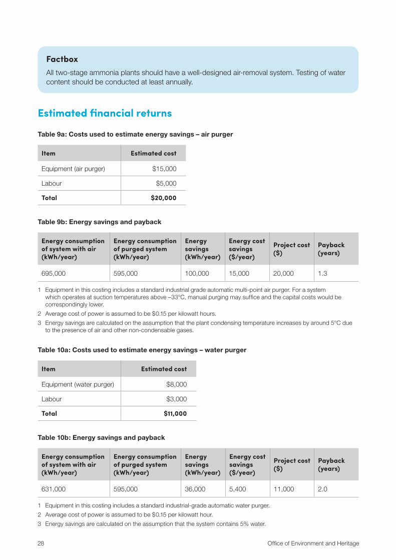
Estimated financial returns
Table 9a: Costs used to estimate energy savings – air purger
Item Estimated cost
Equipment (air purger) $15,000
Labour $5,000
Total $20,000
Table 9b: Energy savings and payback
Energy consumption of system with air (kWh/year)
Energy consumption of purged system (kWh/year)
Energy savings (kWh/year)
Energy cost savings ($/year)
Project cost ($)
Payback (years)
695,000 595,000 100,000 15,000 20,000 1.3
1 Equipment in this costing includes a standard industrial grade automatic multi-point air purger. For a system which operates at suction temperatures above –33°C, manual purging may suffice and the capital costs would be correspondingly lower.
2 Average cost of power is assumed to be $0.15 per kilowatt hours.
3 Energy savings are calculated on the assumption that the plant condensing temperature increases by around 5°C due to the presence of air and other non-condensable gases.
Table 10a: Costs used to estimate energy savings – water purger
Item Estimated cost
Equipment (water purger) $8,000
Labour $3,000
Total $11,000
Table 10b: Energy savings and payback
Energy consumption of system with air (kWh/year)
Energy consumption of purged system (kWh/year)
Energy savings (kWh/year)
Energy cost savings ($/year)
Project cost ($)
Payback (years)
631,000 595,000 36,000 5,400 11,000 2.0
1 Equipment in this costing includes a standard industrial-grade automatic water purger.
2 Average cost of power is assumed to be $0.15 per kilowatt hour.
3 Energy savings are calculated on the assumption that the system contains 5% water.
FactboxAll two-stage ammonia plants should have a well-designed air-removal system. Testing of water content should be conducted at least annually.

i am your industrial refrigeration guide 29
Technology 4: Heat recovery from discharge gas and oil cooling
Photo: Wat Als Photography/OEH
2% SIGNIFICANT HOT WATER GENERATION PLUS PLANT ENERGY SAVINGS OF UP TO
Overview y Principle: heat from compressor discharge gas and oil cooling is reclaimed for hot water
generation.
y Benefits: reduces energy consumption for hot water generation; reduces plant head pressure; achieves compressor power savings if the heat is recovered from low stage compressors.
y Savings: significant natural gas or LPG savings for hot water generation; up to 2% refrigeration plant energy savings.
y Ease of implementation: involves the installation of a hot water tank, de-superheating heat exchangers, oil cooling heat exchangers and pipework etc.

30 Office of Environment and Heritage
Energy used to heat water, whether it is electricity, gas or other fuel, can be reduced by using heat recovery to preheat water to between 50°C and 60°C. This provides a considerable saving in energy consumption.
FactboxOn screw compressors, the two main sources of heat rejection are the discharge gas and the cooling of compressor oil via an oil cooling process. On reciprocating compressors heat is rejected primarily via the discharge gas.
FactboxSubject to case-specific engineering studies, heat recovery is typically better suited to reciprocating compressors and natural refrigerants.
This technology can also be applied to liquid chillers, which are packaged units conventionally used to generate chilled water or a chilled mixture of glycol and water. They reject the heat generated by condensation to the environment via air-cooled condensers or cooling towers. The chiller units, in particular those using ammonia (R717) or carbon dioxide (R744) offer significant potential to recover otherwise wasted heat at useful temperature levels. Combined chiller and heat pump units are also available, which generate chilled fluid and hot water simultaneously by elevating the heat rejection temperature sufficiently to heat cold water to temperatures greater than 60°C.
On screw compressors, optimum heat recovery is achieved by installing:
y a common discharge gas de-superheating heat exchanger (de-superheater), either on the low-stage or high-stage discharge
y a secondary oil cooler in series with the existing oil cooler on each high-stage compressor.
The original oil cooler should be retained so the critical function of oil cooling is not compromised and is independent of hot water demand.
Extra oil cooling cannot be applied to reciprocating compressors.
Cold water is first passed through the de-superheater where it is pre-heated and then passed into the oil cooler where it is heated further to between 50°C and 60°C. This water is then stored in insulated hot water tanks and used as required. Typical applications for water in this temperature range include, but are not limited to:
y domestic hot water
y ‘washdown’ water for sanitisation purposes
y bottle warming or other process heating requirements
y pre-heated feedwater for a hot water generator supplying sterilisation and pasteurisation processes, where 80°C to 95°C water is required. By increasing the temperature of water entering a hot water generator, considerable energy savings are possible.
PrinciplesA facility that has refrigeration and hot water requirements can benefit by capturing heat that would otherwise have been rejected from the refrigeration plant. If left unexploited, these quantities of heat are rejected to the main heat rejection devices of the plant, i.e. the condensers.
i am your industrial refrigeration guide 31
The installation of a de-superheating heat exchanger to handle discharge gas results in a pressure drop on the refrigerant side that penalises plant energy consumption. However, a correctly engineered de-superheater decreases the load on the main condensers, allowing the system to run at head pressures low enough to offset the effect of the pressure drop caused by the heat exchanger. It may even provide a net improvement in compressor efficiency.
This can often be achieved simply by locating the pressure sensor used for variable head pressure control (see Technology 1) upstream of the de-superheater, rather than at the condensers.
Installing the de-superheater on the low stage discharge provides electrical (kilowatt hours) and gas (gigajoules) savings as follows:
y electrical (kilowatt hours) savings flow from the removal of some of the discharge gas superheat, which means less heat gets through to the high stage and therefore, reduced compressor and condenser power consumption.
y gas (gigajoules) savings flow from the heat recovery of the discharge gas superheat for water pre-heating.
Installation of de-superheater on the high stage gas discharge gives greater heat recovery effect and therefore greater gas savings. This is due to the greater heat rejection load and also the slightly elevated discharge temperature on the high stage than on the low stage. Power savings, however, are practically nil.
FactboxA site with relatively less demand for heat recovery and higher electrical tariffs (cost per kilowatt hour) is better suited to adopting a low-stage de-superheater. Conversely, a site with greater demand for heat recovery and lower electrical tariffs (cost per kilowatt hour) is better suited to adopting a high-stage de-superheater. Installation of de-superheaters on both the low stage and high stage provides greater overall savings, albeit at greater capital cost.
The heat recovery from process chillers is essentially like the recovery of heat from screw compressors or, in the case of reciprocating compressors, using a de-superheating heat exchanger only. Ammonia process chillers using reciprocating or screw compressors generally allow recovery of 10% to 20% of the total condensing heat in the form of useful heat. Where heat recovery is provided on hydrofluorocarbon (HFC) chillers, it is generally less feasible or commercially viable as discharge temperatures and the quality of recoverable heat is lower.
Plant benefits y Energy savings can be achieved due to reduced direct water heating. The savings could be
considerable on facilities using large amounts of hot water.
y Installing a de-superheating heat exchanger reduces the load on the main heat rejection devices of the plant, enabling the system to run at a slightly reduced head pressure. This can offset the effect of refrigerant pressure drop through the heat exchanger, if the equipment is selected carefully.
y Power savings can be achieved due to reduced high-stage compressor power consumption if a de-superheater heat exchanger is fitted to the low-stage discharge.

32 Office of Environment and Heritage
Achievable savingsHeat recoverable from the low-stage de-superheater and oil coolers of the screw compressors is around 16% of the low-stage load. If a high-stage de-superheater is used in place of a low-stage de-superheater, the heat recovery is around 20% of the low-stage load.
The achievable savings depend on:
y the plant having a continuous requirement for hot water such that discharge and oil cooling heat can be used continuously, as opposed to a plant requiring large quantities of water for a short period each day
y the load on the refrigeration system, as hot water production varies in direct proportion with this load
y the hot water storage capacity. A generous storage capacity increases savings at plants requiring large amounts of hot water
y the refrigerant used in the compressor/chiller. Ammonia or carbon dioxide units offer more heat recovery at higher temperatures than, for example, R134a units
y required water temperature.
Implementation
Information requirements
The minimum information you will need to implement a heat recovery system is:
y the number of compressors/chillers
y the make, model and type of each compressor/chiller (screw or reciprocating)
y the number of condensers
y the type of condenser (air-cooled, water-cooled or evaporative)
y hot water demand and required application temperature
y the current water heating equipment available space for equipment installation.
Equipment requirements
To recover heat from discharge gas and oil cooling you will need:
y A discharge gas de-superheating heat exchanger: a shell-and-tube type is good as it facilitates easy mechanical cleaning of the tubes. Refrigerant would be on the shell side and water on the tube side. Plate heat exchangers can also be used, but chemical cleaning may be required due to fouling over time. Plate heat exchangers are less expensive and require less installation space relative to shell-and-tube heat exchangers of similar capacity.
y An oil cooling heat exchanger: again, a shell-and-tube type is better, for the same reason as above. Oil would be on the shell side and water on the tube side.
y A three-way thermostatic valve on the oil return line: this will maintain the oil return temperature at a suitable level for normal operation of the compressor.
y Insulated hot water tanks: the size of the tanks should reflect hot water requirements, insulation and construction materials (typically stainless) and associated capital costs. If there is already a hot water tank on site a combination of a hot tank and a cold tank is a robust solution, where cold town water is fed into the cold tank as make-up and hot water to the application is drawn from the top of the hot water tank.

i am your industrial refrigeration guide 33
y A water circulation pump with variable speed drives (VSD) to circulate hot water between the tanks and the heat exchangers. The pump is controlled by a VSD based on the hot water temperature at the outlet of the oil cooler.
y Hot water circulation pumps to supply the application.
y Three-way mixing valves are optional and may be required to control the supply temperature to the application, especially in a facility which requires hot water at various temperatures.
Figures 10 and 11 illustrate two heat recovery arrangements:
Balance line Hot waterto field
High stagecompressor
Liquid to field
Suctionfrom field
Mains water
IntercoolerLow stage suctionaccumulator
Low stagecompressor
Low stagede-superheater
High stageoil cooler
Hot watertank
Cold watertank
Condenser
Liquid receiver
Figure 10: Schematic of heat recovery system with low-stage de-superheater
Balance lineHot water to field
High stagecompressor
Liquid to field
Suctionfrom field
Mains water
IntercoolerLow stage suctionaccumulator
Low stagecompressor
High stagedesuperheater
High stageoil cooler
Cold watertank
Condenser
Hot watertank
Liquid receiver
Figure 11: Schematic of heat recovery system with high-stage de-superheater
Note: These schematics are indicative of the concept. Industrial refrigeration systems usually contain multiple high-stage compressors such that the solution would involve a common discharge gas de-superheater and a new oil cooler for each high-stage compressor.

34 Office of Environment and Heritage
Estimated financial returns Capital costs to implement heat recovery depend on:
y the size of the de-superheater and oil coolers required
y the number of oil coolers required
y whether tanks are required
y the amount of pipework (ammonia, hot water) required.
Table 11: Parameters used to estimate energy savings from heat recovery
Parameter Value
Low-stage refrigeration load 500 kW
Low-stage suction temperature -35oC
Inter-stage temperature -2oC
Condensing temperature 35oC
Notes for Tables 11–13:
1 The equipment in these costings does not include hot water tanks or field (circuit) hot water pumps.
2 A single high-stage compressor has been assumed for estimating the costs and hence a single oil cooler has been indicated in the costing.
3 The usage profile as illustrated in Appendix B has been adopted for this analysis.
4 Average cost of power is assumed to be $0.15 per kilowatt hour.
5 Average cost of gas is assumed to be $10 per gigajoule.
The following estimated costs and savings are based on two heat-recovery scenarios:
Low-stage heat recovery
Table 12a: Costs used to estimate energy savings – low-stage de-superheater with oil cooler
Item Estimated cost
Equipment $10,000–$30,000
Labour $10,000–$20,000
Engineering $7,000
Programming $5,000
Total $32,000–$62,000
Table 12b: Energy savings and payback – low-stage de-superheater with oil cooler
Gas savings (GJ/year)
Gas cost savings ($/year)
Power savings (kWh/year)
Power cost savings ($/year)
Total cost savings ($/year)
Project cost ($) Payback (years)
1,670 16,700 23,000 3,450 20,150 32,000–62,000 1.6–3.1

i am your industrial refrigeration guide 35
High-stage heat recovery
Table 13a: Costs used to estimate energy savings – high-stage de-superheater with oil cooler
Item Estimated cost
Equipment $10,000–$30,000
Labour $10,000–$20,000
Engineering $7,000
Programming $5,000
Total $32,000–$62,000
Table 13b: Energy savings and payback – high-stage de-superheater with oil cooler
Gas savings (GJ/year)
Gas cost savings ($/year)
Power savings (kWh/year)
Power cost savings ($/year)
Total cost savings ($/year)
Project cost ($) Payback (years)
2,200 22,000 – – 22,000 32,000-62,000 1.5–2.8
Figure 12 indicates the variation in possible gas cost savings at different gas prices for this example of high-stage heat recovery.
0
$5,000
$10,000
$15,000
$20,000
$25,000
$30,000
$35,000
$40,000
1211109
Cos
t sav
ing
$/ye
ar
Gas cost $/Gigajoule (GJ)
Figure 12: Cost savings according to gas cost, using high-stage heat recovery

36 Office of Environment and Heritage
Case study: Rivalea AustraliaRivalea Australia, Corowa, implemented heat recovery from compressor discharge gas and oil cooling and reduced its LPG costs by $65,000 a year.
Table 14: Rivalea Australia energy savings and payback – heat recovery
LPG savings (GJ p.a.)
Energy cost savings ($p.a.)
Other cost savings (e.g. maintenance) ($p.a.)
Total cost savings ($p.a.)
Capital cost ($)
Payback period (years)
GHG savings (tonnes CO2 p.a.)
ESCs (number of certificates)
2,200 65,000 0 65,000 300,000 4.6 130 130
Rivalea Australia operates a large meat-processing facility in Corowa, New South Wales, and had an annual LPG consumption of approximately 50,000 gigajoule in the past, which cost over $1 million each year. The LPG was mainly consumed by a large boiler for steam and hot water generation. Hot water was used for wash-down, clean-in-place and other purposes.
In 2012 Rivalea identified a significant LPG saving opportunity – to recover the heat from the refrigeration plant on site for hot water generation.
The project involved:
y installing a high-stage de-superheating heat exchanger on the common discharge line of the refrigeration plant
y installing heat recovery oil coolers onto two high-stage screw compressors which operate for most of the time
y installing a hot water tank for hot water storage, along with all the associated pipework to connect the tank.
The system employs two stages of heat recovery: first the water is fed through the discharge gas heat de-superheating heat exchanger, then it is fed through the oil coolers for further heating.
The heat recovery achieves a hot water temperature of 70°C. Annual energy savings are 2200 gigajoule (4.4% of annual site gas use) due to the reduction in LPG required. This corresponds to a financial saving of $65,000 a year.
The heat recovery system has played a stabilising role in our hot water system, reducing our overall consumption of LPG in a challenging production environment. The infrastructure and instrumentation installed has allowed us to closely monitor our hot water production and plan future additional heat recovery options from other sources.
Ian Longfield, Rivalea Senior Environmental Officer

i am your industrial refrigeration guide 37
Figure 13: Rivalea Australia’s heat recovery system: A. de-superheating heat exchanger, B. heat recovery oil cooler, and C. hot water storage tankPhotos: Rivalea Australia/OEH

38 Office of Environment and Heritage
Technology 5: Variable defrost timing and termination
3% PLANT ENERGY SAVINGS OF UP TO
Overview y Principle: evaporator defrost timing and termination are optimised to prevent excess heat
entering the refrigeration area.
y Benefits: reduces plant energy consumption and defrost energy consumption; stabilises refrigeration plant operation.
y Savings: typical plant energy savings can be up to 3%.
y Ease of implementation: involves installing temperature sensing equipment and cool room load tracking devices, and programming the control system.
Photo: Wat Als Photography/OEH
i am your industrial refrigeration guide 39
Principles
FactboxMost facilities have cool rooms or freezer rooms that use fan coil evaporator units. Over time, ice forms on these coils and in their condensate trays due to airborne moisture. The rate at which ice is formed on a coil depends on several factors such as room temperature, cooling load, ambient conditions and number of door openings. As the ice layer on the coils increases, the coil’s heat exchanging capacity decreases. Hence, there is a need to defrost coils.
FactboxConventional defrosting methods use either hot gas, electricity, air or water. Many ammonia plants use hot gas defrost as there is sufficient heat available from the refrigeration plant and it is cheaper than electricity.
The process of defrosting introduces heat into the refrigerated space, increasing the plant’s workload and energy consumption. The defrosting process also consumes energy. If defrosting methods are not optimised, refrigeration plant efficiency suffers.
‘Variable defrost timing and termination’ refers to managing the interval between defrosts, the duration of the defrosting process and termination of defrosts. By convention, the frequency and duration of defrosts are fixed, regardless of room temperature and work load between defrosts. If there are too many defrosts or they last too long, heat will be needlessly added to the room. Hence optimised defrost management reduces overall refrigeration plant energy consumption.
The variable defrost timing and termination proposed involves monitoring the time over which the coil has been operating at full capacity. The interval between defrosts will be shorter if the coil has been running continuously at full capacity and longer if it has been running at lower capacity. The capacity of the coil can be found by assessing the amount of cooling supplied to it over a period. In the case of a flooded ammonia evaporator coil, the capacity is the time for which the liquid solenoid valve is open.
Plant benefits y Managed defrosting intervals prevents wasteful defrosting during low-load periods.
y Optimised defrost duration and termination of defrost prevents excess heat entering the cool room, easing the load on the refrigeration system and preventing energy waste.
y Quick termination of defrost by electric defrosting units also saves unnecessary power consumption by the electric heaters.
y Reduced need for defrosting during low-load situations means the refrigeration plant will be stable for longer periods of time. Similarly, with an ammonia evaporator coil, fewer defrosts means fewer suction pressure fluctuations, leading to more stable operation.

40 Office of Environment and Heritage
Achievable savingsAchievable annual savings depend on:
y the number, type and size of fan coil units in the room
y the room temperature
y the cooling load profile
y the type of defrost: hot gas, electric, air or water
y the number of defrosts and the defrost interval currently employed
y the defrost relief point: low temperature, intercooler or economiser vessel (see Technology 9, 3: Defrost relief piping to intercooler or economiser).
Figure 14 illustrates the effect of employing fixed defrost intervals and durations. As the average freezer load reduces, there is an unnecessary penalty on the refrigeration plant that can be avoided by employing a defrost management system.
Ener
gy e
�ci
ency
pen
alty
(%
)
0
1
2
3
4
Freezer load (%)
100755020
Figure 14: Energy penalty associated with conventional defrosts

i am your industrial refrigeration guide 41
Implementation
Information requirements
You need to know the:
y make and model of fan coil units in each of the rooms
y defrost technique applied
y coil arrangement within plant and circuit design
y room temperature.
Equipment requirements
To facilitate a sound defrost management strategy you will need:
y A temperature sensing device attached to the face of the evaporator coil. When coil temperature reaches 10°C, the defrost is complete and can be terminated.
y A means of tracking the room cooling load, such as a monitoring solenoid or control valve.
y A high-level PLC (or remote control management system (CMS) unit) which controls the defrost system.
Estimated financial returnsThis project is mainly achieved by implementing control algorithms. The only equipment required is a coil temperature thermostat or sensor to terminate the defrost cycle. The estimated cost of equipment and initial definition of the control algorithm is approximately $1500 per evaporator, if the site has a control system to which the thermostat can be connected. Optimisation costs would be additional based on the level of optimisation required.
For a site with 10 evaporators, each of 50 kilowatt capacity, typical capital costs and payback could be:
Table 15: Energy savings and payback
Energy savings (kWh/year)
Energy cost savings ($/year)
Project cost ($)
Payback (years)
100,000 15,000 15,000 1.0

42 Office of Environment and Heritage
Technology 6: Variable cold store temperatures
Photo: Wat Als Photography/OEH
2% PLANT ENERGY SAVINGS OF UP TO
Overview y Principle: a higher cold store temperature is set during the day to enhance system
efficiency and reduce peak power.
y Benefits: saves energy, saves energy cost and reduces peak demand.
y Savings: typical plant energy savings can be up to 2%, plus cost savings and peak demand saving.
y Ease of implementation: involves reprogramming the cold store control system and the application of phase change materials if required.
i am your industrial refrigeration guide 43
Principles
FactboxCold stores generally run to a fixed set-point room temperature throughout the day and night. This causes the refrigeration plant load to increase during peak periods to maintain temperature, and to run largely unloaded during off-peak periods.
Factbox The main sources of heat in a cold store are transmission and infiltration loads, introduced via walls, the floor and roof, which allow heat and outside ambient air into the cold store. Heat also enters when doors are opened. This means plant load is higher during the day when energy charges are higher and lower at night.
For products that require cold storage and can tolerate slight variations in storage temperature, such as meat products and frozen vegetables, variable cold store temperatures can exploit off-peak efficiencies and lower off-peak power costs, and minimise peak demand costs.
The workload of the refrigeration plant, and its energy consumption, can be reduced during the day by allowing temperatures to rise slightly. The plant can then cycle down to a lower temperature at night, when it is cheaper to achieve lower temperatures. For example, a cold store usually running at –20oC can be reduced to –22oC at night and run at –18oC for part of the day.
This variable temperature control strategy involves reducing temperatures during off-peak periods and raising them during the day. This shifts the load on the plant by running a higher suction pressure during off-peak hours, thus possibly reducing overall energy consumption and costs and avoiding demand peaks.
Plant benefitsBenefits include:
y possible daytime energy savings by allowing higher cold store temperatures
y possible overall reduction in energy costs
y possible reduction in peak demand costs due to intelligent load shifting.
The benefits will vary depending on the specific facility and the variation allowed by the products in the cool room. Energy consumption may slightly increase due to the higher workload at night, but energy costs and peak demand costs may reduce, hence modelling should be conducted based on specific operating conditions.

44 Office of Environment and Heritage
Achievable savingsAchievable annual savings depend on:
y the amount of temperature variation allowed by the products
y the extent to which suction pressures can be varied
y peak and off-peak energy costs (cost per kilowatt hour) and peak demand costs (cost per kilo volt-ampere)
y whether the refrigeration system is dedicated to the cold stores or runs other production loads. If the system runs other loads at lower temperatures, such as a blast freezer, no benefit may be possible unless the suction to the cold stores is split: see Technology 9.
ImplementationThis project involves programming suitable control logic to allow the cool room temperature and plant suction set-points to switch between peak and off-peak periods.
Estimated financial returnsThis project is mainly achieved by implementing control algorithms. The estimated cost of initial definition of the control algorithm would typically be between $5000 and $10,000 depending on the size of the installation, and assuming a modern programmable logic controller (PLC) is already in operation on the site. Optimisation costs would be additional based on the level of optimisation required.
Factbox: Phase change materialsThis strategy treats goods inside cold stores as a medium for storage of cooling, which is restricted by the properties of the goods – some goods do not allow large variation of the temperature so only a small amount of cooling can be stored. A modern solution to this is the application of phase change materials (PCMs), which can absorb or release significant cooling with only a slight change of their temperature.
PCMs release large amounts of thermal energy upon freezing in the form of latent heat and absorb equal amounts of energy from the immediate environment upon melting. This enables the cooling to be stored in an off-peak period and used at a later peak period without causing large variation of the room temperature.
The simplest and most effective phase change material is water/ice, although its freezing point of 0°C precludes it from most energy storage applications. Several other PCMs have been developed and introduced into the market – they can freeze and melt like water/ice but at temperatures from the cryogenic range to several hundred degrees Celsius. For different applications, different types and portions of the PCM solutions need to be considered.
Figure 15 shows some typical PCM products that are on the market. PCM solutions are encapsulated in sealed containers, commonly with a rectangular or tube shape. Containers can be installed as part of the cold store fabric, for example, hanging in the ceiling space (see figure 16) or they can be placed on pallets and stored with the shelves. They can also be stacked in tanks to chill the secondary fluid in the system, e.g. glycol or water, in which the tank acts as a heat exchanger. Figure 17 shows the schematics of a typical system.

i am your industrial refrigeration guide 45
Figure 15: phase change materials (PCM) encapsulated in sealed rectangular (A) and tube (B) containers
Figure 16: PCMs installed in the ceiling space Photos: OEH
Phase change materials

46 Office of Environment and Heritage
Figure 17: Schematic of PCMs in a typical tank operation during (A) charging and (B) discharging
TES tank
Optional by-pass
Optional by-pass
Optional by-pass
3-wayvalve
3-wayvalve
3-wayvalve
2-wayvalve
2-wayvalve
Chokevalve
Tankpump
Maincirculation
pump
Pressurereducing
valve
Chiller
Load
Phase change materials
Load
Optional by-pass
Optional by-pass
Optional by-pass
3-wayvalve
3-wayvalve
3-wayvalve
2-wayvalve
2-wayvalve
Chokevalve
Tankpump
Maincirculation
pump
Pressurereducing
valve
Chiller
TES tank

i am your industrial refrigeration guide 47
Technology 7: Variable evaporator fan speeds
Photo: Wat Als Photography/OEH
2% PLANT ENERGY SAVINGS OF UP TO
Overview y Principle: the speed of evaporator fans is controlled to reduce fan power and excess heat
entering the refrigerated space.
y Benefits: reduces evaporator power and plant energy consumption; stabilises cool room temperature.
y Savings: typical plant energy savings can be up to 2%.
y Ease of implementation: involves installing variable speed drives (VSD) on evaporator fans and implementing fan speed control logic.

48 Office of Environment and Heritage
PrinciplesFan-coil evaporators are used in most industrial cold storage applications. These evaporator fans are rarely speed controlled, running at full speed and turning on and off as required. The evaporator fan motor is a continuous heat load on the cool room which in turn, is an additional load on the refrigeration plant.
FactboxThe evaporator fan is a major part of the overall cooling load on a cold space, especially in off-peak periods. They tend to be run unnecessarily at full speed, even when workload is low. By varying the fan speeds to suit load, energy savings are possible because lower fan speed translates to less heat being introduced to the cool room.
FactboxIn applications using multiple evaporators, this operation is best achieved by simultaneously varying the speed of all evaporator fans to suit the load, to ensure uniform air distribution in the cold store.
Reduction in fan speed is directly proportional to evaporator capacity. However, a fan’s power consumption is proportional to the cube of its speed. Therefore, reducing fan speed by 20% reduces fan power consumption by approximately 50%. Hence considerable energy savings are achievable using variable evaporator fan speeds.
Note: The concept of variable evaporator fan speed control is not necessarily applicable to blast freezing as evaporator fans may need to run at full air flow to achieve full freezer performance.
Plant benefits y Variable speed operation provides good control of room temperature at low load compared to on/
off fan cycling.
y A considerable reduction in fan power by slight reduction in fan speed.
y A reduced load in the cold store due to reduced heat introduced into the rooms by the slower running fans.
Achievable savings Figure 18 illustrates the power savings with respect to room load due to installing variable speed drives on evaporator fans. As the graph indicates, the savings are greatest at low room loads. The horizontal line between loads of 10% and 50% indicates that a minimum fan speed of 50% has been considered in the modelling, which is typical for most evaporator fans.

i am your industrial refrigeration guide 49
0
10
20
30
40
50
60
70
80
90
100
100908070605040302010
Tota
l fan
pow
er s
aved
(%)
Room load (%)
Figure 18: Fan power savings with room load
Achievable annual savings depend on:
y the load profile
y the size and number of evaporator fans (kW)
y the number of cold stores in the facility.
ImplementationYou will need:
y Variable speed drives for the evaporator fans – typically one VSD per evaporator. The VSD would control all fans in the evaporator unit and needs to be selected for the maximum current that could be drawn when all fans run at full speed.
y Sufficient programming capability in the control system to facilitate effective speed control logic.
Estimated financial returnsCapital costs to implement variable evaporator fan speeds depend on:
y the number of evaporators in the facility
y the size of the evaporator fan motors.
For a cold store with a total evaporator capacity of 500 kilowatts (10 x 50 kilowatt units), typical capital costs could be:

50 Office of Environment and Heritage
Table 16a: Costs used to estimate energy savings
Item Estimated cost
Equipment $20,000–$50,000
Labour $15,000–$50,000
Engineering $5,000
Programming $8,000
Total $48,000–$113,000
Table 16b: Energy savings and payback
Energy consumption of conventional system (kWh/year)
Energy consumption of improved system (kWh/year)
Energy savings (kWh/year)
Energy cost savings ($/year)
project cost ($)
payback (years)
370,000 80,000 290,000 43,500 48,000–113,000 1.1–2.6
1 Equipment in this costing includes 10 variable speed drives (4 kilowatts each), shielded cabling, electrical wiring and enclosures for VSDs.
2 The usage profile as illustrated in Appendix B has been considered for this analysis.
3 Average cost of power is assumed to be $0.15 per kilowatt hour.
Case study: Montague Cold StorageMontague Cold Storage, Tullamarine, implemented variable evaporator fan speed control logic and reduced its evaporator electricity costs by 40%, equivalent to $18,000 a year.
Table 17: Montague Cold Storage energy savings and payback
Electricity savings (MWh p.a.)
Energy cost savings ($p.a.)
Other cost savings (e.g. maintenance) ($p.a.)
Total cost savings ($p.a.)
Capital cost ($)
Payback period (years)
GHG savings (tonnes CO2 p.a.)
ESCs (number of certificates)
200 18,000 0 18,000 70,000 3.8 192 212
Montague Cold Storage is a family-owned cold-storage business that established its first facility in 1948. It now operates temperature-controlled storage and inventory management facilities at six sites throughout Victoria, and one in Tasmania.
Its facility at Tullamarine, Victoria, offers various freezer and chiller rooms in two buildings. Cooling is provided by a common ammonia refrigeration system with fan coil evaporators installed in the rooms, as shown in figure 19.
Before the project, all evaporator fans at the site operated at fixed speed, except in the loading area in the south building. The fans were cycled on and off to keep the rooms within an operating temperature range, but the overall fan energy was often needlessly high.
Montague Cold Storage realised this was an opportunity for improving plant efficiency. The company installed 19 VSDs on its evaporator fans and implemented smart control logic. The fans now operate at an optimum speed, based on actual room temperature.
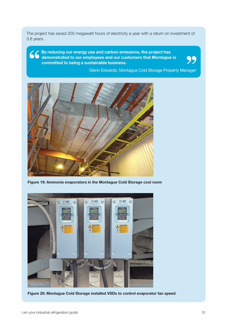
i am your industrial refrigeration guide 51
The project has saved 200 megawatt hours of electricity a year with a return on investment of 3.8 years.
By reducing our energy use and carbon emissions, the project has demonstrated to our employees and our customers that Montague is committed to being a sustainable business.
Glenn Edwards, Montague Cold Storage Property Manager
Figure 19: Ammonia evaporators in the Montague Cold Storage cool room
Figure 20: Montague Cold Storage installed VSDs to control evaporator fan speed
Photo: OEH
Photo: OEH
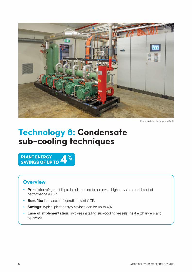
52 Office of Environment and Heritage
Technology 8: Condensate sub-cooling techniques
Photo: Wat Als Photography/OEH
4% PLANT ENERGY SAVINGS OF UP TO
Overview y Principle: refrigerant liquid is sub-cooled to achieve a higher system coefficient of
performance (COP).
y Benefits: increases refrigeration plant COP.
y Savings: typical plant energy savings can be up to 4%.
y Ease of implementation: involves installing sub-cooling vessels, heat exchangers and pipework.

i am your industrial refrigeration guide 53
Refrigerant that has condensed in the condensers of a refrigeration plant is commonly stored in liquid receivers and supplied to either the field (circuit) as high-pressure liquid or the low-pressure vessels of the plant. In most cases, the liquid is either at saturation temperature or only slightly sub-cooled. Further sub-cooling of the liquid improves the thermodynamics of the refrigeration plant, permitting energy savings due to reduced flash gas and therefore achieving a higher COP.
This further sub-cooling can be achieved in different ways; two methods are considered here:
1. sub-cooling using cold town water supply to the condensers
2. sub-cooling using economisers on high-stage screw compressors.
FactboxThese two methods can be used separately and, in some cases, may be feasible in combination. Where only reciprocating compressors are used, town water sub-cooling is the only option. The more modern (and positive) trend towards using rainwater storage may render this option less feasible, as water from rainwater tanks tends to be warmer than town water.
1. Condensate sub-cooling with town water supplyPrinciplesOn a system using cooling towers or evaporative condensers, sub-cooling of high pressure refrigerant liquid can be achieved by exchanging heat from the condensate with incoming town water used as make-up water. The incoming town water is generally between 10°C and 15°C depending on the time of the year and the geographical location. Elevating the temperature of incoming town water before it enters the cooling towers or evaporative condensers has a marginal effect on their performance. Thus, the relatively cold town water can be used to maximise efficiency by first passing it through a condensate sub-cooler, then routing it to the cooling towers or evaporative condensers. This sub-cooler is typically a refrigerant-to-water plate heat exchanger or a water jacket sub-cooling arrangement around the refrigerant liquid supply line from the liquid receiver.
Plant benefitsThis technology increases the COP of the refrigeration plant without impacting maintenance costs or plant operation.
Achievable savings Achievable annual savings depend on:
y town water supply temperature
y the condensing (liquid) temperature of the plant.

54 Office of Environment and Heritage
0
1
2
3
4
5
6
201510
CO
P im
prov
emen
t (%
)
Town water temperature: (°C)
25̊ 30̊ 35̊20̊
Figure 21: COP improvement due to condensate sub-cooling by town water
Figure 21 illustrates the improvement in efficiency of the system due to condensate sub-cooling by town water. As the town water temperature increases, the COP improvement reduces. Similarly, as condensing temperature decreases for given water inlet temperature, the COP improvement reduces. Variation in town water temperature is mainly due to geographical and seasonal variations.
Implementation
Information requirements
You need to know the:
y make and model details of compressors, cooling towers and evaporative condensers
y size (diameter) of the main high-pressure refrigerant liquid line.
Equipment requirements
You will need:
y A refrigerant-to-water plate heat exchanger. Alternatively, a tube-in-tube section could be installed on the liquid supply line from the liquid receiver assuming the required straight line length is available.
y Insulation for the sub-cooled refrigerant liquid line if the pipe length of the sub-cooled line is considerable.

i am your industrial refrigeration guide 55
Estimated financial returns
Capital costs to implement condensate sub-cooling depend on:
y the size of heat exchanger required depending on refrigerant flow
y the type of heat exchanger – plate or tube-in-tube.
For a refrigeration system with a peak heat rejection load of 500 kilowatt, typical capital costs could be:
Table 18a: Costs used to estimate energy savings
Item Estimated cost
Equipment $3,000
Labour $4,000
Engineering $2,000
Total $9,000
Table 18b: Energy savings and payback
Energy consumption of conventional system (kWh/year)
Energy consumption of improved system (kWh/year)
Energy savings (kWh/year)
Energy cost savings ($/year)
Project cost ($)
Payback (years)
502,000 487,000 15,000 2,250 9,000 4.0
1 The annual energy savings are calculated based on an average water temperature of 12°C and average condensing temperature of 30°C.
2 The usage profile presented in Appendix B has been used for this analysis.
3 Equipment in this costing includes a plate heat exchanger and refrigerant and cooling water pipework.
4 Average cost of power is assumed to be $0.15 per kilowatt hour.

56 Office of Environment and Heritage
2. Condensate sub-cooling with economisersPrinciplesOn any single or two-stage ammonia plant containing screw compressors on the high side, condensate can be sub-cooled by the refrigerating effect of the so-called economiser port of these compressors.
FactboxThe economiser port provides a suction pressure which falls between that of main suction pressure of the high-stage compressor and the discharge pressure (system condensing pressure in this case). For most typical high-stage applications, the intermediate suction pressure is typically equivalent to evaporation temperatures in the range of 0°C to 10°C.
FactboxThis concept is different from condensate sub-cooling by town water in that the refrigerant liquid can be sub-cooled down to low temperatures by the economiser effect even during summer conditions, when town water temperatures can be elevated. With a refrigerant sub-cooling heat exchanger using town water, the minimum refrigerant outlet temperature would be around 15oC (or higher depending on the temperature of the water coming in) whereas the minimum refrigerant outlet temperature on an economiser system would be around 8oC to 10oC (on a system with a high-stage suction temperature of –10oC).
By expanding some of the high-pressure liquid refrigerant from the liquid receiver to this intermediate suction pressure, the cooling effect of the evaporating refrigerant at this pressure can be used to sub-cool the remaining high pressure liquid refrigerant to a lower temperature before it is then expanded to the intercooler or high-stage suction pressure, thus reducing the amount of flash gas developed in the intercooler or at high-stage suction pressure. Typically, this cooling effect is used in several different ways:
y open flash economiser vessel, in which all refrigerant is first expanded into the economiser, and then expanded further into the intercooler/high-stage suction vessel
y economiser vessel with flooded sub-cooler coil, in which the remaining high-pressure refrigerant is sub-cooled by immersion within the evaporating refrigerant at intercooler pressure
y sub-cooler plate heat exchanger, in which the remaining high-pressure refrigerant is sub-cooled by evaporating refrigerant within the heat exchanger. Several different arrangements are possible.
Energy savings are achieved due to the reduced flash gas introduced into the intercooler vessel and hence increased refrigeration plant efficiency.
FactboxThis concept could be beneficial on sites that use recovered rainwater as feed water to the evaporative condensers, as this reduces or eliminates the capability to sub-cool the refrigerant liquid. On some sites, a combination of the two technologies could yield significant energy savings, although at a high capital cost. For example, the system could benefit from low town water temperatures in winter, and then largely rely on economiser operation in summer, with a combination of modes during other seasons.

i am your industrial refrigeration guide 57
Plant benefitsThis technology increases the COP of the refrigeration plant without impacting maintenance costs or plant operation.
Achievable savings Achievable annual savings depend on inter-stage and/or high-stage suction and the condensing and high-pressure liquid temperatures of the plant, which have an impact on the intermediate pressure at which the economiser vessel operates. This finally governs the temperature to which the refrigerant liquid can be sub-cooled.
Figure 22 illustrates the improvement in the COP of the system and figure 23 illustrates the increase in available capacity of the system due to condensate sub-cooling using an economiser vessel on the high-stage compressors, for a range of suction temperatures (Ts) of the system. This is the suction temperature of single-stage systems (dairies, breweries, wineries) or the interstage temperature of two-stage systems (abattoirs, cold stores, chicken processers, etc.). The lower this suction temperature, the greater is the increase in COP. For a typical system with a suction temperature of -10oC and a condensing temperature of 35oC, the increase in COP is around 4.5% and the increase in refrigeration capacity is around 7%.
5040302010
CO
P in
crea
se (%
)
0
1
2
3
4
5
6
7
8
9
10
Condensing temperature Tc (°C)
Ts= -20̊ Ts= -15̊ Ts= -10̊ Ts= -5̊Ts= -25̊
Figure 22: COP improvement due to condensate sub-cooling by high-stage economiser

58 Office of Environment and Heritage
5040302010
Cap
acity
incr
ease
(%)
0
14
12
10
8
6
4
2
Condensing temperature Tc (°C)
Ts= -20̊ Ts= -15̊ Ts= -10̊ Ts= -5̊Ts= -25̊
Figure 23: Increase in capacity due to condensate sub-cooling by high-stage economiser
Implementation
Equipment requirements
You will need:
y either of the above equipment combinations, such as:
y an open flash economiser vessel able to service some or all the high-stage compressors in the plant
y an economiser vessel fitted with a liquid sub-cooling coil
y a liquid sub-cooling plate heat exchanger operated either in flooded or direct expansion mode
y insulation for the sub-cooled refrigerant liquid line if it is long.
Estimated financial returnsCapital costs to implement this opportunity depend on:
y the size of economiser vessel or heat exchanger required
y the number of high-stage compressors to be economised.
For a refrigeration system with a high-stage load of 500 kilowatts, capital costs could be:

i am your industrial refrigeration guide 59
Table 19a: Costs used to estimate energy savings
Item Estimated cost
Equipment $8,000
Labour $6,000
Engineering $5,000
Total $19,000
Table 19b: Energy savings and payback
Energy consumption of conventional system (kWh/year)
Energy consumption of improved system (kWh/year)
Energy savings (kWh/year)
Energy cost savings ($/year)
Project cost ($)
Payback (years)
586,000 558,000 28,000 4,200 19,000 4.5
1 The usage profile presented in Appendix B has been used for this analysis.
2 Equipment in this costing includes a vertical economiser vessel, pipework, fittings and insulation.
3 Average cost of power is assumed to be $0.15 per kilowatt hour.
Case study: Rivalea AustraliaRivalea Australia, Corowa, implemented condensate sub-cooling with an economiser in its refrigeration plant and reduced its electricity costs by $33,000 a year.
Table 20: Rivalea Australia energy savings and payback – condensate sub-cooling
Electricity savings (MWh p.a.)
Energy cost savings ($p.a.)
Other cost savings (e.g. maintenance) ($p.a.)
Total cost savings ($p.a.)
Capital cost ($)
Payback period (years)
GHG savings (tonnes CO2 p.a.)
ESCs (number of certificates)
190 33,000 0 33,000 130,000 3.9 182 294
Rivalea’s Corowa facility has a two-stage ammonia system and features a high-stage screw compressor. It was possible to improve the system COP by sub-cooling the refrigerant condensate using an economiser.
An economiser vessel set was installed (figure 24), which includes a vertical vessel, an oil drain pot, a flooded plate heat exchanger, a liquid feed electronic expansion valve and other valves and instruments.
Part of the high-pressure liquid from the liquid receiver is fed into the economiser vessel which operates at 6°C. The rest of the high-pressure liquid is sub-cooled from 30°C to around 11°C in the plate heat exchanger. The evaporated vapour in the vessel returns to the high-stage compressors.
This project has reduced refrigeration energy consumption by 8% and saved $33,000 a year in electricity costs.

60 Office of Environment and Heritage
Figure 24: Rivalea’s economiser vessel set for condensate sub-cooling
Case study: Rivalea Australia
Refrigeration is one of the major electrical energy loads in our plant, so even small efficiencies can make a large difference to the overall running costs. Sub-cooling the condensate made a lot of sense and has operated trouble-free since installation. Power consumption at the plant has reduced and this project has contributed to the savings.
Ian Longfield, Rivalea Senior Environmental Officer
Photo: Riverlea/OEH
Economiser vessel set

i am your industrial refrigeration guide 61
Technology 9: Ammonia plant process design review
Photo: Wat Als Photography/OEH
10% PLANT ENERGY SAVINGS OF UP TO
Overview y Principle: deficiencies in plant design and installation are identified and addressed through
a thorough review of plant efficiency.
y Benefits: optimises plant pressures and improves efficiency.
y Savings: typical plant energy savings can be up to 10%.
y Ease of implementation: depends on the type of the design and installation deficiencies.

62 Office of Environment and Heritage
Many plants may be inefficient due to poor design and installation. A thorough review of refrigeration plant can identify shortcomings or bottlenecks that are reducing plant efficiency.
These can include:
y undersized or poorly located heat exchangers
y fouling of heat exchanger surfaces due to corrosion, ice formation, oil accumulation or other causes
y undersized suction or discharge lines or associated line components resulting in excessive pressure losses
y incorrect routing of suction lines, in particular wet return lines, resulting in excessive pressure drop, excessive liquid retention or unstable flow.
FactboxA design review can also address other issues such as:
y having a combination of loads requiring different evaporation temperatures from a single suction pressure level, with the aim of splitting suction pressure levels. This typically occurs where blast freezing and cold storage, or air conditioning and process room cooling co-exist
y adjusting the set levels of operating suction pressures in the plant, with the view to raising compressor suction pressure
y employing a defrost relief strategy to the highest possible suction pressure level in the plant
y eliminating liquid injection oil cooling in preference to thermosyphon or water cooling on screw compressors.
For most plants, poor design can reduce plant efficiency by introducing pressure or temperature losses in the system (see figures 25, 26 and 27).
1. Removing bottlenecks PrinciplesBottlenecks can occur in items such as heat exchangers, suction lines or other devices with a design flaw – due to their configuration or condition – which leads to running the refrigeration plant inefficiently.
The identification of bottlenecks requires careful review of the plant design documentation, process diagrams, arrangement drawings and operating manuals, in conjunction with a plant inspection by a competent engineer.
The effect of suction temperature on the efficiency of two-stage and single-stage refrigeration plants is illustrated in figures 25 and 26. The effect of a pressure drop in the discharge line on the efficiency of a refrigeration plant is illustrated in figure 27 (see Appendix B for more details).

i am your industrial refrigeration guide 63
0
2
4
6
8
10
12
14
16
18
20
-30-32-34-36-38-40
Incr
ease
in C
OP
(%)
Suction temperature (°C)
Figure 25: Effect of suction temperature on the COP of a two-stage plant
0
2
4
6
8
10
12
14
16
18
20
Incr
ease
in C
OP
(%)
Suction temperature (°C)
-15 -14 -13 -12 -11 -10
Figure 26: Effect of suction temperature on the COP of a single-stage plant

64 Office of Environment and Heritage
200100500
Incr
ease
in C
OP
(%)
0
2
4
6
8
10
12
14
16
18
Reduction on discharge line pressure drop kilopascal (kPa)
30̊ C Cond temp 35̊ C Cond temp25̊ C Cond temp
Figure 27: Effect of discharge pressure drop on the COP of a refrigeration plant
Plant benefitsBenefits of removing bottlenecks can include:
y higher suction and/or lower discharge pressures which reduce compressor power consumption, for a given cooling capacity
y floating or optimised inter-stage pressures allowing the total power consumption of all compressors to be minimised
y maximising the operating suction pressures (low suction or inter-stage), which will maximise the availability of the plant and could result in capital cost savings by avoiding or reducing additional compressor capacity requirements where plant capacity needs to be extended.
Achievable savingsAchievable annual savings depend on:
y the original design and current age of heat exchangers
y the current suction and discharge line design and routing.
ImplementationOnce they have been identified and their effect on the plant established, removing bottlenecks generally requires the operator to:
y replace or relocate undersized or poorly located heat exchangers
y address the causes of fouling or replace corroded heat exchangers where fouling has been identified

i am your industrial refrigeration guide 65
y replace suction or discharge lines or line components that are undersized
y rectify incorrect line routing.
Often, when bottlenecks have been removed, suction pressures can be raised or controlled at variable levels, where previously they had to be kept low to achieve plant performance.
Estimated financial returnsThe capital costs vary depending on the specific bottleneck being addressed such as:
y cleaning or replacing heat exchangers
y replacing suction and/or discharge lines, depending on sizing and extent of replacement required.
Due to the various types of upgrades that might be required, it is not possible to give an overall indication of financial returns. See Appendix B for potential savings.
2. Suction splittingPrincipleFacilities that require blast freezing usually also have holding freezers to store frozen product. Often, the blast freezers and holding freezers are operated from the same suction vessel. The inherent inefficiency in this approach is that the higher temperature in a cold storage plant (typically at –30°C suction) is generated at an excessively low temperature designed for blast freezing (typically at –40°C). Furthermore, and as indicated in figures 25 and 26, raising suction temperatures where possible will improve refrigeration plant efficiency.
FactboxA similar situation exists in facilities that have cool rooms or process areas at intermediate temperatures (0°C to 10°C) and comfort air conditioned loads (18°C to 25°C) both connected to the intermediate suction temperature (typically –10°C).
Plant benefitsBenefits of suction splitting include:
y energy savings due to running holding freezers at appropriate suction temperature rather than at blast freezer suction – this allows suction temperature to be elevated by about 15°C
y in plants where compressor duty is near design capacity, splitting the suction relieves compressor capacity so that throughput in the blast freezers can be increased if required, assuming suction lines are adequately sized
y energy savings and suction splitting as above, but at medium temperature levels.

66 Office of Environment and Heritage
Achievable savingsFigure 26 illustrates the effect of suction splitting on the efficiency of the plant, which contains blast freezers and holding freezers, for various holding freezer suction temperatures. The efficiency improvement is in the range of 13% to 16% for the range of suction temperatures mentioned above.
Achievable annual savings depend on:
y the actual difference in temperature between the two suction levels required – the greater the difference in temperatures, the greater the savings
y the load profile
y the number of days of production – the greater the number of days, the larger the savings.
See Appendix B for potential savings.
ImplementationSuction splitting on low temperatures involves separating the suction of the blast freezers and the holding freezers by introducing a new suction level in the plant to independently serve the holding freezers. This involves raising the suction temperature for the holding freezer, thus improving refrigeration plant efficiency.
Suction splitting on medium temperatures may involve diverting the high temperature (18°C to 25°C) loads to a separate suction level. In plants with economised screw compressors, this can be achieved by using a side load connection, which handles dual suction pressures without the need to dedicate separate compressors to both applications.
Various technical solutions as described below are possible for a project of this nature. The costs could vary widely based on the solution chosen and therefore have not been estimated.
Low cost solution
Use existing equipment if available:
y Assume the plant has an existing pressure vessel that could be used for the new suction temperature level.
y On systems with blast freezers and holding freezers, use existing low temperature liquid pumps to feed liquid from the low temperature vessel to the holding freezer. This would lead to a slight reduction in energy savings as compared to using dedicated liquid pumps.
y Assume the plant has a compressor that can be dedicated to serve the new suction temperature level.
Medium cost solution
If there is no dedicated pressure vessel available in the plant:
y A simple ‘slop pot’ solution could work where the wet return vapour from the freezer evaporators could be directed, and the dry suction gas provided, to the respective compressors. This is a less expensive solution than a full-scale pressure vessel.
y Use existing low-temperature liquid pumps to feed liquid from the low-temperature vessel to the holding freezer. This would lead to a slight reduction in energy savings as compared to using dedicated liquid pumps.
y Assume the plant has a compressor that can be dedicated for holding freezer operation.

i am your industrial refrigeration guide 67
High cost solution
This would involve all new equipment:
y a dedicated pressure vessel
y new ammonia circulation pumps
y a new compressor for dedicated operation at the new suction temperature level.
FactboxThe number of compressors required will rise with an increase in the number of different suction levels. Evaluation is required to gauge the additional plant complexity and hence the practical feasibility of implementing such a project.
FactboxAs an alternative to using new compressors, the side load connection on existing screw compressors can be used to provide capacity to the new suction temperature level. This depends on:
y available side load capacity as compared to the required capacity for the application
y screw compressor load status. A compressor running on slide valve control would provide reduced slide load capacity as the compressor unloads and, at a certain point, would not provide any slide load capacity at all. A variable speed compressor, however, could provide slide load capacity even at its lowest speed as long as the slide valve is maintained in the 80% to 100% range
y compressor operational status. If the application at the lower suction level does not require refrigeration, the compressor would turn off and hence no side load capacity would be available.

68 Office of Environment and Heritage
3. Defrost relief piping to an intercooler or economiser PrinciplesWhen an evaporator undergoes a defrost cycle, the hot gas entering the evaporator condenses into liquid and is relieved through the suction line to return the liquid to the system. In the process the liquid partly evaporates and generates ‘flash gas’ which must then be compressed by the compressors. In a two-stage refrigeration plant with the low stage operating at around -30oC, defrost relief often discharges through the low-stage suction line into the low temperature accumulator vessel. Therefore, there is an additional load on the refrigeration plant during defrost because of the relieved liquid flashing into the vessel.
Defrost relief piped to an intercooler or economiser results in a reduced load on the plant as the condensed liquid in the evaporators is partly flashed into a suction line at higher temperature, which only the high-stage compressors need to cope with. Defrost relief into the low-temperature vessel results in a load on the low stage and correspondingly on the high-stage system.
Plant benefitsBenefits of piping defrost relief to an intercooler or economiser include:
y energy savings due to reduced load on the refrigeration plant if the liquid relieved during defrost is directed into a higher temperature vessel rather than the low-temperature vessel
y low-stage suction pressure is not influenced by flash gas surges from defrosting processes. This has a beneficial effect on the temperature control of other rooms connected to the same suction.
Achievable savingsAchievable annual savings depend on:
y the actual thickness of ice on the surface of the evaporator
y the air temperature in the freezer store
y the vessel temperatures
y the number of defrost cycles per day
y the number of evaporators.
ImplementationThis project would involve running a separate defrost relief line from the evaporators to the intercooler or economiser vessel. During a defrost cycle, the suction line would be positively shut and all liquid relieved through the defrost relief line.
The equipment required is separate defrost relief pipework to the intercooler or economiser. The pipework could be directly branched into a wet return or liquid inlet nozzle on the respective vessel.
Figures 28 and 29 illustrate two modes of defrost relief: conventional and energy-efficient.

i am your industrial refrigeration guide 69
Intercooler Low stage suction
accumulator
Wet suction line/defrost relief
Pumped liquid line
Hot gas from plantEvaporator
Figure 28: Schematic of conventional defrost relief technique
Intercooler Low stage suction
accumulator
Defrost relief to interstage vessel
Pumped liquid line
Hot gas from plantEvaporator
Figure 29: Schematic of energy efficient defrost relief technique
Estimated financial returnsCapital costs to implement energy-efficient defrost relief depend on:
y the number of evaporators
y the length of pipework required between the evaporators and the intercooler or economiser vessel.
For energy-efficient defrost relief, a typical scenario could be:
Table 21a: Costs used to estimate energy savings
Item Estimated cost
Equipment $10,000–$20,000
Labour $8,000–$15,000
Total $18,000–$35,000

70 Office of Environment and Heritage
Table 21b: Energy savings and payback
Energy savings (kWh/year)
Energy cost savings ($/year)
Project cost ($)
Payback (years)
74,000 11,100 18,000–35,000 1.6–3.2
1 Equipment in this costing includes defrost relief pipework and insulation for 10 evaporators and 30 metres of pipework from the evaporators to the intercooler or economiser vessel.
2 Average cost of power is assumed to be $0.15 per kilowatt hour.
Modelling has suggested the typical achievable savings by defrost relief piping to the intercooler or economiser is estimated to be around 0.40 kilowatt hours per day per kilowatt of freezer room load based on an average ice thickness of 0.5 millimetres, low temperature vessel at –28oC, intercooler/economiser vessel at –10oC and freezer room temperature of –20oC. For a 500 kilowatt average freezer room load and an average energy cost of $0.15 per kilowatt hour, the energy savings are around 74 megawatt hours per year or $11,100/year.

i am your industrial refrigeration guide 71
Technology 10: Improved industrial screw compressor oil feed control and oil cooling
Photo: Wat Als Photography/OEH
10% PLANT ENERGY SAVINGS OF UP TO
Overview y Principle: compressor efficiency is improved by optimising oil feed rate and eliminating
liquid injection oil cooling.
y Benefits: promotes system efficiency, capacity and heat recovery potential.
y Savings: typical plant energy savings can be up to 10%.
y Ease of implementation: involves optimising control valve settings and possibly installing an external oil cooling system.
72 Office of Environment and Heritage
1. Optimising oil supply to screw compressorsPrinciplesLubricating oil is used in screw compressors to lubricate the main rotor bearings and provide a hydraulic seal between the suction gas, rotors and the rotor housing which is essential for the gas compression process.
If insufficient oil is provided to the suction gas, the refrigeration capacity of the compressor will diminish due to internal leakage, resulting in excessive oil temperatures. Conversely, excess oil will restrict the compression space within the compressor, resulting in over compression of the gas and therefore excessive power consumption. Inefficiencies in compression are compounded when a compressor operates at reduced speed, given the increase in the ratio of oil flow to suction gas.
FactboxMany operators tend to set oil flow rates at conservatively high levels. Oil flow rates should be adjusted so they are maintained at optimum levels to maximise compressor efficiency.
Plant benefits y An optimised oil feed rate will achieve the lowest possible power consumption of the compressor
under the given operating conditions.
y A minimised oil feed rate will also result in the most effective heat recovery from the compressor.
Achievable savings Achievable annual savings depend on:
y the compressor application; greater savings are achievable with high-stage compressors
y the extent of oil overfeed.
Where significant oil overfeed exists, energy savings of 5% to 10% during full-speed operation, and up to 20% during low-speed operation can be achieved by correcting the oil feed rate.
ImplementationAdjusting the lubricating oil feed rate is generally achieved by adjusting a suitable regulating valve fitted into the feed line to the compressor. Oil absorbs the heat of compression from the discharge gas, therefore the quantity of oil injected into a screw affects the gas and oil discharge temperatures. Higher discharge and oil temperatures are achieved at low oil-flow rates, and vice versa.
The optimum oil temperature for a given compressor depends on the application (low-stage, high-stage, single-stage economised) and the operating suction and discharge conditions. It is customary to set oil flow rates to achieve discharge temperatures near 70°C, although settings can vary from this value.
Note:
y Take care when correcting oil flow rates for variable speed compressors.
y Always follow the compressor manufacturer’s recommendations.

i am your industrial refrigeration guide 73
Estimated financial returnsCorrecting oil feed rates can be conducted at any time at minimal cost (technician labour costs only).
2. Removing liquid injection oil cooling on screw compressorsPrinciplesScrew compressors used in ammonia refrigeration plants circulate vast quantities of oil through the system to aid with the sealing of the compression space during compression, and this oil absorbs a substantial portion of the heat generated by compression of the gas within the compression space. The oil is separated out from the discharge gas and returned to the compressor, at temperatures generally in the range of 40–60°C. Some means of oil cooling is required to achieve these temperatures, and generally designers have the choice of two main options:
y Direct injection of high-pressure liquid refrigerant into the compression space (generally at or near the suction port). This refrigerant evaporates, cooling the gas and oil during the compression process and resulting in relatively low discharge and oil temperatures.
y External oil cooling generally via a shell-and-tube heat exchanger installed in the oil circulation system. These oil coolers are cooled either by means of cooling water or by natural circulation of refrigerant at receiver pressure (thermosiphon).
Direct liquid injection is generally an effective, low-cost and low-maintenance option, and is widely used. However, the effective cooling capacity of the compressor is reduced, power consumption is increased, and, due to the low discharge temperature and low oil temperature in the oil circulation system, heat recovery becomes of little value. This means upgrading the compressor to external oil cooling has a range of system benefits.
Plant benefitsReplacing liquid injection oil cooling with thermosiphon or water-based oil cooling can:
y increase the compressor’s refrigeration capacity by around 5–10%
y increase refrigeration efficiency by around 10–15%
y increase discharge temperature from 50oC to around 70oC, thus providing increased heat recovery potential.
FactboxWhere heat is recovered from the compressor oil or discharge gas, it is desirable to minimise the oil flow rate to maximise discharge and oil temperatures, thus maximising the achievable hot water temperatures.

74 Office of Environment and Heritage
Achievable savings Achievable annual savings depend on the size of screw compressors in the plant.
Figure 30 illustrates the improvement in efficiency of the system due to replacing liquid injection oil cooling with water-based oil cooling (or thermosiphon oil cooling), at various compressor suction temperatures. A significant increase in efficiency is possible due to implementing this technology and it offers good savings potential at relatively low capital costs. Additionally, a considerable increase in cooling capacity is also obtained.
0
2
4
6
8
10
12
14
-6 -4 -2 0-10 -8-14 -12-16
% o
f inc
reas
e
Suction temperature: Ts (°C)
CapacityCOP
Figure 30: Coefficient of performance (COP) improvement due to removal of liquid injection oil cooling
ImplementationYou will need:
y a thermosiphon or water-based oil cooler
y ammonia liquid and vapour return pipework between the liquid receiver and the oil cooler (if thermosiphon) or
y cooling water pipework between the evaporative condensers/cooling towers and the oil cooler (if water-based).
Estimated financial returnsThis estimate is based on replacing liquid injection oil cooling with water-based oil cooling.
Capital costs to implement water-based oil cooling depend on the size of the oil cooler. In the table below, capital coast are based on an industrial screw compressor with a refrigeration capacity of 500 kilowatt at a saturated suction temperature of –10oC and a condensing temperature of 35oC:

i am your industrial refrigeration guide 75
Table 22a: Costs used to estimate energy savings
Item Estimated cost
Equipment $10,000–$20,000
Labour $5,000–$10,000
Engineering $4,000
Total $19,000–$34,000
Table 22b: Energy savings and payback
Energy consumption of conventional system (kWh/year)
Energy consumption of improved system (kWh/year)
Energy savings (kWh/year)
Energy cost savings ($/year)
Project cost ($)
Payback (years)
665,000 595,000 70,000 10,500 19,000–34,000 1.8–3.2
1 The usage profile presented in Appendix B has been used for this analysis.
2 Equipment in this costing includes a shell-and-tube water-cooled oil cooler, oil and water pipework and fittings and a relief valve for the oil cooler.
3 Average cost of power is assumed to be $0.15 per kilowatt hours.

76 Office of Environment and Heritage
Technology 11: Screw compressor degradation check
Photo: Wat Als Photography/OEH
15% PLANT ENERGY SAVINGS OF UP TO
Overview y Principle: various plant parameters are measured to determine the degree of compressor
degradation and support a business case for replacing compressors.
y Benefits: reduces overall plant operating and maintenance costs.
y Savings: typical plant energy savings can be up to 15%.
y Ease of implementation: involves installing a gas flow meter on the plant suction line.

i am your industrial refrigeration guide 77
PrinciplesIndustrial refrigeration plants either have screw compressors or reciprocating compressors. Generally, screw compressors have replaced reciprocating compressors due to lower maintenance costs and minimal requirement for regular refurbishment. However, unlike reciprocating compressors, there is no simple compressor test that can be conducted to determine the condition of a screw compressor. This is because the tip clearances, the amount of oil, viscosity of oil and tip speed are all factors contributing to the sealing of compressed space within a screw compressor.
FactboxThe efficiency of a screw compressor can be compromised by damage resulting from numerous factors including poor maintenance, excessive bearing wear, capacity slide damage and erosion. The energy efficiency of a screw compressor depends on the integrity of a fine edge on the tip of the compressor rotors, and the clearance between this edge and the compressor bore. While the reduction in efficiency resulting from this damage is not always readily identifiable, it can explain differences in performance results of compressors.
Figure 31: Screw compressor male (purple) and female (yellow) rotors with small ridges
The most reliable and cost-effective way to identify the existence as well as the level of wear on a compressor (as a compression test is not possible for a screw compressor) is to install a mass flowmeter on the common suction line of the refrigeration plant. The total mass flow on the suction line can be continuously monitored with the measured valve trended and converted into actual plant load. This can be compared to a ‘theoretical’ compressor capacity based on manufacturer’s technical data, so the actual level of compressor wear can be quantified.
Photo: OEH

78 Office of Environment and Heritage
Plant benefits y The monitoring of compressor wear provides valuable information for the plant owner, and can
help to determine when to replace a compressor so a required payback can be achieved or when to change compressor operating sequences to allow minimum operation of the worn compressor.
y The system reliability will increase and the risk of compressor bearing failures will be reduced.
Achievable savingsAchievable annual savings due to compressor replacement depend on:
y the level of the compressor wear
y the make and model of the compressor
y operating hours and load factor of the compressor.
Given the scope of this technology, it is not possible to make a general estimate of savings achievable, costs associated, nor the payback period for such projects.
Implementation
Information requirements
You need to know the:
y make and model of the screw compressor
y speed of the compressor motor if variable speed drives are available
y suction line diameter and pipe thickness.
Test requirements
To monitor wear on a screw compressor you will need:
y a suitable mass flowmeter installed on the common suction line of the plant – the flowmeter needs to be carefully selected so it is not only able to detect the expected variation of the mass flow but also minimise the pressure loss through the device
y discharge and suction pressure transmitters
y screw compressor slide valve potentiometers connected to the main plant controller
y sufficient control system hardware and software capability to convert mass flow into plant load.
FactboxUnlike reciprocating compressors, screw compressors do not regain full efficiency after a rebuild. Only a complete compressor block replacement (= new compressor) will reinstate original efficiency levels. However, due to the considerably high capital cost involved in the compressor replacement, firm evidence of compressor wear is required before plant owners will opt for a full rebuild.

i am your industrial refrigeration guide 79
Case study: Simplot AustraliaSimplot Australia, Ulverstone, implemented screw compressor degradation testing to verify the return on investment of a compressor replacement project. This resulted in 950 megawatt hours of electricity savings a year with a payback of less than four years.
Table 23: Simplot Australia energy savings and payback
Electricity savings (MWh p.a.)
Energy cost savings ($p.a.)
Other cost savings (e.g. maintenance) ($p.a.)
Total cost savings ($p.a.)
Capital cost ($)
Payback period (years)
GHG savings (tonnes CO2 p.a.)
ESCs (number of certificates)
950 56,000 5,000 61,000 240,000 3.9 912 1,017
Simplot Australia operates a potato processing plant in Tasmania and has approximately 190 equivalent full-time employees. The factory is located on the banks of the Leven River and is close to the rich fertile soil where Simplot sources its potatoes from over 300 local growers. Over 250,000 tonnes of potato are processed each year to generate about 150,000 tonnes of frozen French fries.
The site contains five independent refrigeration plant rooms. Total electricity consumption by the refrigeration systems is approximately 11 gigawatt hours a year.
One of the plant rooms houses four low-stage and four high-stage screw compressors serving several freezing tunnels. Due to the age of the compressors, Simplot speculated that several compressors might be severely degraded and require replacement. However, there was no evidence to prove a replacement would yield a good return on investment.
A compressor degradation check was implemented on all eight compressors by taking detailed measurements. A low-stage compressor and a high-stage compressor were identified as having the highest loss in cooling capacity due to wear. The results of this testing gave Simplot the confidence to go ahead and replace the two compressors.
Due to the replacement, both plant operating and maintenance costs have reduced. The total cost saving was approximately $61,000 a year, compared to a total project cost of $240,000.
Figure 32: Plant room at Simplot Ulverstone

80 Office of Environment and Heritage
Technology 12: Fluid chiller selection for energy efficiency
10-50% PLANT ENERGY SAVINGS OF UP TO
Overview y Principle: maximum chiller performance is obtained by selecting a chiller which best suits
the application.
y Benefits: optimises chiller performance.
y Savings: typical plant energy savings can be 10 to 50%.
y Ease of implementation: involves investigating fluid temperature, annual load profile, daily load profile and refrigerant choice for fluid chiller selection.
Photo: Wat Als Photography/OEH
i am your industrial refrigeration guide 81
PrinciplesFluid chillers vary greatly in relation to their efficiency and considerable energy savings can be achieved by selecting a chiller well suited to its application. Considerable effort has been undertaken in recent years to develop high efficiency chillers, such that great differences in performance exist within the market, and older chillers are often substantially less efficient than their modern counterparts.
FactboxMost chillers on the market are designed for air conditioning applications, where summer operation dominates the annual operating profile. Process chillers have substantially different requirements, rendering some heating ventilation and air conditioning-type chillers less suitable for such applications.
Energy efficiency
Several considerations are important to achieve overall high energy efficiency:
y Fluid temperatures – chillers well-suited to standard chilled water operating conditions (6°C/12°C) can be inappropriate for glycol chilling (less than 0°C).
y Water cooling v. air cooling – water cooling generally results in lower overall/annual power consumption, but it requires an additional cooling water system. In addition, maintenance costs can be higher.
y Choice of refrigerant and chiller design – modern low-charge ammonia chillers and oil-free R134a chillers have substantial efficiency benefits over conventional HFC-based chillers.
y Part-load efficiency – well-designed chillers offer higher efficiency at partial loads, and in most cases chillers operate at part load for the greater proportion of their operating life. Avoid chillers with reduced part-load efficiency.
y Low ambient efficiency – well-designed chillers are able to capitalise on low ambient (winter) conditions, and operate at increased efficiency under these conditions.
y Environmental conditions – air-cooled chillers often deteriorate rapidly in coastal environments, or near certain chemical plant or mining activities, causing power consumption to increase. Chillers need to be able to withstand the conditions under which they are expected to operate.
Industry practice
It is common industry practice to evaluate and compare chiller performance at standard conditions, i.e. chiller water inlet/outlet temperatures of 6°C/12°C and cooling water inlet/outlet temperatures of 29.5°C/35°C (water-cooled chillers) or in the case of air-cooled chillers, at design summer ambient conditions. These are conditions widely used in the air conditioning industry, which represents the largest single market for fluid chillers. Consideration is given to part-load operation, and integrated part-load values (IPLVs) are published to allow comparison of chillers when they will frequently operate in low-load conditions.

82 Office of Environment and Heritage
Aspects for further consideration
y Most process applications require fluid temperatures lower or higher than the standard design values of 6°C (supply) and 12°C (return). Most food processing applications generally require ice-water (1°C), or chilled water/glycol (typically –2°C to –8°), while plastics processing applications, for example, require water between 10°C and 12°C.
y Chillers designed for low-pressure refrigerants (e.g. R134a or R600a) are substantially less suited to low-temperature applications. Under these conditions refrigerants such as ammonia (R717) generally offer the greatest energy efficiency. Ammonia-based process chillers have been specifically developed to serve this market.
y Conversely, low-pressure refrigerants can be beneficial for high-temperature applications, but special attention must be given to condenser capacities (see next point) and low ambient conditions to ensure these benefits are properly utilised. Standard R134a chillers often do not meet these requirements and hence the benefit of the low-pressure refrigerant is lost.
y Chillers designed for standard fluid temperatures will operate at higher capacities if fluid temperatures rise, and therefore they require larger condenser capacity to cope with the greater heat rejection. Chillers therefore either need to be fitted with larger condensers or be restricted to operate below its full capacity. This would involve fitting smaller compressors to maintain efficient operation. Selecting an oversized chiller with good part-load performance can overcome the restrictions of standard chiller design in many cases, but at additional capital cost.
y Chillers using centrifugal compressors, or direct expansion (DX) evaporators, often cannot be operated at condensing pressures substantially below design values. Centrifugal chillers can experience instability (surge), while DX chillers can experience capacity reductions due to reduced performance by the expansion valve. Such chillers use various techniques to maintain high condensing pressure, even under low ambient temperature conditions. This results in an energy penalty under low ambient conditions. As chillers for process applications often operate at unchanged cooling loads in summer and winter (or only slightly reduced loads in winter in some cases), the inability of a chiller to vary the condensing temperature in response to low ambient conditions represents a significant penalty for process applications.
y Positive displacement compressors (reciprocating, screw) can generally operate without difficulty at low discharge pressures, such as when chillers operate at low condensing temperatures, and are hence preferred for process applications.
y Flooded evaporators are unaffected by lower condensing pressures (unlike DX evaporators), and are therefore also preferred for process applications. Where DX chillers are fitted with electronic expansion valves (EEVs), the capacity limitations at low condensing pressures can be largely overcome. Flooded evaporators generally require a greater charge of refrigerant, which poses environmental risks in the case of hydroflurocarbon (HFC) and hydrochlorofluorocarbon (HCFC) refrigerants or safety considerations in the case of ammonia. It should be noted, however, that low-charge flooded ammonia process chillers that comply with Australian state and federal safety codes are now available.
FactboxIn industrial applications, chillers are subjected to substantially different conditions and load profiles than in air conditioning applications, hence the chiller design criteria are different. Using an ‘air conditioning’ style of chiller for process applications frequently comes at a high energy cost.
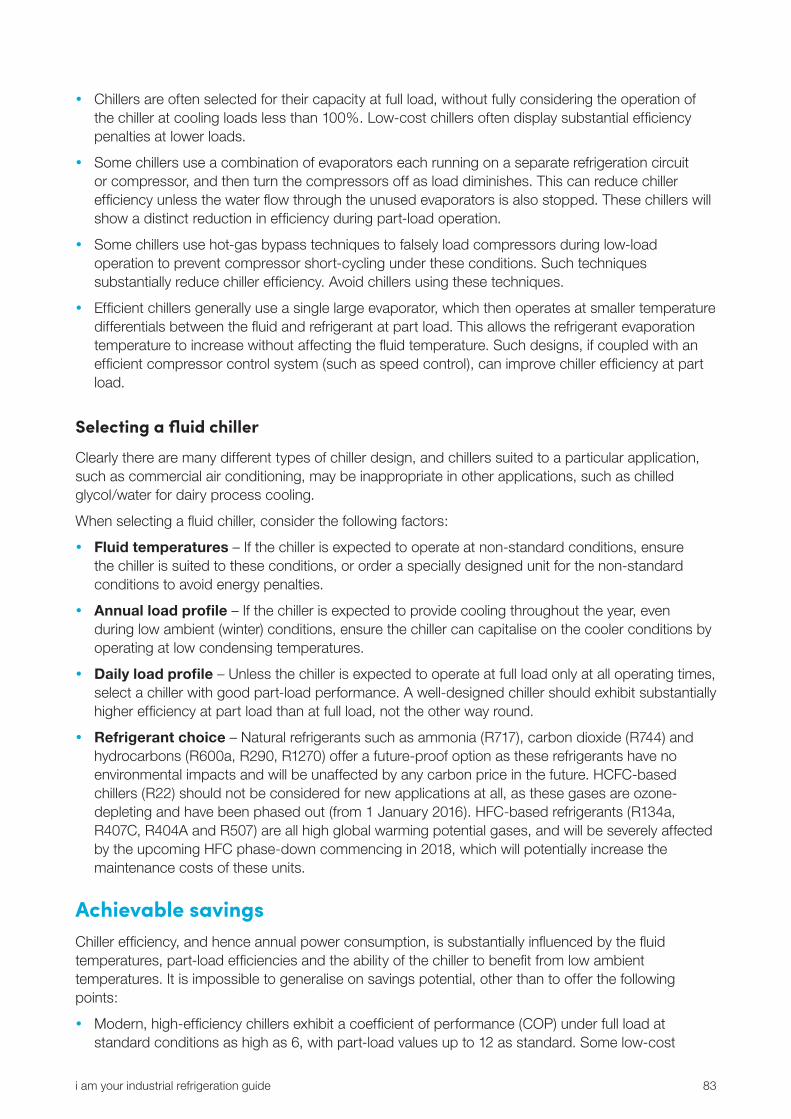
i am your industrial refrigeration guide 83
y Chillers are often selected for their capacity at full load, without fully considering the operation of the chiller at cooling loads less than 100%. Low-cost chillers often display substantial efficiency penalties at lower loads.
y Some chillers use a combination of evaporators each running on a separate refrigeration circuit or compressor, and then turn the compressors off as load diminishes. This can reduce chiller efficiency unless the water flow through the unused evaporators is also stopped. These chillers will show a distinct reduction in efficiency during part-load operation.
y Some chillers use hot-gas bypass techniques to falsely load compressors during low-load operation to prevent compressor short-cycling under these conditions. Such techniques substantially reduce chiller efficiency. Avoid chillers using these techniques.
y Efficient chillers generally use a single large evaporator, which then operates at smaller temperature differentials between the fluid and refrigerant at part load. This allows the refrigerant evaporation temperature to increase without affecting the fluid temperature. Such designs, if coupled with an efficient compressor control system (such as speed control), can improve chiller efficiency at part load.
Selecting a fluid chiller
Clearly there are many different types of chiller design, and chillers suited to a particular application, such as commercial air conditioning, may be inappropriate in other applications, such as chilled glycol/water for dairy process cooling.
When selecting a fluid chiller, consider the following factors:
y Fluid temperatures – If the chiller is expected to operate at non-standard conditions, ensure the chiller is suited to these conditions, or order a specially designed unit for the non-standard conditions to avoid energy penalties.
y Annual load profile – If the chiller is expected to provide cooling throughout the year, even during low ambient (winter) conditions, ensure the chiller can capitalise on the cooler conditions by operating at low condensing temperatures.
y Daily load profile – Unless the chiller is expected to operate at full load only at all operating times, select a chiller with good part-load performance. A well-designed chiller should exhibit substantially higher efficiency at part load than at full load, not the other way round.
y Refrigerant choice – Natural refrigerants such as ammonia (R717), carbon dioxide (R744) and hydrocarbons (R600a, R290, R1270) offer a future-proof option as these refrigerants have no environmental impacts and will be unaffected by any carbon price in the future. HCFC-based chillers (R22) should not be considered for new applications at all, as these gases are ozone-depleting and have been phased out (from 1 January 2016). HFC-based refrigerants (R134a, R407C, R404A and R507) are all high global warming potential gases, and will be severely affected by the upcoming HFC phase-down commencing in 2018, which will potentially increase the maintenance costs of these units.
Achievable savings Chiller efficiency, and hence annual power consumption, is substantially influenced by the fluid temperatures, part-load efficiencies and the ability of the chiller to benefit from low ambient temperatures. It is impossible to generalise on savings potential, other than to offer the following points:
y Modern, high-efficiency chillers exhibit a coefficient of performance (COP) under full load at standard conditions as high as 6, with part-load values up to 12 as standard. Some low-cost

84 Office of Environment and Heritage
chillers do not exceed COP values of 4 at full load, and these values reduce to below 2 at part-load in some cases. An inefficient chiller can incur power penalties between 25% and 40%, depending on usage, when compared to an efficient counterpart. This extreme variance in the market is often not well understood, or even believed.
y A chiller designed to fully utilise low ambient temperatures can exhibit power consumption reductions of as high as:
y 30% at typical Sydney winter conditions (10°C), compared to chillers that may limit condensing temperature to above 22°C, which represents a typical lower limit for centrifugal chillers
y 50% compared to chillers that may limit condensing temperature to above 25°C, which represents a typical limit for DX screw chillers using R134a.
y An ammonia-based process chiller operating at a supply temperature of –5°C will typically consume 30% to 50% less power than an equivalent R407C, R404A or R507 chiller operating at summer conditions, and 50% to 60% less at winter conditions (10°C).
Very significant energy savings can be achieved with appropriate chiller selection, and the additional capital cost of dedicated process chillers can be amortised in a short time in many process cooling applications. See Appendix B for more details.
Case study: Riverina FreshRiverina Fresh, Wagga Wagga, has implemented a chiller replacement project that has resulted in 760 megawatt hours of electricity savings a year with a payback period of less than three years.
Table 24: Riverina Fresh energy savings and payback
Electricity savings (MWh p.a.)
Energy cost savings ($p.a.)
Other cost savings (e.g. maintenance) ($p.a.)
Total cost savings ($p.a.)
Capital cost ($)
Payback period (years)
GHG savings (tonnes CO2 p.a.)
ESCs (number of certificates)
760 159,000 0 159,000 460,000 2.9 730 806
Riverina Fresh Pty Ltd operates a milk processing facility at Wagga Wagga, the only one in the Riverina area, with its Riverina Fresh brand providing white and flavoured milk, yogurt and dairy desserts.
The refrigeration plant was consisting of an ammonia chiller, an R22 chiller and also multiple individual freon circuits. It was responsible for most of the site’s energy consumption. Also, the site was scheduled for increased production, but the existing refrigeration plant did not have capacity to support the increase. A chiller upgrade was inevitable, so it provided a compelling opportunity for efficiency improvement as well as capacity increase.
The existing R22 chiller was required to act as an ‘ice bank’ – a practice in which the chiller produces ice during periods of low load, so that it can use this stored energy during peak load. This is a particularly inefficient practice – it is preferable to operate a chiller with capacity for peak load.
Replacing the R22 chiller also presented an opportunity for a much better environmental outcome. R22 is a type of HCFC which is a substance with significant ozone-depleting

i am your industrial refrigeration guide 85
characteristics. It also has an extremely high global warming potential of 1780, indicating that the global warming effect of R22 is 1780 times larger than that of carbon dioxide. These two properties of R22 refrigerant are the reason for its phase-out.
Riverina Fresh selected a new chiller run on ammonia. Although the unit is larger than the original unit, it is more efficient and has a far smaller environmental footprint. The replacement has resulted in an annual electricity saving of 760 megawatt hours.
Figure 33: Water-cooled ammonia chiller at Riverina Fresh, Wagga Wagga
Figure 34: Riverina Fresh’s chiller system overview

86 Office of Environment and Heritage
Technology 13: Improved chiller fluid circuit design and control
5-20% PLANT ENERGY SAVINGS OF UP TO
Overview y Principle: fluid chiller efficiency is improved by decommissioning fluid bypass lines and
maximising fluid return temperature.
y Benefits: optimises chiller performance.
y Savings: typical plant energy savings can be 5 to 20%.
y Ease of implementation: involves installing pump VSDs and control valves.
Photo: Wat Als Photography/OEH

i am your industrial refrigeration guide 87
PrinciplesThe performance of systems using chilled water or chilled glycol and water depends on the suitability of the chiller and on the design and operation of the circuit (often referred to as the ‘field’). Where the field design is ineffective, part-load and even full-load operation of the chiller can be compromised, resulting in reduced available capacity and increased power consumption.
Fundamentally the field design and control needs to match the chiller to the load in the most effective and efficient manner. If fluid flows in the system are not modulated or balanced, mixing of cold and warm fluid streams can occur. Thus, the fluid return temperature to the chiller is reduced unnecessarily, compromising both the effective cooling performance and the energy efficiency of the chiller.
Chillers are designed such that, in normal operating conditions, the temperature differential across the chiller (the temperature difference between fluid return and supply temperature) is generally in the range of 4°C to 6°C with the fluid flow rate at the design value. The refrigeration capacity of the chiller is then given by the following relationship:
Q = m’ x CP x rT
where:
Q = chiller refrigeration capacity (kW)
m’ = mass flow rate of chilled fluid (kg/sec)
CP = specific heat capacity of chilled fluid (kJ/kg K)
rT = temperature differential between fluid entering and leaving the chiller (°C or K).
FactboxThe temperature differential is essential to maintain chiller efficiency. If the chiller operates at lower differential temperatures, by increasing the fluid flow rate for example, the mean fluid temperature in the chiller is reduced. This in turn causes the chiller to operate at lower evaporation temperature to maintain refrigeration capacity, thereby reducing chiller efficiency and raising power consumption.
Figure 35: Example of three-way valve control mixing warm and cold fluid streams

88 Office of Environment and Heritage
Plant benefits Plant benefits include maximised efficiency of the chilled water system at all load conditions.
Achievable savings Often, the field is designed such that a chiller is subject to constant fluid flow rates and must use bypass flow control at the cooling stations to maintain chiller flow. For reasons explained above, this is inefficient. Substantial energy savings are achievable by converting the system to variable flow and two-way flow control at the cooling stations. The savings achievable depend on:
y the part-load efficiency of the chiller. Higher savings are achieved if the chiller exhibits higher efficiency at part load than at full load
y the extent of bypass flow control and constant flow used at the cooling stations in the system
y annual and daily load profiles.
Typically, chiller power savings in the range of 5% to 20% are achievable by maximising fluid return temperatures.
ImplementationAt all times, the overriding principle of field design and control is to maximise the fluid return temperature to the chiller under all operating conditions. This has several significant implications for system design:
y The flow rate through the chiller must be reduced in proportion to the actual cooling load. If the load drops by 50%, the flow rate is also reduced by 50%, to maintain the return temperature to the chiller. This maintains or increases efficiency, given that good chillers have higher part-load efficiency. If the flow rate is not adjusted appropriately, lower return temperatures negate the benefits of increased chiller part-load efficiency.
y The flow of chilled fluid to devices that use cold fluid should be controlled, by turning the flow on or off when these devices are in use or off, respectively, or by modulating the flow to the device in proportion to the instantaneous cooling load of the device.
y All forms of bypass flow in the system should be eliminated. Bypass flow control allows ‘unused’ cold fluid to return to the chiller or buffer tank via the return line, effectively causing the cold fluid to mix with the heated fluid in the return line, resulting in a reduction of return temperature and therefore chiller performance as mentioned above (see figure 35).
Ideally, as the field load reduces, so should the fluid flow rate. This maintains the temperature differential across the chiller, maintaining chiller efficiency. This can be achieved with a single circuit arrangement (figure 34) or with a primary/secondary arrangement (figure 35) with the following key modifications:
y Prioritise use of two-way modulating or on–off control and avoiding use of three-way bypass control or constant flow arrangements. This achieves variable system flow in proportion to the load.
y Use a variable-speed pump to deliver a variable flow proportional to the load
y Use an end-of-line pressure sustaining valve to maintain pressure when the pump reaches minimum speed (generally 20 hertz). This causes some unavoidable mixing of supply and return flow.
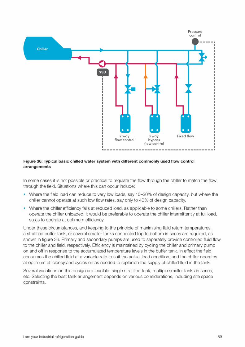
i am your industrial refrigeration guide 89
2 wayflow control
3 way bypass
flow control
Fixed flow
Pressurecontrol
VSD
Chiller
Figure 36: Typical basic chilled water system with different commonly used flow control arrangements
In some cases it is not possible or practical to regulate the flow through the chiller to match the flow through the field. Situations where this can occur include:
y Where the field load can reduce to very low loads, say 10–20% of design capacity, but where the chiller cannot operate at such low flow rates, say only to 40% of design capacity.
y Where the chiller efficiency falls at reduced load, as applicable to some chillers. Rather than operate the chiller unloaded, it would be preferable to operate the chiller intermittently at full load, so as to operate at optimum efficiency.
Under these circumstances, and keeping to the principle of maximising fluid return temperatures, a stratified buffer tank, or several smaller tanks connected top to bottom in series are required, as shown in figure 36. Primary and secondary pumps are used to separately provide controlled fluid flow to the chiller and field, respectively. Efficiency is maintained by cycling the chiller and primary pump on and off in response to the accumulated temperature levels in the buffer tank. In effect the field consumes the chilled fluid at a variable rate to suit the actual load condition, and the chiller operates at optimum efficiency and cycles on as needed to replenish the supply of chilled fluid in the tank.
Several variations on this design are feasible: single stratified tank, multiple smaller tanks in series, etc. Selecting the best tank arrangement depends on various considerations, including site space constraints.
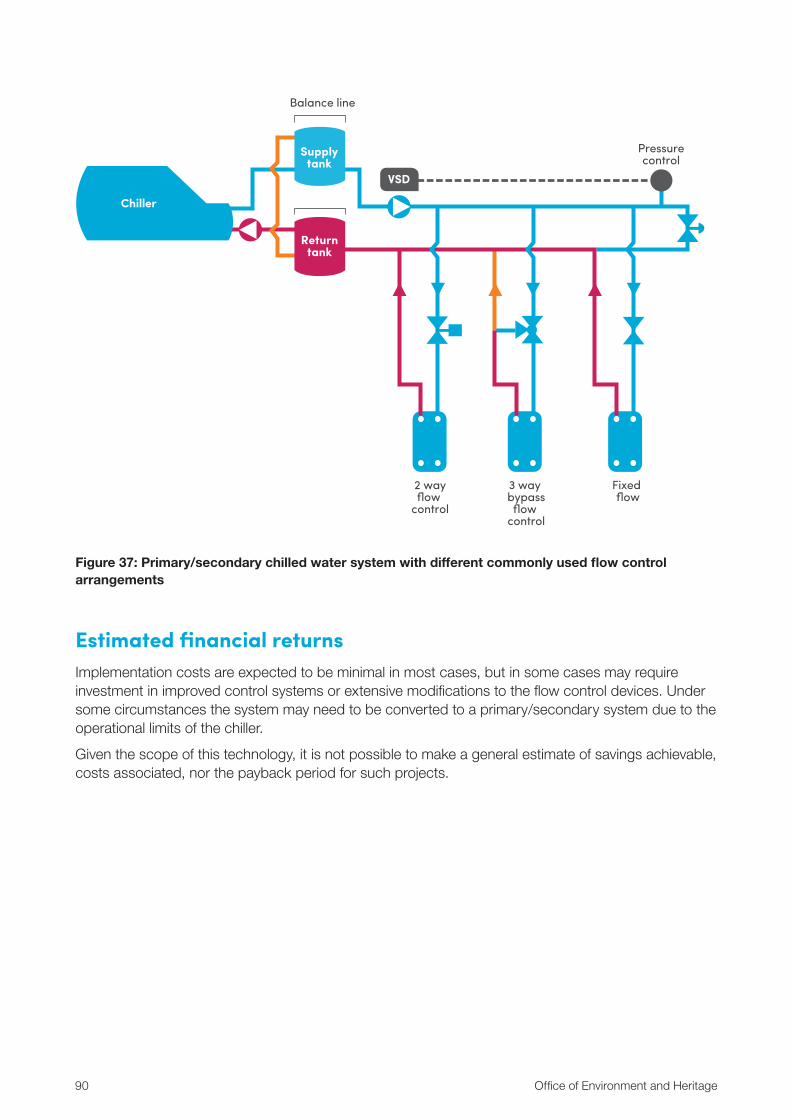
90 Office of Environment and Heritage
2 wayflow
control
3 way bypassflow
control
Fixed flow
Balance line
Chiller
Supplytank
Returntank
VSD
Pressurecontrol
Figure 37: Primary/secondary chilled water system with different commonly used flow control arrangements
Estimated financial returnsImplementation costs are expected to be minimal in most cases, but in some cases may require investment in improved control systems or extensive modifications to the flow control devices. Under some circumstances the system may need to be converted to a primary/secondary system due to the operational limits of the chiller.
Given the scope of this technology, it is not possible to make a general estimate of savings achievable, costs associated, nor the payback period for such projects.

i am your industrial refrigeration guide 91
Case study: Radevski Cold StoresRadevski Cold Stores, Shepparton, improved its chiller fluid circuit design and this resulted in 190 megawatt hours of electricity savings a year.
Table 25: Radevski Cold Stores energy savings and payback
Electricity savings (MWh p.a.)
Energy cost savings ($p.a.)
Other cost savings (e.g. maintenance) ($p.a.)
Total cost savings ($p.a.)
Capital cost ($)
Payback period (years)
GHG savings (tonnes CO2 p.a.)
ESCs (number of certificates)
190 28,000 0 28,000 35,000 1.3 182 203
Redevski Cold Stores is a family owned business in Victoria. Its facility in Shepparton operates 16 cool rooms for fruit storage which are cooled through a chilled glycol circuit. Fruits are at ambient temperature when they are picked in February and March. After a full day of storage in the cool rooms, the fruit temperature is pulled down to around 2°C for long-term storage. Due to this type of operation, the system only operates at close to full load for about two months and at part load for the rest of the year.
Originally, chilled glycol flow rate in the system was fixed and at the end of the circuit, a ball valve was installed and widely open to bypass the ‘unused’ cold fluid, as shown in figure 38. It was estimated that around 10 to 20% of the total chilled water flow was bypassed and this number could be up to 50% when there was a low load in the cool rooms. This resulted in significant energy consumption.
To solve these issues:
y Variable speed drives VSD) have been installed on the glycol pumps to allow variable glycol flow rate in the system. The pumps can slow down to 40% of their full speed.
y The ball valve at the end of the circuit has been replaced with a motorised valve to maintain a minimum bypass flow rate. For most of the operating period, the valve is shut and the glycol flow rate is adjusted by the pump VSDs to accommodate the cool room load variation. When there is a very small load in the cool rooms, the pumps will operate at their minimum speed and the motorised valve will open slightly to bypass a small portion of the glycol flow.
These upgrades have reduced the site power consumption beyond the plant owner’s expectation.
Before this upgrade our glycol system was very unstable. The new system was developed and commissioned to combat these issues, but we also found that we can save money on energy at the same time. The new glycol system continues to work efficiently.
Peter Radevski, General Manager

92 Office of Environment and Heritage
Case study: Radevski Cold Stores
Figure 38: Before: a fully opened ball valve at the end of the circuit to bypass unused flow
Figure 39: After: a motorised valve installed at the end of the circuit

i am your industrial refrigeration guide 93
Technology 14: Variable chiller fluid temperatures
20% PLANT ENERGY SAVINGS OF UP TO
Overview y Principle: the chilled fluid temperature set-point is varied to optimise the evaporation
temperature of the chiller.
y Benefits: reduces power consumption of the chiller.
y Savings: typical plant energy savings can be up to 20%.
y Ease of implementation: involves reprogramming the chiller control system.
Photo: Wat Als Photography/OEH
94 Office of Environment and Heritage
PrinciplesIt is common industry practice to operate chilled water or glycol/water systems at fixed temperature set-points, without consideration of ambient conditions or cooling loads. In some situations, these set-point temperatures can be increased without a negative effect on the process being cooled, which has the effect of increasing the chiller efficiency and reducing power consumption.
Refrigeration systems use substantially less power if the evaporation temperature at which the system operates can be increased.
FactboxTypically, power consumption reduces by 3% for every 1°C increase in evaporation temperature and hence, fluid temperature. A 3°C increase in evaporation temperature can result in energy savings of 9%.
Some applications do not permit significant variation in fluid temperature. For example, many food processing applications, such as milk processing, use chilled water or water/glycol to cool product via a heat exchanger where steady fluid temperatures are essential in maintaining product quality and hygiene.
However, many other applications can tolerate seasonal or load-dependent variations of fluid temperature. For example, when chilled water is used for cooling processing rooms, the reduced cooling loads and lower ambient humidity levels allow chilled water temperature to be set higher during winter. In the case of fruit storage rooms cooled by glycol/water systems, the reduced cooling load during winter generally allows the fluid temperature to be increased by 2–3°C in winter compared to summer operation.
Achievable savings Where an existing chiller operates at essentially constant set-point temperatures and the temperature can be made to vary under the range of operating conditions, substantial energy savings can be achieved. These depend on the:
y nature of the application
y annual and daily load profile
y ambient conditions.
In some situations, significant variation of fluid temperatures is achievable with annual power savings as high as 20%, in others this cannot be tolerated and little potential exists.
Implementation costs are expected to be minimal in most cases (reprogramming of controls), but in some cases implementation may require investment in improved control systems.
i am your industrial refrigeration guide 95
Technology 15: Variable cooling water temperatures
15% PLANT ENERGY SAVINGS OF UP TO
Overview y Principle: variable cooling water temperature control is implemented to minimise chiller
condensing temperature when possible.
y Benefits: optimises chiller efficiency.
y Savings: typical plant energy savings can be up to 15%.
y Ease of implementation: involves programming chiller control logic and possible installation of cooling tower fan variable speed drives (VSD).
Photo: Wat Als Photography/OEH

96 Office of Environment and Heritage
Principles It is common industry practice to design and operate cooling water systems at standard conditions, such as 29.5°C inlet and 35°C return temperatures, without considering ambient conditions. This often leads to cooling water systems operating at temperatures of 25°C or above, even under winter conditions, with ambient air temperatures of 10°C or lower. This is a substantial lost opportunity for energy savings.
FactboxRefrigeration systems use substantially less power if the condensing temperature at which the system operates can be reduced. Typically, power consumption reduces by 3% for every 1°C reduction in condensing temperature. Hence a 10°C reduction in condensing temperature can result in energy savings of 30%.
FactboxIn summer conditions (in Sydney this could be 25°C wet bulb temperature), cooling water temperatures of 27°C or higher are achievable, while in winter conditions (<5°C wet bulb temperature), cooling water temperatures below 10°C could be achieved at full air-flow rate.
Water-cooled chillers require a cooling system to remove the condensing heat. Generally, this consists of a water pump, a cooling tower and piping to circulate water through the heat exchanger on the chiller and the cooling tower. The cooling water temperature depends on the ambient wet bulb temperature and the rate of air circulation through the cooling tower. However, in most systems the air flow rate is modulated by controlling the cooling tower fan speed or by bypassing the cooling tower to maintain cooling water temperature above a set minimum, typically 15°C to 20°C, sometimes higher.
Where the chiller design permits the condensing temperature to float to low values without negative impact on the chiller reliability or refrigeration capacity, considerable energy savings can be achieved by allowing the cooling water temperature to reduce to very low values, although this has to be well above 0°C to prevent any problems with ice formation during winter conditions.
In some cases, cooling water systems are shared within a facility, and cooling water is provided to a range of devices requiring cooling. In some cases these other devices require constant cooling water temperatures and hence the design of the cooling water system on site may need to be reviewed to ensure these other devices are not affected by excessively low cooling water temperatures.
Achievable savings Where an existing water-cooled chiller operates at essentially standard cooling water conditions, greater than 25°C, the cooling water temperature can ‘float’ to suit ambient conditions, so substantial energy savings are achievable. These savings also depend on:
y the annual and daily load profile
y the suitability of the chiller for floating condensing temperature operation.
Typically, annual savings of 5% to 15% can be achieved for process cooling applications if cooling water temperatures are fully floated. Implementation costs could be minimal in some cases, such as the reprogramming of controls, but in other cases may require the installation of cooling tower fan variable speed drives (VSD).

i am your industrial refrigeration guide 97
Case study: Elf MushroomsElf Mushrooms implemented variable cooling water temperature control for its water-cooled chiller system, and reduced its energy costs by 8%, saving an estimated $30,000 a year.
Table 26: Elf Mushrooms energy savings and payback
Electricity savings (MWh p.a.)
Energy cost savings ($p.a.)
Other cost savings (e.g. maintenance) ($p.a.)
Total cost savings ($p.a.)
Capital cost ($)
Payback period (years)
GHG savings (tonnes CO2 p.a.)
ESCs (number of certificates)
200 30,000 0 30,000 13,000 0.4 192 212
Based in Sydney, Elf Mushrooms is a 100% Australian, family-owned business. Founded in 1960, Elf has 110 full-time equivalent staff, with year-round 24/7 operations delivering 3 million kilograms of mushrooms throughout the country.
Mushrooms need a climate-controlled environment throughout their growing cycle. This requires constant refrigeration to control humidity and temperature in 21 growing rooms – with cooling capacity provided by a large chiller and twin cooling towers. Elf’s energy bill is more than $360,000 each year.
The issue for Elf Mushrooms was that the cooling water temperature in its chiller was simply set to minimum. In other words, the cooling tower fans were programmed to maintain a constant cooling water supply temperature of 22°C, regardless of ambient conditions. This meant that in summer, the fans were operating at maximum speed every day – trying to reach 22°C even when this was not achievable.
To fix this, control logic has been installed to optimise total power consumption. A new controller and sensors have been added, so the controller can monitor the ambient wet bulb temperature, the cooling water temperature and the percentage load from the chiller – and then calculate the best combination of chiller and condenser fan energy consumption at any given time.
Because the cooling tower fans were already fitted with variable speed drives, the upgrade was achieved without major changes to our existing equipment. This meant our refrigeration plant only needed to be shut down for a few brief periods.
David Tolsen, Elf Mushrooms Managing Director

98 Office of Environment and Heritage
Case study: Elf Mushrooms
Figure 40: Two cooling towers at Elf Mushrooms
Figure 41: Cooling tower VSD and cooling water temperature controller at Elf Mushrooms
VSDController
VSD
Controller

i am your industrial refrigeration guide 99
Appendix A: Measurement and verification plansThis appendix contains a measurement and verification (M&V) plan for each of the 15 technologies discussed in this guide. Office of Environment and Heritage recommends you work with an Accredited Certified Measurement and Verification Professional (CMVP) to further develop a more detailed M&V plan for each specific project you will undertake.
Table A1: Measurement and verification plans for the 15 technologies
Technology Measurement and verification plan
Technology 1: Variable head pressure control and variable inter-stage pressure control
Implementing this technology is expected to affect the power consumption of both compressors and condensers. The following parameters will be logged during baseline and post-implementation periods:
y power consumption of relevant compressors
y power consumption of condensers
y ambient wet bulb temperature
y any production data that can best describe the load variation of the refrigeration system.
Technology 2: Automated compressor staging and capacity control
Implementing this technology is expected to affect the power consumption of relevant compressors. The following parameters will be logged during baseline and post-implementation periods:
y power consumption of relevant compressors
y ambient wet bulb temperature
y any production data that can best describe the load variation of the refrigeration system.
Technology 3: Water and air purging from ammonia systems
Implementing this technology is expected to affect the power consumption of the whole refrigeration system. The following parameters will be logged during baseline and post-implementation periods:
y incoming power of the refrigeration plant room
y ambient wet bulb temperature
y any production data that can best describe the load variation of the refrigeration system.
Technology 4: Heat recovery from discharge gas and oil cooling
The M&V approach will be different from site to site, depending on the arrangement of the hot water system.
Technology 5: Variable defrost timing and termination
Implementing this technology is expected to affect the power consumption of the whole refrigeration system. The following parameters will be logged during baseline and post-implementation periods:
y incoming power of the refrigeration plant room
y ambient wet bulb temperature
y any production data that can best describe the load variation of the refrigeration system.

100 Office of Environment and Heritage
Technology Measurement and verification plan
Technology 6: Variable cold store temperatures
Implementing this technology is expected to affect the power consumption of the whole refrigeration system. The following parameters will be logged during baseline and post-implementation periods:
y incoming power of the refrigeration plant room
y ambient wet bulb temperature
y any production data that can best describe the load variation of the refrigeration system.
Technology 7: Variable evaporator fan speeds
Implementing this technology is expected to affect the power consumption of the whole refrigeration system. The following parameters will be logged during baseline and post-implementation periods:
y power consumption of all relevant evaporators
y incoming power of the refrigeration plant room
y ambient wet and dry bulb temperatures
y any production data that can best describe the load variation of the refrigeration system.
Technology 8: Condensate sub-cooling techniques
Implementing this technology is expected to affect the power consumption of the high-stage compressors. The following parameters will be logged during baseline and post-implementation periods:
y power consumption of all high-stage compressors
y ambient wet bulb temperatures
y any production data that can best describe the load variation of the refrigeration system.
Technology 9: Ammonia plant process design review
Implementing this technology is expected to affect the power consumption of the whole refrigeration system. The following parameters will be logged during baseline and post-implementation periods:
y incoming power of the refrigeration plant room
y ambient wet and dry bulb temperatures
y any production data that can best describe the load variation of the refrigeration system.
Technology 10: Improved industrial screw compressor oil feed control and oil cooling
Implementing this technology is expected to affect the power consumption of the relevant compressors. The following parameters will be logged during baseline and post-implementation periods:
y power consumption of all relevant compressors
y ambient wet bulb temperatures
y any production data that can best describe the load variation of the refrigeration system.

i am your industrial refrigeration guide 101
Technology Measurement and verification plan
Technology 11: Screw compressor degradation check
Implementing this technology is expected to affect the power consumption of relevant compressors and the entire system. The following parameters will be logged during baseline and post-implementation periods:
y power consumption of the relevant compressors
y power consumption of the entire refrigeration system
y ambient wet bulb temperatures
y any production data that can best describe the load variation of the refrigeration system.
Technology 12: Fluid chiller selection for energy efficiency
Implementing this technology is expected to affect the power consumption of the entire refrigeration system. The following parameters will be logged during baseline and post-implementation periods:
y power consumption of the entire refrigeration system
y ambient wet and dry bulb temperatures
y any production data that can best describe the load variation of the refrigeration system.
Technology 13: Improved chiller fluid circuit design and control
Implementing this technology is expected to affect the power consumption of both chillers and pumps. The following parameters will be logged during baseline and post-implementation periods:
y power consumption of the chillers
y power consumption of the chilled fluid supply pumps
y ambient wet and dry bulb temperatures
y any production data that can best describe the load variation of the refrigeration system.
Technology 14: Variable chiller fluid temperatures
Implementing this technology is expected to affect the power consumption of the chillers. The following parameters will be logged during baseline and post-implementation periods:
y power consumption of the chillers
y ambient wet and dry bulb temperatures
y any production data that can best describe the load variation of the refrigeration system.
Technology 15: Variable cooling water temperatures
Implementing this technology is expected to affect the power consumption of both chillers and cooling towers. The following parameters will be logged during baseline and post-implementation periods:
y power consumption of chillers
y power consumption of cooling towers
y ambient wet bulb temperature
y any production data that can best describe the load variation of the refrigeration system.

102 Office of Environment and Heritage
Appendix B: Modelling detailsTechnology 1: Variable head pressure control and variable inter-stage pressure control
Variable head pressure control
Modelling suggests that, compared to a system with fixed head pressure settings, variable head pressure control (VHPC) can generate average annual energy savings of:
y for fixed head pressure 25°C – 9% to 12% of high-stage compressor power consumption
y for fixed head pressure 30°C – 20% to 25% of high-stage compressor power consumption
y for fixed head pressure 35°C – 30% to 35% of high-stage compressor power consumption.
Notes:
1 These figures are based on modelling of three typical applications as explained below.
2 These indicated savings are only achievable if the control logic is suitably optimised.
Figure B1 illustrates the annual energy saving profiles for a cold store running at 25°C, 30°C and 35°C fixed head pressure for 24 hours a day, seven days a week. Profiles for production facilities operating 16 hours a day, five days a week and 16 hours a day, seven days a week are similar in trend and magnitude to figure B2.
0
5
10
15
20
25
30
35
40
Jan Feb Mar Apr May Jun Jul Aug Sep Oct Nov Dec
Savi
ngs
%
T_c = 25 T_c = 30 T_c = 35
Figure B1: Annual energy saving profile due to variable head pressure control for a typical cold store application

i am your industrial refrigeration guide 103
Figure B2 illustrates the energy savings possible with VHPC for various applications when compared to a system with fixed condensing temperatures of 25°C, 30°C or 35°C.
0
5
10
15
20
25
30
35
Production 16/7Production 16/5Cold storage
353025
Condensing temperature setpoint for fixed head pressure operation (°C)
Ener
gy s
avin
gs (%
)
Figure B2: Average annual energy savings due to variable head pressure control for various typical applications
Annual energy savings for the following three typical operating regimes have been modelled.
y A cold store with a variable load profile where plant load oscillates between 60% and 100% of maximum plant capacity based on the time of the day.
y A 16/7 production schedule which operates at 100% of maximum plant capacity for two shifts every day and at 30% at other times. This is representative of having both production and storage on such sites.
y A 16/5 production schedule that operates at 100% plant capacity for two shifts every week day and at 30% at other times. This is representative of both production and storage on such sites.
The following assumptions have been made for each operating regime:
y refrigerant used – ammonia
y ambient conditions – annual weather conditions for Sydney
y condenser/ambient wet bulb approach (temperature difference)
y linear with 10°C approach at 90% plant load and 3°C approach at 10% plant load
y minimum condensing temperature equals 20°C, factoring in practical considerations.
The following methodology was used to calculate annual savings for each regime over one year.
1. The condensing temperature was calculated for every hour of the year using a derived load profile and ambient wet bulb temperature data.
2. The efficiency of the system with variable head pressure control was then calculated based on the condensing temperature and a fixed suction temperature of the system.

104 Office of Environment and Heritage
3. The coefficient of performance of the conventional system with a fixed head pressure setting was then calculated. Each of the regimes was run three times, using condensing temperatures fixed at 25°C, 30°C and 35°C.
4. For the 25°C scenario, the system attempts to maintain 25°C condensing temperature as far as the load and ambient conditions permit. As the load and ambient wet bulb temperature increase, the condensing temperature increases correspondingly. Below 25°C, savings are minimal as both systems run at similar head pressures. The savings due to variable head pressure control are possible between condensing temperatures of 20°C and 25°C, which is mainly during the cold winter months.
5. The same argument is true for scenarios of 30°C and 35°C. Savings increase as the fixed head pressure setting increases, because the variable head pressure control can run below the fixed head pressure control set-point for a greater portion of the year.
Achievable savings depend on the following:
y The application: variable production cycles, such as batch cycles and cold storage applications have variable loads and greater savings potential compared to plants with fixed loads i.e. facilities having a constant throughput profile.
y Heat rejection equipment in the plant: if condensers are oversized, energy savings are achieved by running lower head pressure and lower fan speed where possible.
y Oil separator design: when a plant runs at lower head pressures than design, the discharge gas velocities increase and so the velocity through the oil separator increases. At a certain point, the gas velocity could be so high that the oil is carried over with the discharge gas and accumulates in the low-pressure vessel of the plant. This will result in excessive oil consumption and increased maintenance requirements. A plant with oversized oil separators can handle greater gas velocities, permitting lower head pressures and greater energy savings compared to plants with smaller oil separators.
Variable inter-stage pressure control
For a plant with a suction temperature of –30°C and a condensing temperature of 35°C, figure B3 illustrates the relationship between achievable savings and the inter-stage temperature/pressure.
-1.0
-0.5
0.0
0.5
1.0
1.5
2.0
20-2-4-6-8-10
Ener
gy s
avin
gs (%
)
Inter stage saturation temperature (°C)
Figure B3: Savings associated with varying inter-stage pressure on a two-stage plant

i am your industrial refrigeration guide 105
Figure B3 illustrates the effect of varying inter-stage pressure on the efficiency of a refrigeration plant. Results are compared against a plant with an inter-stage temperature of –10°C. The optimum inter-stage pressure of this system corresponds to a saturation temperature of –4°C. At an inter-stage temperature above –4°C, the increase in absorbed power of the low-stage system is greater than the decrease in absorbed power of the high-stage system. Conversely, at an inter-stage temperature below –4°C, the increase in absorbed power of the high-stage system is greater than the decrease in absorbed power of the low-stage system.
Technology 2: Automated compressor staging and capacity controlTo calculate the savings achievable, a single-stage refrigeration plant with two compressors using this technology was modelled against the same plant using conventional compressor staging control. Table B1 presents:
y the energy savings achievable at instantaneous plant loads
y the total annual energy savings achievable, by aggregating instantaneous energy savings over the annual plant load profile presented in figure 1: Refrigeration plant annual usage profile used for energy savings calculations.
Table B1: Energy savings according to plant load
Plant load Energy saving
10% 40%
20% 33%
30% 24%
40% 41%
50% 32%
60% 14%
70% 6%
80% 5%
90% 3%
100% 0%
Total annual energy savings
24%
Over a typical year, the following methodology was used to calculate annual savings:
y the lead compressor is variable speed controlled
y the lag compressor is slide valve controlled between 75% and 100%
y the comparison is done against a plant where the compressors have no variable speed drives (VSD) or proper slide valve control – this is based on observations in real time on a certain plant
y the observations indicated the lag compressor would turn on when the lead compressor was at 75% load or higher; the calculations have been conducted on this basis
y the usage profile presented in figure 1 was used for the purpose of this analysis.

106 Office of Environment and Heritage
Technology 9: Ammonia plant process design review
1: Removing bottlenecks
The energy savings indicated in figure 28 assume a 500 kilowatts refrigeration load and a possible elevation in suction temperature by 5°C due to bottleneck removal, aggregated over the load profile presented in figure 1.
Table B2: Energy savings due to bottleneck removal
Energy consumption of conventional system (kWh/year)
Energy consumption of improved system (kWh/year)
Energy savings (kWh/year)
Energy cost savings ($/year)
677,000 577,000 100,000 15,000
1 Average cost of power is assumed to be $0.15 per kilowatt hour.
2 The usage profile presented in figure 1 has been used for this analysis.
2: Suction splitting
For a refrigeration system with a peak freezer load of 500 kilowatt aggregated over the load profile presented in figure 1, the estimated cost savings and payback are:
Table B3: Energy savings due to suction splitting
Energy consumption of conventional system (kWh/year)
Energy consumption of improved system (kWh/year)
Energy savings (kWh/year)
Energy cost savings ($/year)
545,000 471,000 74,000 11,100
1 Average cost of power is assumed to be $0.15 per kilowatt hour.
2 The usage profile presented in Figure 1 has been used for this analysis.
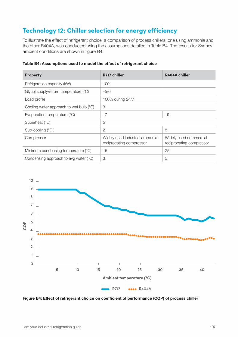
i am your industrial refrigeration guide 107
Technology 12: Chiller selection for energy efficiencyTo illustrate the effect of refrigerant choice, a comparison of process chillers, one using ammonia and the other R404A, was conducted using the assumptions detailed in Table B4. The results for Sydney ambient conditions are shown in figure B4.
Table B4: Assumptions used to model the effect of refrigerant choice
Property R717 chiller R404A chiller
Refrigeration capacity (kW) 100
Glycol supply/return temperature (°C) –5/0
Load profile 100% during 24/7
Cooling water approach to wet bulb (°C) 3
Evaporation temperature (°C) –7 –9
Superheat (°C) 5
Sub-cooling (°C ) 2 5
Compressor Widely used industrial ammonia reciprocating compressor
Widely used commercial reciprocating compressor
Minimum condensing temperature (°C) 15 25
Condensing approach to avg water (°C) 3 5
0
1
2
3
4
5
6
7
8
9
10
CO
P
Ambient temperature (°C)
5 10 15 20 25 30 35 40
R404AR717
Figure B4: Effect of refrigerant choice on coefficient of performance (COP) of process chiller

108 Office of Environment and Heritage
Appendix C: Glossary ACP Accredited Certificate Provider (Energy Savings Certificates)
bottleneck a plant design feature that forces the rest of the plant to run inefficiently
CMS control management system
COP coefficient of performance = ratio of cooling duty to consumed power
DX direct expansion
EEV electronic expansion valve
ESC Energy Savings Certificate
ESS NSW Government Energy Savings Scheme
field heat exchangers outside of plant room doing useful cooling work, and connected to plant via piping system
HCFC hydrochlorofluorocarbon (a synthetic, ozone-depleting and high global warming refrigerant)
HFC hydrofluorocarbon (a synthetic, high global warming refrigerant)
IPLV integrated part-load value
ISPC inter-stage pressure control
LPG liquid petroleum gas
M&V measurement and verification
OEH Office of Environment and Heritage
PCM phase change material
PHE plate heat exchanger
PLC programmable logic controller
purging removal of non-condensable gases or water from a refrigeration system
R134a HFC refrigerant commonly used for medium to high temperature applications
R22 hydrochlorofluorocarbon that has been phased our due to it ozone depleting and high global warming potential
R404A blended HFC refrigerant commonly used for low temperature applications
R407C blended HFC refrigerant commonly used for medium temperature applications
R507 blended HFC refrigerant commonly used for low temperature applications
R717 ammonia, a commonly used natural refrigerant
R744 carbon dioxide, a natural refrigerant increasingly being used for low and medium temperature applications
SCT saturated condensing temperature
SST saturated suction temperature

i am your industrial refrigeration guide 109
static single point/one time; as in:
static implementation: control system with logic adjustable only by local program changes
static optimisation: control system with logic optimised for one operating condition only
VHPC variable head pressure control
VIPC variable inter-stage pressure control
VSD variable speed drive
WB Wet bulb