Hypothesis Testing and Interval Estimation

James H. Steiger

November 17, 2003

1 Topics for this Module

1. An Idealistic Special Case � When � is Known.

2. Con�dence Interval Estimation

(a) Taking a Stroll with Mr. Mu

3. Hypothesis Testing

(a) Parameter Spaces and Sample Spaces

(b) Partitioning the Parameter Space

(c) Partitioning the sample space

(d) Raw Score Rejection Rules

(e) Error Rates

i. Type I Errorii. Type II Error

(f) Statistical Power

i. Power vs. Precision

4. Test Statistics

5. Standardized Rejection Rules

6. 1-tailed vs. 2-Tailed Tests

7. In�uences on Power

1

2 An Idealistic Special Case � Statistical Pro-cedures When � is Known.

In this section, we will employ a distribution that is a standard �teachingdevice� in a number of behavioral statistics texts � statistical proceduresrelated to the distribution of the sample mean X� when the population stan-dard deviation � is known. This situation is unrealistic, in the sense that weare no more likely to know � than we are to know �. However, it turns outthat, to a surprising extent, it actually doesn�t matter much that we don�tknow �.When the population distribution is normal, the distribution of the sam-

ple mean is exactly normal, with mean �, and standard deviation �X� =

�=pN . The normality follows from the fact that the sample mean is a linear

combination of independent normal observations, and that any linear com-bination of multivariate normal normal random variables is itself normallydistributed. The mean and standard deviation of the distribution follow fromlinear combination theory.When the population distribution is not normal, the distribution of the

sample mean will often still be very close to normal in shape, because of theCentral Limit Theorem we discussed previously.We shall proceed, for a while, as if the distribution of the sample mean

can be assumed to be normal to a high degree of accuracy. We will nowexamine two key topics: interval estimation and hypothesis testing.

3 Con�dence Interval Estimation

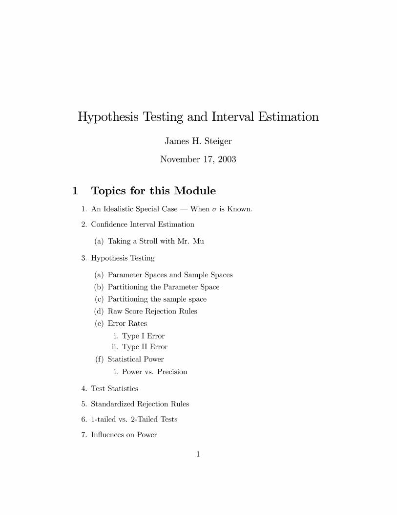
Assume, for the time being, that we know that the distribution of X� overrepeated samples is as pictured below:This graph demonstrates the distribution of X� over repeated samples.

In the above graph, as in any normal curve, 95% of the time a value willbe between Z-score equivalents of �1:96 and +1:96: These points are at araw score that is 1:96 standard deviations below the mean and 1:96 standarddeviations above the mean. Consequently, if we mark points on the graph at� � 1:96�=

pN and � + 1:96�=

pN , we will have two points between which

X� will occur 95% of the time.

2

Figure 1: The Sampling Distribution of X�

We can then say that

Pr

��� 1:96 �p

N� X� � �+ 1:96

�pN

�= :95 (1)

and, after applying some standard manipulations of inequalities, we canmanipulate the � to the inside of the equality and the X� to the outside,obtaining

Pr

�X� � 1:96

�pN� � � X� + 1:96

�pN

�= :95 (2)

Equation 2 implies that, if we take X� and add and subtract the �criticaldistance� 1:96�=

pN;we obtain an interval that contains the true �, in the

long run, 95% of the time.

3.1 Taking a Stroll with Mr. Mu

Even if you are not familiar with the manipulation of inequalities, there is away of seeing how Equation 2 follows from Equation 1. The �rst inequality

3

states that there is a critical distance, 1:96�=pN . and X� is within that

distance of � 95% of the time, over repeated samples. Now imagine that youhad a friend named Mr. Mu, and you went for a stroll with him. After acertain length of time, he turned to you and said, �You know, about 95%of the time, you�ve been walking within 2 feet of me.�You could, of course,reply that he has also been within 2 feet of you 95% of the time. The pointis, if X� is within a certain distance of � 95% of the time, it must also be thecase (because distances are symmetric) that � is within the same distance ofX� 95% of the time.

3.2 Constructing a Con�dence Interval

The con�dence interval for �, when � is known, is, for a 100(1� �)% con�-dence level, of the form

X� � z�1��=2�pN

(3)

where z�is a critical value from the standard normal curve. For example,z�:975 is equal to 1:96. At �rst this notation is somewhat di¢ cult to master.When you are talking about a 95% con�dence interval, � is equal to :05, and1� �=2 is :975:

Example 3.1 (A Simple Con�dence Interval) Suppose you are inter-ested in the average height of Vanderbilt male undergraduates, but you onlyhave the resources to sample about 64 men at random from the general popu-lation. You obtain a random sample of size 64, and �nd that the sample meanis 70:6 inches. Suppose that the population standard deviation is somehowknown to be 2:5 inches. What is the 95% con�dence interval for �?

Solution 3.1 Simply process the result of Equation 3. We have

70:6� 1:96 2:5p64

or70:6� :6125

We are 95% con�dent that the average height for the population of inter-est is between 69:99 and 71:21 inches.

4

Remark 3.1 A con�dence interval provides an indication of precision of es-timation (narrower intervals indicate greater precision), while also indicatingthe location of the parameter. Note that the width of the con�dence intervalis related inversely to the square root of N , i.e., one must quadruple N todouble the precision.

4 Hypothesis Testing

Hypothesis testing logic was imported into psychology from the �hard sci-ences,�and has dominated the landscape in behavioral statistics ever since.Hypothesis testing is most appropriate in situations where a dichotomousdecision (pass-fail, infected-clean, buy-sell) needs to be made on the basis ofdata in the face of uncertainty. Unfortunately, many situations in the socialsciences do not �t this mold. To see why, we need to investigate the logic ofhypothesis testing carefully.

4.1 Parameter Spaces and Sample Spaces

Suppose we are interested in a particular parameter, say a population mean�. The parameter space is the set of all possible values of the parameter.Often this is modeled to be the entire real number line from �1 to +1.

4.2 Partitioning the Parameter Space

Generally, we perform statistical tests to ascertain whether the parametersatis�es some restriction. The most common restriction is that it is a partic-ular value, or falls within some speci�ed range of values. This restriction iscommonly stated as a statistical hypothesis, which con�nes the parameter toa particular region of the parameter space.

De�nition 4.1 (Statistical Hypothesis) A statistical hypothesis is a state-ment delineating a region of the parameter space in which the parameter maybe found.A statistical hypothesis partitions the parameter space. Usually inour applications there will be two regions.

Hypotheses about � restrict it to a particular region of the parameterspace. Here are some examples:

� = 100

5

� < 100

60 � � � 70A very common form of statistical inference pits two hypotheses about a

statistical parameter against each other. The goal of the statistical decisionprocess is to decide between the two hypotheses. One hypothesis, labeledH0, is called the null hypothesis, and the other, labeled H1, is called thealternative hypothesis. Usually, these two hypotheses are mutually exclusiveand exhaustive, i.e., they are opposites that, taken together, exhaust allpossibilities, so that one or the other must be true.Often, in practice, the statistical null hypothesis is exactly the opposite

of what you believe, so your goal is to gather enough evidence to reject it infavor of the alternative hypothesis. Such a situation is called Reject-SupportTesting, and is by far the most common form of statistical testing in thebehavioral sciences.On occasion, the situation is reversed � the null hypothesis is what the

experimenter believes, so accepting the null hypothesis supports the exper-imenter�s theory. In such a case, the test is called Accept-Support Testing.Some of the common conventions of behavioral statistics are based on Reject-Support logic, and may be inappropriate or illogical when Accept-Supporttesting is being performed.We begin with an example of Reject-Support testing. Suppose you wished

to prove that a particular group of men has an above-average height. Theaverage height in the general population of men is known to be 70 inches.You state the statistical null hypothesis as

H0 : � � 70

and the alternative hypothesis as

H1 : � > 70

In this case, you actually believe the alternative hypothesis. Since eitherH0 or H1 (but not both) must be true, the falsity of H0 implies the truthof H1 and vice-versa. The two hypotheses partition the number line from�1 to +1 into two mutually exclusive and exhaustive regions, as shownin Figure 2. (The arrow pointing to H0 indicates that the null hypothesisregion includes the value 70.)

6

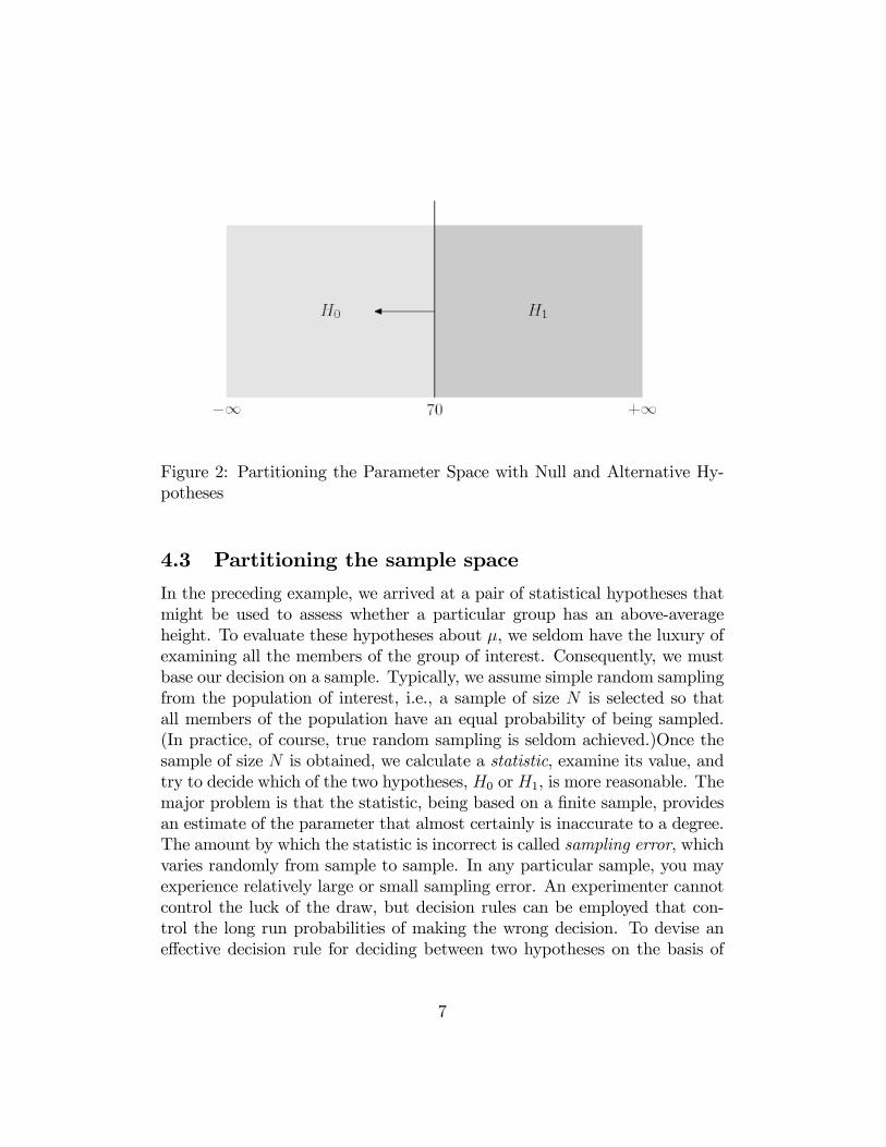
Figure 2: Partitioning the Parameter Space with Null and Alternative Hy-potheses

4.3 Partitioning the sample space

In the preceding example, we arrived at a pair of statistical hypotheses thatmight be used to assess whether a particular group has an above-averageheight. To evaluate these hypotheses about �, we seldom have the luxury ofexamining all the members of the group of interest. Consequently, we mustbase our decision on a sample. Typically, we assume simple random samplingfrom the population of interest, i.e., a sample of size N is selected so thatall members of the population have an equal probability of being sampled.(In practice, of course, true random sampling is seldom achieved.)Once thesample of size N is obtained, we calculate a statistic, examine its value, andtry to decide which of the two hypotheses, H0 or H1, is more reasonable. Themajor problem is that the statistic, being based on a �nite sample, providesan estimate of the parameter that almost certainly is inaccurate to a degree.The amount by which the statistic is incorrect is called sampling error, whichvaries randomly from sample to sample. In any particular sample, you mayexperience relatively large or small sampling error. An experimenter cannotcontrol the luck of the draw, but decision rules can be employed that con-trol the long run probabilities of making the wrong decision. To devise ane¤ective decision rule for deciding between two hypotheses on the basis of

7

a statistic, it is extremely useful to have good information about the sam-pling distribution of the statistic. Suppose a sample of size N = 25 is takenfrom a population with a normal distribution, a mean of 70, and a standarddeviation of 10. Based on our preceding discussion, we can state that, overrepeated samples, the sample mean, X�, will have a distribution that is nor-mal, with a mean of 70, and a standard deviation of 2. This fact can beexploited to create a statistical decision rule for testing the null and alter-native hypotheses discussed above. The statistical decision rule declares, inadvance, which values of the statistic X� will result in acceptance or rejectionof the null hypothesis.

4.4 A Raw Score Rejection Rule

The Sample Space of the statistic is the set of all possible values of the sta-tistic. Formally, we say that the decision rule partitions the sample spaceof the statistic. For example, suppose we are trying to decide between thehypotheses in the previous example on the basis of a sample mean X� ob-tained from a sample of 25 observations, in a case where the population isnormal and the standard deviation is known to be 10. Our construction ofa decision rule is complicated by the fact that the statistic X� has samplingerror. If X� were a perfect indicator of �, our decision rule would be thesame as the diagram in Figure 2. That is, we would decide in favor of H1 ifwe observed an X� greater than 70, otherwise we would retain H0. However,because there is sampling error, any statistical decision rule we constructwill have leave open the possibility of decision errors. Typically, this involvesconstructing a decision rule that is similar in appearance to the diagram ofthe statistical hypotheses, but is �a little fuzzy�to allow for sampling error.Suppose, for example, we decide on a one-sided or �one-tailed�decision ruleshown in Figure 2. With this rule, if a value of X� is greater than or equalto 73:29, we decide in favor of H1, otherwise we retain H0.Note that, so far, I haven�t described how I arrived at the decision rule

of Figure 3. The rule is based on a consideration of error rates.

4.5 Error Rates

Since there are two possible states of the world (H0 is either true or false)and there are only two possible decisions, there are only 4 possible outcomes,shown in Table 1.

8

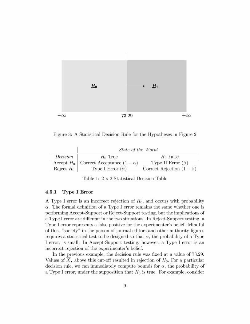
Figure 3: A Statistical Decision Rule for the Hypotheses in Figure 2

State of the World

Decision H0 True H0 FalseAccept H0 Correct Acceptance (1� �) Type II Error (�)Reject H0 Type I Error (�) Correct Rejection (1� �)

Table 1: 2� 2 Statistical Decision Table

4.5.1 Type I Error

A Type I error is an incorrect rejection of H0, and occurs with probability�. The formal de�nition of a Type I error remains the same whether one isperforming Accept-Support or Reject-Support testing, but the implications ofa Type I error are di¤erent in the two situations. In Reject-Support testing, aType I error represents a false positive for the experimenter�s belief. Mindfulof this, �society�in the person of journal editors and other authority �guresrequires a statistical test to be designed so that �, the probability of a TypeI error, is small. In Accept-Support testing, however, a Type I error is anincorrect rejection of the experimenter�s belief.In the previous example, the decision rule was �xed at a value of 73:29.

Values of X� above this cut-o¤ resulted in rejection of H0: For a particulardecision rule, we can immediately compute bounds for �, the probability ofa Type I error, under the supposition that H0 is true. For example, consider

9

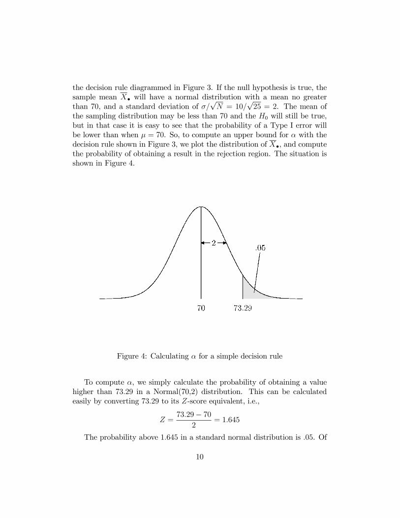
the decision rule diagrammed in Figure 3. If the null hypothesis is true, thesample mean X� will have a normal distribution with a mean no greaterthan 70, and a standard deviation of �=

pN = 10=

p25 = 2. The mean of

the sampling distribution may be less than 70 and the H0 will still be true,but in that case it is easy to see that the probability of a Type I error willbe lower than when � = 70. So, to compute an upper bound for � with thedecision rule shown in Figure 3, we plot the distribution of X�, and computethe probability of obtaining a result in the rejection region. The situation isshown in Figure 4.

Figure 4: Calculating � for a simple decision rule

To compute �, we simply calculate the probability of obtaining a valuehigher than 73:29 in a Normal(70,2) distribution. This can be calculatedeasily by converting 73:29 to its Z-score equivalent, i.e.,

Z =73:29� 70

2= 1:645

The probability above 1:645 in a standard normal distribution is :05. Of

10

course, the value 73:29, which yields the familiar :05 value for �, did not arriveout of thin air. Rather, it was calculated, deliberately, to yield the value :05.Speci�cally, we know that, for the one-sided test to yield an � value of :05,the area under the normal curve to the left of the decision point must be:95, and the area to its right must be :05. Scanning down the normal curvetable, we �nd that the Z-score value for the decision criterion must be 1:645.Next, we must convert this value to a point in the sampling distribution ofthe sample mean, which, under the null hypothesis, has a mean of 70 and astandard deviation of 2. Since we must have

X� � 702

= 1:645

it trivially follows that, in this case, the critical value of X�separating theH0 and H1 decision regions must be

X� = (2)(1:645) + 70 = 73:29

Note that this calculation is tedious, and that the raw score rejectionpoint will generally change with each new situation. Fortunately, there is away around this tedium.

4.5.2 Type II Error

A Type II error is an incorrect acceptance of H0;and occurs with probability�. In Reject-Support testing, a Type II error represents an incorrect failure tosupport the experimenter�s belief, i.e., a false negative for the experimenter�sbelief. A Type II error represents (in Reject-Support testing) a potentialdebacle for the experimenter � the experimenter�s belief is correct, but thestatistical test fails to detect this! It is therefore important for the Reject-Support tester to take steps to assure that � is small. Once a decision ruleis set, � may be calculated by presupposing an e¤ect size, i.e., an amount bywhich the null hypothesis is false.

4.6 Statistical Power

Statistical Power is de�ned as 1��. The amount by which the null hypothesisis false is called an experimental e¤ect. One can think of an experimentale¤ect as a signal, and statistical power as the ability to detect the signal. For

11

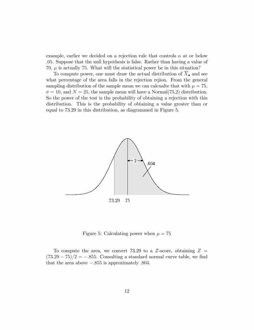
example, earlier we decided on a rejection rule that controls � at or below:05. Suppose that the null hypothesis is false. Rather than having a value of70, � is actually 75. What will the statistical power be in this situation?To compute power, one must draw the actual distribution of X� and see

what percentage of the area falls in the rejection rejion. From the generalsampling distribution of the sample mean we can calcualte that with � = 75,� = 10, and N = 25, the sample mean will have a Normal(75,2) distribution.So the power of the test is the probability of obtaining a rejection with thisdistribution. This is the probability of obtaining a value greater than orequal to 73.29 in this distribution, as diagrammed in Figure 5.

Figure 5: Calculating power when � = 75

To compute the area, we convert 73.29 to a Z-score, obtaining Z =(73:29� 75)=2 = �:855. Consulting a standard normal curve table, we �ndthat the area above �:855 is approximately :804.

12

4.6.1 Power vs. Precision

Precision of estimation is re�ected in the narrowness of a sampling distri-bution. In general, the greater the precision of estimation, the greater thestatistical power, because of the �sharpening of vision� that occurs withgreater precision. However, if the experimental e¤ect is very large, even alow precision experiment may have high power � so power and precision arenot the same thing.

5 Test Statistics and Standardized RejectionRules

In the preceding section, we determined that, with a sample size of 25, thepower for our one-sided test to detect a false null hypothesis when � = 75 isabout :80. We calculated the power by

� Calculating a statistical decision rule (and associated rejection regionfor H0) for the statistic X�;

� Drawing the sampling distribution of X� under the true state of theworld, i.e., when � = 75;

� Calculating the area of this sampling distribution that falls in the re-jection region.

This method of power calculation for the test on a single mean is the onetaught to most undergraduates in the social sciences. Ironically, it is neithere¢ cient nor realistic. In practice, one seldom calculates a single power value.Rather, one calculates power for a range of sample sizes, and for a range ofpossible values of �, for several reasons. First, if one actually knew �, therewould be little point performing the experiment, so a range of possible valuesof � may need to be considered. Second, an initial power calculation per-formed by hand often turns out to be disappointing. Suppose, for example,you felt that a power of :95 was necessary in order to undertake a particularexperiment, and you were trying to determine, in advance, the sample sizeN required to obtain that level of power when the null hypothesis is falseby 5 points (i.e., when � is at least 75). The calculation we performed inthe preceding section would be disappointing to you, and your next question,

13

after determining that power is �only�.80, might well be �How large an Ndo I need to have a power of :95 or greater?�The method of calculation described in the preceding section is rather

ine¢ cient for answering this question. If you keep your (algebraic) witsabout you, you might stumble on the realization that you can solve for theminimum N required to yield a desired power by solving a system of twosimultaneous equations, an approach taught in a number of textbooks. Thereason the answer is not simpler is that, for each N , the rejection region forX� changes, and the width of the distribution of X� also changes. The factthat two important determinants of power are changing simultaneously as afunction of N adds to the complexity of the problem.However, there is a much simpler approach to power calculation in this

situation that, surprisingly, is seldom taught in textbooks. Recall somethingthat is almost inevitably taught, namely that, rather than calculating a newrejection value for X� for each new situation, there is an easier way, based onthe use of a �standardized�version of X�. Suppose, for example, you wishto perform the single-sided test with � = :05. Simply employ the followingdecision rule for testing the hypothesis that � � �0 against the alternativethat � > �0. First, compute the �test statistic�

Z =�� �0�=pN

Then adopt the decision rule to reject H0 in favor of H1 whenever the valueof Z reaches the 95th percentile in the standard normal curve, i.e., wheneverZ � 1:645. . Referring back to the numerical values used in the speci�cexample in the previous section, you can quickly determine that Z will reach1:645 if an only if X� reaches 73:29, so the two decision rules are equivalent.The advantage of the standardized approach is that, for a single-sided hy-pothesis H0 : � � �0 with an � of :05, the Z-statistic will always have thesame rejection point (1:645). So if �0 changes, or � changes, or N changes,the rejection rule remains the same.

5.1 Standardized E¤ect Size, Power, and Sample Size

It is somewhat ironic that although most textbooks are quick to recognize thevalue of the �standardized test statistic�approach to streamlining hypothesistesting, they fail to recognize the even more signi�cant advantages of thisapproach in power calculation and sample size estimation. We will now

14

investigate the extension of the standardized test statistic approach to powercalculation, and, in the process, discover some important general principlesthat hold for many di¤erent types of power calculations. First, we recall akey result regarding the Z-statistic.

Proposition 5.1 Suppose a sample of N observations is taken from a nor-mal distribution with mean � and standard deviation �, and the test statistic

Z =X� � �0�=pN

is calculated. Then Z will have a distribution that is Normal(pN Es, 1),

whereEs =

�� �0�

The parameter Es, often referred to as a measure of �standardized e¤ectsize,� may be thought of as the amount by which the null hypothesis iswrong, expressed in standard deviation units. Return again to our previouspower calculation. We contemplating a test of the null hypothesis that �is less than or equal to 70, in a case where the true � is 75, sample size isN = 25, and the population standard deviation is � = 10. With this single-sided signi�cance rejection region, the decision rule for the Z statistic is toreject H0 for any value of the Z-statistic greater than or equal to the 95thpercentile of its distribution when � = �0. Note that, if � = �0, then Es = 0,and the Z-statistic has a distribution that is Normal(0,1). So the criticalvalue for our decision rule is at 1.645. This rule is diagrammed in Figure 6n�gureref{StandardizedDecisionRule}.To calculate power for the case where � = 75, we calculate the distrib-

ution of the Z-statistic, superimpose it on the decision rule, and calculatethe probability of a rejection. In this case, Es = (75 � 70)=10 = :5, and,from Proposition 5.1, we �nd that the Z-statistic has a distribution thatis Normal(

p25:5, 1), or Normal(2:5, 1). As shown in Figure 7, the power

of the test is the probability of obtaining a value greater than 1.645 in anormal distribution with a mean of 2.5 and a standard deviation of 1. Tocalculate this probability, we compute the Z-score equivalent of 1:645. Thisis (1:645 � 2:5)=1 = �:855. Note how the calculation is made easier by thefact that the standard deviation of the test statistic is 1, so there is no neces-sity to divide by it. The area to the right of �:855 in the standard normaldistribution is :804.

15

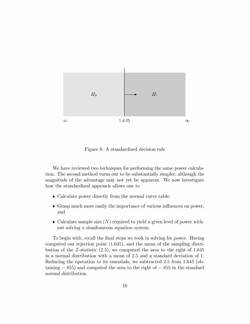
Figure 6: A standardized decision rule

We have reviewed two techniques for performing the same power calcula-tion. The second method turns out to be substantially simpler, although themagnitude of the advantage may not yet be apparent. We now investigatehow the standardized approach allows one to

� Calculate power directly from the normal curve table;

� Grasp much more easily the importance of various in�uences on power,and

� Calculate sample size (N) required to yield a given level of power with-out solving a simultaneous equation system.

To begin with, recall the �nal steps we took in solving for power. Havingcomputed our rejection point (1:645), and the mean of the sampling distri-bution of the Z-statistic (2:5), we computed the area to the right of 1:645in a normal distribution with a mean of 2:5 and a standard deviation of 1.Reducing the operation to its essentials, we subtracted 2:5 from 1:645 (ob-taining �:855) and computed the area to the right of �:855 in the standardnormal distribution.

16

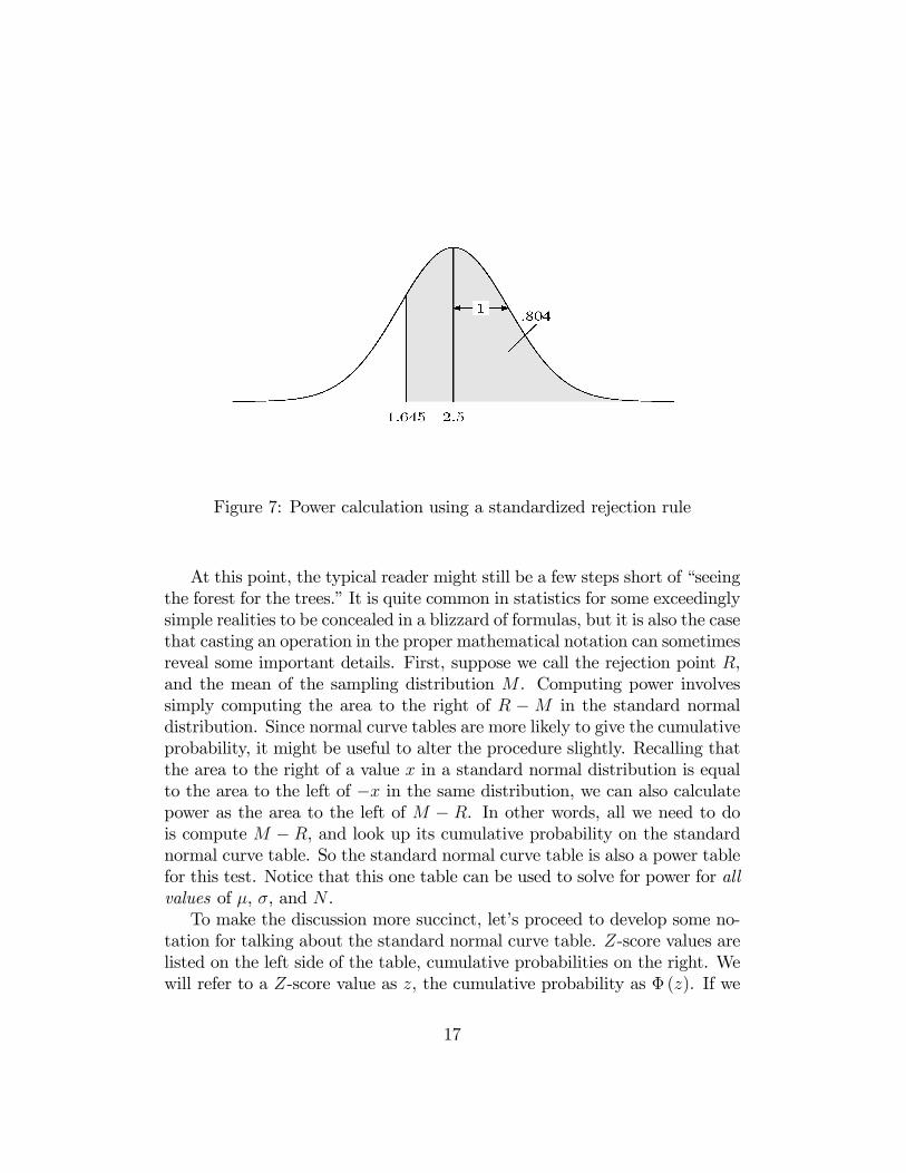
Figure 7: Power calculation using a standardized rejection rule

At this point, the typical reader might still be a few steps short of �seeingthe forest for the trees.�It is quite common in statistics for some exceedinglysimple realities to be concealed in a blizzard of formulas, but it is also the casethat casting an operation in the proper mathematical notation can sometimesreveal some important details. First, suppose we call the rejection point R,and the mean of the sampling distribution M . Computing power involvessimply computing the area to the right of R �M in the standard normaldistribution. Since normal curve tables are more likely to give the cumulativeprobability, it might be useful to alter the procedure slightly. Recalling thatthe area to the right of a value x in a standard normal distribution is equalto the area to the left of �x in the same distribution, we can also calculatepower as the area to the left of M � R. In other words, all we need to dois compute M � R, and look up its cumulative probability on the standardnormal curve table. So the standard normal curve table is also a power tablefor this test. Notice that this one table can be used to solve for power for allvalues of �, �, and N .To make the discussion more succinct, let�s proceed to develop some no-

tation for talking about the standard normal curve table. Z-score values arelisted on the left side of the table, cumulative probabilities on the right. Wewill refer to a Z-score value as z, the cumulative probability as � (z). If we

17

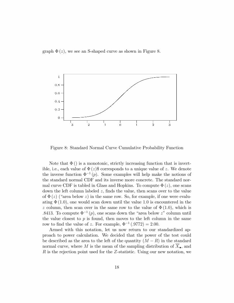
graph � (z), we see an S-shaped curve as shown in Figure 8.

Figure 8: Standard Normal Curve Cumulative Probability Function

Note that � () is a monotonic, strictly increasing function that is invert-ible, i.e., each value of � (z)$ corresponds to a unique value of z. We denotethe inverse function ��1 (p). Some examples will help make the notions ofthe standard normal CDF and its inverse more concrete. The standard nor-mal curve CDF is tabled in Glass and Hopkins. To compute � (z), one scansdown the left column labeled z, �nds the value, then scans over to the valueof � (z) (�area below z) in the same row. So, for example, if one were evalu-ating � (1:0), one would scan down until the value 1:0 is encountered in thez column, then scan over in the same row to the value of � (1:0), which is:8413. To compute ��1 (p), one scans down the �area below z�column untilthe value closest to p is found, then moves to the left column in the samerow to �nd the value of z. For example, ��1 (:9772) = 2:00.Armed with this notation, let us now return to our standardized ap-

proach to power calculation. We decided that the power of the test couldbe described as the area to the left of the quantity (M �R) in the standardnormal curve, where M is the mean of the sampling distribution of X�, andR is the rejection point used for the Z-statistic. Using our new notation, we

18

can write that same quantity as Power = �(M �R) = ��pNEs �R

�.

Since the � () function has an inverse, ��1 (� (x)) = x, and we can actu-ally solve this equation to determine the minimum N required to produce agiven power. Speci�cally, let P be the required power.Then

P = ��pNEs �R

�so

��1 (P ) =pNEs �R

and

N =

���1 (P ) +R

Es

�2Usually N in the above will not be an integer, and to exceed the required

power, you will need to use the smallest integer that is not less than N . Thisvalue is called ceiling(N). Moreover, in a single-sided (1-tailed) test, we canwrite

R = ��1(1� �)So we can make the resulting expression look really complicated! For a

1-sided test such as the one currently under consideration,

N = ceiling

"���1 (P ) + ��1 (1� �)

Es

�2#

Example 5.1 Suppose that the null hypothesis is that � � 70, but the truestate of the world is that � = 75, while � = 10. Find the minimum samplesize needed to achieve a statistical power of :90 when Type I error is set at� = :05.

Solution 5.1 Scanning down the normal curve table we �nd that ��1 (:90) =1:283, and ��1 (1� :05) = ��1 (:95) = 1:645. The standardized e¤ect size is(�� �0)=� = :5. So the minimum N is

N = ceiling

"�1:282 + 1:645

:5

�2#= ceiling [5:854]2

= ceiling[34:27] = 35

19

6 1-tailed and 2-tailed Tests

So far we have examined a situation where the null hypothesis would berejected only on the basis of evidence that the parameter is on one side ofthe acceptance region. In some situations, however, the rejection region istwo sided. The classic case is the null hypothesis of the form � = �0. Avalue of X� far above �0 or far below �0 should result in rejection of thenull hypothesis. Consequently, there will be two rejection regions. Such ahypothesis test is commonly called �two-sided�or �two-tailed.�Commonly, two-tailed tests have symmetric rejection regions in the sense

that half the � is assigned to each tail. One consequence of having a two-tailed test as opposed to a one-tailed test is that the rejection points will bedi¤erent. Consider a test with � = :05. In the 1-tailed version, the rejectionpoint R for the Z-statistic is either 1:645 or �1:645, but not both. In the2-tailed version, the rejection points are both �1:96 and +1:96. The bottomline is that if the null hypothesis is false, and if you run a 1-tailed test withthe rejection region on the correct side, you will have greater power, and asmaller required N , because R will be less.We can revise our formula for required N to take into account T , the

number of tails, as follows

N = ceiling

"���1 (P ) + ��1 (1� �=T )

Es

�2#(4)

The equation for power becomes

P = �hpNEs � ��1 (1� �=T )

i(5)

= �

�pN�� �0�

� ��1 (1� �=T )�

(6)

7 In�uences on Power

By examining Equations 4 and 6 we can see more clearly the factors thatin�uence power, and, in some cases, allow us to manipulate it. Since both� () and ��1 () are strictly increasing in their arguments, it follows thatanything that increases the argument within brackets in Equation 4 willincrease the required sample size, and anything that increases the argument

20

within brackets in Equation 6 will increase power. We will discuss these inclass

1. Sample Size (N)

2. E¤ect Size (�� �0)

3. Variation (�)

4. Type I Error Rate (�)

5. Number of Tails in the Rejection Region (T )

21