hypocenter locations and focal mechanism solutions of
TRANSCRIPT

Hypocenter Locations and Focal Mechanism Solutions of Earthquakes in the EpicentralArea of the 1886 Charleston, South Carolina, Earthquake
Anna Corella Hardy
Thesis submitted to the faculty of the Virginia Polytechnic Institute and State Universityin partial fulfillment of the requirements for the degree of
Master of ScienceIn
Geosciences
Committee Chair: Martin ChapmanJohn HoleYing Zhou
December 5th, 2014Blacksburg, Virginia
Keywords: earthquakes, seismicity, seismic hazard, South Carolina
i

Hypocenter Locations and Focal Mechanism Solutions of Earthquakes in the EpicentralArea of the 1886 Charleston, South Carolina, Earthquake
Anna Corella Hardy
ABSTRACT
The Charleston earthquake of 1886 was one of the largest shocks to occur on the eastern coast of North America. The geological cause has long been a controversial issue and a variety of source models have been proposed. Previous potential field modeling and reinterpretation of seismic reflection and well data collected in the early 1980s indicate that the crust between approximately 1 and 4.5 km depth is comprised primarily of Mesozoic mafic rocks, with extensive faulting that is spatially coincident with modern seismicity in the epicentral area (Chapman and Beale, 2010). This thesis proposes a new and testable hypothesis concerning the fault source of the 1886 shock that is very different from all previous interpretations. It is based on data collected during 2011-2012 from a local seismic network deployment in the immediate epicentral area. The 8-station temporary network was designed to better constrain earthquake hypocenter locations and focal mechanisms. Hypocenter locations of 134 earthquakes indicate a south-striking, west-dipping seismogenic zone in the upper 12 km of the crust. Over 40% of the 66 well-constrained focal mechanisms show reverse faulting on approximately north-south trending nodal planes, consistent with the orientation of the tabular hypocenter distribution.
I offer the following hypothesis: The 1886 shock occurred by compressional reactivation of a major, south-striking, west-dipping early Mesozoic extensional fault. The modern seismicity can be regarded as a long-term aftershock sequence that is outlining the 1886 damage zone. Variability of shallow focal mechanisms is due to the complex early Mesozoic fault structure in the upper 4-5 km.
ii

Acknowledgements
I would first like to acknowledge the funding sources that made this research possible: award number G11AP20141 from the U.S. Geological Survey External Research Program, for the purpose of deploying the seismic network from which my dataset was derived.
I would like to acknowledge many people who have supported me throughout the past couple years. First and foremost, I would like to thank my advisor, Dr. Martin Chapman. He has always made himself available to help, teach, encourage, challenge, and support me, despite his extraordinarily busy schedule. I was fortunate to know him asa professor and research mentor as an undergraduate student, and I have continued to learn much from him as a graduate student. Finally, I want to thank him for his patience and kindness during many difficult challenges I faced in my graduate career, which at times affected my motivation and progress. I would like to extend this gratitude for patience and kindness to my committee members, Dr. John Hole and Dr. Ying Zhou. I also had the pleasure of having them as undergraduate professors, and I am grateful for all they have taught me, both in and out of the classroom. I would like to additionally thank Jake Beale, a research associate at the Virginia Tech Seismological Observatory (VTSO), who has been a great mentor and friend to me during this project.
I would also like to acknowledge the Department of Geosciences as a whole. Thestaff, including the main office administrators, technical support, museum coordinator Llyn Sharp, and especially Connie Lowe, has been a consistent source of support and assistance. In addition to the staff, I am also grateful for all the professors I have had the opportunity to work with and learn from.
I would also like to acknowledge the numerous students, both inside and outside the Department of Geosciences. The students involved in research at the VTSO have been an extremely valuable resource to me throughout the entire project, and I am extremely appreciative of their constant willingness to provide help and research resources to me. The other students in geophysics and in the department have been immensely supportive, and I am thankful for each and every one of them I have gotten to know. I would also like to thank the students and professors at the University of South Carolina for their collaborative research ideas and knowledge of the study region.
Finally, I would like to acknowledge my friends and family, without whom I would not be the person I am today. Their support, love, and encouragement have lifted me during challenging times and have made my life so rewarding every day.
iii

Table of ContentsABSTRACT........................................................................................................................iiAcknowledgements............................................................................................................iiiTable of Contents................................................................................................................ivList of Figures......................................................................................................................vList of Tables......................................................................................................................viList of Abbreviations.........................................................................................................viiChapter 1: Introduction........................................................................................................1
1.1: The 1886 Charleston, South Carolina Earthquake...................................................11.2: Overview of studies related to the 1886 Earthquake................................................21.3: Tectonic setting.........................................................................................................31.4: Modern seismicity in South Carolina.......................................................................51.5: Implications of seismicity.........................................................................................61.6: Project overview.......................................................................................................7
Chapter 2. Data Processing and Methods............................................................................82.1: Data set and station network overview.....................................................................82.2: Processing steps........................................................................................................82.3: Picking phase arrival times, polarities, and amplitudes..........................................11
Chapter 3. Determining hypocenters................................................................................133.1: Locating hypocenters using Hypoellipse................................................................133.2: Re-locating hypocenters using HypoDD................................................................153.3: Plotting and analysis of hypocenters......................................................................183.4: Discussion and implications of results...................................................................20
Chapter 4. Determining focal mechanisms........................................................................224.1: Source characterization using focal mechanisms...................................................224.2: Determining focal mechanisms using Focmec.......................................................244.3: Constraint testing....................................................................................................254.4: Plotting and analysis of focal mechanisms.............................................................264.5: Discussion and implications of results...................................................................27
Chapter 5. Conclusions......................................................................................................28References..........................................................................................................................32Appendix A: Figures..........................................................................................................39Chapter 1:...........................................................................................................................39Chapter 2:...........................................................................................................................45Chapter 3:...........................................................................................................................51Chapter 4:...........................................................................................................................58Appendix B: Tables...........................................................................................................67
iv

List of FiguresChapter 1: 1.1: A diagram showing the Modified Mercalli Intensity (MMI) Scale.............................391.2: A contoured MMI map for the 1886 Charleston, earthquake....................................401.3: A proposed fault model for the study region..............................................................411.4: Detailed maps of the study region..............................................................................421.5: Processed seismic reflection profile VT-3...................................................................431.6: A map of the study region shwoing the magnetic gradient and imaged faults...........44
Chapter 2: 2.1: The seismic network used for the monitoring experiment .........................................452.2: A diagram illustrating the rotation of horizontal station components.......................462.3: A flow chart outlining the processing steps carried out for each station record.......472.4: A diagram comparing raw data and processed data.................................................482.5A: Processed 3-component station record (MTBA) with interpreted wave phases......492.5B: Another example (MTBA) with wave phases and a large converted phase.............492.6: A diagram showing the convention of picking a wave phase.....................................50
Chapter 3:3.1: A diagram showing the 1-D velocity model...............................................................513.2A: Hypocenter locations with Hypoellipse...................................................................523.2B: Hypocenter locations with Hypoellipse: a different perspective.............................533.3A: Hypocenter locations with HypoDD........................................................................543.3B: Hypocenter locations with HypoDD: a different perspective..................................553.4: A diagram summarizing the definition of strike, dip, and rake..................................563.5: A comparison of hypocenter locations from two seismic networks............................57
Chapter 4:4.1: A diagram summarizing the double-couple force system...........................................584.2: A diagram of determining focal mechanisms from P-wave first motions...................594.3: A diagram showing the beachball diagrams for the 3 fundamental fault types.........604.4: Comparison of focal mechanism solutions derived from different data types............614.5: Focal mechanism solutions and constraint tests for an event in the dataset.............624.6: The distribution of the 66 well-constrained focal mechanisms..................................634.7A-E: The focal mechanisms plotted with the events relocated using HypoDD...........64
v

List of TablesTable 1: Network information...........................................................................................67Table 2: Polarity conventions for each phase...................................................................67Table 3: Ph2dt parameters.................................................................................................67Table 4: HypoDD parameters...........................................................................................68Table 5: Focmec parameters.............................................................................................68Table 6: Rating system......................................................................................................68Table 7: Summary of Focal Mechanism Results..............................................................69
vi

List of Abbreviations
km: kilometers
Hz: Hertz
SGR: South Georgia Rift
Mw: Moment Magnitude; A measure of earthquake size, based on the static seismic moment of an earthquake.
MMI: Modified Mercalli Intensity; A measure of earthquake size, based on shaking and damage.
Md: Duration Magnitude; A measure of earthquake size, based on the duration of an earthquake, correlated with mb(Lg).
mb(Lg): Body Wave Magnitude based on the Lg phase; a measure of earthquake size, designed to be numerically identical with the teleseismic mb scale. This measure is commonly used for earthquakes in the central and eastern U.S recorded at regional distance.
P: Primary wave.
S: Secondary or Shear wave.
SH: Horizontal component of the shear wave.
SV: Vertical component of the shear wave.
Vp/Vs: The ratio of P wave velocity (Vp) to S wave velocity (Vs).
SEH: Standard Horizontal Error; confidence limit in the least-constrained horizontal direction.
SEZ: Standard Vertical Error; confidence limit in the vertical direction (depth).
RMS: Root Mean Square.
SVD: Singular Value Decomposition; A weighted least squares inversion method.
LSQR: conjugate gradients method; A weighted least-squares inversion method.
SEUSSN: South Eastern United States Seismic Network.
vii

Chapter 1: Introduction
1.1: The 1886 Charleston, South Carolina Earthquake
At 9:51 PM local time on August 31, 1886 a major earthquake occurred
beneath the then small village of Summerville, South Carolina. It is one of the largest
earthquakes to occur on the East Coast of North America, with recent moment
magnitude (Mw) estimates in the range 6.4 to 7.3 (Johnston, 1995; Bakun and Hopper,
2004). It is by far the worst earthquake disaster to have occurred on the eastern
seaboard of the United States. Damage in the epicentral area reached X on the
Modified Mercalli Intensity (MMI) scale (Bollinger, 1977). A value of MMI X
represents severe damage and extreme shaking (Figure 1.1). Serious damage occurred
in Charleston, South Carolina approximately 30 km from the epicenter where at least
83 people were killed either directly or indirectly as a result of injury and exposure
(Dutton, 1889). A contoured map of the MMI from this earthquake shows the extent
of the reports of felt shaking (Bollinger, 1977) (Figure 1.2).
Prior to the 1906 San Francisco earthquake, the Charleston event was the most
significant earthquake disaster in the United States. This earthquake occurred in a
period of time in which earthquake seismology was still a young science and no
seismographic recordings were available; therefore the existing data were derived
from observations of damage to structures and ground failure, such as liquefaction
and lateral spreading, as well as personal accounts from people that experienced the
earthquake. These observations were compiled in the 9th annual report of the USGS by
Captain Clarence Dutton (Dutton, 1889). The earthquake occurred in the Atlantic
coastal plain, where sediments are approximately one km in thickness. No conclusive
evidence for faulting was observed in 1886. The geologic cause of the earthquake
remains a matter of debate, and is the subject of this thesis.
1
1.2: Overview of studies related to the 1886 Earthquake
This section provides a brief overview of the previously proposed source
mechanisms of the 1886 earthquake. The earliest interpretation is based on the
shaking effects observed mostly along three railroads and was put forth soon after the
earthquake by Clarence Dutton and a local geologist, Earle Sloan. Both Dutton and
Sloan interpreted the main shock to have multiple epicenters (Dutton, 1889). In the
years following the publication of the Dutton (1889) report, many researchers have
attempted to build on this interpretation and propose fault models for the region.
Taber (1914) studied the intensity data near Summerville and proposed a northeast-
trending fault source of the 1886 earthquake that he referred to as the Woodstock
Fault. USGS professional papers compiled the results of various studies undertaken
by many researchers (Rankin, 1977; Gohn, 1983). Tarr (1977) suggested that the
earthquakes detected near Summerville by a permanent seismic network installed in
1974 were closely associated with the rupture of the main shock. Long and
Champion (1977) suggested that the shock was the result of local stress amplification.
Seismic reflection profiles collected in the 1970’s and early 1980's revealed several
minor Cenozoic faults with reverse slip sense that could be associated with the local
seismicity and the 1886 earthquake (Hamilton et al., 1983; Yantis et al., 1983;
Chapman and Beale, 2008; 2010). A series of papers by Madabhushi and Talwani
(1993), Dura-Gomez (2004), Dura-Gomez and Talwani, (2009) developed a fault
model based largely on hypocenter locations of earthquakes occurring between 1974
and 2004. That model consists of a proposed Southwest-striking, Northwest dipping
strike-slip fault (Woodstock fault), approximately 50 kilometers in length, with a
compressional step-over (Sawmill Branch fault) near Middleton Place (Figure 1.3).
Chapman and Beale (2008; 2010) reprocessed seismic profiles and modeled the
2

potential field. Their work indicates that the crust between 1 and 5 km depth in the
epicentral area of the 1886 shock is comprised largely of mafic material, and
discovered that the modern instrumentally located seismicity is in close proximity to
at least four imaged faults that represent Cenozoic compressional reactivation of early
Mesozoic extensional faults at shallow crustal depths (Figure 1.6).
1.3: Tectonic setting
The epicentral region of the 1886 earthquake is located within a large
extensional terrain referred to as the South Georgia Rift (SGR) or the South Georgia
Basin. This terrane was associated with the initial rifting of the supercontinent
Pangaea that led to the formation of the Gulf of Mexico and the Atlantic Ocean
beginning in the Triassic period. The region is overlain by Atlantic Coastal Plain
sediments. Previous studies indicate that the lithology of the terrane is characterized
by mafic volcanics, largely basalt, and clastic red-bed sediments similar to those
found in exposed Triassic basins in the Appalachian region (Gohn 1983, McBride
1991). The geologic structure of the SGR is not well resolved, but potential field
modeling done by Chapman and Beale (2010) indicates that the mafic material
extends to at least four km depth in the Summerville area.
In addition to potential field modeling, there are also several wells within the
region. Three wells near Clubhouse Crossroads, located a few kilometers southwest of
Summerville (Figure 1.4), all encountered basalt immediately below Cretaceous
coastal plain sediments. Only one out of the three Clubhouse Crossroads wells
penetrated through the basalt layer, and it bottomed within a package of sedimentary
red beds at a depth of 1,140 m (Gohn, 1983). An exploratory well near Lodge, South
Carolina, about 70 km west of Summerville (Figure 1.4), penetrated alternating layers
3

of mafic volcanics and sediments and bottomed out in basalt at 3.8 km (Talwani,
2000). From these data, it is inferred that the lithology and structure of the SGR is
complex and that the sequence of early Mesozoic mafic volcanics and clastic
sediments is locally several kilometers thick, particularly in the Summerville area.
Seismic reflection profiles, collected in the late 1970's and early 1980’s by the
United States Geological Survey (USGS), the Consortium for Continental Reflection
Profiling (COCORP), and Virginia Tech (VT) reveal much about the localized
tectonic setting of the epicentral region. The seismic lines are shown with respect to
the local county lines and rivers (Figure 1.4). There are several prominent bright
reflectors seen in the lines, which represent a change in seismic impedance.
Impedance is a seismic property, related to both the density of the rock and the
seismic wave velocity. Changes in seismic impedance are due to compositional
differences of the lithology in the subsurface. The most prominent reflectors are
labeled K, J, and B (Figure 1.5). The B reflector was originally interpreted as the top
of crystalline basement (Hamilton et al., 1983), but with the evidence from gravity
and magnetic modeling (Chapman and Beale, 2010), and the Lodge well, it has since
been reinterpreted as a basalt layer (Chapman and Beale, 2010). The J reflector is
interpreted to be an unconformable contact between the early Jurassic basalt and red
beds and the Cretaceous Atlantic coastal plain sediments that overly it. This reflector
is strong in some profiles, particularly in line VT-3b, and weak in others. Near
Clubhouse crossroads, the J reflector is clearly due to the basalt unit encountered in
wells at the base of the coastal plain sediments. The J reflector changes character in
different parts of the study area, and appears to be missing altogether in some places
(Buckner, 2011), but it has been explained as locally homogenous material, in some
places yielding a weak seismic impedance contrast (Chapman and Beale, 2008; 2010).
4

The K reflector is interpreted as the contact between Cretaceous and Cenozoic coastal
plain sediments.
The seismic profiles obtained in the SGR reveal a complex system of
extensional structures in the region (McBride, 1991). In the study area near
Summerville, the B reflections show down-to-the-east offset consistent with
extensional faulting; however the reflection profiles also show evidence of Cenozoic
compressional reactivation of these faults. Cenozoic offset is most prominently seen
in line VT-3b (Figure 1.5), as minor offset of the J and shallower reflectors. Evidence
of Cenozoic faulting on other reflection profiles consists of monocline folding of the
Cenozoic sediments above early Mesozoic fault offsets. Evidence for this faulting is
also seen in the magnetic modeling by a steep magnetic gradient of the total intensity
magnetic field. The seismic reflection profiles that pass over this gradient all exhibit
Cenozoic deformation at that location (Figure 1.6).
1.4: Modern seismicity in South Carolina
The record of historical seismicity near Charleston and Summerville suggests
activity both prior to and after the 1886 earthquake (Rankin 1977; Bollinger and
Visvanathan, 1977). Paleo-liquefaction data indicates that several events, similar in
magnitude to the 1886 earthquake, have occurred with an approximate recurrence rate
of 500-600 years (Talwani and Schaeffer, 2001). Rankin (1977) suggested that recent
seismicity represents aftershocks from the 1886 earthquake or events associated with
the activation of closely related structures due to the change in the stress field caused
by the 1886 shock. The complete historical catalog of earthquakes for South Carolina,
beginning in 1698, has been compiled from a variety of sources. The events prior to
the 1886 earthquake have been compiled into the catalog primarily from newspapers
5

and public observation reports (Bollinger and Visvanathan, 1977). Since the 1886
earthquake, many efforts have been made to improve and update this catalog.
In 1914, six earthquakes were recorded near Charleston, as well as two in the
Piedmont region of South Carolina. MMI values were estimated for these
earthquakes, and ranged between II and V (Taber, 1915). In 1973, a seismic network
of 10 stations was installed in the region in an effort to monitor the regional
seismicity. Between May 1974 and December 1975, approximately 75 earthquakes
were detected, with duration magnitudes (Md) ranging between 1.5 and 3.8 (Tarr,
1977). The catalog was updated by Tarr and Rhea (1983), compiling the events
detected between March 1973 and December 1979 with a larger seismic network
consisting of 21 stations. During this time, approximately 60 events were recorded,
with Md ranging from 0.6 to 3.8; the majority of the events were located near
Summerville. Beginning in 1974, a permanent seismic network has been deployed
near Summerville, South Carolina, and is currently operated by the University of
South Carolina.
1.5: Implications of seismicity
The historical seismic record indicates that the study area is one of the more
seismically active regions in the eastern United States. An earthquake comparable to
the 1886 earthquake would be catastrophic. Wong et al. (2005) conducted a
comprehensive earthquake loss assessment for South Carolina, using Mw = 7.3
earthquake near Summerville as the seismic source. They used federal government
loss estimation software known as HAZUS 99, to estimate the spatial extent and
scope of structural damage, casualties, and economic loss for the earthquake scenario.
The results indicated that there would be approximately 45,000 casualties, 900 of
6

which would be fatalities. Extensive structural damage would result in losses of over
14 billion USD (estimate in 2000).
The results of Wong et al. (2005) also indicate that a significant percentage of
the state’s lifelines, such as hospitals and fire stations, would have moderate to severe
damage. Recovery efforts would also be hindered, due to severe damage of
approximately 800 bridges. It is noted that there were several uncertainties in the
parameters used to determine the losses, particularly with the ground shaking
estimates; however, the results still shed light on the severity of the potential
earthquake risk, as well as emphasizing the need for risk mitigation. Understanding
the seismicity of the region is essential for better-constrained estimates of the ground
shaking associated with regional seismic events, which are crucial for the on-going
earthquake risk mitigation efforts in South Carolina.
1.6: Project overview
The purpose of this study is to shed more light on the modern seismicity near
Summerville, to determine the likely fault(s) associated with the earthquake, and
develop a testable hypothesis for the geologic process driving the 1886 earthquake.
The study involves analysis of data collected in a one-year seismic monitoring
experiment. The results of the data analysis are accurate hypocenter locations and
well-constrained focal mechanism solutions, which have implications for the causal
fault structure and state of stress associated with the 1886 earthquake.
7

Chapter 2. Data Processing and Methods
2.1: Data set and station network overview
From August 7, 2011 to August 30, 2012, a network of eight temporary
stations funded by the USGS (under award number: G11AP20141: "Experiment to
Determine Hypocenters and Focal Mechanisms of Earthquakes Occurring in
Association with Imaged Faults near Summerville, South Carolina”) were deployed
near Summerville, South Carolina (Figure 2.1; Table 1) to continuously record local
seismicity (Chapman and Beale, 2013). Data were recorded using 3-component, short
period, 2 Hz seismometers (Sercel L-22) on high-resolution digital data recorders
(REF TEK 130), loaned by the IRIS/PASSCAL instrument center at the New Mexico
Institute of Mining and Technology in Soccoro, New Mexico. The stations were
equipped with solar panels to provide power to 12-volt marine storage batteries and
GPS receivers for location and timing. The data were collected with a sample rate of
100 samples/second. The data are archived at the IRIS Data Center under the ‘XY’
seismic network code, and are available to the research community from the IRIS data
management center. In addition to the temporary deployment, 3 permanent seismic
stations supported by the ANSS (Advanced National Seismic System under the
USGS) and operated by the University of South Carolina collected data for the
duration of the experiment (Figure 2.1; Table 1).
2.2: Processing steps
Most of the processing was conducted using the Seismic Analysis Code (SAC)
software package (Goldstein and Snoke, 2005). Through an automated process, the
program read in the data for a given station, synchronized the record start time on all
three components, removed a linear trend, and applied a Butterworth bandpass filter
8
with 3 poles and corner frequencies at 1 and 40 Hz (Figure 2.3). The bandwidth of
the Butterworth filter was less broad for station NHSC (with corner frequencies at 1
and 15 Hz), because of the low Nyquist frequency (20 Hz) for that station.
Synchronizing the data ensures that the signal of all three components begins at the
same reference time. Removing the trend is a signal correction command that
eliminates potential signal slope artifacts when integrating the record; it also
effectively removes the mean amplitude from the data. The Butterworth bandpass
filter preserves the signal amplitude between the two corner frequencies while the
remaining frequencies are reduced in amplitude.
Each recorded component was integrated from the raw signal (proportional to
ground velocity at frequencies greater than 2 Hz) to approximate the single-sided
displacement pulses at the source, thus simplifying the measurement of P and S wave
arrival amplitudes. An ideal displacement phase arrival (either P or S wave) would
consist of a single-sided waveform, in a homogeneous whole space. Integrating the
recorded trace from the 2-Hz velocity sensors used in this study gives a good
approximation to this signal for the small magnitude events of the study region.
An essential step in the data processing was the rotation of the horizontal
components to the radial and transverse directions. This rotation was performed for
two reasons: 1) To allow accurate S wave arrival time picking from the transverse
component, and 2) to isolate the SV and SH components of the S wave for amplitude
measurement. This step in the processing required an initial estimate of the
hypocenter location in order to determine the source-receiver azimuth needed to
establish the radial and transverse component directions.
Over the course of the monitoring experiment, 134 locatable earthquakes were
identified in the data set. P and S-wave arrival times were picked on the un-rotated
9

components and the hypocenters were initially located individually using the
computer program Hypoellipse (Lahr, 1999). Given the source-receiver azimuth
estimates from the initial location, the rotation of the North-South and East-West
components to transverse and radial horizontal components was done using Equation
1, implemented by SAC (Figure 2.2).
[RT ]= M2D [ N
E ] ; M2D = [cos(a) sin(a)-sin(a) cos(a) ] . (1)
The variable, a, represents the azimuth measured clockwise from North, which was
determined in the initial Hypoellipse location. Two permanent stations (CSB and
RGR) have been installed in boreholes with undetermined orientation of the
horizontal components. As a consequence, rotation was not implemented for CSB and
RGR, and SV and SH polarity and amplitude measurements could not be made for
those stations.
Following the initial location of the hypocenters, and creation of transverse
and radial components of motion, a coda duration magnitude for each event was
calculated using Equation 2, developed by the Virginia Tech Seismic Observatory,
which is calibrated to the body wave magnitude scale (mb(Lg)). Several network
operators in the southeastern United States have used this duration magnitude since
the early 1980's (M. C. Chapman, personal communication).
MD = -3.42+2.83 Log D (2)
The duration magnitudes of the earthquakes ranged from -1.8 to 2.6. Figure 2.4
shows a comparison of unprocessed versus processed seismograms. After processing,
the signal to noise ratio was improved, and the P and S-wave arrivals appear more
impulsive and easier to distinguish.
10

2.3: Picking phase arrival times, polarities, and amplitudes
After the processing described above, the data were extensively analyzed to
identify and measure body wave arrival times, polarities and amplitudes: the P wave
on the vertical component, the SH component of the S wave on the transverse
component, and the SV component of S wave on the radial component. Figure 2.5a
shows an example seismogram from the dataset, with the interpreted arrival times for
each phase. Noise and the presence of converted energy complicated this process. In
a general sense, converted waves result from scattering due to velocity and density
heterogeneities in the Earth (M. C. Chapman, personal communication). This
scattered energy is present in the seismograms, in addition to the direct P and S
arrivals, making it more difficult to interpret the direct P and S arrivals. Conversion
of SV to P waves was a particular problem for the radial component. The S to P
converted phase due to the velocity contrast at the base of the coastal plain
sedimentary section can have large amplitudes on the vertical and radial components.
Figure 2.5b shows an example from the data set where the converted phase is very
prominent. This phase can easily be mistaken for the SV arrival, and it takes an
experienced eye and 3-component data to distinguish the two. S to P conversion at
other points along the raypath can also generate precursory arrivals that further
complicate the measurement of SV arrival time and amplitude. For this reason, the
SH arrival times derived from the transverse components were used to establish the S
wave arrival times necessary for final hypocenter location. A weight, ranging between
0 and 4 was assigned to each P and S arrival time to characterize the quality and
uncertainty associated with the picks. In Hypoellipse, a weight of 0 is assigned to a
phase arrival if it is fairly impulsive and easy to distinguish from surrounding noise,
while a weight of 4 is assigned if there is no discernable wave phase arrival in the
11

record. In practice, arrivals were assigned with weights of 0, 2, and 4 for consistency.
Weighting is an integral part of picking P and S arrival times, as it is used in part to
determine the uncertainty of earthquake locations (Chapter 3).
In addition to the arrival times, the polarity and amplitude of each direct body
wave phase was picked using the first half-cycle of motion following the arrival onset,
and were recorded using SAC (Figure 2.6). P-wave arrival times, polarities and
amplitudes were determined using the vertical component. S wave arrival time, SH
polarities and amplitudes were determined using the transverse horizontal component.
SV polarities and amplitudes were determined from the radial horizontal component.
The naming convention for P wave polarity is U or D for either first motion in the up
or down direction. The SH polarity naming convention is R or L, corresponding to
first motion to the right or left, when looking in the direction of source-to-receiver
azimuth. The convention for SV is F or B, representing either forward (horizontal
motion away from the source) or backward (horizontal motion toward the source)
along the source-to-receiver azimuth (Table 2). The phase amplitudes corresponded to
either the amplitude of the first peak or trough following the phase arrival time,
measured in digital counts on the integrated seismograms.
12

Chapter 3. Determining hypocenters
3.1: Locating hypocenters using Hypoellipse
All events in the data set were initially located using a computer program
called Hypoellipse (Lahr, 1999). Hypoellipse determines the hypocenter of regional
earthquakes. The hypocenter is the location at depth of earthquake rupture initiation,
whereas the epicenter is the projection of the hypocenter on the surface of the Earth.
Hypoellipse uses Geiger’s method for earthquake location, which involves the
linearization of a nonlinear problem, as the relationship between P and S arrival times
and the spatial location of an earthquake, is nonlinear (Lahr, 1999; Waldhauser, 2001).
The resultant linear relationship relates travel-time residuals to perturbations in a
given earthquake location model containing spatial and temporal parameters
(Waldhauser and Ellsworth, 2000).
Hypoellipse implements the weighted Least Squares inversion method to
effectively minimize the root mean square (RMS) of the residual of observed and
calculated travel-times from source to station through an iterative process (Lee and
Dodge, 2010). A solution for the location model is achieved after several iterations,
containing spatial x-y-z coordinates of the source and a source origin time, as the
RMS of the travel-time residual is minimized to a reasonable user-defined value.
Equation 3 shows the equation for the travel-time residual below, where the observed
travel-time is known through the P and S arrival times and the calculated travel-time
is theoretical and based upon the velocity model used for the region. Equation 4
shows the root mean square residual for iterations 1 through N, where i is a given
iteration, and W is the weight computed by Hypoellipse for the i’th iteration (Lahr,
1999).
13

ri = ( τobs - τcalc ) (3)
RMS = √∑1
n
W i r i2
∑1
N
W i
(4)
Several parameters must be defined to control the execution of Hypoellipse.
Most of these parameters control the weighting of the data as iteration progresses. The
fundamental user-provided inputs to the program are the phase arrival times, seismic
station locations and an appropriate 1-dimensional velocity model. The user can also
provide initial estimates of the hypocenter and/or origin time. The P and S arrival
times were measured from the seismograms collected in the study area (see Chapter
2). The velocity model is needed to determine the theoretical travel times, used to
calculate the residual in equation 3. A velocity model previously determined
consisting of three layers over a half-space, was used for this analysis (Chapman et
al., 2003). The velocity model (Figure 3.1) incorporated a shallow layer representative
of the Cretaceous and younger coastal plain sediments, with P and S wave velocities
2000 km/s and 0.667 km/s respectively. The second layer contained higher P and S
wave velocities of 6000 km/s and 3.468 km/s respectively, representative of the lower
Mesozoic volcanic and sedimentary rock section. The third layer, representative of the
deeper crust contained somewhat higher P and S wave velocities, 6.5 km/s and 3.757
km/s respectively, that were determined from refraction velocity measurements in the
Piedmont province of Virginia (Bollinger et al., 1980). Due to the small epicentral
distances involved in this study, only the two shallowest layers are important.
134 earthquakes in total were located using Hypoellipse, and the resultant
hypocenters are shown in both map view and in two perspective views (Figure
14
3.2a,b). When looking along an approximate East-West cross-section slice, the
hypocenters appear to define a tabular zone trending approximately North-South and
dipping towards the west. The implications of this result will be discussed further in
Chapter 5.
For each hypocenter, Hypoellipse also determines a 68% confidence limits of
the location, defined by SEH and SEZ, the horizontal and vertical semi-major axes of
an ellipsoid representing the confidence limit in the least well-constrained horizontal
direction and the confidence limit at depth, respectively (Lahr, 1999). These errors are
based upon an estimated standard error of arrival times calculated by the program, the
weight code assigned to each arrival time, and the partial derivative of travel-time
from the source to each station. The standard error of arrival times is either computed
by Hypoellipse, on the basis of the RMS residual or set by the user at an appropriate
fixed value. In the case of small data sets, significant uncertainties in the locations of
the hypocenters can result from arrival time reading the errors and poor spatial
constraint. In addition, uncertainties in the velocity model can lead to bias in the
locations. Under the right conditions, relative location methods can be used to greatly
reduce the effects of error in the velocity model. This approach was used to good
advantage in this study, as described below.
3.2: Re-locating hypocenters using HypoDD
Hypocenter locations are often relocated relative to each other to yield more
precise relative locations. A computer program known as HypoDD implements a
double-difference location algorithm, and was used to relocate the earthquake
hypocenters determined by Hypoellipse. Like Hypoellipse, HypoDD linearizes the
nonlinear relationship between the source location and its station arrival times using
15

Geiger’s method, but minimizes the differences in travel-time for two nearby events
(Waldhauser, 2001). This residual, referred to as the double-difference, is shown in
Equation 5 (Waldhauser and Ellsworth, 2000):
d rkij = ( t k
i - tkj )obs - ( tk
i - t kj )calc (5)
The index notation is the same as in equation 3, with the addition of index j, which
represents the second event in the earthquake pair. HypoDD gives the option of
minimizing the residuals by weighted least squares with either the Singular Value
Decomposition (SVD) method or by the conjugate gradients (LSQR) method
(Waldhauser, 2001). Both methods have their advantages, based on the goal and
parameters of a given study, but in general SVD is more appropriate for well-
conditioned and smaller clusters of events and the LSQR method is able to efficiently
solve large and potentially ill-conditioned systems (Waldhauser, 2001). While the size
of this dataset is more appropriate for SVD, the LSQR inversion method was used
based on the uncertainty of the condition, due to sparse station coverage. It is noted
that in future work, SVD should be used to invert for the model solution to be
compared with results using LSQR.
As a further constraint, HypoDD allows multiple data input sources to be used
by the program; these include traditional arrival time catalogs comprised of traditional
arrival time picks as described in section 2.3, and/or high precision relative arrival
times determined from cross-correlation waveform data (Waldhauser, 2001). For this
study, the input data source included only catalog data (manual P and S wave arrival
measurements). Waveform cross correlation can provide more accurate relative arrival
time measurements in many cases. However, tests have shown that the small
hypocenter distances and high frequency content seismograms used in this study
16

make for manual arrival time picking accuracy of the same order as that from
waveform cross-correlation.
The first step for earthquake relocation using HypoDD involves data
preparation, performed by a program named ph2dt. The purpose of this program is to
search the catalog data and/or waveform data and link neighboring earthquakes into a
pair and calculate the double-difference for the pair (Waldhauser, 2001). There are
several parameters involved in running this program, which can be altered
appropriately, depending on the dataset. These include the maximum event separation
for linkage, the range of double-difference observations, the maximum amount of
neighboring events, the minimum amount of links for each event, and the maximum
distance between hypocenters, which defines the size of the earthquake cluster. The
parameter values were chosen based on appropriate values for a relatively small event
cluster given by the HypoDD manual (Waldhauser, 2001), and are summarized in
Table 4. In this step, it is possible that events get “thrown out” of the dataset, if they
are defined as outliers to the dataset. Outliers are defined as events containing delay
times that are larger than the maximum expected delay time for a P and S wave to
travel between two events in an event pair. In this study, 47 events were thrown out,
leaving 87 to be relocated.
In the second and final step for earthquake relocation, HypoDD is run to
determine the double-difference hypocenter locations in an iterative process. After
each iteration, the vector difference between nearby hypocenter pairs is adjusted, the
model parameters are updated, and the dataset is weighted based on the data misfit
from inversion. The number of iterations is dependent on the inversion parameters
and the amount of uncertainty within the dataset. A solution is found once the shifts in
hypocenter locations are within the average error of the initial locations or when the
17

RMS residual is minimized to below the threshold of noise in the dataset (Waldhauser,
2001). Many parameters are involved in HypoDD, including the 1-D velocity model,
the Vp/Vs ratio, and the maximum distance between hypocenters. As with ph2dt,
these parameters were also tested with several values to assess their control on the
hypocenter locations, particularly the depths. The only parameter that affected the
depths significantly was altering the Vp/Vs ratio, which illuminates a major limitation
in HypoDD. Only one Vp/Vs ratio can be specified for the entire velocity model,
which is not appropriate for the near-surface depths involved in this study. In Fall
2014, a new version of HypoDD will become available to correct this limitation, and
future work should include multiple Vp/Vs ratios to test the constraint on the
hypocenter depths. The parameters used for HypoDD are summarized in Table 5.
Out of the 134 events, 87 were relocated, and the results are plotted in both
map view and in perspective views in Figure 3.3. When compared to the initial
locations performed by Hypoellipse, the HypoDD algorithm was successful in
tightening the clusters of events, making them more precise. They exhibit the same
North-South trending, west-dipping seismogenic feature observed in the Hypoellipse
locations.
3.3: Plotting and analysis of hypocenters
HypoDD outputs the event re-locations in the format of latitude, longitude,
and depth. Latitude and longitude are used to plot the hypocenters in map view as
epicenters. Viewing hypocenters in perspective plots is advantageous for determining
any geometric trends: e.g., a planar arrangement of hypocenters might represent a
fault. In order to plot them in a perspective view, a reference origin in Cartesian
coordinates (x, y, z) must be determined, as latitude and longitude cannot be used. It is
18

noted here that z is equal to the depth and remains unchanged. The origin of the x-y
coordinate systems is referenced to the mean latitude and longitude of the earthquake
epicenters. Equations 6-8 were used to determine the Cartesian x and y coordinates of
the hypocenters relative to the origin (Bullen and Bolt, 1985):
cos ∆ =A A' + B B' + CC' , (6)
A = sinθ cosϕ, B = sinθ sinϕ, C= cosθ, D = sinϕ, E = -cosϕ (7)
2+ 2 sinΔ sinZ = ( A ' - D)2 + ( B' - E)2 + C'2 , (8)
The variables θ and ϕ represent the mean colatitude and mean longitude of the
epicenter cluster, respectively, and θ ' and ϕ' are the colatitude and longitude of
a given event epicenter, respectively. The angular epicentral distance, between the
origin and epicenter in degrees subtended at the center of a sphere is represented by
∆ , and Z is the azimuth from origin to epicenter in degrees, reckoned East of
North. Cartesian coordinates, x and y in kilometers, with respect to the origin are
given by Equation 3.7.
x = 111.199 Δ sinZ , y = 111.199 Δcos Z . (9)
The HypoDD relocated hypocenters appear consistent with the hypocenters
located with Hypoellipse. In a geologic sense, the orientation of a plane, or a fault, is
defined by a strike and a dip. The strike is defined as the azimuth of a line that marks
the intersection of a given plane with a reference horizontal plane, and the dip is the
acute angle between the plane and the horizontal: positive dip direction is reckoned to
the right when looking in the strike direction (Figure 3.4). A plane was fit to the
hypocenters by weighted least squares for the purpose of quantifying the orientation
of the feature. Hypocenters at depths greater than 7 km were given four times the
weight of the remaining hypocenters. The orientation of the best-fit plane to the
19
hypocenter locations was found to be striking N186E and dipping 43 degrees to the
west. Two additional planes were fit to the HypoDD hypocenter data: 1) with equal
weighting of all events and 2) excluding all hypocenters at depth greater than 7.0 km.
Equal weighting of all events resulted in a least-squares strike of N185E and a dip of
34 degrees, while the exclusion of deeper hypocenters resulted in a strike of N184E
and a dip of 18 degrees. The resultant orientations for the planes included
significantly shallower dips, but the strike of both scenarios was relatively unchanged
(N185E).
3.4: Discussion and implications of results
The 134 hypocenters located with Hypoellipse illuminate a distinct North-
South trending, west-dipping seismogenic zone when viewed in a perspective plot
looking towards the North (Figure 3.2a). HypoDD relocated 87 of the hypocenters,
and they show more consistent and precise relative locations, compared to the
Hypoellipse locations (Figure 3.3a). Most of the events are located within the upper 6
km, and there is a noticeable gap in the trend at a depth of around 8 km. The events
below 8 km are assumed to be significant in conjunction with focal mechanism
solution results (Chapter 4).
The hypocenters discussed above were compared to hypocenters computed for
earthquakes that occurred from 1974-2005. The arrival time data for those earlier
earthquakes were contributed to the Southeastern United States Seismic Network
Bulletins (e.g., Chapman et al., 2006) by Dr. Pradeep Talwani and co-workers at the
University of South Carolina. Those earlier earthquakes were re-located by Jake Beale
and Qimin Wu using the procedure described in detail in the previous sections. The
results indicate good agreement between the two datasets in terms of the plane
20

orientation (Figure 3.5). This is a significant result, as it shows that the hypocenter
results from a one-year monitoring experiment are representative of the longer-term
seismicity during the past 3 decades.
21

Chapter 4. Determining focal mechanisms
4.1: Source characterization using focal mechanisms
A common practice associated with analyzing the seismicity of a region is to
determine the focal mechanism for earthquakes in conjunction with locating
hypocenters. The focal mechanism of a tectonic earthquake is assumed to be
represented by two orthogonal force systems, known as a double couple (Figure 4.1).
The general seismic source is characterized by a seismic moment tensor, in which the
tensor elements represent force couples acting at a point in a continuum. The double
couple is a subset of general seismic moment tensors that represents the force system
responsible for shear dislocation on a plane. It is assumed here that moment tensors of
all the events are pure double couple (Lay, T. and Wallace, T., 1995). In future work, it
would be interesting to derive the general seismic moment tensor, but such work is
beyond the scope of the present study. The double couple focal mechanism can be
described by static moment (or moment magnitude), the strike and dip of the two
nodal planes, and the rake (direction of slip) on the nodal planes. Because of
symmetry, there are two orthogonal nodal planes, either of which could correspond to
the actual fault plane. Determination of which of the two nodal planes is the actual
fault plane requires information in addition to recordings of the far-field seismic
waves. The additional information is usually, as here, furnished by the hypocenter
locations of aftershocks, or in some cases, by geodetic data or by surface rupture.
The standard lower hemisphere stereographic projection of the two nodal
planes is used here to illustrate all focal mechanism solutions. It is constructed with
the orientation of a fault in terms of strike, dip, and rake (Figure 3.4). The rake angle
refers to the direction of slip of the hanging wall of a fault, with respect to the foot
wall. It is reckoned as counterclockwise from the strike direction in the plane of the
22
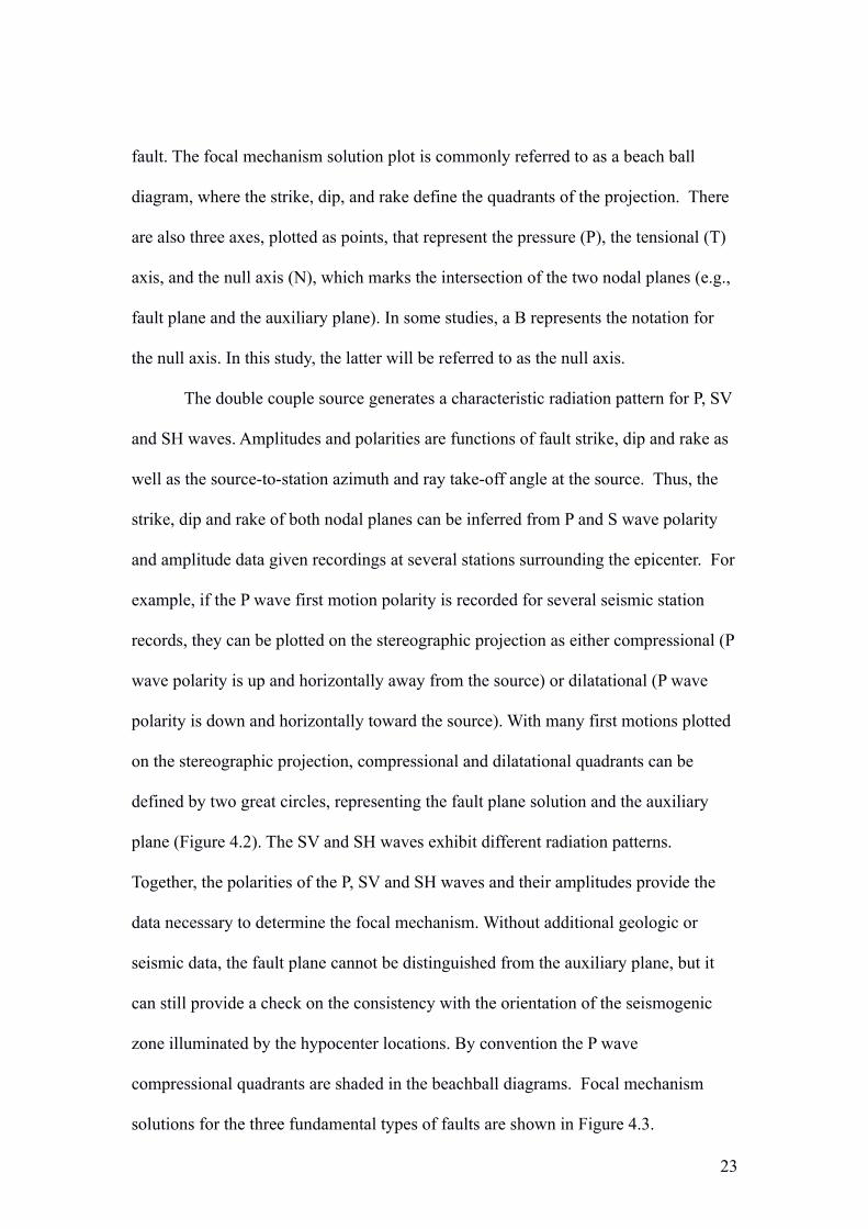
fault. The focal mechanism solution plot is commonly referred to as a beach ball
diagram, where the strike, dip, and rake define the quadrants of the projection. There
are also three axes, plotted as points, that represent the pressure (P), the tensional (T)
axis, and the null axis (N), which marks the intersection of the two nodal planes (e.g.,
fault plane and the auxiliary plane). In some studies, a B represents the notation for
the null axis. In this study, the latter will be referred to as the null axis.
The double couple source generates a characteristic radiation pattern for P, SV
and SH waves. Amplitudes and polarities are functions of fault strike, dip and rake as
well as the source-to-station azimuth and ray take-off angle at the source. Thus, the
strike, dip and rake of both nodal planes can be inferred from P and S wave polarity
and amplitude data given recordings at several stations surrounding the epicenter. For
example, if the P wave first motion polarity is recorded for several seismic station
records, they can be plotted on the stereographic projection as either compressional (P
wave polarity is up and horizontally away from the source) or dilatational (P wave
polarity is down and horizontally toward the source). With many first motions plotted
on the stereographic projection, compressional and dilatational quadrants can be
defined by two great circles, representing the fault plane solution and the auxiliary
plane (Figure 4.2). The SV and SH waves exhibit different radiation patterns.
Together, the polarities of the P, SV and SH waves and their amplitudes provide the
data necessary to determine the focal mechanism. Without additional geologic or
seismic data, the fault plane cannot be distinguished from the auxiliary plane, but it
can still provide a check on the consistency with the orientation of the seismogenic
zone illuminated by the hypocenter locations. By convention the P wave
compressional quadrants are shaded in the beachball diagrams. Focal mechanism
solutions for the three fundamental types of faults are shown in Figure 4.3.
23

4.2: Determining focal mechanisms using Focmec
Focmec is a program, written in Fortran-77, that solves for all possible focal
mechanism solutions that fit within criteria, based on the data set and the specified
threshold for allowed error (Snoke, 2003). The data input include polarities of P, SH,
and SV wave phases, and SH/P and SV/P amplitude ratios of each station for each
event. The use of P, SH and SV amplitudes requires that the measurements be
corrected to represent those at the source. This correction involves the computation of
amplitude changes at major impedance contrasts within the Earth model, and at the
free surface. For this study, this required correction for the impedance contrast at the
base of the coastal plain sediments and free surface effects for P, SV, SH. These
corrections were performed using a Fortran program derived by Martin Chapman. The
program traces the P and S wave through the velocity structure and computes the
amplitude change at each impedance contrast and at the free surface (Martin
Chapman, personal communication).
In addition to accounting for impedance contrasts and the free-surface effect
between the source and receiver, Focmec requires the specification of parameters that
control the constraint of the solution (Table 6); these include the number of allowed
polarity errors and amplitude ratio errors. A polarity error is defined by the uncertainty
associated with picking the first motion polarity of the wave phase. An amplitude
ratio error is defined by a value that falls outside the specified range of deviation
between the calculated and observed amplitude ratios (Snoke, 2003). The number of
allowed polarity and amplitude ratio errors can be adjusted iteratively to achieve the
best-constrained solution with the minimum amount of allowed errors. The amount
of allowed errors was different for each event examined here and dependent on the
quality of the station records. As discussed in Chapter 2, it was sometimes difficult to
24

pick phase polarities and amplitudes due to significant noise present in the record;
therefore, a level of uncertainty is expected to be conveyed through the constraint of
the focal mechanism solutions. Focal mechanism solutions were generated for all 134
events and underwent a detailed analysis to test the constraint of the solutions.
4.3: Constraint testing
Focmec performs a grid search over all possible fault strike, dip and rake
angles. The degree of constraint on a fault plane solution is reflected by the diversity
of possible mechanisms that fit the data, with a minimum of polarity and amplitude
errors. Previous studies have shown that including first motion polarities of SH and
SV wave phases in addition to P waves (as mentioned in the previous section) result
in improved constraint (Snoke, 2003). Additional constraint is provided by using
amplitude ratio data in addition to using first motions polarities (Snoke, 2003;
Chapman and Beale, 2013). Figure 4.4 illustrates the difference in focal mechanism
solutions when adding just one amplitude ratio in addition to polarities from first
motions. This project included polarities and ratio amplitudes of all wave phases to
obtain the best possible focal mechanism solutions.
The focal mechanism solutions underwent two types of constraint testing: 1)
An initial constraint test involving the addition of a single allowed polarity error, and
2) a more detailed constraint test that involved running Focmec with 500 polarity
errors and again with 500 amplitude ratio errors. The initial constraint test was
performed for the purpose of characterizing the threshold of uncertainty of each
solution. If the addition of a single error changed the solution drastically, it implies
poor constraint in the solution. The second constraint test was performed to test if the
solution’s constraint relied more on the polarity or amplitude ratio data. Figure 4.5
25

shows the focal mechanism solutions for the best solution and for the constraint tests
for a given event in the dataset. A subset of well-constrained focal mechanism
solutions was obtained through the results of the constraint testing.
4.4: Plotting and analysis of focal mechanisms
The focal mechanisms were plotted using a subprogram of Focmec called
focplt. The input data is the output file of Focmec, which lists the solutions in terms of
strike, dip, and rake. The solutions are plotted on a lower hemisphere equal-area
(Lambert-Schmidt) stereographic projection with many available plotting options
(Snoke, 2003). In this dataset, results plotted include the fault planes, P, T, and B axes,
and symbols that represent the P, SH, and SV polarities. The best solution and both
constraint tests were plotted and analyzed to characterize the results in terms of
orientation, slip sense, and constraint (Figure 4.5).
The 134 focal mechanism solutions were narrowed down to 73 solutions by
both initial inspection, as many of the events showed inconclusive solutions, (poor
constraint) in which the fault orientation and/or slip direction could not be deduced,
and constraint testing mentioned above. For the 73 events, further characterization
included a quality rating system based on the number of stations recording an event,
the number of polarities, and the number of amplitude ratios. Analogous to a typical
classroom grading system, an A rating corresponds to a well-constrained solution and
an F rating corresponds to a poorly constrained solution. Table 6 summarizes the
specific conditions of the number of stations, polarities, and amplitude ratios
corresponding to a particular rating. In summary, 21 mechanisms received an A
rating, 22 received a B rating, 23 received a C rating, and 7 received an F rating. The
7 mechanisms with an F rating were removed from the data set, and the remaining 66
26

mechanisms were categorized by fault orientation and slip direction. The fault plane
solutions included 55 dip-slip reverse motion mechanisms and 11 strike-slip
mechanisms. The large group of reverse mechanisms was subdivided based on the
approximate trend of the B or null axis (or trend of the nodal planes) within a range
of +/- 22.5 degrees in azimuth: 28 trending North-South, 7 trending East-West, 7
trending Northeast-Southwest, and 13 trending Northwest-Southeast (Figure 4.6). The
focal mechanism results of each event were summarized, including the rating,
category, number of stations, number of polarities, number of amplitude ratios, and
hypocenter depths determined by both Hypoellipse and HypoDD (Table 7).
4.5: Discussion and implications of results
Out of the 66 well-constrained focal mechanisms, the dominant slip sense is
dip-slip in reverse motion, including 83.3% of the mechanisms. Within the reverse
mechanism category, 42.4% of them were categorized as trending approximately N-S.
These results imply that a significant percentage of the focal mechanisms are
consistent with the N-S trending seismogenic zone, shown in Chapter 3, which is an
exciting observation. In addition, the dip-slip reverse slip sense is consistent with
previously imaged Mesozoic faults identified in seismic reflection profiles (Chapman
and Beale, 2008, 2010).
27

Chapter 5. Conclusions
A seismic network, involving 8 temporary stations, was operated near
Summerville, South Carolina from August 2011 through August 2012 to shed light on
the local seismicity and its association with the 1886 Charleston earthquake, as well
as the proposed fault structures from previous literature (Chapman and Beale, 2008,
2010; Dura-Gomez, 2004; Dura-Gomez and Talwani, 2009). The results consisting of
134 hypocenter locations, 87 double-difference hypocenter relocations, and 66 well-
constrained focal mechanism solutions reveal some interesting observations.
The hypocenter locations show a south-striking, west-dipping tabular zone. A
plane striking N186E and dipping 43 degrees to the west was fit to the hypocenters
relocated using HypoDD (Figure 3.3a). Most of the hypocenters are within the upper
five km of the subsurface, implying that those events are occurring in the Mesozoic
package of largely mafic material (Chapman and Beale, 2010). The hypocenters in
this study also show good agreement with hypocenter locations of earthquakes
occurring in the time period 1974-2005 (Figure 3.5), indicating long-term stationary
presence of the seismicity. The re-processed reflection data of Chapman and Beale
(2010) do not constrain the strike direction of the individual faults imaged in that
study. The faults imaged by Chapman and Beale (2010) lie in the hanging wall of the
projection of the inferred fault plane described here, if it is projected up-dip to the
ground surface. The imaged faults are within and on the northwest flank of a
Mesozoic extensional basin lying between Summerville and Charleston (Chapman
and Beale, 2010; see Figure 1.6). The projection of the inferred west-dipping fault
defined in this study is near the center of this shallow extensional basin. A direct
28

relationship between the faulting imaged on the reflection profiles, and the inferred
South-striking fault at depth defined here is not clear at this time.
66 well-constrained focal mechanism solutions were determined using Focmec
in an attempt to better-characterize the seismicity, in conjunction with the hypocenter
locations. Approximately 83% of the mechanisms show primarily dip-slip, reverse
motion faulting with variable P axis orientations. The dominant P axis orientation
trends approximately East-West, but there is considerable variability. The variability
of the focal mechanism distribution can potentially be explained by the concept of
Coulomb stress transfer. Equation 10 shows that a change in Coulomb stress has two
components: the shear stress change and the normal stress change. The shear stress
change occurs in the direction of slip on a fault and is represented by Δ τ . The
normal stress change, represented by Δσ , occurs orthogonal to the fault plane and
is dependent on the effective coefficient of friction associated with motion of the fault
plane (King et al., 1994).
Δσ f=Δ τ+μ' Δσ . (10)
When slip occurs on a fault, the stress drop on the fault alters the stress field in
the volume surrounding it. This alteration can result in slip on secondary faults
(aftershocks) with different orientation from the initial earthquake. This may be an
explanation of the variability seen in the P axes of the focal mechanisms. Similar
variability is observed in the aftershock series of the 2011 Mineral Virginia
earthquake. Wu et al. (2015) modeled the Coulomb stress change in the Virginia
aftershock sequence, and found that between 82 and 92% of events experienced a
positive stress change, indicating that the diversity of mechanisms can be largely
29

attributed to re-activation of faults with a wide range of orientation by the process of
Coulomb stress transfer.
The hypocenters and focal mechanism solutions determined in this study point
to the possibility that the persistent modern seismicity near Summerville, South
Carolina is in fact a continuing aftershock sequence of the 1886 Charleston
earthquake. This idea is not new, and was suggested in previous studies regarding this
earthquake (Tarr, 1983; Rankin, 1977). A long-term aftershock sequence might be the
result of Coulomb stress transfer from the 1886 earthquake in a low strain rate
environment. Intraplate regions have, on average, strain rates that are at least 100
times smaller than plate boundary areas (M.C. Chapman, personal communication). It
may be that the local perturbations to the regional stress field caused by Coulomb
stress transfer in 1886 could persist for a very long period of time until the regional
stress equilibrium is re-established locally. The majority of focal mechanisms are
consistent with a subhorizontal maximum compressive stress trending approximately
East-West, rotated only slightly from the Northeast average direction for thrust
faulting in eastern North America, inferred by Zoback (1992). In this case the south-
striking, west-dipping tabular zone of seismicity would be likely defining the
orientation of the fault that ruptured in the 1886 earthquake, and the focal mechanism
distribution of the modern seismicity represents smaller-scale structures being
activated due to Coulomb stress transfer. This interpretation is based on an analogy
with the 2011, Mineral Virginia earthquake. The aftershocks of the recent Virginia
shock outline the orientation of the main shock rupture, but do not fall within the area
of mainshock moment release (Chapman, 2013). Instead, they occur at shallower
depths, further along strike and up-dip of the mainshock. Although most of the
Mineral aftershocks exhibit reverse mechanisms, many of them show very different
30

nodal plane strikes, exhibiting a range of approximately 90 degrees in P axis trend
(Wu et al. 2015). Interestingly, the Mineral aftershocks occur within a zone that
exhibits the same orientation as the mainshock nodal plane. This characteristic of the
Virginia shock may well apply to the seismicity near Summerville. On that basis, I
advance the hypothesis that the 1886 event occurred by compressional re-activation of
a south-striking west-dipping early Mesozoic extensional fault. The orientation and
slip sense of the fault proposed here is very different from that of previously proposed
fault models for the 1886 earthquake, particularly the Woodstock fault model (Figure
1.3). The Woodstock fault model is transpressional, with strike-slip motion on fault
segments striking N30°E and dipping to the Northwest, with a reverse stepover (Dura-
Gomez, 2004; Dura-Gomez and Talwani, 2009).
The limited data set from the temporary station deployment has shed some
new light on the mystery concerning the geologic cause of the 1886 Charleston
earthquake. The hypothesis advanced here can easily be tested by future work, with a
denser station network deployed for a longer duration. A network containing at least
12 stations in addition to the permanent stations and a two-year experiment duration
would likely yield a dataset double the size of that used here. Seismic data collection
from properly designed local network deployments are essential for studying
earthquakes (Chapman 2009). The 1886 Charleston earthquake occurred before the
development of seismic instrumentation, but it appears to have left a legacy of on-
going seismicity that needs to be researched. This work is needed for the assessment
of the regional seismic hazard, for applications of seismic hazard mapping, and
creating regulations for building codes.
31

References
Ackermann, H. D. (1983). “Seismic-refraction study in the area of the Charleston,
South Carolina, 1886 earthquake”, in Studies Related to the Charleston, South
Carolina, Earthquake of 1886 Tectonics and Seismicity, G. S. Gohn, Editor,
United States Geological Survey Professional Paper 1313, p. F1-F20.
Bakun, W. H. and Hopper, M.G. (2004). "Magnitudes and Locations of the 1811–
1812 New Madrid, Missouri, and the 1886 Charleston, South Carolina,
Earthquakes." Bulletin of the Seismological Society of America, 94(1). p. 64-75.
Behrendt, J. C. (1985). "Structural Interpretation of Multichannel Seismic Reflection
Profiles crossing the Southeastern United States and the Adjacent Continental
Margin-Decollements, Faults, Triassic(?) Basins and Moho Reflections."
Reflection Seismology: The Continental Crust, 14, 13 pp.
Bollinger et al. (1980). “Central Virginia seismic network: Crustal velocity structure
in central and southwestern Virginia.” NUREG/CR-1217, U.S. Nuclear
Regulatory Commission Contract No. NRC-04-077-134, 133 pp.
Bollinger, G. A. (1977). “Reinterpretation of the intensity data for the 1886
Charleston, South Carolina, earthquake.” in Studies Related to the Charleston,
South Carolina, Earthquake of 1886-A, Preliminary Report. D. W. Rankin,
editor, United States Geological Survey Professional Paper 1028, p. 17-32.
(URL: http/pubs.usgs.gov/pp/1028/report.pdf)
Bollinger, G. A. and Visvanathan, T.R. (1977). “The seismicity of South Carolina
prior to 1886.” Studies Related to the Charleston, South Carolina, Earthquake
of 1886-A Preliminary Report." in D. W. Rankin, United States Geological
Survey Professional Paper 1028, p. 33-42.
32

Buckner, J. (2011). “Crustal Structure in a Mesozoic Extensional Terrane: The South
Georgia Rift and the Epicentral Area of the 1886 Charleston, South Carolina,
Earthquake”. Department of Geosciences. Blacksburg, VA, Virginia
Polytechnic Institute and State University. Master of Science. 57 pp.
Bullen, K.E. and B.A. Bolt (1984). “Introduction to the Theory of Seismology, 4th
ed.”. Cambridge University Press, London. 499 pp.
Chapman, M.C. (2013). “On the Rupture Process of the 23 August 2011 Virginia
Earthquake.” Bulletin of the Seismological Society of America. 103(2A). p.
613-628.
Chapman, M.C. (2009). A Comparison of Short-Period and Broadband Seismograph
Systems in the Context of the Seismology of the Eastern United States,
Seismological Research Letters, 80, p. 936-952.
Chapman, M.C. and Beale, J.N. (2013). Experiment to Determine Hypocenters and
Focal Mechanisms of Earthquakes Occurring in Association with Imaged
Faults near Summerville, South Carolina, Final Technical Report to USGS
External Research Program, 13 pp. URL http://earthquake.usgs.gov/research
/external/research.php, last accessed December 15, 2014.
Chapman, M. C. and Beale, J.N. (2010). "On the Geologic Structure at the Epicenter
of the 1886 Charleston, South Carolina, Earthquake." Bulletin of the
Seismological Society of America 100(3). p. 1010-1030.
Chapman, M. C. and Beale, J.N. (2008). "Mesozoic and Cenozoic Faulting Imaged at
the Epicenter of the 1886 Charleston, South Carolina, Earthquake." Bulletin of
the Seismological Society of America 98(5). p. 2533-2542.
33

Chapman, M.C., P. Talwani and R.C. Cannon (2003) “Ground motion attenuation in
the Atlantic Coastal Plain near Charleston, South Carolina.” Bulletin of the
Seismological Society of America. 93. p. 998-1011
Chapman, M.C., E.C. Mathena and J.A. Snoke (2006). Southeastern United Sates
Seismic Network Bulletin, no. 40, 36 pp. URL http://www.magma.geos.vt.edu/
vtso/anonftp/catalog/, last accessed 12/15/2014.
Dewey, J. W. (1983). “Relocation of instrumentally recorded pre-1974 earthquakes in
the South Carolina region.” Studies Related to the Charleston, South Carolina,
Earthquake of 1886 Tectonics and Seismicity. G. S. Gohn, United States
Geological Survey. p. Q1-Q9.
Dura-Gomez, I. (2004). “Seismotectonic framework of the Middleton Place
Summerville Seismic Zone near Charleston, South Carolina.” Department of
Geological Sciences. Columbia, South Carolina, University of South Carolina.
Master of Science. 194 pp.
Dura-Gomez, I. and Talwani, P. (2009). "Finding Faults in the Charleston Area,
SouthCarolina: 1. Seismological Data." Seismological Research Letters vol. 80,
no. 5, p. 883-900.
Dutton, C.E. (1889). “The Charleston earthquake of August 31, 1886.” in Ninth
Annual Report of the U.S. Geological Survey, p. 203-528.
Gangophadyay, A. and Talwani, P. (2005). "Fault intersections and intraplate
seismicity inCharleston, South Carolina: Insights from a 2-D numerical
model." Current Science, vol. 88, no. 10, p. 1609-1616.
Gohn, G.S. et al. (1983). “Geology of the lower Mesozoic(?) sedimentary rocks in
Clubhouse Crossroads test hole #3, near Charleston, South Carolina.” in
Studies Related to the Charleston, South Carolina, Earthquake of 1886
34

-Tectonics and Seismicity, G.S. Gohn, editor, United States Geological Survey
Professional Paper 1313, pp. D1-D17.
Gohn, G. S. (1983). “Geology of the basement rocks near Charleston, South Carolina-
Data from detrital rock fragments in lower Mesozoic(?) rocks in Clubhouse
Crossroads test hole #3.” in Studies Related to the Charleston, South Carolina,
Earthquake of 1886 -Tectonics and Seismicity. G. S. Gohn, editor, United
States Geological Survey Professional Paper 1313, p. E1-E22.
Goldstein, P., A. Snoke, (2005), “SAC Availability for the IRIS Community”,
Incorporated Institutions for Seismology Data Management Center Electronic
Newsletter. http://www.iris.edu/dms/newsletter/vol7/no1/sac-availability-for-
the-iris-community/
Hamilton, R. M. et al. (1983). “Land multichannel seismic-reflection evidence for
tectonic features near Charleston, South Carolina.” in Studies Related to the
Charleston, South Carolina, Earthquake of 1886-Tectonics and Seismicity. G.
S. Gohn, editor, United States Geological Survey Professional Paper 1313, pp.
I1-I18.
Johnston, A. C. (1995). "Seismic moment assessment of earthquakes in stable
continental regions-111. New Madrid 1811-1812, Charleston 1886 and Lisbon
1755." Geophys. J. Int. 126, p. 314-344.
King, G.C.P. et al. (1994). “Static stress changes and the triggering of earthquakes.”
Bulletin of the Seismological Society of America, 84, p. 935-953.
Lahr, J. C. (1999). HYPOELLIPSE: A Computer Program for Determining Local
Earthquake Hypocentral Parameters, Magnitude, and First-Motion Pattern.
Open-File Report. 119 pp.
Lay, T., & Wallace, T. (1995). “Modern global seismology.” Academic Press.
35

Lee, W. and Dodge, D. (2010). "Reliable Earthquake Location Using Grid-Search and
Simplex Algorithm." Retrieved November 2014, from http://pubs.usgs.gov
/of/2010/1152/presentations/of2010-1152_20100720g_lee.pdf.
Leutgert, J. H. et al. (1994). "Crustal Structure Beneath the Atlantic Coastal Plain of
South Carolina." Seismological Research Letters. 65(2). p. 180-191.
Long, L. T. and Champion, J.W. Jr. (1977). “Bouguer gravity map of the
Summerville-Charleston, South Carolina, epicentral zone and tectonic
implications.” in Studies Related to the Charleston, South Carolina, Earthquake
of 1886-A Preliminary Report, D. W. Rankin, editor, United States Geological
Survey Professional Paper 1028, p.151-166.
Madabhushi, S. and Talwani, P. (1993). "Fault Plane Solutions and Relocations of
Recent Earthquakes in Middleton Place Summerville Seismic Zone near
Charleston, South Carolina." Bulletin of the Seismological Society of America,
vol. 83, no. 5, p. 1442-1466.
Marple, R. T. and Talwani, P. (2000). "Evidence for a buried fault system in the
Coastal Plain of the Carolinas and Virginia—Implications for neotectonics in
the southeastern United States." GSA Bulletin, vol. 112, no. 2, p. 200-220.
McBride, J. H. et al. (1989). "Evidence and implications of an extensive early
Mesozoic rift basin and basalt/diabase sequence beneath the southeast Coastal
Plain." GSA Bulletin, vol. 101, p. 512-520.
McBride, J. H. (1991). "Constraints on the Structure and Tectonic Development of the
Early Mesozoic South Georgia Rift, Southeastern United States; Seismic
Reflection Data Processing and Interpretation." Tectonics, vol. 10, no. 5, p.
1065-1083.
36

Rankin, D. W. (1977). “Studies Related to the Charleston, South Carolina, Earthquake
of 1886-Introduction and Discussion.” in Studies Related to the Charleston,
South Carolina, Earthquake of 1886-A Preliminary Report. D. W. Rankin,
editor, United States Geological Survey Professional Paper 1028, p. 1-16.
Snoke, J. A. (2003). "FOCMEC: FOCal MEChanism Determinations." Retrieved
August, 2014, from http://www.geol.vt.edu/outreach/vtso/focmec/.
Taber, S. (1915). "Earthquakes in South Carolina During 1914." Bulletin of the
Seismological Society of America, vol. 5, p. 96-99.
Taber, S. (1914). “Seismic activity in the Atlantic Coastal Plain near Charleston,
South Carolina.” Bulletin of the Seismological Society of America, 4, p. 108-
160.
Talwani, P. (2000). University of South Carolina. unpublished report.
Talwani, P. and Schaeffer, W.T. (2001). "Recurrence rates of large earthquakes in the
South Carolina Coastal Plain based on paleoliquefaction data." Journal of
Geophysical Research, vol. 106(B4). p. 6621-6642.
Tarr, A. C. (1977). “Recent seismicity near Charleston, South Carolina, and its
relationship to the August 31, 1886, earthquake.” in Studies Related to the
Charleston, South Carolina, Earthquake of 1886-A Preliminary Report. D. W.
Rankin, editor, United States Geological Survey Professional Paper 1028, p.
43-58.
Tarr, A. C. and Rhea, S. (1983). “Seismicity near Charleston, South Carolina, March
1973 to December 1979.” in Studies Related to the Charleston, South Carolina,
Earthquake of 1886-Tectonics and Seismicity, G. S. Gohn, editor, United States
Geological Survey Professional Paper 1313, p. R1-R17.
37

Tarr, A. C. et al. (1981). "Results of Recent South Carolina Seismological Studies."
Bulletin of the Seismological Society of America, 71, p. 1883-1902.
Waldhauser, F. (2001). hypoDD-A Program to Compute Double-Difference
Hypocenter Locations, United States Geological Survey Open-File Report
2001-113, 25 p. URL http://pubs.er.usgs.gov/publication/ofr01113, accessed
12/14/2014.
Waldhauser, F. and W. L. Ellsworth (2000). "A Double-Difference Earthquake
Location Algorithm: Method and Application to the Northern Hayward Fault,
California." Bulletin of the Seismological Society of America, 90, p. 1353-
1368.
Wong et al. (2005). “Potential Losses in a Repeat of the 1886 Charleston, South
Carolina, Earthquake.” Earthquake Spectra, vol. 21, no. 4, p. 1157-1184.
Wu, Q. et al. (2015). “Investigation of the aftershock sequence of the August 23, 2011
Mineral, Virginia, Earthquake.” Seismological Research Letters, in press 2015.
Yantis, B. R. and Costain, J.K. (1983). “A reflection seismic study near Charleston,
South Carolina.” in Studies Related to the Charleston, South Carolina,
Earthquake of 1886 Tectonics and Seismicity. G. S. Gohn, editor, United States
Geological Survey Professional Paper 1313, p. G1-G20.
Zoback, M. L., 1992. “Stress field constraints on intraplate seismicity in Eastern
North America.” Journal Geophysical Research, 97, p. 11761-11782.
38

Appendix A: FiguresChapter 1:
Figure 1.1: A diagram showing the Modified Mercalli Intensity (MMI) Scale. The intensity ranges from Roman Numerals I-XII, where I is the weakest and XII is the most severe. These intensities are assigned based on shaking and structural damage reports. Each intensity is associated with a range of earthquake magnitude.
39
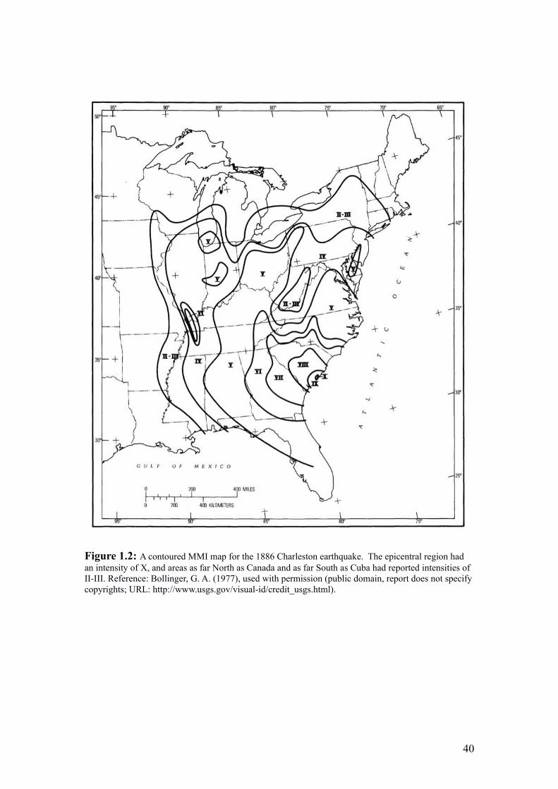
Figure 1.2: A contoured MMI map for the 1886 Charleston earthquake. The epicentral region had an intensity of X, and areas as far North as Canada and as far South as Cuba had reported intensities of II-III. Reference: Bollinger, G. A. (1977), used with permission (public domain, report does not specifycopyrights; URL: http://www.usgs.gov/visual-id/credit_usgs.html).
40

Figure 1.3: A proposed fault model for the study region. It contains an approximately 50 kilometer long NE-SW trending fault, called the Woodstock Fault (WF) with a step over fault trending to the NW-SE called the Sawmill Branch fault (SBF). Additionally there is a fault, branching off to the East called the Ashley River Fault (ARF). The circles represent located events between 1974-2004 from theSouth Eastern United States Seismic Network (SEUSSN). Reference: Dura-Gomez, I. and Talwani, P. (2009), used with permission from SSA (http://www.seismosoc.org/publications/permissions.php).
41

Figure 1.4: Detailed maps of the study region. Top: A magnetic intensity map of the study region. The colored lines represent the seismic reflection profiles from VT, USGS, and COCORP, and the wells are marked by the yellow triangles. The study region lies on a magnetic anomaly. Bottom: A more-detailed map of the study area, showing the rivers and county lines. The circles represent earthquakes epicenters (M > 2) from 1977-2004, located by the SEUSSN. Reference: Chapman, M. C. and Beale, J.N. (2010), used with permission from M.C. Chapman.
42

Figure 1.5: Processed seismic reflection profile VT3. Interpreted faults and reflectors are annotated. The bottom of the figure shows the reflection profile in map view. Reference: Chapman, M. C. and Beale, J.N. (2010), used with permission from M.C. Chapman.
43

Figure 1.6: A map of the study region showing the magnetic gradient and imaged faults. The lines composed of small dots show the locations of seismic reflection profiles (each dot is a profile station location). The location of the gradient in the magnetic field is indicated by the broad shaded line. The locations of Mesozoic-Cenozoic faults imaged on reflection profiles are indicated by the large filled circles, labeled F1 through F5. Small open circles show earthquake epicenters (M>2.0, occurring from 1977 through 2004) located by the University of South Carolina seismic network. The long-dashed linepassing approximately 4 km southeast of Summerville marks the location where southeastward dip on the bright B reflection becomes pronounced. The long-dashed line near the end of profiles C2 and SC4 marks the location where the bright B reflection shallows to the level of the J reflection, dipping to the northwest. The trough of the intervening structural basin, defined by two-way time greater than 1.1 second for the bright B reflection, is indicated by the shaded area outlined by short-dashed lines containing the southern part of reflection profile C3. The inferred Woodstock North (WN) and Woodstock South (WS) faults of Dura-Gomez and Talwani (2009) are shown as solid lines. From Chapman and Beale (2010), used with permission from M.C. Chapman.
44

Chapter 2:
Figure 2.1: The seismic network used for the monitoring experiment: The red triangles represent theeight temporary stations and the blue triangles represent the 4 permanent stations, sponsored by the ANSS (USGS) and run by the University of South Carolina. The black dots represent 134 earthquakes located by HypoEllipse (duration magnitudes ranging from -1.8-2.6).
45

Figure 2.2: A diagram illustrating the rotation of horizontal station components. . The rotation, described by Equation 2, transforms the North and East components to the Radial and Transverse components, respectively and effectively rotates the components to the direction of source propagation.
46

Figure 2.3: A flow chart outlining the processing steps carried out for each station record. The Butterworth bandpass filters were chosen, to reduce low-frequency noise and high-frequency acausal energy from the instrument FIR filter. The source azimuth was determined by initial location of the 134detectable events from Hypoellipse. The supplemental filtering was an iterative process and the filters were chosen based on comparison of the Fourier amplitude spectra of the signal and pre-signal noise.
47

Figure 2.4: A diagram comparing raw data and processed data. Top: Unprocessed 3-component station record (WSCT): North-South, East-West, and Vertical components. Bottom: Processed record (see flow chart in Figure 2.3): Radial, Transverse, Vertical components.
48

P
ConvertedPhase
SH
SV
ConvertedPhase
SV
SH
P
A
B
Figure 2.5: A: Processed 3-component station record (MTBA) with interpreted wave phases. The P wave is picked on the vertical component, the SH wave is picked on the transverse component, and the SV wave is picked on the radial component. The converted phase is also annotated, and in some cases is hard to distinguish with the S wave, particularly the SV wave. B: Another example of a processed record (MTBA) with interpreted wave phases and a large converted phase.
49

Figure 2.6: A diagram showing the convention of picking a wave phase. The polarity is determined by the peak or trough at the next half cycle following the arrival time. Polarity conventions for all wavephases are summarized in Table 2.
50

Chapter 3:
Figure 3.1: A diagram showing the 1-D velocity model. It is 3 layers over a halfspace, derived from Chapman et al. (2003). It incorporates a shallow layer with low P and S wave velocities appropriate for the coastal plain sediments, a higher velocity, upper crustal layer representative of the lower Mesozoic volcanic and sedimentary rock section, and a lower crustal velocity layer with somewhat higher wave velocities determined from refraction velocity measurements in the Piedmont province of Virginia (Bollinger et al., 1980).
51

A
Figure 3.2A: Hypocenter locations with Hypoellipse. Top: Hypocenter locations of 134 earthquakes determined using Hypoellipse, plotted as epicenters in map view. A cross-section D-D’ trending N95E is projected through the earthquakes. Bottom: The D-D’ cross section is shown, illuminating a possible trend (dashed line) of the hypocenters. Most of the events are within the upper 5km.
52

B
Figure 3.2B: Hypocenter locations with Hypoellipse: a different perspective. Top: Hypocenter locations of 134 earthquakes determined using Hypoellipse, plotted as epicenters in map view. A cross-section A-A trending N5E is projected through the earthquakes. Bottom: The A-A’ cross section is shown and are within the upper 5 km.
53

Figure 3.3A: Hypocenter locations with HypoDD. Top: Hypocenter re-locations of 87 earthquakes determined using HypoDD, plotted as epicenters in map view. A cross-section D-D’ trending N95E is projected through the earthquakes. Bottom: The D-D’ cross section is shown, illuminating a trend(dashed line) of the hypocenters, which is more clearly defined in the re-locations. A least squaresplane fitted to the hypocenters is shown as the dashed line, with strike N186E and dip 43 degrees to the West.
54
A
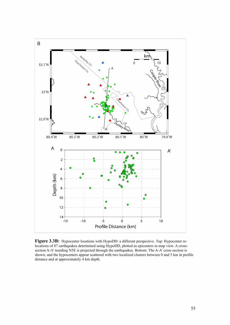
B
Figure 3.3B: Hypocenter locations with HypoDD: a different perspective. Top: Hypocenter re-locations of 87 earthquakes determined using HypoDD, plotted as epicenters in map view. A cross-section A-A’ trending N5E is projected through the earthquakes. Bottom: The A-A’ cross section is shown, and the hypocenters appear scattered with two localized clusters between 0 and 5 km in profile distance and at approximately 4 km depth.
55

Figure 3.4: A diagram summarizing definitions of strike, dip, and rake. The strike line is defined as the intersection between the planar feature and a horizontal plane in space. The strike azimuth, a, is the angle between the strike line and geographical North. The dip direction is orthogonal to the strike line, measured clockwise. The dip direction, b, is the angle between the horizontal plane and the planar feature. The slip vector is defined as the direction and magnitude of displacement of the hanging wall with respect to the footwall and the rake angle, c, is the angle between the slip vector and the strike line, positive in the counter-clockwise direction.
56

Figure 3.5: A comparison of hypocenter locations from two seismic networks. The green dots represent the hypocenters located in this study and the red represent hypocenters located from the SEUSSN (South East United States Seismic Network). The hypocenters were located by Jake Beale and Qimin Wu, using the same procedure as described in Chapter 3. The hypocenters from both networks are significantly consistent in terms of overall trend.
57

Chapter 4:
Figure 4.1: A diagram summarizing the double-couple force system. The double couple represents the force system (open arrows) responsible for shear dislocation on a plane, and is a subset of general seismic moment tensors, which characterize the motion of an earthquake source. It is assumed that moment tensors of all the events considered in this study are pure double couple.
58

Figure 4.2: A diagram of determining focal mechanisms from P-wave first motions. Focal mechanisms can be derived from first motions polarities of wave phases (left). The circles represent P-wave compressional motion, or motion towards the source (‘down’ polarity on three-component record). The triangles represent P-wave dilatational motion, or motion away from the source (‘up’ polarity on three-component record). The focal sphere can be divided into quadrants based on compressional and dilatational first motions (middle). By convention the P-wave compressional motion quadrant is shaded in black to form a beachball diagram (right).
59

Figure 4.3: A diagram showing the beachball diagrams for the 3 fundamental fault types. They include dip slip with reverse motion, dip slip with normal motion, and strike slip. There are three axes plotted on a focal mechanism/beach ball diagram: Tensional (T), Compressional/Pressure (P), and the Null (B or N). The tensional axis is located at the center of the P-wave compressional quadrant, the pressure axis is located at the center of the P-wave dilatational quadrant, and the null axis marks the intersection of the two nodal planes.
60

Figure 4.4: Comparison of focal mechanism solutions derived from different data types. Top: The focal mechanism solutions (Focmec output), derived from P-wave first motion polarity data. Bottom: The addition of a single amplitude ratio greatly improves the constraint of the focal mechanism solution by reducing the amount of possible fault-plane solutions. Reference: Chapman, M. C. and Beale, J.N. (2013), used with permission from M.C. Chapman.
61
!

Figure 4.5: Focal mechanism solutions and constraint tests for an event in the dataset. Both the bestsolution (top left) and the outputs from the constraint tests are shown. Constraint testing reveals how robust the best solution is.
62

Figure 4.6: The distribution of the 66 well-constrained focal mechanisms. The majority of the mechanisms shows reverse motion, and were therefore broken up into sub-categories by the variation in P-axis trend.
63

A
B
64

C
D
65

E
Figure 4.7, A-E: The focal mechanisms plotted with the events relocated using HypoDD. The duration magnitude and focal depth is indicated. The focal mechanisms of each category (defined in Figure 4.6) are shown in panels A through E. A: Reverse motion, E-W trend, 7 total. B: Reverse motion, NE-SW trend, 6 total. C: Reverse motion, NW-SE trend, 13 total. D: Reverse motion, N-S trend, 28 total. E: Strike-slip motion, 11 total.
66
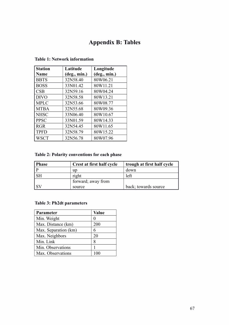
Appendix B: Tables
Table 1: Network information
Station Name
Latitude (deg., min.)
Longitude (deg., min.)
BBTS 32N58.40 80W06.21BOSS 33N01.42 80W11.21CSB 32N59.16 80W04.24DIVO 32N58.58 80W13.21MPLC 32N53.66 80W08.77MTBA 32N55.68 80W09.36NHSC 33N06.40 80W10.67PPSC 33N01.59 80W14.33RGR 32N54.45 80W11.65TPFD 32N58.79 80W15.22WSCT 32N56.78 80W07.96
Table 2: Polarity conventions for each phase
Phase Crest at first half cycle trough at first half cycleP up downSH right left
SVforward; away from source back; towards source
Table 3: Ph2dt parameters
Parameter ValueMin. Weight 0Max. Distance (km) 200Max. Separation (km) 6Max. Neighbors 20Min. Link 8Min. Observations 1Max. Observations 100
67

Table 4: HypoDD parameters
Parameter Valuemax. distance (km) 200Vp/Vs ratio 1.73IDAT (code for catalog data) 2IPHA (code for P and S phases) 3ISOLV (code for LSQR) 2NLAY (velocity model layers) 4
Table 5: Focmec parameters
Parameter ValueVp/Vs ratio at source 1.7321Max. allowed ratio deviation 0.6*Maximum no. solutions 500
Table 6: Rating system
Rating #stations #polaritiesA ≥ 7 ≥ 12B 5-7 8-12C 4 anyD 3 any
68

Table 7: Summary of Focal Mechanism Results
Event Name Type HE depths
HypoDDdepths # S # P # R rating
20110807_043200_MAN Rev_NW-SE 7.3 7.536 7 17 12 A
20110816_045000_MAN SS 2.89 3.29 7 15 11 A
20110818_025100_MAN Rev_E-W 4.195 5.627 6 14 10 B
20110820_195500_MAN Rev_N-S 5.6 - 7 17 12 A
20110821_143700_MAN Rev_NW-SE 2.43 - 8 16 9 A
20110822_061000_MAN Rev_N-S 3.45 4.04 8 13 8 A
20110822_155900_MAN SS 3.14 - 4 4 4 C
20110830_071300_MAN Rev_N-S 4.5 5.88 6 13 2 B
20110913_215900_MAN Rev_E-W 1.33 - 3 3 2 F
20110922_083300_MAN SS 3.66 3.826 4 7 8 C
20110929_000900_MAN Rev_N-S 3.88 4.5 5 9 5 B
20111008_083300_MAN Rev_N-S 6.9 7.78 5 8 5 B
20111015_070200_MAN Rev_NW-SE 11.03 12.134 7 16 11 A
20111016_081300_MAN Rev_N-S 5.62 5.016 4 6 7 C
20111021_221300_MAN Rev_N-S 4.04 4.811 4 7 6 C
20111027_035100_MAN Rev_N-S 9.45 9.4 5 8 5 B
20111031_143700_MAN Rev_E-W 3.57 4.303 5 10 6 B
20111105_164700_MAN SS 4.56 4.999 5 9 6 B
20111109_090800_MAN SS 1.96 0.635 4 7 8 C
20111111_232000_MAN Rev_NW-SE 4.35 4.826 5 15 10 B
20111112_095600_MAN Rev_N-S 4.62 4.848 8 14 14 A
20111113_022700_MAN Rev_NE-SW 3.57 3.482 4 9 8 C
20111126_123400_MAN Rev_NW-SE 4.06 4.51 7 16 11 A
20111206_213800_MAN Rev_NW-SE 1.83 1.66 4 9 6 C
20111207_094800_MAN Rev_N-S 1.5 1.341 8 16 8 A
20111211_150300_MAN Rev_N-S 4.44 5.071 5 6 5 C
20111221_213800_MAN Rev_N-S 10.88 11.43 9 21 12 A
20111226_101000_MAN Rev_N-S 3.83 3.57 6 14 10 B
20120102_002000_MAN Rev_NE-SW 3.6 4.69 8 17 12 A
20120104_075600_MAN Rev_NE-SW 3.66 4.99 9 19 12 A
20120107_174800_MAN Rev_NW-SE 4.19 4.67 6 12 6 B
20120109_215700_MAN Rev_NW-SE 4.15 4.789 9 23 12 A
20120110_063500_MAN SS 4.62 4.885 5 10 10 B
20120117_061400_MAN Rev_N-S 2.48 - 4 9 5 C
20120117_114200_MAN SS 3.08 3.34 4 10 7 C
20120117_125400_MAN Rev_NW-SE 4.12 - 3 5 4 F
20120119_104800_MAN Rev_N-S 4.35 - 4 7 3 C
20120120_195300_MAN Rev_E-W 4.31 4.528 5 10 8 B
20120121_093600_MAN Rev_NE-SW 4.06 4.583 5 9 7 B
69
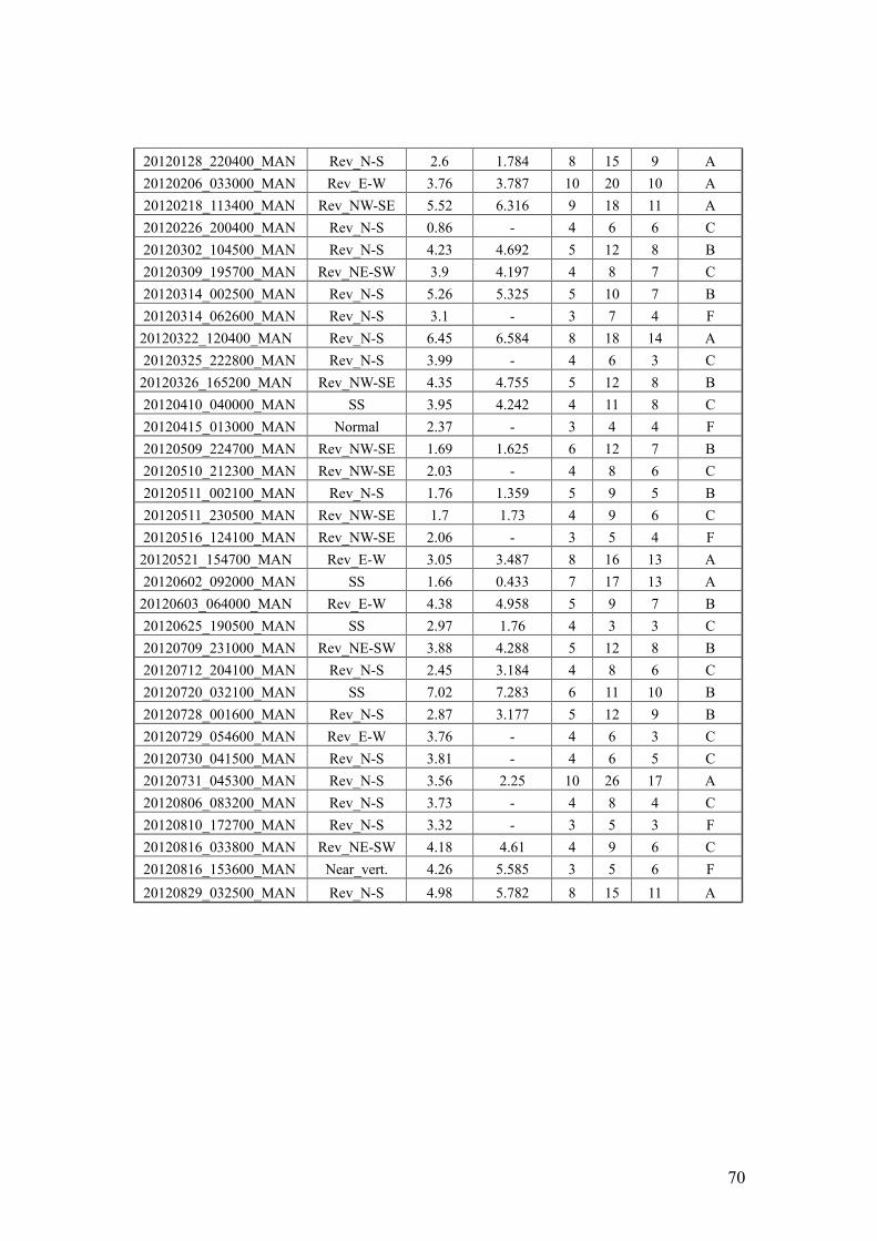
20120128_220400_MAN Rev_N-S 2.6 1.784 8 15 9 A
20120206_033000_MAN Rev_E-W 3.76 3.787 10 20 10 A
20120218_113400_MAN Rev_NW-SE 5.52 6.316 9 18 11 A
20120226_200400_MAN Rev_N-S 0.86 - 4 6 6 C
20120302_104500_MAN Rev_N-S 4.23 4.692 5 12 8 B
20120309_195700_MAN Rev_NE-SW 3.9 4.197 4 8 7 C
20120314_002500_MAN Rev_N-S 5.26 5.325 5 10 7 B
20120314_062600_MAN Rev_N-S 3.1 - 3 7 4 F
20120322_120400_MAN Rev_N-S 6.45 6.584 8 18 14 A
20120325_222800_MAN Rev_N-S 3.99 - 4 6 3 C
20120326_165200_MAN Rev_NW-SE 4.35 4.755 5 12 8 B
20120410_040000_MAN SS 3.95 4.242 4 11 8 C
20120415_013000_MAN Normal 2.37 - 3 4 4 F
20120509_224700_MAN Rev_NW-SE 1.69 1.625 6 12 7 B
20120510_212300_MAN Rev_NW-SE 2.03 - 4 8 6 C
20120511_002100_MAN Rev_N-S 1.76 1.359 5 9 5 B
20120511_230500_MAN Rev_NW-SE 1.7 1.73 4 9 6 C
20120516_124100_MAN Rev_NW-SE 2.06 - 3 5 4 F
20120521_154700_MAN Rev_E-W 3.05 3.487 8 16 13 A
20120602_092000_MAN SS 1.66 0.433 7 17 13 A
20120603_064000_MAN Rev_E-W 4.38 4.958 5 9 7 B
20120625_190500_MAN SS 2.97 1.76 4 3 3 C
20120709_231000_MAN Rev_NE-SW 3.88 4.288 5 12 8 B
20120712_204100_MAN Rev_N-S 2.45 3.184 4 8 6 C
20120720_032100_MAN SS 7.02 7.283 6 11 10 B
20120728_001600_MAN Rev_N-S 2.87 3.177 5 12 9 B
20120729_054600_MAN Rev_E-W 3.76 - 4 6 3 C
20120730_041500_MAN Rev_N-S 3.81 - 4 6 5 C
20120731_045300_MAN Rev_N-S 3.56 2.25 10 26 17 A
20120806_083200_MAN Rev_N-S 3.73 - 4 8 4 C
20120810_172700_MAN Rev_N-S 3.32 - 3 5 3 F
20120816_033800_MAN Rev_NE-SW 4.18 4.61 4 9 6 C
20120816_153600_MAN Near_vert. 4.26 5.585 3 5 6 F
20120829_032500_MAN Rev_N-S 4.98 5.782 8 15 11 A
70