Hyperspherical Approach to Quantal Three-body Theory

by

Jia Wang

B.A., Tsinghua University, 2004

M.Phil., Chinese University of Hong Kong, 2006

A thesis submitted to the

Faculty of the Graduate School of the

University of Colorado in partial fulfillment

of the requirements for the degree of

Doctor of Philosophy

Department of Physics

2012

This thesis entitled:Hyperspherical Approach to Quantal Three-body Theory

written by Jia Wanghas been approved for the Department of Physics

Chris H. Greene

Prof. John Bohn

Prof. Eric Cornell

Date

The final copy of this thesis has been examined by the signatories, and we find that both thecontent and the form meet acceptable presentation standards of scholarly work in the above

mentioned discipline.

iii

Wang, Jia (Ph.D., Physics)

Hyperspherical Approach to Quantal Three-body Theory

Thesis directed by Prof. Chris H. Greene

Hyperspherical coordinates provide a systematic way of describing three-body systems. Solv-

ing three-body Schrodinger equations in an adiabatic hyperspherical representation is the focus of

this thesis. An essentially exact solution can be found numerically by including nonadiabatic cou-

plings using either a slow variable discretization or a traditional adiabatic method. Two different

types of three-body systems are investigated: (1) rovibrational states of the triatomic hydrogen ion

H+3 and (2) ultracold collisions of three identical bosons.

Dedication

To my love.

Acknowledgements

First and foremost, I’d like to thank my advisor Chris H. Greene, for his patience, motivation,

enthusiasm, and immense knowledge. Working with Chris is a great experience, not only because

of his unparalleled knowledge of atomic and molecular physics, but also because he has always been

supportive of my career. He is also a nice and easygoing person, and will always be a role model

in my life.

Besides Chris, working with other people in Greene’s group is also a very nice experience.

Jose D’Incao has always been a great teacher and big brother for me. Learning and discussing

physics with him is always pleasant. I also owe many thanks to Yujun Wang. He has been very

helpful in various projects during the last year. I also want to thank all the other group members:

Michal Tarana, Chen Zhang, John Papaioannou, Nathan Morrison, Stephen Ragole, Victor Colussi,

Minghui Xu and Javier von Stecher for all the discussions about physics during our fun group

meetings and vast spare time. Previous group members Daniel Haxton, Zach Walters, Nirav Mehta

and Seth Rittenhouse have also helped me a lot during my PhD years.

I would also like to thank the people outside the Greene group that I have gotten the pleasure

of working with directly. Viatcheslav Kokoouline has given me tremendous help in the H+3 project.

I would like to thank Richard Saykally and his group for sharing their beautiful experimental results

with us. From the collaboration with Brett Esry, I learned how to think critically and how to be

scientifically rigorous. Having the opportunity to collaborate with Eric Cornell is also a valuable

experience. I am always amazed by his great intuition of telling the underlying physics out of

complex phenomena.

vi

I would also like to thank my Master advisor Chi Kwong Law and Ming Chung Chu in the

Chinese University of Hong Kong, for bringing me into the beautiful world of atomic and molecular

physics and giving me a strict training in scientific research.

I also owe many thanks to Peter Ruprecht and James McKown for all their technical support,

and to Pam Leland for her administrative support.

I would like to thank all of my friends for supporting me and encouraging me with their best

wishes. A special thanks goes to Yiqing Xie for her endless support during the last five years. Last

but not least, I would like to thank my family for their unconditional support throughout my life.

I have received funding support from the National Science Foundation, the Department of

Energy, and the Air Force Office of Scientific Research for this work.

vii

Contents

Chapter

1 Introduction 1

2 Adiabatic Hyperspherical Approach 8

2.1 Hyperspherical coordinate . . . . . . . . . . . . . . . . . . . . . . . . . . . . . . . . . 8

2.2 Adiabatic hyperspherical representation . . . . . . . . . . . . . . . . . . . . . . . . . 10

2.3 Coupling matrices . . . . . . . . . . . . . . . . . . . . . . . . . . . . . . . . . . . . . 13

2.4 Slow variable discretization (SVD) method . . . . . . . . . . . . . . . . . . . . . . . 17

2.4.1 Bound-state calculations . . . . . . . . . . . . . . . . . . . . . . . . . . . . . . 18

2.4.2 Scattering calculations . . . . . . . . . . . . . . . . . . . . . . . . . . . . . . . 18

3 Rovibrational states of H3+ and quantum-defect analysis of H3 Rydberg states 22

3.1 Introduction . . . . . . . . . . . . . . . . . . . . . . . . . . . . . . . . . . . . . . . . . 22

3.2 Rovibrational states of H+3 . . . . . . . . . . . . . . . . . . . . . . . . . . . . . . . . . 25

3.2.1 Adiabatic representation . . . . . . . . . . . . . . . . . . . . . . . . . . . . . . 25

3.2.2 Accuracy of the rovibrational energies of H+3 . . . . . . . . . . . . . . . . . . 28

3.2.3 Rovibrational-frame transformation . . . . . . . . . . . . . . . . . . . . . . . 28

3.3 p-wave energy levels of H3 . . . . . . . . . . . . . . . . . . . . . . . . . . . . . . . . . 31

3.3.1 Body-frame quantum defects for p-waves . . . . . . . . . . . . . . . . . . . . 31

3.3.2 3p1 energy levels of H3 . . . . . . . . . . . . . . . . . . . . . . . . . . . . . . . 33

3.4 Higher angular-momentum states . . . . . . . . . . . . . . . . . . . . . . . . . . . . . 33

viii

3.5 Recombination-pumped triatomic hydrogen infrared lasers . . . . . . . . . . . . . . . 37

3.6 Summary . . . . . . . . . . . . . . . . . . . . . . . . . . . . . . . . . . . . . . . . . . 43

4 Numerical study of three-body recombination 44

4.1 Introduction . . . . . . . . . . . . . . . . . . . . . . . . . . . . . . . . . . . . . . . . . 44

4.2 Adiabatic hyperspherical representation . . . . . . . . . . . . . . . . . . . . . . . . . 47

4.3 Three-body recombination rates . . . . . . . . . . . . . . . . . . . . . . . . . . . . . . 48

4.4 Dominant recombination pathways . . . . . . . . . . . . . . . . . . . . . . . . . . . . 57

4.5 Summary . . . . . . . . . . . . . . . . . . . . . . . . . . . . . . . . . . . . . . . . . . 61

5 Origin of the Three-body Parameter Universality in Efimov Physics 62

5.1 Introduction . . . . . . . . . . . . . . . . . . . . . . . . . . . . . . . . . . . . . . . . . 63

5.2 Van der Waals interaction and classical suppression . . . . . . . . . . . . . . . . . . . 64

5.2.1 Van der Waals interaction . . . . . . . . . . . . . . . . . . . . . . . . . . . . . 65

5.2.2 Classical (WKB) Suppression . . . . . . . . . . . . . . . . . . . . . . . . . . . 66

5.3 Three-body adiabatic hyperspherical representation . . . . . . . . . . . . . . . . . . . 73

5.4 Three-body parameters . . . . . . . . . . . . . . . . . . . . . . . . . . . . . . . . . . 76

5.4.1 Universality of the three-body parameter . . . . . . . . . . . . . . . . . . . . 80

5.4.2 Single channel approximation . . . . . . . . . . . . . . . . . . . . . . . . . . . 85

5.5 Summary . . . . . . . . . . . . . . . . . . . . . . . . . . . . . . . . . . . . . . . . . . 89

6 Efimov physics on the positive side 92

6.1 Stuckelberg minima . . . . . . . . . . . . . . . . . . . . . . . . . . . . . . . . . . . . 93

6.2 Three-body recombination resonances associated with d-wave interactions . . . . . . 93

6.3 Three-body state associated with the d-wave dimmer . . . . . . . . . . . . . . . . . . 101

6.4 Summary . . . . . . . . . . . . . . . . . . . . . . . . . . . . . . . . . . . . . . . . . . 103

ix

Bibliography 106

Appendix

A Symmetry of R-matrix 112

B R-matrix propagation method with the traditional adiabatic method. 114

C Permutation symmetry of the basis functions 116

D Body-frame quantum defect matrix elements 119

E Effective adiabatic potentials 123

x

Tables

Table

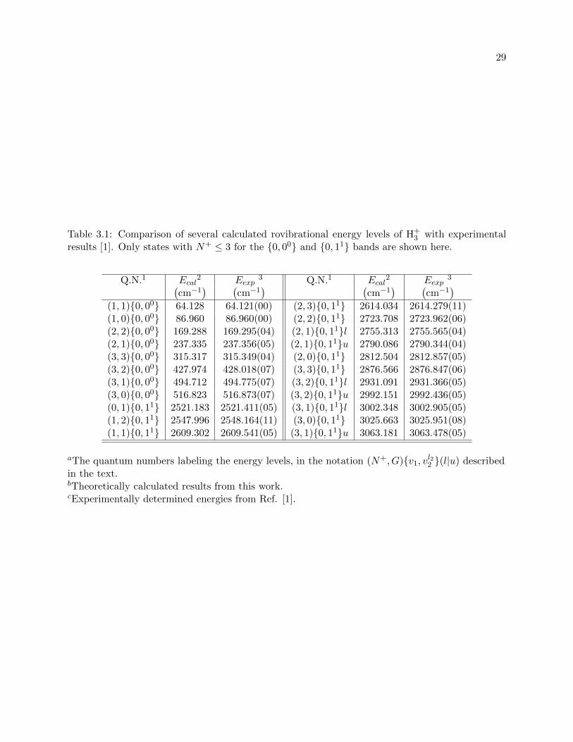
3.1 Comparison of several calculated rovibrational energy levels of H+3 with experimental

results [1]. Only states with N+ ≤ 3 for the 0, 00 and 0, 11 bands are shown here. 29

3.2 A comparison between several of our calculated 3p1 H3 energy levels with empirically

fitted experimental energy levels [2, 3, 4, 5]. . . . . . . . . . . . . . . . . . . . . . . . 34

3.3 Comparison between several of our calculated 3d energy levels of H3 with experimentally-

determined energy levels[2, 3, 4, 5]. . . . . . . . . . . . . . . . . . . . . . . . . . . . . 36

3.4 Possible assignment of laser lines observed in this work. We calculate the theory

lines by using models described in this chapter. The experiment lines are chosen

from the H2O – He laser lines which are also observed in H2O – He or H2O – Ne

experiments. . . . . . . . . . . . . . . . . . . . . . . . . . . . . . . . . . . . . . . . . 41

C.1 Permutation symmetry for basis functions in the different degrees of freedom. . . . . 117

xi

Figures

Figure

3.1 (Color online) Lowest 60 adiabatic potential curves U (R) of H+3 with total angular

momentum N+ = 1, odd parity and gI = 1. The dashed horizontal line shows the

lowest rovibrational ground state of this system. . . . . . . . . . . . . . . . . . . . . 27

3.2 Comparison of experimental results with calculated nd→ n′p transitions of H3. The

experimental laser strength is in arbitrary units with linear scale, while the present

theoretical B-coefficients are in the units of 1022 (m/Js2) on a logarithmic scale. The

calculated line positions have a precision of about 13 cm−1 . . . . . . . . . . . . . . 40

4.1 (Color online) Adiabatic potential curves U (R) at short distances R. Red solid lines

represent the three-body continuum channels, i.e., the initial channels for recombi-

nation processes, and black dashed lines represent the final recombination channels. 49

4.2 (Color online) Same as Fig. 4.1, but for the adiabatic potential curves U (R) at large

distances R. This figure contrasts with Fig. 4.1 in the characteristically smooth

behavior at large distances. . . . . . . . . . . . . . . . . . . . . . . . . . . . . . . . . 50

xii

4.3 (Color online) Partial recombination rate K(f←i)3 as a function of the collision energy

E for the positive-scattering length case. The solid, dashed, dot, dash-dot and short

dashed lines indicate partial recombination rates to different recombination channels:

f = 1, 2, 3, 4, 5, respectively. The thick black lines, thinner red lines and thinnest

blue lines indicate recombination rates from different incident channels: i = 1, 2, 3.

The three green dash-dot-dot lines are proportional to E0, E1 and E4 as indicated

in the figure. . . . . . . . . . . . . . . . . . . . . . . . . . . . . . . . . . . . . . . . . 53

4.4 (Color online) Same as Fig. 4.3 but for the negative scattering length case. . . . . . 54

4.5 (Color online) Branching ratio of the calculated recombination rates r(f←i)3 as func-

tions of the collision energy E for the positive-scattering length case. The line-styles

solid, dashed, dot, dash-dot and short-dashed indicate recombination rate to different

recombination channels: f = 1, 2, 3, 4, 5, respectively. The thick black lines, thinner

red lines and thinnest blue lines indicate recombination rates from three different

incident channels: i = 1, 2, 3. The inset shows the branching ratio between the deep

bound states only and it excludes the shallowest bound state (see the text for further

details). . . . . . . . . . . . . . . . . . . . . . . . . . . . . . . . . . . . . . . . . . . . 55

4.6 (Color online) Same as Fig. 4.5 but for the negative scattering length case. . . . . . 56

5.1 Lennard-Jones potential with the 2nd, 3rd and 4th s-wave bound state exactly at

the threshold (denoted by λ = λ∗2, λ∗3, λ∗4). The insert shows the corresponding zero-

energy wave function. . . . . . . . . . . . . . . . . . . . . . . . . . . . . . . . . . . . 68

5.2 Effective ranges at the pole as a function of the potential depths D∗n for vsch. . . . . 70

xiii

5.3 The red solid curve represents the scattering length, a/r0, while the green dashed

curve represents the parameter ξinp (k → 0). Both quantities are plotted as functions

of the depth D of the two-body interaction model vsch [Eq. (5.2)], whose values

for which |a| = ∞ are indicated in the figure as D∗n, where n is the number of

s-wave states. The black circles, open circles, and open squares are the values of

ξinp at |a| → ∞, a = 5r0, and a = −5r0, respectively. Their trends documents the

suppression of the ξinp as the number of bound states increases. The results for ξin

p also

show higher efficiency of the suppression inside the well for |a|/r0 1. The black

dash-dotted curve shows the suppression factor 1/kL(r0), confirming the classical

origin of the suppression mechanism. . . . . . . . . . . . . . . . . . . . . . . . . . . 72

5.4 (a) Full energy landscape for the three-body potentials at a = ∞ for our vaλ model

potential. (b) Effective diabatic potentials Wν relevant for Efimov physics for vaλ with

an increasingly large number of bound states (λ∗n is the value of λ that produces a =

∞ and n s-wave bound states). The Wν converge to a universal potential displaying

the repulsive barrier at R ≈ 2rvdW that prevents particles access to short distances.

(c)–(e) demonstrate the suppression of the wave function inside the potential well

through the channel functions Φν(R; θ, ϕ) for R fixed near the minima of the Efimov

potentials in (b). (c) shows the mapping of the geometrical configurations onto the

hyperangles θ and ϕ. (d) and (e) show the channel functions, where the “distance”

from the origin determines |Φν |1/2, for two distinct cases: in (d) when there is a

substantial probability of finding two particles inside the potential well (defined by

the region containing the gray disks) and in (e) with a reduced probability — see

also our discussion in Fig. 5.5. In (d) and (e), we used the potentials vsch and vaλ,

respectively, both with n = 3. . . . . . . . . . . . . . . . . . . . . . . . . . . . . . . . 74

xiv

5.5 Density plot of the three-body probability density |Φν(R; θ, ϕ)|2 sin 2θ that deter-

mines the three particle configuration [see Fig. 5.4 (c)] in the θ-ϕ hyperangular plane

for a fixed R (sin 2θ is the volume element). (a)–(d) show the results for an R near

the minima of the Efimov potentials in Fig. 5.4 (b) for the first four scattering length

poles of the vaλ model, as indicated. (a) shows that there is a negligible probability

of finding the particles at distances smaller than rvdW (outer dashed circle) and, of

course, inside the 1/r12 repulsive barrier (inner solid circle). For higher poles, i.e., as

the strength of the hard-core part of vaλ potential decreases, the potential becomes

deeper and penetration into the region r < rvdW is now classically allowed. Never-

theless, (b)–(e) show that inside-the-well suppression still efficiently suppresses the

probability of finding particle pairs at distances r < rvdW, found to be in the range

2–4%. . . . . . . . . . . . . . . . . . . . . . . . . . . . . . . . . . . . . . . . . . . . . 75

5.6 The Efimov potential obtained from the different two-body potential models used

here. The reasonably good agreement between the results obtained using models

supporting many bound states (vsch, vaλ and vbλ) and vhsvdW [obtained by replacing the

deep potential well with a hard wall but having only one (zero-energy) bound state]

supports our conclusion that the inside-the-well suppression of the wave function

is the main physical mechanism behind the universality of the three-body effective

potentials. The differences between these potentials are seen to cause differences of

a few percent in the three-body parameter. . . . . . . . . . . . . . . . . . . . . . . . 77

5.7 Fitting the Efimov resonance using a fano lineshape [Eq. (5.16)] for a system using

the two-body model potential vaλ with λ = λ∗2. The blue circles, red triangles,

and black squares are the numerically calculated |1 − Sii|2 for the three deeper

atom-dimer channels (a g-wave dimer, a d-wave dimer, and a deeper s-wave dimer,

correspondingly.) The curves are fitting results from using Eq. (5.16). . . . . . . . . 79

5.8 Efimov scenario calculated for vbλ with λ = λ∗2. Both the ground and first excited

Efimov spectra as a function of sign(a)(a/rvdW)1/4are shown. . . . . . . . . . . . . . 81

xv

5.9 The Efimov resonance corresponding to the Efimov ground state. The black squares

are numerically calculated results, and the solid curve is the fitting result from using

Eq. (5.17). . . . . . . . . . . . . . . . . . . . . . . . . . . . . . . . . . . . . . . . . . 82

5.10 Values for the three-body parameter (a) κ∗ and (b) a−3b as functions of the number

n of two-body s-wave bound states for each of the potential model studied here. (c)

Experimental values for a−3b for 133Cs [6] (red: ×, +, , and ∗), 39K [7] (magenta:

M), 7Li [8] (blue: •) and [9, 10] (green: and ), 6Li [11, 12] (cyan: N and O) and

[13, 14] (brown: H and ♦), and 85Rb [15] (black: ). The gray region specifies a

band where there is a ±15% deviation from the vhsvdW results. The inset of (a) shows

the suppression parameter ξinp [Eq. (5.11)] which can be roughly understood as the

degree of sensitivity to nonuniversal corrections. Since ξinp is always finite — even in

the large n limit — nonuniversal effects associated with the details of the short-range

interactions can still play an important role. One example is the large deviation in

κ∗ found for the vsch (n = 6) model, caused by a weakly bound g-wave state. For

n > 10 we expect κ∗ and a−3b to lie within the range of 15% established for n ≤ 10. . 84

5.11 (a) This figure compares the energies (as characterized by the three-body parameter

κ∗) obtained from a single channel approximation with our full calculations. The

three-body parameter κ∗ is shown for the vaλ model in the single channel approxi-

mation (open triangles) as well as for our full numerical results (open circles). The

single channel approximation can be improved by imposing a simple change in the

adiabatic potentials near the barrier, as is shown in (b). There we smoothly connect

the potential for vaλ (red solid line) to the barrier obtained for vhsvdW (black solid

line), resulting in the potential labeled by vaλ (green solid line). This new potential

is actually more repulsive and has energies [filled circles in (a)] that are much closer

to our full numerical calculations. . . . . . . . . . . . . . . . . . . . . . . . . . . . . . 86

xvi

5.12 This figure shows the three-body potentials obtained using the vaλ(λ = λ∗10) model

supporting a total of 100 bound states. Roughly speaking, the potential of Eq. (5.18) [16]

(black solid line) can be seen as a diabatic potential since it passes near one of the

series of avoided crossings. . . . . . . . . . . . . . . . . . . . . . . . . . . . . . . . . . 88

5.13 Comparison between the effective potential obtained from Ref. [16] and the potential

from Eq. (5.20). . . . . . . . . . . . . . . . . . . . . . . . . . . . . . . . . . . . . . . 90

6.1 The three-body recombination rate K3 as a function of scattering length a. The

black curve with square symbols shows the results from a Lennard-Jones potential

with two s-wave bound states; the red curve with circles illustrates the results for

three s-wave bound states. A Stuckelberg minimum appears at about a = 28.09rvdW

for both cases; the minimum is indicated by a vertical dashed line. Two enhancement

features are also shown for both cases near the small scattering length of a ≈ 0.956

rvdW. The green dashed line is proportional to a4, the overall scaling of K3. . . . . . 94

6.2 The total and partial three-body recombination rate K3 as a function of scattering

length a. The black curve with square symbols shows the total recombination rate,

and the red curve with circle symbols shows the partial recombination rate for the

shallowest s-wave dimer channel. The other curves shows the partial recombination

rate for deeper atom-dimer channels. The Stuckelberg minimum only shows up in

the shallowest s-wave dimmer channel, but not the deeper atom-dimer channels. . . 95

6.3 The two-body s-wave scattering length a∗l when a d-wave (l = 2) dimer (black curve

with square symbols) or an i-wave (l = 6) dimer becomes bound (red curve with

circle symbols), shown as functions of the number of two-body s-wave bound states. 97

xvii

6.4 Adiabatic potential curves for a ≈ 0.977. The 2+1 channels, which corresponding to

a dimer plus an atom at very large distance, are labeled by a combination of a letter

and a number. The letter denotes the angular momentum quantum number of the

dimer, and the number labels the channels for the same dimer angular momentum

from low-to-high dimer energies. . . . . . . . . . . . . . . . . . . . . . . . . . . . . . 98

6.5 Total and partial three-body recombination rate as a function of two-body scattering

length a, shown on a linear scale, near a d-wave dimer that is just becoming bound.

The inset shows the same graph with a logarithmic scale for the y axis. The solid

vertical line shows the s-wave scattering length when the d-wave dimer becomes

bound. The two dashed vertical lines show the two peaks of recombination rate

enhancement, denoted A and B respectively. . . . . . . . . . . . . . . . . . . . . . . . 100

6.6 (I) Wνν(R) as a function of hyperradius R at the K3 resonance peak A. (II) W (R)νν

as a function of hyperradius R around the K3 enhancement peak B. The inset shows

the three points where the potential curves correspond to. . . . . . . . . . . . . . . . 102

6.7 Energy of the three-body bound state associated with a d-wave dimer as a function

of scattering length a. . . . . . . . . . . . . . . . . . . . . . . . . . . . . . . . . . . . 104

6.8 The enhancements for the total three-body recombination rate at about a = 0.995rvdW

for Lennard-Jones potential with 2 and 3 s-wave bound states. . . . . . . . . . . . . 105

xviii

E.1 Comparison of Uν(R) (green dashed curves) and Wν(R) (red solid curves) demon-

strating the importance of nonadiabatic effects introduced by Qνν(R). (a) and (b)

show the results for the potential models vaλ(λ = λ∗2) and vaλ(λ = λ∗10) [Eq. (5.3)],

respectively, and in (c) we show the results obtained for vsch(D = D∗6) [Eq. (5.2)]. (a)

and (b) also show the effect of the diabatization scheme used in order to prepare some

of our figures in the main text (dash-dotted curves). The goal of the diabatization is

to eliminate the sharp features resulting from Qνν(R) which should not contribute

substantially to the three-body observables. The case shown in (c), however, does

not allow us to easily trace the diabatic version of the potentials Wν . In this case,

however, the “less” sharp features have a larger contribution due to the crossing with

a three-body channel describing a collision between a g-wave molecular state and a

free atom, giving rise to the anomalous n = 6 point for the vsch model in Fig. 4 of

the main text. Although such cases are relatively infrequent in our calculations (and

occur mostly for the vsch model), they do illustrate nonuniversal effects that can

affect the three-body parameter. Nevertheless, the three-body observables obtained

for cases like the one shown in (c) are still within the 15% range we claimed for the

universality of the three-body parameter. . . . . . . . . . . . . . . . . . . . . . . . . 124

Chapter 1

Introduction

The studies of three-body systems have a long and interesting history. In 1687, Sir Isaac

Newton started studying the gravitational problem of three-body systems and presented some

results in his famous “Principia” [17]. One of the most important applications at that time was

for studies of the motion of the Moon under the gravitational influence of the Earth and the Sun

as lunar theory [18]. During work to improve the accuracy of the lunar theory Henri Poincare’s

research in the late nineteenth century led to the beginning of chaos theory. Poincare extended the

problem from the Earth-Moon-Sun system to general three-body systems with mutual gravitational

interactions, as the “three-body problem”. Because of this study, he won the prize competition

in honor of the 60th birthday of King Oscar II of Sweden in 1889. Poincare discovered that such

a system, under certain conditions, can exhibit chaotic behavior that is highly sensitive to initial

conditions but impossible to predict in the long term. Chaotic behavior is described by the nonlinear

differential equation governing the dynamics of a classical three-body system. However, such chaotic

behavior would not exist in a classical sense for a quantal three-body system whose dynamic is

governed by the linear Schrodinger equation. Nevertheless, the study of how chaotic classical

dynamics can be described in terms of quantum theory became an interesting question, and leads

to the beginning of quantum chaos theory in the twentieth century [19].

The studies of quantum chaos raise an interesting question: can quantum mechanics describe

the exotic behaviors of three-body systems? Quantum mechanics has been proved to be very

successful in describing two-body systems. One example is that for two particles interacting with

2

each other via a short-range interaction at ultracold temperatures, one single parameter, s-wave

scattering length a, is sufficient to characterize the system. This simple description is verified by

using a to determine the properties of a sufficiently dilute homogeneous Bose-Einstein condensation

(BEC) [20] and compare them with experimental observations [21, 22, 23]. However, when the

experimentally achieved densities become greater and greater, physicists have realized that the

description of the system only in terms of two-body interactions is no longer sufficient. Quantum

calculations of a three-body system are then a natural extension of two-body analogies and serve

as a key meeting point for theoretical and experimental efforts to understand few-body physics. In

this thesis, we use the hyperspherical coordinate approach to study three-body systems.

Hyperspherical coordinates have been applied successfully in several areas of theoretical

physics ranging from nuclear physics [24, 25, 26] to atomic structure [27, 28, 29, 30] and fun-

damental few-body scattering [31, 32]. In a three-body system, there are nine degrees of freedom

in total. After separating out the center-of-mass motion, the remaining six degrees of motion can

be described by three Euler angles (α, β, γ) and three internal coordinates: the hyperradius R

and two hyperangles, θ and φ. In particular, the hyperradius R represents the overall size of the

system. Some of the deepest insights into the nature of the three-body problem have emerged

from Macek’s adiabatic hyperspherical methodology [27]. In this method, the Hamiltonian of the

system is initially diagonalized at fixed values of the hyperradius R, and the eigenvalues yield a

set of 1D-coupled adiabatic potential curves that represent the energy of the system as a function

of R. The resulting eigenfunctions can be used to develop the coupling matrices between these

potential curves. These potentials and couplings not only can be used for almost exact numeri-

cal calculation, but also help to build an intuitive understanding of the system. The potentials

can describe available reaction pathways by indicating the threshold laws and scaling laws for the

corresponding reactions. They also give information about the bound/quasi-bound states of the

system and the excitation and decay mechanisms of these states. Furthermore, the coupling matrix

elements allow accurate calculations of the full three-body Schrodinger equation for bound-state

problems and two-body inelastic and rearrangement collisions (A + BC → AB + C), three-body

3

collisions (A+B + C), and photon-assisted collision processes.

The application of the hyperspherical-coordinates approach to quantal three-body problems

dates back at least as far as the pioneering work of Llwellen Hilleth Thomas in 1935 [33]. He realized

a striking quantum effect in a three-body system: when the ratio between the potential range (r0)

and s-wave scattering length (a) becomes arbitrarily small, r0/a → 0, the ground state energy of

the system can “collapse” to E → −∞. This effect is known as the Thomas collapse. In this

case, all three particles collapse into an infinitely small size with an infinitely large binding energy.

This phenomenon can be understood in the hyperspherical picture. The effective hyperspherical

potential of such a system has the form of −(s2

0 + 1/4)/(2µ3bR

2)

for r0 R a, where µ3b is

the three-body reduced mass. The parameter s0 is universal, i.e., it does not depend on the form of

interaction as long as r0/a→ 0. For three identical bosons, s0 = 1.00624. It is well known that such

potentials can support an infinite number of bound states and that all the nearby eigen energies are

related with a geometric scaling factor En+1/En = exp (−2π/s0). Clearly, this geometric scaling

factor is also universal [exp (π/s0) ≈ 22.7 for three identical bosons]. This universal scaling factor

implies that when n approaches −∞, infinitely tightly bound states (called Thomas’s collapse

states) exist. In real physical systems, however, the range of interparticle interactions r0 can never

be zero. Presumably, this fact prevents a Thomas collapse from being observed. On the other hand,

there is no similar obstacle to observing a closely related quantum effect, namely the Efimov effect,

as n approaches +∞. In 1970, Efimov predicted that when a two-body bound state is exactly at

the threshold, i.e., a → ∞, there is an infinite number of bound states just below the three-body

break-up threshold [26]. These states, called Efimov states, also obey En+1/En = exp (−2π/s0)

as a result of the −(s2

0 + 1/4)/(2µ3bR

2)

potential for R r0, which is usually called the Efimov

potential.

The fact that Efimov effect is universal implies that it can exist in any systems of three

identical bosons interacting with each other via short-range interactions. Ultracold atomic gases

are perfect systems for studying Efimov effects experimentally, because of the extraordinary degree

of control for such systems. Using techniques such as laser cooling and subsequent evaporative

4

cooling of atomic gases, the experimentalists can now reach the nano Kelvin range with high

densities (between about 1012 and 1015 cm−3), and finally attain BEC [21, 22, 23]. In addition,

applications of Feshbach resonances allow physicists to control the scattering length a between

ultracold atoms and study the properties of condensates. In particular, when three free particles

collide at ultracold temperatures, they can form a two-body bound state and a free particle, which

is called a three-body recombination (A+A+A→ A2 +A). This recombination process normally

releases a large amount of kinetic energy, producing atomic losses that often limit the lifetimes

of Bose-Einstein condensates [34]. Theoretical studies indicate that there is an a4 scaling of the

field-free recombination rate of three identical bosons that leads to a catastrophic loss of atoms

even if a is not quite large. Three-body recombination is a process that is also closely related with

the Efimov effects. When a is much larger than the range of two-body interaction r0 but still finite,

Efimov states can cause interference and resonant effects in three-body recombination processes

when they cross thresholds. The hyperspherical approach gives a comprehensive description of

three-body recombination and a fundamental understanding of how Efimov states affect three-

body recombination [35, 36].

Hyperspherical coordinate has also been applied to study triatomic molecules. As the simplest

triatomic molecule, H+3 is an interesting system that attracts theorists to high-accuracy quantum

calculations. H+3 also plays an important role in astrophysics since it acts as a proton donor in

chemical reactions occurring in interstellar clouds [37, 38]. Furthermore, this ion also helps to

characterize Jupiter’s atmosphere from afar [39, 40]. H+3 is the dominant positively charged ion

in molecular hydrogen plasmas and was first identified in 1911 by J. J. Thomson with an early

form of mass spectrometry [41]. Without a stable electronic excited state and a permanent dipole

moment, H+3 cannot be observed by electronic spectroscopy or rotational spectroscopy. Therefore,

an infrared rotation-vibration spectrum is the only mean to observe this ion. The first observation

was carried out by T. Oka in 1980 [42]. By 2012, more than 600 low-lying rovibrational states

of H+3 had been identified. The good agreement between the experimental spectrum and a first-

principles calculation provided a benchmark for calculations on other polyatomic molecules such

5

as water. Application of the hyperspherical approach to study H+3 leads to a better understanding

of a quantum phenomenon that once was considered mysterious and esoteric. This phenomenon is

the dissociative recombination (DR) of H+3

e− + H+3 →

H2 + H

H + H + H,

(1.1)

which is one of the key process to understand chemical reactions in diffuse interstellar clouds

[43]. However, there once was a three-orders-of-magnitude discrepancy between the theoretical and

experimental DR rate of H+3 . This discrepancy was finally dissolved by Kokoouline and Greene

in 2003 using the hyperspherical approach [31]. The use of hyperspherical coordinates has both

a practical computational advantage and a qualitative conceptual advantage in this problem. For

instance, the theory of DR is much better understood for a diatomic target than for a polyatomic

target, so the use of an adiabatic hyperspherical representation of the nuclear positions ultimately

maps polyatomic DR theory back in terms of the more familiar diatomic DR theory. In addition,

applying the hyperspherical approach to describe the coupling between an incident electron and the

vibrational or dissociative degrees of freedom of H+3 permits a natural inclusion of the Jahn-Teller

coupling and dissolves this discrepancy [31].

In this dissertation, we apply the adiabatic hyperspherical approach to investigate two differ-

ent types of three-body systems: (1) rovibrational states of the triatomic hydrogen ion, H+3 and (2)

ultracold collisions of three identical bosons. Both systems provided interesting questions and rich

physics to explore. The remainder of this thesis is organized as follows. Chapter two discusses the

details of our numercial approach, the adiabatic hyperspherical representation. The hyperspherical

coordinates used in this thesis are first introduced. Then the numerical methods for both bound

states and scattering-state calculations are elaborated.

In chapter three, we calculate the rovibrational states of H+3 with the tools described in the

last chapter. We model H+3 as three protons interacting with each other on a potential surface. Our

calculation gives rovibrational energies that are in good agreement with experimental results. In

addition, using accurate rovibrational-state wave functions, we apply multichannel quantum defect

6

theory to studying the Rydberg energy levels of H3, which consists of a Rydberg electron and an

H+3 ion core. The interaction between the Rydberg electron and the ion core is described via body-

frame quantum defects. We perform the rovibrational-frame transformation with rovibrational wave

functions of H+3 to obtain laboratory-frame quantum defects that are used to calculate both the

energy levels and the mid-infrared spectrum of the H3 Rydberg states. The mid-infrared spectrum

corresponds reasonably well with the laser lines recently observed in hydrogen/rare gas discharges

[44, 45], indicating that H3 is a likely candidate for the carrier of these lasing transitions. A lasing

mechanism for the population inversion is also proposed.

In chapter four, we study another type of three-body system: three-body recombination at

ultracold temperature. In this chapter, we study three-body recombination processes numerically

for a system of three identical bosons with a much more realistic model than used in previous

studies. Our two-body model potentials support many bound states, which is a major leap in

complexity. Our study indicates that recombination into deeply bound states can be described

by the dominance of one decay pathway, resulting from the strong coupling between different

recombination channels. Moreover, the usual Wigner threshold law must be modified for excited-

incident recombination channels. Three-body recombination has also been recognized as one of the

most important scattering observables in which features related to the universal Efimov physics

can be manifested, which will be studied it in the next chapter.

In chapter five, problems related to Efimov physics are studied. Efimov physics predicts that

there are an infinite number of three-body bound states for a three-identical-bosons system when

the two-body s-wave scattering length a → ∞ [26]. Tuning a from infinity to finite and negative

(but still much larger than the range r0 of the interactions), these three-body states disappear

into the continuum one by one at different scattering lengths a−n . Whenever an Efimov trimer

hits the threshold, a resonance in recombination is observed. It is remarkable that the values

of a−n for two nearby resonances are related by a scaling factor of approximate by 22.7 that is

universal, i.e., independent of the details of the short-range interaction. Hence, we only need one

three-body parameter to determine the absolute positions of all the resonances. However, this

7

three-body parameter was once believed to depend on the details of two- and three-body short-

range interactions, suggesting that this parameter would not be universal. Surprisingly, recent

experiments support the idea that the three-body parameter exhibits universality. We explore the

origin of this universality. Our study shows that the three-body parameter universality emerges

because a universally effective barrier in the three-body potentials prevents the three particles from

simultaneously getting closer to each other. Our results show limitations to this universality, as it

is more likely to occur for neutral atoms and less likely to extend to light nuclei.

Chapter six focuses on three-body collisions on the positive side. When the scattering length is

large and positive, minimums show up in the three-body recombination rate because of a destructive

interference effect. When the Efimov states hit the atom-dimer thresholds, resonances in atom-

dimer relaxation can also be observed. The universality of three-body parameter represented by the

minimum position is also found to be universal for cold atoms. In addition, a universal three-body

state attached to the d-wave two-body state is found in our model. The d-wave state crosses the

threshold and becomes bound at a universal s-wave scattering length a∗d. Near a∗d, two enhancement

peaks in three-body recombination can be found. The positions of the two peaks are also quite

universal. The one larger than a∗d corresponds to the three-body state attaching to the d-wave dimer,

and the one smaller than a∗d corresponds to the competition between a new d-wave threshold and

the a4 power law.

Chapter 2

Adiabatic Hyperspherical Approach

Hyperspherical coordinates have a long and distinguished history in atomic, molecular and

nuclear physics. This chapter discusses the details of the adiabatic hyperspherical approach, which

is a numerical method we found to be suitable for calculations of three-body systems. Section

2.1 introduces the hyperradial coordinates used in this thesis. Section 2.2 sets up the adiabatic

hyperspherical approach. Some particularly important quantities, called the coupling matrices, are

studied in section 2.3. Finally, section 2.4 presents applications of the adiabatic hyperspherical ap-

proach to three-body problems, including both bound-state calculations and scattering studies.

2.1 Hyperspherical coordinate

There are numerous conventions for defining hyperspherical coordinates. The modified ver-

sion of Whitten-Smith’s democratic coordinate described in this section is one of the most con-

venient conventions for our study. After separating the center-of-mass motion, the six remaining

degrees of freedom are described by three Euler angles (α, β,γ), two hyperangles (θ and φ), and one

hyperradius R. In this convention, the hyperangles and the hyperradius can be best constructed

in two stages, as shown in Ref. [46]. We first introduce the mass-scaled Jacobi coordinates,

~ρ1 =1

d12[~r2 − ~r1] , (2.1)

~ρ2 = d12

[~r3 −

m1~r1 +m2~r2

m1 +m2

],

9

where ~ri is the position of particle i with mass mi, and the mass-weighting factor d is given by

d2ij =

mk (mi +mj)

µ3b (mi +mj +mk), (2.2)

µ23b =

m1m2m3

m1 +m2 +m3.

Here, µ3b is the three-body reduced mass. In the case of three identical particles, d12 = d23 =

d31 = 21/2/31/4 and µ3b = m/√

3, where m1 = m2 = m3 = m is the mass of a single particle. The

hyperradius R describing the overall size of the system can be defined as

R2 = ρ21 + ρ2

2, (2.3)

where R ∈ [0,∞). The two hyperangles (θ, ϕ) describing the shape of the system are defined by

(~ρ1)x = R cos (θ/2− π/4) sin (ϕ/2 + π/6) ,

(~ρ1)y = R sin (θ/2− π/4) cos (ϕ/2 + π/6) ,

(~ρ1)z = 0, (2.4)

(~ρ2)x = R cos (θ/2− π/4) sin (ϕ/2 + π/6) ,

(~ρ2)y = −R sin (θ/2− π/4) sin (ϕ/2 + π/6) ,

(~ρ2)z = 0.

Here, x, y, z are body frame axes that refer to the principal axes of the body frame whose orientation

is specified by the Euler angles (α, β, γ): the z axis is parallel to ~ρ1×~ρ2, and the x axis is associated

with the smallest moment of inertia. The hyperangle θ spans the ranges [0, π/2] and the hyperangle

ϕ spans the range [0, 2π), after requring the wave function to be single valued. The hyperangle ϕ

can be further restricted to a smaller range if two or more particles are indistinguishable [47].

Usually, the three-body interaction V (R, θ, ϕ) can be expressed as a function of the interpar-

ticle distances V (R, θ, ϕ) = V (r12, r23, r31). For three identical particles, the interparticle distances

rij can be expressed in terms of hyperspherical coordinates [47, 48, 49, 50, 51], where

r12 = 3−1/4R [1 + sin θ sin (ϕ− π/6)]1/2 ,

10

r23 = 3−1/4R [1 + sin θ sin (ϕ− 5π/6)]1/2 , (2.5)

r31 = 3−1/4R [1 + sin θ sin (ϕ+ π/2)]1/2 .

The three-body Schrodinger equation in this hyperspherical representation can then be writ-

ten as − ~2

2µ3b

[1

R5

∂

∂RR5 ∂

∂R− Λ2 (θ, ϕ)

R2

]+ V (R, θ, ϕ)

Ψ = EΨ, (2.6)

where Λ2 is the “grand angular-momentum operator” [52] defined as

Λ2

2µ3bR2= Tθ + TϕC + Tr, (2.7)

where

Tθ = − 2

µ3bR2 sin 2θ

∂

∂θsin 2θ

∂

∂θ, (2.8)

TϕC =2

µ3bR2 sin2 θ

(i∂

∂ϕ− cos θ

Jz2

)2

, (2.9)

and

Tr =J2x

µ3bR2 (1− sin θ)+

J2y

µ3bR2 (1 + sin θ)+

J2z

2µ3bR2. (2.10)

The operators (Jx, Jy, Jz) are the body-frame components of the total angular momentum of the

system. One convenient transformation is to introduce a rescaled wave function ψE = R5/2Ψ. The

Schrodinger equation for ψE then becomes,− ~2

2µ3b

[∂2

∂R2− Λ2 (θ, ϕ) + 15/4

R2

]+ V (R, θ, ϕ)

ψE = EψE . (2.11)

The volume element relevant to integrals over |ψE |2 is 2dR sin 2θdθdϕdα sinβdβdγ.

2.2 Adiabatic hyperspherical representation

Solving the Schodinger equation [Eq.(2.11)] directly should in principle provide accurate

results for three-body problems, but it would require extensive computational time and memory to

diagonalize the full Hamiltonian matrix. Instead, we break the problem into two steps: first solve

the hyperangular Schodinger equation in the adiabatic representation, and then later include the

11

nonadiabatic coupling. The adiabatic hyperspherical representation is a numerically efficient and

stable way to solve the three-body Schrodinger equation [Eq. (2.11)]. It is currently a standard

method. The first step in solving the three-body Schrodinger equation is to find the adiabatic

potentials and channel functions, which are defined as solutions of the adiabatic eigenvalue equations

Had (R,Ω) Φν (R; Ω) = Uν (R) Φν (R; Ω) , (2.12)

whose solutions depend parametrically on R. Here, Ω denotes the Euler angles and the two hyper-

spherical angles. The adiabatic Hamiltonian, containing all angular dependence and interactions,

is defined as

Had (R,Ω) =

[~2Λ2

2µ3bR2+

15~2

8µ3bR2+ V (R, θ, ϕ)

]. (2.13)

Therefore, the adiabatic potentials and nonadiabatic couplings obtained by solving Eq. (2.12) for

fixed values of R contain all the correlations relevant to this problem. For each R, the set of

Φν (Ω;R) is orthogonal, ∫dΩΦµ (R; Ω)∗Φν (R; Ω) = δµν , (2.14)

and complete ∑τ

Φτ (R; Ω) Φτ

(R; Ω′

)∗= δ

(Ω− Ω′

). (2.15)

In practice, calculating all the channel functions is time consuming and impractical. However,

numerical studies show that only a small number of channels are needed as a truncated set of the

basis to expand the whole wave function, e.g.,

ψE (R,Ω) =

Nc∑ν=1

FEν (R) Φν (Ω;R), (2.16)

where Ω = α, β, γ, θ, ϕ denotes the Euler angles and the two hyperspherical angles, Nc is the

number of channels adopted. Insertion of Eq. (2.16) into Eq. (2.11) leads to a set of coupled

one-dimensional equations:[− ~2

2µ3b

d2

dR2+ Uν (R)− E

]FEνν′ (R)− ~2

2µ3b

∑µ

[2Pνµ (R)

d

dR+Qνµ (R)

]FEµν′ (R) = 0, (2.17)

12

where P and Q are the coupling matrices defined below, and ν ′ denotes the ν ′−th independent

solution. (Hereafter, unless otherwise specified, we use an underline to denote the matrix form, e.g.,

P denotes a matrix with matrix element Pνµ. ) Numerically, if there are Nc coupled equations,

then there are Nc independent solutions in general, before imposing any boundary condition at

R → ∞. For a scattering calculation, these solutions can be used to compute the R-matrix (R);

this R is a fundamental quantity that can be subsequently used to determine the scattering matrix

S, which is the main goal of the scattering study [see Eqs. (2.21) and (2.22) below]. As usual, the

R-matrix R is defined for some large, fixed radius R as

R (R) = F (R)[F (R)

]−1, (2.18)

where matrices F and F are given in terms of the solutions of Eqs. (2.11) and (2.12) by:

Fνν′ (R) =

∫dΩΦν (Ω;R)∗ ψν′ (Ω, R) , (2.19)

Fνν′ (R) =

∫dΩΦν (Ω;R)∗

∂

∂Rψν′ (Ω, R) . (2.20)

Once we have the R-matrix at large distances, the physical scattering matrix S (and its close rela-

tive, the reaction matrix K) can be simply determined by applying asymptotic boundary conditions

[53], i.e.,

K =(f − f ′R

) (g − g′R

)−1, (2.21)

S = (1 + iK) (1− iK)−1 , (2.22)

where f , f ′, g and g′ are diagonal matrixes whose matrix elements are the energy-normalized

asymptotic solutions fν , gν and their derivatives f ′ν , g′ν , respectively. fν and gν are given in terms of

spherical Bessel functions: fν (R) = (2µ3bkν/π)1/2Rjlν (kνR), gν (R) = (2µ3bkν/π)1/2Rnlν (kνR),

where kν and lν are determined by the asymptotic behavior of the potential in Eqs. (2.28-2.29).1

In general, R is symmetric, which guarantees that K is symmetric and S is unitary (see Appendix

A).

1 For the f ’th recombination channel, lf is given by Eq. (4.5), and kf =

√2µ3b

(E − E(f)

2b

). For the i’th three-body

break-up channel, li = λi + 3/2, and ki =√

2µ3bE.

13

For a bound state calculation, we need to apply the boundary condition that the wave function

vanishes at R → ∞. The eigen-energy will be quantized, and only one solution (denoted as FEiν )

survives for a given eigen energy Ei.

2.3 Coupling matrices

In Eq. (2.17), the coupling matrices describing nonadiabatic coupling are critical for a quan-

titative calculation. They are defined as

Pνµ (R) =

∫dΩΦν (R; Ω)∗

∂

∂RΦµ (R; Ω) , (2.23)

Qνµ (R) =

∫dΩΦν (R; Ω)∗

∂2

∂R2Φµ (R; Ω) . (2.24)

In practice, only the

P 2νµ (R) = −

∫dΩ

∂

∂RΦν (R; Ω)∗

∂

∂RΦµ (R; Ω) , (2.25)

component of Qνµ (see the Appendix B) is needed to solve the coupled equations. The relation

between Q and P is given by ddRP = −P 2 +Q. From the definition of the P and Q matrices, it is

easy to see that the coupling matrices have the following properties: Pνµ = −Pµν and P 2νµ = P 2

µν ,

which leads to Pνν = 0, and Qνν = −P 2νν . We usually define a matrix as the addition of the

coupling to the potential, with the matrix elements being

Wνµ (R) = Uν (R) δνµ −~2

2µ3b

[2Pνµ (R)

d

dR+Qνµ (R)

]. (2.26)

The diagonal terms of this matrix

Uν (R) ≡Wνν (R) = Uν (R)− ~2

2µ3bP 2νν (R) , (2.27)

are called “adiabatic potentials with diagonal correction” or “effective potentials”. The effective

potentials are usually more physical than the adiabatic potentials. They describe the system better.

For example, the effective potential gives physical asymptotic behaviors of the system at large R. In

the case of three particles with only short-range interactions, the zero energy of the system can be

14

defined as the energy of three stationary particles that are infinitely far away from each other (the

three-body break up threshold). The effective potentials can then be classified into two categories.

The potential curves converging to asymptotic limiting values below the three-body threshold

at very large R are called recombination channels. These recombination channels have asymptotic

behavior at large R as,

Uν (R)R→∞≈ lν (lν + 1)

2µ3bR2+ E

(ν)2b , (2.28)

where E(ν)2b is the two-body bound-state (dimer) energies, and lν is the corresponding angular

momentum of the third particle relative to the dimer. One can easily see that these recombination

channels have a strong “dimer plus atom” character; they are sometimes called 2 + 1 channels.

The potential curves above the three-body threshold at very large R are called the three-body

break-up channels. Their asymptotic behavior is described by

Uν (R)R→∞≈ λν (λν + 4) + 15/4

2µ3bR2, (2.29)

where λν (λν + 4) is the eigenvalue of the grand angular momentum operator Λ2. In the large R

limit, the corresponding eigenstates will be hyperspherical harmonics. Therefore, these channels

have a strong “atom plus atom plus atom” character, and are sometimes called 1 + 1 + 1 channels.

In addition, the asymptotic values of the coupling matrix elements in the large R limit also

obey some simple power laws of R [54, 55]. Therefore, we usually calculate the values of these

matrix elements at large R then fit them with power law expansions, and extrapolate them to a

even larger distance, if desired.

A traditional method for calculating the coupling matrices is to apply a simple differencing

scheme for the derivative of Φµ (R; Ω), i.e.,

∂

∂RΦµ (R; Ω) ≈ Φµ (R+ ∆R; Ω)− Φµ (R−∆R; Ω)

2∆R. (2.30)

However, this scheme is only accurate up to the first order of ∆R. In addition, the value chosen

for ∆R in a realistic numerical calculation can sometimes be tricky. When Φµ (R; Ω) changes very

rapidly, e.g., near a sharp avoided crossing, we need to choose a very small step size ∆R. In

15

contrast, when Φµ (R; Ω) changes very slowly, e.g., at very large distances R, we need to choose a

relatively larger step size ∆R, or else Φµ (R+ ∆R; Ω) − Φµ (R−∆R; Ω) would be too small, and

the accuracy would be limited by the machine precision.

One way to improve the accuracy is to apply the Hellmann–Feynman theorem. The Hellmann–

Feynman theorem can give us analytical formulas for the coupling matrices if we know the derivative

of the adiabatic Hamiltonian ∂∂RHad from the following derivation. First, taking the derivative of

both sides of Eq. (2.12) leads to

[Had (R,Ω)− Uν (R)]∂

∂RΦν (R; Ω) = −

[∂

∂RHad (R,Ω)− ∂

∂RUν (R)

]Φν (R; Ω) . (2.31)

Next, multiplying Φµ (R; Ω)∗ on both sides of Eq. (2.31) and integrating over Ω gives

Pµν =

∫dΩΦµ (R; Ω)∗

∂

∂RΦν (R; Ω) = −

∫dΩΦµ (R; Ω)∗

[∂∂RHad (R,Ω)

]Φν (R; Ω)

[Uµ (R)− Uν (R)], (2.32)

where µ 6= ν, and

∂

∂RUν (R) =

∫dΩΦν (R; Ω)∗

[∂

∂RHad (R,Ω)

]Φν (R; Ω) (2.33)

after some manipulation of algebra. The Hellmann–Feynman theorem is believed to be numerically

exact (assuming that the numerical basis expansion for Ω is complete enough). The matrix elements

for P 2 can be obtained by

P 2µν =

Nc∑τ=1

PµτPτν , (2.34)

where Nc is the number of channels. However, numerical studies show that the convergence of P 2µν

with respect to number of channels is very slow, making this method impractical.

We now introduce a new method to calculate ∂∂RΦµ (R; Ω). It is numerically exact (again,

assuming that the numerical basis expansion for Ω are complete enough). The first hint of the

derivations of this method is that Eq. (2.31) seems plausible to be directly solved for ∂∂RΦµ (R; Ω)

by

∂

∂RΦν (R; Ω) = − [Had (R,Ω)− Uν (R)]−1

[∂

∂RHad (R,Ω)− ∂

∂RUν (R)

]Φν (R; Ω) . (2.35)

16

However, this solution is forbidden since Had (R,Ω)− Uν (R) is singular:

|Had (R,Ω)− Uν (R)| = 0 (2.36)

meaning that Had (R,Ω)− Uν (R) is not invertible. The singularity can also be understood from

the fact that the equation

[Had (R,Ω)− Uν (R)]χν (R; Ω) = −[∂

∂RHad (R,Ω)− ∂

∂RUν (R)

]Φν (R; Ω) (2.37)

does not have a unique solution, χν (R; Ω). In fact, any functions with the form of

χν (R; Ω) =∂

∂RΦν (R; Ω) + cΦν (R; Ω) , (2.38)

(where c is an arbitrary number) can be a solution of Eq. (2.37). The singularity of matrix

Had (R,Ω)− Uν (R) can be removed by considering the additional condition that∫dΩΦν (R,Ω)∗

∂

∂RΦν (R,Ω) = 0, (2.39)

which can be derived from the normalization condition of Φν (R,Ω), as shown in Ref. [56]. Never-

theless, our numerical studies show that even without removing the singularity, applying numerical

solver packages such as “Linear Algebra PACKage” (LAPACK) [57] or PARDISO [58] to solve

Eq. (2.37) directly can still give an accurate solution χν (R; Ω) in the form of Eq. (2.38) with an

unknown c. And once we have the numerical solution χν (R; Ω), c can be calculated by

c =

∫dΩΦν (R; Ω)∗χν (R; Ω) . (2.40)

Finally, the derivative of Φν (R; Ω) can be written as

∂

∂RΦν (R; Ω) = χν (R; Ω)− cΦν (R; Ω) , (2.41)

which can be inserted into Eq. (2.23) and Eq. (2.25) for the coupling matrices. The P matrices

obtained in this way are found to be numerically the same as the one calculated from the Hellmann–

Feynman theorem up to machine precision, proving that our ∂∂RΦν (R; Ω) are numerically accurate.

Therefore, this method can give numerically very accurate coupling matrices.

17

2.4 Slow variable discretization (SVD) method

The traditional method using Eq. (2.17) works well, however, only when Pνµ (R) and Qνµ (R)

are smooth functions of R. In this case, the P and Q (actually P 2) matrices can be calculated on

a sparse grid and then interpolated and/or extrapolated on a much denser grid and even larger

distances. Clearly, this scheme suffers from tremendous numerical difficulties arising from sharp

nonadiabatic avoided crossings. In that case, the SVD approach offers a much more stable and

accurate approach for solving Eq. (2.11). One key ingredient for implementing the SVD approach

is the use of the discrete variable representation (DVR) [59, 60]. Our DVR basis functions πi (R)

are defined by the Gauss-Lobatto quadrature points xi and weights wi [61]. This quadrature

approximates integrals of a function g (x) as∫ 1

−1g (x)dx ∼=

N∑i=1

g (xi)wi. (2.42)

After scaling the quadrature points and weights, the above equation is generalized to treat definite

integrals over an arbitrary interval R ∈ [a1, a2]:∫ a2

a1

g (R) dR ∼=N∑i=1

g (Ri)wi, (2.43)

where

wi =a2 − a1

2wi, Ri =

a2 + a1

2xi +

a2 − a1

2. (2.44)

Equation (2.43) is exact for polynomials whose degree is less than or equal to 2N−1. We construct

the DVR basis functions as

πi (R) =

√1

wi

N∏j 6=i

R−RjRi −Rj

, (2.45)

which have the important property that

πi (Rj) =

√1

wiδij . (2.46)

Hence, over an interval R ∈ [a1, a2], the DVR approximation based on quadrature gives∫ a2

a1

πi (R)H (R)πj (R) dR ∼= H (Ri) δij (2.47)

for matrix elements of any function H (R), which is usually called the DVR approximation.

18

2.4.1 Bound-state calculations

This subsection discusses the implementation of SVD in bound-state calculations. The solu-

tion ψν′ is expanded in the radial DVR basis πn (R) and in hyperangles in terms of the adiabatic

hyperspherical channel functions as

ψEi (R,Ω) =∑ν,n

cinνπn (R) Φν (Ω;Rn). (2.48)

It is now possible to rewrite Eq.(2.11) under the DVR approximation Eq. (2.47) as

∑n,µ

Tnn′Onν,n′µcin′µ + [Uν (Rn)− Ei] cinν = 0, (2.49)

where

Tnn′ =

∫dRπn (R)

[− 1

2µ

∂2

∂R2

]πn′ (R) dR, (2.50)

and Onν,n′µ is the overlap matrix given by

Onν,n′µ =

∫dΩΦν (Ω;Rn)∗Φµ (Ω;Rn′) . (2.51)

Finally, Eq.(2.49) is solved for the expansion coefficients cinν and Ei.

2.4.2 Scattering calculations

In our scattering calculations, the R-matrix propagation method is combined with the SVD

approach (following the logic of Ref. [62]) and uses the DVR basis given by Eq. (2.45). For a

given R-matrix [Eq. (2.18)] at R = a1, one uses the R-matrix propagation method to calculate

the corresponding R-matrix at another point R = a2, as follows. The solution ψν′ is expanded in

the radial DVR basis πj (R) and in hyperangles in terms of the adiabatic hyperspherical channel

functions as

ψν′ (R,Ω) =∑jµ

cjµ,ν′πj (R) Φµ (Ω;Rj), (2.52)

where Φν (Ω;Rj) is the ν−th hyperspherical adiabatic channel function calculated at R = Rj .

Substituting Eq. (2.52) into Eq. (2.19) yields the values of the matrix elements of Fνν′ and

Fνν′ at the R = a1 and R = a2 boundaries in terms of the coefficients of Eq. (2.52):

19

Fνν′ (a1) =∑j

cjν,ν′πj (a1), (2.53)

Fνν′ (a2) =∑j

cjν,ν′πj (a2), (2.54)

Fνν′ (a1) =∑jµ

cjµ,ν′O1jνµπ′j (a1), (2.55)

Fνν′ (a2) =∑jµ

cjµ,ν′ONjνµ π

′j (a2), (2.56)

where Oijνµ are the overlap matrix elements, and

Ojiνµ =

∫dΩΦν (Ω;Rj)

∗Φµ (Ω;Ri) . (2.57)

Note that the determination of F and F according to the above expressions only depends on

derivatives of the well-behaved DVR basis [π′j(R)] . Therefore, this approach is much better suited

for handling the complex structure of avoided crossings present in systems.

Over an interval R ∈ [a1, a2], the DVR approximation gives∫ a2

a1

πi (R)Had (R,Ω)πj (R) dR ≈ Had (Ri,Ω) δij . (2.58)

Expansion of the Schrodinger equation in the same numerical basis functions as in Eq. (2.52) and

integration by parts yields the equation for the expansion coefficients cjµ,ν′ (in vector notation, ~cν′)

as [H − E

]~cν′ = L~cν′ , (2.59)

or, equivalently,

~cν′ =[H − E

]−1L~cν′ . (2.60)

Here, the matrix elements of H and L are given by

Hiν,jµ =1

2µ3b

[∫ a2

a1

dπi (R)

dR

dπj (R)

dRdR

]Oijνµ + Uν (Ri) δνµδij , (2.61)

Liν,jµ =1

2µ3b

[πi (R)

dπj (R)

dROijνµ

]∣∣∣∣a2a1

. (2.62)

20

Diagonalizing H over the range [a1, a2] gives,

~xnT H ~x′n = εnδn,n′ , (2.63)

and the completeness relation of ~xn, ∑n

~xn~xTn = 1, (2.64)

where 1 is an identity matrix. Equation (2.60) is then rewritten as

~cν′ =[H − E

]−1∑n

~xn~xTnL~cν′ =

∑n

~xn~xTn

εn − EL~cν′ . (2.65)

Substitution of the matrix elements of L from Eq. (2.62) and insertion of the definition of Fνν′ and

Fνν′ at a1 and a2 into Eq. (2.53) finally gives

Fνν′ (a1) =∑nµ

u(n)ν (a1)u

(n)µ (a2)

2µ3b (εn − E)Fµν′ (a2)−

∑nµ

u(n)ν (a1)u

(n)µ (a1)

2µ3b (εn − E)Fµν′ (a1), (2.66)

Fνν′ (a2) =∑nµ

u(n)ν (a2)u

(n)µ (a2)

2µ3b (εn − E)Fµν′ (a2)−

∑nµ

u(n)ν (a2)u

(n)µ (a1)

2µ3b (εn − E)Fµν′ (a1), (2.67)

where,

u(n)ν (R) =

∑j

xjν,nπj (R), (2.68)

and xjν,n are elements of the vector ~xn.

Our next step introduces the following matrices

(R11)νµ =∑nµ

u(n)ν (a1)u

(n)µ (a1)

2µ3b (εn − E), (2.69)

(R12)νµ =∑nµ

u(n)ν (a1)u

(n)µ (a2)

2µ3b (εn − E), (2.70)

(R21)νµ =∑nµ

u(n)ν (a2)u

(n)µ (a1)

2µ3b (εn − E), (2.71)

(R22)νµ =∑nµ

u(n)ν (a2)u

(n)µ (a2)

2µ3b (εn − E). (2.72)

After some manipulation, the matrix equation is finally obtained that determines the R-matrix

propagation from a1 to a2:

R (a2) = R22 −R21 [R11 +R (a1)]−1R12. (2.73)

21

In the SVD method, the overlap matrix Ojiνµ requires us to calculate the channel functions

Φν (Ω;Rj) at every grid point Rj , which can be very memory demanding if one needs to perform

calculations over a broad range ofR. At large distances, therefore, we apply the traditional adiabatic

approach combined with the R-matrix propagation method. In the traditional adiabatic method,

the P and Q matrixes can be calculated on a sparse grid, and then interpolated and/or extrapolated

on a much denser grid and larger distances. This strategy makes the calculation faster and it also

requires less memory. The main difference between the traditional adiabatic approach and the SVD

method is the use of a different three-body numerical basis. The details of this traditional approach

and its connection with the SVD method are discussed in Appendix B.

Chapter 3

Rovibrational states of H3+ and quantum-defect analysis of H3 Rydberg states

In this chapter, the hyperspherical approach is used to study rovibrational states of triatomic

hydrogen ion (H+3 ). These rovibrational states have important applications in a multichannel quan-

tum defect theory (MQDT) analysis of Rydberg energy levels of the triatomic hydrogen molecule

(H3). In MQDT, interactions between the Rydberg electron and the ion core H+3 are described

by quantum defects. We extract the body-frame p-wave quantum defects from highly accurate ab

initio electronic potential surfaces and calculate the quantum defects of higher angular momen-

tum states in a long-range multipole potential model. Laboratory-frame quantum defect matrices

emerge from a rovibrational-frame transformation carried out with accurate rovibrational states of

H+3 . Finally, the laboratory-frame quantum defects are used to calculate 3p and 3d Rydberg energy

levels for the fundamental neutral triatomic molecule H3. In addition, calculations of radiative

transitions for higher Rydberg states give explanations for a recent experiment. In this experi-

ment, mid-infrared laser lines observed in hydrogen/rare gas discharges are assigned to three-body

recombination processes involving an electron, a rare gas (He or Ne) atom, and the H+3 [44, 45]. A

mechanism for the population inversion is proposed.

Note that the material in this chapter has been published in Ref. [63] and Ref. [45].

3.1 Introduction

The triatomic hydrogen molecule (H3) plays an important role in astrophysics because its

cation H+3 acts as a proton donor in chemical reactions occurring in interstellar clouds. As the

23

simplest triatomic neutral molecule, H3 also attracts fundamental interest. Ever since its emission

spectra were first observed by G. Herzberg in the 1980s [2, 3, 4, 5], H3 has been studied extensively.

Herzberg and co-workers measured infrared and visible emission spectra of H3 in discharges through

hydrogen and assigned them to Rydberg-Rydberg transitions between n = 2 and n = 3 electronic

states using empirical fits [2, 3, 4, 5]. Helm and co-workers investigated the higher Rydberg states

and ionization potentials of H3 by analyzing the photoabsorption spectrum [64, 65]. In 2003,

building on previous work of Schneider, Orel and Suzor-Weiner [66], it was shown [31, 67] that

intermediate Rydberg states of H3 play an important role in the dissociative recombination (DR)

process, H+3 + e− → H3 → H2 + H or H + H + H. Prior to the study of Ref. [31, 67], the

large discrepancy between the DR rate determined by experiment and previous theory had not

been resolved. Refs. [31, 67] found that Jahn-Teller effects in H3 neglected in previous theoretical

studies couple the electronic and nuclear degrees of freedom and generate a relatively high DR rate

via intermediate p-wave Rydberg-state pathways. A recent alternative formulation developed by

Jungen and Pratt provides supporting evidence for this interpretation [68]. Vervloet and Watson

improved both the experimental techniques and empirical fits and reinvestigated the low Rydberg

states that G. Herzberg had observed [69]. Here we undertake an analysis of the Rydberg states

with ab initio theory. One of the most successful techniques in treating Rydberg states by ab

initio theory is MQDT [70, 71]. Earlier studies [31, 72, 73, 74] have utilized MQDT to successfully

describe the DR process.

The application of MQDT to study molecular Rydberg energy levels treats the H3 molecule

as a Rydberg electron attached to a H+3 ion. The interaction between the Rydberg electron and the

ion core is described through a smooth reaction matrix K or quantum defect matrix µ. K and µ are

simply related, e.g., for a single-channel, K = tan (πµ). We extract a body-frame reaction matrix

from ab initio electronic potential surfaces for p-wave Rydberg states and calculate the body-frame

reaction matrix for higher angular momentum states (l > 1) by using the long-range multipole

potential model. For the higher angular-momentum states, we neglect short-range interactions

due to the nonpenetrating nature of the high l states. Here l denotes the quantum number of

24

the Rydberg electron orbital angular momentum. We then construct the total laboratory-frame

reaction matrix K through a rovibrational frame transformation, obtaining

Kii′ =∑α,α′

〈i| α〉Kαα′⟨α′∣∣ i′⟩ . (3.1)

Here, Kii′ is the laboratory-frame reaction matrix element between the laboratory-frame eigen-

channels |i〉 and |i′〉, and Kαα′ is the body-frame reaction matrix element between body-frame

eigenchannels |α〉 and |α′〉. The rovibrational frame transformation is specified by the unitary

transformation Uiα = 〈i |α〉.

The process of constructing the rovibrational transformation is similar to that described

in Ref. [31] and is based on the rovibrational wave functions of H+3 . To calculate them, there

are two important approximations adopted in Ref. [31], the rigid rotator approximation and the

adiabatic hyperspherical approximation. The nonadiabatic coupling between different adiabatic

hyperspherical channels was included in later studies by using the slow variable discretization

(SVD) approach in Ref. [75, 76]. In the present study, we abandon the rigid rotator approximation

and consider the Coriolis interaction. In this way, we obtain very accurate rovibrational energy

levels and wave functions of H+3 that allow us to construct the rovibrational transformation.

After the rovibrational transformation described by Eq. (3.1) is carried out, we obtain the

laboratory-frame K matrix and calculate the eigenenergies E of the H3 molecule by solving the

secular equation [53]

det |tan (πν) +K| = 0, (3.2)

where ν is a diagonal matrix with elements νii = 1/√

2 (Ei − E). Here Ei denotes the ith rovibra-

tional energy level.

The remainder of the chapter is organized as follows. Section 3.2 describes the detailed

calculation of rovibrational states of H+3 and shows how to use them to construct the rovibrational

transformation. Section 3.3 describes the calculation of the p-wave energy levels of H3 using ab

initio quantum defects. Section 3.4 discusses the long-range multipole potential model for higher

angular momentum Rydberg states, and Section 3.5 gives our conclusions.

25

3.2 Rovibrational states of H+3

In the cation H+3 , three protons interact with each other under a potential surface V (r12, r23, r31).

The potential surface was created by Refs. [77, 78, 79] and is sub-micro-hartree accurate. With

this potential surface, the three-body Schrodinger equation is solved in the adiabatic hyperspherical

representation.

In a previous study [31], two approximations are adopted: adiabatic hyperspherical approxi-

mation and rigid rotator approximation. The adiabatic hyperspherical approximation refers to ne-

glecting coupling matrices in Eq. (2.11). Under this approximation, all the channels are decoupled

with each other, and can be treated as a 1-D single channel problem. Rigid rotator approximation

refers to neglecting the Coriolis interaction that couples rotational and vibrational dynamics. The

vibrational energy are first calculated for J = 0, where the grand angular momentum operator can

be simplified as,

Λ2 =−4

sin 2θ

∂

∂θsin 2θ

∂

∂θ− 4

sin2 θ

∂2

∂ϕ2. (3.3)

The rotational energy are latter included approximately as the rotational energy of a rigid rotator,

which only depends on the rotational quantum numbers and the moment of inertia.

Here, we improve both of these approximations: (1) using the SVD method to include the

nonadiabatic couplings between different adiabatic channels, and (2) including the Coriolis inter-

action that couples rotational angular momentum with vibrational angular momentum by imple-

menting the full “grand angular momentum operator”.

3.2.1 Adiabatic representation

The first step is to solve Eq. (2.12) numerically for the adiabatic potentials and couplings.

In order to do so, we expand Φν (Ω;R) in a set of basis ΦN+m+gIjm2K+ , such that

Φν (Ω;R) =∑

jm2K+

a(ν)jm2K+ (R) ΦN+m+gI

jm2K+ , (3.4)

26

where j, m2, N+, K+ and gI are quantum numbers labeling basis functions in different degrees of

freedom. ΦN+m+gIjm2K+ satisfies the permutation symmetry of a three-fermion system, e.g.,

P12ΦN+m+gIjm2K+ = −ΦN+m+gI

jm2K+ , (3.5)

and

AΦN+m+gIjm2K+ = ΦN+m+gI

jm2K+ , (3.6)

where

A = 1− P12 − P 23 − P31 + P12P31 + P12P23. (3.7)

The explicit form of the basis functions ΦN+m+gIjm2K+ is given in Appendix C. Expanding in these basis

functions, Eq. (2.12) can be solved for the adiabatic potentials Uν (R) and the channel functions

Φν (Ω;R).

For the purpose of illustration, Fig. 3.1 presents the lowest 60 hyperspherical adiabatic

potentials of H+3 . The total angular momentum of the system here is N+ = 1, with odd parity and

gI = 1 (spin para state). Near 3 ≤ R ≤ 5, these hyperspherical potentials show a series of avoid

crossing, implying the existence of important nonadiabatic couplings between different channels.

These couplings are included through the SVD method. The dashed line shows the position of the

ground rovibrational level of the ion. This is in fact the lowest possible rovibrational state of H+3

shown in table 3.1 below.

Once Uν (R) and Φν (Ω;R) are obtained, the expansion coefficients cinν and Ei can be solved

from Eq.(2.49). The total rovibrational wave function is therefore given by

ψEi (R,Ω) ≡ Ψv+gIΠ+

N+m+ (R,Ω) =∑nν

cinνπn (R)∑

jm2K+

a(ν)jm2K+ (Rn) ΦN+m+gI

jm2K+ , (3.8)

corresponding to the eigenenergy Ei. Here i is the set of good quantum numbers N+m+v+gIΠ+,

where v+ denotes the vibrational quantum numbers.

27

1 2 3 4 5 60.00

0.05

0.10

0.15

0.20

0.25

0.30

Ener

gy (a

.u.)

R(a.u.)

Figure 3.1: (Color online) Lowest 60 adiabatic potential curves U (R) of H+3 with total angular mo-

mentum N+ = 1, odd parity and gI = 1. The dashed horizontal line shows the lowest rovibrationalground state of this system.

28

3.2.2 Accuracy of the rovibrational energies of H+3

Next we compare our theoretical rovibrational energy levels Ei of H+3 with experimental

energy levels [1]. Adopting the notation used in Ref. [1], we label the rovibrational states i by

quantum numbers (N+, G)v1, vl22 (l|u). v1 is the symmetric-stretch vibrational quantum number,

v2 denotes the quantum number of the asymmetric-stretch mode, l2 describes the quantum number

of the vibrational angular momentum, and G ≡ |K+ − l2|. The fact that G instead of K+ is a good

quantum number implies that the Coriolis interaction couples rotational and vibrational angular

momenta and makes levels with the same G nearly degenerate. However, for levels with l2 6= 0 and

(N+ − |l2|) ≥ G ≥ 1, the degeneracy breaks, and we utilize u (or l) to denote the upper (or lower)

energy level; these levels with a u or an l cannot be described by rigid rotator approximations.

Table 3.1 compares the rovibrational energy levels, calculated for N+ ≤ 3 states of 0, 00

and 0, 11 bands, with the experimental results of Lindsay and McCall [1]. The agreement is

good, with a rms difference of 0.281 cm−1 for the levels shown in the table. Higher-rovibrational

energy-level calculations also exhibit good agreement. For our calculated energy levels up to around

9000 cm−1 with N+ ≤ 4, the rms difference between our calculation and the experimental results

of Ref. [1] is 0.657 cm−1.

3.2.3 Rovibrational-frame transformation

Next we describe in detail how to construct the rovibrational-frame transformation using the

ionic rovibrational eigenstates. In the laboratory frame, the H+3 + e− system is described by the

electron orbital angular momentum l and its projection λ onto the laboratory z-axis, and by N+,

m+, gI , and parity of the ion core. Hence, we construct the wave function of the H+3 + e− system

as a sum of products of the ionic rovibrational wave function and electronic wave function, of the

form

Ψv+gIΠ+

N+m+ (R,Ω)Ylλ (θe, ϕe) , (3.9)

29

Table 3.1: Comparison of several calculated rovibrational energy levels of H+3 with experimental

results [1]. Only states with N+ ≤ 3 for the 0, 00 and 0, 11 bands are shown here.

Q.N.1 Ecal2 Eexp

3 Q.N.1 Ecal2 Eexp

3(cm−1

) (cm−1

) (cm−1

) (cm−1

)(1, 1)0, 00 64.128 64.121(00) (2, 3)0, 11 2614.034 2614.279(11)(1, 0)0, 00 86.960 86.960(00) (2, 2)0, 11 2723.708 2723.962(06)(2, 2)0, 00 169.288 169.295(04) (2, 1)0, 11l 2755.313 2755.565(04)(2, 1)0, 00 237.335 237.356(05) (2, 1)0, 11u 2790.086 2790.344(04)(3, 3)0, 00 315.317 315.349(04) (2, 0)0, 11 2812.504 2812.857(05)(3, 2)0, 00 427.974 428.018(07) (3, 3)0, 11 2876.566 2876.847(06)(3, 1)0, 00 494.712 494.775(07) (3, 2)0, 11l 2931.091 2931.366(05)(3, 0)0, 00 516.823 516.873(07) (3, 2)0, 11u 2992.151 2992.436(05)(0, 1)0, 11 2521.183 2521.411(05) (3, 1)0, 11l 3002.348 3002.905(05)(1, 2)0, 11 2547.996 2548.164(11) (3, 0)0, 11 3025.663 3025.951(08)(1, 1)0, 11 2609.302 2609.541(05) (3, 1)0, 11u 3063.181 3063.478(05)

aThe quantum numbers labeling the energy levels, in the notation (N+, G)v1, vl22 (l|u) described

in the text.bTheoretically calculated results from this work.cExperimentally determined energies from Ref. [1].

30

where θe and ϕe are spherical angles of the electron in the laboratory frame. The radial part of

electronic wave function is not shown here since we apply the MQDT method for that degrees

of freedom. Specifically, we want to construct the laboratory eigenchannel function |i〉 with a

definite laboratory-frame total angular momentum N : |i〉 = |N+, ν+〉(N,l,m,Π+,gI). In the position

representation, it takes the form as,

∑λ

CN,mN+,m+;l,λ

Ψv+gIΠ+

N+m+ Ylλ, (3.10)

where CN,mN+,m+;l,λ

denotes the appropriate Clebsch-Gordan coefficient.

In the body-frame, the is specified state by the projection of theelectron angular momentum

on the molecular Z-axis Λ, by the total angular momentum of the system N including the electron

contribution l and the projection m of N on the laboratory z-axis. Applying the transformation

between body-frame and lab-frame

Ylλ (θe, ϕe) =∑

Λ

[DlλΛ (α, β, γ)

]∗YlΛ(θ′e, ϕ

′e

), (3.11)

the expansion of the product of two Wigner functions,

DN+

m+K+DlλΛ =

∑N

DNmKC

N,KN+,K+;l.Λ

CN,mN+m+;l,λ

, (3.12)

we have the following equation,

∑λ

CN,mN+,m+;l,λ

[DN+

m+K+

]∗Ylλ (θe, ϕe) =

∑Λ

(−)l−ΛCN+,K+

l,−Λ;N,K

[DNmK

]∗YlΛ(θ′e, ϕ

′e

), (3.13)

with some manipulation of algebra, where θ′e and ϕ′e are the spherical angles of the electron in

the body-frame. Using Eq. (3.13), we derive the transformation between the body-frame and

laboratory-frame states as,

〈α |i〉 = 〈R,Ω; Λ∣∣N+, ν+

⟩(N,l,Π+,gI) = ΨNmgIΠ+

N+v+Λ, (3.14)

where ΨNmgIΠ+

N+v+Λis defined as,

ΨNmgIΠ+

N+v+Λ=∑nν

c(v+)nν πi (R)

∑jm2K+

a(v)jm2K+ (Rn)ΦNmgI

jm2N+K+Λ. (3.15)

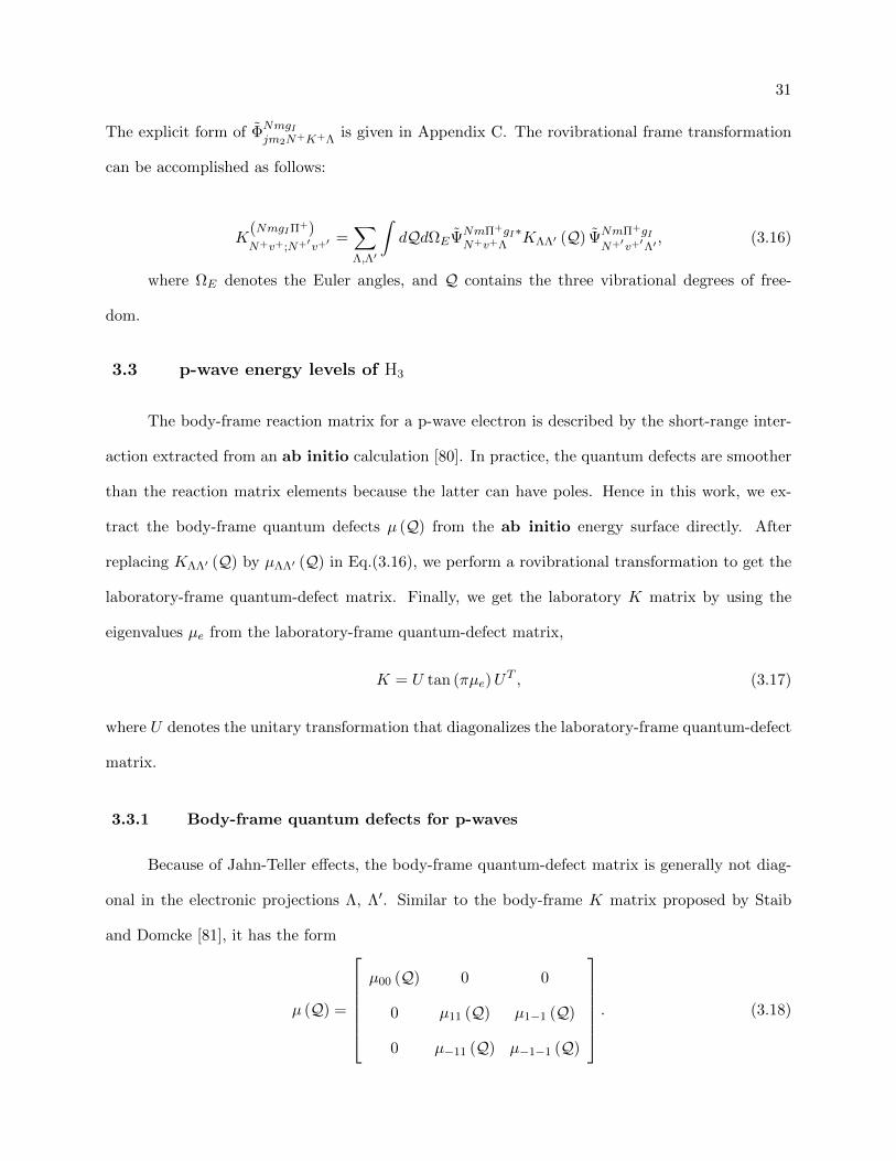
31

The explicit form of ΦNmgIjm2N+K+Λ

is given in Appendix C. The rovibrational frame transformation

can be accomplished as follows:

K(NmgIΠ+)N+v+;N+′v+′

=∑Λ,Λ′

∫dQdΩEΨNmΠ+gI∗

N+v+ΛKΛΛ′ (Q) ΨNmΠ+gI

N+′v+′Λ′, (3.16)

where ΩE denotes the Euler angles, and Q contains the three vibrational degrees of free-

dom.

3.3 p-wave energy levels of H3

The body-frame reaction matrix for a p-wave electron is described by the short-range inter-

action extracted from an ab initio calculation [80]. In practice, the quantum defects are smoother

than the reaction matrix elements because the latter can have poles. Hence in this work, we ex-

tract the body-frame quantum defects µ (Q) from the ab initio energy surface directly. After

replacing KΛΛ′ (Q) by µΛΛ′ (Q) in Eq.(3.16), we perform a rovibrational transformation to get the

laboratory-frame quantum-defect matrix. Finally, we get the laboratory K matrix by using the

eigenvalues µe from the laboratory-frame quantum-defect matrix,

K = U tan (πµe)UT , (3.17)

where U denotes the unitary transformation that diagonalizes the laboratory-frame quantum-defect

matrix.

3.3.1 Body-frame quantum defects for p-waves

Because of Jahn-Teller effects, the body-frame quantum-defect matrix is generally not diag-

onal in the electronic projections Λ, Λ′. Similar to the body-frame K matrix proposed by Staib

and Domcke [81], it has the form

µ (Q) =

µ00 (Q) 0 0

0 µ11 (Q) µ1−1 (Q)

0 µ−11 (Q) µ−1−1 (Q)

. (3.18)

32

We express each matrix element by using the vibrational symmetry coordinates Q = (Q1, Qx, Qy)

as

Q1 = f1√3

(∆r1 + ∆r2 + ∆r3) , (3.19)

Qx = f1√3

(2∆r3 −∆r2 −∆r1) , (3.20)

Qy = f (∆r1 −∆r2) . (3.21)

(3.22)

where f = 2.639 255 bohr−1 is a constant and ∆ri describe displacements of the nuclei from the

equilibrium geometry at which r12 = r23 = r31 = requi = 1.6504 a.u.. For example, ∆r1 = r23−requi.

(Qx, Qy) can be alternatively described by another pair of coordinates (ρ, φ) as Qx = ρ cosφ and

Qy = ρ sinφ. Q1 describes the symmetric stretch of the molecule, while (Qx, Qy) or (ρ, φ) describe

bends and the asymmetric stretch. These coordinates are very useful here for our Taylor expansion

of the body-frame quantum defects around an equilibrium position. We use the following forms,

µ00 (Q) = µ00 (Q = 0) + a1Q1 + a2Q21 + a3Q

31 + a4ρ

2, (3.23)

µ11 (Q) = µ−1−1 (Q) (3.24)

= µ11 (Q = 0) + b1Q1 + b2Q21 + b3Q

31 + δρ2,

and

µ1−1 (Q) = µ−11 (Q) = λρ. (3.25)

The form of our off-diagonal matrix elements µ1−1 (Q) and µ−11 (Q) differs from the usual adopted

form in Ref. [31] by a phase factor exp (±iφ). This different phase convention is due to the fact

that the usual adopted form was derived in a body frame that is rotated from our body frame by

φ/2. We develop the detailed proof in Appendix D. The effective quantum numbers are calculated

by diagonalizing the quantum defect matrix. This calculation gives,

νn,π1,2 (Q) = n− [µ11 (Q)± |µ1−1 (Q)|] , (3.26)

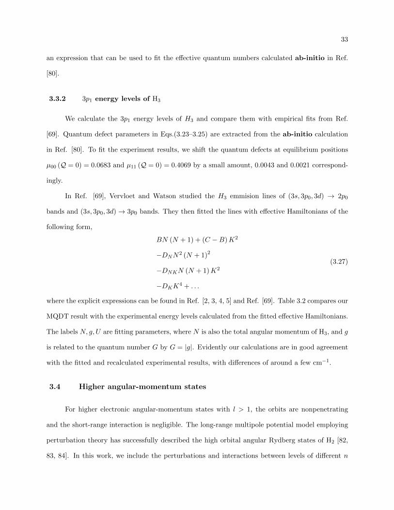
33

an expression that can be used to fit the effective quantum numbers calculated ab-initio in Ref.

[80].

3.3.2 3p1 energy levels of H3

We calculate the 3p1 energy levels of H3 and compare them with empirical fits from Ref.

[69]. Quantum defect parameters in Eqs.(3.23–3.25) are extracted from the ab-initio calculation

in Ref. [80]. To fit the experiment results, we shift the quantum defects at equilibrium positions

µ00 (Q = 0) = 0.0683 and µ11 (Q = 0) = 0.4069 by a small amount, 0.0043 and 0.0021 correspond-

ingly.

In Ref. [69], Vervloet and Watson studied the H3 emmision lines of (3s, 3p0, 3d) → 2p0

bands and (3s, 3p0, 3d)→ 3p0 bands. They then fitted the lines with effective Hamiltonians of the

following form,

BN (N + 1) + (C −B)K2

−DNN2 (N + 1)2

−DNKN (N + 1)K2

−DKK4 + . . .

(3.27)

where the explicit expressions can be found in Ref. [2, 3, 4, 5] and Ref. [69]. Table 3.2 compares our

MQDT result with the experimental energy levels calculated from the fitted effective Hamiltonians.

The labels N, g, U are fitting parameters, where N is also the total angular momentum of H3, and g

is related to the quantum number G by G = |g|. Evidently our calculations are in good agreement

with the fitted and recalculated experimental results, with differences of around a few cm−1.

3.4 Higher angular-momentum states

For higher electronic angular-momentum states with l > 1, the orbits are nonpenetrating

and the short-range interaction is negligible. The long-range multipole potential model employing

perturbation theory has successfully described the high orbital angular Rydberg states of H2 [82,

83, 84]. In this work, we include the perturbations and interactions between levels of different n

34

Table 3.2: A comparison between several of our calculated 3p1 H3 energy levels with empiricallyfitted experimental energy levels [2, 3, 4, 5].

Label1 Ecal2 Efit

3 Differences 4

N, g, U(cm−1

) (cm−1

) (cm−1

)0, 1, 1 12967.8 12966.863 0.91, 0, 1 12999.1 12998.196 0.91, 1, 1 13052.3 13050.966 1.31, 2, 1 13066.9 13068.700 -1.8

2, 0,−1 13139.9 13138.608 1.32, 1,−1 13056.1 13056.588 -0.52, 1, 1 13221.1 13219.125 1.92, 2, 1 13234.3 13235.522 -1.2

2,−3, 1 13203.8 13212.055 -8.33, 0, 1 13450.7 13446.072 4.6

3, 1,−1 13300.6 13300.119 0.53, 2,−1 13160.5 13165.030 -4.53, 2, 1 13485.4 13483.545 1.93, 3, 1 13453.2 13460.934 -7.7

aThe label denotes the values of N,G,U adopted in Ref. [69] to fit the experimental energy levels.bTheoretical results calculated in this study.cEmpirical fits for experimental energies determined in Ref. [69].dDifferences theory - experiment.

35

(principle quantum number) and l (angular-momentum quantum number) in a systematic fashion

by incorporating the formalism of MQDT [85]. We use this long-range model to calculate the

Rydberg states of H3 with l ≥ 2.

For a Rydberg electron with high orbital angular momentum (l ≥ 2 in the case of H+3 ), the

effects of core penetration are negligible. Hence, the interaction between the Rydberg electron

and the ion core can be approximately described by two effects. First, the interaction potential

between the Rydberg electron and the molecular ion is expanded into a multipole series, where the

quadrupole moment of the H+3 core is the leading anisotropic term. Second, the induced dipole

moment of the ion core interacts with the Rydberg electron by a potential characterized by the

polarizability of the H+3 core. All higher angular momenta and higher-order polarizabilities are

neglected here, as well as the anisotropic portion of the polarizability interaction.

In this approximation, the Hamiltonian is given in atomic units by

H = −1

2∇2 − 1

r+ Veff +Hcore, (3.28)

where Hcore is the rovibrational energy of the H+3 core. Veff includes quadrupole and polarizability

interactions:

Veff = Vquad + Vpol = −Q2

r3P2

(cos θ′e

)− α

2r4− γ

3r4P2

(cos θ′e

). (3.29)

where Q2, α, and γ are respectively the quadrupole moment, isotropic polarizability and the

cylindrically-symmetric anisotropic polarizability. Other components of the quadrupole moment

tensor vanish for the undistorted equilateral triangle configuration. For the vibrational ground

state, Q2, α, and γ are taken from table III of Ref. [86, 87]. The polarizability and quadrupole

interactions are much smaller than the Coulomb interaction and hence will be treated in perturba-

tion theory. We also find that the quantum defect is small (of the order of 0.01), and the coupling

between vibrational ground states of H+3 to excited vibrational states are negligible. Hence, in

the rovibrational transformation, we only include the vibrational ground state. The body-frame

reaction matrix thus can be written as

KΛΛ′ ≈ −π∫drfnl (r) 〈YlΛ|Veff |YlΛ′〉 fnl (r), (3.30)

36

Table 3.3: Comparison between several of our calculated 3d energy levels of H3 with experimentally-determined energy levels[2, 3, 4, 5].

Label1 Ecal2 Efit

3 Differences4

N+,K+, N(cm−1

) (cm−1

) (cm−1

)2, 1, 0 17399.14 17415.86 -15.892, 2, 0 17058.41 17039.61 18.801, 0, 1 17284.81 17296.57 -11.763, 0, 1 17742.32 17741.29 1.031, 1, 1 17005.99 16991.72 14.282, 1, 1 17403.89 17412.83 -8.943, 1, 1 17698.40 17700.43 -2.022, 2, 1 17107.24 17094.12 13.133, 2, 1 17540.96 17557.32 -16.353, 3, 1 17204.46 17188.48 15.981, 0, 2 17011.36 17001.08 10.273, 0, 2 17643.36 17655.58 -12.21

aThe label denotes the quantum numbers N+,K+, N .bTheoretical results calculated in this work.cEmpirical fits to the experimental energies determined in Ref. [69].dDifferences between theoretical and experimental results.

37

where fnl is the regular Coulomb function with l = 1 as the angular momentum quantum number

and n as the principal quantum number. As the quantum defect for d-wave electrons are small, we

can use integers for n in calculating the radial functions. Here, r is the electronic radial coordinate.

Again, we perform a rovibrational transformation (with only the vibrational ground states) to

obtain the laboratory-frame K matrix and finally, calculate the energy levels using the standard

determinantal equation of MQDT.

Table 3.3 compares our theoretical calculations with the experimentally-determined 3d energy

levels [69]. The agreement somewhat poorer than the p-wave case.

3.5 Recombination-pumped triatomic hydrogen infrared lasers

The nice comparisons between our calculated low-lying Rydberg energy levels and the exper-

iment results give us confidence of our method, and encourage us to apply it for higher Rydberg

states. In a recent experiment, mid-infrared laser lines observed in hydrogen/rare gas discharges

are assigned to three-body recombination processes involving an electron, a rare gas (He or Ne)

atom, and the triatomic hydrogen ion (H+3 ). Calculations of radiative transitions between higher

Rydberg states of neutral (H3) Rydberg states support this interpretation, and link it to recent

results for hydrogenic/rare gas afterglow plasmas. A mechanism for the population inversion is also

proposed in this section.

In this experiment [44], laser emission lines were produced from an ultrahigh finesse optical

supercavity containing a supersonically expanding plasma in the spectral range of 930 – 4370 cm−1,

with the majority occurring near 7 µm (1430 cm−1). The supersonic slit expansion generates a

weakly ionized plasma with neutral gas density expanding as the reciprocal of distance from the

slit nozzle, such that the pressure in the region of observation is in the range of 0.1 to 10 Torr

(densities of 1015 – 1017 cm−3). Fifty-seven laser transitions were observed in both H2 – He and

H2 – Ne gas mixtures. Twenty-nine laser transitions in H2 – He were also observed in H2O – He

or H2O – Ne discharges, which is not surprising, as these plasmas are known to produce significant

amounts of hydrogen [88].

38

It was found that laser intensity was highly dependent on partial pressure of H2 in the

expanding gas mixture, maximizing when the mixing ratio was < 1%. No lasing was observed

when pure H2 gas was used for the expansion. This most probably reflects the conversion of the

dominant H+3 ion to the H+

5 complex at higher hydrogen concentrations, as characterized by Glosik

et al [89].

To test whether contaminants such as O2 or H2O could be involved in the lasing observed in

the H2/He plasma, three experiments were performed. First, O2 was carefully added to the gas line

through a needle valve to determine how the presence of O2 affected laser intensity, revealing that

it decreased significantly when O2 was added to the gas mixture. Second, no lasing was observed

when the H2 cylinder was closed, indicating that the lasing species was indeed generated from the

cylinder gas. Third, in case the cylinder was itself contaminated with traces of condensible, the

gas was flowed through a long (∼8 ft) liquid nitrogen trap. No difference was observed in the

lasing intensity with or without the liquid N2 trap, indicating that the lasing species originates

from species produced from pure H2 and He or Ne.

We applied the long-range multipole potentialmodel discussed in the section 3.4 to the d-wave

Rydberg states of H3. While the d-wave Rydberg states of H3 were computed with this long-range

model, the p-wave Rydberg states are computed separately using the method discussed in section

3.3, since they are mainly dominated by the short-range interaction between the outer electron

and the ion core [90, 91]. These p-wave Rydberg states either autoionize or predissociate much

more rapidly than do the d-wave Rydberg states because of their stronger Jahn-Teller couplings,

or through ordinary l-uncoupling, which causes rotational autoionization and does not rely on the

Jahn-Teller effect. The corresponding d-p H3 dipole transitions thereby satisfy one of the golden

rules of astrophysical lasers, viz. the lifetime of the lower level of a lasing transition should be

much shorter than the lifetime of the upper level independent of the excitation mechanism;[] hence,

a population inversion can be created by the recombination process, and mid-IR lasing can occur

under proper conditions. Comparison of the measured lasing lines with the theoretical nd to np

lines suggests that metastable H3 created in the expanding plasma is indeed a likely candidate for

39

the carrier of these lasing transitions. Note, however, that the candidate lasing lines calculated

in this study are primarily of the type 4d–4p, whereas the ternary recombination mechanism is

believed to predominantly produce much higher Rydberg levels with principal quantum numbers

in the range n ≈ 40 ∼ 60 or even higher. This view of the process therefore requires a cascade, i.e.,

a decay of these highly excited nf levels to the 4d states, which then have a population inversion

and are able to lase while decaying to the 4p levels of H3.

Because there are no laboratory measurements of the 4d – 4p transitions that appear to

be the most likely candidates for the lasing lines reported here, the theoretical model has been

tested (in section 2.3 and 2.4) against the experimental 3d to 3p transitions of H3 that were

measured by Herzberg, showing good agreement (the rms error for 14 tabulated transitions is

below 13 cm−1) [92]. A comparison between the current experiment and our theoretical calculation

is shown in Fig. 3.2 and table 3.4. However, there are a few residual experimental lines having no

corresponding theoretical transition. These may correspond to Rydberg levels of the ion core with

other N+,K+, although we do not have specific candidates in mind at this point.

The conditions obtaining in the pulsed supersonic slit jet plasma used to generate the observed

IR laser action described here are similar to those employed by Glosik et al. in their studies of H+3

recombination in flowing afterglow plasmas [89, 93]. The total gas pressure drops from the 1 – 2

atmosphere nozzle backing pressure as the reciprocal of distance from the 300 – 400 µm wide exit

slit, yielding neutral gas densities of 1014 – 1017 cm−3 in the regions probed. Typical fractional

ionizations in such plasmas are ∼10−5. Studies of the H3O+ ion in similar pulsed slit jet discharges

yielded number densities near 1010 cm−3 and a rotational temperature near 110 K for this ion.

Glosik et al. measured the temperature-dependent recombination rate of H+3 with electrons in

recombination-limited He/Ar/H2 plasmas at He densities of 0.5 – 6 × 1017 cm−3 and temperatures

of 77 – 300 K. They identified three different behaviors of the measured recombination coefficient

with respect to hydrogen content. For [H2] < 1012 cm−3 (or <10−5 of the total gas density), it

increases with increasing H2 density and the spin states of H+3 are not equilibrated. For 1012 <

[H2] < 5 × 1013 cm−3, the rate is independent of H2 density and the ion is in thermal equilibrium.

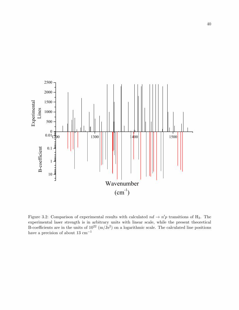
40

1200 1300 1400 15000

500

1000

1500

2000

2500

10

1

0.1

0.01

Expe

rimen

tal

Line

sB-coe

fficient

Wavenumber(cm-1)

Figure 3.2: Comparison of experimental results with calculated nd → n′p transitions of H3. Theexperimental laser strength is in arbitrary units with linear scale, while the present theoreticalB-coefficients are in the units of 1022 (m/Js2) on a logarithmic scale. The calculated line positionshave a precision of about 13 cm−1

41

Table 3.4: Possible assignment of laser lines observed in this work. We calculate the theory linesby using models described in this chapter. The experiment lines are chosen from the H2O – Helaser lines which are also observed in H2O – He or H2O – Ne experiments.

Initiala Finalb Theory H2O-He Differencec B/1021 H2O – HeN+,K+,N ,nd K+,N ,n′pλ lines(cm−1) lines(cm−1) (cm−1) (m/Js2) intensity

3,1,3,5d 1,2,5pπ− 1053.41 1054.63 1.22 2.26 1303,1,1,5d 1,2,5pπ− 1084.27 1082 -2.27 4.24 100

1218.47 3001,1,1,4d 1,2,4pπ+ 1231.06 1231.59 0.53 0.10 20001,1,3,4d 1,2,4pπ+ 1248.76 1249.37 0.61 3.71 7001,0,1,7d 0,1,6pπ 1256.36 1254.13 -2.23 0.08 110

1266.44 17003,1,3,6d 1,3,5pσ 1293.94 1297.83 3.89 961.95 14003,1,2,6d 1,3,5pσ 1302.57 1301.31 -1.26 0.44 6501,0,2,4d 0,2,4pπ 1312.78 1312.26 -0.52 6.28 8002,1,3,6d 1,2,5pσ 1316.66 1317.49 0.83 16.11 5001,1,1,6d 1,1,5pσ 1332.07 1332.05 -0.02 3.90 24002,2,3,6d 2,2,5pσ 1337.16 1336.66 -0.50 8.22 10002,1,3,7d 1,2,6pπ− 1346.83 1348.07 1.24 20.04 24002,1,1,7d 1,1,6pπ 1350.49 1349.14 -1.35 2.92 5002,2,2,4d 2,2,4pπ 1350.74 1349.85 -0.89 8.40 15001,0,3,4d 0,2,4pπ 1368.81 1367.29 -1.52 25.12 23003,1,4,7d 1,3,6pπ− 1370.69 1368.51 -2.18 2.34 24003,1,3,7d 1,3,6pπ− 1371.75 1371.18 -0.57 5.78 103,1,2,7d 1,3,6pπ− 1377.14 1375.35 -1.79 0.08 3002,2,3,4d 2,2,4pπ 1387.33 1385.87 -1.46 9.59 15001,1,1,4d 1,1,4pπ 1392.30 1392.6 0.30 8.12 401,1,1,4d 1,2,4pπ− 1399.42 1400.55 1.13 0.66 801,1,1,4d 1,1,4pπ 1392.30 1401.13 8.83 8.12 24001,1,1,4d 1,2,4pπ− 1399.42 1403.42 4.00 0.66 601,0,1,4d 0,2,4pπ 1411.91 1407.2 -4.71 0.70 10

1409.74 24001,1,3,4d 1,2,4pπ 1417.11 1418.84 1.73 23.93 2300

1421.09 24002,1,2,4d 1,2,4pπ+ 1439.63 1440.54 0.91 19.17 24001,1,2,4d 1,1,4pπ 1442.93 1444.22 1.29 14.62 5002,2,0,4d 2,1,4pπ 1445.25 1447.85 2.60 35.43 24001,0,2,4d 0,1,4pπ 1457.61 1455.45 -2.16 26.57 24002,1,1,4d 1,2,4pπ+ 1469.15 1462.08 -7.07 5.42 24002,2,1,4d 2,1,4pπ 1471.77 1472.73 0.96 26.57 1251,1,1,4d 1,0,4pπ 1475.02 1473.27 -1.75 19.68 2300

aThe initial states, labeled by the quantum number N+,K+, N, nd.bThe final states, labeled by the quantum number K+, N, n′pλ. An additional + or − denotes thepossible Jahn–Teller splitting of two p states: +(−) denotes the higher (lower) energy level.cThe difference between the theory lines and H2O – He laser lines.

42

For [H2] > 1013 cm−3, it again increases with increasing hydrogen density due to the conversion

of H+3 to the H+

5 complex [89], which recombines very rapidly, but which apparently does not

produce observable laser action in our experiments. Analysis of these data indicated that three-

body recombination processes dominated over two-body processes at pressures of a few Torr (1016 –

1017 cm−3) and temperatures near 300 K, and that this ternary rate maximizes at temperatures of

130 – 170 K. Hence, we can reasonably conclude that the three-body recombination processes also

dominate the ion loss in our recombination-limited supersonic plasmas. Glosik et al. [89, 93] show

that such processes are ca. 100 times faster than that previously described by Bates and Khare

[94], and they present a theoretical model for them. In this model, the resonant H+3 + e. complex

[i.e., the highly excited (n ≈40 – 60) H3 Rydberg molecule], which efficiently decays back into the

ion and electron via rotational autoionization, collides with a He atom during its lifetime, changing

the l-state of the complex to higher, longer-lived values. In particular, the l = 1(p) electronic states

are strongly coupled to the ion core and autoionize rapidly, whereas l ≥ 2(d) states are much more

longlived. These l-changing collisions of the H3 molecule thus produce the population inversion

required for the laser action observed in our experiments.

Glosik et al. have shown that in the low H+3 + e. collision energy regime, rotational excitation

of the vibrational ground state of the ion core with N+,K+ = 1, 1 produces long-lived Rydberg

states most efficiently. Hence, the most likely product immediately following collision would be a

highly excited (n ≈ 40 – 60) p-wave Rydberg electron attached to a N+,K+ = 2, 1 ion core.

A subsequent collision of the H3 neutral molecule with a rare gas atom changes the Rydberg

electron angular momentum to a longer-lived, higher value, and/or the collision of the He atom

with the H+3 core might deexcite the ion core, which would close the rotational autoionization decay

route. Radiative cascade can then populate the 4d levels that are the primary lasing candidates in

transitions to the 4p states. Hence, in the theoretical calculation, we include the transitions from

a 4d electron attached to 2, 1, 1, 1, and 1, 0 cores to the n→p energy levels of H3. Other

transitions of the type nf→nd and ng→nf of H3 have also been checked, but they do not appear to

be connected with the present experimental results.

43

3.6 Summary

In this chapter, we have calculated the Rydberg energy levels of H3 molecules. Using an

accurate ab-initio quantum-defect surface and ab-initio core energies of H+3 , our theoretical results

for the p-wave Rydberg states from the present MQDT calculations are in good agreement with

experimental results from J. K. G. Watson [69]. We also study higher-momentum states by a using a

long-range multipole potential model in conjunction with MQDT, and find encouraging agreement

with experimental results from Ref. [69]. Finally, applying such models for higher Rydberg states

gives supportive explanation of the mid-infrared laser lines in a recent experiment [44].

Chapter 4

Numerical study of three-body recombination

This chapter focus on another type of three-body systems: recombination of three particles

at ultracold temperature. Here, three-body recombination processes are treated numerically for

a system of three identical bosons. The two-body model potentials utilized support many bound

states, a major leap in complexity that produces an intricate structure of sharp nonadiabatic

avoided crossings in the three-body hyperradial adiabatic potentials at short distances. This model

thus displays the usual difficulties of more realistic systems. To overcome the numerical challenges

associated with sharp avoided crossings, the slow variable discretization (SVD) approach is adopted

in the region of small hyperradii. At larger hyperradii, where the adiabatic potentials and couplings

are smooth, the traditional adiabatic method suffices. Despite the high degree of complexity,

recombination into deeply bound states behaves regularly due to the dominance of one decay

pathway, resulting from the strong coupling between different recombination channels. Moreover,

the usual Wigner threshold law must be modified for excited incident recombination channels.

Note that the material in this chapter has been published in Ref. [95].

4.1 Introduction

Three-body recombination has attracted much theoretical and experimental research interest

in recent years. Recombination is the process in which three free particles collide to form a two-

body state and a free particle, with the released kinetic energy being distributed between the final

collisional partners. Such reactions are common and important in chemical reactions and in atomic,

45

molecular, and nuclear physics. In ultracold degenerate Fermi gases [96, 97, 98] recombination

has been used as a process to form weakly bound diatomic states, crucial for the experimental

realization of the BEC-BCS crossover physics. In fact, it was shown in Ref. [99] that the use of

recombination as an efficient way to produce weakly bound diatomic molecules can be extended

to systems other than fermionic gases. For colliding BECs at precisely-tuned relative velocity, the

formation of molecules via 3-body recombination can also be used to form molecules efficiently

owing to a double Bose enhancement [100]. Recombination processes normally release a high

amount of kinetic energy, producing atomic losses that often limit the lifetimes of Bose-Einstein

condensates (BEC) [101]. Moreover, three-body recombination has been recognized as one of the

most important scattering observables in which features related to the universal Efimov physics can

be manifested [102, 35, 103, 104, 32, 105]. Near a two-body Fano-Feshbach resonance, i.e., when the

s-wave scattering length a is much larger than the range r0 of the interactions, Efimov states can

occur, causing interference and resonant effects in recombination. The experimental observation of

these features in recombination has been recently used as evidence of Efimov physics in ultracold

quantum gases [106].

From the theoretical viewpoint, quantitative calculations of recombination for the typical

alkali atoms used in experiments in ultracold gases are limited by the large number of diatomic

states existing in such systems. Most of the available calculations for recombination for realistic

systems have been confined to model systems possessing just a few bound states and/or systems with

small scattering lengths, and even these are challenging calculations [107, 108, 47, 109]. As a result,

recombination calculations relevant for ultracold gases can only be made in the universal regime

|a| r0, by using simple potential models (with a few-bound states) or else by simply modeling the

decay into all deeply bound molecular states through a single inelastic parameter [104]. However,

in ultracold gases experiments the condition of universality is typically not satisfied, making it

desirable to perform more realistic calculations involving more sophisticated two-body models with,

eventually, a larger number of deeply bound states. This paper develops a methodology within the

hyperspherical adiabatic representation that permits the treatment of systems with many bound

46

states.

The present study still utilizes two-body potentials models that are, however, designed to

support many bound states, and therefore mimic three-body collisions for more realistic scenarios.

In the hyperspherical representation, the existence of many bound states leads to a complex set of

sharp nonadiabatic avoided crossings in the hyperspherical potential curves at short distances. The

large number of sharp avoided crossings creates numerical difficulties for the traditional adiabatic

representation as formulated with d/dR couplings [110]. To overcome these numerical difficulties,

one solution is to use the slow variable discretiazation (SVD) method proposed by Tolstikhin et

al [75]. The SVD method has been successfully applied to three-body bound-state calculations

[110, 63] and three-body collisions for the H + Ne2 system [111, 112]. Those calculations, however,

did not require numerical solution of the hyperradial equation [see Eq. (2.17) below] out to large

distances. To study ultracold collision processes such as recombination in the large scattering length

limit, it is crucial to solve the hyperradial equation out to very large distances. Since application of

SVD over the entire space is demanding in terms of memory and cpu-time, it is in fact much more

efficient to separate the domain of hyperradii into two regimes. At short distances, where many

avoided crossings appear, the SVD method is applied, while at large distances, where the adiabatic

potential curves are smooth, the traditional adiabatic method [54] is utilized.

This two-pronged strategy enables efficient calculation of the three-body recombination rate

at low collision energy, with extremely stable results for a two-body potential model supporting

up to about 10 bound states. This numerical capability of calculating recombination with many

bound states permits us to study the final state distribution of the recombination rate, K3. One

unexpectedly simple finding is that the branching ratio of recombination into a particular final (f)

channel, defined as

r(f←i)3 =

K(f←i)3∑

f

K(f←i)3

(4.1)

is the same for different initial (i) three-body collision channels. In the above equation, K(f←i)3

is the partial recombination from the initial three-body channel i to a particular final channel f .

47

The threshold laws for the partial recombination rates have also been considered, i.e., recombi-

nation processes occurring from excited three-body continua. These partial rates are observed to

deviate from the usual Wigner threshold law. Specifically, the energy dependence of the partial

recombination rates display a much weaker suppression than the usual Wigner analysis [113, 103]

for excited continuum channels. These numerical results can be interpreted as the manifestation

of a strong coupling between three-body continuum channels. This is further quantified through a

perturbation series expansion of the scattering matrix that reveals the three-body recombination

pathways at low collision energies.

This article is organized as follows. Section 4.2 discusses the numerical details in this study.

Section 4.3 shows the numerical results for the three-body recombination rates , and Section 4.4

presents our analysis of the recombination pathways. Section 4.5 summarizes and concludes.

4.2 Adiabatic hyperspherical representation

The system studied here consists of three identical bosons with masses m1 = m2 = m3 = m

with total angular momentum J = 0. The present study uses a two-body potential model in form

of

v (rij) = Dsech2

(rijr0

), (4.2)

where the coefficient D is negative, and its magnitude is chosen to be large enough to support 8

to 10 two-body bound states (4 to 5 s-wave bound states). The total interaction potential can be

approximated accurately by a pairwise sum of two-body interaction:

V (R, θ, ϕ) = v (r12) + v (r23) + v (r31) . (4.3)

The first correction to this expression, the Axilrod-Teller term [114], is included latter and found

unimportant. Using the numerical basis discussed in Ref. [47], Eq. (2.12) is solved for the adiabatic

potential and channel functions.

Figures 4.1 and 4.2 show the typical adiabatic potential curves for the parameterm = 7.2963×

103 a.u., D = −5.500× 10−5 a.u. and r0 = 15 a.u. Figure 4.1 exhibits several sharp nonadiabatic

48

avoided crossings at short distances. Although in our representation sharp crossings are associated

with vanishingly small transition probabilities, these avoided crossings can cause several numerical

difficulties when solving for the hyperradial motion in the traditional adiabatic approach. As

mentioned above, such difficulties are overcome by implementing the SVD method described in

Ref. [75]. Figure 4.2 shows, however, that the adiabatic potentials at long distances are smooth

and, therefore, are more suitable for traditional approaches. The R-matrix propagation method

was discussed in subsection 4.2.4 and Appendix B. With this method, R-matrix at very large

distance can be obtained. The scattering matrix S is then given by Eq. (2.22).

The three-body recombination rate is therefore given by [47]

K(f←i)3 =

192π2 (2J + 1)

µ3bk4|Sfi|2 , (4.4)

where Sfi is the appropriate S-matrix elements, J is the total angular momentum of the system,

and k =√

2µ3bE gives the hyperradial wave numbers in the incident channels.

4.3 Three-body recombination rates

The present numerical study focuses on systems of three identical bosons with total angular

momentum J = 0, with parameters adjusted to represent the 4He system (m1 = m2 = m3 =

7.2963× 103 a.u. and r0 = 15 a.u., the same as in Fig. 4.1). The two-body potential depth D [see

Eq. (4.2)] is adjusted to tune the scattering length a and explore both the positive- and negative-

scattering length cases while supporting 8-10 bound states. The recombination rate near the unitary

regime (k |a| ≈ 1), is explored next for two sets of typical parameters: D = −5.500× 10−5 a.u. for

the positive-scattering length case, a = 1020.36 a.u.; D = −5.467×10−5 a.u. for negative-scattering

length case, a = −1096.07 a.u. For both cases a is much larger than r0 (|a|/r0 ≈ 70) and therefore

such calculations are solidly within the universal regime [104, 103].

The black dashed lines in Figs. 4.1 and 4.2 denote the recombination channels, i.e., the

final state channels of the recombination process. The effective hyperradial potentials Uν (R) ≡

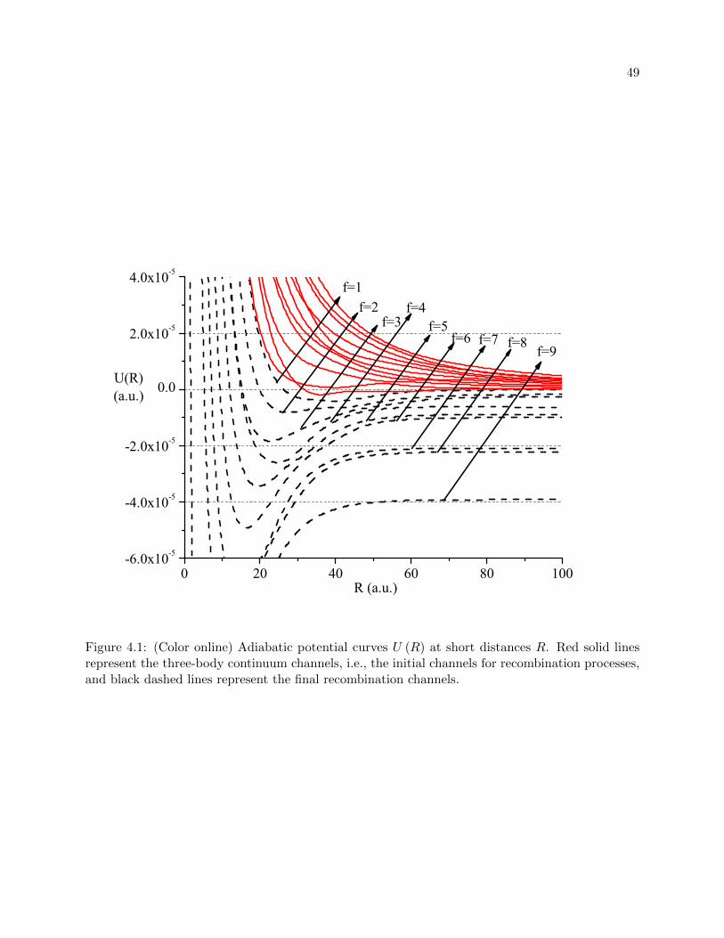
49

0 20 40 60 80 100-6.0x10-5

-4.0x10-5

-2.0x10-5

0.0

2.0x10-5

4.0x10-5

f=9f=8f=7f=6f=5

f=4f=3

f=2

U(R)(a.u.)

R (a.u.)

f=1

Figure 4.1: (Color online) Adiabatic potential curves U (R) at short distances R. Red solid linesrepresent the three-body continuum channels, i.e., the initial channels for recombination processes,and black dashed lines represent the final recombination channels.

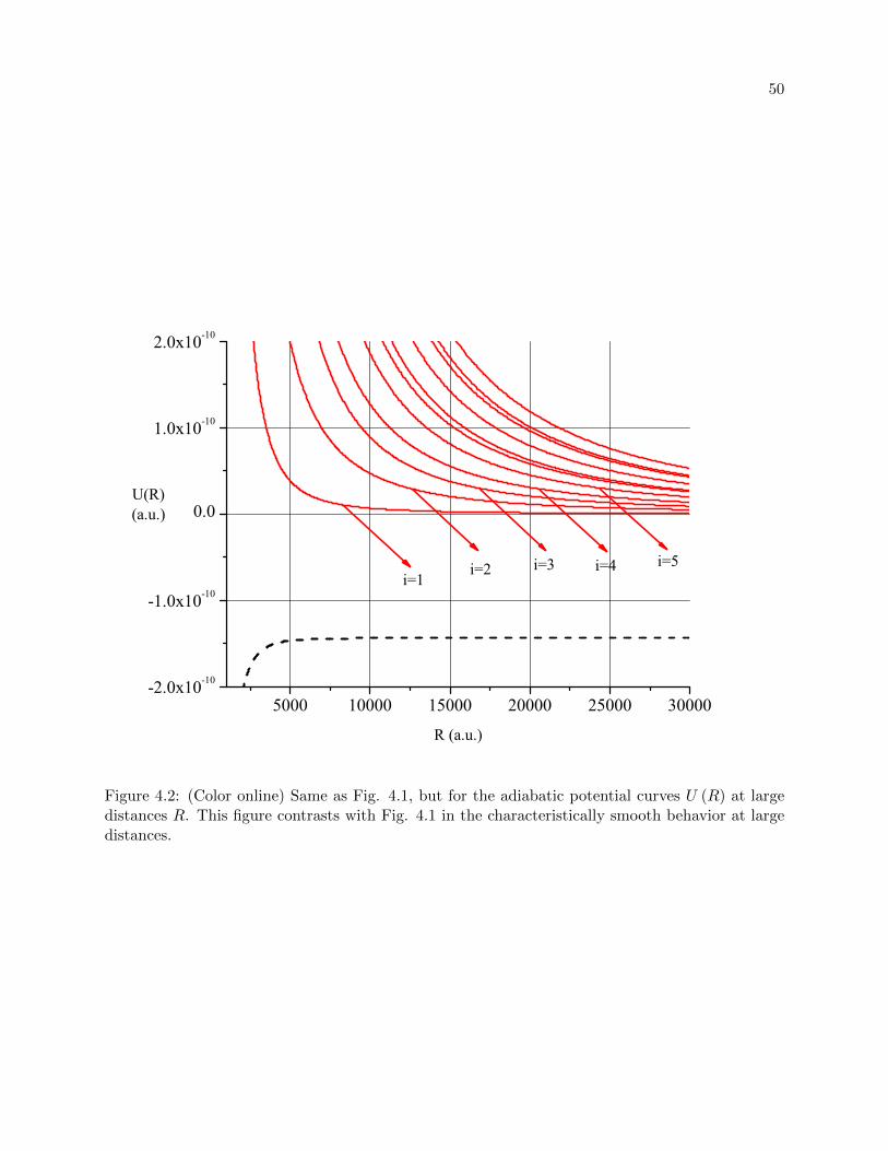
50

5000 10000 15000 20000 25000 30000-2.0x10-10

-1.0x10-10

0.0

1.0x10-10

2.0x10-10

i=5i=4i=3i=2

U(R)(a.u.)

R (a.u.)

i=1

Figure 4.2: (Color online) Same as Fig. 4.1, but for the adiabatic potential curves U (R) at largedistances R. This figure contrasts with Fig. 4.1 in the characteristically smooth behavior at largedistances.

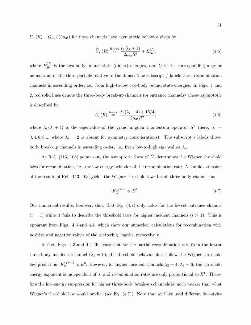
51

Uν (R)−Qνν/ (2µ3b) for these channels have asymptotic behavior given by

Uf (R)R→∞≈

lf (lf + 1)

2µ3bR2+ E

(f)2b , (4.5)

where E(f)2b is the two-body bound state (dimer) energies, and lf is the corresponding angular

momentum of the third particle relative to the dimer. The subscript f labels these recombination

channels in ascending order, i.e., from high-to-low two-body bound state energies. In Figs. 1 and

2, red solid lines denote the three-body break-up channels (or entrance channels) whose asymptotic

is described by

Ui (R)R→∞≈ λi (λi + 4) + 15/4

2µ3bR2, (4.6)

where λi (λi + 4) is the eigenvalue of the grand angular momentum operator Λ2 (here, λi =

0, 4, 6, 8..., where λi = 2 is absent for symmetry considerations). The subscript i labels three-

body break-up channels in ascending order, i.e., from low-to-high eigenvalues λi.

As Ref. [113, 103] points out, the asymptotic form of Ui determines the Wigner threshold

laws for recombination, i.e., the low energy behavior of the recombination rate. A simple extension

of the results of Ref. [113, 103] yields the Wigner threshold laws for all three-body channels as

K(f←i)3 ∝ Eλi (4.7)

Our numerical results, however, show that Eq. (4.7) only holds for the lowest entrance channel

(i = 1) while it fails to describe the threshold laws for higher incident channels (i > 1). This is

apparent from Figs. 4.3 and 4.4, which show our numerical calculations for recombination with

positive and negative values of the scattering lengths, respectively.

In fact, Figs. 4.3 and 4.4 illustrate that for the partial recombination rate from the lowest

three-body incidence channel (λ1 = 0), the threshold behavior does follow the Wigner threshold

law prediction, K(f←1)3 ∝ E0. However, for higher incident channels λ2 = 4, λ3 = 6, the threshold

energy exponent is independent of λi and recombination rates are only proportional to E1. There-

fore the low-energy suppression for higher three-body break-up channels is much weaker than what

Wigner’s threshold law would predict (see Eq. (4.7)). Note that we have used different line-styles

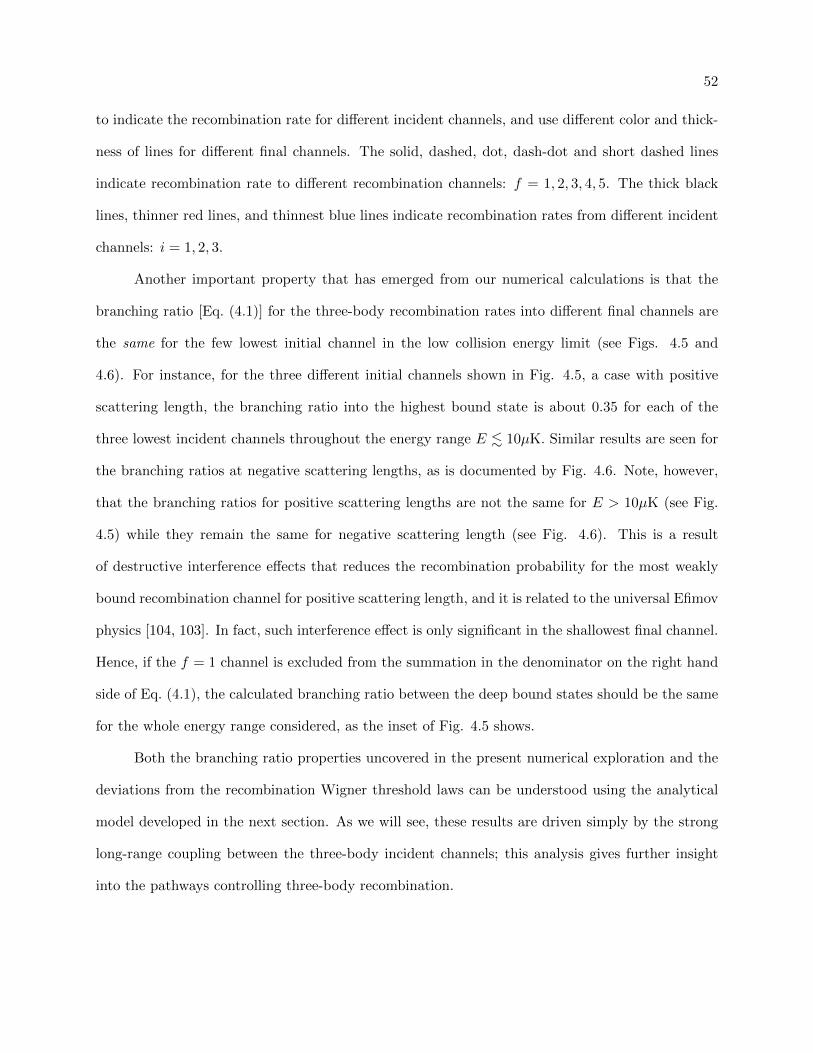
52

to indicate the recombination rate for different incident channels, and use different color and thick-

ness of lines for different final channels. The solid, dashed, dot, dash-dot and short dashed lines

indicate recombination rate to different recombination channels: f = 1, 2, 3, 4, 5. The thick black

lines, thinner red lines, and thinnest blue lines indicate recombination rates from different incident

channels: i = 1, 2, 3.

Another important property that has emerged from our numerical calculations is that the

branching ratio [Eq. (4.1)] for the three-body recombination rates into different final channels are

the same for the few lowest initial channel in the low collision energy limit (see Figs. 4.5 and

4.6). For instance, for the three different initial channels shown in Fig. 4.5, a case with positive

scattering length, the branching ratio into the highest bound state is about 0.35 for each of the

three lowest incident channels throughout the energy range E . 10µK. Similar results are seen for

the branching ratios at negative scattering lengths, as is documented by Fig. 4.6. Note, however,

that the branching ratios for positive scattering lengths are not the same for E > 10µK (see Fig.

4.5) while they remain the same for negative scattering length (see Fig. 4.6). This is a result

of destructive interference effects that reduces the recombination probability for the most weakly

bound recombination channel for positive scattering length, and it is related to the universal Efimov

physics [104, 103]. In fact, such interference effect is only significant in the shallowest final channel.

Hence, if the f = 1 channel is excluded from the summation in the denominator on the right hand

side of Eq. (4.1), the calculated branching ratio between the deep bound states should be the same

for the whole energy range considered, as the inset of Fig. 4.5 shows.

Both the branching ratio properties uncovered in the present numerical exploration and the

deviations from the recombination Wigner threshold laws can be understood using the analytical

model developed in the next section. As we will see, these results are driven simply by the strong

long-range coupling between the three-body incident channels; this analysis gives further insight

into the pathways controlling three-body recombination.

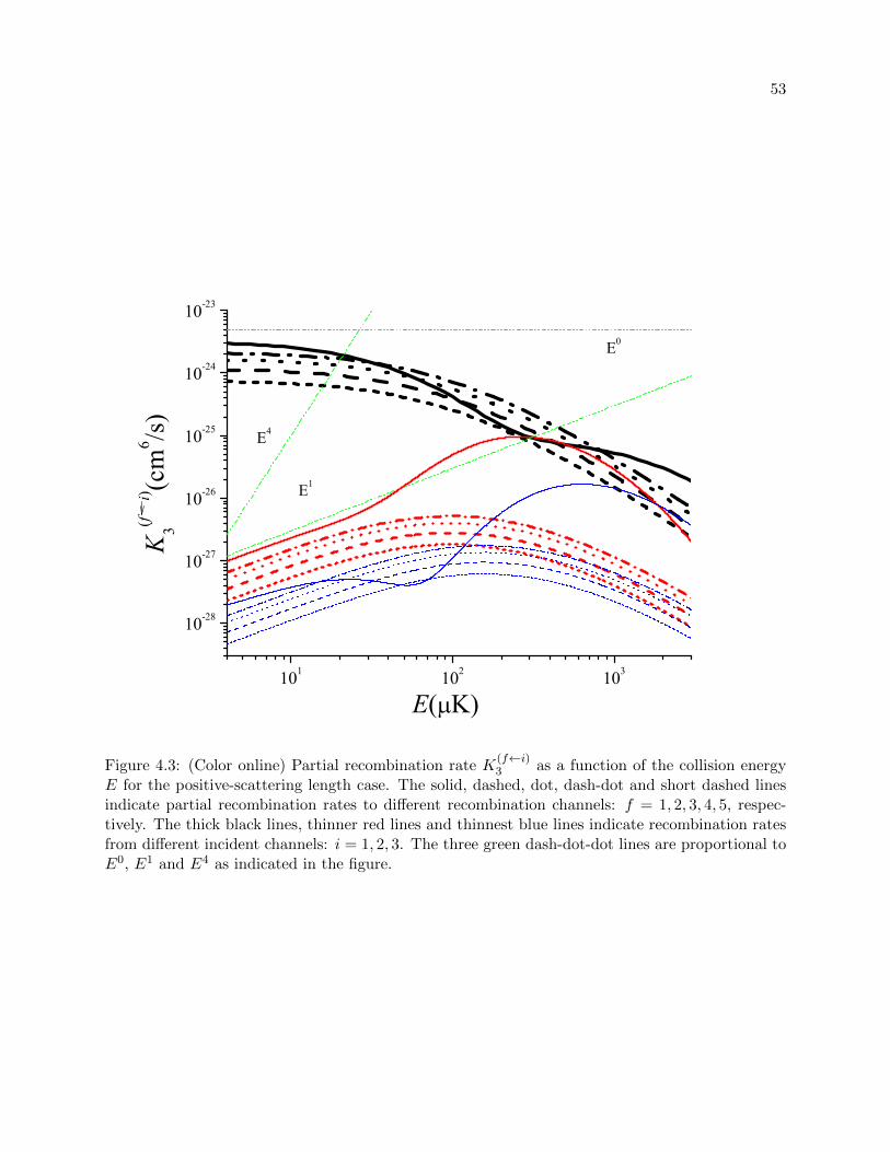
53

101 102 103

10-28

10-27

10-26

10-25

10-24

10-23

E4

E1

K3(f

i) (c

m6 /s

)

E( K)

E0

Figure 4.3: (Color online) Partial recombination rate K(f←i)3 as a function of the collision energy

E for the positive-scattering length case. The solid, dashed, dot, dash-dot and short dashed linesindicate partial recombination rates to different recombination channels: f = 1, 2, 3, 4, 5, respec-tively. The thick black lines, thinner red lines and thinnest blue lines indicate recombination ratesfrom different incident channels: i = 1, 2, 3. The three green dash-dot-dot lines are proportional toE0, E1 and E4 as indicated in the figure.

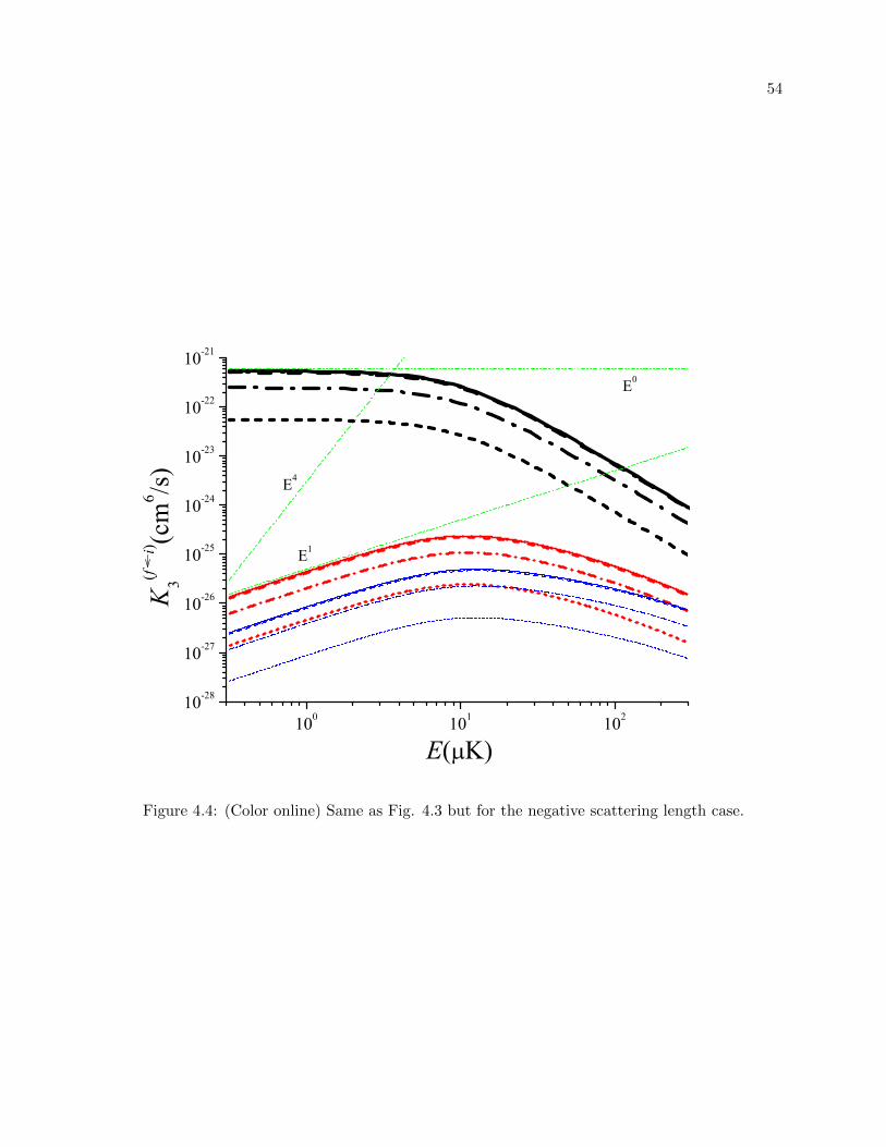
54

100 101 10210-28

10-27

10-26

10-25

10-24

10-23

10-22

10-21

E4

E1

E0

K3(f

i) (c

m6 /s

)

E( K)

Figure 4.4: (Color online) Same as Fig. 4.3 but for the negative scattering length case.

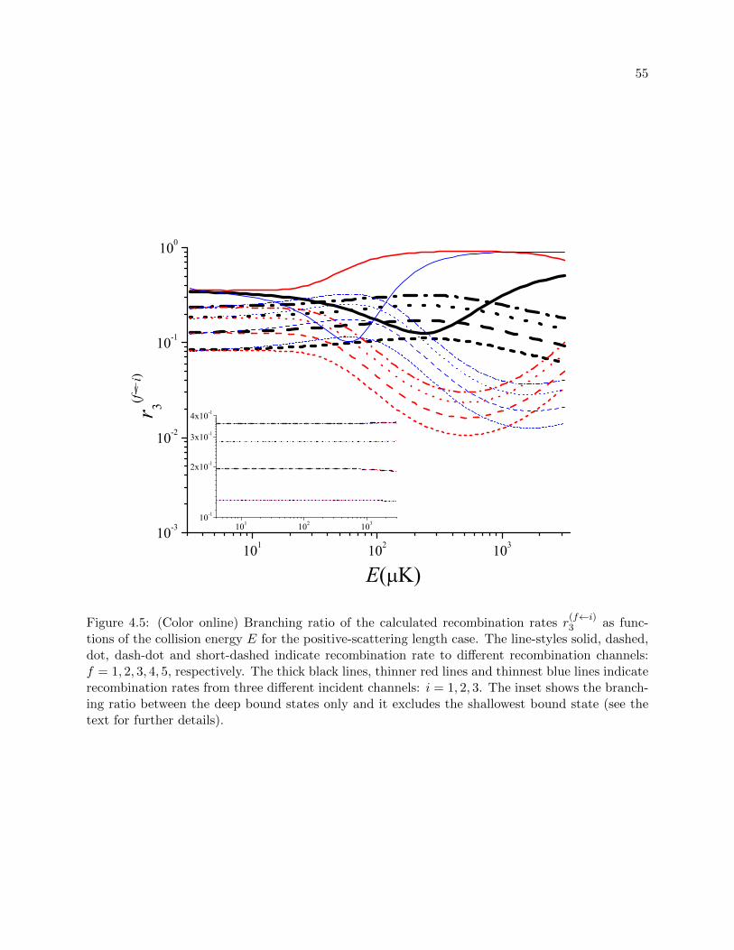
55

101 102 10310-3

10-2

10-1

100

101 102 10310-1

2x10-1

3x10-1

4x10-1

E( K)

r 3(f

i)

Figure 4.5: (Color online) Branching ratio of the calculated recombination rates r(f←i)3 as func-

tions of the collision energy E for the positive-scattering length case. The line-styles solid, dashed,dot, dash-dot and short-dashed indicate recombination rate to different recombination channels:f = 1, 2, 3, 4, 5, respectively. The thick black lines, thinner red lines and thinnest blue lines indicaterecombination rates from three different incident channels: i = 1, 2, 3. The inset shows the branch-ing ratio between the deep bound states only and it excludes the shallowest bound state (see thetext for further details).

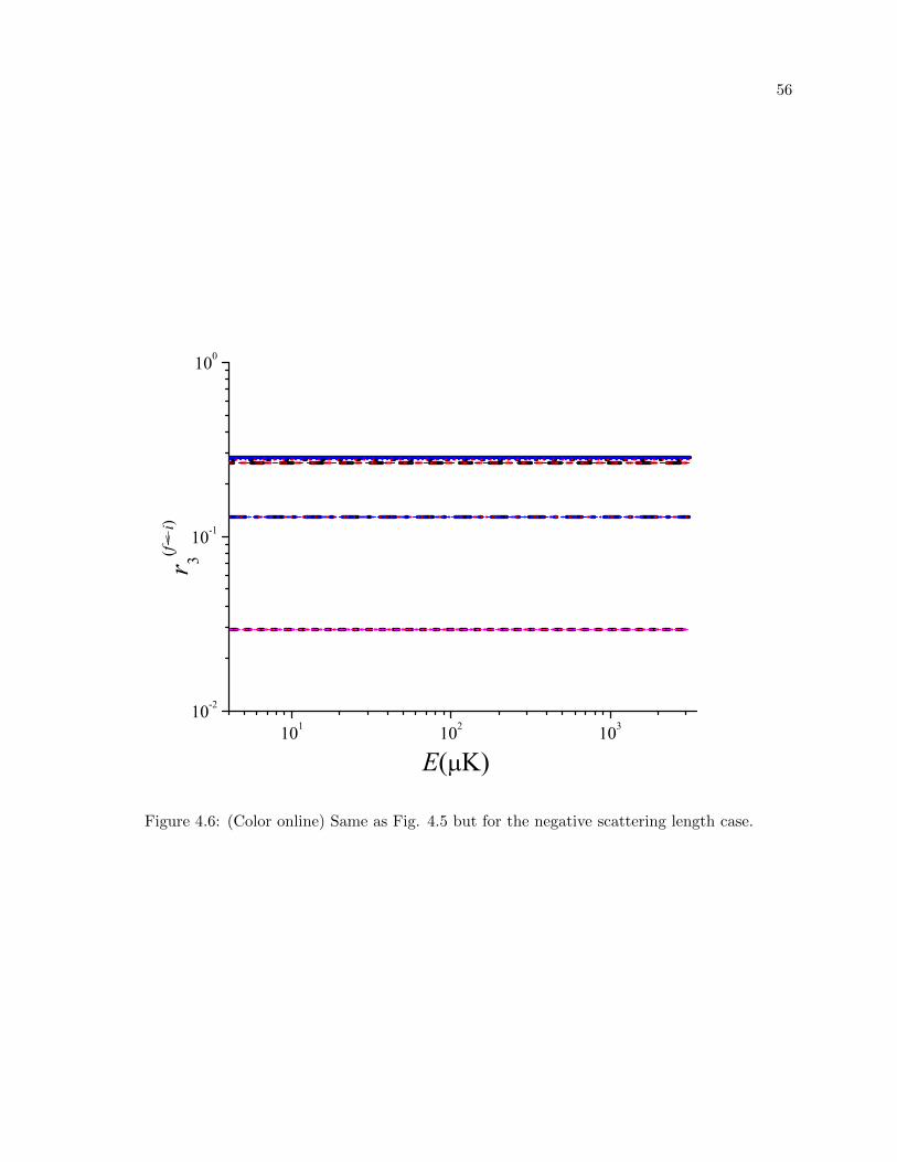
56

101 102 10310-2

10-1

100

r 3(f

i)

E( K)

Figure 4.6: (Color online) Same as Fig. 4.5 but for the negative scattering length case.

57

4.4 Dominant recombination pathways

The extensive numerical three-body recombination rates presented in the preceding section

are now interpreted in order to extract the important recombination pathways. Once these are

identified, the surprising low-energy threshold behavior and the branching ratio regularities cited

above become clear.

Our model consists of carrying out a perturbation expansion of the S-matrix and then as-

sociating each term to a specific pathway. As a first step, Eq. (2.17) is recast in matrix form

as

[TR +W − E1

]F = 0, (4.8)

where

(TR)µν = − 1

2µ3b

d2

dR2δµν (4.9)

and

Wνµ = Uνδνµ −1

2µ3b

[2Pνµ

d

dR+Qνµ

]. (4.10)

The off-diagonal terms of W are treated perturbatively, suggesting that the hyperradial Green’s

function matrix should be defined as the solution of

(TR + U − E1

)G(R,R′

)= δ

(R−R′

)1 (4.11)

where U is the diagonal submatrix of W , whose matrix elements coincide with Uν in Eqs. (4.5)

and (4.6). One can, therefore, write the hyperradial Green’s function as

G(R,R′

)= −πif (R<)h(+) (R>) , (4.12)

where f and h(+) are both diagonal matrices. The matrix elements of f are the solutions of Eq.

(4.11) regular at R = 0, and the outgoing Hankel solutions h are given by

h(+) (R) = f (R) + ig (R) , (4.13)

58

where g represent the corresponding irregular solutions. For the three-body break-up channels,

since the centrifugal barriers are dominant, the regular and irregular energy-normalized basis pair

fi and gi are well approximated in terms of Bessel functions as

fi (R) ≈√µ3bRJλi+2 (kR) , (4.14)

gi (R) ≈√µ3bRYλi+2 (kR) . (4.15)

The above hyperradial Green’s function can now be used to expand the S-matrix in a

distorted-wave Born series,

Sfi = S(0)fi + S(1)

fi + S(2)fi + ..., (4.16)

where

S(0)fi = δfi = 0, (4.17)

(f 6= i). In Eq. (4.16), the first order expansion of the scattering matrix element is simply given

by,

S(1)fi = 2πi

∫ ∞0

dRff (R)Wfi (R)fi (R) , (4.18)

and the low energy behavior of the S-matrix elements can be easily determined by inspection. The

integrand in Eq. (4.18) is only significant at small values of kR where fi (R) =√RJλi+2 (kR) ∝

kλi+2. Therefore,

S(1)fi ∝ k

λi+2. (4.19)

In terms of the pathways, the first order S-matrix element is the probability amplitude to transit

from the incident channel i and then tunnel through the centrifugal barrier and scatter into recom-

bination channels at short distances (R ∝ r0). Therefore, if the recombination process were solely

described by this pathway, the low energy behavior of recombination would be given by

K(f←i)3 =

192π2 (2J + 1)

µ3bk4

∣∣∣S(1)fi

∣∣∣2 ∝ k2λi = Eλi , (4.20)

recovering the usual threshold laws from Wigner’s analysis [113, 103].

59

The first-order result shown in Eq. (4.20) for the low energy behavior of recombination fails,

however, to explain our numerical coupled-channel results [see Figs. 3 and 5] implying that high

order perturbation terms in Eq. (4.16) are crucial in order to determine the actual threshold laws.

Hence we consider the second order partial-wave Born expansion, given by

S(2)fi = −2π2 (I1 + I2) , (4.21)

where,

I1 =∑

m 6=i 6=f

∫ ∞0

dRff (R)Wfm (R) fm (R)

×∫ ∞R

dR′h(+)m

(R′)Wmi

(R′)fi(R′), (4.22)

I2 =∑

m 6=i 6=f

∫ ∞0

dRff (R)Wfm (R)h(+)m (R)

×∫ R

0dR′fm

(R′)Wmi

(R′)fi(R′). (4.23)

The first integral I1 describes the quantum amplitude for a pathway in which the system

coming inward in incident channel i to first scatter into an intermediate state m via a long-range

coupling and then scatters to the final channel f at short distances. I2 describes the amplitude for

a different second-order pathway for which the system first scatters into an intermediate state m

at short distances and then scatters into the final channel f in a second step. Accordingly in our

analysis, the most important pathway for all incident channels is the one associated with the I1

term in Eq. (4.21), i.e., the pathways incorporated in I2 are much more strongly suppressed in the

low-energy limit.

Interestingly, the second-order correction for the S-matrix element associated with the lowest

three-body incidence channel (i = 1) can only be associated with an intermediate state (m) which is

a deeply-bound molecular channel or else an excited three-body continuum channel. In both cases,

our analysis shows that these contributions are unimportant in the low-energy limit. Therefore,

the threshold law for the lowest three-body channel is still given by Eq. (4.20) [with i = 1, λ1 =

60

0]. For recombination events starting from excited three-body channels (i > 1), however, the

situation is different. In this case the dominant pathway is the one that involves the lowest three-

body continuum channel as an intermediate channel (m = 1), with a corresponding second order

correction:

S(2)fi ≈ −2π2

∫ ∞0

dRff (R)Wf1 (R) f1 (R)

×∫ ∞R

dR′h(+)1

(R′)W1i

(R′)fi(R′). (4.24)

The long-range coupling W1i between the lowest three-body break-up channel and a higher incident

channel is dominated by the P-matrix element between the two channels. For different i > 1, the

P-matrix element P1i follows the same asymptotic behavior [54]

P1i (R) ∝ 1

R2, (R→∞) . (4.25)

Using the above equation and definition of Wνµ in Eq. (4.10), the integral in the second line of Eq.

(4.24) has the property that ∫ ∞R

dR′h(+)1

(R′)W1i

(R′)fi(R′)∝ k. (4.26)

The integral in the first line of Eq. (4.24) is the same as Eq. (4.18). Therefore, the second-order

scattering-matrix element for the i > 1 three-body break-up channels follows

S(2)if ∝ k

λ1+2k = k3, (4.27)

which is larger than the first-order S-matrix for channels i > 1 in the small k limit [see Eq. (4.19)].

Therefore, based on the discussions above, the threshold behavior of the partial recombination rate

for any incident channel can be summarized as

K(i←f)3 ∝

E0, i = 1,

E1, i > 1,

(4.28)

which is consistent with our numerical results shown in Figs. 3 and 5.

61

The present analysis, therefore, demonstrates that the important recombination pathway

for excited three-body incidence channels involves an intermediate transition to the lowest three-

body incidence channel, controlled by a strong and long-range coupling between continuum channels

[Eq. (4.25)]. This recombination pathway also explains why the relative recombination rate to reach

the same final recombination channel from different incident three-body channels is the same. For

ultracold collisions triggered from every excited three-body incidence channel (i > 1), our analysis

shows that the final state contribution for recombination is mainly controlled by the coupling

between the lowest three-body break-up channel at short distances. Therefore, the corresponding

relative final state contribution are independent of the initial excited three-body channel.

4.5 Summary

The methodology elaborated in this chapter is capable of calculating recombination rate

and, similarly, any other three-body scattering observable for systems that possess many two-body

bound states. Our numerical study was performed for systems with up to 10 bound states, but it

can be extended to larger problems with a good level of accuracy. Although our calculations for

larger systems might be limited by memory usage and CPU time, our approach still allows for the

analysis of increasingly more complex systems.

A key outcome is an understanding of the modified threshold laws for partial channel con-

tributions to three-body recombination of three identical bosons with angular momentum J = 0.

Our analysis for the important recombination pathways reveals that the threshold behavior of

the recombination rate for excited three-body incidence channels is significantly less suppressed at

low energy than a simple generalization of the Wigner’s threshold laws predicts. In addition, the

branching ratio of recombination into any given final state f is found to be the same for different

incident channels.

Chapter 5

Origin of the Three-body Parameter Universality in Efimov Physics

Three-body recombination has been recognized as one of the most important scattering ob-

servables in which features related to universal Efimov physics can be manifested. This chapter

focuses on studies of Efimov physics for a ≤ 0. The field-free recombination rate at the negative

site has an a4 scaling plus some resonance features. These resonances, as was pointed out initially

by [35], are closely related with the Efimov states. In principle, there are an infinite number of

these resonances corresponding to the infinite expected number of Efimov states. In addition, the

ratio between the positions of nearby resonances are universal, i.e., the ratio does not depend on

the details of the short-range two- and three-body interactions. This fact implies that all resonance

positions can be determined solely by a single parameter, known in the literature as the “three-body

parameter”. While previous fundamental assumptions in the theory of the Efimov effect suggest

that the three-body parameter should not be universal, recent experiments support the opposite

conclusion. The theoretical investigation in this chapter resolves this apparent contradiction by

elucidating the unanticipated implications of two-body interactions. Our study shows that the

three-body parameter universality emerges because a universal effective barrier in the three-body

potentials prevents the three particles from simultaneously getting close to each other. Our results

also show the limitations on this universality; it is more likely to occur for neutral atoms and less

likely to extend to light nuclei.

Note that the material in this chapter has recently been published [115], and some of the text

is adapted from that publication almost verbatim.

63

5.1 Introduction

Efimov physics was discovered by V. Efimov in the 1970’s [26]. He predicted that when the

two-body s-wave scattering length a→∞, there would be an infinite number of three-body bound

states for a system consisting of three identical bosons. The energies of these three-body states

obey the simple relation:

Ek+13b /Ek3b = exp (−2π/s0), (5.1)

where the integer k denotes the energy levels in ascending order. The geometric scaling factor

exp (π/s0) ≈ 22.7 is universal, i.e., it does not depend on the details of the two-body interaction

nor additional three-body forces as long as both two- and three-body interactions are shortrange.

Equation (5.1) implies that we only need to know one additional “three-body parameter” to

determine the absolute values of all the weakly bound Efimov spectra. One of the most fundamental

assumptions underlying our theoretical understanding of this peculiar effect is that this three-body

parameter should encapsulate all the details of the interactions at short distances [33]. For this

reason, the three-body parameter has been viewed as nonuniversal since its value for any specific

system would depend on the precise details of the underlying two- and three-body interactions

[116, 117, 118]. Indeed, in nuclear physics, this picture seems to be consistent, i.e., three-body

weakly bound state properties seem to be sensitive to the nature of the two- and three-body short-

range interactions [117]. However, a recent experiment in ultracold atomic gases to study Efimov

effects gives the opposite conclusion: the three-body parameter is universal for several different

alkali atomic species.

Although the universality of the geometric scaling factor implies that the Efimov physics

can be observed in any system consisting of three identical bosons, ultracold atom gases provide

a perfect playground because of the extraordinary degree of control for such systems. One of the

key experimental tools is to use a Fano-Feshbach resonance to magnetically tune the scattering

length [119]. Tuning the scattering length a from infinity to finite and negative, but still much

larger than the interaction range r0, the Efimov energies cross the three-body threshold one by

64

one at some scattering length a−k (corresponding to the kth Efimov state) and cause resonances in

the three-body recombination. The resonance positions also obey a simple relation: a−k+1/a−k =

exp (π/s0). People usually use a−3b ≡ a−0 corresponding to the Efimov ground state as the three-

body parameter. Equivalently, the Efimov ground state energy E03b or the corresponding wave

number κ∗ =(ma

∣∣E03b

∣∣ /~2)1/2

, where ma is the atomic mass, can also be used as the three-body

parameter.

Recently, Berninger et al. measured a−3b near four different Fano-Feshbach resonances with

ultracold atomic gases of 133Cs. Even though the short-range physics was expected to vary from

one resonance to another, Efimov resonances were found for values of the magnetic field at which

a=a−3b=−9.1(2)rvdW, where rvdW is the van der Waals length [120].1 Therefore, in each of these

cases, the three-body parameter was approximately the same, thus challenging a fundamental

assumption of the universal theory. Even more striking is the observation in Ref. [6] that the Efimov

resonance positions obtained for 39K [7],2 7Li [8, 9, 10], 6Li [11, 12, 13, 14], and 85Rb [15] are also

consistent with values of a−3b/rvdW found for 133Cs. These observations provide strong evidence

that the three-body parameter has a universal character for spherically symmetric neutral atoms,

therefore suggesting that something else beyond the universal theory needs to be understood.

5.2 Van der Waals interaction and classical suppression

Our theoretical model for two-body interactions mimics the tunability of the interatomic

interactions via Fano-Feshbach resonances by directly altering the strength of the interparticle in-

teractions and, consequently, leads to the desired changes in a. A Fano-Feshbach resonance is

fundamentally a multichannel problem. However, for a broad resonance that is open-channel dom-

inated, a single channel potential with van der Waals tail is a very good approximation [119]. This

work considers various model interactions to test the universality of our three-body calculations.

1 The van der Waals length is defined as rvdW ≡ (2µ2bC6/~2)1/4/2 where C6 is the van der Waals coefficient andthe two-body reduced mass µ2b. Note also that in Ref [6] the results were quoted in terms of the mean scatteringlength a ≈ 0.9556rvdW as defined in Ref. [120].

2 Here, we are speculating that the feature observed in this experiment at a = −11.02 a.u. might in fact bea three-body resonance, instead of a four-body resonance. The possibility of such a reassignment is by no meansproven, of course, and can only be answered through additional experimental studies.

65

The models we have used for the two-body interactions are:

vsch(r) = −Dsech2 (r/r0) , (5.2)

vaλ(r) = −C6r6

(1− λ6/r6

), (5.3)

vbλ(r) = −C6r6

exp(−λ6/r6

), (5.4)

vhsvdW(r) = BhsΘ (rhs − r)− C6

r6Θ (r − rhs) . (5.5)

The potential model in Eq. (5.2) is the modified Poschl-Teller potential, where D determines the

potential depth. Equation (5.3) is the usual Lennard-Jones potential, and Eq. (5.4) is a dispersion

potential with a soft wall at short range. In Eq. (5.5), Θ(x) the step-function [Θ(x) = 0 for x < 0

and 1 elsewhere. In practice, however, we have used a smooth representation of the step-function

Θ in order to simplify our numerical calculations.] The potential in Eq. (5.5), therefore, consists

of a hard-sphere potential for r < rhs (Bhs C6/r6hs) and a long-range dispersion −1/r6 potential

for r > rhs. In the present study, the parameters D and λ in Eqs. (5.2)–(5.4) are adjusted to give

the desired a and number of bound states. For convenience, we denote the values of D and λ at

which there exist zero-energy bound states (|a| → ∞) as D∗n and λ∗n, where n corresponds to the

number of s-wave bound states. For the potential model in Eq. (5.5), however, we adjusted rhs

to produce the changes in a, but we only performed three-body calculations near the first pole at

rhs ≈ 0.8828rvdW. While vsch(r) is usually used to mimic the interaction potential between nuclei,

potentials with van der Waals tails are very good models for interaction between neutral atoms.

5.2.1 Van der Waals interaction

One of the important properties of atomic gases is that the long-range two-body interaction

between two neutral atoms can be very well described by a van der Waals interaction: V2b (r) →

−C6/r6, where r is the interatomic distance. The asymptotic parameter C6 is known quite well for

most atomic pairs of interest, and determines the van der Waals length rvdW =(2µ2bC6/~2

)1/4/2,

where µ2b is the two-body reduced mass. A corresponding energy scale EvdW = ~2/(2µ2br

2vdW

),

called van der Waals energy, can also be defined. In general, when r rvdW, the interaction is

66

described by the asymptotic van der waals interaction; when r rvdW, V2b (r) is dominated by

complicated short-range physics.

Flambaum et al. have shown that, for a short-range potential well with a −Cm/rm tail (where

m are integers), the low-energy two-body scattering properties have some “universal” features,

providing that the short-range potential is “deep” enough to enable one to use semiclassical (or

WKB) approximation within the potential well [121, 120]. In this case, the s-wave scattering length

a and effective range reff are related by

reff = Fm −Gma

+Hm

a2, (5.6)

where Fm, Gm, and Hm only depend on the characteristic length scale rm =(2µCm/~2

)1/(m−2)/2

(r6 ≡ rvdW for van der Waals potential) and ν = 1/ (m− 2):

Fm =4

3

π

sin νπν2ν Γ (ν) Γ (4ν)

[Γ (2ν)]2 Γ (3ν)rm, (5.7)

Gm =16

3

π

sin νπν4ν Γ (1− 2ν) Γ (4ν)

νΓ (ν) Γ (2ν) Γ (3ν)r2m, (5.8)

Hm =16

3

π

sin νπν6ν Γ (1− 3ν) Γ (1− ν) Γ (4ν)

ν2 [Γ (ν)]2 [Γ (2ν)]2r3m. (5.9)

Equation (5.6) implies that the relation between effective range and scattering length only depends

on the long-range behavior of the potential and does not depend on the complicated short-range

physics. In another word, the relation is “universal”. For a van der Waals potential, the effective

range can be expressed as,

reff ≈ rvdW

[2.78946− 5.33333

rvdW

a+ 5.09856

(rvdW

a

)2]. (5.10)

In particular, at the pole a→∞, the effective range approximately equals to 2.78946 rvdW.

5.2.2 Classical (WKB) Suppression

The universal relation between effective range and scattering length for potentials with van

der Waals tails relies on the fact that the two-body zero-energy wave function at short-range can be

well described by the WKB approximation. When the short-range potential well is deep, the WKB

67

approximation becomes very good, and the zero-energy wave function amplitude at short distances

becomes very small. This WKB suppression could derive from the usual classical suppression (or

WKB suppression) of the probability for two particles to exist between r and r+dr in regions of high

local velocity ~kL(r), which is proportional to [~kL(r)/mdr]−1 (m being the particle mass), the

time spent in that interval dr. It is possible that there could be an additional suppression as well,

through quantum reflection from a potential cliff [122]. Systems supporting many bound states,

such as the neutral atoms used in ultracold experiments with their strong van der Waals attraction,

clearly exhibit this suppression. In general, a finite-range two-body potential that supports many

bound states decreases steeply with decreasing interparticle distance r, starting when r/rvdW . 1,

at which point the potential cliff plays a role analogous to a repulsive potential for low-energy

scattering. As will be seen latter, the origin of the universality of the three-body parameter is also

related to the suppression of the probability of finding two particles at distances r < rvdW. This

suppression at the two-body level is studied here with different numerical models.

The first two-body model utilized in this chapter is the Lennard-Jones potential vaλ. Figure

5.1 shows three Lennard-Jones potentials with λ = λ∗2, λ∗3, λ∗4 so that the 2nd, 3rd and 4th s-wave

bound states are exactly at the threshold, and a→∞ for all the three cases. It is clear that these

potentials agree with −C6/r6 for r rvdW and are very different at short distances r rvdW. The

inset shows the corresponding zero-energy wave functions. The wave functions again agree with each

other at large distances and differ at short distances. However, the differences at short distances

are very small, mainly because the wave function amplitude itself is very small. The amplitude

of the zero-energy wave function at short-range becomes small because of classical suppression.

Next, a detailed quantitative study of the suppression is carried out with all the model potentials

in Eqs. (5.2)–(5.5).

The potential models in Eqs. (5.3)–(5.5) have in common the same large r behavior given

by the van der Waals interaction with the characteristic length scale rvdW. Therefore, in order to

compare the results from these models to those for vsch, we define an equivalent rvdW for vsch through

the relationship between rvdW and the effective range reff for vsch, namely, rvdW ≈ reff/2.78947

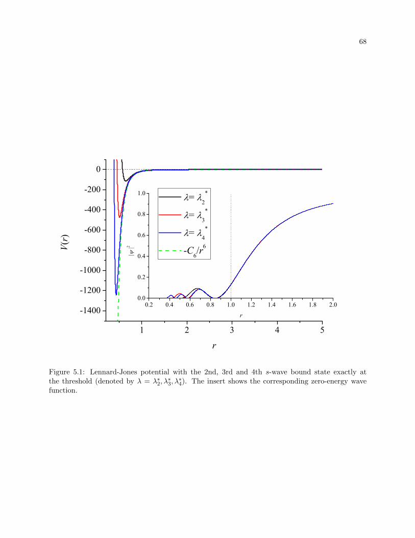
68

1 2 3 4 5

-1400

-1200

-1000

-800

-600

-400

-200

0

V(r)

r

= 2

*

= 3

*

= 4

*

-C6/r6

0.2 0.4 0.6 0.8 1.0 1.2 1.4 1.6 1.8 2.00.0

0.2

0.4

0.6

0.8

1.0

| |2

r

Figure 5.1: Lennard-Jones potential with the 2nd, 3rd and 4th s-wave bound state exactly atthe threshold (denoted by λ = λ∗2, λ

∗3, λ∗4). The insert shows the corresponding zero-energy wave

function.

69

[121, 120], which is valid for values of |a| r0. In fact, for vsch we have found that reff(|a| = ∞)

strongly depends on the potential depth D∗n (shown in Fig. 5.2), while for van der Waals type of

interactions, such as those in Eqs. (5.3)-(5.5), reff is fixed by reff ≈ 2.78947(2µ2bC6/~2)1/4/2.

Next we explore the origin of this suppression at the two-body level with these model poten-

tials. To gain some insight into the likelihood of finding particles inside the potential well, we start

by defining the following quantities,

ξinp (k) =

1

r0

∫ r0

0|ψk(r)|2dr, (5.11)

ξoutp (k) = lim

r→∞

1

r − r0

∫ r

r0

|ψk(r)|2dr, (5.12)

where ψk(r) is the two-body scattering wave function at energy E2b = k2/2µ2b, defined such that

ψk(r)r→∞

=sin(kr + δ)

sin δ, (5.13)

with δ ≡ δ(k) being the s-wave scattering phase shift. This definition for ψk(r), therefore, leads

to a zero-energy (k → 0) wave function of the form: ψ0(r) = 1 − r/a. [Note that in the above

equations r0 is the characteristic range of the two-body interaction. For the potential model in

Eq. (5.2), r0 is just the quantity in the argument of the sech function, while for the potential

models in Eqs. (5.3)–(5.5) it is defined to be r0 = rvdW].

The parameters ξinp and ξout

p can be associated with the “average” amplitude of the wave

function inside and outside the potential well, respectively. The amplitude inside the well relative

to the amplitude outside the well is therefore defined as:

ξrelp (k) =

ξinp (k)

ξoutp (k)

= 2 ξinp (k) sin2 δ. (5.14)

This relative amplitude vanishes in the limit k → 0 (sin δ ≈ −ka) as a result of our choice for

the asymptotic solution in Eq. (5.13), except at |a| = ∞, when δ is an odd multiple of π/2. The

quantity ξinp (k), however, remains finite in the k → 0 limit. Accordingly, this analysis suggests

that ξinp (k → 0) is the most relevant parameter for our analysis of the suppression inside the well.

Rigorously speaking, ξinp is not a probability, but it does measure the likelihood of finding two

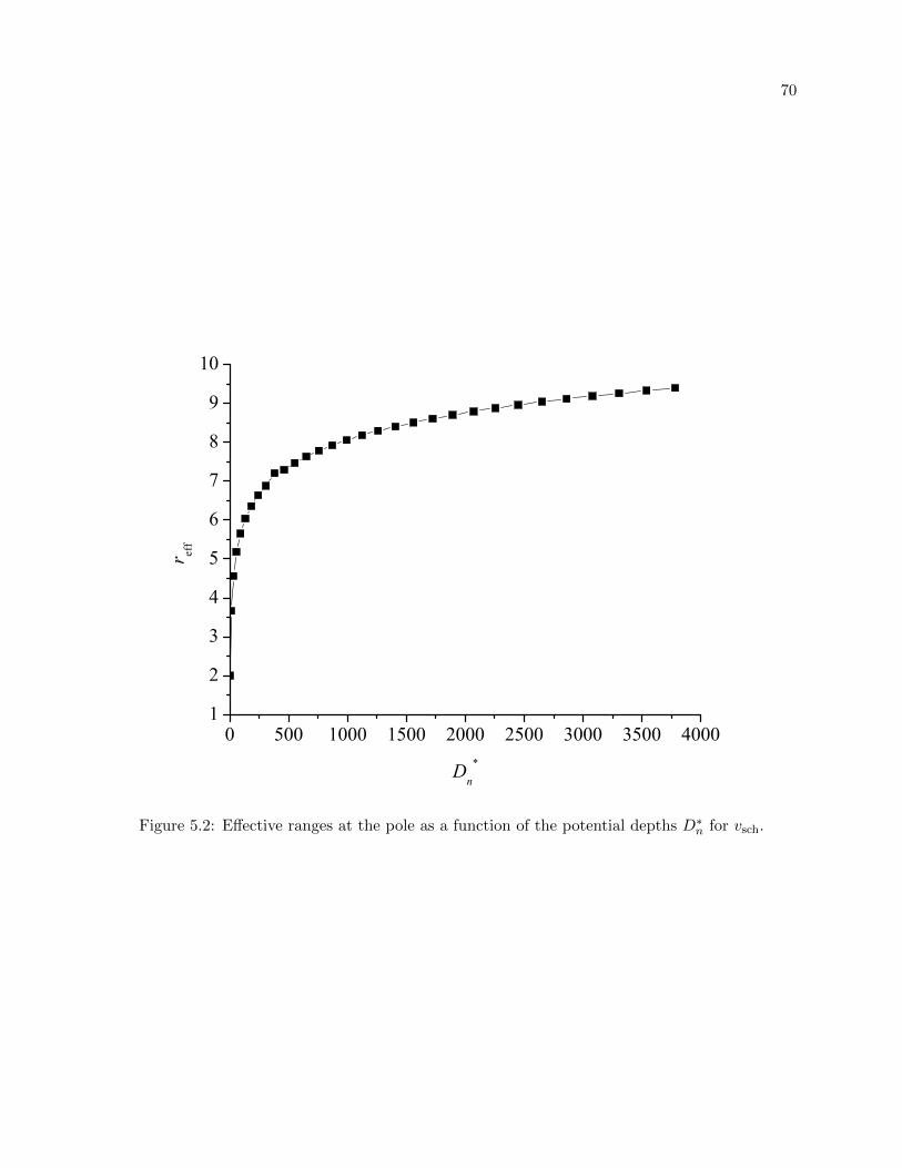
70

0 500 1000 1500 2000 2500 3000 3500 40001

2

3

4

5

6

7

8

9

10

r eff

Dn*

Figure 5.2: Effective ranges at the pole as a function of the potential depths D∗n for vsch.

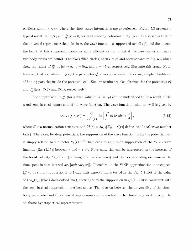
71

particles within r < r0, where the short-range interactions are experienced. Figure 5.3 presents a

typical result for |a|/r0 and ξinp (k → 0) for the two-body potential in Eq. (5.2). It also shows that in

the universal regime near the poles in a, the wave function is suppressed (small ξinp ) and documents

the fact that this suppression becomes more efficient as the potential becomes deeper and more

two-body states are bound. The black filled circles, open circles and open squares in Fig. 5.3 which

show the values of ξinp at |a| → ∞, a = 5r0, and a = −5r0, respectively, illustrate this trend. Note,

however, that for values |a| . r0, the parameter ξinp quickly increases, indicating a higher likelihood

of finding particles inside the potential well. Similar results are also obtained for the potentials vaλ

and vbλ [Eqs. (5.3) and (5.4), respectively].

The suppression in ξinp (for a fixed value of |a| r0) can be understood to be a result of the

usual semiclassical suppression of the wave function. The wave function inside the well is given by

ψWKB(r < r0) =C

k1/2L (r)

sin

[∫ r

kL(r′)dr′ +π

4

], (5.15)

where C is a normalization constant, and k2L(r) = 2µ2b[E2b − v(r)] defines the local wave number

kL(r). Therefore, for deep potentials, the suppression of the wave function inside the potential well

is simply related to the factor kL(r)−1/2 that leads to amplitude suppression of the WKB wave

function [Eq. (5.15)] between r and r + dr. Physically, this can be interpreted as the increase of

the local velocity ~kL(r)/m (m being the particle mass) and the corresponding decrease in the

time spent in that interval dr, [mdr/~kL(r)]. Therefore, in the WKB approximation, one expects

ξinp to be simply proportional to 1/kL. This expectation is tested in the Fig. 5.3 plot of the value

of 1/kL(r0) (black dash-dotted line), showing that the suppression in ξinp (k → 0) is consistent with

the semiclassical suppression described above. The relation between the universality of the three-

body parameter and this classical suppression can be studied in the three-body level through the

adiabatic hyperspherical representation.

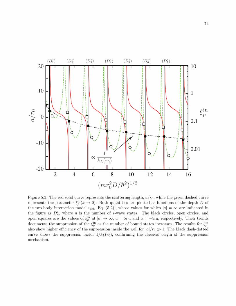
72

-20

-10

0

10

20

2 4 6 8 10 12 14 16

0.01

0.1

1

10

Figure 5.3: The red solid curve represents the scattering length, a/r0, while the green dashed curverepresents the parameter ξin

p (k → 0). Both quantities are plotted as functions of the depth D ofthe two-body interaction model vsch [Eq. (5.2)], whose values for which |a| = ∞ are indicated inthe figure as D∗n, where n is the number of s-wave states. The black circles, open circles, andopen squares are the values of ξin

p at |a| → ∞, a = 5r0, and a = −5r0, respectively. Their trends

documents the suppression of the ξinp as the number of bound states increases. The results for ξin

p

also show higher efficiency of the suppression inside the well for |a|/r0 1. The black dash-dottedcurve shows the suppression factor 1/kL(r0), confirming the classical origin of the suppressionmechanism.

73

5.3 Three-body adiabatic hyperspherical representation

Using the three-body potential as a summation of the two-body model potential from the last

section, Eq. (2.12) is solved for the adiabatic potential and channel functions. Treating problems

with deep two-body interactions — necessary to see strong inside-the-well suppression — requires us

to solve Eq. (2.12) for two-body model interactions that support many bound states, a challenge for

most theoretical approaches. Using our recently developed methodology in chapter 4 [95], however,

we were able to treat systems with up to 100 two-body rovibrational bound states.

Figure 5.4(a) shows the adiabatic potentials Uν at |a| = ∞ obtained using the two-body

Lennard-Jones potential supporting 25 dimer bound states. At first glance, it is difficult to identify

any universal properties of these potentials. Efimov physics, however, occurs at a very small

energy scale near the three-body breakup threshold. Indeed, a closer analysis of the energy range

|E| < ~2/mr2vdW [Fig. 5.4 (b)] reveals the universal properties of the key potential curve controlling

Efimov states and universal scattering properties.

Figure 5.4(b) shows one of our most important pieces of theoretical evidence for universality

of the three-body parameter: the effective adiabatic potentials Wν obtained using vaλ for more and

more two-body bound states converge to a single universal curve. [In some cases in Fig. 5.4 (b) we

have manually diabatized Wν near sharp avoided crossings in order to improve the visualization.

The details are discussed in Appendix E.] As one would expect, the usual Efimov behavior for the

effective potentials, Wν=−~2(s20 + 1/4)/2µ3bR

2 with s0 ≈ 1.00624, is recovered for R > 10rvdW. It

is remarkable, however, that Wν also converge to a universal potential for R < 10rvdW and, more

importantly, these effective potentials display a repulsive wall or barrier at R ≈ 2rvdW. This barrier

prevents the close collisions that would probe the short-range three-body physics, including three-

body forces known to be important in chemistry, thus making the three-body parameter universal,

as we will confirm below. This is in fact our most striking result: a sharp cliff or attraction

in the two-body interactions produces a strongly repulsive universal barrier in the

effective three-body interaction potential.

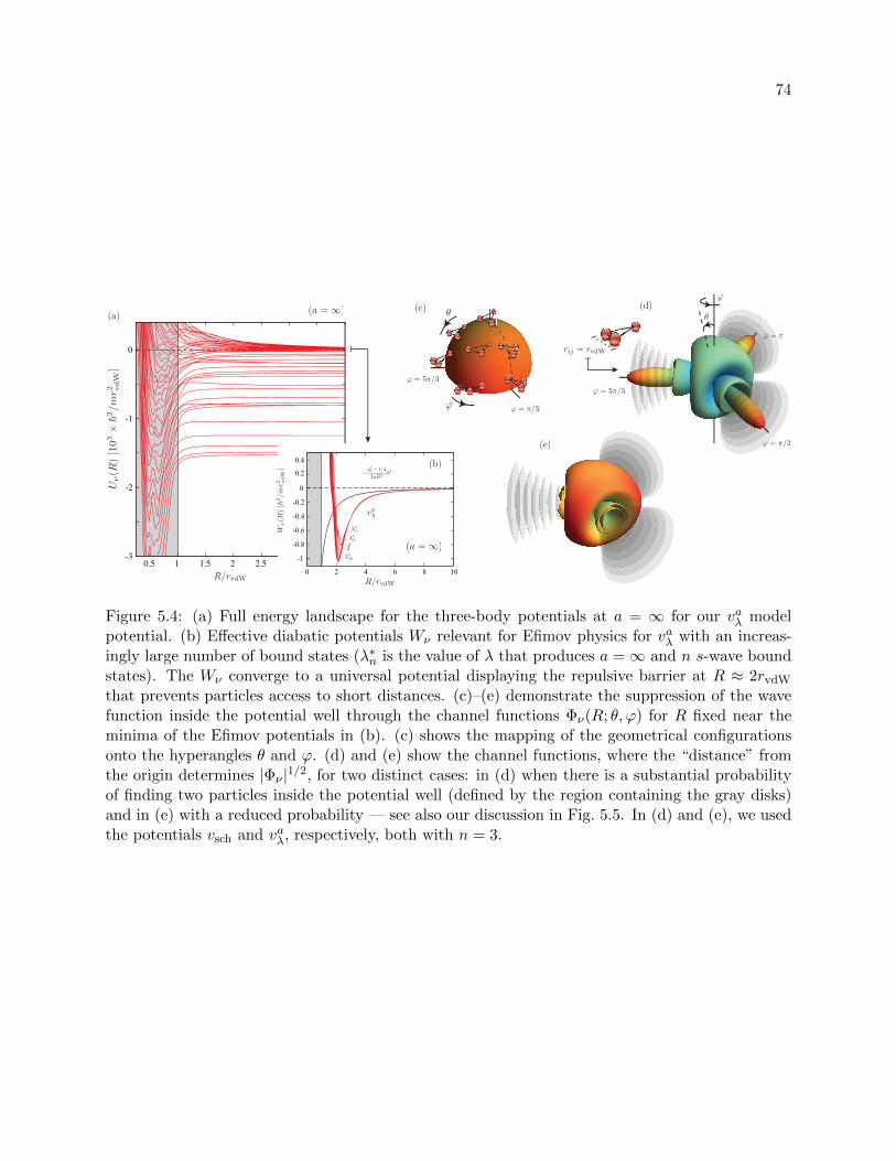
74

-3

-2

-1

0

0.5 1 1.5 2 2.5 3 3.5 4-1

-0.8

-0.6

-0.4

-0.2

0

0.2

0.4

0 2 4 6 8 10

...

Figure 5.4: (a) Full energy landscape for the three-body potentials at a = ∞ for our vaλ modelpotential. (b) Effective diabatic potentials Wν relevant for Efimov physics for vaλ with an increas-ingly large number of bound states (λ∗n is the value of λ that produces a =∞ and n s-wave boundstates). The Wν converge to a universal potential displaying the repulsive barrier at R ≈ 2rvdW

that prevents particles access to short distances. (c)–(e) demonstrate the suppression of the wavefunction inside the potential well through the channel functions Φν(R; θ, ϕ) for R fixed near theminima of the Efimov potentials in (b). (c) shows the mapping of the geometrical configurationsonto the hyperangles θ and ϕ. (d) and (e) show the channel functions, where the “distance” fromthe origin determines |Φν |1/2, for two distinct cases: in (d) when there is a substantial probabilityof finding two particles inside the potential well (defined by the region containing the gray disks)and in (e) with a reduced probability — see also our discussion in Fig. 5.5. In (d) and (e), we usedthe potentials vsch and vaλ, respectively, both with n = 3.

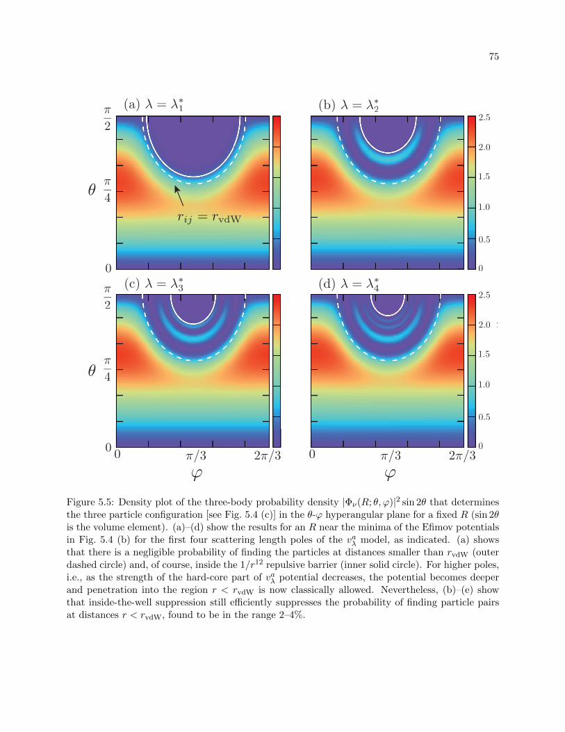
75

Figure 5.5: Density plot of the three-body probability density |Φν(R; θ, ϕ)|2 sin 2θ that determinesthe three particle configuration [see Fig. 5.4 (c)] in the θ-ϕ hyperangular plane for a fixed R (sin 2θis the volume element). (a)–(d) show the results for an R near the minima of the Efimov potentialsin Fig. 5.4 (b) for the first four scattering length poles of the vaλ model, as indicated. (a) showsthat there is a negligible probability of finding the particles at distances smaller than rvdW (outerdashed circle) and, of course, inside the 1/r12 repulsive barrier (inner solid circle). For higher poles,i.e., as the strength of the hard-core part of vaλ potential decreases, the potential becomes deeperand penetration into the region r < rvdW is now classically allowed. Nevertheless, (b)–(e) showthat inside-the-well suppression still efficiently suppresses the probability of finding particle pairsat distances r < rvdW, found to be in the range 2–4%.

76

Qualitatively, this universality derives from the reduced probability of finding particles inside

the attractive two-body potential well. This effect can be seen in terms of the channel functions

Φν , in Figs. 5.4 (c)–(d) and the hyperangular probability densities in Fig. 5.5. In the adiabatic

hyperspherical representation, the space forbidden to the particles fills an increasingly larger portion

of the hyperangular volume as R decreases. This evolution can be visualized as the dashed lines

in Fig. 5.5 (a)–(d) expanding outward. In the process, the channel function Φν is squeezed into an

increasingly smaller volume, driving its kinetic energy higher and producing the repulsive barrier in

the universal Efimov potential. Moreover, this suppression implies that the details of the interaction

should be largely unimportant. Consequently, different two-body model potentials should give

similar three-body potentials. Figure 5.6 demonstrates this universality by comparing Wν obtained

from different potential models supporting many bound states. Perhaps more importantly, it

compares them with the results obtained from a two-body model that replaces the deep well by a

hard wall, essentially eliminating the probability of observing any pair of atoms at short distances.

[See vhsvdW in Supplementary Eq. (5.5)]. Quantitatively, however, the fact that the barrier occurs

only at R ≈ 2rvdW indicates that universality might not be as robust as in the cases discussed in

Refs. [123, 124, 125, 126]. It is thus important to quantify the value of the three-body parameter

to assess the size of nonuniversal effects. The next section focuses on the numerical study of the

three-body parameter with different two-body model potentials and quantifies the universality.

In principle, the three-body parameter could be defined in terms of any observable related

to Efimov physics [104]. Two of its possible definitions are [104]: the value of a = a−3b < 0 at which

the first Efimov resonance appears in three-body recombination (see for instance Ref. [35]) and

κ∗ = (m|E03b|/~2)1/2, where E0

3b is the energy of the lowest Efimov state at |a| → ∞.

5.4 Three-body parameters

Strictly speaking, when there are two or more s-wave bound states in the two-body model,

the Efimov states are not real bound states but quasi-bound states with a finite width. This width

is related to the decay processes to deeper dimer channels (than the Efimov channel) because of

77

-1

-0.8

-0.6

-0.4

-0.2

0

0.2

0.4

0 2 4 6 8 10

Figure 5.6: The Efimov potential obtained from the different two-body potential models usedhere. The reasonably good agreement between the results obtained using models supporting manybound states (vsch, vaλ and vbλ) and vhs

vdW [obtained by replacing the deep potential well with ahard wall but having only one (zero-energy) bound state] supports our conclusion that the inside-the-well suppression of the wave function is the main physical mechanism behind the universalityof the three-body effective potentials. The differences between these potentials are seen to causedifferences of a few percent in the three-body parameter.

78

the couplings at short distances. It is well known that when there is a quasi-bound state buried

in the continua, the scattering amplitude in the continuous state and the quasi-bound state can

interfere with each other and form a Fano resonance. In our case, the scattering matrix elements

Sii for deeper atom-dimer thresholds (denoted by i’s) was calculated as a function of the energy E.

Near the resonance due to an Efimov state, the quantity |1− Sii|2 (which is closely related with

the elastic scattering cross section) is fitted with the formula

|1− Sii|2 = sa(q + ε)2

1 + ε2+ sb, (5.16)

where sa, sb, and q are fitting parameters, and ε =(E − E0

3b

)/(Γ0

3b/2)

gives the resonance position

(Efimov energy) E03b and the width Γ0

3b.

Figure 5.7 shows an example of fitting the resonance energy and the width using Fano line-

shapes. The system studied here consists of three identical bosons with a total angular momentum

of J = 0 interacting with each other via a Lennard-Jones potential vaλ. The λ is chosen to be equal

to λ∗2 corresponding to the case where the second s-wave bound state is exactly at the threshold.

There are three deeper dimer channels corresponding to a g-wave dimer, a d-wave dimer, and a

deep s-wave dimer. The calculated quantities |1− Sii|2 for each atom-dimer channel are shown

in the black squares, red triangles, and blue circles for the g-wave, d-wave and s-wave channel,

correspondingly. The solid curves are the results of the fitting formula in Eq. (5.16), and show a

very good agreement between the fitting and the numerical results. In this case, the Efimov energy

E03b ≈ −0.0498EvdW and Γ0

3b ≈ 0.0078EvdW are deduced from the fitting.

This method can also be applied to finding higher Efimov states and to finite scattering length

cases. Figure 5.8 shows the Efimov scenario using vbλ near the second pole λ = λ∗2. The red curve

with solid circles corresponds to the Efimov ground state, and the black curve with solid square

symbols represents the Efimov first-excited state. The blue dashed curve shows the shallowest

s-wave dimer energy. At the negative site, the Efimov energies cross the three-body break-up

threshold at some values of a−k , which can be deduced from extrapolations. For the case studied

here, a−0 ≈ −9.35 and a−1 ≈ −158.37 are deduced from extrapolations. The ratio a−1 /a−0 ≈ 16.93

79

-0.08 -0.07 -0.06 -0.05 -0.04 -0.03 -0.020.0

0.5

1.0

1.5

2.0

2.5

3.0

3.5

4.0

g

d

|1-S

ii|2

E /EvdW

s

Figure 5.7: Fitting the Efimov resonance using a fano lineshape [Eq. (5.16)] for a system using thetwo-body model potential vaλ with λ = λ∗2. The blue circles, red triangles, and black squares arethe numerically calculated |1 − Sii|2 for the three deeper atom-dimer channels (a g-wave dimer, ad-wave dimer, and a deeper s-wave dimer, correspondingly.) The curves are fitting results fromusing Eq. (5.16).

80

deviates from the universal value 22.7 because of the finite range correction. When an Efimov state

crosses the three-body break-up threshold, a resonance shows up in the three-body recombination

rate.

Figure 5.9 shows the three-body recombination rate as a function of scattering length and

exhibits a clear resonance structure. A zero-range model gives an analytical formula for the three-

body recombination rate near an Efimov resonance at zero temperature (E → 0) [104]:

K3 = AKsinh (2η)

sin2[s0 ln

(a/a−0

)]+ sinh2 η

. (5.17)

This formula is used to fit the numerically calculated three-body recombination rate and to deduce

the resonance position a−0 ≈ −9.18. This value is very close to the position of an Efimov state

crossing the threshold given by the extrapolation method mentioned in the last paragraph (which

is about -9.35). The small difference might be due to the finite range correction and the finite

temperature corrections.

Directly calculating K3 and extrapolating the Efimov energy can give approximately the

same answer for a−k . This fact has also been checked numerically for several other two-body model

potentials with 2–4 s-wave bound states. However, calculating the Efimov energy is usually faster

and more stable. Therefore, in the next subsection, the extrapolation method is used to study

a−3b ≡ a−0 for all the different two-body potential models.

5.4.1 Universality of the three-body parameter

To study the universality of the three-body parameter, different two-body potential models

are utilized. Our numerical results for κ∗ and a−3b are summarized in Figs. 5.10(a) and (b), respec-

tively, demonstrating their universality in the limit of many bound states. In fact, the values for

κ∗ and a−3b in this limit differ by no more than 15% from the vhsvdW results — κ∗ = 0.226(2)/rvdW

and a−3b = −9.73(3)rvdW [solid black line in Fig. 5.10(a) and (b)] — indicating, once again, that

the universality of the three-body parameter is dependent upon the suppression of the probability

density within the two-body potential wells. Given this picture, we attribute the variations of κ∗

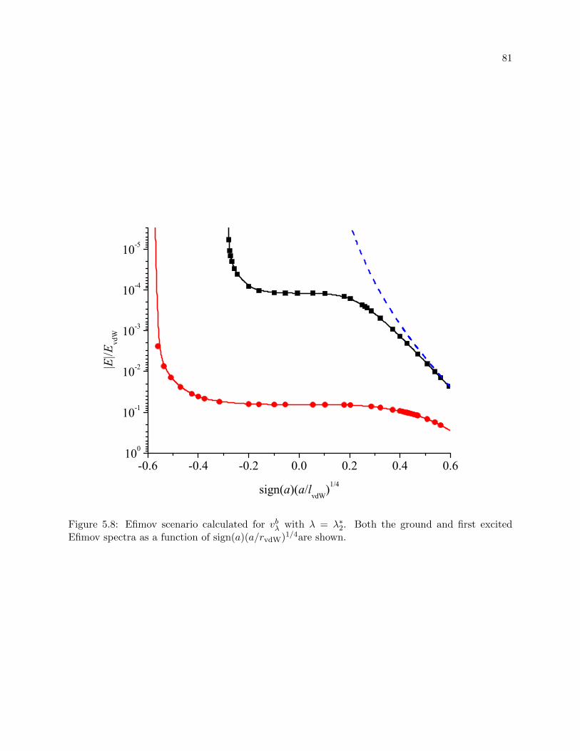
81

-0.6 -0.4 -0.2 0.0 0.2 0.4 0.6100

10-1

10-2

10-3

10-4

10-5

|E|/E

vdW

sign(a)(a/lvdW

)1/4

Figure 5.8: Efimov scenario calculated for vbλ with λ = λ∗2. Both the ground and first excitedEfimov spectra as a function of sign(a)(a/rvdW)1/4are shown.

82

4 8 12 16 201E-24

1E-23

1E-22

1E-21

1E-20

K3(c

m6 /s

)

|a|/rvdW

Figure 5.9: The Efimov resonance corresponding to the Efimov ground state. The black squaresare numerically calculated results, and the solid curve is the fitting result from using Eq. (5.17).

83

and a−3b in Fig. 5.10 to the small, but finite, probability of reaching short distances, thus introduc-

ing nonuniversal effects related to the details of the two- and three-body forces. Nevertheless, our

results for a−3b are consistent with the experimentally measured values for 133Cs [34, 6], 39K [7],

7Li [8, 9, 10], 6Li [11, 12, 13, 14],3 and 85Rb [15], all of which lie within about 15% of the vhsvdW

result. Curiously, if one simply averages the experimental values, then the result differs from the

vhsvdW result by less than 3%.

Previous treatments have failed to predict the universality of the three-body parameter for

various reasons. In treatments using zero-range interactions, for instance, the three-body param-

eter enters as a free parameter to cure the Thomas collapse [33], preventing any statement about

its universality. Finite-range models, such as those used in some of our own treatments [118] [cor-

responding to the results for vsch with n = 2 and 3 in Figs. 5.10 (a) and (b)], have failed for lack of

substantial suppression of the probability density in the two-body wells. This scenario, however,

should reflect better the situation for light nuclei having few bound states and shallow attraction.

In contrast to Ref. [118], other models [127, 128, 129, 125, 130, 131] have found better agreement

with experiment. Our analysis of these treatments, however, indicates that the two-body mod-

els used have many of the characteristics of our vhsvdW, therefore satisfying the prerequisite for a

universal three-body parameter.

A recent attempt [16] to explain the universality of the three-body parameter avoided ex-

plicit two-body models altogether, using instead an ad hoc hyperradial potential that bore little

resemblance to our numerical potentials in Fig. 5.4. This ad hoc three-body potential displayed

strong attraction at short distances in contrast to our key finding that a cliff of attraction for

two bodies produces a universal repulsive barrier in the three-body system. Consequently, even

though a universal three-body parameter was found in Ref. [16], the fundamental understanding

provided by the approach is uncertain. We also construct a simple single channel model according

to our numerical findings. The differences between the two models and our single channel model

3 For the experiments with 6Li [11, 12, 13, 14], we have determined a−3b by using the definition of the meanscattering length from: Wenz, A. N. et al., Phys. Rev. A 80, 040702(R) (2009).

84

0.1

0.2

0.3

0.4

0.5

0.6

0.7

1 2 3 4 5 6 7 8 9 10-14

-12

-10

-8

-6

-4

-2

0

1 2 3 4 5 6 7 8 9 10

0

0.1

0.2

0 5 10 15 20 25

Figure 5.10: Values for the three-body parameter (a) κ∗ and (b) a−3b as functions of the number nof two-body s-wave bound states for each of the potential model studied here. (c) Experimentalvalues for a−3b for 133Cs [6] (red: ×, +, , and ∗), 39K [7] (magenta: M), 7Li [8] (blue: •) and [9, 10](green: and ), 6Li [11, 12] (cyan: N and O) and [13, 14] (brown: H and ♦), and 85Rb [15] (black:). The gray region specifies a band where there is a ±15% deviation from the vhs

vdW results. Theinset of (a) shows the suppression parameter ξin

p [Eq. (5.11)] which can be roughly understood as

the degree of sensitivity to nonuniversal corrections. Since ξinp is always finite — even in the large

n limit — nonuniversal effects associated with the details of the short-range interactions can stillplay an important role. One example is the large deviation in κ∗ found for the vsch (n = 6) model,caused by a weakly bound g-wave state. For n > 10 we expect κ∗ and a−3b to lie within the rangeof 15% established for n ≤ 10.

85

are presented in detail in the next subsection.

5.4.2 Single channel approximation

The strong multichannel nature of the problem can be illustrated by comparing the results

obtained from a single channel approximation, i.e., Wνν′(R) = 0 (ν 6= ν ′), with our solutions of the

fully coupled system of equations. Figure 5.11 (a) shows the three-body parameter κ∗ [related to

the energy of the lowest Efimov state through the relation κ∗ = (mE/~2)1/2] obtained for the vaλ

model obtained in the single channel approximation (open triangles) as well as our full numerical

results (open circles). The disagreement between these quantities increases with the number of

s-wave bound states n, meaning that the physics controlling the results becomes more and more

multichannel in nature. Nevertheless, we find that by imposing a simple change in the adiabatic

potentials near the barrier — to make the barrier more repulsive [see Fig. 5.11 (b)] — the single

channel approximation for κ∗ [filled circles in Fig. 5.11 (a)] reproduces the full numerical calculations

much better. This agreement indicates that most of the nonadiabaticity of the problem is related to

the exact shape of the barrier and that, to some extent, the effect of the nonadiabatic couplings is

to make the effective potential Wν more repulsive. For these reasons and, of course, the universality

of our full calculations (see for instance Fig. 5.10), we believe that the short-range barrier in the

three-body effective potentials indeed offers a physically valid explanation of the universality of

the three-body parameter. We emphasize, though, that Fig. 4 only includes the results from our

essentially exact solutions of the full calculations. The single channel results discussed here are

intended only as support of our physical interpretation.

It is within this context that we analyzed the model proposed in Ref. [16]. In Ref. [16],

the three-body effective potential important for Efimov physics was estimated by considering the

different aspects controlling the physics at small and large distances. At distances comparable to

R = rvdW, it was assumed that the effective three-body potential is dominated by the contributions

from equilateral triangle geometries and included only on two-body interactions. Under these

assumptions, r12 = r23 = r31 = r giving R = 31/4r (note that our definition for R differs from that

86

0.18

0.2

0.22

0.24

0.26

0.28

0.3

0.32

1 2 3 4 5 6 7 8 9 10

-1

-0.5

0

0.5

1

1 2 3 4 5

Figure 5.11: (a) This figure compares the energies (as characterized by the three-body parameter κ∗)obtained from a single channel approximation with our full calculations. The three-body parameterκ∗ is shown for the vaλ model in the single channel approximation (open triangles) as well as forour full numerical results (open circles). The single channel approximation can be improved byimposing a simple change in the adiabatic potentials near the barrier, as is shown in (b). Therewe smoothly connect the potential for vaλ (red solid line) to the barrier obtained for vhsvdW (blacksolid line), resulting in the potential labeled by vaλ (green solid line). This new potential is actuallymore repulsive and has energies [filled circles in (a)] that are much closer to our full numericalcalculations.

87

used in Ref. [16]), the effective potential can be written as

Vm(R) = −C6/r612 − C6/r

623 − C6/r

631

= −3C6/r6 = −3× 33/2C6/R

6. (5.18)

This potential is expected to be valid for distances R < A = 4πΓ(1/4)−231/433/8rvdW ≈ 1.9rvdW

[120]. With our method, however, we have the means to check the validity of Eq. (5.18) by com-

paring it with our numerically calculated potentials. Figure 5.12 shows the three-body potentials

obtained using the vaλ(λ = λ∗10) model supporting a total of 100 two-body bound states. The

potential from Eq. (5.18) is the black solid line passing near the series of avoided crossings and

might be loosely viewed as diabatically connecting the fully numerical potentials. This relation is

reasonable given that this sequence of avoided crossings has been shown in Ref. [132] to be related

to the transition of the system from an equilateral triangle geometry to other geometries. This

figure therefore suggests that approximating the short range physics by Eq. (5.18) is not wholly

unphysical, but its validity depends on a strong assumption of diabaticity through a large number

of avoided crossings and is thus probably not an approximation satisfactory for a more quantitative

analysis.

The potential in Eq. (5.18), however, was not actually used in the calculations in Ref. [16].

Instead, it was used to motivate a claim that three-body quantum reflection plays an important

role, allowing the short range behavior to be replaced by a repulsive potential for distances R <

A ≈ 1.9rvdW. It is interesting to note that the value R ≈ 1.9rvdW obtained from Ref. [16] for the

position of the hard wall is quite close to the hyperradius where our potentials exhibit the universal

barrier (see Fig. E.1, for instance), indicating that A might have some physical meaning. It is worth

mentioning, however, that the barrier we observed in our calculations is model independent, i.e., it

doesn’t rely on the particular model used for the two-body interaction. For distances R > A, the

model in Ref. [16] assumed the three-body effective potentials to be given by the universal Efimov

formula,

VE(R) = −~2 s20 + 1/4

2µR2. (5.19)

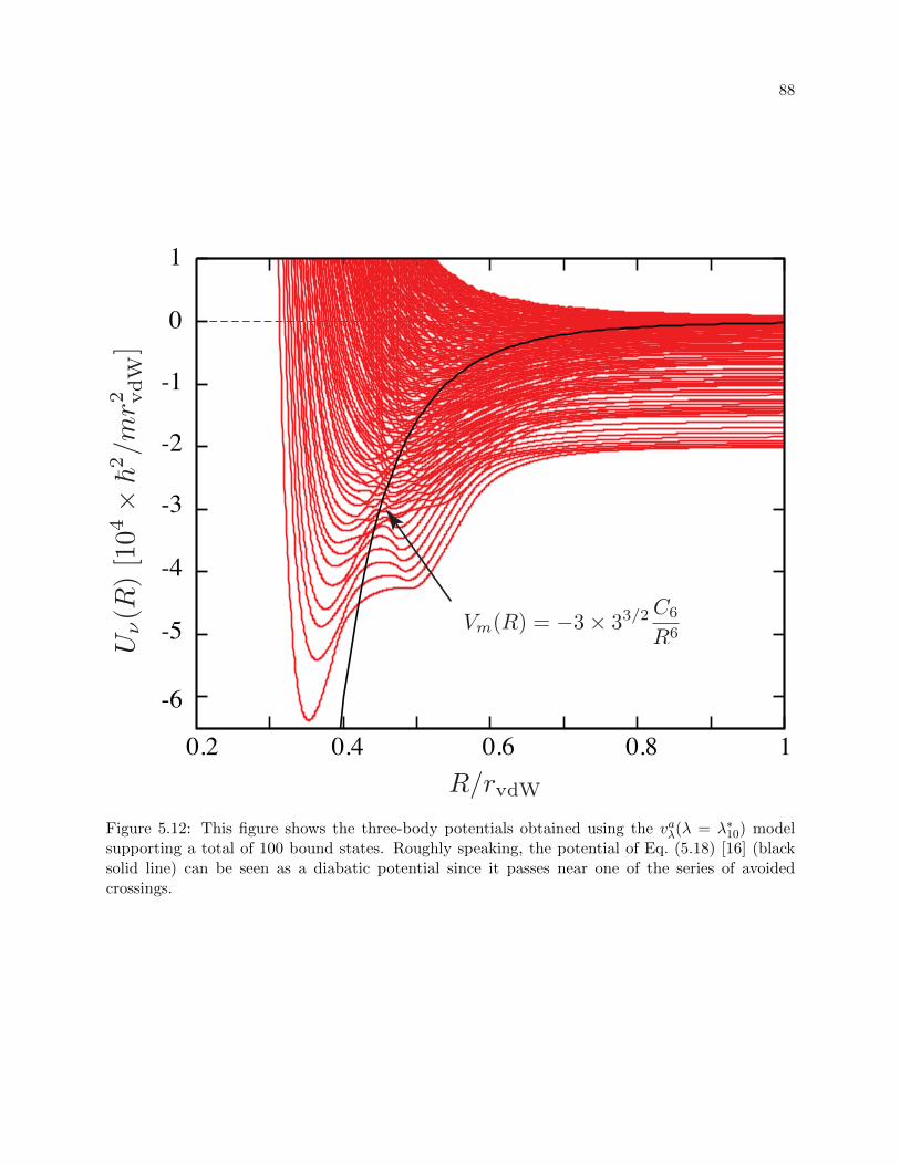
88

-6

-5

-4

-3

-2

-1

0

1

0.2 0.4 0.6 0.8 1

Figure 5.12: This figure shows the three-body potentials obtained using the vaλ(λ = λ∗10) modelsupporting a total of 100 bound states. Roughly speaking, the potential of Eq. (5.18) [16] (blacksolid line) can be seen as a diabatic potential since it passes near one of the series of avoidedcrossings.

89

It is well known [?], however, that this potential is valid for rvdW R |a|, and R = 1.9rvdW is

certainly out of this range. In fact, one can see in Fig. 1 (b) that the use of the Efimov potential

[Eq. (5.19)] for R < 10rvdW is a crude approximation. Nevertheless, using this model, Ref. [16]

obtains a−3b ≈ −9.48rvdW, a value consistent with experiments [34, 6, 7, 8, 9, 10, 11, 12, 13, 14, 15]

as well as with our present calculations for a−3b.

However, extending the model of Ref. [16] to the limit |a| =∞, we obtained κ∗ ≈ 0.037/rvdW.

Our result, by way of contrast, using vhsvdW [Eq. (5.5)] is κ∗ = 0.226(2)/rvdW. We also have tested the

effects of finite a corrections on the model of Ref. [16] by replacing Eq. (5.19) with the three-body

potential obtained with a zero-range model of the two-body interactions [133]. These corrections

are particularly important near R = |a|. With this modification, the model of Ref. [16] leads to

a−3b ≈ −39.96rvdW. For these reasons, we believe that this model’s agreement with our results and

experimental data is fortuitous.

While multichannel couplings are needed to quantitatively describe this system, it is possible

to construct an effective hyperradial potential curve that correctly describes the behavior of three

atoms in the universal regime. Such a potential curve could be useful for simplified future studies.

The approximate form obtained from the present study is:

2µr2vdW

~2W uν (R) ≈ − s2

0 + 1/4

(R/rvdW)2− 2.334

(R/rvdW)3− 1.348

(R/rvdW)4− 44.52

(R/rvdW)5+

4.0× 104

(R/rvdW)16. (5.20)

Here µ is the three-body reduced mass and rvdW is the two-body van der Waals length. For

comparison the speculative potential curve proposed by Chin [16] is shown, which does not resemble

the present result even qualitatively at small distances, as it exhibits far too little attraction in the

region R = 2− 5rvdW.

5.5 Summary

In summary, our theoretical examination shows that the three-body parameter controlling

much of universal Efimov physics can also be a universal parameter under certain circumstances

which should be realized in most ultracold neutral atom experiments. Provided the underlying

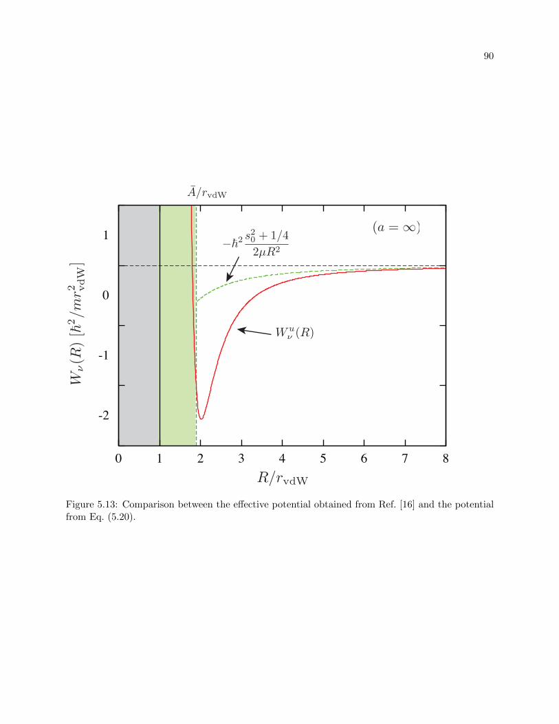
90

-2

-1

0

1

0 1 2 3 4 5 6 7 8

Figure 5.13: Comparison between the effective potential obtained from Ref. [16] and the potentialfrom Eq. (5.20).

91

two-body short-range interaction supports a large number of bound states, or it has some other

property leads to the suppression of the wave function at short distances, three-body properties

associated with Efimov physics can be expected to be universal. This surprising new scenario could

not have been, and was not, anticipated from the simple model calculations to date. Ironically,

increasing the complexity of the model simplified the outcome by effectively eliminating the impact

of the deeply bound two- and three-body states on the low-energy bound and scattering three-body

observables. That is, the three-body parameter becomes largely universal.

While these arguments suggest universality also for the three-body parameter in heteronuclear

systems that exhibit Efimov physics with only resonant interspecies two-body interactions, verifying

this prediction is a high priority for future theory and experiment.

Equally important is the exploration of the relationship between a < 0 and a > 0 Efimov

features — currently a subject of a number of controversies [6] — under the new perspective our

present work offers.

Chapter 6

Efimov physics on the positive side

In the previous chapter, Efimov resonances of three-body recombination rates K3 for a < 0

have been studied. The universal three-body parameter a−3b ≈ −9.73rvdW is found to be consistent

in recent experiments of ultracold atomic gases. Although through a very different mechanism,

Efimov physics also affects the three-body recombination rates on the positive side (a > 0), which

is the focus of this chapter. On the positive side, the three-body recombination rate shows a

series of minima on top of an a4 overall scaling. In principle, there are an infinite number of

these minima a+k that obey a universal relation a+

k+1/a+k ≈ 22.7 for three identical bosons, a

clear Efimov feature predicted by [102, 35]. The universality in the three-body parameter that

was discussed in the preceding chapter implies that the position of the first minimum a+0 (and

all other a+k ) should also be universal, and this is confirmed by the numerical studies reported

in the present chapter. The mechanism responsible for these minima is also studied. Reference

[35] discovered that the mechanism causing these minima is a quantum interference phenomenon

— the so called “Stuckelberg minima”. This mechanism is examined through an analysis of the

partial recombination rates in all the final channels. In addition, two universal enhancements in

three-body recombination are found around a ≈ 0.956 rvdW. These two enhancements are found to

be associated with a universal d-wave dimer, crossing the three-body threshold, for systems with

two-body van der Waals potentials .

In this chapter, the Lennard-Jones potential vaλ in Eq. (5.3) is adopted to study three-body

recombination rates on the positive side. The three-body recombination rates are calculated for

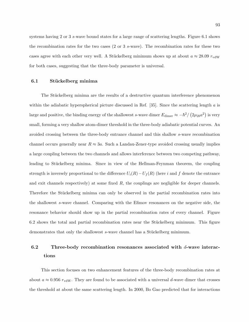
93

systems having 2 or 3 s-wave bound states for a large range of scattering lengths. Figure 6.1 shows

the recombination rates for the two cases (2 or 3 s-wave). The recombination rates for these two

cases agree with each other very well. A Stuckelberg minimum shows up at about a ≈ 28.09 rvdW

for both cases, suggesting that the three-body parameter is universal.

6.1 Stuckelberg minima

The Stuckelberg minima are the results of a destructive quantum interference phenomenon

within the adiabatic hyperspherical picture discussed in Ref. [35]. Since the scattering length a is

large and positive, the binding energy of the shallowest s-wave dimer Edimer ≈ −~2/(2µ2ba

2)

is very

small, forming a very shallow atom-dimer threshold in the three-body adiabatic potential curves. An

avoided crossing between the three-body entrance channel and this shallow s-wave recombination

channel occurs generally near R ≈ 3a. Such a Landau-Zener-type avoided crossing usually implies

a large coupling between the two channels and allows interference between two competing pathway,

leading to Stuckelberg minima. Since in view of the Hellman-Feynman theorem, the coupling

strength is inversely proportional to the difference Ui(R)−Uf (R) (here i and f denote the entrance

and exit channels respectively) at some fixed R, the couplings are negligible for deeper channels.

Therefore the Stuckelberg minima can only be observed in the partial recombination rates into

the shallowest s-wave channel. Comparing with the Efimov resonances on the negative side, the

resonance behavior should show up in the partial recombination rates of every channel. Figure

6.2 shows the total and partial recombination rates near the Stuckelberg minimum. This figure

demonstrates that only the shallowest s-wave channel has a Stuckelberg minimum.

6.2 Three-body recombination resonances associated with d-wave interac-

tions

This section focuses on two enhancement features of the three-body recombination rates at

about a ≈ 0.956 rvdW. They are found to be associated with a universal d-wave dimer that crosses

the threshold at about the same scattering length. In 2000, Bo Gao predicted that for interactions

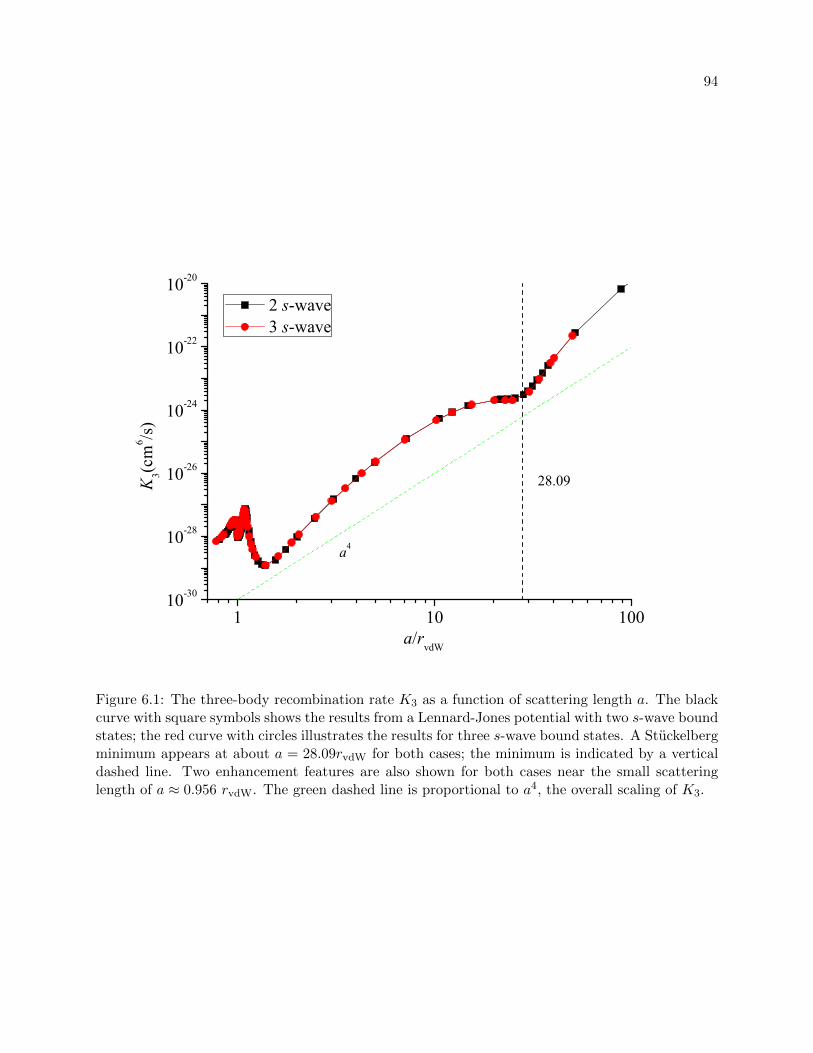
94

1 10 10010-30

10-28

10-26

10-24

10-22

10-20

a4

28.09K3(c

m6 /s

)

a/rvdW

2 s-wave 3 s-wave

Figure 6.1: The three-body recombination rate K3 as a function of scattering length a. The blackcurve with square symbols shows the results from a Lennard-Jones potential with two s-wave boundstates; the red curve with circles illustrates the results for three s-wave bound states. A Stuckelbergminimum appears at about a = 28.09rvdW for both cases; the minimum is indicated by a verticaldashed line. Two enhancement features are also shown for both cases near the small scatteringlength of a ≈ 0.956 rvdW. The green dashed line is proportional to a4, the overall scaling of K3.

95

20 40 60 80 1001E-27

1E-25

1E-23

1E-21

K3(c

m6 /s

)

a/rvdW

Figure 6.2: The total and partial three-body recombination rate K3 as a function of scatteringlength a. The black curve with square symbols shows the total recombination rate, and the redcurve with circle symbols shows the partial recombination rate for the shallowest s-wave dimerchannel. The other curves shows the partial recombination rate for deeper atom-dimer channels.The Stuckelberg minimum only shows up in the shallowest s-wave dimmer channel, but not thedeeper atom-dimer channels.

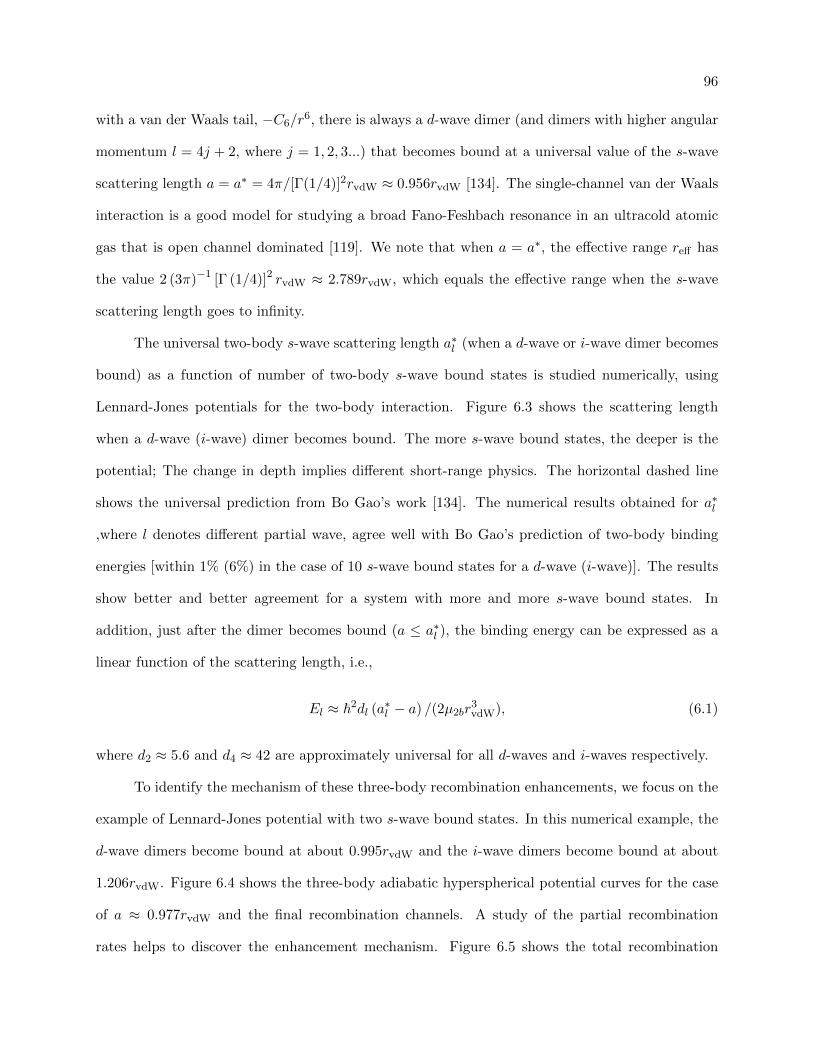
96

with a van der Waals tail, −C6/r6, there is always a d-wave dimer (and dimers with higher angular

momentum l = 4j + 2, where j = 1, 2, 3...) that becomes bound at a universal value of the s-wave

scattering length a = a∗ = 4π/[Γ(1/4)]2rvdW ≈ 0.956rvdW [134]. The single-channel van der Waals

interaction is a good model for studying a broad Fano-Feshbach resonance in an ultracold atomic

gas that is open channel dominated [119]. We note that when a = a∗, the effective range reff has

the value 2 (3π)−1 [Γ (1/4)]2 rvdW ≈ 2.789rvdW, which equals the effective range when the s-wave

scattering length goes to infinity.

The universal two-body s-wave scattering length a∗l (when a d-wave or i-wave dimer becomes

bound) as a function of number of two-body s-wave bound states is studied numerically, using

Lennard-Jones potentials for the two-body interaction. Figure 6.3 shows the scattering length

when a d-wave (i-wave) dimer becomes bound. The more s-wave bound states, the deeper is the

potential; The change in depth implies different short-range physics. The horizontal dashed line

shows the universal prediction from Bo Gao’s work [134]. The numerical results obtained for a∗l

,where l denotes different partial wave, agree well with Bo Gao’s prediction of two-body binding

energies [within 1% (6%) in the case of 10 s-wave bound states for a d-wave (i-wave)]. The results

show better and better agreement for a system with more and more s-wave bound states. In

addition, just after the dimer becomes bound (a ≤ a∗l ), the binding energy can be expressed as a

linear function of the scattering length, i.e.,

El ≈ ~2dl (a∗l − a) /(2µ2br

3vdW), (6.1)

where d2 ≈ 5.6 and d4 ≈ 42 are approximately universal for all d-waves and i-waves respectively.

To identify the mechanism of these three-body recombination enhancements, we focus on the

example of Lennard-Jones potential with two s-wave bound states. In this numerical example, the

d-wave dimers become bound at about 0.995rvdW and the i-wave dimers become bound at about

1.206rvdW. Figure 6.4 shows the three-body adiabatic hyperspherical potential curves for the case

of a ≈ 0.977rvdW and the final recombination channels. A study of the partial recombination

rates helps to discover the enhancement mechanism. Figure 6.5 shows the total recombination

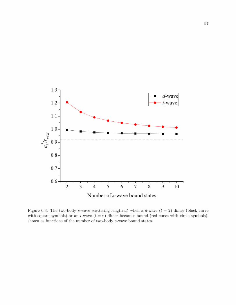
97

2 3 4 5 6 7 8 9 100.6

0.7

0.8

0.9

1.0

1.1

1.2

1.3

a l* /rvdW

Number of s-wave bound states

d-wave i-wave

Figure 6.3: The two-body s-wave scattering length a∗l when a d-wave (l = 2) dimer (black curvewith square symbols) or an i-wave (l = 6) dimer becomes bound (red curve with circle symbols),shown as functions of the number of two-body s-wave bound states.

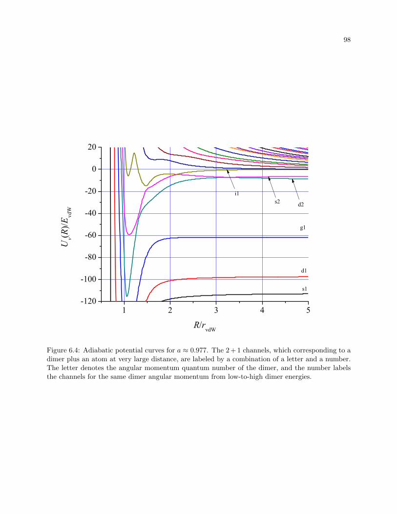
98

1 2 3 4 5-120

-100

-80

-60

-40

-20

0

20

s2 d2

i1

g1

d1

U(R)/E

vdW

R/rvdW

s1

Figure 6.4: Adiabatic potential curves for a ≈ 0.977. The 2 + 1 channels, which corresponding to adimer plus an atom at very large distance, are labeled by a combination of a letter and a number.The letter denotes the angular momentum quantum number of the dimer, and the number labelsthe channels for the same dimer angular momentum from low-to-high dimer energies.

99

rate (K3) and the partial recombination rates (Kf3 ) for every recombination channel f as functions

of the scattering length a, near the appearance of a new d-wave dimer threshold. The three-body

recombination rates show two enhancements with peaks A (aA ≈ 1.09rvdW) and B (aB ≈ 0.98rvdW).

An enhancement around the peak A appears in all the partial three-body recombination rates

right before the d-wave dimer becomes bound. After the d-wave becomes bound and forms a new

threshold, the K3 rate enhancement B is dominated by the partial rate in this new threshold, which

is indicated in the inset of Fig. 6.5. These features suggest that the peak A might be a resonance

due to that a three-body state crosses the three-body threshold, while the peak B seems to relate

to some threshold behavior. The behavior of the effective potential curves near these enhancements

gives qualitative insight into their origin.

Figure. 6.6 (I) shows the adiabatic hyperspherical potential curves at the resonance peak A.

Only the channels relevant to the resonances are shown in this figure. The red dashed-line shows

the effective hyperspherical potential. We have manually diabatized the potential near an avoid

crossing (see Appendix E) that doesn’t play an important role, and show it in the black solid curve.

The black solid curve shows an outer barrier, and a three-body state can be supported for this

potential. To check whether there is a three-body state near the threshold, a calculation of the

WKB phase at zero scattering energy is carried out:

φWKB =

∫ Rb

Ra

~√−2µ3bWνν (R)

dR, (6.2)

where Ra and Rb are the classical turning points shown in Fig. 6.6 (I). The calculated WKB phase

φWKB is about 0.51π, which is a strong evidence of the existence of a three-body state. It is this

three-body state associated with the d-wave dimer state crossing the three-body break-up threshold

that causes the three-body recombination resonances. The physical picture is that the three-body

state at threshold can cause the system to be within the short-range potential valley for a long time,

hence making it more likely that the system will decay into deeper channels. Figure. 6.6 (II) shows

the effective potential Wνν(R) as a function of R around the enhancement peak B. Three points

(a), (b), and (c) in the inset of Fig. 6.6 are chosen for the study of the Wνν corresponding to the

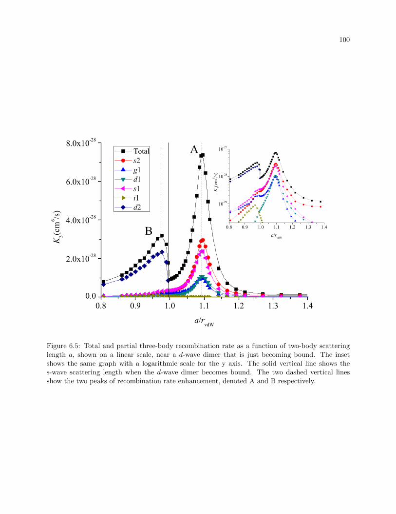
100

0.8 0.9 1.0 1.1 1.2 1.3 1.40.0

2.0x10-28

4.0x10-28

6.0x10-28

8.0x10-28

K3(c

m6 /s

)

B

K3(c

m6 /s

)

a/rvdW

Total s2 g1 d1 s1 i1 d2

A

0.8 0.9 1.0 1.1 1.2 1.3 1.4

10-29

10-28

10-27

a/rvdW

Figure 6.5: Total and partial three-body recombination rate as a function of two-body scatteringlength a, shown on a linear scale, near a d-wave dimer that is just becoming bound. The insetshows the same graph with a logarithmic scale for the y axis. The solid vertical line shows thes-wave scattering length when the d-wave dimer becomes bound. The two dashed vertical linesshow the two peaks of recombination rate enhancement, denoted A and B respectively.

101

solid curves, dashed curves, and dash-dotted curves. For each point, the thin curve is the entrance

channels that do not change much between the three points. The thick curve is the most important

recombination channel: the new d-wave channel. It is clear that from point (a) to (c), the barrier

and the threshold become lower and lower. When the maximum of the barrier is about to be lower

than the three-body threshold, three-body recombination starts decreasing. This decrease may be

due to the fact that when the maximum of the barrier is well above the three-body threshold, i.e.,

at point (a), the wave function of the exit channel has a large amplitude outside the barrier, and

has a large overlap with the entrance channel wave function. When the maximum of the barrier

becomes lower than the three-body break-up channel, i.e., at point (c), the wave function will have

large amplitude inside the three-body potential valley and have much less overlap with the entrance

channel wave function. The WKB phase calculated for these three-points is also not close to π/2

indicating that this enhancement is not due to a three-body state resonance. It is therefore not

shown in the partial recombination rate for channels other than the newly formed d-wave.

6.3 Three-body state associated with the d-wave dimmer

While the Efimov states can be viewed as three-body states associated with an s-wave dimer

near threshold, the new three-body state discovered in the previous section is a three-body state that

can be associated with a d-wave dimer. Because of the existence of deeper atom-dimer thresholds,

this three-body state is actually a quasi-bound state. Figure 6.7 shows the three-body quasi-bound

state energy as a function of the scattering length a (red dots), with the error bars showing the

widths of the quasi-bound states. The red line represents a fitting formula:

E3b/[~2/

(2µ2br

2vdW

)]= d3b (a∗3b − a) /rvdW + e3b (a∗3b − a)2 /r2

vdW, (6.3)

where a∗3b ≈ 1.09rvdW, d3b ≈ 8.21 and e3b ≈ 10.01. For comparison, the figure also shows the d-wave

energy as the black curve with solid square symbols. The three-body energy crosses the threshold

at a ≈ 1.09rvdW, which corresponds to peak A in K3. Comparing with the d-wave dimer energy

(the black curve with square symbols in Fig. 6.7), the three-body energy is shown to be always

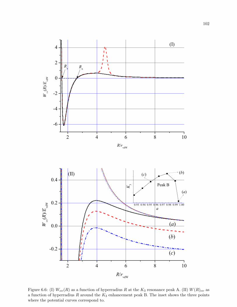
102

2 4 6 8 10

-6

-4

-2

0

2

4

Rb

W(R

)/Evd

W

R/rvdW

(I)

Ra

2 4 6 8 10

-0.2

0.0

0.2

0.4(II)

(c)

(b)

W(R)/E

vdW

R/rvdW

(a)

0.93 0.94 0.95 0.96 0.97 0.98 0.99 1.00

(c) (b)

K3

a

(a)

Peak B

Figure 6.6: (I) Wνν(R) as a function of hyperradius R at the K3 resonance peak A. (II) W (R)νν asa function of hyperradius R around the K3 enhancement peak B. The inset shows the three pointswhere the potential curves correspond to.

103

deeper than the dimer energy. The difference between the dimer and trimer energy also increases

when the scattering length becomes smaller, and the dimer becomes deeper. However, the width

of the three-body quasi-bound state does not seem to change appreciably.

From Gao’s analysis [134], it is known that there is also an i-wave dimer that becomes bound

at a nearby scattering length. However, the i-wave dimer does not affect these two peaks. The

i-wave channel has a very sharp avoided crossing with all the other channels. As a consequence,

the partial K3 rate is negligible as compared with the other partial rates. One explanation may

be that forming an i-wave (l = 6) dimer results in the exchange of a large amount of angular

momentum between the dimer and the additional atom. Therefore, although higher partial waves

l = 10, 14, 18... might also be formed at nearby scattering lengths, they are not expected to show

any strong features in the three-body recombination rate.

Finally, Fig. 6.8 compares the three-body enhancements for the model potential of Lennard-

Jones type, having either 2 or 3 s-wave bound states. The enhancement peaks of the two different

models differ by only 0.01 rvdW. This agrees with a small observed shift of the scattering length

where the d-wave dimer crosses the threshold. In this figure, the red (black) solid vertical line shows

where the d-wave dimer crosses the threshold for LJ with 2 (3) s-waves. The red (black) dashed

vertical line indicates where the three-body state associated with the d-wave cross the threshold for

LJ with 2 (3) s-waves. This result suggests that the three-body state associated with the d-wave

dimer is also universal.

6.4 Summary

In summary, we have calculated the three-body recombination rates for Lennard-Jones po-

tential with 2 and 3 s-wave bound states at the positive side. A universal Stuckelberg minimum for

the two cases is found at around a = 28.09 rvdW, and two universal enhancement peaks are found

at about a = 0.995 rvdW. In particular, one of the enhancement peaks is related with a universal

three-body state that is associated with a d-wave dimer.

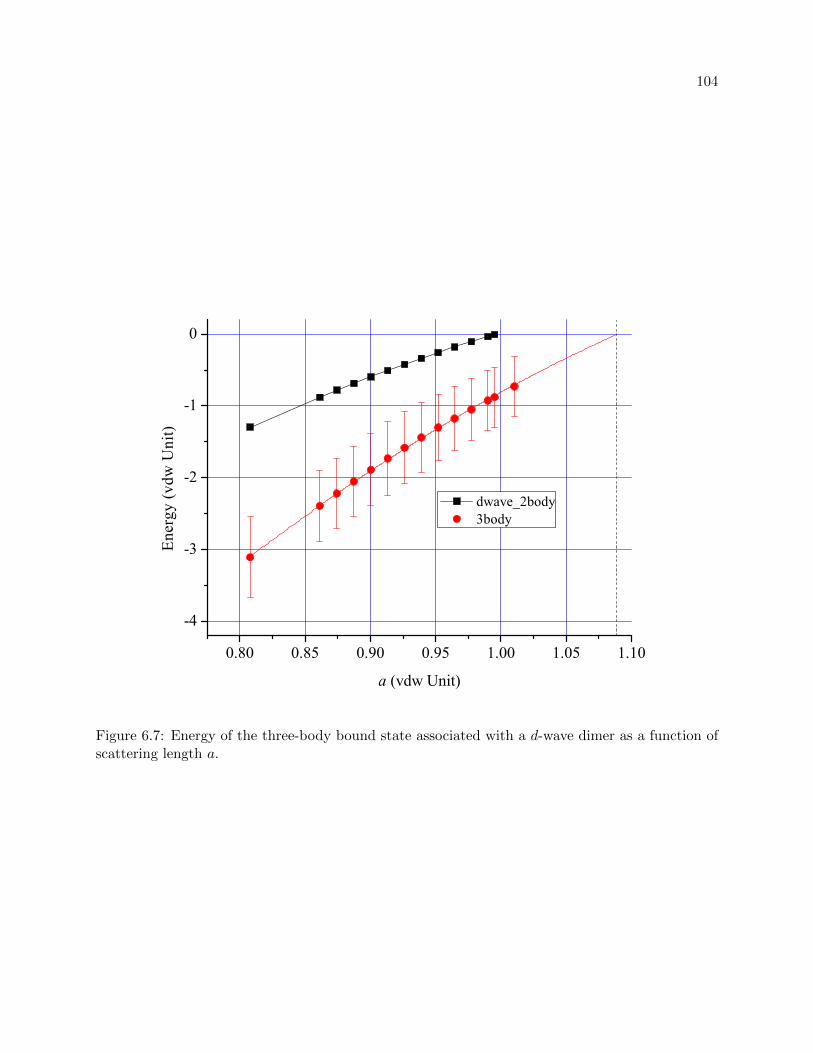
104

0.80 0.85 0.90 0.95 1.00 1.05 1.10

-4

-3

-2

-1

0

Ener

gy (v

dw U

nit)

a (vdw Unit)

dwave_2body 3body

Figure 6.7: Energy of the three-body bound state associated with a d-wave dimer as a function ofscattering length a.

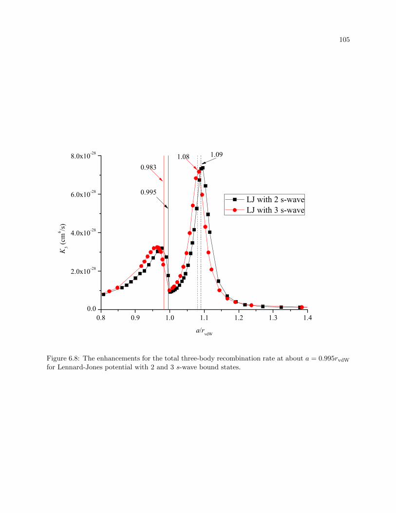
105

0.8 0.9 1.0 1.1 1.2 1.3 1.40.0

2.0x10-28

4.0x10-28

6.0x10-28

8.0x10-28

K3 (c

m6 /s

)

a/rvdW

LJ with 2 s-wave LJ with 3 s-wave

0.995

0.9831.08 1.09

Figure 6.8: The enhancements for the total three-body recombination rate at about a = 0.995rvdW

for Lennard-Jones potential with 2 and 3 s-wave bound states.

Bibliography

[1] C. M. Lindsay and B. J. McCall, J. Mol. Spectrosc. 210, 60 (2001).

[2] I. Dabrowski and G. Herzberg, Can. J. Phys. 58, 1238 (1980).

[3] G. Herzberg and J. K. G. Watson, Can. J. Phys. 58, 1250 (1980).

[4] G. Herzberg, H. Lew, J. J. Sloan, and J. K. G. Watson, Can. J. Phys. 59, 428 (1981).

[5] G. Herzberg, J. T. Hougen, and J. K. G. Watson, Can. J. Phys. 60, 1261 (1982).

[6] C. Chin, R. Grimm, P. S. Julienne, and E. Tiesinga, Rev. Mod. Phys. 82, 1225 (2010).

[7] M. Zaccanti, B. Deissler, C. D’Errico, M. Fattori, M. Jona-Lasinio, S. Muller, G. Roati,M. Inguscio, and G. Modugno, Phys. Rev. C 66, 064001 (2002).

[8] S. E. Pollack, D. Dries, and R. G. Hulet, Science 326, 1683 (2009).

[9] N. Gross, Z. Shotan, S. Kokkelmans, and L. Khaykovich, Phys. Rev. Lett. 103, 163202(2009).

[10] N. Gross, Z. Shotan, S. Kokkelmans, and L. Khaykovich, Phys. Rev. Lett. 105, 103203(2010).

[11] T. B. Ottenstein, T. Lompe, M. Kohnen, A. N. Wenz, and S. Jochim, Phys. Rev. Lett. 101,203202 (2008).

[12] T. Lompe, T. B. Ottenstein, F. Serwane, K. Viering, A. N. Wenz, G. Zurn, and S. Jochim,Phys. Rev. Lett. 105, 103201 (2010).

[13] J. H. Huckans, J. R. Williams, E. L. Hazlett, R. W. Stites, and K. M. O’Hara, Phys. Rev.Lett. 102, 165302 (2009).

[14] J. R. Williams, E. L. Hazlett, J. H. Huckans, R. W. Stites, Y. Zhang, and K. M. O’Hara,Phys. Rev. Lett. 103, 130404 (2009).

[15] J. R. Wild, P. Makotyn, J. M. Pino, E. A. Cornell, and D. S. Jin, Phys. Rev. Lett. 108,145305 (2012).

[16] C. Chin, arxiv: , 1111.1484 (2011).

[17] I. Newton, Philosophiæ Naturalis Principia Mathematica, 1687.

107

[18] E. W. Brown, An Introductory Treatise on the Lunar Theory, Cambridge Universit Press,1896.

[19] F. Haake, Quantum Signatures of Chaos, Edition: 2, Springer, 2001.

[20] K. Huang, C. N. Yang, and J. M. Luttinger, Phys. Rev. 105, 776 (1957).

[21] M. H. Anderson, J. R. Ensher, M. R. Matthews, C. E. Wieman, and E. A. Cornell, Science269, 198 (1995).

[22] C. C. Bradley, C. A. Sacket, J. J. Tollett, and R. G. Hulet, Phys. Rev. Lett. 75, 1687 (1995).

[23] K. B. Davis, M. R. Andrews, N. J. van Druten, D. S. Durfee, D. M. Kurn, and W. Ketterle,Phys. Rev. Lett. 75, 3969 (1995).

[24] L. M. Delves, Nucl. Phys. 9, 391 (1985).

[25] L. M. Delves, Nucl. Phys. 20, 275 (1960).

[26] V. Efimov, Sov. J. Nucl. Phys. 12, 589 (1971).

[27] J. Macek, J. Phys. B 1, 831 (1968).

[28] U. Fano, Phys. Today 29, 32 (1976).

[29] U. Fano, Rep. Prog. Phys. 46, 97 (1983).

[30] C. W. Clark and C. H. Greene, Phys. Rev. A 21, 1786 (1980).

[31] V. Kokoouline and C. H. Greene, Phys. Rev. A 68, 012703 (2003).

[32] N. P. Mehta, S. T. Rittenhouse, J. P. D’Incao, J. von Stecher, and C. H. Greene, Phys. Rev.Lett. 103, 153201 (2009).

[33] L. H. Thomas, Phys. Rev. 47, 903 (1935).

[34] T. Kraemer, M. Mark, P. Waldburger, J. G. Danzl, C. Chin, B. Engeser, A. D. Lange,K. Pilch, A. Jaakkola, H.-C. Nagerl, and R. Grimm, Nature 440, 315 (2006).

[35] B. D. Esry, C. H. Greene, and J. P. Burke, Phys. Rev. Lett. 83, 1751 (1999).

[36] B. D. Esry and C. H. Greene, Nature 440, 289 (2006).

[37] E. Herbst and W. Klemperer, Astrophys. J. 185, 505 (1973).

[38] W. D. Watson, Astrophys. J. 183, L17 (1973).

[39] L. Trafton, D. F. Lester, and K. L. Thompson, Astrophys. J. 343, L73 (1989).

[40] J. E. P. Connerney, R. Baron, T. Satoh, and T. Owen, Science 262, 1035 (1993).

[41] J. J. Thomson, Philos. Mag. 21, 225 (1911).

[42] T. Oka, Phys. Rev. Lett. 45, 531 (1980).

108

[43] B. J. McCall, A. J. Huneycutt, R. J. Saykally, T. R. Geballe, N. Djuric, G. H. Dunn, J. Sema-niak, O. Novotny, A. Al-Khalili, A. Ehlerding, F. Hellberg, S. Kalhori, A. Neau, R. Thomas,F. Osterdahl, and M. Larsson, Nature 422, 500 (2003).

[44] A. J. Huneycutt, Studies of Atmospheric and Interstellar Molecules Using Cavity RingdownSpectroscopy, PhD thesis, University of California, Berkeley, 2003.

[45] R. J. Saykally, E. A. Michael, J. Wang, and C. H. Greene, J. Chem. Phys. 133, 234302(2010).

[46] J. G. Frey and B. J. Howard, Chem. Phys. 99, 415 (1985).

[47] H. Suno, B. D. Esry, C. H. Greene, and J. P. Burke, Phys. Rev. A 65, 042725 (2002).

[48] R. C. Whitten and F. T. Smith, J. Math. Phys. 9, 1103 (1968).

[49] B. R. Johnson, J. Chem. Phys. 73, 5051 (1980).

[50] B. Lepetit, Z. Peng, , and A. Kuppermann, Chem. Phys. Lett. 166, 572 (1990).

[51] B. K. Kendrick, R. T. Pack, R. B. Walker, and E. F. Hayes, J. Chem. Phys. 110, 6673 (1999).

[52] B. K. Kendrick, R. T. Pack, R. B. Walker, and E. F. Hayes, J. Chem. Phys. 110, 6673 (1999).

[53] M. Aymar, C. H. Greene, and E. Luc-Koenig, Rev. Mod. Phys. 68, 1015 (1996).

[54] J. P. Burke, Theoretical investigation of cold alkali atom collisions, PhD thesis, Universityof Colorado at Boulder, 1999.

[55] E. Nielsen, D. V. Fedorov, A. S. Jensen, and E. Garrido, Phys. Rep. 347, 373 (2001).

[56] R. B. Nelson, AIAA Journal 14, 1201 (1976).

[57] E. Anderson, Z. Bai, C. Bischof, J. Demmel, J. Dongarra, J. D. Cros, A. Greenbaum, S. Ham-merling, A. Mckenney, S. Ostouchov, and D. Sorensen, LAPACK Users Guide, SIAM, 1992.

[58] U. Naumanm and O. Schenk, Combniatorial Scientific Computing, Champman and Hall,2012.

[59] J. V. Lill, G. A. Parker, and J. C. Light, Chem. Phys. Lett. 89, 483 (1982).

[60] T. N. Rescigno and C. W. McCurdy, Phys. Rev. A 62, 032706 (2000).

[61] D. E. Manolopoulos and R. E. Wyatt, Chem. Phys. Lett. 152, 23 (1998).

[62] K. L. Baluja and P. G. Burke, Comp. Phys. Comm. 27, 299 (1982).

[63] J. Wang and C. H. Greene, Phys. Rev. A 82, 022506 (2010).

[64] H. Helm, Phys. Rev. Lett. 56, 42 (1986).

[65] H. Helm, Phys. Rev. A 38, 3425 (1988).

[66] A. E. Orel, I. F. Schneider, and A. Suzor-Weiner, Philos. Trans. R. Soc. London, Ser. A 385,2445 (2000).

109

[67] V. Kokoouline, C. Greene, and B. Esry, Nature (London) 412, 891 (2001).

[68] C. Jungen and S. T. Pratt, Phys. Rev. Lett. 102, 023201 (2009).

[69] M. Vervloet and J. K. G. Watson, J. Mol. Spectrosc. 217, 255 (2003).

[70] M. J. Seaton, Rep. Prog. Phys. 46, 167 (1983).

[71] C. H. Greene and C. Jungen, Adv. At. Mol. Phys. 21, 51 (1985).

[72] H. Takagi, J. Phys. B 26, 4815 (1993).

[73] O. Motapon, F. O. W. Tamo, X. Urbain, and I. F. Schneider, Phys. Rev. A 77, 052711(2008).

[74] A. Giusti, J. Phys. B 13, 386 (1980).

[75] O. I. Tolstikhin, S. Watanabe, and M. Matsuzawa, J. Phys. B: At. Mol. Opt. Phys. 29, L389(1996).

[76] S. F. Santos, V. Kokoouline, and C. H. Greene, J. Chem. Phys. 127, 124309 (2007).

[77] W. Cencek, J. Rychlewski, R. Jaquet, and W. Kutzelnigg, J. Chem. Phys. 108, 2831 (1998).

[78] R. Jaquet, W. Cencek, W. Kutzelnigg, and J. Rychlewski, J. Chem. Phys. 108, 2837 (1998).

[79] M. Pavanello, L. Adamowicz, A. Alijah, N. F. Zobov, I. I. Mizus, O. L. Polyansky, J. Ten-nyson, T. Szidarovszky, A. G. Csaszar, M. Berg, A. Petrignani, and A. Wolf, Phys. Rev.Lett. 108, 023002 (2012).

[80] I. Mistrık, R. Reichle, U. Muller, H. Helm, M. Jungen, and J. A. Stephens, Phys. Rev. A 61,033410 (2000).

[81] A. Staib and W. Domcke, Z. Phys. D: At., Mol. Clusters 16, 275 (1990).

[82] E. E. Eyler and F. M. Pipkin, Phys. Rev. A 27, 2462 (1983).

[83] G. Herzberg and C. Jungen, J. Chem. Phys. 77, 5876 (1982).

[84] C. Jungen, I. Dabrowski, G. Herzberg, and D. J. W. Kendall, J. Chem. Phys. 91, 3926(1989).

[85] N. R. Badnell and M. J. Seaton, J. Phys. B. 32, 3955 (1999).

[86] J. D. Augspurger and C. E. Dykstra, J. Chem. Phys. 88, 3817 (1988).

[87] J. D. Augspurger and C. E. Dykstra, J. Chem. Phys. 91, 1384 (1989).

[88] A. Fridman, Plasma Chemistry, Cambridge University Press, Cambridge, 2008.

[89] J. Glosık, O. Novotny, A. Pysanenko, P. Zakouril, R. Plasil, P. Kudrna, and V. Poterya,Plasma Sources Sci. Technol. 12, S117 (2003).

[90] V. Kokoouline and C. H. Greene, Phys. Rev. A 69, 032711 (2004).

110

[91] J. A. Stephens and C. H. Greene, J. Chem. Phys. 102, 1579 (1995).

[92] G. Herzberg, Annu. Rev. Phys. Chem. 38, 27 (1987).

[93] J. Glosık, I. Korolov, R. Plasil, O. Novotny, T. Kotrik, P. Hlavenka, J. Varju, I. A. Mikhailov,V. Kokoouline, and C. H. Greene, J. Phys. B – At. Mol. Opt. 41, 191001 (2008).

[94] D. R. Bates and S. P. Khare, Proc. Phys. Soc. , 231 (1965).

[95] J. Wang, J. P. D’Incao, and C. H. Greene, Phys. Rev. A 84, 052721 (2011).

[96] J. Cubizolles, S. J. J. M. F. K. T. Bourdel, G. V. Shlyapnikov, and C. Salomon, Phys. Rev.Lett. 91, 240401 (2003).

[97] S. Jochim, M. Bartenstein, A. Altmeyer, G. Hendl, C. Chin, J. H. Denschlag, and R. Grimm,Phys. Rev. Lett. 91, 240402 (2003).

[98] M. W. Zwierlein, C. A. Stan, C. H. Schunck, S. M. F. Raupach, Z. H. S. Gupta, and W. Ket-terle, Phys. Rev. Lett. 91, 250401 (2003).

[99] J. P. D’Incao and B. D. Esry, Phys. Rev. Lett. 100, 163201 (2008).

[100] B. Borca, J. W. Dunn, V. Kokoouline, and C. H. Greene, Phys. Rev. Lett. 91, 070404 (2003).

[101] T. Weber, J. Herbig, and H.-C. N. M. Mark, Phys. Rev. Lett. 91, 123201 (2003).

[102] E. Nielsen and J. H. Macek, Phys. Rev. Lett. 83, 1566 (1999).

[103] J. P. D’Incao and B. D. Esry, Phys. Rev. Lett. 94, 213201 (2005).

[104] E. Braaten and H.-W. Hammer, Phys. Rep. 428, 259 (2006).

[105] J. P. D’Incao and B. D. Esry, Phys. Rev. Lett. 103, 083202 (2009).

[106] F. Ferlaino and R. Grimm, Physics 3, 9 (2010).

[107] H. Suno and B. D. Esry, Phys. Rev. A 78, 062701 (2008).

[108] H. Suno and B. D. Esry, Phys. Rev. A 80, 062702 (2009).

[109] Y. Wang, J. P. D’Incao, and B. D. Esry, Phys. Rev. A 83, 032703 (2011).

[110] H. Suno, J. Chem. Phys. 134, 064318 (2011).

[111] G. A. Parker, R. B. Walker, B. K. Kendrick, and R. T. Pack, J. Chem. Phys. 117, 6083(2002).

[112] F. D. Colavecchia, F. Mrugala, G. A. Parker, and R. T. Pack, J. Chem. Phys. 118, 10387(2003).

[113] B. D. Esry, C. H. Greene, and H. Suno, Phys. Rev. A 65, 010705 (2001).

[114] E. B. S. G. C. Maitland, M. Rigby and W. A. Wakeham, Intermolecular Forces, ClarendonPress, Oxford, 1981.

111

[115] J. Wang, J. P. D’Incao, B. D. Esry, and C. H. Greene, Phys. Rev. Lett. 108, 263001 (2012).

[116] P. Soldan, M. T. Cvitas, and J. M. Hutson, Phys. Rev. A 67, 054702 (2003).

[117] E. Epelbaum, A. Nogga, W. Glockle, H. Kamada, U.-G. Meißner, and H. Wita la, Phys. Rev.C 66, 064001 (2002).

[118] J. P. D’Incao, C. H. Greene, , and B. D. Esry, J. Phys. B 42, 044016 (2009).

[119] C. Chin, R. Grimm, P. S. Julienne, and E. Tiesinga, Rev. Mod. Phys. 82, 1225 (2010).

[120] V. V. Flambaum, G. F. Gribakin, and C. Harabati, Phys. Rev. A 59, 1998 (1993).

[121] G. F. Gribakin and V. V. Flambaum, Phys. Rev. A 48, 546 (1993).

[122] R. Cote, H. Friedrich, and J. Trost, Phys. Rev. A 56, 1781 (1997).

[123] Y. Wang, J. P. D’Incao, , and C. H. Greene, Phys. Rev. Lett. 106, 233201 (2011).

[124] D. S. Petrov, Phys. Rev. Lett. 93, 143201 (2004).

[125] P. Massignan and H. T. C. Stoof, Phys. Rev. Lett. 93, 143201 (2004).

[126] Y. Wang, J. P. D’Incao, , and B. D. Esry, Phys. Rev. A 83, 042710 (2011).

[127] P. Naidon and M. Ueda, Comptes Rendus Physique 12, 13 (2011).

[128] P. Naidon, E. Hiyama, and M. Ueda, arxiv , 1109.5807.

[129] S. Nakajima, M. Horikoshi, T. Mukaiyama, P. Naidon, and M. Ueda, Phys. Rev. Lett. 106,143201 (2011).

[130] M. D. Lee, T. Kohler, and P. S. Julienne, Phys. Rev. A 76, 012720 (2007).

[131] M. Jona-Lasinio and L. Pricoupenko, Phys. Rev. Lett. 104, 023201 (2010).

[132] D. Blume, C. H. Greene, and B. D. Esry, J. Chem. Phys. 113, 2145 (2000).

[133] S. T. Rittenhouse, N. P. Mehta, and C. H. Greene, Phys. Rev. A 82, 022706 (2010).

[134] B. Gao, Phys. Rev. A 62, 050702(R) (2000).

[135] D. A. Varshalovich, A. N. Moskalev, and V. K. Khersonskii, Quantum Theory of AngularMomentum, World Scientific, singapore, 1988.

[136] H. C. Longuet-Higgins, Advances in Spectroscopy, Interscience, New York, 1961.

[137] N. Gemelke, C.-L. Hung, X. Zhang, and C. Chin, arxiv: , 0812.1317 (2008).

Appendix A

Symmetry of R-matrix

The R-matrix R is a real and symmetric matrix. This symmetry is determined by the

properties of the radial Schrodinger equation [Eq. (2.17)], which can be rewritten as

d2

dR2F =

[2µ3b

~2(U − E1)−Q

]F − 2P

d

dRF, (A.1)

where 1 denotes an identity matrix. Inserting the expansion of the wave function [Eq. (2.16)] into

Eq. (2.20) gives

F =d

dRF + P × F . (A.2)

The definition of the R-matrix can then expressed as,

R(d

dRF + P × F

)= F . (A.3)

Taking derivatives of both sides of this equation leads to(d

dRR)(

d

dRF + P × F

)+R

[d2

dR2F +

(d

dRP

)F + P

(d

dRF

)]=

d

dRF . (A.4)

Replacing the second derivative of F by Eq. (A.1) gives us(d

dRR)(

d

dRF + P × F

)+R

[2µ3b

~2(U − E1)− P 2

]F = (R× P + 1)

d

dRF , (A.5)

with the help of the relation ddRP = −P 2 + Q. Finally, after multiplying both sides of Eq. (A.5)

with[(

ddRF + P × F

)]−1and using the definition of the R-matrix Eq. (A.3), we arrive at

d

dRR = −R

[2µ3b

~2(U − E1)− P 2

]R+ (R× P + 1)

(d

dRF

)(d

dRF + P × F

)−1

= −R[

2µ3b

~2(U − E1)− P 2

]R+ (R× P + 1) (1− P ×R) . (A.6)

113

Since P is antisymmetric and P 2 is symmetric, this equation implies that the symmetry of the

matrix R at one value of R immediately guarantees symmetry at all R values. In most problems,

the matrix R is diagonal in some region of space, often at small distances (R→ 0), which is enough

to prove that it will remain real and symmetric at all hyperradii.

The symmetry of R guarantees the symmetry of the reaction matrix K and the unity of

scattering matrix S. In the asymptomatic region at large hyperradii, the P matrix vanishes. The

relation between R and K is given by,

R[f ′ − g′K

]=[f − gK

](A.7)

or equivalently by [f ′ − g′K

]= R−1

[f − gK

]. (A.8)

Transposing on both sides of Eq.(A.7) gives

[f −KT g

]=[f ′ −KT g′

]R. (A.9)

Together, Eqs. (A.8) and Eq. (A.9) give the followings

[f −KT g

] [f ′ − g′K

]=[f ′ −KT g′

] [f − gK

], (A.10)

which can be transformed into

KT(dg

dRf − g

df

dR

)=

(gdf

dR−dg

dRf

)K. (A.11)

Since f and g are linearly independent solutions of the Schrodinger equation, their Wronskian has

the good property of

dg

dRf − g

df

dR= f

dg

dR−df

dRg =

2µ3b

~π1, (A.12)

whoich guarantees that KT = K. Therefore, we prove that K is real and symmetric, and conse-

quently, S = (1 + iK) (1− iK)−1 is unitary.

Appendix B

R-matrix propagation method with the traditional adiabatic method.

The model described in the main text uses the traditional adiabatic approach combined with

an R-matrix propagation method for large values of R, where the P and Q matrices are smooth

functions of R. One advantage of using this representation is that instead of calculating the values

of the P and Q matrices at every mesh point in R, we can solve the hyperangular part of the

Hamiltonian at relatively fewer grid points. (The number of grid points is generally set by the

characteristic wavelength associated with the collision energy.) This strategy, therefore, allows

the use of interpolation and/or extrapolation methods to generate the required much denser grid

without memory storage problems. Appendix B describes the approach in more detail.

In the traditional method, ψν′ is expanded as

ψν′ (R) =∑jν

cjν,ν′πj (R) Φν (R; Ω). (B.1)

A comparison of Eq. (B.1) with Eq. (2.52) shows that the main differences between the traditional

adiabatic method and the SVD method derive from using different three-body numerical basis sets.

(Notice that in Eq. (B.1), the Φν (R; Ω) are channel functions evaluated at R, while in Eq. (2.52),

the Φν (Rj ; Ω) are channel functions evaluated at Rj .) However, one can show that the expansion

coefficients cjν,ν′ are the same for the two expansions if Φν (R; Ω) is smooth so that the DVR

approximation can be applied,∫dRπi (R) Φν (R; Ω)πj (R) ≈ Φν (Ri; Ω) δij . (B.2)

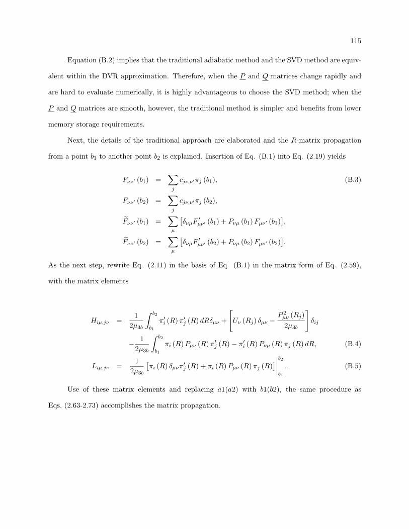
115

Equation (B.2) implies that the traditional adiabatic method and the SVD method are equiv-

alent within the DVR approximation. Therefore, when the P and Q matrices change rapidly and

are hard to evaluate numerically, it is highly advantageous to choose the SVD method; when the

P and Q matrices are smooth, however, the traditional method is simpler and benefits from lower

memory storage requirements.

Next, the details of the traditional approach are elaborated and the R-matrix propagation

from a point b1 to another point b2 is explained. Insertion of Eq. (B.1) into Eq. (2.19) yields

Fνν′ (b1) =∑j

cjν,ν′πj (b1), (B.3)

Fνν′ (b2) =∑j

cjν,ν′πj (b2),

Fνν′ (b1) =∑µ

[δνµF

′µν′ (b1) + Pνµ (b1)Fµν′ (b1)

],

Fνν′ (b2) =∑µ

[δνµF

′µν′ (b2) + Pνµ (b2)Fµν′ (b2)

].

As the next step, rewrite Eq. (2.11) in the basis of Eq. (B.1) in the matrix form of Eq. (2.59),

with the matrix elements

Hiµ,jν =1

2µ3b

∫ b2

b1

π′i (R)π′j (R) dRδµν +

[Uν (Rj) δµν −

P 2µν (Rj)

2µ3b

]δij

− 1

2µ3b

∫ b2

b1

πi (R)Pµν (R)π′j (R)− π′i (R)Pνµ (R)πj (R) dR, (B.4)

Liµ,jν =1

2µ3b

[πi (R) δµνπ

′j (R) + πi (R)Pµν (R)πj (R)

]∣∣∣∣b2b1

. (B.5)

Use of these matrix elements and replacing a1(a2) with b1(b2), the same procedure as

Eqs. (2.63-2.73) accomplishes the matrix propagation.

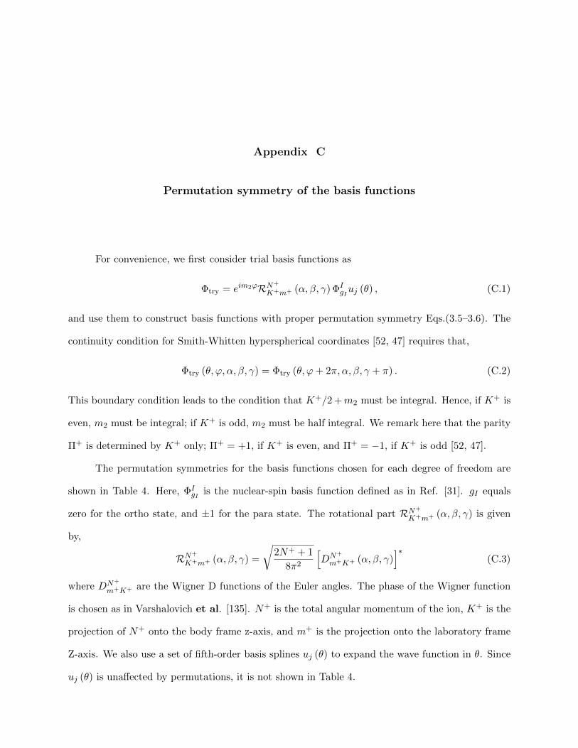
Appendix C

Permutation symmetry of the basis functions

For convenience, we first consider trial basis functions as

Φtry = eim2ϕRN+

K+m+ (α, β, γ) ΦIgIuj (θ) , (C.1)

and use them to construct basis functions with proper permutation symmetry Eqs.(3.5–3.6). The

continuity condition for Smith-Whitten hyperspherical coordinates [52, 47] requires that,

Φtry (θ, ϕ, α, β, γ) = Φtry (θ, ϕ+ 2π, α, β, γ + π) . (C.2)

This boundary condition leads to the condition that K+/2 +m2 must be integral. Hence, if K+ is

even, m2 must be integral; if K+ is odd, m2 must be half integral. We remark here that the parity

Π+ is determined by K+ only; Π+ = +1, if K+ is even, and Π+ = −1, if K+ is odd [52, 47].

The permutation symmetries for the basis functions chosen for each degree of freedom are

shown in Table 4. Here, ΦIgI

is the nuclear-spin basis function defined as in Ref. [31]. gI equals

zero for the ortho state, and ±1 for the para state. The rotational part RN+

K+m+ (α, β, γ) is given

by,

RN+

K+m+ (α, β, γ) =

√2N+ + 1

8π2

[DN+

m+K+ (α, β, γ)]∗

(C.3)

where DN+

m+K+ are the Wigner D functions of the Euler angles. The phase of the Wigner function

is chosen as in Varshalovich et al. [135]. N+ is the total angular momentum of the ion, K+ is the

projection of N+ onto the body frame z-axis, and m+ is the projection onto the laboratory frame

Z-axis. We also use a set of fifth-order basis splines uj (θ) to expand the wave function in θ. Since

uj (θ) is unaffected by permutations, it is not shown in Table 4.

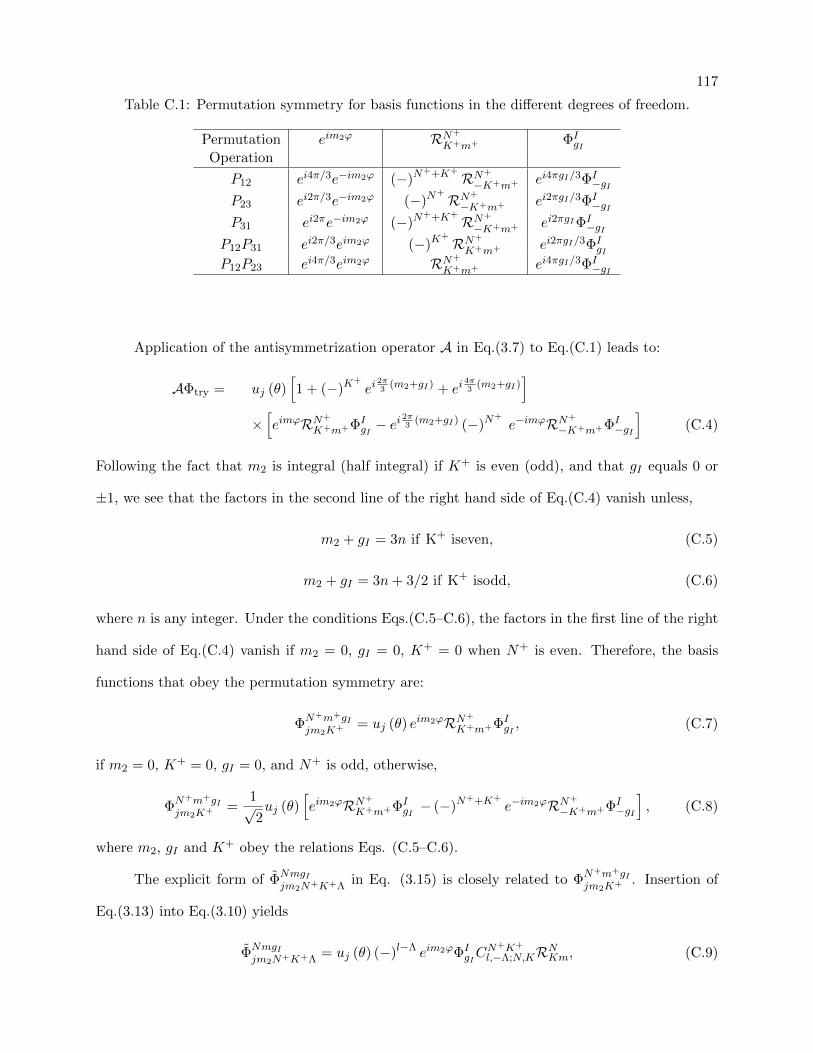
117

Table C.1: Permutation symmetry for basis functions in the different degrees of freedom.

Permutation eim2ϕ RN+

K+m+ ΦIgI

Operation

P12 ei4π/3e−im2ϕ (−)N++K+

RN+

−K+m+ ei4πgI/3ΦI−gI

P23 ei2π/3e−im2ϕ (−)N+

RN+

−K+m+ ei2πgI/3ΦI−gI

P31 ei2πe−im2ϕ (−)N++K+

RN+

−K+m+ ei2πgIΦI−gI

P12P31 ei2π/3eim2ϕ (−)K+

RN+

K+m+ ei2πgI/3ΦIgI

P12P23 ei4π/3eim2ϕ RN+

K+m+ ei4πgI/3ΦI−gI

Application of the antisymmetrization operator A in Eq.(3.7) to Eq.(C.1) leads to:

AΦtry = uj (θ)[1 + (−)K

+

ei2π3

(m2+gI) + ei4π3

(m2+gI)]

×[eimϕRN+

K+m+ΦIgI− ei

2π3

(m2+gI) (−)N+

e−imϕRN+

−K+m+ΦI−gI

](C.4)

Following the fact that m2 is integral (half integral) if K+ is even (odd), and that gI equals 0 or

±1, we see that the factors in the second line of the right hand side of Eq.(C.4) vanish unless,

m2 + gI = 3n if K+ iseven, (C.5)

m2 + gI = 3n+ 3/2 if K+ isodd, (C.6)

where n is any integer. Under the conditions Eqs.(C.5–C.6), the factors in the first line of the right

hand side of Eq.(C.4) vanish if m2 = 0, gI = 0, K+ = 0 when N+ is even. Therefore, the basis

functions that obey the permutation symmetry are:

ΦN+m+gIjm2K+ = uj (θ) eim2ϕRN+

K+m+ΦIgI, (C.7)

if m2 = 0, K+ = 0, gI = 0, and N+ is odd, otherwise,

ΦN+m+gIjm2K+ =

1√2uj (θ)

[eim2ϕRN+

K+m+ΦIgI− (−)N

++K+

e−im2ϕRN+

−K+m+ΦI−gI

], (C.8)

where m2, gI and K+ obey the relations Eqs. (C.5–C.6).

The explicit form of ΦNmgIjm2N+K+Λ

in Eq. (3.15) is closely related to ΦN+m+gIjm2K+ . Insertion of

Eq.(3.13) into Eq.(3.10) yields

ΦNmgIjm2N+K+Λ

= uj (θ) (−)l−Λ eim2ϕΦIgICN

+K+

l,−Λ;N,KRNKm, (C.9)

118

with K = K+ + Λ, if m2 = 0, gI = 0, K+ = 0 and N+ is odd. Otherwise,

ΦNmgIjm2N+K+Λ

=uj (θ)√

2(−)l−Λ

[eim2ϕΦI

gICN

+K+

l,−Λ;N,KRNKm − (−)N++K+

e−im2ϕΦI−gIC

N+−K+

l,−Λ;N,KRNKm

],

(C.10)

where K = −K+ + Λ.

Appendix D

Body-frame quantum defect matrix elements

The form of reaction matrix K describing the Jahn-Teller coupling of the p-wave electron

can be written as

KΛΛ′ =

K00 K01 K0−1

K10 K11 K1−1

K−10 K−11 K−1−1

. (D.1)

In perturbation theory, the matrix elements of the reaction matrix near the equilibrium position

obey,

KΛΛ′ ≈ −π∫dr′fεlΛ

(r′)fεlΛ′

(r′)

(D.2)

×∫dω′eY

∗lΛ

(θ′e, ϕ

′e

)∆Ve

(Q; re

′)YlΛ′ (θ′e, ϕ′e) ,where ∆Ve = Ve (Q; re

′)− Ve (Q = 0; re′), and Ve (Q, r′e) is the interaction between the ion and the

Rydberg electron excluding the Coulomb potential, Q are the vibrational symmetry coordinates,

and re′ = r′, θ′e, ϕ′e are the spherical coordinates of the electron in the body-frame. fεlΛ (r′) is

the regular phase-renormalized Coulomb wave function defined by, fεlΛ = fεl cos (πµΛΛ (Q = 0))−

gεl sin (πµΛΛ (Q = 0)), where fεl, gεl are the usual Coulomb wave functions with energy ε and

angular momentum l. µΛΛ (Q = 0) are the constant zero-order term of the diagonal quantum

defect matrix elements.

To explore the symmetry properties of KΛΛ′ , we write the Taylor expansion in terms of

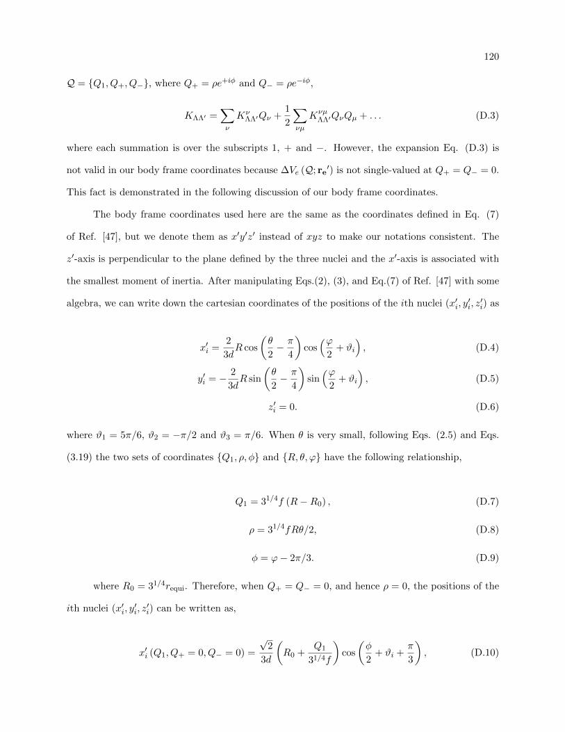
120

Q = Q1, Q+, Q−, where Q+ = ρe+iφ and Q− = ρe−iφ,

KΛΛ′ =∑ν

KνΛΛ′Qν +

1

2

∑νµ

KνµΛΛ′QνQµ + . . . (D.3)

where each summation is over the subscripts 1, + and −. However, the expansion Eq. (D.3) is

not valid in our body frame coordinates because ∆Ve (Q; re′) is not single-valued at Q+ = Q− = 0.

This fact is demonstrated in the following discussion of our body frame coordinates.

The body frame coordinates used here are the same as the coordinates defined in Eq. (7)

of Ref. [47], but we denote them as x′y′z′ instead of xyz to make our notations consistent. The

z′-axis is perpendicular to the plane defined by the three nuclei and the x′-axis is associated with

the smallest moment of inertia. After manipulating Eqs.(2), (3), and Eq.(7) of Ref. [47] with some

algebra, we can write down the cartesian coordinates of the positions of the ith nuclei (x′i, y′i, z′i) as

x′i =2

3dR cos

(θ

2− π

4

)cos(ϕ

2+ ϑi

), (D.4)

y′i = − 2

3dR sin

(θ

2− π

4

)sin(ϕ

2+ ϑi

), (D.5)

z′i = 0. (D.6)

where ϑ1 = 5π/6, ϑ2 = −π/2 and ϑ3 = π/6. When θ is very small, following Eqs. (2.5) and Eqs.

(3.19) the two sets of coordinates Q1, ρ, φ and R, θ, ϕ have the following relationship,

Q1 = 31/4f (R−R0) , (D.7)

ρ = 31/4fRθ/2, (D.8)

φ = ϕ− 2π/3. (D.9)

where R0 = 31/4requi. Therefore, when Q+ = Q− = 0, and hence ρ = 0, the positions of the

ith nuclei (x′i, y′i, z′i) can be written as,

x′i (Q1, Q+ = 0, Q− = 0) =

√2

3d

(R0 +

Q1

31/4f

)cos

(φ

2+ ϑi +

π

3

), (D.10)

121

y′i (Q1, Q+ = 0, Q− = 0) =

√2

3d

(R0 +

Q1

31/4f

)sin

(φ

2+ ϑi +

π

3

), (D.11)

zi (Q1, Q+ = 0, Q− = 0) = 0. (D.12)

These equations show that the positions of the three nuclei can not be expressed by Q1,

Q+ and Q− when ρ = 0, and hence the expansion Eq. (D.3) is not valid as ∆Ve (Q; re′) is not

single-valued at Q+ = Q− = 0 and therefore is not infinitely differentiable. However, if we define

another set of x′, y′, z′ axis by a passive rotation through φ/2 about z′-axes, the positions of nuclei

have defined values when Q+ = Q− = 0 in this new frame:

x′i (Q1, Q+ = 0, Q− = 0) =

√2

3d

(R0 +

Q1

31/4f

)cos

(ϑi +

2π

3

), (D.13)

y′i (Q1, Q+ = 0, Q− = 0) =

√2

3d

(R0 +

Q1

31/4f

)sin

(ϑi +

2π

3

), (D.14)

z′i (Q1, Q+ = 0, Q− = 0) = 0. (D.15)

Hence, the following expansion is valid,

KΛΛ′ =∑ν

KνΛΛ′Qν +

1

2

∑νµ

KνµΛΛ′QνQµ + . . . , (D.16)

and therefore using the analysis of Longuet-Higgins [136] in which KΛΛ is expanded to third order

in Q1 and second order in ρ, gives:

KΛΛ = K1ΛΛQ1 + K11

ΛΛQ21 + K111

ΛΛQ31 + K+−

ΛΛ ρ2. (D.17)

We also have

KΛΛ±1 = KΛ±1Λ = 0, (D.18)

and

KΛΛ±2 = KΛ±2Λ = K1ΛΛ±2ρe

∓iφ, (D.19)

to first order in ρ. The matrix elements of KΛΛ′ also obey

KΛΛ′ ≈ −π∫dr′fεlΛ

(r′)fεlΛ′

(r′)

(D.20)

×∫dω′eY

∗lΛ

(θ′e, ϕ

′e

)Ve(Q, re′

)YlΛ′

(θ′e, ϕ

′e

),

122

where we use the tilde notation to stress that these are expressed in terms of coordinates in the

new frame. The rotation to the new frame from our original one has the following effects: θe = θe

and ϕe = ϕe − φ/2. Hence a comparison with Eq. (D.2) gives

KΛΛ′ = KΛΛ′ei(Λ−Λ′)φ/2. (D.21)

Because the reaction matrix K and quantum defect matrix µ are related by µ = µ (Q = 0) +

arctan (K) /π ≈ µ (Q = 0) + K/π + O(K3)/π + . . ., at least to first order, the K matrix and µ

matrix have the same symmetry properties, and hence we write the form of µ matrix as Eq.(3.18)

and Eqs.(3.23-3.25).

Appendix E

Effective adiabatic potentials

The effective potentials shown in Fig. 1 (a) of the main text are very complicated, making

identification of the important physics challenging. For that reason, this section presents some

details of our work that not only give support to our physical interpretation of the nature of the

three-body parameter but also show how some important nonuniversal aspects appear in the hyper-

spherical adiabatic representation. In fact, Fig. E.1 shows some of the most drastic nonadiabatic

effects found in our calculations. The model proposed in Ref. [16] is also considered, and we show

that this model offers an interesting qualitative picture; but since incorporation of corrections to

that model diminishes its accuracy in the three-body parameter universality, its agreement with

experiment might be fortuitous.

We first consider the validity of the single-channel adiabatic hyperspherical approximation

and point out the manner in which some important nonuniversal features manifest themselves.

Figure E.1 shows the results for Uν(R) and Wν(R) obtained from three different two-body poten-

tial models. Figures E.1 (a) and (b) show the results for the potential models vaλ(λ = λ∗2) and

vaλ(λ = λ∗10) [Eq. (5.3)], respectively, while Fig. E.1 (c) shows the results obtained for vsch(D = D∗6)

[Eq. (5.2)]. The most striking aspect of these figures is that Uν(R) and Wν(R) are substantially dif-

ferent, meaning that the nonadiabatic couplings Pνν′(R) and Qνν′(R) are important near R = rvdW.

Therefore, it is clear that one needs to go beyond a single channel approximation in order to de-

scribe the three-body observables. It is worth noting that the nonadiabatic couplings originate from

the hyperradial kinetic energy. Their large values are thus consistent with our physical picture in

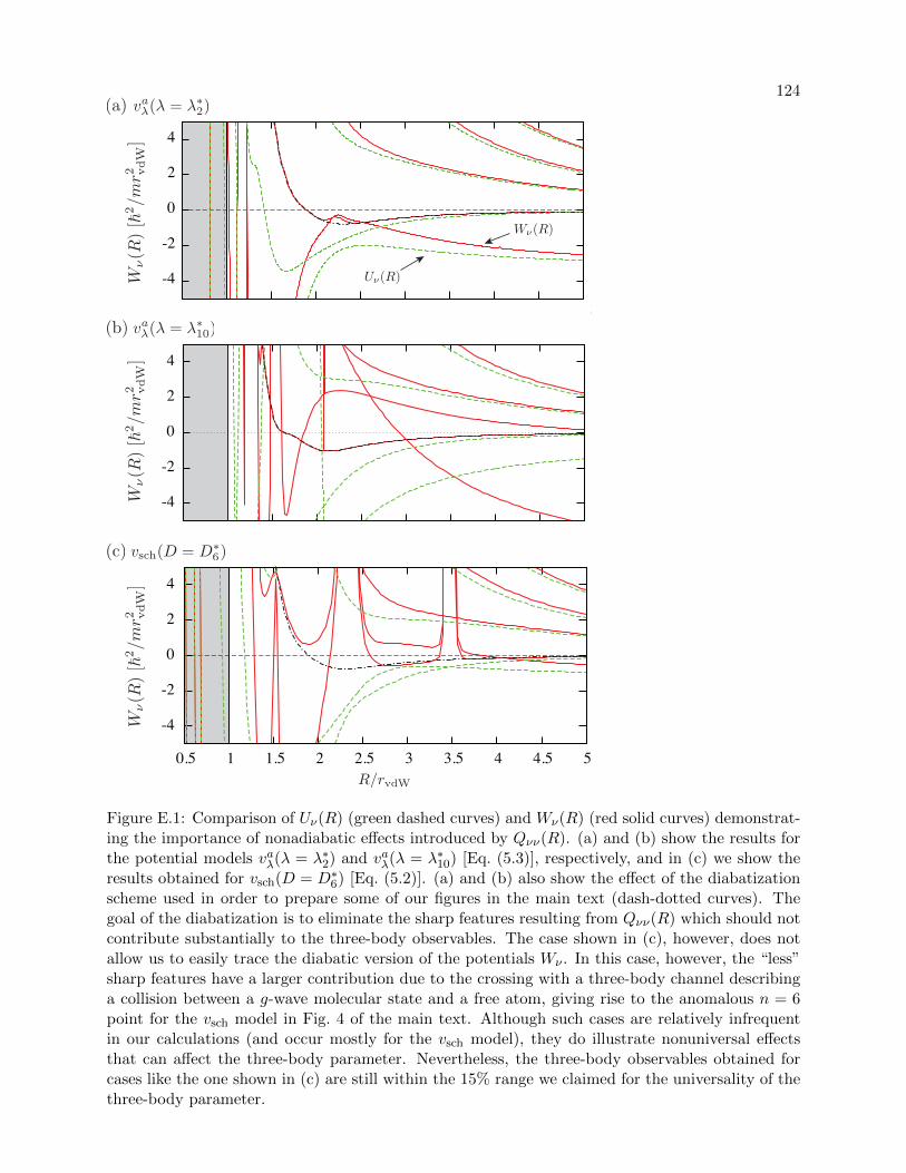
124

-4

-2

0

2

4

0.5 1 1.5 2 2.5 3 3.5 4 4.5 5

-4

-2

0

2

4

0.5 1 1.5 2 2.5 3 3.5 4 4.5 5

-4

-2

0

2

4

0.5 1 1.5 2 2.5 3 3.5 4 4.5 5

Figure E.1: Comparison of Uν(R) (green dashed curves) and Wν(R) (red solid curves) demonstrat-ing the importance of nonadiabatic effects introduced by Qνν(R). (a) and (b) show the results forthe potential models vaλ(λ = λ∗2) and vaλ(λ = λ∗10) [Eq. (5.3)], respectively, and in (c) we show theresults obtained for vsch(D = D∗6) [Eq. (5.2)]. (a) and (b) also show the effect of the diabatizationscheme used in order to prepare some of our figures in the main text (dash-dotted curves). Thegoal of the diabatization is to eliminate the sharp features resulting from Qνν(R) which should notcontribute substantially to the three-body observables. The case shown in (c), however, does notallow us to easily trace the diabatic version of the potentials Wν . In this case, however, the “less”sharp features have a larger contribution due to the crossing with a three-body channel describinga collision between a g-wave molecular state and a free atom, giving rise to the anomalous n = 6point for the vsch model in Fig. 4 of the main text. Although such cases are relatively infrequentin our calculations (and occur mostly for the vsch model), they do illustrate nonuniversal effectsthat can affect the three-body parameter. Nevertheless, the three-body observables obtained forcases like the one shown in (c) are still within the 15% range we claimed for the universality of thethree-body parameter.

125

which the local kinetic energy increases and generates the repulsive barrier in our effective poten-

tials. It is also worth mentioning that since the three-body repulsive barrier prevents particles from

approaching to small distances, the question of whether or not the short range physics actually

changes as a function of the external magnetic field (as in experiments in ultracold quantum gases)

[137] can not be directly answered by observing features related to Efimov physics.