hypernuclear bound states with two ›-particles

HYPERNUCLEAR BOUND STATES WITH TWO

Λ-PARTICLES

by

JONATHAN GROBLER

submitted in accordance with the requirements for the degreeof

MASTER OF SCIENCE

in the subject

PHYSICS

at the

UNIVERSITY OF SOUTH AFRICA

SUPERVISOR: PROF S A RAKITYANSKY

NOVEMBER 2009

University of South Africa ETD Grobler, J. (2010)

Declaration

I, the undersigned, declare that Hypernuclear Bound States with two Λ-

particles is my own work and that all the sources that I have used or quoted

have been indicated and acknowledged by means of complete references. This

work has not been previously submitted, either in its entirety, or in part, for

a degree at this, or at any another tertiary institution.

Signature: Date:

i


Summary

The double Λ hypernuclear systems are studied within the context of the

hyperspherical approach. Possible bound states of these systems are sought

as zeros of the corresponding three-body Jost function in the complex energy

plane. Hypercentral potentials for the system are constructed from known

potentials in order to determine bound states of the system. Calculated

binding energies for double-Λ hypernuclei having A = 4 − 20, are presented.

Keywords: Jost function, bound state, Λ-particle, Λ-Λ interaction, hyper-

nucleus, hyperspherical harmonics, complex rotation, hypercentral potential

ii


Acknowledgements

My heartfelt gratitude and appreciation goes to the following persons for

their guidance and support:

My wife Ruth, Michael, Rachel and Prof. S. A. Rakityansky.

In loving memory of my mother.

iii


List of Figures

3.1 Spatial configuration of two Λ-particles in the nucleus. . . . . 15

3.2 r1 and r2 in the polar plane. r1 and r2 vary over infinite intervals. 16

4.1 ΛΛ-potential. The potential decays exponentially, approaches

a negligible value at about 0.7 fm. . . . . . . . . . . . . . . . . 38

4.2 Λ-nucleus potential for a well depth of W = −28.0 MeV, mass

number of A = 15 and diffusivity a = 0.6 fm. The potential

falls off quite rapidly beyond the hypernuclear surface and

approaches a negligibly small value at ≈ 5 fm. . . . . . . . . . 40

4.3 Hypercentral potentials for A = 4 − 20. The minimum values

of the potentials for A = 4 and A = 20 are about 2.5 fm and

2.8 fm, respectively. Note the increase in depth, ≈ 17 MeV,

with increasing mass number for A = 4 − 20. The minimum

of the hypercentral potential for A = 20 is shifted by ≈ 0.5

fm relative to that for A = 4. The curves for A = 5 − 19 lie

between the two curves for A = 4 and A = 20. . . . . . . . . . 45

4.4 Deformed contour showing path of integration for (4.55) with

complex energies. . . . . . . . . . . . . . . . . . . . . . . . . . 46

iv


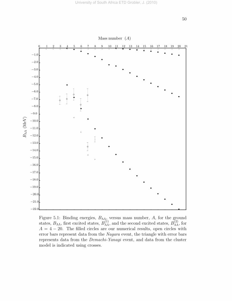
5.1 Binding energies, BΛΛ, versus mass number, A, for the ground

states, BΛΛ, first excited states, B(1)ΛΛ, and the second excited

states, B(2)ΛΛ, for A = 4−20. The filled circles are our numerical

results, open circles with error bars represent data from the

Nagara event, the triangle with error bars represents data from

the Demachi-Yanagi event, and data from the cluster model

is indicated using crosses. . . . . . . . . . . . . . . . . . . . . 50

v


List of Tables

2.1 Binding energies for two Λ-hyperons, BΛΛ, and Λ-Λ interaction

energy, ∆BΛΛ. The errors on BΛΛ do not include those of the

binding energies of single hypernuclei. Values are taken from

Ref. [7]. . . . . . . . . . . . . . . . . . . . . . . . . . . . . . . 8

2.2 Calculated energies of the ground states of A = 7 − 10 based

on the (α + x+ Λ + Λ) four-body model (x = 0, n, p, d, t, 4ΛHe

and α). Values are taken from Ref. [12] . . . . . . . . . . . . . 8

2.3 Properties of the Λ-particle. Values are taken from Ref. [21]. . 9

2.4 Λ decay modes. Values are taken from Ref. [22] . . . . . . . . 10

4.1 Parameters of the ΛΛ-potential. The strength of the long-

range part of the potential is reduced by multipliying by the

factor γ = 0.6598 in order to ensure agreement with experi-

mental results [11]. . . . . . . . . . . . . . . . . . . . . . . . . 37

5.1 Binding energies for the ground states, BΛΛ, first excited states,

B(1)ΛΛ, and the second excited states, B

(2)ΛΛ, for A = 4 − 20. . . . 49

6.1 Estimated binding energies for the ground states, BΛΛ, first

excited states, B(1)ΛΛ, and the second excited states, B

(2)ΛΛ, for

A = 9 − 20. . . . . . . . . . . . . . . . . . . . . . . . . . . . . 54

vi


Contents

1 Introduction 1

2 Hypernuclear Physics 7

2.1 The Λ-particle . . . . . . . . . . . . . . . . . . . . . . . . . . . 9

2.2 The Hypernucleus . . . . . . . . . . . . . . . . . . . . . . . . . 11

3 Model 14

3.1 Two Λ-particles in the Nucleus . . . . . . . . . . . . . . . . . 14

3.2 The Hyperspherical Coordinate System . . . . . . . . . . . . . 15

3.3 Hamiltonian of the System . . . . . . . . . . . . . . . . . . . . 16

3.3.1 Volume Element . . . . . . . . . . . . . . . . . . . . . 21

3.4 Schrodinger Equation of the System . . . . . . . . . . . . . . . 23

4 Method of Solution 27

4.1 The Jost Function . . . . . . . . . . . . . . . . . . . . . . . . 27

4.2 Three-body Jost Matrix . . . . . . . . . . . . . . . . . . . . . 29

4.3 Method of Locating Bound States . . . . . . . . . . . . . . . . 33

4.4 Minimal Approximation . . . . . . . . . . . . . . . . . . . . . 34

vii


viii

4.5 ΛΛ-Potential . . . . . . . . . . . . . . . . . . . . . . . . . . . 37

4.6 Λ-Nucleus Potential . . . . . . . . . . . . . . . . . . . . . . . . 39

4.7 Total Potential . . . . . . . . . . . . . . . . . . . . . . . . . . 41

4.8 Complex Rotation . . . . . . . . . . . . . . . . . . . . . . . . 45

5 Results and Discussion 48

6 Conclusion 53


Chapter 1

Introduction

Until 1947, it was thought that the only building blocks of nuclei were pro-

tons and neutrons, bound together by nuclear forces. It was in this year

that the pioneering work of C.F. Powell [1], who developed the nuclear emul-

sion technique, produced evidence for the existence of mesons. The evidence

produced by Powell included what is now known as the π meson. These dis-

coveries initiated elementary particle physics as a separate branch of physics

and established the nuclear emulsion technique as a recognised method in

the search for elementary particles.

In 1952, using the nuclear emulsion technique, Marian Dansyz and Jerzy

Pniewski [2] came across a surprising case of two stars connected by a thick

track. Their analysis led them to conclude that the experimental evidence

depicted a hypernucleus, in their particular case, a nucleus consisting of a Λ-

hyperon and nucleons. Up to, and until 1955, many other cases of hypernuclei

were announced [3]. These new dicoveries posed new fundamental questions

concerning the existence, creation and disintegration of the Λ-hyperon, ques-

tions which would pave the way for exciting new developments in the area

of elementary particles and their interactions.

1


2

The first double hypernucleus was discovered in Warsaw, in 1962 [4], using

a nuclear emulsion irradadiated by a beam of kaons (K−-mesons), and the

second at Brookhaven National Laboratory in 1966 [5]. Further searches

for double hypernuclei, including the use of spectrometers, were unsuccessful

with none being discovered for over thirty years. Finally, in 1991, in an

experiment performed with K−-beams at the KEK Proton Synchorotron in

Tokyo [6], the next double hypernucleus was discovered.

Hypernuclei are of great importance as they provide the only means of ob-

taining information on the Λ-Λ interaction, notably the binding energy of

two Λ-hyperons, BΛΛ, and the Λ-Λ interaction energy, ∆BΛΛ. The interac-

tion energy can be obtained from the mass of double hypernuclei using the

formula [7]

∆BΛΛ( AΛΛZ) = BΛΛ( A

ΛΛZ) − 2BΛ(A−1ΛΛ Z), (1.1)

where the superscript A indicates the total number of baryons. For example,

6ΛΛHe is a bound system (ppnnΛΛ).

The Λ-Λ interaction may also provide valuable insight into the details of

neutron stars [8], where hyperons are seen to play an important role in the

core region of these stars. The structure of the hypernucleus also provides

valuable information on the hyperon-nucleon interaction. Little is currently

known about hyperon-nucleon interactions with more theoretical and exper-

imental work being required for an accurate description of them. There are

numerous reasons which motivate hypernuclear physics research: A detailed,

consistent understanding of the quark aspect for bayron-bayron interactions

is needed; extension of the three-dimensional hypernuclear chart; impurity

effects in nuclear structure; nuclear medium effects of bayrons; the study of


3

strangeness in astro physics; and the production of exotic hypernuclei beyond

the normal neutron/proton drip lines.

The binding energies of double hypernuclei have been studied as far back as

1960, with the aim of gaining more information on the Λ-Λ interaction [9].

These studies were theoretical in nature and unsuccessful in accurately de-

termining the binding energies of two hyperons. Recent experimental work

performed at the KEK proton synchrotron [7], using the 1.66 GeV/c sepa-

rated K− meson beam, unveiled important information about the 6ΛΛHe dou-

ble hypernucleus. An event of seminal importance, a mesonically decaying

double hypernucleus, was identified and termed the “Nagara” event [7]. The

results of the experimental work provided the first-ever, reliable information

on the binding energy of 6ΛΛHe.

After the Nagara event, there were numerous other attempts to establish

whether 4ΛΛHe is a stable bound state against strong decay [10, 11]. The

inclusion of a set of baryon-baryon interactions, consistent with experimental

data, was used [10] to predict a stable state of 4ΛΛH. The results of this work

showed that with the inclusion of a set of baryon-baryon intractions among

the octet baryons in the S = 0,−1 and −2 strangeness sectors (which is

consistent with the Nagara event as well as the experimental binding energies

of S = 0 and −1 s-shell hypernuclei) one can predict a stable bound state

of 4ΛΛHe. Bound state solutions for 4

ΛΛH, 5ΛΛH, 5

ΛΛHe were also determined as

well as Λ-Λ separation energies of A = 4, S = −2 hypernuclei [10].

In addition to the Nagara event, the “Demachi-Yanagi” event [12] revealed

more information about hypernuclei. The binding energy of 10ΛΛBe was eval-

uated as BΛΛ = 12.33+0.35−0.21 MeV. However, it was not certain at the time

whether the state observed was a ground state or an excited state. Later,


4

systematic four-body calculations for 6ΛΛHe were performed [13] which showed

that the Demachi-Yanagi event may be interptreted as the 2+ state of 10ΛΛBe.

The microscopic cluster model is found to be most useful in understanding

the structure of light hypernuclei and is established as an important feature

of hypernuclear systems and has been successful in describing the shell struc-

ture of hypernuclei [14, 15, 16]. In the cluster model, antisymmetrization of

nucleons is properly taken into account with wave functions treating con-

stituent clusters as composites. The cluster model has also been successful

in describing the nuclear response to the addition of the Λ-hyperon which is

uninhibited by the Pauli blocking effect [12].

The Gaussian expansion method [17] has enjoyed recent success in the area

of three- and four-body structure calculations. The method employs a set

of Gaussian basis functions which form a set in coordinate space. These

basis functions enable description of both the short-range and the long-range

asymptotic behaviour of the wave function for bound systems and scattering

states [12].

Despite the success of the Gaussian expansion method and the Cluster model,

the results of these methods are acknowledged as predictions, especially the

energy spectra of double Λ with A = 6 − 10. The Nagara and Demachi-

Yanagi events remain the most accurate and reliable sources of experimental

evidence for the binding energies of double Λ-hypernuclei. As these results

serve as the only reliable source of data, they impose natural constraints on

binding energy calculations of 6ΛΛHe and 10

ΛΛBe. Due to the lack of confirmed

experimental evidence, forthcoming experiments are expected to reveal fur-

ther aspects of hypernuclear systems [18].

What about scattering experiments using Λ-particles, one may ask. Un-


5

fortunately, due to the short lifetime of the Λ-particle, its scarcity and low

intensity beams that can be obtained from them, it is difficult to conduct scat-

tering experiments using Λ-particles. Targets which consist of Λ-particles are

not readily available, which makes scattering experiments difficult. Hyperon-

nucleon interactions and hyperon-hyperon scattering in free space is also very

difficult.

In recent work [19], three-body resonances of the Λnn and ΛΛn hypernuclear

systems were sought as zeros of the corresponding Jost functions. The hy-

perspherical approach with local two-body S-wave potentials describing nn,

Λn, and Λ-Λ interactions was used. It was found that the positions of the

resonances were sensitive to the choice of the Λn-potential. It was also found

that bound states appear when the potential strength was increased by ap-

proximately 50%, implying that the Jost function zeros crossed the threshold

and moved into the real negative axis. The method was successful in locat-

ing resonances, but did not include a search for bound states of hypernuclei

containing two Λ-hyperons, which is the subject of this work.

We aim to develop a theoretical model of a ΛΛ hypernuclear system, with a

view to determining how strong the the Λ-Λ interaction is based on compar-

ison with the experimental results obtained in the Nagara and the Demachi-

Yangi events. We also aim to determine binding energies for A = 4 − 20

hypernuclei. Our calculations reproduce the binding energy of 6ΛΛHe and

therefore we hope that the results which we obtained for the other ΛΛ hy-

pernuclei are also realistic. They can be considered as estimates for future

experiments.

We consider the ΛΛ-nucleus system in the three-body model: nuclear core

plus two Λ-particles. The three-body wave function is expanded in terms of


6

hyperspherical harmonics. The resulting system of hyperradial equations is

truncated to a single Schrodinger-like equation.

We reduce the second-order Schrodinger Equation of the system to a single

pair of first-order differential equations. Each of these first-order differential

equations is then solved numerically as a boundary-value problem to deter-

mine the Jost function. The Jost function is then used to locate the bound

states for the hypernuclear system.

This work is structured as follows: In Chapter 2 we describe the Λ-particle

and the hypernucleus. In Chapter 3 we develop a model which consists of

two Λ-particles in the nucleus. Here we derive the Hamiltonian and the

Schrodinger Equation for the system. In Chapter 4 we describe the Jost

function method for solving the Schrodinger Equation derived in Chapter 3,

methods for locating bound states for ΛΛ hypernuclear systems, the Minimal

Approximation and Complex Rotation. In Chapter 5 we present and discuss

the results of our method, and in Chapter 6 we state the conclusion.


Chapter 2

Hypernuclear Physics

The Nagara event involved the production of Ξ−-hyperons, measurements

of the position and angles of entry of Ξ−-hyperons, and analysis of the ex-

perimental results using measured lengths and angles of the tracks. The

kinematics of all possible decay modes was also investigated. The event was

interpreted as the sequential weak decay of 6ΛΛHe, the lightest triply-closed

s-shell nuclear system [7]. The most probable weighted mean value for the

binding energy was determined, BΛΛ = 7.25 ± 0.19+0.18−0.11 MeV, and the inter-

action energy, ∆BΛΛ = 1.10 ± 0.20+0.18−0.11 MeV, was also determined. Binding

energies for two Λ-hyperons, BΛΛ, and the Λ-Λ interaction energy, ∆BΛΛ,

were also presented [7]. These are given in Table 2.1.

Four-body cluster model calculations have been extensively used to study the

structure of ΛΛ hypernuclear systems. In these structure calculations [12],

the ΛΛ hypernuclear systems 7ΛΛHe, 7

ΛΛLi, 8ΛΛLi, 9

ΛΛLi, 9ΛΛBe, and 10

ΛΛBe were

studied within the framework of an (α + x + Λ + Λ) four-body model with

x = 0, n, p, d, t, 4ΛHe and α, respectively. Here, the d, t( 3He) and α clusters

were assumed to be inert, having the (0s)2, (0s)3, and (0s)4 shell-model

configurations, respectively, with spins s(= 1, 1/2, or 0), respectively.

7


8

Cluster models have also been extended to more general cases where the

nuclear core is well represented. Recent calculations for the A = 7 − 9

Λ species have been presented for the first time [12] and a summary of the

calculated ground state energies for ΛΛ hypernuclear species is given in Table

2.2.

Hypernucleus BΛΛ [MeV] ∆BΛΛ [MeV]

5ΛΛHe 7.1 ± 0.5 2.4 ± 0.5

6ΛΛHe 6.9 ± 0.6 0.6 ± 0.6

7ΛΛHe 6.3 ± 0.7 −2.0 ± 0.7

8ΛΛHe 7.7 ± 0.8 −6.3 ± 0.8

9ΛΛHe 13.4 ± 0.5 −0.9 ± 0.5

9ΛΛHe 6.4 ± 0.8 −7.9 ± 0.8

Table 2.1: Binding energies for two Λ-hyperons, BΛΛ, and Λ-Λ interactionenergy, ∆BΛΛ. The errors on BΛΛ do not include those of the binding energiesof single hypernuclei. Values are taken from Ref. [7].

Hypernucleus BΛΛ [MeV]

7ΛΛLi 9.45

8ΛΛLi 11.44

9ΛΛLi 14.55

10ΛΛBe 15.14

Table 2.2: Calculated energies of the ground states of A = 7 − 10 based onthe (α + x + Λ + Λ) four-body model (x = 0, n, p, d, t, 4

ΛHe and α). Valuesare taken from Ref. [12]


9

2.1 The Λ-particle

The first Λ-particle was discovered in 1947 during research of cosmic ray

interactions [20]. This led to a number of further discoveries, notably the

principle of the conservation of strangeness and the strange quark.

The Λ-particle contains an up quark, a down quark, and a strange quark.

The Λ-particle is the lightest of the hyperons with a rest mass of 1115.684

MeV/c2 and a mean lifetime of 2.60× 10−10s, which is consistent with weak

decay [21]. The Λ-particle also has the properties listed in Table 2.3.

Λ-particle property Quantum Number

Isospin (I) 0

Spin (Parity) 1/2+

Charge (Q) 0

Strangeness (S) −1

Charm (C) 0

Bottomness (B) 0

Table 2.3: Properties of the Λ-particle. Values are taken from Ref. [21].

The Λ-particle decays into a nucleon through a weak interaction process.

The strangeness quantum number, S, changes by one unit during the decay

process, hence S is not conserved during the process. The decay modes of

the Λ-hyperon are given in Table 2.4

As the Λ-particle is shortlived, the study of Λ-particles bound in the nucleus

may provide valuable information about the interaction between hyperons

(Y) and nucleons (N).

As we know, neither beams nor targets of Λ-particles are readily available,


10

Λ decay mode Fraction [%]

p+ π− (63.9 ± 0.5)

n+ π0 (35.8 ± 0.5)

n + γ (1.75 ± 0.15) × 10−3

p+ π− + γ (8.4 ± 1.4) × 10−4

p+ e− + νe (8.32 ± 0.14) × 10−4

p+ µ− + νµ (1.57 ± 0.35) × 10−4

Table 2.4: Λ decay modes. Values are taken from Ref. [22]

which makes scattering experiments with Λ-particles difficult. However, in

practice Λ-particles may be produced by passing a beam of kaons into a

liquid hydrogen target [21]. In this process, Λ-particles are produced in the

reaction

K− + p→ AΛX + π+,

where p denotes the proton and π+ the π-meson with positive electric charge.

As with nn scattering, Λp scattering may be characterized by two parame-

ters, the scattering length a and the effective range r0. The scattering data

obtained favor the values a = −1.8 ± 0.2 fm and r0 = 3.16 ± 0.52 fm [21].

Another way of examining nuclear interactions of Λ-particles is through hy-

pernuclei where a neutron is replaced with a Λ-particle. This is achieved in

scattering experiments using a beam of K− and with nuclei as targets [21].

This kind of reaction is indicated by

K− + n→ AΛX + π−,

where Λ-particles produced at low momentum have a high probability of

remaining bound to the nucleus. As the Λ-particles are not limited by the


11

Pauli principle, they can drop quickly to the 1s shell state, despite the fact

that there may already be two neutrons in that state. The Λ-particle may

stay in the 1s state until it decays, according to

Λ → p+ π−,

or

Λ → n+ π0.

The Λ-particle may alternatively undergo a strangeness-changing weak reac-

tion with either the proton or the neutron

Λ + n→ n+ n

Λ + p→ n+ p.

2.2 The Hypernucleus

A hypernucleus is a nucleus which contains at least one hyperon in addition

to protons and neutrons. In this work we consider Λ-hypernuclei.

The addition of the Λ-hyperon to the nucleus has the effect of stabilising the

nucleus, due to its “glue-like”role, with the nuclear core undergoing sizable

dynamic changes [12]. The addition of the the Λ-hyperon to the nucleus also

has the effect of shrinking the nucleus, and may make a normal unbound

nucleus bound. For example, 10Li is known to be unbound, but 10Λ Li is

bound [23], with a Λ-separation energy of ≈ 12.8 MeV.

One of the main differences between ordinary nuclear physics and hypernu-

clear physics is seen in the structure of 4ΛHe, which has a nucleus consisting


12

of two protons, one neutron and one Λ-particle. In the ground state of 4H,

all particles are required to have their spins oriented in opposite directions

in order to satisfy the Pauli principle. However, for 4ΛHe, no such rule applies

as the spins of the particles can be either antiparallel or parallel [21]. This

difference may prove to be a distinctive feature of binging energy curves for

hypernuclei.

Generalized mass formulae for normal (S = 0) and strange (S 6= 0) nuclei

have also been developed [23] in the experimental search for Λ-Λ separation

energies. For example, the binding energy, B, is given by

B(A,Z) = avA− asA−2/3 − acZ(Z − 1)A−1/3 − asym(N − Zc)

2A−1[

1 +

exp(−A/17)]

+ δnew − 48.7|S|A−2/3 − ny[0.0035my − 26.7]

where, ny represents the number of hyperons in the nucleus, my is the hyperon

mass in MeV, A is the total number of baryons (A = N + Zc + ny), Zc is

the number of protons (Z = Zc + nyq) and q represents the hyperon charge

number with proper sign (q = −1, 0, 1). The terms avA, −asA−2/3, and

−acZ(Z − 1)A−1/3 are of the same form as that used in the binding energy

for normal nuclei [21]. The pairing energy term δ has the form δnew =

δ[1 − exp (−A/30)].

If Λ-particles were stable like nucleons, then Λ-hypernuclei would not decay

and would be more stable than ordinary nuclei. As Λ-particles are not sta-

ble, the hypernucleus decays in a time of about 2.60 × 10−10s. The decay

process can be observed by using emulsions exposed to cosmic radiation or in

experiments with accelerators using secondary kaon beams or secondary pion

beams. In the case of secondary pion beams, it is possible to measure the

Λ-particle binding energy in the hypernucleus that has been created. In the


13

case of 4ΛHe, the binding energy of the Λ-particle in the ground state is 2.39

MeV. The binding energy is found to increase linearly with A for the light

nuclei (A ≤ 16) due to the Λ-particle interacting with all of the nucleons,

not limited by the Pauli principle [21].

Hypernuclei can be produced in various ways, one of which is the capture of

a negative kaon, K−, by the nucleus. The reaction is expressed as

K− + AX → AΛX + π−,

where the target of 4AHe may produce A

ΛHe, a nucleus consisting of four bay-

rons (two protons, one neutron, and one Λ. Here, A indicates the number of

bayrons and π− the π-meson which has a negative electric charge.


Chapter 3

Model

3.1 Two Λ-particles in the Nucleus

The Λ-hypernucleus we consider consists of two Λ-particles and A nucleons.

We reduce this (A+ 2) problem to a three-body problem by considering the

nucleus as a structureless core.

The hypernuclear system under consideration consists of two Λ-particles of

mass mΛ, each with spin 1/2, and the nucleus of mass M . We consider two

Λ-particles with a view to exploring the Λ-Λ interaction. Also, we choose

known Λ-nucleus single-particle potentials [24] to describe the interaction

between the two Λ-particles and the nucleus as well as the Λ-Λ interaction.

The spatial configuration of two Λ-particles inside a nucleus is depicted in

Figure 3.1, where we have employed the hyperspherical coordinate system.

The nucleus is taken to be much heavier than each of the Λ-particles. If we

take, for example, 7Li which has an atomic mass of 7.016003 MeV/c2 [21],

we see that it exceeds that of the Λ-particle by a factor of about 6. Hence,

we take M ≫ mΛ, and we ignore the motion of the nucleus.

14


15

~r2

@@

@@

@@

@@

@@

@@

~r1

u centre of the nucleus

j Λ2Λ1j

Figure 3.1: Spatial configuration of two Λ-particles in the nucleus.

3.2 The Hyperspherical Coordinate System

Various sets of coordinate systems can be used to represent a system contain-

ing more than one particle. For example, the Cartesian coordinate system

can be used to represent a system of two vectors. Such a system will contain

six variables with each variable ranging from −∞ to +∞. This is not con-

venient for our purposes as all of the variables are infinite and there are six

variables.

The hyperspherical coordinate system, however, provides a convenient way

of representing a system of several particles. A wave function dependent on

one vector can be expanded in terms of spherical harmonics. Similarily, a

wave function dependent on two vectors, the simplest type of hyperspherical

system, can be expanded in terms of hyperspherical harmonics. The primary

advantage of the hyperspherical approach is that it can be easily extended

to a system containing more than two particles, such as our system.

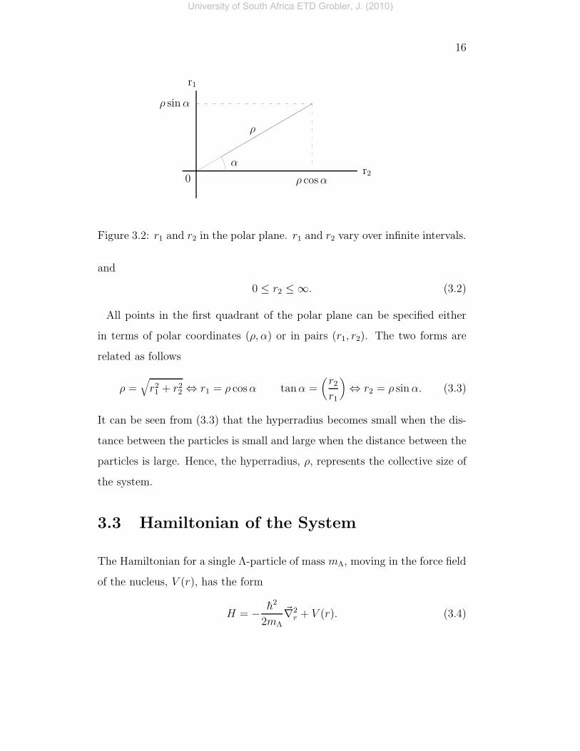
In Figure 3.2 the variables r1 and r2 vary over the infinite intervals

0 ≤ r1 ≤ ∞, (3.1)


16

α

ρ

0 ρ cosα

ρ sinα

r2

r1

Figure 3.2: r1 and r2 in the polar plane. r1 and r2 vary over infinite intervals.

and

0 ≤ r2 ≤ ∞. (3.2)

All points in the first quadrant of the polar plane can be specified either

in terms of polar coordinates (ρ, α) or in pairs (r1, r2). The two forms are

related as follows

ρ =√

r21 + r2

2 ⇔ r1 = ρ cosα tanα =(

r2r1

)

⇔ r2 = ρ sinα. (3.3)

It can be seen from (3.3) that the hyperradius becomes small when the dis-

tance between the particles is small and large when the distance between the

particles is large. Hence, the hyperradius, ρ, represents the collective size of

the system.

3.3 Hamiltonian of the System

The Hamiltonian for a single Λ-particle of mass mΛ, moving in the force field

of the nucleus, V (r), has the form

H = − h2

2mΛ

~∇2r + V (r). (3.4)


17

The potential, V (r), is rotationally invariant, depending only on the distance

r from the centre of force, which is chosen to be the centre of the nucleus.

Hence, the potential V (r) is a central potential. As we have assumed a

central potential, the wave function can be factored into both radial and

angular parts.

The Hamiltonian (3.4) is easily extended for the case of two Λ-particles,

H = − h2

2mΛ

(

~∇2~r1

+ ~∇2~r2

)

+[

VΛΛ(| ~r1 − ~r2 |) + V1(r1) + V2(r2)]

, (3.5)

where

VΛΛ(| ~r1 − ~r2 |) (3.6)

is the interaction potential between the two Λ-particles; −h2~∇2~r1/2mΛ and

−h2~∇2~r2/2mΛ are the kinetic energy operators for Λ-particles 1 and 2, respec-

tively; and V1(r1) and V2(r2) are the interaction potentials for each of the

two Λ-particles with the nucleus.

For the sake of convenience, we recast the Hamiltonian (3.5) in terms of

hypersperical coordinates, considering each term on the right-hand side of

(3.5) individually. We begin with the operator ~∇2~r in (3.5).

The operator ~∇2~r, can be written in spherical coordinates as

~∇2r =

1

r2

∂

∂r

(

r2 ∂

∂r

)

−~ℓ2

r2. (3.7)

Subsituting (3.7) into the term(

~∇2~r1

+ ~∇2~r2

)

, we obtain

(

~∇2~r1

+ ~∇2~r2

)

=1

r21

∂

∂r1

(

r21

∂

∂r1

)

+1

r22

∂

∂r2

(

r22

∂

∂r2

)

−~ℓ2~r1

r21

−~ℓ2~r2

r22

, (3.8)

where the angular momentum operators ~ℓ2~r1and ~ℓ2~r2

satisfy the normalized

eigenfunction equations of spherical harmonics

~ℓ2~r1= Yℓ1m1 = ℓ1(ℓ1 + 1)Yℓ1m1 , (3.9)


18

and

~ℓ2~r2= Yℓ2m2 = ℓ2(ℓ2 + 1)Yℓ2m2 . (3.10)

The total angular momentum of the system is conserved and is a constant

of the motion. Noting also that

1

r2

∂

∂r

(

r2 ∂

∂r

)

=∂2

∂r2+

2

r

∂

∂r, (3.11)

and substituting (3.11) into (3.8), we obtain

(

~∇2~r1

+ ~∇2~r2

)

=(

∂2

∂r21

+∂2

∂r22

)

+ 2(

1

r1

∂

∂r1+

1

r2

∂

∂r2

)

−~ℓ2~r1

r21

−~ℓ2~r2

r22

. (3.12)

The first term on the right hand side of (3.12) is a two-dimensional Laplacian

which can be written in terms of polar coordinates as

(

∂2

∂r21

+∂2

∂r22

)

=1

ρ

∂

∂ρ

(

ρ∂

∂ρ

)

+1

ρ2

∂2

∂α2, (3.13)

and the second term on the right hand side of (3.12) can also be written in

terms of polar coordinates as

(

1

r1

∂

∂r1+

1

r2

∂

∂r2

)

=(

∂ρ

∂r1

∂

∂ρ

)

+(

∂α

∂r1

∂

∂α

)

+(

∂ρ

∂r2

∂

∂ρ

)

+(

∂α

∂r2

∂

∂α

)

. (3.14)

The individual terms on the right hand side of (3.14) can be written as,

∂ρ

∂r1=

∂

∂r1

(

√

r21 + r2

2

)

=1

2

(

r21 + r2

2

)12−1 ∂

∂r1(r2

1) = cosα, (3.15)

∂α

∂r1=

∂

∂r1

[

arctan(

r2r1

)

]

= − r2r21 + r2

2

= −1

ρsinα, (3.16)

∂ρ

∂r2=

∂

∂r2

(

√

r21 + r2

2

)

=1

2

(

r21 + r2

2

)12−1 ∂

∂r1(r2

2) = sinα, (3.17)

and∂α

∂r2=

∂

∂r2

[

arctan(

r2r1

)

]

=r1

r21 + r2

2

=1

ρcosα. (3.18)


19

Substituting (3.15) to (3.18) into (3.14), we obtain

(

1

r1

∂

∂r1+

1

r2

∂

∂r2

)

=1

r1

(

cosα∂

∂ρ− 1

ρsinα

∂

∂α

)

+1

r2

(

sinα∂

∂ρ+

1

ρcosα

∂

∂α

)

=1

ρ

∂

∂ρ− 1

ρ2tanα

∂

∂ρ+

1

ρ

∂

∂ρ+

1

ρ2cotα

∂

∂α

=2

ρ

∂

∂ρ+

1

ρ2( cotα− tanα)

∂

∂α.

Since,

cotα− tanα = 2 cot 2α,

hence, the second term on the right hand side of (3.12) becomes

2(

1

r1

∂

∂r1+

1

r2

∂

∂r2

)

=4

ρ

∂

∂ρ+

4

ρ2cot 2α

∂

∂α. (3.19)

The first term on the right hand side of (3.13) can be written as

1

ρ

∂

∂ρ

(

ρ∂

∂ρ

)

=1

ρ

(

∂

∂ρ

∂

∂ρρ)

+ ρ(

∂

∂ρ

∂

∂ρ

)

=1

ρ

∂

∂ρ+

∂2

∂ρ2. (3.20)

Substituting (3.13), (3.19) and (3.20) into (3.12), we obtain

(

~∇2~r1

+ ~∇2~r2

)

=1

ρ

∂

∂ρ+

∂2

∂ρ2+

1

ρ2

∂2

∂α2+

4

ρ

∂

∂ρ+

4

ρ2cot 2α

∂

∂α

−~ℓ2~r1

ρ2 cos2 α−

~ℓ2~r2

ρ2 sin2 α

=∂2

∂ρ2+

5

ρ

∂

∂ρ− 1

ρ2

(

− ∂2

∂α2− 4 cot 2α

∂

∂α

−~ℓ2~r1

cos2 α−

~ℓ2~r2

sin2 α

)

=∂2

∂ρ2+

5

ρ

∂

∂ρ− 1

ρ2K2, (3.21)


20

where,

K2 =(

− ∂2

∂α2− 4 cot (2α)

∂

∂α+

~ℓ2~r1

cos2 α+

~ℓ2~r2

sin2 α

)

. (3.22)

The operator K2, and the associated eigenfunctions, are covered in the theory

of hyperspherical harmonics [25]. The operator K2 absorbs all the angular

variables. The solutions of the eigenvalue problem

K2φ[L](ω) = L(L+ 4)φ[L](ω), (3.23)

are the so-called hyperspherical harmonics which depend on the set of hy-

perangles

ω = Ω~r1,Ω~r2 , α.

The subscript [L] in (3.23) is the multi-index

[L] = L, ℓ1, ℓ2, m1, m2, (3.24)

which includes the grand orbital quantum number,

L = ℓ1 + ℓ2 + 2n, n = 0, 1, 2 . . . . (3.25)

The function φ[L](ω) introduced in (3.23) is of the form

φ[L](ω) = Kℓ1ℓ2m1m2L (ω)χ[s], (3.26)

where, the factor

Kℓ1ℓ2m1m2L (ω) = N ℓ1ℓ2

L (cosα)ℓ1(sinα)ℓ2P ℓ2+12,ℓ1+

12 (cos 2α)Yℓ1m1Yℓ2m2 , (3.27)

contains the hyperangular components [19].

The factor χ[s] is the three-body spin state vector, with [s] = ((s1s2)s12s3)sσ.

Subscripts 1, 2 and 3 represent the spins of the two Λ-particles and the nu-

cleus, respectively. The term s represents the three-body spin and P ℓ2+12,ℓ1+

12


21

is the spin permutation operator (also written in the form P σ), which acts

in the spin space.

The factor N ℓ1ℓ2L has the form

N ℓ1ℓ2L =

√

√

√

√

2n!(L+ 2)(n+ ℓ1 + ℓ2 + 1)!

Γ(n+ ℓ1 + 32)Γ(n+ ℓ2 + 3

2). (3.28)

Substituting (3.21) into (3.5), we obtain

H = − h2

2mΛ

(

∂2

∂ρ2+

5

ρ

∂

∂ρ− 1

ρ2K2)

+ VΛΛ(| ~r1 − ~r2 |) + V1(r1) + V2(r2)

= Ho + VΛΛ(| ~r1 − ~r2 |) + V1(r1) + V2(r2),

where

Ho = − h2

2mΛ

(

∂2

∂ρ2+

5

ρ

∂

∂ρ− 1

ρ2K2)

. (3.29)

Hence, the Hamiltonian for the system is

H = Ho + VΛΛ + V1 + V2, (3.30)

where Ho is of the form (3.29).

3.3.1 Volume Element

The volume element in the hyperspherical coordinate system is

d~r1 d~r2 = r21r

22 sin θ~r1 sin θ~r2 dr1 dr2 dθ~r1 dθ~r2 dϕ~r1 dϕ~r2. (3.31)

In polar coordinates, we have

dr1 dr2 = ρ dρ dα, (3.32)

and substituting (3.3) and (3.32) into (3.31), we obtain

d~r1 d~r2 = (ρ2 cos2 α)(ρ2 sin2 α) sin θ~r1 sin θ~r2ρ dρ dα dθ~r1 dθ~r2 dϕ~r1 dϕ~r2


22

= (ρ5dρ)( sin2 α cos2 αρ2dα)( sin θ~r1dθ~r1dϕ~r1)( sin θ~r2 dθ~r2 dϕ~r2)

= (ρ5 dρ)( sin2 α cos2 αρ2 dα) dΩ~r1 dΩ~r2

= ρ5 dρ dω,

where

dω =1

4sin2 2α dα dΩ~r1 dΩ~r1, (3.33)

and

dΩ~r1 = sin θ~r1 dθ~r1 dϕ~r2,

which is defined as the spherical angle. Integrating (3.33) over the interval

0 ≤ α ≤ π/2, we obtain the volume element in the hyperspherical coordinate

system,

∫ π

2

0dω =

∫ π

2

0

1

4sin2 α dα dΩ~r1 dΩ~r2

=∫ π

2

0

1

4sin2 α dα

(

∫ π

0sin θ~r1 dθ~r1

∫ 2π

0dϕ~r1

)(

∫ π

0sin θ~r2dθ~r2

∫ 2π

0dϕ~r2

)

= 16π2∫ π

2

0

1

4sin2 α dα

= 16π2

(

1

8

∫ π

2

0dα− 1

2

∫ π

2

0cos 4α dα

)

= 16π2(

π

16

)

= π3. (3.34)


23

3.4 Schrodinger Equation of the System

The central-force problem proposed in our system enables the reduction of

the six-dimensional Schrodinger Equation of the form

Hψ(~r1, ~r2) = Eψ(~r1, ~r2). (3.35)

In order to derive the Schrodinger Equation for the system, we use an ap-

proach similar to the two-body partial wave decomposition [25], where a

two-body wave function of the form

ψ(~r1, ~r2) =1

ρ52

∑

[L]

u[L](ρ)φ[L](ω), (3.36)

is employed and the hyperradial and angular components are included in the

terms u[L] and φ[L](ω), respectively. The coefficient 1/ρ52 is introduced in

order to eliminate the first-order derivative in the hyperradial Schrodinger

Equation. The hyperangle, ω, is related to the pair (~r1, ~r2).

Substituting (3.30) and (3.36) into (3.35), we obtain for the first term

[

− h2

2mΛ

(

∂2

∂ρ2+

5

ρ

∂

∂ρ− 1

ρ2K2

)

+ VΛΛ(| ~r1 − ~r2 |) + V1(r1) + V2(r2)

]

×(

1

ρ52

∑

[L]

u[L](ρ)φ[L](ω)

)

= E

(

1

ρ52

∑

[L]

u[L](ρ)φ[L](ω)

)

.(3.37)

Evaluating the first two terms in parenthesis on the left-hand side of (3.37),

we obtain, for the first term

∂2

∂ρ2

(

1

ρ52

∑

[L]

u[L](ρ)φ[L](ω)

)

=∂

∂ρ

[

∂

∂ρ

(

1

ρ52

∑

[L]

u[L](ρ)φ[L](ω)

)]

=∂

∂ρ

[(

∑

[L]

u[L](ρ)φ[L](ω)

)

∂

∂ρ

(

1

ρ52

)

+1

ρ52

∂

∂ρ

(

∑

[L]

u[L](ρ)φ[L](ω)

)]


24

=∂

∂ρ

[

− 5

2ρ72

(

∑

[L]

u[L](ρ)φ[L](ω)

)

+1

ρ52

(

∑

[L]

u′[L](ρ)φ[L](ω)

)]

=35

4ρ92

(

∑

[L]

u[L](ρ)φ[L](ω)

)

− 5

2ρ72

(

∑

[L]


)

− 5

2ρ72

(

∑

[L]


)

+1

ρ52

(

∑

[L]

u′′[L](ρ)φ[L](ω)

)

, (3.38)

and, for the second term

5

ρ

∂

∂ρ

(

1

ρ52

∑

[L]

u[L](ρ)φ[L](ω)

)

=

[

5

ρ

(

∑

[L]

u[L](ρ)φ[L](ω)

)

∂

∂ρ

(

1

∂52

)]

+

[

5

ρ

1

ρ52

∂

∂ρ

(

∑

[L]

u[L](ρ)φ[L](ω)

)]

= − 25

9ρ92

(

∑

[L]

u[L](ρ)φ[L](ω)

)

+5

ρ72

(

∑

[L]


)

. (3.39)

Substituting (3.38) and (3.39) into (3.29), we obtain,

Hoψ(~r1~r2) = − h2

2mΛ

(

∂2

∂ρ2+

5

ρ

∂

∂ρ− 1

ρ2K2

)(

1

ρ52

∑

[L]

u[L](ρ)φ[L](ω)

)

= − h2

2mΛ

[(

35

4ρ92

∑

[L]

u[L](ρ)φ[L](ω)

)

+1

ρ52

(

∑

[L]

u′′[L](ρ)φ[L](ω)

)

− 1

ρ52

(

∑

[L]

u[L](ρ)φ[L](ω)

)

− 1

∂2

1

ρ52

K2

(

∑

[L]

u[L](ρ)φ[L](ω)

)]

= − h2

2mΛ

∑

[L]

u[L]

[

35

4ρ92

u[L](ρ)φ[L](ω) +1

ρ52

u′′[L](ρ)φ[L](ω) −

25

2ρ92

u[L](ρ)φ[L](ω) − 1

2ρ92

u[L]L(L+ 4)(ρ)φ[L](ω)

]

= − h2

2mΛ

∑

[L]

[

1

ρ52

u[L](ρ)φ[L](ω) +15

2ρ92

u[L](ρ)φ[L](ω) −


25

1

ρ92

u[L]L(L+ 4)(ρ)φ[L](ω)

]

= − h2

2mΛ

∑

[L]

[

1

ρ52

u′′[L](ρ)φ[L](ω) −(

L(L+ 4) + 154

ρ92

)

u[L](ρ)

]

φ[L](ω).(3.40)

Substituting (3.40) into (3.37), we obtain the following eigenvalue equation

Hψ(~r1, ~r2) = − h2

2mΛ

∑

[L]

[

1

ρ52

u′′[L](ρ)φ[L](ω) −(

L(L+ 4) + 154

ρ92

)

u[L](ρ)

]

φ[L](ω)

=

[

VΛΛ(| ~r1 − ~r2 |) + V1(r1) + V2(r2)

]

1

ρ52

∑

[L]

u[L](ρ)φ[L](ω)

= E1

ρ52

∑

[L]

u[L](ρ)φ[L](ω). (3.41)

Next, we multiply (3.41) on the left-hand side by

−2mΛ

h2 ρ52φ∗

[L](ω),

(“∗” represents the complex conjugate) and then integrate with respect to ω

over all the angular variables, giving

− h2

2mΛ

2mΛρ52

h2

∫

∑

[L]

[

1

ρ52

u′′[L](ρ)φ[L](ω) −(

L(L+ 4) + 154

ρ92

)

u[L](ρ)

]

φ∗[L](ω)φ[L′](ω) dω

+2mΛρ

52]

h2

1

ρ52

∫

[

VΛΛ(| ~r1 − ~r2 |) + V1(r1) + V2(r2)

]

∑

[L]

u[L](ρ)φ∗[L](ω)φ[L′](ω)dω

= E2mΛρ

52

h2

[

1

ρ52

∫

∑

[L]

u[L](ρ)φ∗[L](ω)φ[L′](ω) dω

]

[

u′′[L](ρ) −(

L(L+ 4) + 154

ρ2

)]

u[L](ρ) +∑

[L]

2mΛ

h2

[

∫

(VΛΛ(| ~r1 − ~r2 |) + V1(r1) + V2(r2))

×φ∗[L](ω)φ[L′](ω) dω

]

u[L′](ρ) =2mΛE

h2 u[L](ρ).


26

Hence, we obtain the following system of hyperradial equations[

∂2

∂ρ2+ k2 − L(L+ 4) + 15

4

ρ2

]

u[L](ρ) =∑

[L]

V[L][L′](ρ)u[L′](ρ), (3.42)

where V[L][L′] is a potential matrix of the form

V[L][L′] =2mΛ

h2

∫

φ∗[L](ω)

[

VΛΛ(| ~r1 − ~r2 |) + V1(r1) + V2(r2)]

φ[L′](ω) dω.

Introducing the parameter λ and substituting this into (3.42), where

λ = L+3

2, (3.43)

and noting that

L(L+ 4) +15

4=

(

L+3

2

)(

L+5

2

)

= λ(λ+ 1),

we obtain the desired result, the set of hyperradial Schrodinger Equations

for the system[

∂2

∂ρ2+ k2 − λ(λ+ 1)

ρ2

]

u[L](k, ρ) =∑

[L′]

V[L][L′](ρ)u[L′](k, ρ), (3.44)

where k, the hypermomentum, is given by

k2 =2mΛE

h2 ,

where use has been made of the orthonormality relation of hyperspherical

harmonics

∫

φ∗[L](ω)φ[L′](ω)dω = δ[L]δ[L′],

and the relation [21]

χ†[s]χ[s] = 1.


Chapter 4

Method of Solution

4.1 The Jost Function

We consider the general form of the radial Schrodinger Equation [21]

[

∂2

∂r2+ k2 − l(l + 1)

r2− V (r)

]

ul(k, r) = 0, (4.1)

where k2 = 2mE/h2, l is the angular momentum quantum number, ul(k, r)

is the radial wave function, and r is the radius.

The boundary conditions for the physical solutions of (4.1) are imposed at

both ends of the interval r ∈ [0,∞). Regularity of the wave function at the

origin requires that

ul(k, 0) = 0, (4.2)

a condition which exists for all solutions. However, the conditions for r → ∞are different for bound, scattering and resonant states. If the potential V (r)

vanishes at large distances faster than 1/r2, then (4.1) takes the form of the

“free” radial Schrodinger Equation [26],

[

∂2

∂r2+ k2 − l(l + 1)

r2

]

ul(k, r) = 0. (4.3)

27


28

This equation has two linearly independent solutions, namely, the Riccati-

Hankel functions h(−)l (kr) and h

(+)l (kr) [27], which behave as

h(±)l (kr) −→

r→∞∓i exp[±i(kr − lπ/2)]. (4.4)

The general asymptotic form of the wavefunction can be constructed from a

linear combination of these Riccati-Hankel functions,

ul(k, r) −→r→∞

C1h(−)l (kr) + C2h

(+)l (kr), (4.5)

where appropriate choice of the combination coefficients C1 and C2 determine

the type of physical solutions. These coefficients are functions of the total

energy of the system and the angular momentum. The radial wavefunction

ul(k, r) can be written in terms of the asymptotics of (4.4) as

ul(k, r) −→r→∞

h(−)l (kr)f

(−)l (k) + h

(+)l (kr)f

(+)l (k), (4.6)

where C1 = f(−)l (k) and C2 = f

(+)l (k). The energy-dependent amplitudes

f(±)l (k) of the incoming and outgoing waves are called the Jost functions [26].

For bound states, the wave function (4.6) must vanish at large distances

ul(kn, r) −→r→∞

0. (4.7)

The total energy for a bound state is negative and the momentum is pure

imaginary

kn =√

−2m|En|/h2 = iκn, κn > 0. (4.8)

Substituting (4.8) into (4.4), we find that one of the two asymptotic terms

of (4.4) grows exponentially, while the other vanishes exponentially

h(±)l (kr) ∼

r→∞exp (∓κr). (4.9)


29

Therefore, only the second term in (4.6) can survive in the bound state wave

function,

ul(kn, r) −→r→∞

h(+)l (knr)f

(+)l (kn). (4.10)

This may be achieved for certain points such that

f(−)l (kn) = 0. (4.11)

Therefore, bound states correspond to positive imaginary zeros of the Jost

function.

The Jost function is a complex function of the total energy of the quantum

state, which may be real or complex. The most useful property of the Jost

function is that it is an analytic function for all complex energies and has

simple zeros for bound states. It seems therefore logical to approach a solu-

tion to our model by using a method to determine the Jost function as we

could then determine the bound states.

4.2 Three-body Jost Matrix

The Jost function for the single-channel case were covered in the previous

section. As our hypernuclear system is a three-body problem, we recast the

formalism of the previous section for the multi-channel case.

A method for calculating the Jost function for analytic potential were de-

veloped, and successfully applied to hypernuclear systems [19, 28, 29]. The

method uses a combination of the hyperspherical approach, complex rotation

and the properties of the Jost function in order to determine bound states.


30

The physical solutions of (3.44) are defined by the boundary condition re-

quirement

u[L](k, ρ)−→ρ→0

0, (4.12)

and, at infinity must be of the form

u[L](k, ρ) −→ρ→∞

U[L](k, ρ), (4.13)

where U[L](k, ρ) has terms describing the open channels.

We follow the methods set out in [19, 28, 29] and consider (3.44) as a matrix

equation with each of its solutions forming a column matrix. According to

the general theory of differential equations, there are as many independent

regular column-solutions as there are equations in the system [30],[

∂2

∂ρ2+ k2 − λ(λ+ 1)

ρ2

]

Φ[L][L′](k, ρ) =∑

[L′′]

V[L][L′′](ρ)Φ[L][L′′](k, ρ), (4.14)

where

Φ[L][L′](k, ρ) =1

2

[

h(−)λ (kρ)F

(−)[L][L′](k, ρ) + h

(+)λ (kρ)F

(+)[L][L′](k, ρ)

]

, (4.15)

and h(±)λ (kρ) are the Riccati-Hankel functions [27]. The inclusion of the

Riccati-Hankel in the construction of the regular basis ensures the correct

asymptotic behaviour of the basic solutions at large ρ.

The two terms ||F (±)[L][L′](k, ρ)|| in (4.15) are unknown matrices, introduced in

order for the construction of different physical solutions. Since according to

(4.12), all physical solutions must be regular at ρ = 0, any one of them is a

linear combination of the regular column-solutions. As we seek to determine

these two unknown matrices, reason dictates [30] that we need two equations.

We obtain these equations by making use of the Lagrange condition

h(−)λ (kρ)F

(−)[L][L′](k, ρ) + h

(+)λ (kρ)F

(+)[L][L′](k, ρ) = 0. (4.16)


31

Substituting (4.15) into the hyperradial equation (4.14) and using the condi-

tion (4.16), we obtain the following system of first-order coupled differential

equations for the unknown matrices F(±)[L][L′](k, ρ),

∂ρF(−)[L][L′](k, ρ) = −h

(+)λ (kρ)

2ik

∑

[L′′]

V[L][L′′](ρ)[

h(−)λ′′ (kρ)F

(−)[L′′][L′](k, ρ),

+h(+)λ (kρ)F

(+)[L′′][L](k, ρ)

]

,

∂ρF(+)[L][L′](k, ρ) =

h(−)λ (kρ)

2ik

∑

[L′′]

V[L][L′′](ρ)[

h(−)λ′′ (kρ)F

(−)[L′′][L′](k, ρ),

+h(+)λ (kρ)F

(+)[L′′][L](k, ρ)

]

,

(4.17)

which are equivalent to (3.44). These equations are convenient for solving

our model.

The equations (4.17) require suitable boundary conditions at ρ = 0. It

can be shown [31] that for a three-body system, the coupled hyperradial

Schrodinger Equations (4.17) have a system of linearly independent, regular

column solutions which vanish near ρ = 0 such that

limρ→0

Φ[L][L′](k, ρ)

ρλ′+1= δ[L][L′]. (4.18)

To ensure consistency with the definition of the regular solution, we define a

regular basis using the boundary condition [31]

limρ→0

Φ[L][L′](k, ρ)

jλ′(kρ)= δ[L][L′], (4.19)

where jλ′(kρ) is the Riccati-Bessel function [27], in accordance with the cor-

responding definition of the three-body problem.

As Φ[L][L′](k, ρ) is regular at ρ = 0, we can expect that the functions F(±)[L][L′](k, ρ)

of (4.15) near the origin ensure that the singularities of h(±)λ (kρ) compensate


32

each other. Such a condition is achieved [31] if the functions F(±)[L][L′](kρ) are

identical as ρ→ 0, or

F(±)[L][L′](k, ρ) ∼

ρ→0F[L][L′](k, ρ), (4.20)

as then

Φ[L][L′](k, ρ) ∼ρ→0

jλ(kρ)F[L][L′](k, ρ), (4.21)

so that the boundary conditions (4.19) then become

limρ→0

[

jλ(kρ)F[L][L′](k, ρ)

jλ′(kρ)

]

= δ[L][L′]. (4.22)

However, ρ = 0 is a singular point as the Riccati-Hankel functions have

the short-range behaviour ≈ ρ−L. Therefore, Eqs. (4.17) cannot be solved

numerically with the boundary conditions at ρ = 0. We may [29], however,

use analytical solutions (in the form of a series expansion) of (4.17) in the

small interval (0, δ], imposing the boundary conditions at ρ = δ

F(±)[L][L′](k, δ) ≈ F

(N)[L][L′](k, δ). (4.23)

The right hand side of (4.17) vanishes when ρ → ∞ [31]. The derivatives of

(4.17) also vanish, therefore the functions F(±)[L][L′](k, ρ) become ρ-independent.

Hence, we have

Φ[L][L′](k, ρ) ∼ρ→∞

1

2

[

h(−)λ (kρ)f

(−)[L][L′](k) + h

(+)λ (kρ)f

(+)[L][L′](k)

]

, (4.24)

where

f(±)[L][L′](k) = lim

ρ→∞F

(±)[L][L′](k, ρ). (4.25)

There ρ-independent matrices ||f (±)[L][L′]|| are termed the Jost matrices.

The Jost matrices can be used to determine the asymptotic behaviour of the

fundamental system of regular solutions (4.17).


33

For complex values of k, the limits (4.25) exist in different domains of the

complex plane, namely, f(+)[L][L′](k) in the lower half and f

(−)[L][L′](k) in the upper

half. For a particular class of potentials, the upper bound for the existence

of f(+)[L][L′](k) is shifted upwards and the lower bound for f

(−)[L][L′](k) is shifted

downwards, thereby widening their common area. Difficulties concerning

the existence of the limits (4.25) can be circumvented by using the complex

rotation method which is discussed in the sections that follow.

4.3 Method of Locating Bound States

In the theory of quantum mechanics [32], a bound state is characterized by

wave functions which vanish at large distances. This is because the proba-

bility of locating a bound particle at large distances from the bound region

must decrease with increasing distance from that region. The probability is

directly dependent on the modulus of the wave function,

ψ(r) −→ρ→∞

0.

The deuteron is an example of a bound state of the proton and the neutron.

The binding energy of the deuteron is 2.22 MeV and is the only bound state

of two nucleons [2]. The bound state of the deuteron may exist indefinitely.

Bound states occur at negative energies, where the potentials describing such

behaviour are negative, thereby having a “pulling-in” effect. An example of

such a potential is the optical potential [21].

The bound state wave function, at large distances, can be written as

∑

[L′]

Φ[L][L′](k, ρ)C[L′] −→ρ→∞

0. (4.26)


34

Here, the function Φ[L][L′](k, ρ) can be replaced by its asymptotic form

1

2

∑

[L′]

[h(+)λ (kρ)f

(+)[L][L′](k) + h

(−)λ (kρ)f

(−)[L][L′](k)]C[L′] −→

ρ→∞0. (4.27)

The total energy for a bound state is negative with the corresponding mo-

mentum being pure imaginary. Due to the properties of the Riccati-Hankel

functions, with increasing distances from the origin, the term h(−)λ (kρ) of

(4.27) grows exponentially while the other term h(+)λ (kρ) decays exponen-

tially. Hence, the condition (4.27) can only be achieved if we find combina-

tion coefficients C[L′] such that the diverging functions h(−)λ (kρ) of different

columns cancel out, giving

∑

[L′]

f(−)[L][L′](k)C[L′] = 0. (4.28)

Bound states are the points at which the physical solution consists of only

outgoing waves in its asymptotics.

The system of homogenous linear equations has a non-trivial solution pro-

vided that

det ||f (−)(k)|| = 0. (4.29)

The condition (4.29) enables us to determine all possible bound states by

looking for zeros of the Jost matrix determinant on the positive imaginary

axis. For each zero found, the coefficients C[L] are then uniquely determined

by the system (4.28) apart from a general normalization factor. The normal-

ization factor is fixed when the physical wavefunction is normalized.

4.4 Minimal Approximation

The Schrodinger Equation (3.44) is of the same form as the radial coupled-

channels Schrodinger equation [32] and includes the centrifugal potential


35

term λ(λ+ 1)/ρ2. These similarities enable the Schrodinger Equation (3.44)

to be solved using the Jost function method [19, 28, 29].

However, the system (3.44) consists of an infinite number of equations and

in order to make it of any practical use, we have to truncate it somewhere.

In order to achieve this, we employ the minimal approximation method.

In the minimal approximation we retain only the first term in (3.36), giving

ψ(~r1, ~r2) ≈1

ρ52

u[Lmin](ρ)φ[Lmin](ω),

and we assume the minimal value of the grand orbital angular momentum,

n = 0, called the hypercentral approximation. In this approximation, (3.24)

becomes [L] = [Lmin], with L = Lmin = 0, giving

λ = λmin =3

2,

and

[

∂2

∂ρ2+ k2 − λmin(λmin + 1)

ρ2

]

u[0](k, ρ) = 〈U〉u[0](k, ρ),

where

〈U〉 =2mΛ

h2

∫

φ∗[0](ω)

[

VΛΛ(| ~r1 − ~r2 |) + V1(r1) + V2(r2)]

φ[0](ω)dω. (4.30)

For the case ℓ1 = ℓ2 = Lmin = 0, we have

N000 =

4√π, (4.31)

P12

12 = 1, (4.32)

and,

K00000 = π−3/2. (4.33)


36

Hence, (3.26) takes the form

φ[0] = π− 32 . (4.34)

Substituting (4.34) into (4.30), we obtain the hypercentral potential for our

hypernuclear system

〈U〉 =2mΛ

π3h2

∫

[

VΛΛ(| ~r1 − ~r2 |) + V1(r1) + V2(r2)]

dω. (4.35)

The first term of (4.35), VΛΛ(| ~r1 − ~r2 |), represents the two-body potential

acting between the two Λ-particles. The terms V1(r1) and V2(r2) represent

the interaction between each of the two Λ-particles and the nucleus.

In order to use (4.35), we first need to obtain suitable forms for VΛΛ(| ~r1−~r2 |),V1(r1) and V2(r2). Suitable forms for these are discussed in the sections that

follow.

We see from (4.35) that the hypercentral potential has the general form

〈U〉 = 〈V12〉 + 〈V13〉 + 〈V23〉, (4.36)

where 〈V12〉 represents the two-body potential acting between the two iden-

tical Λ-particles. The terms 〈V13〉 and 〈V23〉 represent the potential acting

between each of the two Λ-particles and the nucleus.

Applying the minimal approximation to (3.44) and (4.17), we end up with a

single pair of equations,

∂ρF(−)[Lmin][L′

min](k, ρ) = −h

(+)λ (kρ)

2ik〈U〉

[

h(−)λ′′ (kρ)F

(−)[L′′

min][L′

min](k, ρ),

+h(+)λ F

(+)[L′′

min][L′

min](k, ρ)

]

,

∂ρF(+)[Lmin][L′

min](k, ρ) =

h(−)λ (kρ)

2ik〈U〉

[

h(−)λ′′ (kρ)F

(−)[L′′

min][L′

min](k, ρ),

+h(+)λ (kρ)F

(+)[L′′

min][L′

min](k, ρ)

]

(4.37)


37

The set of equations (4.37) form the crux of our model.

4.5 ΛΛ-Potential

In our model, we need a two-body potential which describes the interaction

between the two Λ-particles. A suitable form for such a potential is (4.38).

This potential has been successfully used in few-body calculations [11]. The

potential (4.38) represents a weak attraction, having the three-range Gaus-

sian form

VΛΛ(ρ) =3∑

i=1

Ai exp ( − ρ2/β2i ), (4.38)

and describes the S-wave interaction of two Λ-particles with the total spin

being zero, an S-state. The ΛΛ-potential provides a means of simulating

the effect of ΛΛ → ΞN coupling of the baryon-baryon interaction through

modification of the strength of the relevant part of the potential.

The parameters of this potential are listed in Table 4.1.

i Ai [MeV] βi [fm]

1 -21.49 1.342

2 -379.1 ×γ 0.777

3 9324 0.350

Table 4.1: Parameters of the ΛΛ-potential. The strength of the long-rangepart of the potential is reduced by multipliying by the factor γ = 0.6598 inorder to ensure agreement with experimental results [11].

The ΛΛ-potential of the type (4.38) is shown in Figure 4.1 for real ρ.

In order to use (4.38), we must ensure that this potential is an analytic func-

tion of ρ. This condition enables the potential to be analytically continued


38

-1000

0

1000

2000

3000

4000

5000

6000

7000

8000

9000

10000

0 0.2 0.4 0.6 0.8 1

VΛ

Λ(M

eV)

Radius (fm)

Figure 4.1: ΛΛ-potential. The potential decays exponentially, approaches anegligible value at about 0.7 fm.

from the real axis into the complex ρ-plane. Fortunately, in most cases the

model potential has an analytic tail at large distances. In our case the poten-

tial is continuous everywhere. For our purposes, it is sufficient to show that

(4.38) is an analytic function of ρ by using the following two conditions [28],

limρ→0

ρ2V (ρ) = 0,

and

limρ→0

ρV (ρ) = 0.

For the first condition we have

limρ→0

ρ2VΛΛ(ρ) = limρ→0

ρ2[

A1 exp ( − ρ2/β21) + A2 exp ( − ρ2/β2

2) + A3 exp ( − ρ2/β23)]

= 0

and, for the second


39

limρ→∞

ρVΛΛ(ρ) = limρ→∞

ρ[

A1 exp ( − ρ2/β21) + A2 exp ( − ρ2/β2

2) + A3 exp ( − ρ2/β23)]

= 0.

Hence, the ΛΛ-potential is less singular at the origin than the centrifugal

term, vanishes at infinity faster than the Coulomb potential, and is an ana-

lytic function of ρ. Therefore, the potential (4.38) is suitable for our purposes.

4.6 Λ-Nucleus Potential

The Woods-Saxon potential with a well depth of about 30 MeV is seen to de-

scribe various orbital angular momentum binding energies for data obtained

in emulsion studies [24]. The low momentum transfer reaction,(K−,π−),

studied with various targets is described reasonably well using the Woods-

Saxon potential with a well depth of about 30 MeV. The depth of 30 MeV has

been determined from the asymptotic binding energy of the lowest orbital

angular momentum for large A. The nuclear medium density is characterized

by a Fermi distribution of the form 1 + exp[

(r − c)/a]

.

In (4.35) we use, for V1(r1) and V2(r2), a Λ-nucleus potential of the Woods-

Saxon type (4.39), with a well depth in the region of 30 MeV and which

decreases with increasing mass number,

VΛ1(r1) = − W

1 + exp [(r1 − c)/a], (4.39)

where,

c = ro(A)A13 . (4.40)

It has been shown that a potential of the form (4.35), with a well depth

of W = −28.0 MeV, radius parameter ro = (1.128 + 0.439A− 23 ) fm, and


40

diffusivity a = 0.6 fm, yields a reasonable description of Λ-nucleus single-

particle state binding energies [24]. Slightly different values may be used for

r1 and c, but these results are not very sensitive to small variations in these

parameters. The Λ-nucleus potential of the type (4.39) is shown in Figure

4.2.

-30

-25

-20

-15

-10

-5

0

0 1 2 3 4 5 6

V(M

eV)

Radius (fm)

Figure 4.2: Λ-nucleus potential for a well depth of W = −28.0 MeV, massnumber of A = 15 and diffusivity a = 0.6 fm. The potential falls off quiterapidly beyond the hypernuclear surface and approaches a negligibly smallvalue at ≈ 5 fm.


41

The Wood-Saxon potential (4.39) is an analytic function of ρ. Its asymptotic

behaviour at short and long distances is

limr1→0

r21VΛ1(r1) = lim

r1→0

[

r21

W

1 + exp [(r1 − c)/a]

]

=0

1 + exp [(0 − c)/a]

= 0

and,

limr1→∞

r1VΛ1(r1) = limr1→∞

[

r1W

1 + exp [(r1 − c)/a]

]

= 0.

Therefore, the Λ-nucleus potential is less singular at the origin than the

centrifugal term, vanishes at infinity faster than the Coulomb potential, and

is an analytic function of ρ.

4.7 Total Potential

The total potential for the hypernucleur system is the sum of the Λ-Nucleus

potential (4.38) and the ΛΛ-potential (4.39). We therefore combine (4.38)

and (4.39) in the hypercentral potential (4.35).

We start with the first term of the intergrand on the right hand side of the

integral (4.35). This term can be re-written using (3.33),

∫

VΛΛ(| ~r1 − ~r2 |) dω =∫

VΛΛ(| ~r1 − ~r2 |)[

1

4sin2 2α dα

× dΩ~r1 dΩ~r1

]


42

=∫

VΛΛ(| ~r1 − ~r2 |)[

1

4sin2 2α dα

×( sin θ~r1dθ~r1dϕ~r1)( sin θ~r2 dθ~r2 dϕ~r2)

]

. (4.41)

The term | ~r1−~r2 | in the intergrand of (4.41) represents the physical distance

between the two Λ-particles. This term can be re-written as

| ~r1 − ~r2 | =√

r21 + r2

2 − 2r1r2 cos θ

=√

ρ2 − 2ρ2 cosα sinα cos θ

= ρ√

1 − sin (2α) cos θ. (4.42)

In order to simplify (4.41), we orient the system with respect to θ1, with

θ1 = θ,

θ = θ1 ⇒∫

1

4sin2 (2α)[ sin θ~r2 dθ~r2 dϕ~r2] dα = 2π2

∫

1

4sin2 2α, dα

and hence, (4.41) becomes∫

VΛΛ(| ~r1 − ~r2 |) dω = 2π2∫ π

2

0dα∫ π

0sin θ dθ VΛΛ

(

ρ√

1 − sin (2α) cos θ)

× sin2 2α. (4.43)

Using a change of variable, t = cos θ in (4.43), with

dt = − sin θdθ,

θ = 0 ⇒ t = 1,

θ = π ⇒ t = −1,

and∫ π

0sin θ dθ = −

∫ −1

1dt

=∫ 1

−1dt,


43

gives

∫

VΛΛ(| ~r1 − ~r2 |) dω = 2π2∫ π

2

0dα∫ 1

−1dt VΛΛ

(

ρ√

1 − sin (2α)t)

× sin2 2α. (4.44)

Now, considering the integral,

∫ 1

−1exp

[

− ρ2

β2(1 − sin 2α)t

]

dt = exp(

− ρ2

β2

)∫ 1

−1exp

(

ρ2 sin 2α

β2t)

dt,(4.45)

and evaluating the right-hand side of (4.45), we obtain

∫ 1

−1exp

[

− ρ2

β2(1 − sin 2α)t

]

dt =β2

ρ2 sin 2αexp

(−ρ2

β2

)

[

exp(

ρ2 sin 2α

β2t)

]1

−1

=β2

ρ2 sin 2αexp

(−ρ2

β2

)

[

exp(

ρ2 sin 2α

β2

)

− exp(

− ρ2 sin 2α

β2

)

]

. (4.46)

Comparing (4.38) with (4.46), we see that each term of (4.38) generates an

expression such as (4.46). Therefore, (4.41) may be written in terms of (4.46),

as follows

∫

VΛΛ(| ~r1 − ~r2 |) dω =2π2

ρ2 sin2 2α

∫ π

2

0

3∑

i=1

Aiβi

exp[

ρ2

β2i

(1 − sin 2α)]

− exp[

− ρ2

β2i

(1 + sin 2α)]

sin2 2α dα

= 2π2∫ π

2

0

3∑

i=1

Ai

(

β2i

ρ2

)

exp[

ρ2

β2i

(1 − sin 2α)]

− exp[

− ρ2

β2i

(1 + sin 2α)]

sin 2α dα. (4.47)

Using a change of variable, X = 2α in (4.47), with

dX = 2 dα,


44

α = 0 ⇒ X = 0,

α =π

2⇒ X = π,

and

∫ π

2

02α dα =

∫ π

0dX, (4.48)

gives

∫

VΛΛ(| ~r1 − ~r2 |) dω = π2∫ π

0

3∑

i=1

Ai

(

β2i

ρ2

)

exp[

− ρ2

β2i

(1 − sinX)]

− exp[

− ρ2

β2i

(1 + sinX)]

sinX dX. (4.49)

The second term of the intergral (4.35), which represents the Λ-nucleus po-

tential, may be written using (3.33) as

∫

VΛ1(r1) dω =∫

VΛ1(ρ cosα) dω

=∫

VΛ1(ρ cosα)[

1

4sin2 2α dα dΩ~r1 dΩ~r2

]

= 4π2∫ π

2

0VΛ1(ρ cosα) sin2 2α dα. (4.50)

Similarily, for the second Λ-particle

∫

VΛ2(r1) dω = 4π2∫ π

2

0VΛ2(ρ sinα) sin2 2α dα. (4.51)

Finally, combining (4.49), (4.50), and (4.51), we obtain the total potential of

the hypernuclear system

〈U〉 =4mΛ

πh2

∫ π

0

[

VΛ1

[

ρ cos(

X

2

)]

+ VΛ2

[

ρ sin(

X

2

)]

sin2X

+3∑

i=1

Ai

(

β2i

ρ2

)

exp[

− ρ2

β2i

(1 − sinX)]

− exp[

− ρ2

β2i

(1 + sinX)]

sinX

]

dX, (4.52)


45

where we have used a change of variable similar to (4.48) in (4.50) and (4.51).

A graphical presentation of the hypercentral potential (4.52) is shown in

Figure 4.3.

〈U〉(

MeV

)

Radius (fm)

-50

0

50

100

150

200

1 2 3 4 5 6 7

A=4 A=20

Figure 4.3: Hypercentral potentials for A = 4 − 20. The minimum values ofthe potentials for A = 4 and A = 20 are about 2.5 fm and 2.8 fm, respectively.Note the increase in depth, ≈ 17 MeV, with increasing mass number forA = 4−20. The minimum of the hypercentral potential for A = 20 is shiftedby ≈ 0.5 fm relative to that for A = 4. The curves for A = 5−19 lie betweenthe two curves for A = 4 and A = 20.

The hypercentral potentials (or hyperradial potentials), (4.52), are used as

input to the single pair of differential equations, (4.37), in order to determine

the two-body Jost functions.

4.8 Complex Rotation

In certain regions of the complex energy plane, limiting values of (4.25) are

not achieved when the coupled differential equations (4.37) are integrated


46

along the real axis. The inherent problem associated with solving the pair of

coupled first-order differential equations (4.37) when the potential extends

to infinity, is solved by using the complex rotation method [29, 28].

The potentials are analytic functions of the hyperradius, ρ, which is true

in many cases and implies that the wave function (4.15) is also an analytic

function of ρ. An important property of an analytic function of ρ is that it

is independent of the path taken between any two values. In our case, we

cannot integrate the differential equations (4.37) along the real axis. The

cruical step to solving this problem is to replace the real hyperradius ρ with

a complex hyperradius of the form (4.53). This enables integration of (4.37)

in the complex plane, along the path from 0 to ρ′ as depicted in Figure 4.4.

θ

0 ρ

ρ′

Re ρ

Im ρ

Figure 4.4: Deformed contour showing path of integration for (4.55) withcomplex energies.

We are concerned only with the asymptotic coefficients, f(−)[L][L′](k) and f

(+)[L][L′](k),

which are ρ-independent, and are the same for all points on the arc ρρ′.

Therefore, it is sufficient to solve the Schrodinger Equation from the point 0

to ρ′. The arc ρρ′ desribes rotation of the segment 0 to ρ′ on the real axis.


47

Complex rotation is expressed in terms of the hyperradius as follows

ρ = β exp (iθ), β ≥ 0, (4.53)

where the interval of the rotation angle θ is

0 < |θ| < π

2. (4.54)

Using a large enough angle of rotation, θ, we can determine the Jost function

at the desired point of interest. The angle should be chosen so that the

potential vanishes at the far end of the ray (4.53) sufficiently faster than

1/|ρ′|. In certain cases, greater |ρ′| values are necessary in order to obtain

convergence. Along the ray, at the angle θ, (4.37) is modified, and takes the

form

∂βF(−) = −e

iθh(+)λ

2ik〈U〉(βeiθ)

[

h(−)λ′′ F (−) + h

(+)λ F (+)

]

,

∂βF(+) =

eiθh(−)λ

2ik〈U〉(βeiθ)

[

h(−)λ′′ F (−) + h

(+)λ F (+)

]

,

(4.55)

where the derivatives on the left hand side of (4.55) are taken with respect to

the real variable β and additional subscripts and terms have been dropped

for the sake of simplicity.


Chapter 5

Results and Discussion

The first-order coupled differential equations (4.55) were solved numerically

using the Runge-Kutta method with the total potential (4.52) for the two-

Λ hypernuclear system in hyperspherical space. We used the ΛΛ-potential

(4.38) and the Λ-nucleus potential (4.39) to construct the total potential of

the system.

Binding energies for the ground state, first excited state and the second

excited state were obtained for A = 4 − 20. The results of our model are

given in Table 5.1 and Figure 5.1.

The Λ-Λ binding energy obtained in our results for 6ΛΛHe is approximately

5.1 MeV, indicating a weak attractive interaction when compared with the

Λ-Λ binding energy of BΛΛ = 7.25 ± 0.19+0.18−0.11 MeV obtained in the Nagara

event. The inclusion of the fully-coupled channel baryon-baryon interaction,

ΛN-ΣN, would most likely increase the attraction of the system [33].

The Λ-Λ binding energy obtained in our results for 10ΛΛBe is approximately 11

MeV, which differs by less than 10% from the experimental value of BΛΛ =

12.33+0.35−0.21 MeV obtained in the Demachi-Yanagi event [12].

48


49

A BΛΛ [MeV] B(1)ΛΛ [MeV] B

(2)ΛΛ[MeV]

4 −5.094 −0.005 -

5 −6.704 −0.163 -

6 −8.220 −0.421 -

7 −9.641 −0.749 -

8 −10.970 −1.126 -

9 −12.212 −1.542 -

10 −13.376 −2.261 -

11 −14.467 −2.426 −0.045

12 −15.493 −2.889 −0.095

13 −16.457 −3.357 −0.161

14 −17.367 −3.828 −0.241

15 −18.228 −4.298 −0.334

16 −19.042 −4.766 −0.439

17 −19.814 −5.231 −0.555

18 −20.547 −5.691 −0.681

19 −21.244 −6.145 −0.815

20 −21.908 −6.593 −0.956

Table 5.1: Binding energies for the ground states, BΛΛ, first excited states,B

(1)ΛΛ, and the second excited states, B

(2)ΛΛ, for A = 4 − 20.


50

1 2 3 4 5 6 7 8 9 10 11 12 13 14 15 16 17 18 19 20 210

−1.0

−2.0

−3.0

−4.0

−5.0

−6.0

−7.0

−8.0

−9.0

−10.0

−11.0

−12.0

−13.0

−14.0

−15.0

−16.0

−17.0

−18.0

−19.0

−20.0

−21.0

−22.0

BΛ

Λ(M

eV)

Mass number (A)

r r r r r r r r r r

r r rr

rr

r rr

rr

rr

rr

rr

r

r

r

r

r

r

r

r

r

r

r

r

r

r

rr

r

b bb

b

b

b

Figure 5.1: Binding energies, BΛΛ, versus mass number, A, for the groundstates, BΛΛ, first excited states, B


(2)ΛΛ, for

A = 4 − 20. The filled circles are our numerical results, open circles witherror bars represent data from the Nagara event, the triangle with error barsrepresents data from the Demachi-Yanagi event, and data from the clustermodel is indicated using crosses.


51

The binding energies obtained for 7ΛΛHe and 8

ΛΛHe are 6.7 MeV and 8.2 MeV,

respectively. As can be seen from Figure 5.1, these values are in excellent

agreement with the binding energies listed in [7] (See also Table 2.1), thereby

indicating the accuracy of our model.

The calculated values in the cluster model [12] show larger values of binding

energies for A = 5 − 8 when compared with the values obtained in our

model. However, our result for A = 8 lies closer to the experimental value

of BΛΛ = 12.33+0.35−0.21 MeV obtained in the Demachi-Yanagi event, than the

value of 15.14 MeV obtained in the Cluster Model (See Table 2.2).

Figure 5.1 shows the variation of binding energy, BΛΛ, with mass number A.

Several features are apparent. First of all, each of the three distinct curves

show that the binding energy increases more or less linearly with A. With

light hypernuclei, Λ can interact with all of the nucleons in the nucleus, and

so B ∝ A, roughly. As with many other nuclear properties, we may gain

valuable clues to the structure of hypernuclei from a systematic study of

hypernuclear binding energy. Second, we note that nuclei with large A are

more tightly bound, which is not surprising as we know that the magnitude of

the nuclear attractive force is directly proportional to the number of nucleons

in the nucleus.

In our attempt to understand these curves of binding energy we may use

general parameters to characterize the variation of BΛΛ with A. The most

obvious term to include in estimating BΛΛ is a constant term, since BΛΛ ∝ A.

The binding energy is then BΛΛ = cA where c is a constant to be determined.

We also notice that there are only two bound states for hypernuclei A = 4−10

and three bound states for hypernuclei A = 11 − 20. The reasons for the

apparent increase in the number of bound states for A > 10 is due to the


52

increase in A. An increase in A implies an increasing depth of the attractive

potential. The stronger the attractive potential, the more the attraction

“pulls-in” the bound states.

We have retained only the first term of the three-body wave function (3.36)

in our analysis, the remaining terms were truncated. It can be expected that

the inclusion of higher order terms of the three-body wave function may lead

to an increase in the binding energy.


Chapter 6

Conclusion

In this work we studied the ΛΛ-hypernuclear system. We described the hy-

pernuclear system using a three-body model within the framework of the

hyperspherical coordinate system and solved the system of first order differ-

ential equations for the system using the Jost function method.

Comparing our results with the experimental values obtained in the Nagara

and the Demachi-Yanagi events, we estimate the theoretical error in our

binding energy calculations of about 1.5 MeV.

Furthermore, we estimate binding energies for A = 4 − 20 ΛΛ hypernuclei,

as given in Table 6.1.

Based on the fact that we reproduce the available experimental binding en-

ergies reasonably well, we can expect that our results for higher A may serve

as predictions for future experiments.

53


54

A BΛΛ [MeV] B(1)ΛΛ [MeV] B

(2)ΛΛ[MeV]

4 −5.094 −0.005 -

5 −6.704 −0.163 -

6 −8.220 −0.421 -

7 −9.641 −0.749 -

8 −10.970 −1.126 -

9 −12.212 −1.542 -

10 −13.376 −2.261 -

11 −14.467 −2.426 −0.045

12 −15.493 −2.889 −0.095

13 −16.457 −3.357 −0.161

14 −17.367 −3.828 −0.241

15 −18.228 −4.298 −0.334

16 −19.042 −4.766 −0.439

17 −19.814 −5.231 −0.555

18 −20.547 −5.691 −0.681

19 −21.244 −6.145 −0.815

20 −21.908 −6.593 −0.956

Table 6.1: Estimated binding energies for the ground states, BΛΛ, first excitedstates, B


(2)ΛΛ, for A = 9 − 20.


Bibliography

[1] J. H. Rutkowski, A Brief Story of the Hypernucleus Discovery, 33, 11

(2000).

[2] P. E. Hodgson, E. Gadioli, and E. Gadiloi Erba, Introductory Nuclear

Physics (Oxford University Press, 1997).

[3] M. Danysz, Hyperfragments, Nuovo Cimento Suppl. 4, 609 (1956).

[4] M. Danysz, et. al., Phys. Rev. Lett. 11 29 (1963); Nucl. Phys. 49, 450

(1964).

[5] D. J. Prowse, Phys. Rev. Lett. 17, 782 (1966).

[6] S. Aoki, et. al., Prog. Theor. Phys. 85, 1287 (1991).

[7] H. Takahashi, et al. Phys. Rev. 87, 212502 (21) (2001).

[8] J. Schaffner-Bielich, Hypernuclear Physics and compact stars, astro-

ph/0703113.

[9] A. Gal, Nuclear Physics, A 804, 13-24 (2008).

[10] H. Nemura, S. Shinmura, Y. Akaishi, Khin Swe Myint Phys. Rev. 94,

212502 (21) (2005).

[11] I.N. Filikhin, A. Gal, Nucl. Phys. A 707, 491-509 (2002).

55


56

[12] E. Hiyama, T. Yamada, Progress in Particle and Nuclear Physics, 63,

339-395 (2009).

[13] E. Hiyama, K. Kamimura, T. Motaba, T. Yamada, Y. Yamamoto, Phys.

Rev. C 66, 024007 (2002).

[14] I. N. Filikhin, A. Gal, V. M. Suslov Nuclear Physics A 743, 194-207

(2004).

[15] E. Hiyama, K. Kamimura, T. Motaba, T. Yamada, Y. Yamamoto, Nu-

clear Physics A 738, 175-181 (2004).

[16] M. Shoeb, A. Mamo, A. Fessahatsion, Pranama-J. Phys., 68, 6 (2007).

[17] E. Kamimura, Phys. Rev A 38, 621 (1988).

[18] S. N. Nakamura, et. al., Nuclear Physics A 754, 421c-429c (2005).

[19] V. B. Belyaev, S. A. Rakityansky, W. Sandhas, Nucl. Phys. A 803,

210-226 (2008).

[20] C. A. Bertulani, Nuclear Physics in a Nutshell (Princeton University

Press, 2007).

[21] K. S. Krane, Introductory Nuclear Physics (John Wiley & Sons, Inc,

1988).

[22] C. Amsler, et. al.,(Particle Data Group), PL B667, 1 (2008) (URL:

http://pdg.lbl.gov).

[23] C. Samanta, et. al., Jour. Phys. G: Nucl. Part. Phys. 32, 363 (2006).

[24] D. J. Millener, C. B. Dover, A. Gal, Phys. Rev. C 38, 2007 (1988).


57

[25] M. Fabre de la Ripelle, The potential harmonic expansion method,Ann.

Phys. 147, 218-320 (1983).

[26] A. F. Taylor, Scattering Theory, (John Wiley & Sons, Inc., New York,

1972).

[27] M. Abramowitz, A. Stegun, Handbook of Mathematical Functions (NBS,

Washington, 1964).

[28] S. A. Rakityansky, S. A. Sofianos, K. Amos Nuovo Cim. B 111, 363-378

(1996).

[29] S. A. Sofianos, S. A. Rakityansky, G. P. Vermaak Nucl. part. Phys. 23,

1619-1629 (1997).

[30] D. G. Zill and M. R. Cullen, Differential Equations with Boundary-Value

Problems, 4th ed. (International Thompson Publishing, 1997).

[31] S. A. Rakityansky, S. A. Sofianos J. Phys. A: Math. Gen. 31, 5149-5175

(1998).

[32] E. Merzbacher, Quantum Mechanics, 3rd ed., (John Wiley & Sons, Inc.,

1998).

[33] E. Hiyama, Weakly bound states in hypernuclei, Few-Body Syst. 34,

79-84 (2004).


hypernuclear bound states with two ›-particles

Documents