hyperfine splitting in non-relativistic qed: uniqueness of ...jefaupin/papiers... · hyperfine...

HYPERFINE SPLITTING IN NON-RELATIVISTIC QED: UNIQUENESSOF THE DRESSED HYDROGEN ATOM GROUND STATE

LAURENT AMOUR AND JEREMY FAUPIN

Abstract. We consider a free hydrogen atom composed of a spin- 12

nucleus and a spin- 12

electron in the standard model of non-relativistic QED. We study the Pauli-Fierz Hamilton-ian associated with this system at a fixed total momentum. For small enough values of thefine-structure constant, we prove that the ground state is unique. This result reflects thehyperfine structure of the hydrogen atom ground state.

1. Introduction

The structure of the spectrum of the Pauli Hamiltonian describing a non-relativistic Hy-drogen atom in Quantum Mechanics is well-known (see e.g. [10]). Among many properties,a remarkable one is that the interaction between the spins of the nucleus and the electroncauses the so-called hyperfine structure of Hydrogen. In particular, in spite of the spins de-grees of freedom, the ground state of the Pauli Hamiltonian is unique; A three-fold degenerateeigenvalue appears besides, close to the ground state energy. This phenomenon justifies thefamous observed 21-cm Hydrogen line. Mathematically, using standard perturbation theoryof isolated eigenvalues, this statement is not difficult to establish.

In the framework of non-relativistic QED, due to the absence of mass of photons, the bottomof the spectrum of the Hamiltonian coincides with the bottom of its essential spectrum. Thusthe question of the (existence and) multiplicity of the ground state is much more subtle.

In this paper we consider a moving Hydrogen atom in non-relativistic QED. The totalsystem (electron, nucleus and photons) is translation invariant, hence one can fix the totalmomentum and study the corresponding fiber Hamiltonian. For sufficiently small values of thetotal momentum, the bottom of the spectrum is known to be an eigenvalue [3, 20]. Moreover,under simplifying assumptions, the multiplicity of the ground state eigenvalue is also known:If both the electron and nucleus spins are neglected, the ground state is unique [3]. If theelectron spin is taken into account and the nucleus spin is neglected, then the ground state istwice degenerate [21].

Now, following the physical prescription, we assume that both the electron and the nu-cleus have a spin equal to 1

2 . In [1], using a contradiction argument, we proved under thisassumption that the multiplicity of the ground state is strictly less than 4. This shows that ahyperfine splitting does occur in non-relativistic QED (we refer the reader to the introductionof [1] for a more detailed discussion on the hyperfine structure of Hydrogen). Refining ourprevious analysis, we shall prove in the present paper that the ground state of the dressedHydrogen atom is unique.

1.1. Definition of the model and main results. We briefly recall the definition of theHamiltonian associated with a freely moving hydrogen atom at a fixed total momentum P innon-relativistic QED. For more details, we refer to [1, Section 2].

1

2 L. AMOUR AND J. FAUPIN

The Hamiltonian associated with a hydrogen atom in the standard model of non-relativisticQED acts on the Hilbert space L2(R3; C2) ⊗ L2(R3; C2) ⊗Hph ' C4 ⊗ L2(R6) ⊗Hph, wherethe photon space,

Hph := C⊕∞⊕n=1

Sn[L2(R3 × 1, 2)⊗n

],

is the symmetric Fock space over L2(R3 × 1, 2) (Sn denotes the symmetrization operator).In units such that the Planck constant divided by 2π and the velocity of light are equal to 1,the Hamiltonian of the system, H, is formally given by the expression

H :=1

2mel

(pel − α

12AΛα2(xel)

)2+

12mn

(pn + α

12AΛα2(xn)

)2+ V (xel, xn) +Hph

− α12

2melσel ·BΛα2(xel) +

α12

2mnσn ·BΛα2(xn),

where α = e2 is the fine-structure constant (with e the charge of the electron), x#, p#, m#

denote the positions, momenta and masses of the electron and of the nucleus, and V (xel, xn) =−α|xel−xn|−1 is the Coulomb potential. The 3-uples σel = (σel

1 , σel2 , σ

el3 ) and σn = (σn

1 , σn2 , σ

n3 )

are the Pauli matrices associated with the spins of the electron and the nucleus, respectively.They can be written as

σel1 =

0BB@0 0 1 00 0 0 11 0 0 00 1 0 0

1CCA , σel2 =

0BB@0 0 −i 00 0 0 −ii 0 0 00 i 0 0

1CCA , σel3 =

0BB@1 0 0 00 1 0 00 0 −1 00 0 0 −1

1CCA ,

σn1 =

0BB@0 1 0 01 0 0 00 0 0 10 0 1 0

1CCA , σn2 =

0BB@0 −i 0 0i 0 0 00 0 0 −i0 0 i 0

1CCA , σn3 =

0BB@1 0 0 00 −1 0 00 0 1 00 0 0 −1

1CCA .

The symbol Hph stands for the energy of the free photon field (see (1.6) below), and AΛα2(x),BΛα2(x) are the vectors of the quantized electromagnetic field in the Coulomb gauge (definedin (1.2)–(1.3) below). An ultraviolet cutoff is imposed, which turns off interactions betweenthe charged particles and photons with energies larger than Λα2, where Λ is an arbitrarylarge positive parameter.

Choosing the energy unit to be 4 Rydberg, with 4Ry = melα2, we are led, after the change

of scaling (xel, xn, k) 7→ (xel/α, xn/α, α2k), where k is the photon wave vector, to study the

Hamiltonian

Hg :=1

2mel

(pel − gAΛ(g

23xel)

)2+

12mn

(pn + gAΛ(g

23xn)

)2

− 1|xel − xn|

+Hph −g

2melσel ·BΛ(g

23xel) +

g

2mnσn ·BΛ(g

23xn).

Now the coupling parameter g is given by g := α3/2.Since Hg is translation invariant, it can be decomposed into a direct integral, Hg '∫

R3 Hg(P )dP , with respect to the total momentum of the system (see e.g. [1, 2, 20]). TheHilbert space at a fixed total momentum is

Hfib := C4 ⊗ L2(R3)⊗Hph,

UNIQUENESS OF THE DRESSED HYDROGEN ATOM GROUND STATE 3

and the Hamiltonian we shall study in this paper, acting on Hfib, is given by the expression

Hg(P ) =1

2mel

(mel

M(P − Pph) + pr − gA(

mel

Mg

23 r))2

+1

2mn

(mn

M(P − Pph)− pr + gA(−mn

Mg

23 r))2

− 1|r|

+Hph −g

2melσel ·B(

mel

Mg

23 r) +

g

2mnσn ·B(−mn

Mg

23 r). (1.1)

Here r is the internal position variable of the hydrogen atom, pr := −i∇r is the associatedmomentum operator, and M := mel +mn is the total mass of the atom.

Now we recall the definitions of the operators on Fock space that we consider. As usual,for any h ∈ L2(R3 × 1, 2), we set

a∗(h) :=∑λ=1,2

∫R3

h(k, λ)a∗λ(k)dk, a(h) :=∑λ=1,2

∫R3

h(k, λ)aλ(k)dk,

and Φ(h) := a∗(h) + a(h), where the creation and annihilation operators, a∗λ(k) and aλ(k),are operator-valued distributions obeying the canonical commutation relations

[aλ(k), aλ′(k′)] = [a∗λ(k), a∗λ′(k′)] = 0, [aλ(k), a∗λ′(k

′)] = δλλ′δ(k − k′).

For x ∈ R3, A(x) ≡ AΛ(x) and B(x) ≡ BΛ(x) are defined by

A(x) :=1

2π

∑λ=1,2

∫R3

χΛ(k)

|k|12

ελ(k)[e−ik·xa∗λ(k) + eik·xaλ(k)

]dk, (1.2)

B(x) := − i2π

∑λ=1,2

∫R3

|k|12χΛ(k)

( k|k|∧ ελ(k)

) [e−ik·xa∗λ(k)− eik·xaλ(k)

]dk, (1.3)

where the polarization vectors are chosen in the following way:

ε1(k) :=(k2,−k1, 0)√

k21 + k2

2

, ε2(k) :=k

|k|∧ ε1(k) =

(−k1k3,−k2k3, k21 + k2

2)√k2

1 + k22

√k2

1 + k22 + k2

3

.

In particular, for j ∈ 1, 2, 3, we have Aj(x) = Φ(hAj (x)) and Bj(x) = Φ(hBj (x)), with

hAj (x, k, λ) :=1

2πχΛ(k)

|k|12

ελj (k)e−ik·x, (1.4)

hBj (x, k, λ) := − i2π|k|

12χΛ(k)

(k

|k|∧ ελ(k)

)j

e−ik·x. (1.5)

In (1.2) and (1.3), χΛ(k) denotes an ultraviolet cutoff function which is chosen, for simplicity,as χΛ(k) := 1|k|≤Λ(k), with Λ > 0.

The Hamiltonian and total momentum of the free photon field, Hph and Pph, are definedby

Hph :=∑λ=1,2

∫R3

|k|a∗λ(k)aλ(k)dk, Pph :=∑λ=1,2

∫R3

ka∗λ(k)aλ(k)dk. (1.6)

The Fock vacuum is denoted by Ω.Our main result is the following.


Theorem 1.1. There exist gc > 0 and pc > 0 such that, for all 0 < g ≤ gc and 0 ≤ |P | ≤ pc,Hg(P ) has a unique ground state, that is

Eg(P ) := inf spec(Hg(P )) is a simple eigenvalue of Hg(P ).

Remarks 1.2.

(1) For convenience, we shall work in the sequel with the Hamiltonian :Hg(P ): obtainedfrom the expression (1.1) by Wick ordering. Since :Hg(P ): and Hg(P ) only differ by aconstant, the statement of Theorem 1.1 is equivalent if we replace :Hg(P ): by Hg(P ).From now on, to keep notations simple, we use Hg(P ) to designate the Wick-orderedHamiltonian.

(2) With some more work, Theorem 1.1 may be proven with the critical value pc = M −ε,ε > 0, and gc depending on ε. However, for large values of the total momentum,|P | > M , due to Cerenkov radiation, one expects that Eg(P ) is not an eigenvalue.

1.2. Notations and strategy of the proof. Now we describe the strategy of our proof andintroduce corresponding notations. Our main tools will be a suitable infrared decompositionof Fock space combined with iterative perturbation theory. The introduction of an infraredcutoff into the interaction Hamiltonian is a standard step in the analysis of models of non-relativistic QED [11]. The idea of considering a sequence of Hamiltonians with decreasinginfrared cutoffs and comparing them iteratively by perturbation theory can be traced backto [22]. It was later used successfully in different contexts [5, 9, 2, 8].

Roughly speaking, the method employed in these papers to prove the existence of a uniqueground state is as follows: Let H denote the Hamiltonian of the model, and Hσ denote theHamiltonian with an infrared cutoff of parameter σ, acting on the Fock space of particles ofenergies ≥ σ. For large σ’s, there is no interaction in Hσ and it is easy to verify that Hσ

has a unique ground state separated by a gap of order O(σ) from the rest of the spectrum.Next, using perturbation theory, one shows that, if for some given σ > 0, Hσ fulfills this gapproperty (uniqueness of the ground state and gap of order O(σ) above it), then the same holdsfor Hσ/2. Proceeding iteratively, one thus obtains the existence of a unique ground state, Φσ,for any σ > 0. To prove that a ground state persists as the infrared cutoff is removed, oneconsiders the weak limit, Φ := w- lim Φσj , along some subsequence σj → 0. It is then easyto see that HΦ = EΦ, with E = inf spec(H), and hence it remains to verify that Φ 6= 0. Tothis end, using of a ‘pull-through’ argument, one shows that the expectation in the numberof photons, 〈Φ,NΦ〉, is small (assuming that the coupling constant is small). This impliesthat Φ overlaps with the unperturbed ground state and hence, in particular, that Φ 6= 0.

In all the previously cited papers, the ground state of the non-interacting Hamiltonian isunique. In our context, however, it is 4-fold degenerate, so that the method does not directlyapply. Let us be more precise. For σ > 0, the infrared (fibered) Hamiltonian acts on Hfib andis defined as

Hg,≥σ(P ) =1

2mel:(mel

M(P − Pph) + pr − gA≥σ(

mel

Mg

23 r))2

:

+1

2mn:(mn

M(P − Pph)− pr + gA≥σ(−mn

Mg

23 r))2

:

− 1|r|

+Hph −g

2melσel ·B≥σ(

mel

Mg

23 r) +

g

2mnσn ·B≥σ(−mn

Mg

23 r), (1.7)


where, for any j ∈ 1, 2, 3, x ∈ R3, k ∈ R3, λ ∈ 1, 2 and σ ≥ 0,

Aj,≥σ(x) := Φ(hAj,≥σ(x)) with hAj,≥σ(x, k, λ) := 1|k|≥σ(k)hAj (x, k, λ),

Bj,≥σ(x) := Φ(hBj,≥σ(x)) with hBj,≥σ(x, k, λ) := 1|k|≥σ(k)hBj (x, k, λ).

The expression (1.7) is Wick ordered in accordance with Remark 1.2 (1). For σ > 0, let

Hph,≥σ := C⊕∞⊕n=1

Sn[L2((k, λ) ∈ R3 × 1, 2, |k| ≥ σ)⊗n

],

Hph,≤σ := C⊕∞⊕n=1

Sn[L2((k, λ) ∈ R3 × 1, 2, |k| ≤ σ)⊗n

],

denote the Fock spaces for photons of energies ≥ σ, respectively of energies ≤ σ. It is well-known that there exists a unitary transformation mapping Hph to Hph,≥σ ⊗Hph,≤σ.

Hfib,≥σ := C4 ⊗ L2(R3, dr)⊗Hph,≥σ.

Clearly, Hfib,≥σ identifies with a subset of Hfib, and

Hg,≥σ(P ) : Hfib,≥σ ∩D(Hg,≥σ(P ))→ Hfib,≥σ.

The restriction of Hg,≥σ(P ) to Hfib,≥σ ∩D(Hg,≥σ(P )) is then denoted by

Kg,≥σ(P ) := Hg,≥σ(P )|Hfib,≥σ∩D(Hg,≥σ(P )).

In order to avoid any confusion, we also set

Hph,≥σ := Hph|Hph,≥σ∩D(Hph), Pph,≥σ := Pph|Hph,≥σ∩D(Pph),

and the vacuum in Hph,≥σ is denoted by Ω≥σ. We shall use the decomposition

Kg,≥σ(P ) = K0,≥σ(P ) +Wg,≥σ(P ),

where

K0,≥σ(P ) :=H0(P )|D(H0(P ))∩Hfib,≥σ = Hr +1

2M(P − Pph,≥σ)2 +Hph,≥σ, (1.8)

and

Wg,≥σ(P ) =− g

mel

((mel

M(P − Pph,≥σ) + pr

)·A≥σ(

mel

Mg

23 r))

+g

mn

((mn

M(P − Pph,≥σ)− pr

)·A≥σ(−mn

Mg

23 r))

+g2

2mel:A≥σ(

mel

Mg

23 r)2: +

g2

2mn:A≥σ(−mn

Mg

23 r)2:

− g

2melσel ·B≥σ(

mel

Mg

23 r) +

g

2mnσn ·B≥σ(−mn

Mg

23 r). (1.9)

In (1.8), Hr denotes the Schrodinger Hamiltonian

Hr :=p2r

2µ− 1|r|,

where µ is the reduced mass, µ := m1m2/(m1 +m2).For any self-adjoint and semi-bounded operator H, we set E(H) := inf spec(H) and

Gap(H) := inf(spec(H) \ E(H))− E(H).


We then observe that, for all σ ≥ 0,

E(K0,≥σ(P )) = E(Hr) +P 2

2M=: e0 +

P 2

2M=: E0(P ),

and that E0(P ) is 4-fold degenerate (see Lemma A.1 in the appendix). The lowest eigenvalueof Hr is given by

e0 = −µ/2.

The projection onto the vector space associated with E0(P ) is denoted by

Π0,≥σ(P ) := 1E0(P )(K0,≥σ(P )

), and Π0,≥σ(P ) := 1Hfib,≥σ −Π0,≥σ(P ).

Note that Π0,≥σ(P ) is independent of P . Setting Π0,≥σ := Π0,≥σ(P ), Π0,≥σ := Π0,≥σ(P ), wehave

Π0,≥σ = 1C4 ⊗ π0 ⊗ΠΩ≥σ ,

where π0 is the projection onto the vector space associated with the ground state φ0 of Hr,and ΠΩ≥σ is the projection onto the vacuum sector in Hph,≥σ. Moreover, we set

Eg,≥σ(P ) := E(Kg,≥σ(P )).

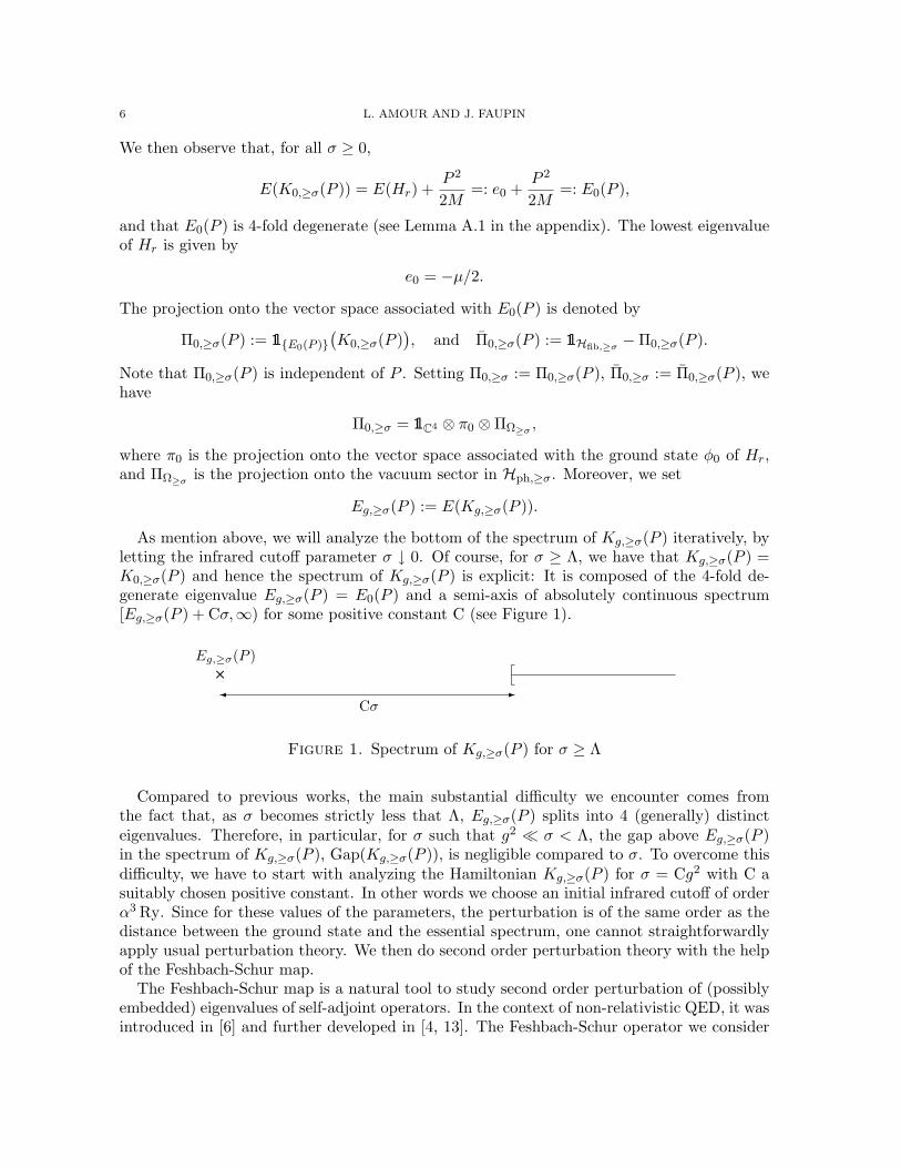
As mention above, we will analyze the bottom of the spectrum of Kg,≥σ(P ) iteratively, byletting the infrared cutoff parameter σ ↓ 0. Of course, for σ ≥ Λ, we have that Kg,≥σ(P ) =K0,≥σ(P ) and hence the spectrum of Kg,≥σ(P ) is explicit: It is composed of the 4-fold de-generate eigenvalue Eg,≥σ(P ) = E0(P ) and a semi-axis of absolutely continuous spectrum[Eg,≥σ(P ) + Cσ,∞) for some positive constant C (see Figure 1).

Cσ

..........................

-

Eg,≥σ(P ).................

.........

Figure 1. Spectrum of Kg,≥σ(P ) for σ ≥ Λ

Compared to previous works, the main substantial difficulty we encounter comes fromthe fact that, as σ becomes strictly less that Λ, Eg,≥σ(P ) splits into 4 (generally) distincteigenvalues. Therefore, in particular, for σ such that g2 σ < Λ, the gap above Eg,≥σ(P )in the spectrum of Kg,≥σ(P ), Gap(Kg,≥σ(P )), is negligible compared to σ. To overcome thisdifficulty, we have to start with analyzing the Hamiltonian Kg,≥σ(P ) for σ = Cg2 with C asuitably chosen positive constant. In other words we choose an initial infrared cutoff of orderα3 Ry. Since for these values of the parameters, the perturbation is of the same order as thedistance between the ground state and the essential spectrum, one cannot straightforwardlyapply usual perturbation theory. We then do second order perturbation theory with the helpof the Feshbach-Schur map.

The Feshbach-Schur map is a natural tool to study second order perturbation of (possiblyembedded) eigenvalues of self-adjoint operators. In the context of non-relativistic QED, it wasintroduced in [6] and further developed in [4, 13]. The Feshbach-Schur operator we consider


here is associated with Kg,≥σ(P )− Eg,≥σ(P ) and Π0,≥σ and is defined by

Fg,≥σ(P ) :=(E0(P )− Eg,≥σ(P ))Π0,≥σ −Π0,≥σWg,≥σ(P )[K0,≥σ(P )− Eg,≥σ(P ) + Π0,≥σWg,≥σ(P )Π0,≥σ

]−1Π0,≥σWg,≥σ(P )Π0,≥σ. (1.10)

We shall see in Section 2 that this operator is well-defined for suitable values of the parameters.The main property of Fg,≥σ(P ) that we shall use is that

Kg,≥σ(P )− Eg,≥σ(P ) ≥ Fg,≥σ(P ),

(see Lemma 2.2). Combined with the min-max principle, this operator inequality appears tobe very useful in the context of the present paper. In particular, it will allow us to prove thatthe spectrum of Kg,≥σ(P ) has the form pictured in Figure 2 (see Section 2): The bottom ofthe spectrum, Eg,≥σ(P ), is an isolated eigenvalue separated by a gap of size δg2 from threeother eigenvalues and a semi-axis of essential spectrum.

δg2

..........................

..........................

..........................

..........................

-

Eg,≥σ(P ).................

..........................

..........................

..........................

.........

Figure 2. Spectrum of Kg,≥σ(P ) for σ = Cg2, C 1

The key argument that allows the method to be applied is the decomposition of theFeshbach-Schur operator Fg,≥σ(P ), viewed as a 4× 4 matrix, into three parts,

Fg,≥σ(P ) = d(g) + g2Γ + Rem(g),

where d(g) is a scalar matrix and Γ is a matrix independent of g whose spectrum exhibits agap between its first and second eigenvalues. The remainder term, Rem(g), must be negligiblecompared to g2.

The rest of the proof borrows ideas from [22, 5, 2]. Namely, we shall prove (in Section 3)that if the ground state of Kg,≥σ(P ) is unique and if Gap(Kg,≥σ(P )) ≥ ησ, then the sameholds for Kg,≥τ (P ) with τ = κσ, 0 < κ < 1. This will show that for small σ’s, the spectrumof Kg,≥σ(P ) has the form pictured in Figure 3 (a non-degenerate eigenvalue separated from agap of size ησ from the rest of the spectrum). At the end, the parameters η and κ will haveto be carefully chosen, in relation with the initial analysis of Section 2.

ησ

..........................

-

Eg,≥σ(P ).................

.........

Figure 3. Spectrum of Kg,≥σ(P ) for σ ≤ C′g2, C′ 1

We conclude this section with introducing a few more notations related to the infrareddecomposition, which will be useful in Section 3. For 0 ≤ τ ≤ σ, let

H≤σph,≥τ := C⊕∞⊕n=1

Sn[L2((k, λ) ∈ R3 × 1, 2, τ ≤ |k| ≤ σ)⊗n

].


The vacuum in H≤σph,≥τ is denoted by Ω≤σ≥τ and the projection onto the vacuum sector isdenoted by Π

Ω≤σ≥τ. The Hilbert spaces Hfib,≥τ and Hfib,≥σ ⊗H≤σph,≥τ are isomorphic. We shall

sometimes not distinguish between the two of them. As an operator on Hfib,≥τ , we set

W≤σg,≥τ (P ) =− g

mel:((mel

M(P − Pph,≥τ ) + pr − gA≥σ(

mel

Mg

23 r))·A≤σ≥τ (

mel

Mg

23 r))

:

+g

mn:((mn

M(P − Pph,≥τ )− pr + gA≥σ(−mn

Mg

23 r))·A≤σ≥τ (−mn

Mg

23 r))

:

+g2

2mel:A≤σ≥τ (

mel

Mg

23 r)2: +

g2

2mn:A≤σ≥τ (−mn

Mg

23 r)2:

− g

2melσel ·B≤σ≥τ (

mel

Mg

23 r) +

g

2mnσn ·B≤σ≥τ (−mn

Mg

23 r), (1.11)

where A≤σ≥τ (·) and B≤σ≥τ (·) are given by the same expressions as A(·) and B(·) respectively,except that the integrals are taken over k ∈ R3, τ ≤ |k| ≤ σ. Note that

Hg,≥τ (P ) = Hg,≥σ(P ) +W≤σg,≥τ (P ).

Finally, in the case where τ = 0, the subindex ≥ 0 is removed from the notations above, thatis, for instance, H≤σph := H≤σph,≥0, W≤σg (P ) := W≤σg,≥0(P ) and so on.

Throughout the paper, the notation . · · · will stand for ≤ C · · · where C is a positiveconstant independent of the parameters. For any vector v, [v] and [v]⊥ will denote respectivelythe subspace spanned by v and its orthogonal complement.

2. Existence of a gap for large enough infrared cutoffs

In this section, we investigate the spectrum of the infrared cutoff Hamiltonian Kg,≥σ(P )for values of the coupling constant g and of the infrared cutoff parameter σ fixed such thatβ−1c2 g

2 ≤ σ ≤ β−1c1 g

2 (for some 0 < βc1 < βc2 to be determined later).For any small enough g and P , and for any σ, η > 0, let Gap(g, P, σ, η) denote the following

assertion:

Gap(g, P, σ, η)

(i) Eg,≥σ(P ) is a simple eigenvalue of Kg,≥σ(P ),(ii) Gap(Kg,≥σ(P )) ≥ ησ.

The main result of this section is the following.

Theorem 2.1. There exist pc > 0, βc2 > 0 and δ > 0 such that, for all 0 < βc1 < βc2, thereexists gc > 0 such that, for all 0 ≤ |P | ≤ pc, 0 < g ≤ gc and βc1 ≤ β ≤ βc2,

Gap(g, P, σ, δβ) holds,

where σ = g2β−1.

The statement of Theorem 2.1 expresses the fact that, for small enough values of thecoupling constant g and total momentum P , there is a gap at least of size δg2 in the spectrumof Kg,≥σ(P ) above the non-degenerate ground state eigenvalue Eg,≥σ(P ), provided that theinfrared cutoff parameter σ obeys β−1

c2 g2 ≤ σ ≤ β−1

c1 g2.


2.1. Preliminary lemmas. The proof of Theorem 2.1 relies on a few lemmas that we shallestablish in this preliminary subsection. For the convenience of the reader, some standardestimates used several times in the proofs below are recalled in Appendix A.

We begin with verifying that the Feshbach-Schur operator Fg,≥σ(P ) introduced in (1.10)is well-defined for suitable values of the parameters.

Lemma 2.2. There exist pc > 0 and βc2 > 0 such that, for all 0 < βc1 < βc2, there existsgc > 0 such that, for all 0 < g ≤ gc, 0 ≤ |P | ≤ pc and βc1 ≤ β ≤ βc2, the Feshbach-Schur operator defined in (1.10), Fg,≥σ(P ) (where σ = g2β−1), is a bounded operator onRan(Π0,≥σ) ⊂ Hfib given by

Fg,≥σ(P ) =(E0(P )− Eg,≥σ(P ))

)Π0,≥σ

−Π0,≥σWg,≥σ(P )[K0,≥σ(P )− Eg,≥σ(P )

]−1Π0,≥σWg,≥σ(P )Π0,≥σ

+ Rem1(g, P, β), (2.1)

where Rem1(g, P, β) is a bounded operator on Ran(Π0,≥σ) satisfying

‖Rem1(g, P, β)‖ . g2β12 . (2.2)

Moreover the following inequality holds in the sense of quadratic forms on D(Kg,≥σ(P )):

Kg,≥σ(P )− Eg,≥σ(P ) ≥ Fg,≥σ(P ). (2.3)

Proof. Let gc, pc, σc and CW be given by Lemma A.7. Let βc2 be such that β1/2c2 ≤ (6CW )−1,

and let 0 < βc1 < βc2. Possibly by considering a smaller gc, we can assume that g2c ≤ βc1σc

and hence, for all 0 < g ≤ gc and β ≥ βc1, we have that 0 < σ = g2β−1 ≤ σc. In addition weimpose that pc ≤M/2.

Fix g, P and β as in the statement of the lemma. By Lemmas A.1 and A.5, we have thatK0,≥σ(P )− Eg,≥σ(P ) is bounded invertible on Ran(Π0,≥σ) and satisfies(

K0,≥σ(P )− Eg,≥σ(P ))Π0,≥σ ≥

(E0(P )− Eg,≥σ(P ) + (1− |P |

M)σ)Π0,≥σ ≥

σ

2Π0,≥σ.

Using again that Eg,≥σ(P ) ≤ E0(P ) by Lemma A.5, it then follows from a straightforwardapplication of the Spectral Theorem that∥∥∥[K0,≥σ(P )− Eg,≥σ(P )

]−1Π0,≥σ(K0,≥σ(P )− E0(P ) + σ

)∥∥∥≤∥∥∥[K0,≥σ(P )− Eg,≥σ(P )

]−1Π0,≥σ(K0,≥σ(P )− Eg,≥σ(P ) + σ

)∥∥∥ ≤ 3. (2.4)

Moreover, by Lemma A.7, we have that∥∥∥[K0,≥σ(P )− E0(P ) + σ]− 1

2Wg,≥σ(P )[K0,≥σ(P )− E0(P ) + σ

]− 12

∥∥∥≤ CW gσ

− 12 = CWβ

12 , (2.5)

and hence∥∥∥[K0,≥σ(P )− Eg,≥σ(P )]− 1

2 Π0,≥σWg,≥σ(P )[K0,≥σ(P )− Eg,≥σ(P )

]− 12 Π0,≥σ

∥∥∥ ≤ 3CWβ12 .


Taking into account the choice of βc2, we have 3CWβ12 ≤ 1/2 so that in particular

(K0,≥σ(P )− Eg,≥σ(P )) Π0,≥σ + Π0,≥σWg,≥σ(P )Π0,≥σ

≥ 12

(K0,≥σ(P )− Eg,≥σ(P )) Π0,≥σ ≥σ

4Π0,≥σ. (2.6)

Therefore the operator (K0,≥σ(P )−Eg,≥σ(P ))Π0,≥σ+Π0,≥σWg,≥σ(P )Π0,≥σ is bounded invert-ible on Ran(Π0,≥σ). Using in addition that Wg,≥σ(P ) is relatively bounded with respect toK0,≥σ(P ), we obtain that Fg,≥σ(P ) is indeed a well-defined bounded operator on Ran(Π0,≥σ).

Next, using again (2.4) and (2.5), we obtain∥∥∥Π0,≥σWg,≥σ(P )[K0,≥σ(P )− Eg,≥σ(P )

]− 12 Π0,≥σ

∥∥∥ ≤ 2CWβ12σ

12 = 2CW g. (2.7)

A standard Neumann series decomposition together with the previous estimates then lead to

Π0,≥σWg,≥σ(P )[K0,≥σ(P )− Eg,≥σ(P ) + Π0,≥σWg,≥σ(P )Π0,≥σ

]−1Π0,≥σWg,≥σ(P )Π0,≥σ

= Π0,≥σWg,≥σ(P )[K0,≥σ(P )− Eg,≥σ(P )

]−1Π0,≥σWg,≥σ(P )Π0,≥σ + Rem1(g, P, β),

where Rem1(g, P, β) is a bounded operator on Ran(Π0,≥σ) satisfying (2.2).Finally, to prove (2.3), it suffices to use the following identity

Kg,≥σ(P )− Eg,≥σ(P ) = Fg,≥σ(P ) +R∗R, (2.8)

where

R :=[K0,≥σ(P )− Eg,≥σ(P ) + Π0,≥σWg,≥σ(P )Π0,≥σ

]− 12 Π0,≥σ(Kg,≥σ(P )− Eg,≥σ(P )).

We observe that the operator square root appearing in the expression of R is well-defined by(2.6). Equation (2.8) follows from straightforward algebraic computations (see e.g. [4, 13]).This concludes the proof of the lemma.

Our next task is to extract the second order term from (2.1). It is the purpose of thefollowing three lemmas.

Lemma 2.3. There exist gc > 0, pc > 0 and σc > 0 such that, for all 0 ≤ g ≤ gc, 0 ≤ |P | ≤ pcand 0 < σ ≤ σc,

Π0,≥σWg,≥σ(P )[K0,≥σ(P )− Eg,≥σ(P )

]−1Π0,≥σWg,≥σ(P )Π0,≥σ

=∑λ=1,2

∫R3

Π0,≥σw≥σ(r, k, λ)[Hr +

12M

(P − k)2 + |k| − Eg,≥σ(P )]−1

w≥σ(r, k, λ)Π0,≥σdk

+ Rem2(g, P, σ), (2.9)

where

w≥σ(r, k, λ) :=− g

mel

((mel


)· hA≥σ(

mel

Mg

23 r, k, λ)

)+

g

mn

((mn

M(P − Pph,≥σ)− pr

)· hA≥σ(−mn

Mg

23 r, k, λ)

)− g

2melσel · hB≥σ(

mel

Mg

23 r, k, λ) +

g

2mnσn · hB≥σ(−mn

Mg

23 r, k, λ), (2.10)

w≥σ(r, k, λ) is given by the same expression except that hA≥σ, hB≥σ are replaced by their conju-gate hA≥σ, hB≥σ, and Rem2(g, P, σ) is a bounded operator on Ran(Π0,≥σ) satisfying

‖Rem2(g, P, σ)‖ . g3.


Proof. It suffices to introduce the expression (1.9) of Wg,≥σ(P ) into the operator

Π0,≥σWg,≥σ(P )[K0,≥σ(P )− Eg,≥σ(P )

]−1Π0,≥σWg,≥σ(P )Π0,≥σ,

and next to estimate each term separately. An explicit computation then leads directly tothe statement of the lemma (see the proof of Lemma A.9 in [1] for more details).

Lemma 2.4. There exist gc > 0, pc > 0 and σc > 0 such that, for all 0 ≤ g ≤ gc, 0 ≤ |P | ≤ pc,0 < σ ≤ σc and λ ∈ 1, 2,∫

R3

Π0,≥σw≥σ(r, k, λ)[Hr +

12M

(P − k)2 + |k| − Eg,≥σ(P )]−1

w≥σ(r, k, λ)Π0,≥σdk

=∫

R3

Π0,≥σw≥σ(0, k, λ)[Hr +

12M

(P − k)2 + |k| − Eg,≥σ(P )]−1

w≥σ(0, k, λ)Π0,≥σdk

+ Rem3(g, P, σ, λ),

where w≥σ(0, k, λ) and w≥σ(0, k, λ) are defined by (2.10), and Rem3(g, P, σ, λ) is a boundedoperator on Ran(Π0,≥σ) satisfying

‖Rem3(g, P, σ, λ)‖ . g83 .

Proof. It follows from the definitions (1.4)–(1.5) of hAj and hBj that∣∣hAj,≥σ(r, k, λ)− hAj,≥σ(0, k, λ)∣∣ . 1|k|≥σ(k)|k|

12χΛ(k)|r|,∣∣hBj,≥σ(r, k, λ)− hBj,≥σ(0, k, λ)

∣∣ . 1|k|≥σ(k)|k|32χΛ(k)|r|,

for any j ∈ 1, 2, 3, λ ∈ 1, 2, r ∈ R3 and k ∈ R3. This implies that∥∥∥Π0,≥σ(mel


)·(hA≥σ(

mel

Mg

23 r, k, λ)− hA≥σ(0, k, λ)

)∥∥∥. g

231|k|≥σ(k)|k|

12χΛ(k)

∥∥∥Π0,≥σ(mel


)〈r〉∥∥∥

. g231|k|≥σ(k)|k|

12χΛ(k).

In the last inequality, we used in particular that ‖〈r〉prπ0‖ < ∞, where, recall, π0 is theprojection onto the ground state of the Schrodinger operator Hr. Similarly,∥∥∥Π0,≥σσ

el ·(hB≥σ(

mel

Mg

23 r, k, λ)− hB≥σ(0, k, λ)

)∥∥∥. g

231|k|≥σ(k)|k|

32χΛ(k)

∥∥∥Π0,≥σσel〈r〉

∥∥∥ . g 231|k|≥σ(k)|k|

32χΛ(k).

The same holds if mel is replaced by −mn and σel is replaced by σn. Besides, using thatHr + P 2/2M ≥ E0(P ) ≥ Eg,≥σ(P ) by Lemma A.5, we obtain that∥∥∥[Hr +

12M

(P − k)2 + |k| − Eg,≥σ(P )]−1

1|k|≥σ(k)∥∥∥

≤ 1−(k · P )/M + k2/2M + |k|

1|k|≥σ(k) ≤ 2|k|1|k|≥σ(k),

for |P | ≤M/2, and hence the statement of the lemma easily follows.


Lemma 2.5. There exist gc > 0, pc > 0 and σc > 0 such that, for all 0 ≤ g ≤ gc, 0 ≤ |P | ≤ pc,0 < σ ≤ σc, and λ ∈ 1, 2,∫

R3

Π0,≥σw≥σ(0, k, λ)[Hr +

12M

(P − k)2 + |k| − Eg,≥σ(P )]−1


= g2(ΓA,diag≥σ (P, λ) + ΓB≥σ(P, λ)

)+ Rem4(g, P, σ, λ),

where

ΓA,diag≥σ (P, λ) :=

1µ2

∫R3

Π0,≥σpr · hA≥σ(0, k, λ)[Hr +

12M

(P − k)2 + |k| − E0(P )]−1

(1C4 ⊗ π0 ⊗ 1Hph)pr · hA≥σ(0, k, λ)Π0,≥σdk,

and

ΓB≥σ(P, λ) :=∫

R3

Π0,≥σ

(− 1

2melσel · hB≥σ(0, k, λ) +

12mn

σn · hB≥σ(0, k, λ))

[e0 +

12M

(P − k)2 + |k| − E0(P )]−1

(− 1


12mn

σn · hB≥σ(0, k, λ))

Π0,≥σdk.

Moreover Rem4(g, P, σ, λ) is a bounded operator on Ran(Π0,≥σ) satisfying

‖Rem4(g, P, σ, λ)‖ . g4.

Proof. It follows from (2.10) that

w≥σ(0, k, λ) =− g

µpr · hA≥σ(0, k, λ)− g


g

2mnσn · hB≥σ(0, k, λ),

and likewise for w≥σ(0, k, λ) except that hA≥σ, hB≥σ are replaced by hA≥σ, hB≥σ. (Observe inparticular that the terms proportional to (P − Pph) vanish. This is due to the fact that thecharge of the total system we consider vanishes).

Moreover, we have that hA≥σ(0, k, λ) = hA≥σ(0, k, λ) and

Π0,≥σpr · hA≥σ(0, k, λ)(1C4 ⊗ π0 ⊗ 1Hph) = 0.

This yields∫R3

Π0,≥σw≥σ(0, k, λ)[Hr +

12M

(P − k)2 + |k| − Eg,≥σ(P )]−1


= g2(ΓA,diag≥σ (g, P, λ) + ΓB≥σ(g, P, λ)

),

where

ΓA,diag≥σ (g, P, λ) :=

1µ2

∫R3

Π0,≥σpr · hA≥σ(0, k, λ)[Hr +

12M

(P − k)2 + |k| − Eg,≥σ(P )]−1

(1C4 ⊗ π0 ⊗ 1Hph)pr · hA≥σ(0, k, λ)Π0,≥σdk,


and

ΓB≥σ(g, P, λ) :=∫

R3

Π0,≥σ

(− 1


12mn

σn · hB≥σ(0, k, λ))

[e0 +

12M

(P − k)2 + |k| − Eg,≥σ(P )]−1

(− 1


12mn

σn · hB≥σ(0, k, λ))

Π0,≥σdk.

For any |P | ≤M/2 and |k| ≥ σ, we have that∥∥∥[Hr +1

2M(P − k)2 + |k| − E0(P )

]−1(1C4 ⊗ π0 ⊗ 1 Hph)∥∥∥ ≤ 1

e1 − e0,

and hence also that∥∥∥[Hr +1

2M(P − k)2 + |k| − Eg,≥σ(P )

]−1(1C4 ⊗ π0 ⊗ 1Hph)∥∥∥ ≤ 1

e1 − e0,

by Lemma A.5. Therefore, using the first resolvent equation together with the facts that|E0(P )−Eg,≥σ(P )| . g2 (see Lemma A.5) and |hA≥σ(0, k, λ)| . 1|k|≥σ(k)|k|−1/2χΛ(k), we get

ΓA,diag≥σ (g, P, λ) = ΓA,diag

≥σ (P, λ) + RemA(g, P, σ),

where

‖RemA(g, P, σ)‖ . g2

∫R3

1σ≤|k|≤Λdk|k|. g2.

Likewise, for any |P | ≤M/2 and |k| ≥ σ, we have that∣∣[e0 +1

2M(P − k)2 + |k| − Eg,≥σ(P )

]−1∣∣ ≤ 2|k|,

and since |hB≥σ(0, k, λ)| . 1|k|≥σ(k)|k|1/2χΛ(k), we thus obtain that

ΓB≥σ(g, P, λ) = ΓB≥σ(P, λ) + RemB(g, P, σ),

where

‖RemB(g, P, σ)‖ . g2

∫R3

1σ≤|k|≤Λdk|k|. g2.

Hence the lemma is proven.

To conclude this subsection, we estimate the size of the splitting induced by the secondorder term in (2.2). Since the matrix ΓA,diag

≥σ (P, λ) of Lemma 2.5 is scalar, only ΓB≥σ(P, λ) isresponsible for this splitting.

From now on, to simplify a few computations and since the system is rotation invariant,we choose the total momentum P to be directed along −→ε3 .

Lemma 2.6. There exist pc > 0 and σc > 0 such that, for all P = P3−→ε3 satisfying 0 ≤ |P | ≤

pc, for all 0 < σ ≤ σc, and λ ∈ 1, 2,

ΓB≥σ(P, λ) = ΓB,diag≥σ (P, λ) + ΓB,#≥σ (P, λ),


where ΓB,diag≥σ (P, λ) is the scalar operator on Ran Π0,≥σ given by

ΓB,diag≥σ (P, λ) :=

( 14m2

el

+1

4m2n

)∫R3

∣∣hB≥σ(0, k, λ)∣∣2dk

|k| − (k · P )/M + k2/2MΠ0,≥σ,

and

ΓB,#≥σ (P, λ) := − 12melmn

∑j=1,2,3

∫R3

∣∣hBj,≥σ(0, k, λ)∣∣2dk

|k| − (k · P )/M + k2/2MΠ0,≥σσ

elj σ

nj Π0,≥σ.

Proof. Using standard properties of the Pauli matrices (see Lemma A.10), since for any k ∈ R3

and λ ∈ 1, 2, hB≥σ(0, k, λ) = −hB≥σ(0, k, λ), we have that(σel · hB≥σ(0, k, λ)

)(σel · hB≥σ(0, k, λ)

)= −(hB≥σ(0, k, λ))2 =

∣∣hB≥σ(0, k, λ)∣∣2,

and likewise with σn replacing σel. Next, we observe that for P = P3−→ε3 , λ ∈ 1, 2 and

j, j′ ∈ 1, 2, 3, j 6= j′, ∫R3

hBj,≥σ(0, k, λ)hBj′,≥σ(0, k, λ)

|k| − (k · P )/M + k2/2Mdk = 0.

The lemma then follows straightforwardly from the expression of ΓB≥σ(P, λ) given in thestatement of Lemma 2.5.

Lemma 2.7. There exist pc > 0 and σc > 0 such that, for all P = P3−→ε3 satisfying 0 ≤ |P | ≤ pc

and for all 0 < σ ≤ σc, the eigenvalues of the operator

ΓB,#≥σ (P ) := −∑λ=1,2

ΓB,#≥σ (P, λ)

are given by

γ(0)≥σ(P ) := − 1

8melmnπ2

∫R3

|k|1σ≤|k|≤Λ(k)|k| − (k · P )/M + k2/2M

dk,

γ(j)≥σ(P ) :=

18melmnπ2

∫R3

|k|1σ≤|k|≤Λ(k)|k| − (k · P )/M + k2/2M

k2j

|k|2dk, j = 1, 2, 3.

Proof. It directly follows from the properties of the Pauli matrices (see Lemma A.11).

Remarks 2.8.(1) For P = 0, we observe that γ(1)

≥σ(0) = γ(2)≥σ(0) = γ

(3)≥σ(0). It may however not be the

case for P 6= 0.(2) The gap above the lowest eigenvalue γ(0)

≥σ(P ) is non-vanishing. More precisely, letting

δ≥σ(P ) := min(γ

(1)≥σ(P ), γ(2)

≥σ(P ), γ(3)≥σ(P )

)− γ(0)≥σ(P ),

and

δ := inf0≤|P |≤pc,0≤σ≤Λ/2

δ≥σ(P ),

we have

δ ≥ 18melmnπ2

∫R3

|k|1Λ/2≤|k|≤Λ(k)(1 + pc/M)|k|+ k2/2M

dk > 0.


2.2. Proof of Theorem 2.1.Proof of Theorem 2.1. Let pc be fixed as the minimum of the pc’s given by Lemmas 2.2–2.7and A.5, and let CW be given by Lemma A.7. Let σc = βc2 = ε where ε > 0 is a small, fixedparameter (smaller, in particular, than the minimum of the σc’s given by Lemmas 2.3–2.7 andthan the βc2’s given by Lemma 2.2). Let now 0 < βc1 < βc2 and let gc be fixed smaller thanthe minimum of the gc’s given by Lemmas 2.2–2.7. We recall in particular from the proofs ofLemma 2.2 that g2

c ≤ βc1σc, which implies that for all 0 < g ≤ gc and β ≥ βc1, we have that0 < σg,β ≤ σc, with σg,β = g2β−1.

Let 0 ≤ |P | ≤ pc, 0 < g ≤ gc, βc1 ≤ β ≤ βc2. By rotation invariance, we can assumethat P = P3

−→ε3 . Before starting the proof we introduce a few more notations to simplifyexpressions. Combining Lemmas 2.2–2.6, we can write

Fg,≥σ(P ) =(E0(P )− Eg,≥σ(P ))Π0,≥σ + g2d≥σ(P )Π0,≥σ + g2ΓB,#≥σ (P ) + Rem(g, P, β),

where d≥σ(P ) is the (scalar) bounded operator on Ran(Π0,≥σ) defined by

d≥σ(P ) :=−∑λ=1,2

(ΓA,diag≥σ (P, λ) + ΓB,diag

≥σ (P, λ)),

and Rem(g, P, β) is a bounded operator on Ran(Π0,≥σ) satisfying

‖Rem(g, P, β)‖ . g2(β12 + g + 2g

23 + 2g2) . g2ε

12 . (2.11)

Here we used that, by assumption, β and g are smaller than ε. We also introduce the operator

F (2) :=Fg,≥σ(P ) + Eg,≥σ(P )Π0,≥σ − Rem(g, P, β)

=(E0(P ) + g2d≥σ(P )

)Π0,≥σ + g2ΓB,#≥σ (P ).

Identifying d≥σ(P ) with a scalar quantity, the lowest eigenvalue of F (2) is, according to Lemma2.7, given by

e(0)≥σ(P ) := E0(P ) + g2(d≥σ(P ) + γ

(0)≥σ(P )).

Moreover, it follows again from Lemma 2.7 that e(0)≥σ(P ) is simple and that

Gap(F (2)) ≥ g2δ≥σ(P ) ≥ g2δ, (2.12)

on Ran(Π0,≥σ), where δ≥σ(P ) and δ > 0 are given by Remark 2.8 (2).Let φ(0)

≥σ(P ) ∈ Ran(Π0,≥σ) denote a normalized eigenstate associated with the eigenvalue

e(0)≥σ(P ) of F (2).

Step 1 Let us prove that

e(0)≥σ(P ) ≥ Eg,≥σ(P )− g2δ

4. (2.13)

Let ψ(0)≥σ(P ) be the following trial state:

ψ(0)≥σ(P ) := φ

(0)≥σ(P )−

[K0,≥σ(P )− Eg,≥σ(P ) + Π0,≥σWg,≥σ(P )Π0,≥σ

]−1

Π0,≥σWg,≥σ(P )φ(0)≥σ(P ).


We observe that 〈ψ(0)≥σ(P ), φ(0)

≥σ(P )〉 = 〈φ(0)≥σ(P ), φ(0)

≥σ(P )〉 = 1. Proceeding as in the proof ofLemma 2.2, using (2.6) and (2.7), we find that

‖ψ(0)≥σ(P )− φ(0)

≥σ(P )‖ ≤ 4√

2CWβ12 . ε

12 , (2.14)

where we used that β1/2 ≤ ε1/2. Moreover, using the properties of the Feshbach operator, weobtain that

Π0,≥σ(Kg,≥σ(P )− Eg,≥σ(P )

)ψ

(0)≥σ(P )

= Fg,≥σ(P )φ(0)≥σ(P )

=(e

(0)≥σ(P )− Eg,≥σ(P )

)φ

(0)≥σ(P ) + Rem(g, P, β)φ(0)

≥σ(P ),

and

Π0,≥σ(Kg,≥σ(P )− Eg,≥σ(P )

)ψ

(0)≥σ(P )

= Π0,≥σWg,≥σ(P )φ(0)≥σ(P )− Π0,≥σWg,≥σ(P )φ(0)

≥σ(P ) = 0.

Therefore we deduce that

0 ≤⟨ψ

(0)≥σ(P ),

(Kg,≥σ(P )− Eg,≥σ(P )

)ψ

(0)≥σ(P )

⟩= e

(0)≥σ(P )− Eg,≥σ(P ) + 〈ψ(0)

≥σ(P ),Rem(g, P, β)φ(0)≥σ(P )〉

≤ e(0)≥σ(P )− Eg,≥σ(P ) + ‖ψ(0)

≥σ(P )‖‖Rem(g, P, β)‖

≤ e(0)≥σ(P )− Eg,≥σ(P ) + Cg2ε

12 ,

where in the last inequality we used (2.14) and (2.11). Hence, choosing ε1/2 δ, (2.13) isproven.

Step 2 Let µ2 denote the second point above Eg,≥σ(P ) in the spectrum of Kg,≥σ(P ). Themin-max principle implies that

µ2 ≥ infψ ∈ D(Kg,≥σ(P )), ‖ψ‖ = 1,

ψ ∈ [φ(0)≥σ(P )]⊥

〈ψ,Kg,≥σ(P )ψ〉.

Now, for ψ as above, using inequality (2.3) of Lemma 2.2, we can write

〈ψ,Kg,≥σ(P )ψ〉 ≥ 〈ψ,Fg,≥σ(P )ψ〉+ Eg,≥σ(P )

≥ 〈ψ,F (2)ψ〉+ 〈ψ,Rem(g, P, β)ψ〉.

Since F (2)Π0,≥σ = 0 and since ψ ∈ [φ(0)≥σ(P )]⊥, it follows from (2.12) that

〈ψ, F (2)ψ〉 ≥ (e(0)≥σ(P ) + g2δ)‖Π0,≥σψ‖2 ≥ e(0)

≥σ(P ) + g2δ.

In the last inequality, we used that E0(P ) = P 2/2M + e0 = P 2/2M − µ/2 is negative for|P | ≤ pc small enough, and hence that e(0)

≥σ(P ) + g2δ is also negative for g and |P | smallenough. Moreover, (2.11) yields

〈ψ,Rem(g, P, β)ψ〉 ≥ −Cg2ε12 .


Thus, applying Step 1, we obtain that

µ2 ≥ Eg,≥σ(P ) +34g2δ − Cg2ε

12 ≥ Eg,≥σ(P ) +

12g2δ,

provided ε is small enough. Changing notations (δ/2→ δ), this implies the statement of thetheorem.

3. Proof of Theorem 1.1

The main theorem of this section, which will allow us to prove Theorem 1.1, is the following.

Theorem 3.1. There exist gc > 0, pc > 0 and 0 < η ≤ 1/4 such that, for all 0 < g ≤ gc and0 ≤ |P | ≤ pc, there exist σc > 0 such that for all 0 < σ ≤ σc,

Gap(g, P, σ, η) holds.

We need the following two lemmas before starting the proof of Theorem 3.1.

Lemma 3.2. Let gc > 0, σc > 0 and pc > 0 be fixed small enough and let 0 ≤ g ≤ gc, 0 ≤ σ ≤σc and 0 ≤ |P | ≤ pc be such that Gap(g, P, σ, η) holds. Let Φg,≥σ(P ) be a normalized groundstate of Kg,≥σ(P ). For all 0 ≤ τ ≤ σ, Eg,≥σ(P ) is a simple eigenvalue of Hg,≥σ(P )|Hfib,≥τ

associated with the normalized ground state Φg,≥σ(P )⊗ Ω≤σ≥τ , and

Gap(Hg,≥σ(P )|Hfib,≥τ ) ≥ min(ησ,τ

4).

Proof. First, one can readily verifies that Φg,≥σ(P )⊗Ω≤σ≥τ is an eigenstate of Hg,≥σ(P )|Hfib,≥τ

associated with the eigenvalue Eg,≥σ(P ). Since

1Hfib,≥τ −(Πg,≥σ(P )⊗Π

Ω≤σ≥τ

)=(1Hfib,≥σ −Πg,≥σ(P )

)⊗Π

Ω≤σ≥τ

+ 1Hfib,≥σ ⊗(1H≤σph,≥τ

−ΠΩ≤σ≥τ

), (3.1)

and since 1H≤σph,≥τ⊗Π

Ω≤σ≥τcommutes with Hg,≥σ(P )|Hfib,≥τ , we have that

infψ ∈ D(Hg,≥σ(P )|Hfib,≥τ ), ‖ψ‖ = 1,

ψ ∈ [Φg,≥σ(P )⊗ Ω≤σ≥τ ]⊥

〈ψ,Hg,≥σ(P )|Hfib,≥τψ〉

≥ min(


ψ ∈ [Φg,≥σ(P )]⊥ ⊗ [Ω≤σ≥τ ]

〈ψ,Hg,≥σ(P )|Hfib,≥τψ〉,


ψ ∈ Hfib,≥σ ⊗ [Ω≤σ≥τ ]⊥

〈ψ,Hg,≥σ(P )|Hfib,≥τψ〉). (3.2)

The assumption that Gap(Kg,≥σ(P )) ≥ ησ yields that


ψ ∈ [Φg,≥σ(P )]⊥ ⊗ [Ω≤σ≥τ ]

〈ψ,Hg,≥σ(P )|Hfib,≥τψ〉 ≥ Eg,≥σ(P ) + ησ.

To estimate from below the second term in the right-hand-side of (3.2), we use the fact thatHg,≥σ(P )|Hfib,≥τ commutes with the number operator 1Hfib,≥σ ⊗ N

≤σph,≥τ (defined in (A.4)).


We then consider ψ ∈ D(Hg,≥σ(P )|Hfib,≥τ ) such that ‖ψ‖ = 1 and 1Hfib,≥σ ⊗ N≤σph,≥τψ = nψ

with n ≥ 1. This state ψ may be seen as an element of L2((k, λ), τ ≤ |k| ≤ σ;Hfib,≥σ ⊗L2((k, λ), τ ≤ |k| ≤ σn−1)), and we have that

〈ψ,Hg,≥σ(P )|Hfib,≥τψ〉

=∑λ=1,2

∫τ≤|k|≤σ

⟨(ψ(k, λ), Hg,≥σ(P − k)|Hfib,≥σ⊗L2((k,λ),τ≤|k|≤σn−1) + |k|

)ψ(k, λ)

⟩dk

≥ infτ≤|k|≤σ

(Eg,≥σ(P − k) + |k|

)≥ Eg,≥σ(P ) +

τ

4,

where the last inequality is a consequence of Lemma A.2. Therefore we obtain that


ψ ∈ Hfib,≥σ ⊗ [Ω≤σ≥τ ]⊥

〈ψ,Hg,≥σ(P )|Hfib,≥τψ〉 ≥ Eg,≥σ(P ) +τ

4,

which concludes the proof of the lemma.

Lemma 3.3. There exists pc > 0 such that, for all η and κ such that 0 < 4η ≤ κ < 1, thereexists gc > 0 such that, for all 0 ≤ g ≤ gc, 0 ≤ |P | ≤ pc and σ > 0

Gap(g, P, σ, η)⇒ Gap(g, P, κσ, η).

Proof. Assume that Gap(g, P, σ, η) is satisfied for some σ > 0. Let Φg,≥σ(P ) be a groundstate of Kg,≥σ(P ). Let τ = κσ and let µ2 denote the first point above Eg,≥τ (P ) in thespectrum of Kg,≥τ (P ). By the min-max principle,

µ2 ≥ infψ ∈ D(Kg,≥τ (P )), ‖ψ‖ = 1ψ ∈ [Φg,≥σ(P )⊗ Ω≤σ≥τ ]⊥

〈ψ,Kg,≥τ (P )ψ〉,

where [Φg,≥σ(P )⊗Ω≤σ≥τ ]⊥ denotes the orthogonal complement of the vector space spanned byΦg,≥σ(P )⊗Ω≤σ≥τ in Hfib,≥σ⊗H≤σph,≥τ ' Hfib,≥τ . It follows from Lemma A.8 that for any ρ > 0,

〈ψ,Kg,≥τ (P )ψ〉 = 〈ψ,Hg,≥σ(P )|Hfib,≥τψ〉+ 〈ψ,W≤σg,≥τ (P )ψ〉

≥[1− CW gσ

1/2ρ−1/2]〈ψ,Hg,≥σ(P )|Hfib,≥τψ〉

+ CW gσ1/2ρ−1/2Eg,≥σ(P )− CW gσ

1/2ρ1/2.

Next, by Gap(g, P, σ, η), Lemma 3.2 and the fact that τ = κσ ≥ 4ησ, we obtain that for anyψ in [Φg,≥σ(P )⊗ Ω≤σ≥τ ]⊥, ‖ψ‖ = 1,

〈ψ,Hg,≥σ(P )|Hfib,≥τψ〉 ≥ Eg,≥σ(P ) + ησ,

provided that g is sufficiently small. Hence for any ρ > 0 such that ρ1/2 > CW gσ1/2,

〈ψ,Kg,≥τ (P )ψ〉 ≥ Eg,≥σ(P ) +[1− CW gσ

1/2ρ−1/2]ησ − CW gσ

1/2ρ1/2.

Choosing ρ1/2 = 2(1− κ)−1CW gσ1/2 and using Lemma A.6, we get

〈ψ,Kg,≥τ (P )ψ〉 ≥ Eg,≥σ(P ) +1 + κ

2ησ − 2(1− κ)−1C2

W g2σ

≥ Eg,≥τ (P ) + ητ +1− κ

2ησ − 2(1− κ)−1C2

W g2σ.


Hence µ2 ≥ Eg,≥τ (P )+ητ provided that g2 ≤ (4C2W )−1(1−κ)2η, which proves the lemma.

Let us now prove Theorem 3.1.

Proof of Theorem 3.1. Let pc be the minimum of the pc’s given by Theorem 2.1 and Lemma3.3. Let βc2 and δ be given by Theorem 2.1. Note that, possibly by considering a smallerβc2, we can assume that 4δ < β−1

c2 . Fix βc1 such that 0 < βc1 < βc2. Let η := δβc1 andκ := βc1β

−1c2 . In particular we have that 0 < 4η ≤ κ < 1. Let gc be the minimum of the gc’s

given by Theorem 2.1 and Lemma 3.3.Let 0 < g ≤ gc and 0 ≤ |P | ≤ pc. By rotation invariance, we can assume that P = P3

−→ε3 .Let σc := g2β−1

c1 . By Theorem 2.1, we know that, for all σ such that g2β−1c2 ≤ σ ≤ g2β−1

c1 ,Gap(g, P, σ, η) holds. Using Lemma 3.3, this implies that, for all σ such that g2β−1

c2 ≤σ ≤ g2β−1

c1 and for all n ∈ N0, Gap(g, P, κnσ, η) holds. Since κ = βc1β−1c2 , we deduce that

Gap(g, P, σ, η) is satisfied for all 0 < σ ≤ g2β−1c1 , which concludes the proof of the theorem.

We are now able to prove the main theorem of this paper.

Proof of Theorem 1.1. Let gc > 0, pc > 0 and 0 < η ≤ 1/4 be given by Theorem 3.1 and letCW be given by Lemma A.8. Let 0 < g ≤ gc and 0 ≤ |P | ≤ pc. By rotation invariance, wecan assume without loss of generality that P = P3

−→ε3 . Let σc > 0 be given by Theorem 3.1.For 0 < σ ≤ σc, let Φg,≥σ(P ) denote a normalized ground state of Kg,≥σ(P ). Recall

from Lemma 3.2 that Φg,≥σ(P ) ⊗ Ω≤σ is then a normalized ground state of Hg,≥σ(P ). Bythe Banach-Alaoglu theorem, there exists a sequence (Φg,≥σn(P )⊗Ω≤σn)n∈N which convergesweakly as n→∞, with 0 < σn ≤ min(σc, 1) and σn → 0. Let Φg(P ) denote the correspondinglimit. One easily verifies that Hg(P )Φg(P ) = Eg(P )Φg(P ). To prove that Φg(P ) 6= 0, wedecompose

1 = 〈Φg,≥σn(P )⊗ Ω≤σn ,Φg,≥σn(P )⊗ Ω≤σn〉= 〈Φg,≥σn(P )⊗ Ω≤σn ,

((1C4 ⊗ π0 ⊗ΠΩ≥σn

)Φg,≥σn(P ))⊗ Ω≤σn〉

+ 〈Φg,≥σn(P )⊗ Ω≤σn ,((1C4 ⊗ π0 ⊗ΠΩ≥σn

)Φg,≥σn(P ))⊗ Ω≤σn〉

+ 〈Φg,≥σn(P )⊗ Ω≤σn ,((1C4 ⊗ 1L2(R3) ⊗ ΠΩ≥σn

)Φg,≥σn(P ))⊗ Ω≤σn〉.

By Lemma A.9, the second term in the r.h.s. is bounded by O(g2). Likewise, since ΠΩ≥σn≤

Nph,≥σnΠΩ≥σn, Lemma A.3 implies that the last term in the r.h.s. is also bounded by O(g2).

Letting αj , j = 1, . . . , 4, denote an orthonormal basis of C4, and taking the limit n→∞, wededuce that ∑

j=1,...,4

∣∣〈Φg(P ), αj ⊗ φ0 ⊗ Ω〉|2 ≥ 1−O(g2).

Hence Φg(P ) 6= 0, and it follows that Φg(P ) is a normalized ground state of Hg(P ).In order to prove Theorem 1.1, it now suffices to follow [5]. Assume by contradiction that

there exists another normalized ground state, say Φ′g(P ), such that 〈Φg(P ),Φ′g(P )〉 = 0. We


write∣∣〈Φg(P ),Φ′g(P )〉∣∣2 = lim

n→∞

∣∣〈Φg,≥σn(P )⊗ Ω≤σn ,Φ′g(P )〉∣∣2

= limn→∞

⟨Φ′g(P ),1Eg,≥σn (P )(Hg,≥σn(P ))Φ′g(P )

⟩= 1− lim

n→∞

⟨Φ′g(P ), (1Hfib

− 1Eg,≥σn (P )(Hg,≥σn(P )))Φ′g(P )⟩. (3.3)

Notice that, in the second equality, we used the fact that, by Theorem 3.1 and Lemma 3.2,Eg,≥σn(P ) is a simple eigenvalue of Hg,≥σn(P ). We decompose

1Hfib− 1Eg,≥σn (P )(Hg,≥σn(P )) =(1Hfib,≥σn

− 1Eg,≥σn (P )(Kg,≥σn(P )))⊗ΠΩ≤σn

+ 1Hfib,≥σn⊗ (1H≤σnph

−ΠΩ≤σn ), (3.4)

and use that, by Lemma A.4,⟨Φ′g(P ),1Hfib,≥σn

⊗ (1H≤σnph−ΠΩ≤σn )Φ′g(P )

⟩≤⟨Φ′g(P ),N≤σnph Φ′g(P )

⟩. g2σ2

n . g2. (3.5)

On the other hand, by Theorem 3.1, we can write⟨Φ′g(P ), (1Hfib,≥σn

− 1Eg,≥σn (P )(Kg,≥σn(P )))⊗ΠΩ≤σnΦ′g(P )⟩

≤ 1ησn

⟨Φ′g(P ), (Kg,≥σn(P )− Eg,≥σn(P ))⊗ΠΩ≤σnΦ′g(P )

⟩=

1ησn

⟨Φ′g(P ), (Hg,≥σn(P )− Eg,≥σn(P ))(1⊗ΠΩ≤σn )Φ′g(P )

⟩≤ 1ησn

⟨Φ′g(P ), (Hg,≥σn(P )− Eg,≥σn(P ))Φ′g(P )

⟩=

1ησn

⟨Φ′g(P ), (Eg(P )− Eg,≥σn(P )−W≤σng (P ))Φ′g(P )

⟩,

where in the last equality we used that (Hg(P ) − Eg(P ))Φ′g(P ) = 0 and that Hg(P ) =Hg,≥σn(P ) +W≤σng (P ). By Lemmas A.6 and A.8, this implies that⟨

Φ′g(P ), (1Hfib,≥σn − 1Eg,≥σn (P )(Kg,≥σn(P )))⊗ΠΩ≤σnΦ′g(P )⟩≤ Cg2σn

η+

CW g

η. g, (3.6)

since σn ≤ 1. Combining (3.4), (3.5) and (3.6), we obtain that, for g small enough, (3.3) > 0,which is a contradiction. Hence the theorem is proven.

Appendix A. Known results and standard estimates

This appendix contains several already known results and fairly standard estimates whichwere used above.

Lemma A.1. For all 0 ≤ |P | < M , and σ ≥ 0, we have that

K0,≥σ(P )− E0(P ) ≥(1− |P |

M

)Hph,≥σ. (A.1)

Moreover, the spectrum of K0,≥σ(P ) satisfies

spec(K0,≥σ(P )) ⊆E0(P )

∪[E0(P ) +

(1− |P |

M

)σ,+∞), (A.2)


and

dim Ker(K0,≥σ(P )− E0(P )

)= 4. (A.3)

Proof. Recall that

K0,≥σ(P ) = Hr +P 2

2M− 1MP · Pph,≥σ +

12M

P 2ph,≥σ +Hph,≥σ,

on the Hilbert space Hfib,≥σ. For Φ ∈ D(K0,≥σ(P )), we have that

|〈Φ, P · Pph,≥σΦ〉| ≤ |P |〈Φ, Hph,≥σΦ〉.Therefore,

K0,≥σ(P ) ≥ e0 +P 2

2M+(1− |P |

M

)Hph,≥σ,

which proves (A.1).In order to prove (A.2) and (A.3), it suffices to observe that

K0,≥σ(P )(y ⊗ φ0 ⊗ Ω≥σ) = E0(P )(y ⊗ φ0 ⊗ Ω≥σ),

for any y ∈ C4, and that, by (A.1), if ψ ∈ D(K0,≥σ(P )) satisfies ‖ψ‖ = 1 and 〈ψ, (y ⊗ φ0 ⊗Ω≥σ)〉 = 0 for all y ∈ C4, then

〈ψ, (K0,≥σ(P )− E0(P ))ψ〉 ≥(1− |P |

M

)σ.

Hence the lemma follows.

The next result is proven in [3, Lemma 4.3]. This type of inequality is an importantingredient in the proof of the existence of a ground state for translation invariant models innon-relativistic QED (see e.g. [11, 22, 3, 20]).

Lemma A.2. There exist gc > 0, pc > 0 and σc > 0 such that, for all 0 ≤ g ≤ gc,0 ≤ |P | ≤ pc, 0 ≤ σ ≤ σc and k ∈ R3,

Eg,≥σ(P − k)− Eg,≥σ(P ) ≥ −34|k|.

The number operator of particles of energies ≥ σ is defined by

Nph,≥σ :=∑λ=1,2

∫|k|≥σ

a∗λ(k)aλ(k)dk.

The following two lemmas are easy generalizations of [3, Lemma 4.5] based on the combinationof a pull-through formula together with a Pauli-Fierz transformation (see also [6, 14]). Wedo not recall the proofs.

Lemma A.3. There exist gc > 0, pc > 0 and σc > 0 such that, for all 0 ≤ g ≤ gc, 0 ≤ |P | ≤ pcand 0 ≤ σ ≤ σc, Ker(Kg,≥σ(P ) − Eg,≥σ(P )) ⊂ D(N 1/2

ph,≥σ), and the following holds: For allΦg,≥σ(P ) ∈ Ker(Kg,≥σ(P )− Eg,≥σ(P )), ‖Φg,≥σ(P )‖ = 1, we have that

〈Φg,≥σ(P ),Nph,≥σΦg,≥σ(P )〉 . g2.

In the next lemma, we use the notation

N≤σph,≥τ :=∑λ=1,2

∫τ≤|k|≤σ

a∗λ(k)aλ(k)dk. (A.4)


Lemma A.4. There exist gc > 0, pc > 0 and σc > 0 such that, for all 0 ≤ g ≤ gc, 0 ≤ |P | ≤ pcand 0 ≤ τ ≤ σ ≤ σc, Ker(Kg,≥τ (P ) − Eg,≥τ (P )) ⊂ D((N≤σph,≥τ )1/2), and the following holds:For all Φg,≥τ (P ) ∈ Ker(Kg,≥τ (P )− Eg,≥τ (P )), ‖Φg,≥τ (P )‖ = 1, we have that

〈Φg,≥τ (P ),N≤σph,≥τΦg,≥τ (P )〉 . g2σ2.

The next lemma is proven in the same way as Lemma A.6 in [1]. We do not reproduce theproof here.

Lemma A.5. There exist gc > 0, pc > 0, σc > 0 and C0 > 0 such that, for all 0 ≤ g ≤ gc,0 ≤ |P | ≤ pc, and 0 ≤ σ ≤ σc,

Eg,≥σ(P ) ≤ E0(P ) ≤ Eg,≥σ(P ) + C0g2.

Similarly we have the following:

Lemma A.6. There exist gc > 0, pc > 0, σc > 0 and C0 > 0 such that, for all 0 ≤ g ≤ gc,0 ≤ |P | ≤ pc, and 0 ≤ τ ≤ σ ≤ σc,

Eg,≥τ (P ) ≤ Eg,≥σ(P ) ≤ Eg,≥τ (P ) + C0g2σ2. (A.5)

Proof. Again, the proof is similar to the one of Lemma A.6 in [1]. We only sketch the maindifferences here. Recall that

Kg,≥τ (P ) = Hg,≥σ(P )|Hfib,≥τ +W≤σg,≥τ (P ), (A.6)

in Hfib,≥τ , where W≤σg,≥τ (P ) is given in (1.11). By Lemma 3.2,

Hg,≥σ(P )|Hfib,≥τ

(Φg,≥σ(P )⊗ Ω≤σ≥τ

)= Eg,≥σ(P )Φg,≥σ(P )⊗ Ω≤σ≥τ .

Thus, the first inequality in (A.5) follows from

Eg,≥τ (P ) ≤⟨Φg,≥σ(P )⊗ Ω≤σ≥τ ,Kg,≥τ (P )Φg,≥σ(P )⊗ Ω≤σ≥τ

⟩= Eg,≥σ(P ),

since W≤σg,≥τ (P ) is Wick ordered.In order to prove the second inequality in (A.5), we use that, by (A.6),

Eg,≥σ(P ) ≤⟨Φg,≥τ (P ), Hg,≥σ(P )|Hfib,≥τΦg,≥τ (P )

⟩≤ Eg,≥τ (P )−

⟨Φg,≥τ (P ),W≤σg,≥τ (P )Φg,≥τ (P )

⟩.

Decomposing W≤σg,≥τ (P ) into its expression (1.11) and estimating each term separately, we areable to conclude the proof thanks to Lemma A.4.

The next two lemmas are proven in the same way as Lemma A.8 in [1].

Lemma A.7. There exist gc > 0, pc > 0, σc > 0 and CW > 0 such that, for all 0 ≤ g ≤ gc,0 ≤ |P | ≤ pc, 0 ≤ σ ≤ σc and 0 < ρ < 1, the following holds:∥∥[K0,≥σ(P )− E0(P ) + ρ]−

12Wg,≥σ(P )[K0,≥σ(P )− E0(P ) + ρ]−

12

∥∥ ≤ CW gρ− 1

2 .

Lemma A.8. There exist gc > 0, pc > 0, σc > 0 and CW > 0 such that, for all 0 ≤ g ≤ gc,0 ≤ |P | ≤ pc, 0 ≤ τ ≤ σ ≤ σc and 0 < ρ < 1, the following holds:∥∥[Hg,≥σ(P )|Hfib,≥τ − Eg,≥σ(P ) + ρ]−

12W≤σg,≥τ (P )[Hg,≥σ(P )|Hfib,≥τ − Eg,≥σ(P ) + ρ]−

12

∥∥≤ CW gσ

12 ρ−

12 .


The next lemma is an easy consequence of Lemma A.3. It follows in the same way as [1,Lemma A.7].

Lemma A.9. There exist gc > 0, pc > 0 and σc > 0 such that, for all 0 ≤ |g| ≤ gc, 0 ≤|P | ≤ pc and 0 ≤ σ ≤ σc, the following holds: for all Φg,≥σ(P ) ∈ Ker(Kg,≥σ(P )−Eg,≥σ(P )),‖Φg,≥σ(P )‖ = 1, we have that

〈Φg,≥σ(P ), (1C4 ⊗ π0 ⊗ΠΩ≥σ)Φg,≥σ(P )〉 . g2. (A.7)

We conclude with two easy lemmas concerning Pauli matrices. Their proofs are left to thereader.

Lemma A.10. Let a = (a1, a2, a3) denote a 3-vector of complex numbers. We have that

(a · σel)(a · σel) = a21 + a2

2 + a23 = (a · σn)(a · σn).

Lemma A.11. Let a = (a1, a2, a3) denote a 3-vector of complex numbers. The eigenvaluesof the 4× 4 matrix a1σ

el1 σ

n1 + a2σ

el2 σ

n2 + a3σ

el3 σ

n3 are the following:

a1 + a2 − a3, a1 − a2 + a3, −a1 + a2 + a3, −a1 − a2 − a3.

References

1. L. Amour and J. Faupin, Hyperfine splitting of the dressed hydrogen atom ground state in non-relativisticQED, Rev. Math. Phys., 23, (2011), 553–574.

2. L. Amour, J. Faupin, B. Grebert and J.-C. Guillot, On the infrared problem for the dressed non-relativisticelectron in a magnetic field, In Spectral and Scattering Theory for Quantum Magnetic Systems, vol. 500of Contemp. Math., Amer. Math. Soc., Providence, RI, (2009), 1–24.

3. L. Amour, B. Grebert and J.-C. Guillot, The dressed mobile atoms and ions, J. Math. Pures Appl., 86,(2006), 177–200.

4. V. Bach, T. Chen, J. Frohlich and I.M. Sigal, Smooth Feshbach map and operator-theoretic renormalizationgroup methods, J. Funct. Anal., 203, (2003), 44–92.

5. V. Bach, J. Frohlich and A. Pizzo, Infrared-finite algorithms in QED: the groundstate of an atom interactingwith the quantized radiation field, Comm. Math. Phys., 264, (2006), 145–165.

6. V. Bach, J. Frohlich and I. M. Sigal, Quantum electrodynamics of confined non-relativistic particles, Adv.in Math., 137, (1998), 299–395.

7. V. Bach, J. Frohlich and I. M. Sigal, Spectral analysis for systems of atoms and molecules coupled to thequantized radiation field, Comm. Math. Phys., 207, (1999), 249–290.

8. J.-M. Barbaroux and J.-C. Guillot, Spectral theory for a mathematical model of the weak interaction: Thedecay of the intermediate vector bosons W±. I, Advances in Mathematical Physics, (2009).

9. T. Chen, J. Frohlich and A. Pizzo, Infraparticle scattering states in non-relativistic QED. II. Mass shellproperties, J. Math. Phys., 50, 012103, (2009).

10. C. Cohen-Tannoudji, B. Diu, F. Laloe, Mecanique quantique II, Hermann, Paris, (1977).11. J. Frohlich, On the infrared problem in a model of scalar electrons and massless, scalar bosons, Ann. Inst.

H. Poincare Sect. A, 19, (1973), 1–103.12. J. Frohlich and A. Pizzo, Renormalized Electron Mass in Nonrelativistic QED, Comm. Math. Phys., 294,

(2010), 439–470.13. M. Griesemer and D. Hasler, On the smooth Feshbach-Schur map, J. Funct. Anal., 254, (2008), 2329–2335.14. M. Griesemer, E.H. Lieb and M. Loss, Ground states in non-relativistic quantum electrodynamics, Invent.

Math., 145, (2001), 557–595.15. D. Hasler and I. Herbst, Uniqueness of the ground state in the Feshbach renormalization analysis , preprint,

arXiv:1104.3892.16. F. Hiroshima. Multiplicity of ground states in quantum field models: application of asymptotic fields, J.

Funct. Anal., 224, (2005), 431–470.17. F. Hiroshima and J. Lorinczi, Functional integral representations of nonrelativistic quantum electrodynam-

ics with spin 1/2, J. Funct. Anal., 254, (2008), 2127–2185.


18. F. Hiroshima and H. Spohn, Ground state degeneracy of the Pauli-Fierz Hamiltonian with spin, Adv.Theor. Math. Phys., 5, (2001), 1091–1104.

19. T. Kato, Perturbation Theory for Linear Operators, (second edition) Springer-Verlag, Berlin, 1976.20. M. Loss, T. Miyao and H. Spohn, Lowest energy states in nonrelativistic QED: atoms and ions in motion,

J. Funct. Anal., 243, (2007), 353–393.21. M. Loss, T. Miyao and H. Spohn, Kramers degeneracy theorem in nonrelativistic QED, Lett. Math. Phys.,

89, (2009), 21–31.22. A. Pizzo, One-particle (improper) states in Nelson’s massless model, Ann. Henri Poincare, 4, (2003), 439–

486.23. M. Reed and B. Simon, Methods of modern mathematical physics I-IV, New York, Academic Press (1972-

78).24. H. Spohn, Dynamics of charged particles and their radiation field, Cambridge University Press, Cambridge,

(2004).

(L. Amour) Laboratoire de Mathematiques, Universite de Reims, Moulin de la Housse, BP 1039,51687 REIMS Cedex 2, France, et FR-CNRS 3399

E-mail address: [email protected]

(J. Faupin) Institut de Mathematiques de Bordeaux, UMR-CNRS 5251, Universite de Bordeaux1, 351 cours de la liberation, 33405 Talence Cedex, France

E-mail address: [email protected]

hyperfine splitting in non-relativistic qed: uniqueness of ...jefaupin/papiers... · hyperfine...

Documents