Hyperfast parallel-beam and cone-beam backprojection using the cellgeneral purpose hardware

Marc Kachelrießa� and Michael KnaupInstitute of Medical Physics, University of Erlangen-Nürnberg, Germany

Olivier BockenbachMercury Computer Systems, Berlin, Germany

�Received 23 May 2006; revised 21 December 2006; accepted for publication 22 January 2007;published 27 March 2007�

Tomographic image reconstruction, such as the reconstruction of computed tomography projectionvalues, of tomosynthesis data, positron emission tomography or SPECT events, and of magneticresonance imaging data is computationally very demanding. One of the most time-consuming stepsis the backprojection. Recently, a novel general purpose architecture optimized for distributedcomputing became available: the cell broadband engine �CBE�. To maximize image reconstructionspeed we modified our parallel-beam backprojection algorithm �two dimensional �2D�� and ourperspective backprojection algorithm �three dimensional �3D�, cone beam for flat–panel detectors�and optimized the code for the CBE. The algorithms are pixel or voxel driven, run with floatingpoint accuracy and use linear �LI� or nearest neighbor �NN� interpolation between detector ele-ments. For the parallel-beam case, 512 projections per half rotation, 1024 detector channels, and animage of size 5122 was used. The cone-beam backprojection performance was assessed by back-projecting a full circle scan of 512 projections of size 10242 into a volume of size 5123 voxels. Thefield of view was chosen to completely lie within the field of measurement and the pixel or voxelsize was set to correspond to the detector element size projected to the center of rotation divided by�2. Both the PC and the CBE were clocked at 3 GHz. For the parallel backprojection of 512projections into a 5122 image, a throughput of 11 fps �LI� and 15 fps �NN� was measured on thePC, whereas the CBE achieved 126 fps �LI� and 165 fps �NN�, respectively. The cone-beam back-projection of 512 projections into the 5123 volume took 3.2 min on the PC and is as fast as 13.6 son the cell. Thereby, the cell greatly outperforms today’s top-notch backprojections based ongraphical processing units. Using both CBEs of our dual cell-based blade �Mercury ComputerSystems� allows to 2D backproject 330 images/s and one can complete the 3D cone-beam back-projection in 6.8 s. © 2007 American Association of Physicists in Medicine.

�DOI: 10.1118/1.2710328�

I. INTRODUCTION

Cell processors are general purpose processors that combinea Power PC element �PPE� with eight synergistic processorelements �SPEs�.1–3 The SPEs are the most interesting fea-ture of the cell broadband engine �CBE�, as they are thesource of its processing power. A single chip contains eightSPEs, each with a synergistic processing unit �SPU�, amemory flow controller �MFC�, and 256 kB of static randomaccess memory that are used as local store �LS� memory. TheLS runs in its own address space at the full 3 GHz clockfrequency. An SPU uses 128 bit vector operations, it canexecute up to eight floating point instructions per clockcycle, and it provides 128 registers. For our particular focuson backprojecting floating point values �32 bit each� the datavector consists of four floats. A fast �96 byte per clock� ele-ment interconnect bus �EIB� connects the cell processor’sPPE with the SPEs �Fig. 1�.

Up to two instructions per cycle can be issued by eachSPU to its seven execution units, organized in two pipelines.To overcome memory latency, the “memory wall,” directmemory access data �DMA� data transfers from and to the

SPU can be scheduled in parallel with core execution. The

1474 Med. Phys. 34 „4…, April 2007 0094-2405/2007/34„4…/

PPE can be understood as being the controller or managerthat distributes small tasks to the eight SPEs, which are theworkers. In our case, communication between the managerand the workers is realized via mailboxes and DMA trans-fers.

The fact that the CBE is freely programmable and not justa special purpose processor makes it especially attractive tohigh-end applications such as medical imaging. The CBEcan be used for all processing steps ranging from acquisition,image reconstruction, to volumetric image display. Othertime-consuming algorithms such as dose calculation or scat-ter prediction that either require deterministic or MonteCarlo calculations are also potential candidates to be adaptedto run on the CBE.

The bottleneck of tomographic image reconstruction isthe backprojection of the raw data into the final image orvolume.4 The aim of this investigation is to implement atwo-dimensional �2D� parallel-beam backprojection algo-rithm and a three-dimensional �3D� cone-beam perspectivebackprojection algorithm for the cell processor and to bench-mark their performance against our PC-based implementa-

tions. The paper does not propose novel image reconstruc-

14741474/13/$23.00 © 2007 Am. Assoc. Phys. Med.

1475 Kachelrieß, Knaup, and Bockenbach: Hyperfast backprojection 1475

tion techniques and the novice reader is referred to basicliterature to learn details about image reconstruction, e.g.,Refs. 5–8. The dominating application of backprojection al-gorithms are the 2D parallel-beam filtered backprojectionalgorithm9 and the 3D cone-beam Feldkamp image recon-struction algorithm.10

We want to emphasize that, although the computed to-mography �CT� world has evolved towards cone-beam, theparallel backprojection algorithm is still of highest relevance.For example, many spiral cone-beam image reconstructionalgorithms are based on rebinning the data onto tilted planesfollowed by parallel filtered backprojection advanced single-slice rebinning type.11–15 Even if the primary reconstructionuses a “true” cone-beam algorithm, one may decide for sub-sequent iterative corrections, such as beam hardening correc-tion or metal artifact correction, where one is rather free todecide for the forward and backprojection geometry andwhere one would prefer the parallel beam geometry due toperformance reasons. It should be noted that our results mayalso apply in this or in slightly modified ways to other im-aging situations such as transmission computed tomographyor magnetic resonance tomography where slightly modifiedbackprojections are used or where forward projection is anissue. In both cases a parallel beam geometry and hence theparallel beam backprojection would apply. Our results arealso applicable to iterative image reconstruction in generalsince the algorithmic structure of the forward projectionsteps is highly related to the backprojection functions.16

The paper is organized as follows. Section II introducesthe parallel backprojection and the perspective backprojec-tion algorithms. Analytical expressions as well as a simplereference code example are given, implementation details arediscussed. To give an idea of how the final code actuallylooks, two simplified code examples that run on the SPU aregiven. At last our way to assess the performance is intro-duced. Section III provides the performance values achievedwith our implementations. A literature survey that puts otherattempts to speed up the backprojection into relation to the

FIG. 1. Block diagram of the cell with pictures of one CBE and of theMercury dual cell-based blade.

results obtained in our study is given in Sec. IV.

Medical Physics, Vol. 34, No. 4, April 2007

II. METHOD

A. Parallel backprojection

We consider a 2D parallel beam backprojection of type

f�r� =� d�p��,���,r�,z�

with

���,r� = c0x + c1y + c2 where, ci = ci��� .

The function f is the backprojected image, p are the raw data�typically they would be convolved in the � direction�, r= �x ,y ,z� denotes the pixel location within slice z ,� is theview parameter and � is proportional to the distance of theray to the origin and therefore corresponds to the detectorlook-up coordinate. The coefficients ci are arbitrary functionsof the projection angle �. For example, a scanner with pro-jection angle � and ray distance � to the origin would havec0=cos � ,c1=sin � and c2=0 such that the ray parametrizedby the pair �� ,�� is the line x cos �+y sin �=�.

Although this is a 2D backprojection algorithm wherebackprojection is done in the x-y plane, we have added the zcoordinate on both sides of the equation. This allows to per-form the simultaneous backprojection of several sinogramsusing the same in-plane ray geometry. Simultaneous back-projection of, say, 16 slices allows for fast innermost loopssince the detector look-up index and the linear interpolationweights have to be calculated only once. It further enablesstraightforward vectorization and unrolling of the innermostloop and is the key to the high performance achieved by ouralgorithms.

The backprojection integral is usually realized in a dis-cretized version called pixel-driven backprojection. The ref-erence code is shown in listing 1. Apart from this unopti-mized reference code, our highly optimized PC-basedimplementation, coded in early 1999, that is equivalent to the

FIG. 2. Data reorganization �rebinning� is used to �a� align the projectionmatrix with one axis of the volume �x axis� and with the direction of con-volution and �b� to upsample the detector pixels until they are small enough

to be suitable for nearest neighbor interpolation.

1476 Kachelrieß, Knaup, and Bockenbach: Hyperfast backprojection 1476

reference code, is used to benchmark against the new cell-based parallel backprojection. Note that this PC-based orCPU-based implementation is pure C�� code and neitheruses explicit assembler segments nor specific processor in-trinsics. Checking the assembler output shows that thecompiler—we used the Intel C�� compiler �www.intel-

lows for 12-fold loop unrolling in the innermost loop.

Medical Physics, Vol. 34, No. 4, April 2007

.com� to compile the PC-based code—automatically vector-izes using SSE2 extensions, hence the high backprojectionspeed. The only effort that went into optimization was toensure the number of simultaneously backprojected imagesto be a multiple of four and to ensure proper data alignmenton 16 byte borders.

Listing 1: Reference code for the parallel backprojection. The pixel indices i and j correspond to x and y and the sinogramindices m and n correspond to � and �. The index k denotes the number of the slice and may be regarded as the z position.

Implementation

When porting the code to the cell several constraints hadto be followed. The LS is limited to 256 kB and only smallportions of the full problem can be handled by each worker.To accomodate demand, the image and raw data had to betiled into subimages and subsinograms. The size of the sub-images and the size of the subsinograms was chosen to allowfor double buffering of the sinogram data. Two subsinogramsplus one subimage plus code stack must fit into the 256 kBlocal store. Only those portions of a projection that wereneeded by a worker’s particular subimage comprise the sub-sinogram and were DMAed to the worker. Double bufferingmeans that while the worker is busy backprojecting the firstsubsinogram, the DMA of the other subsinogram was active.Thereby, the DMA latency is almost completely hidden be-hind the backprojection process.

Further, care was taken to make use of the 128 availableregisters per SPU to fully fill the execution pipelines. Manualloop unrolling and reordering of instructions ensured toachieve a throughput of more than one instruction per clockcycle. Vectorization and loop unrolling were achieved by si-multaneously backprojecting multiples of four images. In ourcase 48 images are backprojected simultaneously which al-

B. Perspective backprojection

We consider a cone-beam backprojection of type

f�r� =� d�w2��,r�p��,u��,r�,v��,r��

with

u��,r� = �c00x + c01y + c02z + c03�w��,r�

v��,r� = �c10x + c11y + c12z + c13�w��,r� ,

where

cij = cij��� .

w��,r� = 1/�c20x + c21y + c22z + c23� .

Here, f is the reconstructed volume, p is the �preweightedand convolved� raw data, r= �x ,y ,z� denotes the voxel loca-tion, � is the trajectory parameter—for circular scans thetrajectory parameter is often chosen to coincide with the ro-tation angle—and u and v are the detector coordinates andtherefore correspond to the detector look-up indices. The co-efficients cij =cij���, that define the perspective transformfrom the detector into the volume, are arbitrary functions ofthe projection parameter �, in general. The distance weightw�� ,r� is required for cone-beam filtered backprojection

�e.g., for Feldkamp-type image reconstruction�. To under-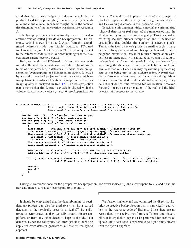

1477 Kachelrieß, Knaup, and Bockenbach: Hyperfast backprojection 1477

stand that the distance weight can always be split into aproduct of a detector preweighing function that only dependson u and v and a voxel-dependent weight that is the same asthe denominator of the perspective transform, see AppendixA.

The backprojection integral is usually realized in a dis-cretized version called pixel-driven backprojection. Our ref-erence code is shown in listing 2. Apart from this unopti-mized reference code our highly optimized PC-basedimplementation �pure C++, coded in 2001� that is equivalentto the reference code is used to benchmark against the newcell-based parallel backprojection.

Both, our optimized PC-based code and the new opti-mized cell-based implementation are hybrid algorithms interms of first performing a detector alignment, based on up-sampling �oversampling� and bilinear interpolation, followedby a voxel-driven backprojection based on nearest neighborinterpolation �a similar rectification technique is used and itsimage quality is analyzed in Ref. 17�. The backprojectionpart assumes that the detector’s � axis is aligned with the

volume’s x axis which yields c00=c20=0 �see Appendix B for

Medical Physics, Vol. 34, No. 4, April 2007

details�. The optimized implementations take advantage ofthis fact to speed up the code by reordering the nested loopsand by avoiding divisions in the innermost loop.

To achieve this alignment �ideal detector� the original data�physical detector or real detector� are transformed into theideal geometry as the first processing step. This real-to-idealrebinning includes bilinear interpolation and it includes anupsampling that doubles the number of detector pixels.Thereby, the ideal detector’s pixels are small enough to carryout the subsequent voxel-driven backprojection with nearestneighbor interpolation instead of bilinear interpolation with-out loss in image quality. It should be noted that this kind ofreal-to-ideal transform is also needed to align the detector’s uaxis along the direction of convolution before convolutioncan be carried out. Hence one may regard this preprocessingstep as not being part of the backprojection. Nevertheless,the performance values measured for our hybrid algorithmsinclude the time needed for the real-to-ideal rebinning. Theydo not include the time required for convolution, however.Figure 2 illustrates the orientation of the real and the ideal

detector with respect to the volume.

Listing 2: Reference code for the perspective backprojection. The voxel indices i, j and k correspond to x, y and z and theraw data indices l, m and n correspond to v, u and �.

It should be emphasized that the data rebinning �or recti-fication� process can also be used to switch from curveddetectors, as they typically occur in clinical CT, from dis-torted detector arrays, as they typically occur in image am-plifiers, or from any other detector shape to the ideal flatdetector. Hence the backprojection times provided here alsoapply for other detector geometries, at least for the hybridapproach.

We further implemented and optimized the direct �nonhy-brid� perspective backprojection that is numerically equiva-lent to the reference code of listing 2. Since there are nozero-valued perspective transform coefficients and since abilinear interpolation step must be performed for each voxelupdate, this direct code is expected to be significantly slowerthan the hybrid approach.

1478 Kachelrieß, Knaup, and Bockenbach: Hyperfast backprojection 1478

Implementation

The local store limit of 256 kB per worker does not allowto simultaneously update the full volume. We rather use ahierarchical memory layout and tile the volume into smallsubvolumes of 32�32�32 voxels. Such a subvolume occu-pies half of the LS. The remaining 128 kB are used to holdthe code, the stack, to hold two raw data buffers and, in caseof the hybrid algorithm, to hold the ideal detector data thatare produced during real-to-ideal rebinning �see Fig. 3�. Onlythose patches of raw data that are actually needed to back-project the current worker’s 32�32�32 subvolume areDMAed to the worker. While the worker is busy rebinningand backprojecting the first raw data buffer, the DMA of thenext raw data patch was active. Just as in the parallel back-projection case we thereby achieve to hide the DMA latencybehind the perspective backprojection process.

Again, loop unrolling techniques and instruction reorder-ing methods were employed to fully fill the execution pipe-lines while care was taken to demand for not more than the

FIG. 4. A simulated noise-free phantom consisting of fat, water, tissue and bohybrid approach. Note the narrow window width of the subtraction image: the

FIG. 3. Only small subvolumes fit into the worker. The corresponding rawdata patches are DMAed to the worker prior to real-to-ideal rebinning andbackprojection.

level of a CT image and hence negligible.

Medical Physics, Vol. 34, No. 4, April 2007

128 available registers per SPU �otherwise the compilerwould insert slow load and store instructions to accomodatedemand�.

C. Code example

To give an idea of the cell code, listing 3 shows the in-nermost loop for the direct perspective backprojection of a323 subvolume. To keep the code example short we removedthe bilinear interpolation part and only show the nearestneighbor version �that is not used for actual timing measure-ments in this paper�, for convenience. The commands usedare SPU-specific types and SPU intrinsics. Since the compu-tation of the detector indices �divisions followed by casts tointegers� is vectorized the loop index k increases by fourelements on each pass.

The corresponding LI algorithm is almost twice as longand consists of 60 lines of code. Since the loop is passedeight times, the final version that contains both vectorizationand loop unrolling and that is used for the timing measure-ments consists of 500 lines of code. For loop unrolling wedid not simply repeat the loop body eight times but we alsorescheduled the commands to account for data dependenciesand latencies. This rescheduling is shown in listing 4 whereone can see that most variables that are loaded into registersare not used before six clock cycles �lines of code� havepassed. These six clock cycles are the latency of the com-mands and correspond to the time needed until the result forthe operation is available for further use.

D. Performance assessment

The code was implemented to cope with any number ofpixels or voxels �also nonsquare images and noncubic vol-umes�, projections and pixels per projections. For the parallelbackprojection we assessed the performance of backproject-ing 512 parallel projections into an image of size 512�512.The complexity of the code is O=5123 operations. The factthat each projection consisted of 1024 channels is irrelevantto our timing measurement. In case of the cone-beam back-projection 512 projections of size 1024�1024 were back-

ontrasts of −50, 0, 50, and 1000 HU� was reconstructed using the direct andrences between the direct and the hybrid method are below the typical noise

ne �cdiffe

1479 Kachelrieß, Knaup, and Bockenbach: Hyperfast backprojection 1479

projected into a volume of size 5123. The complexity of thecone-beam backprojection code is O=5124. For both typesof algorithms the field of view �FOV� was chosen to com-pletely lie within the circular/cylindrical field of measure-ment �FOM�. The pixel or voxel size was chosen to be thedetector element size projected to the center of rotation di-vided by the square root of two.

The standard and the optimized central processing unit�CPU�-based algorithms ran on a single 3.06 GHz Xeon pro-cessor with 533 MHz front side bus while the cell-basedimplementation used a 3 GHz CBE running on a dual cellblade �Mercury Computer Systems�. For both systems we

ensured that the second CPU or the second CBE was idle

shown in Table I The LI reference algorithm is the code

Medical Physics, Vol. 34, No. 4, April 2007

during our timing measurements. The time T per slice wasmeasured using the system clock. To improve the timing ac-curacy and to overcome the granularity of the system clockwe report the average of 512 reconstructed slices. Care wastaken that no other significant CPU workload impaired ourmeasurements.

Additionally, we compute the number of CPU clockcycles per operation as C /O with C=FT being the number ofclock cycles per reconstructed image and F being the clockfrequency that equals 3.06 GHz for our PC and 3 GHz forthe cell system.

The CPU times stated below are linearly scaled from 3.06

to the 3 GHz our cell processor uses.

Listing 3: Innermost loop of the direct perspective backprojection shortened to NN interpolation. The number of voxels Kin z direction must be a multiple of four. Loop unrolling is not shown here. The comments on the right hand side are thecorresponding pseudo-code listing. Note that most variables are four vectors and operations are element wise.

III. RESULTS

A. Parallel backprojection

The timing results for a nearest neighbor �NN� and a lin-ear interpolation �LI� parallel-beam backprojection are

provided in listing 1, the NN reference code can be found bya straightforward reduction of the LI reference algorithm tonearest neighbor. The reference algorithm is PC based butnot optimized. The PC-based optimal backprojection is ahighly optimized backprojection code that has been in use by

our group since 1999. It is pure C++, contains some loop

1480 Kachelrieß, Knaup, and Bockenbach: Hyperfast backprojection 1480

unrolling but does not explicitly make use of intrinsics orassembler code. The cell-based code is also highly optimizedas detailed earlier in this paper. All algorithms are equivalentto the reference code.

updates 4 pixels� one can theoretically update 32/3 pixels,

Medical Physics, Vol. 34, No. 4, April 2007

Apparently, the CBE achieves a backprojection rate of165 fps with nearest neighbor interpolation and 126 fps withlinear interpolation. Considering that two cells are availableper blade one may backproject 330 images per second.

Listing 4: Specialization of the inner loop of listing 3 for K=32 that shows eightfold loop unrolling. The ellipses indicatethat the actual code is about six times larger. A and B denote even or odd loop index, whereas the integers running from 0 to7 denote the loop index itself.

How does our implementation compare to the theoreticalpeak performance? Theoretically, and this assumes optimaloptimization, one may not do better than updating four pixelsper step. An update step requires at least two loads, one addand one store for nearest neighbor. The add runs on the evenpipeline and can theoretically be completely hidden by thethree load/stores that execute in parallel on the odd pipeline.Per clock �we have eight workers and assumed that each step

i.e., C /O�0.093 75. Similarly, linear interpolation requiresfour load/stores and two multiply adds which means 32/4pixel updates per clock. Hence C /O�0.125 must hold. Re-garding the measured values our implementation reaches69% �NN� and 71% �LI� of the theoretical peak performance.

B. Perspective backprojection

Table II shows the timing achieved for the perspective

backprojection. It should be noted that the direct method is

1481 Kachelrieß, Knaup, and Bockenbach: Hyperfast backprojection 1481

numerically equivalent to the reference code. Due to the in-termediate resampling step, this is not exactly the case forthe hybrid approaches.

Let us again compare the performance to the theoreticaloptimum. An update step requires at least five loads, one addand one store. The add runs on the even pipeline and cantheoretically be completely hidden by the six load/stores thatexecute on the odd pipeline. This means at most 32/6 voxelupdates per clock. Hence C /O�0.187 5 must hold. Our di-rect method achieves 15.8% and the hybrid method achieves31.6% of the theoretical peak performance.

The image quality of the direct and the hybrid approach isnearly equivalent as shown in Ref. 17. To give additionalevidence, Fig. 4 shows an example of a transversal sectionthat was reconstructed with the direct approach and with thehybrid backprojection. The difference image of these noise-free data contains only values that lie below the noise valueof typical CT exams. Consequently, the images of both meth-ods can be regarded as being equivalent. The overall highimage quality achievable with the hybrid backprojection isdemonstrated in Fig. 5 These preclinical images show anin-vivo mouse scanned with a dedicated small animal imag-ing micro-CT scanner �TomoScope 30 s, VAMP GmbH, Er-langen, Germany�.

C. DMA latency

One of the most prominent features of the CBE is its fastDMA between the main memory and the worker local store.Since cell DMA works in parallel to the SPU’s commandexecution pipeline, the DMA latency may be completely hid-den for some CPU-limited problems.

TABLE I. Timing results for the parallel backprojection for one CPU or oneCBE, respectively.

NN LI

ParBackProj C /O T−1 T C /O T−1 T

PC based, reference 93.3 0.24 fps 4.1 s 118 0.19 fps 5.2 sPC based, optimized 1.54 14.8 fps 68 ms 2.12 10.7 fps 93 msCell based, optimized 0.14 165 fps 6.1 ms 0.18 126 fps 7.9 ms

FIG. 5. In vivo study of a mouse scanned with the TomoScope 30 s cone

reconstruction is cell based and uses our hybrid backprojection. �C=100 HU, W

Medical Physics, Vol. 34, No. 4, April 2007

To measure the DMA latency for our implementations, weperformed dummy reconstructions without DMA transfersand calculated the differences of the total backprojectiontimes to that of real backprojections. The backprojectiontimes were measured with clock-cycle precision via the so-called worker decrementer. The decrementer is a counter oneach SPU that is decremented by one at each clock cycle.Statistical errors were estimated by repeating all measure-ments five times.

Table III shows the results for the parallel backprojectionand the direct perspective backprojection of a 5123 volume,both using linear interpolation. It turned out that the DMAfraction of the total reconstruction time is about 0.57% forthe parallel backprojection and about 0.37% for the perspec-tive backprojection. As expected, there is no significant dif-ference in the latencies for the direct and the hybrid cone-beam backprojection since the same amount of data aretransferred in both cases.

IV. OTHER RECENT ATTEMPTS TO SPEED UPBACKPROJECTION

Other groups have made lots of efforts to speed up CTimage reconstruction. Although a fair and quantitative com-parison is not always possible, Table IV lists those perfor-mance figures that have been published in this millennium,including those published in this paper. Benchmarks found inolder literature are considered obsolete due to the ongoingdevelopments in computer technology.

To allow for some comparison we scale the values foundin the literature to the case of backprojecting 512 projections.For the parallel beam backprojection we scale to 512�512pixels, for the cone-beam backprojection to 512�512

TABLE II. Timing results for the perspective backprojection for one CPU orone CBE, respectively.

PerBackProj C /O T−1 T 512·T

PC based, reference 309 0.07 fps 13.6 s 1.93 hPC based, hybrid 8.58 2.66 fps 376 ms 3.21 minCell based, direct 1.19 18.8 fps 53.1 ms 27.2 sCell based, hybrid 0.59 37.6 fps 26.6 ms 13.6 s

micro-CT scanner �VAMP GmbH, Erlangen, Germany�. The Feldkamp

-beam =750 HU�.

1482 Kachelrieß, Knaup, and Bockenbach: Hyperfast backprojection 1482

�512 voxels. The projection size itself is considered irrel-evant. For PC-based implementations the CPU clock rate isscaled to 3.0 GHz. This assumption is quite optimistic sincebackprojection is usually limited by memory latency andmemory speed has not increased that significantly during thelast years. Especially for older experiments that have been

TABLE III. DMA latencies for the parallel backprojecperspective backprojection of a 5123 volume. DMAvolume flow from worker to manager. The statisticalthus shown as zero.

Cell-based Without DMA

ParBackProj �4047±0� msPerBackProj, direct �27 096±1� msPerBackProj, hybrid �13 526±1� ms

TABLE IV. Top: Parallel backprojection performancvalues have been scaled to 512 projections and 5122

further scaled to a single processing unit, i.e., to oneand to 3 GHz in the case of CPU-based algorithms. Tand the type of arithmethic used: f�number of bits dstands for integer �fixed point� arithmetics.

Type

Leeser et al.a LI /i09LI /i09

Schiwietz et al.b LI /f32LI /?

Xue et al.c ? /f32? /i32? /i32? /i16

Kachelrieß et al. �this work� NN /f32LI /f32

NN /f32LI /f32

Wiesentd LI /f32Yu et al.e ? /?Goddard, Trepanierf LI /i16Xu and Muelleg LI /f32

LI /f32Kole and Beekmanh NN /?

LI /?Horneggeri NN/f32Mueller and Xuj ? /f32

? /f32? /i16

Riddell and Troussetk LI /?Kachelrieß et al. �this work� LI /f32

LI /f32LI /f32

aReference 25.bReference 26.cReference 27.dReference 28.eReference 29.f

References 30–32.

Medical Physics, Vol. 34, No. 4, April 2007

carried out on slow CPUs, this scaling will overestimate theactual performance that could be achieved with the samealgorithm on modern CPUs. Note that in most cases compar-ing the cost-to-performance ratio would be more adequatethan just comparing performance. However, there are no re-liable cost figures available to us.

�with linear interpolation� and the direct and hybridraw data flow from manager to worker. DMA put:for the parallel backprojection is below 0.1 ms and

MA get DMA put Total

6±0� ms �7±0� ms �4070±0� ms±10� ms �6±1� ms �27 196±12� ms±10� ms �6±1� ms �13 625±12� ms

ttom: perspective backprojection performance. Allls and to 5123 voxels, respectively. All values wereone FPGA, one GPU and to one CBE, respectively,

pe column specifies the interpolation type, NN or LI,s floating point arithmethics while i+number of bits

are Time Comment

U 4.66 sA 125 ms

U 22.6 s Includes FFTU 176 ms Includes FFTU 7.13 sA 273 ms

U 295 msU 143 msU 68 msU 93 msE 6.1 msE 7.9 msU 10.0 min Includes convolutionU 8.51 min Includes convolutionA 66.0 s Detector � rotation axis

U 7.57 hU 34 minU 17.3 minU 25.8 minE 1.99 min SimulationU 1.28 h Includes convolutionU 17.9 min Includes convolutionU 3.84 min Includes convolutionU 9.15 min HybridU 3.21 min HybridE 27.2 s DirectE 13.6 s Hybrid

gReference 33.hReference 34.iReference 35.jReference 36.kReference 17.

tionget:error

D

�1�94�93

e. Bopixe

CPU,he tyenote

Hardw

CPFPGCPGPCP

FPGGPGPCPCPCBCBCPCP

FPGCPGPGPGPCBCPGPGPCPCPCBCB

1483 Kachelrieß, Knaup, and Bockenbach: Hyperfast backprojection 1483

A further complication regarding the cone-beam back-projection algorithms is given by the fact that the underlyingassumptions are different from publication to publication andit is not always clear whether all assumptions are preciselystated in the paper. One example are assumptions about thedetector alignment. Another assumption that is sometimesmade is that the scanner performs an exact rotation. In thiscase the perspective coefficients are not independent but canbe transformed into each other using a rotation matrix. Thisallows to use the resulting symmetries and thereby speed upthe reconstruction process.

We further want to point to the fact that there are signifi-cant differences whether the reconstructed FOV is cuboid orcylindrical �or even spherical�. A cylindrical FOV containsonly � /4�79% of the voxels that are contained in the en-closing cuboid. This adds another 21% uncertainty to thevalues found in the literature if the FOV shape is not dis-closed or if voxels outside the FOM are not backprojected.Similarly, the volume ratio between a spherical FOV and itsenclosing cube is � /6�52%.

Divide-and-conquer-type backprojection, such as Fourier-based image reconstruction,18–20 hierarchicalbackprojection21 or the link method,22 for example, is ofcompletely different type than the standard backprojectionalgorithms discussed here and therefore not included in ourcomparison. It should be noted that these methods have thepotential to increase reconstruction speed by a factorcN / ln N with c being some �sometimes rather small� con-stant. Except maybe for Fourier reconstruction there is nohighly optimized implementation that can really competewith the standard backprojection performance values listedhere. Further, some of these divide-and-conquer conceptswork well in 2D but become difficult or impossible in thecone-beam case. For example, Fourier reconstruction in 3Donly works when the complete Radon data are available.23

Last but not least, they often suffer from a trade-off betweenreconstruction speed and reconstruction accuracy, except forthe Fourier-based algorithms.

We also did not include the interesting distance-drivenbackprojection algorithm proposed in reference.24 Althoughthe authors claim significant speed-ups relative to their pixel-driven backprojection implementation, their approach is notfully optimized. Hence the achievable timing cannot be reli-ably determined from the paper.

A. Parallel backprojection

Leeser et al. published an field programmable gate array�FPGA�-driven parallel beam backprojection.25 Using fixedpoint arithmetic with 9 bits they can backproject 1024 pro-jections into a 5122 image in 0.25 s using “16-way parallelprocessing.” A great deal of their work has to do with bitreduction which always means a loss of image quality, how-ever. They assume 12 bit input data �which is not sufficientfor clinical CT where the data are acquired with at least 20bits�. They compare their results to a 1 GHz CPU-based ver-

sion that needs 28 s for the 1024 projections.

Medical Physics, Vol. 34, No. 4, April 2007

Schiwietz et al. compare CPU-based with graphical pro-cessing unit �GPU�-based magnetic resonance imagereconstruction.26 Since they start in Fourier domain theircode includes the inverse fast Fourier transform �FFT� toobtain data ready for backprojection. They use a 3 GHz CPUand an ATI Radeon X1800 XT GPU. The reconstruction ofthree 2562 images from 504 projections requires 16.7 s onthe CPU and 130 ms on the GPU. Normalizing this to one5122 image and 512 projection yields 22.6 s and 176 ms,respectively.

Xue and co-authors compared CPU with GPU and withFPGA performance for a parallel beam backprojection from165 projections into a 2562 image.27 Their PC runs at3.4 GHz and they compare the ATI X700 Pro and the NVidiaGF7800 GPU whereby the Nvidia greatly outperforms theATI GPU. The CPU code uses floating point arithmetics andan image is backprojected in 507 ms. The FPGA uses fixedpoint arithmetics with 32 bit precision and does the same jobin 22 ms. The GPU �Nvidia� with 32 bit fixed point arithmet-ics performs in 23.8 ms and with 16 bit it does the back-projection in 11.5 ms. Scaling these values to 512 projec-tions, 5122 image pixels and to 3.0 GHz yields 7.13 s �CPU�,273 ms �FPGA�, 295 ms �GPU, 32 bit� and 143 ms �GPU,16 bit�, respectively, for one image.

B. Perspective backprojection

Wiesent et al. use a dual Pentium III Xeon 550 MHzCPU.28 They reconstruct 2563 voxels from 100 projections inabout 40 s. In terms of the 5124 operations at 3 GHz and asingle CPU this scales to 10.0 min.

Yu et al. provide a PC-based implementation.29 On a500 MHz Pentium III CPU they can reconstruct a 5123 vol-ume from 288 projections within 15.03 min. They use aspherical FOV and do not backproject voxels outside thissphere. Scaled to 3 GHz, to 512 projections and to a cubicFOV this becomes 8.51 min whereby we believe that thisscaling yields a far too optimistic value since memory speeddid not improve the same way as the CPU clock rates did.Their code utilizes single instruction multiple data instruc-tions.

Goddard and Trepanier present an FPGA-driven recon-struction �which includes convolution� that can reconstruct a5123 volume from 300 projections between 15 and38.7 s.30–32 The range of values corresponds to using one ormore FPGAs. Since the convolution process was completelyhidden behind the backprojection, the reconstruction timesalso correspond to the backprojection performance. Scalingthe 38.7 s �one FPGA� to the 512 projections used here weobtain a performance of 66.0 s. Among other assumptionsthe algorithm assumes one detector axis to be parallel to therotation axis, the center of rotation to be the center of thecubic volume, and the distances of the focal spot to the iso-center and to the detector to be constant. The first assumptionimplies that their backprojection matrix is of the same type

as for our hybrid approach. The real-to-ideal rebinning is not

1484 Kachelrieß, Knaup, and Bockenbach: Hyperfast backprojection 1484

mentioned and probably not included in their experiment.The other assumptions imply that the perspective coefficientscij are generated by a rotation matrix.

Xu and Mueller published on GPU-based imagereconstruction.33 They compare a “fairly optimized CPUimplementation” with the GPU-based approach they pro-pose. The PC runs on 2.66 GHz and the GPU is an NvidiaFX 5900. Their backprojection �LI� requires 75 s for thefairly optimized CPU algorithm and 5 s for the GPU codewhen a volume of 1283 and 80 projections are used. In termsof our 5124 problem at 3.0 GHz these values become 7.57 hfor the PC and 34 min for the GPU, respectively.

Kole and Beekman recently optimized a statistical imagereconstruction algorithm to run on a GPU.34 Each iterationconsists of one forward and two backprojection steps. Sincethe forward projection is of about the same speed as thebackprojection, we may divide their performance values bythree to estimate the GPU performance of a perspectivebackprojection. They cite a speed of 195 s for NN and of290 s for LI for one iteration consisting of 256 projectionsand a 2563 volume. The time needed for a backprojection ofthe 5124 problem will be about 17.3 min for the nearestneighbor backprojection and about 25.8 min for the linearinterpolation version.

Hornegger recently presented a backprojection code forthe cell processor that was tested on a cell simulator and noton a real cell system.35 They show that six projections/s canbe backprojected �NN� on a 5123 volume using a dual cell�16 SPUs� running with 2.1 GHz and speculate that the codecan be further sped up by a factor of 5. Scaling their value to512 projections, 3.0 GHz and 1 CBE yields 1.99 min for thecomplete volume.

Lately, Mueller and Xu published new results on GPU-based CT image reconstruction.36 Since the problem of float-ing point arithmetics on GPUs seems not yet to be solvedthey find integer arithmetics very useful to speed up the pro-cess although image quality becomes inferior. Depending onwhat arithmetic is used, the timing for a 2563 volume and160 projections achieved on an Nvidia 7800 FX GPU rangesfrom everything between 1.9 and 42 s. Adequate images areprovided by their “dual-pass” approach that allows for 16 bitaccuracy and finishes in 9 s. Full floating point accuracy re-quires 42 s on the GPU. Their PC-based implementationneeds 180 s for the same task in full floating point accuracy�CPU and bus clock frequencies are not stated�. Normalizingtheir values to 5124 yields 3.84 min �16 bit integer� and17.9 min �single precision float� for the GPU and 1.28 h forthe CPU. It should be noted that these values include theconvolution step which typically makes up about 10% of thereconstruction time if it cannot be hidden behind the back-projection by using a parallel thread.

Riddell and Trousset implemented a rectification-basedperspective backprojection on a 3.4 GHz Pentium 4 CPU.17

Their code uses the decomposition given in Appendix B andtherefore is a hybrid approach. In contrast to our cell-basedhybrid algorithm that first performs the alignment A fol-lowed by the backprojection B ·C Riddell and Trousset per-

form the “rectification” A ·B followed by the backprojection

Medical Physics, Vol. 34, No. 4, April 2007

C. The authors state that backprojecting 148 projections intoa cylinder of 512 voxels height and diameter takes 110 s.Scaling this to our 5124 problem and to 3.0 GHz we find thattheir code takes 9.15 min.

V. DISCUSSION

The cell broadband engine enables very fast backprojec-tion on a general purpose hardware. The parallel backprojec-tion performance allows to generate 330 images �5122 pixels,512 projections�/s on a dual cell board. For the cone-beambackprojection one may generate a complete volume �5123

voxels, 512 projections� in 6.8 s. �Convolution of 512 pro-jections of size 1024�1024 with a 2047-element kernel runsin 0.2 s on the dual cell blade and is therefore negligiblecompared to the backprojection step.�

Considering that typical scan times are in the same order�at least for flat-panel detector-based CT� one can potentiallyachieve real-time imaging at full spatial resolution. Besidesits very high performance, probably the most significant ad-vantage of the CBE over other hardware-based accelerationapproaches is its versatility. FPGA-, application specific in-tegrated circuit �ASIC�-, or GPU-based solutions are usuallylimited to certain functionality. The cell processor, in con-trast, is a general purpose hardware that can be used for allkinds of tasks ranging from data preprocessing, image recon-struction, image display, volume rendering to more compli-cated issues such as done and scatter calculation. Its highperformance may even leverage completely new applicationsor may help to bring other, low performance approaches intoclinical routine, such as iterative or statistical CT image re-construction, for example.

APPENDIX A: DISTANCE WEIGHTING

Distance weighting means multiplying each voxel’s up-date value during backprojection prior to accumulation by afunction Wn�r−s� where n is some power, r is the voxellocation, s is the source or vertex position of the perspectivetransform, and where W is a homogeneous function of de-gree one.

We will now show that significant parts of this voxel-based distance weighting can be reorganized such that a de-tector pixel-based weighting can be performed.

Let q=r−s, define the perspective projection of point rwith vertex s as

u =c0 · q

c2 · qand v =

c1 · q

c2 · qwith ci = ci0

ci1

ci2

and verify by expansion that

q =c0 � c1 + uc1 � c2 + vc2 � c0

�c0 � c1� · c2�c2 · q� .

Obviously, q is decomposed into a function of u and v andinto a factor that corresponds to the denominator of the per-

spective transform, i.e., q=��u ,v��c2 ·q�, is valid. Hence

1485 Kachelrieß, Knaup, and Bockenbach: Hyperfast backprojection 1485

W�q� = W���u,v��c2 · q�� = W���u,v���c2 · q�

= W�u,v��c2 · q�

is a decomposition of the distance weight into a product ofdetector weight and voxel weight. The detector weight mustbe applied to the raw data before they are passed to thebackprojecting function. The latter is of type �c2 ·q� and isthe denomi of the perspective transform which is computedduring perspective backprojection anyway.

APPENDIX B: DECOMPOSITION OF THEPERSPECTIVE TRANSFORM

Using homogeneous coordinates the 3D perspective trans-form, that defines the backprojection geometry, can be writ-ten as the 3�4 matrix

Corig = c00 c01 c02 c03

c10 c11 c12 c13

c20 c21 c22 c23 .

Corig may be decomposed into a product of two 3�3detector-to-detector perspective transform matrices A and Band a new 3�4 perspective backprojection matrix C

A · B · C Corig. �B1�

Each of the matrices A and B defines a 2D perspective trans-form and may be realized by rebinning the detector data. Thematrix C defines a 3D perspective transform between thevolume and the detector. A is designed to align the detector’scoordinate axes with an arbitrary vector t on the one handand with the volume’s x axis on the other hand. B furtheraligns the detector such that its u axis is parallel to the vol-ume’s y axis and that its v axis remains parallel to the vol-ume’s x axis.

The new transform matrices are given by

A = c0 · t �v1,w2� 0

c1 · t �u2,w1� 0

c2 · t �u1,v2� ,

B = w2 0 0

�t2,w0� �t1,w2� 0

− t2 0 �t1,w2� ,

C = 0 − w2 w1 �s1,w2�− w2 0 w0 �s0,w2�

0 0 − 1 s2

and the �irrelevant� constant of proportionality of the righthand side of Eq. �B1� is given by �t2 ,w1� w2. Here, we usethe commutator �ui ,v j�=uiv j −ujvi, the scale factor �

= c0 · �c1�c2�, and the coefficient vector

Medical Physics, Vol. 34, No. 4, April 2007

ci = ci0

ci1

ci2

for abbreviation. The vectors s, t, u, v and w, whose com-ponents are denoted as s0 ,s1 , . . . , can be identified with thesource �or vertex� position, the direction of convolution, thevectors spanning the detector, and the vector connecting thedetector origin with the vertex, respectively. Whereas t isarbitrary and usually depends on the tangent of the scan tra-jectory, the others are given by

s = − c00 c01 c02

c10 c11 c12

c20 c21 c22

−1

· c03

c13

c23 and

u = c1 � c2/

v = c2 � c0/

w = c0 � c1/

.

There are two advantages of this kind of decomposition.One is that convolution must usually be carried out along acertain direction t that corresponds to the tangent t=s���� ofthe source trajectory s���. To avoid convolving across detec-tor rows, which would be highly inefficient, the detectormust be rebinned using the transform A. Only then, convo-lution can be done along the detector’s u axis for each de-tector row v separately.

The second advantage of the detector alignment is thatthere are a number of zeroes introduced into the backprojec-tion matrix. These zeroes help to improve the backprojectionspeed. Depending on whether there is no detector alignmentat all, only the convolution alignment A or both alignmentsteps A and B are performed the final backprojection matrixwill become one of

Cbp= A · B · C Corig

Cbp= B · C

Cbp= C .

The zero entries of Cbp and the detector orientation areillustrated in Table V. Note that whenever one desires full

TABLE V. Possible alignment steps of the projection data to allow for con-volution along t and to introduce a number of zeroes in the backprojectionmatrix. Our hybrid code versions perform the convolution alignment A,assume the convolution to be performed elsewhere, and finally use the 3Dperspective transform matrix Cbp=B ·C for backprojection.

Detector A�from scanner�

Detector B�convolution�

Detector C�backprojection�

u axis u t yv axis v x xCbp � · · · ·

· · · ·

· · · · � �0 · · ·

· · · ·

0 · · · � �0 · · ·

· 0 · ·

0 0 · · �� � �

A ·B ·C B ·C C

alignment but does not need the intermediate convolution

1486 Kachelrieß, Knaup, and Bockenbach: Hyperfast backprojection 1486

step, one may perform transforms A and B simultaneouslyby using the 3�3 detector-to-detector transform matrix A ·Binstead.

It must be emphasized that the decomposition shown herecorresponds to a particular detector and volume orientation.Aligning the detector parallel to the x and y axis of the vol-ume is reasonable only when the projection is oriented moreor less along the z direction. For other projections detectoralignments along the x-z plane or along the y-z plane arerequired. These situations can be easily handled by swappingthe corresponding rows of Corig.

a�Electronic mail: marc.kachelriess@imp.uni-erlangen.de1H. P. Hofstee, “Power efficient processor architecture and the cell proces-sor,” Proceedings of the 11th International Symposium on High-Performance Computer Architecture, 12–16 February 2005, San Fran-cisco, CA.

2D. Pham, S. Asano, M. Bolliger, M. N. Day, H. P. Hofstee, C. Johns, J.Kahle, A. Kameyama, J. Keaty, Y. Masubuchi, M. Riley, D. Shippy, D.Stasiak, M. Suzuoki, M. Wang, J. Warnock, S. Weitzel, D. Wendel, T.Yamazaki, and K. Yazawa, “The design and implementation of a first-generation cell processor,” IEEE International Solid-State Circuits Con-ference, pp. 184–185, 6–10 February 2005, San Francisco, CA.

3B. Flachs, S. Asano, S. H. Dhong, H. P. Hofstee, G. Gervais, R. Kim, T.Le, P. Liu, J. Leenstra, J. Liberty, B. Michael, H. Oh, S. M. Mueller, O.Takahashi, A. Hatakeyama, Y. Watanabe, and N. Yano, “A streamingprocessing unit for a cell processor,” IEEE International Solid-State Cir-cuits Conference, pp. 134–135, 6–10 February 2005, San Francisco, CA.

4W. A. Kalender, Computed Tomography, 2nd ed. �Wiley, New York,2005�.

5Gabor T. Herman, Image Reconstruction from Projections: The Funda-mentals of Computerized Tomography (Computer Science and AppliedMathematics) �Academic, New York, 1980�.

6H. H. Barrett and W. Swindell, Radiological Imaging �Academic, NewYork, 1981�.

7A. C. Kak and M. Slaney, Principles of Computerized Tomographic Im-aging �SIAM, Philadelphia, 1988�.

8F. Natterer, The Mathematics of Computerized Tomography �Teubner,Stuttgart, 1989�.

9L. A. Shepp and B. F. Logan, “The Fourier reconstruction of head sec-tion,” IEEE Trans. Nucl. Sci. 21, 21–43 �1974�.

10L. A. Feldkamp, L. C. Davis, and J. W. Kress, “Practical cone-beamalgorithm,” J. Opt. Soc. Am. A 1�6�, 612–619 �1984�.

11M. Kachelrieß, S. Schaller, and W. A. Kalender, “Advanced single-slicerebinning in cone-beam spiral CT,” Med. Phys. 27�4�, 754–772 �2000�.

12L. M. Chen, D. J. Heuscher, and Y. Liang, “Oblique surface reconstruc-tion to approximate cone-beam helical data in multislice CT,” Proc. SPIE4123, 279–284 �2000�.

13S. Schaller, K. Stierstorfer, H. Bruder, M. Kachelrieß, and T. Flohr,“Novel approximate approach for high-quality image reconstruction inhelical cone beam CT at arbitrary pitch,” SPIE Medical Imaging Confer-ence Proc. 4322, 113–127 �2001�.

14M. Kachelrieß, T. Fuchs, S. Schaller, and W. A. Kalender, “Advancedsingle-slice rebinning for tilted spiral cone-beam CT,” Med. Phys. 28�6�,1033–1041 �2001�.

15

K. Stierstorfer, T. Flohr, and H. Bruder, “Segmented multiple plane

Medical Physics, Vol. 34, No. 4, April 2007

reconstruction—a novel approximate reconstruction for multi-slice spiralCT,” Phys. Med. Biol. 47, 2571–2851 �2002�.

16M. Knaup, W. A. Kalender, and M. Kachelrieß, “Statistical cone-beamCT image reconstruction using the cell broadband engine,” IEEE MedicalImaging Conference Record 2006, Oct 29–Nov 4, San Diego, CA, M11-422, pp. 2837–2840.

17C. Riddell and Y. Trousset, “Rectification for cone-beam projection andbackprojection,” IEEE Trans. Med. Imaging 25�7�, 950–962 �2006�.

18H. Stark, J. W. Woods, I. Paul, and R. Hingorani, “An investigation ofcomputerized tomography by direct Fourier inversion and optimum inter-polation,” IEEE Trans. Biomed. Eng. 28�7�, 496–505 �1981�.

19H. Schomberg and J. Timmer, “The gridding method for image recon-struction by Fourier transformation,” IEEE Trans. Med. Imaging 14�3�,596–607 �1995�.

20S. Schaller, T. Flohr, and P. Steffen, “An efficient Fourier method in 3Dreconstruction from cone-beam data,” IEEE Trans. Med. Imaging 17,244–250 �1998�.

21S. Basu and Y. Bresler, “An O�N2 log N� filtered backprojection recon-struction algorithm for tomography,” IEEE Trans. Med. Imaging 9�10, �1760–1773 �2000�.

22P. E. Danielsson and M. Ingerhed, “Backprojection in O�N2 log N� time,”IEEE Nucl. Sc. Symp. Rec. 2, 1279–1283 �1998�.

23C. Axelsson and P. E. Danielsson, “Three-dimensional reconstructionfrom cone-beam data in O�N3 log N� time,” Phys. Med. Biol. 39�3� 447–491 �1994�.

24B. De Man and S. Basu, “Distance-driven projection and backprojectionin three dimensions,” Phys. Med. Biol. 49, 2463–2475 �2004�.

25M. Leeser, S. Coric, E. Miller, H. Yu, and M. Trepanier, “Parallel-beambackprojection: An FPGA implementation optimized for medical imag-ing,” Proceedings of the Tenth Int. Symposium on FPGA, Monterey, CA,217–226, February �2002�.

26T. Schiwietz, T.-C. Chang, P. Speier, and R. Westermann, “MR imagereconstruction using the GPU,” Proc. SPIE 6142, 1279–1290 �2006�.

27X. Xue, A. Cheryauka, and D. Tubbs, “Acceleration of fluoro-CT recon-struction for a mobile C-arm on GPU and FPGA hardware: A simulationstudy,” Proc. SPIE 6142, 1494–1501 �2006�.

28K. Wiesent, K. Barth, N. Navab, P. Durlak, T. Brunner, O. Schuetz, andW. Seissler, “Enhanced 3D reconstruction algorithm for C-arm systemssuitable for interventional procedures,” IEEE Trans. Med. Imaging 19�5�,391–403 �2000�.

29R. Yu, R. Ning, and B. Chen, “High-speed cone-beam reconstruction onPC,” Proc. SPIE 4322, 964–973 �2001�.

30M. Trepanier and I. Goddard, “Adjunct processors in embedded medicalimaging systems,” Proc. SPIE 4681, 416–424 �2002�.

31I. Goddard and M. Trepanier, “High-speed cone-beam reconstruction: Anembedded systems approach,” Proc. SPIE 4681, 483–491 �2002�.

32I. Goddard and M. Trepanier, “The role of FPGA-based processing inmedical imaging,” VMEbus systems �2003�.

33F. Xu, and K. Mueller, “Accelerating popular tomographic reconstructionalgorithms on commodity PC graphics hardware,” IEEE Trans. Nucl. Sci.52�3�, 654–663 �2005�.

34J. S. Kole and F. J. Beekman, “Evaluation of accelerated iterative x-rayCT image reconstruction using floating point graphics hardware,” Phys.Med. Biol. 51, 875–889 �2006�.

35J. Hornegger, “Moscow-Bavarian joint advanced student school” �2006�.www5.informatik.uni-erlangen.de/Lehre/WS0506/MB-JASS06/

36K. Mueller and F. Xu, “Practical considerations for GPU-accelerated CT,”IEEE International Symposium on Biomedical Imaging, pp. 1184–1187,

April �2006�, Arlington, Virginia.