hyperelastic structural fuses for improved …
TRANSCRIPT

University of Nebraska - LincolnDigitalCommons@University of Nebraska - LincolnCivil Engineering Theses, Dissertations, andStudent Research Civil Engineering
Summer 7-28-2017
HYPERELASTIC STRUCTURAL FUSES FORIMPROVED EARTHQUAKE RESILIENCE OFSTEEL CONCENTRICALLY-BRACEDBUILDINGSFrancys López-MosqueraUniversity of Nebraska - Lincoln, [email protected]
Follow this and additional works at: http://digitalcommons.unl.edu/civilengdiss
Part of the Architectural Engineering Commons, and the Engineering Science and MaterialsCommons
This Article is brought to you for free and open access by the Civil Engineering at DigitalCommons@University of Nebraska - Lincoln. It has beenaccepted for inclusion in Civil Engineering Theses, Dissertations, and Student Research by an authorized administrator ofDigitalCommons@University of Nebraska - Lincoln.
López-Mosquera, Francys, "HYPERELASTIC STRUCTURAL FUSES FOR IMPROVED EARTHQUAKE RESILIENCE OFSTEEL CONCENTRICALLY-BRACED BUILDINGS" (2017). Civil Engineering Theses, Dissertations, and Student Research. 114.http://digitalcommons.unl.edu/civilengdiss/114

HYPERELASTIC STRUCTURAL FUSES FOR IMPROVED EARTHQUAKE
RESILIENCE OF STEEL CONCENTRICALLY-BRACED BUILDINGS
by
Francys López-Mosquera
A THESIS
Presented to the Faculty of
The Graduate College at the University of Nebraska
In Partial Fulfillment of Requirements
For the Degree of Master of Science
Major: Civil Engineering
Under the Supervision of Professor Joshua Steelman
Lincoln, Nebraska
August, 2017

HYPERELASTIC STRUCTURAL FUSES FOR IMPROVED EARTHQUAKE
RESILIENCE OF STEEL CONCENTRICALLY-BRACED BUILDINGS
Francys López-Mosquera, M.S.
University of Nebraska, 2017
Advisor: Joshua Steelman
Improving structural resilience (i.e., reducing service interruptions and improving
rapidity of function restoration) following extreme events is one of the primary
contemporary challenges in structural engineering. While massive casualties have
successfully been avoided through the adoption of modern building codes, the sole
codified performance objective has been limited to the life safety/collapse prevention
range of response. Christchurch, NZ, highlighted the insufficiency of this approach, with
large sections of the city nonfunctional after a major earthquake, and with subsequent
collapses induced by significant aftershocks. Engineering advances to improve building
and community resilience are necessary to mitigate hazards from becoming disasters.
This study explores the influence and potential benefits of introducing a hyperelastic 3D
printed fusing component on global performance outcomes, focusing primarily on direct
economic loss estimates. This work identifies potentially beneficial combinations of
hyperelastic component phenomenological parameters (i.e., stiffness, ductility, resisting
force), presenting the results as a performance comparison between the hyperelastic and
conventional hysteretic systems. Current 3D printing technologies allow the easy creation
of complex geometries, hence it is expected that 3D printed steel fuses can provide a
strategically defined multi-linear hyperelastic constitutive response through geometric
configuration and small-scale elastic buckling. The hyperelastic component behavior

permits shared participation of mechanical and inertial effects at the global structure
level, while also achieving self-centering after extreme loading has concluded.
Additionally, the lack of residual drift combined with the lack of significant structural
damage will permit continued occupation with minimal functional disruption.

iii
ACKNOWLEDGEMENTS
Foremost, I want to thank my advisor, Dr. Joshua Steelman, for his commitment, patience
and constant support through the learning process of this master thesis. Thank you for the
stimulating discussions, and I feel honored to have had the opportunity to work with such a
genuine professor.
I would like to thank my fellow graduated students, Pranav Shakya, Ahmed Rageh, Fayaz
Sofi, Steven Stauffer, Linh Abdulrahman, and Cesar Gomez, who have contributed to building
my body of knowledge through this challenging experience at UNL. I will never forget the
sleepless nights working together before deadlines, but overall I will always remember your
friendship and advice.
I want to express my gratitude to my committee members Dr. Christine Wittich and Dr.
Ronald Faller for sharing their time and expertise in my advisory committee to strengthen this
work.
I would like to acknowledge Amber Hadenfeldt for her responsiveness and guidance in
editing this thesis. All your suggestions and comments enriched this work tremendously.
I would like to thank Fulbright Colombia and the UNL Civil Engineering department for
funding me through this program.
Lastly, and most importantly, I want to thank God and my loved ones for being there for
me even when it seemed I was not there for you. Your continuous encouragement kept this boat
afloat through the worst storms.

iv
TABLE OF CONTENTS
CHAPTER 1. INTRODUCTION ............................................................................................. 1
CHAPTER 2. LITERATURE REVIEW .................................................................................. 9
2.1. Fuses in Braced Frames.................................................................................................... 9
2.2. State of the Art in Resilient Structural Systems ............................................................. 11
2.2.1. “Development of a ratcheting, tension-only fuse mechanism for seismic energy
dissipation” (2015) .............................................................................................................................. 12
2.2.2. “Optimal Seismic Performance of Friction Energy Dissipating Devices” (2008) ................. 13
2.2.3. “Shake table test and numerical study of self-centering steel frame with SMA braces”
(2016) 14
2.2.4. “Analytical Response and Design of Buildings with Metallic Structural Fuses. I” (2009) ... 15
2.2.5. “Seismic Response of Multistory Buildings with Self-Centering Energy Dissipative Steel
Braces” (2008) ..................................................................................................................................... 16
2.2.6. “Self-Centering Energy-Dissipative (SCED) Brace: Overview of Recent Developments and
Potential Applications for Tall Buildings” (2014) ................................................................................ 17
2.2.7. “Seismic Assessment of Concentrically-braced Steel Frames with Shape Memory Alloy
Braces” (2007) ..................................................................................................................................... 17
2.2.8. “An innovative seismic bracing system based on a shape memory alloy ring,” (2016). .... 18
2.2.9. “Seismic resistant rocking coupled walls with innovative Resilient Slip Friction (RSF) joints”
(2017) 19
2.3. Earthquake Loss Assessment ......................................................................................... 20
2.3.1. “Lessons from the February 22nd Christchurch Earthquake” (2012) ................................. 21
2.3.2. “Steel Building Damage from The Christchurch Earthquake Series of 2010 And 2011”
(2012) 21
2.3.3. “Estimation of Seismic Acceleration Demands in Building Components” (2004) .............. 23
CHAPTER 3. OBJECTIVES AND SCOPE........................................................................... 25
3.1. Objectives ....................................................................................................................... 25
3.2. Scope ............................................................................................................................. 25
CHAPTER 4. METHODOLOGY .......................................................................................... 27
4.1. Prototype Buildings ........................................................................................................ 27
4.2. Design of Prototype Buildings ....................................................................................... 29
4.2.1. Equivalent Lateral Force (ELF) ............................................................................................. 30
4.2.2. Response Modification Coefficient R. ................................................................................. 31
4.3. Prototype Buildings Simplification to Single Degree of Freedom (SDOF) Systems .... 35

v
4.4. Ground Motions ............................................................................................................. 37
4.5. Earthquake Estimates of Direct Physical Building Damage .......................................... 41
4.5.1. Fragility Curves .................................................................................................................... 41
4.6. Parametrization............................................................................................................... 50
4.6.1. Sensitivity Analysis. ............................................................................................................. 51
CHAPTER 5. RESULTS ........................................................................................................ 54
5.1. Overview ........................................................................................................................ 54
5.2. Evaluation of Bilinear Hyperelastic Models .................................................................. 55
5.2.1. Bilinear, 3-Story Building, Low-Ductility (CASE D) ............................................................... 56
5.2.2. Bilinear, 1-story Building, Low-Ductility (CASE C) ............................................................... 58
5.2.3. Bilinear, 3-story Building, High Ductility (CASE B) ............................................................... 59
5.2.4. Bilinear, 1-Story Building, High Ductility (Case A). .............................................................. 61
5.2.5. Summary and Loss Assessment Estimates for Bilinear Hyperelastic Models. .................... 62
5.3. Trilinear Hyperelastic Evaluations ................................................................................. 63
5.3.1. Trilinear, 3-Story Building, Low-Ductility (CASE D) ............................................................. 65
5.3.2. Trilinear, 1-Story Building, Low-Ductility (CASE C) .............................................................. 73
5.3.3. Trilinear, 3-Story Building, High Ductility (CASE B) ............................................................. 79
5.3.4. Trilinear, 1-Story Building, High Ductility (Case A). ............................................................. 84
CHAPTER 6. CONCLUSIONS ............................................................................................. 89
6.1. Case Specific .................................................................................................................. 89
6.1.1. CASE D. (3 stories, R=3.1/4) ................................................................................................ 89
6.1.2. CASE C (1 story, R=3.1/4) .................................................................................................... 89
6.1.3. CASE B (3 stories, R=6) ........................................................................................................ 90
6.1.4. CASE A (1-Story Building, High Ductility)............................................................................. 90
6.2. General ........................................................................................................................... 91
6.3. Future Research Needs and Opportunities ..................................................................... 92
CHAPTER 7. REFERENCES ................................................................................................ 94

vi
LIST OF FIGURES FIGURE 1. IDEALIZED HYPERELASTIC BRACED FRAME...................................................................... 4 FIGURE 2. IDEALIZED HYPERELASTIC STRUCTURAL FUSE. RIGHT: GENERAL DESCRIPTION; LEFT:
SKETCH OF THE INTERNAL BUCKLING MECHANISM. ................................................................. 5 FIGURE 3. 3D RENDERING OF IDEALIZED HYPERELASTIC FUSE. ....................................................... 6 FIGURE 4. FORCE-DISPLACEMENT CURVE OF THE HYPERELASTIC SYSTEM. ..................................... 7 FIGURE 5. HYSTERETIC BEHAVIOR OF CONVENTIONAL STRUCTURAL SYSTEMS: (A) STEEL MOMENT
RESISTING FRAME; (B) SINGLE STEEL BRACE; (C) CONCRETE SHEAR WALL. (NATHAN
CHANCELLOR ET AL. 2014) .................................................................................................... 10
FIGURE 6. (A) RATCHET MECHANISM ASSEMBLY; (B) FORCE DISPLACEMENT HYSTERESIS (COOK ET
AL. 2015). .............................................................................................................................. 12 FIGURE 7. RIGHT: SCHEMATIC DIAGRAM OF FOUR-STORY BUILDING WITH FRICTION DEVICES
(DIMOVA ET AL. 1995), LEFT: DRY FRICTION MODELS (A) COULOMB FRICTION MODEL (B)
REALISTIC FRICTION MODEL (PATRO AND SINHA, 2008). ..................................................... 13
FIGURE 8. SMA-BASED DAMPER: (A) CONFIGURATION OF SMA DAMPER; (B) DEFORMATION UNDER
TENSION AND COMPRESSION; AND (C) IDEALIZED FLAG-SHAPED HYSTERESIS (QIU AND ZHU
2017B) ................................................................................................................................... 14 FIGURE 9. (A) SAMPLE MODEL OF AN SDOF SYSTEM WITH METALLIC FUSES; (B) GENERAL
PUSHOVER CURVE .................................................................................................................. 15
FIGURE 10. BRACE HYSTERETIC RESPONSE: (A) CONVENTIONAL BRACE; (B) BUCKLING RESTRAINED
BRACE; AND (C) SCED BRACE. (TREMBLAY ET AL. 2008) ..................................................... 16
FIGURE 11. POTENTIAL TALL BUILDING CONFIGURATIONS USING SCED BRACES PRESENTED BY
EROCHKO AND CHRISTOPOULOS N.D. .................................................................................... 17
FIGURE 12. RIGHT: EXPERIMENTAL SETUP: (A) LOADING TEST FRAME, (B) SMA RING AND STEEL
CONNECTIONS, (C) TURNBUCKLE AND CUSTOM-MADE LOAD CELL, AND (D) PAD-EYE
CONNECTION AND LVDT. LEFT: A CROSS-BRACED SYSTEM BASED ON AN SMA RING (GAO ET
AL. 2016) ............................................................................................................................... 18 FIGURE 13. RIGHT: RSF JOINT: A) CAP PLATES AND SLOTTED CENTER PLATES B) BELLEVILLE
SPRINGS C) HIGH STRENGTH BOLTS D) ASSEMBLY OF THE JOINT. LEFT: SCHEMATIC LOAD-
DEFORMATION LOOP FOR THE RSF JOINT. .............................................................................. 19 FIGURE 14. CHRISTCHURCH PARKING LOT [PHOTOS BY M. BRUNEAU]; (A) INELASTIC
DEFORMATIONS AT TOP LEVEL EBF; (B) FRACTURED LINK AT LOWER LEVEL EBF. (CLIFTON
ET AL. 2011)........................................................................................................................... 22
FIGURE 15. LOW‐RISE CBF PARKING GARAGE [PHOTOS BY M. BRUNEAU]. (A) BUCKLED BRACE;
(B) FRACTURED NON‐DUCTILE BRACE‐TO‐COLUMN CONNECTION (CLIFTON ET AL. 2011). .... 23 FIGURE 16. ACCELERATION-SENSITIVE NONSTRUCTURAL COMPONENTS (TAGHAVI, SHAHRAM;
MIRANDA 2004)..................................................................................................................... 23 FIGURE 17. PROTOTYPE BUILDINGS. (A) PLAN VIEW; (B) 3-STORY ELEVATION VIEW; (C) 1-STORY
ELEVATION VIEW ................................................................................................................... 29 FIGURE 18. 3D ANALYSIS MODELS; SAP2000; (A) 3-STORY; (B) 1-STORY .................................... 30 FIGURE 19. CHOPRA ILLUSTRATION FOR EFFECTIVE MODAL MASSES AND HEIGHTS (CHOPRA 2012).
............................................................................................................................................... 36 FIGURE 20. SCALING FACTORS ...................................................................................................... 39 FIGURE 21. ELASTIC SPECTRUMS OF SCALED GROUND MOTIONS ................................................. 41 FIGURE 22 HAZUS-MH EXAMPLE OF FRAGILITY CURVES FOR SLIGHT, MODERATE, EXTENSIVE
AND COMPLETE DAMAGE ...................................................................................................... 42

vii
FIGURE 23. (A) HYSTERETIC SYSTEM BEHAVIOR; (B) HYPERELASTIC SYSTEM. ............................... 50 FIGURE 24. TREND IDENTIFICATION EXAMPLE BY USING MAXIMUM RESPONSE TREND LINES
(MRTLS) ............................................................................................................................... 53 FIGURE 25. IDEALIZED FORCE- DISPLACEMENT CURVE. HYSTERETIC AND HYPERELASTIC ........... 54
FIGURE 26. FORCE-DISPLACEMENT CURVE FOR BILINEAR HYPERELASTIC SYSTEMS. ..................... 56 FIGURE 27. CASE D. DUCTILITY REQUIRED FOR A BILINEAR HYSTERETIC SYSTEM, DIFFERENT
FY/FE RATIOS. ........................................................................................................................ 57 FIGURE 28. CASE C. DUCTILITY REQUIRED FOR A BILINEAR HYSTERETIC SYSTEM, DIFFERENT FY/FE
RATIOS. .................................................................................................................................. 59
FIGURE 29. CASE B. DUCTILITY REQUIRED FOR A BILINEAR HYSTERETIC SYSTEM, DIFFERENT FY/FE
RATIOS. .................................................................................................................................. 60
FIGURE 30. CASE A. DUCTILITY REQUIRED FOR A BILINEAR HYSTERETIC SYSTEM, DIFFERENT FY/FE
RATIOS. .................................................................................................................................. 62 FIGURE 31. LOSS ASSESSMENT ESTIMATE FOR BILINEAR HYPERELASTIC MODELS. ........................ 63 FIGURE 32. DIFFERENT HYPERELASTIC CONFIGURATIONS (FORCE-DISPLACEMENT) ..................... 64
FIGURE 33. CASE D- FY/FE EQUALS 3. (A) RIGHT: Α2= [0 TO 0.25] FOR Μ=2.5; (B) LEFT: Μ = [1 TO
10] FOR Α2 [0-0.25]. ............................................................................................................... 66
FIGURE 34. CASE D- Α2=0.1; NORMALIZED REPAIR COST, DUCTILITY, AND FY/FE RATIO. .............. 68 FIGURE 35. CASE D- Α2=0.05; NORMALIZED REPAIR COST, DUCTILITY, AND FY/FE RATIO. ............ 69 FIGURE 36. CASE D- Α2=0.025; NORMALIZED REPAIR COST, DUCTILITY, AND FY/FE RATIO. .......... 69
FIGURE 37. CASE D. (A) ACC. VS DISP.; (B) DISP. VS. TIME; (C) NORMALIZED BRACE FORCE VS.
DISPL.; (D) ACC. VS. TIME. ..................................................................................................... 70 FIGURE 38. CASE D. (A) LOSS DISTRIBUTION FOR Α2=0.1; (B) LOSS DISTRIBUTION FOR Α2=0.05; (C)
LOSS DISTRIBUTION FOR Α2=0.025. ........................................................................................ 72
FIGURE 39. CASE C- Α2=0.1; NORMALIZED REPAIR COST, DUCTILITY, AND FY/FE RATIO. .............. 74 FIGURE 40. CASE C- Α2=0.05; NORMALIZED REPAIR COST, DUCTILITY, AND FY/FE RATIO. ............ 75
FIGURE 41. CASE C- Α2=0.025; NORMALIZED REPAIR COST, DUCTILITY, AND FY/FE RATIO. .......... 76 FIGURE 42. CASE C. (A) ACC. VS DISP.; (B) DISP. VS. TIME; (C) NORMALIZED BRACE FORCE VS.
DISPL.; (D) ACC. VS. TIME. ..................................................................................................... 77
FIGURE 43. CASE C. (A) LOSS DISTRIBUTION FOR Α2=0.1; (B) LOSS DISTRIBUTION FOR Α2=0.05; (C)
LOSS DISTRIBUTION FOR Α2=0.025. ........................................................................................ 78
FIGURE 44. CASE B- Α2=0.1; NORMALIZED REPAIR COST, DUCTILITY, AND FY/FE RATIO. ............. 81 FIGURE 45. CASE B- Α2=0.05; NORMALIZED REPAIR COST, DUCTILITY, AND FY/FE RATIO. ............ 81 FIGURE 46. CASE B- Α2=0.025; NORMALIZED REPAIR COST, DUCTILITY, AND FY/FE RATIO. .......... 82 FIGURE 47. CASE B. (A) ACC. VS DISP.; (B) DISP. VS. TIME; (C) NORMALIZED BRACE FORCE VS.
DISPL.; (D) ACC. VS. TIME. ..................................................................................................... 83 FIGURE 48. CASE B. (A) LOSS DISTRIBUTION FOR Α2=0.1; (B) LOSS DISTRIBUTION FOR Α2=0.05; (C)
LOSS DISTRIBUTION FOR Α2=0.025. ........................................................................................ 84 FIGURE 49. CASE A- Α2=0.1; NORMALIZED REPAIR COST, DUCTILITY, AND FY/FE RATIO. .............. 86 FIGURE 50. CASE A- Α2=0.5; NORMALIZED REPAIR COST, DUCTILITY, AND FY/FE RATIO. .............. 86
FIGURE 51. CASE A- Α2=0.025; NORMALIZED REPAIR COST, DUCTILITY, AND FY/FE RATIO. .......... 86 FIGURE 52. CASE A. (A) ACC. VS DISP.; (B) DISP. VS. TIME; (C) NORMALIZED BRACE FORCE VS.
DISPL.; (D) ACC. VS. TIME. ..................................................................................................... 87 FIGURE 53. CASE A. (A) LOSS DISTRIBUTION FOR Α2=0.1; (B) LOSS DISTRIBUTION FOR Α2=0.05; (C)
LOSS DISTRIBUTION FOR Α2=0.025. ........................................................................................ 88

viii
LIST OF TABLES
TABLE 1. PROTOTYPE BUILDINGS (CASES) ................................................................................... 28 TABLE 2. DESIGN COEFFICIENTS AND FACTORS FOR SEISMIC FORCE-RESISTING SYSTEMS OF THE
ASCE/SEI 2010. ................................................................................................................... 31 TABLE 3. ASCE 7-10 PARAMETERS TO COMPUTE APPROXIMATE PERIOD. .................................... 32 TABLE 4. SEISMIC RESPONSE COEFFICIENTS (CS) FOR ALL PROTOTYPE BUILDINGS ...................... 33
TABLE 5. ASCE 7-10 UPPER LIMIT ON CALCULATED PERIOD (FROM TABLE 12.8-1). ................... 35 TABLE 6. NATURAL PERIODS OF PROTOTYPE BUILDINGS .............................................................. 35
TABLE 7. SUMMARY TABLE EQUIVALENT SDOF SYSTEMS ............................................................ 37
TABLE 8. GROUND MOTIONS (METADATA) ................................................................................... 38 TABLE 9. GROUND MOTIONS’ SCALING FACTORS ......................................................................... 40 TABLE 10. BUILDING MODEL CLASSIFICATION (FROM TABLE 3.1 HAZUS-MH). ......................... 43 TABLE 11. BUILDING OCCUPANCY CLASSIFICATION (FROM TABLE 3.2 HAZUS-MH) ................... 44
TABLE 12. STRUCTURAL FRAGILITY CURVE PARAMETERS FOR HIGH-CODE SEISMIC DESIGN LEVEL
(FROM TABLE 5.9A HAZUS-MH) ......................................................................................... 44
TABLE 13. NONSTRUCTURAL DRIFT‐SENSITIVE FRAGILITY CURVE PARAMETERS FOR HIGH‐CODE
SEISMIC DESIGN LEVEL (FROM TABLE 5.11 HAZUS-MH) .................................................... 45
TABLE 14 NONSTRUCTURAL ACCELERATION‐SENSITIVE FRAGILITY CURVE PARAMETERS ‐HIGH‐CODE SEISMIC DESIGN LEVEL (FROM TABLE 5.13A HAZUS-MH) ....................................... 45
TABLE 15. DRIFT-SENSITIVE NON-STRUCTURAL REPAIR COSTS [% TBRC] (FROM HAZUS-MH
TABLE 15.2). .......................................................................................................................... 45 TABLE 16. ACCELERATION-SENSITIVE NON-STRUCTURAL REPAIR COST RATIOS [% TBRC] (FROM
HAZUS-MH TABLE 15.3). .................................................................................................... 46 TABLE 17. STRUCTURAL REPAIR COST RATIOS [% TBRC] (FROM HAZUS-MH TABLE 15.4). ..... 46 TABLE 18. CONTENTS DAMAGE RATIOS (IN % OF CONTENTS REPLACEMENT COST) (FROM TABLE
5.15 HAZUS-MH) ................................................................................................................ 46 TABLE 19. EXAMPLE OF DIRECT PHYSICAL BUILDING DAMAGE COMPUTATION USING HAZUS-
MH, INPUTS’ UNITS SD=[IN] AND SA=[G] .............................................................................. 49 TABLE 20. CASE D. PEAK DUCTILITY COMPARISONS BETWEEN HYSTERETIC AND BILINEAR
HYPERELASTIC SYSTEMS (DIFFERENT FY/FE RATIOS.) ............................................................. 57
TABLE 21. CASE C. PEAK DUCTILITY COMPARISONS BETWEEN HYSTERETIC AND BILINEAR
HYPERELASTIC SYSTEMS (DIFFERENT FY/FE RATIOS.) ............................................................. 58 TABLE 22. CASE B. PEAK DUCTILITY COMPARISONS BETWEEN HYSTERETIC AND BILINEAR
HYPERELASTIC SYSTEMS (DIFFERENT FY/FE RATIOS.) ............................................................. 60 TABLE 23. CASE A. PEAK DUCTILITY COMPARISONS BETWEEN HYSTERETIC AND BILINEAR
HYPERELASTIC SYSTEMS (DIFFERENT FY/FE RATIOS.) ............................................................. 61

1
CHAPTER 1. INTRODUCTION
Indirect economic losses from societal disruptions caused by recent seismic events
suggest that traditional (code-based) prescriptive structural engineering outcomes should
become less of a final design and more of a preliminary step for structural engineering in
the future. Continuous operation and avoiding prolonged disruption times are desirable,
next-generation performance objectives for civil structures.
The mismatch between societal expectations and code-based structural
engineering outcomes was recently highlighted during the 2010-2011 Christchurch
earthquakes in New Zealand, which were some of the most expensive hazards for
insurance companies on record (over 16 NZ billion). The main shock hit Christchurch in
September 2010, where very few casualties were reported due to the excellent life-safety
performance of typical construction. At the same time, considerable structural damage
was incurred (some undetectable by non-destructive evaluation). Five months later, in
February 2011, an aftershock impacted the Canterbury community, while the region was
still under recovery. The aftershock hit structures with reduced stiffness that had already
incurred permanent drifts, which caused partial or total collapse of several structures and
over 180 casualties. Two-thirds of the casualties occurred after the six-story CTV news
office building collapsed, a structure that was marked as safe after the 2010 September
quake. The New Zealand authorities, alongside insurance companies, have been working
to reconstruct the Christchurch community with the primary goal of minimizing
infrastructure disruption and assuring sufficient aftershock resistance (Stevenson et al.
2011). Discussions about these scenarios that address resilience are timely and relevant at
an international level.

2
In the United States, President Barack Obama issued an executive order in
February 2016 urging the U.S. Department of Housing and Urban Development (HUD)
to adopt resilient construction for all federal buildings, stating that existing construction
requirements should be reviewed and revised to meet higher standards that ensure federal
buildings will perform with improved earthquake resilience (Exec. Order No. 13717
(2016)).
This executive order also highlighted the prominent role of higher learning
centers in addressing this challenge.
“The Administration is announcing a coalition of 97 colleges, universities,
associations, and academic centers around the country that are committing
to ensure that the next generation of design professionals are prepared to
design and build for extreme weather events and impacts of climate
change”
A significant step toward facilitating higher performance standards was taken in
2006, before Christchurch, by the US Federal Emergency Management Agency (FEMA).
FEMA published FEMA 445, providing guidance produced through a joint project titled
“Next-Generation Performance-Based Seismic Design Guidelines Program Plan for New
and Existing Buildings.” FEMA 445 highlighted the limitations of current structural
design procedures, including the challenges of accurately estimating new performance
measures such as repair costs, probability and quantity of casualties, and operational
disruption time. These new performance measurements are critical for project investors,
insurance companies, and other decision makers. (FEMA 2006)

3
To achieve higher performance levels, societies cannot rely on traditional design
bases and techniques because extrapolating their characteristics will not meet advanced
and emerging performance objectives, such as resiliency. Therefore, exploring and
developing new or modified structural systems is a prominent requirement for resilient
structural engineering.
Currently, there are high-performance systems under evaluation such as rocking,
self-centering, energy dissipating fuses, and combinations thereof (Hajjar et al. 2013). In
the last decade, structural configurations using Shape Memory Alloy (SMA) metals
(DeRosches et al. 2007; Gao et al. 2016; Qiu and Zhu 2017a) and systems incorporating
Self Centering Energy-Dissipative (SCED) Braces (Christopoulos et al. 2008; Tremblay
et al. 2008; Erochko and Christopoulos 2014) have been rigorously investigated to
advance the potential implementation of self-centering in practice. While the present
study also focuses on a physical component that provides multi-linear elastic response to
the structure, the components under consideration in this study can be distinguished from
pre-existing literature because the components do not rely on material nonlinearity but on
strategically varying system stiffness through geometric configuration.
This thesis assumes the availability of a 3D printed steel fuse device (see Figure
1), and presents the results of a parametric study conducted to characterize preferential
behavior for such a device. The fuse provides the structural system with hyperelasticity,
which renders in a multi-linear elastic force-displacement response, so that yielding of
the Lateral Force Resisting System (LFRS) and the fuse itself are largely avoided.
Additionally, and more importantly, this component would help the structure return to its
initial position after the ground shaking has ceased.

4
Figure 1. Idealized hyperelastic braced frame

5
To exhibit such behavior, the proposed hyperelastic fuse is equipped with an
elastic-controlled, buckling mechanism as shown in Figure 2 and Figure 3, which consists
of a combination of stocky and slender compression elements. During an intense seismic
excitation, the slender supports are allowed to buckle elastically once a predefined force
level is reached. This buckling creates a reduction of the system stiffness (similar to
material yielding), allowing the system to displace with minimal additional induced load.
This stage of response continues up to the point where the gap closes, and the stocky
supports are also engaged in compression, increasing the system stiffness and induced
force demands (tri-linear elastic).
Figure 2. Idealized Hyperelastic Structural Fuse. Right: General Description; left: Sketch of the internal
buckling mechanism.

6
Figure 3. 3D Rendering of Idealized Hyperelastic fuse.
Figure 4 is presented to illustrate the sequence of configuration and corresponding
behavioral response stages, where the force-displacement behavior is divided into three
loading stages and one unloading phase. The first stage, the line between points 1-2, is
when the force in the brace (f) is less than the buckling force of the slender elements (fe).
At this stage, we encounter a typical linear elastic response. The buckling elements are
shown with exaggerated out-of-straightness. Printed components are intended to be
produced with nearly perfect straightness to minimize buckled strength reduction.
Second, the line between 2-3 is when “f” exceeds “fe”; the slender elements buckle,
allowing the structure to displace without a considerable increase in force. Lastly, the
third loading stage is reached when the gap has closed, and the stocky elements carry the
load again up to a predefined maximum system force (fmax).

7
Figure 4. Force-Displacement curve of the Hyperelastic system.
Once the load has been removed, the component response trajectory flows along
4-5-6-7. The slender elements come back to their initial position (elastic buckling),
forcing the system to self-center. Furthermore, 3D printed metal fuse fabrication and
post-processing is expected to considerably reduce or eliminate the residual stresses
exhibited by traditionally fabricated steel shapes. Additionally, a small out of straightness
can be introduced to ensure monotonically increasing load-deformation response during
buckling.

8
In conclusion, higher performance systems are needed to attain resilience in steel
construction. Numerous authors have studied this problem and have developed an array
of potential solutions as a result (refer to Chapter 2. Literature Review). The concepts
underlying the proposed device, such as elastic buckling of slender elements, have been
studied for decades and thus are well understood. However, the potential application of
strategically configured buckling to achieve self-centering has not been sufficiently
explored. The hyperelastic 3D printed fuse concept described in this study provides a
wide range of possibilities for structural engineers to achieve resilient structural response
using geometric nonlinearity and self-centering capabilities.

9
CHAPTER 2. LITERATURE REVIEW
2.1. Fuses in Braced Frames
Braced frames have been one of the preferred structural systems used to resist
lateral load effects in steel building construction. Concentrically-braced frames (CBFs)
were favored when metal framing was becoming more commonplace, and lateral
resisting systems were primarily focused on resisting wind loads. Seismic demands
exposed the potential instability of CBFs under repeated, cyclic, inelastic excursions.
Undesirable structural behavior observed under seismic loading included rapid stiffness
degradation due to buckling of the compression braces, and damage concentration in
certain stories (inability to redistribute seismic forces along the building height)
(Christopoulos et al. 2002b; Roeder and Popov 1978).
More recently, Japanese engineers developed Buckling Restrained Braces (BRBs)
to avoid global buckling of compression braces between end attachments. BRBs
represent a major step forward in achieving full hysteretic behaviors and improved
seismic performance (Vargas and Bruneau 2005, AISC 341). Alternatively, eccentrically-
braced frames (EBFs), which include a localized fusing region (i.e., the “link” segment),
can provide stable hysteretic behavior and excellent energy dissipation. EBF links are
intended to bear most of the inelastic deformation induced by seismic (lateral)
excitations. EBF shear links studied by Popov in the 1970s and 1980s and knee bracing
studied by Aristizábal-Ochoa in 1986 constitute the first fuses widely reported in the
literature. Roeder and Popov later referred to these links as ductile fuses. (Malley et al.
n.d.; Roeder and Popov 1978; Vargas and Bruneau 2009).

10
Figure 5. Hysteretic behavior of conventional structural systems: (a) Steel moment resisting frame; (b)
Single steel brace; (c) Concrete shear wall. (Nathan Chancellor et al. 2014)
Based on the definition above, the fuse concept has been widely used in the past
30 years of structural engineering, but two aspects are primarily and actively being
researched: damaged fuse replacability and self-centering capabilities (Tremblay, 2008).
This work aims to contribute advances with respect to self-centering features, which are
rarely found in current structural systems, such BRB frames. Despite the fact that these
conventional systems have performed successfully at the life-safety/collapse prevention
level in the past, they have also exhibited localized damage compromising the global
stability of the structure against potential aftershocks, and resulted in economic and social
disruption.
Research to create innovative systems with self-centering capabilities in on-going
in current literature. For instance, Songye Zhu (2008) and DeRosches (2004, 2016) have
studied the use of Shape Memory Alloys (SMAs) to achieve resilient buildings. SMAs
are smart nickel/titanium-based metals that have excellent ductility and can recover to an
original, undeformed shape after load removal (super-elasticity). However, despite these
remarkable features, SMA metals are still expensive to produce and do not exhibit
sufficient fatigue resistance (Rahimatpure 2012). Similarly, Christopoulos at al. (2008)

11
introduced a Self-Centering Energy-Dissipative (SCED) Brace, which incorporates
springs within the fuse that force the structure to return to the original position.
Significant steps have been made to enhance replaceability of structural fuses.
However, self-centering capabilities have advanced at a slower pace. Within the pool of
self-centering systems, few solutions or studies have been found viable, because they
either rely on expensive materials (like SMAs) or in rather complex component
assemblies (like SCED).
2.2. State of the Art in Resilient Structural Systems
There are many definitions for structural resilience, but the various definitions
consistently share two main points in common: robustness and rapid restoration
(“rapidity”). The first is related to the capability of the structure to withstand a rare event,
and the second is related to how quickly the structure can be operational again
(Rodriguez-Nikl 2015). Increasing robustness within a reasonable budget would only
reduce the probability of structural collapse while downtime can still be a problem.
Today, implementing low-damage technologies is structural engineers’ main contribution
to mitigating the lack of rapidity. Several studies have been conducted to address these
issues.
Hajjar et al. (2013) conducted an extensive literature review consigned in a report
called “A synopsis of sustainable structural systems with rocking, self-centering, and
articulated energy dissipating fuses.” This document summarized more than 100
innovative structural systems and their key features, covering a broad range of the

12
relevant research up to 2011, two years before the document was published (Hajjar et al.
2013).
Relevant research conducted after or not included in the report by Hajjar et al. is
presented below:
2.2.1. “Development of a ratcheting, tension-only fuse mechanism for seismic
energy dissipation” (2015)
J. Cook, G.W. Rodgers, G.A. MacRae & J.G. Chase
The authors present an innovative tension-only mechanism, which aims to fix the
residual compression force problems that current post-tensioned rocking systems face.
The device incorporates a linear ratcheting mechanism that guarantees tension-only
structural participation of the brace (Figure 6a).
Figure 6. (a) Ratchet mechanism assembly; (b) Force displacement hysteresis (Cook et al. 2015).
To guarantee single direction engagement, a tension spring maintained
engagement between the two pawls and the strategically orientated teeth on the sliding
rack. Figure 6b illustrates the hysteresis behavior of the tested device, showing that the
brace behaves identically to a conventional brace in tension, but when in compression the
Xfree-travel
(a) (b)

13
device enters a free travel zone, which offsets the zero (0) datum for the next tension
incursion. Experimental component validation tests were carried out showing that
residual compressive forces were reduced and thus implementing this technology could
enhance self-centering capabilities when incorporated into rocking systems. (Cook et al.
2015)
2.2.2. “Optimal Seismic Performance of Friction Energy Dissipating Devices”
(2008)
Sanjaya K. Patro and Ravi Sinha.
This system is equipped with a sliding plate, which has slotted holes. Attached to
this plate are two clamping plates with pre-stressed connection bolts (see Figure 7, right).
The slotted holes allow for displacement, creating a multi-linear elastic force-
displacement behavior.
Figure 7. Right: Schematic diagram of four-story building with friction devices (Dimova et al. 1995), left:
Dry Friction Models (a) Coulomb Friction Model (b) Realistic Friction Model (Patro and Sinha, 2008).
Patro and Sinha found that using the Coulomb friction model (Figure 7a, left) is
not a good approximation of real behavior. The authors found that including stiction and
Stribeck effects yielded considerable differences for a realistic dry fiction model. The

14
study concluded that more realistic models should be used when designing this brace
configuration, paying special attention to the pre-stress force applied by the bolts. Bolt
prestressing was identified as the most important parameter in this study. (Patro and
Sinha 2008)
2.2.3. “Shake table test and numerical study of self-centering steel frame with
SMA braces” (2016)
Canxing Qiu, and Songye Zhu.
Qiu and Zhu present a numerical study on the response of Shape Memory Alloy
Braced Frames (SMABF), accompanied by experimental validation. The system
incorporates an SMA-based damper similar to the one shown in Figure 8. The authors
highlighted the good agreement between the analytical models and the test results.
Figure 8. SMA-based damper: (a) configuration of SMA damper; (b) deformation under tension and
compression; and (c) idealized flag-shaped hysteresis (Qiu and Zhu 2017b)
The specimens showed strong self-centering capabilities for all earthquake levels.
The Lateral Force Resisting System (LFRS) remained elastic, suggesting that economic
or social disruption would not be significant for structures implementing this system (Qiu
and Zhu 2017b).

15
2.2.4. “Analytical Response and Design of Buildings with Metallic Structural
Fuses. I” (2009)
Ramiro Vargas and Michel Bruneau.
The authors propose a simplified design procedure to assess systems with
structural fuses. The proposed procedure assumes that the inelastic deformations will
concentrate only on the fuse element, serving as a fast approach to have reasonable
estimates without engaging in tedious nonlinear time-history analyses. The procedure
states that the structural fuse concept is fully satisfied once specific ductility and period
combinations are met (i.g., ductility <1.0 and T<TLimit).
Figure 9. (a) Sample model of an SDOF system with metallic fuses; (b) general pushover curve
SDOF Nonlinear dynamic analyses were conducted using synthetic ground
motions to characterize Passive Energy Dissipation (PED) devices. After that, an
example showing the proposed design procedure is developed. The authors considered
examples for which reference conventional BRBs (taken from SAC joint project) were
used as a comparison to metallic fuses (see Figure 9), demonstrating the advantages of
implementing such Passive Energy Dissipation Devices (Vargas and Bruneau 2009).

16
2.2.5. “Seismic Response of Multistory Buildings with Self-Centering Energy
Dissipative Steel Braces” (2008)
Robert Tremblay; M. Lacerte; and C. Christopoulos.
The authors presented the results of an analytical study where five steel buildings
equipped with different bracing systems were compared. Some of the buildings used self-
centering energy dissipative braces (SCED), and the others used buckling restrained
braces (BRBs). This comparison aimed to support a hypothesis that smarter structural
systems, such as the SCED, are competitive and worth implementation. The force-
displacement idealized curves of the systems are shown in Figure 10 (Tremblay et al.
2008).
Figure 10. Brace hysteretic response: (a) conventional brace; (b) buckling restrained brace; and (c) SCED
brace. (Tremblay et al. 2008)
Detailing for ductility in steel structures usually leads to lower design forces in
most seismic codes, because these well-detailed structures are assumed to withstand
larger deformations without rupture. However, there are special considerations to account
for when dealing with braced steel frames. Attention should be given to damage
concentrations at certain story levels and the inability of the system to redistribute loads
along the height of the entire structural system (Christopoulos et al. 2002b).
17
2.2.6. “Self-Centering Energy-Dissipative (SCED) Brace: Overview of Recent
Developments and Potential Applications for Tall Buildings” (2014)
J. Erochko and C. Christopoulos
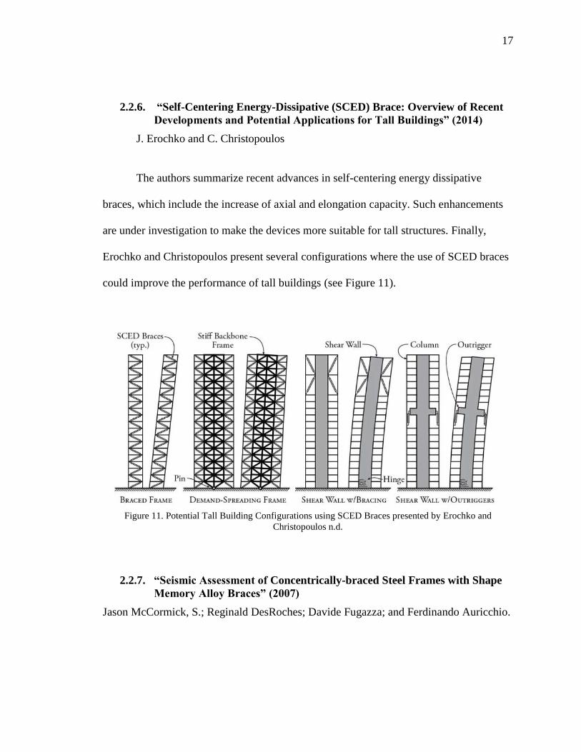
The authors summarize recent advances in self-centering energy dissipative
braces, which include the increase of axial and elongation capacity. Such enhancements
are under investigation to make the devices more suitable for tall structures. Finally,
Erochko and Christopoulos present several configurations where the use of SCED braces
could improve the performance of tall buildings (see Figure 11).
Figure 11. Potential Tall Building Configurations using SCED Braces presented by Erochko and
Christopoulos n.d.
2.2.7. “Seismic Assessment of Concentrically-braced Steel Frames with Shape
Memory Alloy Braces” (2007)
Jason McCormick, S.; Reginald DesRoches; Davide Fugazza; and Ferdinando Auricchio.

18
The high self-centering capability of Shape Memory Alloy Braces was exhibited by
comparing one three story and one six story conventional steel braced frame with
equivalent frames equipped with SMA braces. Maximum interstory drift and residual
roof displacement were compared with and without SMA braces. The SMA braces were
more effective in the shorter building, and similarly for the first floors of the taller
building. For the tall and higher floors, no significant favorable effects were observed
(McCormick et al. 2007).
2.2.8. “An innovative seismic bracing system based on a shape memory alloy
ring,” (2016).
Nan Gao, Jong-Su Jeon, Darel E Hodgson and Reginald DesRoches.
Figure 12. Right: Experimental setup: (a) loading test frame, (b) SMA ring and steel connections, (c)
turnbuckle and custom-made load cell, and (d) pad-eye connection and LVDT. Left: a Cross-braced system
based on an SMA ring (Gao et al. 2016)

19
The authors introduced a new bracing system using SMA rings and wires (see
Figure 12, right). Analyses were performed using an Abaqus finite element model to
simulate the SMA ring behavior. The experimental design used to calibrate the FE model
is also shown. The main difference between this study and its predecessors is the
adoption of a ring as the key structural component (see Figure 12, left), which Gao et al.
argued had a higher capacity (larger sections) and was easier to fabricate than other
competing SMA designs. This proposed bracing system showed less self-centering
capability compared with previous SMA-based braces, but exhibited larger energy
dissipation and lateral stiffness. Gao et al. acknowledged that the system did not perform
as expected, and urged that further studies on SMA sensitivity to temperature and loading
rate have to be conducted before drawing final conclusions about the capabilities of their
bracing system.
2.2.9. “Seismic resistant rocking coupled walls with innovative Resilient Slip
Friction (RSF) joints” (2017)
Ashkan Hashemi, Pouyan Zarnani, Reza Masoudnia, Pierre Quenneville.
Figure 13. Right: RSF joint: a) Cap plates and slotted center plates b) Belleville springs c) High strength
bolts d) Assembly of the joint. Left: Schematic load-deformation loop for the RSF joint.

20
This study examines the performance of Resilient Slip Friction (RSF) joints when
applied to coupling timber walls. The RSF joint, consisting of friction plates with grooves
and springs assembled into a compact device (Figure 13), was first introduced by Dr.
Zarnani (Provisional patent no.7083, 2015). The device provides the structural system
with extra damping and self-centering capabilities. The authors concluded that RDF
joints significantly help to dissipate energy through friction. The authors also noted the
potential for implementation in steel and reinforced concrete structures (Hashemi et al.
2017).
2.3. Earthquake Loss Assessment
A thorough understanding of strong ground motion effects on societal
functionality is a crucially important step toward hazard mitigation. For many years, the
structural engineering field was almost exclusively concerned with avoiding casualties
during seismic events. As the field became more proficient at this task, efforts have been
redirected towards measuring and quantifying socio-economic impacts. One example of
primary impacts is the repair cost to return a structure to a safe condition after incurring
damage. A secondary effect is the economic impact of business disruption caused by
inability to occupy a damaged structure. Would it be economically sound to retrofit
particular structures to mitigate potential losses? Would the cost of demolishing and
reconstructing the full structure offset any reparability effort? These are questions that
joint programs like HAZUS and P-58 developed by FEMA, the NIST Community
Resilience Program, and the Resilient Design Institute (RDI), have sought to address for

21
the last two decades. The following literature highlights the importance of rethinking
structural engineering regarding resiliency.
2.3.1. “Lessons from the February 22nd Christchurch Earthquake”
(2012)
Helen M. Goldsworthy
This work summarized the main structural flaws observed during the Christchurch
earthquake in 2011. There was a direct correlation between the age of the building and
the damage incurred. The older the structure, the greater the amount of damage that was
observed. This pattern found its explanation in the improved (especially at detailing) new
codes that have been implemented (Tremblay et al. 2008). Despite the fact that this work
was focused on reinforced concrete structures, it provides valuable insights that can be
extrapolated to other kinds of construction, such as soft story failures, damage
concentration, and non-structural damage. Goldsworthy concluded by urging the use of
displacement-based methods to quantify performance and recommending the adoption of
resilient solutions for high importance buildings (Goldsworthy 2012).
2.3.2. “Steel Building Damage from The Christchurch Earthquake Series of
2010 And 2011” (2012)
Charles Clifton, Michel Bruneau, Greg MacRae, Roberto Leon, and Alistair
Fussell
Selected steel structures were assessed to quantify damage suffered due to the
robust and successive ground motions. Special focus was placed on eccentrically braced
frames and moment resisting frames.

22
The preferred structural material for building construction in Christchurch has
historically been reinforced concrete due to easy access to aggregates in the area.
Therefore, by 2010 when the first strong earthquake happened, most relevant steel
structures had been built recently (Goldsworthy 2012). Overall, these steel structures
showed outstanding performance at the life-safety level because they met the most
current code standards.
Figure 14. Christchurch parking lot [Photos by M. Bruneau]; (a) inelastic deformations at top level EBF;
(b) Fractured link at lower level EBF. (Clifton et al. 2011)
Steel-frame connections generally performed as expected. Eccentrically-braced
frames also showed satisfactory response with limited exceptions where link fracture was
observed (see Figure 14b). On the other hand, concentrically-braced frames commonly
experienced brace fractures (see Figure 15).
The steel structures’ overall performance has encouraged Christchurch authorities
to implement more steel construction and to increase the research and development of
innovative self-centering devices to reduce downtime, building content losses, and non-
structural damage.
(a) (b)

23
Figure 15. Low‐rise CBF parking garage [Photos by M. Bruneau]. (a) Buckled brace; (b) Fractured non‐
ductile brace‐to‐column connection (Clifton et al. 2011).
2.3.3. “Estimation of Seismic Acceleration Demands in Building Components”
(2004)
Shahram Taghavi, Eduardo Miranda
Figure 16. Acceleration-sensitive nonstructural components (Taghavi, Shahram; Miranda 2004).
Generally, after a strong ground motion, nonstructural damage represents a
significant portion of the total cost of building repair. Thus, Taghavi and Miranda
(a) (b)
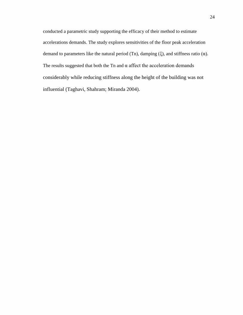
24
conducted a parametric study supporting the efficacy of their method to estimate
accelerations demands. The study explores sensitivities of the floor peak acceleration
demand to parameters like the natural period (Tn), damping (ξ), and stiffness ratio (α).
The results suggested that both the Tn and α affect the acceleration demands
considerably while reducing stiffness along the height of the building was not
influential (Taghavi, Shahram; Miranda 2004).
25
CHAPTER 3. OBJECTIVES AND SCOPE.
3.1. Objectives
To identify preferable characteristics for a hyperelastic fuse, the following research
objectives were selected.
Identify beneficial combinations of the hyperelastic component parameters (i.e.
stiffness, ductility, elastic buckling force), that provide superior or comparable
mechanical responses to those of conventional hysteretic systems. Performance
was evaluated based on peak mechanical force and displacements.
Perform earthquake loss assessment estimates to evaluate the competitiveness of
hyperelastic systems compared to hysteretic systems available in current practice,
such as Buckling Restrained Braces (BRBs). These evaluations were conducted
regarding earthquake mainshock repair cost.
3.2. Scope
The extent of this work is limited as follows:
Buildings with significant irregularities and thus torsional and higher mode effects
are not considered. Therefore, simplified SDOF models were reasonably
representative for the analyses.
The prototype buildings used in the study were assumed to be located in high
seismicity areas. Specifically, Los Angeles, CA was used as the referenced
location in this work.
Steel-braced, low-rise buildings, with a natural period (Tn) ranging from 0.1 to
0.4 seconds.

26
The multi-linear behavior of the hyperelastic system was characterized using three
stiffness categories: initial (K0), buckled (K2), and arresting (K3).
Comparable hyperelastic and hysteretic systems were assumed to have equal
initial stiffnesses (K0).
It is intended that all lateral loads have to be resisted by the braces exclusively.
Hence, all building connections are pinned (i.e. column-foundation, beam-
column, brace-column.)
Second order effects (P-Delta) were not explicitly addressed.

27
CHAPTER 4. METHODOLOGY
Over 1500 single degree of freedom (SDOF) analyses were carried out using
various combinations of constitutive parameters and nonlinear time history methods with
a suite of scaled ground motions. The analyses sought to identify beneficial combinations
of hyperelastic component parameters. The findings present hyperelastic system
performance in context relative to performance available from an alternative hysteretic
system. Hyperelastic models were parameterized with respect to a buckling force limit,
ductility to an arresting stiffening branch, and the ratio of arresting to initial stiffness.
Four low-rise, concentrically-braced, buildings were used as prototypes for the
comparisons. These structures were modeled as SDOFs by isolating the first mode
response.
Performance is quantified in terms of direct capital-related loss, defined as the
repair expenses as a percentage of total building replacement cost (total cost of structure,
nonstructural components, and contents). Moreover, sensitivities of loss measures to
hyperelastic characteristics were examined with respect to nonlinear dynamic ground
motion response using a representative suite of ground motions for Southern California.
4.1. Prototype Buildings
This study was conducting using structural characteristics representative of
single- and three-story, concentrically-braced frame (CBF) buildings that might be found
in metropolitan Los Angeles or sites with similar seismic demands.
Preliminary design for prototype buildings was performed to satisfy ASCE 7-10
seismic requirements for new commercial office buildings. Ordinary (OCBFs) and

28
Special (SCBFs) seismic detailing scenarios were selected as baseline hysteretic options
to explore design ductility influence on the relative performance of hysteretic and
hyperelastic systems. Hence, four prototype buildings were examined as shown in Table
1:
Table 1. Prototype buildings (CASES)
No. of
Stories
Seismic Detailing
Ordinary Special
1 CASE C CASE A
3 CASE D CASE B
A building plan and elevation were adapted from the 3-story LA building (see
Figure 17) reported by the SAC Joint Venture (FEMA 2000). Floor dimensions were 80 x
120 ft (24x36 m) for all buildings. Floor framing spans were 20 ft (6 m) in both
directions. The bold lines in Figure 17a represent the braced frame locations (A3-6, E3-6,
1A-D, and 7A-D). Story heights were 13 ft (4 m) for both 1-story and 3-story buildings
(see Figure 17b Figure 17c).

29
Figure 17. Prototype Buildings. (a) Plan view; (b) 3-Story Elevation view; (c) 1-Story Elevation view
4.2. Design of Prototype Buildings
Preliminary analyses were performed using SAP2000 (see Figure 18), in which all
floors were assumed to have a total dead load (self plus superimposed weight) of 100
lb/ft2 (488 kg/m2). The study considered a uniform live load of 80 lb/ft2 (390 kg/m2).
These loads approximately represent the concrete on steel deck flooring (~50 psf),
partitions (~25 psf), ceiling (~7psf), supporting steel floor framing (~18psf), office
personnel traffic (~50 psf), and furniture of commercial office buildings (~30 psf). All
columns and beams were assumed to be W-shapes A992 Grade 50 steel, and all braces
were assumed to be HSS with A500 Grade B steel. All load combinations related to the
1-STORY
3-STORY
(a)
(b)
(c)
N

30
dead, live, and earthquake load cases were considered for both analysis and design. All
elements’ boundary conditions were pinned (no moments).
Figure 18. 3D analysis models; SAP2000; (a) 3-Story; (b) 1-Story
4.2.1. Equivalent Lateral Force (ELF)
Figure 17 shows that the lateral force resisting system of the buildings is
symmetric and orthogonal, which permits uncoupling the braced frames’ contributions to
the LFRS. In this context, the buildings’ nature (short, symmetric, and orthogonal)
validates the applicability of the ELF procedure to design all prototype buildings
(ASCE/SEI 2010).
(a)
(b)

31
4.2.2. Response Modification Coefficient R.
The CBFs under consideration are either Ordinary or Special with respect to
seismic detailing. Therefore, the two base response modifications factors (R) used were
3.25 and 6, respectively, as shown in Table 2.
Table 2. Design Coefficients and Factors for Seismic Force-Resisting Systems of the ASCE/SEI 2010.
4.2.2.1. Design Category, Spectral Accelerations (SDS and SD1)
Based on the site conditions assumed (Site Class D, Los Angeles) and the risk
category of typical commercial office buildings (II), the USGS U.S. Seismic Design
Maps provided a design spectral acceleration in the short period range (SDS) of 1.36 g
and design spectral acceleration at 1 second (SD1) of 0.717 g. Accordingly, the prototype
buildings fall in the most severe design category, D, in accordance with Table 11.61 and
11.62 (ASCE/SEI 2010; USGS 2015).

32
4.2.2.2. Approximate Period
In order to compute the seismic load distribution by the ELF method, approximate
periods had to first be calculated. Approximate periods were calculated using ASCE
equation (12.8-7)
𝑇𝑎 = 𝐶𝑡 ∗ ℎ𝑛𝑥,
where, according to Table 3, 𝐶𝑡 = 0.02; 𝑥 = 0.75; and ℎ𝑛 = 𝑏𝑢𝑖𝑙𝑑𝑖𝑛𝑔 ℎ𝑒𝑖𝑔ℎ𝑡 [𝑓𝑡].
For instance, for the 3-story building 𝑇𝑎2 = 0.02 ∗ 390.75 = 0.312 𝑠𝑒𝑐; while for the 1-
Story building 𝑇𝑎1 = 0.137 sec.
Table 3. ASCE 7-10 Parameters to compute Approximate Period.
4.2.2.3. Vertical Distribution of Lateral Loads
Preliminary design base shear (V) was computed as follows. First, base shear
coefficients (Cs) were determined for each prototype structure:
𝐶𝑆 =𝑆𝐷𝑆 ∗ 𝐼𝑒
𝑅 ≤
𝑆D1 ∗ 𝐼𝑒
𝑅 ∗ 𝑇 𝑓𝑜𝑟 𝑇 ≤ 𝑇𝐿
Where:
𝑆𝐷1 = 0.717 𝑔

33
𝑆𝐷𝑆 = 1.360 𝑔
𝑇𝐿 = 8 𝑠𝑒𝑐𝑜𝑛𝑑𝑠
For the 3-story building (Tn ≈ 0.312 sec) with high ductility (R = 6):
𝐶𝑆 =1.36 ∗ 1
6≤
0.717 ∗ 1
6 ∗ 0.312
𝐶𝑆 = 0.22667 ≤ 0.3829
𝑪𝑺 = 𝟎.22667
Check if 𝐶𝑆 > 0.044 ∗ 𝑆𝐷𝑆 ∗ 𝐼𝑒 ≥ 0.01
𝐶𝑆 > 0.044 ∗ 1.360 ∗ 1 ≥ 0.01
𝐶𝑆 > 0.05984 ≥ 0.01
Because 𝑆𝐷1 = 0.717 ≥ 0.6 𝑔, it is required to check that 𝐶𝑆 ≥0.5∗𝑆1∗𝐼𝑒
𝑅
𝐶𝑆 ≥0.5 ∗ 0.717 ∗ 1
6
𝐶𝑆 ≥ 0.0598
Then the 𝑪𝑺 for the 3-story building with special seismic design (R=6) equals:
𝑪𝑺 = 𝟎.2267
Performing a similar analysis for the other three prototype building confirmed that all
cases were governed by the acceleration-controlled region of the elastic design spectrum.
The design 𝑪𝑺 values were as shown in Table 4:
Table 4. Seismic Response Coefficients (Cs) for all Prototype Buildings
3-story SCBF
(R = 6)
One story – SCBF
(R = 6)
Three story – OCBF
(R = 3.25)
One story – OCBF
(R = 3.25)
0.2267 0.2267 0.4185 0.4185

34
After inputting these Cs values into the corresponding SAP 2000 models, the base
shears were computed and subsequently distributed through the structures’ height as
equivalent lateral forces. The general equation for seismic base shear is found from the
product of the seismic response coefficient (Cs) and the seismic weight (W, i.e., the
assumed dead load of each structure):
𝑉 = 𝐶𝑆 ∗ 𝑊,
While the vertical distribution of lateral forces computed by the program used the following
equations:
𝐹𝑖 = 𝐶𝑣𝑖 ∗ 𝑉,
where:
𝐶𝑣𝑖 = 𝑊𝑖 ∗ ℎ𝑖
𝑘
∑ 𝑊𝑗 ∗ ℎ𝑗𝑘𝑁
𝑗=1
𝑘 = 1 𝑓𝑜𝑟 𝑇 ≤ 0.5𝑠;
𝑘 = 2 𝑓𝑜𝑟 𝑇 => 2.5𝑠;
𝑘 = 𝑙𝑖𝑛𝑒𝑎𝑟 𝑖𝑛𝑡𝑒𝑟𝑝𝑜𝑙𝑎𝑡𝑖𝑜𝑛 𝑏𝑒𝑡𝑤𝑒𝑒𝑛 1 𝑎𝑛𝑑 2 𝑓𝑜𝑟 𝑇 = 0.5 − 2.0𝑠
Furthermore, after designing the buildings using SAP2000 (beam, columns, and braces)
to satisfy the AISC requirements and obtaining the final natural periods, they were
checked to be less than 𝑇𝑆𝐴𝑃2000 ≤ 𝐶𝑢 ∗ 𝑇𝑎.
𝑇𝑆𝐴𝑃2000 ≤ 𝐶𝑢 ∗ 𝑇𝑎 = 1.4 ∗ 0.312 = 0.44 𝑠𝑒𝑐
Where; 𝐶𝑢 = 1.4 from Table 5.
𝑇𝑆𝐴𝑃2000 = 0.4 ≤ 0.44 sec OK!
.

35
Table 5. ASCE 7-10 Upper Limit on Calculated Period (from Table 12.8-1).
The final calculated periods are listed in Table 6.
Table 6. Natural Periods of Prototype Buildings
Parameters
under
Evaluation
Period Tn [s]
3-story SCBF
(R = 6) 1 story – SCBF
(R = 6) 3 stories – OCBF
(R = 3.25) 1 story – OCBF
(R = 3.25)
𝐶𝑢 ∗ 𝑇𝑎 0.44 0.20 0.44 0.19
X direction 0.40 0.21 0.32 0.18
Y direction 0.40 0.20 0.29 0.17
Tn SDOF 0.40 0.20 0.31 0.17
4.3. Prototype Buildings Simplification to Single Degree of
Freedom (SDOF) Systems
Once all columns, beams, and braces were proportioned to meet preliminary
strength design requirements, the 3-story buildings were converted into equivalent SDOF
systems by using the modal participation factor to isolate the first mode response. The
analysis of MDOF systems (3-story cases) based on a single mode is valid because more
than 90% of the seismic mass participated effectively in the first mode. Additionally, the
symmetry of the buildings suppresses torsional effects. The equivalent SDOF systems
consist of an effective modal mass (Msdof), and effective modal height (hsdof) (damping:

36
5% of the critical). This simplification is illustrated in Figure 19, an illustration from the
book “Dynamics of Structures” by Anil K. Chopra, 2012.
Figure 19. Chopra illustration for effective modal masses and heights (Chopra 2012).
The floor seismic mass of the buildings (labeled ‘m’ in Figure 19) was computed by
factoring the floor area times the distributed dead load, 𝑚 = 𝐴𝑓𝑙𝑜𝑜𝑟 ∗ 𝐷𝐿. With the
stiffness and mass matrices assembled, natural frequencies and mode shapes were
computed through the eigenvalue formulation. After that, modal participation factors and
SDOFs masses (mSDOF) were calculated. Representative modal stiffnesses were calculated
using natural periods and modal masses from SAP2000.
A summary of the SDOF characteristics systems considered in this study is presented
below (Table 7).

37
Table 7. Summary table equivalent SDOF systems
Calculated Parameters
Equations
3-story-
High
Ductility
(R = 6)
1 story –
High
Ductility
(R = 6)
3 stories – Low
Ductility
(R = 3.25)
1 story – Low
Ductility
(R = 3.25)
mSDOF [kg] 𝛤1
∗ ∑ 𝑚𝑗𝛷1𝑗
𝑗
891781 297260 891781 297260
ωn_SDOF Eigen Value 15.7 31.4 20.2 36.9
Tn_SDOF [sec] 2𝜋
𝜔𝑛 0.4 0.2 0.31 0.17
K0_SDOF [N/m] 𝜔𝑛2 ∗ 𝑚𝑆𝐷𝑂𝐹 220038142 293383860.4 366348623.6 406067627
ξ [% of CR] 𝐶
2 ∗ 𝑚𝑆𝐷𝑂𝐹 ∗ 𝜔𝑛 5 5 5 5
4.4. Ground Motions
A suite of 16 records was selected to match some of those considered in the
“Seismic response of self-centring hysteretic SDOF systems” conducted by professors
Chirstopolous et al. in 2001. The ground motions were scaled to a target 5% damped
elastic design spectrum for soil type D conditions in Los Angeles area. These historically
strong ground motions were used to evaluate the seismic performance of all prototype
buildings. The scaled suite is intended to represent earthquakes with a probability of
exceedance of 10% in a 50-year hazard level, approximated as 2/3 of the MCE
(maximum considered earthquake), consistent with ASCE 7-10. (FEMA 2000; Tremblay
et al. 2008).
The motions were obtained from the NGA-West2 on-line Ground-Motion
Database created by experts at the Pacific Earthquake Engineering Research Center
(PEER) (Ancheta et al. 2013). Table 8 and Table 9 present the main characteristics of the
ground motions used in this study.
38
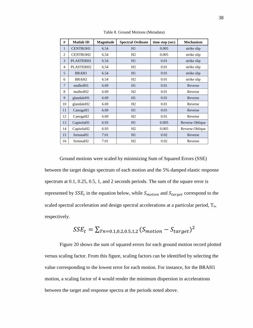
Table 8. Ground Motions (Metadata)
# Matlab ID Magnitude Spectral Ordinate time step (sec) Mechanism
1 CENTROH1 6.54 H1 0.005 strike slip
2 CENTROH2 6.54 H2 0.005 strike slip
3 PLASTERH1 6.54 H1 0.01 strike slip
4 PLASTERH2 6.54 H2 0.01 strike slip
5 BRAH1 6.54 H1 0.01 strike slip
6 BRAH2 6.54 H2 0.01 strike slip
7 mulholH1 6.69 H1 0.01 Reverse
8 mulholH2 6.69 H2 0.01 Reverse
9 glandaleH1 6.69 H1 0.01 Reverse
10 glandaleH2 6.69 H2 0.01 Reverse
11 CanogaH1 6.69 H1 0.01 Reverse
12 CanogaH2 6.69 H2 0.01 Reverse
13 CapitolaH1 6.93 H1 0.005 Reverse Oblique
14 CapitolaH2 6.93 H2 0.005 Reverse Oblique
15 fortunaH1 7.01 H1 0.02 Reverse
16 fortunaH2 7.01 H2 0.02 Reverse
Ground motions were scaled by minimizing Sum of Squared Errors (SSE)
between the target design spectrum of each motion and the 5% damped elastic response
spectrum at 0.1, 0.25, 0.5, 1, and 2 seconds periods. The sum of the square error is
represented by 𝑆𝑆𝐸𝑡 in the equation below, while 𝑆𝑚𝑜𝑡𝑖𝑜𝑛 and 𝑆𝑡𝑎𝑟𝑔𝑒𝑡 correspond to the
scaled spectral acceleration and design spectral accelerations at a particular period, Tn,
respectively.
𝑆𝑆𝐸𝑡 = ∑ (𝑆𝑚𝑜𝑡𝑖𝑜𝑛 − 𝑆𝑡𝑎𝑟𝑔𝑒𝑡)2𝑇𝑛=0.1,0.2,0.5,1,2
Figure 20 shows the sum of squared errors for each ground motion record plotted
versus scaling factor. From this figure, scaling factors can be identified by selecting the
value corresponding to the lowest error for each motion. For instance, for the BRAH1
motion, a scaling factor of 4 would render the minimum dispersion in accelerations
between the target and response spectra at the periods noted above.

39
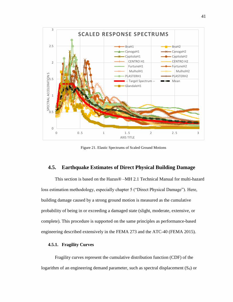
Scaling factors are reported in the last column of Table 9 for each ground motion.
Additionally, the response spectrums of the scaled motions are plotted against the target
design spectrum for visual comparison in Figure 21.
Figure 20. Scaling Factors
Each recorded direction was considered separately in analyses (as obtained from
the PEER strong motion database). Moreover, the end of all of the records was filled with
20 zeros to measure residual displacements accurately; this created a free vibration phase
until the damping abates inertial effects.

40
Table 9. Ground Motions’ Scaling Factors
# Matlab ID Record Earthquake
Name Year Station Name
Vs30
(m/sec)
Scale
Factor
1 CENTROH1 RSN721-
ICC000
Superstition
Hills-02 1987
El Centro Imp. Co.
Cent 192.05 2
2 CENTROH2 RSN721-
ICC090
Superstition
Hills-02 1987
El Centro Imp. Co.
Cent 192.05 2.1
3 PLASTERH1 RSN724-
PLS045
Superstition
Hills-02 1987 Plaster City 316.64 5
4 PLASTERH2 RSN724-
PLS135
"Superstition
Hills-02" 1987 Plaster City 316.64 2.7
5 BRAH1 RSN719 -
BRA225
Superstition
Hills-02 1987 Brawley Airport 208.71 4
6 BRAH2 RSN719-
BRA315
Superstition
Hills-02 1987 Brawley Airport 208.71 3.4
7 mulholH1 RSN953-
MUL009 Northridge-01 1994
Beverly Hills -
14145 Mulhol 355.81 1
8 mulholH2 RSN953-
MUL279 Northridge-01 1994
Beverly Hills -
14145 Mulhol 355.81 0.7
9 glandaleH1 RSN974-
GLP177 Northridge-01 1994
Glendale - Las
Palmas 371.07 1.3
10 glandaleH2 RSN974-
GLP267 Northridge-01 1994
Glendale - Las
Palmas 371.07 2.5
11 CanogaH1 RSN959-
CNP106 Northridge-01 1994
Canoga Park -
Topanga Can 267.49 1.5
12 CanogaH2 RSN959-
CNP196 Northridge-01 1994
Canoga Park -
Topanga Can 267.49 1.4
13 CapitolaH1 RSN752-
CAP000 Loma Prieta 1989 Capitola 288.62 1.1
14 CapitolaH2 RSN752-
CAP090 Loma Prieta 1989 Capitola 288.62 1.5
15 fortunaH1 RSN827-
FOR000
Cape
Mendocino 1992
Fortuna - Fortuna
Blvd 457.06 4.4
16 fortunaH2 RSN827-
FOR090
Cape
Mendocino 1992
Fortuna - Fortuna
Blvd 457.06 4.2
41
Figure 21. Elastic Spectrums of Scaled Ground Motions
4.5. Earthquake Estimates of Direct Physical Building Damage
This section is based on the Hazus® –MH 2.1 Technical Manual for multi-hazard
loss estimation methodology, especially chapter 5 (“Direct Physical Damage”). Here,
building damage caused by a strong ground motion is measured as the cumulative
probability of being in or exceeding a damaged state (slight, moderate, extensive, or
complete). This procedure is supported on the same principles as performance-based
engineering described extensively in the FEMA 273 and the ATC-40 (FEMA 2015).
4.5.1. Fragility Curves
Fragility curves represent the cumulative distribution function (CDF) of the
logarithm of an engineering demand parameter, such as spectral displacement (Sd) or
0
0.5
1
1.5
2
2.5
3
0 0 . 5 1 1 . 5 2 2 . 5 3
SPEC
TRA
L A
CC
ELER
ATI
ON
S
AXIS TITLE
SCALED RESPONSE SPECTRUMS
BraH1 BraH2
CanogaH1 CanogaH2
CapitolaH1 CapitolaH2
CENTRO H1 CENTRO H2
FurtuneH1 FurtuneH2
MulholH1 MulholH2
PLASTERH1 PLASTERH2
-- Target Spectrum -- Mean
GlandaleH1

42
spectral acceleration (Sa). In other words, these curves (see Figure 22) represent the
vulnerability in terms of probability of a building being in or exceeding a particular
damage state. For instance, in Figure 22, a building with 5 inches of peak displacement
would have approximately 100%, 50%, 5%, and 0% probabilities of exceeding the slight,
moderate, extensive, or complete damage stages, respectively.
Regarding the engineering demand parameters, the direct economic loss module
of HAZUS-MH uses displacement to assess damage to structural and drift-sensitive
nonstructural components. Whereas, acceleration is used to calculate acceleration-
sensitive nonstructural damage and contents losses.
Figure 22 HAZUS-MH Example of Fragility Curves for Slight, Moderate, Extensive and Complete
Damage

43
The probability of being in or exceeding a damage state is given by the equation below,
which was taken from HAZUS-MH technical manual, page 1-40.
𝑃[𝑑𝑠|𝑆𝑑] = 𝛷 [1
𝛽𝑑𝑠ln (
𝑆𝑑
𝑆𝑑,𝑑𝑠)]
where:
𝑺𝒅,𝒅𝒔: the median value of spectral displacement at which the building reaches the
threshold of the damage state, ds.
𝜷𝒅𝒔: the standard deviation of the natural logarithm of spectral displacement of
damage state, ds.
𝜱: the standard normal cumulative distribution function.
All prototype building structures were labeled as S2L, which stands for the low-
rise steel-braced frame (see Table 10). Moreover, because buildings were assumed to be
commercial, the corresponding occupancy classification was COM4, which stands for
offices offering technical or professional services. Structure classifications determine
damage state thresholds, and occupancy classifications determine relative proportions of
building value associated with structural and nonstructural components and contents.
Table 10. Building Model Classification (from Table 3.1 HAZUS-MH).
44
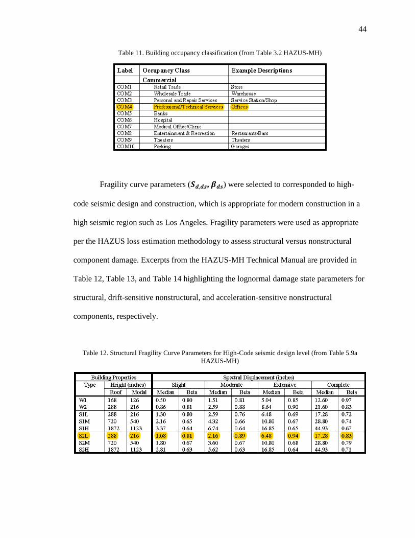
Table 11. Building occupancy classification (from Table 3.2 HAZUS-MH)
Fragility curve parameters (𝑺𝒅,𝒅𝒔, 𝜷𝒅𝒔) were selected to corresponded to high-
code seismic design and construction, which is appropriate for modern construction in a
high seismic region such as Los Angeles. Fragility parameters were used as appropriate
per the HAZUS loss estimation methodology to assess structural versus nonstructural
component damage. Excerpts from the HAZUS-MH Technical Manual are provided in
Table 12, Table 13, and Table 14 highlighting the lognormal damage state parameters for
structural, drift-sensitive nonstructural, and acceleration-sensitive nonstructural
components, respectively.
Table 12. Structural Fragility Curve Parameters for High-Code seismic design level (from Table 5.9a
HAZUS-MH)
45
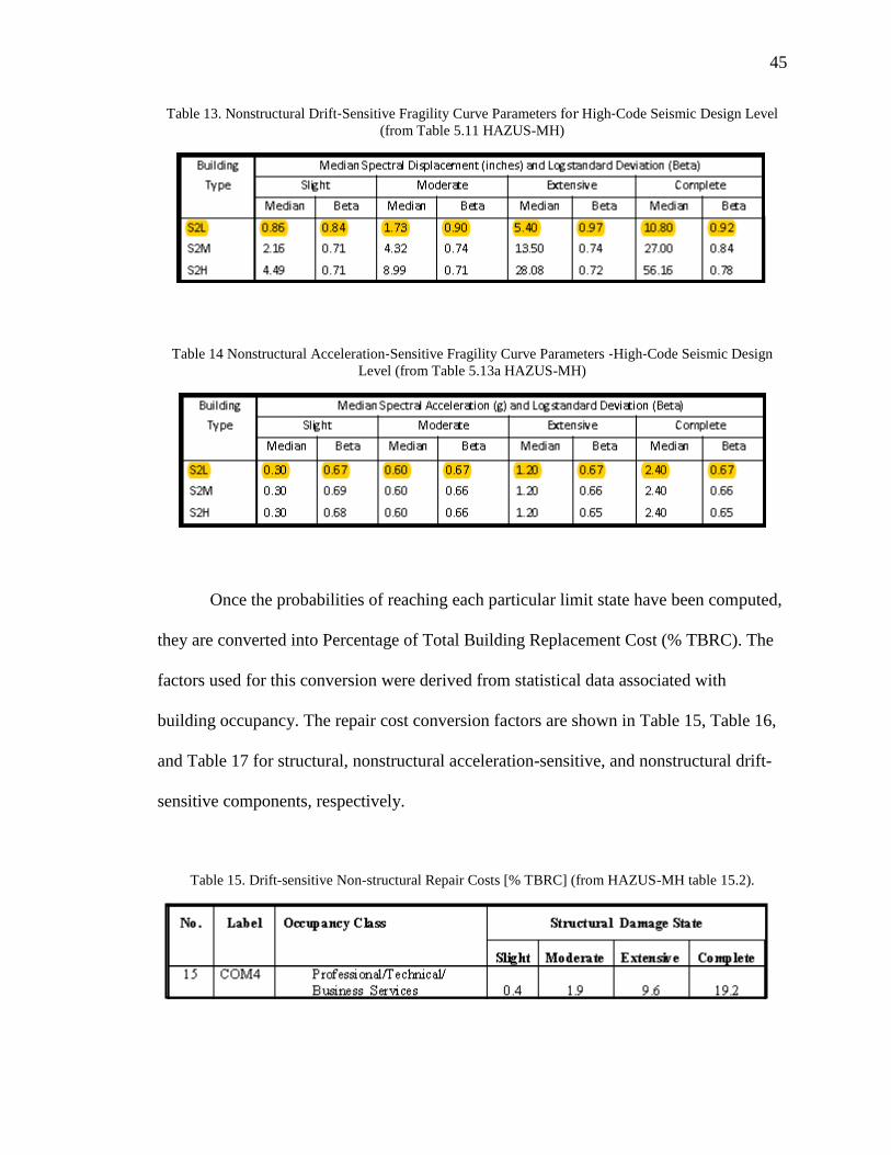
Table 13. Nonstructural Drift‐Sensitive Fragility Curve Parameters for High‐Code Seismic Design Level
(from Table 5.11 HAZUS-MH)
Table 14 Nonstructural Acceleration‐Sensitive Fragility Curve Parameters ‐High‐Code Seismic Design
Level (from Table 5.13a HAZUS-MH)
Once the probabilities of reaching each particular limit state have been computed,
they are converted into Percentage of Total Building Replacement Cost (% TBRC). The
factors used for this conversion were derived from statistical data associated with
building occupancy. The repair cost conversion factors are shown in Table 15, Table 16,
and Table 17 for structural, nonstructural acceleration-sensitive, and nonstructural drift-
sensitive components, respectively.
Table 15. Drift-sensitive Non-structural Repair Costs [% TBRC] (from HAZUS-MH table 15.2).

46
Table 16. Acceleration-sensitive Non-structural Repair Cost Ratios [% TBRC] (from HAZUS-MH table
15.3).
Table 17. Structural Repair Cost Ratios [% TBRC] (from HAZUS-MH table 15.4).
On the other hand, strong ground motions can also induce damage to building
contents. Therefore, contents losses were taken into account for all analyses. Contents
include any equipment or furniture that is not integrally attached to the structure, such as
computers, screens, and projectors. Contents damage is usually associated with building
accelerations. Therefore, quantifying contents damage can be related to the nonstructural
acceleration-sensitive estimations. For this task, FEMA developed Table 18 to estimate
contents losses based on the state of nonstructural acceleration-sensitive damage.
Table 18. Contents Damage Ratios (in % of contents replacement cost) (from Table 5.15 HAZUS-MH)

47
An example to clarify this process is presented in Table 19. Here, loss estimates
for structural (STR), nonstructural drift-sensitive (NSDS), nonstructural acceleration-
sensitive (NSAS), and contents of an example structure are calculated using the HAZUS-
MH methodology. For this task, 𝑃[𝑑𝑠|𝑆𝑑] equation (page 42) was applied three times.
The inputs were the spectral (peak) displacement (Sd) for STR and NSDS loss projections,
and the spectral (peak) acceleration (Sa) for NSAS loss assessments. For all cases the
values of 𝑺𝒅,𝒅𝒔 (Sd_bar) and 𝜷𝒅𝒔(beta) are found in Table 12, Table 13, and Table 14. Once
the probability of being in or exceeding a limit state is determined (PE), the probability of
not reaching such a state of damage (PDS) can be directly computed. For instance, in
Table 19 it was shown that the PE for at least slight structural damage was 33% and
therefore the PDS for “no damage” would equal 66% (66% chance of having zero
structural damage in the structure). Similarly, the PE for moderate structural damage was
23.5%, which rendered a 10% PDS for the slight structural damage state, 10% chance of
having slight structural damage (33% at least Slight (including Moderate and greater) -
23.5% at least Moderate = 10% probability of Slight damage).
An identical process was followed for all STR, NSDS, and NSAS damage states
[None, Slight (S), Moderate (M), and Complete (C)]. Then all PDS values were multiplied
by the appropriate repair cost ratios (from Table 15, Table 16, and Table 17) to obtain
building repair costs as a percentage of the total building replacement cost. For the
contents damage assessment, the process is slightly shorter because the previously
calculated PDS values for of the nonstructural acceleration-sensitive components (NSAS)
are multiplied by the content damage ratios (Table 18) to produce the content repair
costs.

48
Once all the repair costs have been estimated for individual components and
damage states, the costs are summed to produce a total estimated repair cost (loss). For
this particular example (Table 19), the HAZUS methodology indicated that repair costs
for a commercial office building, which sustained a 0.49 in (12.5 mm) peak displacement
and 0.4185 g (4.1 m/s2) peak acceleration, would cost, on average, approximately 24.9%
of the total building replacement cost. Here, it can also be seen that most of the damage
came from nonstructural acceleration-sensitive and building contents losses.
Analogous direct economic capital-related loss estimates were conducted for
hundreds of structural hyperelastic structural configurations as well as their hysteretic
counterparts. The structural damage was considered negligible for all hyperelastic models
because of the intended lack of inelastic deformations in the lateral load resisting system.

49
Table 19. Example of Direct Physical Building Damage Computation using HAZUS-MH, inputs’ units
Sd=[in] and Sa=[g]
24.9
Tota
l Sum
Los
s
[% T
BRC]
COM
4Lo
ssSu
m L
oss
00.
000
10.
178
50.
802
252.
964
506.
440
ΣCO
NT
10.4
CONTENTS
10.3
8
Sd
bar
beta
*Sd
/ Sd
bar
*lo
g (*
)lo
g (*
) / b
eta
PECO
M4
Loss
Sum
Los
s
Sd0.
49N
one
0.66
00.
00
Slig
ht0.
491.
080.
810.
454
-0.3
43-0
.424
0.33
6S
0.10
0.4
0.04
Mod
erat
e 0.
492.
160.
890.
227
-0.6
44-0
.724
0.23
5M
0.12
1.9
0.22
Exte
nsiv
e0.
496.
480.
940.
076
-1.1
21-1
.193
0.11
6E
0.09
9.6
0.82
Com
plet
e0.
4917
.28
0.83
0.02
8-1
.547
-1.8
640.
031
C0.
0319
.20.
60
Sd0.
49N
one
0.61
00.
00
Slig
ht0.
490.
860.
840.
570
-0.2
44-0
.291
0.38
6S
0.11
0.7
0.08
Mod
erat
e 0.
491.
730.
90.
283
-0.5
48-0
.609
0.27
1M
0.13
3.3
0.43
Exte
nsiv
e0.
495.
40.
970.
091
-1.0
42-1
.074
0.14
1E
0.07
16.4
1.13
Com
plet
e0.
4910
.80.
920.
045
-1.3
43-1
.460
0.07
2C
0.07
32.9
2.37
Sa0.
4185
Non
e0.
410
0.00
Slig
ht0.
4185
0.3
0.67
1.39
50.
145
0.21
60.
585
S0.
180.
90.
16
Mod
erat
e 0.
4185
0.6
0.67
0.69
8-0
.156
-0.2
340.
408
M0.
164.
80.
77
Exte
nsiv
e0.
4185
1.2
0.67
0.34
9-0
.457
-0.6
830.
247
E0.
1214
.41.
71
Com
plet
e0.
4185
2.4
0.67
0.17
4-0
.759
-1.1
320.
129
C0.
1347
.96.
17
14.5
ΣSTR
+NS-
DS+
NS-
AS
STR
NS
DS
NS
AS
P D
S
1.68
4.02
8.81
CO
NT
EN
T L
OS
S
ST
RU
CT
UR
AL
AN
D
NO
NS
TR
UC
TU
RA
L L
OS
S

50
4.6. Parametrization
The performance of two structural models is evaluated in this work: a bilinear
elastoplastic (fully hysteretic without degradation) and a trilinear hyperelastic model. The
hyperelastic model represents a concentrically-braced frame equipped with innovative
hyperelastic fuses. The idealized force-displacement relationships of both systems are
shown in Figure 23. The main parameters describing the systems are:
Figure 23. (a) hysteretic system behavior; (b) hyperelastic system.
Hyperelastic
fe: Buckling force
k0: Initial stiffness
k2: Buckling stiffness
k3: Arresting stiffness
Δg: Gap closure displacement
Δe: Buckling displacement
Hysteretic
fy: Yielding force
kh0: Elastic stiffness and a
kh2: Plastic stiffness.
Δy: Yielding displacement
(a) (b)

51
The initial stiffness was assumed equal (kh0=K0) for both systems, hyperelastic
and hysteretic, through the entire study, and the yielding (kh2) and first post-buckling (K2)
stiffness were assumed zero for simplicity, disregarding potential strain hardening in the
hysteretic system or post-buckling strength in the hyperelastic system. Three independent
response parameters were selected for parameterization in the hyperelastic model: the
ratio of initial to buckling stiffness (α1), the ratio of initial stiffness to arresting stiffness
(α2), and ductility to the arresting stiffness (μ). Additionally, the hyperelastic buckling
force was taken as a fraction of the hysteretic yielding force (fy), then the force ratio
(fy/fe) became the fourth parameter evaluated.
μ =∆g
∆y; α1 =
𝑘2
𝑘0= 0; α2 =
𝑘3
𝑘0
4.6.1. Sensitivity Analysis.
In this part of the study, the primary goal was to identify how induvial
hyperelastic parameters affect the structural response (peak displacements and
mechanical force). First, using a single ground motion response, peak response trends
were identified. These trends were confirmed by running all ground motions. If such a
trend was valid for more than nine of the sixteen motions, this trend was studied in more
detail.
An example of this procedure is presented in Figure 24, where the influence of the
arresting stiffness (𝑘3 = α2 ∗ 𝑘0) in the final response was investigated. For this purpose,
the arresting stiffness ratio (α2) was varied from 0 (flat) up to 0.25 (K3 equals 25% of the
initial stiffness), while the ductility equals 1.5 and a buckling force is equivalent to half

52
the yielding force (fy/fe=2) of the reference hysteretic model (see Figure 24a). The
response pattern here suggested that increasing the arresting stiffness yields a linear
decrease in displacement and a linear increase in maximum force. In order to see if this
trend remained while changing the ductility, maximum response trend lines (MRTLs)
were created. One of these lines is shown in Figure 24b. This line was created by joining
the maximum displacement and force (Δmax, fmax) of every hyperelastic system in Figure
24a (steps 1 and 2). Once the line was generated, the MRTL was mirrored to the opposite
region (step 3) to compare maximum displacements against the hysteretic system at both
zones (blue lines in Figure 24c). Finally, Figure 24c shows several MRTLs plotted for
ductilities varying from 1.5 to 10 in 0.5 increments. Base on this figure, it was
demonstrated that the linear trend remained independent of the ductility used. Similar
sensitivity analyses were conducted for all three parameters evaluated (α2, μ, fy/fe ratio).
Once a trend was identified, the validity of the trend was verified. A trend was
considered valid if it was observed with at least nine of the sixteen considered ground
motion records.
In summary, this study identified the parameters governing the seismic behavior
of concentrically-braced frames equipped with hyperelastic structural fuses. Additionally,
it was analytically verified that it is possible to calibrate hyperelastic fuses to achieve
better or comparable performances (regarding peak mechanical force and displacements)
to that of comparable hysteretic systems.

53
Figure 24. Trend identification example by using maximum response trend lines (MRTLs)
(a) (b)
1 2
3
(c)

54
CHAPTER 5. RESULTS
5.1. Overview
The body of this chapter is divided between bilinear and trilinear hyperelastic system
evaluations. Within these two sections, the results for each prototype building are
discussed one by one (case D through case A). Comparative results for bilinear
hyperelastic systems are shown starting on page 55, and the trilinear system results are
discussed starting on page 63. Comprehensive summaries of observations are shown for
the main findings of the bilinear system evaluations as a whole and individually for each
trilinear system.
μ =∆g
∆y; α1 =
𝑘2
𝑘0= 0; α2 =
𝑘3
𝑘0
Figure 25. Idealized Force- Displacement curve. Hysteretic and Hyperelastic
K2≈0
∆e ∆g ∆emax
fe
femax
Deflections
Bra
ce f
orc
e
K0
K3
1
2 3
4
5
7
4
6
Kh0
Kh2≈0
Kh0
fy
∆hmax∆y
HYSTERETIC
SYSTEMHYPERELASTIC
SYSTEM
II III
I
IV

55
5.2. Evaluation of Bilinear Hyperelastic Models
This section explores the possibility of obtaining competitive self-centering features
from bilinear hyperelastic systems by trading off reductions in brace force and, ideally,
acceleration demands, in exchange for higher average peak displacements. Such bilinear
behavior is achieved by using a fuse with enough gap space so that the arresting stiffness
(K3) is never reached.
The main question to address is how much additional displacement will occur for a
bilinear hyperelastic system relative to a full hysteretic system? Figure 26 illustrates this
comparison, where a hysteretic reference system is plotted against possible bilinear
hyperelastic models. Although the hyperelastic (K0) and hysteretic (Kh0) initial stiffnesses
are portrayed as having different values (different elastic stiffness slopes), the numerical
values were equivalent (Kh0 = K0) for each of the four considered Cases (A through D).

56
Figure 26. Force-Displacement curve for bilinear hyperelastic systems.
5.2.1. Bilinear, 3-Story Building, Low-Ductility (CASE D)
As described in the Methodology chapter, case D refers to a building with a
natural period (Tn) of 0.31s. This period approximates a three story concentrically-braced
frame (CBF) building, such as the structure shown in figure 2. According to ASCE/SEI
2010, a response modification factor (R) of 3.25 can be used for seismic design when the
frame is proportioned and detailed in accordance with Ordinary CBF requirements.
Analysis results are presented in Table 20 and Figure 27, showing that the peak
displacement increased from 44% when fy/fe=1 to 1039% when the buckling force level
of the hyperelastic system was reduced to a third of the corresponding hysterestic system
yield strength, fy/fe=3. The viability of increasing the fy/fe ratio was explored further
while computing loss assessment estimates, results of which are presented in Figure 31.
Δe Δemax
fe
Deflections
Bra
ce f
orc
e
K0
fy
ΔhmaxΔy
K0
fy/fe ≈ 2
K0
Kh0
K0
K0
K0
K0
fy/fe
fy/fe
fy/fe
fy/fe≈1.5
fy/fe
fy/fe>3
Kh0 = K0
DUCTh= Δhmax / Δy
DUCTe= Δemax / Δe
=
=
=
=

57
Table 20. CASE D. Peak Ductility comparisons between Hysteretic and Bilinear Hyperelastic systems
(different fy/fe ratios.)
CASE D- Ductility
3-Story, Ordinary Seismic Design 3 Stories R=3.25 Tn=0.31
Ground
Motions
Duct_Hysteretic Duct_Hyperelastic -- (fy/fe)
0 1 1.1 1.2 1.5 2 3
CENTRO H1 4 7.43 9 10 22 44 51
CENTRO H2 4.16 5 8 8 13 23 78
PLASTERH1 6.8 9 9 13 16 28 33
PLASTERH2 5.4 5.7 8 8 8 18 39
BraH1 3.6 3.15 4 5 11 18 28
BraH2 2.3 1.55 3 3 6 7 13
MulholH1 2.93 2.67 7 9 59 85 127
MulholH2 2 5.5 8 9 11 16 47
GlandaleH2 1.4 1.79 2 3 3 7 8
GlandaleH1 1.45 2.5 3 4 5 6 8
CanogaH2 5.6 11.24 14 15 19 31 45
CanogaH1 5.3 6.64 8 8 15 26 41
CapitolaH2 6.8 9.1 14 15 17 18 28
CapitolaH1 4.6 4.8 5 5 17 23 42
FurtuneH2 4 8.64 9 13 20 26 69
FurtuneH1 6.8 12 8 15 18 23 108
Average 4.2 6.0 7.4 8.9 16.3 24.9 47.8
Max 6.8 12 14 15 59 85 127
Figure 27. CASE D. Ductility required for a Bilinear Hysteretic system, different fy/fe ratios.
0
20
40
60
80
100
120
140
0 0.5 1 1.5 2 2.5 3
DU
CTI
LITY
(SD
/dY
)
Fy/Fe [0 = Hysteretic]
CENTRO H1 CENTRO H2PLASTERH1 PLASTERH2BraH1 BraH2MulholH1 MulholH2GlandaleH2 GlandaleH1CanogaH2 CanogaH1CapitolaH2 CapitolaH1FurtuneH2 FurtuneH1Avarege

58
5.2.2. Bilinear, 1-story Building, Low-Ductility (CASE C)
As described in the methods chapter, case C refers to a building with a natural period
of 0.17 seconds. As with case D discussed previously, the R factor equals 3.25.
Table 21 and Figure 28 show the results for this particular building. Here, the increase
in displacement demands was more pronounced with a shorter period (higher elastic
stiffness). When fy equals fe, the average ductility for the hyperelastic system was 12
(116% increase over the hysteretic) while for fe=fy/3 the average ductility reached 94
(1593% increase over the hysteretic). Hence, the viability of increasing fy/fe was further
explored through HAZUS-MH. Those results are presented in Figure 31.
Table 21. CASE C. Peak Ductility comparisons between Hysteretic and Bilinear Hyperelastic systems
(different fy/fe ratios.)
CASE C- Ductility
1-Story, Ordinary Seismic Design 1 Stories R=3.25 Tn=0.17
Ground Motions Duct_Hysteretic Duct_Hyperelastic -- (fy/fe)
0 1 1.1 1.2 1.5 2 3
CENTRO H1 7.13 22.2 25 31 45 87 164
CENTRO H2 9.56 10.33 14 17 21 46 126
PLASTERH1 8.12 22.4 21 26 35 46 93
PLASTERH2 9.5 22.95 25 28 26 36 66
BraH1 4 6.76 7 8 19 26 71
BraH2 3.6 2.4 2 3 3 20 30
MulholH1 3.58 4.3 7 9 59 85 127
MulholH2 2.13 5.74 7 21 27 42 81
GlandaleH2 3 7.4 7 9 10 18 26
GlandaleH1 2.65 7.6 8 8 10 15 20
CanogaH2 6.5 26 28 32 51 65 96
CanogaH1 7.1 11.68 13 13 25 46 109
CapitolaH2 9.8 15.77 10 42 42 48 72
CapitolaH1 5.79 13.6 14 14 17 46 73
FurtuneH2 2.72 6.2 13 8 32 57 163
FurtuneH1 3.67 7 35 34 55 56 187
Average 5.6 12.0 14.8 18.9 29.8 46.2 94.0
Max 9.8 26 35 42 59 87 187

59
Figure 28. CASE C. Ductility required for a Bilinear Hysteretic system, different fy/fe ratios.
5.2.3. Bilinear, 3-story Building, High Ductility (CASE B)
As described in the methods chapter, case B refers to a 3-story building with a natural
period of 0.4 seconds. Case B represents a building designed for high seismic demands.
Therefore, the response modification factor (R) equals 6, corresponding to a structure
meeting requirements for Special CBFs (ASCE/SEI 2010). Table 22 and Figure 29 show
the results for this particular building. When the same force capacity is used for
hyperelastic and hysteretic systems (fy/fe=1), the average peak ductility required increases
60%, a ductility of 8.5 in the hysteretic versus a 13.6 of the hyperelastic. If the buckling
force in the hyperelastic (fe) is set to one-third of the hysteretic system yield strength (fy/fe
=3), the average ductility demand is 671% greater than that of the hysteretic system. The
economic viability of increasing the fy/fe was further explored through HAZUS-MH. The
results are presented in Figure 31.
0
50
100
150
200
0 0.5 1 1.5 2 2.5 3
DU
CTI
LITY
FY/FE [0 = HYSTERETIC]
CENTRO H1 CENTRO H2
PLASTERH1 PLASTERH2BraH1 BraH2MulholH1 MulholH2GlandaleH2 GlandaleH1CanogaH2 CanogaH1CapitolaH2 CapitolaH1FurtuneH2 FurtuneH1

60
Table 22. CASE B. Peak Ductility comparisons between Hysteretic and Bilinear Hyperelastic systems
(different fy/fe ratios.)
Figure 29. CASE B. Ductility required for a Bilinear Hysteretic system, different fy/fe ratios.
0
50
100
150
200
250
300
350
400
0 0 . 5 1 1 . 5 2 2 . 5 3
DU
CTI
LITY
FY/FE
CENTRO H1 CENTRO H2PLASTERH1 PLASTERH2BraH1 BraH2MulholH1 MulholH2GlandaleH2 GlandaleH1CanogaH2 CanogaH1CapitolaH2 CapitolaH1FurtuneH2 FurtuneH1
CASE B - Ductilities
3-Story, design for seismic 3 Stories R=6 Tn=0.4
Ground
Motions Duct_Hysteretic Duct_Hyperelastic -- (fy/fe)
0 1 1.1 1.2 1.5 2 3
CENTRO H1 15 20.2 28 31 40 43 92
CENTRO H2 9.2 13 19 20 52 89 118
PLASTERH1 6.5 18 18 19 24 47 59
PLASTERH2 9.7 8.5 17 19 25 39 70
BraH1 8.6 10 11 13 16 22 32
BraH2 5.12 4.8 4 4 20 34 43
MulholH1 9.24 23 25 27 36 41 57
MulholH2 5.58 15.6 19 20 29 37 47
GlandaleH2 4 4 4 5 5 7 9
GlandaleH1 2.65 3.37 4 4 5 6 7
CanogaH2 10.35 20.3 20 25 34 55 93
CanogaH1 6.18 16.7 19 20 22 34 54
CapitolaH2 11.43 12.2 13 14 16 26 43
CapitolaH1 9.22 10 18 22 27 35 42
FurtuneH2 7.17 20.5 29 32 36 96 149
FurtuneH1 16.7 18 29 44 66 84 138
Average 8.5 13.6 17.3 19.9 28.3 43.4 65.8
Max 16.7 23 29 44 66 96 149

61
5.2.4. Bilinear, 1-Story Building, High Ductility (Case A).
Case A refers to a low-rise steel concentrically-braced frame designed with high
seismic standards. ASCE 7-10 assigns a response modification factor of 6 to buildings
designed and detailed with Special CBFs.
Table 23 and Figure 30 show the results for this building. When fy equals fe, peak
ductility demands increase by 67% relative to the baseline hysteretic case. When fy/fe=3,
a 752% increase in peak displacement demand (relative to the hysteretic) is observed for
the selected ground motions. The viability of this system is further explored by using
HAZUS-MH. Results are presented in Figure 31.
Table 23. CASE A. Peak Ductility comparisons between Hysteretic and Bilinear Hyperelastic systems
(different fy/fe ratios.)
CASE A - Ductilities
low-rise, Design for seismic 1 Stories R=6 Tn=0.2
Ground Motions Duct_Hysteretic Duct_Hyperelastic -- (fy/fe)
0 1 1.1 1.2 1.5 2 3
CENTRO H1 30 60 71 87 117 117 237
CENTRO H2 24.9 34 37 42 113 190 303
PLASTERH1 22 39 21 53 71 93 189
PLASTERH2 35 21 29 38 52 89 151
BraH1 9.7 14 29 32 45 66 93
BraH2 7.48 14 15 18 23 80 116
MulholH1 24 56 68 80 98 120 162
MulholH2 11.2 32 23 30 63 101 152
GlandaleH2 4.74 10 14 15 18 21 30
GlandaleH1 7.3 18.85 12 13 15 18 23
CanogaH2 20 42 52 55 74 110 235
CanogaH1 9.42 39.33 42 53 77 103 150
CapitolaH2 54 39 37 40 49 70 110
CapitolaH1 10.4 32 37 41 57 92 123
FurtuneH2 18.3 43.6 45 70 100 221 292
FurtuneH1 31.5 39.5 48 57 133 216 361
Average 20.0 33.4 36.3 45.3 69.1 106.7 170.4
Max 54 60 71 87 133 221 361
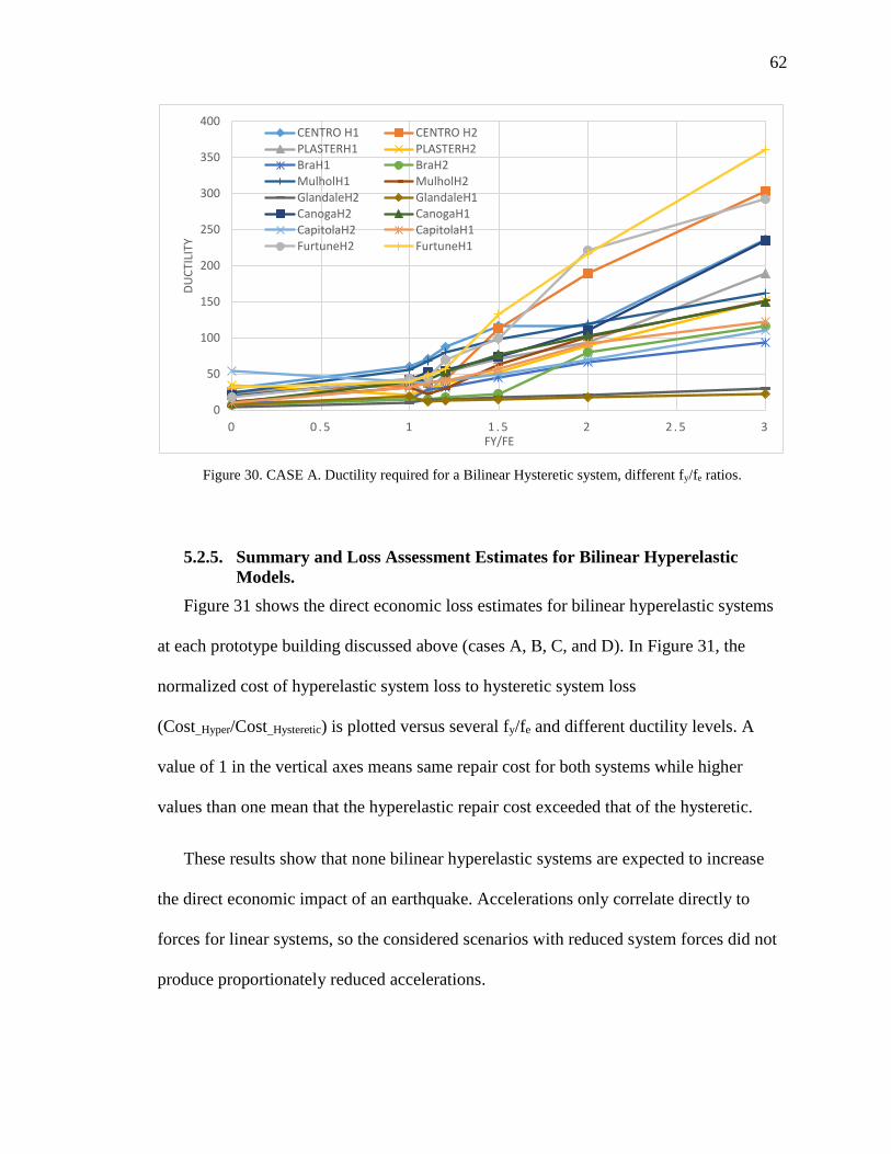
62
Figure 30. CASE A. Ductility required for a Bilinear Hysteretic system, different fy/fe ratios.
5.2.5. Summary and Loss Assessment Estimates for Bilinear Hyperelastic
Models.
Figure 31 shows the direct economic loss estimates for bilinear hyperelastic systems
at each prototype building discussed above (cases A, B, C, and D). In Figure 31, the
normalized cost of hyperelastic system loss to hysteretic system loss
(Cost_Hyper/Cost_Hysteretic) is plotted versus several fy/fe and different ductility levels. A
value of 1 in the vertical axes means same repair cost for both systems while higher
values than one mean that the hyperelastic repair cost exceeded that of the hysteretic.
These results show that none bilinear hyperelastic systems are expected to increase
the direct economic impact of an earthquake. Accelerations only correlate directly to
forces for linear systems, so the considered scenarios with reduced system forces did not
produce proportionately reduced accelerations.
0
50
100
150
200
250
300
350
400
0 0 . 5 1 1 . 5 2 2 . 5 3
DU
CTI
LITY
FY/FE
CENTRO H1 CENTRO H2PLASTERH1 PLASTERH2BraH1 BraH2MulholH1 MulholH2GlandaleH2 GlandaleH1CanogaH2 CanogaH1CapitolaH2 CapitolaH1FurtuneH2 FurtuneH1

63
Favorable relative repair costs will depend on whether or not the nonstructural
damage due to additional displacements offset the savings of preventing structural
damage and reduced accelerations. The buildings with a higher period (case B and D)
showed direct repair costs closer to the hysteretic, suggesting that for more flexible
structures with reduced elastic stiffness, a bilinear hyperelastic system could yield better
performance.
Figure 31. Loss assessment estimate for Bilinear Hyperelastic models.
5.3. Trilinear Hyperelastic Evaluations
Figure 32 shows different hyperelastic configurations contrasted against a
conventional hysteretic model. An infinite array of hyperelastic system permutations
could be considered. However, during the analysis, the pool of systems was significantly
reduced by considering only parametric combinations that result in equal or reduced force
compared to the hysteretic system (fe, max<fy). This requirement limited the valid range of
arresting stiffness (K3) considerably. As had been implemented for the bilinear

64
hyperelastic study, the same initial stiffness was used for both reference hysteretic and
hyperelastic systems.
Figure 32. Different Hyperelastic configurations (Force-Displacement)
During the analysis, it was noticed that the hyperelastic peak brace forces were
highly influenced by variations in frequency content of each motion, especially low-
frequency content. For instance, when motions that exhibit higher acceleration demands
(compared to those of the target spectrum) in the long period range were used, the
hyperelastic system required stricter parameter combinations to meet the mechanical
force level (i.e. FortuneH1, FortuneH2). On the other hand, when motions with lower
acceleration demands in the long period range (Tn>0.7s) were used, the hyperelastic
system met the hysteretic force level within a wider pool of parameters.
Δe Δemax
fe
Deflections
Bra
ce f
orc
e
K0
fy
ΔhmaxΔy
Kh0
Kh0 = K0
DUCT= μ
fe.max HYPERELASTICSYSTEM
Δe(μ-1)
α2
α2
α2
HYSTERETICSYSTEM

65
Trends were identified from an extensive parametric study, with main findings
presented below in a case by case format.
5.3.1. Trilinear, 3-Story Building, Low-Ductility (CASE D)
The analyses revealed that the arresting stiffness (K3) must be kept less than 0.1K0 to
ensure that the hyperelastic maximum brace force will be equal to or less than the
complementary hysteretic brace. An example is shown in Figure 33a, where the buckling
force in the hyperelastic system is three times less than the yielding force in the hysteretic
system (fy/fe = 3), and the ductility from buckling to the arresting stiffness is 2.5. In this
figure, the blue lines demarcate the maximum displacement and force in the reference
hysteretic system. When α2 is set higher than 0.1, all hyperelastic maximum forces
surpass the brace force of the reference hysteretic system. This happens to be true for the
majority of fy/fe ratios, but the lowest peak displacements were obtained with fy/fe ratios
close to 1.0. Similarly, it was found that ductility (Figure 33b) did not have considerable
influence in the force demand when lower fy/fe values were used (1 to 2).
Three values of α2 (0.1, 0.05, and 0.025) were evaluated for ductility values of 7
to 15 and fy/fe ratios from 1 to 6. the optimal combinations of K3 (α2) and ductility
with respect to peak force and displacement demands were:
α2= 0.1, μ=9 to have fe, max<fy for most fy/fe
α2= 0.05, μ>6 to have fe, max<fy for all fy/fe
α2= 0.025, any ductility allows that fe, max<fy for all fy/fe (but when fy/fe equals 1, μ
>7 is required)
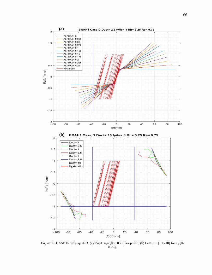
66
Figure 33. CASE D- fy/fe equals 3. (a) Right: α2= [0 to 0.25] for μ=2.5; (b) Left: μ = [1 to 10] for α2 [0-
0.25].
(a)
(b)

67
In summary, for all combinations of μ and the fy/fe ratio, the arresting stiffness (K3)
has to be less than 10% of the initial stiffness (K0). This range of stiffness was used to
meet the force limit in the brace. The best displacement responses were found when fy/fe
was closer to 1.0 (similar force level on both systems), and the highest K3 considered was
used (α2 close to 0.1).
5.3.1.1. Case D. Loss Assessment Estimates
The structural responses of hyperelastic systems with peak forces not exceeding
the comparable hysteretic system force were used to assess seismic consequences with
respect to direct building repair costs. Building accelerations and peak displacements
were mapped to direct economic loss by using the HAZUS-MH loss assessment
methodology.
Three loss estimates are presented, which provide meaningful insights about the
advantages of using either system.
Previously, it was noted that the max brace force developed in hyperelastic
systems with α2= 0.1 and μ=9 generally did not exceed the yielding force of the
reference hysteretic system (fe,max<fy for most fy/fe considered). However, when
the induced peak accelerations and displacements were mapped to direct
economic losses, only the fy/fe ratios greater than three (3) yielded considerable
savings in final repair costs (20% less than the hysteretic). This reduction is
illustrated in Figure 34, where the normalized repair cost (hyperelastic repair cost
normalized by corresponding hysteretic repair cost) is plotted against the fy/fe
ratio for several ductilities. This repair cost was compute based on the average

68
hyperelastic response obtained after running all ground motions (9 out of 16 was
the minimum number of motions needed to add a point in Figure 34).
In this figure, it is also shown that hyperelastic systems with fy/fe ratio
lower than two (2) exceeded the unity threshold, which means that such
configurations would be expected to require higher repair costs than a comparable
conventional hysteretic system.
Figure 34. CASE D- α2=0.1; Normalized repair cost, ductility, and fy/fe ratio.
Similarly, some hyperelastic systems were modeled with an α2 = 0.05 and μ>6.
Figure 35 shows that even though such systems met the force level (fe, max<fy), the
direct economic impact is not likely to be an improvement over hysteretic
systems.

69
Figure 35. CASE D- α2=0.05; Normalized repair cost, ductility, and fy/fe ratio.
Third, the loss assessment in Figure 36, showed that no hyperelastic trilinear
systems with α2= 0.025 were competitive with hysteretic systems based solely on
direct economic loss estimation.
Figure 36. CASE D- α2=0.025; Normalized repair cost, ductility, and fy/fe ratio.

70
5.3.1.2. Case D. Summary
The best hyperelastic performance was observed when the highest arresting (K3)
stiffness was used (10% of K0) because this minimized displacement demands while
brace forces were maintained similar or lower than the reference hysteretic system. This
configuration yielded a repair cost reduction of 20% over a comparable conventional
hysteretic system.
Figure 37. CASE D. (a) Acc. Vs Disp.; (b) Disp. vs. time; (c) normalized brace force vs. Displ.; (d) Acc.
vs. time.
To understand the unfavorable performance outcomes when a lower K3 was used,
the data was further examined and confirmed that the additional displacement demands
caused by the softened stiffness were not compensated by a significant reduction in
(a) (b)
(c) (d)

71
acceleration demands. Having similar damage coming from acceleration-sensitive
elements (Figure 37a, Figure 37d) and larger peak displacements (Figure 37b, Figure
37c) resulted in higher repair cost estimates for these hyperelastic systems.
Direct economic losses attributed to displacements (drift-sensitive nonstructural)
and accelerations (acceleration-sensitive nonstructural and contents) were aggregated
separately for each combination of ductility and fusing force ratio (fy/fe). The aggregated
displacement- and acceleration-based losses were then normalized by their sum for each
combination, providing a relative measure of displacement vs. acceleration demand
parameter significance. Figure 38 presents the results of these calculations for Case D at
each of α2 equal to 0.1, 0.05, and 0.025. A fy/fe ratio equal to zero (0) corresponds to the
reference hysteretic system loss distribution. Filled markers correspond to displacement-
induced damage (associated with Sd in HAZUS), and unfilled markers correspond to
acceleration-induced damage (associated with Sa in HAZUS). Structural damage was
assumed negligible for all hyperelastic models, but was included in the displacement-
based damage for the hysteretic system losses.

72
Figure 38. CASE D. (a) loss distribution for α2=0.1; (b) loss distribution for α2=0.05; (c) loss distribution
for α2=0.025.
For hyperelastic systems with low fy/fe ratios (fy/fe approaching 1, when the
hyperelastic buckling force approaches the hysteretic yielding force), the damage in the
hyperelastic structure was mainly attributable to acceleration-sensitive components (e.g.,
damaged suspended ceilings and/or mechanical, electrical, or plumbing components in
ceiling spaces, or falling shelves and damage to building contents). As the fy/fe ratio
increased, peak displacements rise correspondingly and become the primary source of
damage in the building (at drift-sensitive nonstructural elements such as partitions or
curtain walls). The damage distribution for each of the examined K3 options is shown in
(a)
(b) (c)

73
Figure 38a, Figure 38b, and Figure 38c. These figures also show that the role of ductility
diminished when systems were modeled with low α2.
5.3.2. Trilinear, 1-Story Building, Low-Ductility (CASE C)
Similarly, to the Case D building, the same initial stiffness was used for both
hysteretic and hyperelastic systems. The Case C building differs from Case D with a
shorter natural period (0.17 sec for Case C versus 0.31 sec for Case D). This building
presented a greater challenge to find hyperelastic systems that develop less or equal brace
force and comparable displacements to those of the comparable hysteretic system. These
complications were due to the excellent responses exhibited by the hysteretic model.
Testing hundreds of different hyperelastic configurations revealed that:
Systems with α2= 0.1 did not meet the force limit fe, max<fy until high ductilities
were used (μ>45). However, when the fy/fe ratio was kept below three (fy/fe <3),
ductility values as low as thirty (μ> 30) could satisfy the peak force limit.
Hyperelastic systems with α2= 0.05 required ductilities larger than twenty (μ>20)
to have fe, max<fy for all fy/fe ratios less than three (3); the rest of the fy/fe
combinations would require μ>35 to satisfy the peak force limit.
When α2= 0.025 or lower, ductilities higher than five (μ>5) are enough to
guarantee that the fe, max is less than fy. This applies to all fy/fe ratios.
5.3.2.1. Case C. Loss Assessment Estimates
HAZUS-MH estimates provided meaningful insights about the magnitudes of direct
economic loss when using hysteretic versus hyperelastic systems.

74
The analysis of hyperelastic systems with α2= 0.1, see Figure 39, shows that the
vast majority of hyperelastic models rendered higher repair costs than the
traditional hysteretic.
Figure 39. CASE C- α2=0.1; Normalized repair cost, ductility, and fy/fe ratio.
Hyperelastic systems with a α2 = 0.05 and μ>20 were evaluated. Figure 40 shows
that systems with a fy/fe ratio higher than 3 produce an estimated 10% direct
repair saving over the hysteretic model.

75
Figure 40. CASE C- α2=0.05; Normalized repair cost, ductility, and fy/fe ratio.
The loss assessment results presented in Figure 41, using α2= 0.025, showed that
increasing the flexibility generated higher total losses, while the fy/fe ratio did not
display substantial influence in either reducing or increasing direct economic loss
outcomes. In general, none of the hyperelastic systems considered were
competitive (regarding direct economic damage only) with traditional hysteretic
systems.

76
Figure 41. CASE C- α2=0.025; Normalized repair cost, ductility, and fy/fe ratio.
5.3.2.2. Case C. Summary
The most favorable hyperelastic performance relative to hysteretic performance
was observed when the arresting stiffness was set to 0.05 (5% of K0), providing a
reduction in direct economic loss of 10% over the conventional hysteretic. The rest of the
arresting stiffness, ductility and fy/fe variations considered did not result in expected
direct economic loss savings.
These adverse outcomes were further examined to find the cause of the overruns.
Figure 42 shows a representative comparison of hysteretic and hyperelastic system
responses for Case C, for one ground motion. The hyperelastic system behaved correctly,
but the reason why it was not competitive (regarding direct economic repair cost) was
due to the excellent hysteretic response that eclipsed it. The residual displacements
incurred by the hysteretic system and avoided in the hyperelastic system (structural
damage savings) were not significant enough to offset the damage caused by large

77
relative displacements (damage to nonstructural drift-sensitive elements) that result in
higher earthquake direct capital-related costs.
Figure 42. CASE C. (a) Acc. Vs Disp.; (b) Disp. vs. time; (c) normalized brace force vs. Displ.; (d) Acc. vs.
time.
Furthermore, the loss assessment distribution illustrated below (see Figure 43a)
showed that when K3 equals 10% of K0, displacement-induced and acceleration-induced
losses are approximately evenly distributed for most of the evaluated hyperelastic models
(those meeting the hysteretic mechanical force threshold). A similar loss distribution was
observed in hyperelastic systems when K3 was 5% of K0 (see Figure 43b), but a wider
pool of systems passed the force limit. Optimal combinations of fusing force ratio and
ductility produced hyperelastic systems expected to incur approximately 5% to 10% less
direct economic loss than a comparable hysteretic system.
(a)
(c) (d)
(b)

78
Systems with a shallower arresting stiffness (K3 less than 2.5% of K0) did not
provide economic savings in terms of mainshock direct economic effects. The loss
distribution (see Figure 43c) showed that most of the building damage was due to large
displacements causing the loss of nonstructural drift-sensitive elements.
Figure 43. CASE C. (a) Loss distribution for α2=0.1; (b) loss distribution for α2=0.05; (c) loss distribution
for α2=0.025.
In summary, lowering the arresting stiffness (α2) diminishes the influence of ductility
in the response. The transition to re-stiffening would not generate significant response
(a)
(b) (c)

79
variations because of the smooth change in the system stiffness (the trilinear system
approaches a bilinear response, similar to those previously analyzed in section 5.2.2).
Regarding the fy/fe ratio, when low ratios were used (fy/fe=1), the damage in the
hyperelastic structure was mainly because of acceleration-sensitive component failures.
Increasing the ratio reversed the loss distribution proportions.
5.3.3. Trilinear, 3-Story Building, High Ductility (CASE B)
As mentioned in the scope of this work, the same initial stiffness (K0=Kh0) was used
for both hysteretic and hyperelastic systems. The Case B prototype building was similar
to Case D, but designed to withstand high seismic demands with greater ductility. The
code provides a response modification factor, R, of 6 for structures with SCBFs. As
discussed in the Methodology chapter, the natural period associated with this Case was
estimated to be 0.4 sec.
As observed for Case D and C structures, hyperelastic Case B parameter evaluations
with arresting stiffness ratio, K3, greater than 10% of K0 did not meet the force limit
(equal or less elastic force than the corresponding hysteretic system). Accordingly, the
SDOF analyses conducted were limited to K3 equal 10%, 5%, and 2.5%. The main
findings for each modeled K3 value are summarized as follow:
• When K3 equals 10% of the initial stuffiness (α2 = 0.1), a ductility greater than 35
(μ>35) was required to meet the force limit (fy>fe,max) for all fy/fe ratios that complied (one
to four). However, low fy/fe ratios (1 to 1.5) complied with the force limit while rendering
lower ductility demands (μ>25). This means that for a system with a response
modification factor, R, of 6, the hyperelastic buckling force should preferably be selected

80
close to the corresponding yield force of the hysteretic system to minimize
uneconomically large structural peak displacements.
• When K3 was set equal to 5% of K0 (α2 = 0.05), parameter permutations that
included ductilities higher than 15 (μ>15) and fy/fe ratios between one and five met the
force limit.
• For the shallowest arresting stiffness analyzed, K3 equals 2.5% of K0 (α2= 0.025),
ductilities higher than 16 (μ>16) were required when fy/fe equaled one (fy=fe) to ensure
that the hyperelastic brace force will be equal to or less than the complementary
hysteretic brace. However, for higher fy/fe (2 to 5) ratios ductilities as low as five (μ>5)
secured peak mechanical forces below the threshold (fe,max<fy).
5.3.3.1. Case B. Loss Assessment Estimates
Loss assessments using the HAZUS-MH methodology were conducted for each
arresting stiffnesses noted previously (10%, 5%, and 2.5% of K0) and the results are
summarized in Figure 44, Figure 45, and Figure 46, respectively.
The analyses indicated that none of the hyperelastic systems discussed above would
reduce the cost of replacing nonstructural and contents elements. Despite the savings
from structural system protection, the repair cost would rise to around 20% over the
traditional hysteretic.

81
Figure 44. CASE B- α2=0.1; Normalized repair cost, ductility, and fy/fe ratio.
Figure 45. CASE B- α2=0.05; Normalized repair cost, ductility, and fy/fe ratio.

82
Figure 46. CASE B- α2=0.025; Normalized repair cost, ductility, and fy/fe ratio.
5.3.3.2. Case B. Summary
Most of the hyperelastic systems that rendered less or equal peak force demand than
the hysteretic system (fe,max<fy) did not produce direct economic loss reductions.
However, in Figure 45, there was a single hyperelastic system that produced a lower
repair cost than that of the hysteretic system. This system has a ductility of 24 and a fy/fe
ratio of 1 (fy=fe). Analyzing the only beneficial response may help to understand why the
rest that were examined failed. Figure 48 presents response plots for a single ground
motion. In Figure 47b, the hysteretic system experienced a large permanent displacement
(Δhmax>100 mm, 3.93 in), while there were not significant differences regarding peak
accelerations (Figure 48a). Furthermore, the loss distribution plot (see Figure 49b)
showed that when fe is set to equal fy, the vast majority of damage comes from
acceleration-sensitive elements. Based on this scenario, this particular hyperelastic
system saves 10% in repair costs over the hysteretic, because the structural damage was
avoided while damage to acceleration-sensitive elements was comparable.

83
Figure 47. CASE B. (a) Acc. Vs Disp.; (b) Disp. vs. time; (c) normalized brace force vs. Displ.; (d) Acc. vs.
time.
The loss distribution analysis illustrated by Figure 48 shows that for all systems,
the loss of drift-sensitive elements accounted for most of the damage for all systems
evaluated (independently of the K3, fy/fe ratio, and ductility).
(a) (b)
(c) (d)

84
Figure 48. CASE B. (a) Loss distribution for α2=0.1; (b) loss distribution for α2=0.05; (c) loss distribution
for α2=0.025.
5.3.4. Trilinear, 1-Story Building, High Ductility (Case A).
Similar to previous cases, three values of α2 were evaluated (0.1,0.05, and 0.025) for
all ductility and fy/fe variations that rendered superior or competitive peak responses to
that of the reference hysteretic. After extensive parameter changes, the optimal
combinations of K3 (α2), ductility, and hyperelastic peak force (fe, max) are:
(a)
(c) (b)

85
For α2= 0.1, a ductility higher than sixty (μ>60) is required to meet the force limit,
only fy/fe ratios between 1 to 1.5 passed the force limit criterion. Furthermore,
systems equipped with lower fy/fe ratios met the hysteretic force threshold with
lower ductility demands (μ>45). Regarding peak displacements, the closer fe was
to fy, the better.
For systems with α2= 0.05, ductilities higher than forty-five were needed (μ>45)
to ensure that fe, max<fy. This was true for fy/fe ratios between 1 and 1.3. For fy/fe
ratios between 1.3 and 1.5, a ductility higher than sixty (μ>60) was needed to
ensure that fe, max remained below fy. Higher fy/fe ratios than 1.5 did not meet the
force limit criterion.
For hyperelastic configurations with α2= 0.025, μ>45 allowed that fe, max<fy for all
fy/fe ratios between 1 to 1.5. Higher fy/fe ratios did not meet the force cap.
5.3.4.1. Case A. Loss Assessment Estimates
For this building (case A, R = 6, Tn = 0.2 sec), the loss assessment estimates
conducted using HAZUS-MH are shown in Figure 49, Figure 50, and Figure 51, where α2
equals 0.1, 0.05, and 0.025%, respectively. These analyses indicated that implementing
none of the above hyperelastic systems would produce reductions in repair costs.
Conversely, they would increase direct economic loss up to 40%.

86
Figure 49. CASE A- α2=0.1; Normalized repair cost, ductility, and fy/fe ratio.
Figure 50. CASE A- α2=0.5; Normalized repair cost, ductility, and fy/fe ratio.
Figure 51. CASE A- α2=0.025; Normalized repair cost, ductility, and fy/fe ratio.

87
5.3.4.2. Case A. Summary
None of the examined hyperelastic systems produced direct economic loss savings.
Even though hyperelastic systems had a lower peak force than that of the hysteretic
reference model (fe,max<fy), the accelerations reached by the hyperelastic system were
equal or even higher to those in the hysteretic (see Figure 52a). Furthermore, the loss
distribution shown in Figure 53 proves that displacement-induced damage constituted
most of the total building loss. Therefore, avoiding structural damage by incorporating
the hyperelastic fuse was not enough to render repair cost savings.
Figure 52. CASE A. (a) Acc. Vs Disp.; (b) Disp. vs. time; (c) normalized brace force vs. Displ.; (d) Acc.
vs. time.
(d)
(a) (b)
(c)

88
Figure 53. CASE A. (a) Loss distribution for α2=0.1; (b) loss distribution for α2=0.05; (c) loss distribution
for α2=0.025.
(c) (b)
(a)

89
CHAPTER 6. CONCLUSIONS
Findings related to economic loss were drawn solely based on HAZUS direct
economic loss assessments. HAZUS guidelines and procedures were developed by a team
of earthquake loss experts, including earth scientists, engineers, architects, economists,
emergency planners, social scientists, and software developers. (Schneider and Schauer
2006)
6.1. Case Specific
6.1.1. CASE D. (3 stories, R=3.1/4)
In comparison with its hysteretic equivalent, the best trilinear hyperelastic
performance rendered an average 20% total loss reduction to mitigate earthquake
mainshock’s effects.
The buckling force of the slender elements must be three to six times less than the
comparable hysteretic yielding force, while the gap of the fuse should remain
within six to nine times the displacement corresponding to slender fusing element
elastic buckling.
Displacements were the primary source of damage for the hyperelastic models.
Conversely, accelerations accounted for most of the direct economic loss in the
reference hysteretic system.
6.1.2. CASE C (1 story, R=3.1/4)
The trilinear hyperelastic alternative rendered an average 10% reduction of the
direct repair cost (response to mainshock only).

90
The buckling force of the slender elements must be three to six times lesser than
the comparable hysteretic yielding force, while the gap of the fuse should remain
within 19 to 39 times the buckling displacement of the slender elements.
Displacements and accelerations contributed evenly to the final loss estimates for
the hyperelastic system. On the other hand, the hysteretic direct loss was 85% due
to acceleration-induced damage.
6.1.3. CASE B (3 stories, R=6)
None of the hyperelastic parametric combinations having equal or reduced
force compared to the hysteretic system produce reductions in mainshock
direct economic loss. Alternative, multi-linear, hyperelastic combinations may
reduce accelerations demands and thus reduce hyperelastic repair cost.
Displacements are the primary source of damage for all hyperelastic systems as
well as for the reference hysteretic.
6.1.4. CASE A (1-Story Building, High Ductility)
None of the included trilinear hysteretic models rendered mainshock
reparability savings. The accelerations reached were equal or higher, while the
displacements were larger than the reference hysteretic system. Therefore, the
advantages of using hyperelastic systems in this scenario are reduced to
aftershock resistance to prevent casualties and reduced indirect economic and
social impacts.
Displacements were the primary source of damage (for hysteretic and
hyperelastic models).
91
6.2. General
Loss assessments for nominally comparable hysteretic systems were premised on
full hysteresis under cyclic loading. However, OCBF and SCBF systems are
expected to exhibit pinched hysteresis associated with global buckling of the
brace between the end connections. The modeled hysteretic behavior is more
representative of a buckling-restrained brace (BRB) system than a CBF system.
Therefore, the loss estimates for hysteretic systems were unconservative (higher
losses should be expected), which led to hysteretic-to-hyperelastic comparisons
unfairly favorable to hysteretic systems.
Loss assessment estimations for all prototype buildings discussed above (cases A,
B, C, and D) provided with bilinear hyperelastic systems showed that none of
such bilinear hyperelastic systems would produce reductions in repair costs. The
results highlighted that reducing the peak mechanical force does not guarantee
proportionate reductions in the system accelerations.
Analyses of the considered trilinear hyperelastic systems suggested that the
arresting stiffness (K3) should generally remain below 10% of the initial stiffness
(K0) to prevent hyperelastic system maximum LFRS forces from exceeding the
force demands for comparable hysteretic systems. Additionally, lowering the
arresting stiffness diminishes the influence of ductility in the response. The
transition to re-stiffening would not generate significant response variations
because of the smooth change in the system stiffness (the trilinear system
approaches a bilinear response). The fusing force ratio (ratio of hysteretic yield to

92
hyperelastic buckling, fy/fe) was the most important parameter, because it was
strongly correlated to the peak displacement demands.
The mainshock response of hysteretic stiff systems (low period) was outstanding.
Therefore, more complex hyperelastic systems (i.e. more than two post-buckling
stiffness [staircase]) should be explored to enhance reparability outcomes.
Generally, for stiff systems, the hyperelastic savings from avoiding structural
damage were not enough to offset drift-sensitive nonstructural losses.
6.3. Future Research Needs and Opportunities
Hyperelastic systems will commonly display more flexible responses than those
of conventional hysteretic structures. Therefore, their effectiveness could be
highly dependent on site condition (stiff, dense, rock) and the interdependency
of site motion and hyperelastic response.
Second order effects (P-Δ) were not explicitly considered in this study.
Additional studies accounting for full material and geometric nonlinearity are
required to investigate the degree to which P-Δ may influence expected
hyperelastic system performance.
Additional studies should be performed to examine the relative performance
outcomes across wider dimensions than addressed in this thesis. The study in this
thesis was limited to direct economic loss (repair and replacement costs for
structural, nonstructural, and contents). Hysteretic systems are susceptible to
permanent deformations after inelastic excursions, whereas hyperelastic systems
will return to the original configuration. This potential difference in residual

93
structure configuration can lead to indirect economic loss and social impacts due
to interrupted occupancy and operational functionality that were not within the
scope of this thesis, as well as susceptibility to aftershocks.
The spectrum of possible hyperelastic systems using a controlled elastic-
buckling mechanism is infinite, and more complex multi-linear hyperelastic
systems could render better responses. For instance, it may be worth exploring
various initial stiffnesses (K0), or fuses with multiple buckling levels, in which
slender elements with different lengths are strategically arranged to produce a
staircase force-displacement response. Additionally, the medium in which the
slender elements of the fuse displace once they have buckled could be modified
to add damping and dissipate energy (e.g., exchange air for a denser fluid).
94
CHAPTER 7. REFERENCES
Ancheta, T. D., Darragh, R. B., Stewart, J. P., Seyhan, E., Silva, W. J., Chiou, B. S. J.,
Wooddell, K. E., Graves, R. W., Kottke, A. R., Boore, D. M., Kishida, T., and
Donahue, J. L. (2013). “PEER NGA-West2 Database.”
ASCE/SEI. (2010). ASCE/SEI 7-10 Minimum Design Loads for Buildings and Other
Structures. ASCE/SEI 7-10 Minimum Design Loads for Buildings and Other
Structures.
Chopra, A. K. (2012). Dynamics of Structures Theory and Applications to Earthquake
Engineering. ( holly stark, ed.), pearson.
Christopoulos, C., Tremblay, R., Kim, H.-J., and Lacerte, M. (2008). “Self-Centering
Energy Dissipative Bracing System for the Seismic Resistance of Structures:
Development and Validation.” Journal of Structural Engineering, 134(1), 96–107.
Clifton, C., Bruneau, M., Macrae, G., Leon, R., and Fussell, A. (2011). No Title. Bulletin
of the New Zealand Society for Earthquake Engineering.
Cook, J., Rodgers, G. W., Macrae, G. A., and Chase, J. G. (2015). “Development of a
ratcheting , tension-only fuse mechanism for seismic energy dissipation.”
Erochko, J., and Christopoulos, C. (n.d.). “Self-Centering Energy-Dissipative (SCED)
Brace: Overview of Recent Developments and Potential Applications for Tall
Buildings.”
Erochko, J., and Christopoulos, C. (2014). “Self-centering energy-dissipative (SCED)
Brace: Overview of recent developments and potential applications for tall
buildings.” Sustainable Development of Critical Infrastructure - Proceedings of the
2014 International Conference on Sustainable Development of Critical
95
Infrastructure, 488–495.
FEMA. (2000). “Seismic design criteria for new moment-resisting steel frame
construction, Report No. FEMA 350.” 221.
FEMA. (2015). “Hazus–MH 2.1: Technical Manual.” National Institute of Building
Sciences and Federal Emergency Management Agency (NIBS and FEMA), 718.
Gao, N., Jeon, J.-S., Hodgson, D. E., and DesRoches, R. (2016). “An innovative seismic
bracing system based on a superelastic shape memory alloy ring.” Smart Materials
and Structures, IOP Publishing, 25(5), 55030.
Goldsworthy, H. M. (2012). “Lessons on building design from the 22 February 2011
Christchurch earthquake.” Australian Journal of Structural Engineering, 13(2),
159–174.
Hajjar, J. F., Sesen, A. H., Jampole, E., and Wetherbee, A. (2013). “Rocking , Self-
Centering , and Articulated Energy- Dissipating Fuses.” Journal of Earthquake
Engineering, 10(1), 45–66.
Hashemi, A., Zarnani, P., Masoudnia, R., and Quenneville, P. (2017). “Seismic resistant
rocking coupled walls with innovative Resilient Slip Friction (RSF) joints.” Journal
of Constructional Steel Research, Elsevier Ltd, 129, 215–226.
Kircher, C. a., Whitman, R. V., and Holmes, W. T. (2006). “HAZUS Earthquake Loss
Estimation Methods.” Natural Hazards Review, 7(2), 45–59.
Malley, J. O., Popov, E. P., and Asce, F. (n.d.). “SHEAR LINKS IN ECCENTRICALLY
BRACED FRAMES.”
McCormick, J., DesRoches, R., Fugazza, D., and Auricchio, F. (2007). “Seismic
assessment of concentrically-braced steel frames with shape memory alloy braces.”

96
Journal of Structural Engineering-Asce, 133(6), 862–870.
Patro, S., and Sinha, R. (2008). “Optimal seismic performance of friction energy
dissipating devices.” The 14th World Conference on ….
Qiu, C. X., and Zhu, S. (2017a). “Performance-based seismic design of self-centering
steel frames with SMA-based braces.” Engineering Structures, 130, 67–82.
Qiu, C., and Zhu, S. (2017b). “Shake table test and numerical study of self-centering steel
frame with SMA braces.” Earthquake Engineering and Structural Dynamics.
Rahimatpure, A. (2012). “Smart Memory Alloys.” 118–120.
Rodriguez-Nikl, T. (2015). “Linking disaster resilience and sustainability.” Civil
Engineering and Environmental Systems, 32(1–2), 157–169.
Roeder, C. W., and Popov, E. P. (1978). “Eccentrically Braced Steel Frames for
Earthquakes.” Journal of the Structural Division, 104(3), 391–412.
Schneider, P. J., and Schauer, B. A. (2006). “HAZUS—Its Development and Its Future.”
Natural Hazards Review, 7(2), 40–44.
Stevenson, J., Kachali, H., Whitman, Z., Seville, E., Vargo, J., and Wilson, T. (2011).
“Preliminary Observations of the Impacts the 2nd February Christchurch Earthquake
had on Organisations and the Economy: A Report from the Field.” Bulletin of the
New Zealand Society for Earthquake Engineering, 44(2).
Taghavi, Shahram; Miranda, E. (2004). “13 th World Conference on Earthquake
Engineering ESTIMATION OF THE DYNAMIC PROPERTIES FOR
GEOSYNTHETIC INTERFACES.” Program.
Tremblay, R., Lacerte, M., and Christopoulos, C. (2008). “Seismic Response of
Multistory Buildings with Self-Centering Energy Dissipative Steel Braces.” Journal

97
of Structural Engineering, 134(1), 108–120.
USGS. (2015). “Design Maps Site D-Stiff Soil.” 1–9.
Vargas, R., and Bruneau, M. (2005). “Investigation of the Structural Fuse Concept.”
Draft Report.
Vargas, R., and Bruneau, M. (2009). “Analytical Response and Design of Buildings with
Metallic Structural Fuses. I.” Journal of Structural Engineering, 135(4), 386–393.