Hyper-sparsity in the revised simplex

method and how to exploit it

J. A. J. Hall K. I. M. McKinnon

08th

October 2002

Abstract

The revised simplex method is often the method of choice whensolving large scale sparse linear programming problems, particularly whena family of closely-related problems is to be solved. Each iteration ofthe revised simplex method requires the solution of two linear systemsand a matrix vector product. For a significant number of practicalproblems the result of one or more of these operations is usually sparse, aproperty we call hyper-sparsity. Analysis of the commonly-used techniquesfor implementing each step of the revised simplex method shows themto be inefficient when hyper-sparsity is present. Techniques to exploithyper-sparsity are developed and their performance is compared with thestandard techniques. For the subset of our test problems that exhibitshyper-sparsity, the average speedup in solution time is 5.2 when thesetechniques are used. For this problem set our implementation of therevised simplex method which exploits hyper-sparsity is shown to becompetitive with the leading commercial solver and significantly fasterthan the leading public-domain solver.

1 Introduction

Linear programming (LP) is a widely applicable technique both in its own rightand as a sub-problem in the solution of other optimization problems. Therevised simplex method and the barrier method are the two efficient methodsfor solving general large sparse LP problems. In a context where families ofrelated LP problems have to be solved, such as in integer programming anddecomposition methods, the revised simplex method is usually the more efficientmethod.

The constraint matrices for most practical LP problems are sparse and, foran implementation of the revised simplex method to be efficient, it is crucialthat only non-zeros in the coefficient matrix are stored and operated on. Eachiteration of the revised simplex method requires the solution of two linearsystems, the computation of which are commonly referred to as FTRAN andBTRAN, and a matrix vector product computed as the result of an operationreferred to as PRICE. The matrices involved in these operations are submatricesof the coefficient matrix so are normally sparse. For many problems these threeoperations yield dense vectors, in which case there is limited scope for improvingthe performance by fully exploiting any zeros in the vectors. However, there is

1

a significant number of practical problems where the results of one or moreof these operations are usually sparse, a property referred to in this paper ashyper-sparsity. This phenomenon has been reported independently by Bixby [3]and Bixby et al [4]. A number of classes of problems are known to exhibithyper-sparsity, in particular those with a significant network structure suchas multicommodity flow problems. Specialist variants of the revised simplexmethod which exploit this structure explicitly have been developed, in particularby McBride and Mamer [16, 17]. This paper identifies hyper-sparsity in awider range of more general LP problems. Techniques are developed whichcan be applied within a general revised simplex solver when hyper-sparsityis identified during the solution process and, for problems exhibiting hyper-sparsity, significant performance improvements are demonstrated.

The computational components of the revised simplex method and standardtechniques for FTRAN and BTRAN are introduced in Section 2 of this paper.Section 3 describes hyper-sparsity and gives statistics on its occurrence in atest set of LPs drawn from the standard Netlib set [10], the Kennington testset [5] and the authors’ personal collection [13]. Analysis given in Section 4shows the commonly-used techniques for each of the computational componentsof the revised simplex method to be inefficient when hyper-sparsity is presentand techniques to exploit hyper-sparsity are described. Section 5 presents acomputational comparison of the authors’ revised simplex solver, EMSOL, withand without the techniques for exploiting hyper-sparsity. For those problemswhich exhibit hyper-sparsity, a comparison is also made between EMSOL,SOPLEX 1.2 [21] and the CPLEX 6.5 [15] primal simplex solver. Conclusionsare offered in Section 6.

Although it contains no new ideas, this paper represents a significantreworking of [12]. The presentation has been greatly improved and thecomparisons between EMSOL, SOPLEX and CPLEX have been added.

2 The revised simplex method

The revised simplex method and its computational requirements are mostconveniently discussed in the context of LP problems in standard form

minimize cT xsubject to Ax = b

x ≥ 0,

where x ∈ IRn and b ∈ IRm.In the simplex method, the variables are partitioned into index sets B of

m basic variables and N of n − m nonbasic variables such that the basismatrix B formed from the columns of A corresponding to the basic variablesis nonsingular. The set B itself is conventionally referred to as the basis. Thecolumns of A corresponding to the nonbasic variables form the matrix N and thecomponents of c corresponding to the basic and nonbasic variables are referred toas, respectively, the basic costs cB and non-basic costs cN . When the nonbasicvariables are set to zero the values b = B−1b of the basic variables, if non-negative, correspond to a vertex of the feasible region. If any basic variablesare infeasible they are given costs of −1, with other variables being given costsof zero. Phase I iterations are then performed in order to force all variables to

2

be non-negative, if possible. An account of the details of the revised simplexmethod is given by Chvatal in [6] and the computational components of eachiteration are summarised in Figure 1. Note that although the reduced costs maybe computed directly using the following BTRAN and PRICE operations

πTB = cT

BB−1

cTN = cT

N − πTBN,

it is more efficient computationally to update them by calculating the pivotalrow aT

p = eTp B−1N , where ep is column p of the identity matrix, using

the BTRAN and PRICE operations defined in Figure 1. The only significantcomputational requirement which is not indicated in Figure 1 occurs when, in aphase I iteration, one or more variables which remain basic become feasible sotheir cost coefficients increase by one to zero. In order to update the reducedcosts, it is necessary to compute the corresponding linear combination of tableaurows. This composite row is formed by the following BTRAN and PRICE

operationsπT

δ = δT B−1

aTδ = πT

δ N,

where the nonzeros in δ are equal to one for each variable which remainsbasic and becomes feasible. In this paper, techniques are discussed which areapplicable to all BTRAN and PRICE operations. This is done with reference toan unsubscripted vector π corresponding to a generic right-hand-side vectorr for the system B0

T π = r solved by BTRAN. When techniques are onlyapplicable to a particular class of BTRAN or PRICE operations, the specificnotation for the right-hand-side and solution is used.

CHUZC: Scan cN

for a good candidate q to enter the basis.FTRAN: Form the pivotal column aq = B−1aq, where aq is column q of A.CHUZR: Scan the ratios bi/aiq for the row p of a good candidate to leave the

basis. Let α = bp/apq.Update b := b − αaq.

BTRAN: Form πTp = eT

p B−1.PRICE: Form the pivotal row aT

p = πTp N .

Update reduced costs cTN := cT

N − cqaTp .

If (growth in factors) thenINVERT: Form a factored representation of B−1.

elseUPDATE: Update the factored representation of B−1 corresponding to the

basis change.end if

Figure 1: Operations in an iteration of the revised simplex method

Efficient implementations of the revised simplex method generally weighteach reduced cost in CHUZC by some measure of the magnitude of thecorresponding column of the standard simplex tableau, commonly referred toas an edge weight. Many solvers, including the authors’ solver EMSOL, usethe Harris Devex strategy [14]. This requires only the pivotal row to update

3

the edge weights so carries no significant computational overhead beyond thatoutlined in Figure 1.

2.1 The representation of B−1

In each iteration of the simplex method it is necessary to solve two systems,one involving the current basis matrix B and the other its transpose. Thisis achieved by passing respectively forwards and backwards through the datastructure corresponding to a factored representation of B−1. There are a numberof procedures for updating the factored representation of B−1, the original andsimplest being the product form update of Dantzig and Orchard-Hays [7]. Thisapproach is used by EMSOL and the techniques in this paper are developedwith the product form update in mind.

If B−10 is used to denote the factored representation obtained by INVERT,

and EU represents the transformation of B0 corresponding to subsequent basischanges such that B = B0EU , it follows that B−1 may be expressed as

B−1 = E−1U B−1

0 .

In a typical implementation of the revised simplex method for large sparse LPproblems, B−1

0 is represented as a product of KI elimination operations deriveddirectly from the nontrivial columns of the matrices L and U which form anLU decomposition of (a row and column permutation of) B0. This invertiblerepresentation allows B−1

0 to be expressed algebraically as B−10 =

∏1k=KI

E−1k ,

where

E−1k =

1 −ηk1

. . ....

1 −ηkpk−1

1−ηk

pk+1 1...

. . .−ηk

m 1

1. . .

1µk

1. . .

1

. (1)

Within an implementation, the nonzeros in the ‘eta’ vector

ηk = [ ηk1 . . . ηk

pk−1 0 ηkpk+1 . . . ηk

m ]T

are stored as value-index pairs and the data structure {pk, µk, ηk}KI

k=1 is referredto as an eta file. Eta vectors associated with the matrices L and U coming fromGaussian elimination are referred to as L-etas and U -etas respectively. Note thatthe number of nonzeros in the eta file is no more that the number of nonzerosin the LU decomposition.The operations with pk, µk and ηk required whenforming E−1

k r during the standard algorithms for FTRAN and E−Tk r during

BTRAN are illustrated in Figure 2.The product form update leaves the factored form of B−1

0 unaltered andrepresents E−1

U as a product of pairs of elementary matrices of the form (1).The representation of each UPDATE operation is obtained directly from thepivotal column and is given by pk = p, µk = 1/apq and ηk = aq − apqep.

In solvers based on the product form, the representation of the UPDATE

operations can be appended to the eta file following INVERT, resulting in a

4

if (rpk6= 0) then

rpk:= µkrpk

r := r − rpkηk

end if

(a) FTRAN

rpk:= µk(rpk

− rT ηk)

(b) BTRAN

Figure 2: Standard operations in FTRAN and BTRAN

single homogeneous data structure. However, in this paper and in EMSOL,the particular properties of the INVERT and UPDATE etas and the nature ofthe operations with them are exploited, so FTRAN is performed as the pair ofoperations

aq = B−10 aq (I-FTRAN)

followed byaq = E−1

U aq. (U-FTRAN)

Conversely, BTRAN is performed as

πT = rT E−1U

(U-BTRAN)

followed byπT = πT B−1

0 . (I-BTRAN)

Note that the term RHS is used to refer, not just to the vector on the right handside of the system to be solved, but to the vector at any stage in the process oftransforming it into the solution of the system.

3 What is hyper-sparsity?

Each iteration of the revised simplex method performs FTRAN to obtain thepivotal column aq = B−1aq as the solution of one linear system, BTRAN toobtain πT

p = eTp B−1 as the solution of a second linear system, and PRICE

to form the pivotal row aTp = πT

p N as the result of a matrix-vector product.For many LP problems, even those for which the constraint matrix is sparse,there are few zero values in the results of these operations. However, as thispaper demonstrates, there is a significant set of practical problems for which theproportion of zero values in the results of these operations is such that exploitingthis yields very large computational savings.

For the sake of classifying test problems, in this paper the result of anFTRAN, BTRAN or PRICE operation is considered to be sparse if no morethan 10% of its entries are nonzero and if at least 60% of the results of thatparticular operation are sparse then this is taken to be a clear majority. An LPproblem is considered to exhibit hyper-sparsity if a clear majority of the resultsof one or more of these operations is sparse. These thresholds are used for thepresentation of results only and are not parameters in the implementation ofthe methods which exploit hyper-sparsity.

The extent to which hyper-sparsity exists in LP problems was investigatedfor a subset of the standard Netlib test set [10], the Kennington test set [5]

5

and the authors’ personal collection [13]. Those problems from the Netlib setwhose solution requires less than ten seconds of CPU time were excluded, aswere FIT2D and the OSA problems from the Kennington set. For the latterproblems, the number of columns is particularly large relative to the number ofrows so the the solution techniques developed in this paper are inappropriate.Note that a simple standard scaling algorithm is applied to each of the problemsfor reasons of numerical stability and each problem is solved from the initial basisobtained using the crash procedure in CPLEX [15].

For each problem the density of each pivotal column aq following FTRAN, ofπp and πδ following BTRAN and of aT

p and aTδ following PRICE was determined,

and the total number of each which was found to be sparse was counted. Theproblems for which there is a clear majority of sparse results for at least one ofthese three operations are listed in Table 1 and referred to as test set H. Theremaining problems, those which exhibit no hyper-sparsity in any of FTRAN,BTRAN or PRICE, are listed in Table 2 and referred to as test set H′. Foreach of the three operations, Tables 1 and 2 give the percentage of the resultswhich are sparse. Subsequent columns give, for each of the three operations,the average density of those results which are sparse and the average density ofthose results which are not. The final column of Table 1 summarises the extentto which the problem exhibits hyper-sparsity by giving the initial letter of theoperation(s) for which a clear majority of the results is sparse.

The first thing to note from the results in Table 1 is that all but two of theproblems in H exhibit hyper-sparsity for BTRAN and most do so for all threeoperations. It is interesting to consider why this is the case and why there areexceptions.

Recall that the result of FTRAN is the pivotal column aq and the resultof (most) PRICE operations is the pivotal row. Since these are a column androw from the same matrix (the standard simplex tableau B−1N) it might beexpected that a problem would exhibit hyper-sparsity in both FTRAN andPRICE or in neither. Also, since the πp is just a single row of B−1, and thepivotal column is usually a linear combination of several columns of B−1, itmight be expected that πp would be less dense than aq. These arguments wouldlead us to expect all problems in H to have property B, and that problems in Hwould be either FBP or B. The reasons for the exceptions are now explained.

There are two problems, DCP1 and DCP2, of type F, i.e. the pivotal columnsare typically sparse but the results of BTRAN and PRICE are not. Theseproblems are decentralised planning problems for which a typical standardsimplex tableau is very sparse with a few dense rows. Thus the pivotal columnsare usually sparse. However, the pivot is usually chosen from one of the denserows.

Conversely there are five problems of the opposite type, BP, i.e. the pivotalrows are typically sparse but the pivotal columns are not. The most remarkableof these is FIT2P: 81% of pivotal columns are essentially full and all but one ofthe pivotal rows are sparse. For this problem, most columns of the constraintmatrix have only one nonzero entry, with the remaining columns being verydense. Thus B−1 is largely diagonal with a small number of essentially fullcolumns. For this model it turns out that most variables chosen to enter thebasis have a single nonzero entry such that the pivotal column is (a multiple of)one of these dense columns of B−1. Each πp is a row of B−1 and its resulting

6

Mean density (%)Dimensions Sparse results (%) Sparse results Non-sparse results Hyper-

Problem Rows Columns Nonzeros FTRAN BTRAN PRICE FTRAN BTRAN PRICE FTRAN BTRAN PRICE sparse80BAU3B 2262 9799 21002 97 72 70 2.40 0.61 0.66 10.84 42.41 50.85 FBPFIT2P 3000 13525 50284 19 100 100 0.17 0.65 0.91 91.10 16.93 19.46 BPGREENBEA 2392 5405 30877 15 60 60 4.62 0.49 0.81 24.73 75.54 80.75 BPGREENBEB 2392 5405 30877 16 61 60 4.55 0.48 0.77 27.81 77.75 83.78 BPSTOCFOR3 16675 15695 64875 29 100 75 2.09 2.26 2.86 62.18 — 14.97 BPWOODW 1098 8405 37474 32 73 71 3.90 1.01 1.14 22.60 57.55 59.91 BPDCP1 4950 3007 93853 98 56 47 4.52 1.33 1.26 11.00 13.90 82.60 FDCP2 32388 21087 559390 100 59 53 1.25 0.68 0.45 — 15.08 82.34 FCRE-A 3516 4067 14987 100 82 80 1.91 0.39 0.61 — 28.17 56.06 FBPCRE-C 3068 3678 13244 100 83 80 2.86 0.45 0.59 — 33.71 58.43 FBPKEN-11 14694 21349 49058 100 98 97 0.10 0.27 0.28 — 11.88 13.79 FBPKEN-13 28632 42659 97246 100 92 92 0.12 0.16 0.17 — 35.85 42.07 FBPKEN-18 105127 154699 358171 100 93 93 0.05 0.21 0.20 — 39.58 41.94 FBPPDS-06 9881 28655 62524 100 97 97 0.94 0.34 0.46 — 18.95 17.71 FBPPDS-10 16558 48763 106436 100 96 96 1.22 0.24 0.31 — 23.60 25.19 FBPPDS-20 33874 105728 230200 100 94 94 2.55 0.21 0.29 — 41.87 41.11 FBP

Table 1: Problems exhibiting hyper-sparsity (set H): dimensions, percentage of the results of FTRAN, BTRAN and PRICE which aresparse, average density of those results which are sparse, average density of those results which are not and summary of those operationsfor which more than 60% of the results are sparse.

7

Mean density (%)Dimensions Sparse results (%) Sparse results Non-sparse results

Problem Rows Columns Nonzeros FTRAN BTRAN PRICE FTRAN BTRAN PRICE FTRAN BTRAN PRICE

BNL2 2324 3489 13999 29 36 35 2.28 0.61 0.79 28.56 40.03 70.22D2Q06C 2171 5167 32417 12 25 25 1.84 0.48 0.86 49.32 66.32 87.24D6CUBE 415 6184 37704 2 9 9 5.10 0.64 1.11 65.98 94.43 97.91DEGEN3 1503 1818 24646 15 43 42 4.42 1.22 1.47 25.55 62.05 84.97DFL001 6071 12230 35632 2 37 37 1.57 0.22 0.37 51.57 83.45 92.51MAROS-R7 3136 9408 144848 24 1 1 0.54 0.59 1.43 81.25 30.78 62.30PILOT 1441 3652 43167 9 27 24 3.89 1.59 2.06 60.86 76.31 88.51PILOT87 2030 4883 73152 8 19 15 1.33 0.99 0.89 74.93 72.50 91.08QAP8 912 1632 7296 0 11 11 1.46 0.55 1.92 83.92 75.51 98.45TRUSS 1000 8806 27836 8 39 38 4.03 0.81 1.28 47.71 85.56 80.62CRE-B 9648 72447 256095 58 55 55 4.15 0.19 0.37 14.01 55.81 89.16CRE-D 8926 69980 242646 57 56 55 3.61 0.22 0.39 13.82 54.43 89.20

Table 2: Problems not exhibiting hyper-sparsity (set H′): dimensions, percentage of the results of FTRAN, BTRAN and PRICE which aresparse, average density of those results which are sparse and average density of those results which are not.

8

sparsity is inherited by the pivotal row since most columns of N in the PRICE

operation have only one nonzero entry.Several observations can be made from the columns in Tables 1 and 2.

For those problems in H′ the density of the majority of results is such thatthe techniques developed for hyper-sparsity are seen to be of limited value.For the problems in H, those results which are not sparse may have a veryhigh proportion of nonzero entries. It is important therefore that techniquesfor exploiting hyper-sparsity are ‘switched off’ when such cases are identifiedduring a particular FTRAN, BTRAN or PRICE operation. If this is not donethen any computational savings obtained when exploiting hyper-sparsity maybe compromised.

4 Exploiting hyper-sparsity

Each computational component of the revised simplex method either forms,or operates with, the result of FTRAN, BTRAN or PRICE. Each of thesecomponents is considered below and it is shown that typical computationaltechniques are inefficient in the presence of hyper-sparsity. In each case,equivalent computational techniques are developed which exploit hyper-sparsity.

4.1 Relative cost of computational components

Table 3 gives, for test set H, the percentage of solution time which can beattributed to each of the major computational components in the revisedsimplex method. This allows the value of exploiting hyper-sparsity in aparticular component to be assessed. Although PRICE and CHUZC togetherare dominant for most problems, each of the other computational components,with the exception of I-FTRAN and I-BTRAN, constitute at least 10% of thesolution time for some of the problems. Thus, to obtain general improvementin computational performance requires hyper-sparsity to be exploited in allcomputational components of the revised simplex method.

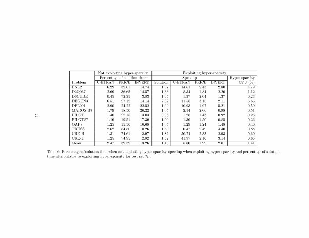
For the problems in test set H′, only U-BTRAN, PRICE and INVERT benefitnoticeably from the techniques developed below. The percentages of the solutiontime for these computational components are given as part of Table 6.

4.2 Hyper-sparse FTRAN

For most problems which exhibit hyper-sparsity, Table 3 shows that thedominant computational cost of FTRAN is I-FTRAN, particularly so for thelarger problems. When the pivotal column aq computed by FTRAN is sparse,only a very small proportion of the INVERT (and UPDATE) eta vectors, needsto be applied (unless there is an improbable amount of cancellation). Indeed thenumber of floating point operations required to perform these few operationscan be expected to be of the same order as the number of nonzeros in aq. Gilbertand Peierls [11] identified this property in the context of Gaussian eliminationwhen the pivotal column is formed as required and is expected to be sparse.It follows that the cost of I-FTRAN (and hence FTRAN) will be dominated bythe test for zero if the INVERT etas are applied using the standard operationillustrated in Figure 2(a).

9

Solution Percentage of solution timeProblem CPU (s) CHUZC I-FTRAN U-FTRAN CHUZR I-BTRAN U-BTRAN PRICE INVERT

80BAU3B 31.51 20.26 5.52 0.65 3.35 6.46 1.09 60.02 1.58FIT2P 117.77 9.00 4.01 1.65 13.11 15.57 0.76 44.90 8.32GREENBEA 66.71 4.74 9.34 3.59 5.92 16.87 5.17 42.00 11.12GREENBEB 47.78 4.68 9.57 3.79 6.15 17.02 5.31 40.41 11.83STOCFOR3 372.43 4.29 7.84 7.95 13.91 17.13 4.20 23.07 18.34WOODW 10.52 9.94 4.48 0.68 2.77 7.86 1.70 68.60 2.99DCP1 47.51 3.86 4.71 1.94 3.33 17.79 2.33 59.74 5.64DCP2 2572.45 4.58 3.83 2.27 2.39 17.11 2.46 60.38 6.87CRE-A 13.71 12.13 9.08 0.98 6.38 16.81 2.46 47.52 3.00CRE-C 10.12 12.58 8.35 1.10 7.15 15.22 2.56 47.71 3.53KEN-11 209.86 9.00 10.58 0.20 3.27 21.84 0.96 53.26 0.59KEN-13 1221.09 8.60 9.96 0.15 2.80 20.08 0.66 57.03 0.59KEN-18 21711.40 9.10 10.57 0.08 2.79 20.72 0.36 55.93 0.42PDS-06 143.33 12.76 7.93 0.22 3.11 14.41 1.28 58.48 1.47PDS-10 868.28 12.45 7.01 0.18 2.68 13.51 1.24 61.05 1.70PDS-20 10967.10 11.88 5.58 0.27 2.66 11.01 2.02 63.80 2.65Mean 9.37 7.40 1.61 5.11 15.59 2.16 52.74 5.04

Table 3: Total solution time and percentage of solution time for computational components when not exploiting hyper-sparsity for testset H.

10

The aim of this subsection is to develop a computational technique whichidentifies the INVERT etas which have to be applied without passing throughthe whole INVERT eta file and testing each value of rpk

for zero. The Gilbertand Peierls approach finds this minimal set of etas at a cost proportional totheir total number of nonzeros.

A limitation of the Gilbert and Peierls approach is that the entire minimalset of etas has to be found before any of it can be used. If aq is not sparsethen the cost of this approach could be significantly greater than the standardI-FTRAN. This drawback is avoided by the hyper-sparse I-FTRAN algorithmgiven as pseudo-code in Figure 3, and explained in the following paragraph.

K = {k : rpk6= 0}

While K 6= ∅k0 = mink∈Krpk0

:= µk0rpk0

for i ∈ Ek0 doif (ri 6= 0) then

ri := ri − rpk0[ηk0

]ielse

ri := −rpk0[ηk0

]iif (P

(1)i > k0) K := K ∪ {P (1)

i }if (P

(2)i > k0) K := K ∪ {P (2)

i }R := R∪ {i}

end ifend doK := K\{k0}

end while

Figure 3: Hyper-sparse I-FTRAN algorithm

For a given RHS vector r and set of indices of nonzeros R = {i : ri 6= 0}(which is always available without a search for the nonzeros), the hyper-sparseI-FTRAN algorithm is initialised by forming a set K of indices k of etas for whichrpk

is nonzero. This is done by passing through the indices in R and using thearrays P (1) and P (2). These record, for each row, the index of the first andsecond eta which have a pivot in the particular row. Note that, because theetas used in I-FTRAN correspond to the LU factors, there can be at most twoetas with a pivot in any particular row. Unless cancellation occurs, all the etaswith indices in K will have to be applied. If K is empty then no more etas need tobe applied so I-FTRAN is complete. Otherwise, the least index k0 ∈ K identifiesthe next eta which needs to be applied. In applying eta k0 the algorithm stepsthrough the nonzeros in ηk0

(whose indices are in Ek0). For each fill-in row thealgorithm checks if there are etas k with k > k0 whose pivot is in this row, andany such are added to K. (The check only requires two lookups using the P (1)

and P (2) arrays.) Finally the k0 entry is removed.The set K must be searched to determine the next eta to be applied, and

there is some scope for variation in the way that this is achieved. In EMSOL,K is maintained as an unordered list and, if the number of entries in K becomeslarge, there comes a point at which the cost of the search exceeds the cost ofthe tests for zero which it seeks to avoid. To prevent this happening the average

11

skip through the eta file which has been achieved during the current FTRAN iscompared with a multiple of |K| to determine the point at which it is preferableto complete I-FTRAN using the standard algorithm.

Although the set of possible nonzeros in the RHS is not required by thealgorithm in Figure 3, it is maintained as the set R. There is no real scope forexploiting hyper-sparsity in U-FTRAN which, as a consequence, is performedusing the standard algorithm with the modification that R is maintained solong as the RHS is sparse. The availability of set R which, on completion ofFTRAN, gives the possible positions of nonzeros in the pivotal column, allowshyper-sparsity to be exploited in CHUZR, as indicated below.

4.3 Hyper-sparse CHUZR

CHUZR performs a small number of floating-point operations for each of thenonzero entries in the pivotal column. If the indices of the nonzeros are notknown a priori then all entries in the pivotal column will have to be tested forzero, and for problems when this vector is typically sparse, the cost of CHUZR

will be dominated by the cost of performing the tests for zero. If a list of indicesof entries in the pivotal column which are (or may be) nonzero is known, thenthis overhead is eliminated. The nonzero entries in the pivotal column are alsorequired both to update the values of the basic variables following CHUZR and,as described in Section 4.8, to update the product form UPDATE eta file. Ifthe nonzero entries in the workspace vector used to compute the pivotal columnare zeroed after being packed onto the end of the UPDATE eta file, this yieldsa contiguous list of real values to update the values of the basic variables andmakes the UPDATE operation near-trivial. A further consequence is that, solong as pivotal columns remain sparse, the only complete pass through theworkspace vector used to compute the pivotal column is that required to zeroit before the first simplex iteration.

4.4 Hyper-sparse BTRAN

When performing BTRAN using the standard operation illustrated inFigure 2(b), most of the work comes from the evaluation of the inner productrT ηk. However, when the RHS is sparse, it will usually be the case that thereis no intersection of the nonzeros in rT and ηk so that the result is structurallyzero. Unfortunately, checking directly whether there is a non-empty intersectionis slower than evaluating the inner product directly. Better techniques arediscussed in the remainder of this subsection.

4.4.1 Avoiding structurally zero inner products and operations withzero

When using the product form update, it is valuable to consider U-BTRAN

separately from I-BTRAN. When forming πTp = eT

p B−1, which constitutesthe overwhelming majority of BTRAN operations, it is possible in U-BTRAN

to eliminate all the structurally zero inner products and significantly reducethe number of operations with zero. For all BTRAN operations it is possibleto eliminate a significant number of the structurally zero inner products inI-BTRAN.

12

Hyper-sparse U-BTRAN when forming πp

Let KU denote the number of UPDATE operations which have been performedsince INVERT and let P denote the set of indices of those rows which have beenpivotal. Note that the inequality |P| ≤ KU is strict if a particular row has beenpivotal more than once. Since the RHS of BT πp = ep has only one nonzero inthe row which has just been pivotal and fill-in during U-BTRAN can only occurin components of the RHS corresponding to pivots, it follows that the nonzerosin πT

p = eTp E−1

Uare restricted to the components with indices in P . Thus, when

applying the kth UPDATE eta, only the nonzeros with indices in P contributeto rT ηk. Since |P| is very much smaller than the dimension of B, it follows thatunless this observation is exploited, most of the floating point operations whenapplying the UPDATE etas involve zero. A significant improvement in efficiencyis achieved by maintaining a rectangular array EP of dimension |P| ×KU whichholds the values of the entries corresponding to P in the UPDATE etas, allowingπp to be formed as a sequence of KU inner products. These are computed byindirection into EP using a list of indices of nonzeros in the RHS which is simpleand cheap to maintain.

When using this technique, if the update etas are sparse then EP will belargely zero. As a consequence, most of the inner products rT ηk will bestructurally zero, and most of the values of rpk

will be zero. The first (next) etafor which this is not the case, and so must be applied, is identified by searchingfor the first (next) nonzero in the rows of EP for which the correspondingcomponent of r is nonzero. The extra work of performing this search is usuallymuch less than the computation which is avoided. Indeed, the initial searchfrequently identifies that none of the UPDATE etas needs to be applied.

If KU is sufficiently large then a prohibitively large amount of storage isrequired to store EP in a rectangular array. However EP may be representedby ensuring that in the UPDATE eta file the indices and values of nonzerosin ηk for rows in P are stored before any remaining indices and values. It isstill possible to perform row-wise searches of EP by using an additional, morecompact, data structure from which the eta index of nonzeros in each row of EPmay be deduced. The overhead of maintaining this data structure and searchingit is usually much less than the floating-point operations with zero that wouldotherwise be performed.

Note that since πp is sparse for any LP problem, the technique for exploitingthis is of benefit whether or not the update etas are sparse. However it is seenin Table 6 that, for problems in test set H′, the saving is a small proportion ofthe overall cost of performing a simplex iteration.

Hyper-sparse I-BTRAN using a column-wise INVERT eta file

As in the U-BTRAN case above we wish to find a way of only applying thoseINVERT eta vectors which require at least one nonzero operation. Assume wehave available a list, Q(1), of the indices of the last INVERT eta with a nonzeroin each row, with an index of zero used to indicate that there is no such eta. Thegreatest index in Q(1) corresponding to the nonzeros in π then indicates the firstINVERT eta which must be applied. As with the UPDATE etas, the techniquemay indicate that a significant number of the INVERT etas need not be appliedand, if the index is zero, it follows immediately that π = π. More generally,

13

if the list Q(l) of the index of the lth last INVERT eta with a nonzero in eachrow is recorded, for l from 1 to some small limit, then several significant stepsbackwards through the INVERT eta file may be made. However, to implementthis technique requires an integer array of dimension equal to that of B0 foreach list, and the backward steps are likely to become smaller for larger l, so inEMSOL only Q(1) and Q(2) are recorded.

4.4.2 Hyper-sparse I-BTRAN using a row-wise INVERT eta file

The limitations and/or high storage requirements associated with exploitinghyper-sparsity during I-BTRAN with the conventional column-wise (INVERT)eta file motivate the formation of an equivalent representation stored row-wise.This may be formed after the normal column wise INVERT by passing twicethrough the complete column-wise INVERT eta file. This row-wise eta filepermits I-BTRAN to be performed using the algorithm given in Figure 3 forI-FTRAN. For problems in which π is typically sparse, the computationaloverhead in forming the row-wise eta file is far outweighed by the savingsachieved when applying it, even when compared to the hyper-sparse I-BTRAN

using a column-wise INVERT eta file.

4.4.3 Maintaining a list of the indices of nonzeros in the RHS

During BTRAN, when using the standard operation illustrated in Figure 2(b),it is simple and cheap to maintain a list of the indices of the possible nonzerosin the RHS: if rpk

is zero and rT ηk is nonzero then the index pk is added to theend of a list. When performing I-BTRAN by applying the algorithm given inFigure 3 with a row-wise INVERT eta file, the list of the indices of the possiblenonzeros in the RHS is maintained as set R. For problems when π is frequentlysparse, knowing the indices of those elements which are (or may be) nonzeroallows a valuable saving to be made in PRICE.

4.5 Row-wise (hyper-sparse) PRICE

For the problems in test set H, it is clear from Table 3 that PRICE accountsfor about half of the CPU time required for most problems and significantlymore than that for others. The matrix-vector product πT N is commonlyformed as a sequence of inner products between π and (the packed form of)the appropriate columns of the constraint matrix. In the case when π is full,there will be no floating-point operations with zero so this simple techniqueis optimal. However this is far from being true if π is sparse, in which case,by forming πT N as a linear combination of those rows of N which correspondto nonzero entries in π, all floating point operations with zero are avoided.Although the cost of maintaining the row-wise representation of N is non-trivial,this is far outweighed by the efficiency with which πT N may then be formed.

Within reason, even for problems when π is not sparse, performing PRICE

with a row-wise representation of N is advantageous. For example, even if πis on average half full, the overhead of maintaining the row-wise representationof N is small compared to the half of the work of column-wise PRICE which issaved.

14

For problems when π is particularly sparse, the time to test all entries forzero dominates the time to do the small number of floating point operationswhich involve the nonzeros in π. The cost of testing can be avoided if a list ofthe indices of the non-zeros in π is known and, as identified in Section 4.4.3,such a list can be constructed at negligible cost during BTRAN. After eachnonzero entry in π is used it is zeroed, so that by the end of BTRAN the entireπ workspace is zeroed in preparation for the next BTRAN. Thus, so long asπ vectors remain sparse, the only complete pass through this workspace arraywhen solving an LP problem is that required to zero it before the first simplexiteration.

Provided πT N remains sparse, it is advantageous to maintain a list of theindices of its nonzeros. This list can be used to avoid having to search forthe nonzeros in πT N , which would otherwise be the dominant cost when usingthis vector. Once again the list of indices of the non-zeros can be use to zerothe workspace so, provided the πT N vectors remain sparse, the only full passthrough this workspace that is needed is to zero it before the first simplexiteration.

4.6 Hyper-sparse CHUZC

Before discussing methods for CHUZC which exploit hyper-sparsity, it shouldbe observed that, since the vector cB of basic costs may be full, the vector ofreduced costs given by

cTN = cT

N − cTBB−1N,

may also be full. Further, for most of the solution time, a significant proportionof the reduced costs are negative. Thus, even for LP problems exhibiting hyper-sparsity, the attractive nonbasic variables do not form a small set whose sizecould then be exploited. However, if the pivotal row, eT

p B−1N , is sparse, thenumber of reduced costs which change each iteration is small and this can beexploited to improve the efficiency of CHUZC.

The aim of the hyper-sparse CHUZC algorithm is to maintain a set, C,consisting of a small number, s, of variables which is guaranteed to include thevariable with the most negative reduced cost. At the start of an LP iterationlet g be the most negative reduced cost of any variable in C and let h be thelowest reduced cost of those non-basic variables not in C.

The steps of CHUZC for one LP iteration are:

• If h < g then reinitialise C by performing a full CHUZC: pass through allthe non-basic variables and find the s + 1 most attractive (i.e. those withthe lowest reduced costs). Store those with the lowest s reduced costsin C, set g to the lowest reduced cost and h to the reduced cost of theremaining variable.

• Find and remove the variable with the best reduced cost from C.

This provides the candidate to enter the basis.

• Whilst updating the reduced costs

– form a set D of the variables (not in C) with the lowest s reducedcosts which have changed;

15

– update h each time a variable is not included in D and has a lowerreduced cost than the current value of h.

Note that hyper-sparse PRICE generates a list of the non-zeros in thepivot row, which is used to drive this step and simultaneously zero theworkspace for the pivot row.

• Update C to correspond to the lowest s reduced costs in C ∪ D, set g tothe lowest reduced cost in the resultant C and update h if a variable whichis not included in C has a lower reduced cost than the current value of h.

Note that the set operations with C and D can be performed in a timeproportional to their length. Also, observe that the technique for hyper-sparseCHUZC described above extends naturally, and at no additional cost, when thecolumn selection strategy incorporates edge weights. Since the edge weight fora column changes only if the corresponding entry in the pivotal row is nonzero,the list D still contains the most attractive candidates not in C whose reducedcost and weight have changed.

4.7 Hyper-sparse Tomlin INVERT

The default INVERT used in EMSOL is based on the procedure described byTomlin [19]. This procedure identifies, and uses as pivots for as long as possible,rows and columns in the active submatrix which have only a single nonzero.Following this triangularisation phase, any residual submatrix is then factorisedusing Gaussian elimination with the order of the columns determined prior to thenumerical calculation by merit counts based on fill-in estimates. Since the pivotin each stage of Gaussian elimination is selected from a predetermined pivotalcolumn, only this column of the active submatrix is required. Thus, rather thanapply elimination operations to maintain the up-to-date active submatrix, theup-to-date pivotal column is formed each iteration. This procedure requiresmuch simpler data structure management and pivot search strategy comparedto a Markowitz-based procedure, which maintains and selects the pivot fromthe whole up-to-date active submatrix.

The pivotal column in a given stage of the Tomlin INVERT is formed bypassing forwards through the L-etas for the residual block which have beencomputed up to that stage. Even for problems which do not exhibit hyper-sparsity, the pivotal column of the active submatrix during Gaussian eliminationis very likely to be sparse. This is the situation where what is referred to in thispaper as hyper-sparsity was identified by Gilbert and Peierls [11]. This partialFTRAN operation is particularly amenable to the exploitation of hyper-sparsityusing the algorithm illustrated in Figure 3. Note that the data structuresrequired to exploit hyper-sparsity during this stage in INVERT, as well as duringI-FTRAN itself, are generated at almost no cost during INVERT.

For the problems in test set H, the Tomlin INVERT yields factors which, inthe worst case, have an average of 4% more entries than those generated by aMarkowitz-based INVERT. The average fill-in with the Tomlin INVERT is nomore than 10%. For problems with such low fill-in, the Tomlin INVERT (whenexploiting hyper-sparsity) is at least as fast as a Markowitz-based INVERT. Formany problems in H the dimension of the residual block in the Tomlin INVERT

is very small (no more than a few percent) relative to the dimension of B0 so

16

the scope for exploiting hyper-sparsity is negligible. However, for others, theaverage dimension of the residual block is between 10 and 25 percent of thedimension of B0. Since there is little fill-in, the scope for exploiting hyper-sparsity during INVERT for these problems is significant. Indeed, if hyper-sparsity is not exploited, the Tomlin INVERT may be significantly slower thana Markowitz-based INVERT.

For some of the problems in test set H′, using the Tomlin INVERT results insignificantly more fill-in than would occur with a Markowitz-based INVERT, inwhich case it would generally be preferable to use a Markowitz-based INVERT.For the remaining problems, the Tomlin INVERT is at least competitive whenexploiting hyper-sparsity.

4.8 Hyper-sparse (product-form) UPDATE

The product-form UPDATE requires the nonzeros in the pivotal column to bestored in packed form, with the pivot stored as its reciprocal (so that thedivisions in FTRAN and BTRAN are effected by multiplication). As explainedin Section 4.3 this packed form is produced at negligible cost during the courseof CHUZR.

4.9 Hyper-sparsity for other update procedures

The product form update is commonly criticised for its lack of numericalstability and inefficiency with regard to sparsity. For this reason, someimplementations of the revised simplex method are based on the Forrest-Tomlin [9] or Bartels-Golub [1] update procedures which modify the U (butnot the L) etas in the representation of B−1

0 in order to gain numerical stabilityand efficiency with regard to sparsity. If such a procedure were used, the datastructure which enables hyper-sparsity to be exploited when applying U -etasduring BTRAN and FTRAN would have to be modified after each UPDATE.The overhead of doing this is likely to limit severely the value of exploitinghyper-sparsity. Also, the advantage of the Forrest-Tomlin and Bartels-Golubupdate procedures with respect to sparsity is small for problems which exhibithyper-sparsity in the product form UPDATE etas. If greater numerical stabilityis required than is offered by the product form update, the Schur complementupdate [2] may be used. Like the product form update, the representationof B−1

0 is unaltered so the data structures for exploiting hyper-sparsity whenapplying the INVERT etas remain static. Techniques analogous to thosedescribed above for the product form update may be used to exploit hyper-sparsity during U-BTRAN when using a Schur complement update.

4.10 Controlling the use of hyper-sparsity techniques

All the hyper-sparse techniques described above are less efficient than thestandard versions in the absence of hyper-sparsity and so should only be appliedwhen hyper-sparsity is present. For problems which do not exhibit hyper-sparsity at all, or for problems where a particular computational componentdoes not exhibit hyper-sparsity, this is easily recognised by monitoring a runningaverage of the density of the result over a number of iterations. The techniquewould then be switched off for all subsequent iterations if hyper-sparsity is seen

17

to be absent. For a computational component which typically exhibits hyper-sparsity, it is important to identify the situation where the result for a particulariteration is not going to be sparse, and switch to the standard algorithm whichwill then be more efficient. This can be achieved by monitoring the densityof the result during the operation and switching on some tolerance. Practicalexperience has shown that performance is very insensitive to changes in thesetolerances around the optimal value.

5 Results

Computational results in this section demonstrate the value of the techniques forexploiting hyper-sparsity described in the previous section. A detailed analysis isgiven of the speedup of the authors’ revised simplex solver, EMSOL, as a resultof exploiting hyper-sparsity. In addition, for problems which exhibit hyper-sparsity, EMSOL is compared with SOPLEX 1.2 [21] and the CPLEX 6.5 [15]primal simplex solver. All results were obtained on a SunBlade 100 with 512Mbof memory.

5.1 Speedup of EMSOL when exploiting hyper-sparsity

The efficiency of the techniques for exploiting hyper-sparsity is demonstrated bythe results in Table 4 for the problems in test set H and Table 6 for the problemsin test set H′. These tables give the speedup of both overall solution time andthe time attributed to each computational component where significant hyper-sparsity may be exploited. In this paper, mean values of speedup are geometricsince this avoids bias when favourable and unfavourable speedups are beingcombined.

5.1.1 Problems which exhibit hyper-sparsity

For test set H, Table 4 shows clearly the value of exploiting hyper-sparsity. Thesolution time of all problems improves, by more than an order of magnitudein the case of the larger problems, and all computational components show asignificant mean speedup. Note that, particularly for the larger problems, thespeedup in PRICE and CHUZC underestimates the efficiency of these operationswhen the pivotal row is sparse: although only a small percentage of the pivotalrows are not sparse, they dominate the time required for PRICE, and in addition,if the pivotal row is not sparse, the set C in the hyper-sparse CHUZC must bereinitialised, requiring a full CHUZC.

Although U-BTRAN exhibits the greatest mean speedup, it is seen in Table 3that, when not exploiting hyper-sparsity, this operation makes a relatively smallcontribution to overall solution time. It is the speedups in I-FTRAN, I-BTRAN,PRICE and CHUZC which are of greatest value. However, the speedup in alloperations is of some value.

We now consider whether there is scope for further improvement. Table 5gives the percentage of solution time attributable to the major computationalcomponents when exploiting hyper-sparsity. The column headed ‘Hyper-sparsity’ is the percentage of the solution time which is attributable to creatingand maintaining the data structures required to exploit hyper-sparsity in the

18

speedup in total solution time and computational componentsProblem Solution CHUZC I-FTRAN CHUZR I-BTRAN U-BTRAN PRICE INVERT

80BAU3B 3.34 3.05 5.13 1.93 3.51 6.72 6.06 1.34FIT2P 1.75 18.91 1.30 0.93 12.22 3.59 13.47 0.87GREENBEA 2.71 1.33 1.30 1.13 3.60 19.87 3.45 2.83GREENBEB 2.44 1.39 1.35 1.21 3.69 21.88 3.44 2.78STOCFOR3 1.85 4.47 1.14 0.96 7.26 56.99 7.61 3.16WOODW 3.40 1.82 1.70 1.30 4.17 11.72 5.14 1.53DCP1 3.25 1.58 2.36 1.19 3.87 6.25 6.71 1.70DCP2 5.32 1.60 8.24 2.51 6.21 13.99 6.20 8.63CRE-A 3.05 2.54 4.00 1.72 3.64 6.50 4.48 1.14CRE-C 2.89 2.88 4.67 1.97 3.58 6.53 4.97 1.08KEN-11 22.84 19.36 98.04 13.93 27.22 9.90 66.36 1.02KEN-13 12.12 6.31 104.09 7.31 12.87 9.19 17.60 0.94KEN-18 15.27 6.63 263.94 15.27 13.91 13.07 19.92 1.01PDS-06 17.48 15.25 24.07 3.57 21.58 35.76 28.18 1.02PDS-10 10.36 10.67 11.24 1.85 16.60 49.99 17.55 0.96PDS-20 10.35 8.58 5.96 1.68 14.33 189.19 15.40 1.44Mean 5.21 4.38 7.03 2.28 7.64 15.44 9.71 1.55

Table 4: Speedup for test set H when exploiting hyper-sparsity.

19

computational components. PRICE and CHUZC are still the major cost for manyproblems and some form of partial/multiple pricing might reduce the time periteration attributable to PRICE and CHUZC. However, the saving may be morethan offset by an increase in the number of iterations required to solve theseproblems.

The one operation where no techniques for exploiting hyper-sparsity havebeen developed is U-FTRAN. The contribution of this operation to overallsolution time has increased from an average of 1.61% when not exploiting hyper-sparsity in other components (see Table 3) to a far from dominant 6.11%.

5.1.2 Problems which do not exhibit hyper-sparsity

As identified in Section 4, for problems in test set H′ the only significant scopefor exploiting hyper-sparsity is in U-BTRAN, PRICE and INVERT. Table 6 givesthe percentage of solution time attributable to these three operations whennot exploiting hyper-sparsity. Although the overhead of INVERT is higherthan for problems in set H, the dominant operation is, again, PRICE. Withthe exception of PILOT, all other problems show some speedup in solutiontime when exploiting hyper-sparsity, with a modest but not insignificant meanspeedup of 1.45. Despite the significant speedup in U-BTRAN, much of theoverall performance gain can be put down to halving the time attributable toPRICE. Although the mean speed of INVERT is doubled, it should be born inmind that a Markowitz-based INVERT procedure may well be preferable forthese problems. For the other computational components, there is an meanspeedup of between 1.02 and 1.10, indicating that the hyper-sparse techniquesare not significant relative to the rest of the calculation. However, the overheadassociated with creating and maintaining the data structures required to exploithyper-sparsity is not significant and for the only problems where it accounts formore than 1% of the solution time, it yields a significant overall speedup.

5.2 Comparison with representative simplex solvers

In this section the performance of EMSOL is compared with other simplexsolvers for the problems in test set H. CPLEX [15] is commonly held to bethe leading commercial simplex solver, a view supported by benchmark testsperformed by Mittelmann [18]. SOPLEX [21] is a public-domain simplex solverdeveloped by Wunderling [20] which outperforms other such solvers in testsperformed by Mittelmann [18]. In the results presented below, EMSOL iscompared with the most recent version of CPLEX available to the authors(version 6.5) and SOPLEX version 1.2. Although SOPLEX version 1.2.1 isavailable, it shows no noticeable performance improvement over version 1.2.

It is important when comparing the performance of computationalcomponents of different solvers that all solvers start from the same (or similar)advanced basis and any algorithmic differences which affect the computationalrequirements are reduced to a minimum. In the comparisons below, EMSOL isstarted from the basis obtained using the CPLEX crash procedure. SOPLEXcannot be started from a given advanced basis. However, since the SOPLEXcrash procedure described by Wunderling [20] appears to be closely related tothat of CPLEX, the SOPLEX initial basis may be expected to be comparableto that of CPLEX, and hence EMSOL.

20

Percentage of solution timeProblem CHUZC I-FTRAN U-FTRAN CHUZR I-BTRAN U-BTRAN PRICE INVERT Hyper-sparsity80BAU3B 26.24 4.23 4.00 6.89 7.34 1.13 39.22 2.81 4.83FIT2P 1.21 7.78 4.66 35.34 3.21 0.51 8.39 18.56 13.01GREENBEA 8.24 16.51 7.94 12.03 10.82 0.79 28.10 7.48 4.98GREENBEB 7.97 16.87 7.98 12.14 10.95 0.90 27.89 7.37 4.90STOCFOR3 1.97 14.18 13.91 29.68 4.85 0.21 6.23 13.55 9.07WOODW 17.79 8.45 3.51 7.02 6.17 1.17 43.90 3.18 4.70DCP1 8.16 6.69 8.92 9.42 15.39 1.80 29.85 8.73 7.93DCP2 13.54 2.20 5.93 4.51 13.05 0.67 46.16 6.26 6.99CRE-A 14.03 6.58 5.87 10.92 13.43 1.65 31.08 4.47 8.32CRE-C 13.60 5.60 5.69 11.41 13.32 2.02 30.31 4.21 9.50KEN-11 12.02 2.74 5.22 6.08 20.64 4.61 20.72 8.51 15.14KEN-13 17.06 1.20 3.85 4.81 19.53 1.81 40.58 3.86 5.85KEN-18 20.75 0.60 2.59 2.76 22.51 1.01 42.42 2.62 4.32PDS-06 12.29 4.80 5.90 12.77 9.75 1.50 30.38 6.03 12.86PDS-10 11.89 6.35 5.99 14.74 8.29 0.77 35.43 5.18 9.27PDS-20 12.55 8.49 5.75 14.35 6.96 0.30 37.54 5.48 7.16Mean 12.46 7.08 6.11 12.18 11.64 1.30 31.14 6.77 8.05

Table 5: Percentage of solution time for computational components and overhead attributable to exploiting hyper-sparsity for test set H.

21

Not exploiting hyper-sparsity Exploiting hyper-sparsityPercentage of solution time Speedup Hyper-sparsity

Problem U-BTRAN PRICE INVERT Solution U-BTRAN PRICE INVERT CPU (%)BNL2 6.29 32.61 14.74 1.87 14.61 2.43 2.80 4.79D2Q06C 2.69 36.65 14.57 1.33 8.34 1.84 2.20 1.12D6CUBE 0.45 72.35 3.83 1.65 1.37 2.04 1.37 0.23DEGEN3 6.51 27.12 14.14 2.32 11.58 3.15 2.11 6.65DFL001 2.90 24.22 22.52 1.69 10.93 1.97 5.21 0.59MAROS-R7 1.79 18.50 26.22 1.05 2.14 2.06 0.98 0.51PILOT 1.40 22.15 13.03 0.96 1.28 1.43 0.92 0.26PILOT87 1.19 19.51 17.39 1.00 1.39 1.50 0.85 0.26QAP8 1.25 15.56 16.68 1.05 1.29 1.24 1.48 0.40TRUSS 2.62 54.50 10.26 1.80 6.47 2.49 4.40 0.88CRE-B 1.31 74.61 2.97 1.82 50.74 2.33 2.93 0.60CRE-D 1.25 74.95 2.82 1.52 41.97 2.16 3.14 0.65Mean 2.47 39.39 13.26 1.45 5.80 1.99 2.01 1.41

Table 6: Percentage of solution time when not exploiting hyper-sparsity, speedup when exploiting hyper-sparsity and percentage of solutiontime attributable to exploiting hyper-sparsity for test set H′.

22

When CPLEX is run, the default approach to pricing is to start with aninexpensive strategy and switch to Devex. For the test problems in this paper,this approach leads to a speedup of 1.22 (1.14 for the problems in H) over theperformance when using only Devex pricing. However, since EMSOL uses onlyDevex pricing, it is compared with CPLEX using only Devex pricing.

By default, SOPLEX uses the dual simplex method, although it oftenswitches to the primal, particularly when close to optimality and occasionallysignificantly before. Although it is suggested that SOPLEX can run as a primalsimplex solver, in practice it soon switches to the dual simplex method for thetest problems in this paper. Thus, for the comparisons below, SOPLEX isrun using its default choice of method. The default pricing strategy used bySOPLEX is steepest edge which is described by Forrest and Goldfarb in [8].Even for the dual simplex method, steepest edge carries a higher computationaloverhead than Devex since it requires an additional BTRAN operation in thecase of the primal (FTRAN in the dual) as well as some pricing in the primal.SOPLEX can be forced to use Devex pricing which has the same computationalrequirements in the dual as in the primal. Thus, in the results below, SOPLEXis forced to use only Devex pricing. Although the use of the primal or dualsimplex method may significantly affect the number of iterations required tosolve a problem, comparing the average time per iteration of SOPLEX andEMSOL gives a fair measure of the efficiency of the computational componentsof the respective solvers.

SOPLEX has a presolve which is used by default. Since the presolve improvesthe solution time by only about 10% and incorporates scaling, in the results forSOPLEX given below it is run with the presolve. As a result, the relativeiteration speed of SOPLEX may give a slight overestimate of the efficiency ofthe techniques used in its computational components.

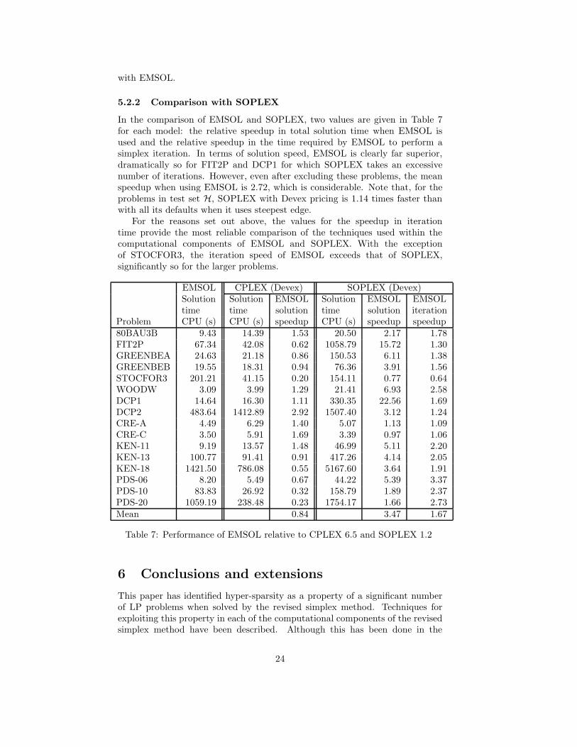
The results of the comparisons of EMSOL with CPLEX and SOPLEX, whenrun in the modes discussed above, are given in Table 7. Values of speedup whichare greater than unity indicate that EMSOL is faster.

5.2.1 Comparison with CPLEX

Table 7 shows that for the H problems EMSOL is faster on seven and CPLEXis faster on nine. On average, CPLEX is slightly faster: the mean speedup forEMSOL is 0.84. There is no consistent reason for the difference, with neithercode dominating the other in time per iteration or number of iterations. Becausethe different solvers do not follow the same paths to the solution, it is difficultto make precise comparisons. Also we have noticed that making an arbitraryperturbation to the pivot choice can double or half the solution time (thoughthe result presented in this paper are all for the EMSOL default settings). Thisdifference is due both to the variation in number of iterations taken and tovariation in the average amount of hyper-sparsity encountered on the solutionpath.

Brief comments by Bixby [3] and by Bixby et al [4] indicate that methodsto exploit hyper-sparsity in FTRAN, BTRAN and PRICE have been developedindependently for use in CPLEX [15]. These techniques, for which no detailshave been published, were introduced to CPLEX between versions 6 and 6.5.There may be other unpublished features of CPLEX unconnected with hyper-sparsity which contribute the the differences in performance when compared

23

with EMSOL.

5.2.2 Comparison with SOPLEX

In the comparison of EMSOL and SOPLEX, two values are given in Table 7for each model: the relative speedup in total solution time when EMSOL isused and the relative speedup in the time required by EMSOL to perform asimplex iteration. In terms of solution speed, EMSOL is clearly far superior,dramatically so for FIT2P and DCP1 for which SOPLEX takes an excessivenumber of iterations. However, even after excluding these problems, the meanspeedup when using EMSOL is 2.72, which is considerable. Note that, for theproblems in test set H, SOPLEX with Devex pricing is 1.14 times faster thanwith all its defaults when it uses steepest edge.

For the reasons set out above, the values for the speedup in iterationtime provide the most reliable comparison of the techniques used within thecomputational components of EMSOL and SOPLEX. With the exceptionof STOCFOR3, the iteration speed of EMSOL exceeds that of SOPLEX,significantly so for the larger problems.

EMSOL CPLEX (Devex) SOPLEX (Devex)Solution Solution EMSOL Solution EMSOL EMSOLtime time solution time solution iteration

Problem CPU (s) CPU (s) speedup CPU (s) speedup speedup80BAU3B 9.43 14.39 1.53 20.50 2.17 1.78FIT2P 67.34 42.08 0.62 1058.79 15.72 1.30GREENBEA 24.63 21.18 0.86 150.53 6.11 1.38GREENBEB 19.55 18.31 0.94 76.36 3.91 1.56STOCFOR3 201.21 41.15 0.20 154.11 0.77 0.64WOODW 3.09 3.99 1.29 21.41 6.93 2.58DCP1 14.64 16.30 1.11 330.35 22.56 1.69DCP2 483.64 1412.89 2.92 1507.40 3.12 1.24CRE-A 4.49 6.29 1.40 5.07 1.13 1.09CRE-C 3.50 5.91 1.69 3.39 0.97 1.06KEN-11 9.19 13.57 1.48 46.99 5.11 2.20KEN-13 100.77 91.41 0.91 417.26 4.14 2.05KEN-18 1421.50 786.08 0.55 5167.60 3.64 1.91PDS-06 8.20 5.49 0.67 44.22 5.39 3.37PDS-10 83.83 26.92 0.32 158.79 1.89 2.37PDS-20 1059.19 238.48 0.23 1754.17 1.66 2.73Mean 0.84 3.47 1.67

Table 7: Performance of EMSOL relative to CPLEX 6.5 and SOPLEX 1.2

6 Conclusions and extensions

This paper has identified hyper-sparsity as a property of a significant numberof LP problems when solved by the revised simplex method. Techniques forexploiting this property in each of the computational components of the revisedsimplex method have been described. Although this has been done in the

24

context of the primal simplex method, the techniques developed in this papercan be applied immediately to the dual simplex method since it has comparablecomputational components.

For the subset of our test problems that do not exhibit hyper-sparsity (H),the geometric mean speedup is 1.45, and for those problems which do exhibithyper-sparsity (H′), the speedup is substantial, increases with problem size andhas a mean value of 5.38.

For this latter subset of problems our implementation of the revised simplexwhich exploits hyper-sparsity has been shown to be comparable to the leadingcommercial simplex solver and several times faster than the leading public-domain solver. Although this performance gain is substantial for only a subsetof LP problems, the amenable problems in this paper are of genuine practicalvalue and the techniques yield some performance improvement in all but one ofthe test problems.

The authors would like to thank John Reid who brought the Gilbert-Peierlsalgorithm to their attention and made valuable comments on an earlier versionof this paper.

References

[1] R. H. Bartels. A stabilization of the simplex method. Numer. Math.,16:414–434, 1971.

[2] J. Bisschop and A. J. Meeraus. Matrix augmentation and partitioning inthe updating of the basis inverse. Mathematical Programming, 13:241–254,1977.

[3] R. E. Bixby. Solving real-world linear programs: A decade and more ofprogress. Operations Research, 50(1):3–15, 2002.

[4] R. E. Bixby, M. Fenelon, Z. Gu, E. Rothberg, and R. Wunderling.MIP: Theory and practice closing the gap. In M. J. D. Powell andS. Scholtes, editors, System Modelling and Optimization: Methods, Theoryand Applications, pages 19–49. Kluwer, The Netherlands, 2000.

[5] W. J. Carolan, J. E. Hill, J. L. Kennington, S. Niemi, and S. J. Wichmann.An empirical evaluation of the KORBX algorithms for military airliftapplications. Operations Research, 38(2):240–248, 1990.

[6] V. Chvatal. Linear Programming. Freeman, 1983.

[7] G. B. Dantzig and W. Orchard-Hays. The product form for the inverse inthe simplex method. Math. Comp., 8:64–67, 1954.

[8] J. J. Forrest and D. Goldfarb. Steepset-edge simplex algorithms for linearprogramming. Mathematical Programming, 57:341–374, 1992.

[9] J. J. H. Forrest and J. A. Tomlin. Updated triangular factors of the basisto maintain sparsity in the product form simplex method. MathematicalProgramming, 2:263–278, 1972.

25

[10] D. M. Gay. Electronic mail distribution of linear programming testproblems. Mathematical Programming Society COAL Newsletter, 13:10–12, 1985.

[11] J. R. Gilbert and T. Peierls. Sparse partial pivoting in time proportionalto arithmetic operations. SIAM J. Sci. Stat. Comput., 9(5):862–874, 1988.

[12] J. A. J. Hall and K. I. M. McKinnon. Hyper-sparsity in the revised simplexmethod and how to exploit it. Technical Report MS00-015, Department ofMathematics and Statistics, University of Edinburgh, 2000. Submitted toSIAM Journal of Optimization.

[13] J. A. J. Hall and K. I. M. McKinnon. LP test problems.http://www.maths.ed.ac.uk/hall/PublicLP/, 2002.

[14] P. M. J. Harris. Pivot selection methods of the Devex LP code.Mathematical Programming, 5:1–28, 1973.

[15] ILOG. CPLEX 6.5 Reference Manual, 1999.

[16] R. D. McBride and J. W. Mamer. Solving multicommodity flow problemswith a primal embedded network simplex algorithm. INFORMS Journalon Computing, 9(2):154–163, Spring 1997.

[17] R. D. McBride and J. W. Mamer. A decomposition-based pricingprocedure for large-scale linear programs: an application to the linearmulticommodity flow problem. INFORMS Journal on Computing,46(5):693–709, May 2000.

[18] H. D. Mittelmann. Benchmarks for optimization software.http://www.plato.la.asu.edu/bench.html, April 2002.

[19] J. A. Tomlin. Pivoting for size and sparsity in linear programming inversionroutines. J. Inst. Maths. Applics, 10:289–295, 1972.

[20] R. Wunderling. Paralleler und objektorientierter simplex. Technical ReportTR-96-09, Konrad-Zuse-Zentrum fur Informationstechnik Berlin, 1996.

[21] R. Wunderling, A. Bley, T. Pfender, and T. Koch. SOPLEX 1.2.0, 2002.

26