hyper-parameter learning for graph …zhangx/papers/zhangmsc06.pdfhyper-parameter learning for graph...
TRANSCRIPT

HYPER-PARAMETER LEARNING FOR GRAPH
BASED SEMI-SUPERVISED LEARNING ALGORITHMS
ZHANG XINHUA
(B. Eng., Shanghai Jiao Tong University, China)
A THESIS SUBMITTED
FOR THE DEGREE OF MASTER OF SCIENCE
DEPARTMENT OF COMPUTER SCIENCE
NATIONAL UNIVERSITY OF SINGAPORE
2006

i
Acknowledgements
First of all, I wish to express my heartfelt gratitude to my supervisor Prof. Lee Wee Sun who guided me into the research of machine learning. When I first walked into his office, I had only limited knowledge about the ad hoc early-time learning algo-rithms. He introduced me to the state-of-the-art in the current machine learning community, such as graphical models, maximum entropy models and maximum margin models. He is always patient and open to hear my (immature) ideas, obsta-cles, and then pose corrections, suggestions and/or solutions. He is full of wonder-ful ideas and energetic with many emails off office hour and even at small hours. I am always impressed by his mathematical rigor, sharp thinking and insight. He gave me a lot of freedom and sustained encouragement to pursue my curiosity, not only in the materials presented in this thesis, but also much other work before it. I would also like to thank my Graduate Research Paper examiners Prof. Rudy Setiono and Prof. Ng Hwee Tou, who asked pithy questions during my presentation, commented on the work and advised on further study. I also want to express my thanks to Prof. Ng for generously letting me use the Matlab Compiler on his Linux server twinkle. This tool significantly boosted the efficiency of implementation and experiments. Moreover, the graph reading group co-organized by Prof. Lee Wee Sun, Dr. Teh Yee Whye, Prof. Ng Hwee Tou, and Prof. Kan Min Yen has been very enriching for broadening and deepening my knowledge in graphical models. These biweekly discussions bring together faculty and students with shared interest, and offer an op-portunity to clarify puzzles and exchange ideas. Last (almost) but not least, I wish to thank my fellow students and friends, the col-laboration with whom made my Master’s study life a very memorable experience. Mr. Chieu Hai Leong helped clarify the natural language processing concepts espe-cially on named entity recognition. He also helped me warm-heartedly with a lot of practical problems such as implementation, the usage of computing clusters and MPI. The discussions with Dr. Dell Zhang on graph regularization are also enlightening. Finally, I owe great gratitude to the School of Computing and Singapore-MIT Alli-ance which provided latest software, high-performance computing clusters and tech-nical support for research purposes. Without these facilities, the experiments would have been prolonged to a few months.

ii
Table of Contents
Summary.......................................................................................................................v
List of Tables................................................................................................................vi
List of Figures.............................................................................................................vii
Chapter 1 Introduction and Literature Review .....................................................1
1.1 Motivation and definition of semi-supervised learning in machine learning............. 1
1.1.1 Different learning scenarios: classified by availability of data and label ........... 3
1.1.2 Learning tasks benefiting from semi-supervised learning.................................. 8
1.2 Why do unlabelled data help: an intuitive insight first ............................................ 10
1.3 Generative models for semi-supervised learning .................................................... 12
1.4 Discriminative models for semi-supervised learning .............................................. 15
1.5 Graph based semi-supervised learning.................................................................... 22
1.5.1 Graph based semi-supervised learning algorithms........................................... 23
1.5.1.1 Smooth labelling.......................................................................................... 23
1.5.1.2 Regularization and kernels........................................................................... 27
1.5.1.3 Spectral clustering ....................................................................................... 29
1.5.1.4 Manifold embedding and dimensionality reduction..................................... 32
1.5.2 Graph construction .......................................................................................... 34
1.6 Wrapping algorithms............................................................................................... 36
1.7 Optimization and inference techniques ................................................................... 41
1.8 Theoretical value of unlabelled data ....................................................................... 43
Chapter 2 Basic Framework and Interpretation .................................................45
2.1 Preliminaries, notations and assumptions................................................................ 45
2.2 Motivation and formulation .................................................................................... 46
2.3 Interpreting HEM 1: Markov random walk............................................................. 49
2.4 Interpreting HEM 2: Electric circuit ....................................................................... 51
2.5 Interpreting HEM 3: Harmonic mean ..................................................................... 53
2.6 Interpreting HEM 4: Graph kernels and heat/diffusion kernels............................... 55
2.6.1 Preliminaries of graph Laplacian..................................................................... 55

iii
2.6.2 Graph and kernel interpretation 1: discrete time soft label summation............ 58
2.6.3 Graph and kernel interpretation 2: continuous time soft label integral ............ 60
2.7 Interpreting HEM 5: Laplacian equation with Dirichlet Green’s functions ............. 61
2.8 Applying matrix inversion lemma........................................................................... 61
2.8.1 Active learning ................................................................................................ 62
2.8.2 Inductive learning............................................................................................ 64
2.8.3 Online learning................................................................................................ 64
2.8.4 Leave-one-out cross validation........................................................................ 65
2.8.5 Two serious cautions ....................................................................................... 66
Chapter 3 Graph Hyperparameter Learning.......................................................68
3.1 Review of existing graph learning algorithms......................................................... 68
3.1.1 Bayes network through evidence maximization .............................................. 69
3.1.2 Entropy minimization...................................................................................... 72
3.2 Leave-one-out hyperparameter learning: motivation and formulation .................... 74
3.3 An efficient implementation ................................................................................... 81
3.4 A mathematical clarification of the algorithm......................................................... 87
3.5 Utilizing parallel processing ................................................................................... 91
Chapter 4 Regularization in Learning Graphs ....................................................93
4.1 Motivation of regularization ................................................................................... 93
4.2 How to regularize? A brief survey of related literature ........................................ 96
4.2.1 Regularization from a kernel view................................................................... 96
4.2.2 Regularization from a spectral clustering view................................................ 98
4.3 Graph learning regularizer 1: approximate eigengap maximization...................... 100
4.4 Graph learning regularizer 2: first-hit time minimization...................................... 102
4.4.1 Theoretical proof and condition of convergence............................................ 104
4.4.2 Efficient computation of function value and gradient.................................... 108
4.5 Graph learning regularizer 3: row entropy maximization...................................... 109
4.6 Graph learning regularizer 4: electric circuit conductance maximization ............. 110
Chapter 5 Experiments......................................................................................... 112

iv
5.1 Algorithms compared............................................................................................ 112
5.2 Datasets chosen..................................................................................................... 116
5.3 Detailed procedure of cross validation with transductive learning ........................ 118
5.4 Experimental results: comparison and analysis..................................................... 121
5.4.1 Comparing LOOHL+Sqr with HEM and MinEnt, under threshold and CMN122
5.4.1.1 Comparison on original forms ................................................................... 122
5.4.1.2 Comparison on probe forms....................................................................... 126
5.4.2 Comparing four regularizers of LOOHL, under threshold and CMN ............ 129
Chapter 6 Conclusions and Future Work ...........................................................135
Bibliography .............................................................................................................139
Appendix A Dataset Description and Pre-processing........................................147
A.1. Handwritten digits discrimination: 4 vs 9 ............................................................. 147
A.2. Cancer vs normal .................................................................................................. 151
A.3. Reuters text categorization: "corporate acquisitions" or not.................................. 154
A.4. Compounds binding to Thrombin ......................................................................... 156
A.5. Ionosphere ............................................................................................................ 159
Appendix B Details of Experiment Settings .......................................................160
B.1. Toolboxes used for learning algorithm implementation ........................................ 160
B.2. Dataset size choice................................................................................................ 161
B.3. Cross validation complexity analysis .................................................................... 162
B.4. Miscellaneous settings for experiments................................................................. 163
Appendix C Detailed Result of Regularizers......................................................171

v
Summary
Over the past few years, semi-supervised learning has gained considerable interest
and success in both theory and practice. Traditional supervised machine learning
algorithms can only make use of labelled data, and reasonable performance is often
achieved only when there is a large number of labelled data, which can be expensive,
labour and time consuming to collect. However, unlabelled data is usually cheaper
and easier to obtain, though it lacks the most important information: label. The
strength of semi-supervised learning algorithms lies in its ability to utilize a large
quantity of unlabelled data to effectively and efficiently improve learning.
Recently, graph based semi-supervised learning algorithms are being intensively
studied, thanks to its convenient local representation, connection with other models
like kernel machines, and applications in various tasks like classification, clustering
and dimensionality reduction, which naturally incorporates the advantages of unsu-
pervised learning into supervised learning.
Despite the abundance of graph based semi-supervised learning algorithms, the fun-
damental problem of graph construction, which significantly influences performance,
is underdeveloped. In this thesis, we tackle this problem under the task of classifi-
cation by learning the hyperparameters of a fixed parametric similarity measure,
based on the commonly used low leave-one-out error criterion. The main contribu-
tion includes an efficient algorithm which significantly reduces the computational
complexity, a problem that plagues most leave-one-out style algorithms. We also
propose several novel approaches for graph learning regularization, which is so far a
less explored field as well. Experimental results show that our graph learning algo-
rithms improve classification accuracy compared with graphs selected by cross vali-
dation, and also beat the preliminary graph learning algorithms in literature.

vi
List of Tables
Table 2.1 Relationship of eigen-system for graph matrices......................................56
Table 3.1 Computational cost for term 1 ..................................................................85
Table 3.2 Computational cost for term 2 ..................................................................86
Table 5.1 Comparison of semi-supervised learning algorithms' complexity..........115
Table 5.2 Summary of the five datasets’ property ..................................................117
Table 5.3 Self-partitioning diagram for transductive performance evaluation .......120
Table 5.4 Pseudo-code for k-fold semi-supervised cross validation.......................121
Table A.1 Cancer dataset summary.........................................................................152
Table A.2 Compound binding dataset summary .....................................................159
Table B.1 Hardware and software configurations of computing cluster ................170

vii
List of Figures
Figure 1.1 Illustration of st-mincut algorithm...........................................................24
Figure 2.1 Electric network interpretation of HEM..................................................52
Figure 2.2 Static induction model for semi-supervised learning ..............................54
Figure 2.3 Relationship between graph Laplacian, kernel, and covariance matrix ..67
Figure 3.1 Bayes network of hyperparameter learning.............................................69
Figure 3.2 Output transformation functions for leave-one-out loss..........................77
Figure 3.3 Pseudo-code for the framework of the efficient implementation ............88
Figure 4.1 Examples of degenerative leave-one-out hyperparameter labelling .......93
Figure 4.2 Eigenvalue distribution example of two images .....................................99
Figure 4.3 Example of penalty function over eigenvalues .....................................101
Figure 4.4 Circuit regularizer..................................................................................110
Figure 5.1 Accuracy of LOOHL+Sqr, HEM and MinEnt on 4vs9 (original)......123
Figure 5.2 Accuracy of LOOHL+Sqr, ....................................................................123
Figure 5.3 Accuracy of LOOHL+Sqr, HEM and MinEnt on text (original) ..........123
Figure 5.4 Accuracy of LOOHL+Sqr, ....................................................................123
Figure 5.5 Accuracy of LOOHL+Sqr, HEM and MinEnt on ionosphere...............124
Figure 5.6 Accuracy of LOOHL+Sqr, HEM and MinEnt on 4vs9 (probe) ............127
Figure 5.7 Accuracy of LOOHL+Sqr, ....................................................................127
Figure 5.8 Accuracy of LOOHL+Sqr, HEM and MinEnt on text (probe)..............127
Figure 5.9 Accuracy of LOOHL+Sqr, ....................................................................127
Figure 5.10 Accuracy of four regularizers on 4vs9 (original) ................................132
Figure 5.11 Accuracy of four regularizers on cancer (original) .............................132
Figure 5.12 Accuracy of four regularizers on text (original)..................................132
Figure 5.13 Accuracy of four regularizers on thrombin (original) .........................133
Figure 5.14 Accuracy of four regularizers on ionosphere ......................................133
Figure 5.15 Accuracy of four regularizers on 4vs9 (probe)....................................133

viii
Figure 5.16 Accuracy of four regularizers on cancer (probe).................................134
Figure 5.17 Accuracy of four regularizers on text (probe) .....................................134
Figure A.1 Image examples of handwritten digit recognition ................................148
Figure A.2 Probe feature sampling example for handwritten digit recognition .....150
Figure A.3 Comparison of the real data and the random probe data distributions .155
Figure C.1 Accuracy of four regularizers on 4vs9 (original) under rmax ................172
Figure C.2 Accuracy of four regularizers on 4vs9 (original) under rmedium ............172
Figure C.3 Accuracy of four regularizers on 4vs9 (original) under rmin .................172
Figure C.4 Accuracy of four regularizers on 4vs9 (probe) under rmax....................173
Figure C.5 Accuracy of four regularizers on 4vs9 (probe) under rmedium................173
Figure C.6 Accuracy of four regularizers on 4vs9 (probe) under rmin ....................173
Figure C.7 Accuracy of four regularizers on cancer (original) under rmax..............174
Figure C.8 Accuracy of four regularizers on cancer (original) under rmedium..........174
Figure C.9 Accuracy of four regularizers on cancer (original) under rmin ..............174
Figure C.10 Accuracy of four regularizers on cancer (probe) under rmax ...............175
Figure C.11 Accuracy of four regularizers on cancer (probe) under rmedium ...........175
Figure C.12 Accuracy of four regularizers on cancer (probe) under rmin ...............175
Figure C.13 Accuracy of four regularizers on text (original) under rmax ................176
Figure C.14 Accuracy of four regularizers on text (original) under rmedium ............176
Figure C.15 Accuracy of four regularizers on text (original) under rmin ................176
Figure C.16 Accuracy of four regularizers on text (probe) under rmax ...................177
Figure C.17 Accuracy of four regularizers on text (probe) under rmedium ...............177
Figure C.18 Accuracy of four regularizers on text (probe) under rmin....................177
Figure C.19 Accuracy of regularizers on thrombin (original) under rmax ...............178
Figure C.20 Accuracy of regularizers on thrombin (original) under rmedium ...........178
Figure C.21 Accuracy of regularizers on thrombin (original) under rmin ...............178
Figure C.22 Accuracy of four regularizers on ionosphere under rmax.....................179
Figure C.23 Accuracy of four regularizers on ionosphere under rmedium.................179
Figure C.24 Accuracy of four regularizers on ionosphere under rmin .....................179

1
Chapter 1 Introduction and Literature Review
In this chapter, we review some literature on semi-supervised learning. As an introduction,
we first take a look at the general picture of machine learning, in order to see the position,
role and motivation of semi-supervised learning in the whole spectrum. Then we focus on
various algorithms in semi-supervised learning. There is a good review on this topic in
(Zhu, 2005). However, we will incorporate some more recently published work, use our
own interpretation and organization, and tailor the presentation catering for our original
work in this thesis. Careful consideration is paid to the breadth/completeness of the survey
and the relevance to our own work.
1.1 Motivation and definition of semi-supervised learning in machine learning
The first question to ask is what is semi-supervised learning and why do we study it. To
answer this question, it is useful to take a brief look at the big picture of machine learning
and to understand the unsolved challenges. We do not plan to give any rigorous definition
of most terminologies (if such definition exists). Instead, we will use a running example,
news web page interest learning, to illustrate the different facets of machine learning, in-
cluding tasks, styles, form and availability of data and label.
Suppose there is a news agency which publishes their news online. The subscribers can log
onto their own accounts (not free unfortunately) and read the news they are interested in.
On each web page, there are 10 pieces of news, each with a title, a short abstract and a link

2
to the full text. Once the reader gets interested in a certain piece of news after reading the
abstract, he/she will click into the full story. So the web site can know whether the reader
is interested in a piece of news by measuring the clicks. So by “news”, we only refer to the
abstract in the form of plain text for simplicity.
To promote subscription, the news agency would like to find out the interest of the readers
in order to streamline the collection, and composition of the news pool to satisfy common
interests. Knowing the readers’ interest will also allow the agency to present the news ca-
tering for each individual’s preference, e.g., in what order should the news be presented,
whether some links to background information or related news need to be inserted and what
they are. Unfortunately, it is normally not advisable to ask readers to fill up a questionnaire.
Firstly, most readers feel it far easier to say whether a specific piece of news is interesting,
than to generalize and precisely describe their interest. Secondly, readers’ interest may
change from time to time and it is impossible to ask readers to update the personal interest
information regularly, because besides inconvenience, the change may be too subtle to be
noticed by readers themselves. Thirdly, the less we ask our subscribers to do, the better.
Thus, it is highly desirable to automatically learn the interest of the readers from their past
read news. As the simplest case adopted in the following section 1.1.1, we only care about
the crisp classification: interested or not. To motivate the use of semi-supervised learning,
we first study a variety of different scenarios of learning, according to the availability of data
(text) and label (interest).

3
1.1.1 Different learning scenarios: classified by availability of data and label
In this section we divide the learning scenarios based on the availability of data and label in dif-
ferent phases of experiment and the different querying/sampling mechanism.
1. Supervised learning
When a subscriber first logs onto the web site, the best we can do is just to list some com-
monly interesting news. Then we record which news articles attracted the reader and
which do not. Finally we obtain a set of tuples <xi, yi>, where xi stands for the news i (pre-
cisely, title and abstract) and yi stands for interested in xi or not. Then we learn a function
which can predict whether the reader will be interested in an unseen piece of news x. At
the second time the user logs on, the system can organize the news catering for the user’s
interest learned from the first time. Note the function can be in any form: rule based,
real-valued function with a threshold like a neural network, or a segment of program learned
by genetic algorithm, etc., as long as it is computable.
2. Unsupervised learning
In this setting, the readers are not involved. We can imagine it as an offline process on the
new agency’s web server. The goal is to learn an inner structure of the news articles,
which includes clustering similar articles into groups, reducing the dimensionality of the
news pool by mapping news into a smaller set of synopsis on certain facets such as: who,
when, where, category (sports/entertainment/politics), length, etc. In theory, these facets
(or more rigorously called dimensions in lower dimensional spaces), are not necessarily ex-

4
plicitly defined and their distance on a learned manifold is of more interest.
3. Semi-supervised learning
So far so good, at least in task specification. However, in supervised learning, it is usually
necessary have a large set of labelled data before reasonable prediction accuracy can be
achieved. For example, in the UseNet news experiment, (Lang, 1995) found that after a
person read and hand-labelled about 1000 articles, a learned classifier achieved precision of
about 50% when making predictions for only the top 10% of documents about which it was
most confident. Obviously, no reader or news agency will accept such a low learning rate.
A dozen articles may be the upper limit that they can tolerate. Other examples include1:
Ø Satellite surveillance. In geographical information systems (GIS), remote imaging
and sensing are widely used to detect various natural structures and objects. However,
manually identifying objects in an image costs huge amount of time and effort, because
it usually involves field trip on a regular basis. On the other hand, modern sensors can
easily obtain a huge amount of unlabelled signals.
Ø Word sense disambiguation. It is labour consuming to determine the meaning of a
word in a given context. (Mihalcea & Chklovski, 2003) estimated that 80 person-year
is need to create manually labelled training data for about 20,000 words in a common
English dictionary. But documents and sentences are readily available in large amount.
Ø Predicting compounds’ ability to bind to a target site on a receptor for drug discovery.
It usually costs considerable expert human resources and financial expense to test the
1 Note for some cases, the labelling is easy but the data is complex to describe. See direc-tion 1 in Section 1.1.2.

5
binding activity. But the compound database is established and accessible.
Ø Handwritten character or speech recognition. With computers being more and
more user friendly, new input devices such as speech input and handwritten input are
becoming popular. However, it is extremely time consuming to annotate the speech
utterance at either phonetic level or word level. For some languages like Chinese
which is not based on a small alphabet and spelling, the task of labelling characters is
complicated.
On the other hand, in all of these cases (and many other cases) data without labels is usually
readily and cheaply available in large quantity. Therefore incorporating these unlabelled
data to learn a classifier will be very desirable if it does improve the performance. The
following two settings 3.1 and 3.2 are two concrete scenarios.
3.1. Transductive learning
This setting is the same as supervised learning, except that the pool of today’s news which
has not been displayed to the reader is also incorporated in the process of learning the classi-
fier. However the important feature of transductive learning is that the testing examples, or
the candidate set of news being evaluated of their appeal to the reader, are also known at the
learning phase. The learning process just labels the candidate news without outputting a
decision function, which was emphasized in the discussion of supervised learning in section
1.1.1. So when new unseen news is composed, the whole system must be learned again.

6
3.2. Inductive semi-supervised learning.
This is also similar to supervised learning. It is different from transductive learning in that
it does learn a function using labelled and unlabelled data, so it is easy to classify an unseen
example by just feeding it to the function. Normally this function does not change after
classifying the new unseen example.
4. Online learning
The crux of online learning is to update the classifier immediately after a testing example is
given, while its label can be given immediately or not. In our web news interest example,
when the reader chooses to view the next screen of 10 abstracts, the classifier will be
re-trained by making use of the reader’s interest in the news of the last screen. The updated
classifier will be used to choose another 10 articles for the next screen. The key factor here
is efficiency, because no reader will be willing to wait for long if such re-training will take
more than a few seconds. So most online learning algorithms are based on incremental
and/or local update (Kohonen, 2000). In contrast to online learning, offline learning means
that the classifier is learned on the server when the reader is logged off. Therefore the effi-
ciency may not be the bottleneck in offline learning.
5. Reinforcement learning
We consider an interesting situation, making one additional assumption that there is an iden-
tifiable group of subscribers who have the same interest pattern (called side information).
A reader of the group is a very busy CEO, and he only had time to skim the web pages,

7
reading the abstracts only and seldom clicks into a full text. So the web site cannot get any
response to its classification performance. However, after one month, the reader suddenly
decided to unsubscribe. Only at that moment can the system realize that it had been doing
an unsatisfactory job, and it can still learn from it to serve other subscribers in that group of
similar interest better. The most difficult challenge in reinforcement learning is to find a
good trade-off between exploitation: the reader did not unsubscribe so we just stick to the
current classifier; and exploration: why not try offering some news which is now regarded as
uninteresting by the imperfect classifier in case it would make the reader more satisfied and
recommend subscription for his friends or relatives, though at the risk of selecting even less
interesting news which finally results in unsubscription.
6. Active learning
This form of learning is very similar to reinforcement learning. Now suppose the user offers to,
or we are sure that the user is willing to, collaborate with the learner and answer whether he is
interested in an article selected by the learning system. Since this opportunity is rare and
valuable (say, when the reader just paid next month’s subscription fee), we should be very
careful in picking the most informative unlabelled articles, i.e., knowing the label of which
will most significantly improve the classifier. One early and popular approach is called
query-by-committee (QBC) (Freund et al., 1997; Seung et al., 1992), whereby an ensemble of
classifiers are built and the examples with the highest classification variance are selected.
(Freund et al., 1997) showed theoretically that if there is no error in labelling, QBC can ex-
ponentially reduce the number of labelled examples needed for learning. As for approaches

8
based on a single classifier instead of a committee, (Lewis & Gale, 1994; Lewis, 1995) ex-
amined pool-based uncertainty sampling and relevance sampling. (Schohn & Cohn, 2000)
used an approach for SVM, selecting the example that is closest to the linear decision bound-
ary given by the classifier. (Tong & Koller, 2001) used SVM as well, but did selection to
maximally reduce the size of the version space of good hypotheses.
1.1.2 Learning tasks benefiting from semi-supervised learning
With semi-supervised learning well motivated, we are interested in what kind of learning
tasks it can help. Can we benefit from unlabelled data in tasks other than classification?
The answer is yes. Almost all classical machine learning tasks have been shown to be able
to benefit from unlabelled data points, though hurting of performance is also frequently re-
ported. We mention a few tasks which are related to the thesis. As semi-supervised
learning stands between supervised and unsupervised learning, it is expected that unsuper-
vised learning techniques will also be helpful and are thus studied.
Ø Clustering and dimensionality reduction
We have discussed clustering and dimensionality reduction in section 1.1 under unsuper-
vised learning. We just want to emphasize that these tasks can also be carried out in a su-
pervised or semi-supervised setting, because it is usually beneficial to let the labels guide the
process (Grira et al., 2004).
Ø Regression

9
In this task, we are more ambitious and want to learn the extent to which the reader is inter-
ested. This can be any real number or bounded in [0, 1] up to definition. For example,
readers can spend a long time (normalized by word number) reading one article or can
manually score an article by 1 star to 5 stars.
Ø Ranking
Suppose that each screen can display at most 10 pieces of news. Then we want to pick out
the 10 articles which are of top interest to the reader. This task is different from classifica-
tion in that it only concerns the ranking, and performance is not measured on the non-top-10
news.
Up to now, we have been making a simplified assumption that the data is just a plain-text
article and the label is just a Boolean value. Extensions can be made in two directions re-
lating to this thesis:
1. Feature engineering. The article can contain photos, video and audio, etc. So how to
integrate the heterogeneous forms of the data into a well organized ensemble of useful
features is a problem. For example, in bioinformatics a gene can have: DNA, mRNA
and amino acid sequences, expression profile in microarray experiments, location in a
partially known genetic network, location in a protein-protein interaction network, gene
ontology classification, and so on (De Bie, 2005).
2. Structured, especially sequential data. One example of this second direction of exten-
sion is to look at the news in sequel, rather than in separation. There is often a series

10
of reports in newspapers, and the appeal of each article is dependent on the articles in
the previous issues and on what it promises to cover in the forthcoming issues.
In this thesis, we only focus on the simple data representation, assuming that each data point
is just a real vector with a Boolean label. Realizing the motivation of semi-supervised
learning, the first few natural questions to ask are whether it really helps, why it helps and
how it helps.
1.2 Why do unlabelled data help: an intuitive insight first
In this section, we just give some intuitive explanations of the questions, together with ex-
amples. Detailed algorithms will be reviewed from the next section. At first glance, it
might seem that nothing is to be gained from unlabelled data. After all, an unlabelled
document does not contain the most important piece of information its label. But think-
ing in another way may reveal the value of unlabelled data. In the field of information re-
trieval, it is well known that words in natural language occur in strong co-occurrence pat-
terns (van Rijsbergen, 1977). Some words are likely to occur together in one document,
others are not. For example, when asking search engine Google about all web pages con-
taining the words sugar and sauce, it returns 1,390,000 results. When asking for the docu-
ments with the words sugar and math, we get only 191,000 results, though math is a more
popular word on the web than sauce. Suppose we are interested in recognizing web pages
about cuisine. We are given just a few known cuisine and non-cuisine web pages, along with
a large number of web pages that are unlabelled. By looking at the labelled data only, we

11
determine that pages containing the word sugar tend to be about cuisine. If we use this fact
to estimate the class of many unlabelled web pages, we might find that the word sauce oc-
curs frequently in the unlabelled examples that are now believed to be about cuisine. This
co-occurrence of the words sugar and sauce over the large set of unlabelled training data can
provide useful information to construct a more accurate classifier that considers both sugar
and sauce as indicators of positive examples.
In this thesis, we show how unlabelled data can be used to improve classification accuracy,
especially when labelled data are scarce. Formally, unlabelled data only informs us of the
distribution of examples in input space. In the most general case, distributional knowledge
will not provide helpful information to supervised learning. Consider classifying uniformly
distributed instances based on conjunctions of literals. Here there is no relationship be-
tween the uniform instance distribution and the space of possible classification tasks, thus
unlabelled data obviously cannot help.
No matter how justified it is, the co-occurrence is just an assumption we make. We need to
introduce appropriate assumptions/biases into our learner about some dependence between
the instance distribution and the classification task. Even standard supervised learning with
labelled data must introduce bias in order to learn. In a well-known and often-proven result
in (Watanabe, 1969), the theorem of the Ugly Duckling shows that without bias all pairs of
training examples look equally similar, and generalization into classes is impossible. This
result was foreshadowed long ago by both William of Ockham's philosophy of radical

12
nominalism in the 1300's and by David Hume in the 1700's. Somewhat more recently,
(Zhang & Oles, 2000) formalized and proved that supervised learning with unlabelled ex-
amples must assume a dependence between the instance distribution and the classification
task. In this thesis, we will look at several assumptions of such dependence.
We now go on to the survey of semi-supervised learning algorithms, restricted to classifica-
tion. We adopt the normal criterion to divide them into generative and discriminative
model. In the section after these general reviews, we will focus on graph based
semi-supervised learning algorithms, extending the focus from classification to clustering,
which are the main topics of the thesis. After these high level algorithms are introduced,
we summarize and review the optimization and inference techniques used therein. On top
of general semi-supervised learning algorithms, wrapping algorithms will be surveyed and
finally we briefly mention some investigation into the theoretical value of unlabelled data.
1.3 Generative models for semi-supervised learning
Perhaps the first kind of semi-supervised learning models proposed in machine learning re-
search are the generative models. Generative learning models the probability of generating
a data example for each class. Given a data example, the posterior probability of its be-
longing to each class is then calculated using Bayes rule. Mathematically, it assumes
( ) ( ) ( ), |p x y p y p x y= and ( ) ( ) ( )|y
p x p y p x y= ∑ .
The main assumptions include two parts:
1. How many different discrete y values to take on, also called components, generators,

13
clusters, topics, or mixtures. Using too few components will fail to capture the under-
lying structure while too many clusters will cause overfitting.
2. The parametric form of p(x | y) (e.g., Gaussian distribution). One crucial requirement
on this choice is that the model p(x, y) (not p(x | y)) must be identifiable, i.e., for a fam-
ily of distributions pθ (x, y) parameterized by θ , ( ) ( )1 2
, ,p x y p x yθ θ= implies
1 2θ θ= up to a permutation of mixture components. Otherwise, one can contrive an
example ( )1
,p x yθ , ( )2
,p x yθ and some observations, where the total likelihood of
the observations is the same for ( )1
,p x yθ and ( )2
,p x yθ . However, there exists a
point x0 such that ( ) ( )1 10 0| |p y x p y xθ θ ′> and ( ) ( )
2 20 0| |p y x p y xθ θ ′< , i.e., contra-
dictory decisions are made. Mixture of Gaussian is identifiable, and mixture of Ber-
noulli or uniform is not identifiable (Corduneanu & Jaakkola, 2001; McCallum & Ni-
gam, 1998; Ratsaby & Venkatesh, 1995).
Then what to be estimated are the values of p(y), and the parameters of p(x | y) (e.g., mean,
covariance), typically estimated by maximizing likelihood: ( ),i ii
p x y∏ for supervised
learning, by using the expectation maximization algorithm (see section 1.7). The main
reason why generative models are attractive for semi-supervised learning and thus histori-
cally earlier used to this end is that it can naturally incorporate unlabelled data into the
model and evidence by:
( ) ( ) ( ) ( ) ( ) ( ), | |i i i i i i iyi labeled i unlabeled i labeled i unlabeled
p x y p x p x y p y p x y p y∈ ∈ ∈ ∈
⋅ = ⋅ ∑∏ ∏ ∏ ∏ .
If we model by p(y | x), then
( ) ( ) ( ) ( ) ( ) ( ), | |i i i i i i i iyi labeled i unlabeled i labeled i unlabeled
p x y p x p y x p x p x p y x∈ ∈ ∈ ∈
⋅ = ⋅ ∑∏ ∏ ∏ ∏
14
where ( )| iy
p y x∑ is trivially equal to 1, and the unlabelled data cannot be utilized
straightforwardly. (Miller & Uyar, 1996; Nigam et al., 1998; Baluja, 1999) started using
maximum likelihood of mixture models to combine labelled and unlabelled data for classi-
fication. (Ghahramani & Jordan, 1994) used EM to fill in missing feature values of exam-
ples when learning from incomplete data by assuming a mixture model. Generative mix-
ture models have also been used for unsupervised clustering, whose parameters have been
estimated with EM (Cheeseman et al., 1988; Cheeseman & Stutz, 1996; Hofmann & Puzicha,
1998).
When model assumptions are correct, the generative models can usually learn fast because
their assumptions are quite strong and thus the model is quite restrictive, especially with a
fixed parametric form p(x | y). Moreover, as desired, unlabelled data will guarantee the im-
provement of performance (Castelli & Cover, 1996; Ratsaby & Venkatesh, 1995; Castelli &
Cover, 1995). However, high benefit is usually at high risk. If the model assumption de-
viates from the reality, then it will not be able to learn to satisfactory performance and unla-
belled data may hurt accuracy. Putting it another way for generative models specifically,
the classification accuracy and model likelihood should be correlated in order to make unla-
belled data useful. The details of the undesired role of unlabelled data will be discussed in
section 1.8.
To make the assumptions more realistic, a number of methods have been proposed. (Jordan
& Jacobs, 1994) proposed hierarchical mixture-of-experts that are similar to mixture models,

15
and their parameters are also typically set with EM. (Nigam, 2001; Nigam et al., 1999)
proposed introducing hierarchical class relationship: sub-topics under one relatively broad
topic (i.e., using multiple multinomials), or inversely, super-topics to generalize similar top-
ics. The first comprehensive work of semi-supervised generative model for text classifica-
tion is (Nigam et al., 1999b; Nigam, 2001). For more examples, see (Miller & Uyar, 1996;
Shahshahani & Landgrebe, 1994).
Finally, as a historical note, though the idea of generative models has been introduced to the
machine learning community for semi-supervised learning for about 10 years, it is not new
in the statistics community. At least as early as 1968, it was suggested that labelled and
unlabelled data could be combined for building classifiers with likelihood maximization by
testing all possible class assignments (Hartley & Rao, 1968; Day, 1969). (Day, 1969) pre-
sented an iterative EM-like approach for parameters of a mixture of two Gaussian distribu-
tions with known covariances from unlabelled data alone. Similar iterative algorithms for
building maximum likelihood classifiers from labelled and unlabelled data are primarily
based on mixtures of normal distributions (McLachlan, 1975; Titterington, 1976).
1.4 Discriminative models for semi-supervised learning
Instead of learning p(x | y) and then calculating p(y | x) by Bayes rule as in generative models,
the discriminative models directly learn p(y | x). For a lot of real world problems, we can
not model the input distribution with sufficient accuracy or the number of parameters to es-
timate for generative model is too large compared with the training data at hand. Then a

16
practical approach is to build classifiers by directly calculating its probability of belonging
to each class, p(y | x). However, this makes it less straightforward to incorporate unlabelled
data, whose only informative contribution lies in p(x). (Seeger, 2000) pointed out that if
p(x) and p(y | x) do not share parameters (coupled), then p(x) will be left outside of the pa-
rameter estimation process, leading to unlabelled data being ignored.
Using this interpretation, different discriminative semi-supervised learning algorithms can
be divided according to their assumption over the relationship between p(x) and p(y | x), i.e.,
how they are coupled. As commonly used in literature especially for two class classifica-
tions, p(y | x) is modelled by a real-valued soft label f (x), e.g.,
( ) exp( ( ))1| ,1 exp( ( ))
f xp y x ff x
αα
=+
, ( ) 10 | ,1 exp( ( ))
p y x ff xα
=+
(α > 0), (1.1)
and the hard label of x (positive/negative) is determined by applying some decision rules to f
(e.g., sign function or thresholding). So now we look at p(x) and f (x). Besides some gen-
eral requirements on f (x) as in supervised learning, f (x) is assumed to satisfy some addi-
tional conditions in semi-supervised learning. We now use these various assumptions to
divide the wide range of discriminative models. Note that some assumptions are just re-
statement of some others, and we present these assumptions from as many different perspec-
tives as possible, because in practice, different expressions can result in different levels of
difficulty in model design or mathematical formulation.
1. f (x) yields a confidently correct hard label on labelled data
This first requirement is usually a problem of choosing the loss function, with typical

17
choices as L1, L2 loss , ε-insensitive loss (Smola & Schölkopf, 2003; Vapnik, 1999; Vapnik,
1998), or even incorporating a noise model, e.g., Gaussian noise, sigmoid noise (Zhu et al.,
2003b), flipping noise (Kapoor et al., 2005), etc. Generally speaking, this loss alone will
not make use of the unlabelled data.
2. f (x) yields a confident labelling of unlabelled data by entropy minimization
(Zhu et al., 2003a) proposed learning the hyperparameters by minimizing the average label
entropy of unlabelled data. Lower entropy means more confident labelling. In
(Grandvalet & Bengio, 2004), entropy minimization was introduced as a regularizer or prior.
Unfortunately, entropy minimization does not have unique solutions because for a single
random variable x, p( x = 1) → 1 and p( x = 0) → 1 will both have small entropy. This as-
sumption also implies that different classes overlap at a low level, which may not be realistic
in some cases. For example, in two heavily overlapping Gaussians, the separator goes ex-
actly across the most ambiguous region and the unlabelled data there should have high en-
tropy. This constitutes a counter example for most of the following assumptions. How-
ever, it can be easily learned by generative models like two mixing Gaussians.
3. Both labelled and unlabelled data should have a large distance from the decision
boundary of f (x) (maximum margin)
This criterion is very similar to the previous one as large distance from decision boundary
usually means confident labelling. A simplification of f (x) is as a linear function wTx+b
and its decision boundary is a hyperplane. Now this assumption means that the linear

18
separator should maximize the margin over both the labelled and unlabelled examples (and
of course place the labelled examples on the correct side). A transductive support vector
machine (TSVM) (Vapnik, 1998) is designed by using this philosophy. The contribution of
unlabelled data is to expel the separating hyperplane away from them. However, as in the
assumption 2, the solution to such a maximum margin separator is not unique, because an
unlabelled point can lie on two different sides of the hyperplane with the same distance.
Moreover, finding the optimal hyperplane is NP-hard, so one must fall back on approximate
algorithms. (Joachims, 1999) designed an iterative relaxation algorithm and demonstrated
the efficacy of this approach for several text classification tasks. (Bennett & Demiriz, 1998)
proposed a computationally easier variant of TSVM and found small improvements on some
datasets. Other works include (Chapelle & Zien, 2005; Fung & Mangasarian, 1999).
However, (Zhang & Oles, 2000) argues that TSVMs are asymptotically unlikely to be help-
ful for classification in general, both experimentally and theoretically (via Fisher’s informa-
tion matrices) because its assumption may be violated. (Seeger, 2000) also cast the similar
doubt.
4. f (x) should not change quickly in regions where p(x) is high
This idea has been widely used in supervised learning, if we deem a “quickly changing” f as
a “complex” one. Balancing hypothesis space generality with predictive power is one of
the central tasks in inductive learning. The difficulties that arise in seeking an appropriate
tradeoff go by a variety of names: overfitting, data snooping, memorization, bias/variance

19
tradeoff, etc. They lead to a number of known solution techniques or philosophies, includ-
ing regularization, minimum description length, model complexity penalization (e.g., BIC,
AIC), Ockham’s razor (e.g., decision tree), training with noise, ensemble methods (e.g.,
boosting), structural risk minimization (e.g., SVMs), cross validation, holdout validation, etc.
Unlabelled data can provide a more accurate sampling of the function.
The biggest challenge is how to define a proper measure of the function’s complexity, which
is the synonym of “change quickly”. To proceed, we should define the meaning of
“change” and “quickly”. In semi-supervised learning, there are at least three different defi-
nitions which lead to different models.
Firstly, the most natural definition is the norm of gradient f x∂ ∂ or its associated
( )| ,p y x f x∂ ∂ . One example is TSVM. Using the ( )| ,p y x f defined in (1.1),
( )| ,p y x f x∂ ∂ reaches its maximum (for both y = 1 and y = 0) when f is 0. So this as-
sumption pushes the final learned separator ( f = 0) to low density regions (hopefully the
space between the clusters of the two classes), which the unlabelled data helps to locate.
Secondly, the Laplace operator: 2 2 2
2 2 21 2 m
f f fx x x
∂ ∂ ∂+ + +
∂ ∂ ∂ . Strictly speaking, this is the same as
2f x∂ ∂ in continuous compact space. It is usually difficult to calculate exactly and (Belkin &
Nigam, 2004; Belkin et al., 2004b) tried to approximate it discretely using graph Laplacian. We
will review the details in the next section.

20
Thirdly, mutual information I (x : y) between x and y (now we use hard labels directly). No-
ticing that I (x : y) describes how homogeneous the soft labels are, (Szummer & Jaakkola,
2002) proposed information regularization, which minimizes, on multiple overlapping re-
gions, the product of p(x) and the mutual information I (x : y) normalized by variance. Fur-
thermore, after some additional development in (Corduneanu & Jaakkola, 2003),
(Corduneanu & Jaakkola, 2004) formulated regularization as rate of information, discourag-
ing quickly varying p(y | x) when p(x) is large. Then it uses a local propagation scheme to
minimize the regularized loss on labelled data.
More measure based regularization is available in (Bousquet et al., 2003), assuming known
p(x), though there are open problems in applying the results to high dimensional tasks.
5. Similar/closer examples should have similar f (x)
k nearest neighbour (kNN) is the clearest representative of this assumption. In this assump-
tion, the contribution of unlabelled data is to provide additional neighbouring information,
which helps to propagate the labels among unlabelled points. (Zhu et al., 2003b) used kNN
for induction on unseen data. Most graph based semi-supervised learning algorithms to be
discussed in the next section are also making this assumption explicitly or implicitly. One
extension is from direct neighbour to a path connecting two points. Combining with the
above assumption 4, one can make a so-called cluster assumption: two points are likely to
have the same class if there is a path connecting them passing through regions of high den-
sity only. (Szummer & Jaakkola, 2001) assumed that the influence of one example A on

21
another example B is proportional to the probability of walking from A to B in t-step Markov
random walk. However, the parameter t is crucial and requires special care to select.
6. Entropy maximization
This seems to be contradictory to assumption 2, but in fact the entropy here is of classifier
parameters. (Jaakkola et al., 1999) proposed a maximum entropy discrimination model
based on maximum margin. It maximizes the entropy distribution over classifier parame-
ters, with constraints that the distance between each labelled example and decision boundary
(margin) should be no less than a fixed value, or incurring soft penalty as in SVM. Inter-
estingly, unlabelled data are also covered by margin constraints in order to commit to a cer-
tain class during parameter estimation by entropy maximization. The contribution of unla-
belled data is to provide a more accurate distribution over the unknown class labels. Clas-
sification is then performed in a Bayesian manner, combining the expected value of the ex-
ample's class over the learned parameter distribution. As for optimization method, an itera-
tive relaxation algorithm is proposed that converges to local minima, as the problem is not
convex. The experimental results for predicting DNA splice points using unlabelled data is
encouraging.
7. f (x) has a small norm in associated reproducing kernel Hilbert space
Some algorithms assume that the hypothesis space is a reproducing kernel Hilbert space
(RKHS). They regularize the f by its norm in this RKHS. SVM and TSVM can both be
viewed as examples of this assumption (Schölkopf & Smola, 2001). The unlabelled data is

22
used to define a richer RKHS and to give a more accurate regularization. It can be associ-
ated with the graph Laplacian as discussed in the next section by matrix pseudo-inversion.
Finally, we point out that there are some work which combines the generative models and
discriminative models. See (Zhu & Lafferty, 2005) as an example.
1.5 Graph based semi-supervised learning
In this section, we review the graph based semi-supervised learning algorithms. These al-
gorithms start with building a graph whose nodes correspond to the labelled and unlabelled
examples, and whose edges (non-negatively weighted or unweighted) correspond to the
similarity between the examples. They are discriminative, transductive and nonparametric
in nature. Intuitively, graph based methods are motivated by learning globally based on
local similarity.
A starting point for this study is the question of what constitutes a good graph. (Li &
McCallum, 2004) argued that having a good distance metric is a key requirement for success
in semi-supervised learning. As the final performance is not defined directly on graphs, but
rather on higher level learning algorithms which utilize graphs, we postpone this question
until the graph based learners are reviewed, and we first assume that a proper graph has been
given.

23
1.5.1 Graph based semi-supervised learning algorithms
Graphs can be used in a number of ways going far beyond the scope of this thesis. We just
review a few of them related to the project, namely: smooth labelling, regularization and
kernels, spectral clustering, and manifold embedding for dimensionality reduction.
1.5.1.1 Smooth labelling
In this category of classification methods, the soft labels of the set of labelled examples (L)
are clamped (or pushed) to the given labels, i.e., noiseless or zero training error. The task
is to find a labelling of the set of unlabelled examples (U), which is smooth on the graph.
Formally, it minimizes
( )2
,ij i j
i jw y y−∑ ,
where yi = 1 if xi is labelled positive and yi = 0 if xi is labelled negative.
Different algorithms have been proposed based on different constraints on yi for i U∈ . If
we restrict 0, 1iy ∈ , then we arrive at the st-mincut algorithm (Blum & Chawla, 2001).
The intuition behind this algorithm is to output a classification corresponding to partitioning
the graph in a way which minimizes the number of similar pairs of examples that are given
different labels. The idea originated from computer vision (Yu et al., 2002; Boykov et al.,
1998; Greig et al., 1989). (Blum & Chawla, 2001) applied it to semi-supervised learning.
The formulation is illustrated in Figure 1.1.

24
Figure 1.1 Illustration of st-mincut algorithm
The three labelled examples are denoted with + and –. They are connected to the respec-
tive classification nodes (denoted by triangles) with bold lines. Other three nodes are
unlabelled and finally the left one is classified as + and right two nodes are classified as –.
v+ and v are artificial vertices called classification nodes. They are connected to all posi-
tive examples and negative examples respectively, with infinite weight represented by bold
lines. Now we determine a minimum (v+, v) cut for the graph, i.e., find set of edges with
minimum total weight whose removal disconnects v+ and v. The problem can be solved
using max-flow algorithm, in which v+ is the source, v is the sink and the edge weights are
treated as capacities (e.g.,(Cormen et al., 2001)). Removing the edges in the cut partitions
the graph into two sets of vertices which we call V+ and V, with v V+ +∈ , v V− −∈ . We
assign positive label to all unlabelled examples in V+ and negative label to all examples in V.
(Blum & Chawla, 2001) also showed several theoretical proofs for the equivalence between
st-mincut and leave-one-out error minimization under various 1NN or kNN settings.
(Kleinberg & Tardos, 1999) considered this idea in multi-way cuts setting.
+
v+ v–
+ A

25
But an obvious problem of st-mincut is that it may lead to degenerative cuts. Suppose A is
the only negative labelled example in Figure 1.1. Then the partition given by st-mincut
may be the dashed curve. Obviously this is not desired. The remedies in (Blum &
Chawla, 2001), such as carefully adjusting edge weights, do not work across all problems
they study. To fix this problem, these algorithms usually require a priori fraction of posi-
tive examples in the test set, which is hard to estimate in practice when the training sets are
small. (Blum et al., 2004) used the idea of bagging and perturbed the graph by adding
random noise to the edge weights. On multiple perturbed graphs, st-mincut is applied and
the labels are determined by a majority vote, yielding a soft st-mincut. Other algorithms
like TSVM and co-training also suffer from similar degeneracy.
A simple analysis reveals the cause of the problem. The sum of the edge weights on the
cut is related to the number of edges being cut, which in turn depends directly on the size of
the two cut sets. In particular, the number of edges being cut with |V+| vertices on one side
and |V| vertices on the other side can potentially be |V+| ⋅ |V|. The st-mincut objective is
inappropriate, since it does not account for the dependency on the cut size. A natural way
proposed by (Joachims, 2003) is to normalize by dividing the objective with |V+| ⋅ |V|:
( , )| | | |cut V VV V
+ −
+ −⋅. This problem is related to ratiocut (Hagen & Kahng, 1992) in the unsuper-
vised setting, whose solution is NP-hard (Shi & Malik, 2000). So (Hagen & Kahng, 1992)
proposed good approximations to the solution based on the spectrum of the graph.
The idea of approximation motivated the relaxation of binary constraints 0,1iy ∈ . The

26
first step of relaxation is to allow y to assume real-valued soft labels. Using the notation in
section 1.4, we replace y by f, though the f value on labelled data is still fixed to 1 or 0.
(Zhu et al., 2003a) proposed minimizing ( )2
,ij i j
i jw f f−∑ over the f value of the unlabelled
data in continuous space. The solution is actually a minimal norm interpolation and it turns
out to be unique which can be simply calculated by solving a linear equation. This model
constitutes the basic framework of this thesis. It has been applied to medical image seg-
mentation (Grady & Funka-Lea, 2004), colorization of gray-level images (Levin et al., 2004),
and word sense disambiguation (Niu et al., 2005).
(Joachims, 2003) goes one step further by making the soft labels of labelled data unfixed,
and proposed a similar spectral graph transducer (SGT), which optimizes:
( ) ( )T Tc f C f f fγ γ− − + ∆ , under the constraint that 1 0Tnf =
and Tf f n= . Here
i l lγ − + for positively labelled data, i l lγ − +− for negatively labelled data, where
l+ and l– stand for the number of positive and negative labelled examples respectively.
0iγ = for unlabelled data. ( )ij ij ijji j w wδ∆ = −∑ (graph Laplacian). In this way,
the soft labels f on labelled data will be no longer fixed to 1 or 0, and the global optimal so-
lution can be found by spectral methods efficiently.
As a final analysis of semi-supervised smooth graphical labelling, (Joachims, 2003) posed
three postulates for building a good transductive learner:
1. It achieves low training error;
2. The corresponding inductive learner is highly self-consistent (e.g., low leave-one-out

27
error);
3. Averages over examples (e.g., average margin, pos/neg ratio) should have the same ex-
pected value in the training and in the test set.
St-mincut does not satisfy the third criterion, and the later algorithms patched it up.
1.5.1.2 Regularization and kernels
All the above mentioned algorithms of smooth labelling can be viewed as based on regu-
larization: ( )2
,ij i j
i jw f f−∑ . Define a matrix Δ, with ( )ij ij ijj
i j w wδ∆ = −∑ , this regu-
larizer can be written as: Tf f∆ . Δ is usually called graph Laplacian. Since ijjw∑ can
be wildly different for different i, there have been various ways proposed to normalize Δ.
One most commonly used one is 1/ 2 1/ 2D D− −∆ = ∆ , where D is a diagonal matrix with
ii ijjD w= ∑ . Using these concepts, we can simply re-write all the smoothing algorithms
above and there are some other examples in literature. (Zhou et al., 2003) minimized
( )2 Ti ii L
f y f f∈
− + ∆∑ . (Belkin et al., 2004a) used the same objective function except
replacing ∆ by p∆ , where p is a natural number, which is essentially Tikhonov regulari-
zation (Tikhonov, 1963). Refer to the relationship of approximation between graph Lapla-
cian and Laplace operator in section 2.6.1.
The real power of graph in regularization stems primarily from the spectral transformation
on its associated graph Laplacian and the induced kernels. (Smola & Kondor, 2003;
Chapelle et al., 2002) motivated the use of the graph as a regularizer by spectral graph the-

28
ory (Chung, 1997). According to this theory, the eigenvectors of Δ correspond to the local
minima of the function Tf f∆ . For eigenvector iφ with eigenvalue iλ , i
Tif
f fφ
λ=
∆ = .
Since the eigenvectors constitute a basis of the vector space, for any soft label vector
i iif α φ= ∑ , Tf f∆ = 2
i iiα λ∑ . Therefore we wish to penalize more seriously those iα
associated with larger eigenvalues iλ . How serious the penalty is as a function of iα and
iλ has motivated many different spectral transformation functions, because a simplest way
to describe this penalty relationship is by mapping λi to r( λi ), where r(•) is a non-negative
monotonically increasing function (larger penalty for larger λi). So Tf f∆ = ( ) 2i ii
r λ α∑ .
Commonly used r ( λ ) include:
( ) 21r λ σ λ= + (regularized Laplacian), ( ) ( )2exp 2r λ σ λ= (diffusion kernel)
( ) ( ) pr aλ λ −= − ( 1p ≥ , p-step random walk), ( ) ( ) 1cos / 4r λ λπ −= (Inverse cosine).
The form Tf f∆ has naturally elicited the connection between ∆ and kernels, because the
norm of any function f in a reproducing kernel Hilbert space induced by kernel K is
1Tf K f− . Based on this analogy, (Smola & Kondor, 2003) established and proved the re-
lationship †K = ∆ , where † stands for pseudo-inverse. Therefore, we now only need to ap-
ply the reciprocal of the above r(•) on the spectrum of Δ in order to derive a kernel.
(Kondor & Lafferty, 2002) proposed diffusion kernels by effectively using
( ) ( )1 2exp 2r λ σ λ− = − . ( ) ( )1 tr aλ λ− = − and ( ) ( ) 11r λ λ σ −− = + were used in
(Szummer & Jaakkola, 2001) for t-step random walk and in (Zhu et al., 2003b) for Gaussian
process respectively.

29
This kernel view offers the leverage of applying the large volume of tools in kernel theory,
such as the representer theorem (Schölkopf & Smola, 2001) to facilitate optimization
(Belkin et al., 2005). Moreover, since the new kernel is ( )1 Ti i ii
r λ φ φ−∑ , this view has
also opened window to learning the kernel by maximizing the kernel alignment (Cristianini
et al., 2001) or low rank mapping to feature space (Kwok & Tsang, 2003), with respect to
those hyperparameters σ, a, t. However, though it is more restrictive than the overly free
semi-definite programming algorithms (Lanckriet et al., 2004) which only require positive
semi-definiteness, these methods are too restrictive given the fixed parametric form. Con-
sidering the monotonically decreasing property of spectral transformation for kernels, (Zhu
et al., 2004) proposed a tradeoff by maximizing alignment with empirical data from a family
of kernels Ti i ii
µ φ φ∑ , with nonparametric constraints that i jµ µ≥ if and only if i jλ λ≤ .
Recently, (Argyriou et al., 2005) learns a convex combination of an ensemble of kernels de-
rived from different graphs.
Finally, for completeness, there are also some kernel based algorithms for generative models.
As an extension of Fisher kernel (Jaakkola & Haussler, 1998), a marginalized kernel for
mixture of Gaussians ( , )k kµ Σ is proposed: 11
( , ) ( | ) ( | )q Tkk
K x y p k x p k y x y−=
= Σ∑ (Tsuda
et al., 2002). But in addition to common problem of generative models, this method requires
building a generative model: finding parameters kµ and kΣ using unsupervised learning.
1.5.1.3 Spectral clustering
Why is clustering related to classification in a semi-supervised setting? One ideal situation

30
when clustering helps is: the whole set of data points are well clustered, with each cluster
being represented by a labelled data point. Then we can simply label the rest data in that
cluster by the same label. Generally, we are not that lucky because the clustering process is
blind to the labels, and its policy may be significantly different from the labelling mecha-
nism. However, studying the clustering algorithms does help us learn a graph, because no
matter how the data points are labelled, it is desirable that data from different classes are
well clustered, i.e., there exists some view based on which the result of clustering tallies with
the labelling mechanism. So studies in this area can inform us what makes a good graph,
hopefully in the form of an objective function to be optimized, though it is not the original
task of clustering.
A most natural model for clustering is generative mixture models. However, its parametric
density model with simplified assumptions (such as Gaussian) and the local minima in
maximum evidence estimation poses a lot of inconvenience. A promising alternative fam-
ily of discriminative algorithms formulate objective functions which can be solved by spec-
tral analysis (top eigenvectors), similar to the role of eigensystem mentioned in section
1.5.1.2 on kernel and regularization. A representative algorithm is normalized cut (Shi &
Malik, 2000), which minimizes: ( ) ( )( )
( )( )
, ,,
, ,cut A B cut A B
Ncut A Bassoc A V assoc B V
+ , where V is the
whole node set, A and B are the two disjoint sets V is to be partitioned into, and
( ) ,, utu A t V
assoc A V w∈ ∈
= ∑ (the total weight of edges from nodes in A to all nodes in the
graph). The normalized cut is minimized in two steps: first find a soft cluster indicator
vector, which is the eigenvector with the second smallest eigenvalue (sometimes directly

31
called second smallest eigenvector). The underlying math tool is the Rayleigh quotient
(Golub & van Loan, 1996). Secondly, discretize the soft indicator vector to get a hard
clustering. To find k clusters, the process is applied recursively (Spielman & Teng, 1996).
(Ng et al., 2001a) mapped the original data points to a new space spanned by the k smallest
eigenvectors of the normalized graph Laplacian (well, we present in a slightly different but
equivalent way of the original paper). Then k-means or other traditional algorithms are
performed in the new space to derive the k-way clustering directly. However there is still
disagreement on exactly which eigenvectors to use and how to discretize, i.e., derive clusters
from eigenvectors (Weiss, 1999). For large spectral clustering problems, this family of
algorithms are too computationally expensive, so (Fowlkes et al., 2004) proposed Nystrőm
method, which extrapolates the complete clustering solution using only a small number of
examples.
The soft indicators (actually the second smallest eigenvector) in normalized cut tell how
well the graph is naturally clustered. If the elements of the vector are numerically well
grouped within each class and well separated between classes (e.g., many close to 1, many
close to –1 and few near 0), then the discretization step will confidently classify them into
two parts. Otherwise, if we assume that the clustering algorithm is well designed and reli-
able, then we can conclude that the graph itself is not well constructed, i.e., heavy overlap-
ping between classes and large variance within each class. (Ng et al., 2001a) used eigen-
gap by matrix perturbation theory (Stewart & Sun, 1990) to present some desired property of
a good graph for clustering. The central idea is: if a graph has k well clustered groups, then

32
the clustering result is more stable (i.e., the smallest k eigenvectors are more stable to small
perturbations to graph edge weights) when the difference between the kth and (k + 1)th small-
est eigenvalues of the normalized graph Laplacian is larger. See more details of eigengap
in section 4.2.2.
1.5.1.4 Manifold embedding and dimensionality reduction
These are essentially techniques for unsupervised learning. The central idea of manifold is
that classification functions are naturally defined only on the sub-manifold in question rather
than the total ambient space. So transforming the representation of data points into a rea-
sonable model of manifold is effectively performing feature selection, noise reduction, and
data compression. These will hopefully improve classification. As this process does not
depend on examples’ label, unlabelled data can be naturally utilized by refining the ap-
proximation of the manifold by the weighted discrete graph.
For example, handwritten digit 0 can be fairly accurately represented as an ellipse, which is
completely determined by the coordinates of its foci and the sum of distances from the foci
to any point. Thus the space of ellipses is a five-dimensional manifold. Although a real
handwritten 0 may require more parameters, the dimensionality is absolutely less than am-
bient representation space, which is the number of pixels. In text data, documents are
typically represented by long vectors whereas researchers are convinced by experiments that
its space is a manifold, with complicated intrinsic structure occupying only a tiny portion of
the original space. The main problem is how to choose a reasonable model of manifold, or

33
more concretely speaking, how to find a proper set of basis of the manifold space.
(Belkin & Nigam, 2004; Belkin et al., 2004b) used the Laplace-Beltrami operator
2 2ii
x∆ = ∂ ∂∑ , which is positive semidefinite self-adjoint on twice differentiable functions.
When M is a compact manifold, ∆ has a discrete spectrum and its eigen-functions pro-
vide an orthogonal basis for the Hilbert space 2 ( )L M . Suppose we are given n points
x1,…, xn m∈R and the first l < n points have labels 1, 1ic ∈ − . First construct an adja-
cency graph with n nearest and reverse nearest neighbours, with distance defined as standard
Euclidean distance in mR , or other distance like angle/cosine. Then define adjacency ma-
trix n nW × . wij = 1 if points xi and xj are close (in some sense). Otherwise, wij = 0. Com-
pute p eigenvectors corresponding to the smallest p eigenvalues for the graph Laplacian.
They are proved to unfold the data manifold to form meaningful clusters. Now constitute a
matrix p nE × by stacking the transposition of the p eigenvectors in rows and the column or-
der corresponds to the original index of xi. Denote the left p l× sub-matrix of p nE × as
EL and calculate 1( )T TL L La E E E c−=
. Finally, for xi (i > l) the rule for classification is: ci = 1
if 1
0pij jj
e a=
≥∑ and ci = –1 otherwise. In essence, this is similar to spectral clustering
and there are many variants of such a PCA-style data representation (Ng et al., 2001a; Weiss,
1999).
Other graph based dimensionality reduction algorithms include locally linear embedding
(LLE) (Roweis & Saul, 2000), Isomap (de Silva & Tenenbaum, 2003; Tenenbaum et al.,
2000), multidimensional scaling (MDS) (Cox & Cox, 2001), semidefinite embedding

34
(Weinberger et al., 2005; Weinberger et al., 2004; Weinberger & Saul, 2004), etc. (Ham et
al., 2004) shed the insight that the first three are all kernel PCA on specially constructed
Gram matrices.
The contribution to classification by dimensionality reduction or manifold embedding is
similar to the role of feature selection, helping to find a lower dimensional (simpler) struc-
ture in the data which is expected to be related to the class labels of the data. However, it is
likely that the manifold is uncorrelated with the labels and this unsupervised technique will
then hurt the classification performance. (Weinberger et al., 2004) gives an example.
1.5.2 Graph construction
It is interesting that the question of how to construct a good graph has not received intensive
attention, albeit its fundamental role in graph based semi-supervised learning algorithms.
In the applications considered here, the graphs are closest to real data and interfaces to the
learning algorithm as an intermediate form of representation. It is conjectured that this
problem is very domain specific and depends mainly on prior expert knowledge. Their
utility is supposed to depend, to some extent, on the algorithms that they will ultimately be
used for.
From an unsupervised view, the graph should represent the underlying manifolds well.
Intuitively, it should avoid shortcuts that travel outside a manifold, avoid gaps that errone-
ously disconnect regions of a manifold, and be dense within the manifold and clusters.

35
Also, even if the algorithms differ with respect to connectedness, (clustering wants the graph
to be disconnected, while for manifold learning the graph should be connected), they both
want at least the inside of the clusters, or dense areas of the manifold, to be enhanced rela-
tive to the between-cluster, or sparse manifold connections.
In (Zhu, 2005; Carreira-Perpiňán & Zemel, 2004) , the following graph construction ap-
proaches are summarized. Note the edge weights wij are all based on a given distance dij
between all node pairs (i, j), and wij should be a monotonically decreasing function of dij.
1. Fully connected graphs, which are often used for spectral clustering and multidimen-
sional scaling.
2. Fixed grid. Connect each point to some small fixed number of neighbours in a
pre-defined grid, generally used in image segmentation.
3. Unweighted kNN graph. Connect node i and j by an edge with weight 1, if node i is
one of node j’s k nearest neighbours or vice versa. The desirable property of this con-
struction is the spatial adaptive scaling, i.e., in low density regions the distance between
k nearest neighbours can be farther than in high density regions.
4. Unweighted ε-ball graph. Connect node i and j by an edge with weight 1, if dij ≤ ε.
5. tanh-weighted graph. Define 1 2(tanh( ( ) 1)) 1) / 2ij ijw dα α− − + . This function will
create a soft cutoff around length α2 and the hyperbolic tangent function simulates
ε-ball, with α1 and α2 controlling the slope and cutoff value respectively. It has a nota-
ble advantage that the graph is continuous with respect to dij, so gradient based learning
methods are applicable.

36
6. RBF weighted graph: ( )2 2expij ijw d σ− . σ controls the decay rate, and σ is
also called bandwidth. This graph is continuous with respect to dij.
The hyperparameters ε, k draw a considerable impact on the performance of graph algorithm.
And because they are at the lowest layer, the normal cross validation algorithms have to con-
struct graphs for a range of hyperparameter values, redo the graph based learning algorithm and
then pick the best settings. In order to circumvent these trouble, (Carreira-Perpiňán & Zemel,
2004) proposed building robust graphs by applying random perturbation and edge removal from
an ensemble of minimum spanning trees.
However, these methods still depend on a given distance dij. In real practice, rarely are we
simply given a correct distance metric. Even restricted to Euclidean distance, the square dis-
tance along feature s, t between xi and xj may be attached with different importance for the
learning task. In this thesis, we restrict our attention to Gaussian RBF weighted graphs:
( )( )2 2, ,expij i k j k kk
w x x σ− −∑ and learn different bandwidth σ k for different dimensions k.
All procedures apply to tanh-weighted graph with no change, except rewriting the gradient for-
mula.
1.6 Wrapping algorithms
Just as there are ensemble methods in supervised learning such as boosting and bagging
which can be generically applied on top of almost all algorithms to boost the performance,
so are there such counterparts in semi-supervised learning. We call them wrapping algo-

37
rithms. Here we briefly overview some well known wrappers: self-training, co-training,
co-boosting, co-validation, co-testing, and down-weighting.
1. Self-training
The earliest and simplest wrapping algorithm is self-training. Its basic idea is:
1. The initial labelled set L and unlabelled set U are the originally labelled and unla-
belled data, respectively.
2. Train the classifier by L, and classify the data in U.
3. Pick the most confidently classified examples and move them from U to L with the
predicted labels.
4. Go to step 2 and retrain until U is empty.
So the algorithm uses its own predictions to supervise itself, and one can expect that mis-
takes can be propagated and magnified through iteration. There are some unlearning or
anti-learning algorithms to early detect and stop the propagation of errors. Applications of
self-training are reported in (Yarowsky, 1995) for word sense disambiguation, (Riloff et al.,
2003) for subjective noun identification, (Maeireizo et al., 2004) for emotional and
non-emotional dialogue classification, and (Weiss, 1999) for object detection in images, etc.
2. Co-training
The idea of co-training is: suppose the feature of each data point is composed of two sets,
which are separately used to train two classifiers. Then each classifier will provide the la-
38
bel of their most confident unlabelled data to the other classifier, which is in turn used for
retraining. The process iterates. Co-training is based on two assumptions namely the two
sets of features are conditionally independent given the class, and each set is enough to train
a reasonably performing classifier. The role played by the unlabelled data is to restrict the
version/hypothesis space such that the two classifiers must tally on unlabelled dataset which
is much larger than the labelled dataset.
In the original papers (Mitchell, 1999; Blum & Mitchell, 1998), a case in point mentioned is
web page classification, where each example has words occurring on a web page, and also
anchor texts attached to hyperlinks pointing to the web page. They also proved in a
PAC-style framework that under certain theoretical assumptions, any weak hypothesis can
be boosted from unlabelled data. (Nigam & Ghani, 2000) argue that algorithms explicitly
leveraging a natural independent split of the features outperform algorithms that do not.
When a natural split does not exist, co-training algorithms that manufacture a feature split
may outperform algorithms not using a split. These arguments help explain why
co-training algorithms are both discriminative in nature and robust to the assumptions of
their embedded classifiers. (Goldman & Zhou, 2000) went one step further, showing that
co-training can even succeed on datasets without separate views, by means of carefully se-
lecting the underlying classifiers. (Balcan et al., 2004) proposed so-called expansion con-
dition to relax the conditional independence assumption.
3. Co-boosting

39
Also in the setting of co-training, (Collins & Singer, 1999) presented a boosting algorithm,
called co-boosting. It builds a number of classifiers using different views of the data, and
minimizes their difference of classification on the unlabelled data. Some other bootstrap-
ping techniques can learn from nearly no labelled data and iteratively develop a concept of
interest. (Riloff & Jones, 1999) requires only unannotated training texts and a handful of
seed words for a category as input. They use a mutual bootstrapping technique to alter-
nately select the best extraction pattern for the category and bootstrap its extractions into the
semantic lexicon, which is the basis for selecting the next extraction pattern. This wrap-
ping algorithm is very similar to self-training, except that it is uses different views of the
data similar to co-training.
4. Co-validation
(Madani et al., 2004) proposed co-validation to estimate error expectation (lower bounds)
and variance, through training two independent functions that in a sense validate (or invali-
date) one another by examining their mutual rate of disagreement across a set of unlabelled
data, which simultaneously reflects notions of algorithm stability, model capacity, and prob-
lem complexity. One advantage of this wrapper is that it does not rely on the independent
identically distributed (iid) sampling assumption.
5. Co-testing
Co-testing is basically an active learning algorithm, focusing on selective sampling for do-
mains with redundant multiple views. It is based on the idea of learning from mistakes.

40
More precisely, it queries examples on which the views predict a different label: if two
views disagree, one of them is guaranteed to make a mistake. In a variety of real-world
domains mentioned in (Muslea et al., 2000), from information extraction to text classifica-
tion and discourse tree parsing, co-testing outperforms existing active learners.
6. Down-weighting unlabelled data
It is completely improper to call down-weighting as a wrapping algorithm as it is not built
upon any underlying algorithm. However, it can be almost seamlessly and effortlessly in-
corporated to all semi-supervised learning algorithms with little modification. Its idea is to
imagine that the labelled data are super-sampled by β times, on the ground that labelled data
are more reliable and more informative than unlabelled data. Suppose originally we have
examples1 2
1 2
1 2 1 2
labeled data unlabeled data
, ,..., , , ,...,l l l u u un n
n n
x x x x x x
, then now we have 1 1
1 1 2
1 2
copies copies of of
1 1 1 2
labeled data unlabeled data
,... ,..., ,... , , ,...,
llnxx
l l l l u u un n n
n n
x x x x x x x
ββ
β
.
The central idea is to change the p(x) for labelled data from 1 2
1n n+
to 1 2n nβ
β + and the
p(x) for unlabelled data has been changed from 1 2
1n n+
to 1 2
1n nβ +
. Down-weighting
has been used in (Blum & Chawla, 2001) to re-weight the edges, and in (Lee & Liu, 2003).
As a final note for completeness, we point out that another somewhat equivalent perspective
to interpret that above co-X (where X = training, testing, …) is that unlabelled data can be
used to reduce overfitting. If we have two candidate classifiers or regressors, then overfit-
ting is believed to occur (approximately) when the number of different classification on the

41
unlabelled data is larger than the number of their errors on labelled data. (Schuurmans,
1997) used this observation to select the best complexity of a polynomial for regression and
(Schuurmans & Southey, 2000) applied it for pruning decision trees. (Cataltepe & Mag-
don-Ismail, 1998) extended the minimization criterion of mean squared error with terms
based on unlabelled (and testing) data to reduce overfitting in linear regression.
1.7 Optimization and inference techniques
In the previous sections, we have mentioned some important optimization techniques in
machine learning. Here, we just summarize them and review some other important opti-
mization and inference algorithms, some of which are on an approximate basis.
The most commonly used optimization algorithms for machine learning includes (but not
limited to): expectation maximization (EM) or more generally variational methods, linear
programming (LP), quadratic programming (QP), sequential minimal optimization (SMO),
semi-definite programming (SDP), eigen-decomposition, and boosting.
The seminal paper by (Dempster et al., 1977) presented the theory of the Expectation-
Maximization (EM) framework, bringing together and formalizing many of the commonal-
ities of previously suggested iterative techniques for likelihood maximization with missing
data (or latent variables). It was immediately recognized that EM is applicable to estimat-
ing maximum likelihood (ML) or maximum a posteriori (MAP) parameters for mixture
models from labelled and unlabelled data (Murray & Titterington, 1978) and then using this

42
for classification (Little, 1977). Since then, this approach continues to be used and studied
(McLachlan & Ganesalingam, 1982; Ganesalingam, 1989; Shahshahani & Landgrebe, 1994).
EM and its application to mixture modeling enjoy a splendid history, summarized in
(McLachlan & Basford, 1988; McLachlan & Krishnan, 1997; McLachlan & Peel, 2000).
There are two main problems with EM. Firstly, it can only find a local maximum by varia-
tional methods. Therefore re-starts with different initial conditions are necessary to find a
more reliable solution. Secondly it involves calculating the probability density distribution
in each iteration, which can be very computationally costly. Sometimes even calculating it
once can be prohibitive especially on some real valued Bayes nets, so approximate algo-
rithms and sampling algorithms are proposed, e.g. Markov Chain Monto Carlo (Neal, 1993;
Mackay), (loopy/generalized) belief propagation (Yedidia et al., 2005; Murphy et al., 1999;
McEliece et al., 1998), expectation propagation (Minka, 2001a; Minka, 2001b), variational
methods (Wainwright & Jordan, 2005; Wainwright & Jordan, 2003; Jordan et al., 1999).
SMO is another important optimization algorithm, which is used for solving large scale QP, es-
pecially in training SVM and TSVM (Platt, 1998). “SMO breaks a large QP problem into a
series of smallest possible QP problems. These small QP problems are solved analytically,
which avoids using a time-consuming numerical QP optimization as an inner loop. The amount
of memory required for SMO is linear in the training set size, which allows SMO to handle very
large training sets. Without kernel caching, SMO scales somewhere between linear and quad-
ratic in the training set size for various test problems, while a standard projected conjugate gra-
43
dient (PCG) chunking algorithm scales somewhere between linear and cubic in the training set
size. SMO's computation time is dominated by SVM evaluation, hence SMO is fastest for lin-
ear SVMs and sparse data sets.”
Eigen-decomposition is usually applied in spectral graph methods, where the problems are
ultimately reduced to a Rayleigh quotient. Normally what is needed is the eigenvectors
associated with the largest/smallest eigenvalues. Even though there is normally no need of
calculating the whole eigensystem, it can be computationally prohibitive for large datasets.
So lots of work in matrix theory is introduced.
Semi-definite programming is so far mainly used for learning kernel, because kernels are
positive semi-definite by definition. It is an optimization technique to deal with the posi-
tive semi-definiteness constraints together with other linear constraints (Lanckriet et al.,
2004; Boyd & Vandenberghe, 2004).
1.8 Theoretical value of unlabelled data
In this thesis, we generally discuss the value of unlabelled data in an empirical sense, but
looking at the existing research on their theoretical value helps to understand what the limit is.
(Ganesalingam & McLachlan, 1978) examined the simplest uni-variate normal distribution
with variances known and equal. They calculated the asymptotic relative value of labelled
and unlabelled data to first-order approximation. (O'Neill, 1978) calculated the same value
further, but for multivariate normals with equivalent and known covariance matrices.
(Ratsaby & Venkatesh, 1995) used PAC framework to perform a similar analysis. (Chen,

44
1995) worked on a class of mixture distributions (including normals) where the number of
mixture components is bounded but not known. He bounded the rate of convergence of pa-
rameter estimates from unlabelled examples but nothing was said about classification error.
All above mentioned results assume that the global ML parameterization is found instead of a
local maximum, and the data were actually generated by the model used. For the more gen-
eral and challenging cases beyond Gaussians, there are few known results. (Cozman &
Cohen, 2002) argued that unlabelled data can degrade the performance of a classifier when
there are incorrect model assumptions (e.g., set of independence relations among variables or
fixed number of labels). (Castelli & Cover, 1995) showed that labelled data reduce error
exponentially fast with an infinite amount of unlabelled data, assuming the component distri-
butions are known, but the class-to-component correspondence is not known. Further,
(Castelli & Cover, 1996) obtained an important result that for class probability parameter es-
timation, labelled examples are exponentially more valuable than unlabelled examples, as-
suming the underlying component distributions are known and correct. (Zhang & Oles,
2000) examine the value of unlabelled data for discriminative classifiers such as TSVMs and
for active learning. As mentioned above, they cast doubt on the generality of the helpfulness
of TSVMs.

45
Chapter 2 Basic Framework and Interpretation
In this chapter, we review the details of the basic framework by (Zhu et al., 2003a) upon
which this thesis’ main contribution is made. We will also interpret this model in many
different ways in order to introduce some original extensions based on these different views.
2.1 Preliminaries, notations and assumptions
We suppose that the size of the dataset is n, including l labelled data points and u unlabelled
data points (n = l + u). The l labelled data points are denoted as (x1, y1), (x2, y2), …, (xl, yl),
where xi represents a data point (e.g., feature vector, tree, graph) and the labels yi are binary:
0, 1iy ∈ . The u unlabelled data points are denoted as xl + 1, xl + 2 , …, xl + u . In the typical
settings of semi-supervised learning, we assume l u . We consider a completely con-
nected graph ,G V E= , which is undirected and weighted. The node set V is composed
of two disjoint sets: 1,..., L l= and 1,..., U l l u= + + , which correspond to the set of
labelled points and unlabelled points respectively. So the following three statements are
equivalent: x is a labelled point, x L∈ , and 1..., x l∈ . The weight of the edges in set E
depends on an important assumption of the model, namely the availability of a similarity
measure ( ),i jsim x x , which indicates how similar two points xi and xj are. For simplicity
as a start, we assume that the xi are represented by a fixed m-dimensional vector mx ∈R
and
( ) ( )2
21
, expm
id jdi j
d d
x xsim x x
σ=
− −
∑ (2.1)

46
where xid denotes the d th component of xi. dσ is the length scale or bandwidth for dimen-
sion d, now assumed to be a given hyperparameter. The main topic of the thesis is how to
learn these hyperparameters automatically, but at present, we assume they are given. As
( ) ( ), ,i j j isim x x sim x x= , we use ( ),i jsim x x as the weight of the edge between xi and xj
(wij) and the graph is undirected. So if xi and xj are similar, the weight of their link should
be large, and the weight wij is bounded in (0, 1].
Given the labels 1,..., ly y , our task is to predict the labels 0, 1iy ∈ ( i U∈ ). In nor-
mal machine learning, especially in classification, we base the classification of a point on a
real-valued soft label function :f V R→ , and then apply thresholding 1 if 0 if
ii
i
f ty
f t≥
= <
or other labelling technique. In this model we define that i if y for i L∈ . So the task
becomes to find a good algorithm that predicts fi for i U∈ and then to find a reasonable
translation rule from f to labels y.
2.2 Motivation and formulation
The most fundamental assumption and motivation are that the data points with higher simi-
larity should have more similar labels. (Zhu et al., 2003a) proposed that we should mini-
mize:
( ) ( )2
, 1
n
ij i ji j
E f w f f=
−∑ . (2.2)
Remember that 1 ,..., L lf f f are clamped to the given labels, so the minimization is with
respect to the 1 ,..., U l l uf f f+ + . For larger wij, fi and fj are more encouraged to be similar.

47
Now we are assuming that (0,1]ijw ∈ . So E( f ) must be positive semi-definite and there
must exist an optimal solution. However, if we allow wij to be negative then the optimal
solution may be obtained when some fi tends to infinity, thus bound constraints or other
constraints must be imposed in order to keep the problem well defined.
To solve this minimization problem (2.2), we use the notation of combinatorial graph
Laplacian, defined in matrix form as D W∆ − , where ( )ijW w , ( )iD diag d is a
diagonal matrix with entries 1
n
i ijj
d w=
∑ . So
( ) 2T T T TU UU U U UL L L LL LE f f f f f f f f f= ∆ = ∆ + ∆ + ∆ , (2.3)
where ( ),TT T
L Uf f f and UU∆ , UL∆ , LL∆ denote the sub-matrices whose meaning is clear:
LL LU
UL UU
W WW
W W
=
, LL LU
UL UU
∆ ∆ ∆ = ∆ ∆
.
It can be proven that once we define wij in the form of (2.1), UU∆ must be positive definite
and thus invertible. See (Chung, 1997) for detailed proof. So the minimizer of (2.3) is
optUf ( ) 11
UU UL L UU UU UL Lf D W W f−−= −∆ ∆ = −
( ) ( )1 11UU UU UU UU UL L UU UL LD W D D W f I P P f− −−= − = − (2.4)
where 1P D W− , i.e., normalizing each row of W to sum up to 1. (2.5)
For convenience, we just call fU instead of optUf . The solution employs the interesting
harmonic property, namely
0LL L LU U LL L LU U LL L LU U
UL L UU U UL L UL L
f f f f f ff
f f f f∆ + ∆ ∆ + ∆ ∆ + ∆
∆ ⋅ = = = ∆ + ∆ ∆ − ∆ .
Note Zhu’s original paper (Zhu et al., 2003a) was incorrect in claiming that the upper

48
sub-vector LL L LU Uf f∆ + ∆ is always equal to fL. This does not generally hold. The har-
monic property means that the f value at each unlabelled data point is the average of f at its
neighbouring points:
1: 1:
n n
i ij j ijj j i j j i
f w f w= ≠ = ≠
= ∑ ∑ , for all j U∈ . (2.6)
The original paper (Zhu et al., 2003a) made a mistake in its Eq. (3) by dividing by 1
nijj
w=∑ .
Fortunately, from (2.2), it can be seen that the value of wii has no influence on ( )E f , so we
can safely fix 0iiw = , though 1iiw by (2.1). We will henceforth fix 0ii iiw p= = .
Now (2.6) can also be expressed as f = Pf (P defined in (2.5)). By virtue of the maxi-
mum principle of harmonic functions, f is unique and is either constant or it satisfies
0 1if< < for all i U∈ (Doyle & Snell, 1984).
Now the only remaining task is to design a classification rule which translates fU to hard la-
bels yU. Since we clamp the fL to 1 for positive points and 0 for negative points, and fU are
between 0 and 1, a natural choice is thresholding by 0.5. That is, classify xi to positive if
0.5if ≥ and to negative if 0.5if < . Our interpretation in the following sections will also
support this rule, and it works well especially when the classes are well separated, in which
case the elements in fU are either close to 1 or close to 0, representing strong confidence in
the prediction. However, in real datasets when points from different classes are not well
separated, this heuristic rule can produce inaccurate predictions, particularly for unbalanced
classifications.
To fix this problem, one can make use of the assumption that the class priors, i.e., the ratio

49
between positive and negative points in the test set should be an important measure to guide
the classification. It can be given by an “oracle”, or be estimated from that ratio in the
training set, according to the iid sampling assumption. In (Zhu et al., 2003a), a simple
post-processing method called class mass normalization (CMN) was proposed. The idea is
similar to classifying a given proportion of points with the largest fi to be positive. Suppose
that the desirable ratio between positive and negative classes’ size in unlabelled dataset is q :
1 – q. Then for each unlabelled data point i with fi, we first normalize fi and 1 – fi by
1
ii l u
jj l
ff qf
++
= +∑ , ( )
( )1
111
ii l u
ij l
ff qf
−+
= +
−−
−∑ . (2.7)
Then we compare if+ and if
− . If i if f+ −≥ , then classify point i as positive, otherwise
negative. This method extends naturally to multi-class cases by similar definition as (2.7).
2.3 Interpreting HEM 1: Markov random walk
Interestingly, this model can be interpreted in at least 5 ways as pointed out by (Zhu et al.,
2003a), namely Markov random walk on graph, electric network, harmonic mean, graph/
heat kernels, and Laplace equations. Among them, the random walk and electric networks
views will be further extended in this thesis for our graph learning algorithm. It was also
shown in (Zhu et al., 2003a) that the algorithm is closely connected to spectral clustering
and graph st-mincuts.
Suppose a particle is walking along a graph with n nodes. Starting from an unlabelled node
xi, it moves to a node xj with probability pij after one step. 1
1n
ijj
p=
=∑ , 0ijp ≥ for all

50
, 1...i j n= . pij can be defined as the normalized weight: 1
nij ij ijj
p w w=
= ∑ . Remember
we have fixed wii = pii = 0. The walk continues until the particle hits a labelled node,
viewed as absorbing boundary. In other words, random walk is allowed only on unlabelled
nodes and once it reaches a labelled node, it must stop.
Denote as tif the probability that a particle, starting from node i ( i U∈ ) hits a positively
labelled node within t steps (including t steps). We assume that tif is well defined as
long as t is large enough, which is equivalent to assuming that from any unlabelled node,
there is a path linking to a certain labelled data point within t steps. Then tif can be ex-
pressed as:
(reaching a labelled positive node in 1 step) (reaching an unlabelled node next and then walk to a positive node in 1 steps)
tif P
P t=
+ −
=
1
1: 1 1
1: 1
2
1
j
j
l nt
ij ij jj y j l
l
ijj y
p p f t
p t
−
= = = +
= =
+ ≥ =
∑ ∑
∑ =
1
1 1
1
2
1
l nt
ij j ij jj j l
l
ij jj
p f p f t
p f t
−
= = +
=
+ ≥
=
∑ ∑
∑
If we allow t to tend to infinity and denote lim ti it
f f→+∞
, then we have
1 1
l n
i ij j ij jj j l
f p f p f= = +
= +∑ ∑ , for all i U∈ . (2.8)
Putting 1,...,i l n= + together from (2.8) and using matrix notation, it gives
( )UU U UL LI P f P f− = ,
where ( )1,...,T
L lf f f= , ( )1,..., TU l nf f f+= ,

51
1, 2 1,
2, 1 2,
, 1 , 2
00
0
l l l n
l l l nUU
n l n l
p pp p
P
p p
+ + +
+ + +
+ +
=
, and
1,1 1,2 1,
2,1 1,2 2,
,1 ,2 ,
l l l l
l l l lUL
n n n l
p p pp p p
P
p p p
+ + +
+ + +
=
.
This finally gives ( ) 1U UU UL Lf I P P f−= − , which is the same as (2.4). In this sense, the
original model is basing the classification on the probability of hitting a positively labelled
node in the random walk.
One important insight we make from this interpretation is that the classification is on a local
basis. That is, due to the hit-and-stop rule on labelled data points, the labelled data point in
the vicinity of an unlabelled point x will affect the prediction of x by far more significantly
than those faraway points. This means that the graph can be very disconnected and in each
small subgraph (cluster), the labelled point there will dominate the labelling of all unlabelled
points in that cluster. This property is not clear when we review the harmonic property (2.6)
which is in the form of global average, though the weights are small for far distant pairs of
points. Moreover, the right-hand side of (2.6) also involves unlabelled data. Thus com-
pared with this random walk interpretation, it tells us less about the relationship between a
single unlabelled data and the set of labelled data points.
2.4 Interpreting HEM 2: Electric circuit
According to (Doyle & Snell, 1984), we can imagine that the edges of G are resistors with
conductance wij (not pij). Then we connect all positively labelled nodes to a +1V voltage
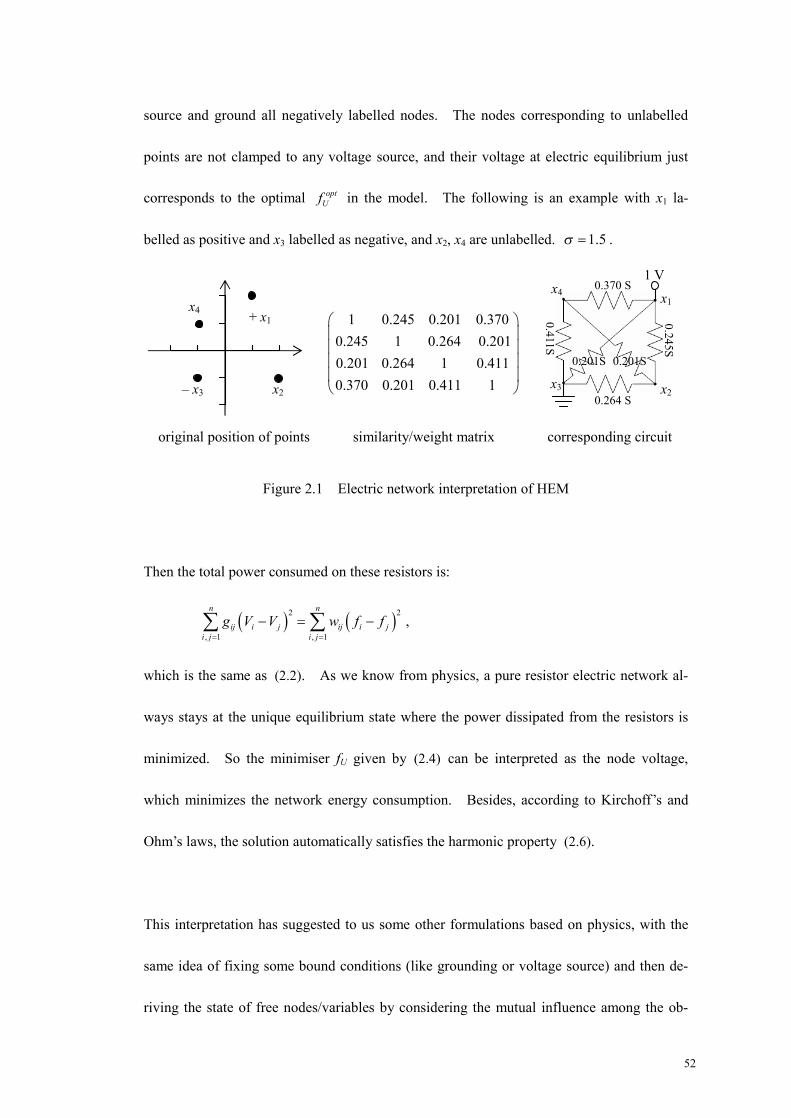
52
source and ground all negatively labelled nodes. The nodes corresponding to unlabelled
points are not clamped to any voltage source, and their voltage at electric equilibrium just
corresponds to the optimal optUf in the model. The following is an example with x1 la-
belled as positive and x3 labelled as negative, and x2, x4 are unlabelled. 1.5σ = .
1 0.245 0.201 0.3700.245 1 0.264 0.2010.201 0.264 1 0.4110.370 0.201 0.411 1
original position of points similarity/weight matrix corresponding circuit
Figure 2.1 Electric network interpretation of HEM
Then the total power consumed on these resistors is:
( ) ( )2 2
, 1 , 1
n n
ij i j ij i ji j i j
g V V w f f= =
− = −∑ ∑ ,
which is the same as (2.2). As we know from physics, a pure resistor electric network al-
ways stays at the unique equilibrium state where the power dissipated from the resistors is
minimized. So the minimiser fU given by (2.4) can be interpreted as the node voltage,
which minimizes the network energy consumption. Besides, according to Kirchoff’s and
Ohm’s laws, the solution automatically satisfies the harmonic property (2.6).
This interpretation has suggested to us some other formulations based on physics, with the
same idea of fixing some bound conditions (like grounding or voltage source) and then de-
riving the state of free nodes/variables by considering the mutual influence among the ob-
+ x1
x2
x4
– x3
x1
x2 x3
x4 0.370 S
0.264 S
0.201S 0.201S
0.245S
0.411S
1 V

53
jects in the whole system. We can replace the resistors with capacitors or inductors which
will lead to a time-sensitive exponential charging curve, similar to (Kondor & Lafferty,
2002). Furthermore, some electromagnetic induction models can be exploited as well.
However, this kind of models seems less well motivated in terms of machine learning theory.
So we put the next physics model into the next section, showing how the physics laws can
be used to motivate machine learning intuitions.
2.5 Interpreting HEM 3: Harmonic mean
The harmonic mean principle (2.6) is very appealing. It says that the value of a function f
at a point x should be equal to or close to the average value of f at other points in the prox-
imity of x, weighted by their similarity to x. This principle has been justified by the physi-
cal model of electric circuit. Now we show another interesting natural model which also
supports this principle. Suppose we introduce to the space some point charges of +Q or –Q
Coulomb. Each +Q or –Q point charge corresponds to a positively or negatively labelled
instance. They are insulated from everything else. Then we add into the space some
other grounded small metal spheres, which are also viewed as point charges. These corre-
spond to the unlabelled data. We know the mutual distance between all pairs of point
charges, which can be related to the weights of the graph G. As unlabelled point charges
are grounded, there will be some induced charges on them at static electric equilibrium.
Then whether these spheres have positive net charge or negative net charge will indicate
whether the data point is positive or negative.

54
As a simple example, we see how a single positive point charge elicits the induced charge on
a grounded point charge. Suppose the left insulated metal sphere has +Q. The right
grounded metal sphere has radius r and the distance between the centres of the two spheres
is d. Assuming that d r , we can view the spheres as point charges.
Figure 2.2 Static induction model for semi-supervised learning
The left +Q’s contribution to the right point’s potential is Q d . Suppose the right (unla-
belled) grounded point has q coulomb induced charge, then the fact that it is grounded en-
tails 0Q d q r+ = . Now suppose there are l insulated point charges each with charge
, iq Q Q∈ + − (i = 1, 2, …, l), and other u (unlabelled) grounded charges ql + 1, …, ql + u.
Let the radius of all points be r and the distance between point i and point j be dij ( )ijd r .
Then by the fact that the voltage of the unlabelled charges is 0, we have
1:
nji
j j i ij
qqr d= ≠
= − ∑ for all 1,...,i l l u= + + .
These u equations are very similar to the harmonic properties in (2.6), by replacing the ex-
ponential decaying with inverse linear decaying. The only caveat is the negative sign,
which people may attribute to the fact that like charges repel each other while opposite
charges attract. However, even if we manually change the rule to its opposite, the negative
sign will still be there, i.e., 0Q d q r+ = still holds for Figure 2.2. We omit the physics
details here. This model can be regarded as another natural instance of harmonic mean.
+ Q q – –
––
– –

55
2.6 Interpreting HEM 4: Graph kernels and heat/diffusion kernels
In section 2.2, we defined the graph Laplacian and used it just as a notation. We now study
the real role of this notion and then understand this model in a more profound way.
2.6.1 Preliminaries of graph Laplacian
Assume there is an undirected and unweighted graph G = ,V E , with vertex set V = 1...n ,
and edge set E. We write i ~ j ( i j≠ ) to denote that i and j are connected, i.e., (i, j)∈E, (j,
i)∈E. First define the adjacency matrix W: wij = 1 if i ~ j, and 0 otherwise. wii = 0. So
W is symmetric with diagonal values being 0. In a more general setting, we can extend wij
to [0, + ∞ ). Denote 1
ni ijj
d w=∑ for all i and assume that 0id > , i∀ . All the results
below, mainly from (Smola & Kondor, 2003), apply to this general definition of adjacency
matrix.
Now we define D as an n n× diagonal matrix with ii iD d . The transitional probability
matrix P of G, the combinatorial Laplacian ∆ , and normalized Laplacian ∆ are defined as
1P D W−= , ( )D W D I P∆ − = − , ( )1 1 1 12 2 2 2D D D D W D− − − −∆ ∆ = − (2.9)
respectively. Then we list some important properties of ∆ and ∆ with brief proof.
1. (Chung, 1997) ∆ and ∆ are both symmetric and positive semi-definite. The eigen-
values of ∆ are all real and in [0, 2] and the number of 0 eigenvalues is equal to the
number of disjoint components in G.
These bounds are straightforward from Gerschgorin’s Theorem (Chung, 1997).

56
2. (Smola & Kondor, 2003) If di is constant throughout all i (so denoted as d), then the re-
lationship between the eigenvalues and eigenvectors of ∆ , ∆ , and P is:
W P ∆ ∆
Eigenvalue λi λi / d d – λi 1 – λi / d
Eigenvector vi vi vi vi
Table 2.1 Relationship of eigen-system for graph matrices
If 1
nijj
w=∑ is not constant throughout all i, then there is no simple relationship. The
only surviving property is that P’s eigenvector vi corresponds to ∆ ’s eigenvectors12
iD v ,
and P’s eigenvalue λi corresponds to 1 – λi. This is because if i i iPv vλ= , then
( ) ( )1 1 1 1 1 1 12 2 2 2 2 2 21i i i i i iD v I D PD D v D v D Pv D vλ−∆ = − = − = − .
This result is useful because it is normally easier to calculate P than ∆ , particularly when
we need to take derivatives of them. As most important conclusions are expressed in terms
of the eigen-system of normalized ∆ , it will be convenient to study the theoretical proper-
ties in ∆ and then implement/calculate by using P in practice.
3. (Smola & Kondor, 2003) ∆ and ∆ can also be viewed as linear operators on func-
tions :V Rf . Let ( )1 2, ,..., Tnf f ff , then we can endow the functional space of
f with a semi-norm defined as the inner product between f and ∆ f :
( )22 12
~, T
ij i ji j
w f f∆
∆ = ∆ = −∑f f f f f for all n∈Rf . (2.10)
This semi-norm (since 2 0∆
=f iff f is a constant vector) depicts the weighted smooth-
ness of f on the n vertices.

57
4. (Chung, 1997) ∆ is a discrete approximation on the graph manifold of the Laplacian
operator 2 2 2
22 2 21 2 mx x x
∂ ∂ ∂∇ = + + +
∂ ∂ ∂ in continuous spaces.
First, the approximation relationship can be demonstrated by looking at an m-dimensional
lattice. Suppose the orthonormal bases are e1, …, em. x = x1e1 + … + xmem. where xi are
integers. Let ( )1 ,..., mx xf x = f . Then
( )2 f x∇ ( )( ) ( )1 1
2 22
1 1
i im m
i ix x
i ii
f x f xf x
x δ
∂ ∂∂ ∂
= =
+ − −∂= ≈
∂∑ ∑e e
( ) ( ) ( )2
1
2mi i
i
f x f x f xδ=
+ + − −≈ ∑
e e = [ ]2
1
1,..., mx xδ
− ∆ f .
Second, we show that Laplacian operator 2∇ also depicts the smoothness of f, but in a con-
tinuous compact space Ω :
( ) ( ) ( )2 2,f f f f f d f f d f dΩ Ω Ω
ω ω ω∆
= ∆ = ∆ = ∇ ⋅ ∇ = ∇∫ ∫ ∫ .
where a simple integral by part is applied. The meaning of smoothness by integrating
2f∇ is very clear because 2f∇ depicts the rate of local variance of f.
5. (Original work) If wij > 0 for all i, j, and S is a proper subset of V, then the eigenvalues
of SS∆ are in (0, 2), where SS∆ stands for the sub-matrix of ∆ restricted to S.
This property means the eigenvalues of SSI − ∆ are all in (–1, 1) and this is important to
prove the convergence of some processes to be discussed later. To prove it, we see now
the (i, i)th diagonal elements of SS∆ (not SS∆ ) is larger than the negative sum of all other
elements in the ith row of SS∆ , which we denote as dS,i. Denote SS SS SSD ′∆ + ∆ , where
Dss is a diagonal matrix and SS′∆ has the same off-diagonal elements as SS∆ , and its (i, i)th
diagonal element is dS,i. Therefore, Dss has a straight positive diagonal and it is positive

58
definite. By above property 1, we already know that SS′∆ is positive semi-definite. So
SS∆ is positive definite and its eigenvalues are all positive. By definition (2.9), SS∆ is
also positive semi-definite.
To prove that the eigenvalues of SS∆ are all less than 2, we only need to show that
2 SSI − ∆ or ( )2 SSD − ∆ is positive definite, where ( )2 SSD − ∆ stands for the submatrix of
2D − ∆ restricted to S. The proof is similar to the above one, except that we now use the
fact that 2D D W− ∆ = + is positive semi-definite. We restrict on S which results in
weakening of the off-diagonal, yielding a positive definite matrix in consequence.
We will relax the condition of wij > 0 into the assumption that there exists a path from every
node in S to a certain node in V \ S in section 4.4.1.
2.6.2 Graph and kernel interpretation 1: discrete time soft label summation
(Original work) We propose considering the following process. Suppose at the beginning
t = 0, the u unlabelled points have soft labels 0Uf . Then at time t, the average of other
points’ soft labels weighted by their similarity to xi is: 1: 1:
u ut
ij j ijj j i j j i
w f w= ≠ = ≠∑ ∑ . So we update
the tif by:
1
1: 1:
u ut t t t t
i i i ij j ij ij j i j j i
f f w f w fδ+
= ≠ = ≠
− = −∑ ∑ , (2.11)
which bears clear resemblance to some basic forms of neural network update with tiδ being
the difference between the weighted neighbours’ average and tif itself. Sometimes,

59
1t t ti i if f ηδ+ − = is used where (0, 1]η ∈ . We simplify (2.11) into:
1
1: 1:
u ut t
i ij j ijj j i j j i
f w f w+
= ≠ = ≠
← ∑ ∑ for t = 0, 1, … (2.12)
Now we have 1t tU UU Uf P f+ = , where
1
nij ij ijj
p w w=
= ∑ (wii = 0 by definition). We define
the final determinant soft label as the sum of the soft labels over all t:
( )0 0
0 0 0
t t tU U UU U UU U
t t tf f P f P f
+∞ +∞ +∞
= = =
= =
∑ ∑ ∑ . (2.13)
We first need to show that this definition converges. Recall the property 5 in section 2.6.1.
We know that the eigenvalues of UUI − ∆ are in (–1, 1). So ( )0
t
UUt
I+∞
=
− ∆∑ converges.
Moreover, as 1 12 2I D PD−∆ = − and D is diagonal, we have
1/ 2 1/ 2UU UU UU UUI D P D−− ∆ = , (2.14)
and ( ) ( )1/ 2 1/ 2t tUU UU UU UUI D P D−− ∆ = , ( )1/ 2 1/ 2 0tt
U UU UU UU Uf D I D f−= − ∆ for all t = 0, 1, ….
Thus 0
tUU
tP
+∞
=∑ ( )1/ 2 1/ 2
0
t
UU UU UUt
D I D+∞
−
=
= − ∆
∑ (then eigen-decompose UUI − ∆ )
1/ 2 1/ 2
0 1
ut T
UU i i i UUt i
D Dλ φ φ+∞
−
= =
=
∑∑ ( 1iλ < , so summation is interchangeable)
( ) 11/ 2 1/ 2 1/ 2 1/ 2
1 0 11
u ut T T
UU i i i UU UU i i i UUi t i
D D D Dλ φ φ λ φ φ+∞
−− −
= = =
= = −
∑∑ ∑
( )( ) 11/ 2 1/ 2 1/ 2 1 1/ 2UU UU UU UU UU UUD I I D D D
−− − −= − − ∆ = ∆
( ) ( )1 11/ 2 1/ 2 1/ 2 1/ 2UU UU UU UU UU UUD I D P D D I P
− −− −= − = − . (2.15)
So, Uf is well defined by (2.13) and the exact value is ( ) 1 0U UU Uf I P f−= − . (2.16)
Note although the final result of (2.15) is not surprising, we can not derive it directly be-
cause there is no guarantee that the infinite summation will converge. We can also make
use of the property 2 in section 2.6.1 to derive the result. Comparing with (2.4), we have
0U UL Lf P f= , which can be simply modelled by propagating the labels of fL to the u unlabelled

60
points through probability PUL.
2.6.3 Graph and kernel interpretation 2: continuous time soft label integral
(Original work) As a straightforward extension to continuous time soft label integral, we
modify (2.11) and define the dynamic system as:
( ) 1/ 2 1/ 2t t tU UU U UU UU UU Uf I P f D D f
t−∂
= − − = − ∆∂
. (2.17)
Let 1/ 2t tU UU Ug D f , then (2.17) becomes
t tU UU Ug g
t∂
= −∆∂
. (2.18)
This is the typical heat diffusion equation, whose solution uses the exponentiated matrix:
( ) 0exptU UU Ug t g= − ∆ . (2.19)
The matrix ( )exp UUt− ∆ is exactly the diffusion kernel proposed by (Kondor & Lafferty,
2002). Its (i, j)th element can be visualized as the quantity of some substance that would
accumulate at vertex xj after a given amount of time t if we injected the substance at vertex xi
at time 0 and let it diffuse through the graph along the edges according to the conductivity
defined by UU∆ .
Now the final soft label is defined by
Uf ( )1/ 2 1/ 2 0 1/ 2 1 0
0 0 0expt t
U UU U UU UU U UU UU Ut t tf dt D g dt D t dt g D g
+∞ +∞ +∞− − − −
= = == = − ∆ ⋅ = ∆∫ ∫ ∫
( ) ( )1 11/ 2 1/ 2 1/ 2 1/ 2 0 0UU UU UU UU UU U UU UD D I P D D f I P f− −− −= − = − (2.20)
which is the same as (2.16).
(Zhu et al., 2003a) pointed out that the HEM model is different from many time-dependent

61
models such as diffusion kernels in (Kondor & Lafferty, 2002) and fixed step Markov ran-
dom walks in (Szummer & Jaakkola, 2001). Now we find that the difference is just be-
cause HEM summed/integrated out the time t for the soft labels.
2.7 Interpreting HEM 5: Laplacian equation with Dirichlet Green’s functions
(Zhu et al., 2003a) pointed out the relationship of the harmonic energy minimization model
with the discrete Laplace equation with Dirichlet boundary conditions, solved by using
Green’s function (Chung & Yau, 2000). The Laplace equation is defined as:
( ) ( ) ( )( ) ( )1
u
xyy
f x f x f y p g x=
∆ = − =∑ for all x U∈ ,
and the Dirichlet boundary condition is defined as
( ) ( ) xf x x fσ= = for all x L∈ .
Here ( )f x is interpreted as the expected hard label of the first hit labelled point. So
( ) xy yy L
g x w f∈∑ for all x U∈ . According to the Theorems 1 and 2 in (Chung & Yau,
2000), the solution can be written as:
( ) ( ) [ ]1/ 2 1/ 2
1 ,0
1
xy
u
x i y z i zi x U y Li
p
f z d x f d Ggφ φλ
− −
= ∈ ∈≠
= +
∑ ∑ for all z U∈ ,
where iλ and iφ are the eigenvalues and eigenvectors of UU∆ , and G is the Green’s
function of I – PUU. After calculation, we find ( ) 1U UL L UU UL Lf GP f I P P f−= = − .
2.8 Applying matrix inversion lemma
In this section, we see how matrix inversion lemma can be utilized for active learning, in-

62
ductive learning and leave-one-out cross validation model selection. Active learning is
efficiently combined with semi-supervised learning in the framework of HEM through the
application of matrix inversion lemma and marginal Gaussian distribution formulation (Zhu
et al., 2003c). We mention these algorithms because they rely on the matrix inversion
lemma, an indispensable tool to make our later hyperparameter learning algorithm tractable.
Only the first section active learning is by (Zhu et al., 2003c) and the rest are original work.
2.8.1 Active learning
First of all, the true risk ( )fR of harmonic function f is defined as:
( ) ( )( ) ( )1 0,1
sgn * |i
n
i i ii y
f f y p y Lδ= =
≠∑ ∑R ,
where sgn( fi ) is the decision rule, e.g., sgn( fi ) = 1 if fi > 0.5 and 0 otherwise. p*(yi | L) is
the unknown and incomputable true posterior label distribution at node i given L. Assume
( )* 1|ip y L= if≈ , which is very similar to self-training assumptions, then the estimated
risk becomes ( ) ( )( )( ) ( )( ) ( )1 1
ˆ sgn 0 1 sgn 1 min ,1n n
i i i i i ii i
f f f f f f fδ δ= =
≠ − + ≠ = −∑ ∑R .
Now suppose we query the unlabelled node xk and expect to receive answer yk, then after
re-training with (xk, yk), there will be a new harmonic function ( , )k kx yf + , whose estimated
risk will be: ( ) ( )( , ) ( , ) ( , )
1
ˆ min , 1k k k k k k
nx y x y x y
i ii
f f f+ + +
=
= −∑R . However we still do not
know yk so we assume that ( )* 1|k kf p y L≈ = and calculate the expected estimated risk:
( ) ( ) ( ) ( )( ,0) ( ,1)ˆ ˆ ˆ1k k kx x xk kf f R f f R f+ + += − +R ,
And finally the query kopt chosen is: ( )ˆarg min kxoptkk R f += .
There are two computationally intensive steps and the approaches proposed to tackle them
63
are interesting. Firstly, we need to calculate ( , )k kx yf + :
( , ) 1\ , \ \ ,
k kx yU k U k U k L k L kf f+ −= −∆ ∆ ,
where 1\ , \U k U k
−∆ is the matrix after removing the kth row and kth column from UU∆ . Na-
ïvely inverting the matrix and multiplying matrix and vector for all k = 1…u will be very
costly. The crucial observation is that fU (its original meaning as a random variable noted
immediately after (2.5), while most of the time we used it as a shorthand for optUf ) conforms
to a Gaussian distribution with mean 1UU UL Lf−−∆ ∆ and covariance 1
UU−∆ . ( , )k kx yf + is con-
ditioning this Gaussian distribution on fk = yk, and calculating the posterior mean. There is
a direct formula proved using Schur complement in (Jordan, preprint):
( )( , ) 1 1( ) ( )k kx yU k k UU Uk UU kkf f y f+ − −= + − ∆ ∆ (2.21)
where 1( )UU Uk−∆ is the kth column of 1
UU−∆ and 1( )UU kk
−∆ is the (k, k)th element of 1UU−∆ .
So ( , )k kx yf + can be calculated in only ( )O u time.
Secondly, if we want to select one more query after querying xk and getting the answer yk,
then it is necessary to calculate the inverse of \ , \U k U k∆ , a matrix removing the kth column
and kth row from UU∆ . Consider k = 1 for instance. To calculate 1\1, \1U U
−∆ , we only need
to calculate the inverse of 11
\1, \1
00UU
U U
∆ ′∆ = ∆
, since ( )1
1 111\1, \1
00UU
U U
−−
−
∆′∆ = ∆
.
But UU′∆ is different from UU∆ only by the 1st row and 1st column, so there exist two vec-
tors kα and kβ , such that T TUU UU u ue eα β′∆ = ∆ + + , where eu = (1, 0, …, 0)T u∈R . The
matrix inversion lemma in its most primitive form says for any two vectors s and t,
( )1 11 1
1
TT
T
A s t AA st As At
− −− − ⋅+ = −
+ (as long as A + stT is invertible, i.e., 1 0Ts At+ ≠ ).
Therefore we can first invert TUU ue α∆ + on top of UU∆ by viewing eu as s and α as t.

64
Then we invert T TUU u ue eα β∆ + + on top of T
UU ue α∆ + by viewing β as s and eu as t.
In sum, the computational cost is O(u2).
2.8.2 Inductive learning
In contrast to active learning where the major computational cost stems from inverting a
matrix after removing one row and one column, the bottleneck of inductive learning is to
invert a matrix after adding one row and one column. Still, the key tool is matrix inversion
lemma.
Suppose the learner is given an unseen data xn+1. Then we just need to calculate the new fU:
1 1( 1), ( 1) ( 1),
nxU U n U n U n L Lf f++ −
+ + += −∆ ∆ .
The matrix ( 1), ( 1)U n U n+ +∆ is just adding one row and one column to UU∆ :
, 1( 1), ( 1)
1, 1, 1
UU U nU n U n
n U n n
++ +
+ + +
∆ ∆ ∆ = ∆ ∆
. (2.22)
We can invert ( 1), ( 1)U n U n+ +∆ efficiently because we can apply matrix inversion for two
times like in active learning on top of matrix 1, 1
00UU
n n+ +
∆ ∆
, whose inverse is
1
11, 1
00UU
n n
−
−+ +
∆ ∆
. So in sum, the cost for classifying an unseen data is O(u2+ul) = O(nu).
2.8.3 Online learning
For inductive learning, the unseen data is forgotten once it is classified and the prediction for
the upcoming unseen data is not affected by the previously (seen) unseen data. However,
the online learning in this model can make use of these data. We consider two settings.

65
1. The classifier is given the correct label of an unseen data immediately after it makes the
prediction. So now the ΔUU is fixed while ΔUL and fL grow. The cost for computing
1UU UL Lf−−∆ ∆ increases linearly to the number of unseen data s at O(u2+u(l+s)).
2. The classifier does not know the correct label of an unseen data even after it outputs the
prediction. Now we can update ΔUU in a run, so that it grows larger and larger with
more and more unseen data. Since the computational cost for updating ΔUU and com-
puting 1UU UL Lf−−∆ ∆ is O(nu), it is acceptable in many cases. If there are s unseen data,
then the total cost is O(u2+(u+1)2+…+(u+s)2+ul+(u+1)l+…+(u+s)l) = O(nsu+ns2+s3).
2.8.4 Leave-one-out cross validation
Leave-one-out cross validation (LOOCV) is usually an effective way for model selection.
In the semi-supervised setting, this means for each i L∈ , we view xi as an unlabelled point
and do transductive learning together with the pool of unlabelled data to get the soft label of
xi. Then we pick the model which makes the soft label maximally tally with the correct
class (i.e., maximally close to 1 for positive data and maximally close to 0 for negative data),
averaged over all i L∈ .
Although the scarcity of labelled data assumed in semi-supervised learning makes LOOCV
less justified by common theory, it is still an advisable way for model selection. The most
prominent difficulty lies in computational cost, as the model must be retrained for l times.
Since each training takes O(u3+ul), the total cost will be high O(lu3+ul2). By virtue of ma-
trix inversion lemma, we can reduce the total cost to O(nu2+ul3), which is more managable
66
given l u .
Again, the key idea is to look at the bottleneck of computation: matrix inversion. When xi
is held out from L, the ΔUU is augmented by adding one row and one column, whose values
correspond to xi. Similar to what we have already discussed for (2.22), the new augmented
matrix ,U i U i∆ can be inverted efficiently.
2.8.5 Two serious cautions
The simplicity of (2.21) offers not only delight, but also a serious caution: an algorithm may
be unexpectedly not using unlabelled data at all, though the optimization is formulated as if
it were semi-supervised learning.
The idea in (2.21) is that for a multivariate Gaussian distribution, if we condition on one
variable, then the mean of the other variables can be simply calculated by scaling the corre-
sponding columns in the covariance matrix. Putting it on a more concrete footing, suppose
there is a Gaussian distributed random vector ( ),TT T
L Ux x with mean ( ),TT T
L Uµ µ and co-
variance matrix LL LU
UL UU
Σ Σ Σ = Σ Σ
. Then the conditional probability ( )|U Lp x x is a
Gaussian distribution with mean ( )1U UL LL L Lxµ µ−+ Σ Σ − , and covariance 1
UU UL LL LU−Σ − Σ Σ Σ .
Now suppose we parameterize the covariance matrix directly, with each (i, j)th element de-
termined only by xi and xj only. Then each element in the mean vector
( )1U UL LL L Lxµ µ−+ Σ Σ − will just depend on the corresponding row in ULΣ . This is equiva-

67
lent to classifying the unlabelled data one by one, without exploiting their mutual relation-
ship or mutual help. The HEM avoided this trap by parameterizing the inverse covariance
matrix. In a more general picture, this phenomenon can also occur when regularizing by a
directly parameterized kernel K (e.g., yTK–1y), where K is playing a similar role as covari-
ance matrix as illustrated in Figure 2.3.
Figure 2.3 Relationship between graph Laplacian, kernel, and covariance matrix
The second caution is about overfitting in LOOCV. It seems surprising because LOOCV is
designed just to avoid it. However unwise and intensive use of LOOCV can overfit. How?
In http://www.autonlab.org/tutorials/overfit10.pdf, Andrew Moore used an example for il-
lustration. Imagine there is a dataset with 50 records and 1000 attributes. We try 1000
linear regression models, each one using one of the attributes. The best of those 1000 looks
good. But we realize it would have looked good even if the output had been purely random!
The solution proposed therein is: hold out an additional test set before doing any model se-
lection. Check the best model that performs well even on the additional test set. Or, use
randomization testing.
graph Laplacian
kernel matrix covariance matrix
Inverse Inverse
Equivalent

68
Chapter 3 Graph Hyperparameter Learning
So far, all the algorithms are assuming that the graph of pairwise similarity measure is given.
However, it is usually difficult to find a good graph. Using the kernel view of the HEM,
constructing the graph is of the same importance as choosing a kernel function, which is also
still under current popular research. Interestingly, however, there have been few graph
learning algorithms published hitherto which interface directly to the raw data. As we
pointed out in section 1.5.2, there do exist some algorithms based on a given dis-
tance/similarity measure, i.e., dij between example i and j. Nonetheless, now our interest is
in learning the dij. If we use the Gaussian radial basis function as similarity measure, then
learning the bandwidth is very similar to feature selection.
In this chapter, we will first review the preliminary graph learning algorithm proposed in
(Zhu et al., 2003a), and a latest work by (Kapoor et al., 2005). The main part of this chap-
ter will be proposing a simple graph learning principle based on the idea of leave-one-out
cross validation. We call it leave-one-out hyperparameter learning (LOOHL). The pri-
mary contribution of the work is an efficient gradient calculation algorithm based on the
matrix inversion lemma. It significantly reduced the computational complexity, with
which most leave-one-out style learning algorithms are plagued.
3.1 Review of existing graph learning algorithms
In section 1.4, we reviewed some principles such as maximum margin and maximizing the

69
likelihood on labelled and unlabelled points. In (Kapoor et al., 2005), the problem is for-
mulated in a Bayes net framework and the graph is learned by evidence/likelihood maximi-
zation, at the cost of approximate inference and expensive EM optimization. In (Zhu et al.,
2003a), the spirit of maximum margin is adopted in a tailored form, called entropy minimi-
zation, to fit his HEM. We review these two approaches in this section before proposing
our graph learning algorithm in the next section.
3.1.1 Bayes network through evidence maximization
(a) (b)
Figure 3.1 Bayes network of hyperparameter learning
First of all, the HEM is formulated in the Bayes inference framework, as in Figure 3.1 (a).
We use double arrow from node ( fL, fU) to ( fL) and ( fU) to represent that the first node fully
determines the second and third nodes, which are actually just a subset of the first node.
Bayes network does not have an efficient mechanism to express that one variable determines
the joint distribution of two other variables, and this is the only choice. The fL are fixed to
the given labels. (XL, XU) and ( fL) are both observed, and we want to infer the distribution
of, and mean or MAP of fU. The only probabilistic edge is from (XL, XU) to ( fL, fU), param-

70
eterized by the similarity matrix and graph Laplacian ∆ with coefficients σ (e.g., RBF
bandwidth), and possible graph smoothing (e.g., eigen-transform ( )r ∆ on graph Laplacian
as reviewed in section 1.5.1.2) with coefficient δ, which is not used in original HEM (i.e.,
( )r ∆ = ∆ ). This conditional probability is defined as:
( ) ( )( ) ( )( )112| exp 0,Tp f X f f Nσ σ −∝ − ∆ = ∆ (3.1)
where ( ),TT T
L Uf f f . As the mean and MAP of a Gaussian distribution collapse, the re-
sulting soft label fU is just the same as the minimizer of (2.3):
( ) ( ) ( ) ( )2T T T TU UU U U UL L L LL Lf f f f f f f fσ σ σ σ∆ = ∆ + ∆ + ∆ . (3.2)
The important difference between transductive classification and graph learning is that the
former minimizes (3.2) with respect to (wrt) Uf by fixing σ , while the latter minimizes
wrt both Uf and σ . The latter can be optimized by first minimizing wrt fU, and then σ .
( ) ( ) ( )1optU UU UL Lf fσ σ σ−= −∆ ∆ , which gives
( ) ( ) ( ) ( ) ( )( )1T T TL LL UL UU UL Lf f f fσ σ σ σ σ−∆ = ∆ − ∆ ∆ ∆ .
Unfortunately, this will trivially push all 0σ → , 0ijw → and ( ) ( )2
, 1
n
ij i ji j
E f w f f=
= −∑
0→ . So the normalized graph Laplacian is necessary to make it work.
Like HEM, the above formulation also assumes that the labels are noiseless. To incorpo-
rate the noise, (Kapoor et al., 2005) suggested using the Bayes net in Figure 3.1 (b). The
difference from Figure 3.1 (a) is that the soft label f is no longer fixed to the observed hard
label t. The assumption (3.1) is still used, but there is a new noise assumption earlier used
71
for Gaussian process classification by (Kim & Ghahramani, 2004; Opper & Winther, 1998):
( )1 0
|0
i ii i
i i
f tp t f
f tε
ε− ≥
= <, where [0,1]ε ∈ stands for the noise level.
Note ( )|i ip t f depends on the soft label f only via its sign. This flipping likelihood is
different from other linear or quadratic slack in likelihood, and it is particularly desirable for
cases where label errors are far from the decision boundary (Kim & Ghahramani, 2004).
Now ( ) ( ) , ,L U LX X t are observed and ( ) ( ) , ,L U Uf f t are hidden. The parameters are
, , σ δ ε , and they are learned by maximizing the evidence likelihood of ( ), ,L U LP X X t
through EM algorithm. Note the variable tU is not the ancestor of any observed variable, so
it is marginalized out and thus has no influence on ( ), ,L U LP X X t . In the E-step, the pos-
terior q(fL, fU) is inferred by evidence propagation algorithm, while in the M-step the pa-
rameters are optimized by (approximate) gradient descent. Finally, to infer tU, we only
need to integrate out ( fL, fU).
The performance of this model and actually many other Gaussian process models are highly
dependent on the noise model. The learning and inference, which are usually intractable in
the exact form, are normally carried out in an approximate way. Difficulty also arises from
optimization over the graph smoothing coefficient δ (e.g., eigen-transform ( )r ∆ on graph
Laplacian). This can usually transform the eigenvalues λ to ( )2exp / 2σ λ , ( ) 1aI λ −− ,
or even more complicated ( ) 1cos / 4λπ − , etc. It is either impossible to calculate the exact
gradient wrt the parameters, or calculating the spectral transformed ( )r ∆ will be too ex-
pensive in every iteration. That is why (Kapoor et al., 2005) restricted the transform to the
72
simplest way: ( )r λ λ δ= + , which means transforming ∆ to Iδ∆ + .
3.1.2 Entropy minimization
An alternative graph learning approach is based on the maximum margin principle, in a form
tailored for HEM. The idea is to make the classification on unlabelled points as confident
as possible, with fL clamped to 0/1. In other words, the f value of an unlabelled point xi
should be either close to 1 or close to 0, instead of around 0.5. Since f is bounded by (0, 1),
this objective can be equivalently formulated as minimizing the entropy of fi:
( ) ( ) ( )log 1 log 1i i i i iH f f f f f= − − − −
The entropy is minimized when fi is either near 0 or 1 and maximized when fi is 0.5. So the
final objective function to minimize is:
( ) ( ) ( ) ( )( )1 1
1 1 log 1 log 1n n
i i i i ii l i l
H f H f f f f fu u= + = +
= − + − −∑ ∑ (3.3)
This idea is also used successfully in (Grandvalet & Bengio, 2004) and (Niu et al., 2005).
It is different from normal entropy maximization formulations, where there is a unique op-
timal solution. There can be an exponentially large number of entropy minimizing solu-
tions which suggests that the criterion may not work consistently. However, (Zhu et al.,
2003a) argued that since the fi are fixed on labelled points, the unlabelled points do not have
much freedom in assuming so many possible values, i.e., most of the low entropy labellings
are inconsistent with the labelled points. Unfortunately, they did not elaborate on this
claim and our experimental results show that this criterion often fails to learn a good graph.

73
This criterion also suffers from the risk of overfitting. First, the number of features may be
far larger than the number of labelled points and we can have considerable freedom to con-
struct the graph into any one we want. Second, even if the number of parameters is small,
there is still a trivial solution which yields entropy 0, when 0dσ → . The bandwidth is so
small that ( )' 'ij ijw w j j≠ , where xj is the nearest neighbour of xi. So pij is close to 1
and ' 0ijp ≈ for all 'j j≠ and 'j i≠ . This results in the following procedure:
1. For each point in the labelled point set x, label its nearest unlabelled point with the same
label as x;
2. Add that unlabelled point to the labelled point set, and repeat from 1.
This procedure does give a minimum entropy labelling, but it is obviously undesired unless
the classes are perfectly separated.
The solution proposed in (Zhu et al., 2003a) in to add a uniform distribution regularizer, in-
spired by the work in PageRank algorithm (Ng et al., 2001b). They simply replace P with
( )1P Pε ε+ −U (3.4)
where U is the uniform matrix 1ij n−=U . This ensures that the graph is always fully con-
nected. Numerically, this smoothing is also necessary to make the optimization proceed
properly because in practice the transition matrix I – P quickly becomes close to singular if
we do not use this smoothing. However, (Zhu et al., 2003a) did not say whether (3.4) is
also used in classification, or just used in learning the graph. In experiments, we find that
graph P performs consistently better than P , so we stick to P when doing final classifica-
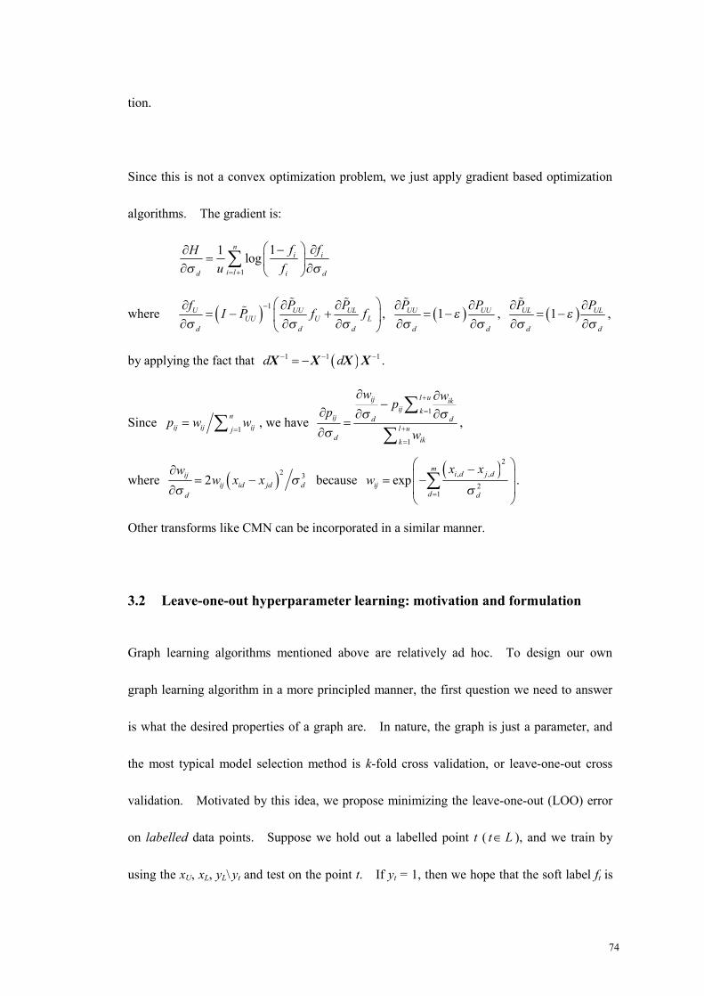
74
tion.
Since this is not a convex optimization problem, we just apply gradient based optimization
algorithms. The gradient is:
1
11 logn
i i
i ld i d
f fHu fσ σ= +
− ∂∂= ∂ ∂
∑
where ( ) 1U UU ULUU U L
d d d
f P PI P f fσ σ σ
− ∂ ∂ ∂= − + ∂ ∂ ∂
, ( )1UU UU
d d
P Pε
σ σ∂ ∂
= −∂ ∂
, ( )1UL UL
d d
P Pε
σ σ∂ ∂
= −∂ ∂
,
by applying the fact that ( )1 1 1d d− − −= −X X X X .
Since 1
nij ij ijj
p w w=
= ∑ , we have 1
1
l uij ikij k
ij d dl u
d ikk
w wpp
wσ σ
σ
+
=
+
=
∂ ∂−
∂ ∂ ∂=
∂
∑
∑,
where ( )2 32ijij id jd d
d
ww x x σ
σ∂
= −∂
because ( )2
, ,2
1exp
mi d j d
ijd d
x xw
σ=
− = −
∑ .
Other transforms like CMN can be incorporated in a similar manner.
3.2 Leave-one-out hyperparameter learning: motivation and formulation
Graph learning algorithms mentioned above are relatively ad hoc. To design our own
graph learning algorithm in a more principled manner, the first question we need to answer
is what the desired properties of a graph are. In nature, the graph is just a parameter, and
the most typical model selection method is k-fold cross validation, or leave-one-out cross
validation. Motivated by this idea, we propose minimizing the leave-one-out (LOO) error
on labelled data points. Suppose we hold out a labelled point t ( t L∈ ), and we train by
using the xU, xL, yL\ yt and test on the point t. If yt = 1, then we hope that the soft label ft is

75
as close to 1 as possible and if yt = 0, then we hope that the ft is as close to 0 as possible.
Note this rule can be easily made independent of the classification algorithms. Using the
random walk view, this is equivalent to the motivation that a particle leaving from a posi-
tively labelled point is expected to first hit (and absorbed by) another positively labelled
point with as high probability as possible. Then we want to maximize the sum or product
of these leave-one-out posterior probabilities.
Now we present the detailed formulation of leave-one-out hyper-parameter learning. In
this section, as the math equations are pretty complex, we write in a slightly verbose style to
help understanding by controlled redundancy. Suppose we examine the case when the tth
labelled data point is held out. Denote
tt tUtUU
Ut UU
p pP
p P
, ( )t L∈
where ( )1, ,,...,T
Ut l t n tp p p+ , ( ), 1 ,,...,tU t l t np p p+ ,
1 , 1 , 1
1,1 1, 1 1, 1 1,
,1 , 1 , 1 ,
t t t t t tl
l l t l t l ltUL
n n t n t n l
p p p pp p p p
P
p p p p
− +
+ + − + + +
− +
,
( )1 1 1,..., , ,..., TtL t t lf f f f f− + ,
( ) ( ) 1
1, ,..., Tt t t tU t l n UU UL Lf f f f I P P f
−
+ = − ,
where P is just applying (3.4) to P.
The LOO prediction on the held out tth labelled point is the first component of tUf , so the

76
0 0.1 0.2 0.3 0.4 0.5 0.6 0.7 0.8 0.9 10
0.1
0.2
0.3
0.4
0.5
0.6
0.7
0.8
0.9
1
0 0.1 0.2 0.3 0.4 0.5 0.6 0.7 0.8 0.9 10
0.1
0.2
0.3
0.4
0.5
0.6
0.7
0.8
0.9
1
0 0.1 0.2 0.3 0.4 0.5 0.6 0.7 0.8 0.9 10.2
0.3
0.4
0.5
0.6
0.7
0.8
0.9
1
0 0.1 0.2 0.3 0.4 0.5 0.6 0.7 0.8 0.9 10.2
0.3
0.4
0.5
0.6
0.7
0.8
0.9
1
0 0.1 0.2 0.3 0.4 0.5 0.6 0.7 0.8 0.9 10
0.1
0.2
0.3
0.4
0.5
0.6
0.7
0.8
0.9
1
0 0.1 0.2 0.3 0.4 0.5 0.6 0.7 0.8 0.9 10
0.1
0.2
0.3
0.4
0.5
0.6
0.7
0.8
0.9
1
objective function to be maximized is:
( ) 1
,11 1
l lt T t t t
t U t UU UL Lt t
Q c f c s I P P f−
= =
= = −∑ ∑ , (3.5)
where ( ) 11,0,...,0 T us += ∈R , and ct is the class of the tth example taking value in –1/+1 (not
0/1) corresponding to negative/positive respectively.
In addition to linear sum of ,1t
t Uc f , there can be other loss functions for each labelled point
based on ,1t
Uf . For example:
positively labelled negatively labelled
linear:
loss = 1 – f loss = f
exponential:
loss = a – f (a > 1) loss = a f – 1 (a > 1)
polynomial:
loss = (1 – f )a (a > 1) loss = f a (a > 1)
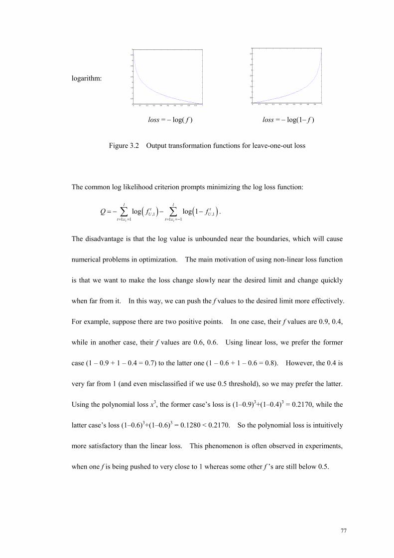
77
0 0.1 0.2 0.3 0.4 0.5 0.6 0.7 0.8 0.9 10
0.5
1
1.5
2
2.5
3
3.5
4
4.5
5
0 0.1 0.2 0.3 0.4 0.5 0.6 0.7 0.8 0.9 10
0.5
1
1.5
2
2.5
3
3.5
4
4.5
5
logarithm:
loss = – log( f ) loss = – log(1– f )
Figure 3.2 Output transformation functions for leave-one-out loss
The common log likelihood criterion prompts minimizing the log loss function:
( ) ( ),1 ,11: 1 1: 1
log log 1t t
l lt t
U Ut c t c
Q f f= = = =−
= − − −∑ ∑ .
The disadvantage is that the log value is unbounded near the boundaries, which will cause
numerical problems in optimization. The main motivation of using non-linear loss function
is that we want to make the loss change slowly near the desired limit and change quickly
when far from it. In this way, we can push the f values to the desired limit more effectively.
For example, suppose there are two positive points. In one case, their f values are 0.9, 0.4,
while in another case, their f values are 0.6, 0.6. Using linear loss, we prefer the former
case (1 – 0.9 + 1 – 0.4 = 0.7) to the latter one (1 – 0.6 + 1 – 0.6 = 0.8). However, the 0.4 is
very far from 1 (and even misclassified if we use 0.5 threshold), so we may prefer the latter.
Using the polynomial loss x3, the former case’s loss is (1–0.9)3+(1–0.4)3 = 0.2170, while the
latter case’s loss (1–0.6)3+(1–0.6)3 = 0.1280 < 0.2170. So the polynomial loss is intuitively
more satisfactory than the linear loss. This phenomenon is often observed in experiments,
when one f is being pushed to very close to 1 whereas some other f ’s are still below 0.5.

78
To make use of non-linear optimization packages, we need to calculate the partial deriva-
tives of Q with respect to the hyperparameters. Assuming
( )2
, ,2
1exp
mi d j d
ijd d
x xw
σ=
− = −
∑ ,
the partial derivatives are:
( ) ( ) ( )1 1 1
1
t tlT t t t t t tUU UL
t UU UU UL L UU Ltd d d
P PQ c s I P I P P f I P fσ σ σ
− − −
=
∂ ∂∂= − − + − ∂ ∂ ∂
∑
( ) ( ) 1
11
t tlT t t tUU UL
t UU U Lt d d
P Pc s I P f fεσ σ
−
=
∂ ∂= − − + ∂ ∂
∑
where the fact that ( )1 1 1d d− − −= −X X X X is applied as in the section 3.1.2. Since in the
original matrix P, 1
nij ij ikk
p w w=
= ∑ , we have
1
1
l uij ikij k
ij d dl u
d ikk
w wpp
wσ σ
σ
+
=
+
=
∂ ∂−
∂ ∂ ∂=
∂
∑
∑.
Finally, ( )2 32ijij id jd d
d
ww x x σ
σ∂
= −∂
. (3.6)
Note the equation (3.6) also indicates the generality of our algorithm in terms of the para-
metric form of similarity measures, as long as the measure is non-negative and continuous.
We may safely replace the Gaussian RBF form with polynomial form or tanh, and the only
change is the partial derivative in (3.6).
For convenience, we assume ε = 0 in the rest part of the chapter, and then P P= . It is
easy to extend the following techniques to ε > 0.

79
The pseudo-code below calculates the gradient for the leave-one-out hyperparameter learn-
ing in a very naïve way.
1. Function value: F = 0; Gradient: g = (0, …, 0)T m∈R .
2. For each 1...t l= (leave-one-out loop)
,t t tUtUU
Ut UU
p pP
p P
←
, ( )1, ,,...,T
Ut l t n tp p p+= and ( ), 1 ,,...,tU t l t np p p+= , (3.7)
1 , 1 , 1
1,1 1, 1 1, 1 1,
,1 , 1 , 1 ,
t t t t t tl
l l t l t l ltUL
n n t n t n l
p p p pp p p p
P
p p p p
− +
+ + − + + +
− +
←
, (3.8)
( ) 1t t t tU UU UL Lf I P P f
−← − , (3.9)
( ) 1T t t tt UU UL LF F c s I P P f
−← + − . (3.10)
Let tUUW and t
ULW be the weight matrix with the same index corresponding to tUUP
and tULP . We will denote the (i, j)th element of t
UUW as ( , )tUUw i j . We use
1
( , )tnUN
k d
w i kσ=
∂∂∑ and
1( , )n t
UNkw i k
=∑
to denote the sum of the elements in the ith row of t t
UU UL
d d
W Wσ σ
∂ ∂ ∂ ∂
and ( )t tUU ULW W
respectively. In fact, by (3.7) and (3.8), regardless of the value of t, the 2nd row up to
the (u+1)th row of tUUW and t
ULW always corresponds to the u unlabelled points. The
first row (i=1) always corresponds to the labelled data point currently held out. So for
i = 1, 1
( , )tnUN
k d
w i kσ=
∂∂∑ and
1( , )n t
UNkw i k
=∑ are equal to the sum of the elements in the tth
row of d
Wσ
∂∂
and W respectively. For 2,..., 1i u= + , 1
( , )tnUN
k d
w i kσ=
∂∂∑ and
80
1( , )n t
UNkw i k
=∑ are equal to the sum of the elements in the (i + l – 1)th row of d
Wσ
∂∂
and
W respectively. This is an important property which we will utilize later.
3. For each d = 1…m (for all features inside the leave-one-out loop)
11
( , ) ( , ) ( , )1 ( , )( , )
t t tntUU UU UN
UUn ktd d dUNk
P i j w i j w i kp i jw i kσ σ σ=
=
∂ ∂ ∂← − ∂ ∂ ∂
∑∑
(3.11)
1... 1, 1... 1i u j u= + = +
11
( , ) ( , ) ( , )1 ( , )( , )
t t tntUL UL UN
ULn ktd d dUNk
P i j w i j w i kp i jw i kσ σ σ=
=
∂ ∂ ∂← − ∂ ∂ ∂
∑∑
(3.12)
1... 1, 1... 1i u j l= + = −
where ( , )tUL
d
w i jσ
∂∂
, if corresponds to the pth and qth example (indices of the
original W), equals ( )2 3, ,2 pq p d q d dw x x σ− .
( ) 1 t tT t t tUU UL
d d t UU U Ld d
P Pg g c s I P f fσ σ
− ∂ ∂← + − + ∂ ∂
(3.13)
End
End
The naïve algorithm is very computationally expensive: ( )( )2O lu mn u+ , just for calculat-
ing the gradient once. In detail, the calculation of W and P in (3.7) and (3.8) costs
( )2O mn . (3.9) and (3.10) cost ( )( ) ( )2 3 3O l lu u u O lnu lu+ + = + (matrix inversion costs
( )3O u ). (3.11) and (3.12) cost ( )O lmnu . (3.13) costs ( )O lmnu . To be more precise,
matrix inversion is known to have the same difficulty as matrix multiplication, which costs

81
( )2log 7O u ≈ ( )2.81O u by Strassen’s algorithm and ( )2.37O u by Winograd & Coppersmith’s
algorithm. See (Cormen et al., 2001) for details. So finally the complexity can be re-
duced to ( )( )1.37O lu mn u+ .
This high complexity is due to the following drawbacks:
1. The expensive matrix inversion is performed for l times, though the matrices to be in-
verted are only slightly different by the first row and first column.
2. It ignores the fact that for each example xi, there may be only a small number of fea-
tures whose value is nonzero (active features). This is particularly true for text or im-
age datasets.
3. In the leave-one-out loop, a lot of intermediate terms such as ( , )tUU
d
P i jσ
∂∂
and ( , )t
UL
d
P i jσ
∂∂
are repeatedly calculated which constitutes a considerable waste. A careful
pre-computation of common terms is desirable to reduce the cost.
3.3 An efficient implementation
By paying attention to the above three problems, we now propose an efficient implementa-
tion which helps to reduce the complexity to ( )2 2.37O mn lnu u+ + for calculating the gra-
dient, where m is the average of mutually active features:
1
2 1... or is not zero on feature ( 1) i j
i j nm d m x x d
n n ≤ < ≤
∈− ∑ .
This is already close to the lower bound because it is inevitable to calculate

82
( )2 32ijij id jd d
d
ww x x σ
σ∂
= −∂
(for , 1...i j u= , 1...d m= ), particularly ( )2
id jdx x− which
can not be further factorized. Although ( )2
id jdx x− is constant throughout all iterations,
we can not pre-compute it because the cost for storing the result is 2( )O u m , usually beyond
the memory capacity. The following describes the factorization procedure which yields the
computational cost ( )2 2.37O mn lnu u+ + for gradient calculation.
The first expensive step is matrix inversion, which costs ( )3O lu . To start with, we use
matrix inversion lemma to reduce its cost to a one-time full matrix inversion and then some
( )2O u operations for l – 1 times. In (3.7) and (3.9), the matrix to be inverted is tUUI P− .
For different t, only the first row and first column of tUUP are different. In essence, we
only need to efficiently invert a u u× matrix T TB A e eα β= + + , where A–1 is known.
Here α and β are two vectors and e = (1, 0, …, 0)T 1u+∈R . By matrix inversion lemma,
( )1 11 1
1
TT
T
A AA AA
α βαβ
α β
− −− − ⋅+ = −
+
we can invert TA eα+ and then T TA e eα β+ + in ( )2O u time.
However, we still cannot avoid inverting a full matrix for t = 1. Therefore, the cost of (3.9)
has been reduced to ( )2 2.37O lu u+ , while (3.10) costs ( )O lnu . So (3.9) and (3.10) cost
( )2.37O lnu u+ in sum.
The second expensive step is in (3.11), (3.12) and (3.13), particularly by the partial de-
rivatives:
83
11
( , ) ( , ) ( , )1 ( , )( , )
t t tntUU UU UN
UUn ktd d dUNk
P i j w i j w i kp i jw i kσ σ σ=
=
∂ ∂ ∂= − ∂ ∂ ∂
∑∑
11
( , ) ( , ) ( , )1 ( , )( , )
t t tntUL UL UN
ULn ktd d dUNk
P i j w i j w i kp i jw i kσ σ σ=
=
∂ ∂ ∂= − ∂ ∂ ∂
∑∑
( ) 1 t tT t t tUU UL
d d t UU U Ld d
P PG G c s I P f fσ σ
− ∂ ∂← + − + ∂ ∂
Examining them carefully,
( , )ttUU
Ud
P i fσ
∂ ⋅∂
1
1
( , ) ( , )1 ( , )( , )
t tnt tUU UU
UU Un ktd dUNk
w i w i kp i fw i k σ σ=
=
∂ ⋅ ∂= − ⋅ ∂ ∂
∑∑
1
1
( , ) ( , )1 ( , )( , )
t tnt t tUU UN
U UU Un ktd dUNk
w i w i kf p i fw i k σ σ=
=
∂ ⋅ ∂= − ⋅ ⋅ ∂ ∂
∑∑
(3.14)
where ( , )tUU
d
w iσ
∂ ⋅∂
and ( , )tUUp i ⋅ are interpreted as row vectors covering all proper indices
for the “ ⋅ ”, restricted by tUUP . Here we have lifted out
1
( , )tn UNk
d
w i kσ=
∂∂∑ as common fac-
tor by making use of the fact that this term in the definition of ( , )tUU
d
P i jσ
∂∂
is independent of
j. Note tULP also has such property which will be utilized as well:
( , )ttUL
Ld
P i fσ
∂ ⋅∂ 1
1
( , ) ( , )1 ( , )( , )
t tnt tUL UN
UL Ln ktd dUNk
w i j w i kp i j fw i k σ σ=
=
∂ ∂= − ∂ ∂
∑∑
1
1
( , ) ( , )1 ( , )( , )
t tnt t tUL UN
L UL Ln ktd dUNk
w i w i kf p i fw i k σ σ=
=
∂ ⋅ ∂= − ⋅ ⋅ ∂ ∂
∑∑
. (3.15)
Now we look at the computational cost of each term in (3.14).
1. W and P. It costs ( )2O mn to calculate W and P.
2. 1
( , )n tUNk
w i k=∑ costs ( )O n for a given i, ( )O nu to cover all i. But it costs only
( )2O n to cover all t, because for different t, the 2nd row up to the (u + 1)th rows are un-
changed. Formally, for all 2... 1i u= + , 2... 1j u= + , and any 1 2t t≠ :

84
1 2( , ) ( , )t tUU UUw i j w i j= and ( ) ( ) ( ) ( )1 1 2 2
1 1 1 1
1 1 1 1, , , ,
u l u lt t t tUU UL UU UL
k k k kw i k w i k w i k w i k
+ − + −
= = = =
+ = +∑ ∑ ∑ ∑ .
3. 1
( , )tn UNk
d
w i kσ=
∂∂∑ costs ( )O mn for a given (i, t) (with all the nonzero features in either
xi or xk already covered), and ( )O mnu to cover all i. Since only the first row and first
column of tUUW change for different t, it costs ( )( ) ( )2O mn u l O mn+ = to cover all t.
4. ( , )t tUU Up i f⋅ costs ( )O u for fixed i and t, so it costs ( )2O u to cover all i. Although
the second row up to the (u + 1)th row of tUUp are unchanged for different t, the t
Uf
changes completely with t. So it still costs ( )2O lu to cover t.
5. ( , )ttUU
Ud
w i fσ
∂ ⋅∂
costs ( )O mu , with all the nonzero features in xi already covered. So it
costs ( )2O mu to cover all i and ( )2O lmu to cover all t. This will be too expensive.
Fortunately, with t changing, ( , )tUU
d
w iσ
∂ ⋅∂
is basically constant: only the first row and
first column change with t. So we just need to record the tUf for all t L∈ and then
traverse all items in ( , )tUU
d
w iσ
∂ ⋅∂
only once (in contrast to l times). In this way, the cost
to cover all i and t is ( )O mnu .
We summarize the costs below and underline the bottleneck computational terms.
( , )ttUU
Ud
P i fσ
∂ ⋅∂
1
1
( , ) ( , )1 ( , )( , )
t tnt t tUU UN
U UU Un ktd dUNk
w i w i kf p i fw i k σ σ=
=
∂ ⋅ ∂= − ⋅ ⋅ ∂ ∂
∑∑
(3.14)
with i, t fixed to cover all i to cover all t
W, P ( )2O mn ( )2O mn ( )2O mn
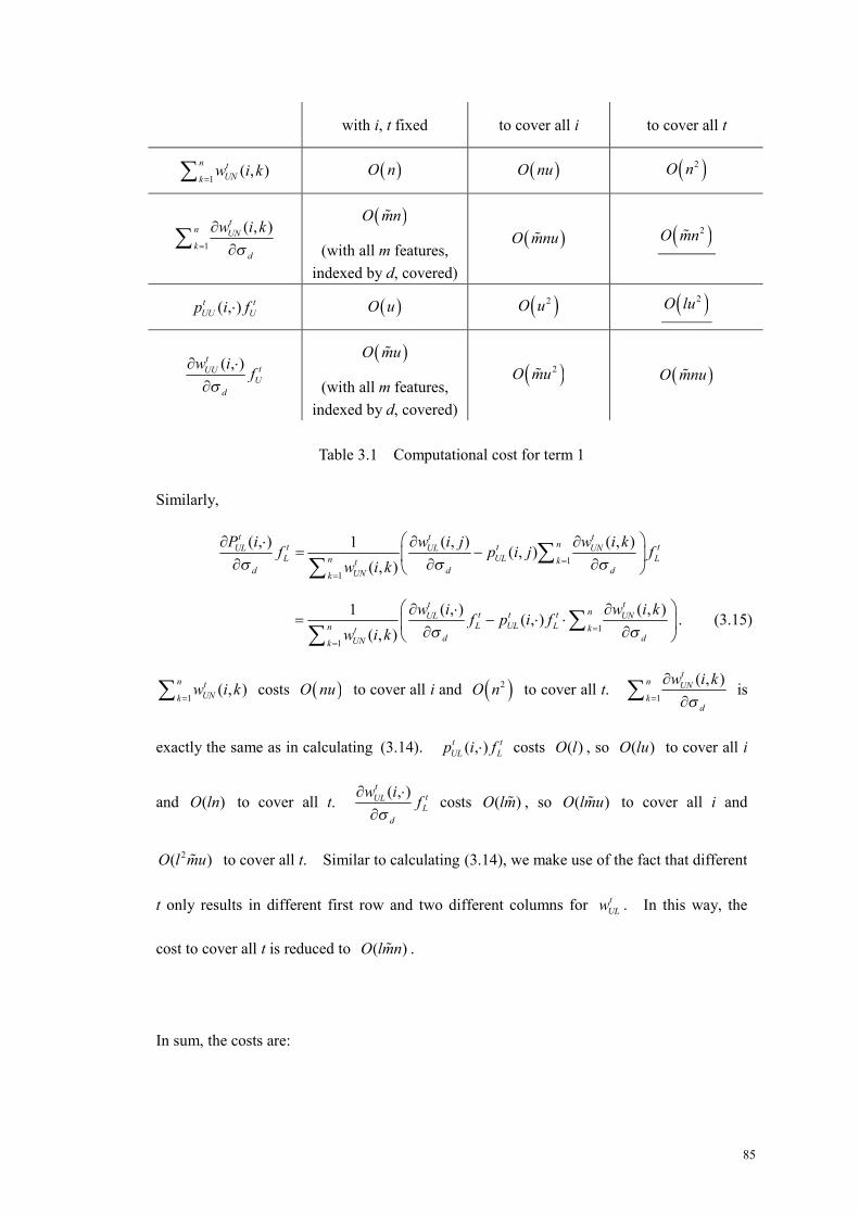
85
with i, t fixed to cover all i to cover all t
1( , )n t
UNkw i k
=∑ ( )O n ( )O nu ( )2O n
1
( , )tn UNk
d
w i kσ=
∂∂∑
( )O mn
(with all m features, indexed by d, covered)
( )O mnu ( )2O mn
( , )t tUU Up i f⋅ ( )O u ( )2O u ( )2O lu
( , )ttUU
Ud
w i fσ
∂ ⋅∂
( )O mu
(with all m features, indexed by d, covered)
( )2O mu ( )O mnu
Table 3.1 Computational cost for term 1
Similarly,
( , )ttUL
Ld
P i fσ
∂ ⋅∂ 1
1
( , ) ( , )1 ( , )( , )
t tnt tUL UN
UL Ln ktd dUNk
w i j w i kp i j fw i k σ σ=
=
∂ ∂= − ∂ ∂
∑∑
1
1
( , ) ( , )1 ( , )( , )
t tnt t tUL UN
L UL Ln ktd dUNk
w i w i kf p i fw i k σ σ=
=
∂ ⋅ ∂= − ⋅ ⋅ ∂ ∂
∑∑
. (3.15)
1( , )n t
UNkw i k
=∑ costs ( )O nu to cover all i and ( )2O n to cover all t. 1
( , )tn UNk
d
w i kσ=
∂∂∑ is
exactly the same as in calculating (3.14). ( , )t tUL Lp i f⋅ costs ( )O l , so ( )O lu to cover all i
and ( )O ln to cover all t. ( , )ttUL
Ld
w i fσ
∂ ⋅∂
costs ( )O lm , so ( )O lmu to cover all i and
2( )O l mu to cover all t. Similar to calculating (3.14), we make use of the fact that different
t only results in different first row and two different columns for tULw . In this way, the
cost to cover all t is reduced to ( )O lmn .
In sum, the costs are:

86
( , )ttUL
Ld
P i fσ
∂ ⋅∂ 1
1
( , ) ( , )1 ( , )( , )
t tnt t tUL UN
L UL Ln ktd dUNk
w i w i kf p i fw i k σ σ=
=
∂ ⋅ ∂= − ⋅ ⋅ ∂ ∂
∑∑
(3.15)
with i, t fixed to cover all i to cover all t
W, P ( )2O mn ( )2O mn ( )2O mn
1( , )n t
UNkw i k
=∑ ( )O n ( )O nu ( )2O n
1
( , )tn UNk
d
w i kσ=
∂∂∑
( )O mn
(with all m features,
indexed by d, covered)
( )O mnu ( )2O mn
( , )t tUL Lp i f⋅ ( )O l ( )O lu ( )O ln
( , )ttUL
Ld
w i fσ
∂ ⋅∂
( )O lm
(with all Fm features
already covered)
( )O lmu ( )O lmn
Table 3.2 Computational cost for term 2
So the overall computational cost is
( )2 2.37O mn lnu u+ + . (3.16)
This is already close to the lower bound, due to the inevitable cost of calculating W and P.
The memory cost is not the bottleneck and it depends on implementation. The lower bound
is ( )2O n , just to store W and P. In our implementation, we only used a constant number
of n m× matrices, for each index (i, d) of 1
( , )tn UNk
d
w i kσ=
∂∂∑ .

87
3.4 A mathematical clarification of the algorithm
The above analysis is rather intuitive and complicated. We wish to give a neat mathemati-
cal form which clearly shows the computational cost. Note this mathematical formulation
will not further reduce the cost, because the algorithm’s complexity has already reached its
lower bound. However, the artifice we adopt in the following math equations will also be
applied in the next chapter to calculate the gradient of the regularizers.
Combining (3.11), (3.14) and (3.15), we find that what we really need to compute is:
( ) 1
1
t tlT t t tUU UL
t UU U Lt d d
P PQ c s I P f fσ σ
−
=
∂ ∂= − + ∂ ∂
∑
where ( , )ttUU
Ud
P i fσ
∂ ⋅∂ 1
1
( , ) ( , )1 ( , )( , )
t tnt t tUU UN
U UU Un ktd dUNk
w i w i kf p i fw i k σ σ=
=
∂ ⋅ ∂= − ⋅ ⋅ ∂ ∂
∑∑
( , )ttUL
Ld
P i fσ
∂ ⋅∂ 1
1
( , ) ( , )1 ( , )( , )
t tnt t tUL UN
L UL Ln ktd dUNk
w i w i kf p i fw i k σ σ=
=
∂ ⋅ ∂= − ⋅ ⋅ ∂ ∂
∑∑
.
Let ( )( )1 Tt T t
t UUc s I Pβ−
− . Expanding the equations above, we have
Q ( )
( ) ( )1 1 1
, ,1 1 1 1
1
, ,
,
t ttl u u lUU ULt ti
U j L jn tt i j jd dUNk
w i j w i jf f
w i kβ
σ σ
+ + −
= = = ==
∂ ∂= + ∂ ∂
∑∑ ∑ ∑∑
( ) ( ) ( )1 1
, ,1 1 1
,, ,
tn u lUN t t t t
UU U j UL L jk j jd
w i kp i j f p i j f
σ
+ −
= = =
∂− + ∂ ∑ ∑ ∑ (3.17)
1 1
n nij
iji j d
wα
σ= =
∂
∂∑∑ .
The crucial idea is to pre-compute ijα , which is independent of the feature d. Then we
perform the following operations at computational cost ( )2O mn :
For i, j = 1…n
For all feature d which is nonzero in either xi or xj
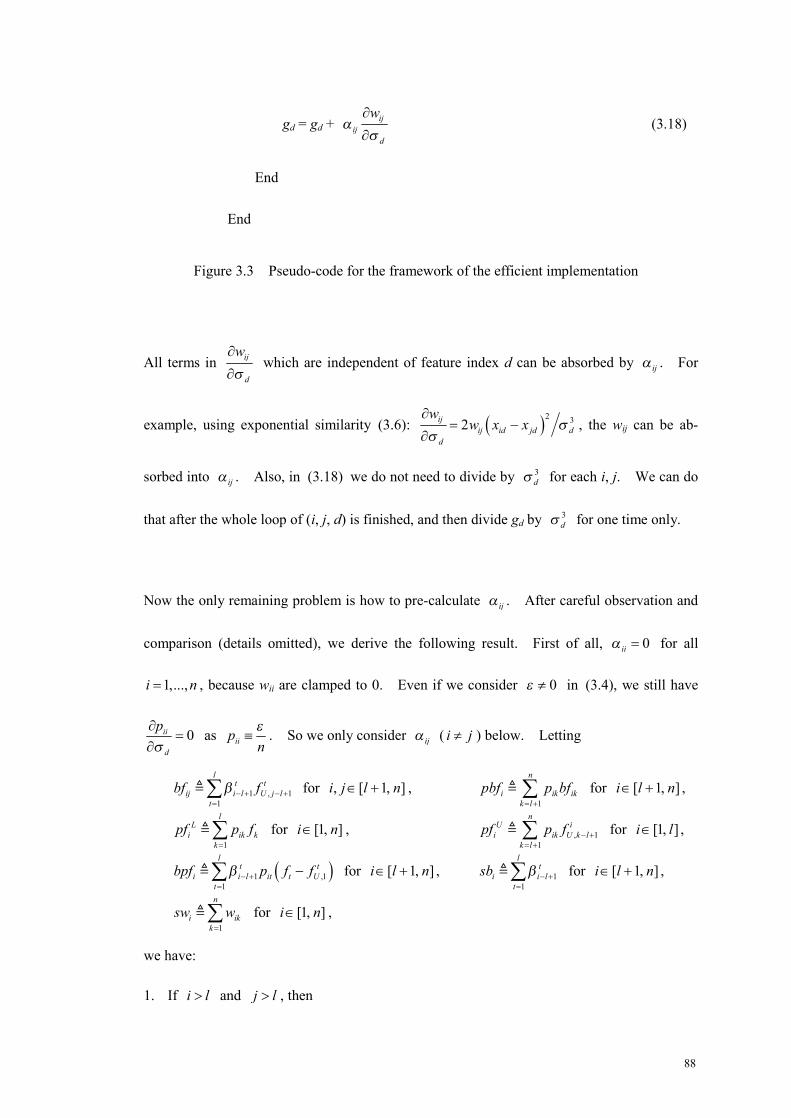
88
gd = gd + ijij
d
wα
σ∂
∂ (3.18)
End
End
Figure 3.3 Pseudo-code for the framework of the efficient implementation
All terms in ij
d
wσ
∂
∂ which are independent of feature index d can be absorbed by ijα . For
example, using exponential similarity (3.6): ( )2 32ijij id jd d
d
ww x x σ
σ∂
= −∂
, the wij can be ab-
sorbed into ijα . Also, in (3.18) we do not need to divide by 3dσ for each i, j. We can do
that after the whole loop of (i, j, d) is finished, and then divide gd by 3dσ for one time only.
Now the only remaining problem is how to pre-calculate ijα . After careful observation and
comparison (details omitted), we derive the following result. First of all, 0iiα = for all
1,...,i n= , because wii are clamped to 0. Even if we consider 0ε ≠ in (3.4), we still have
0ii
d
pσ
∂=
∂ as iip
nε
≡ . So we only consider ijα ( i j≠ ) below. Letting
1 , 11
lt t
ij i l U j lt
bf fβ − + − +=∑ for , [ 1, ]i j l n∈ + ,
1
n
i ik ikk l
pbf p bf= +∑ for [ 1, ]i l n∈ + ,
1
lL
i ik kk
pf p f=
∑ for [1, ]i n∈ , , 11
nU i
i ik U k lk l
pf p f − += +∑ for [1, ]i l∈ ,
( )1 ,11
lt t
i i l it t Ut
bpf p f fβ − +=
−∑ for [ 1, ]i l n∈ + , 11
lt
i i lt
sb β − +=∑ for [ 1, ]i l n∈ + ,
1
n
i ikk
sw w=
∑ for [1, ]i n∈ ,
we have:
1. If i l> and j l> , then

89
ijα ( ) ( )1 1
1, 1 , ,
1 1 11
1, 1,tl u l
t t t t ti lU j l UU U k UL L kn
t k kikk
f p i l k f p i l k fw
β + −− +
− += = =
=
= − − + − − +
∑ ∑ ∑
∑
1 , 1 , 1 ,11 1 1:
1
1 l n lt t t ti l U j l ik U k l it U ik kn
t k l k k tikk
f p f p f p fw
β − + − + − += = + = ≠
=
= − − −
∑ ∑ ∑
∑
1 , 1 1 , 11 1 1
1 l l nt t t ti l U j l i l ik U k l
t t k li
f p fsw
β β− + − + − + − += = = +
= −
∑ ∑ ∑
1 ,1 1 11 1 1 1
l l l lt t t ti l it U i l ik k i l it t
t t k tp f p f p fβ β β− + − + − +
= = = =
− − +
∑ ∑ ∑ ∑
( )1 , 1 1 , 1 1 ,1 11 1 1 1 1 1
1 l n l l l lt t t t t t ti l U j l ik i l U k l i l it t U i l ik k
t k l t t t ki
f p f p f f p fsw
β β β β− + − + − + − + − + − += = + = = = =
= − + − −
∑ ∑ ∑ ∑ ∑ ∑
1
1 nL
ij ik ik i i ik li
bf p bf bpf sb pfsw = +
= − + − ⋅
∑
( )1 Lij i i i i
i
bf pbf bpf sb pfsw
= − + − ⋅ .
2. If i l> and j l≤ , then
ijα ( ) ( )1 ,1 , 1 ,11 1 1:
1
1 l n lt t t ti l U j ik U k l it U ik kn
t k l k k tikk
f t j f t j p f p f p fw
β δ δ− + − += = + = ≠
=
= = + ≠ − − −
∑ ∑ ∑
∑
( )1 ,1 1 1 , 1 1 ,11 1 1
1 l n lt j j t t t ti l U i i l j i l ik U k l i l it U
t k l ti
f sb f p f p fsw
β β β β− + − + − + − + − += = + =
= + − − −
∑ ∑ ∑
1 11 1 1
l l lt ti l ik k i l it t
t k tp f p fβ β− + − +
= = =
− +
∑ ∑ ∑
( )( )1 ,11 j j L
i j i l U j i i i ii
sb f f f pbf bpf sb pfsw
β − += + − − + − ⋅ .
where ( )conditionδ is 1 when the condition is met and is 0 otherwise.
3. If i l≤ and j l> , then only when t = i will (3.17) make any contribution to ijα .
ijα ( ) ( )1 1
1, 1 , ,
1 11
1, 1,i u l
i i i i iU j l UU U k UL L kn
k kikk
f p k f p k fw
β + −
− += =
=
= − −
∑ ∑
∑
1, 1 ,1 , 1
1 1:1
i n li i i
U j l ii U ik U k l ik knk l k k iikk
f p f p f p fw
β− + − +
= + = ≠=
= − − −
∑ ∑
∑

90
1, 1 , 1
1 11
i n li i
U j l ik U k l ik knk l kikk
f p f p fw
β− + − +
= + ==
= − −
∑ ∑
∑ (note pii = 0)
( )1, 1
ii U L
U j l i ii
f pf pfswβ
− += − − .
4. If i l≤ and j l≤ , then
ijα ( ) ( )1,1 , 1
1 11
i n li i
U j ik U k l ik knk l kikk
f i j f i j p f p fw
βδ δ − +
= + ==
= = + ≠ − −
∑ ∑
∑
( )1i
U Lj i i
i
f pf pfswβ
= − − (for i j≠ ).
All ijbf , ipbf , Lipf , U
ipf , ibpf , isb , isw can be computed within ( )2O lu time, so all
these ijα can be pre-computed in ( )2O lu time, with memory cost ( )2O n . The overall
computational cost is ( )2 2.37O lnu n m u+ + , including matrix inversion at ( )2.37O u , tUf at
( )O lnu , ijα at ( )2O lu , and (3.18) at ( )2O mn . This is our final result and it is the same
as the conclusion in (3.16).
As a final note, we can apply this mathematical artifice to the implementation of entropy
minimization in section 3.1.2. Using (3.3),
( ) ( )( )1
1 log 1 log 1n
i i i ii l
H f f f fu = +
−= + − −∑ .
1
11 logn
Ti i U
i ld i d d
f f fH su fσ σ σ= +
− ∂ ∂∂= = ∂ ∂ ∂
∑ ,
where 1
1
1 11 log ,..., logT
l n
l n
f fsu f f
+
+
− −
.
( ) 1u UU ULUU U L
d d d
f P PI P f fσ σ σ
− ∂ ∂ ∂= − + ∂ ∂ ∂
. Let ( ) 1TUUr I P s
−= − , then
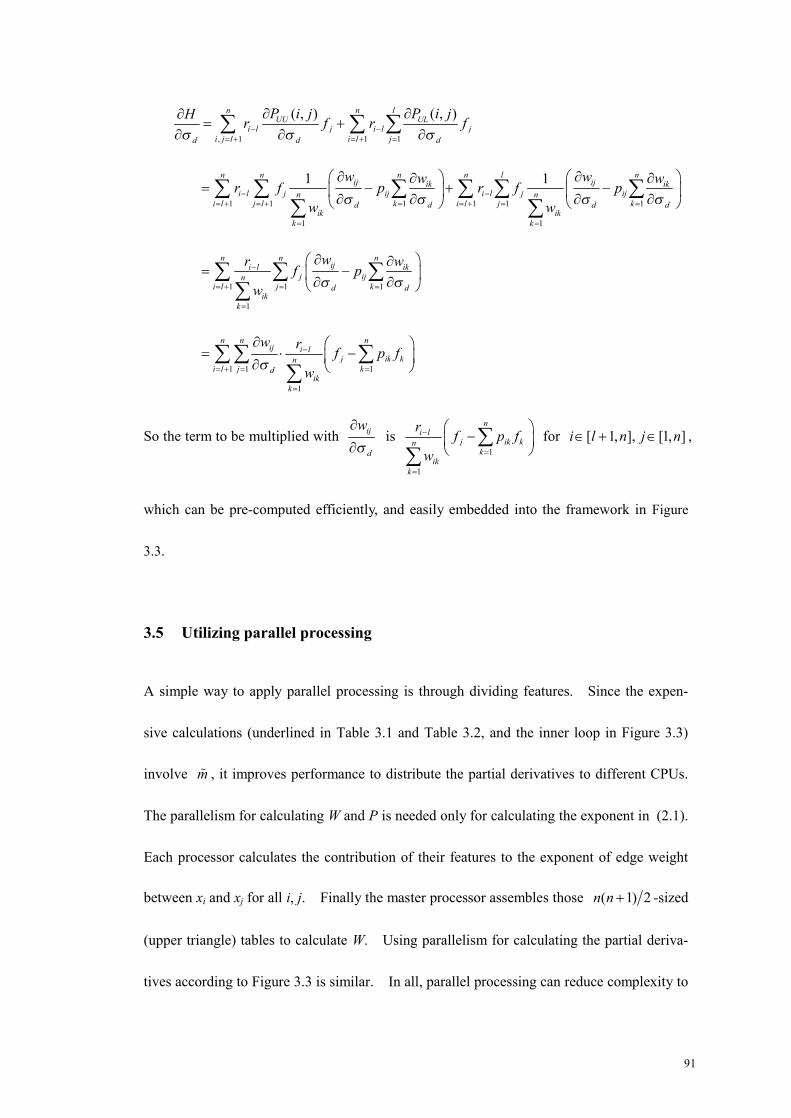
91
, 1 1 1
( , ) ( , )n n lUU UL
i l j i l ji j l i l jd d d
P i j P i jH r f r fσ σ σ− −
= + = + =
∂ ∂∂= +
∂ ∂ ∂∑ ∑ ∑
1 1 1 1 1 1
1 1
1 1n n n n l nij ijik ik
i l j ij i l j ijn ni l j l k i l j kd d d d
ik ikk k
w ww wr f p r f pw wσ σ σ σ− −
= + = + = = + = =
= =
∂ ∂ ∂ ∂= − + − ∂ ∂ ∂ ∂
∑ ∑ ∑ ∑ ∑ ∑∑ ∑
1 1 1
1
n n niji l ik
j ijni l j kd d
ikk
wr wf pw σ σ−
= + = =
=
∂ ∂= − ∂ ∂
∑ ∑ ∑∑
1 1 1
1
n n nij i l
j ik kni l j kd
ikk
w r f p fwσ−
= + = =
=
∂ = ⋅ − ∂
∑ ∑ ∑∑
So the term to be multiplied with ij
d
wσ
∂
∂ is
1
1
ni l
j ik knk
ikk
r f p fw
−
=
=
−
∑
∑ for [ 1, ], [1, ]i l n j n∈ + ∈ ,
which can be pre-computed efficiently, and easily embedded into the framework in Figure
3.3.
3.5 Utilizing parallel processing
A simple way to apply parallel processing is through dividing features. Since the expen-
sive calculations (underlined in Table 3.1 and Table 3.2, and the inner loop in Figure 3.3)
involve m , it improves performance to distribute the partial derivatives to different CPUs.
The parallelism for calculating W and P is needed only for calculating the exponent in (2.1).
Each processor calculates the contribution of their features to the exponent of edge weight
between xi and xj for all i, j. Finally the master processor assembles those ( 1) 2n n + -sized
(upper triangle) tables to calculate W. Using parallelism for calculating the partial deriva-
tives according to Figure 3.3 is similar. In all, parallel processing can reduce complexity to

92
2( )O n m r , where r is the number of processors available.
Furthermore, how to divide the features into several sets is also a problem, if we want the load
on different processors to be balanced. Though this is an NP-hard problem, we only need an
approximate solution. Suppose we have a list of length m, each element recording
active( , , )d i ji j
a x x d= ∑∑ , where active( , , )i jx x d is 0 if neither xi nor xj is nonzero on feature
d. Otherwise, it is set to 1. So the problem is: given n examples, m features, and r processors,
find a partition of C = 1, 2, ..., m into A1, …, Ar ( 1rk kA C= = , i jA A φ= for i j∀ ≠ ),
such that ( )1...
maxk r
load k=
is minimized where ( )k
dd A
load k a∈
= =∑ ( , , )k
i jd A i j
active x x d∈∑ ∑∑ .
For simplicity, we only need to consider unlabelled xi and xj, because the leave-one-out loop
treats only one labelled data as unlabelled. Therefore, this sub-optimal partitioning needs to be
computed only once given the set of labelled and unlabelled examples.
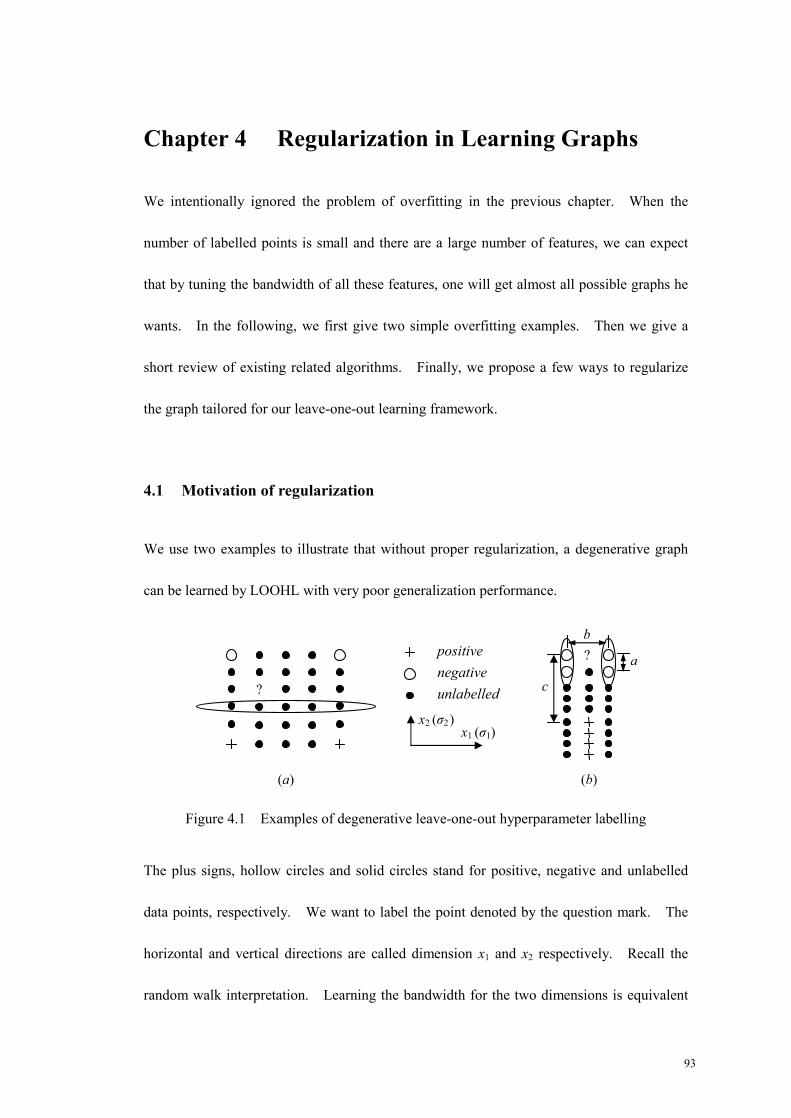
93
Chapter 4 Regularization in Learning Graphs
We intentionally ignored the problem of overfitting in the previous chapter. When the
number of labelled points is small and there are a large number of features, we can expect
that by tuning the bandwidth of all these features, one will get almost all possible graphs he
wants. In the following, we first give two simple overfitting examples. Then we give a
short review of existing related algorithms. Finally, we propose a few ways to regularize
the graph tailored for our leave-one-out learning framework.
4.1 Motivation of regularization
We use two examples to illustrate that without proper regularization, a degenerative graph
can be learned by LOOHL with very poor generalization performance.
Figure 4.1 Examples of degenerative leave-one-out hyperparameter labelling
The plus signs, hollow circles and solid circles stand for positive, negative and unlabelled
data points, respectively. We want to label the point denoted by the question mark. The
horizontal and vertical directions are called dimension x1 and x2 respectively. Recall the
random walk interpretation. Learning the bandwidth for the two dimensions is equivalent
?
(a)
?
(b)
a
b
c
x1 (σ1) x2 (σ2 )
positive negative unlabelled

94
to learning the tendency to walk horizontally or vertically, if equidistance. Suppose there
are three points W(a, b), X(a+1, b), Y(a, b+1). The particle is now at W. Then if band-
width σ1 is larger than σ2, it means that a point is more likely to walk horizontally (to X) than
vertically (to Y). When σ1 → +∞, points with the same x2 co-ordinate are effectively col-
lapsing into one point.
Now in example Figure 4.1 (a), the points of the same classes all have the same x2 coordi-
nate. For each labelled point, there is another labelled point from the opposite class which
has the same x1 coordinate. So the leave-one-out hyperparameter learning will push σ2 to
positive infinity, i.e., all points can transfer only horizontally. Therefore the graph will be
effectively divided into 6 groups, each with the same x2 coordinate. We showed one group
in Figure 4.1 (a). So this causes a problem. First the desired gradual change of labelling
from positive to negative along dimension x2 cannot appear. And as the point at question
mark can only transfer horizontally, it cannot hit any labelled point and cannot be classified.
In practice, any small numerical perturbation will cause it to be classified to an unforesee-
able class.
In Figure 4.1 (b), we assume a b c . Although the negative points will encourage
both horizontal and vertical walk, horizontal walk will make the leave-one-out soft label er-
ror large on positive points. So the learned σ2 will be far larger than σ1, i.e., strongly en-
courage walking vertically. As a result, the point at the question mark will be labelled as
positive, although by nearest neighbour intuition, it should be labelled as negative. Besides,
we notice that the four negative points will also be partitioned into two groups as shown in

95
the figure.
How to avoid these undesired behaviours will motivate different regularizers. We mention
some ideas below and we will develop them in the following sections. The first remedy is
through directly controlling σ, while the rest control σ indirectly by considering the property
of the resulting graphs.
1. Add square loss 2ii
σ∑ . However, the bandwidths obviously do not have a zero
mean Gaussian prior, so we need to modify it into ( )2ˆi iiσ σ−∑ , where ˆ iσ stands for
the prior mean, which can be assigned by cross validation under the original HEM al-
gorithm.
2. Modify transfer probability from pij to ( )/ 1 ijn pε ε+ − . This method will help con-
nect all nodes together and was used in (Zhu et al., 2003a).
3. Maximize the entropy of row transfer probability on unlabelled data points. Note this
entropy is not the posterior soft label entropy as used in section 3.1.2. It will prefer
more balanced (uniform) transfer probability distribution to other nodes, and it connects
each node to as many nodes as possible so that large clusters are formed. This will
encourage the unlabelled data in Figure 4.1 (a) and (b) to connect to more nodes in ver-
tical direction and horizontal direction respectively.
4. Minimize [ ]E t , the expected number of steps needed for a given unlabelled data to hit
a labelled point. In Figure 4.1 (a), [ ]E t is approaching infinity for all unlabelled
nodes not in the top or lowest x2 coordinate. In Figure 4.1 (b), [ ]E t for nodes near
the negative data can be reduced if the horizontal transfer is more encouraged.

96
5. Other means to encourage larger clusters, i.e., smaller number of clusters. We will use
spectral methods in section 4.3. In both examples in Figure 4.1, we can see the exis-
tence of small and separate clusters may harm the performance.
In section 4.2, we give a brief survey of the literature related to regularizing the complexity
of a graph. Due to the scarcity of existing work, such a relationship may seem far-fetched,
though one regularizer will be later motivated from clustering. After that we propose sev-
eral ad hoc regularizers based on above intuitively desirable properties of a graph.
4.2 How to regularize? A brief survey of related literature
To the best of our knowledge, there has been hardly any existing work that explicitly regu-
larizes the learning of the graphs. We call this task graph learning regularization instead
of graph regularization in order to avoid confusion with the graph Laplacian used for regu-
larizing the labelling (see section 1.5.1.2). Despite the lack of directly related literature, we
try to relate the graph learning problem to kernel learning and the desired properties in spec-
tral clustering. The latter view motivated one graph learning regularizer which will be pre-
sented in section 4.3.
4.2.1 Regularization from a kernel view
The first source of graph learning regularizer we have found is through the graph’s associa-
tion with kernels. Firstly, such an association is straightforward as described in section
1.5.1.2. Secondly, the theory of kernels is relatively mature and it offers a lot of conven-

97
ience to consider in the reproducing kernel Hilbert space (RKHS). Unfortunately, further
investigation reveals a disappointing fact that regularizers for learning kernels are scarce by
itself, though the theory of using kernels themselves to do regularization is abundant. The
most promising method is kernel learning, which is very popular recently. See for example,
(Lanckriet et al., 2004; Weinberger et al., 2004; Zhu et al., 2004; Kwok & Tsang, 2003;
Crammer et al., 2002; Cristianini et al., 2001). However, they all implicitly restrict the pa-
rametric form of the kernel, without explicit terms that penalize the complexity of the ker-
nels. This may cause problems in general. For example in (Lanckriet et al., 2004), learn-
ing kernels with only positive semi-definiteness constraints yields consistently inferior em-
pirical performance to learning from a positive combination of several fixed kernels, for
which semi-definite programming actually degenerates to quadratic programming. So how
to restrict the capacity of the candidate kernel set, or regularize the kernel learning, is still an
important and open problem even in the field of kernel learning.
(Ong et al., 2005; Ong & Smola, 2003) proposed an interesting measure of kernel space ca-
pacity called hyperkernels. In addition to the normal cost function terms such as the loss
function on labelled data, and the norm of the classification function in the RKHS induced
by the kernel K, it also includes a term which depicts the norm of that kernel K in the space
of candidate kernels, which is also a RKHS induced by a so-called hyperkernel. In that
way, there will be an additional penalty to choosing a complex kernel. This is exactly what
we want in our graph learning algorithms: how to measure and penalize the complexity of a
graph.

98
However, there are still three obstacles to using this method. Firstly, the optimization tech-
nique, semi-definite programming, is still not efficient enough for large scale datasets.
Secondly, in graph algorithms, we parameterize the graph Laplacian, which is the
pseudo-inverse of the associated kernel (see Figure 2.3). So it is indirect and inconvenient
to formulate, implement, and optimize (e.g., calculating gradient) the regularizer. Thirdly,
the proper forms of hyperkernel still leave much to be further studied.
4.2.2 Regularization from a spectral clustering view
We introduced the idea of spectral graphical clustering in section 1.5.1.3. We now develop
it in detail. From section 1.5.1.3, we know the (normalized) graph Laplacian contains use-
ful information of the graph’s clustering structure. The eigenvalues of the Laplacian and
normalized Laplacian play an important role. So if we want to design a regularizer relating
to the graph clustering structure, the eigenvalues will be a good choice of study.
Suppose the symmetric affinity matrix is W. The Laplacian is defined as D W∆ = − ,
where 1( ,..., )nD diag d d= with 1
0ni ijj
d w=
= >∑ . The normalized Laplacian is ∆ =
( )1/ 2 1/ 2D D W D− −− . By property 2 in section 2.6.1, the eigenvalues of ∆ are equal to
( )1P D D W−= − . So although the elements in ∆ are difficult to handle (square roots),
we only need to investigate P , which has the same eigenvalues as ∆ . By property 1 in
section 2.6.1, the eigenvalues of P lie in [0, 2] . In the following, we will only consider
( )112
P D D W−= + so that the eigenvalues lie in [0, 1] . The next question is what prop-
erty do we expect from the eigenvalues?

99
The following figures extracted from (Meilă & Shi, 2001) show two instances of eigenval-
ues’ distribution. The upper 20*20 images are the affinity (weight) matrices W and the
lower are the eigenvalues of P . The darker the pixel is, the smaller is the weight (ranging
in [0, 1] ). The range of y-axis in the lower two images is [0, 1] .
Figure 4.2 Eigenvalue distribution example of two images
P has a trivial eigenvalue 1, with eigenvector 1n
. Theoretically, if there are k mutually
disconnected components, then 1 should be an eigenvalue of P with multiplicity k. The
average of the rest eigenvalues is ( ) ( )/ 2n k n k− − , because the trace of P (the sum of
all eigenvalues) is / 2n if the diagonal of W is straight 0. ( ) ( )/ 2n k n k− − approaches
1/2 when n is large, and most of the eigenvalues not equal to 1 lie in [0, 0.5] . In the left
figure, there are roughly three clusters, and we can see three large eigenvalues which are far
away from the rest. In the right figure, some eigenvalues other than the largest three ei-
genvalues are rather close to them (decreasing slowly), which corresponds to the more am-
biguous clustering structure in the original W. So given that our objective is to encourage
1
0
1
0

100
the graph to be well clustered (reducing the inter-cluster similarity and increasing the in-
tra-cluster similarity), we wish to have some eigenvalues close to 1 and the rest eigenvalues
close to 0. The gap between these two groups of eigenvalues is expected to be as large as
possible. This is also in line with the concept of eigengap maximization in matrix pertur-
bation theory (Ng et al., 2001a; Stewart & Sun, 1990). Of course, we wish to restrict the
number of 1-valued eigenvalues as well, in order to avoid many small clusters.
In addition, we can also analyse through kernel PCA. ∆ can be viewed as the
pseudo-inverse covariance matrix, or the pseudo-inverse of the kernel. An eigenvalue
[0, 2]λ ∈ of ∆ is mapped to the eigenvalue 1 2λ− of P . So the above requirements
on P ’s eigenvalues can be translated as: the variance in the non-leading principal directions
should be small, or the difference of variance between leading and non-leading principal
directions should be large. This is also well known as an ideal property for the principal
components in the kernel space for denoising.
4.3 Graph learning regularizer 1: approximate eigengap maximization
Summarizing the ideas in section 4.2.2, the penalty function over eigenvalues may look like
Figure 4.3. The shape can be approximated by polynomials like ( )16 1x x− or other
( )1rx x− for large r’s. So the objective function is ( ) 1
1 1 11
n n nr r ri i i i
i i iλ λ λ λ +
= = =
− = −∑ ∑ ∑ . As
1
nri
iλ
=∑ is equal to the trace of rP , it is equivalent to minimizing the trace of 1r rP P +− .
Note the left tail covers 0.6 or so, because most non-principal eigenvalues average 0.5 and we
do not want to penalize over these eigenvalues. Of course, the exponent r can be adjusted

101
Figure 4.3 Example of penalty function over eigenvalues
so that the rising point can be shifted horizontally (see the three curves in Figure 4.3). The
only disadvantage is that the sharp decrease of penalty function near 1λ = may not be the
best choice. Fortunately, if we start from a graph which is not too disconnected, then most
eigenvalues are on the left tail of the curve. Minimizing the penalty by gradient descent
will just push them to the left, rather than climbing over the peak and decline in the right tail.
For more simplicity, we can just adopt penalty functions like
rλ (r ≥ 2), (4.1)
which is finally used in our experiments.
Calculating rP only costs log r times of matrix multiplication. Another computa-
tional advantage is that the partial derivatives are easy to calculate due to the special prop-
erty of trace: ( ) ( )1 Tr rtr rX
−∂=
∂X X , where X is a n n× matrix. So ( )r
d
trσ∂
=∂
X
1
, 1
nijr
jii j d
xr x
σ−
=
∂
∂∑ , where 1rjix − stands for the ( j, i)th element of X
r–1.
0 0.1 0.2 0.3 0.4 0.5 0.6 0.7 0.8 0.9 10
0.005
0.01
0.015
0.02
0.025
r = 16
r = 20
r = 24

102
Now we present the math formulae for calculating the objective function and its gradient.
Let 1P D W−= , then ( ) ( )( )( )2rrtr P tr I P= + . Specifically, when 2r = , ( )2tr P =
, 1 1
1 24
n n
ij ji iii j i
p p p n= =
+ +
∑ ∑ , which can be calculated in ( )2O n time. For 2r > , the Mat-
lab function mpower (mlfMpower in Matlab C Math Library) can be used to compute the
power by repeated squaring. Recall 1 1
n nij ij ik
ij ikk kd dd
p w wp wσ σσ = =
∂ ∂ ∂= − ∂ ∂∂
∑ ∑ , then we have
( )r
d
tr Pσ∂
∂ 1 1
, 1 , 1
12
n nij ijr r
ji jii j i jd d
p pr p r p
σ σ− −
= =
∂ ∂= =
∂ ∂∑ ∑
1
, 1 1 1
12
n n nijr ik
ji ij iki j k kd d
w wr p p wσ σ
−
= = =
∂ ∂= − ∂ ∂
∑ ∑ ∑
1 1
1 1 1
1
1 12
n n nij r r ik
ji ij jini j kd d
ikk
w wr p p pw σ σ
− −
= = =
=
∂ ∂= − ∂ ∂
∑ ∑ ∑∑
1 1
1 1 1
1
1 12
n n nij r r
ji ik kini j kd
ikk
wr p p p
wσ− −
= = =
=
∂ = − ∂
∑∑ ∑∑
So the factor to be multiplied with ij
d
wσ
∂
∂ is 1 1
1 1
12
n nr rji ik ki ik
k kr p p p w− −
= =
−
∑ ∑ , which can be
pre-computed efficiently. Note here that i and j vary from 1 to n, i.e., the whole graph
rather than restricted to unlabelled data. Finally, we just apply the framework in Figure
3.3.
4.4 Graph learning regularizer 2: first-hit time minimization
In this formulation, we consider the random walk interpretation under unsupervised setting.
For a particle starting to walk from an unlabelled data point i, it will take some steps to hit a

103
labelled data point, upon which it stops walking. Since the walk is random, we are con-
cerned about the average (expected) number of steps needed to hit a labelled point, denoted
as ai. The objective is to minimize the total average steps 1
nii l
a= +∑ defined on unlabelled
data only. To proceed, we first need to derive a mathematical form of 1
nii l
a= +∑ .
We have shown in section 2.3 that for 1,..., i U l n∈ = + , optif (defined in (2.4)) can be
interpreted as the probability that a particle starting from node i hits a positively labelled
data first. Now we go to more details and define tif as the probability that a particle
starting from node i hits a labelled data point within t steps (including t steps). It does not
matter whether the labelled data is positive or negative. Then
( ) ( )1 1
1 1 1 1 1
n n nt t t t
i i i i ii l i l t t i l
a t f f t f f+∞ +∞
− −
= + = + = = = +
= − = ⋅ −∑ ∑ ∑ ∑ ∑ (4.2)
and the objective function to be minimized is:
( )1
1 1 1
n nt t
i i ii l i l t
a t f f+∞
−
= + = + =
= −∑ ∑ ∑ . (4.3)
We can calculate the tif ( i U∈ ) recursively with ease:
1
1 11
0 0
l nt
ij ij jtj j li
p p f tf
t
−
= = +
+ ≥=
=
∑ ∑ (4.4)
where pij is the transition probability from i to j. The first question that should be answered
is whether the definition of ai in (4.2) is sound, i.e., does the summation converge? The
answer is yes, as long as some preconditions are met. Once it is proved to be theoretically
well defined, how to compute its value and gradient efficiently? The next sub-sections will
deal with the two questions respectively.

104
4.4.1 Theoretical proof and condition of convergence
Proposition 1.
1
nii l
a= +∑ converges if for each unlabelled point, there exists an edge to a certain la-
belled data point, i.e., 1
0l
ijj
p=
>∑ for all 1,...,i l n∈ + .
Proof. If this precondition is met, then we have
1max 1
n
iji U j lM p
∈ = +
<∑ . (4.5)
Let 1
1,...,maxM ii l n
f f∈ +
, and ( )1 1,1,...,1 T ss ∈R
for any natural number s.
1t ti if f −− 1 2
1 1 1 1
l n l nt t
ij ij j ij ij jj j l j j l
p p f p p f− −
= = + = = +
= + − +
∑ ∑ ∑ ∑ ( )1 2
1
nt t
ij j jj l
p f f− −
= +
= −∑
( )2 3
1 1
n nt t
ij jk k kj l k l
p p f f− −
= + = +
= −∑ ∑ =
= 1 1 2 2 1 1
1 2 1
1, , ,
, , ,t t t
t
i i i i i i ii i i U
p p p f− − −
− ∈∑
So ( )1
1
nt t
i ii l
f f −
= +
−∑ 0 1 1 2 2 1 1
0 1 1
1, , ,
, , , 1,...,t t t
t
i i i i i i ii i i l n
p p p f− − −
− ∈ +
= ∑
0 0 1 1 2 2 1
0 1 1
1, , ,
, , , 1,...,t t
t
i i i i i i ii i i l n
f p p p− −
− ∈ +
= ∑
( ) 1 11 tTu UU UP f−= ⋅ ⋅
(4.6)
where ( )1 1 1 11 2, , ,
T
U l l nf f f f+ + . Thus to prove that ( )1
1 1
nt t
i it i l
t f f+∞
−
= = +
⋅ −∑ ∑ converges, it suf-
fices to show that ( ) 1tUUP − 1 decays sufficiently faster (e.g., exponentially) than the linear
increase rate of t. This is guaranteed by the proposition’s precondition. By definition of
(4.5), each element in UUP is less than or equal to 1M (here, 1 is exponent, not super-
1 Note here t – 1 is exponent. To avoid confusion of superscript and exponent, we will not write 1t
UUP − , but always use parenthesis for power in this chapter.
105
script). Suppose in ( ) 1tUUP − , each element 1t
ijp − (t – 1 is superscript) is less than or equal
to 1tM − . Then the elements in ( )tUUP are 1
1
nt tij ik kj
k lp p p −
= +
= ∑ 1
1
nt
ikk l
p M −
= +
≤ ∑ 1
1
nt
ikk l
M p−
= +
= ∑
tM≤ . So by induction, we have proved that all elements in ( )tUUP are smaller or equal
to tM for all 1t ≥ . Continuing (4.6), we have
( )1 2 1
1
nt t t
i i Mi l
f f f U M− −
= +
− ≤∑ (4.7)
which decays exponentially with respect to t and thus ( )1
1 1
nt t
i it i l
t f f+∞
−
= = +
⋅ −∑ ∑ converges.
The proposition’s precondition is met under our RBF weight model, at least theoretically
because exp( )⋅ is always positive.
The equation (4.6) has also provided a starting point of calculating 1
n
ii l
a= +∑ . Continuing it,
( ) ( ) ( )1 11 1 1
1 1 1 1 11 1
n nt tt t T T
i i i U UU U U UU Ui l t i l t t
a t f f t P f t P f+∞ +∞ +∞
− −−
= + = = + = =
= ⋅ − = ⋅ ⋅ ⋅ = ⋅ ⋅ ⋅
∑ ∑ ∑ ∑ ∑
(4.8)
So we only need to calculate ( ) 1
1
tUU
tt P
+∞−
=
⋅∑ . For scalar valued x, we have
If 1
1( ) t
tf x tx
+∞−
=∑ ( 1x < ), then ( ) 2
1 1( ) 1
1t t
t t
d d d xf x x x xdx dx dx x
+∞ +∞−
= =
= = = = − − ∑ ∑ .
Another proof is by comparing the power series terms’ coefficients in ( )f x and
2 3 2(1 )x x x+ + + + , and then apply ( ) 11 x −− = 2 31 x x x+ + + + .
For matrices, since proposition 1 has already guaranteed the convergence of the objective
function, it is also true that ( ) ( )1 2
1
tUU UU
tt P I P
+∞− −
=
⋅ = −∑ . Firstly, for matrix, it is well

106
known that ( ) 1
0
t
tI A A
+∞−
=
− = ∑ . Then applying the coefficient comparison proof as in the
scalar case, we safely and concisely prove the matrix case. Considering 1 1U UL lf P=
, and
( )1 1UL l UU uP I P⋅ = −
(due to 1
1nijj
p=
=∑ ), our regularizer finally becomes
( ) ( )2 11 1 1 1T Tu UU UL l u UU uF I P P I P− −= ⋅ − ⋅ ⋅ = ⋅ − ⋅
. (4.9)
F is pretty concise and easy to calculate, especially after ( ) 1UUI P −− has already been cal-
culated for entropy minimization regularizer, or calculated to test the accuracy in each itera-
tion of optimization. Gradient is also simple to calculate.
The following Proposition 2 weakens the precondition of proposition 1 by relieving the re-
quirement of direct edge to a labelled node. It only requires a directed path. By defini-
tion of ai, this is already the weakest possible requirement to make ai well defined.
Proposition 2.
1
nii l
a= +∑ converges if and only if for each unlabelled point, there exists a directed path
to a certain labelled data point. Formally, for all 1,...,i l n∈ + , there exist ( ) 1...l i l∈ ,
1is ≥ and unlabelled nodes (1) , (2),..., ( )it i t t s= 1,...,l n∈ + such that
1
( ), ( 1) ( ), ( )1
0i
i
s
t k t k t s l ik
p p−
+=
⋅ >
∏ . (4.10)
Before proving this proposition, we first briefly introduce a lemma, which says that the
maximum of elements in ( )tUUP will not increase with increasing t.
Lemma 1.
Denote the sum of the ith row of ( )tUUP as
1
nt ti ij
j lM p
= +∑ , where t
ijp stands for the (i, j)th
element of ( )tUUP . Then t
iM is monotonically non-increasing with respect to t, i.e.,

107
1t ti iM M+ ≤ for all 1t ≥ .
Proof. 1 1
1 1 1 1 1 1
n n n n n nt t t t t ti ij ik kj ij jk ij i
j l j l k l j l k l j lM p p p p p p M+ +
= + = + = + = + = + = +
= = = ≤ =∑ ∑ ∑ ∑ ∑ ∑ . So 1t ti iM M+ ≤ .
Now we prove Proposition 2. The condition’s necessity is by ai’s definition. We now
prove its sufficiency.
Proof. By Lemma 1, to prove that the elements of ( )tUUP decay exponentially fast, it is
sufficient to find a subsequence of tiM (i fixed) such that this subsequence can be shown to
decay exponentially fast wrt t. Although there are many (or infinite) choices of l(i) and is
which satisfy (4.10), we will randomly choose one and refer only to that choice henceforth.
If the labelled nodes are not absorbing boundaries, then the (i, j)th element of tP will be the
probability of walking from node i to node j with exactly t steps. Now in the special case
of absorbing boundary, the effective transmission matrix P is 0LL LU
UL UU
IP P
. So
( )0LL LUt
ttUL UU
IP
P P
=
, where the t in t
ULP is superscript. ( )tUUP still represents the prob-
ability of walking from unlabelled node i to unlabelled node j with exactly t steps. Con-
sider an unlabelled node r U∈ . By the precondition of proposition 2, there is a directed
path with length sr from node r to a labelled node l(r). In other words, there is a nonzero
element among the (r, 1)th, (r, 2)th, …, (r, l)th element of rsP . Therefore the sum of the (r,
l+1)th, (r, l+2)th, …, (r, n)th elements of ( ) rsUUP (denoted as
1
r
ns
r rjj l
q p= +∑ ) is smaller than 1.
Denote max rr Uq q
∈ < 1, max 1rr U
s s∈
≥ , and ,
max iji j UM p
∈ . So all elements in the rth row of
108
( ) 1rsUUP + = ( ) rs
UU UUP P⋅ will be 1
1 1
r r r
n ns s srj rk kj rk r
k l k lp p p p M Mq Mq+
= + = +
= ≤ = ≤∑ ∑ for all
,r j U∈ . Applying it recursively, we have 1rns nrjp Mq+ ≤ and thus 1rns
rM + nuMq≤ . By
Lemma 1, we have for all [ )1, ( 1) 1r rt ns n s∈ + + + , t t nrj rp M uMq≤ ≤ , i.e.,
( ) ( )1 1rt s t strjp uMq uMq− − ≤ ≤ . Since 1q < and M, u, s are all constant, we have proved
that all elements in ( )tUUP decay exponentially with respect to t, and thus
1
nii l
a= +∑ con-
verges.
4.4.2 Efficient computation of function value and gradient
Since there is no leave-one-out computation for this method, the computation cost is rela-
tively mild. We use the same artifice as in section 3.4:
( ) 11 1Tu UU uF I P −= ⋅ − ⋅
.
( ) ( )1 11 1T UUU uUU UU
d d
PF I P I Pσ σ
− −∂∂= − −
∂ ∂
.
Let ( ) 11T
uUUl I P−
= −
, ( ) 11uUUr I P −= − . Recall
1 1
n nij ij ik
ij ikk kd dd
p w wp wσ σσ = =
∂ ∂ ∂= − ∂ ∂∂
∑ ∑ , then
, 1 , 1 1
1
( , ) 1n n nijUU ik
i j ij i l j lni j l i j l kd d d d
ikk
wP i j wF l r n p l rwσ σ σ σ − −
= + = + =
=
∂ ∂ ∂∂= = − ∂ ∂ ∂ ∂
∑ ∑ ∑∑
1 1 1 1
1
n n n niji l ik
j l ij j lni l j l j l kd d
ikk
wl wr p rw σ σ−
− −= + = + = + =
=
∂ ∂= − ⋅
∂ ∂ ∑ ∑ ∑ ∑
∑
1 1 1 1 1 1
1 1
n n n n l nij iji l i l
j l ik k l ik k ln ni l j l k l i l j k ld d
ik ikk k
w wl lr p r p rw wσ σ− −
− − −= + = + = + = + = = +
= =
∂ ∂ = ⋅ − − ⋅ ∂ ∂
∑ ∑ ∑ ∑ ∑ ∑∑ ∑
So the factor to be multiplied to ij
d
wσ
∂
∂ is

109
1
1
1
1
, 1
1,
ni l
j l ik k lnk l
ikk
ni l
ik k lnk l
ikk
l r p r for i j lw
l p r for i l j lw
−− −
= +
=
−−
= +
=
− ≥ +
− ≥ + ≤
∑∑
∑∑
,
which can be pre-computed efficiently. Finally just apply the framework in Figure 3.3.
4.5 Graph learning regularizer 3: row entropy maximization
This regularizer stems from the intuition that we encourage more balanced (uniform) trans-
fer probability distribution from each unlabelled node to other labelled and unlabelled nodes,
so that each node will connect to as many nodes as possible and large clusters are formed.
Mathematically it maximizes:
F = 1 1
logn n
ij iji l j
p p= + =
− ∑ ∑
d
Fσ∂
∂
1 11 log
n nij
iji l j d
pp
σ= + =
∂ = − + ∂
∑ ∑
1 1 1 1
logn n n n
ij ikij ij ik
i l j k kd d
w wp p w nuσ σ= + = = =
∂ ∂= − ⋅ − − ∂ ∂
∑ ∑ ∑ ∑
1 1 1
1
1 log logn n n
ijik ik ijn
i l j kdik
k
wp p p nu
wσ= + = =
=
∂ = − − ∂
∑ ∑ ∑∑
So the factor to be multiplied to ij
d
wσ
∂
∂ is
1
1
1 log logn
ik ik ijnk
ikk
p p pw =
=
−
∑
∑ for 1,...,i l n= + , 1...j n= ,
which can be pre-computed efficiently. Finally just apply the framework in Figure 3.3.

110
4.6 Graph learning regularizer 4: electric circuit conductance maximization
Finally, we propose a regularizer based on the electric circuit interpretation in section 2.4.
This formulation exploits the circuit interpretation of (Zhu et al., 2003a). Suppose we
ground all labelled points. Then we only connect one unlabelled node i ( i U∈ ) to +1V and
leave other unlabelled nodes unclamped. Now we can calculate the conductance of node i
relative to the ground as ci, where ci is the current that flows into the circuit through node i.
The objective is to maximize the total conductance 1
nii l
c= +∑ . This will encourage the
unlabelled nodes to be connected to labelled nodes locally.
Figure 4.4 illustrates this idea.
Figure 4.4 Circuit regularizer
Suppose the unlabelled node i is clamped to +1V. We wish to calculate the potential of all
other unlabelled nodes. Then the conductance of node i relative to the ground is the sum of
currents that flow from the unlabelled nodes to the labelled nodes (across the interface M).
For explanation, we introduce some notations. Define:
unlabelled
labelled
+1V
interface M
i

111
( ) 10,0,...,0,1 T lLg += ∈R , meaning all labelled nodes are grounded and one +1V node.
1,1 1, 1,
1,1 1, 1,
1,1 1, 1,
,1 , ,
l l l l i
i i l i iiUL
i i l i i
n n l n i
w w w
w w wQ
w w w
w w w
+ + +
− − −
+ + +
,
1, 1 1, 1 1, 1 1,
1, 1 1, 1 1, 1 1,
1, 1 1, 1 1, 1 1,
, 1 , 1 , 1 ,
l l l i l i l n
i l i i i i i niUU
i l i i i i i n
n l n i n i n n
w w w w
w w w wQ
w w w w
w w w w
+ + + − + + +
− + − − − + −
+ + + − + + +
+ − +
,
1, 1 1,
, 1 ,
l n
LU
l l l n
w wQ
w w
+
+
,
1, 1 1, 1 1, 1 1,
, 1 , 1 , 1 ,
l i i niLU
l l l i l i l n
w w w wQ
w w w w
+ − +
+ − +
.
( )1 1 1, , , , , TiU l i i ng g g g g+ − + , which are the potentials of the unlabelled nodes except i.
( )1 1 1, , ,1, , , TiU l i i ng g g g g+ − + , now includes the potential of node i.
Then we have ( ) 1i i iU UU UL Lg I Q Q g
−= − .
The conductance of node i relative to the ground is: 1
1 1l
T i T i il LU U l LU U ji
jQ g Q g w
=
= + ∑
. The
final overall objective function to be maximized is: 1 1 11
n l nT i il LU U ij
i l i j lQ g w
= + = = +
+∑ ∑ ∑
.
It will take considerable effort to design an efficient algorithm to calculate the gradient.
This regularizer is also in leave-one-out form, but leaving one unlabelled example out!

112
Chapter 5 Experiments
In this chapter, we present a comprehensive empirical comparison among a number of graph
based semi-supervised learning algorithms on a common set of datasets under the compara-
ble experimental settings. The main design concern is the tradeoff between fairness and
efficiency. Though all experiments are random in nature, we have very carefully ensured
them to be reproducible, following Kevin Murphy’s suggestion
(http://www.cs.ubc.ca/~murphyk /Teaching/guideForStudents.html). The code for both
learning algorithm implementation and cross validation testing using the parallel Sun Grid
Engine is also downloadable from http://www.comp.nus.edu.sg/~zhangxi2/thesis.html, and
will be made easily found by search engines after the author’s current account expires. A
detailed analysis of the comparison results is presented in this chapter.
5.1 Algorithms compared
The 12 algorithms compared are:
1. Harmonic energy minimization (HEM) as described by Equation (2.4) in section 2.2;
2. Entropy minimization graph learning (MinEnt) as described in section 3.1.2;
3. Leave-one-out hyperparameter learning (LOOHL) with square loss regularizer (Sqr) as
described in point 1 of section 4.1;
4. Leave-one-out hyperparameter learning with eigengap maximization regularizer (Eigen)
as described in section 4.3;
5. Leave-one-out hyperparameter learning with first-hit time minimization regularizer

113
(Step) as described in section 4.4;
6. Leave-one-out hyperparameter learning with row entropy maximization regularizer
(REnt) as described in section 4.5.
Each algorithm above employs 2 different ways to transform soft labels to hard labels:
thresholding (Thrd) by 0.5, and class mass normalization (CMN) as described in section 2.2.
We refer to these algorithms as HEM+Thrd, LOOHL+Sqr+CMN, etc. When we just say
HEM, it means both HEM+Thrd and HEM+CMN.
We briefly compare the complexity of the above algorithms in Table 5.1. The rough time
cost is based on a 4-vs-9 dataset with 475 256-level discrete features and 2000 data points
including 30 labelled points. We use SVM as unit. As MinEnt and LOOHL use gradient
descent whose total number of iteration before convergence is not fixed, we only give the
theoretical complexity and rough time cost for each gradient evaluation. We also include
the complexity and model coefficients of other four commonly used semi-supervised algo-
rithms just for reference as baseline, namely SVM, transductive SVM (TSVM), st-mincut,
and spectral graphical transducer (SGT). We do not compare accuracy with these algo-
rithms in this thesis because our focus is on graph learning for graph based semi-supervised
algorithms, particularly for HEM. So the comparison between classification algorithms is
not of our main interest.

114
model coefficients dominating computational cost time
HEM distance model (RBF, polynomial),
and its coefficients (RBF bandwidth) invert a n× n matrix: 3( )O n 7
MinEnt all coefficients in HEM, plus
smoothing factor ε (uniform dist’n).
Gradient descent, each iteration:
invert a n× n matrix: 3( )O n 10
LOOHL
+ Sqr
/ + Step
/ +REnt
all coefficients in MinEnt, plus
LOO loss/regularizer tradeoff factor
Gradient descent, in each itera-
tion: 3 2( )O n n m+ , see section
4.1, 4.4, and 4.5 for Sqr, Step, and
REnt respectively.
50
LOOHL
+ Eigen
all coefficients in above LOOHL,
power of eigenvalues.
Gradient descent, each iteration:
3 2( )O n n m+ , see section 4.3. 50
SVM
kernel type (RBF, polynomial, linear),
kernel parameter (RBF bandwidth),
loss/margin tradeoff factor.
solve a QP, number of variables =
number of labelled examples.
with bound constraints. Fastest!
1
TSVM
all coefficients in SVM,
fraction of unlabelled examples to be
classified as positive.
non-convex! solving the same QP
as in SVM at each iteration, but
slowly increment the cost factors
10
SGT
all coefficients in HEM,
nearest neighbour number k,
number of smallest eigenvectors kept.
graph construction 2( )O n m ,
eigen-decomposition 2( )O kn . 10

115
st-
mincut
all coefficients in HEM,
threshold of edge weight filtering δ ,
downscaling factor of edges between
two unlabelled data points.
graph construction: 2( )O n m ,
max flow: 2( )O n E or 3( )O n .
(E is the number of edges)
5
Table 5.1 Comparison of semi-supervised learning algorithms' complexity
All the 12 algorithms were implemented by the author in C++, mixing two toolboxes: Mat-
lab C++ Math library for four matrix operations, and Toolkit for Advanced Optimization
(TAO) by (Benson et al., 2004) for gradient descent optimization. See Appendix B.1 for
details of the two toolboxes.
For LOOHL+Regularizers, we re-weighted leave-one-out loss and normalized the regulariz-
ers. Suppose there are r+ positive labelled examples and r– negative labelled examples.
Then we normalized the leave-one-out loss (Loo_loss) as
1 1_ _ ( , ) _ ( , )2 2
i i
i i i iy is positive y is negative
Loo loss Loo loss x y Loo loss x yr r+ −
+∑ ∑ . (5.1)
and the final objective function is: 1 2_C Loo loss C regularizer× + × .
The regularizers Sqr, Eigen, Step, and REnt were normalized by dividing by m, n, u2, and nu
respectively, where m stands for the number of features, u stands for the number of unla-
belled examples and n stands for the number of total examples.

116
5.2 Datasets chosen
We compare the above mentioned 12 semi-supervised learning algorithms on 5 datasets,
covering five different domains of real world applications. Each of the first four datasets
has two forms, namely the original form and the processed form (called probe form), where
certain noisy and useless features called probes are added to test performance of the algo-
rithms in the presence of irrelevant features. So there are 9 datasets in all. The 5 datasets
in their original form are:
1. Handwritten digits discrimination: 4 vs 9;
2. Distinguish cancer versus normal patterns from mass-spectrometric data;
3. Reuters text categorization: about “corporate acquisitions” or not;
4. Predict whether a compound binds to thrombin;
5. Ionosphere from UCI repository (Newman et al., 1998).
The main purpose of introducing the probe versions of the data is to see the effect of useless
features as a supplementary result. The probe version of the first four datasets was used in
the NIPS 2003 workshop on feature selection, which does NOT provide any source code
describing how the original features were processed. Though we attempted to reproduce
the pre-processing of NIPS workshop according to its design write-up, we find that the re-
sulting accuracy is far different from the directly downloaded dataset. So we downloaded
the probe version dataset from the workshop web site and used it in experiments. We also
downloaded the raw dataset from various sources and applied preliminary pre-processing by

117
ourselves. Therefore, special care must be paid when comparing the performance between
original form and probe form (see section 5.4.1.2). The details of pre-processing and the
properties of the five datasets are available in Appendix A. We summarize the properties
and statistics of the five datasets in Table 5.2. All tasks are binary classification (posi-
tive/negative). We define sparsity of a dataset as:
( ) ( )i
number of zero valued features in example i
total number of features in whole dataset number of examples×
∑.
feature property: continuous
or discrete (how many lev-
els), sparsity
number of
features
dataset size
(#positive: #negative:
#unlabelled)1
handwritten dig-
its (4 vs 9)
Original: 256 levels, 79.7 %
Probe: 1000 levels, 85.8 %
Original: 475
Probe: 4525 1000 : 1000 : 0
cancer vs
normal
Original: continuous, 50.3 %
Probe: 1000 levels, 45.4 %
Original: 18543
Probe: 99612 88 : 112 : 0
Reuters text
categorization
Original: continuous, 99.0 %
Probe: 1000 levels, 99.3 %
Original: 4608
Probe: 13459 300 : 300 : 1400
compounds bind
to thrombin
Original: binary, 99.43 %
Probe: binary, 98.55 %
Original: 31976
Probe: 58417 112 : 1038 : 0
Ionosphere continuous, 38.3 % 33 225 : 126: 0
Table 5.2 Summary of the five datasets’ property
1 This is common to both original and probe forms. 2 There are more features in original form than in probe form, because the feature selection process in the NIPS workshop is beyond our domain knowledge and thus only the very original dataset was used.

118
We call the whole available set of positive examples, negative examples as labelled set,
and call its union with unlabelled examples as dataset. The numbers in the last column
are based on the dataset. In experiment, only a few labelled data will be sampled from the
labelled set, and they are called labelled examples. The rest labelled data in the labelled set
are used as testing data, which are effectively unlabelled for transductive learning. When
computational cost is manageable, unlabelled examples (called unlabelled set), if available,
are added to the dataset, as in Reuters text categorization, just for learning and not for testing.
Thus, all examples in the dataset will be involved in the learning process. See details of
dataset selection in Appendix B.2.
5.3 Detailed procedure of cross validation with transductive learning
To make the comparison fair, we used the k-fold cross validation in its most standard form
to do model selection, which is complicated under the settings of semi-supervised learning
and is different from normal settings for supervised learning. We will describe it in the
framework of self-repartitioning test.
To begin with, we introduce a shorthand as the atomic step in cross validation:
Score( , , , , , ,l l ute teX Y X Y X A λ )
which represents the following two steps:
1. Train by algorithm A with coefficient λ and output a learned model M, using the la-
belled training data ( ),l lX Y , the unlabelled data uX , and the test example set teX .
Since data points used for training can also be unlabelled, and labelled data points can

119
only be used for training, we will henceforth just call X l labelled examples instead of
training points.
2. Now feed the testing points teX to M and get the predictions, which are compared
against the correct labels teY to produce a performance score, e.g., accuracy. This
process may also make use of the ( ),l lX Y or uX , depending on different algorithms
used.
Sometimes, especially in the transductive settings, these two steps may not be separable.
By using the notation Score( , , , , , ,l l ute teX Y X Y X A λ ), we can treat transductive and induc-
tive semi-supervised learning algorithms in the same way, without worrying about whether
there is a intermediate (inductive) model M. See examples of ( )Score ⋅ in Appendix B.3.
Secondly, to evaluate the performance of an algorithm A on l labelled examples with a given
coefficient λ (ref. Table 5.1), we adopt the self-repartitioning test as follows. Suppose
we have a labelled set (X, Y) with size n (n > l) and an unlabelled set X u. Then we do the
following steps:
1 For i = 1… r (r trials of test)
2 Randomly pick l examples from (X, Y ), denoted as ( ),l l
i iX Y . Denote
the rest n – l examples as ( ),t ti iX Y .
3 Calculate si = Score( , , , , , ,l l t t ui i i iX Y X Y X A λ ).
End

120
4 Calculate the average of s1…sr. This is the self-repartitioning test score of A un-
der λ for l training examples, n – l testing examples, and X u.
Table 5.3 Self-partitioning diagram for transductive performance evaluation
When r is large, this self-repartitioning test score approaches the expected test error of A
under λ , for l training examples, n – l testing examples, and X u.
Finally, we describe in Table 5.4 the process of k-fold cross validation, using the same nota-
tion of algorithm A, labelled set (X, Y), and unlabelled set X u as in Table 5.3. However,
now the coefficient λ is not given, but picked by cross validation.
1 For i = 1… r (r trials of test)
2 Randomly pick l examples from (X, Y), denoted as ( ),l l
i iX Y . Denote the rest
n – l examples as ( ),te tei iX Y .1
3 Randomly partition ( ),l l
i iX Y into k equally sized subsets: ( ) ( )( )1
,kl l
i i tX t Y t
=.2
Denote ( ) ( )l li i
s tX t X s
≠
− , ( ) ( )l li i
s tY t Y s
≠
− .
4 For all possible coefficient configurations jλ ( 1...j q= ).
5 Calculate ( ) ( ) ( ) ( )( )1
1 , , , , , ,k
i l l l l te uj i i i i i j
ts Score X t Y t X t Y t X X A
kλ
=
− −∑
End
6 Pick ( )1...
arg maxopt ii j
j ql sλ
∈ .
1 We require that the number of examples from each class be no less than k. 2 We require that in each subset, the number of examples from each class is larger than zero.

121
7 Calculate si = Score ( )( ), , , , , ,l l te te u opti i i i iX Y X Y X A lλ .
End
8 Calculate the average of s1…sr: ( )1
1,r
ii
S A l sr =∑ .
Table 5.4 Pseudo-code for k-fold semi-supervised cross validation
Despite the fairness offered by k-fold cross validation, its expensive computational complexity is
a big problem. So in practice, we only applied the above k-fold cross validation to HEM, and
used some fixed rules or fixed parameters for LOOHL across all datasets to achieve both fairness
and efficiency. Refer to Appendix B.3 for a detailed analysis of the complexity of
semi-supervised cross validation both theoretically and empirically.
5.4 Experimental results: comparison and analysis
In this section, we present the results centring on two comparisons, which answer two ques-
tions:
1. Does LOOHL improve accuracy compared with HEM and MinEnt, in both Thrd and
CMN? We use LOOHL+Sqr as the representative of LOOHL due to its simplicity.
2. How do the four regularizers behave comparatively?
The details of the experimental settings are available in Appendix B.4. We will just high-
light some important points of the settings in the following two sections.

122
5.4.1 Comparing LOOHL+Sqr with HEM and MinEnt, under threshold and CMN
We first compare the accuracy of LOOHL+Sqr, HEM, and MinEnt, each with both threshold
form and CMN form, on the same 4 2 1 9× + = datasets. Since the Sqr regularizer is the
simplest, we use it as a representative for LOOHL.
For each dataset, we normalized all input feature vectors to have length 1. We tested on
three different numbers of labelled points, l1, l2, l3, whose exact value will be shown in the
figures. For each li, we randomly picked the labelled points for 10 times, and report the
average result of the 10 trials. We used 5 fold cross validation to select the model for HEM.
For MinEnt, we tested the accuracy on all the discretized coefficients and then report the
highest accuracy without cross validation, which is an unfair advantage for MinEnt. For
LOOHL+Sqr, we chose the prior mean of the bandwidth in the regularizer as the bandwidth
selected by HEM+Thrd via cross validation. A fixed rule to adjust the bandwidth accord-
ing to optimization behavior without peeking into the test labels was used and all other coef-
ficients were fixed across all datasets. Details are available in Appendix B.4.
5.4.1.1 Comparison on original forms
We first present the results on the original forms of the 5 datasets in Figure 5.1 to Figure
5.5. From the results in these figures, we can make the following observations and conclu-
sions:
1. LOOHL+Sqr generally outperforms HEM and MinEnt. Both LOOHL+Sqr+Thrd and
LOOHL+Sqr+CMN outperform HEM and MinEnt (regardless of Thrd or CMN) on all

123
60
66
72
78
84
90
96
10 30 50
49
52
55
58
61
64
67
20 40 6056
60
64
68
72
76
80
20 40 60
datasets except thrombin and ionosphere, where the better of LOOHL+Sqr+CMN and
LOOHL+Sqr +Thrd finally performs best.
Figure 5.1 Accuracy of LOOHL+Sqr, HEM and MinEnt on 4vs9 (original)
Figure 5.2 Accuracy of LOOHL+Sqr, HEM and MinEnt on cancer (original)
Figure 5.3 Accuracy of LOOHL+Sqr, HEM and MinEnt on text (original)
Figure 5.4 Accuracy of LOOHL+Sqr, HEM and MinEnt on thrombin (original)
62
64
66
68
70
72
74
76
20 30 50

124
65
68
71
74
77
20 40 60
Figure 5.5 Accuracy of LOOHL+Sqr, HEM and MinEnt on ionosphere
2. CMN is almost always better than thresholding, except on the thrombin dataset, where
CMN hurts both HEM and LOOHL+Sqr. In (Zhu et al., 2003a), it is claimed that al-
though the theory of HEM is sound, CMN is still necessary to achieve reasonable per-
formance because the underlying graph is often poorly estimated and may not reflect the
classification goal, i.e., one should not rely exclusively on the graph. Now that our
LOOHL+Sqr is aimed at learning a good graph, the ideal case is that the graph learned is
suitable for our classification such that the improvements by CMN will not be large. In
other words, the difference between LOOHL+Sqr+CMN and LOOHL+Sqr+Thrd, com-
pared with the difference between HEM+CMN and HEM+Thrd, can be viewed as an
approximate indicator of how well the graph is learned by LOOHL+Sqr. Of course the
absolute accuracy value is also important. If the accuracy for CMN and Thrd are
equally low, then we may not conclude the graph is well learned, or the classification
algorithm is bad.

125
The efficacy of LOOHL+Sqr can be clearly observed in datasets 4vs9, cancer, and text.
In these cases, we see that LOOHL+Sqr+Thrd is already achieving high accuracy and
LOOHL+Sqr+CMN does not offer much improvement then. However, we can see that
HEM+CMN does yield significant improvement on top of HEM+Thrd for these datasets,
which means that the graph chosen by cross validation is still not good, and it is thus de-
sirable to learn the bandwidth for each dimension of the feature vector.
On the ionosphere dataset, LOOHL+Sqr+CMN significantly outperforms LOOHL+Sqr
+Thrd, which indicates that the graph learned by LOOHL+Sqr is still not good enough.
This conclusion is further supported by the fact that HEM+CMN outperforms
LOOHL+Sqr+Thrd. To analyse why this happens, we notice that the class distribution
for ionosphere is slightly unbalanced at 1:2. As the labelled set we have sampled for
training is rather small, we observed in the experiment that the class distribution in the
labelled data is deviated from the correct ratio. The more unbalanced the dataset is, the
more serious is the deviation. Since we are using the balanced leave-one-out loss de-
fined in (5.1) for graph learning, we conjecture that the inaccurate sampling of the class
distribution in the labelled points can make the balanced leave-one-out loss inaccurate,
and therefore the graph learned may not be suitable for the test set. However, as the
class distribution is not too unbalanced, the CMN can still be helpful at the classification
phase, although the efficacy of graph learning may not survive. In other words, inac-
curate sampling of unbalanced class distribution is believed to hurt more on graph
learning than on CMN classification.

126
On the other hand, CMN may sometimes hurt accuracy. This occurred in the thrombin
dataset, where HEM+Thrd and LOOHL+Sqr+Thrd outperform HEM+CMN and
LOOHL+Sqr+CMN respectively. One possible explanation is that the class distribu-
tion in thrombin is highly unbalanced (about 1:10). Therefore the estimation of class
distribution in the test dataset by using labelled points can be very inaccurate, which
makes CMN behave poorly.
3. The performance of MinEnt is generally inferior to HEM and LOOHL+Sqr. We have
already reported the highest accuracy by exhaustive search on the coefficient grid, rather
than selecting models by cross validation. MinEnt+Thrd has the equal chance of out-
performing or losing to HEM+Thred, while HEM+CMN is almost always better than
MinEnt+CMN. Most of the time, MinEnt+CMN performs significantly better than
MinEnt+Thrd, so we can conclude that MinEnt fails to learn a good graph. This may
be due to converging to a poor local minimum, or the idea of minimizing the entropy on
unlabelled data is by itself unjustified.
5.4.1.2 Comparison on probe forms
Secondly, we present the result on the probe forms of the 4 datasets in Figure 5.6 to Figure 5.9.
As a supplementary result, the main purpose of studying the accuracy after introducing the
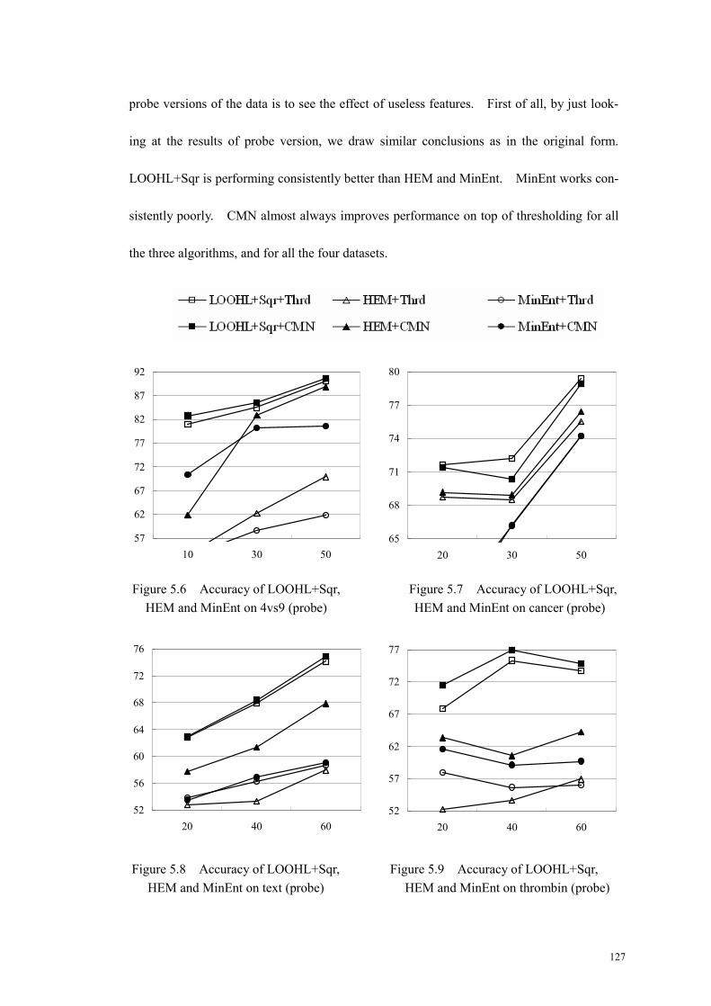
127
probe versions of the data is to see the effect of useless features. First of all, by just look-
ing at the results of probe version, we draw similar conclusions as in the original form.
LOOHL+Sqr is performing consistently better than HEM and MinEnt. MinEnt works con-
sistently poorly. CMN almost always improves performance on top of thresholding for all
the three algorithms, and for all the four datasets.
Figure 5.6 Accuracy of LOOHL+Sqr, HEM and MinEnt on 4vs9 (probe)
Figure 5.7 Accuracy of LOOHL+Sqr, HEM and MinEnt on cancer (probe)
Figure 5.8 Accuracy of LOOHL+Sqr,
HEM and MinEnt on text (probe)
Figure 5.9 Accuracy of LOOHL+Sqr,
HEM and MinEnt on thrombin (probe)
57
62
67
72
77
82
87
92
10 30 5065
68
71
74
77
80
20 30 50
52
56
60
64
68
72
76
20 40 6052
57
62
67
72
77
20 40 60

128
Next, we compare the results on the original version and on the probe version. For cancer
and text dataset probe version outperforms original version, while for 4vs9 and thrombin,
probe version actually underperforms. Since probe version is both performing feature se-
lection by discarding less informative (probably noisy) features and adding new random
features, the real effect of this pre-processing is not very clear. Besides, we downloaded
the probe version directly from NIPS workshop web page, while the original version was
downloaded from other sources. Since the NIPS workshop did not offer the source code
and its description is not in enough detail, it is expected that some fancy pre-processing may
actually improve/hurt the performance of probe version. To be more careful, we
pre-processed the 4vs9 dataset by strictly following the descriptions in NIPS workshop
write-up. However, our probe version dataset yielded significantly different performance
from the probe version directly downloaded. So we are very confident that there must be
some processes omitted in that write-up. Our inability to reproduce the pre-processing
makes the results less conclusive, and the comparison between the performance on original
version and on probe version should be viewed just as reference.
We paid special attention to the probe version of thrombin, and surprisingly CMN does give
improvements there for both LOOHL+Sqr and HEM. This phenomenon does not tally
with our previous argument that the highly unbalanced class distribution should make CMN
behave poorly. We believe that it is not due to our LOOHL+Sqr because HEM is also be-
having in the same way in these two versions. So we may attribute it to the unknown

129
pre-processing in the probe version of thrombin, which made CMN immune to the bad esti-
mation of class distribution.
5.4.2 Comparing four regularizers of LOOHL, under threshold and CMN
In this section, we compare the four regularizers of LOOHL: square loss minimization (Sqr),
eigengap maximization (Eigen), first-hit time minimization regularizer (Step), and row en-
tropy maximization (REnt). The same 9 datasets are used, except the probe form of throm-
bin which is too spatially costly to run in this large scale experiment.
For Eigen, Step and REnt, we enumerated the performance on a grid of the coefficients.
The two coefficients are the initial values of bandwidth σ and the weight ratio between
leave-one-out loss and regularization C1:C2. Since we want to use the result of Sqr in the
previous section as a baseline, we just copied the results in the previous section 5.4 to this
section and did not run on different model coefficients settings. To be fair, we still ran 10
trials using the same labelled examples randomly chosen in section 5.4. In this way, the
Sqr result copied from section 5.4 is comparable with the result of the other regularizers.
The five sub-plots from left to right in the following 8 figures correspond to different values
of σ, common to all datasets. We report here the highest accuracy among all C1:C2, be-
cause reporting the result for each C1:C2 will have to take 24 figures (C1:C2 is discretized to
3 levels). Some points are missing because optimization always failed at the corresponding
coefficient setting. Again, see section B.4 for the details of experimental settings.

130
From the results in Figure 5.10 to Figure 5.17 and the experience of experiment, especially
about C1:C2 which we present in Appendix C, we can draw the following conclusions:
1. The Sqr regularizer with our fixed coefficients generally performs reliably well among
all regularizers. Since the results of Sqr are based on a fixed coefficients and the re-
sults of other regularizers are enumeration of the performance by a number of models
instead of using cross validation model selection, we are quite confident that Sqr is a
reasonable regularizer.
2. The Eigen regularizer yields more promising and more stable accuracy than REnt and
Step. It performs competitively to Sqr regularizer particularly on probe versions. Be-
sides, it is also less prone to numerical problems in optimization.
3. Step regularizer must be used by carefully tuning C1:C2, because unlike Eigen and Rent,
its value is unbounded. It is the regularizer most susceptible to optimization break-
down. As for accuracy, it is not as good as Eigen.
4. The REnt regularizer almost always yields poor accuracy, though its optimization is the
smoothest (i.e., least susceptible to numerical problems) among all the three regulariz-
ers.
5. σ has a more profound influence on both optimization and accuracy than C1:C2. With
larger σ, the optimization can usually proceed more smoothly to the end.
6. When C1:C2 is set in an improper range, the performance can be very poor and numeri-
cal problems are frequently encountered. But when it is set to the proper range, the

131
accuracy is less sensitive to C1:C2 than to σ.
7. CMN is useful for most regularizers, offering improvement on top of thresholding.
8. There still leaves much space to be desired in the direction of regularization. Though
the Eigen, Step, and REnt regularizers seem more theoretically sound than the Sqr regu-
larizer, their empirical performance shows that further research needs to be done into it.

132
71
76
81
86
91
96
10 30 50 10 30 50 10 30 50 10 30 50 10 30 50
σ = 0.15 σ = 0.2 σ = 0.25 σ = 0.3 σ = 0.35
Figure 5.10 Accuracy of four regularizers on 4vs9 (original)
Figure 5.11 Accuracy of four regularizers on cancer (original)
Figure 5.12 Accuracy of four regularizers on text (original)
60
63
66
69
72
75
78
20 30 50 20 30 50 20 30 50 20 30 50 20 30 50
50
55
60
65
70
75
80
20 40 60 20 40 60 20 40 60 20 40 60 20 40 60

133
64
68
72
76
80
84
88
10 20 30 10 20 30 10 20 30 10 20 30 10 20 30
50
56
62
68
74
80
86
20 40 60 20 40 60 20 40 60 20 40 60 20 40 60
Figure 5.13 Accuracy of four regularizers on thrombin (original)
Figure 5.14 Accuracy of four regularizers on ionosphere
Figure 5.15 Accuracy of four regularizers on 4vs9 (probe)
68
73
78
83
88
93
10 30 50 10 30 50 10 30 50 10 30 50 10 30 50

134
62
65
68
71
74
77
80
20 30 50 20 30 50 20 30 50 20 30 50 20 30 50
Figure 5.16 Accuracy of four regularizers on cancer (probe)
Figure 5.17 Accuracy of four regularizers on text (probe)
55
60
65
70
75
80
20 40 60 20 40 60 20 40 60 20 40 60 20 40 60

135
Chapter 6 Conclusions and Future Work
In many practical applications of data classification and data mining, one finds a wealth of
easily available unlabelled examples, while collecting labelled examples can be costly and
time-consuming. In order to make use of the unlabelled data to improve learning perform-
ance, a wide spectrum of semi-supervised learning algorithms have been proposed with pub-
lished success both in theory and in practice. One class of semi-supervised learning algo-
rithm, which is based on graph with nodes representing labelled and unlabelled data and
edges encoding the similarity between data points, has gained particular popularity due to its
natural bridging between supervised learning and unsupervised learning. However, how to
build the underlying graph still has not been well studied, though it is shown to exert sub-
stantial influence on the performance of the learner built upon it.
In this thesis, we presented a graph hyperparameter learning method for graph based
semi-supervised learning. The approach is based on the minimal leave-one-out loss crite-
rion, and an efficient implementation algorithm is designed to overcome the problem of
computational complexity, suffered by most leave-one-out style algorithms. Furthermore,
we investigated the field of graph learning regularization, which is still an unexplored area.
Various regularizers based on graph property, random walk, and spectral clustering are pro-
posed. They help to overcome the problem of learning a degenerative graph by the
leave-one-out loss minimization.

136
However, there are still a lot of open questions and challenges in semi-supervised learning,
and in graph learning in particular. We mention a few below:
1. How to make the optimization more tractable? Although the computational cost is our
central focus and it has already almost reached its lower bound, the optimization proc-
ess can still be very expensive, especially when a large number of iterations are re-
quired or the size of the dataset is large (beyond a few thousand). It might help if an
optimization algorithm is specially designed for this task, rather than using generic op-
timization algorithms (e.g., gradient descent) and packages.
2. How to formulate the problem as a convex optimization problem. Now local minima
are still a problem. However, the matrix inversion operation and the fact that optimi-
zation variables appear in an exponential function make it almost impossible to design a
convex objective function. Is there any other way to define the similarity measure
whose resulting leave-one-out loss function is convex? Or is the/a good graph intrin-
sically not unique?
3. How to deal with structured data, e.g., sequences, trees with all variants? Very recent
work has been done in (Altun et al., 2005) by using maximum margin, graph Laplacian
regularizer and its associated kernel concept in RKHS. Our proposed hyperparameter
learning algorithm assumes that the data points are represented by a numerical vector.
Without such assumption, what is a good parametric form that suits the structured data,

137
and most importantly, keeping the key techniques still applicable which make the
leave-one-out loss minimization efficient and tractable?
4. Is one graph learning algorithm good for all graph based semi-supervised algorithms?
Do different classification algorithm benefit from different graphs? Or do different
tasks, such as clustering, regression, ranking call for graphs designed with different phi-
losophy? Or even for the classification algorithm, does a multi-class task need differ-
ent graphs in applying one-again-rest and one-against-one heuristic?
5. How to incorporate the ideas in kernel learning to graph learning, and vice versa. We
know that there is abundant work on learning the kernels. Since it has been pointed
out that graph Laplacian is closely related to kernels, is it possible to borrow the kernel
learning algorithms to learn a graph, in a form beyond merely learning the spectral
transform?
6. How to design a better graph learning regularizer by making use of reproducing kernel
Hilbert space theory and vice versa. Now even the literature for regularizing learning
the kernels is scarce. However, as we saw in Chapter 4, graph learning provides many
intuitive views on this problem. It will be desirable if such graph properties can be
used to regularize the kernel learning, or in the reverse direction, use the reproducing
kernel Hilbert space theory to design graph learning regularizers.

138
The author hopes that his future doctoral study will lead to the solution of some or most of
these challenges with success.
139
Bibliography
Altun, Yasemin, McAlleste, David and Belkin, Mikhail (2005). Maximum Margin Semi-Supervised Learning for Structured Variables. Neural Information Processing Sys-tems.
Argyriou, Andreas, Herbster, Mark and Pontil, Massimiliano (2005). Combining Graph Laplacians for Semi-Supervised Learning. Neural Information Processing Systems.
Balcan, Maria-Florina, Blum, Avrim and Yang, Ke (2004). Co-Training and Expansion: To-wards Bridging Theory and Practice. Neural Information Processing Systems.
Belkin, Mikhail, Matveeva, Irina and Niyogi, Partha (2004a). Regularization and Semi-supervised Learning on Large Graphs. Conference on Computational Learning The-ory.
Belkin, Mikhail and Nigam, Kamal (2004). Semi-Supervised Learning on Riemannian Manifolds. Machine Learning 56: 209-239.
Belkin, Mikhail, Niyogi, Partha and Sindhwani, Vikas (2004b). Manifold Regularization: A Geometric Framework for Learning from Examples. Technical Report.
Belkin, Mikhail, Niyogi, Partha and Sindhwani, Vikas (2005). On Manifold Regulariza-tion. AI & Statistics.
Bennett, Kristin P. and Demiriz, Ayhan (1998). Semi-Supervised Support Vector Machines. Neural Information Processing Systems.
Benson, Steven J., McInnes, Lois Curfman, Moré, Jorge and Sarich, Jason (2004). TAO User Manual. Manual.
Blum, Avrim and Mitchell, Tom (1998). Combining Labeled and Unlabeled Data with Co-Training. Conference on Computational Learning Theory.
Blum, Avrim and Chawla, Shuchi (2001). Learning from Labeled and Unlabeled Data using Graph Mincuts. International Conference on Machine Learning.
Blum, Avrim, Lafferty, John, Rwebangira, Mugizi Robert and Reddy, Rajashekar (2004). Semi-supervised Learning Using Randomized Mincuts. International Conference on Ma-chine Learning.
Bousquet, Olivier, Chapelle, Olivier and Hein, Matthias (2003). Measure Based Regulariza-tion. Neural Information Processing Systems.
Boyd, Stephen and Vandenberghe, Lieven (2004). Convex Optimization. Cambridge Uni-versity Press.
Boykov, Yuri, Veksler, Olga and Zabih, Ramin (1998). Markov Random Fields with Effi-cient Approximations. IEEE Computer Society Conference on Computer Vision and Pat-

140
tern Recognition.
Carreira-Perpiňán, Miguel Á. and Zemel, Richard S. (2004). Proximity Graphs for Cluster-ing and Manifold Learning. Neural Information Processing Systems.
Castelli, Vittorio and Cover, Thomas M. (1995). On the Exponential Value of Labeled Sam-ples. Pattern Recognition Letters 16(1): 105-111.
Castelli, Vittorio and Cover, Thomas M. (1996). The Relative Value of Labeled and Unla-beled Samples in Pattern Recognition with an Unknown Mixing Parameter. IEEE Transac-tions on Information Theory 42(6): 2102-2117.
Cataltepe, Zehra and Magdon-Ismail, Malik (1998). Incorporating Test Inputs into Learning. Neural Information Processing Systems.
Chapelle, Olivier, Weston, Jason and Schölkopf, Bernhard (2002). Cluster Kernels for Semi-Supervised Learning. Neural Information Processing Systems.
Chapelle, Olivier and Zien, Alexander (2005). Semi-Supervised Classification by Low Den-sity Separation. International Workshop on Artificial Intelligence and Statistics.
Chung, Fan R. K. (1997). Spectral Graph Theory. American Mathematical Society.
Chung, Fan R. K. and Yau, S. T. (2000). Discrete Green's functions. Journal of Combinato-rial Theory (A) 91(1-2): 191-214.
Collins, Michael and Singer, Yoram (1999). Unsupervised Models for Named Entity Classi-fication. Joint SIGDAT Conference on Empirical Methods in Natural Language Process-ing and Very Large Corpora.
Corduneanu, Adrian and Jaakkola, Tommi S. (2001). Stable Mixing of Complete and In-complete Information. Technical Report.
Corduneanu, Adrian and Jaakkola, Tommi (2003). On Information Regularization. Confer-ence on Uncertainty in AI.
Corduneanu, Adrian and Jaakkola, Tommi (2004). Distributed Information Regularization on Graphs. Neural Information Processing Systems.
Cormen, Thomas H., Leiserson, Charles E., Rivest, Ronald L. and Stein, Clifford (2001). Introduction to Algorithms.
Cox, Trevor F. and Cox, Michael A. A. (2001). Multidimensional Scaling. London: Chap-man and Hall.
Crammer, Koby, Keshet, Joseph and Singer, Yoram (2002). Kernel Design Using Boosting. Neural Information Processing Systems.
Cristianini, Nello, Shawe-Taylor, John, Andre, Elisseeff and Kandola, Jaz (2001). On Ker-nel-Target Alignment. Neural Information Processing Systems.
De Bie, Tijl (2005). Semi-supervised Learning Based on Kernel Methods and Graph Cut Algorithms. PhD Thesis.

141
de Silva, Vin and Tenenbaum, Joshua B. (2003). Global versus Local Methods in Nonlinear Dimensionality Reduction. Neural Information Processing Systems.
Doyle, Peter G. and Snell, J. Laurie (1984). Random Walks and Electric Networks. Mathe-matical Association of America.
Fowlkes, Charless, Belongie, Serge, Chung, Fan and Malik, Jitendra (2004). Spectral Grouping Using the Nyström Method. IEEE Transactions on Pattern Analysis and Ma-chine Intelligence 26(2): 214-225.
Freund, Yoav, Seung, H. Sebastian, Shamir, Eli and Tishby, Naftali (1997). Selective Sam-pling Using the Query by Committee Algorithm. Machine Learning 28(2-3): 133-168.
Fung, Glenn and Mangasarian, O. L. (1999). Semi-Supervised Support Vector Machines for Unlabeled Data Classification. Technical Report.
Goldman, Sally and Zhou, Yan (2000). Enhancing Supervised Learning with Unlabeled Data. International Conference on Machine Learning.
Golub, Gene H. and van Loan, Charles F. (1996). Matrix Computations. The Johns Hopkins University Press.
Grady, Leo and Funka-Lea, Gareth (2004). Multi-Label Image Segmentation for Medical Applications Based on Graph-Theoretic Electrical Potentials. European Conference on Computer Vision 2004 Workshop CVAMIA and MMBIA.
Grandvalet, Yves and Bengio, Yoshua (2004). Semi-supervised Learning by Entropy Mini-mization. Neural Information Processing Systems.
Greig, D. M., Porteous, B. and Seheult, A. (1989). Exact Maximum a Posteriori Estimation for Binary Images. Journal of Royal Statistical Society, Series B 51: 271-279.
Grira, Nizar, Crucianu, Michel and Boujemaa, Nozha (2004). Unsupervised and Semi-supervised Clustering: a Brief Survey. Technical Report.
Hagen, Lars and Kahng, Andrew B. (1992). New Spectral Methods for Ratio Cut Partition-ing and Clustering. IEEE Transactions on Computer-Aided Design of Integrated Circuits and Systems 11(9): 1074-1085.
Ham, Jihun, Lee, Daniel D., Mika, Sebastian and Schölkopf, Bernhard (2004). A Kernel View of the Dimensionality Reduction of Manifolds. International Conference on Machine Learning.
Jaakkola, Tommi, Meila, Marina and Jebara, Tony (1999). Maximum Entropy Discrimina-tion. Neural Information Processing Systems.
Joachims, Thorsten (1999). Transductive Inference for Text Classification using Support Vector Machines. International Conference on Machine Learning.
Joachims, Thorsten (2003). Transductive Learning via Spectral Graph Partitioning. Interna-tional Conference on Machine Learning.

142
Jordan, Michael I., Ghahramani, Zoubin, Jaakkola, Tommi S. and Saul, Lawrence K. (1999). An Introduction to Variational Methods for Graphical Models. Machine Learning 37: 183-233.
Jordan, Michael I. (preprint). An Introduction to Probabilistic Graphical Models.
Kapoor, Ashish, Qi, Yuan (Alan), Ahn, Hyungil and Picard, Rosalind W. (2005). Hyper-parameter and Kernel Learning for Graph Based Semi-Supervised Classification. Neural Information Processing Systems.
Kim, Hyun-Chul and Ghahramani, Zoubin (2004). The EM-EP Algorithm for Gaussian Process Classification. European Conference on Machine Learning.
Kleinberg, Jon and Tardos, Eva (1999). Approximation Algorithms for Classification Prob-lems with Pairwise Relationships: Metric Labeling and Markov Random Fields. Sympo-sium on Foundations of Computer Science.
Kohonen, Teuvo (2000). Self-Organizing Maps. Springer.
Kondor, Risi Imre and Lafferty, John (2002). Diffusion Kernels on Graphs and Other Dis-crete Input Spaces. International Conference on Machine Learning.
Kwok, James T. and Tsang, Ivor W. (2003). Learning with Idealized Kernels. International Conference on Machine Learning.
Lanckriet, Gert R. G., Cristianini, Nello, Bartlett, Peter L., Ghaoui, Laurent El and Jordan, Michael I. (2004). Learning the Kernel Matrix with Semidefinite Programming. Journal of Machine Learning Research 5: 27-72.
Lang, Kevin J. (1995). NewsWeeder: Learning to Filter Netnews. International Conference on Machine Learning.
Lee, Wee Sun and Liu, Bing (2003). Learning from Positive and Unlabeled Examples Using Weighted Logistic Regression. International Conference on Machine Learning.
Levin, Anat, Lischinski, Dani and Weiss, Yair (2004). Colorization using Optimization. ACM Transactions on Graphics 23 (3): 689-694.
Li, Wei and McCallum, Andrew (2004). A Note on Semi-Supervised Learning using Markov Random Fields. Technical Report.
Mackay, David J.C. Introduction to Monte Carlo Methods. Tutorial.
Madani, Omid, Pennock, David M. and Flake, Gary W. (2004). Co-Validation: Using Model Disagreement to Validate Classification Algorithms. Neural Information Processing Sys-tems.
Maeireizo, Beatriz, Litman, Diane and Hwa, Rebecca (2004). Co-training for Predicting Emotions with Spoken Dialogue Data. Annual Meeting of the Association for Computa-tional Linguistics.
McCallum, Andrew and Nigam, Kamal Paul (1998). A Comparison of Event Models for
143
Naive Bayes Text Classification. AAAI-98 Workshop on Learning for Text Categorization.
McEliece, Robert J., MacKay, David J. C. and Cheng, Jung-Fu (1998). Turbo Decoding as an Instance of Pearl's `Belief Propagation' Algorithm. IEEE Journal on Selected Areas in Communication 16(2): 140-152.
Meilă, Marina and Shi, Jianbo (2001). A Random Walks View of Spectral Segmentation. AI and Statistics.
Mihalcea, Rada and Chklovski, Timothy (2003). OPEN MIND WORD EXPERT: Creating Large Annotated Data Collections with Web Users' Help. EACL 2003 Workshop on Lin-guistically Annotated Corpora.
Miller, David J. and Uyar, Hasan S. (1996). A Mixture of Experts Classifier with Learning Based on Both Labelled and Unlabelled Data. Neural Information Processing Systems.
Minka, Thomas P. (2001a). A Family of Algorithms for Approximate Bayesian Inference. PhD Thesis, MIT.
Minka, Thomas P. (2001b). Expectation Propagation for Approximate Bayesian Inference. Conference on Uncertainty in AI.
Mitchell, Tom M (1999). The Role of Unlabeled Data in Supervised Learning. International Colloquium on Cognitive Science.
Murphy, Kevin P., Weiss, Yair and Jordan, Michael I. (1999). Loopy Belief Propagation for Approximate Inference: an Empirical Study. Conference on Uncertainty in AI.
Muslea, Ion, Minton, Steve and Knoblock, Craig (2000). Selective Sampling with Redun-dant Views. National Conference on Artificial Intelligence.
Neal, Radford M. (1993). Probabilistic Inference Using Markov Chain Monte Carlo Meth-ods. Tutorial.
Newman, D.J., Hettich, S., Blake, C.L. and Merz, C.J. (1998). UCI Repository of Machine Learning Databases. http://www.ics.uci.edu/~mlearn/MLRepository.html Thesis, Univer-sity of California, Irvine.
Ng, Andrew Y., Jordan, Michael I. and Weiss, Yair (2001a). On Spectral Clustering: Analysis and an Algorithm. Neural Information Processing Systems.
Ng, Andrew Y., Zheng, Alice X. and Jordan, Michael I. (2001b). Link Analysis, Eigenvec-tors and Stability. International Joint Conference on Artificial Intelligence.
Nigam, Kamal, McCallum, Andrew, Thrun, Sebastian and Mitchell, Tom (1999). Text Clas-sification from Labeled and Unlabeled Documents using EM. Machine Learning 39(2/3): 103-134.
Nigam, Kamal Paul and Ghani, Rayid (2000). Analyzing the Effectiveness and Applicability of Co-training. International Conference on Information and Knowledge Management.
Nigam, Kamal Paul (2001). Using Unlabeled Data to Improve Text Classification. PhD The-

144
sis, CMU.
Niu, Zheng Yu, Ji, Dong Hong and Tan, Chew Lim (2005). Word Sense Disambiguation Us-ing Label Propagation Based Semi-Supervised Learning. Annual Meeting of the Associa-tion for Computational Linguistics.
Ong, Cheng Soon and Smola, Alex (2003). Machine Learning using Hyperkernels. Interna-tional Conference on Machine Learning.
Ong, Cheng Soon, Smola, Alexander J. and Williamson, Robert C. (2005). Learning the Kernel with Hyperkernels. Journal of Machine Learning Research 6: 1043-1071.
Opper, Manfred and Winther, Ole (1998). Mean field Methods for Classification with Gaus-sian Processes. Neural Information Processing Systems.
Platt, John (1998). Fast Training of Support Vector Machines using Sequential Minimal Op-timization. Advances in Kernel Methods - Support Vector Learning. B. Schölkopf, C. Burges and A. J. Smola. MIT Press.
Ratsaby, Joel and Venkatesh, Santosh, S. (1995). Learning From a Mixture of Labeled and Unlabeled Examples with Parametric Side Information. Conference on Computational Learning Theory.
Riloff, Ellen and Jones, Rosie (1999). Learning Dictionaries for Information Extraction by Multi-Level Bootstrapping. National Conference on Artificial Intelligence.
Riloff, Ellen, Wiebe, Janyce and Wilson, Theresa (2003). Learning Subjective Nouns using Extraction Pattern Bootstrapping. Conference on Natural Language Learning.
Roweis, Sam and Saul, Lawrence K. (2000). Nonlinear Dimensionality Reduction by Lo-cally Linear Embedding. Science 290(5500): 2323-2326.
Schölkopf, Bernhard and Smola, Alexander J. (2001). Learning with Kernels: Support Vec-tor Machines, Regularization, Optimization, and Beyond. The MIT Press.
Schuurmans, Dale (1997). A New Metric-based Approach to Model Selection. National Conference on Artificial Intelligence.
Schuurmans, Dale and Southey, Finnegan (2000). An Adaptive Regularization Criterion for Supervised Learning. International Conference on Machine Learning.
Seeger, Matthias (2000). Learning with Labeled and Unlabeled Data. Technical Report.
Seung, H., Opper, M. and Sompolinsky, H. (1992). Query by Committee. Annual Workshop on Computational Learning Theory.
Shahshahani, Behzad M. and Landgrebe, David A. (1994). The Effect of Unlabeled Samples in Reducing the Small Sample Size Problem and Mitigating the Hughes Phenomenon. IEEE Transactions on Geoscience and Remote Sensing 18(7): 763-767.
Shi, Jianbo and Malik, Jitendra (2000). Normalized Cuts and Image Segmentation. IEEE Transactions on Pattern Analysis and Machine Intelligence 22(8): 888-905.

145
Smola, Alex and Schölkopf, Bernhard (2003). A Tutorial on Support Vector Regression. Tu-torial.
Smola, Alexander J. and Kondor, Risi Imre (2003). Kernels and Regularization on Graphs. Conference on Computational Learning Theory.
Spielman, Daniel A. and Teng, Shang-Hua (1996). Spectral Partitioning Works: Planar Graphs and Finite Element Meshes. IEEE Symposium on Foundations of Computer Sci-ence.
Stewart, G. W. and Sun, Ji-guang (1990). Matrix Perturbation Theory. Academic Press.
Szummer, Martin and Jaakkola, Tommi (2001). Partially Labeled Classification with Markov Random Walks. Neural Information Processing Systems.
Szummer, Martin and Jaakkola, Tommi (2002). Information Regularization with Partially Labeled Data. Neural Information Processing Systems.
Tenenbaum, Joshua B., de Silva, Vin and Langford, John C. (2000). A Global Geometric Framework for Nonlinear Dimensionality Reduction. Science 290(5500): 2319-2323.
Tikhonov, A. N. (1963). On Solving Incorrectly Posed Problems and Method of Regulariza-tion. Doklady Akademmi Nauk USSR 151: 501-504.
van Rijsbergen, Keith C. J. (1977). A Theoretical Basis for the Use of Co-occurrence Data in Information Retrieval. Journal of Documentation 33(2): 106-119.
Vapnik, Vladimir N. (1998). Statistical Learning Theory. Wiley-Interscience.
Vapnik, Vladimir N. (1999). The Nature of Statistical Learning Theory. Springer.
Wainwright, Martin J. and Jordan, Michael I. (2003). Graphical models, exponential families, and variational inference. Technical Report.
Wainwright, Martin J. and Jordan, Michael I. (2005). A Variational Principle for Graphical Models. New Directions in Statistical Signal Processing. S. Haykin, J. Principe, T. Se-jnowski and J. McWhirter. MIT Press. 21-93.
Watanabe, Satoshi (1969). Knowing and Guessing; a Quantitative Study of Inference and Information. New York, John Wiley and Sons.
Weinberger, Kilian Q. and Saul, Lawrence K. (2004). Unsupervised Learning of Image Manifolds by Semidefinite Programming. IEEE Computer Society Conference on Com-puter Vision and Pattern Recognition.
Weinberger, Kilian Q., Sha, Fei and Saul, Lawrence K. (2004). Learning a Kernel Matrix for Nonlinear Dimensionality Reduction. International conference on Machine learning.
Weinberger, Kilian Q., Packer, Benjamin D. and Saul, Lawrence K. (2005). Nonlinear Di-mensionality Reduction by Semidefinite Programming and Kernel Matrix Factorization. AI & Statistics.
Weiss, Yair (1999). Segmentation using Eigenvectors: a Unifying View. International Con-

146
ference on Computer Vision.
Weston, Jason, Perez-Cruz, Fernando, Bousquet, Olivier, Chapelle, Olivier, Elisseeff, Andre and Schölkopf, Bernhard (2002). Feature Selection and Transduction for Prediction of Molecular Bioactivity for Drug Design.
Yarowsky, David (1995). Unsupervised Word Sense Disambiguation Rivaling Supervised methods. Annual Meeting of the Association for Computational Linguistics.
Yedidia, Jonathan S., Freeman, William T. and Weiss, Yair (2005). Approximations and Generalized Belief Propagation Algorithms. IEEE Transactions on Information Theory 51(7): 2282-2312.
Yu, Stella X., Gross, Ralph and Shi, Jianbo (2002). Concurrent Object Recognition and Segmentation by Graph Partitioning. Neural Information Processing Systems.
Zhang, Tong and Oles, Frank J. (2000). A Probability Analysis on the Value of Unlabeled Data for Classification Problems. International Conference on Machine Learning.
Zhou, Dengyong, Bousquet, Olivier, Lal, Thomas Navin, Weston, Jason and Schölkopf, Bernhard (2003). Learning with Local and Global Consistency. Neural Information Proc-essing Systems.
Zhu, Xiaojin, Ghahramani, Zoubin and Lafferty, John (2003a). Semi-Supervised Learning Using Gaussian Fields and Harmonic Functions. International Conference on Machine Learning.
Zhu, Xiaojin, Lafferty, John and Ghahramani, Zoubin (2003b). Semi-Supervised Learning: From Gaussian Fields to Gaussian Processes. Technical Report.
Zhu, Xiaojin, Lafferty, John and Ghahramani, Zoubin (2003c). Combining Active Learning and Semi-Supervised Learning Using Gaussian Fields and Harmonic Functions. Interna-tional Conference on Machine Learning Workshop.
Zhu, Xiaojin, Kandola, Jaz, Ghahramani, Zoubin and Lafferty, John (2004). Nonparametric Transforms of Graph Kernels for Semi-Supervised Learning. Neural Information Process-ing Systems.
Zhu, Xiaojin (2005). Semi-Supervised Learning with Graphs. PhD Thesis, CMU.
Zhu, Xiaojin and Lafferty, John (2005). Harmonic mixtures: combining mixture models and graph-based methods for inductive and scalable semi-supervised learning. International Conference on Machine Learning.

147
Appendix A Dataset Description and Pre-processing
In this appendix, we describe the datasets used in experiments, their source, property and
how they are pre-processed. As we said before, we were unable to exactly reproduce the
pre-processing according to significant difference in test accuracy. Now we will pay atten-
tion to two questions:
1. How to produce the probe form of the datasets by introducing useless features?
2. What should be the correct original form corresponding to the probe form, i.e., by just
removing the useless features while the other pre-processing steps like helpful feature
selection are still applied?
Some descriptions in this appendix are directly cited from the technical memorandum of
data preparation for NIPS 2003 Workshop on feature selection, which was in turn partly
copied from other sources. We will put all such copied descriptions in quotation mark, and
describe the pre-processing in a way catering for the experiments in this thesis. The NIPS
workshop technical memorandum is downloadable from: http://clopinet.com/isabelle
/Prjects/NIPS2003/Slides/NIPS2003-Datasets.pdf.
A.1. Handwritten digits discrimination: 4 vs 9
The original source of this dataset is MNIST, which is constructed from NIST database.
MNIST is downloadable from http://yann.lecun.com/exdb/mnist/, and it has been very ex-
tensively used as a benchmark dataset. “MNIST size-normalized and centred digits in a

148
0 5 10 15 20 250
5
10
15
20
25
0 5 10 15 20 250
5
10
15
20
25
0 5 10 15 20 250
5
10
15
20
25
0 5 10 15 20 250
5
10
15
20
25
0 5 10 15 20 250
5
10
15
20
25
0 5 10 15 20 250
5
10
15
20
25
fixed size image of dimension 28× 28”, with each pixel having 256 grey levels. On aver-
age, the grey level (feature value) of about 87% pixels is 0. Though MNIST covers digits
from 0 to 9, we are only concerned with distinguishing between 4 and 9. The following
Figure A.1 (a) and (b) are two example images from MNIST.
(a) example of 4 in MNIST (b) example of 9 in MNIST
(c) example of 4 after thresholding (d) example of 9 after thresholding
(e) average of 4 in the whole MNIST (f) average of 9 in the whole MNIST
Figure A.1 Image examples of handwritten digit recognition

149
The size of the original dataset is very large. Combining training and testing set, there are
70,000 examples in all for the 10 classes. Each example is a vector with 784 components,
varying from 0 to 255 in discrete values. So storing them in a binary file using 32-bit inte-
ger will cost over 400 MB. The data file was compressed in a special format to 54 MB.
We used the Matlab program written by Bryan Russell and Kevin Murphy to parse the com-
pressed file: http://www.cs.ubc.ca/~murphyk/Software/readMNIST.m. We randomly ex-
tracted 1000 examples for ‘4’ and ‘9’ each, which formed digitOri.dat1. We only applied
five simple preprocess steps here as detailed in genDigitOri.cpp. Suppose the columns are
features and the rows are examples.
1. Among the 784 original features, eliminate all the features which have only zero values
or constant values;
2. Standardize by linearly transforming each feature (each column) so that the values in
each column would be in the range [0,1] ;
3. “Threshold values below 0.5 to increase data sparsity” (after this step the examples of
Figure A.1 (a) and (b) become (c) and (d) respectively);
4. Discard all the features which appear (nonzero) for less than 3 times;
5. Normalize each example (in each row) so that the length of feature vector is 1 for all
examples.
------------------------------------------
Now we get the so-called “original version” of the data in the experiment.
1 As we redid the pre-processing for 4 vs 9 dataset, we put the processing code and resulting dataset online and we mention the file names in this section.
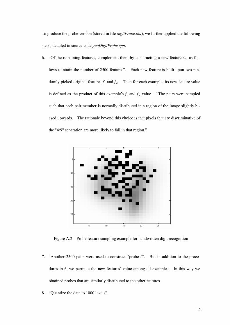
150
To produce the probe version (stored in file digitProbe.dat), we further applied the following
steps, detailed in source code genDigitProbe.cpp.
6. “Of the remaining features, complement them by constructing a new feature set as fol-
lows to attain the number of 2500 features”. Each new feature is built upon two ran-
domly picked original features f 1 and f 2. Then for each example, its new feature value
is defined as the product of this example’s f 1 and f 2 value. “The pairs were sampled
such that each pair member is normally distributed in a region of the image slightly bi-
ased upwards. The rationale beyond this choice is that pixels that are discriminative of
the "4/9" separation are more likely to fall in that region.”
Figure A.2 Probe feature sampling example for handwritten digit recognition
7. “Another 2500 pairs were used to construct "probes"”. But in addition to the proce-
dures in 6, we permute the new features’ value among all examples. In this way we
obtained probes that are similarly distributed to the other features.
8. “Quantize the data to 1000 levels”.
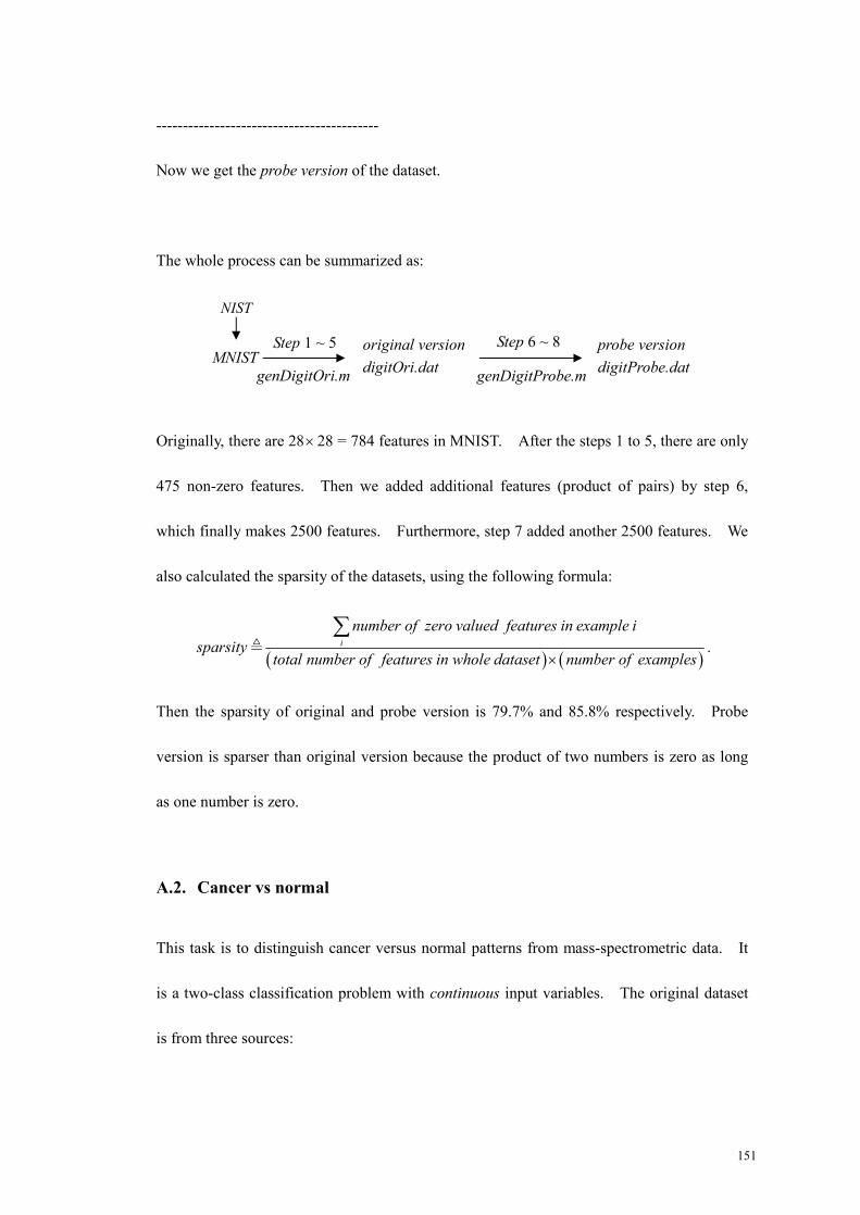
151
------------------------------------------
Now we get the probe version of the dataset.
The whole process can be summarized as:
Originally, there are 28× 28 = 784 features in MNIST. After the steps 1 to 5, there are only
475 non-zero features. Then we added additional features (product of pairs) by step 6,
which finally makes 2500 features. Furthermore, step 7 added another 2500 features. We
also calculated the sparsity of the datasets, using the following formula:
( ) ( )i
number of zero valued features in example isparsity
total number of features in whole dataset number of examples×
∑ .
Then the sparsity of original and probe version is 79.7% and 85.8% respectively. Probe
version is sparser than original version because the product of two numbers is zero as long
as one number is zero.
A.2. Cancer vs normal
This task is to distinguish cancer versus normal patterns from mass-spectrometric data. It
is a two-class classification problem with continuous input variables. The original dataset
is from three sources:
MNIST original version digitOri.dat
Step 1 ~ 5 probe version digitProbe.dat
Step 6 ~ 8
NIST
genDigitOri.m
genDigitProbe.m

152
download URL No. of
spectra
No. of can-
cer spectra
No. of con-
trol spectra
No. of
features
NCI ovarian
data
http://home.ccr.can
cer.gov/ncifdaprote
omics/ppatterns.asp
253 162 91
15154
continuously
valued
NCI prostate
cancer data
http://home.ccr.can
cer.gov/ncifdaprote
omics/ppatterns.asp
322 69 253
15154
continuously
valued
EVMS pros-
tate cancer
data
http://www.evms.e
du/vpc/seldi/ 326 167 159
48538
continuously
valued
Table A.1 Cancer dataset summary
Merging the three sources, we obtain a dataset of mass-spectra obtained with the SELDI
technique. The samples include patients with cancer (ovarian or prostate cancer), and
healthy (or control) patients. The total number of examples is 253+322+326 = 901, among
which 162+69+167 = 398 examples are cancer samples (positive class) and 91+253+159 =
503 are control samples (negative class). It is interesting to put the two kinds of cancer
together. Due to lack of domain knowledge, we did not redo the pre-processing and we
describe how the probe version was produced by the NIPS workshop. All examples were
merged at first, by adding 48538 and 15154 zero-valued features to NCI and EVMS exam-
ples respectively. Then 9 simple pre-processing steps were applied. Suppose the columns

153
are features and the rows are examples (the 9 steps below are all cited from NIPS workshop).
1. “Limit the mass range. Eliminate small masses under m/z=200 that usually include
chemical noise specific to the MALDI/SELDI process (influence of the “matrix”).
Also eliminate large masses over m/z = 10000 because few features are usually relevant
in that domain and we needed to compress the data.
2. Average the technical repeats. In the EVMS data, two technical repeats were available.
They were averaged in order to make examples in the test set independent so that sim-
ple statistical tests could be applied.
3. Remove the baseline. Subtract in a window the median of the 20% smallest values.
4. Smoothing. The spectra were slightly smoothed with an exponential kernel in a win-
dow of size 9.
5. Re-scaling. The spectra were divided by the median of the 5% top values.
6. Take the square root of all feature values.
7. Align the spectra. Slightly shift the spectra collections of the three datasets so that the
peaks of the average spectrum would be better aligned. As a result, the mass-over-
charge (m/z) values that identify the features in the aligned data were imprecise. The
NCI prostate cancer m/z was taken as reference.
8. Soft thresholding the values. After examining the distribution of values in the data
matrix, we subtracted a threshold and equaled to zero all the resulting values that were
negative. In this way, only about 50% of non-zero values were kept, which repre-
sented significant data compression.
9. Quantization. Quantize the values to 1000 levels.”

154
------------------------------------------
Now we get the so-called “original version” of the data in the experiment.
To produce the probe version, we apply the following processing:
10. “Identify the region of the spectra with least information content using an interval search
for the region that gave worst prediction performance of a linear SVM (indices
2250-4750). The features in that region were replaced by “random probes” obtained by
randomly permuting the values in the columns of the data matrix.
11. Identify another region of low information content: 6500-7000, and then add 500 random
probes that are permutations of those features.”
------------------------------------------
Now we get the probe version of the dataset.
A.3. Reuters text categorization: "corporate acquisitions" or not
This task is to classify whether a text is about "corporate acquisitions" or not. This is a
two-class classification problem with sparse continuous input variables.
The original source of the dataset is the well-known Reuters text categorization benchmark,
hosted at http://kdd.ics.uci.edu/databases/reuters21578/reuters21578.html. Another valuable
source about this data is http://www.daviddlewis.com/resources/testcollections/reuters21578/.
We used a subset of it: the “corporate acquisition” text classification class pre-processed by
Thorsten Joachims. As one of the examples of the software SVMlight, it is downloadable

155
from http://download.joachims.org/svm_light/examples/example1.tar.gz.
“The data formatted by Joachims is in the "bag-of-words" representation. There are 9947
features (of which 2562 are always zero for all the examples) that represent frequencies of
occurrence of word stems in text. Some normalization has been applied that are not de-
tailed by Joachims in his documentation.” We randomly extracted 2000 examples (class
balanced) which formed the original version. The only pre-processing applied on top of
Joachims’ data is to discard all the features which appear (nonzero) for less than 3 times.
“The frequency of appearance of words in text is known to follow approximately Zipf’s law
(for details, see e.g. http://www.nslij-genetics.org/wli/zipf/). According to that law, the fre-
quency of occurrence of words, as a function of the rank k when the rank is determined by
the frequency of occurrence, is a power-law function Pk ~ k – a with the exponent a close to 1.
The estimation a = 0.9 gives us a reasonable approximation of the distribution of the data.”
Figure A.3 Comparison of the real data and the random probe data distributions

156
Figure A.3 plots the number of non-zero values of a given feature as a function of the rank of
the feature. The rank is given by the number of non-zero features. Red: real data. Blue:
simulated data.
To produce the probe version, the following pre-processing steps were applied:
1. “Add to the original 9947 features, 10053 features drawn at random according to Zipf’s
law, to obtain a total of 20000 features. Fraction of non-zero values in the real data is
0.46% while fraction of non-zero values in the simulated data: 0.5%.
2. The feature values were quantized to 1000 levels.”
------------------------------------------
Now we get the probe version of the dataset.
A.4. Compounds binding to Thrombin
This task is to predict which compounds bind to thrombin. It is a two-class classification
problem with sparse binary input variables.
“Drugs are typically small organic molecules that achieve their desired activity by binding to
a target site on a receptor. The first step in the discovery of a new drug is usually to identify
and isolate the receptor to which it should bind, followed by testing many small molecules for
their ability to bind to the target site. This leaves researchers with the task of determining
what separates the active (binding) compounds from the inactive (nonbinding) ones. Such a
determination can then be used in the design of new compounds that not only bind, but also

157
have all the other properties required for a drug (solubility, oral absorption, lack of side ef-
fects, appropriate duration of action, toxicity, etc.). Biological activity in general, and re-
ceptor binding affinity in particular, correlate with various structural and physical properties
of small organic molecules. In this task, we are concerned with compounds’ ability to bind
to a target site on thrombin, a key receptor in blood clotting.
The original combined dataset consisted of 2543 compounds, of which 192 are active (bind
well) and the others (2351) are inactive. To simulate the real-world drug design environ-
ment, the test set contained 634 compounds that were in fact generated based on the assay
results recorded for the training set (1909 compounds). Of the test compounds, 150 bind
well and the others are inactive. The compounds in the test set were made after chemists
saw the activity results for the training set, so the test set had a higher fraction of actives
than did the training set in the original data split. In evaluating the accuracy, a differential
cost model was used, so that the sum of the costs of the actives will be equal to the sum of
the costs of the inactive.
Each compound is described by a single feature vector comprised of 139,351 binary features,
which describe three-dimensional properties of the molecule. The chemical structures of
these compounds are not necessary for our analysis. On average, less than 1% feature val-
ues are non-zero. The original source of the data is from KDD Cup 2001:
http://www.cs.wisc.edu/~dpage/kddcup2001.”

158
All the examples from the original source KDD Cup were used and 5 pre-processing steps
were applied.
1. To capitalize on the differences in the distribution between the training and test dataset, a
technique in (Weston et al., 2002) was adopted. For all features f j, compute a score
: 1 : 1i ij ij iji y i y
f X Xλ= =−
= −∑ ∑
where the matrix X is the testing dataset, with columns being features and rows being
examples. “The features were sorted according to the f j criterion with λ = 3, computed
using the original test set, which is richer in positive (active) examples.”
2. “Only the top ranking 100,000 original features were kept.”
3. Discard all the remaining features which appear (nonzero) for less than 3 times.
4. “The all-zero patterns were removed, except one that was given label –1 (inactive).”
------------------------------------------
Now we get the so-called “original version” of the data in the experiment.
To produce the probe version, the following pre-processing step was applied:
5. “For the second half lowest ranked features, the order of the patterns was individually
randomly permuted, in order to create “random probes”. So now half of the features
are real original features while the other half are probe features.”
------------------------------------------
Now we get the probe version of the dataset.
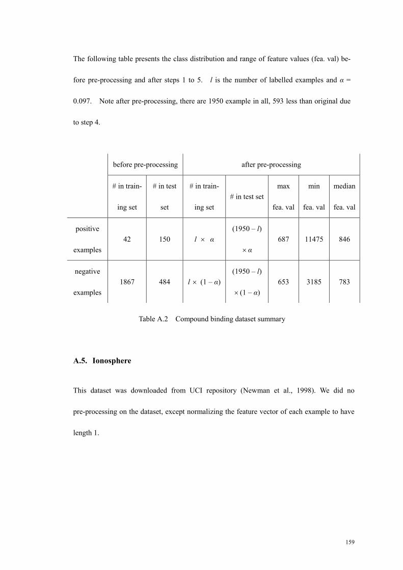
159
The following table presents the class distribution and range of feature values (fea. val) be-
fore pre-processing and after steps 1 to 5. l is the number of labelled examples and α =
0.097. Note after pre-processing, there are 1950 example in all, 593 less than original due
to step 4.
before pre-processing after pre-processing
# in train-
ing set
# in test
set
# in train-
ing set # in test set
max
fea. val
min
fea. val
median
fea. val
positive
examples 42 150 l × α
(1950 – l)
× α 687 11475 846
negative
examples 1867 484 l × (1 – α)
(1950 – l)
× (1 – α) 653 3185 783
Table A.2 Compound binding dataset summary
A.5. Ionosphere
This dataset was downloaded from UCI repository (Newman et al., 1998). We did no
pre-processing on the dataset, except normalizing the feature vector of each example to have
length 1.

160
Appendix B Details of Experiment Settings
In this appendix, we present miscellaneous details of experiments, including algorithm im-
plementation, dataset choosing, cross validation, and experimental settings.
B.1. Toolboxes used for learning algorithm implementation
All the 12 algorithms were implemented by the author in C++, mixing two toolboxes:
1. Matlab C++ Math library for four matrix operations: matrix multiplication, matrix
power, matrix inversion and matrix eigen-decomposition. Matlab offers almost the
most efficient implementation of these operations. In particular, it has reduced the cost
of full matrix inversion to be far below ( )3O u . The detail of its implementation is not
released by Mathworks.
2. Toolkit for Advanced Optimization (TAO) by (Benson et al., 2004) for gradient descent
optimization in all the algorithms compared except HEM. This package implements
three variations of conjugate gradient methods: the Fletcher-Reeves method, the Po-
lak-Ribiére method, and Polak-Ribiére-Plus method. It also implemented a limited
memory variable metric method (lmvm) for unconstrained nonlinear optimization that
requires only function value and gradient information. It keeps a limited history of pre-
vious points and previous gradients to approximate the second-order information. We
use lmvm for all optimizations.
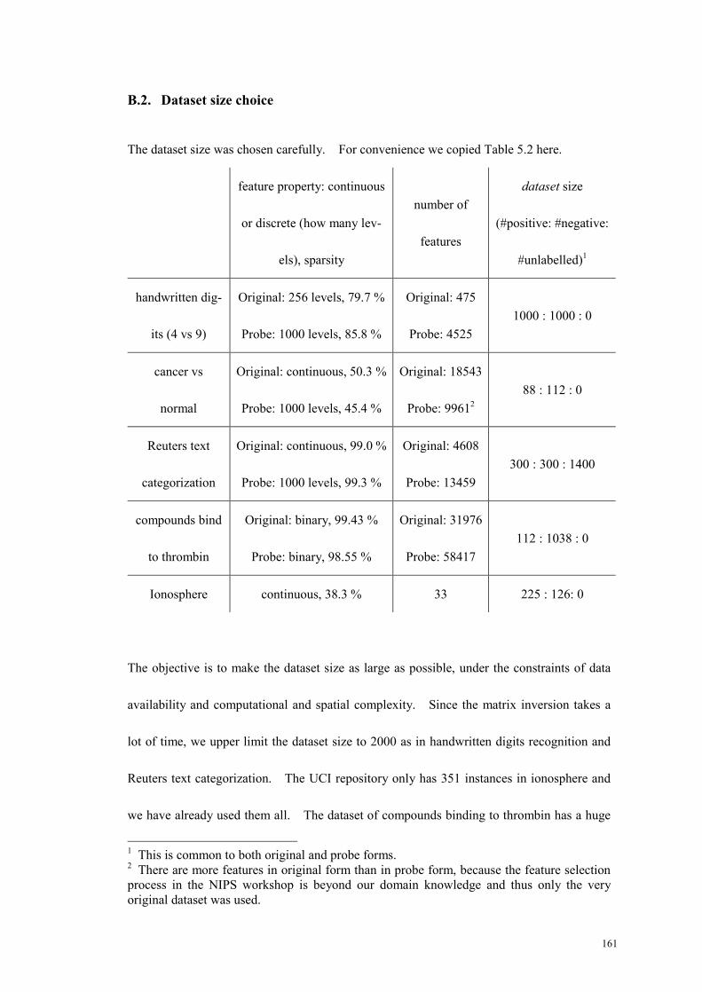
161
B.2. Dataset size choice
The dataset size was chosen carefully. For convenience we copied Table 5.2 here.
feature property: continuous
or discrete (how many lev-
els), sparsity
number of
features
dataset size
(#positive: #negative:
#unlabelled)1
handwritten dig-
its (4 vs 9)
Original: 256 levels, 79.7 %
Probe: 1000 levels, 85.8 %
Original: 475
Probe: 4525 1000 : 1000 : 0
cancer vs
normal
Original: continuous, 50.3 %
Probe: 1000 levels, 45.4 %
Original: 18543
Probe: 99612 88 : 112 : 0
Reuters text
categorization
Original: continuous, 99.0 %
Probe: 1000 levels, 99.3 %
Original: 4608
Probe: 13459 300 : 300 : 1400
compounds bind
to thrombin
Original: binary, 99.43 %
Probe: binary, 98.55 %
Original: 31976
Probe: 58417 112 : 1038 : 0
Ionosphere continuous, 38.3 % 33 225 : 126: 0
The objective is to make the dataset size as large as possible, under the constraints of data
availability and computational and spatial complexity. Since the matrix inversion takes a
lot of time, we upper limit the dataset size to 2000 as in handwritten digits recognition and
Reuters text categorization. The UCI repository only has 351 instances in ionosphere and
we have already used them all. The dataset of compounds binding to thrombin has a huge
1 This is common to both original and probe forms. 2 There are more features in original form than in probe form, because the feature selection process in the NIPS workshop is beyond our domain knowledge and thus only the very original dataset was used.

162
number of features in the probe form. Since the probe form is directly downloaded from
web site, we do not know the detailed meanings of each number. So we keep all features.
That makes the spatial cost huge: over 2.2 GB memory used for 1200 examples in our
LOOHL implementation. So we stop at 1200. The number of features in cancer (origin)
is only around 1/1.6 of thrombin (origin). However, the cancer dataset has a significantly
lower sparsity (50.3/45.4 vs 99.43/98.55). So we used a small dataset size.
B.3. Cross validation complexity analysis
The unit of cross validation complexity analysis is the process denoted by the shorthand:
Score( , , , , , ,l l ute teX Y X Y X A λ )
For example, in the HEM algorithm, A stands for HEM and λ stands for the coefficients
such as the bandwidth of the similarity measure. Now suppose we have 10 labelled articles
( ),l lX Y = ( )1...10 1...10,X Y and 80 unlabelled articles ( )11...90uX X= . Besides we are given
other 10 testing articles ( )91...100teX X= and we wish to compare the prediction of the algo-
rithm against the correct labels of these 10 testing articles ( )91...100teY Y= . As the HEM al-
gorithm is transductive, we can get the model’s labelling on teX directly by learning from
the 100 articles in whole. However, we can also use A = TSVM, λ = type of kernel,
RBF kernel bandwidth, C (trade-off factor between loss and margin), fraction of unlabelled
examples to be classified into the positive class. Different from HEM, TSVM can pro-
duce an inductive model, i.e., we can get a model M: ( ) ( ),i i iif x y k x xα= ∑ by learning
from , , ,l l uteX Y X X . Then we simply feed teX to M and compare the prediction against
teY . By using the notation Score( , , , , , ,l l ute teX Y X Y X A λ ), we can treat transductive and
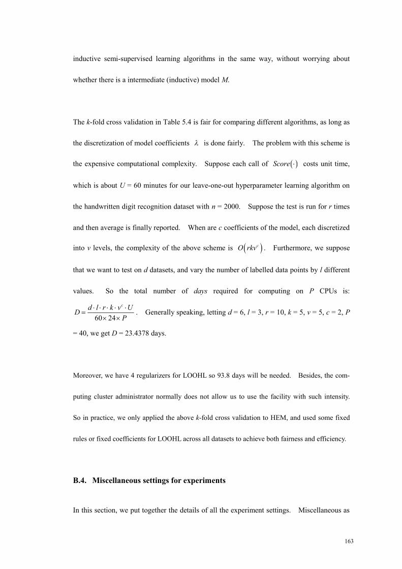
163
inductive semi-supervised learning algorithms in the same way, without worrying about
whether there is a intermediate (inductive) model M.
The k-fold cross validation in Table 5.4 is fair for comparing different algorithms, as long as
the discretization of model coefficients λ is done fairly. The problem with this scheme is
the expensive computational complexity. Suppose each call of ( )Score ⋅ costs unit time,
which is about U = 60 minutes for our leave-one-out hyperparameter learning algorithm on
the handwritten digit recognition dataset with n = 2000. Suppose the test is run for r times
and then average is finally reported. When are c coefficients of the model, each discretized
into v levels, the complexity of the above scheme is ( )cO rkv . Furthermore, we suppose
that we want to test on d datasets, and vary the number of labelled data points by l different
values. So the total number of days required for computing on P CPUs is:
60 24
cd l r k v UDP
⋅ ⋅ ⋅ ⋅ ⋅=
× ×. Generally speaking, letting d = 6, l = 3, r = 10, k = 5, v = 5, c = 2, P
= 40, we get D = 23.4378 days.
Moreover, we have 4 regularizers for LOOHL so 93.8 days will be needed. Besides, the com-
puting cluster administrator normally does not allow us to use the facility with such intensity.
So in practice, we only applied the above k-fold cross validation to HEM, and used some fixed
rules or fixed coefficients for LOOHL across all datasets to achieve both fairness and efficiency.
B.4. Miscellaneous settings for experiments
In this section, we put together the details of all the experiment settings. Miscellaneous as

164
it is, we will try to organize them as clearly as possible. The experiments are random in
nature. However in order to make the experiments totally reproducible, we have stored all
the source programs (both for pre-processing and for learning algorithm implementation),
data files (raw data with and without probe features), main control files (scripts), and seed of
random number generator. All these files and seeds are available at http://www.comp.nus.
edu.sg/~zhangxi2/thesis.html. A short manual is also written to accompany the programs.
The raw results and the performance under different coefficients during cross validation
model selection are also available on the web site.
The experiments were divided into two parts of comparisons:
1. Compare the performance of HEM, MinEnt, and LOOHL+sqr, each with both threshold
form and CMN form, on the same 4 2 1 9× + = datasets by using 5 fold cross validation
as model selection, or by fixing the value of coefficients across all datasets;
2. Compare the four regularizers of LOOHL on the same 9 datasets by enumerating the
accuracy under a number of coefficient values without model selection.
We will refer to these two parts as part 1 and part 2.
1. Data pre-processing. The details of data pre-processing is in the Appendix A. We
just emphasize that all the input feature vectors were normalized to have length 1. Be-
fore that, all features which appear (non-zero) in less than three instances in the whole
dataset were filtered out. This will help compress data because in many datasets, espe-
cially text dataset according to Zipf’s law, such infrequently appearing features consti-
tute a large bulk of the total features. This pruning also helps to avoid overfitting,

165
similar to avoiding such rules as (birth date → score) in decision tree learning.
2. Model selection. In part 1, we used 5 fold cross validation to select the model for
HEM. For MinEnt, we tested the accuracy on all the discretized coefficients and then
report the highest accuracy without cross validation, which is an unfair advantage for
MinEnt. The only exceptions are cancer and ionosphere, for which we used 5 fold
cross validation as well since the computational cost is mild on these two datasets.
For LOOHL+Sqr, we chose the prior mean of the bandwidth in the regularizer as the
bandwidth selected by HEM+Thrd via cross validation. This value also served as the
initial value for iterative optimization in LOOHL+Sqr. Once it caused numerical
problems in optimization, e.g., line search failure, not-a-number or infinity due to in-
verting a matrix close to singular, etc., we just increased the bandwidth (both the prior
mean and the initial value) by 0.05, until the graph was connected strongly enough and
there was no numerical problem in the optimization process. All other coefficients
were fixed across all datasets as detailed in point 4 below. In practice, we found that
the resulting accuracy was always reasonable when the optimization proceeded
smoothly, i.e., no numerical problems occurred.
In part 2, we present the performance by enumerating all the coefficients on a chosen
grid, without doing model selection via cross validation. This is because the LOOHL+
regularizers is very time consuming and requires a lot of computing recourses. We
have already shown the performance of regularizer Sqr in part 1, by fixing all the coeffi-

166
cient values and thus on a fair basis of comparison. So in part 2, we aim at showing the
promise of the other three regularizers, and it will also provide some insight into the
good choices of coefficients.
3. Cross validation was applied only in part 1 for HEM (all datasets) and MinEnt (cancer
and ionosphere). We used 5 fold cross validation. As the input vectors were all nor-
malized, we could fix the grid/discretization for candidate models in HEM across all
datasets. The candidate σ’s are 0.05, 0.1, 0.15, 0.2, 0.25. MinEnt also used these five
σ’s as initial values for gradient descent, while its candidate ε’s are 0.01, 0.05, 0.1, 0.2,
0.3. We ran some initial experiments and found that the models picked for HEM and
MinEnt are almost always in the interior of this grid and the step is refined enough.
4. Fixed coefficients. For all LOOHL algorithms in both parts, we fixed ε to 0.01. The
LOO loss transformation function was fixed to the polynomial form with exponent 3 (ref.
Figure 3.2), and the eigenvalue penalty exponent was fixed to 3 as well (ref. (4.1)).
The prior q in CMN (2.7) was always set to the class ratio in training set, except for the
thrombin dataset as detailed in the below point 5.
In part 1, if the objective is written as C1 * LOO_loss + C2 * regularizer, then we fixed
C1:C2 to 100:1 for LOOHL+Sqr across all datasets. In part 2, we will show the influ-
ence of different C1:C2 and different bandwidth σ under the other three regularizers.
C1:C2 are chosen to be 1:10, 1:100, and 1:1000 for all the datasets on regularizers Eigen

167
and REnt. This is because the value of these two regularizers is bounded by a constant.
However, as the first-hit time is not bounded, we carefully chose some candidate C1:C2
values for Step regularizer so that the optimization could proceed properly. For 4vs9,
cancer and ionosphere, we chose 1:10, 1:100, 1:1000. For text and thrombin, we chose
1:1000, 1:104, 1:105. The absolute values of C1 and C2 will be discussed in point 6.
5. Performance measure. We used accuracy as performance measure on all datasets ex-
cept thrombin binding, where the two classes are very unbalanced at about 1:10. In the
NIPS workshop, the balanced error rate (BER) was used: 12
b cBERa b c d
+ + + ,
where
prediction number of examples
in test set positive negative
positive r+ a b truth
negative r– c d
This is equivalent to super-sampling the truly positive examples by (c+d) times, and su-
per-sampling the truly negative examples by (a+b) times. We used 1 – BER as our
balanced accuracy for thrombin binding dataset. The whole learning algorithm of
HEM and LOOHL did not change. However, we gave some advantage to HEM+
CMN for thrombin dataset, by allowing it to know the correct class distribution in the
test set. Suppose in labelled data, there are r+ positive instances and r– negative in-
stances. Then previously we set ( )1q r r r+ + −= + . Now given that we know there are

168
s+ positive instances and s– negative instances in the test set, we set ( )2q s s s+ + −= + ,
the correct proportion. However, the weighted cost elicited some other considerations.
If : 1:10s s+ − = , then by the definition of BER, the loss of misclassifying a truly posi-
tive point into negative will be 10 times as much as the opposite misclassification. So
we may prefer to be conservative and be more willing to bias the prediction towards the
positive class, i.e., avoid making costly mistakes, by setting ( )3q s s s− + −= + . In
HEM+CMN for thrombin dataset, we will report the average of the highest accuracy for
each test point among using q1, q2 and q3.
6. Optimization configurations. We always used the lmvm algorithm to perform gradient
descent for LOOHL with various regularizers. Although σ appears only in the form of
σ 2, we still used σ as optimization variable because otherwise if we use 2α σ as vari-
able, we will have to add a constraint 0α ≥ , and constrained programming is usually
more complicated than unconstrained programming. Although optimizing over σ will
result in multiple optimal solutions, the optimization problem is non-convex by itself,
and the gradient descent will just find a local minimum. Empirically, we noticed that
the local minimum found by the solver is usually close to the initial value.
Although the absolute value of C1 and C2 in above point 3 does not influence the optimal
variable value in theory, the solver of the optimization toolkit is sensitive to the absolute
value in practice. So we picked C1 and C2 according to the behaviour of the solver,
tuning it among 10n (where n is an integer), so that it will proceed properly without

169
looking at the test accuracy. Poorly chosen C1 and C2 will quickly cause numerical
problems in optimization. We chose C1 = 10000 for 4vs9 and cancer datasets, C1 = 100
for text and thrombin binding, and C1 = 1000 for ionosphere. For each dataset, the
same C1 applied to both part 1 and part 2 of the experiment.
In part 1, the initial value of σ for gradient descent in LOOHL+Sqr was chosen as the 5
fold cross validation result of HEM+Thrd, and then increased by 0.05 until no numerical
problem occurs (as detailed in point 2). The initial values of σ for MinEnt were 0.05,
0.1, 0.15, 0.2, and 0.25. In part 2, the initial values of σ chosen were 0.15, 0.2, 0.25,
0.3, and 0.35. Different from Sqr which also used the initial σ as prior mean, the other
three regularizers only used it as an initial value for optimization.
Finally we limited the number of function evaluation to 35 on all datasets except iono-
sphere. This was to avoid the situations of extremely slow convergence. In most of
the time, lmvm converged in 35 times of function evaluation (not 35 iterations because
the number of function evaluation in each iteration is not fixed). We will also report
the result under this cut-off optimization because usually this is believed to occur at
some flat region and it is still believed to be a reasonable value.
7. Platform consideration. How to make full use of the computing resources is also an
important problem in practice. We summarize the software and hardware configura-
tions of the computing facilities we have access to.

170
CPU number, type
and frequency bit
memory (GB)
Matlab run-time library available?
node type
access0-13 2× P4 2.8GHz 32 2.5 √ access (interactive)
sma0-14 4× Opteron 2.2GHz 64 2.0 × access (interactive)
comp0-41 2× P4 2.8GHz 32 1.01 √ compute (batch)
compsma0-34 2× Opteron 2.2GHz 64 2.0 × compute (batch)
Table B.1 Hardware and software configurations of computing cluster
On none of the above nodes can we compile Matlab code. We compiled Matlab code on
twinkle.ddns.comp.nus.edu.sg, which is a 32-bit machine. Then we transferred the execu-
table to the 32-bit compute cluster nodes. Let us also consider the four other algorithms
mentioned Table 5.1. Implementation of SVM/TSVM is available at http://svmlight.
joachims.org/, written in pure C. We have implemented st-mincut in pure C++ by making
use of the max flow implementation by Yuri Boykov and Vladimir Kolmogorov
(http://www.cs.cornell.edu/People/vnk/software.html). SGT is available at http://sgt.
joachims.org/, which uses Matlab Math library for matrix inversion and eigen
-decomposition just like HEM, MinEnt, and LOOHL. In sum, we can dispatch jobs in the
following way:
LOOHL HEM MinEnt SGT SVM/TSVM st-mincut
access0-13 comp0-41 compsma0-34 or comp0-41
1 It is relatively small, especially under the multi-user environment.

171
Appendix C Detailed Result of Regularizers
In this appendix, we give the detailed results of the regularizers for LOOHL when enumer-
ating on the grid of σ (initial bandwidth for optimization) and C1:C2. For Eigen, Step and
REnt, the initial values of σ chosen were 0.15, 0.2, 0.25, 0.3, and 0.35, which correspond to
the five sub-plots from left to right in the following 24 figures. C1:C2 were chosen to be
1:10, 1:100, and 1:1000 for all the datasets on Eigen and REnt regularizers. As for Step
regularizer, we chose 1:10, 1:100, 1:1000 for 4vs9, cancer and ionosphere, and chose 1:103,
1:104, 1:105 for text and thrombin (ref. point 4 and 6 in appendix section B.4). We will call
these C1:C2 as rmax, rmedium, rmin respectively in a uniform way across all datasets, i.e. rmax =
1:10 for cancer while rmax = 1:103 for text. The x-axis stands for the number of labelled
points and the y-axis stands for accuracy (balanced accuracy for thrombin). Some points
are missing because optimization always failed at the corresponding coefficient setting.

172
48535863687378838893
10 20 30 10 20 30 10 20 30 10 20 30 10 20 30
rowEnt+Thrd rowEnt+CMN step+Thrd step+CMN
eigen+Thrd eigen+CMN sqr+Thrd sqr+CMN
σ = 0.15 σ = 0.2 σ = 0.25 σ = 0.3 σ = 0.35
Figure C.1 Accuracy of four regularizers on 4vs9 (original) under rmax The Step regularizer met numerical problems in optimization for all σ under this C1:C2.
Figure C.2 Accuracy of four regularizers on 4vs9 (original) under rmedium
Figure C.3 Accuracy of four regularizers on 4vs9 (original) under rmin
61
66
71
76
81
86
91
96
10 20 30 10 20 30 10 20 30 10 20 30 10 20 30
65
70
75
80
85
90
95
10 20 30 10 20 30 10 20 30 10 20 30 10 20 30
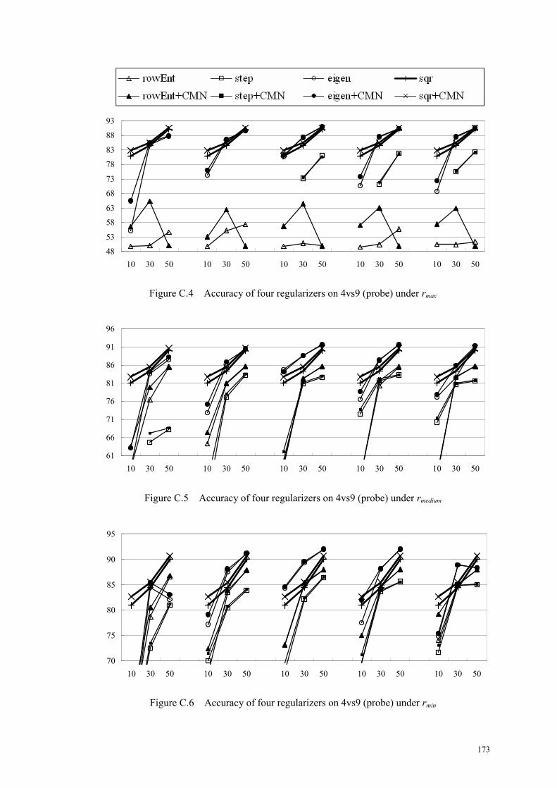
173
48
53
58
63
68
73
78
83
88
93
10 30 50 10 30 50 10 30 50 10 30 50 10 30 50
rowEnt+Thrd rowEnt+CMN step+Thrd step+CMN
eigen+Thrd eigen+CMN sqr+Thrd sqr+CMN
Figure C.4 Accuracy of four regularizers on 4vs9 (probe) under rmax
Figure C.5 Accuracy of four regularizers on 4vs9 (probe) under rmedium
Figure C.6 Accuracy of four regularizers on 4vs9 (probe) under rmin
61
66
71
76
81
86
91
96
10 30 50 10 30 50 10 30 50 10 30 50 10 30 50
70
75
80
85
90
95
10 30 50 10 30 50 10 30 50 10 30 50 10 30 50

174
48
53
58
63
68
73
20 30 50 20 30 50 20 30 50 20 30 50 20 30 50
rowEnt+Thrd rowEnt+CMN step+Thrd step+CMN
eigen+Thrd eigen+CMN sqr+Thrd sqr+CMN
60
63
66
69
72
75
78
20 30 50 20 30 50 20 30 50 20 30 50 20 30 50
61
64
67
70
73
76
20 30 50 20 30 50 20 30 50 20 30 50 20 30 50
Figure C.7 Accuracy of four regularizers on cancer (original) under rmax
Figure C.8 Accuracy of four regularizers on cancer (original) under rmedium
Figure C.9 Accuracy of four regularizers on cancer (original) under rmin

175
48
56
64
72
80
20 30 50 20 30 50 20 30 50 20 30 50 20 30 50
rowEnt+Thrd rowEnt+CMN step+Thrd step+CMN
eigen+Thrd eigen+CMN sqr+Thrd sqr+CMN
60
64
68
72
76
80
20 30 50 20 30 50 20 30 50 20 30 50 20 30 50
62
65
68
71
74
77
80
20 30 50 20 30 50 20 30 50 20 30 50 20 30 50
Figure C.10 Accuracy of four regularizers on cancer (probe) under rmax
Figure C.11 Accuracy of four regularizers on cancer (probe) under rmedium
Figure C.12 Accuracy of four regularizers on cancer (probe) under rmin

176
50
55
60
65
70
75
80
20 40 60 20 40 60 20 40 60 20 40 60 20 40 60
rowEnt+Thrd rowEnt+CMN step+Thrd step+CMN
eigen+Thrd eigen+CMN sqr+Thrd sqr+CMN
50
55
60
65
70
75
20 40 60 20 40 60 20 40 60 20 40 60 20 40 60
50
55
60
65
70
75
20 40 60 20 40 60 20 40 60 20 40 60 20 40 60
Figure C.13 Accuracy of four regularizers on text (original) under rmax
Figure C.14 Accuracy of four regularizers on text (original) under rmedium
Figure C.15 Accuracy of four regularizers on text (original) under rmin

177
48
56
64
72
80
20 40 60 20 40 60 20 40 60 20 40 60 20 40 60
rowEnt+Thrd rowEnt+CMN step+Thrd step+CMN
eigen+Thrd eigen+CMN sqr+Thrd sqr+CMN
60
64
68
72
76
80
20 40 60 20 40 60 20 40 60 20 40 60 20 40 60
62
65
68
71
74
77
80
20 40 60 20 40 60 20 40 60 20 40 60 20 40 60
Figure C.16 Accuracy of four regularizers on text (probe) under rmax
Figure C.17 Accuracy of four regularizers on text (probe) under rmedium
Figure C.18 Accuracy of four regularizers on text (probe) under rmin

178
50
55
60
65
70
75
80
85
20 40 60 20 40 60 20 40 60 20 40 60 20 40 60
rowEnt+Thrd rowEnt+CMN step+Thrd step+CMN
eigen+Thrd eigen+CMN sqr+Thrd sqr+CMN
50
55
60
65
70
75
80
85
20 40 60 20 40 60 20 40 60 20 40 60 20 40 60
50
55
60
65
70
75
80
85
20 40 60 20 40 60 20 40 60 20 40 60 20 40 60
Figure C.19 Accuracy of regularizers on thrombin (original) under rmax
Figure C.20 Accuracy of regularizers on thrombin (original) under rmedium
Figure C.21 Accuracy of regularizers on thrombin (original) under rmin

179
60
65
70
75
80
85
10 20 30 10 20 30 10 20 30 10 20 30 10 20 30
rowEnt+Thrd rowEnt+CMN step+Thrd step+CMN
eigen+Thrd eigen+CMN sqr+Thrd sqr+CMN
68
70
72
74
76
78
80
82
84
86
10 20 30 10 20 30 10 20 30 10 20 30 10 20 30
68
70
72
74
76
78
80
82
84
86
10 20 30 10 20 30 10 20 30 10 20 30 10 20 30
Figure C.22 Accuracy of four regularizers on ionosphere under rmax
Figure C.23 Accuracy of four regularizers on ionosphere under rmedium
Figure C.24 Accuracy of four regularizers on ionosphere under rmin