CE3012 HYDRAULIC ENGINEERING II Course outline: River Hydraulics – Steady Non-Uniform Flow in Open Channels; Hydrology – Surface Water and Groundwater Hydrology – hydrological cycle, hydrological processes, water balance; precipitation –forms and types, measurement, analysis of rainfall data; Hydrological zones and river basins of Sri Lanka; Runoff, infiltration – loss rates; Rational method of flood estimation; stream flow measurement; flow through aquifers. Coastal hydraulics; Introduction to Coastal Environment and Processes; Linear Wave Theory and its applications; Nearshore processes.

1

Hydrologic Cycle -Hydrologic balance -Types of water resources -Water consumption and issues

2

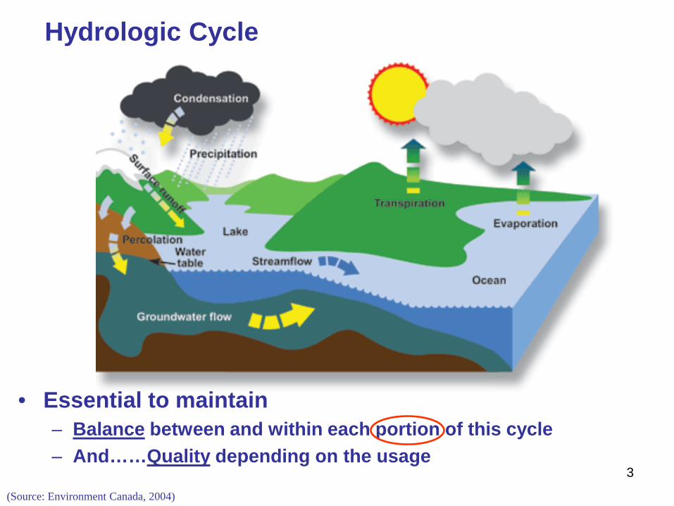
(Source: Environment Canada, 2004)

Hydrologic Cycle

• Essential to maintain – Balance between and within each portion of this cycle – And……Quality depending on the usage

3

Hydrologic Balance Atmospheric Water

Soil Water Surface Water

Groundwater

Change of Storage = Inflow - Outflow

Input SYSTEM

Output

OItS

−=∆∆

4

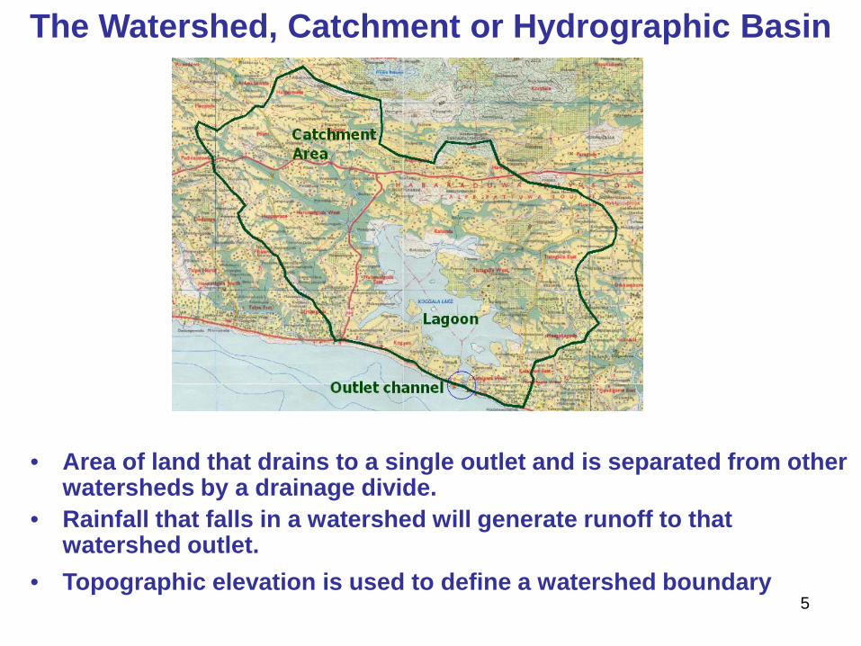
The Watershed, Catchment or Hydrographic Basin

• Area of land that drains to a single outlet and is separated from other watersheds by a drainage divide.

• Rainfall that falls in a watershed will generate runoff to that watershed outlet.

• Topographic elevation is used to define a watershed boundary 5

Watershed water balance

P

ET

O

Gout

Gin

S

OGETGPtS

outin −−−+=∆∆

6

Example: On November 1st in a certain year, water level of Kandalama tank is 174.1 m MSL. During November, average inflow (due to catchment runoff) and outflow (mainly for irrigation) of the tank are 6 m3/s and 5m3/s. Monthly average rainfall and evaporation in November are 400 mm and 120mm. Assuming negligible seepage loss and groundwater inflow into the reservoir, calculate the tank water level at the end of the month. Area capacity curve of Kandalama tank

Write the water balance equation for the tank, Inflow-outflow=change in the storage (runoff+rainfall) – (outflow+evaporation) = storage change

( ) ( ){ } ( ) ( ){ }

( ) ( ){ }

MSL m 174.8 is level water MCM 24.09At MCM 09.2419.994.10 storagemonth theof End

change storage 104.10change storage 1065.096.122.1615.55

change storage104.510120302436005104.510400302436006

6

6

6363

=+==×

=×+−+

=×××+×××−×××+××× −−

Storage (MCM)

7

Major Hydrologic Processes

• Precipitation (measured by radar or rain gauge)

• Evaporation and Transpiration (loss to atmosphere)

• Infiltration (loss to subsurface soils)

• Overland flow (sheet flow towards nearest stream)

• Stream flow (flow in streams and rivers)

• Groundwater flow and well mechanics

• Water quality and contaminant transport

8

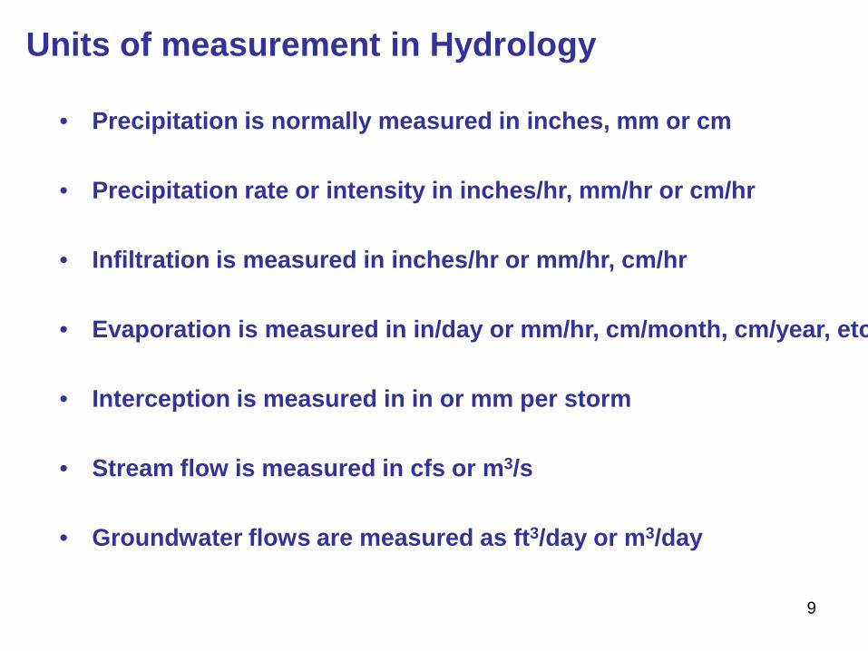
• Precipitation is normally measured in inches, mm or cm

• Precipitation rate or intensity in inches/hr, mm/hr or cm/hr

• Infiltration is measured in inches/hr or mm/hr, cm/hr

• Evaporation is measured in in/day or mm/hr, cm/month, cm/year, etc

• Interception is measured in in or mm per storm

• Stream flow is measured in cfs or m3/s

• Groundwater flows are measured as ft3/day or m3/day

Units of measurement in Hydrology

9

Types of Water Resources

• Atmosphere: atmospheric water vapor rain, drizzle snow, glaze (rain below 0C), sleet (frozen rain drops, transparent) , hail (large ice particles)

• Surface waters: rivers, lakes, oceans, ice caps, glaciers

• Groundwater: soil moisture, aquifers, vadose water (water existing

above the water table)

10

• 73%-agriculture purposes • 21%-industrial • 6%-domestic

World-Wide Water Consumption

(Source: World Commission on Water, 1999)

Sri Lanka –

140 litres (Rural)

185 litres (Urban) (NWS&DB design guidelines)

11

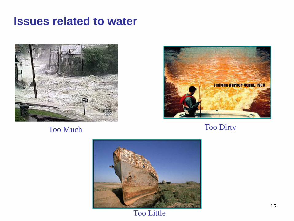
Issues related to water

Too Much Too Dirty

Too Little 12

Precipitation- Formation, Measurement and Analysis

13

Precipitation – various forms • Rain (most important)

• Snow (significant in cold countries)

• Hail (confined to short periods)

14

Precipitation mechanisms

• Condensation occurs when relative humidity reaches 100 %

• A condensation nucleus is needed • “Mechanism of cooling” is essential

15

Climatic Controls

• Continentality

• Direction of prevailing storm systems

• Topography

• Orientation of Topography

• Altitude

• Location with respect to the jet stream

16

Types of precipitation

Orographic precipitations - lifting over mountain ranges Convective precipitation - heating at or near surface, common in hot days Frontal precipitation – due to hot/ cold air masses Cyclonic precipitations – Frontal, low pressure systems 17

Frontal Precipitation

In this figure, the storm is moving toward the right and is being continually supplied with warm, moist, low-level air at its leading edge. In the updraft fed by this inflow, condensation produces rain above the freezing temperature and snow at lower temperatures. To the rear of the storm, dry middle-level air flows into the storm. As evaporation of rain cools this air, it becomes negatively buoyant and sinks. When the resulting downdraft reaches the ground, it spread out and forms the gust front. 18

Hurricane, Typhoon or Cyclone – Counterclockwise rotation (N hemisphere) and vice-versa in S

Tornado – Short-lived – Wind velocity up to 800 km/h!!!

19

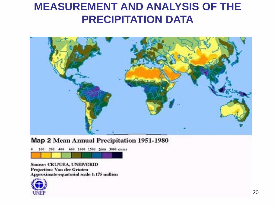
MEASUREMENT AND ANALYSIS OF THE PRECIPITATION DATA

20

Average seasonal rainfall in Sri Lanka

21

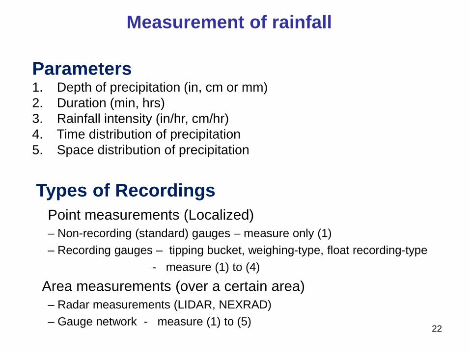
Measurement of rainfall

Parameters 1. Depth of precipitation (in, cm or mm) 2. Duration (min, hrs) 3. Rainfall intensity (in/hr, cm/hr) 4. Time distribution of precipitation 5. Space distribution of precipitation

Types of Recordings Point measurements (Localized) – Non-recording (standard) gauges – measure only (1) – Recording gauges – tipping bucket, weighing-type, float recording-type - measure (1) to (4)

Area measurements (over a certain area) – Radar measurements (LIDAR, NEXRAD)

– Gauge network - measure (1) to (5)

22

Tipping Bucket Rain Gauge

Recording gauge

Collector and Funnel

Bucket and Recorder

23

0.00

10.00

20.00

30.00

40.00

50.00

60.00

12/2

5/57

12:0

0 AM

12/2

5/57

6:00

AM

12/2

5/57

12:0

0 PM

12/2

5/57

6:00

PM

12/2

6/57

12:0

0 AM

12/2

6/57

6:00

AM

Rai

nfal

l (m

m)

A rainfall record (event: 25th Dec 1957 at Anuradapura)

24

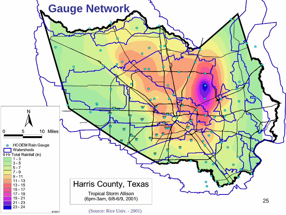
(Source: Rice Univ. - 2001)

Gauge Network

25

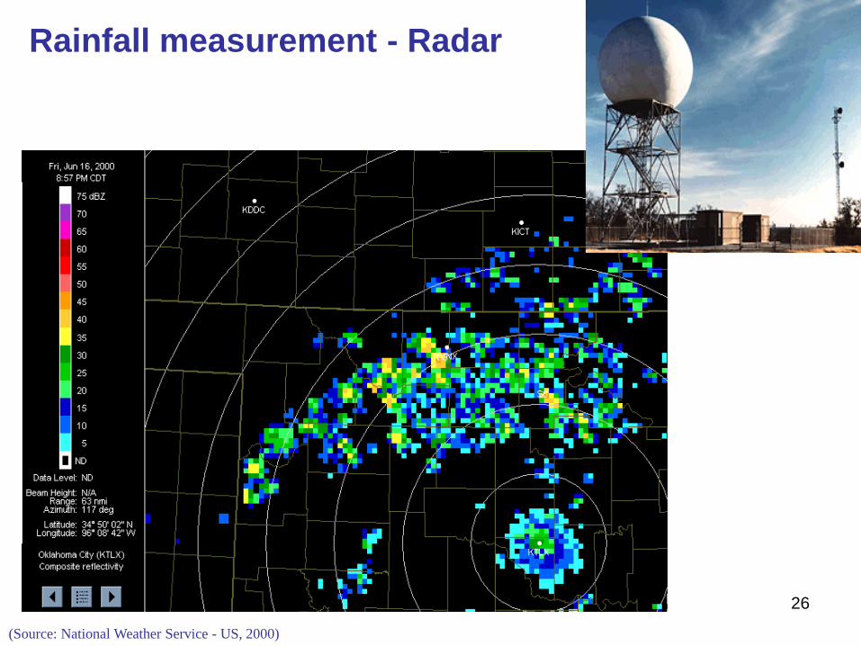
(Source: National Weather Service - US, 2000)

Rainfall measurement - Radar

26

1. Recent Innovation

2. Digital data is recorded every

5 min over each grid cell as

storm advances (eg: 4 km x 4

km cells)

3. The radar data can be

summed over a storm to

provide total rainfall depths

by sub-areas

4. Accurate to 150-250 km2

5. Provides spatial detail better

than gauges

Rainfall measurement - Radar

27

28

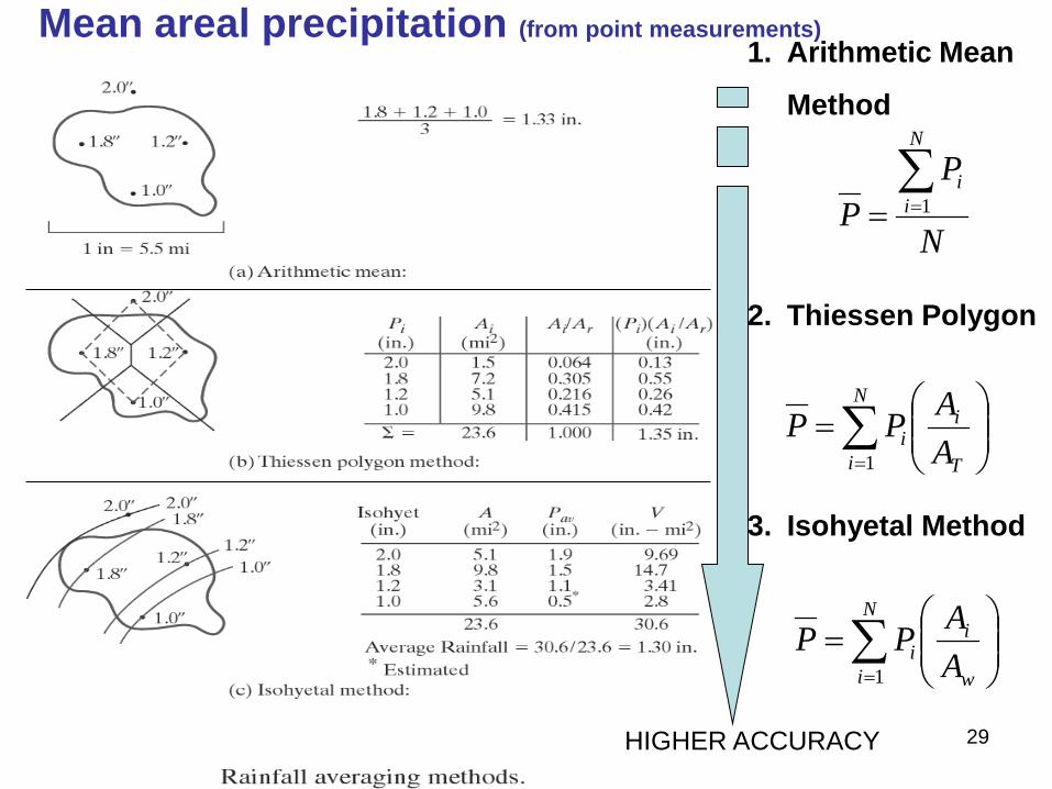
Mean areal precipitation (from point measurements) 1. Arithmetic Mean

Method

2. Thiessen Polygon

3. Isohyetal Method

N

PP

N

ii∑

== 1

∑=

=

N

i T

ii A

APP1

HIGHER ACCURACY

∑=

=

N

i w

ii A

APP1

29

Thiessen Polygons – Average

precipitations

1. Connect gauges with lines

2. Form triangles as shown

3. Create perpendicular bisectors

of the triangles

4. Each polygon is formed by lines

and catchment boundary

30

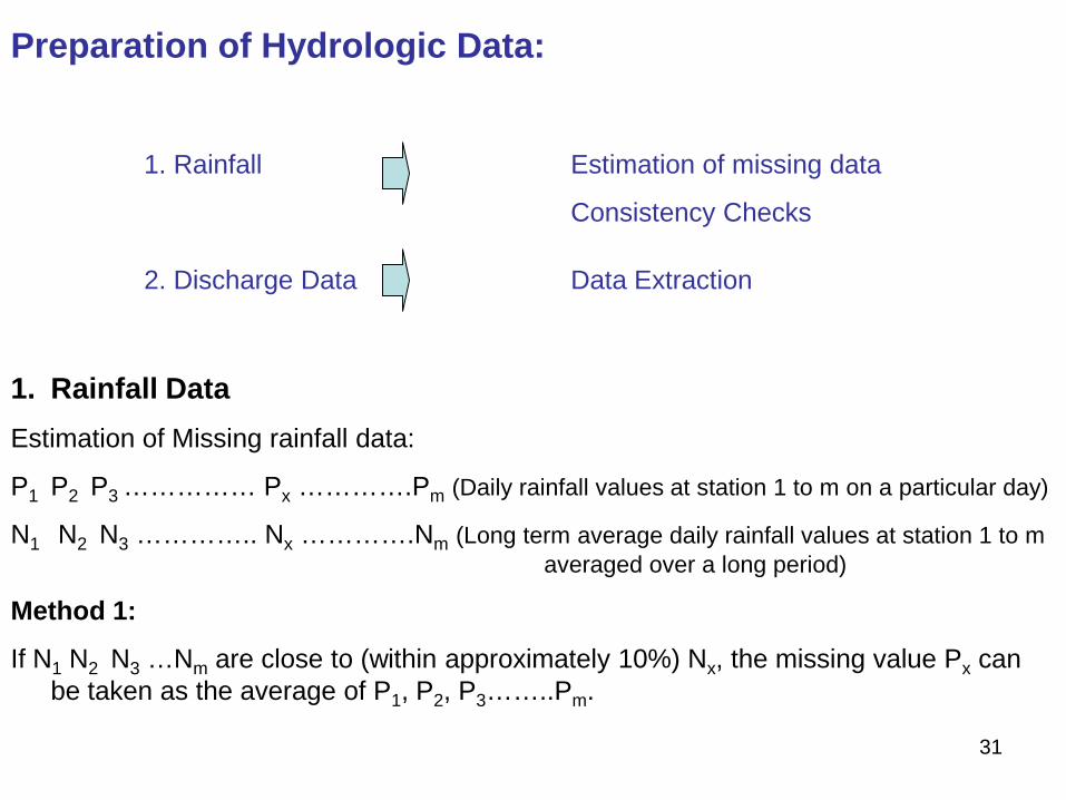
Preparation of Hydrologic Data:

1. Rainfall Estimation of missing data

Consistency Checks

2. Discharge Data Data Extraction

1. Rainfall Data Estimation of Missing rainfall data:

P1 P2 P3 …………… Px ………….Pm (Daily rainfall values at station 1 to m on a particular day)

N1 N2 N3 ………….. Nx ………….Nm (Long term average daily rainfall values at station 1 to m averaged over a long period)

Method 1:

If N1 N2 N3 …Nm are close to (within approximately 10%) Nx, the missing value Px can be taken as the average of P1, P2, P3……..Pm.

31

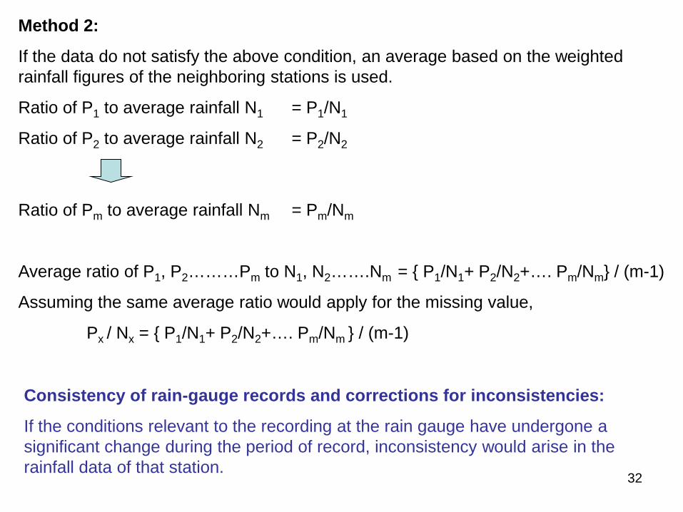
Method 2:

If the data do not satisfy the above condition, an average based on the weighted rainfall figures of the neighboring stations is used.

Ratio of P1 to average rainfall N1 = P1/N1

Ratio of P2 to average rainfall N2 = P2/N2

Ratio of Pm to average rainfall Nm = Pm/Nm

Average ratio of P1, P2………Pm to N1, N2…….Nm = { P1/N1+ P2/N2+…. Pm/Nm} / (m-1)

Assuming the same average ratio would apply for the missing value,

Px / Nx = { P1/N1+ P2/N2+…. Pm/Nm } / (m-1)

Consistency of rain-gauge records and corrections for inconsistencies:

If the conditions relevant to the recording at the rain gauge have undergone a significant change during the period of record, inconsistency would arise in the rainfall data of that station.

32

Some of the causes for inconsistency are;

1. Changing the location of the rain gauge

2. Neighborhood of rain gauge undergone a significant change

3. Change of ecosystem due to large scale forest fires, land slides etc.

4. Occurrence of an observation error from a certain date.

Inconsistency can be found by the double mass curve technique.

Assume,

P - Reading at the station under consideration

Pav - Average of corresponding readings at surrounding stations

The values of P and Pav are summed up as cumulative totals in the reverse chronological order (ie, first (old) reading last and last (new) reading first)

33

∑P

∑Pav

New records

Old records

Old records are brought to new regime by,

Pcorrected = Precorded x { corrected slope / original slope }

34

2. Stream Flow Data

h

hi

35

( ) 28.02.0 VVVi +=

∑=

∆=n

iiii WVQ

1

36

In certain cases (floods), it is difficult to measure velocity. For some sections one can measure the geometrical characteristics of cross-sectional area and channel slope and use Manning equation to obtain the streamflow, Q.

Estimation of streamflow - Slope-area method

Manning’s Equation used to estimate flow rates

Q = (1/n) A R 2/3 S 1/2

Where Q = flow rate (m3/s)

n = Manning roughness coefficient (empirical)

A = cross sectional area (m2)

R = hydraulic radius = A / P (m)

S = Slope (head loss per unit length of channel)

37

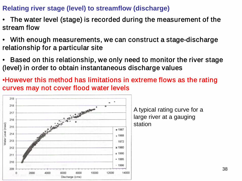
Relating river stage (level) to streamflow (discharge) • The water level (stage) is recorded during the measurement of the stream flow

• With enough measurements, we can construct a stage-discharge relationship for a particular site

• Based on this relationship, we only need to monitor the river stage (level) in order to obtain instantaneous discharge values

•However this method has limitations in extreme flows as the rating curves may not cover flood water levels

A typical rating curve for a large river at a gauging station

38

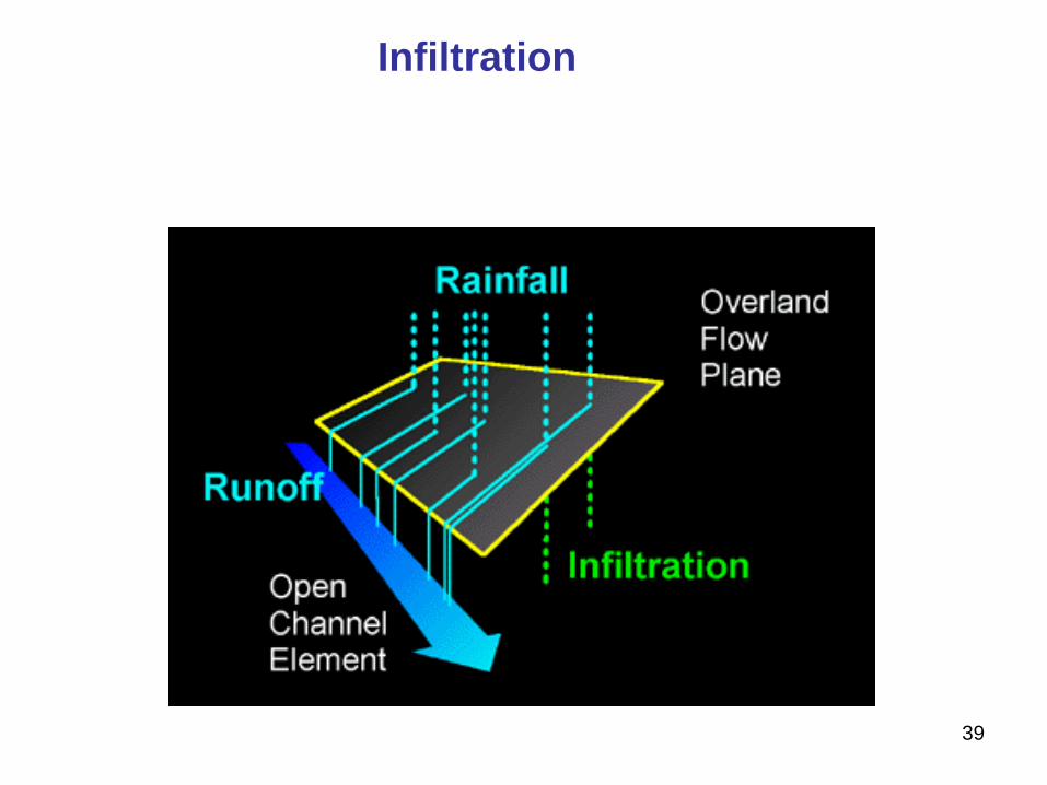
Infiltration

39

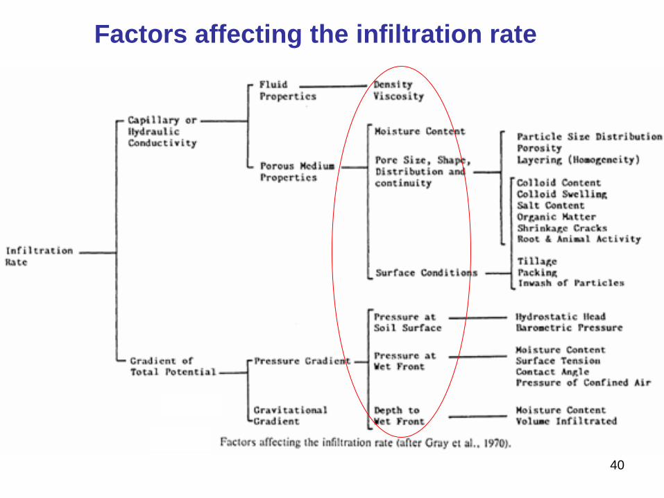
Factors affecting the infiltration rate

40

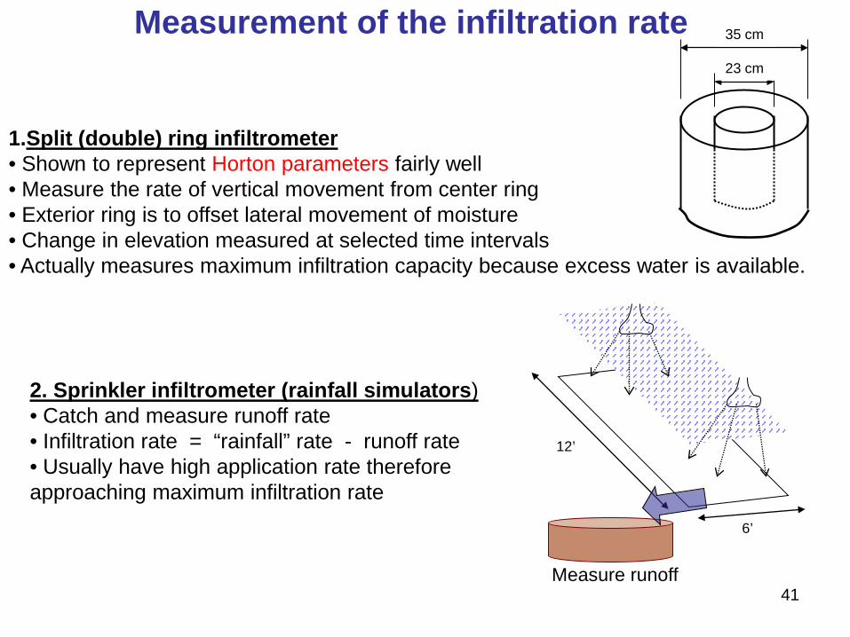
Measurement of the infiltration rate

12’

6’

1.Split (double) ring infiltrometer • Shown to represent Horton parameters fairly well • Measure the rate of vertical movement from center ring • Exterior ring is to offset lateral movement of moisture • Change in elevation measured at selected time intervals • Actually measures maximum infiltration capacity because excess water is available.

2. Sprinkler infiltrometer (rainfall simulators) • Catch and measure runoff rate • Infiltration rate = “rainfall” rate - runoff rate • Usually have high application rate therefore approaching maximum infiltration rate

35 cm

23 cm

Measure runoff 41

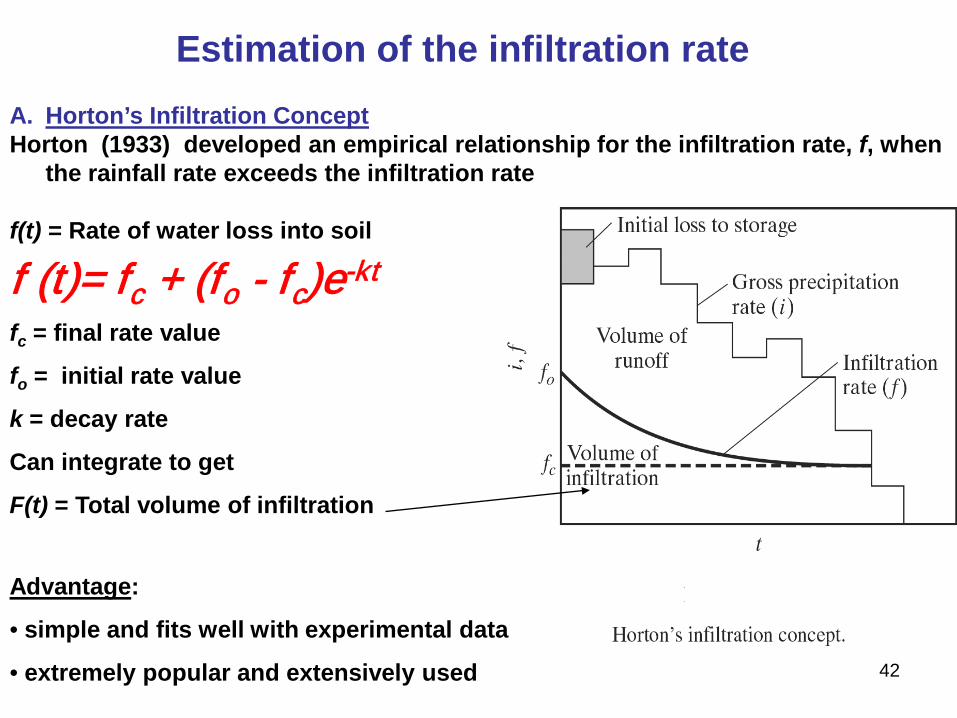
Estimation of the infiltration rate A. Horton’s Infiltration Concept Horton (1933) developed an empirical relationship for the infiltration rate, f, when

the rainfall rate exceeds the infiltration rate f(t) = Rate of water loss into soil

f (t)= fc + (fo - fc)e-kt fc = final rate value

fo = initial rate value

k = decay rate

Can integrate to get

F(t) = Total volume of infiltration

Advantage:

• simple and fits well with experimental data

• extremely popular and extensively used 42

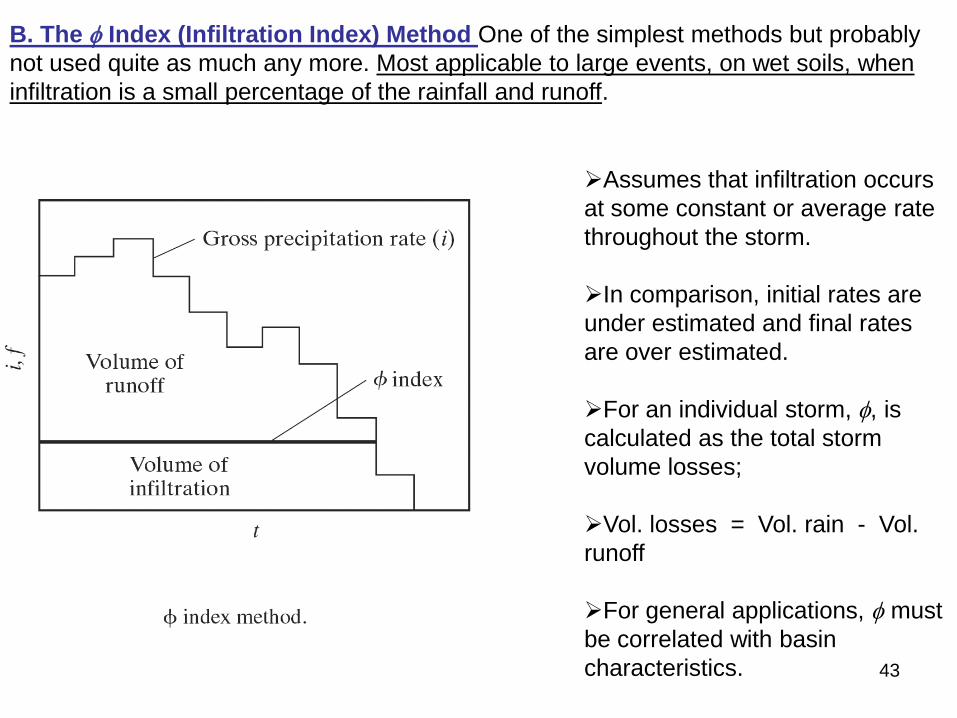
B. The φ Index (Infiltration Index) Method One of the simplest methods but probably not used quite as much any more. Most applicable to large events, on wet soils, when infiltration is a small percentage of the rainfall and runoff.

Assumes that infiltration occurs at some constant or average rate throughout the storm. In comparison, initial rates are under estimated and final rates are over estimated.

For an individual storm, φ, is calculated as the total storm volume losses;

Vol. losses = Vol. rain - Vol. runoff

For general applications, φ must be correlated with basin characteristics.

43

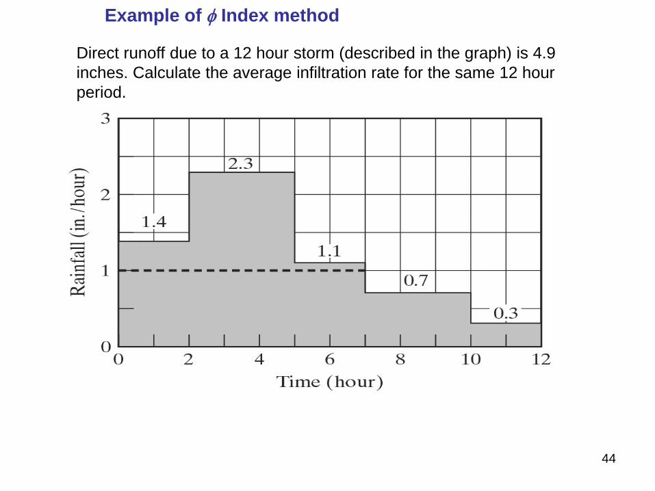
Example of φ Index method

Direct runoff due to a 12 hour storm (described in the graph) is 4.9 inches. Calculate the average infiltration rate for the same 12 hour period.

44

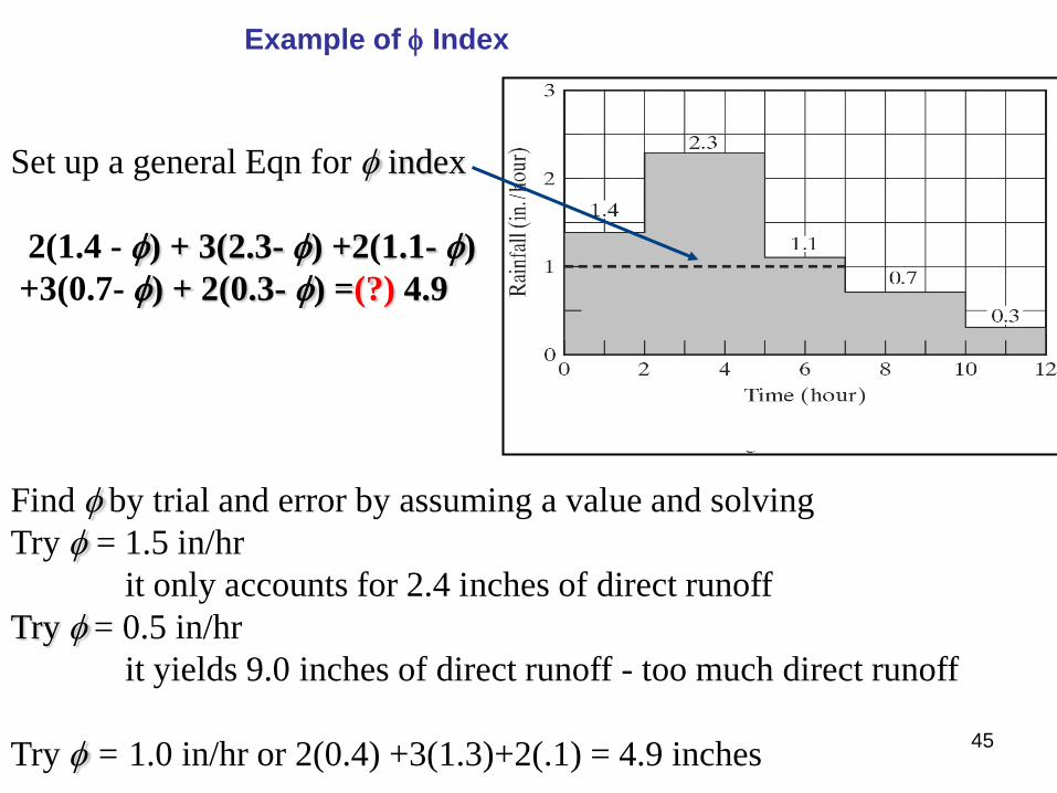
Example of φ Index

Set up a general Eqn for φ index 2(1.4 - φ) + 3(2.3- φ) +2(1.1- φ) +3(0.7- φ) + 2(0.3- φ) =(?) 4.9 Find φ by trial and error by assuming a value and solving Try φ = 1.5 in/hr it only accounts for 2.4 inches of direct runoff Try φ = 0.5 in/hr it yields 9.0 inches of direct runoff - too much direct runoff Try φ = 1.0 in/hr or 2(0.4) +3(1.3)+2(.1) = 4.9 inches 45

Hydrologic Design Hydrologic design is the process of assessing the impact of hydrological events on a project and choosing values for the key variables of the project so that it will function properly throughout its design lifetime.

Hydrologic designs are done for two types of projects;

1. Water Control Projects

Ex: Drainage and flood control, salinity and sediment control etc.

2. Water Use Projects

Ex: Water supply systems, irrigation, hydropower generation etc.

In both types of projects, main task is to determine a design flow to,

1. route the flow through the system

2. check whether the discharge values are satisfactory

Design for water control is concerned with extreme events of short duration, such as instantaneous peak discharge during a flood (to assess the capacity of structures etc.) or the minimum flow over a period of few days during a dry period (to ensure sediment control)

Design for water use is concerned with the complete flow hydrograph over a period of several years. 46

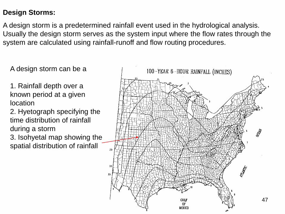
Design Storms:

A design storm is a predetermined rainfall event used in the hydrological analysis. Usually the design storm serves as the system input where the flow rates through the system are calculated using rainfall-runoff and flow routing procedures.

A design storm can be a 1. Rainfall depth over a known period at a given location 2. Hyetograph specifying the time distribution of rainfall during a storm 3. Isohyetal map showing the spatial distribution of rainfall

47

0.00

50.00

100.00

150.00

200.00

250.00

300.00

350.00

0 10 20 30 40 50 60 70 80 90 100 110 120

Rai

nfal

l Int

ensi

ty (m

m/h

r)

Duration (min)

RAINFALL INTENSITY DURATIOIN FREQUENCY CURVES STATION COLOMBO

2Yr 10Yr 50Yr 100Yr

Design hyetographs from IDF curves 1. Alternating block method

Design return period and the total duration of the rainfall should be selected first. Hyetograph ordinates are obtained from the IDF curve.

Select a time interval ∆t and find the ordinates of hyetograph at 1∆t, 2∆t, 3∆t,………n∆t. Where n ∆t is the total duration of the hyetograph.

1∆t 2∆t

I1

I2 Time Intensity Hyetograph ordinates

1∆t 2∆t 3∆t . . n∆t

I1 I2 I3 In

H1 = I1 ∆t H2 = I2 2∆t - I1 ∆t H3 = I3 3∆t – I22 ∆t

48

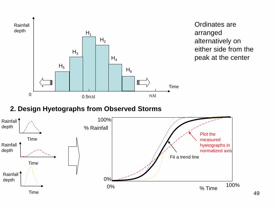
H1 H2

H3 H4

H5 H6

Rainfall depth

Time

0 n∆t 0.5n∆t

Ordinates are arranged alternatively on either side from the peak at the center

2. Design Hyetographs from Observed Storms Rainfall depth

Time Rainfall depth

Time

Rainfall depth

Time % Time

% Rainfall

100% 0%

100%

0%

Plot the measured hyetographs in normalized axis

Fit a trend line

49

Plot all available extreme event storms in normalized axis and fit a trend line. This trend line gives the shape of the design storm. However the magnitude of the design storm should be calculated separately. Cumulative rainfall depth of the design storm can be calculated using a statistical method (ex. Gumbel’s method) with daily rainfall values. Spread this cumulative value in the hyetograph using the shape established by the trend line.

Design Discharges

1. RATIONAL METHOD

Q = C I A where: Q = peak runoff rate, m3/s C = runoff coefficient, non-dimensional I = rainfall intensity, mm/hr A = area, km2

I can be read from the IDF curves. C is given in text books. This is the easiest method to calculate discharge for a known rainfall intensity. Assumptions: Rainfall occurs uniformly over the entire watershed. Rainfall occurs with a uniform intensity for a duration equal to the time of concentration for the watershed. The runoff coefficient, C, is dependent upon physical characteristics of the watershed, e.g. soil type.

50

51

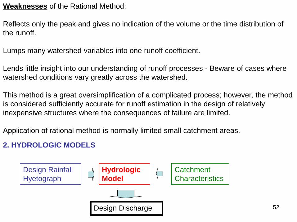
Weaknesses of the Rational Method: Reflects only the peak and gives no indication of the volume or the time distribution of the runoff. Lumps many watershed variables into one runoff coefficient. Lends little insight into our understanding of runoff processes - Beware of cases where watershed conditions vary greatly across the watershed. This method is a great oversimplification of a complicated process; however, the method is considered sufficiently accurate for runoff estimation in the design of relatively inexpensive structures where the consequences of failure are limited. Application of rational method is normally limited small catchment areas.

2. HYDROLOGIC MODELS

Hydrologic Model

Design Rainfall Hyetograph

Catchment Characteristics

Design Discharge 52