hydrological procedure no. 5 catchments in peninsular...

HYDROLOGICAL PROCEDURE NO. 5

RATIONAL METHOD OF FLOOD ESTIMATION FOR RURAL CATCHMENTS IN PENINSULAR MALAYSIA

DIVISION OF WATER RESOURCES MANAGEMENT AND HYDROLOGY DEPARTMENT OF IRRIGATION AND DRAINAGE

MINISTRY OF NATURAL RESOURCES AND ENVIRONMENT

2010

i

DISCLAIMER

Although every effort and care has been taken in selecting the methods and proposing

the recommendations that are appropriate to Malaysian conditions, the user is wholly

responsible to make use of this hydrological procedure. The use of this procedure

requires professional interpretation and judgment to suit the particular circumstances

under consideration.

The department or government shall have no liability or responsibility to the user or any

other person or entity with respect to any liability, loss or damage caused or alleged to

be caused, directly or indirectly, by the adaptation and use of the methods and

recommendations of this publication, including but not limited to, any interruption of

service, loss of business or anticipatory profits or consequential damages resulting

from the use of this publication.

ii

ACKNOWLEDGMENT

The Water Resources Management and Hydrology Division of the Department of

Irrigation and Drainage (DID), Ministry of Water Resources and Environment, Malaysia

would like to express sincere appreciation to USAINS Holding Sdn. Bhd, Associate

Professor Dr. Hj. Ismail Bin Abustan, Dr Choong Wee Kang and Associate Professor

Ahmad Shukri Bin Yahya in preparing this Hydrological Procedure. Valuable

contribution and feedbacks from DID personnel especially to the Director of Water

Resources Management and Hydrology Division, Ir. Hj. Hanapi Bin Mohamad Noor and

his staff namely Hj. Azmi Bin Md. Jafri, Mohd Khardzir Husain and Sazali Bin Osman

are greatly acknowledge.

iii

Table of Contents

Item Description

Page

Disclaimer i

Acknowledgment ii

Table of Contents iii

List of Tables v

List of Figures v

CHAPTER 1: INTRODUCTION 1

CHAPTER 2: THE RATIONAL METHOD AND FREQUENCY ANALYSIS 2

2.1 General 2

2.2 Features of the Rational Method 3

2.3 Hydrologic Frequency Analysis 3

CHAPTER 3: THE INVESTIGATION 5

3.1 General 5

3.2 Methodology of the Investigation 5

3.2.1 Design Sequence 5

3.2.2 Estimation of Time of Concentration 5

3.2.3 Estimation of the Average Intensity of the Design Storm 6

3.2.4 Estimation of Runoff Coefficient C 6

3.2.5 Regional Runoff Coefficient C based on Flood Frequency Regions

7

CHAPTER 4: ACCURACY OF THE PROCEDURE 10

4.1 Comparison with Observed Data 10

4.2 Comparison with HP5:1989 11

CHAPTER 5: LIMITATIONS OF THE PROCEDURE 12

CHAPTER 6: USE OF THE PROCEDURE 13

6.1 Components of the Procedure 13

6.2 Work Sequence 13

6.3 Worked Examples 14

References 18

iv

Appendix A A1 – A8

Appendix B1

Appendix B2

Appendix C

Appendix D

Appendix E

Appendix F

Appendix G

v

List of Tables

Table No.

Description

Page

Table 1 Dimensionless Runoff Coefficient CT for 18 Rural Catchments in this Study

7

Table 2 Regional Runoff Coefficient CT for Four Hydrological Regions 9

Table 3 Comparison of Results (Q10) of Various Methods 11

List of Figures

Table No.

Description

Page

Figure 1 Hydrological Regions in Peninsular Malaysia 8

Figure 2 Relation of Mean Frequency Factor CY/C10 for Different Regions 9

Figure 3 Scatter Diagram Comparing q10 Values Obtained from HP5:2010 and qpro and q10 Values Obtained from Observed Data qobs

11

1

1 INTRODUCTION

This hydrological procedure presents the results of a study on the applicability of a

Rational Method for flood estimation in small rural catchments in Peninsular Malaysia.

The Rational Method can be traced back to the mid-nineteenth century. The use of the

Rational Method in the urban environment has worked reasonably well in many

countries. For rural catchments, the use of the Rational Method has received much

criticism. Overseas researchers who have studied the method as a deterministic model

and tested it with observed data have found that the method offers low accuracy when

individual storms and resulting peak discharges are considered. However, studies by

French et al. (1974), who examined the validity of the method, have shown that,

statistically, the method serves the purpose of engineering practice, where peak

discharges of a given frequency are linked with the rainfall intensities of the same

frequency.

Given that the annual total expenditures on many small hydraulic structures, such as

bridges, culverts, diversion works, and so on, involve significant expense, the need for

a procedure to guide practitioners in arriving at a more reasonable design of such

structures is both urgent and important. For this purpose, the Department of Irrigation

and Drainage (DID) Hydrological Procedure No. 5 (HP5) is used as a basis for the

design of the above structures by most practitioners.

There are two earlier editions of HP5. The first edition was published in 1974

(HP5:1974) (Heiler, 1974), whereas the second was released in 1989 (HP5:1989)

(Azmi and Zahari, 1989). HP5:2010, the third edition, incorporates 18 rural catchments

in four hydrological regions. It uses Hydrological Procedure No. 1 (Fadhillah et al.,

1982) (HP1:1982) for the estimation of a design rainstorm.

2

2 THE RATIONAL METHOD AND FREQUENCY ANALYSIS

2.1 General

Hydraulic designs in engineering are composed of two main aspects: flood estimation

and channel sizing. The Rational Method is used for flood estimation. This method is

still widely used because of its simplicity; however, criticisms have been raised

regarding its use, and methods that are more advanced are available.

The Rational Method is typically used for peak runoff computation. According to Ojha et

al. (2008), the main considerations of the Rational Method are as follows:

The peak runoff rate is a function of the average rainfall rate during the time of

concentration; and

Rainfall intensity is constant during rainfall.

Based on the Rational Method, the main concept of HP5 lies in the statistical link

between the frequency distribution of the design rainfall and the design flood.

The Rational Method is known for its simplicity in the computation of design discharge.

Its inability to simulate individual storms and its unsuitability to observe peak discharge

have been criticized. However, in this case, the usefulness of the Rational Method

should be viewed from a different perspective: the statistical link between the frequency

of peak discharge and the design rainfall of the same frequency.

The statistical concept is the main idea of HP5, and is established in the relationship

between the peak discharge and the design rainfall of the same frequency. This differs

from other deterministic models because its judgment is based on the ability to

simulate flood events.

The Statistical Rational Method for the estimation of peak discharge is written as

AICQ TTT 278.0

Equation 1

where QT : Design peak discharge in m³/s, with return period of T years selected based on recommended design return period

CT : Dimensionless runoff coefficient as a function of catchment characteristics, design rainfall, and return period

IT : Average rainfall intensity of design rainfall in mm/h, with return period of T years and with rainfall duration being equal to the time of concentration

3

A : Catchment area in km²

Source: HP5:1989 (Azmi and Zahari, 1989)

2.2 Features of the Rational Method

The Rational Method is generally considered to be one of the best available flood

estimation procedures for small urban and rural catchment areas. However, there has

been much confusion concerning the principles underlying the method.

The Rational Method has been criticized because of its inability to reproduce particular

flood events when actual rainfall is used as the input. Such criticism implies an

assumption that the method is deterministic and does not represent the physical

operation on the rainfall–runoff process. This is not the intended use of the method.

The most realistic way to use the Rational Method is to consider it as a statistical link

between the frequency distribution of rainfall and runoff. As such, it provides a means

of estimating the design flood of a certain return period, with the rainfall duration equal

to the time of concentration.

Rewriting Equation 1,

AI

QC

T

TT 278.0

Equation 2

T

TT

I

qC

Equation 3

where CT : Dimensionless runoff coefficient, which represents the statistical link between the frequency of peak discharge (qT m³/s per km²) and the mean intensities of the design rainfall (IT mm/h) with return period of T years

qT : 0.278 QT/A is the peak discharge (qT m³/s per km²) and the mean intensities of the design rainfall (IT mm/h) with return period of T years. Peak runoff rate of return period T years is derived from the frequency analysis of the observed flood.

IT : Average rainfall intensity of the design rainfall in mm/h, with return period of T years and with rainfall duration equal to Tc, which is derived from frequency analysis of the recorded rainfall

A : Catchment area in km²


2.3 Hydrologic Frequency Analysis

Hydrologic frequency analysis involves the analysis of hydrologic data assumed to be

independent and identically distributed with the hydrologic system. These data are

considered to be stochastic, as well as space- and time-independent.

4

The aim of hydrologic frequency analysis is to relate the magnitude of extreme events

to their frequency of occurrence through probability distribution. In this case, the

magnitude of the extreme event is inversely related to its frequency of occurrence

(Chow et al., 1988).

Among various types of hydrologic data, the annual maximum discharge data are

utilized for frequency analysis in the current study. The outcome of frequency analysis

is the return period. In this case, the return period of an event of a given magnitude is

defined as the average recurrence interval between events equal to or exceeding a

specified magnitude (Chow et al., 1988). This information is then utilized in the design

of various hydraulic structures, such as bridges and culverts for road crossings,

detention and retention basins, and others.

5

3 THE INVESTIGATION

3.1 General

This section, rather than describing in detail the development of the procedure, outlines

the general methodology employed by the general user. The frequency analyses of the

annual maximum flood data from the catchment are not covered; interested readers

should thus refer to DID Hydrological Procedure Nos. 1 and 4 for details.

3.2 Methodology of the Investigation

3.2.1 Design Sequence

In using the Rational Method for flood estimation, the usual design sequence is as

follows:

a) Estimate the critical duration of the design storm (made equal to Tc);

b) Compute the various values of mean intensity (IT) for duration equal to Tc;

c) Estimate the values of CT from storm- and flood-frequency regions; and

d) Compute the peak discharge (QT) for various values of Tc using Equation 1.

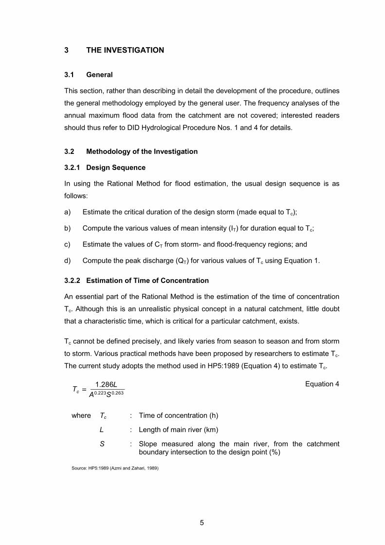
3.2.2 Estimation of Time of Concentration

An essential part of the Rational Method is the estimation of the time of concentration

Tc. Although this is an unrealistic physical concept in a natural catchment, little doubt

that a characteristic time, which is critical for a particular catchment, exists.

Tc cannot be defined precisely, and likely varies from season to season and from storm

to storm. Various practical methods have been proposed by researchers to estimate Tc.

The current study adopts the method used in HP5:1989 (Equation 4) to estimate Tc.

263.0223.0

286.1

SA

LTc

Equation 4

where Tc : Time of concentration (h)

L : Length of main river (km)

S : Slope measured along the main river, from the catchment boundary intersection to the design point (%)


6

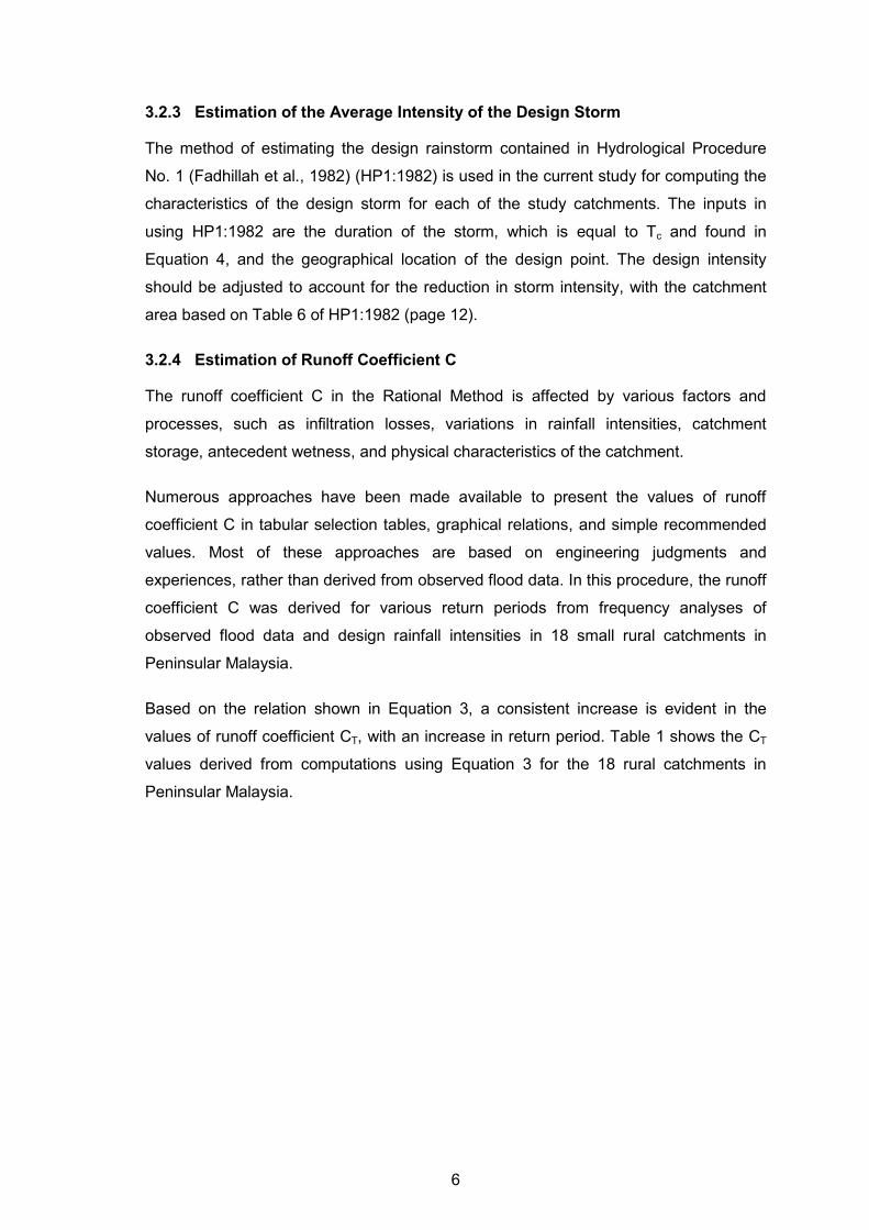
3.2.3 Estimation of the Average Intensity of the Design Storm

The method of estimating the design rainstorm contained in Hydrological Procedure

No. 1 (Fadhillah et al., 1982) (HP1:1982) is used in the current study for computing the

characteristics of the design storm for each of the study catchments. The inputs in

using HP1:1982 are the duration of the storm, which is equal to Tc and found in

Equation 4, and the geographical location of the design point. The design intensity

should be adjusted to account for the reduction in storm intensity, with the catchment

area based on Table 6 of HP1:1982 (page 12).

3.2.4 Estimation of Runoff Coefficient C

The runoff coefficient C in the Rational Method is affected by various factors and

processes, such as infiltration losses, variations in rainfall intensities, catchment

storage, antecedent wetness, and physical characteristics of the catchment.

Numerous approaches have been made available to present the values of runoff

coefficient C in tabular selection tables, graphical relations, and simple recommended

values. Most of these approaches are based on engineering judgments and

experiences, rather than derived from observed flood data. In this procedure, the runoff

coefficient C was derived for various return periods from frequency analyses of

observed flood data and design rainfall intensities in 18 small rural catchments in

Peninsular Malaysia.

Based on the relation shown in Equation 3, a consistent increase is evident in the

values of runoff coefficient CT, with an increase in return period. Table 1 shows the CT

values derived from computations using Equation 3 for the 18 rural catchments in

Peninsular Malaysia.

7

Table 1. Dimensionless Runoff Coefficient CT for 18 Rural Catchments in this Study

Item Catchment Dimensionless runoff coefficient, CT (qT/iT)

C2 C5 C10 C20 C50

1 Sg Arau 0.1777 0.2181 0.2292 0.2356 0.2430

2 Sg Buluh 0.5279 0.6309 0.6554 0.6684 0.7056

3 Sg Tasoh 0.0338 0.0408 0.0430 0.0443 0.0455

4 Sg Pelarit 0.1096 0.1156 0.1164 0.1164 0.1166

5 Sg Kulim 0.1653 0.3122 0.3595 0.4198 0.4624

6 Sg Chenderiang 0.0516 0.0698 0.0781 0.0871 0.0958

7 Sg Bernam 0.1307 0.2034 0.2311 0.2495 0.2763

8 Sg Lui 0.0661 0.1071 0.1263 0.1398 0.1527

9 Sg Kepis 0.4829 0.5981 0.6514 0.6546 0.6827

10 Sg Gemencheh 0.1046 0.1925 0.2467 0.2670 0.2967

11 Sg Pedas 0.0926 0.1106 0.1184 0.1313 0.1327

12 Sg Durian Tunggal 0.0597 0.0826 0.0957 0.1053 0.1132

13 Sg Kesang 0.0493 0.0601 0.0610 0.0612 0.0637

14 Sg Kemasin 0.5138 0.5792 0.6302 0.6646 0.6843

15 Sg Lanas 0.3126 0.4026 0.4432 0.4715 0.5146

16 Sg Chalok 0.3672 0.4708 0.5256 0.5644 0.5922

17 Sg Telemong 0.4770 0.4779 0.4842 0.4845 0.4857

18 Sg Penchala 0.3608 0.5771 0.6802 0.7763 0.8634

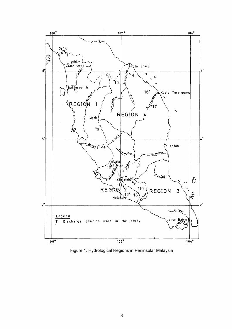
3.2.5 Regional Runoff Coefficient C based on Flood Frequency Regions

For the application of this procedure, Peninsular Malaysia was divided into four Flood

Frequency Regions (Figure 1) based on DID HP4:1987 (Ong, 1987) and HP5:1989

(Azmi and Zahari, 1989). The frequency distribution of flood peaks and flood-producing

rainstorms does not significantly affect the runoff coefficient C within the same region.

The mean values of the runoff coefficient for return periods of 2, 5, 10, 20, and 50

years were computed for each region. These values of C2, C5, C10, C20, and C50 are

presented in Table 2. The relation of mean frequency factor CY/C10 for different regions

is shown in Figure 2.

8

Figure 1. Hydrological Regions in Peninsular Malaysia

9

Table 2. Regional Runoff Coefficient CT for Four Hydrological Regions

Hydrological Regions

Dimensionless runoff coefficient, CT (qT/iT)

C2 C5 C10 C20 C50

Region 1 0.1554 0.2055 0.2224 0.2373 0.2534

Region 2 0.1233 0.1837 0.2118 0.2360 0.2602

Region 3 0.2948 0.4113 0.4395 0.4719 0.5036

Region 4 0.3955 0.4684 0.4928 0.5193 0.5421

Figure 2. Relation of Mean Frequency Factor CY/C10 for Different Regions

0.5

0.6

0.7

0.8

0.9

1.0

1.1

1.2

1.3

1 10 100

Return Period Y (Years)

Mean F

requency F

acto

r C

Y/C

10

Region 1 Region 2 Region 3 Region 4

10

4 ACCURACY OF THE PROCEDURE

Two methods were employed to evaluate the accuracy of the new procedure:

i. The first method compared 10-year design peak discharges estimated using the

new procedure with 10-year peak discharges of observed data derived using

single-station frequency analysis.

ii. The second method compared design peak discharges derived using the new

procedure with design peak discharges derived using HP5:1989.

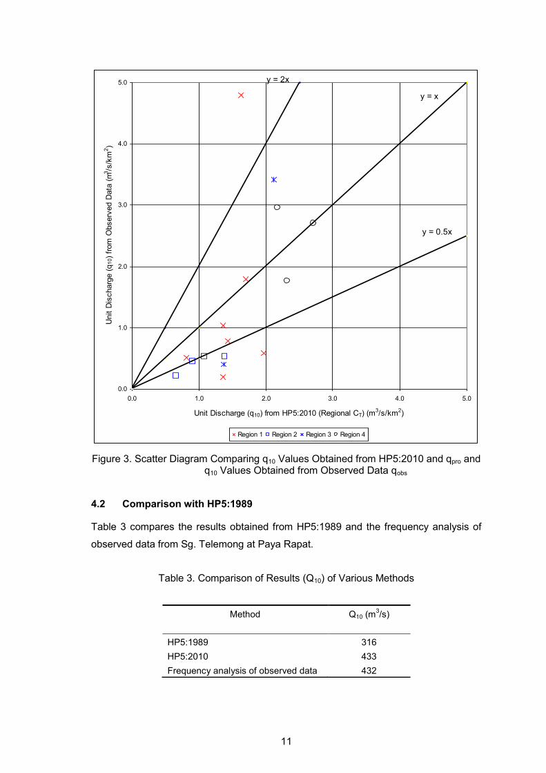
4.1 Comparison with Observed Data

The result of the comparison between 10-year design peak discharges estimated using

this procedure (based on Regional C10) with 10-year peak discharges of observed data

is presented as a scatter diagram. Figure 3 presents the scatter diagram for Regions 1,

2, 3, and 4.

11

Figure 3. Scatter Diagram Comparing q10 Values Obtained from HP5:2010 and qpro and q10 Values Obtained from Observed Data qobs

4.2 Comparison with HP5:1989

Table 3 compares the results obtained from HP5:1989 and the frequency analysis of

observed data from Sg. Telemong at Paya Rapat.

Table 3. Comparison of Results (Q10) of Various Methods

Method

Q10 (m3/s)

HP5:1989 316

HP5:2010 433

Frequency analysis of observed data 432

y = x

y = 2x

y = 0.5x

0.0

1.0

2.0

3.0

4.0

5.0

0.0 1.0 2.0 3.0 4.0 5.0

Unit Discharge (q10) from HP5:2010 (Regional CT) (m3/s/km2)

Unit D

ischarg

e (

q10)

from

Observ

ed D

ata

(m

3/s

/km

2)

Region 1 Region 2 Region 3 Region 4

12

5 LIMITATIONS OF THE PROCEDURE

From the theoretical basis of the Rational Method, two important factors are neglected:

(1) the effects of channel storage and (2) the temporal and spatial variations of rainfall

intensities. As a result of such limitations and because the procedure was derived

utilizing data from rural catchments with areas ranging from 3.9 to 186 km2, the use of

the procedure in estimating runoff for larger areas is not recommended. A multiplying

factor that considers catchment development (Appendix A) should serve as a general

guide to arrive at a reasonable estimate. However, there has been no study to

substantiate this recommendation. The procedure may not be reliable in estimating

runoff in areas with steep slopes. As a general guide, the slope value limit, as

developed by this procedure, is approximately 0.1%–5%. Similar to any other flood

estimation procedures, the design flood obtained from this procedure should be

checked with other available procedures, and the decision to adopt the estimated

design values should be complemented by sound engineering judgment.

13

6 USE OF THE PROCEDURE

6.1 Components of the Procedure

The following items are required to use this flood estimation procedure:

i. Figure 1. The general deposition of four regions proposed for application;

ii. Table 2. The regional runoff coefficient for four hydrological regions; and

iii. DID Hydrological Procedure No. 1 (Fadhillah et al., 1982) (HP1:1982),

“Estimation of the Design Rainfall in Peninsular Malaysia.”

6.2 Work Sequence

The detailed design sequence for using this procedure is as follows:

Step 1 Select a return period for the design (T1).

Step 2 Based on catchment characteristics, estimate the value of TC using Equation 4.

Step 3 Compute the depth of the design storm of duration TC for return periods of 2, 10, and 20 years. Estimates for return periods of 2 and 20 years are required to estimate the confidence limit of the design storm.

Step 4 Compute the confidence limit of X(T1, TC), which is estimated based on X(2, TC) and X(20, TC) values. Refer to HP1:1982 for a complete explanation.

Step 5 Compute the depth of the design storm of duration TC for return period T1.

Step 6 Estimate the value of C from Table 2.

Step 7 Compute the design discharge QT using Equation 1 and compute the confidence limits of the design discharge.

Step 8 Adjust QT based on a future land use scenario using factor F, which is listed in Appendix A.

14

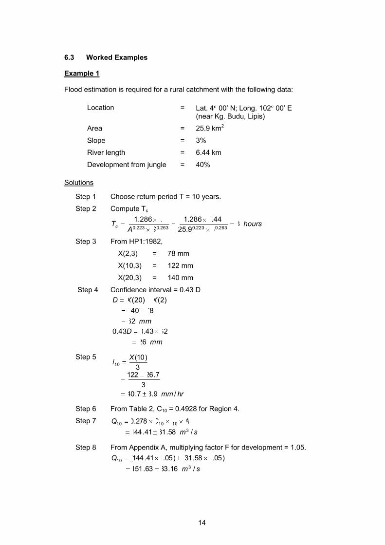
6.3 Worked Examples

Example 1

Flood estimation is required for a rural catchment with the following data:

Location = Lat. 4 00’ N; Long. 102 00’ E (near Kg. Budu, Lipis)

Area = 25.9 km2

Slope = 3%

River length = 6.44 km

Development from jungle = 40%

Solutions

Step 1 Choose return period T = 10 years.

Step 2 Compute Tc

hoursSA

LTc 3

39.25

44.6286.1286.1263.0223.0263.0223.0

Step 3 From HP1:1982,

X(2,3) = 78 mm

X(10,3) = 122 mm

X(20,3) = 140 mm

Step 4 Confidence interval = 0.43 D

mm

D

mm

XXD

26

6243.043.0

62

78140

)2()20(

Step 5

hrmm

Xi

/9.87.40

3

7.261223

)10(10

Step 6 From Table 2, C10 = 0.4928 for Region 4.

Step 7

sm

AiCQ

/58.3141.144

278.0

3

101010

Step 8 From Appendix A, multiplying factor F for development = 1.05.

sm

Q

/16.3363.151

)05.158.31()05.141.144(

3

10

15

Example 2

A flood estimate is required for a rural catchment. The following data relate to the

catchment:

Location = Lat. 4 00’ N; Long. 102 00’ E (near Kg. Budu, Lipis)

Area = 25.9 km2

Slope = 1%



Solutions


Step 2 Compute Tc

hoursSA

LTc 4

19.25

44.6286.1286.1263.0223.0263.0223.0


X(2,4) = 80 mm

X(10,4) = 98 mm

X(20,4) = 105 mm


mm

D

mm

XXD

7.10

2543.043.0

25

80105

)2()20(

Step 5

hrmm

Xi

/7.25.24

4

7.10984

)10(10

Step 6 From Table 2, C10 = 0.4928 for Region 4.

Step 7

sm

AiCQ

/58.993.86

278.0

3

101010

Step 8 From Appendix A, multiplying factor F for development = 1.05.

sm

Q

/06.1028.91

)05.158.9()05.193.86(

3

10

16

Example 3

Obtain a flood estimate for a culvert on a main trunk road. The following data relate to

the culvert and the catchment:

Location = Lat. 5 00’ N; Long. 103 00’ E

(near Kg. Pelandan, Hulu Terengganu)

Catchment area = 5.18 km2

Catchment slope = 5%



Solutions


Step 2 Compute Tc

hoursSA

LTc 406.1

518.5

44.6286.1286.1263.0223.0263.0223.0


X(2, 1.406) = 75 mm

X(10, 1.406) = 118 mm

X(20, 1.406) = 135 mm


mm

D

mm

XXD

8.25

6043.043.0

60

75135

)2()20(

Step 5 hrmm

Xi /4.180.83

4.1

8.25118

4.1

)10(10

hrmmX

i /4.180.964.1

8.25135

4.1

)20(20

Step 6 From Table 2, for Region 4,

C10 = 0.4928

C20 = 0.5193

Step 7

sm

AiCQ

/06.139.5818.5)4.1883(4928.0278.0

278.0

3

101010

sm

AiCQ

/76.138.7118.5)4.1896(5193.0278.0

278.0

3

202020

17

References:

Azmi, Md. J. and Zahari, O. (1989). Hydrological Procedure No. 5: Rational Method of

Flood Estimation for Rural Catchments in Peninsular Malaysia. Jabatan Pengairan dan

Saliran, Malaysia.

Chow, V.T., Maidment, D.R. and Mays, L.W. (1988). Applied Hydrology, McGraw-Hill,

New York, NY.

Mohd. Fadhlillah, M., Salena, S., Leong, T.M. and Teh, S.K. (1982). Hydrological

Procedure No.1: Estimation of the Design Rainstorm in Peninsular Malaysia (Revised

and Updated). Jabatan Pengairan dan Saliran, Malaysia.

Ong, C.Y. (1987). Hydrological Procedure No. 4: Magnitude and Frequency of Floods

in Peninsular Malaysia. Jabatan Pengairan dan Saliran, Malaysia.

Ong, C.Y. and Liam, W.L. (1986). Water Resources Publication No.17: Variation of

Rainfall with Area in Peninsular Malaysia. Jabatan Pengairan dan Saliran, Malaysia.

USACE (1993). Engineering Manual No.: EM 1110-2-1415, Engineering and Design,

Hydrologic Frequency Analysis. U.S. Army Corps of Engineer, Washington.

Water Resources Council. (1982). Guidelines for Determining Flood Flow Frequency,

Bulletin 17B, Hydrology Committee, Washington, D.C.

18

Appendix A. Multiplying Factors that Account for Catchment Development

Development to Agriculture from Jungle X (%)

Multiplying Factor (F)

0 < X ≤ 25 1.00

25 < X ≤ 50 1.05

50 < X ≤ 75 1.15

75 < X ≤ 100 1.20

Note: Multiply QT estimates from undeveloped area by Factor F.

Source: DID HP5 (1974)

Appendix G

G1

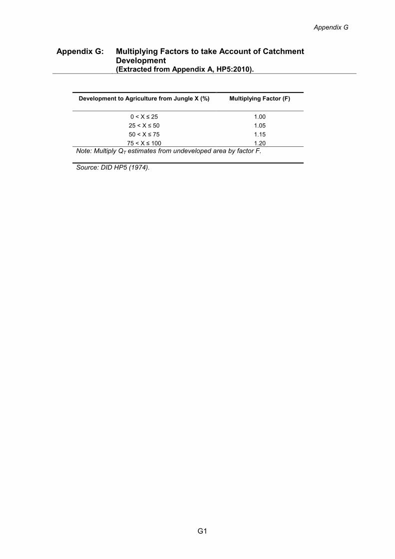
Appendix G: Multiplying Factors to take Account of Catchment Development (Extracted from Appendix A, HP5:2010).

Development to Agriculture from Jungle X (%)

Multiplying Factor (F)

0 < X ≤ 25 1.00

25 < X ≤ 50 1.05

50 < X ≤ 75 1.15

75 < X ≤ 100 1.20

Note: Multiply QT estimates from undeveloped area by factor F.

Source: DID HP5 (1974).

hydrological procedure no. 5 catchments in peninsular...

Documents