hydrologic response unit routing in swat to simulate effects of
TRANSCRIPT

Water 2011, 3, 819-842; doi:10.3390/w3030819
waterISSN 2073-4441
www.mdpi.com/journal/water
Article
Hydrologic Response Unit Routing in SWAT to Simulate Effects
of Vegetated Filter Strip for South-Korean Conditions
Based on VFSMOD
Youn Shik Park 1, Jeong Hee Park
2, Won Seok Jang
3, Ji Chul Ryu
3, Hyunwoo Kang
3,
Joongdae Choi 3 and Kyoung Jae Lim
3,*
1 Department of Agricultural and Biological Engineering, Purdue University, West Lafayette,
IN 47907, USA; E-Mail: [email protected] 2 Depatment of Environmental Science, Kangwon National University, 2 Hyoja-dong, Chuncheon,
Gangwon Province, South Korea; E-Mail: [email protected] 3 Depatment of Regional Infrastructure Engineering, Kangwon National University, 2 Hyoja-dong,
Chuncheon, Gangwon Province, South Korea; E-Mails: [email protected] (W.S.J.);
[email protected] (J.C.R.); [email protected] (H.K.); [email protected] (J.C.)
* Author to whom correspondence should be addressed; E-Mail: [email protected];
Tel.: +82-33-250-6468; Fax: +82-33-251-1518.
Received: 21 March 2011; in revised form: 11 August 2011 / Accepted: 15 August 2011 /
Published: 26 August 2011
Abstract: The Soil and Water Assessment Tool (SWAT) model has been used worldwide
for many hydrologic and Non-Point Source (NPS) Pollution analyses on a watershed scale.
However, it has many limitations in simulating the Vegetative Filter Strip (VFS) because it
considers only ‘filter strip width’ when the model estimates sediment trapping efficiency
and does not consider the routing of sediment with overland flow which is expected to
maximize the sediment trapping efficiency from upper agricultural subwatersheds to lower
spatially-explicit filter strips. Therefore, the SWAT overland flow option between
landuse-subwatersheds with sediment routing capability was enhanced by modifying the
SWAT watershed configuration and SWAT engine based on the numerical model
VFSMOD applied to South-Korean conditions. The enhanced SWAT can simulate the VFS
sediment trapping efficiency for South-Korean conditions in a manner similar to the desktop
VFSMOD-w system. Due to this enhancement, SWAT is applicable to simulate the effects
of overland flow from upper subwatersheds to reflect increased runoff volume at the lower
OPEN ACCESS
Water 2011, 3
820
subwatershed, which occurs in the field if no diversion channel is installed. In this study, the
enhanced SWAT model was applied to small watersheds located at Jaun-ri in South-Korea
to simulate a diversion channel and spatially-explicit VFS. Sediment can be reduced by
31%, 65%, and 68%, with a diversion channel, the VFS, and the VFS with diversion
channel, respectively. The enhanced SWAT should be used in estimating site-specific
effects on sediment reduction with diversion channels and VFS, instead of the currently
available SWAT, which does not simulate sediment routing in overland flow and does not
consider other sensitive factors affecting sediment reduction with VFS.
Keywords: Vegetative Filter Strip; HRU Routing; SWAT; VFSMOD
1. Introduction
In recent years, sediment transport in runoff has been considered one of the serious environmental
problems in South-Korea as well as other countries [1,2], there are many methods to prevent soil
erosion and sediment inflow into water bodies, through structural and non-structural best management
practices (BMPs) to prevent or manage sediment transport. Vegetative Filter Strip (VFS) is one of
most effective BMPs to reduce sediment load and pollutants from agricultural fields [3-8]. VFS is
usually installed at the edge of agricultural areas or the areas along streams, and it is designed to
remove not only sediment load but also other pollutants, such as nutrients from runoff by filtration,
infiltration, adsorption, absorption, deposition, decomposition, and plant uptake [4]. The dimension of
VFS needs to be determined from experimental data under various field and rainfall conditions to
obtain the desired pollutant removal results. However, these data are rarely available for site-specific
design of VFS. Thus, a physically-based model, capable of simulating the sediment behavior both in
VFS and sediment source areas such as agricultural areas, has been used to design the site-specific
dimensions of the VFS for expected VFS efficiency. To maximize the effects of VFS on sediment
reduction, the amount of runoff volume coming from the upper areas is often controlled with a
diversion channel. Significant amounts of runoff can flow into the agricultural area if an agricultural
area is located as a lower subwatershed to extensive forest areas. Moreover, if a diversion channel is
not installed, the chances are that soil erosion in the agricultural area will be increased by runoff from
the forest. Thus, both VFS and the diversion channel are often utilized together to increase sediment
deposition and reduce runoff flowing into agricultural areas from upper forest areas. The effects of
VFS and diversion channel need to be evaluated before installation in fields to maximize the effects of
sediment reduction and to determine the best places and dimensions of VFS and diversion channels.
The semi-distributed, continuous daily time step, and watershed-scale, Soil and Water Assessment
Tool (SWAT) model [9,10] has been extensively applied to watersheds [11-15], and has been used
as an effective tool for assessing watershed management plans on hydrologic and water quality
impacts [16-18]. The SWAT model divides the watershed into subwatersheds, and they are further
divided into Hydrologic Response Units (HRUs), which are unique combinations of land use/cover
and soil types within each subwatershed. In the current SWAT model/interface, the SWAT model does
not simulate overland flow and overland flow-driven sediment from upper subwatersheds to lower
Water 2011, 3
821
subwatersheds; only channelized flow and sediment transport through stream networks are simulated if
the SWAT ArcView GIS interface is used in delineating subwatersheds and stream networks [19].
Thus, the effects of spatially explicit VFS and diversion channels cannot be simulated with the current
SWAT model/interface. The effect of VFS for sediment reduction, moreover, is simulated as a
function of only VFS width in the current SWAT, although many other factors affect the trapping
efficiency of the VFS [4,20-23]. Thus, the current SWAT needs to be enhanced to properly model VFS
and diversion channels for sediment reduction analysis.
The objectives of this study were to modify SWAT to enable flow and sediment routing (either
overland or channelized flow) from upper to lower subwatershed to simulate spatially explicit VFS and
diversion channels. We also aim to enhance the SWAT VFS module based on the numerical model
VFSMOD to consider upland runoff volume and filter width together for more accurate evaluation of
VFS efficiency within SWAT for South-Korean conditions.
2. Materials and Methods
2.1. Limitations of the SWAT for VFS and Diversion Channel Simulation
2.1.1. Limitation of SWAT for Flow and Sediment Routing in Overland Flow
The SWAT model simulates hydrology and water quality from each field (HRU) in the
subwatershed, and then simulates flow, sediment, chemicals, and nutrient changes through the stream
network with simulated values for all HRUs in each subwatershed. The model reflects various field
conditions at a watershed scale. Although the model has been widely used for various researches and
applications in many countries over the years, it has limitations in simulating some processes. One of
the limitations is the capability of overland flow simulation between an upper subwatershed (i.e.,
single-landuse subwatershed, such as agricultural field) and lower subwatershed (i.e., single-landuse
subwatershed, such as Vegetated Filter Strip). To simulate effects on flow and sediment reduction of
various BMPs using SWAT, the subwatersheds (single-landuse subwatershed) are often delineated
based on field boundaries and flow paths at micro-scales. To simulate the effects of VFS and diversion
channels with SWAT, subwatersheds need to be configured as shown in Figure 1 (single landuse
subwatershed for forest and single landuse-subwatershed for agricultural field, i.e., FRST and AGRL),
and the flow type needs to be modified so it is described as either overland flow or channelized flow,
or sometimes both flow types, depending on the field flow condition. As shown in Figure 1(a), SWAT
users need to specify the overland flow option manually with edits in the “fig.fig” SWAT watershed
configuration file, which is not an easy task for most SWAT users. In the current SWAT model,
sediment routing for overland flow conditions is not enabled as shown in Figure 1(b).
Water 2011, 3
822
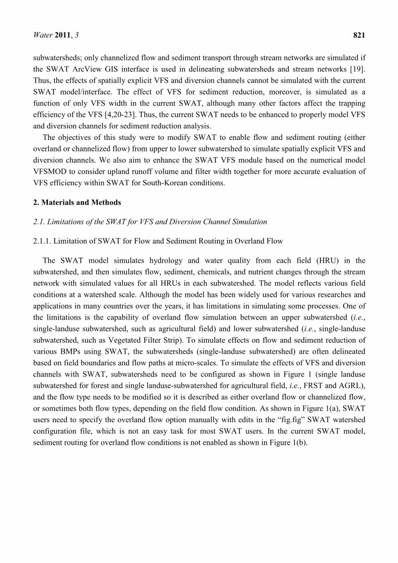
Figure 1. Limitation of the current Soil and Water Assessment Tool (SWAT) model for
overland flow and sediment routing.
(a) Channelized flow which is default option in current SWAT GIS interface.
(b) No sediment routing under overland flow condition, also, no overland flow option
enabled in the SWAT ArcView GIS interface.
Through modification of the model and revision of the “fig.fig” that is configuration file of the
model, overland flow and sediment routing by overland flow was able to be simulated between
subwatersheds to evaluate the effects on sediment reduction by the VFS and diversion channel, which are
commonly utilized BMPs in South-Korea and other countries to reduce sediment leaving source areas.
Water 2011, 3
823
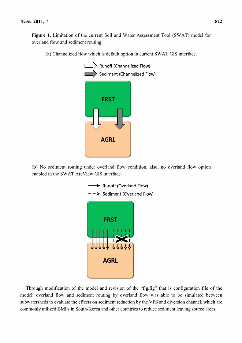
The current SWAT engine/interface assumes only channelized flows are dominant flow types and
flow routing is determined when delineating the subwatersheds and stream networks. Thus, to simulate
the effects of the VFS and the diversion channels properly, flow type and flow routing need to be
modified to reflect the water flow patterns occurring in the real field. Figure 2 partially shows the
‘fig.fig’ file which was modified for our study. Column 1 is the command to route (i.e., 2) or add
(i.e., 5) to other storage, the numbers in column 2 represent the hydrograph storage locations which
identify the result location after routing simulations. The numbers in column 3 are the reach that the
inflow and inputs are routed through, which are identical to the subwatershed numbers if they are
written on route command rows. The numbers in column 4 are hydrograph storage locations which
contain the data to be routed through the reach. The numbers in column 6 are area fractions of overland
flow volume, and if they have no values or ‘0’, it assumes a 100% channelized flow [19]. When the
user modifies the file, the number which is already taken as a hydrograph storage location number
cannot be overlapped, and the hydrograph storage number cannot be duplicated.
Figure 2. Revision of SWAT configuration file for diversion channel and Vegetative Filter
Strip (VFS) simulation.
To simulate overland flow type between subwatersheds (single-landuse subwatersheds), flow type
between upper a single landuse subwatershed and lower single landuse subwatershed needs to be

Water 2011, 3
824
defined manually before SWAT routing, which is confusing and time-consuming even for experienced
SWAT users. Although the revision of the file is not convenient, it is required to mimic the flow in the
real field that is hardly considered to be channelized flow in the real field. The limitation of the model
is that it does not consider the transportation of sediment from the upper subwatershed to the lower
subwatershed under ‘overland flow’ option, only sediment transport through the stream networks is
simulated. Therefore, spatially distributed VFS in the model does not receive sediment occurred in
upper subwatersheds.
Only the filter strip width parameter named ‘FILTHW’ is available to estimate the reduction of
pollutants, based on a regression equation derived from other studies [19]. Figure 3 shows how the
model estimates the effects of VFS on sediment reduction. The model estimates VFS by assuming that
there is no flow and sediment coming from other places, and that only sediment generated from the
agricultural fields (single landuse subwatershed) is reduced with no spatially explicit VFS defined by
the parameter.
Figure 3. Limitation of the current SWAT for VFS simulation–No spatial location of the
VFS in sediment reduction simulation with the VFS. Only filter width is considered for
sediment reduction estimation.
To simulate the effects of VFS and diversion channels in the model with more accuracy, overland
flow type and sediment routing from upper to lower subwatershed, and spatially explicit VFS with
overland flow type specified need to be made, with modifications in the SWAT model engine and
interfaces. To define the spatially explicit VFS installed along agricultural fields, the area of the
agricultural field (AGRL) needs to be adjusted to the area of the VFS (Figure 4). In the current SWAT,
the spatial location of VFS is not considered, only VFS width specified in the SWAT input parameter
is used to estimate sediment reduction with the VFS. To correctly simulate the effects of VFS and
diversion channels together with SWAT, flow and sediment from forest areas (FRST) to agricultural
areas (AGRL) in overland flow (or with partially overland and partially concentrated flow types), also
from agricultural area (AGRL) to the VFS that is located at the edge of agricultural fields (Figure 4)
have to be simulated with modifications to the model. This is because the model and its interface are
unable to consider the spatial location of the VFS.

Water 2011, 3
825
Figure 4. Proposed Runoff and Sediment Simulation reflecting spatially-explicit VFS.
2.1.2. Limitation of SWAT to Estimate Sediment Trapping Efficiency
As described earlier, both transported sediment by overland flow from upper to lower subwatershed
and spatially explicit VFS receiving overland flow need to be enabled in the simulation of VFS and
diversion channels with the model. However, the sediment trapping efficiency of the filter strip in the
model is only a function of filter strip width. Equation 1 shows the sediment trapping efficiency that is
used in the model [19].
trapef= 0.367 · (widthfilter strip)0.2967 (1)
Where trapef is sediment trapping efficiency and widthfilter strip is the width of the vegetative filter
strip (m).
However, numerous studies have shown that the sediment trapping efficiency of VFS is affected
by many factors, such as VFS slope, runoff volume from upland areas, soil type, and vegetation
characteristics [4,23,24]. Therefore, these factors need to be considered to evaluate pollutant reduction
efficiency of the VFS [24] in the VFS simulation. White and Arnold [25] suggested empirical models
to estimate sediment reduction efficiency based on runoff loading (mm), saturated hydraulic
conductivity (mm h−1), and sediment loading (kg/m
2).
When Equation (1) is used for sediment trapping efficiency simulation, the sediment trapping
efficiency becomes ‘1’ (i.e., 100% sediment trap with the VFS) with a filter width of 30 m or greater,
as shown in Figure 5, irrespective of the magnitude of the storm events and runoff generated from it.
Thus, the sediment trapping efficiency module of the SWAT needs to be enhanced or modified to
estimate sediment trapping efficiency reflecting other sensitive factors, such as runoff volume.

Water 2011, 3
826
Figure 5. Limitation of sediment trapping efficiency module in current SWAT.
2.2. Enhancement and Application of SWAT for VFS and Diversion Channel Simulation
2.2.1. Enhancement of SWAT for Flow and Sediment Routing in Overland Flow
The model has limitations in simulating diversion channels and spatially explicit VFS. The model
does not calculate sediment from upper subwatersheds to lower subwatersheds for overland flow, but
considers it only by channelized flow. Thus, in this study, the model was modified to route the
sediment from upper subwatersheds to lower subwatersheds with overland flow. This updated process
is used in the enhanced SWAT to simulate sediment routing from upper upland subwatersheds to lower
subwatersheds. The subroutine for the overland flow, called ‘RTOVER’, routes runoff from upper to
lower subwatersheds in overland flow. However, no sediment routing is enabled in this subroutine
under the ‘overland flow’ option. To consider sediment deposition in a field or subwatershed, the
area-based sediment delivery ratio by Vanoi [26] was used in the modified subroutine.
As shown in Figure 6, the ‘ROUTE’ subroutine calls the ‘RTOVER’ subroutine when the overland
flow option is given in SWAT. Runoff and pollutant loads, except sediment, are transferred to the
receiving watershed in the ‘RTOVER’ subroutine in SWAT and these values are used in the ‘ROUTE’
subroutine. In this study, the ‘RTOVER’ subroutine was modified to transfer sediment from upper
subwatersheds to lower subwatersheds after considering the area-based sediment delivery ratio to
explain potential sediment deposition.

Water 2011, 3
827
Figure 6. Enhancement of SWAT Sediment Routing under Overland Flow Type
Enhancement of Filter Strip Module in the Current SWAT.
(a) Current SWAT model (b) Enhanced SWAT model
Although the sediment trapping efficiency of filter strips is affected by not only the filter width but
also other factors, the filter strip subroutine (named ‘READHRU’ for SWAT2000 and ‘READMGT’
for SWAT2005) considers only filter strip width when it calculates sediment trapping efficiency using
Equation 1, and the reduced sediment is calculated in the subroutine ‘FILTER’ of both SWAT2000
and SWAT2005. One of the most effective models to simulate VFS is the Vegetative Filter Strip
Modeling System. The model is a field-scale, mechanistic, and storm-based numerical model. The
model simulates hydrograph in the source area and calculates outflow, infiltration, and sediment
trapping efficiency through VFS [4,21,22,27,28]. Park et al. [23] used the desktop-based VFSMOD-w
model [29,30] to identify the most sensitive factors affecting the sediment trapping efficiency and
derived a regression equation (Equation 2) to explain VFSMOD-w model behaviors with filter strip
width and incoming overland flow volume, which were the most sensitive factors regarding 10,000
VFSMOD-w runs with various field and rainfall conditions [23]. The EI and R2 values for the
comparison of the VFSMOD-w simulated results with the values from the regression equations were
0.99 and 0.98, respectively [23], indicating that the regression equation with filter width and incoming
runoff volume from source areas could explain the VFSMOD-w behaviors.

Water 2011, 3
828
Sediment Trapping Efficiency =
(−0.00007345046 × L3 + 0.001558 × L
2 − 0.006376×L −0.001189) × ( ln(V) )
3 +
(0.0009688469 × L3 − 0.020779 × L
2 + 0.095153 × L + 0.019348) × ( ln(V) )
2 +
(−0.004274 × L3 + 0.092846 × L
2 −0.487355 × L − 0.10563) × ( ln(V) ) +
(0.006381 × L3 − 0.140713 × L
2 + 0.869293 × L + 0.19386)
(2)
Where L is filter strip width, V is overland flow volume from field.
The subroutine ‘READMGT’ in the current SWAT reads the filter width parameter ‘FILTERW’,
and then calculates the sediment trapping efficiency with only filter width using Equation 1. With this
trapping efficiency, the subroutine ‘FILTER’ in the current SWAT calculates runoff and pollutant
reduction with the VFS (Figure 7(a)). In this study, the ‘TRAPEFF_VFSMOD’ module was written
and added to SWAT to calculate sediment reduction with Equation (2) to consider the sediment
trapping efficiency with the filter width and runoff volume (Figure 7(b)). Thus, the enhanced
VFSMOD-W based module of SWAT can simulate the VFS sediment trapping efficiency for
South-Korean conditions in a manner similar to the desktop VFSMOD-W system, since the EI and R2
values were 0.99 and 0.98, respectively.
Figure 7. Enhancement of the SWAT Filter Strip Module.
(a) Current SWAT Filter Strip Module (b) Enhanced SWAT Filter Strip Module
2.2.2. Application of Enhanced SWAT for VFS and Diversion Channel Effects Simulation
In this study, a small study watershed, located in Jaun-ri, Gangwon province, South-Korea, was
selected to simulate the effects of a diversion channel and VFS on sediment reduction with the
enhanced SWAT, which were not possible to simulate with the currently available SWAT model
(SWAT 2000/2005). The study watershed, located at coordinate 37°42’32’’N 128°21’34’’E, has two
dominant land uses; forest (23.83 ha, 96.17%) and agriculture (1.06 ha, 3.83%). The study watershed
soils are composed of clay 7.8%, silt 28.2%, and sand 63%. Maximum and minimum annual

Water 2011, 3
829
precipitation was 1,876 mm and 867 mm from 2000–2006 with an annual average precipitation of
1,396 mm. Approximately 60% of annual precipitation is concentrated during the summer in the
watershed, causing significant soil erosion and sediment yield. Average temperature ranged from
−24.6~36.5 °C, with a mean temperature of 11.21 °C. Extensive highland agricultural farming is
performed at the downstream areas of the study watershed (Figure 8). Thus, the South-Korea
government designated this area as a nonpoint source pollutant hotspot area. It is expected that various
soil erosion Best Management Practices (BMPs) will be introduced in the study watershed to reduce
soil erosion and sediment yields.
Figure 8. Location of Study Watershed–Jaun-ri Watershed, Gangwon, South-Korea.
Four scenarios were planned to compare the effects on sediment reduction of a diversion channel
and VFS as shown in Table 1. Scenario 1 represented the current situation with no BMPs. Scenario 2
included diversion channel and was compared with scenario 1 to investigate the effects of a diversion
channel on sediment reduction. Scenario 3 included VFS, the results were compared with scenario 1 to
identify the effects of the VFS. Scenario 4 included both diversion channel and the VFS, it was
compared with scenario 1 to determine the effects of both diversion channel and the VFS. Scenarios 3
and 4 were compared to investigate the effects on sediment reduction of the VFS with and without a
diversion channel.

Water 2011, 3
830
Table 1. Summary of Scenarios.
Diversion Channel VFS
Scenario 1 Non-Existence Non-Existence
Scenario 2 Existence Non-Existence
Scenario 3 Non-Existence Existence
Scenario 4 Existence Existence
In this study, 24 subwatersheds for simulations of scenarios 1 and 2 (diversion channel simulation)
(Figure 9) and 26 subwatersheds for simulations of scenarios 3 and 4 (VFS simulation) (Figure 10)
were delineated for application of the enhanced SWAT model with an agricultural area boundary
burned with the DEM for isolation of the agricultural area as a separate subwatershed (i.e.,
single-landuse subwatershed). To simulate (1) overland flow/sediment from forest watersheds to the
agricultural area for diversion channel effect; (2) overland flow/sediment from the agricultural area to
VFS for VFS effect, the 24 and 26 subwatersheds were regrouped as shown in Figure 11 and Figure 12
to explain effects of diversion channel and the VFS on sediment reduction.
Figure 9. Subwatersheds Delineated for Simulation of Diversion Channel.

Water 2011, 3
831
Figure 10. Subwatersheds Delineated for Simulation of VFS.
Figure 11. Twenty-four Subwatersheds and Four Subwatersheds Groups for Diversion
Channel Simulation.

Water 2011, 3
832
Figure 12. Twenty-Six Subwatersheds and Five Subwatershed Groups for Diversion
Channel and VFS Simulation.
For the simulations of scenarios 1 and 2 with 24 subwatersheds, the 1st subwatershed group
(denoted as SG1 hereafter) includes subwatersheds 1, 4, 5, 11, 10, and 22 which are the upper
subwatersheds of the agricultural area (subwatershed marked with no. 2). The 2nd subwatershed group
(denoted as SG2 hereafter) is the agricultural area (subwatershed marked with no. 2). The 3rd
subwatershed group (denoted as SG3 hereafter) includes forest dominant subwatersheds. For the 3rd
subwatershed group, subwatersheds numbered 6–9 and 12–21, no overland flow type was specified
because the flow and sediment from the 3rd subwatershed group do not affect sediment with the
diversion channel and VFS at the agricultural area, marked as the 2nd subwatershed group (i.e.,
subwatershed no. 2) in Figure 11. The 4th subwatershed group (denoted as SG4 hereafter) includes
subwatersheds 3, 23, and 24. For simulation of scenarios 3 and 4 with 26 subwatersheds, the 1st
subwatershed group (denoted as SG1 hereafter) includes subwatersheds 1, 6, 7, 12, 13, and 24 which
are the upper subwatersheds of the agricultural area (subwatershed marked with no. 2). The 2nd
subwatershed group (denoted as SG2 hereafter) is the agricultural area (subwatershed marked
with no. 2). The 3rd subwatershed group (denoted as SG3 hereafter) includes forest dominant
subwatersheds. For the 3rd subwatershed group, subwatersheds numbered 8–11 and 14–23, no
overland flow type was specified because the flow and sediment from the 3rd subwatershed group do
not affect sediment with the diversion channel and VFS at the agricultural area, marked as the 2nd
subwatershed group (i.e., subwatershed no. 2) in Figure 12. The 4th subwatershed group (denoted as
SG4 hereafter) includes subwatersheds 5, 25, and 26. The 5th subwatershed group (denoted as SG
5
hereafter) contains only subwatershed no. 4 which is spatially-explicit filter strips.

Water 2011, 3
833
2.2.3. Effect of Diversion Channel on Sediment Reduction
As stated before, the current SWAT model cannot simulate the effects of a diversion channel
because SWAT is not a fully distributed model, but is rather a semi-distributed model. To
verify sediment reduction effects of a diversion channel, two scenarios (scenarios 1 and 2)
were created as shown in Figure 13. Flow and sediment from SG1 flow into SG
2 as overland flow, and
flow and sediment from SG2 and SG
3 flow into SG
4 in “Scenario 1–no diversion channel”. For
“Scenario 2–diversion channel”, the flow and sediment from the SG1 do not flow into SG
2, instead
those flow into SG4 through a diversion channel. Scenarios 1 and 2 were run with modification in the
file named ‘fig.fig’ (watershed routing structure file in the SWAT2005) manually (Figure 13).
Figure 13. Watershed Configuration for Diversion Channel Simulation with
Enhanced SWAT.
2.2.4. Effect of Diversion Channel and Diversion Channel with VFS on Sediment Reduction
To verify sediment reduction effects of a diversion channel and VFS, two scenarios (Scenario 3 and
Scenario 4) were created as shown in Figure 14. The subwatersheds were rearranged with modification
in the file “fig.fig” to be compatible with “Scenario 3 and Scenario 4” overland flow and channelized
flow (Figure 14). It is assumed that flow and sediment from SG1 flow into SG
2 as overland flow, and
flow and sediment from SG2 flow into VFS subwatershed group SG
5 as overland flow, and flow and
sediment from SG3 and SG
5 flow into SG
4 as channelized flow for “Scenario 3–with VFS”. For
“Scenario 4–with VFS and diversion channel”, flow and sediment from SG1 flow directly into SG
4,
and flow and sediment from SG2 flow into VFS subwatershed group SG
5 (Figure 14). First, sediment
reduction with the VFS was analyzed by comparing the sediment values from Scenarios 1 and 3 with
the enhanced SWAT. Second, sediment reduction with VFS and a diversion channel was analyzed
with Scenarios 1 and 4. Third, sediment reduction of a diversion channel when the VFS is installed at
the edge of the agricultural areas was analyzed with Scenarios 3 and 4.

Water 2011, 3
834
Figure 14. Watershed Configuration for VFS and Diversion Channel with VFS Simulation
with Enhanced SWAT.
3. Results
3.1. Effects of Diversion Channel on Sediment Reduction (Scenario 1 vs. Scenario 2)
Average monthly flow rates at the watershed outlet from Scenarios 1 and 2 were 0.01387 m3/s and
0.01390 m3/s, respectively (Table 2). The maximum flow value of scenario 1 was 0.13860 m
3/s in July
2006, and the minimum value was 0.00003 m3/s in February 2005. The maximum flow value of
scenario 2 was 0.13860 m3/s in July 2006, and the minimum value was 0.00003 m
3/s in February 2005.
There was very little difference in estimated flow rates with a diversion channel, as expected.
However, the average monthly sediment values of scenarios 1 and 2 were 2.69 metric tons and 1.85
metric tons, respectively. The maximum sediment value of scenario 1 was 39.85 metric tons in July
2006, and the minimum value was 0.00013 metric tons in February 2005. The maximum monthly
average sediment value of scenario 2 was 33.84 metric tons in July 2006, and the minimum value was
0.00011 metric tons in February 2005. For the entire simulation period (2000–2006), it is expected that
a diversion channel can reduce sediment by 31% (Figure 15).
Table 2. Flow Rate and Sediment Load.
Flow Rate(m
3/s) Sediment Load(ton/month)
minimum average maximum minimum average maximum
Scenario 1 0.00003 0.01387 0.13860 0.00013 2.687 39.850
Scenario 2 0.00003 0.01390 0.13860 0.00011 1.854 33.840
Scenario 3 0.00023 0.01184 0.11750 0.00007 0.933 6.263
Scenario 4 0.00005 0.01194 0.11860 0.00011 0.860 14.650

Water 2011, 3
835
Figure 15. Comparison of Simulated Monthly Sediment for Scenarios 1 and 2.
3.2. Effects of VFS on Sediment Reduction (Scenario 1 vs. Scenario 3)
Average monthly flow rates of scenarios 1 and 3 were 0.014 m3/s and 0.012 m
3/s, respectively
(Table 2). The maximum flow value of scenario 3 was 0.118 m3/s in July 2006, and the minimum
value was 0.00023 m3/s in February 2005. There was little difference in the estimated flow rates with
VFS, as expected. The average monthly sediment values of scenarios 1 and 3 were 2.69 metric tons
and 0.93 metric tons, respectively. The maximum monthly average sediment value of scenario 3 was
6.26 metric tons in July 2006, and the minimum value was 0.00007 metric tons in February 2005. For
the entire simulation period (2000–2006), it is expected that sediment can be reduced with VFS at the
study watershed by 65% (Figure 16).
Figure 16. Comparison of Simulated Monthly Sediment for Scenarios 1 and 3.

Water 2011, 3
836
3.3. Effects of VFS with Diversion Channel on Sediment Reduction (Scenario 1 vs. Scenario 4)
Average monthly flow rates of scenarios 1 and 4 were 0.0139 m3/s and 0.0119 m
3/s, respectively
(Table 2). The maximum flow value of scenario 4 was 0.119 m3/s in July 2006, and the minimum
value was 0.00005 m3/s in February 2005. There was little difference in estimated flow rates with
diversion channel and VFS together, as expected. The average monthly sediment values of scenarios 1
and 4 were 2.69 metric tons and 0.86 metric tons, respectively. The maximum monthly average
sediment value of scenario 4 was 14.65 metric tons on July 2006, and the minimum value was 0.00011
metric tons on February 2005. For the entire simulation period (2000–2006), it is expected that 68% of
sediment can be reduced with a combined diversion channel and VFS in the study watershed
(Figure 17).
Figure 17. Comparison of Simulated Monthly Streamflow for Scenarios 1 and 4.
3.4. Effect of Diversion Channel when VFS is Installed at the Edge of the Agricultural Area
(Scenario 3 vs. Scenario 4)
As stated above, average monthly flow rate of scenarios 3 and 4 were 0.01184 m3/s and
0.01194 m3/s, respectively. There was little difference in estimated flow rates with the diversion
channel when VFS is installed at the edge of the agricultural areas, as expected. The average monthly
sediment values of scenario 3 and scenario 4 were 0.93 metric tons and 0.86 metric tons, respectively.
The maximum values of scenarios 3 and scenario 4 were 6.26 and 14.65 metric tons on July 2006,
respectively, and minimum values were 0.00007 and 0.00011 metric tons of scenarios 3 and scenario 4
on February 2005, respectively. For the entire simulation period (2000–2006), it is expected that
sediment can be reduced at the study watershed outlet by an additional 3% when a VFS is combined
with a diversion channel compared only to the diversion channel (Figure 18).
Water 2011, 3
837
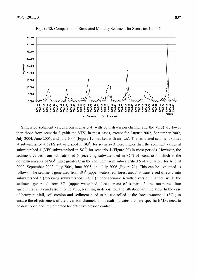
Figure 18. Comparison of Simulated Monthly Sediment for Scenarios 1 and 4.
Simulated sediment values from scenario 4 (with both diversion channel and the VFS) are lower
than those from scenario 3 (with the VFS) in most cases, except for August 2002, September 2002,
July 2004, June 2005, and July 2006 (Figure 19, marked with arrows). The simulated sediment values
at subwatershed 4 (VFS subwatershed in SG5) for scenario 3 were higher than the sediment values at
subwatershed 4 (VFS subwatershed in SG5) for scenario 4 (Figure 20) in most periods. However, the
sediment values from subwatershed 5 (receiving subwatershed in SG4) of scenario 4, which is the
downstream area of SG5, were greater than the sediment from subwatershed 5 of scenario 3 for August
2002, September 2002, July 2004, June 2005, and July 2006 (Figure 21). This can be explained as
follows: The sediment generated from SG1 (upper watershed, forest areas) is transferred directly into
subwatershed 5 (receiving subwatershed in SG4) under scenario 4 with diversion channel, while the
sediment generated from SG1 (upper watershed, forest areas) of scenario 3 are transported into
agricultural areas and also into the VFS, resulting in deposition and filtration with the VFS. In the case
of heavy rainfall, soil erosion and sediment need to be controlled at the forest watershed (SG1) to
ensure the effectiveness of the diversion channel. This result indicates that site-specific BMPs need to
be developed and implemented for effective erosion control.

Water 2011, 3
838
Figure 19. Comparison of Simulated Monthly Sediment for Scenarios 3 and 4.
Figure 20. Simulated Monthly Sediment at Subwatershed 4–receiving subwatershed in SG4.

Water 2011, 3
839
Figure 21. Simulated Monthly Sediment at Subwatershed 5–receiving subwatershed in SG4.
4. Conclusions and Discussion
The current SWAT model cannot be used to simulate the effects of diversion channels and VFS
because it cannot simulate the sediment routing with overland flow type between single landuse
subwatersheds, and the filter strip module of the current SWAT is only based on the filter strip width.
Thus, the sediment routing in overland flow type and filter strip module considering filter strip width with
the incoming runoff volume from source areas were enabled in the SWAT runs. Without considering
these aspects, the SWAT model cannot be used to simulate the effect of various non-structural soil erosion
BMPs on sediment reduction. In this study, a new VFS module reflecting the VFSMOD-w behaviors was
integrated with the SWAT engine codes and SWAT watershed and the flow configuration file, called
“fig.fig”, was modified manually to define overland flow type between subwatersheds.
The effect of a diversion channel and VFS for sediment reduction was analyzed using the enhanced
SWAT. The results showed that there was little difference in simulated flow at the watershed outlet, as
expected. However, it was found that a diversion channel and VFS were effective ways to reduce
sediment. Sediment reduction of 31% would be expected with a diversion channel, 65% with VFS, and
68% with the combined diversion channel and VFS for the study watershed.
This study showed that the enhanced SWAT should be used in estimating the site-specific effects on
sediment reduction with a diversion channel and the VFS, and the enhanced model needs to be
validated with measured data in the field to insure the predictive ability of the SWAT for the
site-specific assessment of soil erosion. The study was implemented with that VFS was distributed
spatially in the model, that sediment loading was estimated under overland flow condition, and that
sediment trapping efficiency by VFS was calculated by overland flow and filter strip width. However,
the empirical model to calculate sediment trapping efficiency needs to be evaluated through various

Water 2011, 3
840
applications to confirm that it is still effective in the SWAT model and that it is available to other
countries. The configuration file was revised to simulate the diversion channel, this work would hardly
be possible with other watersheds that have a huge number of subwatersheds in the model.
Acknowledgements
This research was supported by a grant (code: EW-07-II-06, Development of effective management
techniques for rural NPS pollution) from Eco-Star Project.
References
1. Brown, L.R. Conserving Soils. In State of the World; Brown, L.R., Ed.; Norton: New York, NY,
USA, 1984; pp. 53-75.
2. Lal, R. Soil Erosion by Wind and Water: Problems and Prospects. In Soil Erosion Research
Methods, 2nd ed.; St. Lucie Press: Delray Beach, FL, USA, 1994.
3. Park, S.W.; Mostaghimi, S.; Cooke, R.A.; McClellan, P.W. BMP impacts on watershed runoff,
sediment and nutrient yields. Water Resour. Bull 1994, 30, 1011-1023.
4. Muñoz−Carpena, R.; Parsons, J.E.; Gilliam, J.W. Modeling hydrology and sediment transport in
vegetative filter strips and riparian areas. J. Hydrol. 1999, 214, 111-129.
5. Inamdar, S.P.; Mostaghimi, S.; McClellan, P.W.; Brannan, K.M. BMP impacts on sediment and
nutrient yields from an agricultural watershed in the coastal plain region. Trans. ASAE 2001, 44,
1191-1200.
6. Realizing the Promise of Conservation Buffer Technology; SWCS: Ames, IA, USA, 2001.
7. Vennix, S.A.; Northcott, W.J. Prioritizing Vegetative Buffer Strips within Agricultural Watershed.
In Proceedings of 2002 ASAE Meeting, St. Joseph, MI, USA, 2002; Paper no. 022135.
8. Guber, A.K.; Pachepsky, Y.A.; Sadeghi, A.M. Evaluating uncertainty in E. coli retention in
vegetated filter strips in locations selected with SWAT simulations. In Watershed Management to
Meet Water Quality Standards and TMDL (Total Maximum Daily Load); ASAE: St. Joseph, MI,
USA, 2007; ASABE Publication no. 701P0207.
9. Arnold, J.G.; Srinivasan, R.; Muttiah, R.S.; Williams, J.R. Large area hydrologic modeling and
assessment part I: Model development. J. Am. Water Resour. Assoc. 1998, 34, 73-89.
10. Arnold, J.G.; Fohrer, N. SWAT2000: Current capabilities and research opportunities in applied
watershed modeling. Hydrol. Process. 2005, 19, 563-572.
11. Arabi, M.; Govindaraju, R.S.; Hantush, M.M.; Engel, B.A. Role of watershed subdivision on
modeling the effectiveness of best management practices with SWAT. J. Am. Water Resour.
Assoc. 2006, 42, 513-528.
12. Behera, S.; Panda, R.K. Evaluation of management alternatives for an agricultural watershed in a
sub-humid subtropical region using a physical process model. Agric. Ecosys. Environ. 2006, 113,
62-72.
13. Bracmort, K.S.; Arabi, M.; Frankenberger, J.R.; Engel, B.A.; Arnold, J.G. Modeling long-term
water quality impact of structural BMPs. Trans. ASABE 2006, 49, 367-374.
14. Jha, M.; Gassman, P.W.; Arnold, J.G. Water quality modeling for the Raccoon River watershed
using SWAT2000. Trans. ASABE 2007, 50, 479-493.

Water 2011, 3
841
15. Mishra, A.; Froebrich, J.; Gassman, P.W. Evaluation of the SWAT model for assessing sediment
control structures in a small watershed in India. Trans. ASABE 2007, 50, 469-478.
16. Gassman, P.W.; Reyes, M.R.; Green, C.H.; Arnold, J.G. The soil and water assessment tool:
Historical development, applications, and future research directions. Trans. ASABE 2007, 50,
1211-1250.
17. Luo, Y.; Chansheng, H.; Sophocleous, M.; Yin, Z.; Hongrui, R.; Ouyang, Z. Assessment of crop
growth and soil water modules in SWAT2000 using extensive field experiment data in an
irrigation district of the Yellow River Basin. J. Hydrol. 2008, 352, 139-156.
18. Parajuli, P.B.; Mankin, K.R.; Barnes, P.L. Applicability of targeting vegetative filter strip to abate
fecal bacteria and sediment yield using SWAT. Agric. Water Manag. 2008, 1189-1200.
19. Neitsch, S.L.; Arnold, J.G.; Kiniry, J.R.; Williams, J.R. Soil and Water Assessment Tool User’s
Manual Version 2005; SWAT: Temple, TX, USA, 2000.
20. Fox G.A.; Muñoz-Carpena, R.; Sabbagh, G.J. Influence of flow concentration on parameter
importance and prediction uncertainty of pesticide trapping by vegetative filter strips. J. Hydrol.
2010, 384, 164-173.
21. Muñoz-Carpena, R.; Zajac, Z.; Kuo, Y.M. Global sensitivity and uncertainty analyses of the
Water Quality Model VFSMOD-W. Trans. ASABE 2007, 50, 1719-1732.
22. Muñoz-Carpena, R.; Fox, G.A.; Sabbagh, G.J. Parameter importance and uncertainty in predicting
runoff pesticide reduction with filter strips. J. Environ. Qual. 2010, 39, 630-641.
23. Park, Y.S.; Kim, J.; Kim, N.; Park, J.; Jang, W.S.; Choi, J.; Lim, K.J. Improvement of sediment
trapping efficiency module in SWAT using VFSMOD-w Model. J. Korean Soc. Water Qual.
2008, 24, 473-479.
24. Otto, S.; Vianello, M.; Infantino, A.; Zanin, G.; Di Guardo, A. Effect of a full-grown vegetative
filter strip on herbicide runoff: Maintaining of filter capacity over time. Chemosphere 2008, 71,
74-82.
25. White, M.J.; Arnold, J.G. Development of a simplistic vegetative filter strip model for sediment
and nutrient retention at the field scale. Hydrol. Process. 2009, 23, 1602-1616.
26. Vanoni, V.A. Sedimentation Engineering (Manual and Report on Engineering Practice Ser.,
No. 54); American Society of Civil Engineers: New York, NY, USA, 1975.
27. Muñoz-Carpena, R.; Miller, C.T.; Parsons, J.E. A quadratic Petrov–Galerkin solution for
kinematic wave overland flow. Water Resour. Res. 1993, 29, 2615-2627.
28. Muñoz-Carpena, R.; Parsons, J.E.; Gilliam, J.W. Numerical approach to the overland flow process
in vegetative fi lter strips. Trans. ASAE 1993, 36, 761-770.
29. Muñoz-Carpena, R.; Parsons, J.E. A design procedure for vegetative filter strips using VFSMOD-W.
Trans. ASAE 2004, 47, 1933-1941.

Water 2011, 3
842
30. Muñoz-Carpena, R.; Parsons, J.E. VFSMOD-W: A vegetative filter strip hydrology and sediment
transport modeling system v5.x (draft); Department of Agricultural & Biological Engineering,
University of Florida; Gainesville: FL, USA, 2008; Available online: http://carpena.ifas.ufl.edu/
vfsmod (accessed on 12 January 2010).
© 2011 by the authors; licensee MDPI, Basel, Switzerland. This article is an open access article
distributed under the terms and conditions of the Creative Commons Attribution license
(http://creativecommons.org/licenses/by/3.0/).