HYDROLOGIC AND SEDIMENT TRANSPORT RESPONSES TO FOREST

HARVEST AND SITE PREPARATION IN HEADWATER STREAMS:

SOUTH GEORGIA, USA

by

SCOTT BENSON TERRELL

(Under the Direction of C. Rhett Jackson)

ABSTRACT

Best management practices (BMPs) are used in silviculture to reduce the adverse

environmental effects of forest harvesting and site preparation. States first developed

BMP guidance around 1980, and since then BMPs have evolved in response to new

science. Without BMPs, forestry activities can detrimentally alter downstream water

quality by introducing undesirable quantities of sediment, nutrients, and light,

destabilizing stream channels, and reducing organic and woody debris inputs. The Dry

Creek paired-watershed study was conducted to evaluate current Georgia forestry BMPs

by observing the hydrology and sediment transport in four Southwest Georgia headwater

streams during pre-harvest, post harvest and post site preparation periods. The treatment

watersheds were clearcut harvested with rubber-tired skidders, and all activities were

conducted in compliance with existing Georgia BMPs, including 40 and 70 foot

streamside management zones (SMZs) depending on side-slope. SMZs were bisected into

an upstream and downstream section. Downstream SMZ sections underwent a partial

harvest, while the upstream sections remained intact. Our data included two years for

watershed calibration before harvest, one year of post harvest data, and two years of post

site preparation data. In treatment watersheds, water yield increased as a result of harvest

by 30 to 316%. Storm event peakflows significantly increased for one pair, but decreased

significantly for the other pair after harvest. Natural variance in sediment transport was

high and a statistically significant response to harvesting and site preparation was not

observed. Evidence of concentrated overland flow entering SMZs and streams increased

in the treatment watersheds immediately after harvest, but was reduced within two years

following harvest.

KEY WORDS: Paired Watershed, Best Management Practices, Streamside Management

Zones, Partial Harvesting, Water Quality, Nonpoint Source Pollution, Water Yield,

Peakflow, Hysteresis.

HYDROLOGIC AND SEDIMENT TRANSPORT RESPONSES TO FOREST

HARVEST AND SITE PREPARATION IN HEADWATER STREAMS:

SOUTH GEORGIA, USA

by

SCOTT BENSON TERRELL

B.S. Geology, University of Georgia, 2004

A Thesis Submitted to the Graduate Faculty of The University of Georgia in Partial

Fulfillment of the Requirements for the Degree

MASTER OF SCIENCE

ATHENS, GEORGIA

2008

© 2008

Scott Benson Terrell

All Rights Reserved

HYDROLOGIC AND SEDIMENT TRANSPORT RESPONSES TO FOREST

HARVEST AND SITE PREPARATION IN HEADWATER STREAMS:

SOUTH GEORGIA, USA

by

SCOTT BENSON TERRELL

Major Professor: C. Rhett Jackson

Committee: David B. Wenner Todd C. Rasmussen

Electronic Version Approved: Maureen Grasso Dean of the Graduate School The University of Georgia May 2008

iv

DEDICATION

I dedicate this work to my late grandfather, Warren “PopPop” Vanerdeveer Deyo.

He was a great man; he had a wealth of knowledge and love and shared it with anybody

who was willing to listen. He built dams, worked in mines and orange groves, he was a

chicken farmer, but most of all he was my grandfather. He told stories with such detail it

seemed as if they were occurring as he spoke. He instilled in me his sense of adventure

and quest for knowledge, a respect for hard work, and an interest in the world around us.

He will always be a great influence in my life and the decisions that I make. He is many

things to many people, but for me he will always be my PopPop.

v

ACKNOWLEDGEMENTS

I would like to acknowledge National Council for Air and Stream Improvement,

International Paper, J.W. Jones Ecological Research Center, and the University of

Georgia for their funding and support of the Dry Creek Long-term Watershed Study. I

would like to thank Rhett Jackson for the chance to work on this great project and Masato

Miwa for his advice and unending help throughout the project. To the rest of my

committee members Dave Wenner and Todd Rassmusen, I greatly appreciate the advice

and help with my research. Will Summer and David Jones, I don’t think I have seen

anybody work as hard or as fast as the two of you. I want to especially acknowledge the

hard work and long hours put in by the technicians, Michael Bell, Andrew Morison and

Andrew Mishler; and thanks Ricky for your special part and thankfully short part in this

study. Finally, to my family and friends, thank you for all the love and support given to

me throughout the years.

vi

TABLE OF CONTENTS

Page

ACKNOWLEDGEMENTS .................................................................................................v

LIST OF TABLES ............................................................................................................ vii

LIST OF FIGURES ......................................................................................................... viii

CHAPTER

1 INTRODUCTION .............................................................................................1

2 LITERATURE REVIEW ..................................................................................5

3 METHODS ......................................................................................................17

4 RESULTS ........................................................................................................24

5 DISCUSSION ..................................................................................................31

6 CONCLUSION ................................................................................................42

REFERENCES ..................................................................................................................46

vii

LIST OF TABLES

Page

Table 1: Dry Creek Study Timeline ...................................................................................53

Table 2: Watershed Characteristics. ..................................................................................54

Table 3: Stream Discharge Characteristics. .......................................................................55

Table 4: Summary of Double Mass Curves. ......................................................................56

Table 5: Mean Sediment Yield .........................................................................................57

Table 6: Breakthrough Survey. ..........................................................................................58

Table 7: Breakthrough Sources. .........................................................................................59

Table 8: Average Bare Mineral Soil ..................................................................................60

Table 9: Vegetation Survey (understory groundcover). ....................................................61

viii

LIST OF FIGURES

Page

Figure 1: Dry Creek Study Location ..................................................................................62

Figure 2: Cumulative Precipitation ....................................................................................63

Figure 3: Flow Distribution (WS A and B) .......................................................................64

Figure 4: Flow Distribution (WS C and D) .......................................................................65

Figure 5: Annual Water Yield............................................................................................66

Figure 6: Cumulative Water Yield .....................................................................................67

Figure 7: Double Mass Curves (vs. WS A) .......................................................................68

Figure 8: Double Mass Curves (vs. WS D) .......................................................................69

Figure 9: Dunne and Leopold (1978) .................................................................................70

Figure 10: Peakflow Regression (WS A and B) ................................................................71

Figure 11: Peakflow Regression (WS C and D) ................................................................72

Figure 12: Diurnal Flow Amplitudes .................................................................................73

Figure 13: Annual Total Suspended Solid Yield ...............................................................74

Figure 14: Stormflow TSS Concentrations by Year ..........................................................75

Figure 15: TSS Yield vs. Water Yield (WS A and B) .......................................................76

Figure 16: TSS Yield vs. Water Yield (WS C and D) .......................................................77

Figure 17: Sediment Concentration – Stream Discharge Relationship .............................78

Figure 18: Hysteresis Examples.........................................................................................79

Figure 19: TSS Distribution ...............................................................................................80

1

CHAPTER 1.

INTRODUCTION

Timber harvesting and silvicultural operations have been shown to adversely

affect water quality by increasing upland erosion and subsequent sedimentation in

streams (Beasley et al., 1976; NCASI, 1994; Yoho, 1980). Sedimentation is defined as

an input of sediment into a watercourse as a result of an increase in upland erosion

(Dunne and Leopold, 1978). Sedimentation is the leading cause of stream and river

impairment and the third leading cause of lake and reservoir impairment in the United

States (USEPA, 2002). Out of the 50 states, nine report that silviculture is the leading

cause of sedimentation in streams and rivers, while eleven other states report that

silviculture is a minor to moderate cause of sediment input (USEPA, 2002). Silvicultural

practices can also increase nutrients, metals, pathogens, herbicides, pesticides and

increase stream temperatures (USEPA, 2005).

Infiltration of precipitation into soil is high in a forested watershed, due to the

organic-rich forest floor, microorganism, insects, animals, and root systems that create

soil pore space allowing water to move easily through the soil (Stuart and Edwards,

2006). During tree harvest and site preparation (mechanical tillage, prescribed fires and

herbicide application) heavy machinery is used, which can compact and disturb the soil

particles (Beasley, 1979; Field et al., 2005; Yoho, 1980). Soil compaction reduces

infiltration, therefore increasing the runoff potential. In the absence of a tree canopy, the

exposed soil aggregates can be broken from the direct impact of rain drops, potentially

filling soil pore space with finer particles. This has the capabilities of forming a crust

2

that will reduce infiltration of water, further increasing the possibility for surface runoff

(McIntyre, 1958). As the volume of runoff increases, the velocity and thus the sediment

carrying capacity of runoff will also increase (Blackburn et al., 1986). Prescribed fires

are commonly used to prepare a cleared site for planting. These fires remove the organic

layer on the soil surface and in so doing can form a water repellent crust, further aiding

the potential for surface runoff (Letey, 2001). High erosion and sedimentation rates

from forestry practices are the result of vegetation removal, compaction and disruption

of mineral soil, as well as removal of the organic layer and the formation of crusts, all of

which reduce infiltration and increase runoff and sedimentation.

The Clean Water Act (CWA) of 1972 was created to “restore and maintain the

chemical, physical and biological integrity of the nation’s waters” (33 U.S.C. §§ 1251-

1387). Best management practices (BMPs) were created in the 1981 amendment of the

CWA to reduce the impact of nonpoint source pollution (NPSP) and to aide in the

compliance of total maximum daily loads (TMDLs). Increasing public awareness of

NPSP in the past two to three decades has led to increased attention from regulatory

agencies and has put pressure on many industries to become better environmental

stewards. Forestry operations are in the forefront of BMP development and use (Jackson

and Olszewski, 2005) and the quality of water leaving lands under forest management is

better than other managed lands (USEPA, 2002).

Streamside management zones (SMZs), crucial to BMP effectiveness, are strips

of intact riparian vegetation adjacent to perennial and intermittent streams. SMZs act to

buffer streams from forestry activities by 1) stabilizing stream banks, 2) regulating water

temperatures with shade, 3) adding woody debris and organic litter into the stream, 4)

3

creating habitat, and 5) filtering storm runoff that has the capability to transport

sediment and other pollutants to a stream (Georgia Forestry Commission, 1999).

However, even with fully intact SMZs, sediment can still be delivered to a stream by

concentrated surface runoff carrying sediment through the SMZ to the stream

(Rivenbark and Jackson, 2004). Such “breakthroughs” are spatially variable and usually

occur as a result of compounding effects, such as bare ground, steep slopes, old gullies

and convergent slopes (Rivenbark and Jackson, 2004). While it has been shown that

intact SMZs still allow concentrated flows to enter a stream, current Georgia Forestry

BMPs allow for the partial harvesting of SMZs. The maximum permissible harvest of an

SMZ is 50% of the original basal area or 11.5 m2 ha-1 of the resulting riparian area

(Georgia Forestry Commission, 1999). Effects of partial harvesting SMZs are not well

known, leaving the efficiency in reducing nonpoint source pollution of this BMP

uncertain.

In a review of BMP effectiveness, positive effects in reducing NPSP have been

shown, but a knowledge gap lies in this research because many have only studied at plot

scales (Grace, 2005). While BMPs have been shown to reduce NPSP, they are not

perfect. Areas where research is needed is in the transition from plot-scale to watershed-

scale BMP effectiveness studies, as well as whether certain aspects of BMPs need to be

more region-specific.

The main objective of this study was to evaluate current Georgia forestry BMPs

when applied to Upper Coastal Plain headwater streams in Southwest Georgia. A

secondary and more BMP specific objective was to determine the efficiency of an SMZ

that has undergone a partial harvest.

4

The study site was in the Southwest Georgia located on the Pelham Escarpment,

between Dougherty Plain to the west and the Tifton Uplands to the east. This is the

contact between two different geologic settings. The complex geology, the steep slopes

compared to surrounding regions and the influence of moisture from the Gulf of Mexico

create a hydrologic environment that is unlike most Coastal Plain environments.

The study objectives were accomplished using four headwater streams in a

paired watershed design. The experimental watersheds were adjacent to each other and

were paired by physical attributes, such as area, slope, vegetation and channel shape.

The Georgia BMP manual was strictly followed when BMPs were employed. The

treatment watersheds were clearcut harvested by rubber tired skidders and the SMZs

were bisected into upstream and downstream sections. The upstream sections remained

intact and the downstream sections received the maximum partial harvest allowed by

Georgia forestry BMPs. We observed the hydrologic and sediment transport response to

forest harvesting and site preparation at six sites, four at each watershed outlet and two

between the sections of the treatment SMZs.

The unique geologic setting and the strict adherence to the Georgia BMP manual

represent a worst case scenario for a BMP effectiveness study in the southern Coastal

Plain. Therefore the results of the Dry Creek watershed study were assumed to represent

the worst expected outcome of forest harvesting in the southern Coastal Plain.

The data presented in this thesis along with collaboration from other researchers

across the Southeast will make it possible to determine the strengths and weaknesses of

modern BMPs in reducing nonpoint source pollution at different scales and the

practicality of meeting TMDLs from harvested watersheds.

5

CHAPTER 2.

LITERATURE REVIEW

OVERVIEW

History

Forest harvesting practices in the United States in the early 20th century were

very harsh and destructive. Cut and run logging, over harvesting, and associated forest

fires led to the destruction of many undisturbed forest lands (Hornbeck and

Kochenderfer, 2001). Relationships between forests and hydrology became increasingly

apparent and led to the 1910 -1926 Wagon Wheel Gap study which was the first

quantitative study to determine the effects of forest harvesting on stream water yield

(Van Haveren, 1988). At the same time Congress passed the Weeks Law of 1911 that

protected the watersheds of navigable streams and led to the purchase of more than 9.5

billion acres of protected forests. A study that spurred off of the Weeks Law was

conducted by the USGS in 1911 - 1912 and determined that lower infiltration rates,

higher storm flows and changed natural baseflow regimes were the result of forest

clearing and fire (Hornbeck and Kochenderfer, 2001). These events sparked interest

among natural resource scientists to determine the effects of forestry on stream water

yield, sediment yield, erosion, stormflow and baseflow. This interest ultimately led to

the creation of such research facilities as the Coweeta Hydrologic Laboratory,

Northeastern Forest Experiment Station, Fernow, and Hubbard Brook.

Many of the experiments conducted at Coweeta, Fernow, Hubbard Brook, and

the Northeastern Forest Experiment Station were paired watershed studies. Using two or

more watersheds with similar hydrologic and physical characteristics allows for the

6

quantification of treatment effects on variables, such as water yield, sediment yield, and

peak flow, while also accounting for natural variability (Bishop et al., 2005; Kovner and

Evans, 1954; USEPA, 1993; Wilm, 1949). In order to statistically compare the treatment

watershed to the control watershed, a proper length of calibration period and treatment

period must be determined. H. G. Wilm (1949) and Kovner and Evans (1954) were

some of the earlier pioneers in determining the lengths of each period in order to achieve

statistically valid results.

The purpose of the calibration period is to obtain baseline data to control for

variations in climate and slight differences in watershed hydrology (Kovner and Evans,

1954; USEPA, 1997a; USEPA, 1997b; Wilm, 1949). The United States Environmental

Protection Agency (USEPA) has published recent documents that describe statistical

analyses and design of paired watershed studies for nonpoint source pollution control.

The USEPA state that paired watershed studies are the best way to determine the

efficacy of best management practices (USEPA, 1993; USEPA, 1997a; USEPA, 1997b).

Best Management Practices

Forestry practices such as vegetation removal, skid trails, forest service roads,

mechanical tillage, and prescribed fires can compact and disturb the soil particles

(Beasley et al., 1976; Field et al., 2005; Yoho, 1980). Compaction of a soil can reduce

infiltration rates of precipitation, thus increasing the potential for runoff and erosion.

The tree canopy and understory vegetation help to intercept precipitation, which can

generate enough force to break apart soil aggregates in to finer particles. The finer soil

particles can potentially fill soil pores, directly reducing the infiltration of precipitation,

further increasing the possibility for surface runoff (McIntyre, 1958). As the volume of

7

runoff increases so does the velocity and thus the sediment carrying capacity of runoff

will also increase (Blackburn et al., 1986). Prescribed fires, used often in site

preparation, can create a crust on the top of the soil as water repellent organic

compounds are released from the combustion of the litter layer (Letey, 2001). Increased

runoff and high erosion and sedimentation rates as a result of vegetation removal,

compaction and disruption of mineral soil, as well as removal of the organic layer has

given the forestry industry national attention. Although, when compared nationally to

other land management activities, forestry ranks fifth out of seven listed sources of

NPSP, agriculture is the leading source (USEPA, 2002).

Awareness of declining water quality in the United States led to the creation of

the Clean Water Act (CWA) of 1972. The main goal of the CWA is to “restore and

maintain the chemical, physical and biological integrity of the nation’s waters” (33

U.S.C. §§ 1251-1387). To meet water quality standards the CWA, specifically section

303(d), requires States and Tribes to establish a Total Maximum Daily Load (TMDL)

for impaired streams. A TMDL is the maximum pollutant load a watercourse can

receive and still meet water quality standards. In the 1981 amendment of the CWA, best

management practices (BMPs) are recommended to help states and tribes meet TMDL

guidelines in order to reduce the impacts of nonpoint source pollution (NPSP). Nonpoint

source pollution occurs when the source of pollution is diffuse, such as fertilizer runoff

from agricultural fields, as opposed to a single pipe emitting effluent from a factory.

8

The effectiveness of BMPs has usually been measured as meeting a certain water

quality standard or sustaining quality riparian and aquatic habitats (Stuart and Edwards,

2006). The USEPA describes paired watershed designs as being the best way to

determine BMP efficiency (USEPA, 1993). Detecting trends as a result of silvicultural

practices becomes more difficult as basin size increases. Therefore, most BMP studies

are conducted on smaller experimental plots and headwater basins (MacDonald and

Coe, 2007). This is the direct result of smaller watersheds being more closely linked to

hillslope processes (Gomi et al., 2002).

Wynn et al. (2000) used a control and two harvested watersheds (7.9 – 9.8 ha) to

determine BMP effectiveness. The treatments included one watershed with and one

watershed without BMPs. The treatment watersheds stormflow volumes decreased

significantly after harvest and site preparation. The No-BMP watershed was the only

watershed to have significantly greater sediment and nutrient export during storm events

within the post harvest and post site preparation periods.

A similar study by Arthur et al. (1998), conducted in Kentucky, also used three

watersheds. Two of the watersheds were harvested, one with and one without BMPs.

The No-BMP watershed had significantly higher water yield and cumulative sediment

yield than the BMP and reference watersheds.

Keim and Schoenholtz (1999) studied BMP effectiveness using twelve first

order watersheds. The watersheds with SMZs were more effective in preventing

increases in total suspended solids than watersheds without SMZs. However, this was

reportedly due to the lack of disturbance in areas adjacent to the stream and not the

sediment trapping efficiency of SMZs.

9

HYDROLOGY

Streamflow Generation

In a forested watershed precipitation is either intercepted by vegetation and the

forest floor and evaporated or it is infiltrated into the soil, with overland flow rarely

occurring (Yoho, 1980). Infiltration rates are ultimately controlled by the infiltration

capacity of a soil. Overland flow can occur if the precipitation rate exceeds the

infiltration rate during a storm event or if the infiltration capacity is reduced as a result

of high antecedent soil moisture content (Horton, 1933). Infiltration capacity in a

forested soil is high due to the organic-rich forest floor, microorganism, insects,

animals, and root systems that create soil pore space and allow water to move easily

through the soil (Stuart and Edwards, 2006). Therefore, streamflow generation is

believed to be dominated by subsurface flow (Mosley, 1979). Other studies have

concluded that overland flow in variable source areas were more significant to

stormflow (Dunne and Black, 1970). While it is widely accepted that streamflow is

generated by subsurface flow, the mechanics and pathways of stormflow generation

have been widely disputed (Beasley, 1976; Sidel et al., 2000). Recent advances in

isotope analysis have led to the ability to separate the contributing sources of stormflow,

but still the debate continues.

Water Yield

Vegetation removal decreases evapotranspiration, increasing the volume of

water delivered to a stream (Riekerk et al., 1988). This alone usually leads to increased

water yields, but vegetation is not the only acting variable. Large variability in water

10

yield increases are the result of a number of factors such as topography, soils, climate,

and forest type (Grace, 2005; Riekerk et al., 1988).

Bosch and Hewlett (1982) reviewed 94 worldwide studies on the effects of forest

harvest and water yield. They determined that for a mixed-deciduous forest, much like

the Dry Creek experimental watersheds, every 10% reduction in vegetation cover

related to a 25 mm increase in water yield, but at least a 20% reduction in initial forest

cover was needed to see any noticeable change in water yield. In a review of southern

U.S. silvicultural studies, Riekerk et al. (1988) mentioned that the increases in yield

within the first year of harvest were proportional to the area harvested. In a review of

southern forestry studies, Grace (2005) found that the majority of increases in water

yield were less than 2.3 mm/year for every percent of watershed harvested; this

resembled the increase reported by Bosch and Hewlett (1982). While water yield has

been shown to increase after vegetation harvest, Bosch and Hewlett (1982) reported that

decreases in water yield were proportional to the increase in growth rate of vegetation.

Increased water yields do not pose a significant environmental risk, but it can result in

higher pollutant export when paired with sediment and nutrient transport.

Stormflow

Swindel et al. (1983b) analyzed stormflow volumes after harvest and site

preparation and recorded immediate increases in volumes after harvest. They concluded

that stormflow may be increased by: 1) a decrease in the removal of water stored in the

soil by evapotranspiration, thereby decreasing the soil’s storage capacity; 2) an

interruption of the infiltration process, such as compaction by heavy machinery; or 3)

mechanically increasing the extent of the source area of runoff by vegetation removal.

11

Hewlett and Helvey (1970) saw increased stormflow volumes on the recession limb of

the hydrograph. Data indicated that increased antecedent soil moisture after harvest

produced a larger subsurface source area which increased quickflow volumes. Swindel

et al. (1983a) documented a significant increase in peakflow volumes in one of the

treatment watersheds after harvest and site preparation. Blackburn et al. (1986) also

recorded significant increases in stormflow volume and peakflow within the first year

after site preparation.

It seems that while the above studies have documented an increase in stormflow

volumes after harvest and site preparation, their results for changes in peakflow rates

were not as definitive. Smaller watersheds have increased variability within channel

characteristics and the variability of precipitation intensity has a greater effect on

hydrology (Hewlett and Helvey, 1970). Wynn et al. (2000) reported significantly

increased peakflow rates after harvest for the BMP watershed, but decreased

significantly for the No-BMP watershed. The decrease in peakflow rates may have been

attributed to the change in subsurface flow paths as a result of compaction by heavy

machinery near the channel of the No-BMP watershed. Further supporting the change in

flow paths was a significantly decreased baseflow after harvest for the No-BMP

watershed, but a significant increase for the BMP watershed. Swindel et al. (1983b)

concluded that the variability in peakflow rates after treatment depended on harvest and

site preparation methods. Blackburn et al. (1986) and Swindel et al (1983b) reported

peakflow volumes were significant in watersheds where windrowing, a site preparation

method, was conducted. Another suggested cause of peakflow variability was increases

12

to quickflow volumes on the recession limb of the storm hydrograph, which rarely

affected peakflow rates (Hewlett and Helvey, 1970).

From a flood control stand point it is the sum of stormflow volumes discharged

by headwaters that present more of a danger to downstream flooding as opposed to

instantaneous peakflows that are usually staggered in time (Hewlett and Helvey, 1970).

In many instances, increases in stormflow volumes and peakflow rates are mitigated by

rapid growth of vegetation by the second year after harvest or site preparation

(Blackburn et al., 1986; Grace, 2005).

Diurnal Fluctuations

Diurnal fluctuations are described as cyclic changes in flow from a minimum to

a maximum flow occurring within 24 hours (Bren, 1997). These fluctuations are small

in magnitude and are primarily caused by increased evapotranspiration (ET), snow melt,

or seepage into a riparian aquifer (Lunquist and Cayan, 2002). Fluctuations caused by

ET have an asymmetrical shape, where the rising limb is gradual and shorter than the

steep falling limb. The minima flow occurs during periods of maximum ET (day) and

the maxima flow during periods of minimum ET (night) (Bren, 1997). The increase in

the hydrograph at night may best be described by the downward drainage of water from

the unsaturated zone or by ground water recharge if it is a gaining stream (Schilling,

2007).

Although a majority of the studies conclude that diurnal fluctuations in stream

flow are primarily driven by ET, Constantz (1994) relates diurnal fluctuation to stream

temperature. Constantz (1994) gave compelling evidence that fluctuations may be

caused by changes in viscosity and hydraulic conductivity of the stream bed due to

13

changing stream temperatures, especially for smaller loosing streams with a large (>

10°C) diurnal stream temperature variation. Boronina et al. (2005) attributed diurnal

fluctuations to ET, but acknowledged that infiltration into the alluvial aquifer could have

accounted for some of the fluctuation.

Results from a study designed to investigate watershed vegetation removal on

diurnal fluctuations show a slight increase in amplitude after harvest of vegetation from

the lower, mid and upper slopes. The amplitude of the fluctuations and the mean

monthly flow were positively correlated, which indicates that higher flows generated

greater diurnal amplitudes. This was attributed to increased transpiration by riparian

vegetation that is in direct contact with the phreatic aquifer (Bren, 1997).

This increased transpiration has also been noted by Schilling (2007), when the

water table was above 0.9 m (below the ground surface) a 0.13 m day-1 reduction was

observed and when it was below 0.9 m a reduction of only 0.05 m day-1 was observed.

Conversely, Boronina et al. (2005) and Czikowsky and Fitzgarrald (2004) found that

drier months had the greatest amplitude in daily fluctuations and during wet months

diurnal variations ceased due to saturated soils and abundance of plant available water.

It may be the size of the watersheds the ultimately determine if diurnal amplitudes

increase or decrease during wetter months. Bren (1997) was conducted on a 46 hectare

watershed and Schilling (2007) analyzed well data from a small creek as opposed to

Czikowsky and Fitzgarrald (2004) who used 736 USGS stream gauging stations. The

diurnal fluctuations may be proportionally insignificant to the groundwater input of a

larger river. Therefore, the sensitivity of the monitoring equipment may not be able to

pick up a diurnal fluctuation signal (Bren, 1997).

14

SEDIMENT TRANSPORT

In a forested watershed sources of sediment input are stream banks, stream beds

and areas directly adjacent to the stream (Hassan et al., 2005). Overland flow is rare and

therefore sediment input resulting from upland erosion is minimal (Yoho, 1980).

Sediment transport occurs as suspended load and bedload. Suspended load is the result

of particles remaining in suspension from turbulence, while bedload remains in contact

with the bed of the stream. Due to the difficulty in measuring bedload transport in small

streams, only the suspended sediment portion of the total sediment load was measured

and analyzed for this study. Therefore, the literature review will focus on studies related

to suspended sediment transport.

Forest Harvesting and Site Preparation

The processes of forest harvesting can directly impact sediment production

within streams. Wynn et al. (2000) recorded an 829% increase in median storm event

total suspended sediment (TSS) concentration, a 459% increase in storm event loads and

a 260% increase in annual yields within a No-BMP watershed. The BMP and control

watersheds did not significantly increase sediment transport parameters after harvesting.

The use of BMPs can significantly reduce the direct affects of forest harvesting (Grace,

2005; Jackson and Olszewski, 2005; Yoho, 1980). The increase of sediment production

from harvesting has been hypothesized to be caused by increased water yields due to

reduced evapotranspiration (Grace, 2005; Yoho, 1980).

Site preparation, even with the use of BMPs, has a greater impact on water

quality than forest harvesting (Beasley, 1979; Wynn et al., 2000). Site preparation is

conducted to prepare the soil for planting and to control competing vegetation. These

15

activities have deleterious effects on water quality by exposing and disturbing mineral

soil. Thus, creating a greater potential for erosion and sedimentation by reducing the

protective litter layer (Blackburn et al., 1986; Grace, 2005; Yoho, 1980). First year post

site preparation sediment loads reported by Beasley et al. (1986) were between 12.5 and

14.2 tons ha-1, while the control had 0.6 tons ha-1(Beasley et al., 1976). More recently,

Wynn et al. (2000) documented a first year increase in total suspended solid (TSS) of

105% and 541% in a BMP and a No-BMP watershed after site preparation respectively.

Increases in sediment production are short lived and usually return to pretreatment

levels within two years after treatment due to a rapid regeneration of vegetation

(Beasley, 1979; Beasley et al., 1976; Blackburn et al., 1986; Grace, 2005).

Transport within Headwater Streams

Suspended sediment transport in small headwater streams can be highly variable.

This can be a result of the complexity of hillslope-channel connectivity, transport

capacity, sediment particle size, sediment storage and channel morphology, all of which

are highly variable in headwater streams (MacDonald and Coe, 2007). This natural

variability makes detecting trends as a result of treatment hard to quantify (NCASI,

1994). This variability can in part be accounted for by specific sampling programs that

allow better concentration patterns through time (Aulenbach and Hooper, 2006).

Aulenbach and Hooper (2006) described four classes of common solute concentration

sampling methods: 1) averaging method; 2) period-weighted approaches; 3) rating curve

methods; and 4) ratio estimators. The suitable method depends on frequency of

sampling, the watershed area, and the relationship between other factors such as flow or

season.

16

Hysteresis

Sediment transport within headwaters is usually “source-limited” as opposed to

“energy-limited” (Stuart and Edwards, 2006). Once the source or storage of sediment is

depleted the sediment load and concentrations do not increase, even with increasing

discharge, resulting in a peak of turbidity or sediment load before peak discharge (Stuart

and Edwards, 2006). In smaller watersheds the concentration-discharge relationship is

not usually homogenous, resulting in different sediment concentrations at identical

discharges known as “hysteresis” (Riedel et al., 2004). Riedel et al. (2004) documented

hysteresis in two watersheds that were sediment-limited and no hysteresis in two

watersheds that were transport-limited. Seeger et al. (2004) had three types of hysteretic

loops: 1) clock-wise; 2) counter clock-wise; and 3) figure eight shaped. It was

determined that the sources of sediment creating the clockwise loops were in-channel or

areas near the channel that were close to saturation and that this type of hysteresis is the

most common. The counter-clockwise loops were formed during saturated soil

conditions by sources far away from the channel or in-stream sources that are

disconnected from the main channel because of the lag time between peak flow and

peak sediment discharge. The figure eight shaped loops can be explained by a

combination of partial clockwise and counter-clockwise loops that form under dry

conditions when soil moisture was near field capacity. Seeger et al. (2004) determined

that total precipitation, antecedent precipitation three days before, and antecedent soil

moisture explained 80% of the variance of the hysteretic flows. Due to this variance,

rating curves commonly used to develop relationships between TSS concentrations and

discharge cannot be accurately applied in streams where hysteresis is present.

17

CHAPTER 3.

METHODS

Site Description

The Dry Creek long term watershed study used two watershed pairs.; pair 1) A

(reference) and B (treatment) and pair 2) C (treatment) and D (reference) (Figure 3.1).

The watersheds in each pair are adjacent to each other and have similar area, slope,

aspect, soils, geology and vegetation. Watershed (WS) A and WS B are 26 and 33

hectares respectively, have gentle slopes with broad flat riparian areas, and meandering

channels. Watersheds C and D are 44 and 47 hectares, have steeper slopes, narrow

riparian areas and well developed, often incised channels. All streams are first order

perennial streams, except in times of extreme drought. They flow into Dry Creek, a

second order stream and tributary of Lake Seminole, which is part of the Apalachicola-

Chattahoochee-Flint river basin.

The Dry Creek experimental watersheds are located 12 kilometers southwest of

Bainbridge, Georgia in Decatur County, within International Paper Company’s

Southlands Forest (30°47’30’N and 84°37’30W) (Figure 1). The site is located on the

Pelham escarpment between the Dougherty Plain and the Tifton Upland within the

Upper Coastal Plain physiographic province. The Pelham escarpment is the geologic

contact of limestone and sandstone units that comprise the Tifton Upland and Dougherty

Plain and which make up the upper units of the Floridan aquifer. Upland soils consist of

Wagram, Norfolk, Lakeland, Orangeburg, and Lucy series which are generally well

drained to excessively well drained, loamy sands over sandy loams over sandy clay

18

loams (International Paper Co., 1980). The mid and toeslopes are mostly of the Eustis

series that are characterized as somewhat excessively well drained fine sands. The

riparian soils are the Esto series, well drained fine sandy loams over clay loam over

clay, and Chiefland series which are moderately well drained to well drained, fine sands.

The climate is temperate with warm, humid summers and cool winters. Precipitation is

dominated by high intensity, short duration storms in the summer and low intensity,

long duration frontal systems in the winter and spring months, with a long term average

annual rainfall of 1250mm (International Paper Co., 1980).

Vegetation within the watersheds before harvest was comprised of mixed

hardwoods and planted pine. The riparian vegetation, toe and side-slopes were mostly

hardwoods with some pine. The shoulders and crests were planted loblolly pines.

Thinning and harvest occurred periodically in sections of all the watersheds before the

Dry Creek study was initiated and exact dates are not known.

Treatments

The harvesting period was from September to November 2003. Forty-five

percent of WS B and 54% of WS C were harvested. Streamside management zones

(SMZs) were cut to the minimum width recommended by the Georgia Forestry

Commission. The SMZs were harvested to 40 ft on slopes less than 20% and 70 ft on

slopes of 20 - 40% grade; there are no slopes greater than 40% within the study site. The

SMZs were bisected, with an intact upstream section and a downstream section that

received the maximum allowable partial harvest of 11.5 square meters of basal area per

hectare (Georgia Forestry Commission, 1999).

19

A year following harvest, site preparation began with a chemical herbicide

application (September 2004) followed by a site preparation control burn (November

2004). The treatment watersheds were planted with Loblolly pines in January 2005. A

final herbicide treatment was carried out in April 2005.

Stream Sampling

The watersheds were instrumented in May of 2001 and hydrology and suspended

sediment transport sampling began in June 2001. The data was recorded and collected at

six sites, one at each watershed outlet and one between the upstream (intact) and

downstream (thinned) SMZ segments of each treatment watershed. Each site was

instrumented with a Parshall 9 inch H-flume (Tracom Inc., Atlanta GA), an Isco Model

4230 bubbler flow meter, an Isco Model 6720 automated sampler (Teledyne Isco Inc.,

Lincoln, NB) and a tipping bucket rain gauge. Data collection consisted of twelve 1000

mL bottles collecting flow weighted baseflow samples (100 mL every 6000 ft3) and

twelve 1000 mL bottles collecting discrete stormflow samples (1000 mL every fifteen

minutes). Flow meters recorded stage on 15 minute intervals and data was validated by

manual measurements on a weekly basis.

Baseflow and stormflow samples were analyzed for total suspended solids (TSS)

(Standard Methods 2005, Method # 2540 D). An aliquot of the 1000mL sample was

filtered through a pre-weighed 47-micron type A/E glass fiber filter. The filter was then

oven dried at 65 °C for 24 hours, weighed and placed into a 550 °C muffle furnace for

one hour to ash any organics and weighed again. The samples were allowed to cool in a

desiccator before any weight was recorded.

20

Data Analysis

Accurate flow measurements were not recorded until July 1, 2001. This date

marked the beginning of data analysis and the close of the data collection period was

March 16, 2007. The median harvest date, October 20, 2003, was used to divide the pre-

harvest data from the post harvest data. This date was also used as the beginning of the

water year for data analyses such as annual water and sediment yields. This date allowed

for a two year pretreatment period, October 20, 2001 to October 19, 2003, and a three

year post harvest period, October 20, 2003 to October 20, 2006. Analyses that did not

depend on the water year (i.e. cumulative discharge, peakflow regression, etc.) used data

from the entire study period.

Treatment effect on annual water yield was determined by plotting the

cumulative yield of a reference watershed (x-axis) versus the cumulative yield of a

treatment watershed (y-axis). This plot, known as a double mass curve, forms a straight

line so long as the relationship between the reference and treatment watersheds are

constant, any change in slope reflects a change in relationship between the variables.

Changes can be the result of a change in physical processes (treatment) or a change in

sampling methods (Searcy and Hardison, 1960). Pre-harvest, post harvest and post site

preparation changes in slope were tested for significance using the Kruskal-Wallis test

procedure with a pair-wise comparison test (Zar, 1984).

Peakflow data was highly skewed (skewness factor > 3.1). Tukey (1977)

describes transformations for skewed data and the log transformation proved to

normalize the data the best. Log transformed peakflow data was analyzed using the

Students t-test for comparing differences in pre-harvest and post harvest regression

21

slopes (Tukey, 1977; Zar, 1984). The study period mean flow of each watershed was

used as the lower boundary for peakflows. Several large storm events a year resulted in

peak stormflows flowing around flume walls and overtopping the flumes, a stage-

discharge equation was created for each of the six sampling sites using a combination of

Manning’s Equation and a compressed weir equation. Stream cross-sections, including

the flume and flume walls, were measured and Manning’s Equation,

Q = 1/n (AR2/3S1/2)

was used to determine discharge around the flume walls, where Q is discharge (ft3/s), A

is the area, R is the hydraulic radius, S is the channel slope and n is Manning’s

roughness coefficient (McCuen, 2005). A roughness coefficient of 0.08 was used for all

calculations. Flow overtopping the flume was calculated using a compressed weir

(Cipoletti) equation,

Q = 3.37Lh3/2

where Q is discharge (ft3/s), L is the length (ft) of weir crest, and h is the head (ft)

(USBR, 2001).

Diurnal fluctuations were observed in the flow data and as a result of diminished

fluctuation in winter months only the growing season (March - October) data was used.

The median harvest date (October 20, 2003) was used to divide pre-harvest and post

harvest data and this date was also the basis for dividing the annual water year on the

20th of October. This data did not fit a normal distribution and not all data could be

transformed to fit a normal distribution. Therefore, the diurnal flow was analyzed using

the Mann-Whitney ranked sum test from the SigmaStat software (Systat Software, Inc.,

22

San Jose, CA) to determine if significant changes occurred in amplitude after treatment

and from year to year.

Total suspended solid yield was calculated using TSS concentration,

TSS (mg/L) = (oven dried mass - filter weight) / Volume of aliquot (L)

from a single baseflow sample and multiplying that concentration by the total flow

volume during that sampling period. Annual yield was calculated by summing the

individual sample yields for the respective year. Suspended sediment yields and TSS

concentrations were tested for significance using SigmaStat software (Systat Software,

Inc., San Jose, CA). Dunn’s method for a pairwise multiple comparison test was used.

To develop a sediment rating curve, TSS concentrations (C) were plotted against

the corresponding discharge (Q) at the time of sampling. In many instances a linear C-Q

relationship results and a regression equation can be used to estimate concentrations at a

given discharge. Single storm event C-Q relationships were plotted to determine if any

hysteresis patterns developed.

Breakthrough Surveys

Physical surveys of the four SMZ perimeters were conducted on a bi-annual

basis. These surveys were called “breakthrough” surveys and required an investigation

of the perimeter of the SMZ. Any evidence of concentrated flow originating upslope

that has broken through the SMZ boundary was recorded. Common indicators of

breakthroughs were rill erosion, the absence of litter, down slope linear alignment of

litter, and a coating of fine sediment on litter. A source of error in using these types of

indicators is animal tracks that might resemble a breakthrough, such as an armadillo

rooting for a meal. Usually there were signs of an animal present and therefore a

23

breakthrough could be ruled out. The possible breakthrough was not counted in cases

where the source could not be determined. When a breakthrough was recorded, the

distance traveled into the SMZ, the causing agent or agents, and the stopping agent, if

applicable, were recorded. The breakthrough was then categorized into one of three

categories: 1) water and sediment passed through the SMZ and entered a stream, 2)

water entered a stream, or 3) SMZ prevented all water and sediment from entering a

stream. If in-stream sediment loads increase within the experimental watersheds these

survey results will allow us to determine if any sediment is originating from outside the

SMZ.

Vegetation Surveys

Vegetation surveys within each watershed were conducted annually on three

transects, one within the SMZ and two on the slopes of each watershed (Figure 1).

Overstory, midstory, and understory vegetation were characterized along each transect

at 100 meter intervals. For the purpose of this study only understory ground cover data

were used. Four sites were randomly characterized at each 100 meter interval. A one

meter square quadrat was used to determine percent cover by vegetation, bare mineral

soil, litter and large woody debris.

24

CHAPTER 4.

RESULTS

Hydrology

Precipitation during the study period varied and was between 772 mm in year 1

to 1702 mm in year 4 (Figure 2). Annual precipitation for years 2, 3 and 4 were above

the long term average of 1250 mm. The study area received 265 storm events for the

entire study period or 90 during the pre-harvest period and 175 during the post harvest

period.

The mean discharge increased for all watersheds after harvest. Watersheds A

(reference), B (treatment) and D (reference) showed similar increases in mean

discharge, but WS C (treatment) increased its mean discharge nearly two times higher

than other watersheds (Table 3). The flow distribution of the streams reflects the

increased mean discharge in WS C (Figures 3 and 4). Due to the flashiness of the

streams the flow distribution between all Dry Creek watersheds was highly skewed

having skew factors between 5.4 and 20.1.

Annual water yield (Figure 5) was variable over the study period and all

watersheds reacted similarly to annual precipitation and no discernable treatment effect

was apparent. To determine general trends in water yield, cumulative discharge was

plotted for each watershed (Figure 6). The two treatment watersheds were again more

similar than their respective pairs and showed a distinct increase around the time of

harvest. To observe this change in relation to a reference watershed cumulative water

yield data was plotted as double-mass curves (Figures 7 and 8). The double-mass curves

25

showed a distinct change in the cumulative flow relationship at the time of harvest

between reference and treatment watersheds. This change indicated that both treatment

watersheds increase water yields 30 to 316 % immediately after harvest when compared

to the reference watersheds (Table 4). Our first year increases in runoff as a function of

percentage of vegetation removed were comparable to increases seen in the Oregon

Cascades and within the mountains of North Carolina and West Virginia (Figure 9)

(Dunne and Leopold, 1978). The post site preparation saw a 16 to 19% decrease in

water yield from the pre-harvest period for WS B, but a 40% increase for WS C. A

Kruskal-Wallis test indicated that when paired against WS A the treatment watershed’s

change in water yield were significant (α = 0.05) for all periods. When paired against

WS D the post site preparation water yield for WS B was not significantly different

from the pre-harvest water yield; all other periods for both treatment watersheds were

significant (α = 0.05). The relationship between WS A and WS D also changed at the

time of harvest and resulted in a first year post harvest increase of 113% for WS D. This

increase between the reference watersheds may indicate that groundwater flow was not

respecting watershed divides or possibly a difference in streamflow generation

processes between watersheds, but without further investigation this is only speculation.

Occasional large storm events produced peakflows that overtopped the flumes.

Again, similarities were seen between the treatment watersheds during the pre-harvest

period in which four peak flows that overtopped the flume were recorded, but none were

recorded in the reference watersheds. During the post harvest period, watersheds A, B,

C and D recorded 4, 15, 20 and 8 overtopping storm events respectively. The flow meter

26

recorded accurate stage during these events and a stage-discharge rating curve was

created to estimate peakflows.

Peakflow data was highly skewed and logarithmic transformations (log x)

resulted in a more normal distribution. Regression slopes of peakflow before and after

harvest were compared using the Student’s t-test to assess any significant treatment

effects. Results indicated that the A vs. B and D vs. C pre-harvest regression slopes (β1

and β3) were significantly different (P < 0.001) than the post harvest slopes (β2 and β4)

(Figures 10 and 11). Furthermore, during the pre-harvest period only one storm

exceeded the estimated USGS regional 2-year flood for WS A, while the post harvest

period had 7 storms exceed the 2-year flood and 4 exceed the 10-year peak flood

discharge. While, WS B had more peakflows above the USGS 2-year flood during the

post harvest period, none were above the 100-year flood, but the pre-harvest period had

three peakflows above the 100-year flood peak. The regression results for WS C and

WS D indicated a significant increase in peakflow from the pre-harvest to post harvest

period. Peakflow rates for both watersheds increased, but WS C saw the greatest

increase of the two. During the post harvest period, WS C had 7 storm events exceed the

USGS estimated 2-year flood, three exceed the 5-year flood and two exceed the 100-

year flood. It is worth noting that when applied to the study streams the USGS region 4

flood-frequency estimates for small streams fit the regression lines well (Stamey and

Hess, 1993).

Figure 12, shows annual variances in diurnal flow amplitudes and only data

during the growing season (March - October) were used for analysis, due to the loss of

diurnal fluctuation during the winter months. Whether the diurnal fluctuations increased

27

or decreased from year to year was consistent with annual precipitation and also

between watersheds with the exception being the first year after harvest. The annual

precipitation in the first year after harvest decreased from the previous year and the

diurnal amplitudes of the reference watersheds followed suit, but the diurnal amplitudes

for the treatment watersheds increased. These changes were tested for significance using

the Mann-Whitney Rank Sum test. With the exception of WS A from year one to year

two and WS B from year two to year three all watersheds had significantly different (P

< 0.001) median values of diurnal fluctuations than the previous year. WS C was the

only stream to have significantly different (P < 0.001) amplitudes between the pre-

harvest and post harvest periods.

Sediment Transport

A pairwise multiple comparison test using Dunn’s Method indicated that

suspended sediment yield (Table 5) for WS A and B were only significant in the first

pre-harvest year (P < 0.05). Year 2 through 5 the relationship was not significantly

different (P > 0.05). Suspended sediment yields for watersheds C and D were only

significantly different for year two of the pre-harvest period. Annual total suspended

solid (TSS) yield generally followed the same trends as water yield and did not show

any trends as a result of treatment (Figure 13). Stormflow TSS concentrations were

plotted as box whisker plots (Figure 14) for each year. Again trends followed water

yields, actually showing a decrease in TSS concentrations for the post harvest period.

Significance was determined between years and compared to the first pre harvest year

the post harvest and post site preparation periods TSS concentrations for watershed B

were not significantly different (P ≤ 0.001). Analysis for watershed C indicated similar

28

results, with year 3 and 5 not significantly different (P ≤ 0.001) than the first year of the

pre-harvest period. While year 4 was significantly different than the first year of pre-

harvest it was not statistically different than either year 3 or year 5.

To further understand the relationship between TSS yield and water yield the

data for each year were plotted against each other (Figures 15 and 16). The results

indicated that annual TSS yield and water yield were positively correlated. The yearly

changes in TSS yield and water yield were similar between the watersheds of each pair,

except for WS C and WS D during year two and year four. When watersheds within

each pair were compared to each other WS C and WS D on average had a 1:1

relationship between TSS (kg/ha) and water yield (mm). The slope of WS A and WS B

tended to follow a 0.5:1 TSS (kg/ha) versus water yield (mm). The positive correlation

between TSS yield and runoff was expected, but interestingly the difference in ratios

indicated differences in stream morphology.

There was no discernable relationship between stormflow TSS concentration (C)

and stream discharge (Q) (Figure 17). The lack of a C-Q relationship was most likely

the cause of hysteresis in sediment transport during storm events. When individual

storm events were analyzed two different hysteresis patterns appeared, clock-wise and

figure eight (Figure 18). A majority of the stormflows produced clock-wise hysteresis,

but the majority of storm events that did not produce clock-wise hysteresis developed no

pattern between TSS concentration and discharge (Figure 18).

Box-whisker plots were created using TSS concentrations from storm event

sample bottles to better understand where the highest TSS concentrations were

occurring. Box-whisker plots for the entire study period indicated that the first bottle

29

within a storm sampling event generally captured the highest TSS concentration and that

concentration diminished as sampling continued (Figure 19). The number of sample

bottles devoted to a storm event changed over the course of the study. For the first two

years seven bottles were used, then for a short period 16 and 20 were used. The post

harvest period and post site preparation saw a change to 12 sample bottles per storm

event. For the most part the pre-harvest period had seven bottles and the post harvest

period had 12 bottles devoted to discrete storm sampling.

Breakthrough Surveys

Surveys were conducted in order to determine if SMZs were preventing NPSP

from entering the streams as a result overland flow generation from upland areas. The

results of these surveys indicated that overland flow entered the SMZ and stream in the

treatment watersheds before harvest (Table 6). The post harvest breakthrough surveys

indicated that overland flow increased in all watersheds. Although, breakthroughs and

sediment transport were recorded in all watersheds, the treatment watersheds were 3.1

times more likely than the reference watersheds to have concentrated overland flow

enter a stream after harvest.

Post harvest seeps developed at the toeslope and many of these seeps had

continuous flow during years with above average precipitation. The seeps and firebreaks

were two main sources of breakthroughs for the treatment watersheds (Table 7). Seeps

were the source of 27% of all breakthroughs and 39% of all breakthroughs that entered a

stream after harvest. Firebreaks, which allowed for a relatively unobstructed pathway

for water to concentrate and increase velocity, resulted in 48% of all breakthroughs and

41% of all breakthroughs entering a stream. Other major sources of breakthroughs were

30

steep planar slopes (16%), swales (6%) and gullies (2%) and collectively they

contributed to 20% of breakthroughs entering a stream.

Vegetation surveys indicated a 189% increase in bare mineral soil for WS B and

544% increase for WS C after harvest (Table 8). However understory ground cover

within the treatment watersheds increased more than 100% one year after harvest (Table

9).

31

CHAPTER 5.

DISCUSSION

Hydrology

The Dry Creek Watershed Study utilized a paired watershed design to determine

the effects vegetation removal on hydrology and sediment transport at a headwater

scale. Paring of the watersheds was based on slope, vegetation, drainage area, and

channel shape. In spite of the best possible pairing of physical features, the two year pre-

harvest period revealed interesting discharge characteristics between the streams.

The flow distribution for all streams was similar and highly skewed (Figures 3

and 4). This can be attributed to several factors: headwater streams are usually directly

connected to the hillslopes they drain; a single intense rainfall can cover an entire

watershed; and runoff from storm events can be simultaneous (MacDonald and Coe,

2007). This can create relatively large peak discharges that quickly return to baseflow

levels within hours.

Throughout the study, mean flow and the number of zero flow days were more

similar between the two reference streams and between the two treatment streams than

with their respective pairs (Table 3). The cause of this seems to be an agricultural area

within the northeastern portion of both treatment watersheds (Figure 1). Reduced

transpiration from the agricultural area has increased input to groundwater which has

resulted in higher mean discharges and fewer zero flow days in the treatment watersheds

during the study period. Despite the difference in pre-harvest mean flow and watershed

characteristics, watersheds A, B and D increased mean flow similarly after harvest,

32

while post harvest mean flow in WS C increased more than 2.6 times the pre-harvest

average. The percent area of agriculture was the same, roughly 8 hectares, within each

watershed and the fields were not irrigated, so the increased mean flow in WS C could

be the result of a larger harvested area.

The effects of timber harvesting on water yield have been extensively studied

and most have reported an increase in water yield one year after harvest. Bosch and

Hewlett (1982) reviewed 94 experiments and all but one reported an increase in water

yield after vegetation removal. Numerous studies have shown strong evidence

supporting an increase in water yield after timber harvesting and the Dry Creek

Watershed Study supported those findings as well. Results shown in Figure 5 indicate

no apparent trend in annual water yield related to treatment, but double mass curves of

cumulative water yield show a change in relationship occurred between both treatment

streams and either reference stream (Figures 7 and 8). The double mass curves indicate

both treatment watersheds significantly increased water yield relative to both reference

streams after harvest. An increase after harvest was also observed in WS D and may be

the result of groundwater flow not respecting surface water divides or possibly

differences in streamflow generation processes. Therefore, WS A is assumed to be a

more reliable reference and was used to compare changes in water yield. When

compared to WS A there was a significant increase in water yield from both treatment

watersheds after harvest. The post site preparation period saw a significant decrease in

WS B and a significant increase in WS C from the pre-harvest period. The increased

yield after harvest and site preparation was the direct result of reduced transpiration, but

33

as indicated by Bosch and Hewlett (1982), the increase in water yield should decay at a

rate that is comparable to the vegetation growth rate.

Changes in peakflow as a result of vegetation removal have also been

extensively studied, but due to the complexity of flow paths and the variable nature of

storm events the results have also been variable. The variability documented by other

researchers was also seen in our peakflow data. Our regression results indicated a

significant decrease in the slope of the regression occurred between WS A and WS B,

but significantly increased for WS D and WS C from the pre-harvest to post harvest

period (Figure 10 and 11). Wynn et al. (2000) reported a decrease in peakflow is most

likely the result of compaction of macropores by heavy equipment, reducing the

quickflow during storm events. Our data suggest that peakflow rates within WS B were

similar during both periods and an increase in post harvest peakflows in WS A seemed

to be the cause for a reduction of the regression slope. Thus, ruling out compaction of

macropores during harvest as a cause for reduction. Also, more of a bias is placed on the

extreme values on a log-log plot, which in this case has pulled the regression line further

towards the x-axis. Swindel (1983b) and Blackburn et al. (1986) attributed variability in

peakflows after harvest to certain methods of harvest and site preparation. While

Hewlett and Helvey (1970) concluded that variability was the result of higher quickflow

volumes during the recession limb of the storm hydrograph, therefore not affecting peak

discharge.

Most studies have indicated that increases in peakflows are short lived, quickly

returning to pre-harvest conditions within 2 - 5 years. This is especially true in the

Southern states where rapid revegetation of an area can occur (Grace, 2005). The

34

variability of precipitation and the complex processes of peakflow generation make

determining the cause of increases or decreases difficult.

Changes in diurnal fluctuations do not have the implications as those of

increased yield or peakflow and as a result have not been extensively studied. Diurnal

fluctuations are the result of transpiration from riparian vegetation and direct channel

evaporation, although the latter is insignificant on small shaded streams such as the ones

in this study. Figure 12, shows annual variances in diurnal amplitudes. Changes in

diurnal flow amplitude and annual precipitation appeared to be directly linked, such that

if there was a decrease in annual rainfall from one year to the next, the amplitudes of

diurnal flow should also decrease when compared to the prior year. The previous

observation was true except for the year following harvest, in which annual rainfall

decreased the first year after harvest, yet the treatment watersheds had noticeable

increases in amplitude. This was most likely due to a rise in groundwater from reduced

evapotranspiration after harvest, which allowed more contact between riparian

vegetation and groundwater of the treatment streams (Bren, 1997). More plant available

water allowed for increased transpiration and resulted in increased diurnal fluctuations.

Recent literature indicates that the prior statement cannot be applied to all streams and

the appearance of diurnal fluctuations on a hydrograph depends on the proportion of the

diurnal fluctuations to stream discharge and the sensitivity of recording instruments.

Suspended Sediment Transport

Temporal and spatial variability of sediment transport within headwater

streams is high. Annual suspended sediment yields were variable and did not show a

significant difference between watershed pairs after harvest or site preparation (Table

35

5). Ultimately stream morphology and annual water yield were the greatest controlling

factors of suspended sediment yield (Figures 5 and 13). Stream morphology between the

watershed pairs is similar and is evident in TSS yields. Watersheds C and D have well

developed, incised channels, which has made them more susceptible to bank erosion and

bank failure. The large increases in TSS yield for WS C and WS D were during years

with frequent large storm events and higher annual water yields. Mass wasting events

which have been documented in both WS C and WS D and windthrow of bank-side

trees common in the treatment watersheds, were the likely sources of sediment loads.

Also, it is worth mentioning that windthrow was observed in both the intact and

partially harvested SMZs. While more windthrow was documented in the partially

harvested sections, the large spatial and temporal variability of sediment transport

obscured any effects of this treatment.

Stormflow box whisker plots of total suspended solid concentrations were

similar for both the treatment and reference watersheds (Figure 14). Results were also

similar between the upstream and downsrtream segments of the treatment watersheds.

This indicates that partial harvesting has had no apparent affect on TSS concentrations,

even with a higher number of windthrow documented within the thinned sections. Again

it appears that water yield is the controlling factor to sediment transport and sediment

concentrations.

Literature indicates that increases in water yield and increases in sediment yield

are positively correlated. Figures 15 and 16 indicate that TSS yield and annual water

yield were positively correlated. Watersheds A and B, on average, follow a 0.5:1.0 ratio

of TSS (kg/ha) versus water yield (mm), while WS C and WS D, on average follow a

36

1:1 ratio. The difference between the two pairs is related to the difference in stream

morphology. The ratios indicate that for the same water yield, watersheds A and B

export less suspended sediment than watersheds C and D. The well developed and often

incised stream channels of watersheds C and D resulted in increased stream power and

higher TSS export. Throughout the study period the relationship within the two pairs has

remained similar, with the exception being year two and year four of watersheds C and

D. The similar ratios and the similarities from year to year within the pairs indicate that

suspended sediment transport was not affected by harvest or site preparation. All annual

suspended sediment yields for the treatment and reference watersheds were comparable

and in some instances two orders of magnitude lower than that of other well cited

studies (Beasley, 1979; Blackburn, 1980; Patric et al. 1984, Yoho, 1980).

Many sediment transport studies have relied on sediment rating curves to

determine loads, yields, and transport rates. These sediment rating curves are based on a

relationship between sediment concentration (C) and stream discharge (Q) and are used

to estimate sediment concentrations in the absence of continuous direct measurements.

Figure 17, shows the relationship between total suspended solid (TSS) concentration

and stream discharge during storm events for each stream and no linear C-Q relationship

was apparent. This is a result of headwater streams, for the most part, being sediment

limited compared to the transport capacity of the stream. This causes a stream to exhaust

the supply of sediment, usually during the rising limb of a storm hydrograph even when

discharge remains elevated (Hassan et al., 2005). The scatter in Figure 17 and lack of a

C-Q relationship was the direct result of the study streams being sediment limited,

resulting in different TSS concentrations on the rising and falling limbs of a storm

37

hydrograph. Because the transport capacity of the stream remained high, but sediment

concentrations decreased a clockwise hysteresis pattern was created.

Separating storm events into individual C-Q plots results in a majority of storms

having a clockwise hysteresis (Figure 18). The sediment supply became depleted on the

rising limb, which created a clockwise motion of the C-Q line through time. Throughout

many other storms no general C-Q shape was apparent (Figure 18). This lack of shape

was due to the sampling regime having too few samples creating a bias towards the

rising limb of the storm hydrograph. A majority of the pre-harvest sampling events used

only seven bottles at fifteen minute intervals to collect storm samples. The post harvest

and post site preparation periods saw a change to twelve bottles, which allowed a more

complete sampling of smaller storms, but the larger events still were not entirely

captured. As a result, there was evidence of partial counter clock wise and figure-eight

hysteresis patterns, but without the complete storm event being sampled they could not

be counted.

Box-whisker plots of TSS concentration per bottle of storm sample and the C-Q

relationship of individual storms indicate the first storm sample generally had the

highest concentration. This indicates that the peak of TSS concentration was occurring

very early in the storm event further supporting evidence of sediment limited streams.

This raises questions as to whether the initial settings (increase in stage and rainfall

intensity) of the storm sampling program were set too high, possibly missing the initial

entrainment of sediment and moment of peak TSS concentration. With the addition of

more bottles and lower initial settings many more storms would show more

characteristic hysteresis patterns. In spite of the sampling regime’s bias toward the rising

38

limb, Figure 17 would still show no relationship between TSS concentration and

discharge due to these streams being sediment limited and the hysteretic nature of

headwater streams. Therefore, the application of sediment rating curves on these types

of streams would not be possible.

To determine if sources for sediment were originating from outside the SMZ,

breakthrough surveys of the streamside management zone were conducted. The results

of the surveys (Table 6) indicate that very little overland flow was occurring before

harvest. After harvest there was an increase in breakthroughs in all watersheds, but the

treatment watersheds were 2.3 times more likely to have concentrated flow enter a

stream.

Annual vegetation surveys indicated that one year after harvest a reduction in

litter and small woody debris resulted in a 189% and 544% increase in bare mineral soil

for WS B and WS C respectively, but there was a 109% to 125% increase in understory

ground cover. The reduction in litter and small woody debris and the increase in bare

soil decreased the surface roughness allowing increased overland flow velocities despite

increased understory cover.

Vegetation removal was not the sole cause for an increase in overland flow.

Within the treatment watersheds breakthroughs occurred at specific points and were not

influenced by a thinned SMZ. Breakthrough surveys indicated that fire breaks, seeps,

planar slopes, swales and gullies contributed to concentrated flow entering the SMZs.

Firebreaks were the leading cause of concentrated flow entering the SMZ and

stream. As reported by the Georgia BMP manual firebreaks aid site preparation

controlled burning, controlling wildfires and also minimize sediment delivery to a

39

stream (Georgia Forestry Commission, 1999). Our data suggested that firebreaks can

have the above preventative properties. Our data also suggested that firebreaks can aid

in the delivery of sediment to a stream by producing concentrated surface runoff,

turning this “best management practice” into a “worst management practice.”

The problem lies not within the BMP, but in the improper implementation of the

BMP. The firebreaks along the SMZ were cut deeply into the soil, creating berms on

either side. The depth between the crests of the berms was a foot or more in most places.

The depth of the firebreaks concentrated the flow and increased the volumes of runoff.

Proper turnouts were constructed on slopes to break up connectivity of flow, but water

bars were not. Following the BMP manual water bars and turnouts should have been

constructed on slopes greater than three percent. The water dispersion capabilities of the

water bars could of potentially reduced the number of breakthroughs.

The breakdown of the preventative characteristics of the firebreak occurred

mostly at the foot of a slope, where water could pond up behind the small berm of

sediment pushed up by the side of the plow. When the berm failed it allowed the

concentrated runoff to enter an SMZ and potentially the stream. The surface runoff from

firebreaks without water bars generated enough volume and velocity to transport

sediment into the SMZ and sometimes the stream. This is the moment when this “best

management practice” turns into a “worst management practice.” Concentrated runoff

and thus breakthroughs continued to deliver sediment into the SMZ and stream until the

hydraulic roughness increased from revegetation of the firebreaks.

The formation of seeps on the toeslope after harvest was another leading source

of concentrated flow breakthroughs in the treatment watersheds. These seeps developed

40

after harvest as a result of reduced ET, which raised the local groundwater table enough

to create a spring head. Many of the seeps had continuous flow one to two years after

harvest. The seeps became more intermittent and eventually disappeared as the area

entered a drought and saplings began to grow. The velocity of these flows was very low

and therefore did not have the capacity to transport sediment; although due to

continuous flow, transport of nutrients and herbicides was possible. Although the

capacity to transport sediment was low during normal flow, it is likely that seeps, during

storm events, could facilitate overland flow and the movement of sediment into the

SMZ as a result of saturated soils near seeps. Planar slopes, swales and gullies also

played a lesser and more obvious role in aiding concentrated overland flow generation

during runoff events.

Table 7, only lists the source of the flow and thus gullies within the SMZ were

not listed as a contributing factor for breakthroughs. This greatly undermined the

importance of ephemeral gullies within the SMZ in transporting sediment and other

NPSP to the stream. In many instances gullies within the SMZ were reactivated by

seepage flow and/or storm event runoff from outside the SMZ. These gullies were

usually directly connected to the stream or abandoned channels. The higher number of

breakthroughs entering the stream within watersheds C and D can be directly attributed

to the greater number of near-stream ephemeral gullies.

A decline in breakthroughs from a peak of 105 in June of 2005 to a low of 7 in

January of 2007 and a greater than 50% reduction in the number of breakthroughs that

entered the streams, during this time, can be attributed to two factors. First, quick

revegetation of understory growth on the slopes, firebreaks and within the SMZ

41

increased litter depth and interception and reduced the velocity of overland flow.

Second, since the spring of 2006 this study area along with most of the Southeastern

Unites States has been in an extreme drought, greatly reducing the occurrence of

overland flow.

42

CHAPTER 6.

CONCLUSION

Without the use of BMPs Forestry practices have been known to adversely affect

stream water quality by increasing nonpoint source pollution and the creation of TMDLs

has recently increased awareness toward industries that are said to be leading sources of

NPSP. The Dry Creek long-term watershed study was designed to assess current

Georgia forestry BMPs in Southwest Georgia head water streams and to determine the

efficiency of a partially harvested SMZ as a viable nonpoint source pollution control.

Our data supports that the implementation of Georgia Forestry BMPs are

effective at mitigating the effects of forest harvesting on water quality and sediment

transport in headwater streams of Southwest Georgia.

Our data suggests annual water yield has increased as a result of vegetation

removal, by as much as 30 - 316% in the first year after harvest, but due to quick

revegetation those increases were returning to near pre-treatment conditions within two

years. Peakflow rates increased significantly for watershed C, but no apparent change

was seen in watershed B as a result of harvest. These increases in peakflow did not

translate into increased bank or stream bed erosion.

Suspended sediment transport yields were influenced more by natural variables

such as water yield and stream morphology than vegetation removal and site

preparation. All measured suspended sediment yields were comparable and in some

instances an order of magnitude lower than small forested watersheds in the Southern

and Eastern United Sates as some studies have shown.

43

The data collected during storm events indicated that suspended sediment

concentrations were variable throughout the study and sediment transport was a product

of storage and availability and not the carrying capacity of stream discharge. During

these events hysteresis patterns were observed, which created a scatter of the C-Q

relationship. This scatter, which is common in headwater streams, has eliminated the use

of sediment rating curves in the determination of sediment transport rates for these

streams. Due to the natural variability of sediment transport within these streams, our

data indicated no trends as a result of treatment between the reference and treatment

watersheds and between the intact and partially harvested SMZs.

Apart from large infrequent events, breakthrough surveys indicated very little

sediment originated from outside the SMZs. Therefore, the supply of sediment was

assumed to have originated from in-channel. More importantly, breakthrough surveys

brought to light areas that may need more attention from land managers in controlling

nonpoint source pollution. Our data suggested that both the intact and partially harvested

portions of the treatment SMZs were effective in mitigating nonpoint source pollution,

but that breakthrough generation still occurred and was greatly influenced by firebreaks,

toeslope seeps, and near-stream ephemeral gullies.

The improper BMP implementation is directly related to Firebreaks being the

source for the majority of breakthroughs. Small measures such as water bars and

turnouts are recommended by the Georgia Forestry Commission. They help to reduce

the connectivity of the firebreak and reduce the velocity and volume of concentrated

runoff in areas where firebreaks cannot follow the contour. For this study only turnouts

were employed where the BMP manual recommends the use of turnouts and water bars.

44

The use of water bars could have prevented many of the breakthroughs caused by

improper firebreak implementation. The location of firebreaks could also be placed

further upslope from the SMZ. Leaving a corridor of harvested area between the SMZ

and the firebreak will increase the distance to travel before entering a stream, while still

allowing the firebreak to perform as designed for a majority of the harvested area.

Reducing the width and depth of a firebreak will also greatly reduce the source area and

depth of the surface runoff. There are many options open The implementation of

firebreaks seem to be the biggest culprit to overland flow generation and many options

exist to prevent this best management practice from becoming a worst management

practice.

Sediment transport rates and loads are highly variable within headwater streams

and while our data did not indicate a significant increase in suspended sediment loads

after harvest, an increase in sediment laden surface runoff was observed. Since no

significant increase in suspended sediment load was recorded, even with an increase in

breakthroughs after harvest, it appears that the current standards for intact and partially

harvested SMZs are effective in mitigating non-point source pollution.

I would like to re-raise a question that Jackson (2005) raised “how effective is

effective enough?” Can more be done to prevent significant increases in erosion and

sedimentation? Should more attention be given to areas that have been proven to aide

breakthrough generation? More research is needed to determine if improvements to

BMP performance can be made at the watershed-scale, while still remaining cost

effective for voluntary BMP implementation.

45

Any time the natural environment is disrupted change occurs. In a time of

increasing environmental awareness and environmental stewardship forestry has come

under scrutiny for many reasons, whether it is sedimentation, erosion, downstream

flooding, or just an unsightly landscape. There are many aspects to forestry that cannot

be prevented, such as short term increases in peak storm discharge and water yields,

removal of vegetation, disruption of the mineral soil, or increases in sediment transport.

Prevention of such deleterious effects of forest harvesting will never occur but the

mitigation of such effects is possible through the use properly implemented BMPs and

careful harvesting practices. Again the question is “how effective is effective enough.”

46

REFERENCES

Arthur, M.A., Coltharp, G.B. and Brown, D.L., 1998. Effects of best management

practices on forest stream water quality in eastern Kentucky. Journal of the

American Water Resources Association, 34(3): 481-495.

Aulenbach, B.T. and Hooper, R.P., 2006. The composite method: an improved method

for stream-water solute load estimation. Hydrological Processes, 20(14): 3029-

3047.

Beasley, R.S., 1976. Contribution of subsurface flow from upper slopes of forested

watersheds to channel flow. Soil Science Society of America Journal, 40(6):

955-957.

Beasley, R.S., 1979. Intensive site preparation and sediment losses on steep watersheds

in the Gulf Coastal Plain. Soil Society of America Journal, 43(2): 412-417.

Beasley, R.S., Granillo, A.B. and Zillmer, V., 1976. Sediment losses from forest

management: mechanical vs. chemical site preparation after clearcutting. Journal

of Environmental Quality, 15: 413-416.

Bishop, P.L. et al., 2005. Multivariate analysis of paired watershed data to evaluate

Agricultural best management practice effects on stream water phosphorous.

Journal of Environmental Quality, 34: 1087-1101.

Blackburn, W.H., Wood, J.C. and DeHaven, M.G., 1986. Storm flow and sediment

losses from site-prepared forestland in East Texas. Water Resources Research,

22(5): 776-784.

47

Boronina, A., Golubev, S. and Balderer, W., 2005. Estimantion of actual transpiration

from an alluvial aquifer of the Kouris catchment (Cyprus) using continuous

streamflow records. . Hydrological Processes, 19: 4055-4068.

Bosch, J.M. and Hewlett, J.D., 1982. A review of catchment experiments to determine

the effect of vegetation changes on water yield and evapotranspiration. Journal

of Hydrology, 55(1-4): 3-23.

Bren, L.J., 1997. Effects of slope vegetation removal on the diurnal variations of a small

mountain stream. Water Resources Research, 33(2): 321-331.

Constantz, J., Thomas, C.L. and Zellweger, G., 1994. Influence of diurnal variations in

stream temperature on streamflow loss and groundwater recharge. Water

Resources Research, 30(12): 3253-3264.

Czikowsky, M.J. and Ftizjarrald, D.R., 2004. Evidence of seasonal changes in

evapotranspiration in the eastern U.S. hydrological records. Journal of

Hydrometeorology, 5: 974-988.

Dunne, T. and Black, R.D., 1970. Partial area contributions to storm runoff in a small

New England watershed. Water Resources Research, 6: 1296-1311.

Dunne, T. and Leopold, L.B., 1978. Water in Environmental Planning. Freeman and

Co., San Francisco, CA, 818 pp.

Field, J.P., Farrish, K.W., Oswald, B.P., Romig, M.T. and Carter, E.A., 2005. Forest site

preparation effects on soil and nutrient losses in east Texas. Transactions of the

ASAE, 48(2): 861-869.

Gomi, T., Sidle, R.C. and Richardson, J.S., 2002. Understanding Processes and

Downstream Linkages of Headwater Systems. BioScience, 52: 905-916.

48

Grace, J.M.I., 2005. Forest operations and water quality in the South. Transactions of

the ASAE, 48(2): 871-880.

Hassan, A.M. et al., 2005. Sediment transport and channel morphology of small,

forested watersheds. Journal of American Water Resources Association, 41(4):

853 - 876.

Hewlett, J.D. and Helvey, J.D., 1970. Effects of forest clear-felling on the storm

hydrograph. Water Resources Research, 6(3): 768-782.

Hornbeck, J.W. and Kochenderfer, J.N., 2001. A century of lessons about water

resources in northeastern forests. In: A monumental event: proceedings of the

Society of American Foresters 2000 national convention: 2000 November 16-20;

Washington, DC. Bethesda, MD: Society of American Foresters: 31-37.

Horton, R.E., 1933. The role of infiltration in the hydrologic cycle. Transactions,

American Geophysical Union, 14: 446-460.

International Paper Company. 1980. Soil survey report: Southlands Experiment Forest

Bainbridge, Georgia.

Jackson, C.R. and Olszewski, R., 2005. Top 10 forest environmental and sustainability

issues: best management practices and water quality. 2005 NCASI Southern

Regional Meeting, June 28-30, Asheville, N.C.: 12 pp.

Keim, R.F. and Schoenholtz, S.H., 1999. Functions and effectiveness of silvicultural

streamside management zones in loessial bluff forests. Forest Ecology and

Management, 118: 197-209.

Knighton, A.D., 1999. Downstream variation in stream power. Geomorphology, 29(3-

4): 293-306.

49

Kovner, J.L. and Evans, T.C., 1954. A method for determining the minimum duration of

watershed experiments. Transactions, American Geophysical Union, 35(4): 608-

612.

Letey, J., 2001. Causes and consequences of fire-induced soil water repellency.

Hydrological Processes, 15(15): 2867-2875.

Lunquist, J.D. and Cayan, D.R., 2002. Seasonal and spatial patterns in diurnal cycles in

streamflow in the western United States. Journal of Hydrometeorology, 3: 591-

603.

MacDonald, L.H. and Coe, D., 2007. Influence of Headwater Streams on Downstream

Reaches in Forested Areas. Forest Science, 53: 148-168.

McCuen, R.H., 2005. Hydrologic Analysis and Design. Pearson Prentice Hall.

McIntyre, D.S., 1958. Soil splash and the formation of surface crusts by rain drop

impact. Soil Science, 85: 261-266.

Mosley, M.P., 1979. Streamflow generation in a forested watershed, New Zealand.

Water Resources Research, 15(4): 795-806.

NCASI, 1994. Forests as nonpoint sources of pollution, and effectiveness of best

management practices. National Council of the Paper Industry for Air and

Stream Improvement, INC. , Technical Bulletin No. 672: 56 pp.

Patric, J.H., Evans, J.O. and Helvey, J.D., 1984. Summary of Sediment Yield Data from

Forested Land in the United States. Journal of Forestry, 82: 101-104.

Riedel, M.S., Vose, J.M. and Bolstad, P.V., 2004. Characterizing hysteretic water

quality in Southern Appalachian streams, In: Proc. 2004 National Water Quality

50

Monitoring Conference, United States Advisory Committee on Water

Information - National Water Quality Council, Chattanooga, TN.

Riekerk, H., Neary, D.G. and Swank, W.T., 1988. The Magnitude of upland silvicultural

nonpoint source pollution in the South. In: D.D. Hook and R. Lea (Editors),

Proceedings of the symposium: The forested wetlands of the Southern United

States. Gen. Tech. Rep. SE-50. U.S. Department of Agriculture, Forest Service,

Southeastern Forest Experiment Station. Asheville, NC, pp. 168.

Rivenbark, L.B. and Jackson, C.R., 2004. Concentrated flow breakthroughs moving

through silvicultural streamside management zones: Southeastern Piedmont,

USA. Journal of American Water Resources Association, 40(4): 1043-1052.

Schilling, K.E., 2007. Water table fluctuations under three riparian land covers, Iowa

(USA). Hydrological Processes, In Press.

Searcy, J.K. and Hardison, C.H., 1960. Double-mass curves. U.S. Geological Survey

Water Supply Paper(1541-B): 31-66.

Seeger, M. et al., 2004. Catchment soil moisture and rainfall characteristics as

determinant factors for discharge/suspended sediment hysteretic loops in a small

headwater catchment in the Spanish Pyrenees. Journal of Hydrology, 288(3-4):

299-311.

Sidel, R.C. et al., 2000. Stormflow generation in steep forested headwaters: a linked

hydrogeomorphic paradigm. Hydrological Processes, 14: 369-385.

Stamey, T.C. and Hess, G.W., 1993. Techniques for estimating magnitude and

frequency of floods in rural basins of Georgia. United States Geological Survey,

Water Resources Investigations Report, 93-4016.

51

Standard Methods. 2005. Standard methods for the examination of water and

wastewater. American Public Health Association, American Water Works

Association, Water Environment and Federation, 800 I Street NW, Washington,

DC 20001-3710.

Stuart, G.W. and Edwards, P.J., 2006. Concepts about forests and water. Concepts about

forests and water, 23(1): 11-19.

Swindel, B.F., Lassiter, C.J. and Riekerk, H., 1983a. Effects of different harvesting and

site preparation operations on the peak flows of streams in Pinus elliottii

flatwoods forests. Forest Ecology and Management, 5(2): 77-86.

Swindel, B.F., Lassiter, C.J. and Riekerk, H., 1983b. Effects of clearcutting and site

preparation on stormflow volumes of streams in Pinus elliottii flatwoods forests.

Forest Ecology and Management, 5(4): 245-253.

Tukey, J.W., 1977. Exploratory Data Analysis. Addison-Wesley Series in Behavioral

Science: Quantitative Methods, Reading, Mass., 688 pp.

USBR, 2001. Water Measurement Manual. United State Department of the Interior,

Bureau of Reclamation, Denver, CO 80225.

USEPA, 1993. Paired Watershed Study Design. United States Environmental Protection

Agency. Office of Water, Washington, D.C. 20460, EPA 841-F-93-009.

USEPA, 1997a. Techniques for tracking, evaluating, and reporting the implementation

of nonpoint source control measures; Forestry. United States Environmental

Protection Agency. Office of Water, Washington, D.C. 20460, EPA 841-B-97-

009.

52

USEPA, 1997b. Monitoring guidance for determining the effectiveness of nonpoint

source controls. United States Environmental Protection Agency. Office of

Water, Washington, D.C. 20460, EPA 841-B-96-004.

USEPA, 2002. National water quality inventory: 2000 Report to Congress. United

States Environmental Protection Agency, Office of Water, Washington, D.C.

20460, EPA-841-R-02-001.

USEPA, 2005. National management measures to control nonpoint source pollution

from forestry. United States Environmental Protection Agency, Office of Water,

Washington, D.C. 20460, EPA-841-B-05-001.

Van Haveren, B.P., 1988. Notes: A Reevaluation of the Wagon Wheel Gap Forest

Watershed Experiment. Forest Science, 34: 208-214.

Wilm, H.G., 1949. How long should experimental watersheds be calibrated.

Transactions, American Geophysical Union, 30(2): 272-278.

Wynn, T.M. et al., 2000. Effects of forest harvesting best management practices on

surface water quality in the Virginia Coastal Plain. Transactions of the ASAE,

43(4): 927-936.

Yoho, N.S., 1980. Forest management and sediment production in the South - a review.

Southern Journal of Applied Forestry, 4(1): 27-36.

Zar, J.H., 1984. Biostatitical Analysis. Prentice-Hall, 718 pp.

33 U.S.C. §§ 1251-1387. 1996. Federal Water Pollution and Control Act (Clean Water

Act).

53

Table 1. Dry Creek Timeline.

Date Event December 2000 Dry Creek Long-Term Watershed Study Initiated March - May 2001 Flume Installation March - May 2001 Hydrology & Sediment Transport Study Begins June 2001 Automated Sampling Device Installation Begins September - November 2003 Harvest & Thinning of Treatment Watersheds September - October 2004 Chemical Site Preparation November 2004 Site Preparation Control Burn January 2005 Site Planting April 2005 Chemical Herbaceous Weed Control May 2007 Hydrology & Sediment Transport Study Ends

54

Table 2. Watershed Characteristics. The experimental watersheds were adjacent to each other and located within International Paper Co. Southlands Forest, Bainbridge, Georgia (30°47’30’N and 84°37’30 W). See Figure 1 for site map.

Watershed Characteristics A (reference)

B (treatment)

C (treatment)

D (reference)

Area (ha) 26.5 33.3 44.1 47.2

Bankfull Width (m) 3.0 2.5 5.8 5.5

Bankfull Depth (m) 0.2 0.3 1.7 1.1

Area Logged (%) 0 45 54 0

Mean Channel Gradient (%) 1.97 2.76 2.11 2.11

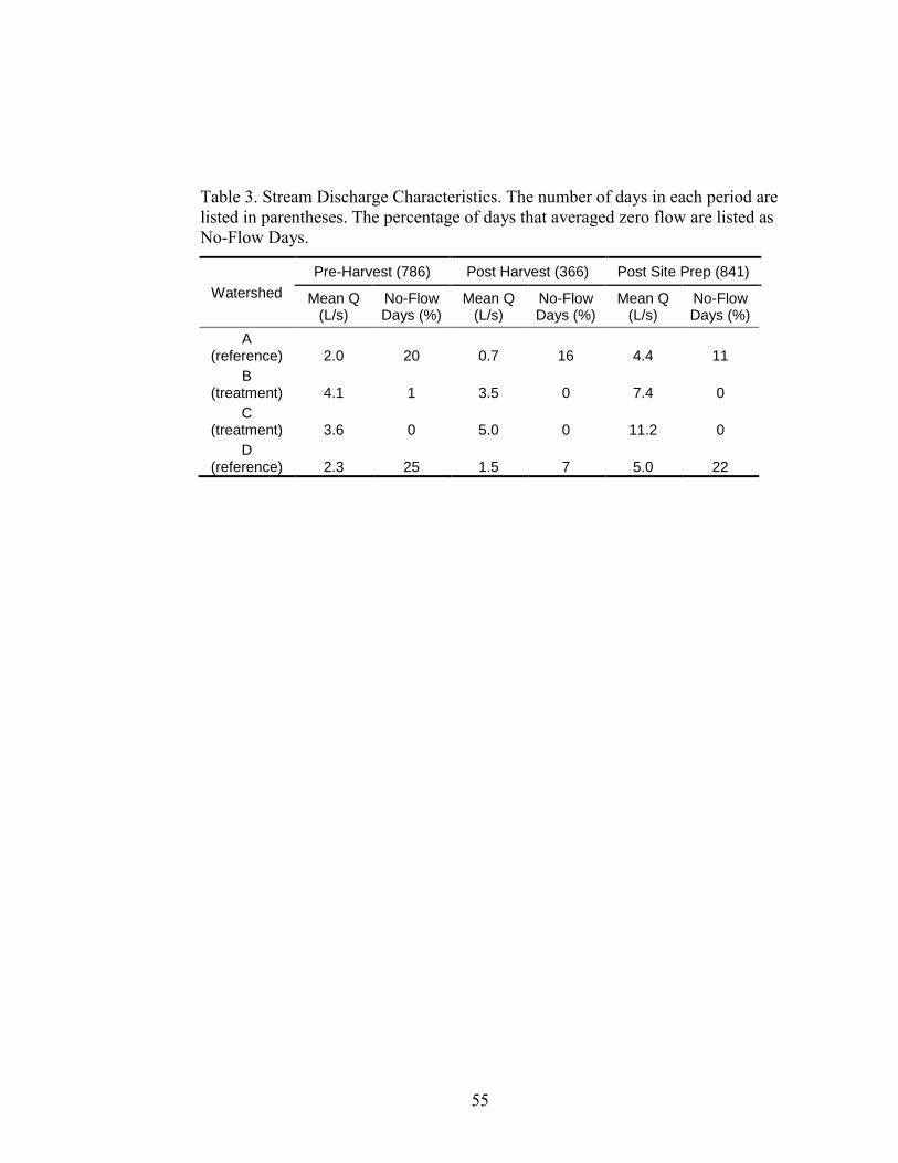
55

Table 3. Stream Discharge Characteristics. The number of days in each period are listed in parentheses. The percentage of days that averaged zero flow are listed as No-Flow Days.

Watershed

Pre-Harvest (786) Post Harvest (366) Post Site Prep (841)

Mean Q (L/s)

No-Flow Days (%)

Mean Q (L/s)

No-Flow Days (%)

Mean Q (L/s)

No-Flow Days (%)

A (reference) 2.0 20 0.7 16 4.4 11

B (treatment) 4.1 1 3.5 0 7.4 0

C (treatment) 3.6 0 5.0 0 11.2 0

D (reference) 2.3 25 1.5 7 5.0 22

56

Table 4. Summary of Double Mass Curves. Changes in treatment water yield during the post harvest and post site preparation period compared to the pre-harvest relationship with the corresponding reference watershed.

Watershed

B B C C

(vs. A) (vs. D) (vs. A) (vs. D)

Post Harvest

Increase (%) 150 30 315 117

Increase (mm) 208 79 289 205

Error (+/-) 4 8 3 5

Post Site Preparation

Increase (%) -19 -16 39 45

Increase (mm) -381 -315 521 573

Error (+/-) 43 42 28 27

57

Table 5. Mean suspended sediment yield for all watersheds during the pre-harvest, post harvest, and post site preparation. Pair-wise comparisons were done by year.

Mean Sediment Yield (kg/ha/yr)

Watershed Year 1 (pre)

Year 2 (pre)

Year 3 (post)

Year 4 (psp)

Year 5 (psp)

A (reference)

18.7a* 62.0a 37.4a 74.3a 41.8a

B (treatment)

116.8b 115.4a 79.7a 173.7a 65.5a

C (treatment)

71.4ab 699.5b 289.3b 1255.0b 276.9a

D (reference)

36.4ab 859.5c 179.5b 341.6b 71.5a

* Means followed by the same letter are not significantly different (P ≤ 0.05).

58

Table 6. Breakthrough Survey. The average number of pre-harvest and post harvest period breakthroughs listed by watershed and categorized by breakthrough type.

Watershed Flow and

Sediment enter stream (pre/post)

Flow enters stream

(pre/post)

Flow enters SMZ, but stopped (pre/post)

A (reference) 0 / 0 0 / 1 0 / 2

D (reference) 0 / 0 0 / 6 0 / 6

B (treatment) 0 / 0 0 / 6 1 / 6

C (treatment) 1 / 3 1 / 10 2 / 21

59

Table 7. Breakthrough Sources. Post harvest breakthrough survey results for the treatment watersheds. The number of recorded breakthroughs are listed by source and categorized by field observations.

Breakthrough Source Flow and Sediment enter stream

Flow enters stream

Flow enters SMZ, but stopped

Fire Break 16 24 81

Seep 0 38 28

Planar Slope 1 8 32

Swale 1 5 9

Gullies 0 4 2

60

Table 8. Average bare mineral soil as a percentage of watershed area for the pre-harvest, post harvest, and post site preparation periods. Watersheds A and D are reference watersheds B and C are treatment watersheds. The number of random plots per watershed are in parentheses.

A (84) B (96) C (120) D (132)

2002 (pre) 2.4 1.6 2.3 2.5

2003 (pre) 3.9 2.8 2.5 4.6

2004 (post) 3.5 8.1 16.1 5.6

2006 (psp) 0.6 8.9 12.3 0.2

61

Table 9. Vegetation Survey (understory groundcover). Average understory vegetation cover as a percentage of watershed area for the pre-harvest, post harvest, and post site preparation periods. Watersheds A and D are reference watersheds B and C are treatment watersheds. The number of random plots per watershed are in parentheses.

A (84) B (96) C (120) D (132)

2002 (pre) 19.1 17.2 18.1 13.4

2003 (pre) 18.9 17.2 17.8 9.5

2004 (post) 23.2 38.7 37.2 10.9

2006 (psp) 22.8 37.3 37.7 10.3

62

Figu

re 1

. Dry

Cre

ek S

tudy

Loc

atio

n (3

0°4

7’3

0’N

and 8

4°3

7’3

0W

). Lo

catio

ns o

f the

four

exp

erim

enta

l w

ater

shed

s, sa

mpl

ing

and

data

reco

rdin

g si

tes a

re in

dica

ted

with

in th

e m

ain

win

dow

of t

he fi

gure

. Gen

eral

lo

catio

n an

d po

st h

arve

st a

eria

l pho

togr

aphs

of t

he tr

eatm

ent w

ater

shed

s are

loca

ted

in th

e sm

alle

r win

dow

s of

the

figur

e. BB B

C

63

Date

Jan-01 Jul-01 Jan-02 Jul-02 Jan-03 Jul-03 Jan-04 Jul-04 Jan-05 Jul-05 Jan-06 Jul-06 Jan-07 Jul-07

Cum

ula

tive R

ain

fall

(mm

)

0

2000

4000

6000

8000

Year 1772 mm

Year 21270 mm

Year 41702 mm

Year 31358 mm

Year 5976 mm

Harv

est

773 m

m

Figure 2. Cumulative Precipitation. Data from Class A weather station located between watersheds C and D of the Dry Creek watershed study.

64

Flow Exceedence Percentage

0.1 1 10 100

Flo

w (

L/s

)

0

50

100

150

200

250

300

350

A (Pre)

B (Pre)

Col 9 vs A (L/s)

Col 9 vs Col 11

Figure 3. Flow Distribution (WS A and B). Pre-harvest and post harvest flow distribution for watersheds A (reference) and B (treatment).

65

Flow Exceedence Percentage

0.1 1 10 100

Flo

w (

L/s

)

0

50

100

150

200

250

300

350

C (Pre)

D (Pre)

Col 9 vs Col 12

Col 9 vs Col 13

Figure 4. Flow Distribution (WS C and D). Pre-harvest and post harvest flow distribution for watersheds C (treatment) and D (reference).

66

Yr 1 Yr 2 Yr 3 Yr 4 Yr 5

Wate

r Y

ield

(m

m)

0

200

400

600

800

1000

1200

1400

1600

1800

2000

A

B

C

D

Rainfall

Figure 5. Annual Water Yield. Depth of precipitation was recorded from the weather station between watersheds C and D.

67

2001 2002 2003 2004 2005 2006 2007 2008

Cu

mu

lative

Ru

no

ff W

S A

, B

, C

an

d D

(m

m)

0

500

1000

1500

2000

2500

3000

WS A

WS B

WS C

WS D

Harv

est

Site

Pre

pa

ratio

n

Figure 6. Cumulative Water Yield.

68

Cumulative Runoff WS A (mm)

0 200 400 600 800 1000 1200 1400 1600 1800

Cu

mu

lative

Ru

no

ff W

S B

, C

an

d D

(m

m)

0

500

1000

1500

2000

2500

3000

WS B

WS C

WS D

Ha

rve

st

Site

Pre

pa

ratio

n

Figure 7. Double Mass Curves (vs. WS A). Double mass curves of cumulative runoff (mm). The cumulative flow during the harvest period for watershed A was low, which gives the appearance of only one line.

69

Cumulative Runoff WS D (mm)

0 250 500 750 1000 1250

Cum

ula

tive R

un

off W

S A

, B

and

C (

mm

)

0

500

1000

1500

2000

2500

3000

WS B

WS C

WS A

Harv

est

Site P

rep

ara

tion

Figure 8. Double Mass Curves (vs. WS D).

70

Figure 9. Dunne and Leopold (1978). First year increases in water yield as a function of percentage of vegetation removed. Watershed B has open symbols and watershed C has closed symbols. Circles correspond to treatment watersheds versus WS A and squares correspond to treatment watersheds versus WS D. Data from double mass curves. Figure from Dunne and Leopold (1978).

WS C WS B

71

Log Peakflow WS A (L/s)

0 1 2 3 4 5

Log P

eakflow

WS

B (

L/s

)

0

1

2

3

4

5

Pre (measured)

Post (measured)

Pre (estimated)

Post (estimated)

USGS 2-, 10-, 100-yr Flood

Pre-harvest Regression

Post Harvest regression

Figure 10. Peakflow Regression (WS A and B). Log transformed pre-harvest and post harvest peakflow regressions for watersheds A (reference) and B (treatment).

72

Log Peakflow WS D (L/s)

0 1 2 3 4 5

Lo

g P

ea

kflo

w W

S C

(L

/s)

0

1

2

3

4

5

Pre (measured)

Post (measured)

Pre (estimated)

Post (estimated)

USGS 2-, 10-, 100-yr Flood

Pre-harvest Regression

Post Harvest Regression

Figure 11. Peakflow Regression (WS C and D). Log transformed pre-harvest and post harvest peakflow regressions for watersheds C (treatment) and D (reference).

73

Year 1

A1 B1 C1 D1

Diu

rna

l F

low

Am

plit

ud

e (

L/s

)

0

1

2

3

4

5

Year 2

A1 B1 C1 D1

Diu

rna

l F

low

Am

plit

ud

e (

L/s

)

0

1

2

3

4

5

Year 3

A1 B1 C1 D1

Diu

rna

l F

low

Am

plit

ud

e (

L/s

)

0

1

2

3

4

5

Year 4

A1 B1 C1 D1

Diu

rna

l F

low

Am

plit

ud

e (

L/s

)

0

1

2

3

4

5

6

7

Year 5

A1 B1 C1 D1

Diu

rna

l F

low

Am

plit

ud

e (

L/s

)

0

1

2

3

4

5

Figure 12. Diurnal Flow Amplitudes. Box plots of diurnal flow amplitude for each year.

74

Yr 1 Yr 2 Yr 3 Yr 4 Yr 5

To

tal S

usp

en

de

d S

olid

Yie

ld (

kg/h

a)

0

200

400

600

800

1000

1200

1400

A

B

C

D

Figure 13. Annual Total Suspended Solid Yield.

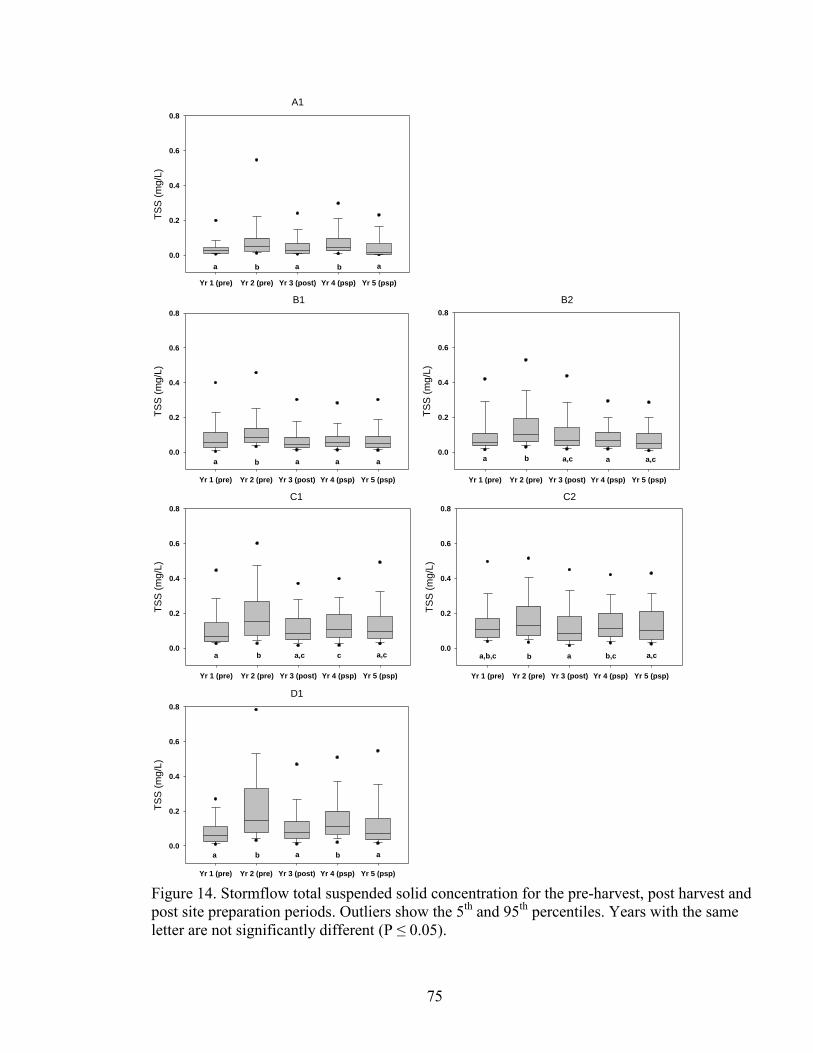
75

A1

Yr 1 (pre) Yr 2 (pre) Yr 3 (post) Yr 4 (psp) Yr 5 (psp)

TS

S (

mg/L

)

0.0

0.2

0.4

0.6

0.8

a b a b a

B1

Yr 1 (pre) Yr 2 (pre) Yr 3 (post) Yr 4 (psp) Yr 5 (psp)

TS

S (

mg/L

)

0.0

0.2

0.4

0.6

0.8

a b a a a

B2

Yr 1 (pre) Yr 2 (pre) Yr 3 (post) Yr 4 (psp) Yr 5 (psp)

TS

S (

mg/L

)

0.0

0.2

0.4

0.6

0.8

a a,c a a,cb

C1

Yr 1 (pre) Yr 2 (pre) Yr 3 (post) Yr 4 (psp) Yr 5 (psp)

TS

S (

mg/L

)

0.0

0.2

0.4

0.6

0.8

a a,c a,cb c

C2

Yr 1 (pre) Yr 2 (pre) Yr 3 (post) Yr 4 (psp) Yr 5 (psp)

TS

S (

mg

/L)

0.0

0.2

0.4

0.6

0.8

a,b,c b a b,c a,c

D1

Yr 1 (pre) Yr 2 (pre) Yr 3 (post) Yr 4 (psp) Yr 5 (psp)

TS

S (

mg/L

)

0.0

0.2

0.4

0.6

0.8

a b a b a

Figure 14. Stormflow total suspended solid concentration for the pre-harvest, post harvest and post site preparation periods. Outliers show the 5th and 95th percentiles. Years with the same letter are not significantly different (P ≤ 0.05).

76

Water Yield (mm)

0 200 400 600 800 1000 1200

TS

S Y

ield

(kg/h

a)

0

50

100

150

200

250

300

Year 1 (Pre)

Year 2 (Pre)

Year 3 (Post)

Year 4 (Post)

Year 5 (Post)

WS A (open)

WS B (closed)

Figure 15. TSS Yield vs. Water Yield (WS A and B). Total suspended solid and annual water yield relationships for watersheds A (reference) and B (treatment).

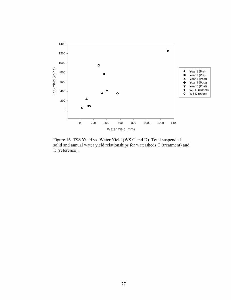
77

Water Yield (mm)

0 200 400 600 800 1000 1200 1400

TS

S Y

ield

(kg/h

a)

0

200

400

600

800

1000

1200

1400

Year 1 (Pre)

Year 2 (Pre)

Year 3 (Post)

Year 4 (Post)

Year 5 (Post)

WS C (closed)

WS D (open)

Figure 16. TSS Yield vs. Water Yield (WS C and D). Total suspended solid and annual water yield relationships for watersheds C (treatment) and D (reference).

78

A1

Flow (L/s)

0.001 0.01 0.1 1 10 100 1000 10000

TS

S (

mg

/L)

0.1

1

10

100

1000

10000

B1

Flow (L/s)

0.1 1 10 100 1000 10000

TS

S (

mg

/L)

0.1

1

10

100

1000

10000

C1

Flow (L/s)

0.1 1 10 100 1000

TS

S (

mg/L

)

1

10

100

1000

10000

D1

Flow (L/s)

0.01 0.1 1 10 100 1000

TS

S (

mg

/L)

1

10

100

1000

10000

Figure 17. C - Q Relationship. Total suspended solid concentration and stream discharge relationships for all watersheds.

79

Clockwise

Flow (L/s)

4 6 8 10 12 14 16 18

TS

S (

mg

/L)

0

20

40

60

80

100

120

No Pattern

Flow (L/s)

14.0 14.5 15.0 15.5 16.0 16.5 17.0

TS

S (

mg

/L)

2.5

3.0

3.5

4.0

4.5

5.0

5.5

Figure Eight

Flow (L/s)

0 10 20 30 40 50 60

TS

S (

mg

/L)

0

100

200

300

400

500

600

700

800

Straight Line

Flow (L/s)

0 20 40 60 80 100

TS

S (

mg/L

)

0

200

400

600

800

1000

Figure 18. Hysteresis Examples. Examples of observed single event suspended sediment hysteresis patterns.

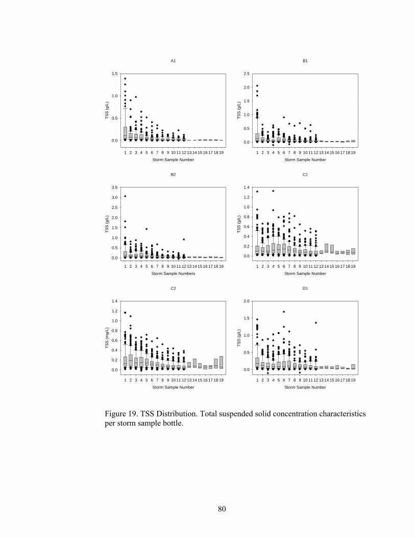
80

A1

Storm Sample Number

1 2 3 4 5 6 7 8 9 10 11 12 13 14 15 16 17 18 19

TS

S (

g/L

)

0.0

0.5

1.0

1.5

B1

Storm Sample Number

1 2 3 4 5 6 7 8 9 10 11 12 13 14 15 16 17 18 19

TS

S (

g/L

)

0.5

1.5

2.5

0.0

1.0

2.0

B2

Storm Sample Numbers

1 2 3 4 5 6 7 8 9 10 11 12 13 14 15 16 17 18 19

TS

S (

g/L

)

0.0

0.5

1.0

1.5

2.0

2.5

3.0

3.5

C1

Storm Sample Number

1 2 3 4 5 6 7 8 9 10 11 12 13 14 15 16 17 18 19

TS

S (

g/L

)

0.0

0.2

0.4

0.6

0.8

1.0

1.2

1.4

C2

Storm Sample Number

1 2 3 4 5 6 7 8 9 10 11 12 13 14 15 16 17 18 19

TS

S (

mg

/L)

0.0

0.2

0.4

0.6

0.8

1.0

1.2

1.4

D1

Storm Sample Number

1 2 3 4 5 6 7 8 9 10 11 12 13 14 15 16 17 18 19

TS

S (

g/L

)

0.0

0.5

1.0

1.5

2.0

Figure 19. TSS Distribution. Total suspended solid concentration characteristics per storm sample bottle.