Hydrogen Sulfide Mitigation Strategy for a Class I Landfill

Submitted by

Kevin Kung (kkung@mit.edu)

Rajesh Sridhar (srajesh@mit.edu)

Heather Yang (hjy@mit.edu)

Massachusetts Institute of Technology (MIT)

July 15, 2015

TABLE OF CONTENTS

1. Introduction ……………………………… 1

2. Assumptions and Data Analysis ………… 4

3. Technology Review ……………………... 10

4. Technical Comparison …………………... 15

5. Economic Comparison …………………... 20

6. Conclusion and Recommendations ……… 25

7. References ……………………………….. 30

8. Figures …………………………………… 31

9. Tables ……………………………………. 36

1

1. INTRODUCTION

1.1 Background

This report concerns the need for H2S mitigation in a Class I landfill, operated by the Solid

Waste Department of Hottenhumid County, Florida. Since its inception, the landfill has been

receiving unprocessed municipal waste and fly ash from a nearby waste-to-energy and the

landfill gas generated from these waste was collected and processed onsite for use as fuel.

However, over the last few years, the landfill had also been accepting construction and

demolition (C&D) waste from a recycling facility. Recently, there has been a drastic increase in

the hydrogen sulfide (H2S) concentrations (of up to 3000 ppmv) in the landfill gas (LFG),

possibly due to the gypsum-containing C&D waste. Since the end of 2014, the landfill stopped

accepting C&D waste, but the unacceptably high H2S levels remain, and may take years to

mitigate. The county has determined that an H2S limit of 300 ppm is required (due to the

associated post-combustion SO2/SO3 emission limits). To accomplish this target, it becomes

necessary to install an on-site H2S removal facility. This report predicts the future unmitigated

H2S emissions in the LFG, assesses the different H2S removal technologies to help the county

achieve the target H2S limit, and makes a recommendation for a path forward.

1.2 Rationale of Our Approach

In this section, we give a general description of the key data available to us from the landfill, as

well as an overview of our approach for techno-economic assessment. The criteria for evaluating

the different H2S removal technologies can be broadly classified as technical and economic.

While economics forms the core of the non-technical considerations, the technical criteria

involves the capability of the technology to operate efficiently under the given operating

2

conditions such as the landfill gas flow rate and the associated H2S concentrations. This led us to

first seek to accurately predict the flow rate of collected LFG flow rate and H2S concentrations in

the future, so that we can identify technologies that are compatible with these technical

requirements.

1.2.1 Historical Data

The early part of this work discusses the methodology and the various assumptions associated

with modeling the H2S concentrations and the LFG flow rates. Based on existing models, we

developed a simple first-order kinetic description to predict the H2S and LFG generation rates.

While some of the model parameters were taken from the literature, the other parameters were

calculated based on the available information and the observed values. To help us with our

modeling effort, the county has provided us with some historical data on (a) LFG flow rate and

(b) H2S concentration in the LFG.

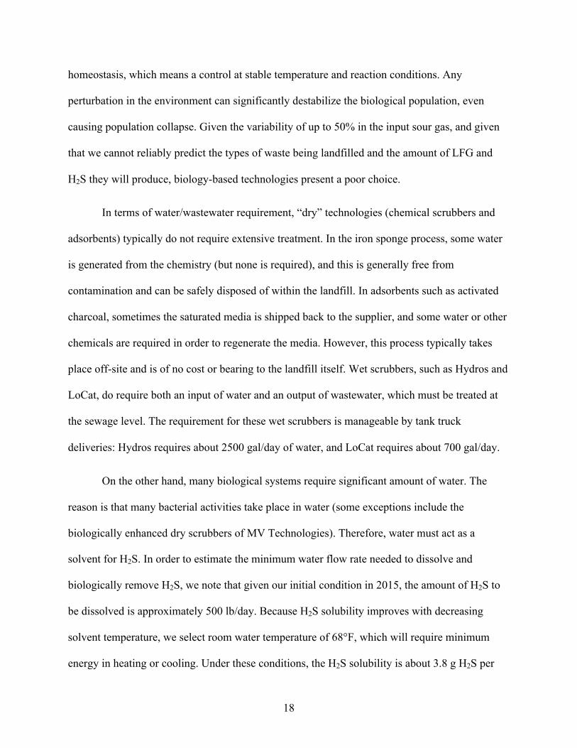
Fig. 1 shows the historical LFG collected at the landfill. From 2009 to mid-2013, the

level is variable but generally steady at about 1200 scfm. Starting in July 2013, there is a drastic

increase in the LFG collected. This is due to a combination of increased waste being landfilled

during this period (see Fig. 2), as well as an improvement in the LFG collection efficiency,

according to our client.

Fig. 2 shows the historical H2S concentration and its correlation with C&D debris data at

this landfill. As we can see, the landfill began accepting C&D waste in July 2012, and ceased by

January 2015. During this period, the H2S concentration in the LFG has drastically increased

from about 200 ppmv to more than 3000 ppmv.

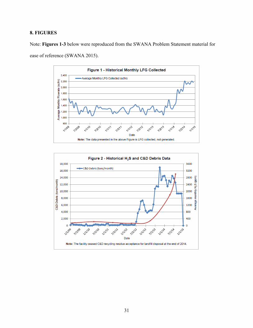
1.2.2 Landfill Projections

3

Based on Figs. 1-2, it is possible for us to extract key correlations between the amount of

waste being landfilled (non-C&D and C&D wastes), and the LFG/H2S production rate. However,

in order to help us predict the future levels, it is also necessary for the landfill to provide us with

projected waste landfilled (both ash and non-ash wastes), as Fig. 3 illustrates. In this figure, we

note that the landfill is expected to be in operation until 2046. In the long-term future, there is a

steady increase in the total waste landfilled from year to year. Qualitatively, we expect the LFG

collected to also increase, assuming that the nature of the waste remains constant. However, in

the short-term future (2015-2016), we noticed a sudden departure from historical trend. Namely,

the total waste landfilled almost halves, while the amount of ash landfilled almost tripled.

According to the landfill, this is due to a new waste-to-energy expansion at the landfill. A larger

fraction of the waste traditionally landfilled would instead be incinerated, yielding a larger

amount of ash, which is consistent with the projected data.

1.2.3 Technical Assessment

We first identified various broad classes of H2S removal technologies, and then evaluated

their suitability based on specific technical requirements imposed by our prior modeling

predictions. This includes factors such as robustness against input variability, water

requirements, and waste disposal requirements. Some classes of technologies are ruled out at this

stage, allowing us to hone in a few technologies represented by selected companies.

1.2.4 Economic Assessment

Once we have honed in on specific technologies to consider, we discussed our detailed

requirements with the individual companies, and obtained quotations from them. This gave us a

basis for calculating and comparing the economic performance of each technology.

4

2. ASSUMPTIONS AND DATA ANALYSIS

2.1 Assumptions

• LFG consists, on molar basis, of 50% methane, 33% carbon dioxide, 2% oxygen at 122°F.

The remainder consists mostly of water vapor, and trace gases such as H2S.

• We ignored other sulfur impurities such as carbonyl sulfide, carbon disulfide, and other

organic sulfur compounds which may contribute to the total sulfur due to C&D waste.

• Beyond changes in H2S levels, the introduction of C&D waste did not drastically change the

overall LFG composition. We also assumed that C&D waste exhibits similar landfill gas

emission characteristics as the unprocessed municipal waste.

• The C&D waste contains about 20% gypsum by mass (Gp = 0.2). Of the gypsum, about 18%

by mass is sulfur (Sg = 0.18) and will be released as H2S.

• The waste streams consist solely of ash, putrescible waste, and C&D waste. Other potential

streams, such as plastics, metals, etc. are assumed to be recycled perfectly at an earlier step.

• Gas pressure was assumed to be about 28 inches of water column.

• It will take a minimum 12 weeks from the report’s date to set up/commission the technology.

Thus, the system was sized to handle 150% of the maximum H2S levels at/after Oct. 2015.

• Given an H2S emission ceiling of 300 ppmv, we set the design target for output H2S level to

be 50% of that value, or 250 ppmv. The H2S removal technology is no longer needed when

the mean H2S level in the LFG falls below 250 ppmv for 3 consecutive months.

• This landfill, like some other landfills, does not readily have a large source of water or

wastewater disposal (e.g. sewage) facility. Water /wastewater transport requires trucks.

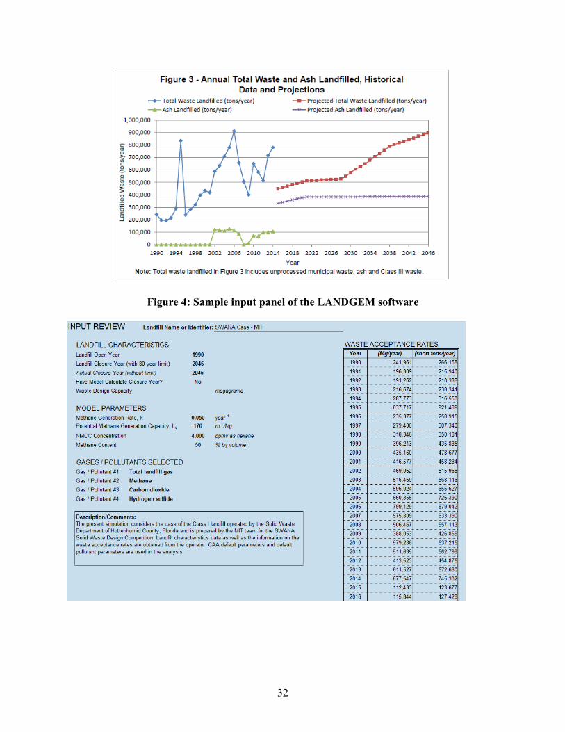
2.2 Landfill Gas Collection Prediction Using LANDGEM

5

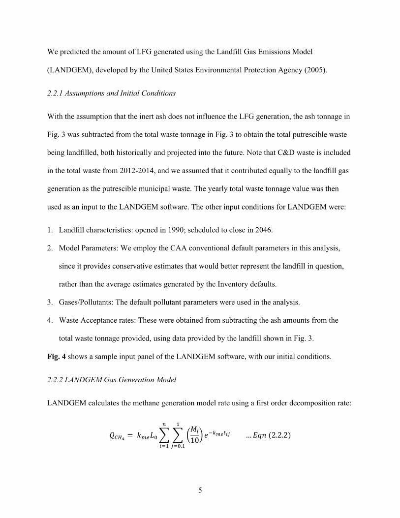
We predicted the amount of LFG generated using the Landfill Gas Emissions Model

(LANDGEM), developed by the United States Environmental Protection Agency (2005).

2.2.1 Assumptions and Initial Conditions

With the assumption that the inert ash does not influence the LFG generation, the ash tonnage in

Fig. 3 was subtracted from the total waste tonnage in Fig. 3 to obtain the total putrescible waste

being landfilled, both historically and projected into the future. Note that C&D waste is included

in the total waste from 2012-2014, and we assumed that it contributed equally to the landfill gas

generation as the putrescible municipal waste. The yearly total waste tonnage value was then

used as an input to the LANDGEM software. The other input conditions for LANDGEM were:

1. Landfill characteristics: opened in 1990; scheduled to close in 2046.

2. Model Parameters: We employ the CAA conventional default parameters in this analysis,

since it provides conservative estimates that would better represent the landfill in question,

rather than the average estimates generated by the Inventory defaults.

3. Gases/Pollutants: The default pollutant parameters were used in the analysis.

4. Waste Acceptance rates: These were obtained from subtracting the ash amounts from the

total waste tonnage provided, using data provided by the landfill shown in Fig. 3.

Fig. 4 shows a sample input panel of the LANDGEM software, with our initial conditions.

2.2.2 LANDGEM Gas Generation Model

LANDGEM calculates the methane generation model rate using a first order decomposition rate:

!!"! = !!!"!!!!10 !!!!"!!"

!

!!!.!!!!!!!!!…!"#!(2.2.2)

!

!!!

6

where !!"! is the annual methane generation (m3/year), kme is the methane generation rate (in

year-1) and !! is the potential methane generation capacity (m3/Mg), !! is the amount of waste

(Mg) accepted in the year i, n is the running residence time of the waste in the landfill at year j

(current calculation), and !!" is the age of the jth section of waste Mi. The summation relates to the

fact that various segments of the landfill are laid down at different points (i) in time, and over a

time period j will release certain amounts of CH4. The various parameters L0 and kme are already

built into the LANDGEM model using the initial conditions described in the previous section, so

given the input Mi from the landfill data (Fig. 3), we are able to predict !!"!.

In order to relate !!"! to the overall LFG flow rate QLFG, we utilized our assumption that

the CH4 molar fraction in our landfill’s LFG is !!"! = 50%. Thus, !!"# = !!"!/!!!!.

2.2.3 Landfill Gas Collection Model

The predicted LFG flow rate QLFG from the LANDGEM model determine only the amount of

landfill gas generated, but depending on the landfill design, not all generated gas can be

collected. There is a factor Fc that describes the collection efficiency—that is, the fraction of LFG

generated that is actually collected. The LANDGEM model tells us nothing about this collection

efficiency, which we will have to infer from our existing data (Fig. 1, Fig. 3) by curve-fitting.

Defining the total collected LFG flow rate as QLFGC, our fit function is given as follows:

!!"#$ = !!!!"# !!!!!!…!"#! 2.2.3 .

On the left-hand side, QLFGC is derived from interpolating Fig. 1 (using monthly data

interpolation). On the right-hand side, QLFG is calculated by applying the LANDGEM model to

Fig. 3 (also using monthly data interpolation). This gives us a way to find the fitting parameter

7

Fc that minimizes the least squares of the problem above. Another confounding factor is that in

the latter half of 2013, improvements to the landfill facilities increased the collection efficiency

Fc. Therefore, we need to split the fitting into two segments with different Fc values: a pre-2013

phase where Fc is lower, and a post-2013 phase where Fc is higher.

As an example, for data before 2013, this Fc value was fitted to be 0.19, which forms the

Base Case of our scenario. However, we have noticed in Fig. 1 that the LFG flow rate can

fluctuate from month to month; thus, due to the random fluctuations in Fig. 1, the actual value of

Fc could be larger or smaller. To estimate how large this uncertainty range is, we calculated the

standard deviation of the data σLFG (i.e. how spread out the fluctuation in Fig. 1 is). Assuming

that the observed fluctuation is roughly Gaussian, we can calculate the 95% confidence interval

as ±1.96!!"#/ !, where N is the number of data points (sample size). Let us define the upper

and lower bounds of our 95% confidence interval the “Optimistic Case” (with a higher collection

efficiency), and “Conservative Case” (with a slightly lower collection efficiency).

The fitted values for Fc are summarized in Table 1 for the different scenarios. We carried

out similar calculations for the post-2014 data (after improvements were made to gas collection).

We see that during 2014, there was a ~12-15% improvement in gas collection efficiency.

2.2.4 Predicting Future LFG Generation

Based on the LANDGEM model and fitting for the gas collection efficiency, we have enough

information to predict the future flow rates of collected LFG. The overall fitted LFG historical

data and inferred future predictions calculated using the three Cases (Base, Optimistic, and

Conservative) are plotted in Fig. 5. We first observed a sharp increase around 2015 in the

collected LFG. This replicates the sharp increase described in Fig. 1 due to the increase in LFG

8

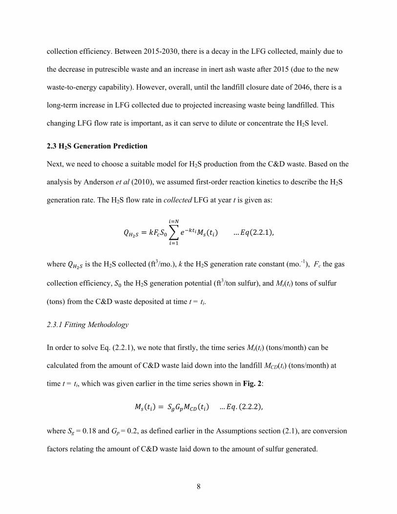
collection efficiency. Between 2015-2030, there is a decay in the LFG collected, mainly due to

the decrease in putrescible waste and an increase in inert ash waste after 2015 (due to the new

waste-to-energy capability). However, overall, until the landfill closure date of 2046, there is a

long-term increase in LFG collected due to projected increasing waste being landfilled. This

changing LFG flow rate is important, as it can serve to dilute or concentrate the H2S level.

2.3 H2S Generation Prediction

Next, we need to choose a suitable model for H2S production from the C&D waste. Based on the

analysis by Anderson et al (2010), we assumed first-order reaction kinetics to describe the H2S

generation rate. The H2S flow rate in collected LFG at year t is given as:

!!!! = !!!!! !!!!!!!(!!!!!

!!!) !!!!!!!!…!" 2.2.1 ,

where !!!! is the H2S collected (ft3/mo.), k the H2S generation rate constant (mo.-1), Fc the gas

collection efficiency, !! the H2S generation potential (ft3/ton sulfur), and Ms(ti) tons of sulfur

(tons) from the C&D waste deposited at time t = ti.

2.3.1 Fitting Methodology

In order to solve Eq. (2.2.1), we note that firstly, the time series Ms(ti) (tons/month) can be

calculated from the amount of C&D waste laid down into the landfill MCD(ti) (tons/month) at

time t = ti, which was given earlier in the time series shown in Fig. 2:

!! !! = !!!!!!!" !! !!!!!…!". 2.2.2 ,

where Sg = 0.18 and Gp = 0.2, as defined earlier in the Assumptions section (2.1), are conversion

factors relating the amount of C&D waste laid down to the amount of sulfur generated.

9

Next, k describes how quickly H2S is released from its store. k is estimated based on

empirical data from 6 landfills reported in Anderson et al (2010). These curve-fitted k values are

quite variable, so we took the mean ! of the 6 k values as our “Base Case” scenario, which

turned out to be 0.64 months-1. We also calculated the standard deviation σk around the mean.

Assuming a Gaussian distribution, we can then define our upper and lower bounds of the 95%

confidence interval for the value k as ! ± 1.96!!!/ !, where N = 6 is the sample size. In our

case, the 95% confidence interval around 0.64 months-1 was found to be ±0.14 months-1. In other

words, we can be fairly confident (95% of the time) that the actual k value for our Florida landfill

will be between the upper bound of ! + 1.96!!!/ ! = 0.78 months-1 (“Optimistic Case”, the

H2S levels decay more quickly) and lower bound of ! − 1.96!!!/ ! = 0.50 months-1

(“Conservative Case”). Table 2 shows these data and how we derived the k value in detail.

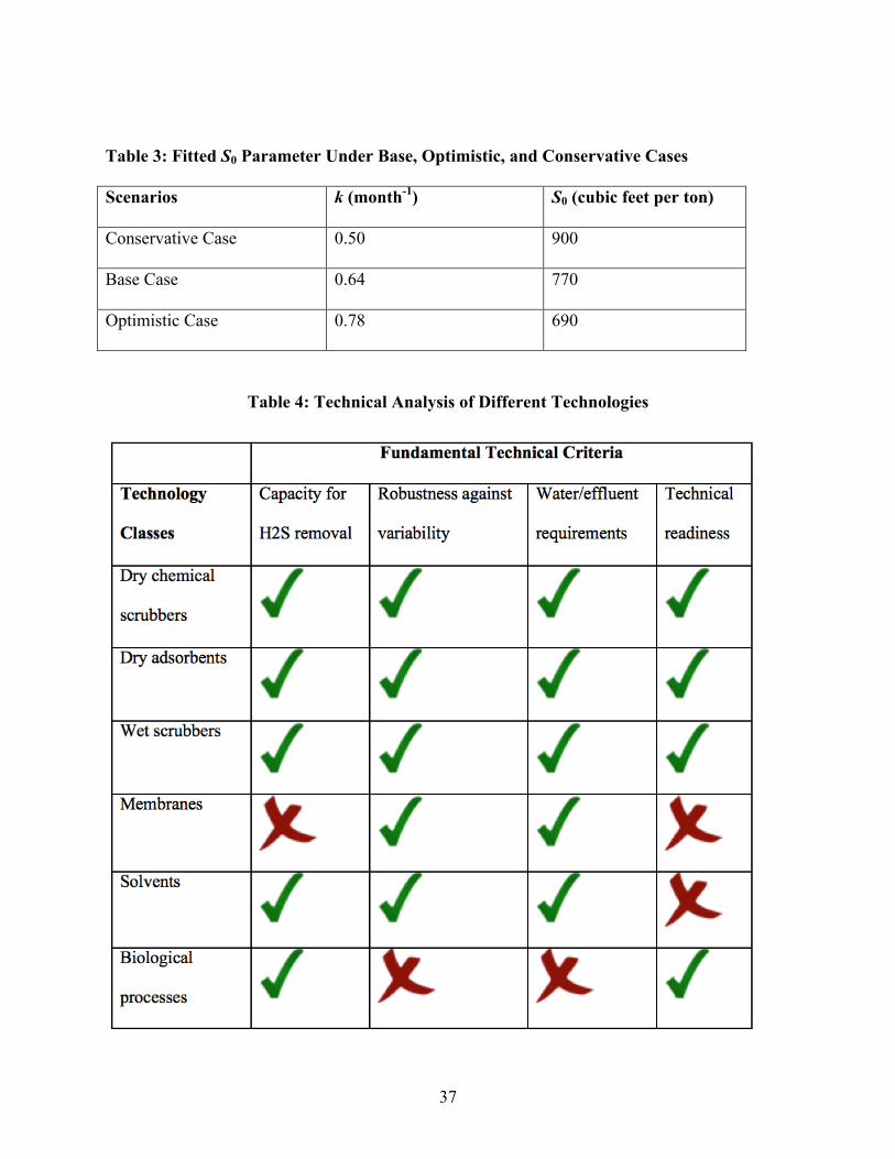
Given Ms(ti) and a range of likely k values, we can then define S0 (H2S generation

potential) in Eqn. (2.2.1) to be our fitting parameter, such that the predicted !!!!, when

converted into H2S concentration (in ppmv) by dividing into the LFG flow rate, has the best

least-squared fit with the actual H2S flow rate measured by the landfill in Fig. 2. In other words,

we carried out 3 separate sets of data fitting for “Base Case”, “Optimistic Case”, and

“Conservative Case”, and found the S0 parameter in each case that would optimize the least-

squared fit. These different values of S0, summarized in Table 3 for the different Cases, then also

define the Base Case and the upper and lower bounds of the 95% confidence interval range.

Fig. 6 shows the predicted H2S level (ppmv). We see initially a rapid rise to 3000-5000

ppmv, but as soon as C&D collection ceases, the H2S level drops exponentially. In general, the

H2S will return to pre-2012 level by the year 2021, which means that H2S removal technology is

needed for at least 6 years.

10

3. TECHNOLOGY REVIEW

H2S removal technologies have been roughly classified into five main categories. In this section,

we explain how each mechanism of H2S removal functions in each category and identity the

strengths and weaknesses of each class of technology.

3.1. Dry Processes

Dry chemical processes are the most competitive on capital and media costs and remain the

archetypical choice for biogas purification (Zicari 2003). These processes are work by the

reaction between the H2S gas and a solid chemical catalyst or adsorbent. In general, these

technologies utilize replaceable dry media to extract H2S until the media becomes saturated and

needs to be replaced. The typical design is for there to be two separate reaction vessels, such that

if one vessel goes off-line (e.g. media replacement), the H2S scrubbing is not interrupted.

The reaction types are wide-ranging, but they can be classified into three sub-categories: 1)

Metal oxides (e.g., SulfaTreat, Sulfur-Rite, Media G-2, Puraspec); 2) Alkaline solids (Sofnolime-

RG); and 3) Adsorbents. We will discuss the more popular categories 1 and 3 in depth.

3.1.1 Metal oxides (sponges)

In metal oxide technologies, the metal acts as a catalyst to convert H2S into elemental sulfur. The

following is an example of the “iron sponge” reaction:

Fe2O3 + 3H2S ! Fe2S3 + 3H2O; Fe2S3 + O2 ! 2Fe2O3 + 3S2.

In this case, the source of O2 comes from the landfill gas, and the byproduct is non-contaminated

water. SulfaTreat, MV Technologies, and BioREM all have technologies that are in this space. In

11

particular, SulfaTreat uses a proprietary granulated support structure for the media. MV

Technologies couples the iron sponge concept with a biological iron re-oxidation step.

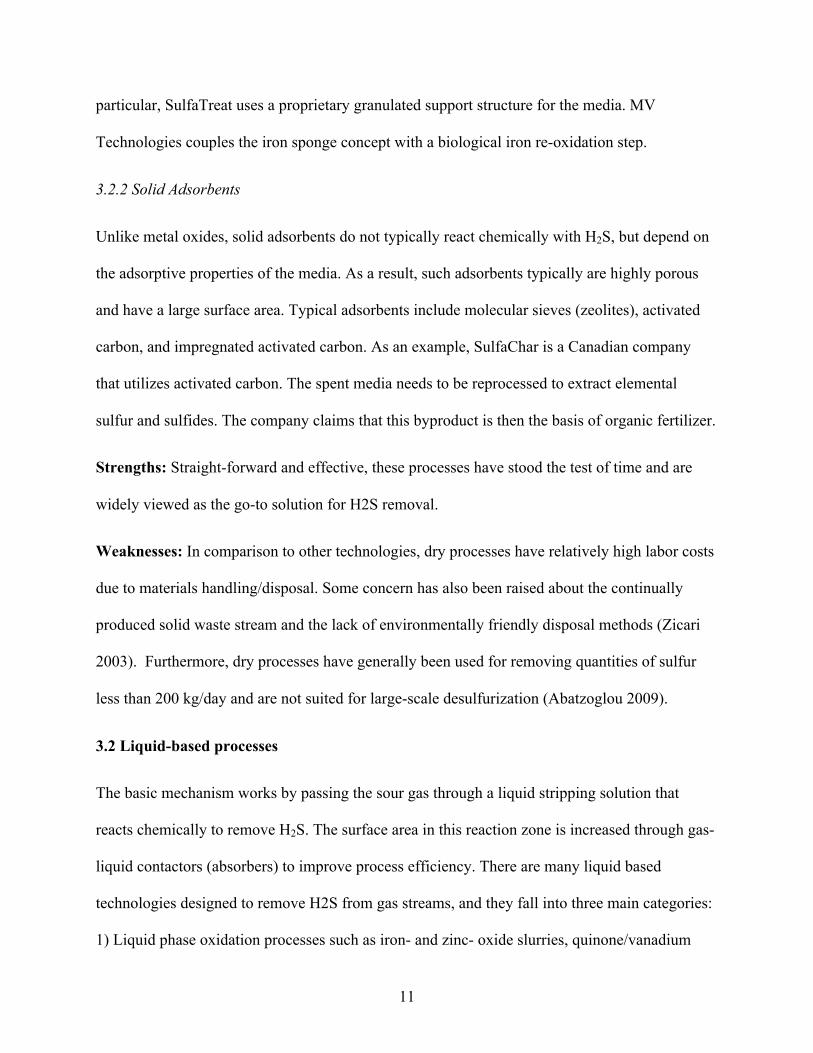
3.2.2 Solid Adsorbents

Unlike metal oxides, solid adsorbents do not typically react chemically with H2S, but depend on

the adsorptive properties of the media. As a result, such adsorbents typically are highly porous

and have a large surface area. Typical adsorbents include molecular sieves (zeolites), activated

carbon, and impregnated activated carbon. As an example, SulfaChar is a Canadian company

that utilizes activated carbon. The spent media needs to be reprocessed to extract elemental

sulfur and sulfides. The company claims that this byproduct is then the basis of organic fertilizer.

Strengths: Straight-forward and effective, these processes have stood the test of time and are

widely viewed as the go-to solution for H2S removal.

Weaknesses: In comparison to other technologies, dry processes have relatively high labor costs

due to materials handling/disposal. Some concern has also been raised about the continually

produced solid waste stream and the lack of environmentally friendly disposal methods (Zicari

2003). Furthermore, dry processes have generally been used for removing quantities of sulfur

less than 200 kg/day and are not suited for large-scale desulfurization (Abatzoglou 2009).

3.2 Liquid-based processes

The basic mechanism works by passing the sour gas through a liquid stripping solution that

reacts chemically to remove H2S. The surface area in this reaction zone is increased through gas-

liquid contactors (absorbers) to improve process efficiency. There are many liquid based

technologies designed to remove H2S from gas streams, and they fall into three main categories:

1) Liquid phase oxidation processes such as iron- and zinc- oxide slurries, quinone/vanadium

12

metal processes, chelated iron solutions (LoCat/SulFerox), and nitrite solutions; 2) Alkaline salt

solutions such as caustic scrubbing; and 3) Amine solutions such as Sulfa-Scrub (Zicari 2003).

Caustic scrubbing using hydroxide solutions can efficient; however, the media, unlike

many solid processes, is not regenerable (Zicari 2003). Amine solutions are the most commonly

used liquid based gas purification technology for natural gas, but chelated-iron solutions are most

quickly gaining ground as the go-to solution. Chelated iron-solutions (such as LoCat) work by

redox reactions using a non-toxic catalyst of iron ions bound to chelating agent:

2Fe3+ + H2S ! 2Fe2+ + S + 2H+ ; 2Fe2+ +(1/2)O2 + H2O ! 2Fe3+ + 2OH- (Zicari 2009)

Hydros is another wet scrubber system, where H2S reacts with bleach:

H2S + 4NaOCl + 2NaOH ! Na2SO4 + 4NaCl + 2H2O.

Both LoCat and Hydros, as well as many other liquid-based technologies, require a reliable input

of water, and a way to process the liquid effluent near the landfill.

Strengths: Smaller footprints compared to dry-based solutions, reduced labor costs, high

recovery rate of elemental sulfur, proven use in landfills for LoCat technology.

Weaknesses: High-capacity units with large capital costs, complicated flow streams, foaming

problems, higher energy demands for pumps and blowers, chemical losses from unregenerable

catalysts, and/or tricky disposal of foul air from catalyst regeneration (Abatzoglou 2009).

3.3 Physical solvent technologies

Solvent based scrubbing technologies are manifold but are centered around mostly refineries,

and work done on selective oxidation of H2S to elemental sulfur is still in developmental stages

(Abatzoglou 2009). The process consists of dissolving the sour gas into a liquid, which is then

13

pressurized. Pressurization separates out the H2S from the solvent. Solvents can range from

water (readily available and cost effective) to methanol, and propylene carbonate (Zicari 2003).

Strengths: Cost effective if simultaneous CO2 and H2S removal is the end goal.

Weaknesses: It is not possible to remove all impurities from the gas stream in one pass, as

different impurities require separate processes (Abatzoglou 2009). Furthermore, due to a low

gas-liquid transport rate and gas-liquid transfer coefficients, gas-liquid contact surfaces must be

very high and residence times long. This requires large volumes and as a result, high capital

investments. Technologically, the processes need to be further developed for landfill use and

there is a lack of demonstrated success of this application on a small scale. Furthermore,

dissolved acids can be mildly corrosive and can damage equipment if not adequately managed.

3.4 Membrane technologies

Membrane systems work by the selective permeation of molecules (e.g. H2S) across a

membrane. Membrane technologies can be divided into high or low-pressure types, with high-

pressure systems possessing gas phases on both sides of the membrane, and low-pressure

systems consisting of a liquid adsorbent on the other side. Membrane technologies are not

generally used for H2S removal at this stage (Zicari 2003).

Strengths: There are no moving parts, which reduce maintenance/labor costs. There is no media

that needs to be consistently replaced, although the membrane will need eventual replacement.

Weaknesses: Technologies do not currently appear economically competitive at scale. The

resistance caused by membrane when the mass transfers across it can slow the overall rate of

transfer substantially (Jefferson 2005). Thus, systems can handle only small batches (e.g.

Generon can process 0.01-500 MMscfd; MTR’s SOURSEP™ can handle up to 100MMscfd).

14

3.5. Biological technologies

Biological systems (such as Biopuric, Thiopaq, and BioGasClean) purify gases by transforming

sulfides, such as H2S, into elemental sulfur through the naturally occurring microbial action of

bacteria. The most established use of biological purification relies on chemotropic bacterial

species (Thiobacillus genus) due to their fast replication rates and their ability to grow without

light (Abatzoglou 2009). The oxidation process generates chemical energy for the bacteria and in

the process turns H2S into sulfur in environments with limited oxygen, and sulfate in

environments rich in oxygen (Abatzoglou 2009). Since our landfill operates with 2% oxygen, we

can focus on the redox-reaction that occurs:

H2S ! H+ + HS− (dissociation); HS− + 0.5O2 → S0 + OH− (11)

Both BioREM and BioGasClean utilize biological filter that require a steady input of water and

outflow of liquid effluent. There is also a relatively long residence time for biological activity.

Strengths: Elemental sulfur generated from this purification process can be easily collected and

applied as fertilizer for agricultural purposes. This reduces a potential cost in disposing of the

treated material. Since many bacterial strains are naturally occurring, and chemical use is

limited, this process is seen as an environmentally friendly and safe alternative. There are

reduced operating, labor, and energy costs given the design, and no pressurization is necessary.

Weaknesses: Apart from the high capital costs that are much greater than those of dry processes,

the main drawback lies in biology’s limited inability to deal with fluctuations in temperature,

moisture, pH, O2 and H2S concentrations. Biological H2S oxidation ideally occurs between 86-

104°F, and activity drops off at temperatures below 50°F and above 122°F (Yang 1992).

15

4. NON-ECONOMIC COMPARISON OF TECHNOLOGIES

We determined that there are two types of criteria: fundamental and useful. Criteria were deemed

to be “fundamental requirements” (i.e. “deal breakers”) if they render the functioning of the

system impossible or significantly affect the efficiency of the removal process. All other criteria

were deemed to be “useful characteristics” that serve important purposes in our comparative

analysis as potential differentiators of the various technologies. Due to limitations of space, in

this Section we only define and assess the “fundamental requirements”. We are happy to speak

more on the “useful characteristics” of the different characteristics outside of this document.

4.1 Definition of Fundamental Criteria (“Deal Breakers”)

Capacity for H2S removal: The most important criterion in assessing suitability for our landfill

case is how effective the technology is in removing the H2S. The technology must be able to deal

with at least 3000 scfm of LFG, and at the same time remove up to 500 lb/day of H2S from it.

The technology must also be able to meet our target output H2S level of 250 ppmv or less. The

excessively frequently need for changing the media (for example, less than once a week) will

rule the technologies out due to logistical concerns.

LFG & H2S variability: Large fluctuations in LFG and H2S are caused by multiple factors, such

as inconsistency in the composition of landfill wastes (highly dependent on the source of the

waste) and the conditions within the landfill that govern the kinetics of the internal reactions (e.g.

weather, temperature). Technologies must effectively function despite great variability in the

input gas feed. This variability, as previously quantified, may be as high as 50%.

Water & wastewater requirements: H2S technologies that rely excessively on a nearby water

source (leachate, fresh water, or potable water) were ruled out as many landfills, including our

16

landfill in question, do not have running access to water and wastewater removal. However, H2S

technologies that have some dependency on water/wastewater handling may be ruled in as long

as they demonstrate other overriding benefits (e.g. economics). For example, it may be feasible

(though costly) to transport water into and wastewater out of the landfill on a daily basis. We

know that a tank truck can hold about 10,000 gallons of water. Therefore, we rule out any

technologies that require the transport of one tank truck a day (more than 10,000 gallons/day of

water/wastewater).

Technical readiness: Technologies that are still in the research and development stage will not be

ready to meet the pressing needs of the landfill and thus were ruled out.

4.2 Comparative Analysis of Technologies

Using the five categories of H2S removal processes outlined in Section 3, we compared whether

some classes of technologies can be ruled out at this stage. A summary of our main comparative

points is shown in Table 4.

In terms of capacity for H2S removal, most classes of technologies satisfactorily meet the

requirements defined previously. SulfaTreat (a dry scrubber), for example, can deal up to 2000

lb/day of H2S. However, the high H2S levels of our landfill mean that initially, the replacement

of media may be rather frequent, especially for the dry scrubbers. SulfaChar (dry adsorbent),

initially, for example, only has a bed life of about a month. Likewise, MV Technologies

(biologically enhanced iron sponge) has an initial bed life of 72 days. This could create some

logistical complications at the beginning. However, our prediction indicates that the H2S level

will come down quite quickly, such that after one year, the useful bed life will have doubled.

17

Therefore, this problem of frequent change-out is a temporarily, and does not automatically rule

out particular technologies at this point in our analysis.

The only technologies that have trouble meeting capacity for H2S removal are membrane-

based processes. In general, these technologies are normally not used for selectively removing

H2S, but rather, are for a slightly different purpose of upgrading biogas or natural gas (Zicari

2003). As an illustration, cellulose acetate membranes operating with a pressure drop of 550 kPa

will result in an H2S reduction of only 57% (Kayhanian and Hills 1987). In our case, by

comparing the input and target output H2S levels, we see that a reduction of at least 90% is

required. Therefore, in order to meet the stringent H2S emission standards, multiple stages of

membrane filtration must be implemented. This will require immense pressure drop and

operational difficulties.

In terms of robustness against input sour gas variability, most chemical (dry/wet) and

adsorbent-based technologies fare quite well, as the reactions can start/stop on demand easily. As

a result, these classes of technologies, in general, have recurrent operating costs that scale

directly with the amount of H2S to be removed. The only potential concern is that if there is a

sudden influx of H2S-rich gas, this could temporarily overwhelm the system as the pre-designed

gas residence time is insufficient to allow for chemical kinetics to occur. This, however, is

typically not a significant concern, because most chemical kinetics occurs on the order of

milliseconds, while the scrubbers typically have a gas residence time in great excess of that

(SulfaChar, for example, uses a 1-second residence time). The worst that can happen in this case

is a mild increase in the output H2S level (ppmv).

On the other hand, many biological systems fare poorly in terms of robustness against

input variability. The reason is that biologically processes (such as bacterial growth) require

18

homeostasis, which means a control at stable temperature and reaction conditions. Any

perturbation in the environment can significantly destabilize the biological population, even

causing population collapse. Given the variability of up to 50% in the input sour gas, and given

that we cannot reliably predict the types of waste being landfilled and the amount of LFG and

H2S they will produce, biology-based technologies present a poor choice.

In terms of water/wastewater requirement, “dry” technologies (chemical scrubbers and

adsorbents) typically do not require extensive treatment. In the iron sponge process, some water

is generated from the chemistry (but none is required), and this is generally free from

contamination and can be safely disposed of within the landfill. In adsorbents such as activated

charcoal, sometimes the saturated media is shipped back to the supplier, and some water or other

chemicals are required in order to regenerate the media. However, this process typically takes

place off-site and is of no cost or bearing to the landfill itself. Wet scrubbers, such as Hydros and

LoCat, do require both an input of water and an output of wastewater, which must be treated at

the sewage level. The requirement for these wet scrubbers is manageable by tank truck

deliveries: Hydros requires about 2500 gal/day of water, and LoCat requires about 700 gal/day.

On the other hand, many biological systems require significant amount of water. The

reason is that many bacterial activities take place in water (some exceptions include the

biologically enhanced dry scrubbers of MV Technologies). Therefore, water must act as a

solvent for H2S. In order to estimate the minimum water flow rate needed to dissolve and

biologically remove H2S, we note that given our initial condition in 2015, the amount of H2S to

be dissolved is approximately 500 lb/day. Because H2S solubility improves with decreasing

solvent temperature, we select room water temperature of 68°F, which will require minimum

energy in heating or cooling. Under these conditions, the H2S solubility is about 3.8 g H2S per

19

liter of water. This means that the landfill will require at minimum 16,000 gallons/day of water

to process H2S biologically. This level of water consumption is more than what tank truck

deliveries can typically handle. In turn, such technologies will discharge about 22,000 tons/year

of wastewater. This is almost 5% of the annual mass of total landfilled waste! We conclude,

therefore, that the scale of water use for many wet biological processes is not viable given our

current site resources. As a result, biological technologies were ruled out for this case.

The final consideration revolves around technical readiness. Dry and wet scrubbers as

well as many biological processes are generally most well established. Interviews with

companies represent these technologies generally reveal multiple landfill use cases/clients

already. Many physical solvent technologies that we reviewed are still in the earlier stage of

development with respect to selective H2S removal as opposed to upgrade (Abatzoglou 2009),

and it is more difficult to find a track record of viable landfill use cases. For this reason, we ruled

out these solvent technologies from consideration. Occasionally there are new adsorbent

developments. SulfaChar, for example, is a relatively early company that uses a proprietary type

of activated carbon for optimal H2S removal. The company currently has a pilot operation in

Ontario. However, given that activated carbon is generally well known for H2S removal, in this

case we are willing to consider SulfaChar further.

Of the technologies that satisfied the fundamental criteria listed above, we gained six

quotations from their representative market leaders. These companies were dry metal sponges

(SulfaTreat and a non-biological technology of BioREM), dry adsorbent (SulfaChar), liquid

scrubbers (Lo-CAT, Hydros), and a dry scrubber/biological hybrid (MV Technologies). Table 5

describes some additional “useful characteristics” (such as footprint, power requirement) of these

6 technologies in greater depth, but we do not have the space here to discuss these in detail.

20

5. ECONOMIC COMPARISON OF TECHNOLOGIES

In Section 4, we narrowed down a list of candidate H2S removal technologies based on technical

considerations, and identified five specific technologies to analyze further. In this section, we

evaluated the economics of each technology in depth.

5.1 Methodology

First, we need to define the overall evaluating metrics of economic analysis.

5.1.1 Defining Cost Function, ψ

In determining the overall economics of H2S removal, we consider several cash flows:

1. The upfront capital cost C of the facility at the current time (t = 0),

2. The recurrent operation cost R(t) as a function in time, and

3. Salvage value S of the capital equipment resold (e.g. to another landfill) at the end of the

operation when H2S removal is no longer needed.

Both C and R(t) were obtained from the estimated quotations given by the different companies.

In most cases, R(t) will scale directly with the flow rate of H2S at time t, because the frequency

of the purchase and replacement of the H2S-removing medium will depend on the quantity of

H2S to be removed at that time. In order to estimate the salvage value S, we first assumed a

useful equipment life of τlife = 10 years (according to our interviews with the technology

providers), after which point the salvage value of the equipment will be 0. We then determined,

from our H2S concentration data, the number of years τop through which the outlet H2S

concentration will remain above the target maximum (150 ppmv, which is 50% of the Air

Operating Permit). Then S at t = τop was calculated by performing a linear depreciation over τlife

years (Eqn. 5.1):

21

! = ! !!"!!"#$

!!!…!"#!(5.1)

We can then define a cost function ψ (to be minimized) that encompasses these different cash

flows, properly discounted in time assuming a discount rate of r per annum (Eqn. 5.2):

Ψ = ! − !1+ ! !!" + ! !

1+ ! !

!!"

!!!= ! 1− !!"/!!"#$

1+ ! !!" + ! !1+ ! !

!!"

!!!!!!!!!…!"# 5.2 .

Here, the first term in brackets refers to the overall depreciation of the equipment, while the

second summation term refers to the operating costs, discounted in time. In defining the cost

function as above, we have made some assumptions: (i) the discount rate r is constant in time,

(ii) the capital equipment, at the end of usage (t = τop), can be immediately resold at price S, and

(iii) taxes are ignored.

5.1.2 Obtaining Economic Data

In order to find the upfront capital cost C and the recurrent expense R(t), we contacted six

companies of interest: SulfaChar, SulfaTreat, Hydros, MV Technologies, BioREM, and LoCat.

We supplied them with the predicted LFG flow rate and H2S concentration curves starting from

August 2015 (we assumed, optimistically, that it would take 2 months from the date of this report

for the technology to be delivered and come online), and asked them to size and cost a facility

for us that is able to handle a maximum of 3000 scfm of LFG, with an H2S removal capability of

up to 500 lb/day. The results presented below are based on the financial quotations self-

generated by the companies. In many cases, these data are provided on a coarse-grained level

(e.g. yearly basis). Because the variation in H2S changes much more rapidly, we needed to

interpolate for monthly data in order to obtain more finer-resolved time series. Fortunately, all

22

five companies reported that their operating costs are directly scalable with the amount of H2S

removed. Therefore, it was straightforward for us to interpolate the operating cost month to

month linearly in proportion to each month’s projected H2S level, for three Cases (Base Case,

Optimistic Case, and Conservative Case) as defined earlier.

5.2 Results

5.2.1 Capital Costs and Salvage Values

Fig. 7 labels the upfront capital cost for each technology. We can see that this varies

greatly from $100k (SulfaChar) to $4.2M (LoCat) depending on the component requirements

and sophistication. This upfront capital cost, however, can be broken down into two parts: the

resale (“salvage”) value of the equipment when the landfill no longer needs to clean H2S (blue

columns in Fig. 7), and the capital depreciation associated with using the equipment (red

columns). The error bars for the blue columns reflect the uncertainty in how long (τop) the H2S

levels in the landfill’s LFG will drop below acceptable target (250 ppmv). That is, the faster the

H2S level declines, the sooner the equipment can be resold at a smaller depreciation, and vice

versa. Because τop is around 5-6 years, which is much less than the assumed maximum lifetime

τlife of 10 years, we see that the cost in capital depreciation consists more than half of the total

upfront cost. Therefore less than half of the upfront cost can be recouped when the equipment is

resold. This means that depreciation may play a significant role in our final cost estimates.

5.2.2 Projected Recurrent Operating Expenditures

Fig. 8 illustrates the projected recurrent monthly expenditures (e.g. media change) for the

different technologies. Each technology is represented by a different color, and is shown not as a

single line, but as an uncertainty range showing the base case prediction (delineated by the solid

23

black lines), as well as the Optimistic and Conservative predictions (delineated by the lower and

upper dashed black lines, respectively). As we can see, all of these technologies have recurrent

costs that scale directly with the amount of H2S to be removed. As a result, R(t) will decrease

exponentially in time. BioREM, SulfaTreat and LoCat have the highest recurrent expenditures,

and because the two technologies have extremely similar R(t) profiles, we have chosen to

represent the two technologies by one single curve. This is followed by SulfaChar, MV Tech,

and finally, Hydros which has the lowest projected recurrent expenditures (about one-sixth that

of BioREM initially).

5.2.3 Present Value of All Costs

In order to compare the different technologies quantitatively, it is important to combine

the capital expenditures and the recurrent expenditures into a single number Ψ, as defined by

Eqn. 5.2, which converts all future cash flows into present value. In Fig. 9 above, we carried out

this Ψ calculation, assuming a discount rate of r = 2%, and plot the two components of the cost

function: the capital depreciation (blue columns in Fig. 9), as well as the discounted recurrent

expenditures (red columns). We first observe that the capital depreciation occupies a relatively

small fraction of the overall cost function of each technology. In fact, most of the costs come

from the recurrent operations, with the exception of LoCat, where the total cost is approximately

equally split owing to the high capital cost of this specific system. Overall, LoCat, BioREM and

SulfaTreat have the highest Ψ values, followed by SulfaChar, MV Tech, and Hydros.

5.2.4 Sensitivity Analysis

In Eqn. 5.2, when calculating the present value of all costs (Ψ) for the different

technologies, we noticed that, in addition to C and R(t), the cost function Ψ has strong

24

dependence on the discount rate r, which we assumed earlier to be 2%. However, this is not

always the case. In order to understand the overall economic performance of the different

technologies as a function of the discount rate, we carried out a sensitivity analysis by varying

the discount rate from 0.1% to 10%, and computed Ψ (and its uncertainty range) in each

scenario.

Fig. 10 demonstrates the result from this sensitivity analysis. We see that Ψ has a mild

dependence on the discount rate. In technologies with small upfront capital expenditures and

large recurrent expenditures (e.g. SulfaChar), Ψ decreases as the discount rate r increases,

because the future recurrent expenditures become less significant today. On the other hand, in

technologies with large upfront capital expenditures, Ψ increases with r because the equipment

resale value in the future becomes less valuable in today’s terms, which means that the capital

depreciation will increase. LoCat, BioREM, and SulfaTreat once again have the highest cost

functions at all discount rates. This is followed by SulfaChar and MV Tech. We notice that for

all discount rates, Hydros still remains the most economic technology, though under high

discount rates (r > 5%), its economic performance becomes statistically indistinguishable from

that of MV Technologies.

5.2.5 Technology Selection

Based on the economic analysis, we concluded that Hydros and MV Tech have the lowest

overall project implementation cost. We selected Hydros not only because it has slightly lower

cost than MV Tech, but also because its recurrent operating cost is lower. Therefore, if the H2S

removal needs to operate past 2020 for any reason, the continuing costs will also be smaller.

25

6. CONCLUSION AND RECOMMENDATIONS

6.1 Summary of Findings

A Florida landfill with unacceptably high H2S emissions due to the construction/demolition

(C&D) waste requires an assessment and installation of H2S removal technologies. In this report,

we carried out a technoeconomic assessment and recommended an optimal H2S technology.

As a first step in understanding the design requirements, a simple first-order kinetics

model was developed to describe both the LFG and H2S collection rates from the C&D waste in

the landfill. While some of the parameters for the model were obtained from literature, the H2S

generation potential was calculated using a linear regression analysis to match the model

predictions with the observed values. Similarly, the landfill gas generation rates were predicted

using LANDGEM and the corresponding collection efficiencies were calculated. The uncertainty

associated with the model predictions was determined by propagating the intrinsic

fluctuations/uncertainties in the data supplied to us (Fig. 1-3) as well as the errors/uncertainties

in the experimental observations in literature. We found a reasonable fit with the dataset

provided by the landfill, and predicted H2S level to peak at 4100 ppmv around 2015, and to

decay in the next 5-6 years before it reaches pre-2012 levels.

Then, we carried out a broad assessment of the H2S technologies by five broad

categories. A technical analysis based on four “fundamental requirements” (capacity for H2S

removal, robustness against input variability, water/wastewater requirement, and technical

readiness) revealed that many types of membrane technologies are not at scale. Many biological

processes were ruled out because (1) they do not handle the variability in H2S and LFG flow

rates robustly, and (2) they often require unacceptably a high flow of water, which is assumed to

26

be rather scarce at our landfill. Dry solvent technologies are also ruled out due to lack of track

record in the landfill use case. Many dry and wet scrubbers/adsorbents fit within our design

requirements and are by far the more popular options for H2S removal in general. We then

identified six companies, encompassing dry scavengers (SulfaTreat, MV Technologies, and a

specific non-biological offering of BioREM), solid adsorbents (SulfaChar), wet processes

(Hydros and LoCat), as well as some aspect of biological enhancement (MV Technologies). We

interviewed and subsequently obtained quotations from these companies. Based on an economic

analysis, we revealed that LoCat has the highest upfront capital cost ($4.2M), while SulfaChar

has the lowest ($100k). However, we found that the overall implementation cost comes down to

a combination of capital depreciation and recurrent operating costs, which, when properly

discounted, is the lowest for MV Technologies and Hydros.

6.2 Discussion of Errors and Limitations

Our analyses are rather limited in scope, and as a result, there are many simplifying assumptions

that we made, most of which are listed in Section 2.1. We assumed, for example, that the LFG

composition remained consistent, even during C&D waste acceptance. Likewise, in predicting

future LFG and H2S generation, we assumed first-order chemical kinetics. In reality, we

acknowledge that the production of landfill gas species involves a much more complex cascade

of reactions. However, we found that generally, these simplifying assumptions did not prevent us

from reaching reasonable fit with existing data, and giving predictions that are within 50% error

range.

In predicting the H2S collected, one crucial parameter is k, the generation rate constant of

H2S. This value is important because it dictates how long the H2S emission will persist, and

therefore, directly influence the overall implementation cost. However, literature on estimates of

27

k is rather scant, and we relied our derivation on 6 landfills that are primarily based in the

Northeastern United States. Therefore, the k value derived from these landfills may not

accurately describe our Florida landfill. In fact, due to the perennially hotter and more humid

conditions in Florida, we may expect the action of the sulfur-acting bacteria to be quicker,

resulting in a higher than expected k value and a shorter H2S emission decay. But in the absence

of relevant Florida-based landfill data, we relied on the Northeastern data, which in our case may

represent a conservative estimate (i.e. a longer-than-observed H2S emission decay prediction).

Our economic analyses in Section 5 depended heavily on company-generated quotations

for the different technologies. Because some of the company information is proprietary, it was

often challenging for us to verify the underlying assumptions made by the different companies

and to check for consistency across the different quotations. Some quotations, for example, may

include or exclude certain expenses or estimate them using different methods. The best we could

do was to take these company quotations at face value, and then interpolated those to

approximate capital expenditures and recurrent operating expenditures.

Finally, in calculating our implementation costs, we assumed that the capital equipment

will only be required as long as the H2S level in LFG is elevated, and once H2S falls below 250

ppmv for 3 consecutive months, the capital equipment can immediately be resold to salvage part

of the upfront capital cost. The capital depreciation then was interpolated linearly assuming an

equipment lifetime of 10 years. In reality, as the capital equipment consists of many parts (e.g.

storage tanks, pipes, pumps, etc.), it is more likely that different parts will break at different

frequency, and subsequent repair is needed. Our simplified depreciation model does not capture

the random nature of these equipment failures nor the cost associated with them in real-time.

28

Despite the numerous simplifying assumptions, we believe that our analyses are useful

insofar that the major technoeconomic trends are described sufficiently. For example, due to the

scope and scale of the H2S production in question, certain classes of technologies (such as liquid-

based biological processes) are ruled out. Based on the economic analysis, we can also observe

that, in general, the recurrent operating costs will form the majority of the total implementation

cost, and therefore, it is more important for the winning technology to have a lower long-term

operating cost, rather than a lower upfront capital cost.

6.3 Recommendations

Based on the various economic and non-economic considerations, we recommend that the

Hydros wet scrubber be utilized for H2S removal in this case. The technology, despite its

relatively high capital cost in comparison to the other quotations, has the smallest recurrent costs

that also carry the least financial uncertainty (as quantified by the size of the error bar in Fig. 9).

Perhaps the most serious concern about implementing Hydros is that of water and wastewater

requirements of this wet scrubber system. Initially, the technology requires a consumption of

2,000-3,000 gallons/day of water, which we assume needs to be trucked in. The technology also

will generate about the same volume of liquid effluent that needs to be trucked away. This is by

no means the easiest logistical arrangement or the smallest environmental footprint. However,

we note, with optimism, that this arrangement should only be temporary. As we expect H2S

levels in the LFG to decrease exponentially, the Hydros process will rapidly require less and less

water/wastewater handling. In fact, it only takes less than a year for this requirement to be

halved. Thus, despite the short-term hassle associated with this wet scrubber’s water/wastewater

requirements, in the long term, it still remains the lowest in terms of overall implementation cost.

In addition to evaluating the company, we were also able to independently access a client whose

29

landfill currently utilizes a Hydros H2S installation. The client, on the basis of anonymity, would

be happy to speak to his positive experiences with the Hydros technology.

6.4 Acknowledgements

The authors would like to acknowledge the six companies (SulfaTreat, SulfaChar, MV

Technologies, Hydros, LoCat, and BioREM) for their time in discussing their technologies and

providing the quotations, the SWANA Southern New England Chapter for the financial support,

and Shaun Bamforth, Nathan Pallo, and Andy Campanella from Loci Controls for their insights

into the landfill industry as well as their extensive networks.

30

7. REFERENCES

Abatzoglou, Nicolas, and Steve Boivin. "A review of biogas purification processes." Biofuels,

Bioproducts and Biorefining 3, no. 1 (2009): 42-71.

Anderson, R., Jambeck, J., McCarron, G., Modeling of Hydrogen Sulfide Generation from

Landfills Beneficially Utilizing Processed Construction and Demolition Materials,

Environmental Research and Education Foundation, Alexandria, VA, February 2010.

Jefferson, Bruce, Claudio Nazareno, Sophia Georgaki, Peter Gostelow, Richard M. Stuetz, Phil

Longhurst, and Tim Robinson. "Membrane gas absorbers for H2S removal–design, operation and

technology integration into existing odour treatment strategies." Environmental technology 26, no. 7

(2005): 793-804.

SWANA. Solid Waste Design Competition Problem Statement and Protocol.

<swana.org/portals/0/membership/ProblemStatementandProtocol-SWDC.pdf>, 2015.

United States Environmental Protection Agency. Landfill Gas Emissions Model (LandGEM)

Version 3.02 User’s Guide. EPA-600/R-05/047, May 2005.

Zicari, Steven McKinsey. "Removal of hydrogen sulfide from biogas using cow-manure compost." PhD

diss., Cornell University, 2003.

31

8. FIGURES

Note: Figures 1-3 below were reproduced from the SWANA Problem Statement material for

ease of reference (SWANA 2015).

32

Figure 4: Sample input panel of the LANDGEM software

!

33

Figure 5: Predicted Landfill Gas Collected

Figure 6: Predicted Hydrogen Sulfide Concentration in Landfill Gas

34

Figure 7: Capital Costs and Salvage Values

Figure 8: Time Series of Predicted Recurrent Operating Expenditures

35

Figure 9: Present Values of All Costs (Ψ at discount rate = 2.0%)

Figure 10: Sensitivity of the Cost Function Ψ on the Discount Rate

36

9. TABLES

Table 1: Fitted LFG Collection Efficiency

Scenarios Pre-2013 collection efficiency Post-2013 collection efficiency

Optimistic Case 0.20 0.35

Base Case 0.19 0.31

Conservative Case 0.17 0.29

Table 2: H2S Generation Rates Observed in 6 Landfills (Anderson et al 2010)

Landfill k (month-1)

Landfill 1 0.54

Landfill 2 0.56

Landfill 3 0.50

Landfill 4 0.83

Landfill 5 0.52

Landfill 6 0.88

Mean (average) ! 0.64

Sample standard deviation !! 0.17

Standard error of the mean (!!/ !) 0.07

95% confidence interval (!.!"!!!/ !) 0.14

37

Table 3: Fitted S0 Parameter Under Base, Optimistic, and Conservative Cases

Scenarios k (month-1) S0 (cubic feet per ton)

Conservative Case 0.50 900

Base Case 0.64 770

Optimistic Case 0.78 690

Table 4: Technical Analysis of Different Technologies

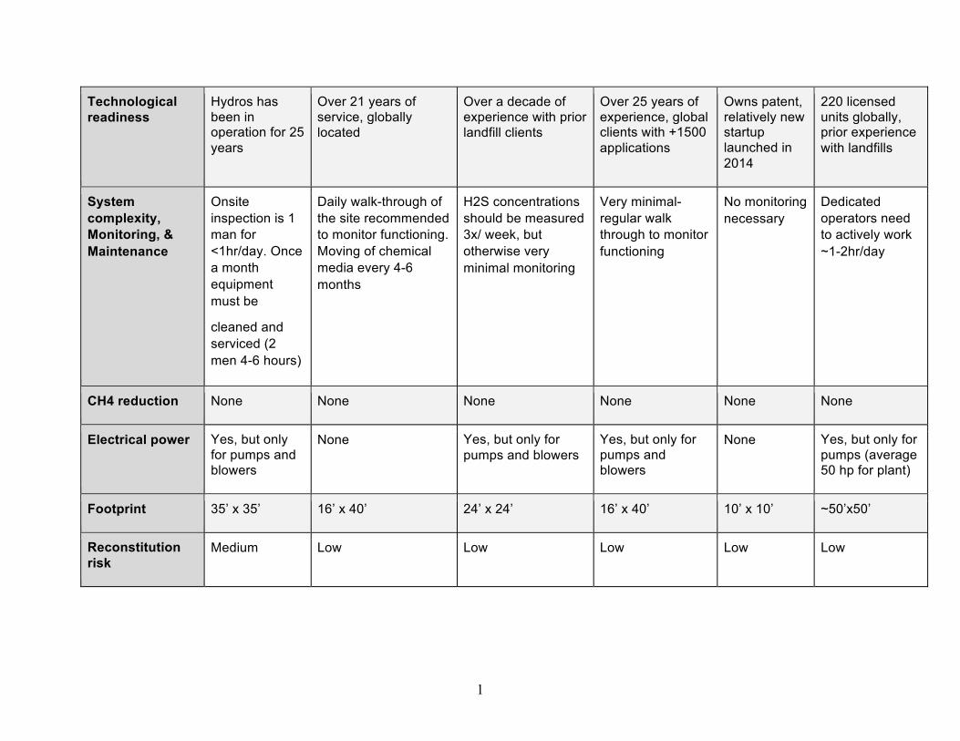
Table 5: Detailed Characteristics of Selected Technologies

Questions

Technologies

Hydros BioREM (non-biological process)

MV Technologies SulfaTreat SulfaChar LoCat

Technology type Liquid based oxidation process

Dry based, Iron Sponge

Dry based, Iron Sponge

Dry based, Iron Sponge

Dry based, activated carbon

Liquid based, oxidation process

Efficiency: Maximum tolerable H2S

20,000 ppmv 2000 ppmv 11,000 ppm H2S, 3000 lb/day of H2S

2000 lbs/day 100% H2S

100% H2S

Effectiveness: Reduction in H2S

<300 ppm >99% H2S removal <100-200 ppm 1 ppm <50-100 ppm

Up to 99.9+%. <50 ppmv

LFG & H2S Variability

None None Operating problems for bacterial suppl.

None None None

Water & wastewater

2000-3000 gallons of water needed daily. Sewer line is needed

None None Water injection recommended but not required

None Yes, .25 gpm/day. No sewage (water gets vented)

1

Technological readiness

Hydros has been in operation for 25 years

Over 21 years of service, globally located

Over a decade of experience with prior landfill clients

Over 25 years of experience, global clients with +1500 applications

Owns patent, relatively new startup launched in 2014

220 licensed units globally, prior experience with landfills

System complexity, Monitoring, & Maintenance

Onsite inspection is 1 man for <1hr/day. Once a month equipment must be

cleaned and serviced (2 men 4-6 hours)

Daily walk-through of the site recommended to monitor functioning. Moving of chemical media every 4-6 months

H2S concentrations should be measured 3x/ week, but otherwise very minimal monitoring

Very minimal- regular walk through to monitor functioning

No monitoring necessary

Dedicated operators need to actively work ~1-2hr/day

CH4 reduction None None None None None None

Electrical power Yes, but only for pumps and blowers

None Yes, but only for pumps and blowers

Yes, but only for pumps and blowers

None Yes, but only for pumps (average 50 hp for plant)

Footprint 35’ x 35’ 16’ x 40’ 24’ x 24’ 16’ x 40’ 10’ x 10’ ~50’x50’

Reconstitution risk

Medium Low Low Low Low Low