hydroelasticbehaviourofa structureexposedtoan...

rsta.royalsocietypublishing.org

ResearchCite this article: Colicchio G, Greco M,Brocchini M, Faltinsen OM. 2015 Hydroelasticbehaviour of a structure exposed to anunderwater explosion. Phil. Trans. R. Soc. A373: 20140103.http://dx.doi.org/10.1098/rsta.2014.0103

One contribution of 12 to a Theme Issue‘Advances in fluid mechanics for offshoreengineering: a modelling perspective’.

Subject Areas:mechanical engineering, ocean engineering,mathematical modelling, computationalmechanics, computer modelling andsimulation

Keywords:underwater explosion, compressibletwo-phase flow, hydroelastic fluid–structurecoupling, domain decomposition

Author for correspondence:G. Colicchioe-mail: [email protected]

Electronic supplementary material is availableat http://dx.doi.org/10.1098/rsta.2014.0103 orvia http://rsta.royalsocietypublishing.org.

Hydroelastic behaviour of astructure exposed to anunderwater explosionG. Colicchio1,2, M. Greco1,2, M. Brocchini3

and O. M. Faltinsen1,2

1CNR-INSEAN, The Italian Ship Model Basin, via di Vallerano 139,00128 Roma, Italy2Centre for Autonomous Marine Operations and Systems (AMOS),Department of Marine Technology, NTNU, Trondheim, Norway3Dipartimento di Ingegneria Civile, Edile e di Architettura,Università Politecnica delle Marche, Ancona, Italy

The hydroelastic interaction between an underwaterexplosion and an elastic plate is investigated num-erically through a domain-decomposition strategy.The three-dimensional features of the problem requirea large computational effort, which is reduced througha weak coupling between a one-dimensional radialblast solver, which resolves the blast evolutionfar from the boundaries, and a three-dimensionalcompressible flow solver used where the interactionsbetween the compression wave and the boundariestake place and the flow becomes three-dimensional.The three-dimensional flow solver at the boundariesis directly coupled with a modal structural solverthat models the response of the solid boundarieslike elastic plates. This enables one to simulate thefluid–structure interaction as a strong coupling, inorder to capture hydroelastic effects. The method hasbeen applied to the experimental case of Hung et al.(2005 Int. J. Impact Eng. 31, 151–168 (doi:10.1016/j.ijimpeng.2003.10.039)) with explosion and structuresufficiently far from other boundaries and successfullyvalidated in terms of the evolution of the accelerationinduced on the plate. It was also used to investigatethe interaction of an underwater explosion with thebottom of a close-by ship modelled as an orthotropicplate. In the application, the acoustic phase of thefluid–structure interaction is examined, highlightingthe need of the fluid–structure coupling to capturecorrectly the possible inception of cavitation.

2014 The Author(s) Published by the Royal Society. All rights reserved.

on May 29, 2018http://rsta.royalsocietypublishing.org/Downloaded from

http://crossmark.crossref.org/dialog/?doi=10.1098/rsta.2014.0103&domain=pdf&date_stamp=2014-12-15

mailto:[email protected]

http://dx.doi.org/doi:10.1016/j.ijimpeng.2003.10.039


http://rsta.royalsocietypublishing.org/

2

rsta.royalsocietypublishing.orgPhil.Trans.R.Soc.A373:20140103

.........................................................

1. IntroductionExplosions in fluids represent an important topic in many research fields. In medicine, forexample, implosions of micro-bubbles can be caused by the ultrasound used to remove kidneystones. For marine applications, two relevant dangerous examples are underwater explosions,which can damage close-by vehicles, and cavitating bubbles on propeller blades possibly leadingto erosion. Either when we are talking of micro- or macro-explosions, the common features are:(i) generation of an air bubble, (ii) propagation of a compression wave from the surface of thebubble, and (iii) eventual interaction of the compression wave with the surrounding structures.

Here, this phenomenon is investigated in the framework of underwater explosions, whichrepresents one of the most important causes of loss of navy vessels and it is a danger for close-bysubmarines, surface ships and offshore structures. This work continues the research proposed in[1]. There, a numerical solution strategy is proposed and described in detail. It is based on a one-dimensional–three-dimensional fluid-dynamic domain-decomposition (DD) coupling. A radialsolver is used to study the initial stages of the phenomenon, before the acoustic waves reacha structure, then, locally, a three-dimensional method handles the fluid–structure interaction.The three-dimensional sub-domain is limited by the body boundaries and the one-dimensional–three-dimensional interface across which information is transmitted. In [1], the structure wasmodelled as rigid and preliminary studies of the fluid–structure interactions accounting for elasticstructural behaviour and an approximated coupling with the fluid were performed using onlythe radial solver over the whole fluid domain and for the whole evolution. On the contrary, in thepresent contribution the fluid-dynamic problem is described with the same hybrid method but thefluid–elastic structure coupling is fully simulated. This enables one to investigate the hydroelasticbehaviour, which destroys any radial symmetry in the flow. Some preliminary results have beendocumented in [2]. The paper is structured as follows. The proposed method is illustrated in §2,with emphasis on the new aspects. Two selected important cases are analysed in §3. Finally, someconclusions and lines for future research are proposed in §4.

2. The numerical solverUnderwater explosions are characterized by several complex phenomena: (i) multi-phase flow,involving at least water and gas cavities resulting from the blast, (ii) flow compression, involvingthe propagation of acoustic waves during cavity expansion, and (iii) transition from compressibleto incompressible flow dynamics during the later cavity oscillations.

The developed solution strategy focuses on underwater explosions and their interaction withstructures far from other boundaries, such as the sea floor or the sea surface. The methodintroduced in [1,3] combines two solvers within a zonal approach to capture the complex anddetailed flow features described above. Here, the main aspects of the solver are described,while more details can be found in [1], where, also accuracy and convergence properties of thetwo involved fluid-dynamic solvers and the structural modelling are assessed. Moreover, thescalability of the parallelized part of the method, i.e. the relationship between required CPU timeand number of processors, is provided. Thus, these aspects are not discussed here.

(a) The compressible solver for two-phase flows: three-dimensional and radial solutionsWe examine the flow caused by an underwater explosion assuming that the chemical reactionsand the detonation phase have ended and have generated a gas cavity with known initial physicalproperties. This flow involves at least two phases, gas and water, and it is, in general, three-dimensional and compressible. We neglect viscous effects and solve the problem in a CartesianEarth-fixed coordinate system (x, y, z). We retain flow nonlinearities since nonlinear features arein general important to properly capture the initiation and propagation of the acoustic waveswhich, at the first stages, are always rather strong and that can still be important also duringa wave–body interaction if the explosion occurs sufficiently close to the wall and/or if the



3


.........................................................

explosion is sufficiently strong. Moreover, nonlinear flow features could be induced by stronghydrodynamic–structural coupling. Under these assumptions, the governing equation can beformally written as

∂U∂t

+ ∇ · F = 0. (2.1)

Here, V = (u, v, w) is the velocity, p the pressure, ρ the density, E = ρ[e + (u2 + v2 + w2)/2] thetotal energy, U = [u, ρu, ρv, ρw, E]T the vector of fluid variables and F = [Fx, Fy, Fz]T the vectorof fluxes with Fx = [ρu, ρu2 + p, ρuv, ρuw, (E + p)u]T, Fy = [ρv, ρuv, ρv2 + p, ρvw, (E + p)v]T andFz = [ρw, ρuw, ρvw, ρw2 + p, (E + p)w]T. To complete the problem, an equation of state (EOS) ofthe form

ρe = ff(ρ)p + gf(ρ) (2.2)

is assumed for the specific internal energy e. The functions ff and gf depend on the fluid properties,as indicated by the subscript f. In particular, for the gas generated by the explosion, they are setin agreement with the Jones–Wilkins–Lee EOS [4] and for the water they follow an isentropicTait relation [5]. Equations (2.1) and (2.2) must be complemented by the initial and boundaryconditions which apply in the examined case.

Within the three-dimensional framework, equation (2.1) is solved numerically with a second-order finite-difference scheme in space and integrated in time with a total variation diminishingthird-order Runge–Kutta scheme (see [6]), with the fluxes in each fluid modelled with a Harten–Lax–van Leer contact Riemann solver (see [7]).

A two-shock approximation to the Riemann problem is enforced at the gas–cavity interfaceas proposed in [8] solving for the two nonlinear characteristics intersecting at the interfaceand using mass and momentum jump conditions for the transmitted and reflected shocks. Theresulting equation system is nonlinear and it is solved iteratively with a Newton–Raphsonmethod providing values of (V · n)i = ui, pi, ρL

i and ρRi , respectively, the normal velocity and

pressure at the interface and the left and right density. Here, ‘left’ means ‘inside the gas cavity’ and‘right’ means ‘in water’. The estimated values for ρL

i and ρRi are corrected by enforcing an isobaric

condition across the interface so to avoid numerical errors in the pressure. This interface algorithmis based on a ghost fluid method (see [8]) and provides the conditions across the interface to eachfluid. Once all interface variables are known, the fluxes F can be calculated in each fluid and theproblem can be stepped forward in time. To follow the evolution of the gas–water interface, theuse of the three-dimensional Eulerian solver requires an additional technique. In the present case,a colour-function method is adopted, advecting in time the signed distance (positive in one fluidand negative in the other) from the interface. This is known as level-set function φ and its zerovalue identifies the interface, which can be reconstructed in time by interpolating the φ values atthe centre of the cells. φ is advected in time using the equation

∂φ

∂t+ V i · ∇φ = 0, (2.3)

where V i is the interface velocity calculated like in [8]; in particular the normal velocity comesfrom the interface solution strategy described above, while the two tangential components areobtained as averages between the solutions in the two fluids. Once the instantaneous interfaceposition is identified as φ = 0, the Riemann problem described above is solved across theinterface to ensure proper reflection and transmission of shock waves.

To make the solution efficient in time, an adaptive mesh refinement is used according to [9].The grid is subdivided in blocks and each block can be dynamically (i.e. during the simulation)split into eight smaller blocks in case a finer mesh is locally required, or neighbouring blocks canbe merged into one single, larger block when the flow variations become sufficiently small. Thissplitting/merging process is controlled by a criterion which monitors the intensity of the fluidvariable ∇p. Within such an adaptive algorithm, an interpolation strategy can be required; here,a second-order polynomial expression is chosen consistently with the order of accuracy of thethree-dimensional numerical scheme.



4


.........................................................

The described solver can incorporate the presence of solid and deformable boundaries like,respectively, the sea floor and the sea surface. For both of them, a level-set technique can beapplied when the grid is not adapted to the boundary, as may occur for the evolving air–waterinterface. One must, however, note that special care must be taken when the acoustic waveresulting from an explosion reaches the sea surface, because the interaction involves, amongothers, partial reflection and cavitation phenomena (e.g. [10]).

Within the radial solver, the governing equation (2.1) of the problem reduces to a one-dimensional Euler equation in the radial direction, r, of the form

∂U∂t

+ ∂F∂r

= S, (2.4)

with U = [ρ, ρu, E]T, F = [ρu, ρu2 + p, (E + p)u]T and S = 2[ρu/r, ρu2/r, u(E + p)/r]T. Here, u is theradial velocity, p the pressure, ρ the density and E the total energy ρ(e + u2/2). The same EOSs ofthe three-dimensional case are used for the specific internal energy e to close the problem for gasand water. The numerical implementation of the one-dimensional formulation is based on a first-order, finite-difference scheme in space and time, which proved to be also very accurate whencompared with other numerical solutions, for fully one-dimensional problems and problemswith radial symmetry, even for long-time evolutions [1]. For this reason, no attempt was madeto implement a second-order formulation to improve the solution efficiency. The fluxes and theinterface conditions are handled as in three dimensions.

For both three-dimensional and radial formulations of the solver, the time step is dynamicallychosen on the basis of a Courant–Friedrichs–Lewy stability condition, which in our case reads�t ≤ k · CFL. CFL is min(�r/max(|u − c|, |u + c|)) for the one-dimensional solution and it issimilarly defined for the three-dimensional solution. The safety factor k is chosen to avoiddiverging behaviours of the solution. Here, �r is the local spatial discretization, and c the localspeed of sound, so min() and max(), respectively, mean minimum and maximum values in thecomputational domain.

If the explosion occurs very far from the solid boundaries, a spherical gas cavity is formed,whose evolution is well approximated by a radial symmetry, as gravity does not play a relevantrole and the hydrostatic pressure enters the problem only in terms of the surrounding backgroundpressure for the bubble. This has motivated the implementation of a ‘one-dimensional’ radialsolution. When the explosion interacts with a structure, the one-dimensional solver can be stillcombined with a structural model, as long as hydroelastic effects are negligible. This allows asimplified study of the fluid–structure interactions. In particular, this means that a radial solvercan be applied until the acoustic wave reflected from the structure reaches the blast bubble andgoes back to the body. This alternative has been implemented and assessed in [1] and is alsoanalysed in the physical investigation documented in §3.

Here, a three-solvers coupling is used. The one-dimensional method can be applied at any timein a sub-domain sufficiently far from the region where three-dimensional effects caused by thefluid–body interaction are important, while the three-dimensional method is used to model thenear-body flow. In this way, a composite solver, able to describe the whole stages of the fluid–bodyinteraction, can be built and, at the same time, the computational costs (CPU time) are limited asmuch as possible.

(b) One-way time–space domain decomposition for compressible two-phase flowsThe two compressible solvers described in §2a can be combined within a DD strategy toinvestigate underwater explosions with initial radial symmetry. Here, this hybrid method isproposed as a one-way, time–space coupling, which means that the radial solver is thought to beused over the whole domain for time t ≤ t∗, where t∗ represents the time at which the compressionwave approaches the one-dimensional–three-dimensional boundary. At t = t∗, the DD is switchedon and the three-dimensional solver is introduced in a zone containing the structure where three-dimensional effects are expected to be important, with initial conditions provided by the radial



5


.........................................................

solver. The latter is still used in the rest of the fluid domain and provides also the boundaryconditions for the three-dimensional solver at the common interface. The position of the one-dimensional–three-dimensional boundary can be stated at the beginning of the simulation or itcan be changed to reduce as much as possible the three-dimensional domain.

The one-dimensional–three-dimensional solver–solver interface is not meant to be a sharpsurface but it is conceived as an overlapping region between the spherical sub-domain of theradial solution and the prismatic sub-domain of the three-dimensional solution. Within thisoverlapping layer, the fluid variables are forced to smoothly vary from the values provided byone solver to those estimated by the other. The use of an overlapping region has been found togive a more robust numerical solution than the use of a sharp interface. On the other hand, insidethe overlapping region both solvers are applied, so the thickness of this layer must be as smallas possible. Here, this thickness is set 4�xloc, �xloc being the local size of the three-dimensionalcomputational grid, and a cosine function is used for the smooth variation of the solution acrossthe overlapping region itself. The DD strategy significantly limits the computational costs withrespect to using a compressible three-dimensional solver over the whole domain and for the entiretime evolution. This can be easily understood if one considers that the computational cost andmemory space for the three-dimensional solver increase with N3, N being the number of pointsper spatial direction; they increase instead with N for a radial solution.

If the explosion occurs sufficiently close to boundaries, such as the sea surface, the sea floor,a marine structure, so that no radial symmetry can be assumed even near the bubble, then theabove-proposed DD strategy cannot be applied and the fully three-dimensional solver must beused from the beginning of the simulation and everywhere in the fluid domain.

(c) Structural modellingA marine structure exposed to a blast can experience elastic and plastic deformations even leadingto rupture. The initial phase, i.e. the acoustic phase, of the incident flow is important for the localforcing on the structure and is analysed by this study. The aim is to investigate the importanceof hydroelastic effects and other involved phenomena. This is done assuming only elasticdeformations of the body can take place. It means the use of a simplified structural modelling,which has, nevertheless, proved to be able to capture the inception for plastic deformations, aswell as the maximum strain rate and dynamic yield stress at hand [1]. Assuming the structure tobe the bottom of a vessel, it is modelled as a rectangular orthotropic plate with length L and widthB in the x and y directions, respectively. The plate is assumed to undergo a linear deformationw(x, y, t) governed in time and space by the equation

m∂2w∂t2 + Dx

∂4w∂x4 + 2BB

∂4w∂x2∂y2 + Dy

∂4w∂y4 = p(x, y, w, t). (2.5)

Here, m is the average plate mass per unit area, Dx and Dy are its flexural rigidities inthe two main directions and BB is its effective torsional rigidity (e.g. [11]). On the right-handside, p is the local hydrodynamic pressure acting on the plate which depends on space, timeand w, in particular on its time derivatives. This equation is solved with a modal approach byusing separation of variables and expressing the deformation w as bi-linear combinations ofthe eigenfunctions of vibrating beams satisfying the plate boundary conditions in both x andy directions. Each of these combinations represents a plate mode and it is associated with anunknown amplitude depending on time. The number of eigenfunctions in x and y is taken tobe finite, say Nx and Ny, leading to N = Nx · Ny plate modes, then the modal expression of wis introduced in equation (2.5) and the resulting equation is projected along each of the N platemodes. This leads to a linear ordinary differential (in time) equation system for the N unknownamplitudes of the modes.

For simplicity purposes, we have here used a ‘thin-plate’ theory (e.g. Kirchhoff–Love platetheory). However, nothing prevents the use of a more complicated model valid for thick plates(e.g. Mindlin–Reissner plate theory). In fact, the DD strategy is independent of the chosen plate



6


.........................................................

theory. Hence, the mentioned strategy can be applied also in combination with higher orderplate theories, as long as the plate model gives both the displacement and the displacementvelocity back to the fluid solver and receives as input from it the fluid pressure on the plate.When the DD strategy is used, and the three-dimensional solver is used in the fluid regioncontaining the structure, p is obtained by solving the fluid–structure coupled problem, i.e. it isaffected by the plate elastic behaviour. In more detail, the structure represents a solid deformableinterface immersed in the fluid domain. This interface is identified at any instant by a level-setfunction, similarly to what is done for the gas–water interface. Inside the body, ‘guard’ cells[9] are introduced which can be considered as a sort of ‘ghost cells’. In those cells, the velocitycomponent vN(P) normal to the body surface at point P is made equal to −vN(Pmirror) + 2vN wall,where vN wall is the normal velocity of the wall and Pmirror is the mirror point of P inside the fluid.For the tangential components, it is vτ (P) = vτ (Pmirror). Then, the fluid-dynamic problem (2.1) canbe prolonged in time and provides the pressure. The latter can be extrapolated on the structure,i.e. along the iso-surface with zero value of the level-set function associated with the body andused in the structural problem (2.5) to find w. Once this is known, the position of the body canbe updated in time through use of the level-set technique so that the new body–fluid boundarycondition can be enforced again in the fluid dynamic problem. As we assume elastic and smalldeformations, the errors are very limited if the body-boundary condition is applied on the meanplate configuration.

If the radial solution is used for simulating the incident acoustic wave, the direct full fluid–structure interaction cannot be examined. The coupling is, then, approximated assuming that thelinear superposition principle is valid for the fluid–body interaction. Therefore, the pressure p isdecomposed as

p(x, y, w, t) = 2pin(r, t) − ρccos(θ )

∂w∂t

+ added-mass contribution, (2.6)

where ρ and c are the density and speed of sound in calm water, pin is the incident wave pressureand θ is the angle between the direction of the incident wave reaching locally the plate and theplate normal vector. The first two terms on the right-hand side of equation (2.6) are importantduring the acoustic phase and represent the sum of the incident and reflected (from the wall)wave pressure. This leads to twice pin for a fixed wall ‘plus’ an acoustic wave-radiation dampingin the case of rigidly moving or deformable plate, consistent with the theory developed in [12] forexplosion waves interacting with plates. The last term represents an incompressible added-masscontribution, which is important when the water behaves as an incompressible fluid and if theplate oscillates as a consequence of the interaction with the incident acoustic wave. In the presentimplementation, the acoustic wave-radiation damping term is switched off when pin becomeshalf of the acoustic pressure associated with the incident wave and, then, the added-mass term isswitched on.

The added-mass contribution for each plate mode is estimated in an approximate way,studying the radiation problem for each plate mode and assuming that the plate is surroundedby a fixed wall and then by a flat ‘free surface’ with velocity potential ϕ = 0. This means that it is ahigh-frequency added mass estimate and introduces, in general, some inaccuracies. For example,for a ship the structure of interest could be the bottom of the vessel, eventually exposed to anexplosion. In this case, the plate would be used to model the grillage on the bottom and thismeans that it cannot be at the same level of the free surface. The surrounding ‘free surface’ usedin the added mass solution is meant to avoid a purely Neumann-type problem, which would leadto a solution in general dependent on an arbitrary constant. The dimensions of the fixed wall areassumed to be large enough that by increasing them there is no significant influence on the addedmass. The problem has been solved numerically with a zero-order boundary element method bydiscretizing the plate, the fixed wall and the flat ‘free surface’ with quadrilateral panels and usingan indirect source formulation as in [13]. The added-mass calculations have been successfullyassessed against reference solutions for the case of added mass in heave of a rigid plate and for acase of added mass for the elastic modes of a simply-supported uniform plate [1].



7


.........................................................

0.6

0.4

0.2

0.2345 m

steel plate: 2.54 m thick

aluminium plate: 0.01 m thick

1 m

1 m

: ri,max =~ 0.16 m

: ri =~ 0.06 m at t = 0.7 ms

: ri = radius of gas–water interface

t (ms)

r (m)

plate

3D sub-domain

1D sub-domain

0 10 20 30

r = rp = 0.7 m

charge

(b)(a)

Figure 1. Underwater-explosion experiments of Hung et al. [14]. (a) Experimental set-up. (b) Evolution of the gas cavity asobtained by the radial solution and radial extension of the one-dimensional and three-dimensional solvers in the DD strategyused for this test case. (Online version in colour.)

3. Physical investigationsHere, two cases of underwater explosions are examined, with specific focus on the evolution andcharacteristics of hydroelastic fluid–structure coupling.

(a) Underwater explosion: interaction with a uniform plateThe examined case refers to the underwater-explosion experiment of Hung et al. [14] and thestudy is performed using both (i) the radial fluid-dynamic solution and approximate couplingwith the structure and (ii) applying the DD strategy and the full fluid–structure coupling. In thetests, a mixture of DP60 detonator and Datasheet causes an underwater explosion interactingwith an air-backed aluminium plate mounted on a steel frame (figure 1a). Different standoffdistances rp of the charge centre from the plate were studied but the time histories of the incident-wave pressure and induced plate acceleration are only available for the distance of 0.7 m. Hence,the latter is examined here. To reproduce correctly the incident-wave pressure, the parametersfor the EOS (2.2) and, in particular, the initial radius, pressure and density of the gas cavityresulting from the explosion should be identified. The challenge is the unconventionality of theexplosive; therefore the following identification strategy for the equivalent TNT parameters wasimplemented. In [14], Hung and co-authors assumed a radial symmetry of the explosion becauseof the large distance of its centre from the tank boundaries and expressed the incident-wavepressure at a given radial distance as follows:

p(t, r, W) = pmax(W, r) e−t/θ(W,r). (3.1)

Here, W is the charge weight and r the standoff distance of the chosen fluid location from thecore of the explosion. Moreover, empirical formulae were proposed for the maximum pressurepmax and the pressure rate of decay θ as functions of W and r.

In our model, we take as valid the EOS (2.2) both for water and gas, but, as we do notknow the values of the involved coefficients for the used explosive mixture, as well as allrequired initial conditions, we model the explosion as due to an equivalent TNT charge, forwhich the coefficients of the related EOS are known. The equivalent explosion is identifiedenforcing that pmax obtained by using the TNT charge at a given distance r is the same asthat provided by equation (3.1). In particular, r = 0.0895 m was chosen as the target location



8


.........................................................

50

25

0

24

10

4

0 0

12

0

p–

p 0 (M

Pa)

t (ms) t (ms) t (ms) t (ms)0.1 0.08 0.16 0.21 0.28 0.42 0.49

Figure 2. Underwater-explosion experiments of Hung et al. [14]: in each plot, time history of the empirical (dashed line) andradial numerical (solid line) incident-wave pressure at a fixed radial distance r. From left to right: r = 0.0895, 0.1590, 0.3593and 0.7 m. p0 is the ambient pressure. (Online version in colour.)

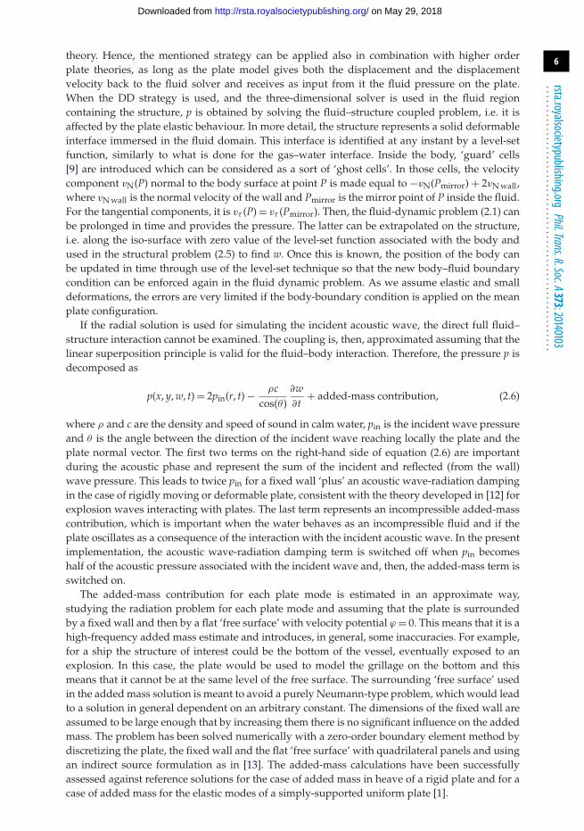
because it is relatively close to the explosion source and, further, is the smallest distance forwhich tabulated values for pmax and θ are provided in [14]. This resulted in a cavity with initialradius r0 = 0.03 m, density ρ0g = 1630.0 kg m−3 and pressure p0g = 2 × 1010 Pa. Figure 2 shows thecomparison between the incident-wave pressure as predicted by the radial numerical solutionand by the empirical formula (3.1) at four radial distances from the initial explosion. The resultsreveal a good description of the pressure decay in time. With reference to the maximum pressure,as expected, the two predictions are identical at r = 0.0895 m while the present solution tends tounderestimate more and more the empirical pmax for increasing distances from the charge. Thisdoes not mean that the numerical solution necessarily provides a less accurate pressure predictionmoving far from the initial explosion. In fact, the good comparison with the incident-wavepressure observed at r = 0.7 m, which corresponds to the radial distance of the plate, highlightsthe good performances of the model. In more detail, figure 3 reveals that, once the rising timesof the two solutions are synchronized (this involving a shift of 0.018 ms), the time history of thenumerical pressure reproduces very well the experimental one of Hung et al. [14]. This means thatthe numerical explosion has a small error in terms of propagation speed, i.e. it is slightly fasterthan the physical one, but it can capture better the maximum experimental pressure than theempirical formula proposed in [14] and behaves similarly to such a formula in terms of time decay.Moreover, despite the simplifications used in modelling the explosion, the numerical predictionof 30.5 ms for the first oscillation period of the gas cavity (figure 1b) is not far from the value of26.7 ms observed in the model tests.

The interaction between the underwater explosion and the target plate was studied using, forthe fluid dynamic problem, both the full radial solution and the DD strategy. In the latter case,the radial solver extended from the position of the initial explosion up to a radial distance of0.42 m and the three-dimensional sub-domain overlapped with it within a layer of about fourlocal cells and, thus, included the plate with the steel casing. This means that the gas cavity wasalways inside the radial sub-domain during the examined evolution (figure 1b), therefore the one-dimensional solver simulated a two-phase flow while the three-dimensional method examineda one-phase flow interacting with the structure. In the case of the full radial solution, only thealuminium plate is modelled as a uniform elastic plate; in the DD case, also the steel casing ismodelled, but, for numerical convenience (i.e. to make the thickness to be a multiple of the blocksize), it is assumed slightly thicker than it is in reality, with a thickness of 0.35 m. Since duringthe examined evolution, the pressure wave does not reach the back side of the real steel casing, theerror connected with using a thicker structure is expected to be negligible. In addition, to limitthe CPU-time requirements, the symmetry of the problem is accounted for and only one-fourth



9


.........................................................

4

2

0.45 0.46 0.47t (ms)

0.48

plate

charge

incidentpressuresensor

measured

r = 0.7 m

r = 0.7 m

numerical solution(shifted back of 0.018 ms)

p–

p 0 (M

Pa)

Figure 3. Underwater-explosion experiments of Hung et al. [14]: experimental and radial numerical incident-wave pressure atr = 0.7 m. (Online version in colour.)

of the fluid domain is simulated in the three-dimensional sub-domain. In both cases, i.e. usingthe one-dimensional or the DD fluid-dynamic solver, the simulations were carried out assumingeither a restrained or a simply-supported plate with Nx = Ny = 10 beam modes, leading to N = 100plate modes.

In the experiments, the acceleration at the centre of the plate was measured during the initialstage of the wave–body interaction. This is examined in figure 4, which shows a much bettercomparison of both the radial solution with approximated fluid–structure coupling and the DDsolution with full fluid–structure coupling with the experimental acceleration than that givenby a recent numerical simulation documented in [15], which employs an analytical techniquefor the fluid-dynamic problem and an elastic dynamic response of the structure. In particular,both the solvers here proposed: (i) consistently reproduce the rising phase of the measuredacceleration and (ii) indicate the inception of oscillations which characterize the experimentaldata. In addition, the measurements indicate a high-frequency behaviour, which cannot beexplained on the basis of the information available from the work in [14]. The one-dimensionaland three-dimensional solutions show a similar behaviour during the first stages of the evolution,involving a fast rise of the acceleration up to a maximum value which is followed by a decay.This suggests that at the beginning of the interaction, the radial symmetry is still valid and thecoupling between fluid and structure is weak. Data of maximum acceleration at the centre of theplate are summarized in table 1 together with the maximum velocity at the centre of the plate,both referring to the initial phase of the incident-wave pressure interaction with the structure.As in the experiments only the acceleration was measured, and the maximum velocity has beenestimated by integrating in time the measured acceleration. In this context, the high-frequencybehaviour of the recorded acceleration represents a source of error both for the maximumacceleration and for the maximum velocity. An inspection of the results reveals that both one-dimensional and DD maximum accelerations agree better with the measurements in [14] than thefinite element method (FEM) predictions reported in the same paper. The DD results are slightlyworse than the one-dimensional predictions. However, such a slightly poorer performance canbe explained in view of: (i) the high-frequency oscillatory behaviour in the measurements, (ii) thesensitivity during this first stage of the fluid–body interactions to the physical conditions, and(iii) the numerical choices. The same arguments hold also for the maximum velocity, which isoverpredicted by the DD solution. In this case, an additional source of error is related with thetime-integration procedure possibly used for the measured accelerations.



10


.........................................................

3.5

3.0

2.5

2.0

1.5

1.0

0.5

–0.5

–1.0

–1.50.45 0.50 0.55 0.60

t (ms)0.65 0.70

0

DD simply-supported plateDD restrained plate1D simply-supported plate1D restrained platenumerical by Wang et al. [15]measured by Hung et al. [14]

acce

lera

tion

(G×

104 )

1 2 3 4

Figure 4. Underwater-explosion experiments of Hung et al. [14]: evolution of the acceleration at the centre of the plate asmeasured in [14], predicted in [15] and by the present one-dimensional (1D) and DD solutions for both restrained and simply-supported plate. The four time instants labelled from 1 to 4 and indicated by the vertical dotted lines correspond, respectively,to the top-centre, top-right, bottom-left and bottom-right panels of the DD simulation given in figures 5 and 6. (Online versionin colour.)

Table 1. Maximum velocity and acceleration (given in terms of gravity acceleration G) induced at the centre of the plate.Experiments and FEM results are from [14]; 1D and DD refer to the present solutions obtained using, respectively, the radialand the DD strategy for the fluid-dynamic solver; RP, restrained plate; SSP, simply-supported plate.

experiments FEM 1D RP 1D SSP DD RP DD SSP

Vmax (m s−1) 2.63 2.46 2.48 2.57 3.70 3.57. . . . . . . . . . . . . . . . . . . . . . . . . . . . . . . . . . . . . . . . . . . . . . . . . . . . . . . . . . . . . . . . . . . . . . . . . . . . . . . . . . . . . . . . . . . . . . . . . . . . . . . . . . . . . . . . . . . . . . . . . . . . . . . . . . . . . . . . . . . . . . . . . . . . . . . . . . . . . . . . . . . . . . . . . . . . . . . . . . . . . . . . . . . . . . . . . . . . . . . . . .

amax (G × 104) 3.08 3.54 3.19 3.19 2.78 2.76. . . . . . . . . . . . . . . . . . . . . . . . . . . . . . . . . . . . . . . . . . . . . . . . . . . . . . . . . . . . . . . . . . . . . . . . . . . . . . . . . . . . . . . . . . . . . . . . . . . . . . . . . . . . . . . . . . . . . . . . . . . . . . . . . . . . . . . . . . . . . . . . . . . . . . . . . . . . . . . . . . . . . . . . . . . . . . . . . . . . . . . . . . . . . . . . . . . . . . . . . .

The time evolutions of the one-dimensional and DD accelerations start to diverge as the curvesapproach the first minimum and this leads to clear differences in the later oscillations (figure 4).At this stage, the two DD solutions, assuming either restrained or simply-supported plate, aremore consistent with the experiments, better capturing the second oscillation peak and indicatinga more complex fluid–structure interaction than that described by the one-dimensional solver.

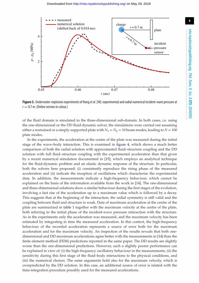
To better understand the features involved in such a coupling, the DD solution is examinedin further detail. The restrained-plate condition is focused upon, as representative of both plateedge conditions (restrained and simply-supported) which behave rather similarly. Figures 5and 6 illustrate the evolution of the pressure iso-surfaces with p = 73.6 × 104 Pa together with,respectively, the pressure and normal velocity on the plate.

As time goes by, the wave pressure interacts with the plate, leading to pressure and velocitywhich increase on the structure with radial symmetry (see top-left and top-centre panels offigures 5 and 6). At this stage, the acceleration at the plate centre is still limited, but quicklyincreases (see time labelled as ‘1’ in figure 4). The radial symmetry loosens in time due tothe finite dimensions of the plate (see top-right panels of figures 5 and 6). This corresponds,approximately, to the first minimum of the acceleration at the plate centre (see time labelledas ‘2’ in figure 4). When the pressure wave reaches the edges of the plate, the pressure andvelocity of the structure are characterized by important contributions from the higher modes (seebottom panels of figures 5 and 6) and this suggests the possible need of more modes in the plate



11


.........................................................

2.2 × 106

2.0 × 106

1.0 × 1061.2 × 1061.4 × 1061.6 × 1061.8 × 106

200 000400 000600 000800 000

2.2 × 106

2.0 × 106

1.0 × 1061.2 × 1061.4 × 1061.6 × 1061.8 × 106

200 000400 000600 000800 000

2.2 × 106

2.0 × 106

1.0 × 1061.2 × 1061.4 × 1061.6 × 1061.8 × 106

200 000400 000600 000800 000

2.2 × 106

2.0 × 106

1.0 × 1061.2 × 1061.4 × 1061.6 × 1061.8 × 106

200 000400 000600 000800 000

2.2 × 106

2.0 × 106

1.0 × 1061.2 × 1061.4 × 1061.6 × 1061.8 × 106

200 000400 000600 000800 000

2.2 × 106

2.0 × 106

1.0 × 1061.2 × 1061.4 × 1061.6 × 1061.8 × 106

200 000400 000600 000800 000

p (N m–2) p (N m–2) p (N m–2)

p (N m–2) p (N m–2) p (N m–2)

Figure 5. Underwater-explosion experiments of Hung et al. [14]: numerical DD evolution of the pressure iso-surfaces withp= 73.6 × 104 Pa together with the pressure on the plate. Here, p indicates p − p0, with p0 the ambient pressure. Timeincreases from left to right and from top to bottom and corresponds to: t = 0.32, 0.45, 0.48, 0.492, 0.510 and 0.514 ms. Thesimulation has been performed with minimum cell size of 0.00625 m and assuming N = 100 for the plate modes. The plate isrestrained. (Online version in colour.)

modelling, to properly describe the structural behaviour. An identical need can be found for thesimply-supported plate, as confirmed by the similar evolution of the acceleration in figure 4. Theneed for the increase of modes is confirmed by the solution of figure 7, obtained with N = 400plate modes and for two different discretizations. There the acceleration of the plate is comparedwith the experimental one. The initial behaviour of the acceleration is similarly represented bythe two simulations; the shorter duration of the initial peak obtained with the finer mesh is due tothe lower numerical dissipation undergone in this case. After t = 0.47 ms, higher modes play animportant role (see also figure 4) and cause a weaker deceleration of the plate. For higher modes,a finer mesh is necessary to capture the hydroelastic coupling.

At this stage, the acceleration at the plate centre reaches a second maximum, which is smallerthan the first peak due to the hydroelastic effects (see time labelled as ‘3’ in figure 4).

The reflected compression wave and the propagating one have different intensities because ofthe effect of the plate motion on the former. Moreover, the transmitted wave changes its curvature,in particular it tends to become cylindrical with axis around the edge of the plate. The combinationof these three ingredients causes the interaction between the reflected and transmitted wave todetermine the profile illustrated in the bottom–right panels of figures 5 and 6.

At this stage (see the bottom-right panel of figure 6), the plate velocity is very large near thecorners as a consequence of the pressure wave reflection from the wall. The last instant shownfor the DD prediction of the acceleration at the centre of the plate (see time labelled as ‘4’ infigure 4) corresponds to the last instant of the pressure iso-surfaces evolution discussed here.This corresponds to the time when the pressure wave reflected from the structure has almostreached the interface between the one-dimensional and three-dimensional sub-domains, so thesimulation has been stopped. To prolong the solution in time, a dynamic enlargement of the three-dimensional sub-domain at the expenses of the one-dimensional sub-domain should be used, asdiscussed in §2.



12


.........................................................

1.0

0.9

0.8

0.7

0.6

0.5

0.4

0.3

0.2

0.1

–0.1

–0.2

–0.3

–0.4

–0.5

–0.6

1.0

0.9

0.8

0.7

0.6

0.5

0.4

0.3

0.2

0.1

–0.1

–0.2

–0.3

–0.4

–0.5

–0.6

1.0

0.9

0.8

0.7

0.6

0.5

0.4

0.3

0.2

0.1

–0.1

–0.2

–0.3

–0.4

–0.5

–0.6

1.0

0.9

0.8

0.7

0.6

0.5

0.4

0.3

0.2

0.1

–0.1

–0.2

–0.3

–0.4

–0.5

–0.6

1.0

0.9

0.8

0.7

0.6

0.5

0.4

0.3

0.2

0.1

–0.1

–0.2

–0.3

–0.4

–0.5

–0.6

1.0

0.9

0.8

0.7

0.6

0.5

0.4

0.3

0.2

0.1

–0.1

–0.2

–0.3

–0.4

–0.5

–0.6

dy/d

t(m

s–1)

dy/d

t(m

s–1)

dy/d

t(m

s–1)

dy/d

t(m

s–1)

dy/d

t(m

s–1)

dy/d

t(m

s–1)

Figure6.Underwater-explosion

experim

entsofHungetal.[14]:num

ericalDDevolution

ofthepressureiso-surfaceswithp=

73.6

×104Patogetherwiththenormalvelocity(dy/dt

=v)ontheplate.Other

arrangementsasincaption

offigure5.(O

nline

versionincolour.)



13


.........................................................

3.53.02.52.01.51.00.5

–0.5–1.0–1.5

0

DD Dxmin = 6.25 × 10–3 N = 400DD Dxmin = 4.00 × 10–3 N = 400

experiment

acce

lera

tion

(×10

4 G)

t (ms)0.45 0.50 0.55 0.60 0.65 0.70

Wang et al. [15]

Figure 7. Underwater-explosion experiments of Hung et al. [14]: numerical DD evolution acceleration at the centre of the simplysupported plate, for two different discretizations and N= 400. (Online version in colour.)

a

N.hwyA.

t

twy

tfy

bfy

Zoy

b

N.hwxA.

t

twx

tfx

bfx

Zox

B

Llongitudinals

transverse frames

bb

bb

bb

bb

bb

a

a

a

a

arrangement from full-scale experiments by Smith [16]

Figure 8. Steel-grillage arrangement for the bottom of navy ships as studied experimentally in [16]. Here, L and B arethe longitudinal and transversal length of the grillage, respectively, a and b are the distances between two transverseframes and two longitudinal stiffeners, respectively. Grillage 1a of [16] with four transverse frames and four longitudinalstiffeners is here examined. The parameters are L= 6.096 m, B= 3.048 m, t = 0.008 m, hwx = 0.15367 m, twx = 0.00721 m,bfx = 0.07899 m, tfx = 0.01422 m, hwy = 0.25756 m, twy = 0.00937 m, bfy = 0.12548 m and tfy = 0.01829 m.

Table 2. Equivalent orthotropic plate for the steel-grillage arrangement 1a of [16] documented in figure 8. The values are givenin SI units. L and B are the plate extensions in x- and y-direction, respectively.σy is the yield stress of the plate.

L B m Dx Dy BB σy

6.069 3.048 85.785 1.262 × 107 3.517 × 107 2.614 × 104 250.4 × 106. . . . . . . . . . . . . . . . . . . . . . . . . . . . . . . . . . . . . . . . . . . . . . . . . . . . . . . . . . . . . . . . . . . . . . . . . . . . . . . . . . . . . . . . . . . . . . . . . . . . . . . . . . . . . . . . . . . . . . . . . . . . . . . . . . . . . . . . . . . . . . . . . . . . . . . . . . . . . . . . . . . . . . . . . . . . . . . . . . . . . . . . . . . . . . . . . . . . . . . . . .

(b) Underwater explosion: interaction with a navy-ship bottomHere, the possible consequences of an underwater explosion on the bottom of a navy ship areexamined using the DD decomposition and the full fluid–structure coupling.

The bottom grillage arrangement is chosen to be that of configuration 1a among those studiedexperimentally in [16] (see the sketch of figure 8) and an equivalent orthotropic plate has beenidentified with main parameters given in table 2 and taken to be restrained at all edges.

The modelled plate has been forced by the underwater explosion caused by a TNT chargedocumented in [17], which is used as a representative sample of typical explosions, to assesspossible ship damages. For this explosion, all parameters needed for the gas and liquid EOSs



14


.........................................................

14

4 m

1D

1 m

13

12

11

10

9

8

7

6

5

4

3

2

1

–1

–2

–3

–4

d (m

)p

(Nm

–2)

0.0018

0.0020 0.0025 0.0030

0.012

0.008

0.004

0

3×107

6×107

0

0.0020 0.0022 0.0024 0.0026 0.0028 0.0030t (s)

t (s)

0.0032

displacement at the plate centre

pressure at the plate centre

1.5 m

3 m w (m s–1)

¼ of the plate

centre of the explosion

Figure 9. Case of a plate equivalent to the bottom of a navy ship. Left: pressure iso-surfaces with p= 10 Pa and platedeformation at t � 2.2 ms indicated by the vertical solid line in the right-hand panels. Right: evolution of the deformation(top sub-panel) and pressure (bottom sub-panel) at the middle of the plate. Here, p indicates p − p0, with p0 the ambientpressure. (Online version in colour.)

(2.2) are available and, in particular, the initial conditions of the gas cavity in terms of pressure,density and radius are, respectively, p0g = 8.381 × 109 Pa, ρ0g = 1630.0 kg m−3 and r0 = 0.16 m.

A systematic parametric analysis, in terms of the standoff distance rp, i.e. the minimumdistance of the plate from the initial charge, has been performed in [1] using the radial solverfor the fluid-dynamic problem combined with the approximate fluid–structure coupling. For theshortest distance, rp = 4 m, stresses much larger than the yield value were recorded, suggestinginception of plastic deformations and possible damage of the structure. A decrease of theplate pressure down to the vapour pressure was also documented, suggesting some risk ofcavitation. Here, the condition rp = 4 m is further examined by the DD solver by means of thefull fluid–structure coupling. Although this is an academic study, with major simplifications ofthe geometrical and structural properties, it can still provide useful insights of the phenomenainvolved when a strong fluid–structure interaction occurs due to the closeness of the blast tothe structure.

The left panel of figure 9 illustrates the solution in terms of iso-surfaces of pressure withp = 10 Pa and contour plots of the plate deformation at time t � 2.2 ms, corresponding to thearrival of the acoustic wave on the plate. Taking advantage of the symmetry, only one-fourth ofthe physical domain is simulated, thus reducing the CPU time and memory space requirements.The plot also indicates the radial extension of the radial (one dimension) sub-domain, which is setwithin a distance of 1 m from the centre of the initial explosion, while the three-dimensional sub-domain represents the rest of the fluid domain containing the plate. On the right of figure 9, theevolutions of deformation (top sub-panel) and pressure (bottom sub-panel) at the middle ofthe plate are illustrated. From the results, it is clear that the impact of the compression wave onthe wall induces a rapid pressure rise and an upward velocity of the plate. At this stage, the platedisplacement is, on the other hand, rather small and tends to increase monotonically. As time goesby, the hydroelastic coupling becomes stronger, the pressure reaches a maximum value and thendecreases rather quickly, becoming negative, i.e. smaller than the ambient pressure, at t � 2.7 msand reaching values close to the vapour pressure, which suggests the possible occurrence ofcavitation. Then the pressure rises again.

As the incident wave interacts with the structure, the radial symmetry in the pressure iso-surfaces is lost and the iso-surfaces stretch along the main direction of the plate, due to the lowerinfluence of the restrained plate condition with respect to the orthogonal axis (figure 10).



15


.........................................................

1413121110987654321

–1–2–3–4

w (m s–1)

Figure 10. Case of a plate equivalent to the bottom of a navy ship: contour plots of the velocity on the plate (left) and pressureiso-surfaces with p= 10 Pa (darker) and p= 0 Pa (lighter) from a side view (left and middle) and a top view (right) at timet � 2.85 ms. Here, p indicates p − p0, with p0 the ambient pressure. (Online version in colour.)

14

13

12

11

10

9

8

7

6

5

4

3

2

1

–1

–2

–3

–4

w (m s–1)

0.0018

0.012

0.008

0.004

00.0020 0.0022 0.0024 0.0026 0.0028 0.0030

t (s)0.0032

displacement at the plate centre

approx.

approx.

full coupl.

d (m

)p

(Nm

–2)

0.0020 0.0025 0.0030

0

3×107

6×107

t (s)

pressure at the plate centre

Figure 11. Case of a plate equivalent to the bottom of a navy ship. Left: pressure iso-surfaces with p= 10 Pa and platedeformation at t � 2.85 ms indicated by the vertical solid line in the right-handpanels. Right: evolution of the deformation (topsub-panel) and pressure (bottom sub-panel) at the middle of the plate, as obtained with the fully coupled and approximatedcoupled solutions. (Online version in colour.)

This is clearer from the top view of the pressure iso-surfaces, showing better the stretchingof such surfaces and, therefore, the growth of three-dimensional effects in the pressure (comparethe middle and right panels of figure 10). Here, the lighter iso-surface corresponds to p = 0 Pa.Its dimension along the plate main axis is about one-tenth of the plate length, and its presencehighlights the inception of a cavitation zone on a smaller surface of the plate inside thisiso-surface. Once cavitation occurs, a state change, from liquid to gas, is forced and this affectsthe structural loads. These phenomena cannot be handled by the present method and require anextension of the solution strategy.

Figure 11 illustrates the same case, by comparing the fully coupled solution with theapproximate coupled fluid–structure solution described in §2. During the pressure rise, the tworesults are very close and predict similar maxima, while later on the approximate solution predictsa pressure decrease with lower rate. As a result, the inception of cavitation is not predicted as itis by the fully coupled solution. Only at a later stage (not shown here) does the pressure from theapproximate solution reach values close to the vapour pressure.



16


.........................................................

4. ConclusionA hybrid numerical solver has been proposed to investigate underwater explosions occurringsufficiently far from the sea floor and the free surface so as to lead to radial symmetric acousticwaves and their interactions with marine structures. The method is based on a one-way time–space DD strategy coupling a radial and a fully three-dimensional solution for compressibleinviscid multiphase flows. This is done in a way to achieve a good compromise betweencapability, accuracy and efficiency. The three-dimensional solver is based on an adaptive meshrefinement technique and a parallelization process which helps to reduce the computationalcosts (CPU-time and memory-space requirements). The fluid–structure interaction has beenimplemented both as an approximated coupling and as a full coupling so as to highlight theimportance of hydroelastic phenomena. The target structure was modelled as a uniform ororthotropic plate. The latter is a reasonable approximation of the grillage arrangement on thebottom of surface ships. The fluid-dynamic model was used both as a purely radial solverand as a DD-based solver, to investigate two underwater explosion cases. The first examplerefers to a uniform plate and allowed one to successfully validate the solver for the acoustic(compressible) phase of the fluid–structure interaction. The second case examined an idealizedship bottom and provides a significant assessment of the importance of hydroelastic effects andrelated consequences. Presently, only the compressible phase has been focused upon, which isrelevant for the local consequences on the structure. The later incompressible stage, with eventualgas cavity oscillating and imploding on the structure, is important for global consequences on thevessel and will be examined in a future step of the present research activity. However, excludingthe cavity collapse in very tiny bubbles, such a later phase is considered to be less demanding interms of modelling and implementation, as the authors have already experience in this framework(e.g. [18]). Before moving in this direction, the dynamic DD algorithm will be assessed and thepassage of the gas cavity from the radial to the three-dimensional domain will examined, becausethese two aspects are required to investigate the later incompressible stage.

Funding statement. This research activity is partially funded by the Research Council of Norway through theCentres of Excellence funding scheme AMOS, project no. 223254, and partially by the Flagship ProjectRITMARE—the Italian Research for the Sea—coordinated by the Italian National Research Council andfunded by the Italian Ministry of Education, University and Research within the National Research Program2011–2013.

References1. Greco M, Colicchio G, Faltinsen OM. 2014 A domain-decomposition strategy for a

compressible multi-phase flow interacting with a structure. Int. J. Numer. Methods Eng. 98,840–855. (doi:10.1002/nme.4670)

2. Colicchio G, Greco M, Faltinsen OM. 2014 Hydroelastic response of a submerged structure toan underwater explosion. In 29th Int. Workshop of Water Waves and Floating Bodies, Osaka, Japan,30 March–2 April 2014.

3. Colicchio G, Greco M, Faltinsen OM, Brocchini M. In press. Gas cavity–body interactions:efficient numerical solution. Comp. Fluids.

4. Dobratz BM, Crawford PC. 1985 LLNL explosives handbook—properties of chemical explosives andexplosive simulants. Livermore, CA: Lawrence Livermore National Laboratory.

5. Cole RH. 1948 Underwater explosions. Princeton, NJ: Princeton University Press.6. Shu CW, Osher S. 1988 Efficient implementation of essentially non-oscillatory shock-capturing

schemes. J. Comput. Phys. 77, 439–471. (doi:10.1016/0021-9991(88)90177-5)7. Kim SD, Lee BJ, Lee HJ, Jeung I. 2009 Robust HLLC Riemann solver with weighted average

flux scheme for strong shock. J. Comput. Phys. 228, 7634–7642. (doi:10.1016/j.jcp.2009.07.006)8. Liu TG, Khoo BC, Yeo KS. 2003 Ghost fluid method for strong shock impacting on material

interface. J. Comput. Phys. 190, 651–680. (doi:10.1016/S0021-9991(03)00301-2)9. MacNeice P, Olson KM, Mobarry C, deFainchtein R, Packer C. 2000 PARAMESH: a

parallel adaptive mesh refinement community toolkit. Comput. Phys. Commun. 126, 330–354.(doi:10.1016/S0010-4655(99)00501-9)


http://dx.doi.org/doi:10.1002/nme.4670

http://dx.doi.org/doi:10.1016/0021-9991(88)90177-5

http://dx.doi.org/doi:10.1016/j.jcp.2009.07.006

http://dx.doi.org/doi:10.1016/S0021-9991(03)00301-2

http://dx.doi.org/doi:10.1016/S0010-4655(99)00501-9


17


.........................................................

10. Petrov NV, Schmidt AA. 2011 Mathematical modeling of underwater explosion near freesurface. Tech. Phys. Lett. 37, 445–448. (doi:10.1134/S1063785011050270)

11. Faltinsen OM. 1999 Water entry of a wedge by hydroelastic orthotropic plate theory. J. ShipRes. 43, 180–193.

12. Taylor GI. 1950 The pressure and impulse of submarine explosion waves on plates. Underw.Explos. Res. Off. Naval Res. 1, 1155–1173.

13. Hess JL, Smith AMO. 1962 Calculation of non-lifting potential flow about arbitrary three-dimensional bodies. J. Ship Res. 8, 22–44.

14. Hung C, Hsu PY, Hwang-Fuu JJ. 2005 Elastic shock response of an air-backed plate tounderwater explosion. Int. J. Impact Eng. 31, 151–168. (doi:10.1016/j.ijimpeng.2003.10.039)

15. Wang Z, Liang X, Fallah AS, Liu G, Louca LA, Wang L. 2013 A novel efficient method toevaluate the dynamic response of laminated plates subjected to underwater shock. J. SoundVib. 332, 5618–5634. (doi:10.1016/j.jsv.2013.05.028)

16. Smith CS. 1975 Compressive strength of welded steel ship grillages. Trans. R. Inst. Naval Archit.117, 325–359.

17. Smith RW. 1999 AUSM(ALE): a geometrically conservative arbitrary Lagrangian–Eulerianflux splitting scheme. J. Comput. Phys. 150, 268–286. (doi:10.1006/jcph.1998.6180)

18. Colicchio G, Greco M, Faltinsen OM. 2011 Domain-decomposition strategy for marineapplications with cavities entrapments. J. Fluids Struct. 27, 567–585. (doi:10.1016/j.jfluidstructs.2011.03.001)


http://dx.doi.org/doi:10.1134/S1063785011050270


http://dx.doi.org/doi:10.1016/j.jsv.2013.05.028

http://dx.doi.org/doi:10.1006/jcph.1998.6180

http://dx.doi.org/doi:10.1016/j.jfluidstructs.2011.03.001

http://dx.doi.org/doi:10.1016/j.jfluidstructs.2011.03.001


hydroelasticbehaviourofa structureexposedtoan...

Documents