hydrodynamics of a pump-turbine operating at off - infoscience
TRANSCRIPT
POUR L'OBTENTION DU GRADE DE DOCTEUR ÈS SCIENCES
acceptée sur proposition du jury:
Prof. M. Parlange, président du juryProf. F. Avellan, Dr M. Farhat, directeurs de thèse
Dr J.-B. Houdeline, rapporteur Prof. C. Kato, rapporteur
Dr P. Ott, rapporteur
Hydrodynamics of a Pump-Turbine Operating at Off-Design Conditions in Generating Mode
THÈSE NO 5373 (2012)
ÉCOLE POLYTECHNIQUE FÉDÉRALE DE LAUSANNE
PRÉSENTÉE LE 6 JUILLET 2012
À LA FACULTÉ DES SCIENCES ET TECHNIQUES DE L'INGÉNIEURLABORATOIRE DE MACHINES HYDRAULIQUES
PROGRAMME DOCTORAL EN MÉCANIQUE
Suisse2012
PAR
Vlad HASMATUCHI


The beginning of knowledge is the discovery of something we do not understand.
Frank Herbert


Remerciements
Le travail actuel a été rendu possible uniquement par l’engagement et l’implication, de près ou de loin, d’un grand nombre de personnes auxquelles je tiens à adresser les plus sincères remerciements. Je tiens, tout d’abord, à remercier mes directeurs de thèse, le Professeur François Avellan pour m’avoir accordé sa confiance et m’avoir donc permis d’effectuer ce travail de recherche, et le Dr. Mohamed Farhat pour m’avoir guidé particulièrement dans la recherche expérimentale. Ce travail a été réalisé dans le cadre du projet de recherche Hydrodyna 2 (Eureka No. 4150), en partenariat avec ALSTOM Hydro, ANDRITZ Hydro et VOITH Hydro, ainsi que l’UPC-CDIF. Je voudrais remercier la Commission pour la Technologie et l’Innovation de la Confédération (CTI), Swisselectric Research et le CCEM pour leurs supports financiers, ainsi qu’aux partenaires d’Hydrodyna pour leur engagement et leur support. Je remercie également les membres du jury, Professeur Marc Parlange, Dr. Jean-Bernard Houdeline, Professeur Chisachi Kato et Dr. Peter Ott pour le temps consacré à la lecture de ce manuscrit, ainsi que pour leurs critiques enrichissantes au moment de la défense privée. Je souhaite remercier en particulier Steven et Francisco, avec qui j’ai vécu de nombreuses nuits blanches pendant les trois campagnes de mesures expérimentales, accomplies avec beaucoup de succès. Ces campagnes ont été rendues possibles également par la brave équipe des mécaniciens du LMH, Maxime, Victor, Mattias, Jean-Daniel, Christian, Raymond sous la direction de Louis Bezençon. Ce travail s’appuie aussi sur le soutien du bureau d’étude coordonné par Philippe Cerutti, qui assure également le fonctionnement des moyens informatiques, ainsi que sur toute l’équipe des plateformes sous la direction de Henri-Pascal Mombelli. Je remercie Isabelle Stoudmann pour son efficacité dans les travaux administratifs et pour tous ses précieux conseils. En tant que membre du groupe numérique, Ali, Olivier, Cécile, Steven et évidemment Pierre, j’ai profité d’une bonne ambiance de travail et de précieux conseils. Pour cela, je tiens à les remercier chaleureusement. Je voudrais également remercier tous mes collègues qui se sont déjà envolés du laboratoire, Ali, Olivier, Stefan, Philippe, Nicolas, Sébastien, Amir et Francisco, qui m’ont encouragé à poursuivre dans cette voie et qui m’ont, chacun à leur manière, aidé ou motivé. Au même temps, un très grand merci à tous ceux qui sont arrivé plus tard, et avec qui j’ai eu des échanges particulièrement fertiles. Je pense à Steven, Marc, Martino, Mathieu, Andres, Ebrahim, et les deux Christian. Un très grand merci à Danail pour tous ses conseils et pour m’avoir fourni un modèle dans la vie académique.

Je voudrais remercier le groupe du CNISFC de l’Université Polytechnique de Timisoara, Roumanie, et spécialement le Professeur Romeo Resiga, pour m’avoir guidé sur la voie de simulation numérique dans le domaine de machines hydrauliques, pour m’avoir transmis le virus de la recherche, et pour m’avoir donné un bon départ dans la vie académique. Je tiens à remercier le collectif de Design et Matériaux de la filière Systèmes Industriels de la HES-SO Valais, Sion, pour leur chaleureux accueil à l’occasion de mes débuts dans la vraie vie professionnelle, tout en gardent un pied dans le milieu académique. A titre plus personnelle, je voudrais remercier Cécile de m’avoir offert la possibilité de m’engager sur ce chemin et de m’avoir soutenu jusqu’à la fin de ce travail de thèse. Il est venu le temps de remercie plus particulier mes amis, Alex, Anca, Mihai, Ramona, Allain et Dorina; grâce à leur bonne humeur et à leur amitié j’ai passé de très belles années. A titre plus personnel, je remercie mon frère Radu et ma sœur Georgia, et bien sur ma belle-famille. Ce sont eux qui ont souffert le plus de cette thèse et de mes indisponibilités passagères. Ils ont contribué à l’équilibre et au soutien familial qui m’est vital. Je remercie de tout cœur mes parents, Rozalia et Gheorghe, pour tout leur soutien et spécialement de m’avoir fourni une base très précieuse dans la vie: éducation, respect et confiance en moi-même, et qui, par conséquence, m’ont permis d’arriver jusqu’ici. Enfin, je dédie cette thèse à la personne qui m’a soutenu quotidiennement, qui a partagé les moments de doute et aussi de joie pendant ces années, et qui mérite autant que moi cette prestigieuse distinction de docteur,
A ma femme Adela.
Résumé
Les pompe-turbines modernes sont soumises à des changements fréquents entre les modes de pompage et de turbinage et sont utilisées dans une large plage de fonctionnement étendue à des conditions hors-design. Dépendant de la vitesse spécifique de la pompe-turbine, les caractéristiques débit-vitesse et couple-vitesse en mode turbine à ouverture constante des directrices peuvent avoir la forme de “S”. Dans cette situation, le fonctionnement de la machine peut devenir fortement instable à l’emballement et au-delà, avec une augmentation significative des vibrations de la structure et des bruits. De plus, un point de fonctionnement stable à l’emballement est difficile à atteindre, et par conséquent la synchronisation avec le réseau électrique dans des conditions sures devient impossible. L’hydrodynamique d’un modèle réduit d’une pompe-turbine réversible de type Francis, de basse vitesse spécifique, présentant un comportement instable à l’emballement du fait d’une pente positive de sa caractéristique, est investiguée dans des conditions de fonctionnement hors-design en mode turbine. Les points de fonctionnement normaux, l’emballement et le débit positif très bas, à 10° d’ouverture des directrices, sont étudiés par des méthodes expérimentales et numériques. Les expériences sont réalisées en utilisant des visualisations de l’écoulement à haute vitesse en utilisant des fils ou des injections de bulles d’air, ainsi que des mesures PIV dans le stator, synchronisées avec des mesures de pression dans les deux domaines statique et tournant. En partant du domaine de fonctionnement normal et en augmentant la vitesse de la roue, une croissance significative des fluctuations de pression est notée principalement dans la région de directrices. L’analyse spectrale des mesures de pression dans le stator montre l’apparition d’une composante de basse fréquence (~70% de la fréquence de rotation de la roue) à l’emballement, qui s’amplifie en amplitude à proximité du point de fonctionnement à débit nul. L’analyse de la distribution périphérique instantanée du champ de pression dans l’espace entre les directrices et la roue révèle une cellule de décollement qui tourne avec la roue à une vitesse inférieure à la vitesse de rotation de la roue. La même composante de basse fréquence est également retrouvée par les mesures de pression dans le domaine tournant. Dans le référentiel tournant, la cellule de décollement couvre environ la moitié de la circonférence de la roue et tourne à environ 30% de la vitesse de la roue, en sens inverse. Les visualisations d’écoulement à haute vitesse, par injection de bulles d’air ou en utilisant des fils, révèlent un champ d’écoulement relativement uniforme dans les directrices au régime de fonctionnement normal. A l’emballement, l’écoulement est fortement perturbé par le passage du décollement tournant. La situation est encore plus critique au point d’opération de débit positif très bas, où des écoulements inverses et des tourbillons se développent dans les canaux

de directrices pendant le passage du découlement tournant. De plus, la position des fils entre les directrices et à la sortie de la roue suggère un état d’écoulement similaire à celui observé lors du fonctionnement en pompe inverse. Les mesures de vitesse avec la technique PIV dans la région des directrices confirment l’écoulement inverse à l’entrée de la roue. En outre il se trouve que le phénomène de pompage dans les canaux des directrices se produit à l’aide d’un tourbillon. C’est de cette manière que l’écoulement change sa direction de 180° entre l’aval et l’amont des directrices. Donc, au point d’opération de débit positif très bas, l’écoulement alterne entre les modes turbine et pompe inverse pendant une révolution du décollement tournant. Des simulations numériques incompressibles instationnaires d’écoulement turbulent sont réalisées dans l’ensemble du domaine à l’échelle modèle en utilisant le code commercial Ansys CFX pour certains points de fonctionnement. Les équations incompressibles instationnaires de Navier-Stokes de type R.A.N.S. sont résolues avec la méthode des volumes finis. Le modèle de turbulence hybride RANS-LES basé sur l’échelle de longueur de von Kàrman pour la fonction de mélange, nommé SAS-SST est employé dans la simulation. Les fluctuations de pression du à l’interaction rotor-stator sont en bon accord avec les expériences en fonctionnement normal et hors design. Par contre, le décollement tournant est saisi à l’emballement, alors qu’à la condition de faible débit, même si l’écoulement dans plusieurs canaux est pompé, le décollement tournant organisé qui est attendu n’est pas bien défini. Malgré le fait que les résultats de simulations numériques ne sont pas quantitativement précis, une analyse qualitative est utilisée pour esquisser le champ d’écoulement dans la roue en présence du décollement tournant. En conséquence, il est montré que deux larges tourbillons contrarotatifs dominent l’écoulement dans les canaux de roue. L’origine de ces tourbillons est liée à une large séparation de l’écoulement à l’entrée de la roue. Cette configuration d’écoulement peut fournir à la fois un débit positif et un débit négatif, avec un passage continu entre les modes turbine et pompe inverse. De plus, un troisième tourbillon est généré à la sortie de la roue pendant le mode pompe inverse en raison de la direction de la vitesse relative. Pour résumer, l’écoulement dans un pompe-turbine, fonctionnant aux conditions hors-design en mode turbine, dans la région en “S” des caractéristiques, est dominé par une cellule de décollement qui tourne avec la roue à une vitesse inférieure à celle de la roue et qui se situe dans l’espace entre les directrices et la roue. C’est la conséquence de la séparation de l’écoulement qui se développe à l’entrée des canaux de la roue et qui conduit à leur blocage. De plus, dans le cas du fonctionnement à faible débit positif, dans les canaux de roue bloqués l’écoulement est pompé, ce qui induit le développement d’un écoulement inverse et des tourbillons dans la région des directrices. L’instabilité tournante génère des déséquilibres hydrauliques et des fortes vibrations de la structure. Mots-clés: hydrodynamique, pompe-turbine, fonctionnement hors-design, mode turbine, emballement, instabilité, décollement tournant, séparation d’écoulement, mesures de pression, visualisation d’écoulement à haute vitesse, vélocimétrie avec image de particules, simulation numérique, moyenne de Reynolds, simulation avec échelle adaptative.
Abstract
Modern pump-turbines are subject to frequent switching between the pumping and generating modes with extended operation under off-design conditions. Depending on the specific speed of the pump-turbine, the discharge-speed as well as torque-speed generating mode characteristics at constant guide vanes opening can be “S-Shaped”. In such a situation, the machine operation may become strongly unstable at runaway speed and beyond, with a significant increase of structural vibrations. Moreover, seeing that a stable runaway operating point is difficult to be reached, the synchronization with the electrical network in safety conditions becomes impossible. This thesis explores the hydrodynamics of a low specific speed Francis type reversible pump-turbine reduced scale model, while operating at off-design conditions in generating mode and experiencing unstable operation at runaway due to the presence of a positive slope on the characteristic. More precisely, this work focuses particularly on normal operating range, runway and very low positive discharge operating conditions at 10° guide vanes opening angle. The methods employed in this process are the experimental and the numerical simulation ones. The experiments performed in this research involve: high-speed flow visualizations using tuft or injected air bubbles, PIV measurements in the stator, and wall pressure measurements in both stationary and rotating frames. When starting from the normal operating range and augmenting the impeller speed, a significant increase in pressure fluctuations, mainly in the guide vanes region, is noticed. Spectral analysis of pressure measurements in the stator shows a rise of a low frequency component (~70% of the impeller rotational frequency) at runaway, which further increases as the zero discharge condition is approached. Analysis of the instantaneous pressure peripheral distribution in the vaneless gap reveals one stall cell rotating with the impeller at sub-synchronous speed. The same low frequency component is identified in the rotating frame pressure measurements as well. In the rotating frame referential, the stall cell covering about half of the impeller circumference revolves with about 30% of the impeller rotational speed in counterclockwise direction. High-speed flow visualizations, using injected air bubbles and tuft, reveal a quite uniform flow pattern in the guide vanes channels at the normal operating range. In contrast, when operating at runaway, the flow is highly disturbed by the rotating stall passage. The situation is even more critical at very low positive discharge, where backflow and vortices develop in the guide vanes channels during the stall passage. In addition, the wires position in the guide vanes and at the impeller outlet suggests a flow state similar to the one in reverse pump mode operation.
PIV measurements in the guide vanes region confirm the outflow at the impeller inlet. Moreover, it is found that the pumping phenomenon in the guide vanes channels is performed with the help of a vortex. Indeed, this is the way the flow may change the direction by 180° from the vaneless gap to the upstream side of guide vanes. Therefore, at the low positive discharge condition, the flow alternates between turbine and reverse pump modes during one rotating stall revolution. Unsteady incompressible turbulent flow numerical simulations are performed in the full reduced scale model water passage domain by using the Ansys CFX code for few operating points. The finite volume method is used in order to solve the incompressible unsteady Reynolds-Averaged Navier-Stokes equations. The hybrid RANS-LES turbulence model, based on the von Karman length scale for blending function, which is called SAS-SST, is employed in simulation. The pressure fluctuations, produced by the rotor-stator interaction, are in good agreement with the experiments for both normal operating range and off-design conditions. By contrast, the rotating stall is captured at runaway. As for the expected organized rotating stall, it is not well defined at low discharge operating condition, even if several impeller channels are found to pump. Despite the fact that numerical simulation results are not quantitatively accurate, their qualitative analysis is used to draw the flow pattern inside the impeller in the presence of rotating stall. Thereby, it is shown that two stationary counter-rotating large vortices dominate the impeller channels flow. Their source is the large flow separation at the impeller inlet. This flow configuration can provide both a positive and a negative discharge, with a smooth transition between the turbine and reverse pump modes. In addition, a third vortex is generated at the impeller outlet during the reverse pump mode as a result of the relative velocity direction. To sum up, the flow in a pump-turbine operating at off-design conditions in generating mode, in the so-called “S-shaped” region of characteristics, is dominated by one stall cell rotating with the impeller at sub-synchronous speed in the vaneless gap between the impeller and the guide vanes. It is the result of flow separation developed at the inlet of the impeller channels that leads to their blockage. Moreover, at low positive discharge condition, the stalled impeller channels are found to pump, leading to backflow and vortices development in the guide vanes region. The rotating instability generates hydraulic unbalance and strong structural vibrations. Keywords: hydrodynamics, pump-turbine, off-design, generating mode, runaway, instability, rotating stall, flow separation, pressure measurements, high-speed flow visualization, Particle Image Velocimetry, numerical simulation, Reynolds-Averaged Navier Stokes equation, Scale-Adaptive Simulation.
EPFL – Laboratory for Hydraulic Machines
Contents
I Introduction .......................................................................................... 1
1 Hydroelectric Power ................................................................................................ 3 1.1 Electrical Grid .............................................................................................................. 3
1.1.1 Demand and Supply of Electricity .................................................................. 3 1.1.2 Green Power .................................................................................................... 4 1.1.3 Pumped-Storage Power Plants ........................................................................ 6
1.2 Hydraulic Turbomachines ............................................................................................ 9 1.2.1 Hydraulic Runners Classification .................................................................... 9 1.2.2 Francis-Type Reversible Pump-Turbine ....................................................... 10
2 Case Study ............................................................................................................... 19 2.1 Four Quadrants Operation .......................................................................................... 19 2.2 Hydrodynamic Instabilities ........................................................................................ 22
3 Overview of Current Work ................................................................................... 25 3.1 Problematic and Objective ......................................................................................... 25 3.2 Document Organization ............................................................................................. 26
II Investigation Methodology ............................................................... 29
4 Experimental Instrumentation Setup ................................................................... 31 4.1 Reversible Pump-Turbine Scale Model ..................................................................... 31 4.2 Model Testing Facilities ............................................................................................ 32 4.3 Pressure Measurements Instrumentation ................................................................... 34
4.3.1 Piezoresistive Pressure Sensors ..................................................................... 34 4.3.2 Data Acquisition Systems ............................................................................. 37 4.3.3 Pressure Sensors Distribution ........................................................................ 38
4.4 Particle Image Velocimetry ....................................................................................... 40 4.5 High-Speed Flow Visualization ................................................................................. 42 4.6 Measurements Synchronization ................................................................................. 44
ii Contents
EPFL – Laboratory for Hydraulic Machines
5 Numerical Modeling .............................................................................................. 47 5.1 Governing Equations .................................................................................................. 47 5.2 Turbulence Modeling ................................................................................................. 49 5.3 Numerical Scheme ..................................................................................................... 52 5.4 Computational Domain and Spatial Discretization .................................................... 53 5.5 Boundary Conditions ................................................................................................. 56 5.6 Time Discretization and Convergence ....................................................................... 57
III Experimental Investigation Results ............................................... 61
6 Pressure Fluctuations ............................................................................................ 63 6.1 Overview of Pressure Fluctuations ............................................................................ 63
6.1.1 “S-Shaped” Characteristic Curves ................................................................. 63 6.1.2 Pressure Fluctuations Standard Deviation (STD) .......................................... 65
6.2 Rotating Stall Identification ....................................................................................... 66 6.2.1 Pressure Fluctuations into the Stator ............................................................. 66 6.2.2 Pressure Fluctuations in the Impeller ............................................................ 72
6.3 The Positive Slope - Rotating Stall Relationship ....................................................... 77 6.3.1 Runaway and Low Discharge Operation ....................................................... 77 6.3.2 Head Influence on the Operation Stability .................................................... 79 6.3.3 Misaligned Guide Vanes Stabilization Technique......................................... 80 6.3.4 Transient Test over the S-region of the Characteristic .................................. 82
7 High-Speed Flow Visualizations ........................................................................... 87 7.1 Flow Visualizations Using Air Injection .................................................................... 87 7.2 Tuft Visualization ...................................................................................................... 91
7.2.1 Visualization in the Guide Vanes .................................................................. 91 7.2.2 Visualization at the Impeller Outlet ............................................................... 93
8 Velocity in the Guide Vanes .................................................................................. 99 8.1 Velocity Mean and Standard Deviation ..................................................................... 99 8.2 Fluctuations during the Stall Passage ....................................................................... 104
IV Numerical Investigation Results .................................................. 113
9 Numerical Simulation Validation ....................................................................... 115
10 Flow Analysis at Off-Design Conditions .......................................................... 123 10.1 Quantitative Analysis .......................................................................................... 123 10.2 Qualitative Analysis ............................................................................................ 127 10.3 Rotating Stall Evidence ....................................................................................... 136 10.4 Rotating Stall Flow Pattern Summary ................................................................. 141

Contents iii
EPFL – Laboratory for Hydraulic Machines
V Conclusions ...................................................................................... 145
11 Conclusions and Perspectives ............................................................................ 147 11.1 Conclusions ......................................................................................................... 147 11.2 Perspectives ......................................................................................................... 149
Bibliography .......................................................................................... 151

EPFL – Laboratory for Hydraulic Machines
Notations
Latin
Channel height m
Pressure coefficient
Pressure coefficient fluctuation
Pressure fluctuation standard deviation
Distance m
Frequency Hz
Body force per unit mass m ∙ s
Impeller rotational frequency Hz
Gravity m ∙ s
Distribution coefficient
Turbulent kinetic energy m ∙ s
Length m
Rotational frequency s
Normal vector
Static pressure Pa
Time s
, , Cartesian coordinates m
Dimensionless sublayer-scale distance
Number of blades
Number of guide vanes channels
Area m
Intercept Pa
Slope Pa ∙ V
Absolute flow velocity m ∙ s
Meridional absolute flow velocity component m ∙ s
Peripheral absolute flow velocity component m ∙ s

vi Notations
EPFL – Laboratory for Hydraulic Machines
Diameter m
Rate of deformation tensor s
Specific energy J ∙ kg
Head m
von Karman length scale m
Turbulence length scale m
Samples number
Perimeter m
Power W
Discharge m ∙ s
Radius m
Surface area m
Time period s
Torque N ∙ m
Voltage V
Peripheral flow velocity m ∙ s
Relative flow velocity m ∙ s
Displacement (PIV correlation) m
Altitude m
Greek
Absolute flow angle °
Guide vanes opening angle °
Relative flow angle °
Error, deviation
Turbulent dissipation rate m ∙ s
Efficiency
Angle rad
Phase shift rad
Dynamic viscosity kg ∙ m ∙ s
Turbulent eddy viscosity kg ∙ m ∙ s
Kinematic viscosity m ∙ s
Notations vii
EPFL – Laboratory for Hydraulic Machines
Water density kg ∙ m
Shear stress Pa
Instantaneous phase rad
Acceptance factor
Turbulent frequency s
Angular speed rad ∙ s
Impeller angular speed rad ∙ s∗ Dimensionless vorticity around z axis
Subscripts
Impeller (blade, domain, channel)
Energetic
External
Guide vanes profile
Hydraulic
Internal
Impeller channel
Spiral casing inlet surface
, ith and jth components of the Cartesian coordinates system
Mechanical
Maximum value
Minimum value
Nominal
Guide vanes (blade, domain, channel)
Optimal
Volumetric
Losses
Runaway
Reference
Disc friction losses
Transformed
Head water reservoir reference section
viii Notations
EPFL – Laboratory for Hydraulic Machines
Tail eater reservoir reference section
Power unit high pressure reference section
Power unit low pressure reference section
, First and second image frames of one PIV capture
Stall
Stall in rotating frame referential
Impeller high pressure reference section
Impeller low pressure reference section
∗ Impeller channel inlet cross section width
Superscripts
Time average of measured quantity, signal mean
Average quantity in Reynolds averaging
′ Fluctuating quantity in Reynolds averaging
Fluctuation of measured quantity, centered signal
Vector
Dimensionless Numbers
Specific speed ⁄
⁄
Discharge coefficient
Specific energy coefficient 2
Speed factor √
Discharge factor √
Torque factor
Reynolds number
Notations ix
EPFL – Laboratory for Hydraulic Machines
Abbreviations
BEP Best Efficiency Point
CCD Camera Charging Device
CFD Computational Fluid Dynamics
CPU Central Processing Unit
DES Detached Eddy Simulation
DNS Direct Numerical Simulation
EPFL École Polytechnique Fédérale de Lausanne
GGI General Grid Interface
IEA International Energy Agency
IEC International Electrotechnical Committee
LDV Laser Doppler Velocimetry
LES Large Eddy Simulation
LMH Laboratory for Hydraulic Machines
MGV Misaligned Guide Vanes
Mtoe Million tons of oil equivalent
Nd-YAG Neodymium Yttrium Aluminum Garnet
OP Operating Point
PC Personal Computer
PIV Particle Image Velocimetry
PSPP Pumped-Storage Power Plant
RANS Reynolds-Averaged Navier-Stokes
RMS Root Mean Square
RSI Rotor-Stator Interaction
SAS Scale Adaptive Simulation
SST Shear Stress Transport
STD Standard Deviation
TTL Transistor-to-Transistor Logic
URANS Unsteady Reynolds-Averaged Navier-Stokes


EPFL – Laboratory for Hydraulic Machines
Part I
Introduction


EPFL – Laboratory for Hydraulic Machines
Chapter 1
Hydroelectric Power
1.1 Electrical Grid
1.1.1 Demand and Supply of Electricity
Electrical energy, commonly known as electricity, is a key component in the progress of a modern world dominated by technology. Being a secondary source of energy, electricity can be obtained through the conversion of primary sources of energy, such as fossil fuels, nuclear energy or green energy. Moreover, it has the great advantage of being flexible, cheap, clean as well as easy to control and transmit. However, since the consumers are not located where the electricity is produced, very long transmission lines are used to transmit electrical energy. A complex system, called electrical grid (see Figure 1.1), supplies the electrical energy produced in generating stations, such as thermal – coal or nuclear – as well as hydro, wind and solar, in order to reach the demand of domestic and industrial consumers. This request is satisfied through the use of a distribution network, consisting in transmission lines, transformers, transmission towers, electric posts, etc.
Figure 1.1: Overview of electrical grid

4 I. Introduction
EPFL – Laboratory for Hydraulic Machines
Both the demographic growth and the socio-economic development that took place during the last century have led to a continuous increase in electricity demand. According to International Energy Agency (IEA) [72], these two events caused an augmentation of the yearly total world electricity generation in the period 1973-2008, which increased from 6’116 TWh/year to 20’181 TWh/year. As illustrated in Figure 1.2, in 2008, about 81% of the total world electricity was generated from the use of non-renewable fuels, such as coal, oil, gas, and nuclear. In contrast, the rest (about 19%) was produced from renewable sources. More precisely, hydro sources generated the majority of this 19% energy while geothermal, solar, wind, as well as bio fuels and waste created a small part of it (see Figure 1.3).
Figure 1.2: 1973 and 2008 yearly total world electricity generation by fuel, [72]
1.1.2 Green Power
Renewable Sources
Electricity obtained by renewable energy sources is considered “green” due to the negligible impact on the greenhouse gas emissions (Rahman [118]). While in the past the interest in green power was driven by the goal of replacing fossil fuels to minimize the dependence on oil, contemporary researchers aim rather at minimizing the CO2 emissions that results from the burning of fossil fuels, which are the main responsible for the global warming. According to IEA [73], an annual growth rate of 1.9% was registered in the period 1990-2008 (see Figure 1.3) despite a slight reduction of renewable energy contribution to yearly total generated energy between 1973 and 2008. Thanks to the effort to limit global warming and climate change, this contribution is expected to continue growing in the future. The list of economically feasible renewable sources used for electricity production includes hydro, wind, biomass, geothermal, solar and wave/tide energy. Hydro energy is considered as the most mature renewable source of electricity around the world (Rahman [118]). Moreover, even if opportunities for new and large hydro projects are very limited in most industrialized countries - the reason being that most economically exploitable sites have already been created - there still exist many potential hydro sites in the developing world. Wind, which is an indirect form of solar energy, represents the next most popular source of green energy. It provides a variable and environmental friendly option in an epoch where the long-term

Chapter 1. Hydroelectric Power 5
EPFL – Laboratory for Hydraulic Machines
sustainability of global economy is threatened by the decreasing of global reserves of fossil fuels (Joselin Herbert et al. [76]). Biomass is the conversion of plant material into a suitable form of energy, usually as electricity or as fuel for an internal combustion engine. Electricity produced from landfill gas is considered to be a renewable energy source and, as such, it attracts a premium sale value per unit (McKendry [101]). Another source of energy that generates electricity cost-competitive with conventional sources (Barbier [8]) is the so-called geothermal energy, which is contained in the Earth’s interior in the shape of natural steam or hot water. Solar energy may be converted in electricity using photovoltaic cells that capture the energy of solar photons. With increasing attention toward carbon-neutral energy production, photovoltaic technology is seen as a potentially widespread approach to sustainable energy production (Lewis [92]). The ocean provides a vast source of potential wave and tidal energy. The greatest potential of wave energy is found in the regions with the strongest winds – at the temperate latitudes between 40° and 60° north and south, on the eastern boundaries of oceans. Contrary to solar, wind and wave energy, tidal power has the advantage of being highly predictable. Furthermore, tidal fences and turbines can be installed where tidal flows and topographical constraints create predictable currents of 2 m·s-1 or greater (Pelc and Fujita [116]).
Figure 1.3: 2008 world renewable energy supply by sources and their world annual growth rates from 1990 to 2008, [73]
Hydropower
Hydroelectric power may be defined as being the electricity produced from generators driven by water turbines that convert the potential energy from falling of fast-flowing water, to mechanical energy (Columbia Encyclopedia [28]). To generate hydroelectric power, water is collected or stored at a higher elevation and led downward through headrace tunnels and/or penstocks to a lower elevation, the difference between the upper and lower water surface levels being known as head. At the end of its transit down the pipes, hydraulic energy of falling water is transformed into mechanical torque with the help of turbines runners. Furthermore, the runners in turn drive electric generators that convert the mechanical energy at the runner shaft into electricity. Depending on the way the water utilization is managed, two types of water power stations are possible. Hereupon, in storage power plants, the water stored in an upper

6 I. Introduction
EPFL – Laboratory for Hydraulic Machines
dam is transferred to a lower reservoir through the turbine during electricity production, whereas in case of a run-off power plant, the whole natural discharge and slope of a river are usually used to generate electricity.
1.1.3 Pumped-Storage Power Plants
Network Stability
In order to compensate the random nature of consumption, major development of thermal power generators – either coal or nuclear – within a power generation mix, requires the construction of pumped-storage power plants (PSPP). This compensation is achieved by storing energy in excess or delivering peak energy, which, in turn, permits to meet the demand. Figure 1.4, which offers examples of daily electricity production and consumption in Switzerland provided by the Swiss Federal Office of Energy [140], aims at showing the randomness that characterizes the demand as well as the supply of electricity.
Figure 1.4: Example of daily electricity production and consumption in Switzerland, [140] Recently, Koutnik et al. [82] stated that, one of the primary tasks of PSPP in this era of rapidly growing employment of renewable energy sources consists in supplying energy storage while contributing to the stabilization of electrical grid. In addition to this, the fact of upgrading electricity grids so that they can integrate large amount of renewable energy resources, is a fairly universally accepted step necessary to achieve a clean and secure electric power industry (Roberts [119]). To cope with these needs, large scale energy storage systems such as underground compressed air energy storage feeding a gas turbine, battery energy storage systems or arrays of large flywheels are developed as well. However, the energy storage in elevated water remains the most economical method of load leveling for the power plants (Garg et al. [50]).
Chapter 1. Hydroelectric Power 7
EPFL – Laboratory for Hydraulic Machines
Economic Argumentation
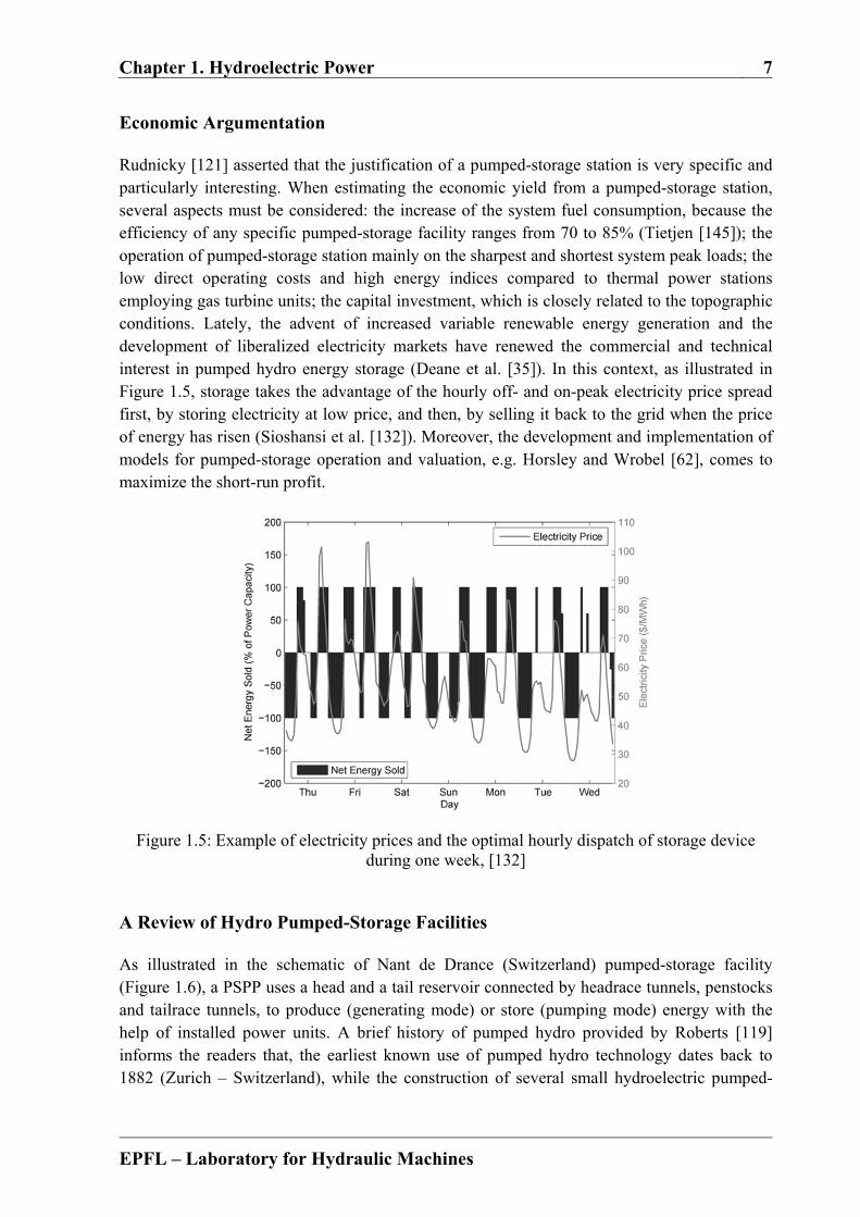
Rudnicky [121] asserted that the justification of a pumped-storage station is very specific and particularly interesting. When estimating the economic yield from a pumped-storage station, several aspects must be considered: the increase of the system fuel consumption, because the efficiency of any specific pumped-storage facility ranges from 70 to 85% (Tietjen [145]); the operation of pumped-storage station mainly on the sharpest and shortest system peak loads; the low direct operating costs and high energy indices compared to thermal power stations employing gas turbine units; the capital investment, which is closely related to the topographic conditions. Lately, the advent of increased variable renewable energy generation and the development of liberalized electricity markets have renewed the commercial and technical interest in pumped hydro energy storage (Deane et al. [35]). In this context, as illustrated in Figure 1.5, storage takes the advantage of the hourly off- and on-peak electricity price spread first, by storing electricity at low price, and then, by selling it back to the grid when the price of energy has risen (Sioshansi et al. [132]). Moreover, the development and implementation of models for pumped-storage operation and valuation, e.g. Horsley and Wrobel [62], comes to maximize the short-run profit.
Figure 1.5: Example of electricity prices and the optimal hourly dispatch of storage device during one week, [132]
A Review of Hydro Pumped-Storage Facilities
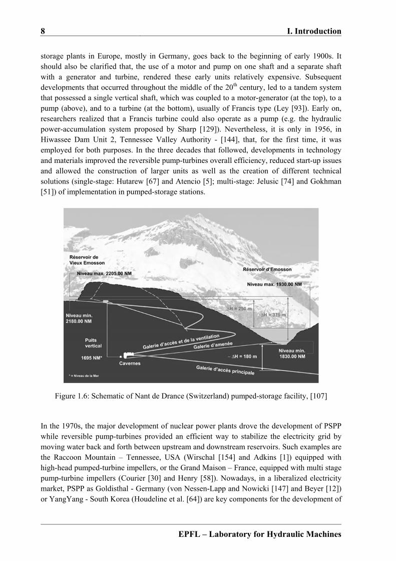
As illustrated in the schematic of Nant de Drance (Switzerland) pumped-storage facility (Figure 1.6), a PSPP uses a head and a tail reservoir connected by headrace tunnels, penstocks and tailrace tunnels, to produce (generating mode) or store (pumping mode) energy with the help of installed power units. A brief history of pumped hydro provided by Roberts [119] informs the readers that, the earliest known use of pumped hydro technology dates back to 1882 (Zurich – Switzerland), while the construction of several small hydroelectric pumped-
8 I. Introduction
EPFL – Laboratory for Hydraulic Machines
storage plants in Europe, mostly in Germany, goes back to the beginning of early 1900s. It should also be clarified that, the use of a motor and pump on one shaft and a separate shaft with a generator and turbine, rendered these early units relatively expensive. Subsequent developments that occurred throughout the middle of the 20th century, led to a tandem system that possessed a single vertical shaft, which was coupled to a motor-generator (at the top), to a pump (above), and to a turbine (at the bottom), usually of Francis type (Ley [93]). Early on, researchers realized that a Francis turbine could also operate as a pump (e.g. the hydraulic power-accumulation system proposed by Sharp [129]). Nevertheless, it is only in 1956, in Hiwassee Dam Unit 2, Tennessee Valley Authority - [144], that, for the first time, it was employed for both purposes. In the three decades that followed, developments in technology and materials improved the reversible pump-turbines overall efficiency, reduced start-up issues and allowed the construction of larger units as well as the creation of different technical solutions (single-stage: Hutarew [67] and Atencio [5]; multi-stage: Jelusic [74] and Gokhman [51]) of implementation in pumped-storage stations.
Figure 1.6: Schematic of Nant de Drance (Switzerland) pumped-storage facility, [107] In the 1970s, the major development of nuclear power plants drove the development of PSPP while reversible pump-turbines provided an efficient way to stabilize the electricity grid by moving water back and forth between upstream and downstream reservoirs. Such examples are the Raccoon Mountain – Tennessee, USA (Wirschal [154] and Adkins [1]) equipped with high-head pumped-turbine impellers, or the Grand Maison – France, equipped with multi stage pump-turbine impellers (Courier [30] and Henry [58]). Nowadays, in a liberalized electricity market, PSPP as Goldisthal - Germany (von Nessen-Lapp and Nowicki [147] and Beyer [12]) or YangYang - South Korea (Houdeline et al. [64]) are key components for the development of
Chapter 1. Hydroelectric Power 9
EPFL – Laboratory for Hydraulic Machines
new renewable CO2-free primary energies (e.g. wind or solar energy). Moreover, the most part of PSPP market is covered by reversible pump-turbines of centrifugal type with a large range of head values, from low, e.g. Alqueva - Portugal (Lavigne et al. [89]), to ultrahigh, e.g. Kazunogawa - Japan (Ikeda et al. [69]). However, seven new large pumped-storage projects under construction in Europe, Africa and Asia, that are expected to be operating by 2015 and to provide more than 4’100 MW electrical capacity (Ingram [70]), show the trend of this branch of electrical grid, thus making way even to more challenging energy storage conditions, such as using the seawater (Fujihara et al. [49]), or to futuristic projects, such as the energy island proposed by de Boer et al. [34].
1.2 Hydraulic Turbomachines
1.2.1 Hydraulic Runners Classification
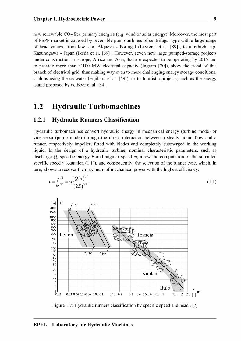
Hydraulic turbomachines convert hydraulic energy in mechanical energy (turbine mode) or vice-versa (pump mode) through the direct interaction between a steady liquid flow and a runner, respectively impeller, fitted with blades and completely submerged in the working liquid. In the design of a hydraulic turbine, nominal characteristic parameters, such as discharge Q, specific energy E and angular speed ω, allow the computation of the so-called specific speed ν (equation (1.1)), and consequently, the selection of the runner type, which, in turn, allows to recover the maximum of mechanical power with the highest efficiency.
1 21 2
3 43 42
Q
E
(1.1)
Figure 1.7: Hydraulic runners classification by specific speed and head , [7]

10 I. Introduction
EPFL – Laboratory for Hydraulic Machines
The diagram illustrated in Figure 1.7 presents the appropriate operating range that induces the best efficiency operating condition of the power unit, for each of the four main runner types, Pelton, Francis, Kaplan and Bulb respectively. Depending on the way in which the hydraulic energy is converted in mechanical energy, the hydraulic machines are divided either in impulse or reaction machines. In impulse turbines of Pelton type, which are generally used for high head and low discharge applications, one or more injectors convert the potential energy of the head into kinetic energy in the shape of water jet that acts on buckets and drives the turbine wheel. In reaction turbines such as Francis, Kaplan and Bulb, appropriate for medium and small head and medium and large discharge applications, the axial momentum of the flow is first converted in angular momentum with the help of the guide vanes, and then recovered as mechanical torque, by the runner blades, through the flow deviation.
1.2.2 Francis-Type Reversible Pump-Turbine
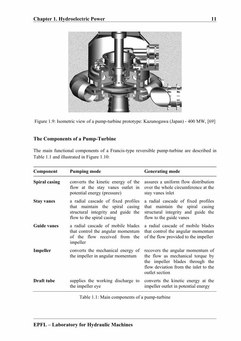
The Francis turbine was invented in the 19th century by the American engineer James B. Francis. It is a reaction machine that combines both radial and axial flow concepts, that is appropriate for head range of 20 m ÷ 700 m, and that reaches an output power from few kilowatts up to one gigawatt, with efficiency greater than 90%. The impeller of centrifugal pumps converts the mechanical power into hydraulic energy (pressure), and since its design is similar to the one of the Francis runner, in the particular case of reversible pump-turbines it may be also used to produce mechanical energy. The appropriate operating range of a Francis-type reversible pump-turbine depending on the head and specific speed is provided in Figure 1.8. Thus, the low specific speed and high head pump-turbines, as the one illustrated in Figure 1.9, are characterized by a narrow shape of impeller channels at the inlet section in turbine mode, whereas the impellers of high specific speed and low head machines, feature large impeller channels width at the inlet section.
Figure 1.8: Francis-type reversible pump-turbine impeller shape by specific speed, [7]
Chapter 1. Hydroelectric Power 11
EPFL – Laboratory for Hydraulic Machines
Figure 1.9: Isometric view of a pump-turbine prototype: Kazunogawa (Japan) - 400 MW, [69]
The Components of a Pump-Turbine
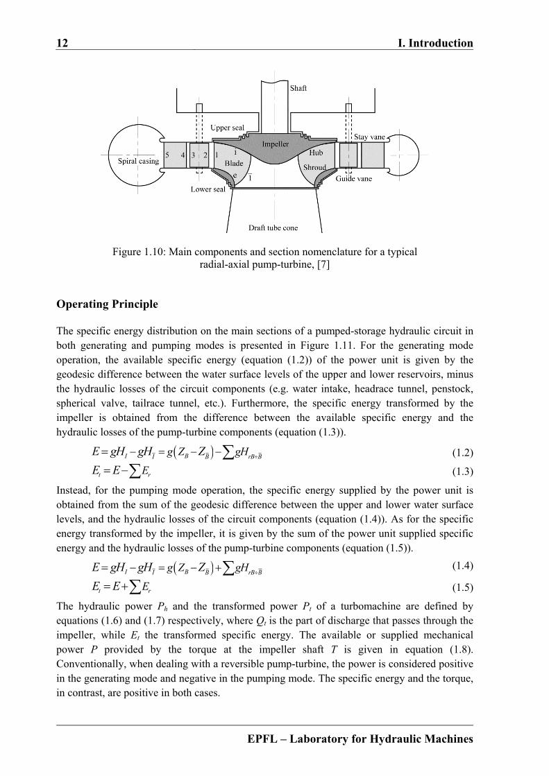
The main functional components of a Francis-type reversible pump-turbine are described in Table 1.1 and illustrated in Figure 1.10:
Component Pumping mode Generating mode
Spiral casing converts the kinetic energy of the flow at the stay vanes outlet in potential energy (pressure)
assures a uniform flow distribution over the whole circumference at the stay vanes inlet
Stay vanes a radial cascade of fixed profiles that maintain the spiral casing structural integrity and guide the flow to the spiral casing
a radial cascade of fixed profiles that maintain the spiral casing structural integrity and guide the flow to the guide vanes
Guide vanes a radial cascade of mobile blades that control the angular momentum of the flow received from the impeller
a radial cascade of mobile blades that control the angular momentum of the flow provided to the impeller
Impeller converts the mechanical energy of the impeller in angular momentum
recovers the angular momentum of the flow as mechanical torque by the impeller blades through the flow deviation from the inlet to the outlet section
Draft tube supplies the working discharge to the impeller eye
converts the kinetic energy at the impeller outlet in potential energy
Table 1.1: Main components of a pump-turbine
12 I. Introduction
EPFL – Laboratory for Hydraulic Machines
Figure 1.10: Main components and section nomenclature for a typical radial-axial pump-turbine, [7]
Operating Principle
The specific energy distribution on the main sections of a pumped-storage hydraulic circuit in both generating and pumping modes is presented in Figure 1.11. For the generating mode operation, the available specific energy (equation (1.2)) of the power unit is given by the geodesic difference between the water surface levels of the upper and lower reservoirs, minus the hydraulic losses of the circuit components (e.g. water intake, headrace tunnel, penstock, spherical valve, tailrace tunnel, etc.). Furthermore, the specific energy transformed by the impeller is obtained from the difference between the available specific energy and the hydraulic losses of the pump-turbine components (equation (1.3)).
I BI B rB Bg Z gHE gH gH Z (1.2)
t rEE E (1.3)
Instead, for the pumping mode operation, the specific energy supplied by the power unit is obtained from the sum of the geodesic difference between the upper and lower water surface levels, and the hydraulic losses of the circuit components (equation (1.4)). As for the specific energy transformed by the impeller, it is given by the sum of the power unit supplied specific energy and the hydraulic losses of the pump-turbine components (equation (1.5)).
I BI B rB Bg Z gHE gH gH Z (1.4)
t rEE E (1.5)
The hydraulic power Ph and the transformed power Pt of a turbomachine are defined by equations (1.6) and (1.7) respectively, where Qt is the part of discharge that passes through the impeller, while Et the transformed specific energy. The available or supplied mechanical power P provided by the torque at the impeller shaft T is given in equation (1.8). Conventionally, when dealing with a reversible pump-turbine, the power is considered positive in the generating mode and negative in the pumping mode. The specific energy and the torque, in contrast, are positive in both cases.

Chapter 1. Hydroelectric Power 13
EPFL – Laboratory for Hydraulic Machines
Figure 1.11: Specific energy distribution in generating and pumping modes, [7]
0, 0, 0 Turbine mode
0, 0, 0 Pump mode, h
hh
P Q E
P Q EP Q E
(1.6)
0, 0, 0 Turbine mode
0, 0, 0 Pump mode, t t t
t t tt t t
P Q E
P Q EP Q E
(1.7)
0, 0, 0 Turbine mode
0, 0, 0 Pump mode,
P T
P TP T
(1.8)
Finally, the global efficiency η of the power unit is given by equation (1.9) as a result of the product between the bearing efficiency ηm and the hydraulic efficiency ηh expressed by equation (1.10), which includes the efficiency of the disc friction ηrm, the energetic efficiency ηe as well as the volumetric efficiency ηq.
, Turbine mode
, Pump modeh
h mh
P P
P P
(1.9)
The operation of a power unit in the whole range, either in the generating or pumping mode, is guided by the so-called efficiency hill chart obtained through the superposition of the efficiency on the characteristic curves. Thus, the dimensionless speed, discharge and torque

14 I. Introduction
EPFL – Laboratory for Hydraulic Machines
, Turbine mode
, Pump mode
t trm
h rm e q
rmt t
E Q
E Q
E Q
E Q
(1.10)
factors, which are expressed by equations (1.11) - (1.13) according to IEC 60193 standards [71], can be used to draw the QED(nED) and TED(nED) characteristic curves of a prototype for different constant guide vanes openings. As far as the efficiency is concerned, while mechanical and disk friction losses are predictable for a large range of operation, the viscous dissipation losses depend on the complex tridimensional flow, and so model testing is required for a precise evaluation.
1 Speed FactoreED
E
n Dn
(1.11)
21
Discharge FactorED
eD E
(1.12)
31
Torque FactorED
eD E
TT
(1.13)
Velocity Triangles
For the characterization of the flow inside the impeller, two reference frames, an absolute Cartesian one and a relative cylindrical one respectively, are considered (see Figure 1.12).
Thus, according to equation (1.14), the absolute flow velocity of any point in the impeller
can be decomposed in a circumferential component (equation (1.15)) and in a relative
component . Moreover, the projection of the absolute velocity on a meridional plane gives
the meridional velocity , whereas the projection on tangential direction gives the peripheral
absolute velocity .
U WC
(1.14)
U R e
(1.15)
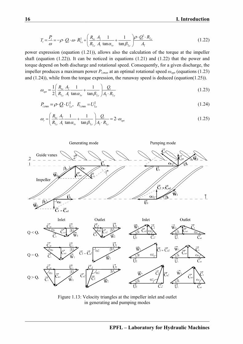
The velocity triangles at the inlet and outlet of the impeller in both turbine and pump modes for the best efficiency, part- and full load operating points, are illustrated in Figure 1.13. The β angle is given by the relative flow velocity, perfectly adapted to both leading and trailing edge of the impeller blade at BEP. The α angle is given by the absolute velocity of the flow, which is aligned with the guide vanes profiles at the impeller inlet (turbine mode) and outlet (pump mode) respectively. In the case of a pump-turbine, at the BEP (nominal discharge), the velocity triangle at the impeller inlet in turbine mode or outlet in pump mode, is isosceles, while at the impeller outlet (turbine mode) and inlet (pump mode), it exhibits an axial flow. In contrast, it can be observed that the part- and full load operations are characterized by the presence of a residual positive or negative peripheral absolute velocity at the impeller outlet/inlet (turbine/pump mode), which is responsible for the development of the so-called helical and respectively axisymmetric vortex ropes in the draft tube cone.

Chapter 1. Hydroelectric Power 15
EPFL – Laboratory for Hydraulic Machines
Figure 1.12: Flow velocity vectors representation into a Francis-type runner, [7] & [18] The local form of linear Euler energy-discharge characteristic equation for the transformed
specific energy Et between the impeller inlet (1) and outlet (1) sections is given by equation (1.16), considering a streamline near the shroud (e). According to velocity triangles, the peripheral absolute velocity Cu can be calculated using the meridional velocity and the absolute and relative flow angles (equation (1.17)). Moreover, the meridional velocity can be obtained from the transformed discharge Qt and the flow distribution coefficient kCm by applying the equation (1.18). Thereby, the expression of transformed energy depending only on the absolute flow angle, impeller outlet blade angle, discharge and rotational speed is provided by equation (1.19).
1 1 1 1 1 1t Cu e u e e Cu e u e eC U C UE k k (1.16)
1 11 1 1
1 1
,tan tan
m e m eu e u e e
e e
CCC C U
(1.17)
1 11 1 1 1
,t tm e m e
Cm e Cm e
Q QC C
k A k A
(1.18)
2 1 1 1 111 1
1 1 11 1 1 1
1 1
tan tantCu e e Cu e e
t Cu e eCm e ee Cm e e
Q UARU
R A A
kkE k
k k
(1.19)
In generating mode, when is assumes a uniform flow distribution at the impeller inlet and outlet, of Cu and Cm from the hub to the shroud, the transformed specific energy takes the simplified form expressed in equation (1.20), which, when introduced in the transformed
2 1 111
1 11 1 1
1 1
tan tante e
t eee e
Q UARU
R A AE
(1.20)
22 1 111
1 11 1 1
1 1
tan tante e
t t t t eee e
Q UARP U
R A AQ E Q
(1.21)
16 I. Introduction
EPFL – Laboratory for Hydraulic Machines
22 1 111
1 11 1 1
1 1
tan tantt e e
t t eee e
Q RART
R A A
PQ R
(1.22)
power expression (equation (1.21)), allows also the calculation of the torque at the impeller shaft (equation (1.22)). It can be noticed in equations (1.21) and (1.22) that the power and torque depend on both discharge and rotational speed. Consequently, for a given discharge, the impeller produces a maximum power Pt,max at an optimal rotational speed ωopt (equations (1.23) and (1.24)), while from the torque expression, the runaway speed is deduced (equation(1.25)).
1 1
1 11 1 1 1
1 1
2 tan tan
1 e topt
ee e e
AR Q
R A A R
(1.23)
2 2,max ,max1 1,t t te eP U E UQ (1.24)
1 1
1 11 1 1 1
1 1
tan tan2e t
r optee e e
AR Q
R A A R
(1.25)
Figure 1.13: Velocity triangles at the impeller inlet and outlet in generating and pumping modes
Chapter 1. Hydroelectric Power 17
EPFL – Laboratory for Hydraulic Machines
In the pumping mode operation, the transformed specific energy may be expressed through equation (1.26) when a uniform flow distribution at the impeller inlet and outlet as well as an axial flow at the impeller inlet are considered. The peripheral absolute velocity and the meridional velocity can be calculated by using the velocity triangle at the impeller outlet section on an external streamline, as expressed in equation (1.27).
1 11 1 02
1, 1,Cu Cm t u e eu ek k C E C U (1.26)
11 1 1
1 1
,tan
m e tu e e m e
e
C QC U C
A (1.27)
When the expanded form of the transformed specific energy (equation (1.28)) is introduced in the transformed power expression (equation (1.29)), the transformed torque at the impeller shaft can be expressed as in equation (1.30).
2 11
1 1
1
tant e
t ee
Q UU
AE
(1.28)
22 11
1 1
1
tant e
t t t t ee
Q UP U
AQ E Q
(1.29)
22 11
1 1
1
tanRt t e
t t ee
Q RT
A
PQ
(1.30)
Consequently, for a given rotational speed, for an optimum discharge Qt (equation (1.31)), the impeller can provide a maximum power and energy, given in equation (1.32). Finally, the discharge at runaway operation may be obtained from the torque expression (equation (1.33)).
1 1 1tan2
1opt e eQ U A (1.31)
2 21 1
,max ,max,2 2
e et t t
U UP EQ (1.32)
1 1 1tan 2r e e optQ U A Q (1.33)

EPFL – Laboratory for Hydraulic Machines
Chapter 2
Case Study
2.1 Four Quadrants Operation
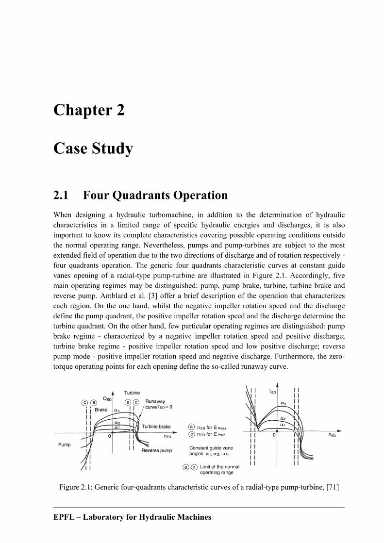
When designing a hydraulic turbomachine, in addition to the determination of hydraulic characteristics in a limited range of specific hydraulic energies and discharges, it is also important to know its complete characteristics covering possible operating conditions outside the normal operating range. Nevertheless, pumps and pump-turbines are subject to the most extended field of operation due to the two directions of discharge and of rotation respectively - four quadrants operation. The generic four quadrants characteristic curves at constant guide vanes opening of a radial-type pump-turbine are illustrated in Figure 2.1. Accordingly, five main operating regimes may be distinguished: pump, pump brake, turbine, turbine brake and reverse pump. Amblard et al. [3] offer a brief description of the operation that characterizes each region. On the one hand, whilst the negative impeller rotation speed and the discharge define the pump quadrant, the positive impeller rotation speed and the discharge determine the turbine quadrant. On the other hand, few particular operating regimes are distinguished: pump brake regime - characterized by a negative impeller rotation speed and positive discharge; turbine brake regime - positive impeller rotation speed and low positive discharge; reverse pump mode - positive impeller rotation speed and negative discharge. Furthermore, the zero-torque operating points for each opening define the so-called runaway curve.
Figure 2.1: Generic four-quadrants characteristic curves of a radial-type pump-turbine, [71]

20 I. Introduction
EPFL – Laboratory for Hydraulic Machines
When operating in the generating mode, the machine is put, during the start-up procedure, in runaway operation (speed no-load condition) prior to its synchronization. Depending on the specific speed of the pump-turbine, the discharge-speed as well as torque-speed characteristics at constant guide vanes opening can be “S-shaped” featuring positive slope (see Figure 2.2). The main issue with such a characteristic curve is that, at runaway, the machine may switch back and forth from generating to reverse pumping modes. Moreover, it is well known that such unstable operation leads to a significant increase in structural vibrations and noise.
Figure 2.2: “S-shaped” characteristic curves of a pump-turbine in generating mode, [53] Early studies reported the technical challenges of pump-turbines operation under unsteady off-design regimes (Blanchon et al. [14], Casacci et al. [25] and Lacoste [86]). Borciani and Thalmann [16] performed an experimental study of the influence of cavitation on average and instantaneous characteristics of turbines and pump-turbines. Their results show that not only may the operation Thoma number σ affect the normal operating range but it may also change the characteristic shape in the turbine brake and in the reverse pump region. In addition to this, few authors (Taulan [143], Pejovic et al. [115], Tanaka and Tsunoda [141], Oishi and Yokoyama [112]) investigated the unsteady phenomena that could develop in a pump-turbine during sudden load rejection. Martin [98] & [99] proposed a stability analysis to predict the occurrence of large flow oscillations for idealized machine arguing that the unstable operation in case of load-rejection with failed servomotor is mainly attributable to the presence of a positive slope on the torque characteristic at runaway. Nicolet [110] stated that high head pump-turbines, which are common characteristic of low specific speeds, are more subjected to “S-shaped” characteristic curves. Furthermore, Calendray et al. [24], Nicolet et al. [109] and Widmer et al. [151] performed numerical analyses of the unstable behavior of a pump-turbine operating at runaway and/or in turbine brake mode. Interestingly, Dörfler [39] proposed an improvement of the torque characteristic representation that might be useful for expressing other mechanical parameters of the machine. Since the impeller of a reversible pump-turbine is mainly designed for pump mode operation, as specified by Stelzer and Walters [137] or Nowicki et al. [111], the utilization of centrifugal pumps as turbines with the aim of generating electricity, becomes sometimes justified. Mankbadi and Mikhail [97] as well as Derakhshan and Nourbakhsh [37] developed methods that can be employed to estimate the turbine mode operating characteristics for such cases.
Chapter 2. Case Study 21
EPFL – Laboratory for Hydraulic Machines
Nevertheless, it should be kept in mind that, during the optimization process, both pump and turbine regimes must be considered. Billdal and Wedmark [13] claimed that, in practice, a single-stage reversible pump-turbine is by nature forced to be operated as a compromise between an optimum pump and an optimum turbine. In order to obtain the advantages of a simplified and cost-effective pump-storage design concept, some penalty has to be paid on the overall performance. The main reason for this is the following: because of the fact that the optimum speed is not the same in turbine and pump mode, and the speed is governed by the pump performance, the turbine is operating at off-design conditions in the whole operational domain. Recently, Staubli et al. [136] performed a numerical investigation of the flow in a pump-turbine operating nearby runaway condition. They concluded that local vortices, formed at the inlet of the impeller channels, represent the source of the unsteady in- and outflow from the impeller in the vaneless gap between the impeller and the guide vanes. Further, Wang et al. [149] argued that the dominant vortex located near the runner inlet leads to the speed-no-load instability. Liang et al. [94] also ran an unsteady flow simulation at the speed no-load condition for two pump-turbine reduced models, finding out that the impeller inlet operates as a pump with negative blade loading, whereas the impeller outlet operates as a turbine with positive blade loading - the equilibrium between the pumping and generating loads conducts to zero torque at the shaft. Moreover, the interaction between inflow and backflow at the impeller inlet renders the local flow field very complex. Nevertheless, few technical solutions to stabilize the machine during the start-up or in case of a sudden load rejection are reported in the literature. Huvet [68] marked out charts to enable the designer as well as the operator to assess the steady oscillatory conditions. Dörfler et al. [40] proposed an interesting method that can be used in order to avoid unstable operation of pump-turbines during model tests - the inlet valve is partially opened and by-passed with a second valve so as to adjust the flow rate. The resulting artificial head loss improves significantly the hydraulic stability. Kuwabara et al. [85] developed an advanced control of the guide vane independent servomotors, which was provided with an anti-S-characteristics control to be used upon load rejection. Klemm [80] reported the implementation of the Misaligned Guide Vanes (MGV) concept in the COO II pumped-storage power plant in Belgium, in order to achieve an improvement of the machine stability for no-load and extreme part-load conditions. As presented also by Bouschon et al. [17], this method consists in operating several guide vanes that are independent from the rest of the guide vane mechanism by using independent servomotors. This allows the operator to stabilize the machine. Recently, Shao [128] advanced and validated empirical formulae of the pump-turbine internal characteristics with MGV that are based on the internal characteristic theory of turbomachinery and the original model characteristic curves without MGV.
22 I. Introduction
EPFL – Laboratory for Hydraulic Machines
2.2 Hydrodynamic Instabilities
Rotor-Stator Interaction
During the operation of a hydraulic turbomachine at any operating point, the relative motion between the impeller blades and guide vanes induces pressure fluctuations that propagate through the entire machine (Zobeiri [158]). Liees et al. [95] stated that the periodic passing frequency of the guide vanes, when viewed from the impeller, is relatively high and frequent within the range of natural frequencies of the impeller components, and therefore it is often the source of unwished vibrations and fatigue cracks in the impeller. Indeed, the amplitude of pressure fluctuations induced by the impeller blades passage was found to be strongly influenced by the rotor-stator vaneless gap, by the shape of the impeller blades trailing edge in pumping mode (Al-Qutub et al. [2]), and as well as by the operating regime (Parrondo-Gayo et al. [113]). Moreover, through the use of experimental measurements, Tanaka [142] developed a theoretical model that allowed him to determine the diametrical vibration modes in a pump-turbine. Undoubtedly, both the experimental flow investigations, instantaneous velocity and pressure measurements mainly in the stator (e.g. Ciocan and Kueny [27]) included, and the numerical flow investigations (e.g. Zobeiri et al. [159]), available in the literature, are key points to consider when describing the mechanism and the effects of the rotor-stator interaction (RSI) phenomenon.
Flow Separation
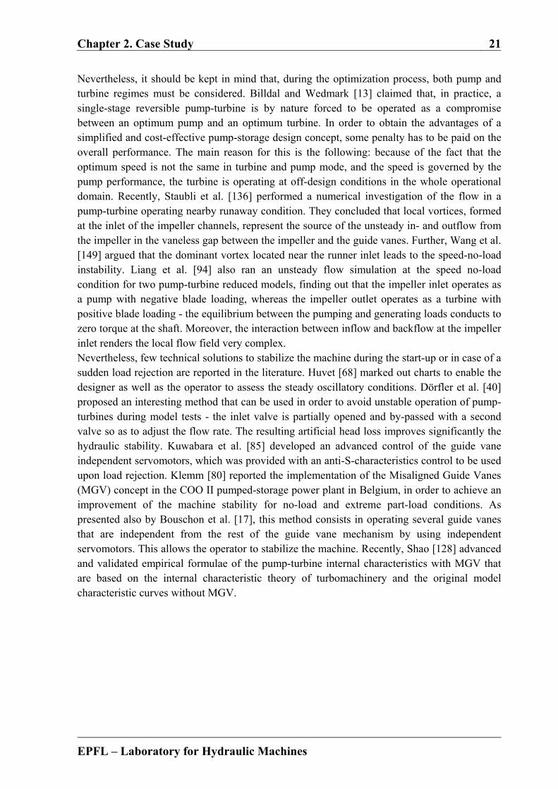
Flow separation is a complex phenomenon, which is present in the flow around an aero- or hydrofoil, at high Reynolds number, mainly when the incidence angle is changed from zero (Figure 2.3). More precisely, the flow separation begins in the boundary layer when the shear stress at the wall is equal to zero due to the flow deceleration, as described in Batchelor [9], Guyon et al. [52], Ryhming [123], and White [150]. Thus, a method to be used in order to delay or even to avoid the separation would be that of increasing the shear stress. This can be achieved by forcing, e.g. through the introduction of roughness at the wall, a turbulent boundary layer transition when the additional disturbances feed the boundary layer (Ausoni [6]). Simpson [130] defined the separation as the entire process of departure or breakaway, or the breakdown of boundary layer flow. Williams [153] was doubtful about how to handle the
Figure 2.3: Flow separation over a hydraulic profile
Chapter 2. Case Study 23
EPFL – Laboratory for Hydraulic Machines
problem within the framework of boundary-layer theory alone. Hence, he asserted that the separation point represents a boundary between two regions of vastly different scales. Furthermore, Dengel and Fernholz [36] performed an experimental investigation of an incompressible turbulent boundary layer in the vicinity of separation. Smith [133] summarized a high Reynolds number theory around the issue of separation in steady or unsteady boundary layers, while Vorus [148] formulated a high Reynolds number theory for the approximate analysis of timewise steady viscous flows. Hu and Yang [65] claimed that the flow separation generates an unsteady area with a high level of turbulence and many recirculation zones. As described by Hoarau et al. [61], another important effect of the flow separation is the generation of vortices, which is carried out through two types of mechanism: the von Karman and the Kelvin-Helmholtz instabilities respectively, both generated by the velocity shear present in the region of flow separation. Simpson [130] fond that, at the maximum lift - angle of attack (also called stall angle), the boundary-layer flow on the front third of the chord abruptly separates, inducing a catastrophic drop in the lift. Moreover, the magnitude of the reversed flow near the surface increases as the large separation vortex forms and moves downstream. If the angle of attack of an airfoil or other lifting surface oscillates around the static stall angle, large hysteresis develops forces and moments in the fluid-dynamics (McCroskey [100]). Kline [81] created a classification of the major stall types by using a qualitative parameter, and promoted the idea that the boundary layer theory is not sufficient to predict the onset or the behavior of stall. Leishman [90] concluded that static stall characteristics, such as stall type or maximum lift coefficient, are not necessarily useful indicators to show how an airfoil will behave under dynamic stall conditions. Nevertheless, when dealing with hydraulic turbomachines, the flow separation on any solid surface in the stator or rotor that usually occurs in off-design operating conditions, is one of the sources that induce flow unsteadiness and efficiency drop.
Rotating Stall
According to Frigne and Van Den Braembussche [48], the unsteady flow phenomenon that gives rise to the occurrence of subsynchronous rotating velocity fluctuations is commonly referred as “rotating stall”. Berten [11] asserted that, the so-called stall is a highly dynamic phenomenon, which can occur in impellers and/or stationary components of hydraulic machines, especially when the flow conditions yield high incidence angles at the impeller blades or diffuser vanes; further, under specific conditions, a stationary separation zone may begin to progress, this phenomenon being called rotating stall. Indeed, rotating stall manifests itself in compressible as well as incompressible flows (Stenning [138]). Emmons et al. [43] provided researchers with a first literature review along with a simplified mathematical model to predict the stall propagation in idealized compressor. Chen et al. [26] showed that, a mechanism similar to the mid-latitude wind system in the Earth’s atmosphere, dominated by Rossby waves and their associated circular Karman vortex streets, govern the development of rotating stall in the impeller of an axial or radial turbocompressor. Ljevar et al. [96] carried out a numerical study on the vaneless diffuser core flow instability in centrifugal compressors, and concluded that the flow mechanism of a rotating stall is strongly influenced by the diffuser
24 I. Introduction
EPFL – Laboratory for Hydraulic Machines
geometry as well as by the inlet and outlet flow conditions. Using pressure measurements, Stepanik and Brekke [139] detected the presence of a rotating stall in the stator of a pump-turbine reduced scale model under part load operating conditions in pump mode. Johnson et al. [75] performed complementary LDV and pressure measurements in the impeller of a centrifugal pump at reduced flow off-design conditions, and detected the presence of stationary stable stall cells in alternate impeller channels. Sano et al. [125] investigated numerically the flow instabilities in a pump vaned diffuser, claiming that the rotating stall onset flow rate is larger in case of a larger vaneless gap. Dixon [38] and Brennen [22] described the stall propagation phenomenon in a stator or rotor pump blades, whereas Fay [46] presented the mechanism of the stall propagation in case of a turbine cascade. Thus, considering three consecutive stator/impeller blades operating at large incidence angle, a perturbation of the incoming flow (e.g. the rotor-stator interaction) induces a stall in one of the channels. Furthermore, the blockage induces an increase of the incidence angle for the follower blade as well as a decrease of the incidence angle for the forerunner blade. Hence, the stall moves on a direction away from the incoming flow. Indeed, the stall cell can occur on several consecutive channels and/or several simultaneous points on the circumference. In the case of a rotor, the stall rotates in the same direction with the impeller, but with 50–70% of its angular velocity - e.g. the rotating stall developed in the impeller of a pump-turbine scale model operating in turbine brake mode, Widmer et al. [152].

EPFL – Laboratory for Hydraulic Machines
Chapter 3
Overview of Current Work
3.1 Problematic and Objective
Problematic
In order to compensate the random nature of consumption, major development of thermal power generators – either coal or nuclear – within a power generation mix, requires the construction of pumped-storage power plants. This compensation is achieved by storing energy in excess or delivering peak energy, which, in turn, permits to meet the demand. Therefore, by moving water back and forth between upstream and downstream reservoirs, reversible pump-turbines provide an efficient way to stabilize the electricity grid. Nowadays, in a context of liberalized electricity market, pumped-storage power plants are key components for the development of new renewable CO2-free primary energies (e.g. wind or solar energy). Moreover, since the electricity network frequency must be maintained stable, the pump-turbines are subject to a rapid switching between the pumping and generating modes with extended operation under off-design conditions. In particular, during the start-up procedure, the machine is put in runaway operation (speed no-load condition) prior to its synchronization. Depending on the specific speed of the pump-turbine, the discharge-speed as well as torque-speed characteristics at constant guide vanes opening can be “S-shaped”, featuring positive slope. The main issue with such a characteristic curve might be that the machine operation becomes strongly unstable at runaway speed and beyond, switching back and forth from generating to reverse pumping modes, the synchronization with the electrical network in safety conditions becoming impossible. Furthermore, it is well known that such unstable operation leads to a significant increase of structural vibrations.
26 I. Introduction
EPFL – Laboratory for Hydraulic Machines
Objective
The present study is focused on the hydrodynamics of a low specific speed radial pump-turbine reduced scale model at off-design operation in generating mode, experiencing unstable operating conditions (positive slope) at runaway. A complementary experimental and numerical approach is adopted to identify and describe the onset and the development of flow instabilities when the machine is brought from the best efficiency point (BEP) to runaway and turbine brake mode. In particular, a comparative study is performed between the normal operating range, runaway and very low positive discharge operating conditions at 10° guide vanes opening angle. Discovery experiments involve high-speed flow visualizations, either tuft or injected air bubbles, PIV measurements in the stator, and wall pressure measurements in both rotating and stationary frames. The unsteady incompressible turbulent flow numerical simulation is performed in the full reduced scale model water passage domain using the Ansys CFX code for the selected operating points. The incompressible unsteady Reynolds-Averaged Navier-Stokes equations are solved by using the finite volume method. Wall pressure measurements in both rotating and stationary frames are used to validate the numerical results. Having said that, the current study exploits the advantages of the numerical simulation in order to investigate the flow instabilities development mainly in the rotating frame, which is a context where, if considered experimentally, the measurements are too expensive or technically limited in terms of time and costs even in a reduced scale model.
3.2 Document Organization
The thesis has been structured into five parts, as follows:
Part I offers an introduction about the pumped-storage technology in the general context of electrical grid and the hydraulic turbomachines operation principle. In addition to this, this section makes readers familiar with the Francis-type reversible pump-turbines technical challenges along with the objectives of the current study.
Part II concerns the investigation methodology, including the experimental instrumentation setup and the numerical modeling. The pressure instrumentation in both stationary and rotating frames, the PIV system, as well as the employed high-speed visualization techniques are first detailed. Follows a discussion about the numerical modeling elements, such as the governing equations, the turbulence model choice, the numerical scheme, the computational domain, the spatial discretization and the boundary conditions
Part III presents the experimental measurements results. The onset and the development of flow instabilities in situations where the machine is brought from the best efficiency point (BEP) to runaway and turbine brake mode are experimentally evidenced. This is achieved by using the measurements of pressure fluctuations at the wall in both stator and rotor, high-speed flow visualizations - either tuft or injected air bubbles - as well as velocity measurements in the vaneless space between the impeller and guide vanes. The relationship between the presence of positive slope on the characteristic and the development of rotating stall are investigated as well.

Chapter 3. Overview of Current Work 27
EPFL – Laboratory for Hydraulic Machines
Part IV deals with the numerical simulation results. Once the numerical simulation is validated, a comparative study is conducted between the normal operating range, runaway and very low positive discharge operating conditions at 10° guide vanes opening angle. The onset of rotating stall at the runaway condition is evidenced. Finally, the mechanism of rotating stall onset and development when operating a pump-turbine at off-design conditions in generating mode is discussed.
Part V draws concluding remarks and suggests future investigation directions.


EPFL – Laboratory for Hydraulic Machines
Part II
Investigation Methodology


EPFL – Laboratory for Hydraulic Machines
Chapter 4
Experimental Instrumentation Setup
4.1 Reversible Pump-Turbine Scale Model
The flow hydrodynamics in the reduced scale model of a low specific speed Francis-type reversible pump-turbine (Table 4.1 and Figure 4.1), experiencing unstable operation at runaway condition, is experimentally and numerically investigated at off-design conditions in generating mode. This study, which is part of the “Hydrodyna” collaborative research project that was conducted by the Laboratory for Hydraulic Machines from EPFL in collaboration with the world major pump-turbine manufacturers, aims at developing a methodology for engineering safe pump-turbines that meets the challenging requirements of the hydropower market.
Figure 4.1: Hydrodyna pump-turbine reduced scale model

32 II. Investigation Methodology
EPFL – Laboratory for Hydraulic Machines
Parameter Description Value
Specific speed 0.17 Number of impeller blades 9 Number of guide vanes 20
Impeller inlet diameter 523.5 mm
Impeller outlet diameter 250 mm
Nominal guide vanes opening 18°
Nominal discharge coefficient 0.36
Nominal energy coefficient 0.54
Table 4.1: Summary of the main pump-turbine scale model parameters - turbine mode
4.2 Model Testing Facilities
Test Rigs
An experimental flow investigation in the pump-turbine reduced scale model operating at off-design conditions in generating mode is performed in several sessions. The model is installed in two of the EPFL-LMH hydraulic machines testing facilities, PF2 and PF3 respectively, as illustrated in Figure 4.2 and Figure 4.3.
Figure 4.2: Model installation scheme in the EPFL PF2 and PF3 testing facilities
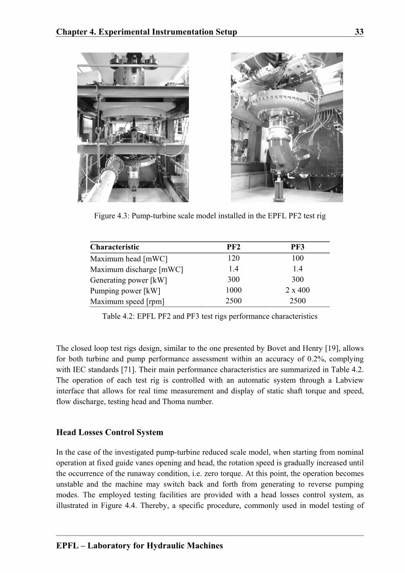
Chapter 4. Experimental Instrumentation Setup 33
EPFL – Laboratory for Hydraulic Machines
Figure 4.3: Pump-turbine scale model installed in the EPFL PF2 test rig
Characteristic PF2 PF3
Maximum head [mWC] 120 100
Maximum discharge [mWC] 1.4 1.4
Generating power [kW] 300 300
Pumping power [kW] 1000 2 x 400
Maximum speed [rpm] 2500 2500
Table 4.2: EPFL PF2 and PF3 test rigs performance characteristics The closed loop test rigs design, similar to the one presented by Bovet and Henry [19], allows for both turbine and pump performance assessment within an accuracy of 0.2%, complying with IEC standards [71]. Their main performance characteristics are summarized in Table 4.2. The operation of each test rig is controlled with an automatic system through a Labview interface that allows for real time measurement and display of static shaft torque and speed, flow discharge, testing head and Thoma number.
Head Losses Control System
In the case of the investigated pump-turbine reduced scale model, when starting from nominal operation at fixed guide vanes opening and head, the rotation speed is gradually increased until the occurrence of the runaway condition, i.e. zero torque. At this point, the operation becomes unstable and the machine may switch back and forth from generating to reverse pumping modes. The employed testing facilities are provided with a head losses control system, as illustrated in Figure 4.4. Thereby, a specific procedure, commonly used in model testing of
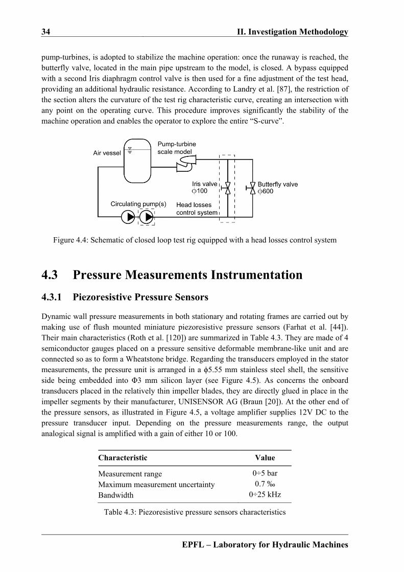
34 II. Investigation Methodology
EPFL – Laboratory for Hydraulic Machines
pump-turbines, is adopted to stabilize the machine operation: once the runaway is reached, the butterfly valve, located in the main pipe upstream to the model, is closed. A bypass equipped with a second Iris diaphragm control valve is then used for a fine adjustment of the test head, providing an additional hydraulic resistance. According to Landry et al. [87], the restriction of the section alters the curvature of the test rig characteristic curve, creating an intersection with any point on the operating curve. This procedure improves significantly the stability of the machine operation and enables the operator to explore the entire “S-curve”.
Figure 4.4: Schematic of closed loop test rig equipped with a head losses control system
4.3 Pressure Measurements Instrumentation
4.3.1 Piezoresistive Pressure Sensors
Dynamic wall pressure measurements in both stationary and rotating frames are carried out by making use of flush mounted miniature piezoresistive pressure sensors (Farhat et al. [44]). Their main characteristics (Roth et al. [120]) are summarized in Table 4.3. They are made of 4 semiconductor gauges placed on a pressure sensitive deformable membrane-like unit and are connected so as to form a Wheatstone bridge. Regarding the transducers employed in the stator measurements, the pressure unit is arranged in a ϕ5.55 mm stainless steel shell, the sensitive side being embedded into Φ3 mm silicon layer (see Figure 4.5). As concerns the onboard transducers placed in the relatively thin impeller blades, they are directly glued in place in the impeller segments by their manufacturer, UNISENSOR AG (Braun [20]). At the other end of the pressure sensors, as illustrated in Figure 4.5, a voltage amplifier supplies 12V DC to the pressure transducer input. Depending on the pressure measurements range, the output analogical signal is amplified with a gain of either 10 or 100.
Characteristic Value
Measurement range 0÷5 bar
Maximum measurement uncertainty 0.7 ‰
Bandwidth 0÷25 kHz
Table 4.3: Piezoresistive pressure sensors characteristics

Chapter 4. Experimental Instrumentation Setup 35
EPFL – Laboratory for Hydraulic Machines
Figure 4.5: Miniature piezoresistive pressure sensor and the electronic connection scheme with the amplifier for measurements in the stator
Pressure Sensors Calibration
The static calibration of the pressure transducers is performed by using a pressurized vessel partially filled with water in which the sensors are flush mounted, the experimental setup for both stationary and rotating frames sensors calibration being illustrated in Figure 4.6. Conditioning electronics identical to those used during the measurements on the test rig are considered. To achieve the sensors calibration parameter (pressure/voltage slope), the pressure is gradually increased from the atmospheric one to about 6 bars, and then reduced back to the atmospheric pressure. Voltage outputs of pressure sensors are then averaged and compared to the readings of a high precision reference pressure transducer, [66]. It should be noticed that, if one considers a linear relation between the pressure and measured voltage (equation (4.1)), the slope A1 and the intercept A0 are obtained by linear regression (equation (4.2)), with the mean reference pressure and voltage that are calculated by applying the equation (4.3).
0 1AUp A (4.1)
,1
12
1
0 1
N
i ref i refi
N
ii
ref
U U p p
U U
A p AU
A
(4.2)
,1 1
1 1and
N N
ref ref i ii i
p p U UN N
(4.3)
The relative measurement error is finally computed using the equation (4.4). Values that are below ±0.7 ‰ are usually achieved.
,max ,min
refrel
ref ref
p p
p p
(4.4)
Figure 4.7 displays typical calibration curves, which in turn show the linear slope and the error of measured against linearized values. As a result, the pressure sensor in Figure 4.7a) plot is
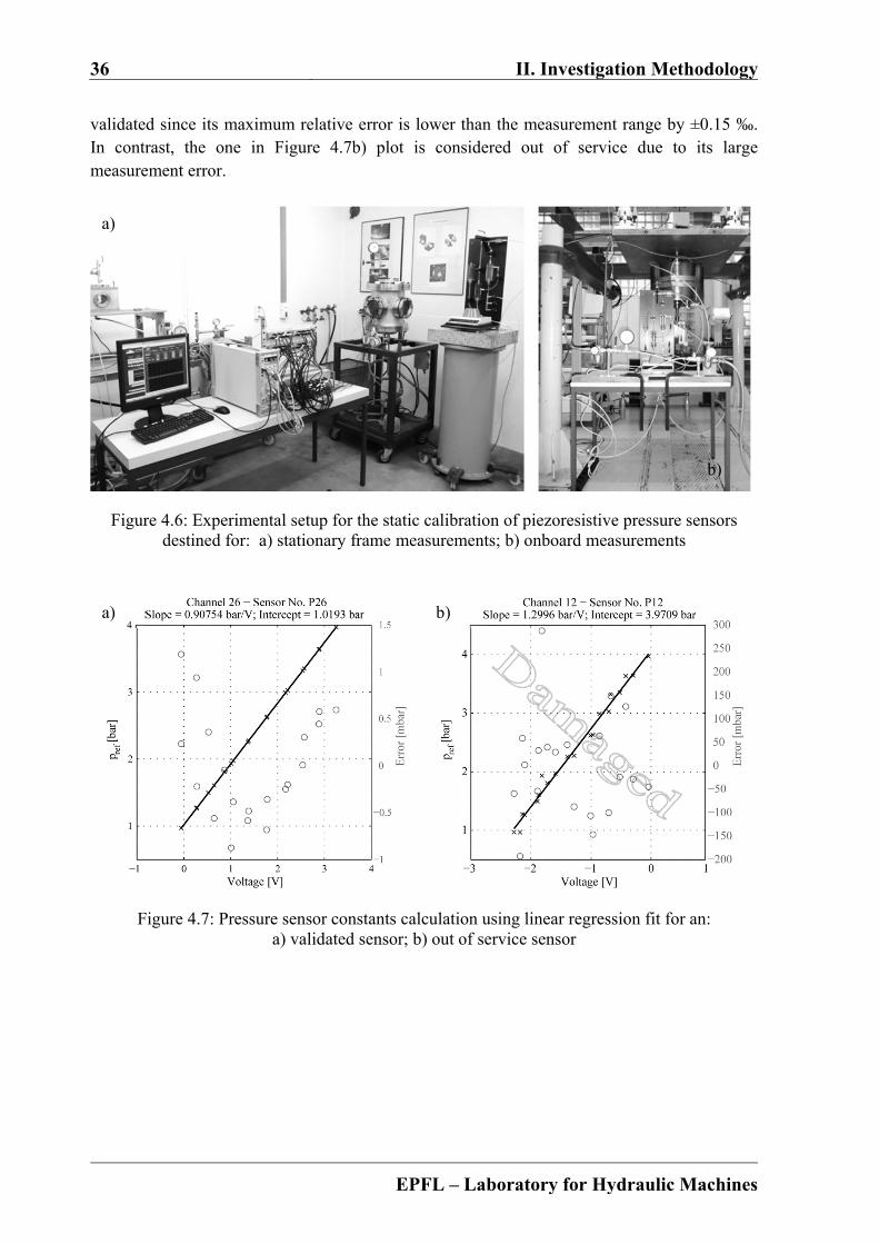
36 II. Investigation Methodology
EPFL – Laboratory for Hydraulic Machines
validated since its maximum relative error is lower than the measurement range by ±0.15 ‰. In contrast, the one in Figure 4.7b) plot is considered out of service due to its large measurement error.
Figure 4.6: Experimental setup for the static calibration of piezoresistive pressure sensors destined for: a) stationary frame measurements; b) onboard measurements
Figure 4.7: Pressure sensor constants calculation using linear regression fit for an: a) validated sensor; b) out of service sensor
a)
b)
a) b)
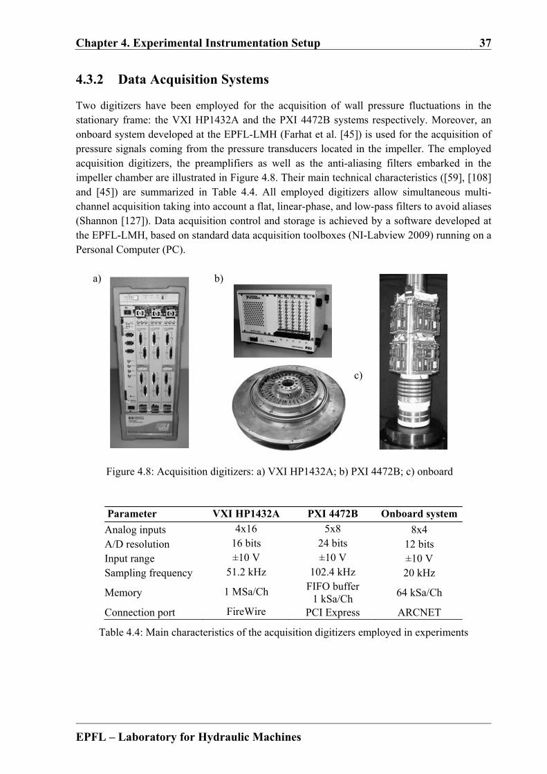
Chapter 4. Experimental Instrumentation Setup 37
EPFL – Laboratory for Hydraulic Machines
4.3.2 Data Acquisition Systems
Two digitizers have been employed for the acquisition of wall pressure fluctuations in the stationary frame: the VXI HP1432A and the PXI 4472B systems respectively. Moreover, an onboard system developed at the EPFL-LMH (Farhat et al. [45]) is used for the acquisition of pressure signals coming from the pressure transducers located in the impeller. The employed acquisition digitizers, the preamplifiers as well as the anti-aliasing filters embarked in the impeller chamber are illustrated in Figure 4.8. Their main technical characteristics ([59], [108] and [45]) are summarized in Table 4.4. All employed digitizers allow simultaneous multi-channel acquisition taking into account a flat, linear-phase, and low-pass filters to avoid aliases (Shannon [127]). Data acquisition control and storage is achieved by a software developed at the EPFL-LMH, based on standard data acquisition toolboxes (NI-Labview 2009) running on a Personal Computer (PC).
a)
b)
c)
Figure 4.8: Acquisition digitizers: a) VXI HP1432A; b) PXI 4472B; c) onboard
Parameter VXI HP1432A PXI 4472B Onboard system
Analog inputs 4x16 5x8 8x4 A/D resolution 16 bits 24 bits 12 bits Input range ±10 V ±10 V ±10 V Sampling frequency 51.2 kHz 102.4 kHz 20 kHz
Memory 1 MSa/Ch FIFO buffer 1 kSa/Ch
64 kSa/Ch
Connection port FireWire PCI Express ARCNET
Table 4.4: Main characteristics of the acquisition digitizers employed in experiments
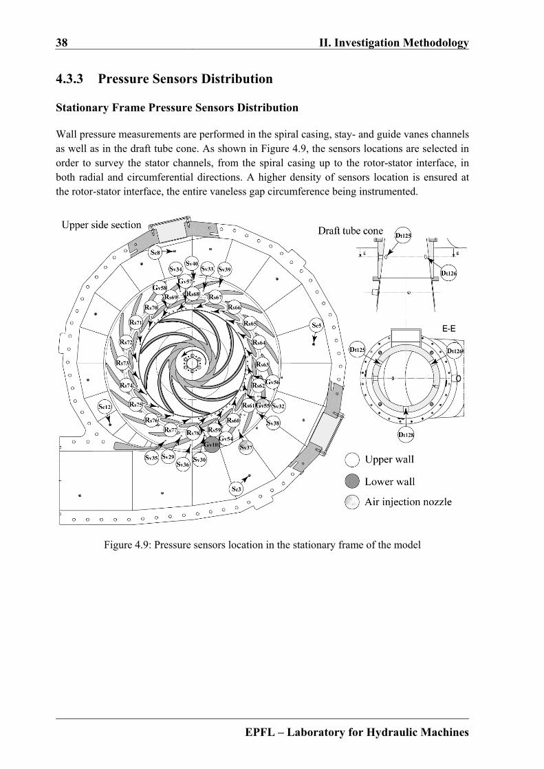
38 II. Investigation Methodology
EPFL – Laboratory for Hydraulic Machines
4.3.3 Pressure Sensors Distribution
Stationary Frame Pressure Sensors Distribution
Wall pressure measurements are performed in the spiral casing, stay- and guide vanes channels as well as in the draft tube cone. As shown in Figure 4.9, the sensors locations are selected in order to survey the stator channels, from the spiral casing up to the rotor-stator interface, in both radial and circumferential directions. A higher density of sensors location is ensured at the rotor-stator interface, the entire vaneless gap circumference being instrumented.
Figure 4.9: Pressure sensors location in the stationary frame of the model
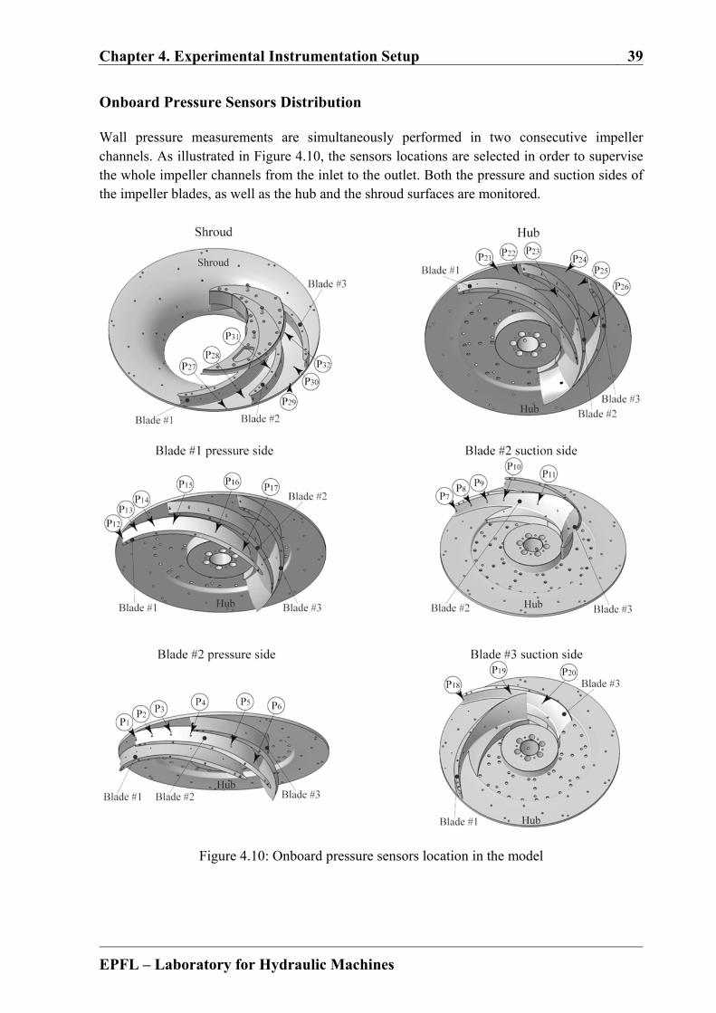
Chapter 4. Experimental Instrumentation Setup 39
EPFL – Laboratory for Hydraulic Machines
Onboard Pressure Sensors Distribution
Wall pressure measurements are simultaneously performed in two consecutive impeller channels. As illustrated in Figure 4.10, the sensors locations are selected in order to supervise the whole impeller channels from the inlet to the outlet. Both the pressure and suction sides of the impeller blades, as well as the hub and the shroud surfaces are monitored.
Figure 4.10: Onboard pressure sensors location in the model

40 II. Investigation Methodology
EPFL – Laboratory for Hydraulic Machines
4.4 Particle Image Velocimetry
Measurement Principle of PIV
Particle Image Velocimetry (PIV) is a non-intrusive measurement technique of the instantaneous velocity vectors in a cross-section of a flow. The working principle of PIV is illustrated in Figure 4.11. The measurement is based on the analysis of two successive images of the target area seeded with micro-sized particles that follow the flow and that are illuminated with a laser sheet provided by a double-pulsed laser. Consequently, the images captured with a CCD camera are divided into rectangular regions called interrogation areas. As a subsequent step, the interrogation areas of each image frame - I1 and I2 - are cross-correlated with each other, pixel by pixel, in order to produce an average particle displacement vector. Equation (4.5) includes the spatial cross-correlation function of separation vector s - as defined in Keane and Adrian [79] - for an interrogation area between the two frames.
1 2 1 2I I IA
C s I X I X s dX (4.5)
A signal peak provided by the correlation is used to identify the particle displacement. Moreover, it is possible to achieve an accurate measure of the displacement, and implicitly, of the velocity, if a sub-pixel interpolation is employed. By repeating the cross-correlation for each interrogation area of the two image frames that are captured by the camera, it is possible to obtain a velocity vector map of the whole target area.
Figure 4.11: Working principle of Particle Image Velocimetry (PIV), [31]
PIV Measurements Setup
In recent years, there has been an increasing interest in using the PIV technique to investigate the onset, the development of flow separation (Pedersen et al. [114]) and stall phenomena in turbomachines. Hence, several experimental investigations of rotating stall developed in the stator (Sinha et al. [131], Miyabe et al. [106] and Dazin et al. [33]) or in the impeller (Krause
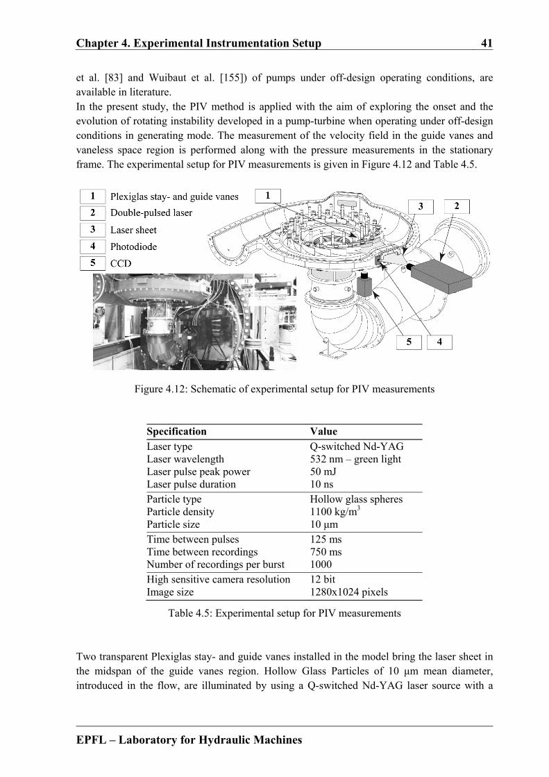
Chapter 4. Experimental Instrumentation Setup 41
EPFL – Laboratory for Hydraulic Machines
et al. [83] and Wuibaut et al. [155]) of pumps under off-design operating conditions, are available in literature. In the present study, the PIV method is applied with the aim of exploring the onset and the evolution of rotating instability developed in a pump-turbine when operating under off-design conditions in generating mode. The measurement of the velocity field in the guide vanes and vaneless space region is performed along with the pressure measurements in the stationary frame. The experimental setup for PIV measurements is given in Figure 4.12 and Table 4.5.
Figure 4.12: Schematic of experimental setup for PIV measurements
Specification Value
Laser type Q-switched Nd-YAG Laser wavelength 532 nm – green light Laser pulse peak power 50 mJ Laser pulse duration 10 ns Particle type Hollow glass spheres Particle density 1100 kg/m3 Particle size 10 μm Time between pulses 125 ms Time between recordings 750 ms Number of recordings per burst 1000 High sensitive camera resolution 12 bit Image size 1280x1024 pixels
Table 4.5: Experimental setup for PIV measurements Two transparent Plexiglas stay- and guide vanes installed in the model bring the laser sheet in the midspan of the guide vanes region. Hollow Glass Particles of 10 μm mean diameter, introduced in the flow, are illuminated by using a Q-switched Nd-YAG laser source with a
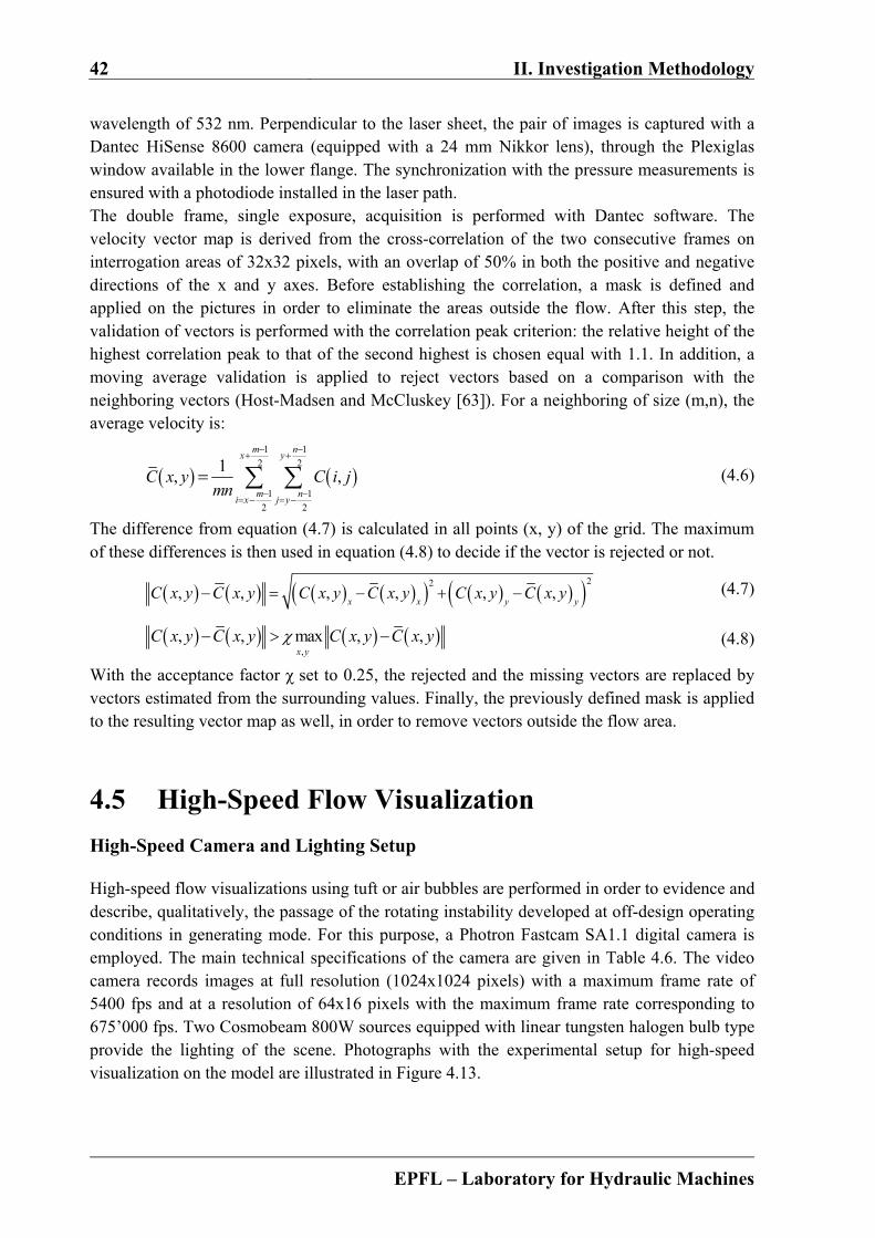
42 II. Investigation Methodology
EPFL – Laboratory for Hydraulic Machines
wavelength of 532 nm. Perpendicular to the laser sheet, the pair of images is captured with a Dantec HiSense 8600 camera (equipped with a 24 mm Nikkor lens), through the Plexiglas window available in the lower flange. The synchronization with the pressure measurements is ensured with a photodiode installed in the laser path. The double frame, single exposure, acquisition is performed with Dantec software. The velocity vector map is derived from the cross-correlation of the two consecutive frames on interrogation areas of 32x32 pixels, with an overlap of 50% in both the positive and negative directions of the x and y axes. Before establishing the correlation, a mask is defined and applied on the pictures in order to eliminate the areas outside the flow. After this step, the validation of vectors is performed with the correlation peak criterion: the relative height of the highest correlation peak to that of the second highest is chosen equal with 1.1. In addition, a moving average validation is applied to reject vectors based on a comparison with the neighboring vectors (Host-Madsen and McCluskey [63]). For a neighboring of size (m,n), the average velocity is:
1 1
2 2
1 1
2 2
1, ,
m nx y
m ni x j y
C x y C i jmn
(4.6)
The difference from equation (4.7) is calculated in all points (x, y) of the grid. The maximum of these differences is then used in equation (4.8) to decide if the vector is rejected or not.
22, , , , , ,
x x y yC x y C x y C x y C x y C x y C x y (4.7)
,
, , max , ,x y
C x y C x y C x y C x y (4.8)
With the acceptance factor χ set to 0.25, the rejected and the missing vectors are replaced by vectors estimated from the surrounding values. Finally, the previously defined mask is applied to the resulting vector map as well, in order to remove vectors outside the flow area.
4.5 High-Speed Flow Visualization
High-Speed Camera and Lighting Setup
High-speed flow visualizations using tuft or air bubbles are performed in order to evidence and describe, qualitatively, the passage of the rotating instability developed at off-design operating conditions in generating mode. For this purpose, a Photron Fastcam SA1.1 digital camera is employed. The main technical specifications of the camera are given in Table 4.6. The video camera records images at full resolution (1024x1024 pixels) with a maximum frame rate of 5400 fps and at a resolution of 64x16 pixels with the maximum frame rate corresponding to 675’000 fps. Two Cosmobeam 800W sources equipped with linear tungsten halogen bulb type provide the lighting of the scene. Photographs with the experimental setup for high-speed visualization on the model are illustrated in Figure 4.13.
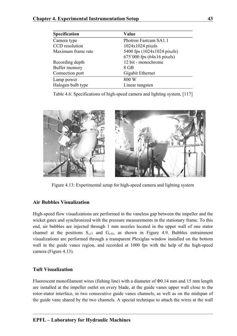
Chapter 4. Experimental Instrumentation Setup 43
EPFL – Laboratory for Hydraulic Machines
Specification Value Camera type Photron Fastcam SA1.1 CCD resolution 1024x1024 pixels Maximum frame rate 5400 fps (1024x1024 pixels)
675`000 fps (64x16 pixels) Recording depth 12 bit - monochrome Buffer memory 8 GB Connection port Gigabit Ethernet Lamp power 800 W Halogen bulb type Linear tungsten
Table 4.6: Specifications of high-speed camera and lighting system, [117]
Figure 4.13: Experimental setup for high-speed camera and lighting system
Air Bubbles Visualization
High-speed flow visualizations are performed in the vaneless gap between the impeller and the wicket gates and synchronized with the pressure measurements in the stationary frame. To this end, air bubbles are injected through 1 mm nozzles located in the upper wall of one stator channel at the positions Sv37 and Gv55, as shown in Figure 4.9. Bubbles entrainment visualizations are performed through a transparent Plexiglas window installed on the bottom wall in the guide vanes region, and recorded at 1000 fps with the help of the high-speed camera (Figure 4.13).
Tuft Visualization
Fluorescent monofilament wires (fishing line) with a diameter of Φ0.14 mm and 15 mm length are installed at the impeller outlet on every blade, at the guide vanes upper wall close to the rotor-stator interface, in two consecutive guide vanes channels, as well as on the midspan of the guide vane shared by the two channels. A special technique to attach the wires at the wall
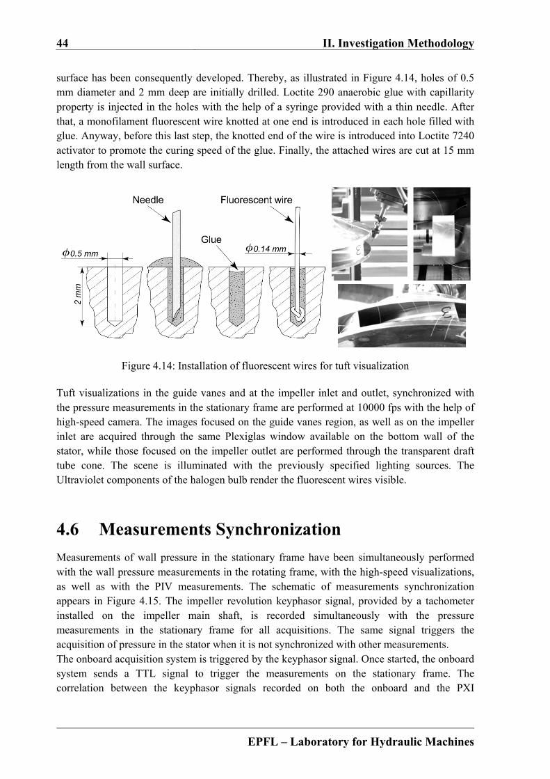
44 II. Investigation Methodology
EPFL – Laboratory for Hydraulic Machines
surface has been consequently developed. Thereby, as illustrated in Figure 4.14, holes of 0.5 mm diameter and 2 mm deep are initially drilled. Loctite 290 anaerobic glue with capillarity property is injected in the holes with the help of a syringe provided with a thin needle. After that, a monofilament fluorescent wire knotted at one end is introduced in each hole filled with glue. Anyway, before this last step, the knotted end of the wire is introduced into Loctite 7240 activator to promote the curing speed of the glue. Finally, the attached wires are cut at 15 mm length from the wall surface.
Figure 4.14: Installation of fluorescent wires for tuft visualization Tuft visualizations in the guide vanes and at the impeller inlet and outlet, synchronized with the pressure measurements in the stationary frame are performed at 10000 fps with the help of high-speed camera. The images focused on the guide vanes region, as well as on the impeller inlet are acquired through the same Plexiglas window available on the bottom wall of the stator, while those focused on the impeller outlet are performed through the transparent draft tube cone. The scene is illuminated with the previously specified lighting sources. The Ultraviolet components of the halogen bulb render the fluorescent wires visible.
4.6 Measurements Synchronization
Measurements of wall pressure in the stationary frame have been simultaneously performed with the wall pressure measurements in the rotating frame, with the high-speed visualizations, as well as with the PIV measurements. The schematic of measurements synchronization appears in Figure 4.15. The impeller revolution keyphasor signal, provided by a tachometer installed on the impeller main shaft, is recorded simultaneously with the pressure measurements in the stationary frame for all acquisitions. The same signal triggers the acquisition of pressure in the stator when it is not synchronized with other measurements. The onboard acquisition system is triggered by the keyphasor signal. Once started, the onboard system sends a TTL signal to trigger the measurements on the stationary frame. The correlation between the keyphasor signals recorded on both the onboard and the PXI

Chapter 4. Experimental Instrumentation Setup 45
EPFL – Laboratory for Hydraulic Machines
acquisition systems is then used to recheck the synchronization during the merge of the two initially stored independent measurement files into a common hdf-5 file. The synchronization between the PIV and the pressure measurements is ensured by the presence of a photodiode installed in the laser path. Indeed, the first laser pulse triggers the pressure measurements in the stator. However, the signal generated by the photodiode is acquired simultaneously with the pressure during all the 1000 PIV recordings per burst. In the case of high-speed flow visualizations, the pressure measurements in the stationary frame are triggered by a TTL signal sent from the high-speed camera once a new recording is started.
Figure 4.15: Schematic of measurements synchronization


EPFL – Laboratory for Hydraulic Machines
Chapter 5
Numerical Modeling
Experimental investigations of flow hydrodynamics even in reduced scale model of hydraulic turbomachines are sometimes technically limited or too expensive in terms of time and costs. Therefore, numerical simulations can be a relatively fast and cost effective mean to evaluate performances and to explore the flow hydrodynamics. Because the fact that there are limitations on the models implemented in the numerical simulations, special cases need to be validated by experimental measurements (Hasmatuchi et al. [54]). In spite of the fact that a large volume of numerical studies have already been conducted on the hydrodynamics of hydraulic turbomachines, the operation of pump-turbines under off-design conditions in generating mode remains poorly addressed in literature.
5.1 Governing Equations
Incompressible Navier-Stokes Equation
Fluid flow results from the action of externally applied forces such as the pressure, the shear forces produced by the motion of a solid surface relative to the fluid (surface forces), the gravity, and the rotation-induced forces (body forces), Ferziger and Peric [47]. More precisely, the fluid motion is governed by the mass and momentum conservation laws, also known as Navier-Stokes equations. In the case of an incompressible fluid with constant density, the time-dependent form of these nonlinear partial differential equations in space and time - in a Cartesian coordinates system - may be expressed in the following way:
0i
i
C
x
(5.1)
1 iji ij i
j i j
C C pC f
t x x x
(5.2)
According to the continuity equation (5.1) applied to a control volume, the fluid mass does not vary in time. The conservation law of momentum (5.2) is derived from the Newton’s second law of motion which states that the rate of change in momentum of the body is directly
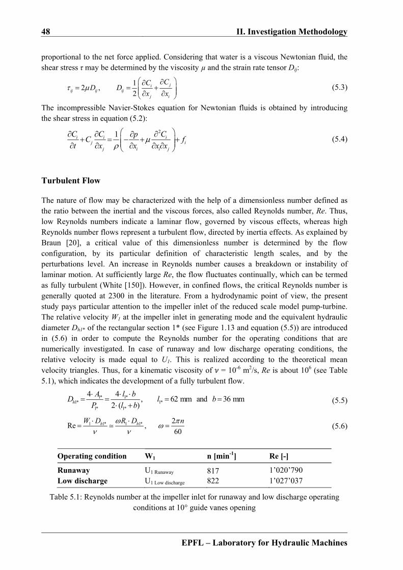
48 II. Investigation Methodology
EPFL – Laboratory for Hydraulic Machines
proportional to the net force applied. Considering that water is a viscous Newtonian fluid, the shear stress τ may be determined by the viscosity µ and the strain rate tensor Dij:
12 ,
2ji
ij ij ijj i
CCD D
x x
(5.3)
The incompressible Navier-Stokes equation for Newtonian fluids is obtained by introducing the shear stress in equation (5.2):
21i i ij i
j i i j
C C CpC f
t x x x x
(5.4)
Turbulent Flow
The nature of flow may be characterized with the help of a dimensionless number defined as the ratio between the inertial and the viscous forces, also called Reynolds number, Re. Thus, low Reynolds numbers indicate a laminar flow, governed by viscous effects, whereas high Reynolds number flows represent a turbulent flow, directed by inertia effects. As explained by Braun [20], a critical value of this dimensionless number is determined by the flow configuration, by its particular definition of characteristic length scales, and by the perturbations level. An increase in Reynolds number causes a breakdown or instability of laminar motion. At sufficiently large Re, the flow fluctuates continually, which can be termed as fully turbulent (White [150]). However, in confined flows, the critical Reynolds number is generally quoted at 2300 in the literature. From a hydrodynamic point of view, the present study pays particular attention to the impeller inlet of the reduced scale model pump-turbine. The relative velocity W1 at the impeller inlet in generating mode and the equivalent hydraulic diameter Dh1* of the rectangular section 1* (see Figure 1.13 and equation (5.5)) are introduced in (5.6) in order to compute the Reynolds number for the operating conditions that are numerically investigated. In case of runaway and low discharge operating conditions, the relative velocity is made equal to U1. This is realized according to the theoretical mean velocity triangles. Thus, for a kinematic viscosity of = 10-6 m2/s, Re is about 106 (see Table 5.1), which indicates the development of a fully turbulent flow.
1* 1*1* 1*
1* 1*
4 4, 62 mm and 36 mm
2 ( )h
A l bD l b
P l b
(5.5)
1 1* 1 1* 2Re ,
60h hW D R D n
(5.6)
Operating condition W1 n [min-1] Re [-]
Runaway U1 Runaway 817 1’020’790 Low discharge U1 Low discharge 822 1’027’037
Table 5.1: Reynolds number at the impeller inlet for runaway and low discharge operating conditions at 10° guide vanes opening
Chapter 5. Numerical Modeling 49
EPFL – Laboratory for Hydraulic Machines
Reynolds-Averaged Navier-Stokes Equations
In the case of inviscid or laminar flow, the solution of Navier-Stokes equations may be obtained analytically. Instead, the simulation of turbulent flows represents a real challenge. Despite the performance of modern supercomputers, a direct numerical simulation (DNS) of turbulence by the time-dependent Navier-Stokes equations remains suitable only for rather simple flow cases at low Reynolds numbers. The restrictions of the DNS comes from the fact that the number of grid points needed for sufficient spatial resolution scales as Re9/4, whereas the time resolution as Re3/4, which leads to a CPU-time scaling as Re3 (Sagaut [124], Blazek [15]). Therefore, when the flow is turbulent, it is preferable to separate any instantaneous scalar variable (e.g. velocity components and pressure) into a mean and a fluctuating value (Davidson [32]):
'( , ) ( , ) ( , )i i i i i iC x t C x t C x t (5.7)
In the Reynolds-averaged approach, the mean value is associated with a time-average - for a steady flow - or with a set of averaging, in the case of a time-dependent mean flow.
Considering that the mean value is not time-dependent and that the mean value of a
fluctuating part is zero ′ 0, the continuity and momentum equations become:
'
0i
i
C
x
(5.8)
' '2
2
1 i ji i ij i
j i j j
CCC C CpC f
t x x x x
(5.9)
In the incompressible Reynolds-Averaged Navier-Stokes (RANS) equations, the Reynolds
stresses term , with 6 new unknowns, is the only accountable difference to the Navier-
Stokes equations. The new system formed by the conservation equations is not closed since the number of variables is larger than the number of equations. It becomes therefore necessary to make assumptions (turbulence models) in order to predict the Reynolds stresses and to close the system.
5.2 Turbulence Modeling
Flow separation is an extremely complex problem for CFD. Indeed, the CFD code has to be able to model the unsteadiness of separated flow, the high turbulent flow regions and the boundary layer effects. The most efficient way to capture these effects would be a Direct Numerical Simulation (DNS), the reason being that it solves exactly the Navier-Stokes equations. However, as claimed by Hirsch and Tartinville [60], the DNS requires a very fine mesh and too much computational resources for common industrial problems. In order to solve the Navier-Stokes equations for such complicated problems, not only must CFD users make some assumptions but they also have to apply turbulence modeling (Corson et al. [29]). A typical approach is the Reynolds-Averaged Navier-Stokes, which consists in splitting each

50 II. Investigation Methodology
EPFL – Laboratory for Hydraulic Machines
variable of the Navier-Stokes equations into a mean and a fluctuating component (Ryhming [123]). This difficulty of capturing the turbulence and its effect in a satisfying way has led to the development of several different turbulence models. Many recommendations about these models are given in the literature, for instance in Zingg & Godin [157] or in Batten et al. [10]. Although some common turbulent models are in good agreement with experimental studies, they all present several deficiencies (Hirsch and Tartinville [60]). Indeed, Zingg and Godin [157] mention that each turbulence model can be tuned to reach a specific known result. The first approach to turbulence modeling consists in replacing the Reynolds stresses term from the RANS equation with an eddy viscosity equation, (5.10). The most famous modeling used for common industrial problems is the k-ε turbulence model. This model expresses the turbulent eddy viscosity µT as a function of the turbulent kinetic energy of flow k and its rate of dissipation ε, (5.11). However, Menter [102] notices the limitations of the k-ε turbulence model in the near wall areas or in predicting flow separation.
' 'i j ji
Tj j i
CC CC
x x x
(5.10)
2
, 0.09T
kC C
(5.11)
Therefore, an alternative is the k-ω turbulence model, which is more accurate in the boundary layers. This model expresses the turbulent eddy viscosity µT as a function of the turbulent kinetic energy of the flow k and the turbulent frequency ω:
, with , - turbulence length scaleT tt
k kL
C L
(5.12)
Nevertheless, since this model is less accurate than the k-ε model in the free stream outside of the boundary layer area (Menter et al. [103]), the Shear Stress Transport (SST) turbulence model is considered to be even better than the two just mentioned, the reason being that it finds the most appropriate turbulence model between k-ε and k-ω for each location in the computational domain. As described by Menter et al. [103], the splitting of the computational domain is done by a blending function, which computes the distance from wall by using the solution of a Poisson equation and chooses the most appropriate turbulence model. Notwithstanding, it was found (Braza et al. [21], Launder [88]) that eddy viscosity models do not capture correctly the flow unsteadiness and the body forces. Consequently, the results show inaccurate reattachment and poor treatment of massive separation, in both steady and unsteady (URANS) calculations, Spalart [135]. Rumsey and Swanson [122] discuss the incapability of RANS methods to predict steady and unsteady active flow control cases with accuracy and confidence. The Large Eddy Simulation (LES) is trade-off between DNS and RANS approaches. Actually, LES does not use the RANS formulation but applies a grid filter on the standard Navier-Stokes equations and provide, with a high precision, the fluctuation values of velocity and pressure (Lesieur [91]). This filter allows splitting the length scales present in the flow in two categories: solved or modeled. Since the solved length scales are bigger than the length scale

Chapter 5. Numerical Modeling 51
EPFL – Laboratory for Hydraulic Machines
represented by the mesh, they are solved as DNS. Moreover, Sagaut [124] argues that the modeled length scales need to be modeled because they cannot be taken into account by the mesh. Usually, the LES turbulence model allows a better physical representation than the RANS formulation. However, for confined flow, a thinner mesh refinement and a very good knowledge of the inlet boundary condition are required if researchers want to obtain a more accurate result (Kaltenbach et al. [77]). It should be clarified that Detached Eddy Simulation (DES) is a hybrid turbulence model that attempts to combine the best aspects of the LES and RANS methodologies. This model treats the near-wall region with RANS and the rest of the flow with LES. Byskov et al. [23] found that LES combined with eddy viscosity subgrid-scale models approach shows considerable accuracy in simulating a centrifugal pump dominated by flow separation. Scale Adaptive Simulation (SAS) is a method similar to DES that adapts the turbulence model in function of the turbulence length scale, by using a RANS model in the steady flow regions and a LES one in the unsteady ones. If SAS is essentially an improved URANS formulation that allows the resolution of the turbulent spectrum in unstable flow conditions, DES is a combination of RANS and LES methods. The switch between the two is achieved by comparing of the modeled turbulent length scale and the grid spacing. As the grid spacing explicitly enters the DES equations, DES has significantly stronger mesh sensitivity than SAS. The main practical problems with DES are that certain requirements have to be satisfied in the switching zone between RANS and LES (Spalart [134]). The model employed in this study, summarized in Egorov and Menter [42], dynamically adjusts the turbulence scale equation with the help of the von Karman length scale LvK (equation (5.13)). Based on the second derivatives of the velocity C’’ (equation (5.14)), the term varies with the level of the local flow inhomogeneities.
2
''max , , withvK S
kkSL C
CC
(5.13)
1 32 , , 0.41 - von Karman constantij ijS D D k (5.14)
22
''
( )
i
i j j
CC
x x
(5.15)
This lower limiter applied to the von Karman length scale is proportional to the cubic root of the control volume size Ω. Indeed, it controls the damping of the finest resolved turbulent fluctuations allowing the break-up of large unsteady structures into a turbulent spectrum, Meter and Egorov [104]. The structure of the limiter is derived from the equilibrium of the eddy viscosity of the SST-SAS model. The balance between production and destruction of the kinetic energy of turbulence leads to the following relation for the equilibrium viscosity:
2
2 2/ , 3.51, 5 9, 3 40eqt vKC k L S (5.16)
This expression is similar to the subgrid scale eddy viscosity in the Smagorinsky LES model:
2LESt SC S (5.17)
52 II. Investigation Methodology
EPFL – Laboratory for Hydraulic Machines
Consequently, the limiter imposed on the von Karman length scale value must avoid that SAS eddy viscosity decreases and goes below the LES subgrid scale eddy viscosity: µt
eq ≥ µtLES. The
model parameter CS = 0.11, calibrated through the employment of decaying isotropic turbulence, ensures a similar energy spectrum as the one obtained with the Smagorinsky LES model. When dealing with strongly unstable flows, Egorov et al. [41] assert that the SAS model offers an attractive alternative to the existing “hybrid” RANS/LES methods. Moreover, the potential of SAS models in simulating engineering flows is demonstrated by several test cases in Menter and Egorov [105]. However, a drawback of this turbulence model would be the total simulation time that must be long enough to let the turbulence develop, Younsi et al. [156].
5.3 Numerical Scheme
The numerical scheme applied to the simulation of the flow in the full reduced scale model water passage from the spiral casing inlet to the draft tube outlet is summarized in Table 5.2. The Ansys CFX 12 commercial code [4] is used in order to perform unsteady incompressible turbulent flow numerical simulation, while the finite volume method is employed in order to solve both the incompressible Unsteady Reynolds-Averaged Navier-Stokes (URANS) equations in their conservative form and the mass conservation equations. The set of equations is closed in a two-equation turbulence model. The hybrid RANS-LES turbulence model based on the von Karman length scale for blending function, called SAS-SST is employed. The reason why this turbulence model has been selected lies in the fact that the SAS-SST captures the qualitative aspects of flow separation phenomenon well. Furthermore, it must be clarified that this model constitutes a good compromise between the computational time and costs on the one hand, and the results accuracy on the other hand. An advection scheme (2nd order in space) and the backward Euler implicit scheme (2nd order in time) are used. Finally, a time step corresponding to 1° of impeller revolution and a convergence criterion RMSmax < 10-3 with 10 internal coefficient loops are selected.
Simulation type Unsteady Turbulence model SAS-SST Computational domain Full reduced scale model Time step 1° of impeller revolution Convergence criterion RMSMAX < 10-3 - 10 internal coefficient loops Simulation duration > 30 impeller revolutions
Table 5.2: Numerical scheme
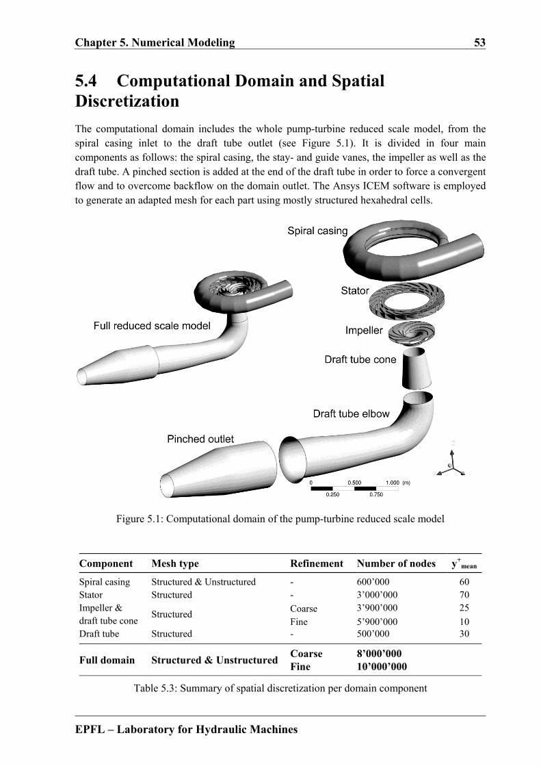
Chapter 5. Numerical Modeling 53
EPFL – Laboratory for Hydraulic Machines
5.4 Computational Domain and Spatial Discretization
The computational domain includes the whole pump-turbine reduced scale model, from the spiral casing inlet to the draft tube outlet (see Figure 5.1). It is divided in four main components as follows: the spiral casing, the stay- and guide vanes, the impeller as well as the draft tube. A pinched section is added at the end of the draft tube in order to force a convergent flow and to overcome backflow on the domain outlet. The Ansys ICEM software is employed to generate an adapted mesh for each part using mostly structured hexahedral cells.
Figure 5.1: Computational domain of the pump-turbine reduced scale model
Component Mesh type Refinement Number of nodes y+mean
Spiral casing Structured & Unstructured - 600’000 60 Stator Structured - 3’000’000 70 Impeller & draft tube cone
Structured Coarse 3’900’000 25
Fine 5’900’000 10 Draft tube Structured - 500’000 30
Full domain Structured & Unstructured Coarse 8’000’000 Fine 10’000’000
Table 5.3: Summary of spatial discretization per domain component
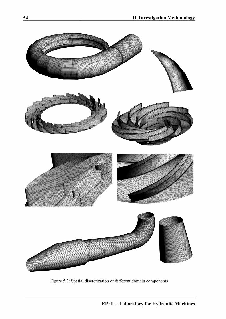
54 II. Investigation Methodology
EPFL – Laboratory for Hydraulic Machines
Figure 5.2: Spatial discretization of different domain components

Chapter 5. Numerical Modeling 55
EPFL – Laboratory for Hydraulic Machines
Anyway, for the spiral casing tongue, an unstructured mesh with tetrahedral cells is generated (Figure 5.2). This is due to the sharp end of the tongue. A distribution law is used in the mesh generation close to every solid surface in order to ensure an appropriate modeling of the boundary layer. The number of nodes for each domain component is summarized in Table 5.3 along with the average dimensionless wall distance y+
mean. One may be observed that a larger density of nodes is ensured in the stay- and guide vanes region, as well as in the impeller, where more than 50% of the total number of nodes is allocated.
**
*
Cy
yy
(5.18)
The dimensionless normal distance to the wall y+, which depends on the distance to the nearest wall y*, the friction velocity at the nearest wall C* and the kinematic viscosity υ (equation (5.18)), is also lower in the impeller region than in the other components. The reason for such a mesh density distribution is the location that the flow instabilities development takes when the machine is operated under off-design conditions in generating mode.
Spatial discretization refinement
Two different mesh refinements for the impeller region are employed, a coarse and a fine one (Figure 5.3) respectively. The influence of the mesh refinement on the numerical simulation of flow at low discharge operating condition can be observed in Figure 5.4. Thus, the contour of dimensionless vorticity around the z axis ωz
* on the impeller midspan (equation (5.19)) shows the way the flow separation is artificially vanished close to the impeller inlet in the case of coarse mesh, whilst using a refined mesh the flow separation is extended into the whole impeller channels.
* 1
2y x
zn
C C
x y f
(5.19)
Figure 5.3: Mesh refinement in the impeller: a) coarse; b) fine
a) b)
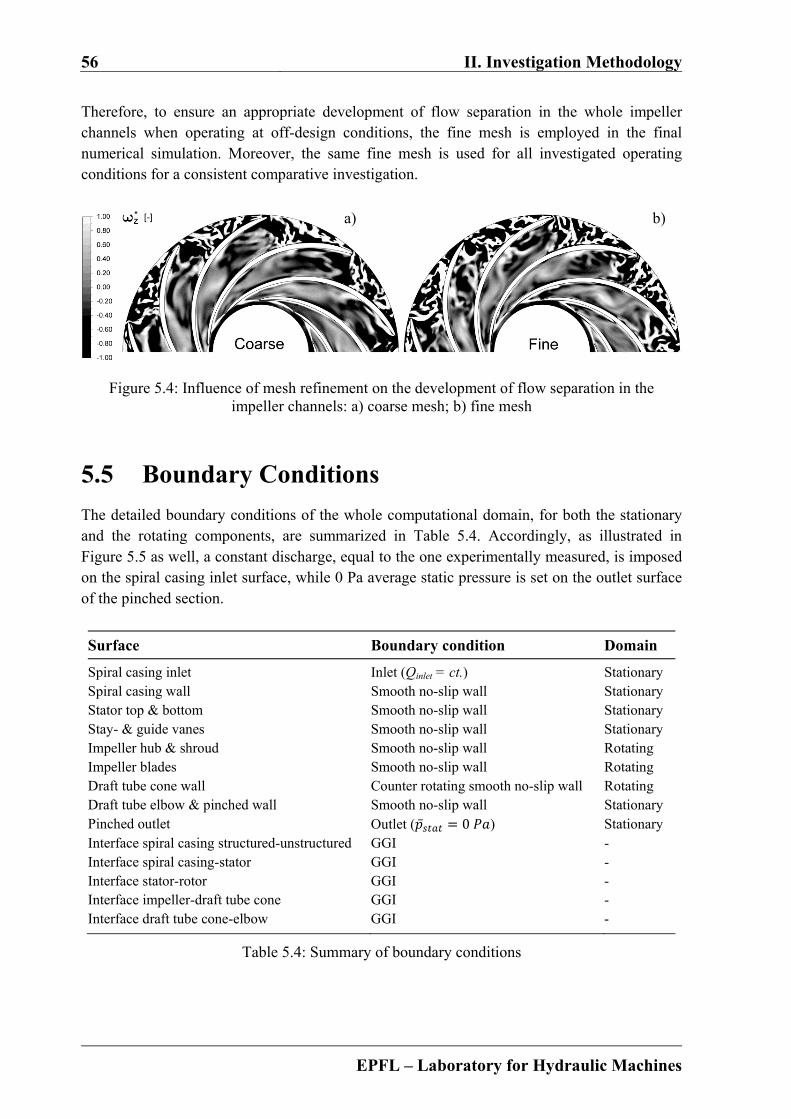
56 II. Investigation Methodology
EPFL – Laboratory for Hydraulic Machines
Therefore, to ensure an appropriate development of flow separation in the whole impeller channels when operating at off-design conditions, the fine mesh is employed in the final numerical simulation. Moreover, the same fine mesh is used for all investigated operating conditions for a consistent comparative investigation.
Figure 5.4: Influence of mesh refinement on the development of flow separation in the impeller channels: a) coarse mesh; b) fine mesh
5.5 Boundary Conditions
The detailed boundary conditions of the whole computational domain, for both the stationary and the rotating components, are summarized in Table 5.4. Accordingly, as illustrated in Figure 5.5 as well, a constant discharge, equal to the one experimentally measured, is imposed on the spiral casing inlet surface, while 0 Pa average static pressure is set on the outlet surface of the pinched section.
Surface Boundary condition Domain
Spiral casing inlet Inlet (Qinlet = ct.) Stationary Spiral casing wall Smooth no-slip wall Stationary Stator top & bottom Smooth no-slip wall Stationary Stay- & guide vanes Smooth no-slip wall Stationary Impeller hub & shroud Smooth no-slip wall Rotating Impeller blades Smooth no-slip wall Rotating Draft tube cone wall Counter rotating smooth no-slip wall Rotating Draft tube elbow & pinched wall Smooth no-slip wall Stationary Pinched outlet Outlet ( 0 ) Stationary Interface spiral casing structured-unstructured GGI - Interface spiral casing-stator GGI - Interface stator-rotor GGI - Interface impeller-draft tube cone GGI - Interface draft tube cone-elbow GGI -
Table 5.4: Summary of boundary conditions
a) b)
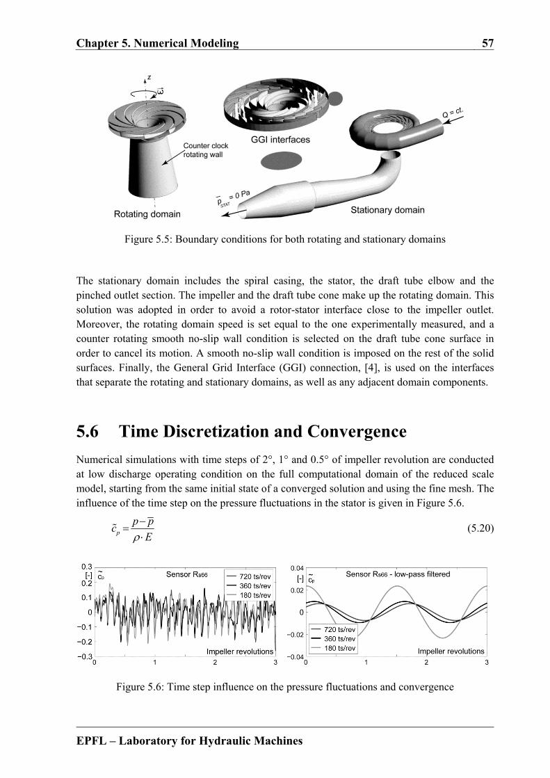
Chapter 5. Numerical Modeling 57
EPFL – Laboratory for Hydraulic Machines
Figure 5.5: Boundary conditions for both rotating and stationary domains The stationary domain includes the spiral casing, the stator, the draft tube elbow and the pinched outlet section. The impeller and the draft tube cone make up the rotating domain. This solution was adopted in order to avoid a rotor-stator interface close to the impeller outlet. Moreover, the rotating domain speed is set equal to the one experimentally measured, and a counter rotating smooth no-slip wall condition is selected on the draft tube cone surface in order to cancel its motion. A smooth no-slip wall condition is imposed on the rest of the solid surfaces. Finally, the General Grid Interface (GGI) connection, [4], is used on the interfaces that separate the rotating and stationary domains, as well as any adjacent domain components.
5.6 Time Discretization and Convergence
Numerical simulations with time steps of 2°, 1° and 0.5° of impeller revolution are conducted at low discharge operating condition on the full computational domain of the reduced scale model, starting from the same initial state of a converged solution and using the fine mesh. The influence of the time step on the pressure fluctuations in the stator is given in Figure 5.6.
p
p pc
E
(5.20)
Figure 5.6: Time step influence on the pressure fluctuations and convergence

58 II. Investigation Methodology
EPFL – Laboratory for Hydraulic Machines
On the one hand, the amplitude and frequency of pressure coefficient fluctuation (equation (5.20)), in the vaneless gap between the impeller and guide vanes (pressure sensor location RS66), caused by the rotor-stator interaction (9·fn and its harmonics 18·fn, 27·fn, …) reveals no significant differences between the three tested time steps. On the other hand, when using a time step of 2°, the amplitude shown by the pressure fluctuations related to the development of the rotating-stall (~0.7·fn) and represented with the help of the low-pass filtered pressure coefficient, is larger than the one that emerges when using a time step of 1° and 0.5° of impeller revolution. However, no significant difference is obtained between the time steps of 1° and 0.5°. Therefore, as justified also by Braun [20], who modeled numerically a rotating stall in pumping mode for the same pump-turbine scale model, the time step of 1° is found to be an appropriate compromise between solution accuracy and computational costs even in off-design conditions.
Figure 5.7: Spatial discretization influence on the pressure fluctuations and convergence for normal operating range condition
Figure 5.8: Time step influence on the convergence for low discharge operating condition
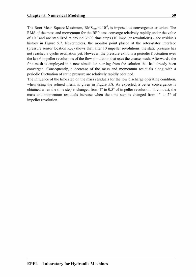
Chapter 5. Numerical Modeling 59
EPFL – Laboratory for Hydraulic Machines
The Root Mean Square Maximum, RMSmax < 10-3, is imposed as convergence criterion. The RMS of the mass and momentum for the BEP case converge relatively rapidly under the value of 10-3 and are stabilized at around 3'600 time steps (10 impeller revolutions) - see residuals history in Figure 5.7. Nevertheless, the monitor point placed at the rotor-stator interface (pressure sensor location Rs66) shows that, after 10 impeller revolutions, the static pressure has not reached a cyclic oscillation yet. However, the pressure exhibits a periodic fluctuation over the last 6 impeller revolutions of the flow simulation that uses the coarse mesh. Afterwards, the fine mesh is employed in a new simulation starting from the solution that has already been converged. Consequently, a decrease of the mass and momentum residuals along with a periodic fluctuation of static pressure are relatively rapidly obtained. The influence of the time step on the mass residuals for the low discharge operating condition, when using the refined mesh, is given in Figure 5.8. As expected, a better convergence is obtained when the time step is changed from 1° to 0.5° of impeller revolution. In contrast, the mass and momentum residuals increase when the time step is changed from 1° to 2° of impeller revolution.


EPFL – Laboratory for Hydraulic Machines
Part III
Experimental Investigation Results

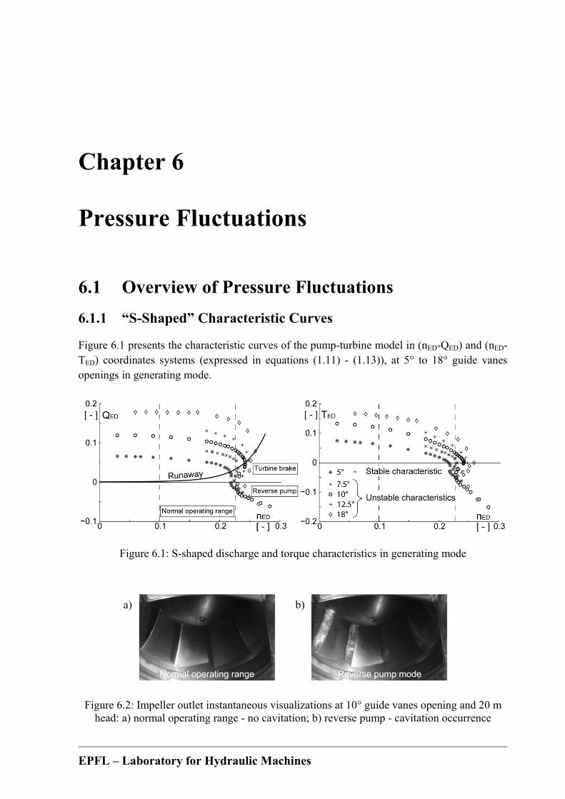
EPFL – Laboratory for Hydraulic Machines
Chapter 6
Pressure Fluctuations
6.1 Overview of Pressure Fluctuations
6.1.1 “S-Shaped” Characteristic Curves
Figure 6.1 presents the characteristic curves of the pump-turbine model in (nED-QED) and (nED-TED) coordinates systems (expressed in equations (1.11) - (1.13)), at 5° to 18° guide vanes openings in generating mode.
Figure 6.1: S-shaped discharge and torque characteristics in generating mode
Figure 6.2: Impeller outlet instantaneous visualizations at 10° guide vanes opening and 20 m head: a) normal operating range - no cavitation; b) reverse pump - cavitation occurrence
a) b)
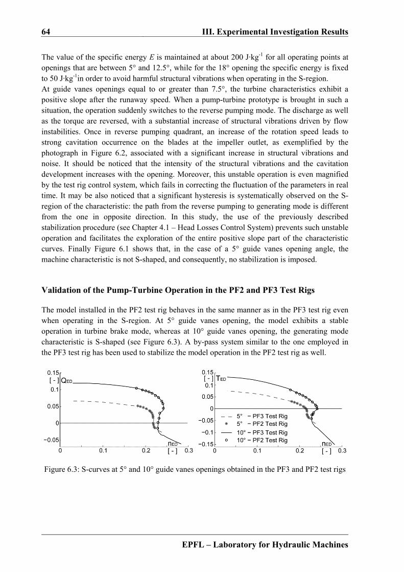
64 III. Experimental Investigation Results
EPFL – Laboratory for Hydraulic Machines
The value of the specific energy E is maintained at about 200 J·kg-1 for all operating points at openings that are between 5° and 12.5°, while for the 18° opening the specific energy is fixed to 50 J·kg-1in order to avoid harmful structural vibrations when operating in the S-region. At guide vanes openings equal to or greater than 7.5°, the turbine characteristics exhibit a positive slope after the runaway speed. When a pump-turbine prototype is brought in such a situation, the operation suddenly switches to the reverse pumping mode. The discharge as well as the torque are reversed, with a substantial increase of structural vibrations driven by flow instabilities. Once in reverse pumping quadrant, an increase of the rotation speed leads to strong cavitation occurrence on the blades at the impeller outlet, as exemplified by the photograph in Figure 6.2, associated with a significant increase in structural vibrations and noise. It should be noticed that the intensity of the structural vibrations and the cavitation development increases with the opening. Moreover, this unstable operation is even magnified by the test rig control system, which fails in correcting the fluctuation of the parameters in real time. It may be also noticed that a significant hysteresis is systematically observed on the S-region of the characteristic: the path from the reverse pumping to generating mode is different from the one in opposite direction. In this study, the use of the previously described stabilization procedure (see Chapter 4.1 – Head Losses Control System) prevents such unstable operation and facilitates the exploration of the entire positive slope part of the characteristic curves. Finally Figure 6.1 shows that, in the case of a 5° guide vanes opening angle, the machine characteristic is not S-shaped, and consequently, no stabilization is imposed.
Validation of the Pump-Turbine Operation in the PF2 and PF3 Test Rigs
The model installed in the PF2 test rig behaves in the same manner as in the PF3 test rig even when operating in the S-region. At 5° guide vanes opening, the model exhibits a stable operation in turbine brake mode, whereas at 10° guide vanes opening, the generating mode characteristic is S-shaped (see Figure 6.3). A by-pass system similar to the one employed in the PF3 test rig has been used to stabilize the model operation in the PF2 test rig as well.
Figure 6.3: S-curves at 5° and 10° guide vanes openings obtained in the PF3 and PF2 test rigs
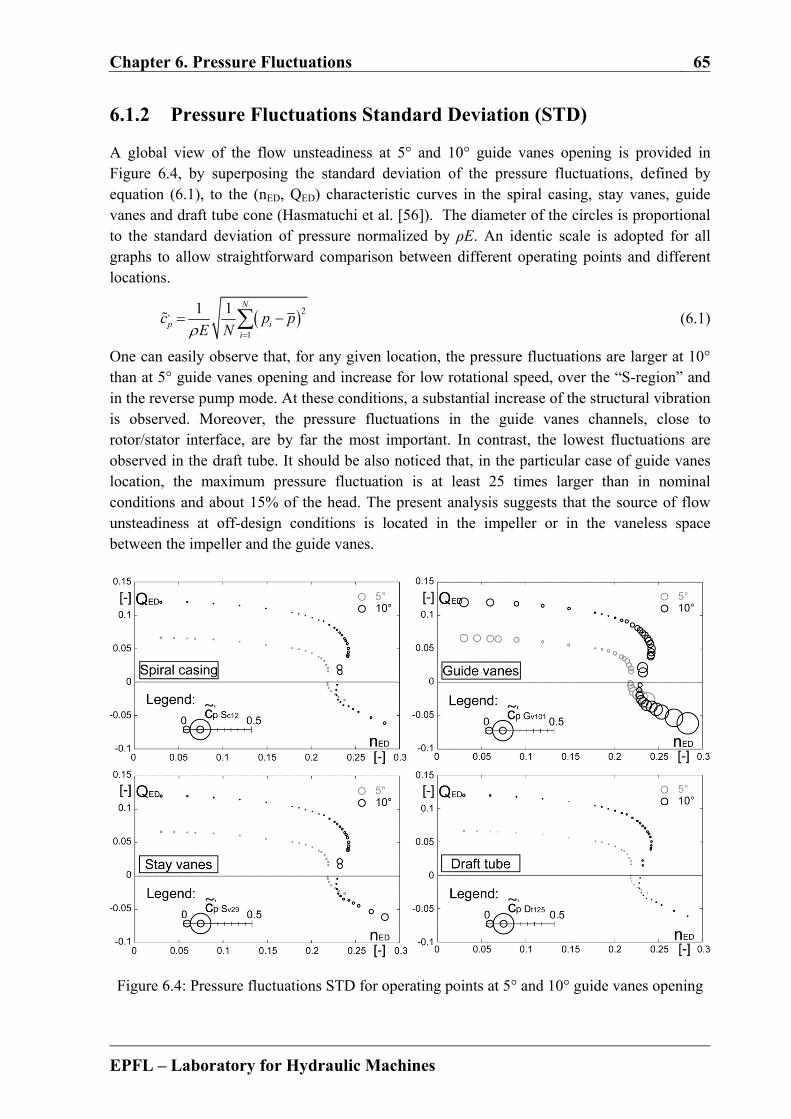
Chapter 6. Pressure Fluctuations 65
EPFL – Laboratory for Hydraulic Machines
6.1.2 Pressure Fluctuations Standard Deviation (STD)
A global view of the flow unsteadiness at 5° and 10° guide vanes opening is provided in Figure 6.4, by superposing the standard deviation of the pressure fluctuations, defined by equation (6.1), to the (nED, QED) characteristic curves in the spiral casing, stay vanes, guide vanes and draft tube cone (Hasmatuchi et al. [56]). The diameter of the circles is proportional to the standard deviation of pressure normalized by ρE. An identic scale is adopted for all graphs to allow straightforward comparison between different operating points and different locations.
2,
1
1 1 N
p ii
c p pE N
(6.1)
One can easily observe that, for any given location, the pressure fluctuations are larger at 10° than at 5° guide vanes opening and increase for low rotational speed, over the “S-region” and in the reverse pump mode. At these conditions, a substantial increase of the structural vibration is observed. Moreover, the pressure fluctuations in the guide vanes channels, close to rotor/stator interface, are by far the most important. In contrast, the lowest fluctuations are observed in the draft tube. It should be also noticed that, in the particular case of guide vanes location, the maximum pressure fluctuation is at least 25 times larger than in nominal conditions and about 15% of the head. The present analysis suggests that the source of flow unsteadiness at off-design conditions is located in the impeller or in the vaneless space between the impeller and the guide vanes.
Figure 6.4: Pressure fluctuations STD for operating points at 5° and 10° guide vanes opening
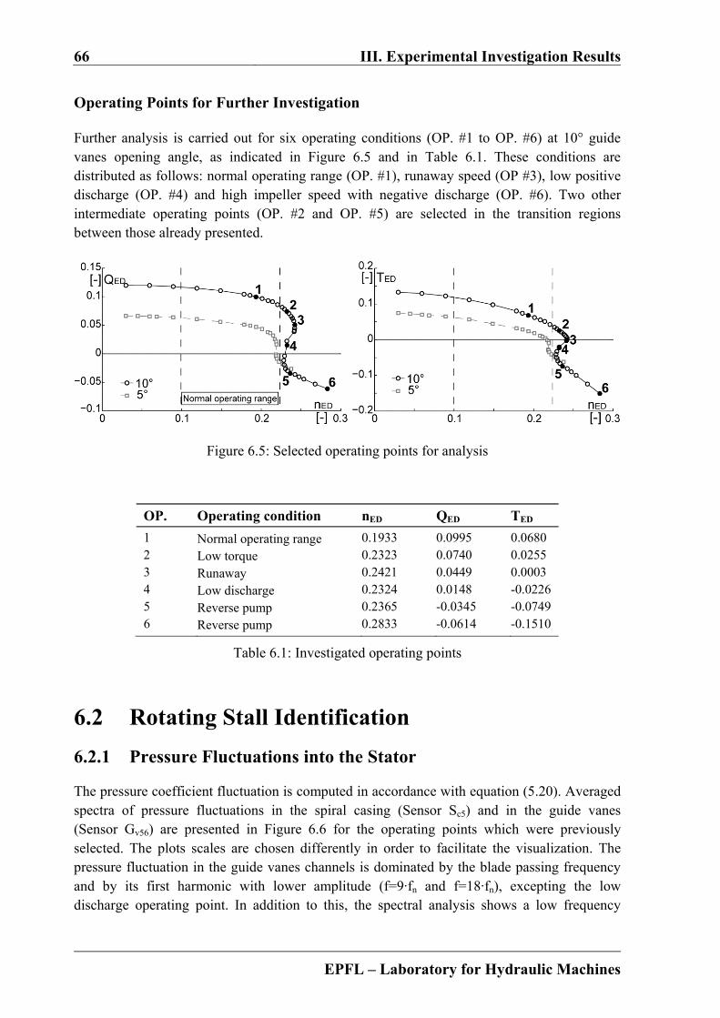
66 III. Experimental Investigation Results
EPFL – Laboratory for Hydraulic Machines
Operating Points for Further Investigation
Further analysis is carried out for six operating conditions (OP. #1 to OP. #6) at 10° guide vanes opening angle, as indicated in Figure 6.5 and in Table 6.1. These conditions are distributed as follows: normal operating range (OP. #1), runaway speed (OP #3), low positive discharge (OP. #4) and high impeller speed with negative discharge (OP. #6). Two other intermediate operating points (OP. #2 and OP. #5) are selected in the transition regions between those already presented.
Figure 6.5: Selected operating points for analysis
OP. Operating condition nED QED TED
1 Normal operating range 0.1933 0.0995 0.0680 2 Low torque 0.2323 0.0740 0.0255 3 Runaway 0.2421 0.0449 0.0003 4 Low discharge 0.2324 0.0148 -0.0226 5 Reverse pump 0.2365 -0.0345 -0.0749 6 Reverse pump 0.2833 -0.0614 -0.1510
Table 6.1: Investigated operating points
6.2 Rotating Stall Identification
6.2.1 Pressure Fluctuations into the Stator
The pressure coefficient fluctuation is computed in accordance with equation (5.20). Averaged spectra of pressure fluctuations in the spiral casing (Sensor Sc5) and in the guide vanes (Sensor Gv56) are presented in Figure 6.6 for the operating points which were previously selected. The plots scales are chosen differently in order to facilitate the visualization. The pressure fluctuation in the guide vanes channels is dominated by the blade passing frequency and by its first harmonic with lower amplitude (f=9·fn and f=18·fn), excepting the low discharge operating point. In addition to this, the spectral analysis shows a low frequency
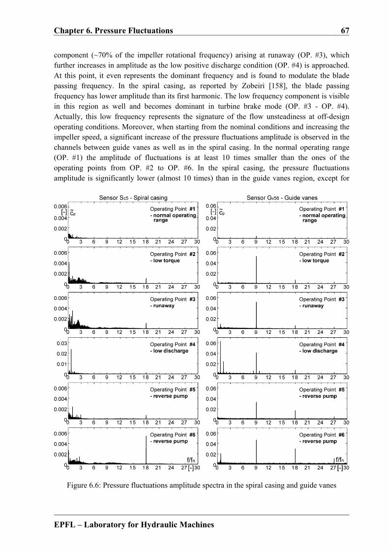
Chapter 6. Pressure Fluctuations 67
EPFL – Laboratory for Hydraulic Machines
component (~70% of the impeller rotational frequency) arising at runaway (OP. #3), which further increases in amplitude as the low positive discharge condition (OP. #4) is approached. At this point, it even represents the dominant frequency and is found to modulate the blade passing frequency. In the spiral casing, as reported by Zobeiri [158], the blade passing frequency has lower amplitude than its first harmonic. The low frequency component is visible in this region as well and becomes dominant in turbine brake mode (OP. #3 - OP. #4). Actually, this low frequency represents the signature of the flow unsteadiness at off-design operating conditions. Moreover, when starting from the nominal conditions and increasing the impeller speed, a significant increase of the pressure fluctuations amplitude is observed in the channels between guide vanes as well as in the spiral casing. In the normal operating range (OP. #1) the amplitude of fluctuations is at least 10 times smaller than the ones of the operating points from OP. #2 to OP. #6. In the spiral casing, the pressure fluctuations amplitude is significantly lower (almost 10 times) than in the guide vanes region, except for
Figure 6.6: Pressure fluctuations amplitude spectra in the spiral casing and guide vanes
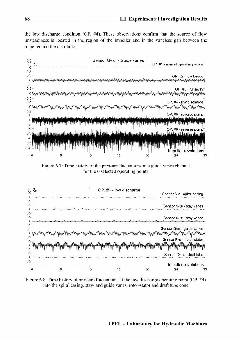
68 III. Experimental Investigation Results
EPFL – Laboratory for Hydraulic Machines
the low discharge condition (OP. #4). These observations confirm that the source of flow unsteadiness is located in the region of the impeller and in the vaneless gap between the impeller and the distributor.
Figure 6.7: Time history of the pressure fluctuations in a guide vanes channel for the 6 selected operating points
Figure 6.8: Time history of pressure fluctuations at the low discharge operating point (OP. #4) into the spiral casing, stay- and guide vanes, rotor-stator and draft tube cone
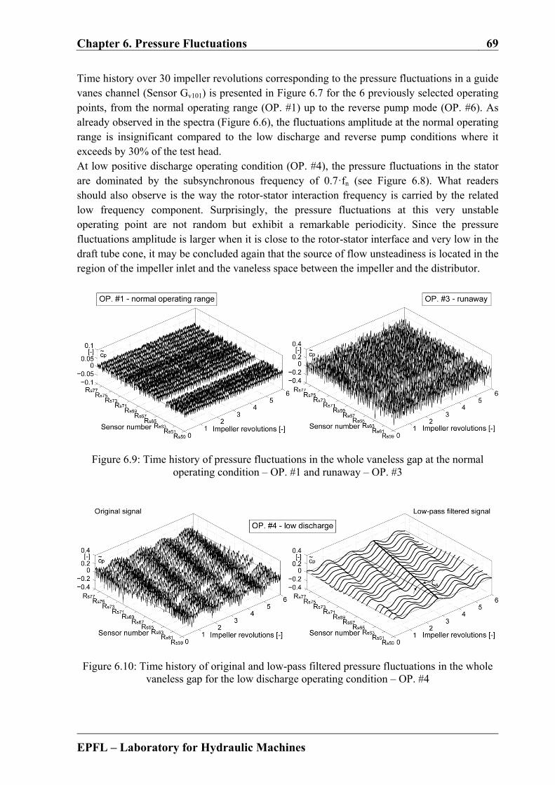
Chapter 6. Pressure Fluctuations 69
EPFL – Laboratory for Hydraulic Machines
Time history over 30 impeller revolutions corresponding to the pressure fluctuations in a guide vanes channel (Sensor Gv101) is presented in Figure 6.7 for the 6 previously selected operating points, from the normal operating range (OP. #1) up to the reverse pump mode (OP. #6). As already observed in the spectra (Figure 6.6), the fluctuations amplitude at the normal operating range is insignificant compared to the low discharge and reverse pump conditions where it exceeds by 30% of the test head. At low positive discharge operating condition (OP. #4), the pressure fluctuations in the stator are dominated by the subsynchronous frequency of 0.7·fn (see Figure 6.8). What readers should also observe is the way the rotor-stator interaction frequency is carried by the related low frequency component. Surprisingly, the pressure fluctuations at this very unstable operating point are not random but exhibit a remarkable periodicity. Since the pressure fluctuations amplitude is larger when it is close to the rotor-stator interface and very low in the draft tube cone, it may be concluded again that the source of flow unsteadiness is located in the region of the impeller inlet and the vaneless space between the impeller and the distributor.
Figure 6.9: Time history of pressure fluctuations in the whole vaneless gap at the normal operating condition – OP. #1 and runaway – OP. #3
Figure 6.10: Time history of original and low-pass filtered pressure fluctuations in the whole vaneless gap for the low discharge operating condition – OP. #4
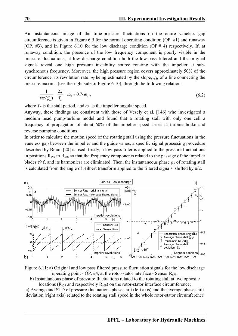
70 III. Experimental Investigation Results
EPFL – Laboratory for Hydraulic Machines
An instantaneous image of the time-pressure fluctuations on the entire vaneless gap circumference is given in Figure 6.9 for the normal operating condition (OP. #1) and runaway (OP. #3), and in Figure 6.10 for the low discharge condition (OP.# 4) respectively. If, at runaway condition, the presence of the low frequency component is poorly visible in the pressure fluctuations, at low discharge condition both the low-pass filtered and the original signals reveal one high pressure instability source rotating with the impeller at sub-synchronous frequency. Moreover, the high pressure region covers approximately 50% of the circumference, its revolution rate ωS being estimated by the slope, ϛS, of a line connecting the pressure maxima (see the right side of Figure 6.10), through the following relation:
1 20.7 ,
tan( ) S nS ST
(6.2)
where TS is the stall period, and ωn is the impeller angular speed. Anyway, these findings are consistent with those of Vesely et al. [146] who investigated a medium head pump-turbine model and found that a rotating stall with only one cell a frequency of propagation of about 60% of the impeller speed arises at turbine brake and reverse pumping conditions. In order to calculate the motion speed of the rotating stall using the pressure fluctuations in the vaneless gap between the impeller and the guide vanes, a specific signal processing procedure described by Braun [20] is used: firstly, a low-pass filter is applied to the pressure fluctuations in positions Rs59 to Rs78 so that the frequency components related to the passage of the impeller blades (9·fn and its harmonics) are eliminated. Then, the instantaneous phase φS of rotating stall is calculated from the angle of Hilbert transform applied to the filtered signals, shifted by π/2.
Figure 6.11: a) Original and low pass filtered pressure fluctuation signals for the low discharge operating point - OP. #4, at the rotor-stator interface - Sensor Rs59;
b) Instantaneous phase of pressure fluctuations related to the rotating stall at two opposite locations (Rs59 and respectively Rs69) on the rotor-stator interface circumference;
c) Average and STD of pressure fluctuations phase shift (left axis) and the average phase shift deviation (right axis) related to the rotating stall speed in the whole rotor-stator circumference
a)
b)
c)
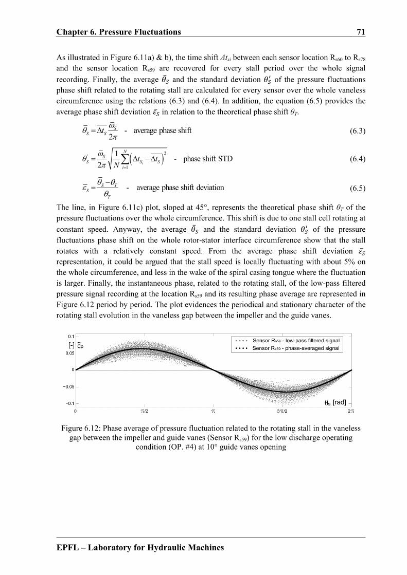
Chapter 6. Pressure Fluctuations 71
EPFL – Laboratory for Hydraulic Machines
As illustrated in Figure 6.11a) & b), the time shift Δtsi between each sensor location Rs60 to Rs78 and the sensor location Rs59 are recovered for every stall period over the whole signal
recording. Finally, the average and the standard deviation of the pressure fluctuations phase shift related to the rotating stall are calculated for every sensor over the whole vaneless circumference using the relations (6.3) and (6.4). In addition, the equation (6.5) provides the average phase shift deviation in relation to the theoretical phase shift θT.
- average phase shift2
SS St
(6.3)
2'
1
1- phase shift STD
2 i
NS
S S Si
t tN
(6.4)
- average phase shift deviationS TS
T
(6.5)
The line, in Figure 6.11c) plot, sloped at 45°, represents the theoretical phase shift θT of the pressure fluctuations over the whole circumference. This shift is due to one stall cell rotating at
constant speed. Anyway, the average and the standard deviation of the pressure fluctuations phase shift on the whole rotor-stator interface circumference show that the stall rotates with a relatively constant speed. From the average phase shift deviation representation, it could be argued that the stall speed is locally fluctuating with about 5% on the whole circumference, and less in the wake of the spiral casing tongue where the fluctuation is larger. Finally, the instantaneous phase, related to the rotating stall, of the low-pass filtered pressure signal recording at the location Rs59 and its resulting phase average are represented in Figure 6.12 period by period. The plot evidences the periodical and stationary character of the rotating stall evolution in the vaneless gap between the impeller and the guide vanes.
Figure 6.12: Phase average of pressure fluctuation related to the rotating stall in the vaneless gap between the impeller and guide vanes (Sensor Rs59) for the low discharge operating
condition (OP. #4) at 10° guide vanes opening
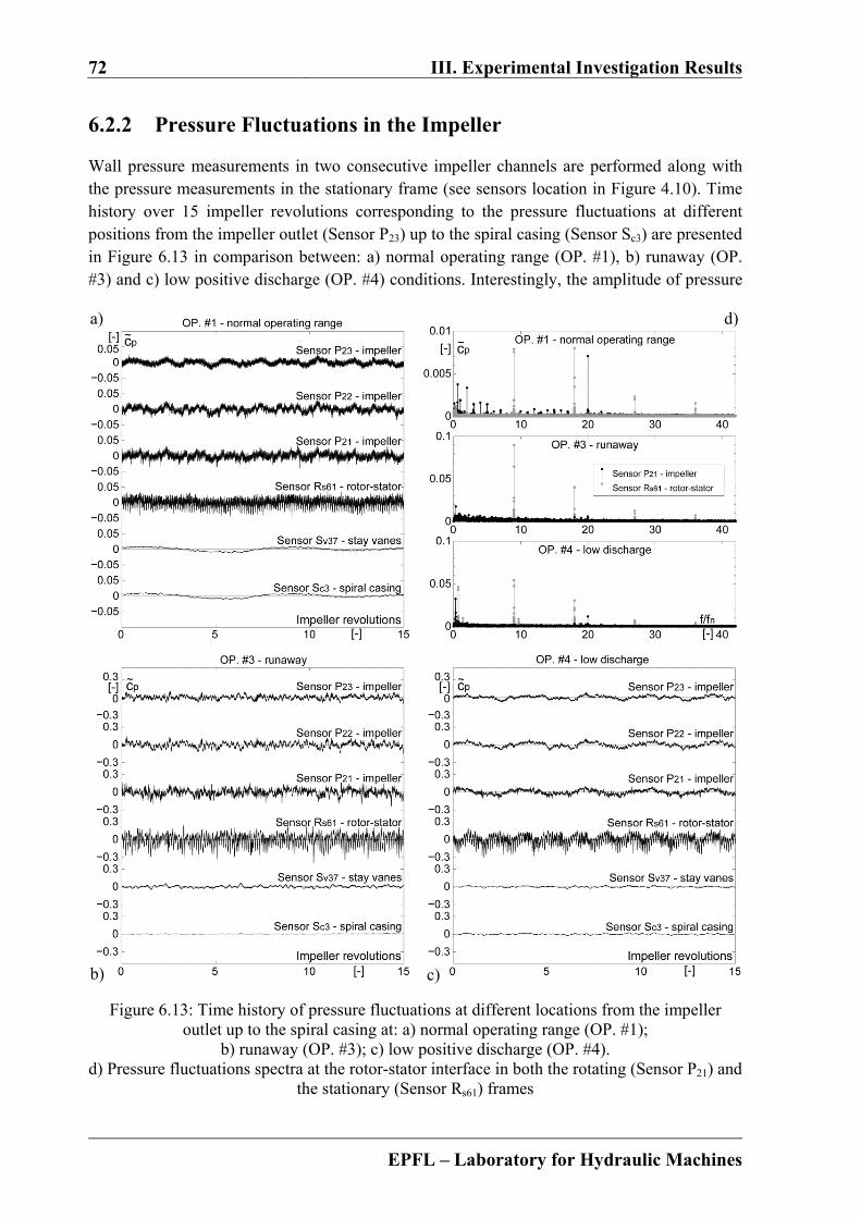
72 III. Experimental Investigation Results
EPFL – Laboratory for Hydraulic Machines
6.2.2 Pressure Fluctuations in the Impeller
Wall pressure measurements in two consecutive impeller channels are performed along with the pressure measurements in the stationary frame (see sensors location in Figure 4.10). Time history over 15 impeller revolutions corresponding to the pressure fluctuations at different positions from the impeller outlet (Sensor P23) up to the spiral casing (Sensor Sc3) are presented in Figure 6.13 in comparison between: a) normal operating range (OP. #1), b) runaway (OP. #3) and c) low positive discharge (OP. #4) conditions. Interestingly, the amplitude of pressure
Figure 6.13: Time history of pressure fluctuations at different locations from the impeller outlet up to the spiral casing at: a) normal operating range (OP. #1);
b) runaway (OP. #3); c) low positive discharge (OP. #4). d) Pressure fluctuations spectra at the rotor-stator interface in both the rotating (Sensor P21) and
the stationary (Sensor Rs61) frames
a)
b) c)
d)
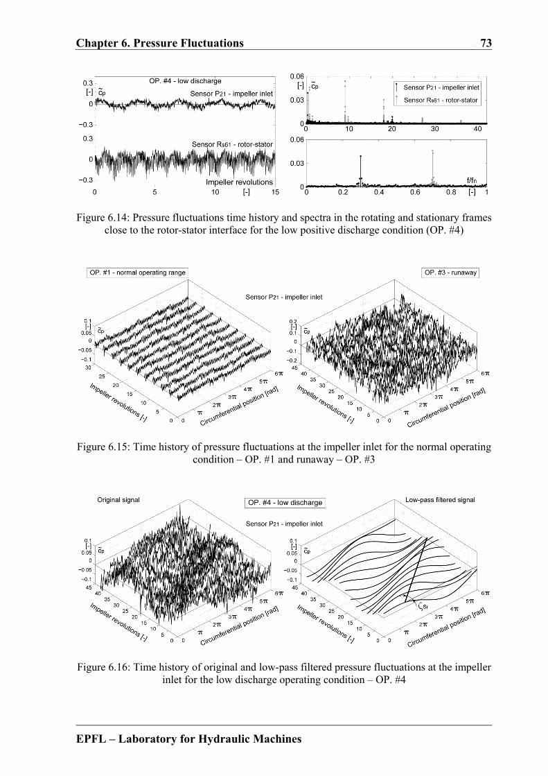
Chapter 6. Pressure Fluctuations 73
EPFL – Laboratory for Hydraulic Machines
Figure 6.14: Pressure fluctuations time history and spectra in the rotating and stationary frames close to the rotor-stator interface for the low positive discharge condition (OP. #4)
Figure 6.15: Time history of pressure fluctuations at the impeller inlet for the normal operating condition – OP. #1 and runaway – OP. #3
Figure 6.16: Time history of original and low-pass filtered pressure fluctuations at the impeller inlet for the low discharge operating condition – OP. #4
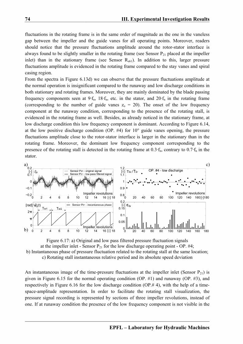
74 III. Experimental Investigation Results
EPFL – Laboratory for Hydraulic Machines
fluctuations in the rotating frame is in the same order of magnitude as the one in the vaneless gap between the impeller and the guide vanes for all operating points. Moreover, readers should notice that the pressure fluctuations amplitude around the rotor-stator interface is always found to be slightly smaller in the rotating frame (see Sensor P21 placed at the impeller inlet) than in the stationary frame (see Sensor Rs61). In addition to this, larger pressure fluctuations amplitude is evidenced in the rotating frame compared to the stay vanes and spiral casing region. From the spectra in Figure 6.13d) we can observe that the pressure fluctuations amplitude at the normal operation is insignificant compared to the runaway and low discharge conditions in both stationary and rotating frames. Moreover, they are mainly dominated by the blade passing frequency components seen at 9·fn, 18·fn, etc. in the stator, and 20·fn in the rotating frame (corresponding to the number of guide vanes zo = 20). The onset of the low frequency component at the runaway condition, corresponding to the presence of the rotating stall, is evidenced in the rotating frame as well. Besides, as already noticed in the stationary frame, at low discharge condition this low frequency component is dominant. According to Figure 6.14, at the low positive discharge condition (OP. #4) for 10° guide vanes opening, the pressure fluctuations amplitude close to the rotor-stator interface is larger in the stationary than in the rotating frame. Moreover, the dominant low frequency component corresponding to the presence of the rotating stall is detected in the rotating frame at 0.3·fn, contrary to 0.7·fn in the stator.
Figure 6.17: a) Original and low pass filtered pressure fluctuation signals at the impeller inlet - Sensor P21 for the low discharge operating point - OP. #4;
b) Instantaneous phase of pressure fluctuation related to the rotating stall at the same location; c) Rotating stall instantaneous relative period and its absolute speed deviation
An instantaneous image of the time-pressure fluctuations at the impeller inlet (Sensor P21) is given in Figure 6.15 for the normal operating condition (OP. #1) and runaway (OP. #3), and respectively in Figure 6.16 for the low discharge condition (OP.# 4), with the help of a time-space-amplitude representation. In order to facilitate the rotating stall visualization, the pressure signal recording is represented by sections of three impeller revolutions, instead of one. If at runaway condition the presence of the low frequency component is not visible in the
a)
b)
c)
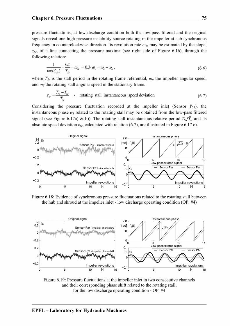
Chapter 6. Pressure Fluctuations 75
EPFL – Laboratory for Hydraulic Machines
pressure fluctuations, at low discharge condition both the low-pass filtered and the original signals reveal one high pressure instability source rotating in the impeller at sub-synchronous frequency in counterclockwise direction. Its revolution rate ωSr may be estimated by the slope, ϛSr, of a line connecting the pressure maxima (see right side of Figure 6.16), through the following relation:
1 60.3 ,
tan( ) Sr n n SSr SrT
(6.6)
where TSr is the stall period in the rotating frame referential, ωn the impeller angular speed, and ωS the rotating stall angular speed in the stationary frame.
- rotating stall instantaneous speed deviationSr SrSr
Sr
T T
T
(6.7)
Considering the pressure fluctuation recorded at the impeller inlet (Sensor P21), the instantaneous phase φS related to the rotating stall may be obtained from the low-pass filtered signal (see Figure 6.17a) & b)). The rotating stall instantaneous relative period / and its absolute speed deviation εSr, calculated with relation (6.7), are illustrated in Figure 6.17 c).
Figure 6.18: Evidence of synchronous pressure fluctuations related to the rotating stall between the hub and shroud at the impeller inlet - low discharge operating condition (OP. #4)
Figure 6.19: Pressure fluctuations at the impeller inlet in two consecutive channels and their corresponding phase shift related to the rotating stall,
for the low discharge operating condition - OP. #4
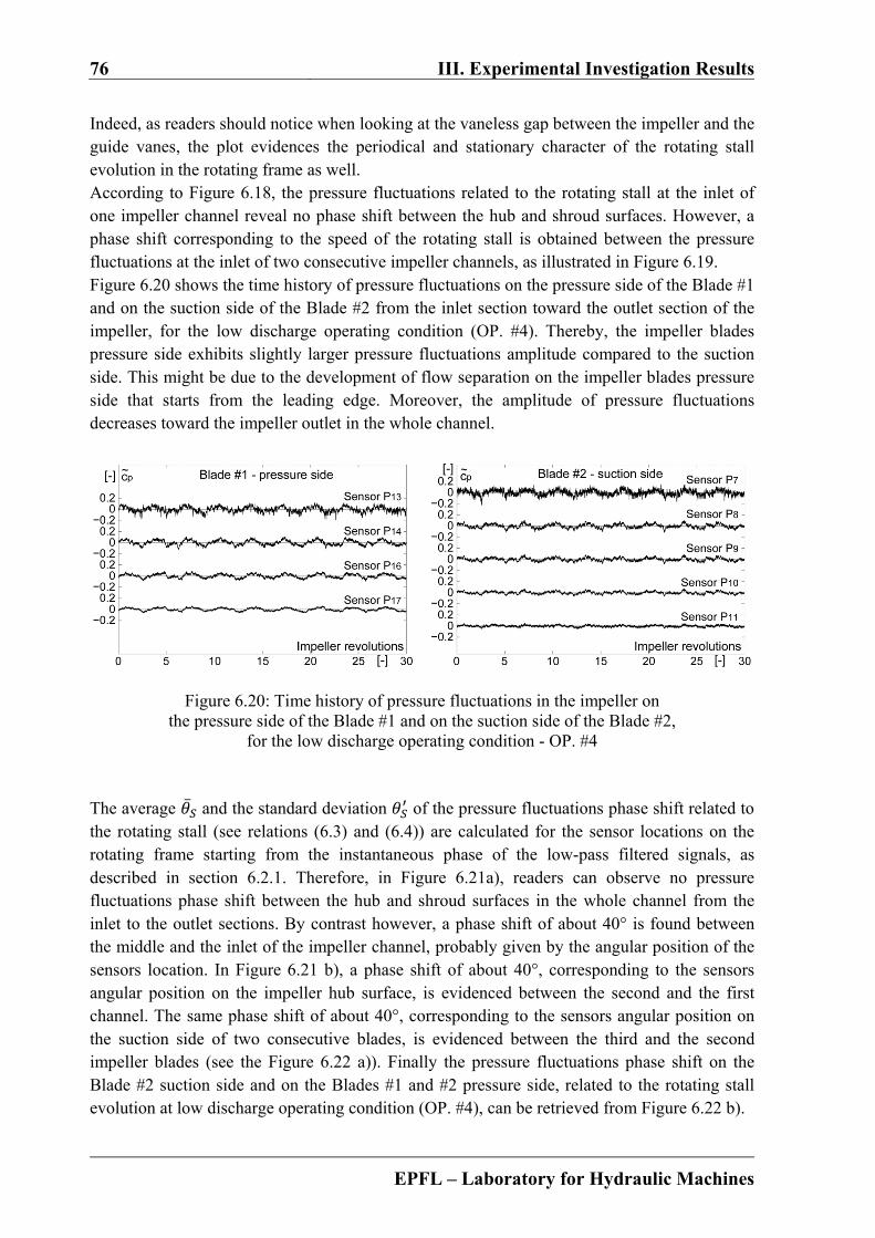
76 III. Experimental Investigation Results
EPFL – Laboratory for Hydraulic Machines
Indeed, as readers should notice when looking at the vaneless gap between the impeller and the guide vanes, the plot evidences the periodical and stationary character of the rotating stall evolution in the rotating frame as well. According to Figure 6.18, the pressure fluctuations related to the rotating stall at the inlet of one impeller channel reveal no phase shift between the hub and shroud surfaces. However, a phase shift corresponding to the speed of the rotating stall is obtained between the pressure fluctuations at the inlet of two consecutive impeller channels, as illustrated in Figure 6.19. Figure 6.20 shows the time history of pressure fluctuations on the pressure side of the Blade #1 and on the suction side of the Blade #2 from the inlet section toward the outlet section of the impeller, for the low discharge operating condition (OP. #4). Thereby, the impeller blades pressure side exhibits slightly larger pressure fluctuations amplitude compared to the suction side. This might be due to the development of flow separation on the impeller blades pressure side that starts from the leading edge. Moreover, the amplitude of pressure fluctuations decreases toward the impeller outlet in the whole channel.
Figure 6.20: Time history of pressure fluctuations in the impeller on the pressure side of the Blade #1 and on the suction side of the Blade #2,
for the low discharge operating condition - OP. #4
The average and the standard deviation of the pressure fluctuations phase shift related to the rotating stall (see relations (6.3) and (6.4)) are calculated for the sensor locations on the rotating frame starting from the instantaneous phase of the low-pass filtered signals, as described in section 6.2.1. Therefore, in Figure 6.21a), readers can observe no pressure fluctuations phase shift between the hub and shroud surfaces in the whole channel from the inlet to the outlet sections. By contrast however, a phase shift of about 40° is found between the middle and the inlet of the impeller channel, probably given by the angular position of the sensors location. In Figure 6.21 b), a phase shift of about 40°, corresponding to the sensors angular position on the impeller hub surface, is evidenced between the second and the first channel. The same phase shift of about 40°, corresponding to the sensors angular position on the suction side of two consecutive blades, is evidenced between the third and the second impeller blades (see the Figure 6.22 a)). Finally the pressure fluctuations phase shift on the Blade #2 suction side and on the Blades #1 and #2 pressure side, related to the rotating stall evolution at low discharge operating condition (OP. #4), can be retrieved from Figure 6.22 b).
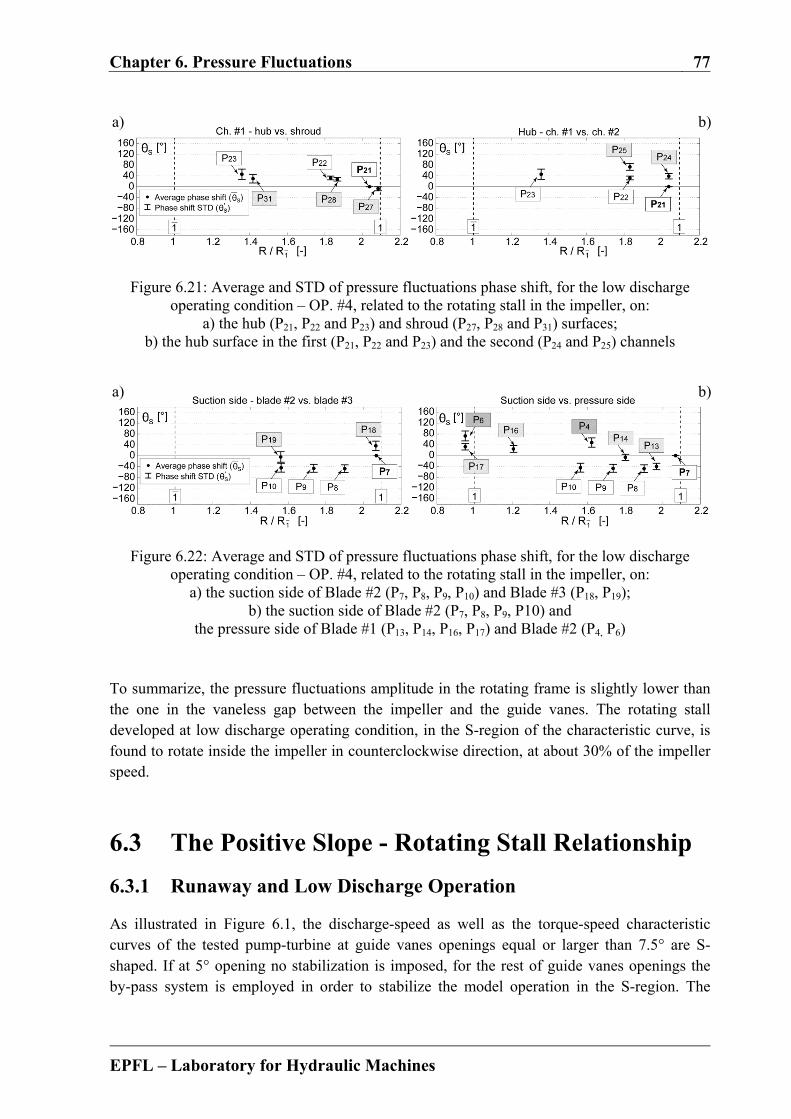
Chapter 6. Pressure Fluctuations 77
EPFL – Laboratory for Hydraulic Machines
Figure 6.21: Average and STD of pressure fluctuations phase shift, for the low discharge operating condition – OP. #4, related to the rotating stall in the impeller, on:
a) the hub (P21, P22 and P23) and shroud (P27, P28 and P31) surfaces; b) the hub surface in the first (P21, P22 and P23) and the second (P24 and P25) channels
Figure 6.22: Average and STD of pressure fluctuations phase shift, for the low discharge operating condition – OP. #4, related to the rotating stall in the impeller, on:
a) the suction side of Blade #2 (P7, P8, P9, P10) and Blade #3 (P18, P19); b) the suction side of Blade #2 (P7, P8, P9, P10) and
the pressure side of Blade #1 (P13, P14, P16, P17) and Blade #2 (P4, P6) To summarize, the pressure fluctuations amplitude in the rotating frame is slightly lower than the one in the vaneless gap between the impeller and the guide vanes. The rotating stall developed at low discharge operating condition, in the S-region of the characteristic curve, is found to rotate inside the impeller in counterclockwise direction, at about 30% of the impeller speed.
6.3 The Positive Slope - Rotating Stall Relationship
6.3.1 Runaway and Low Discharge Operation
As illustrated in Figure 6.1, the discharge-speed as well as the torque-speed characteristic curves of the tested pump-turbine at guide vanes openings equal or larger than 7.5° are S-shaped. If at 5° opening no stabilization is imposed, for the rest of guide vanes openings the by-pass system is employed in order to stabilize the model operation in the S-region. The
a) b)
a) b)
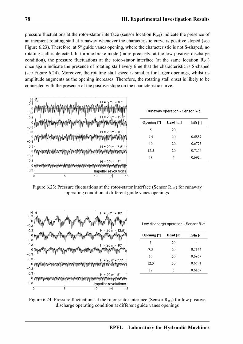
78 III. Experimental Investigation Results
EPFL – Laboratory for Hydraulic Machines
pressure fluctuations at the rotor-stator interface (sensor location Rs61) indicate the presence of an incipient rotating stall at runaway whenever the characteristic curve is positive sloped (see Figure 6.23). Therefore, at 5° guide vanes opening, where the characteristic is not S-shaped, no rotating stall is detected. In turbine brake mode (more precisely, at the low positive discharge condition), the pressure fluctuations at the rotor-stator interface (at the same location Rs61) once again indicate the presence of rotating stall every time that the characteristic is S-shaped (see Figure 6.24). Moreover, the rotating stall speed is smaller for larger openings, whilst its amplitude augments as the opening increases. Therefore, the rotating stall onset is likely to be connected with the presence of the positive slope on the characteristic curve.
Figure 6.23: Pressure fluctuations at the rotor-stator interface (Sensor Rs61) for runaway operating condition at different guide vanes openings
Figure 6.24: Pressure fluctuations at the rotor-stator interface (Sensor Rs61) for low positive discharge operating condition at different guide vanes openings

Chapter 6. Pressure Fluctuations 79
EPFL – Laboratory for Hydraulic Machines
6.3.2 Head Influence on the Operation Stability
As illustrated in the plots of Figure 6.25, the shape of the characteristic curves and the operation stability for both 5° and 10° guide vanes opening are unaffected by the change of the operation head in the range between 16 and 25 m. Indeed, the change of test head is made with respect to the similarity rules (6.8). As can be observed by looking at the plots from the bottom side of Figure 6.25, the model characteristic remains unchanged for 10° guide vanes opening
Figure 6.25: Head influence on the characteristic curves shape and the operation stability
Figure 6.26: Head influence on pressure fluctuations at the rotor-stator interface (Sensor Rs61) for the low discharge operating conditions at 5° and 10° guide vanes opening angles
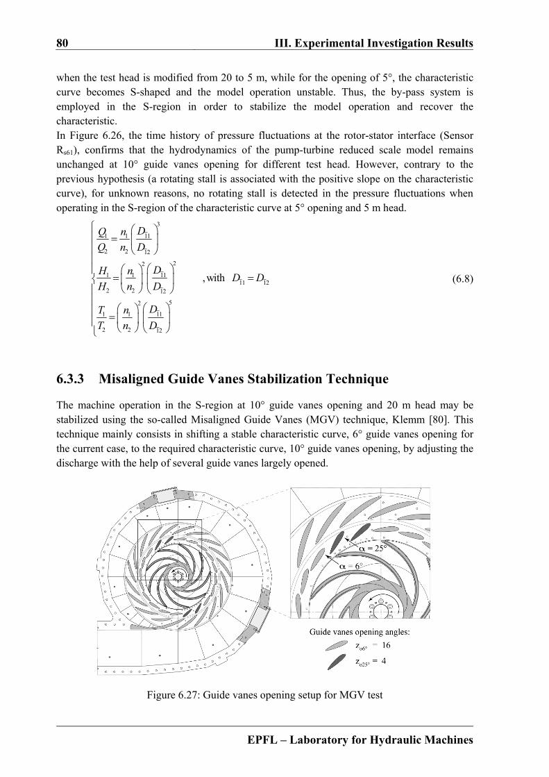
80 III. Experimental Investigation Results
EPFL – Laboratory for Hydraulic Machines
when the test head is modified from 20 to 5 m, while for the opening of 5°, the characteristic curve becomes S-shaped and the model operation unstable. Thus, the by-pass system is employed in the S-region in order to stabilize the model operation and recover the characteristic. In Figure 6.26, the time history of pressure fluctuations at the rotor-stator interface (Sensor Rs61), confirms that the hydrodynamics of the pump-turbine reduced scale model remains unchanged at 10° guide vanes opening for different test head. However, contrary to the previous hypothesis (a rotating stall is associated with the positive slope on the characteristic curve), for unknown reasons, no rotating stall is detected in the pressure fluctuations when operating in the S-region of the characteristic curve at 5° opening and 5 m head.
3
1 1 11
2 2 12
22
1 1 1111 12
2 2 12
52
1 1 11
2 2 12
,with
DQ n
Q n D
DH nD D
H n D
DT n
T n D
(6.8)
6.3.3 Misaligned Guide Vanes Stabilization Technique
The machine operation in the S-region at 10° guide vanes opening and 20 m head may be stabilized using the so-called Misaligned Guide Vanes (MGV) technique, Klemm [80]. This technique mainly consists in shifting a stable characteristic curve, 6° guide vanes opening for the current case, to the required characteristic curve, 10° guide vanes opening, by adjusting the discharge with the help of several guide vanes largely opened.
Figure 6.27: Guide vanes opening setup for MGV test

Chapter 6. Pressure Fluctuations 81
EPFL – Laboratory for Hydraulic Machines
Thereby, as illustrated in Figure 6.27, zo6° = 16 guide vanes are set to 6° opening, while the rest of zo25° = 4 guide vanes are opened at 25° in such way that they form two opposite channels, thus avoiding the introduction of an additional radial force to the impeller. The resulting discharge and torque characteristics are given in Figure 6.28. The original impeller speed and head for all operating points at 10° guide vanes opening angle, and for runaway condition, are kept unchanged. It can be observed that the machine characteristic using the MGV technique is not any more S-shaped. Consequently, since the operation in the S-region is stable, the by-pass system has not been employed. Moreover, the pressure fluctuations at the rotor-stator interface (Sensor Rs77) show no rotating stall development in the S-region (see Figure 6.29). Empirically, the discharge that is necessary in order to shift the operating point at 6° opening to the target one at 10° opening for the same impeller speed and head could be calculated as:
10 6 6 25 25 6 25 6 25 25 6 25 6 , withch ch ch ch chz Q z Q z Q z Q z Q (6.9)
6 25 6 25 25 6 , where:ch ch ch ch chz z z z z (6.10)
zch = 20 - total number of guide vanes channels zchx° - number of guide vanes channels of x° opening zchx°-y° - number of guide vanes channels adjacent to respectively x° and y° openings Qx° - discharge of one guide vanes channel of x° opening at the same impeller speed as the target operating point Qx°-y° - discharge of one guide vanes channel adjacent to respectively x° and y° openings at the same impeller speed as the target operating point
Figure 6.28: Characteristic curves of the model for 10° opening with and without MGV
Figure 6.29: Time history of pressure fluctuations at the rotor-stator interface (Sensor Rs77) for the low discharge operating condition at 10° opening with and without MGV stabilization

82 III. Experimental Investigation Results
EPFL – Laboratory for Hydraulic Machines
Furthermore, Shao [128] proposed and validated empirical formulae that allow researchers to compute the whole generating mode pump-turbine internal characteristics with MGV, and that are based on the classical theory of turbomachinery and the original model characteristic curves without MGV. Nevertheless, since the flow conditions in the channels adjacent to different openings (in our case 6° - 25° and vice versa) are not easy to predict, a theoretical formulation that describes the characteristic curve with MGV is not obvious. In addition to this, the same characteristic curve without MGV can be obtained from a multitude of MGV configurations. Therefore, this stabilization method is not considered adequate for the current experimental study.
6.3.4 Transient Test over the S-region of the Characteristic
A transient test over the S-region of the pump-turbine reduced scale model characteristic curve at 10° guide vanes opening is conducted. The resulting torque-speed characteristic of transient test is superposed to the steady state characteristic in Figure 6.30. The discharge-speed characteristic of the transient test is not represented because the discharge fluctuation measurement is not available. As illustrated in Figure 6.31, starting from a stable operating point in the vicinity of runaway speed outside the positive slope of the characteristic, the impeller rotational speed is slightly increased in order to reach the runaway condition. Up to about 28 seconds, the impeller mean torque stays almost constant at around the zero value (speed no-load condition); the pressure fluctuation amplitude at the rotor-stator interface (Sensor Rs60) remains unchanged as well. During the next 10 seconds the development of flow instabilities inside the model induces a strong decrease of the impeller torque, associated with fluctuations of the impeller speed. At the same time, the pressure measurement indicates an increase of the mean value and a reduction of the fluctuation amplitude. This corresponds to the operation carried out on the positive sloped section of the characteristic, when the discharge is reversed. Once in reverse pump mode (from 38 to 100 seconds), the impeller speed, impeller torque and the pressure fluctuations do not change any more.
Figure 6.30: Discharge-speed and torque-speed characteristic curves of the pump-turbine reduced scale model at 10° guide vanes opening obtained from steady state and transient tests
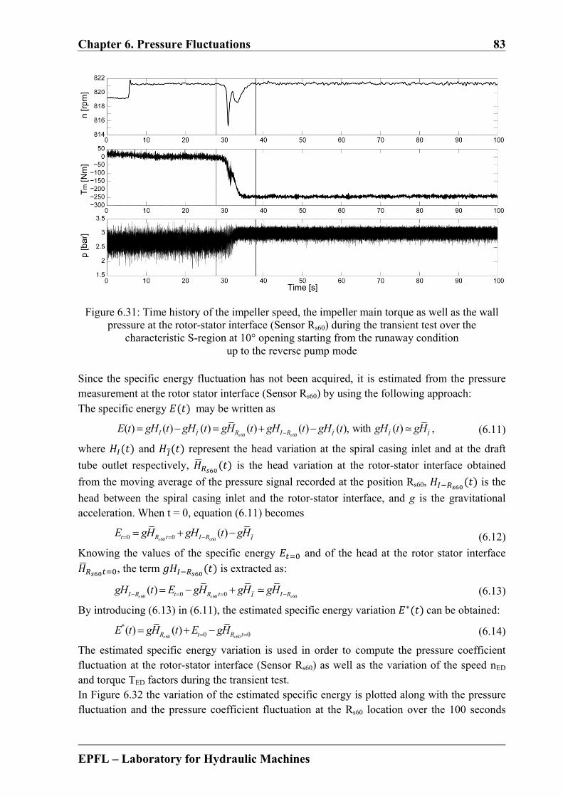
Chapter 6. Pressure Fluctuations 83
EPFL – Laboratory for Hydraulic Machines
Figure 6.31: Time history of the impeller speed, the impeller main torque as well as the wall pressure at the rotor-stator interface (Sensor Rs60) during the transient test over the
characteristic S-region at 10° opening starting from the runaway condition up to the reverse pump mode
Since the specific energy fluctuation has not been acquired, it is estimated from the pressure measurement at the rotor stator interface (Sensor Rs60) by using the following approach: The specific energy may be written as
60 60
( ) ( ) ( ) ( ) ( ) ( ), with ( ) ,s sI R I RI I I IE t gH t gH t gH t gH t gH t gH t gH (6.11)
where and represent the head variation at the spiral casing inlet and at the draft
tube outlet respectively, is the head variation at the rotor-stator interface obtained
from the moving average of the pressure signal recorded at the position Rs60, is the
head between the spiral casing inlet and the rotor-stator interface, and g is the gravitational acceleration. When t = 0, equation (6.11) becomes
60 600 0 ( )s st R t I R IE gH gH t gH (6.12)
Knowing the values of the specific energy and of the head at the rotor stator interface , the term is extracted as:
60 60 600 0( )s s sI R t R t I RIgH t E gH gH gH (6.13)
By introducing (6.13) in (6.11), the estimated specific energy variation ∗can be obtained:
60 60
*0 0( ) ( )
s sR t R tE t gH t E gH (6.14)
The estimated specific energy variation is used in order to compute the pressure coefficient fluctuation at the rotor-stator interface (Sensor Rs60) as well as the variation of the speed nED and torque TED factors during the transient test. In Figure 6.32 the variation of the estimated specific energy is plotted along with the pressure fluctuation and the pressure coefficient fluctuation at the Rs60 location over the 100 seconds
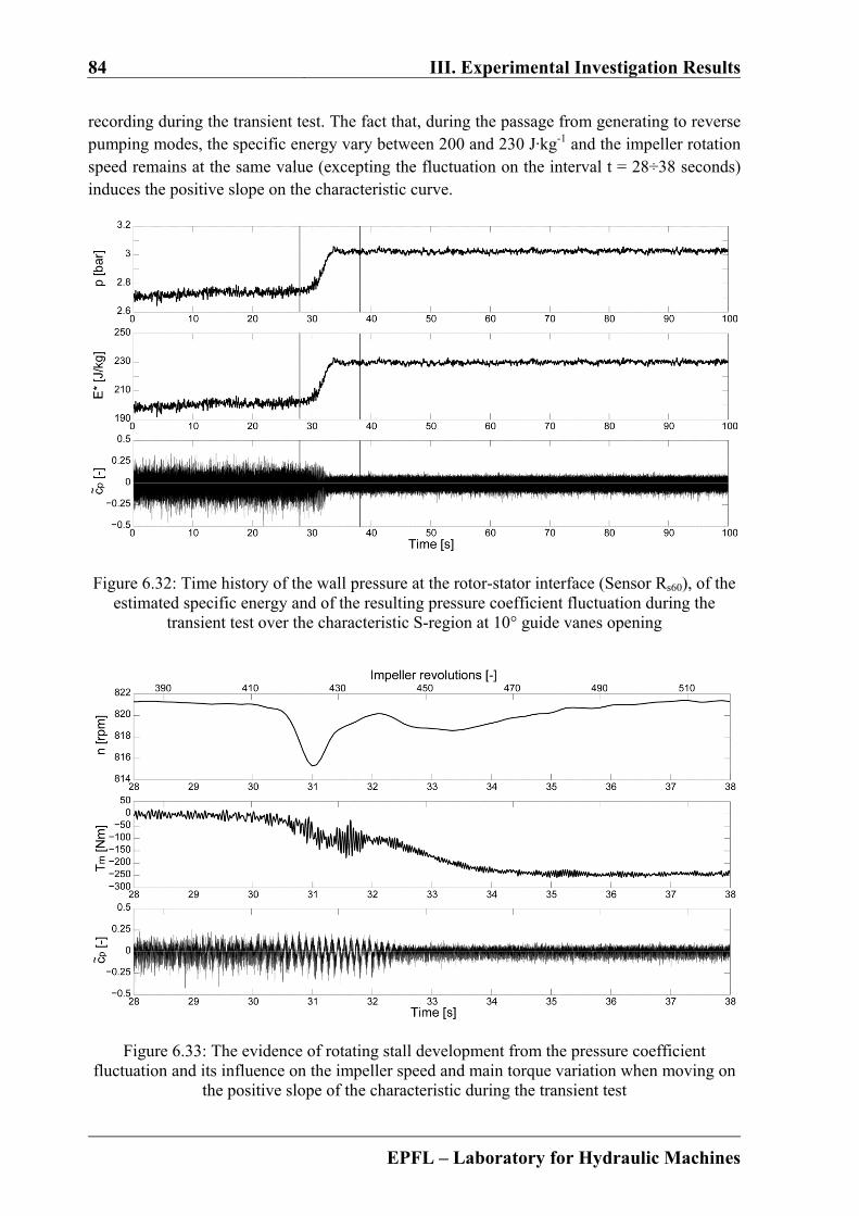
84 III. Experimental Investigation Results
EPFL – Laboratory for Hydraulic Machines
recording during the transient test. The fact that, during the passage from generating to reverse pumping modes, the specific energy vary between 200 and 230 J·kg-1 and the impeller rotation speed remains at the same value (excepting the fluctuation on the interval t = 28÷38 seconds) induces the positive slope on the characteristic curve.
Figure 6.32: Time history of the wall pressure at the rotor-stator interface (Sensor Rs60), of the estimated specific energy and of the resulting pressure coefficient fluctuation during the
transient test over the characteristic S-region at 10° guide vanes opening
Figure 6.33: The evidence of rotating stall development from the pressure coefficient fluctuation and its influence on the impeller speed and main torque variation when moving on
the positive slope of the characteristic during the transient test
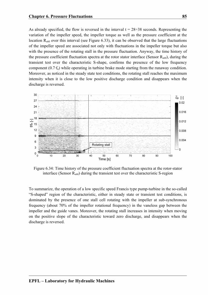
Chapter 6. Pressure Fluctuations 85
EPFL – Laboratory for Hydraulic Machines
As already specified, the flow is reversed in the interval t = 28÷38 seconds. Representing the variation of the impeller speed, the impeller torque as well as the pressure coefficient at the location Rs60 over this interval (see Figure 6.33), it can be observed that the large fluctuations of the impeller speed are associated not only with fluctuations in the impeller torque but also with the presence of the rotating stall in the pressure fluctuation. Anyway, the time history of the pressure coefficient fluctuation spectra at the rotor stator interface (Sensor Rs60), during the transient test over the characteristic S-shape, confirms the presence of the low frequency component (0.7·fn) while operating in turbine brake mode starting from the runaway condition. Moreover, as noticed in the steady state test conditions, the rotating stall reaches the maximum intensity when it is close to the low positive discharge condition and disappears when the discharge is reversed.
Figure 6.34: Time history of the pressure coefficient fluctuation spectra at the rotor-stator interface (Sensor Rs60) during the transient test over the characteristic S-region
To summarize, the operation of a low specific speed Francis type pump-turbine in the so-called “S-shaped” region of the characteristic, either in steady state or transient test conditions, is dominated by the presence of one stall cell rotating with the impeller at sub-synchronous frequency (about 70% of the impeller rotational frequency) in the vaneless gap between the impeller and the guide vanes. Moreover, the rotating stall increases in intensity when moving on the positive slope of the characteristic toward zero discharge, and disappears when the discharge is reversed.

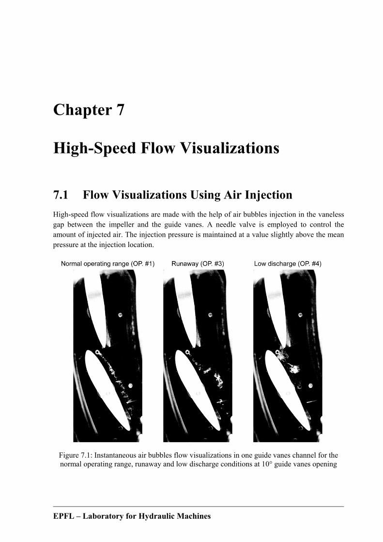
EPFL – Laboratory for Hydraulic Machines
Chapter 7
High-Speed Flow Visualizations
7.1 Flow Visualizations Using Air Injection
High-speed flow visualizations are made with the help of air bubbles injection in the vaneless gap between the impeller and the guide vanes. A needle valve is employed to control the amount of injected air. The injection pressure is maintained at a value slightly above the mean pressure at the injection location.
Figure 7.1: Instantaneous air bubbles flow visualizations in one guide vanes channel for the normal operating range, runaway and low discharge conditions at 10° guide vanes opening

88 III. Experimental Investigation Results
EPFL – Laboratory for Hydraulic Machines
Figure 7.2: Superposition of air bubbles visualizations in one guide vanes channel during 3 impeller revolutions for the normal operating range, runaway and low discharge
conditions at 10° guide vanes opening, [53] Assuming that air bubbles fairly follow the streamlines with almost no effect on the flow itself, Figure 7.1 illustrates arbitrary instantaneous captures of the flow pattern in the guide vanes region for the normal operating range (OP. #1), runaway (OP. #3) and low discharge (OP. #4) conditions at 10° guide vanes opening and 20 m head. To assess the flow trajectory in the guide vanes channel, the sum of images captured during 3 impeller revolutions at 1000 fps is given in Figure 7.2 for the same operating points OP. #1, #3 and #4. Therefore, at the normal operating range (OP #1) the trajectory of air bubbles is straight inside the guide vanes channel, and becomes slightly unstable in the wake of the neighboring guide vane. At runaway (OP. #3), the flow becomes more disturbed, as evidenced by the scatter of air bubbles, whereas at low discharge (OP. #4) and during the passage of the rotating stall, part of injected air is found upstream to the injection site, suggesting the occurrence of backflow. As shown in Figure 6.10, one stall cell travels with the impeller at sub-synchronous speed at low discharge operating condition (OP. #4). Assuming a constant rotating stall speed and the same induced pressure fluctuations amplitude in the whole vaneless ring, a time distribution of the phenomenon can be represented as a space distribution by placing images for one rotating stall period with appropriate phase shift. This allows us to obtain a synthetic instantaneous view of the flow state in the entire guide vanes circumference. A specific image processing is performed on high-speed movie, at low discharge operating point (OP. #4). Figure 7.3 presents the schematic representation of image processing operations carried out in order to create the synthetic flow visualization over the entire guide vanes circumference. The programming is performed within MATLAB environment.
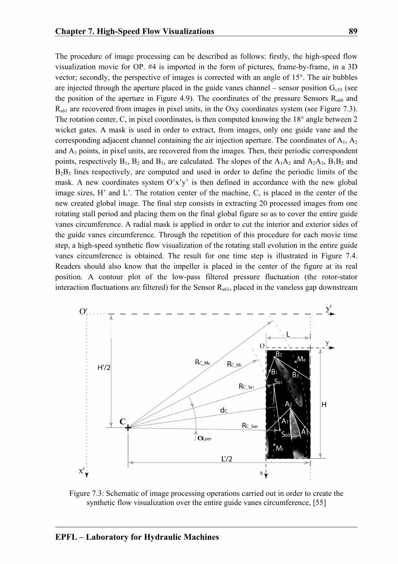
Chapter 7. High-Speed Flow Visualizations 89
EPFL – Laboratory for Hydraulic Machines
The procedure of image processing can be described as follows: firstly, the high-speed flow visualization movie for OP. #4 is imported in the form of pictures, frame-by-frame, in a 3D vector; secondly, the perspective of images is corrected with an angle of 15°. The air bubbles are injected through the aperture placed in the guide vanes channel – sensor position Gv55 (see the position of the aperture in Figure 4.9). The coordinates of the pressure Sensors Rs60 and Rs61 are recovered from images in pixel units, in the Oxy coordinates system (see Figure 7.3). The rotation center, C, in pixel coordinates, is then computed knowing the 18° angle between 2 wicket gates. A mask is used in order to extract, from images, only one guide vane and the corresponding adjacent channel containing the air injection aperture. The coordinates of A1, A2 and A3 points, in pixel units, are recovered from the images. Then, their periodic correspondent points, respectively B1, B2 and B3, are calculated. The slopes of the A1A2 and A2A3, B1B2 and B2B3 lines respectively, are computed and used in order to define the periodic limits of the mask. A new coordinates system O’x’y’ is then defined in accordance with the new global image sizes, H’ and L’. The rotation center of the machine, C, is placed in the center of the new created global image. The final step consists in extracting 20 processed images from one rotating stall period and placing them on the final global figure so as to cover the entire guide vanes circumference. A radial mask is applied in order to cut the interior and exterior sides of the guide vanes circumference. Through the repetition of this procedure for each movie time step, a high-speed synthetic flow visualization of the rotating stall evolution in the entire guide vanes circumference is obtained. The result for one time step is illustrated in Figure 7.4. Readers should also know that the impeller is placed in the center of the figure at its real position. A contour plot of the low-pass filtered pressure fluctuation (the rotor-stator interaction fluctuations are filtered) for the Sensor Rs61, placed in the vaneless gap downstream
Figure 7.3: Schematic of image processing operations carried out in order to create the synthetic flow visualization over the entire guide vanes circumference, [55]
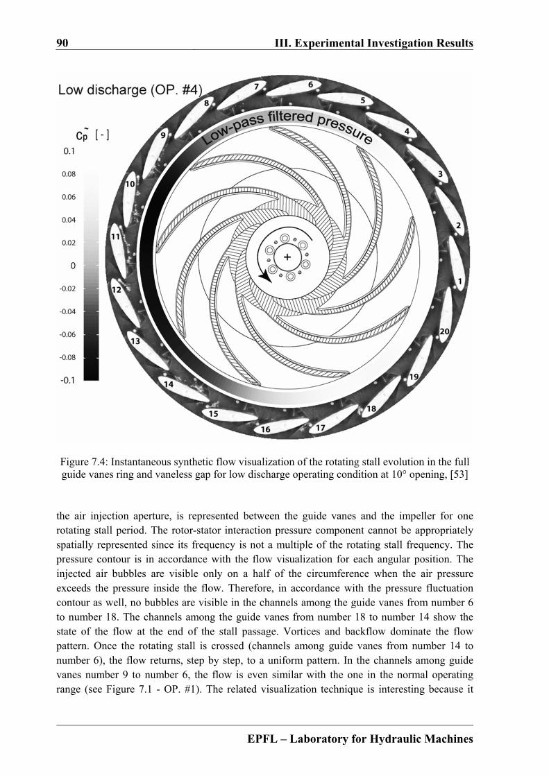
90 III. Experimental Investigation Results
EPFL – Laboratory for Hydraulic Machines
Figure 7.4: Instantaneous synthetic flow visualization of the rotating stall evolution in the full guide vanes ring and vaneless gap for low discharge operating condition at 10° opening, [53]
the air injection aperture, is represented between the guide vanes and the impeller for one rotating stall period. The rotor-stator interaction pressure component cannot be appropriately spatially represented since its frequency is not a multiple of the rotating stall frequency. The pressure contour is in accordance with the flow visualization for each angular position. The injected air bubbles are visible only on a half of the circumference when the air pressure exceeds the pressure inside the flow. Therefore, in accordance with the pressure fluctuation contour as well, no bubbles are visible in the channels among the guide vanes from number 6 to number 18. The channels among the guide vanes from number 18 to number 14 show the state of the flow at the end of the stall passage. Vortices and backflow dominate the flow pattern. Once the rotating stall is crossed (channels among guide vanes from number 14 to number 6), the flow returns, step by step, to a uniform pattern. In the channels among guide vanes number 9 to number 6, the flow is even similar with the one in the normal operating range (see Figure 7.1 - OP. #1). The related visualization technique is interesting because it
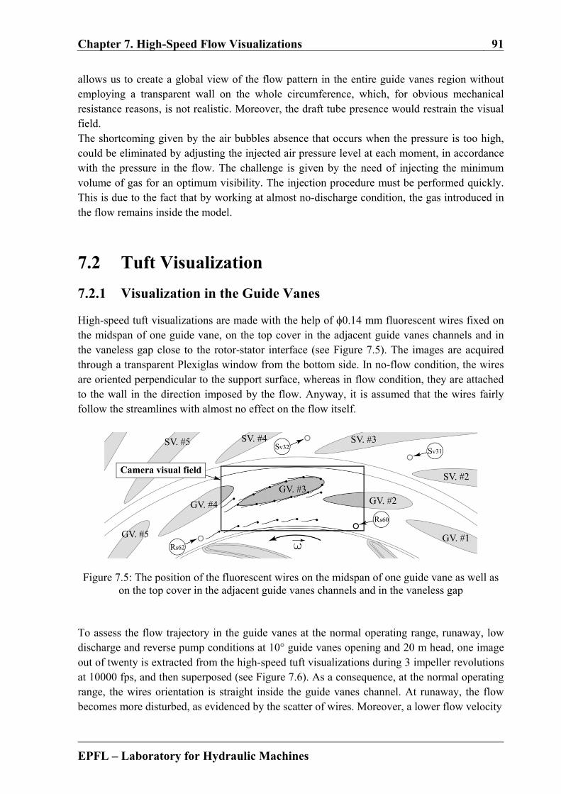
Chapter 7. High-Speed Flow Visualizations 91
EPFL – Laboratory for Hydraulic Machines
allows us to create a global view of the flow pattern in the entire guide vanes region without employing a transparent wall on the whole circumference, which, for obvious mechanical resistance reasons, is not realistic. Moreover, the draft tube presence would restrain the visual field. The shortcoming given by the air bubbles absence that occurs when the pressure is too high, could be eliminated by adjusting the injected air pressure level at each moment, in accordance with the pressure in the flow. The challenge is given by the need of injecting the minimum volume of gas for an optimum visibility. The injection procedure must be performed quickly. This is due to the fact that by working at almost no-discharge condition, the gas introduced in the flow remains inside the model.
7.2 Tuft Visualization
7.2.1 Visualization in the Guide Vanes
High-speed tuft visualizations are made with the help of ϕ0.14 mm fluorescent wires fixed on the midspan of one guide vane, on the top cover in the adjacent guide vanes channels and in the vaneless gap close to the rotor-stator interface (see Figure 7.5). The images are acquired through a transparent Plexiglas window from the bottom side. In no-flow condition, the wires are oriented perpendicular to the support surface, whereas in flow condition, they are attached to the wall in the direction imposed by the flow. Anyway, it is assumed that the wires fairly follow the streamlines with almost no effect on the flow itself.
Figure 7.5: The position of the fluorescent wires on the midspan of one guide vane as well as on the top cover in the adjacent guide vanes channels and in the vaneless gap
To assess the flow trajectory in the guide vanes at the normal operating range, runaway, low discharge and reverse pump conditions at 10° guide vanes opening and 20 m head, one image out of twenty is extracted from the high-speed tuft visualizations during 3 impeller revolutions at 10000 fps, and then superposed (see Figure 7.6). As a consequence, at the normal operating range, the wires orientation is straight inside the guide vanes channel. At runaway, the flow becomes more disturbed, as evidenced by the scatter of wires. Moreover, a lower flow velocity

92 III. Experimental Investigation Results
EPFL – Laboratory for Hydraulic Machines
Figure 7.6: Superposition of tuft visualizations in the guide vanes during 3 impeller revolutions for the normal operating range, runaway, low discharge and reverse pump conditions at 10°
guide vanes opening
Figure 7.7: Superposition of tuft visualizations in the guide vanes during 3 impeller revolutions for the low discharge operating condition at 5°, 10° and 18° guide vanes opening

Chapter 7. High-Speed Flow Visualizations 93
EPFL – Laboratory for Hydraulic Machines
is evidenced by the position of wires on the guide vane suction side. At low discharge and during the passage of the rotating stall, the wire placed in the guide vanes channels suggests the occurrence of backflow. In addition, the history of wires position on the guide vane suction side indicates no-flow condition during the rotating stall passage. To conclude, in reverse pump mode, the wires placed in the guide vanes channel and on the guide vane suction side indicate a pumping mode flow, whilst the wires placed in the vaneless gap between the impeller and the guide vanes and on the guide vane pressure side, are oriented towards the flow in turbine mode. Hence, in such condition, the flow changes its direction between the downstream and the upstream side of the guide vanes, from the turbine to the pumping mode respectively. Figure 7.7 shows the superposition of tuft visualization images captured during 3 impeller revolutions for the low discharge operating condition at 5°, 10° and 18° guide vanes opening. At 5° guide vanes opening the characteristic curve is not positive sloped at runaway and turbine brake mode. Consequently, as mentioned in the previous chapter, no rotating stall development is detected with the pressure fluctuations in the stator. This statement is actually confirmed by the wires at 5° guide vanes opening since their position indicates only the turbine mode flow direction. In contrast, however, at 10° and 18° guide vanes opening the wires position evidences backflow in the guide vanes channels when operating at low positive discharge condition in the positive sloped part of the characteristic. The low discharge condition at 10° guide vanes opening (OP. #4) is now considered. The tuft visualizations are performed along with the pressure measurement at the rotor-stator interface (sensor location Rs62). In Figure 7.10, the original signal of the pressure coefficient fluctuation at the location Rs62 is plotted for one rotating stall period. The low-pass filtered signal related to the rotating stall is also displayed. Then, the low-pass filtered signal at the location Rs61, placed in front of the guide vanes channel captured in the tuft visualizations, is estimated from the signal at the position Rs62, knowing the rotating stall speed and the sensors angular position. For each phase from π/4 to π/4 radians of one rotating stall period, the tuft visualization images are extracted from the whole high-speed recording and then superposed. Finally, from the tuft visualizations in the guide vanes synchronized with the pressure fluctuation during one rotating stall period, in can be observed that, during the pressure increase (0 to π/2 and 3π/2 to 2π phases), the wires position indicates a normal turbine mode flow, whereas during the pressure decrease (phases from π/2 to 3π/2), the wires position suggests the backflow presence in the guide vanes channel.
7.2.2 Visualization at the Impeller Outlet
As illustrated in Figure 7.8, high-speed tuft visualizations, along with the pressure measurements in the stator, are carried out with the help of Φ0.14 mm fluorescent wires fixed on the impeller blades suction side close to the leading edge. The images are acquired through the transparent draft tube cone made of Plexiglas. In no-flow condition, the wires are oriented perpendicular to the support surface, while in flow condition they are attached to the wall in the direction imposed by the flow. Anyway, being placed in the rotating frame, the wires give the direction of the relative velocity .
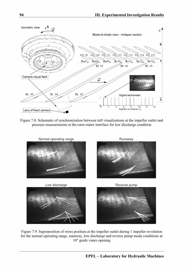
94 III. Experimental Investigation Results
EPFL – Laboratory for Hydraulic Machines
Figure 7.8: Schematic of synchronization between tuft visualizations at the impeller outlet and pressure measurements at the rotor-stator interface for low discharge condition
Figure 7.9: Superposition of wires position at the impeller outlet during 1 impeller revolution for the normal operating range, runaway, low discharge and reverse pump mode conditions at
10° guide vanes opening
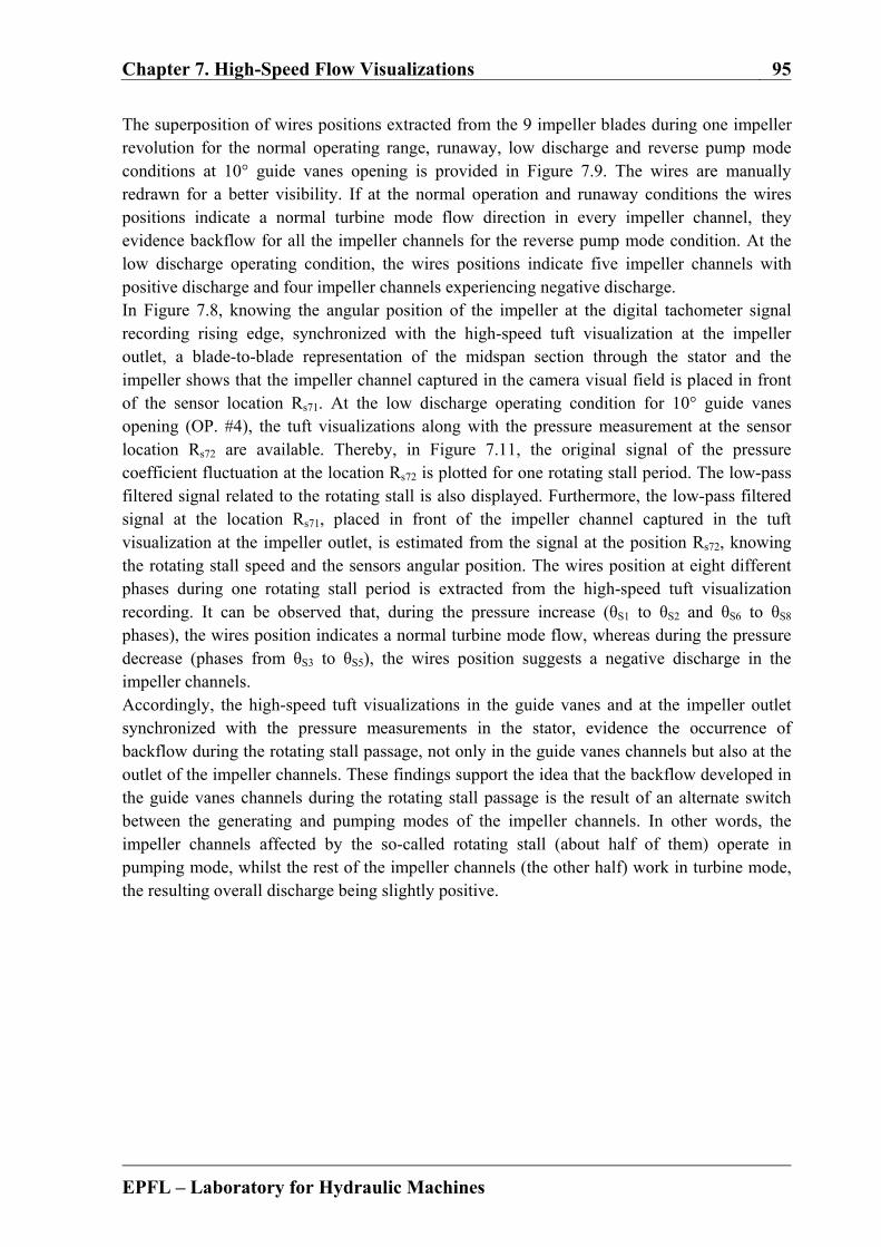
Chapter 7. High-Speed Flow Visualizations 95
EPFL – Laboratory for Hydraulic Machines
The superposition of wires positions extracted from the 9 impeller blades during one impeller revolution for the normal operating range, runaway, low discharge and reverse pump mode conditions at 10° guide vanes opening is provided in Figure 7.9. The wires are manually redrawn for a better visibility. If at the normal operation and runaway conditions the wires positions indicate a normal turbine mode flow direction in every impeller channel, they evidence backflow for all the impeller channels for the reverse pump mode condition. At the low discharge operating condition, the wires positions indicate five impeller channels with positive discharge and four impeller channels experiencing negative discharge. In Figure 7.8, knowing the angular position of the impeller at the digital tachometer signal recording rising edge, synchronized with the high-speed tuft visualization at the impeller outlet, a blade-to-blade representation of the midspan section through the stator and the impeller shows that the impeller channel captured in the camera visual field is placed in front of the sensor location Rs71. At the low discharge operating condition for 10° guide vanes opening (OP. #4), the tuft visualizations along with the pressure measurement at the sensor location Rs72 are available. Thereby, in Figure 7.11, the original signal of the pressure coefficient fluctuation at the location Rs72 is plotted for one rotating stall period. The low-pass filtered signal related to the rotating stall is also displayed. Furthermore, the low-pass filtered signal at the location Rs71, placed in front of the impeller channel captured in the tuft visualization at the impeller outlet, is estimated from the signal at the position Rs72, knowing the rotating stall speed and the sensors angular position. The wires position at eight different phases during one rotating stall period is extracted from the high-speed tuft visualization recording. It can be observed that, during the pressure increase (θS1 to θS2 and θS6 to θS8 phases), the wires position indicates a normal turbine mode flow, whereas during the pressure decrease (phases from θS3 to θS5), the wires position suggests a negative discharge in the impeller channels. Accordingly, the high-speed tuft visualizations in the guide vanes and at the impeller outlet synchronized with the pressure measurements in the stator, evidence the occurrence of backflow during the rotating stall passage, not only in the guide vanes channels but also at the outlet of the impeller channels. These findings support the idea that the backflow developed in the guide vanes channels during the rotating stall passage is the result of an alternate switch between the generating and pumping modes of the impeller channels. In other words, the impeller channels affected by the so-called rotating stall (about half of them) operate in pumping mode, whilst the rest of the impeller channels (the other half) work in turbine mode, the resulting overall discharge being slightly positive.
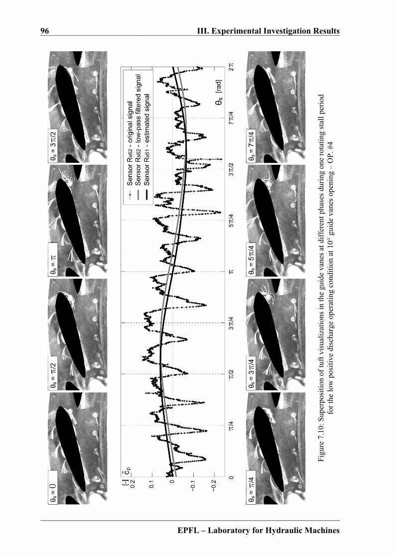
96 III. Experimental Investigation Results
EPFL – Laboratory for Hydraulic Machines
Figu
re 7
.10:
Sup
erpo
siti
on o
f tu
ft v
isua
liza
tions
in th
e gu
ide
vane
s at
dif
fere
nt p
hase
s du
ring
one
rot
atin
g st
all p
erio
d fo
r th
e lo
w p
osit
ive
disc
harg
e op
erat
ing
cond
itio
n at
10°
gui
de v
anes
ope
ning
– O
P. #
4
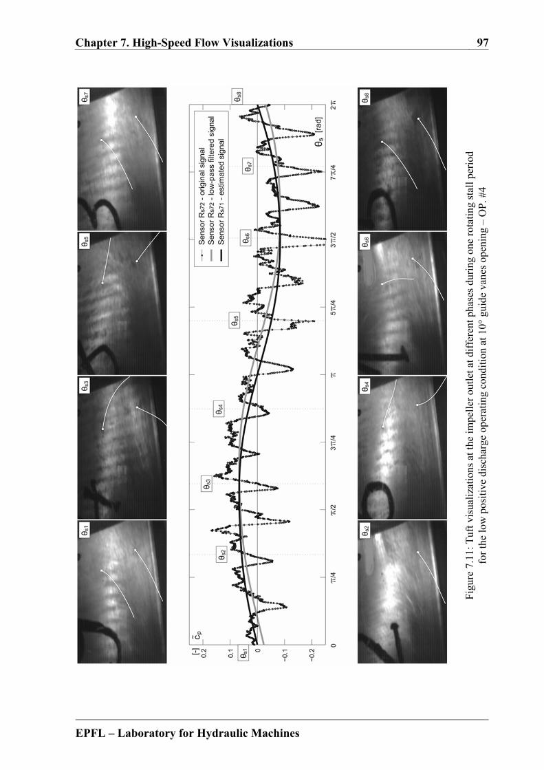
Chapter 7. High-Speed Flow Visualizations 97
EPFL – Laboratory for Hydraulic Machines
Fig
ure
7.11
: Tuf
t vis
uali
zatio
ns a
t the
impe
ller
out
let a
t dif
fere
nt p
hase
s du
ring
one
rot
atin
g st
all p
erio
d fo
r th
e lo
w p
osit
ive
disc
harg
e op
erat
ing
cond
itio
n at
10°
gui
de v
anes
ope
ning
– O
P. #
4

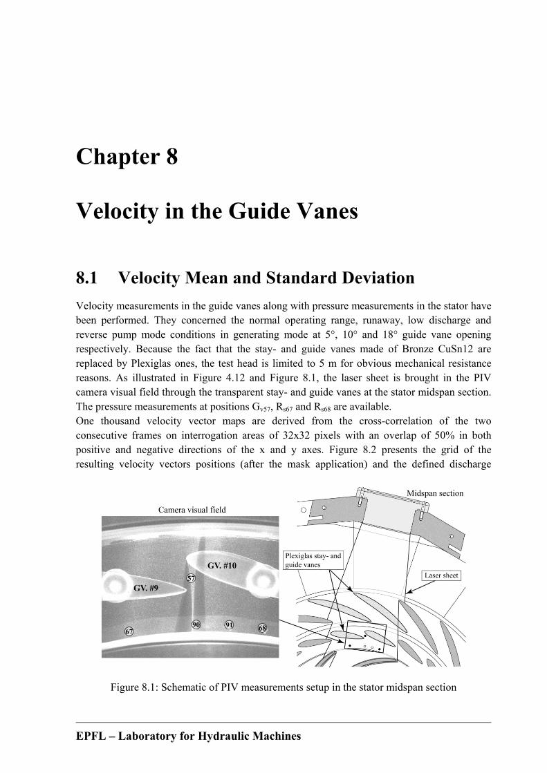
EPFL – Laboratory for Hydraulic Machines
Chapter 8
Velocity in the Guide Vanes
8.1 Velocity Mean and Standard Deviation
Velocity measurements in the guide vanes along with pressure measurements in the stator have been performed. They concerned the normal operating range, runaway, low discharge and reverse pump mode conditions in generating mode at 5°, 10° and 18° guide vane opening respectively. Because the fact that the stay- and guide vanes made of Bronze CuSn12 are replaced by Plexiglas ones, the test head is limited to 5 m for obvious mechanical resistance reasons. As illustrated in Figure 4.12 and Figure 8.1, the laser sheet is brought in the PIV camera visual field through the transparent stay- and guide vanes at the stator midspan section. The pressure measurements at positions Gv57, Rs67 and Rs68 are available. One thousand velocity vector maps are derived from the cross-correlation of the two consecutive frames on interrogation areas of 32x32 pixels with an overlap of 50% in both positive and negative directions of the x and y axes. Figure 8.2 presents the grid of the resulting velocity vectors positions (after the mask application) and the defined discharge
Figure 8.1: Schematic of PIV measurements setup in the stator midspan section
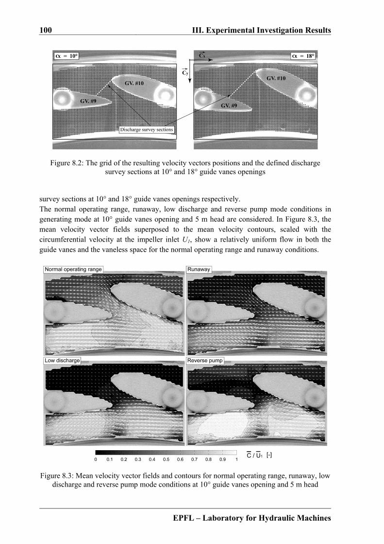
100 III. Experimental Investigation Results
EPFL – Laboratory for Hydraulic Machines
Figure 8.2: The grid of the resulting velocity vectors positions and the defined discharge survey sections at 10° and 18° guide vanes openings
survey sections at 10° and 18° guide vanes openings respectively. The normal operating range, runaway, low discharge and reverse pump mode conditions in generating mode at 10° guide vanes opening and 5 m head are considered. In Figure 8.3, the mean velocity vector fields superposed to the mean velocity contours, scaled with the circumferential velocity at the impeller inlet U1, show a relatively uniform flow in both the guide vanes and the vaneless space for the normal operating range and runaway conditions.
Figure 8.3: Mean velocity vector fields and contours for normal operating range, runaway, low discharge and reverse pump mode conditions at 10° guide vanes opening and 5 m head
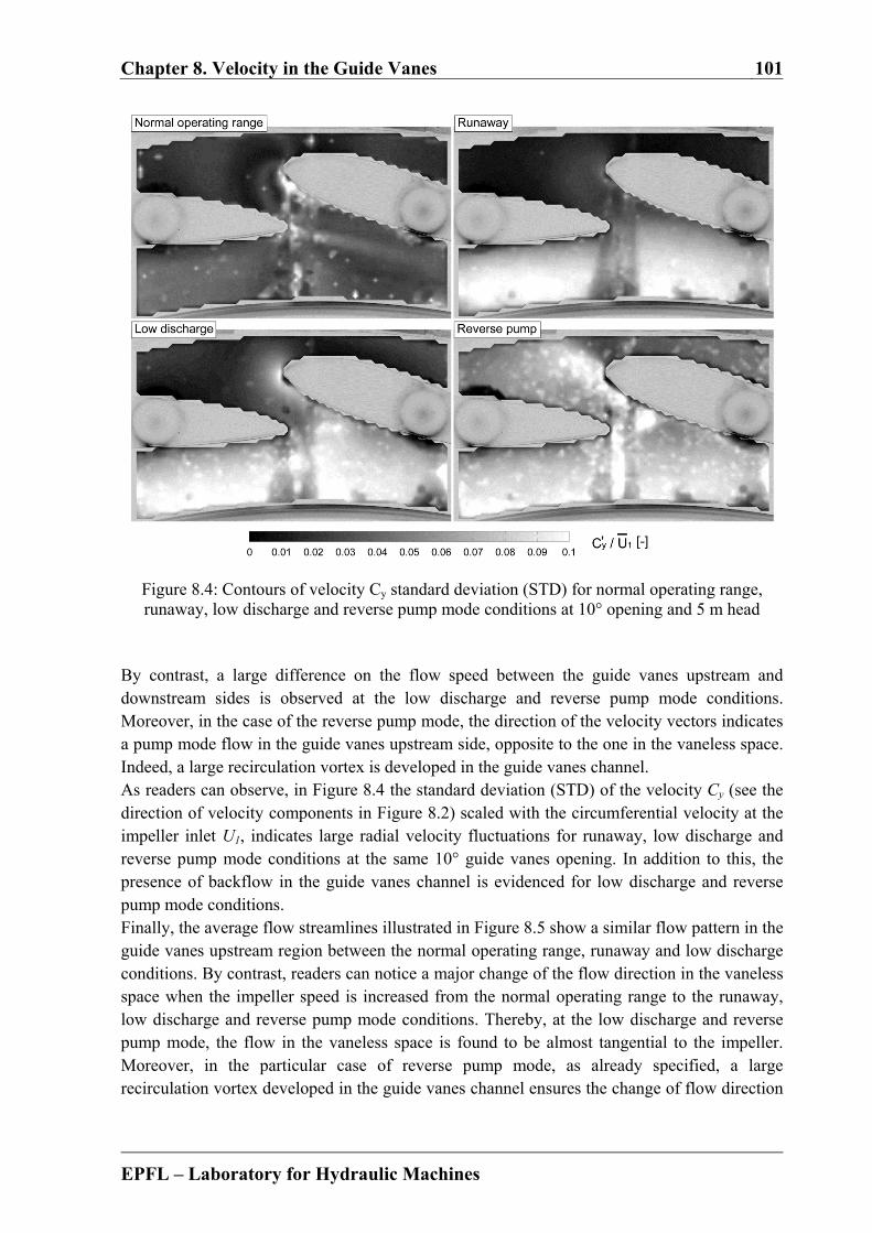
Chapter 8. Velocity in the Guide Vanes 101
EPFL – Laboratory for Hydraulic Machines
Figure 8.4: Contours of velocity Cy standard deviation (STD) for normal operating range, runaway, low discharge and reverse pump mode conditions at 10° opening and 5 m head
By contrast, a large difference on the flow speed between the guide vanes upstream and downstream sides is observed at the low discharge and reverse pump mode conditions. Moreover, in the case of the reverse pump mode, the direction of the velocity vectors indicates a pump mode flow in the guide vanes upstream side, opposite to the one in the vaneless space. Indeed, a large recirculation vortex is developed in the guide vanes channel. As readers can observe, in Figure 8.4 the standard deviation (STD) of the velocity Cy (see the direction of velocity components in Figure 8.2) scaled with the circumferential velocity at the impeller inlet U1, indicates large radial velocity fluctuations for runaway, low discharge and reverse pump mode conditions at the same 10° guide vanes opening. In addition to this, the presence of backflow in the guide vanes channel is evidenced for low discharge and reverse pump mode conditions. Finally, the average flow streamlines illustrated in Figure 8.5 show a similar flow pattern in the guide vanes upstream region between the normal operating range, runaway and low discharge conditions. By contrast, readers can notice a major change of the flow direction in the vaneless space when the impeller speed is increased from the normal operating range to the runaway, low discharge and reverse pump mode conditions. Thereby, at the low discharge and reverse pump mode, the flow in the vaneless space is found to be almost tangential to the impeller. Moreover, in the particular case of reverse pump mode, as already specified, a large recirculation vortex developed in the guide vanes channel ensures the change of flow direction
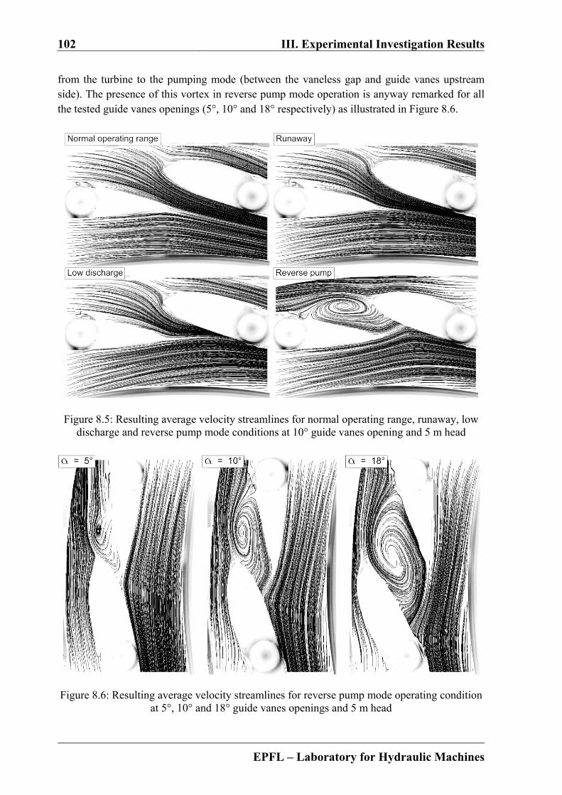
102 III. Experimental Investigation Results
EPFL – Laboratory for Hydraulic Machines
from the turbine to the pumping mode (between the vaneless gap and guide vanes upstream side). The presence of this vortex in reverse pump mode operation is anyway remarked for all the tested guide vanes openings (5°, 10° and 18° respectively) as illustrated in Figure 8.6.
Figure 8.5: Resulting average velocity streamlines for normal operating range, runaway, low discharge and reverse pump mode conditions at 10° guide vanes opening and 5 m head
Figure 8.6: Resulting average velocity streamlines for reverse pump mode operating condition at 5°, 10° and 18° guide vanes openings and 5 m head

Chapter 8. Velocity in the Guide Vanes 103
EPFL – Laboratory for Hydraulic Machines
Figure 8.7: Mean velocity vector fields and contours for low discharge operating condition at 5°, 10° and 18° guide vanes openings and 5 m head
Figure 8.8: The contours of velocity Cy standard deviation (STD) for low discharge operating condition at 5°, 10° and 18° guide vanes openings and 5 m head
Considering the low discharge operating condition at 5 m head, the magnitude of the absolute mean velocity fields, divided to the circumferential velocity at the impeller inlet U1, decreases as the guide vanes opening angle from 5° to 10° and 18° increase (see Figure 8.7). The standard deviation of the velocity Cy, scaled with the circumferential velocity at the impeller inlet U1, indicates in Figure 8.8, the presence of backflow in the guide vanes channel only for 10° and 18° guide vanes openings. This is also confirmed by the pressure measurements in the stator, since any rotating stall is detected at 5° guide vanes opening angle when operating in

104 III. Experimental Investigation Results
EPFL – Laboratory for Hydraulic Machines
the S-region of the characteristic. To conclude, from the average flow streamlines illustrated in Figure 8.9, readers should notice that the stagnation point moves on the guide vane pressure side toward the leading edge with the opening increasing from 5° to 10° and to 18°.
Figure 8.9: Resulting average velocity streamlines for low discharge operating condition at 5°, 10° and 18° guide vanes openings and 5 m head
8.2 Fluctuations during the Stall Passage
One thousand velocity fields are acquired at a time interval TPIV = 0.75 s longer than the rotating stall rotational period. Thereby, to reconstruct the flow field evolution during one rotating stall passage, the velocity vectors must be arranged according to the rotating stall phase. The low discharge operating condition at 10° guide vanes opening and 5 m head is first considered. The pressure fluctuation at the rotor-stator interface (sensor location Rs90 – see Figure 8.1), recorded along with the PIV measurements, is used to compute the rotating stall instantaneous phase of the PIV visual field by employing the method described in Section 6.2.1 - Pressure Fluctuations into the Stator. Then, as illustrated in Figure 8.10, the photodiode signal, which gives the PIV acquisition trigger, is used to recover the rotating stall instantaneous phase associated to every PIV capture along with the values of the original and the low-pass filtered pressure at the Rs90 location. In the next step, a guide vanes channel discharge coefficient is computed on the already defined survey section (see Figure 8.2) by adopting the procedure explained in the following lines.
Knowing the velocity and the surface normal , the discharge Q of a surface S is:
S
Q C n dS (8.1)
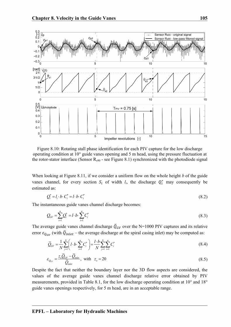
Chapter 8. Velocity in the Guide Vanes 105
EPFL – Laboratory for Hydraulic Machines
Figure 8.10: Rotating stall phase identification for each PIV capture for the low discharge operating condition at 10° guide vanes opening and 5 m head, using the pressure fluctuation at the rotor-stator interface (Sensor Rs90 - see Figure 8.1) synchronized with the photodiode signal
When looking at Figure 8.11, if we consider a uniform flow on the whole height b of the guide vanes channel, for every section of width li, the discharge ∗ may consequently be estimated as:
* * *i i i iQ l b C l b C (8.2)
The instantaneous guide vanes channel discharge becomes:
* *
1 1
n n
GV i ii i
Q Q l b C
(8.3)
The average guide vanes channel discharge over the N=1000 PIV captures and its relative error (with – the average discharge at the spiral casing inlet) may be computed as:
* *
1 1 1 1
1 N n N n
GV i ij i j i
l bQ l b C C
N N
(8.4)
, with 20GV
o GV inletQ o
inlet
z Q Qz
Q
(8.5)
Despite the fact that neither the boundary layer nor the 3D flow aspects are considered, the values of the average guide vanes channel discharge relative error obtained by PIV measurements, provided in Table 8.1, for the low discharge operating condition at 10° and 18° guide vanes openings respectively, for 5 m head, are in an acceptable range.
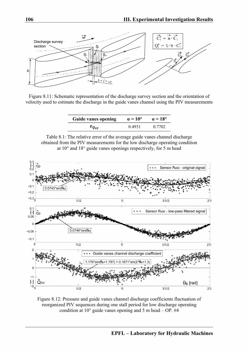
106 III. Experimental Investigation Results
EPFL – Laboratory for Hydraulic Machines
Figure 8.11: Schematic representation of the discharge survey section and the orientation of velocity used to estimate the discharge in the guide vanes channel using the PIV measurements
Guide vanes opening α = 10° α = 18°
0.4931 0.7702
Table 8.1: The relative error of the average guide vanes channel discharge obtained from the PIV measurements for the low discharge operating condition
at 10° and 18° guide vanes openings respectively, for 5 m head
Figure 8.12: Pressure and guide vanes channel discharge coefficients fluctuation of reorganized PIV sequences during one stall period for low discharge operating
condition at 10° guide vanes opening and 5 m head – OP. #4

Chapter 8. Velocity in the Guide Vanes 107
EPFL – Laboratory for Hydraulic Machines
The guide vanes channel discharge coefficient is obtained from the following relation:
* * * *
1 1 1 1 1 1
* *
1 1 1 1
1
1
n N n n N n
i i i ii j i i j iGV GV
GV N n N nGV
i ij i j i
l bl b C C C C
N NQ QQ
l bQ C CN N
(8.6)
Finally, the one thousand velocity fields are arranged by the rotating stall instantaneous phase in ascending order over one period (θS = 0÷2π). The same procedure is however repeated for the low discharge operating condition at 18° guide vanes opening and 5 m head case. Thereby, Figure 8.12 and Figure 8.13 respectively, provide the synchronized fluctuation of pressure and guide vanes channel discharge coefficients, during one rotating stall period, for the low discharge condition at 10° and 18° guide vanes openings, resulting from the reorganized PIV sequences. In both 10° and 18° opening cases, a phase shift of about π/2 between the guide vanes channel discharge and pressure fluctuations, during the rotating stall passage, is noticed. Indeed, this finding confirms the hydrodynamics of the rotating stall passage in the guide vanes observed with the high-speed visualizations: the increase of pressure in the guide vanes channels is associated with a flow in normal turbine way, the channels being overloaded, while the decrease of pressure is combined with a reduced and even with a negative discharge, the flow structure being similar to the one in reverse pump mode.
Figure 8.13: Pressure and guide vanes channel discharge coefficients fluctuation of reorganized PIV sequences during one stall period for low discharge operating
condition at 18° guide vanes opening and 5 m head
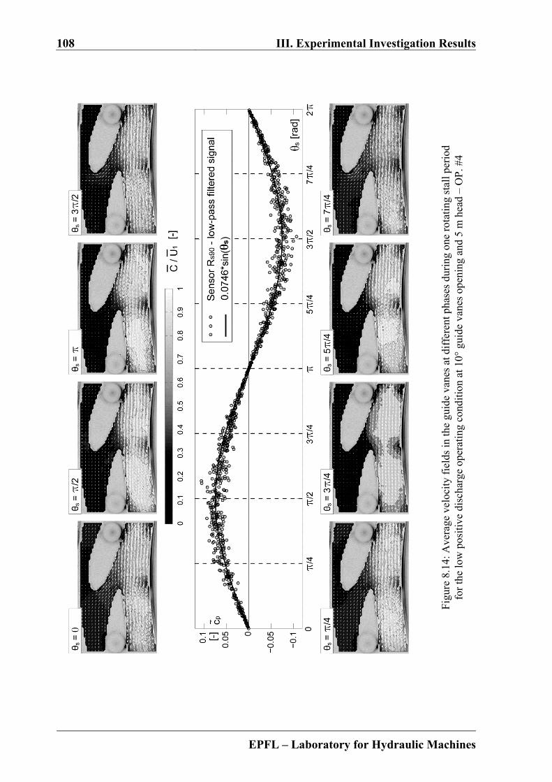
108 III. Experimental Investigation Results
EPFL – Laboratory for Hydraulic Machines
Fig
ure
8.14
: Ave
rage
vel
ocit
y fi
elds
in th
e gu
ide
vane
s at
dif
fere
nt p
hase
s du
ring
one
rot
atin
g st
all p
erio
d fo
r th
e lo
w p
osit
ive
disc
harg
e op
erat
ing
cond
itio
n at
10°
gui
de v
anes
ope
ning
and
5 m
hea
d –
OP
. #4
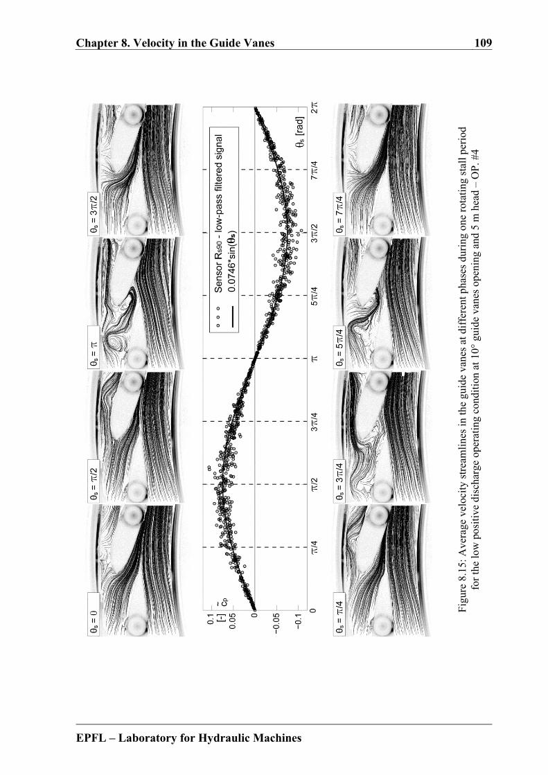
Chapter 8. Velocity in the Guide Vanes 109
EPFL – Laboratory for Hydraulic Machines
Fig
ure
8.15
: Ave
rage
vel
ocit
y st
ream
line
s in
the
guid
e va
nes
at d
iffe
rent
pha
ses
duri
ng o
ne r
otat
ing
stal
l per
iod
for
the
low
pos
itiv
e di
scha
rge
oper
atin
g co
ndit
ion
at 1
0° g
uide
van
es o
peni
ng a
nd 5
m h
ead
– O
P. #
4
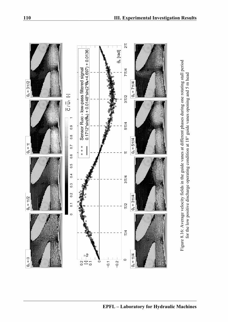
110 III. Experimental Investigation Results
EPFL – Laboratory for Hydraulic Machines
Fig
ure
8.16
: Ave
rage
vel
ocit
y fi
elds
in th
e gu
ide
vane
s at
dif
fere
nt p
hase
s du
ring
one
rot
atin
g st
all p
erio
d fo
r th
e lo
w p
osit
ive
disc
harg
e op
erat
ing
cond
itio
n at
18°
gui
de v
anes
ope
ning
and
5 m
hea
d

Chapter 8. Velocity in the Guide Vanes 111
EPFL – Laboratory for Hydraulic Machines
Fig
ure
8.17
: Ave
rage
vel
ocit
y st
ream
line
s in
the
guid
e va
nes
at d
iffe
rent
pha
ses
duri
ng o
ne r
otat
ing
stal
l per
iod
for
the
low
pos
itive
dis
char
ge o
pera
ting
cond
itio
n at
18°
gui
de v
anes
ope
ning
and
5 m
hea
d
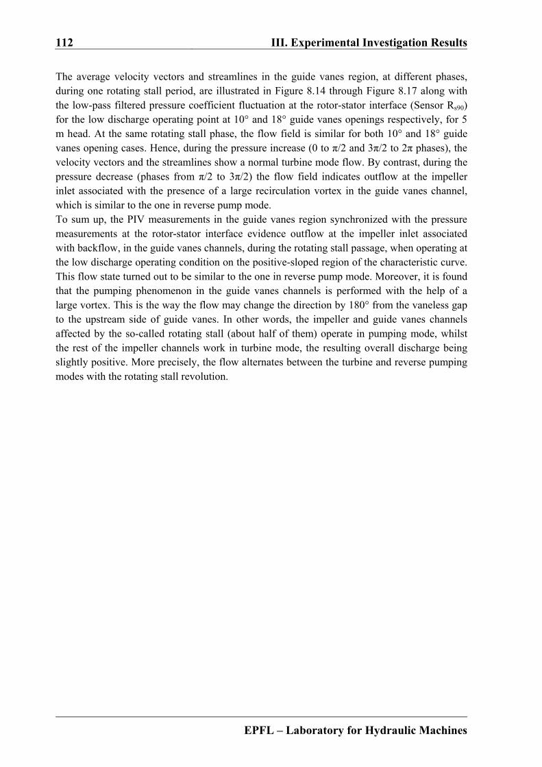
112 III. Experimental Investigation Results
EPFL – Laboratory for Hydraulic Machines
The average velocity vectors and streamlines in the guide vanes region, at different phases, during one rotating stall period, are illustrated in Figure 8.14 through Figure 8.17 along with the low-pass filtered pressure coefficient fluctuation at the rotor-stator interface (Sensor Rs90) for the low discharge operating point at 10° and 18° guide vanes openings respectively, for 5 m head. At the same rotating stall phase, the flow field is similar for both 10° and 18° guide vanes opening cases. Hence, during the pressure increase (0 to π/2 and 3π/2 to 2π phases), the velocity vectors and the streamlines show a normal turbine mode flow. By contrast, during the pressure decrease (phases from π/2 to 3π/2) the flow field indicates outflow at the impeller inlet associated with the presence of a large recirculation vortex in the guide vanes channel, which is similar to the one in reverse pump mode. To sum up, the PIV measurements in the guide vanes region synchronized with the pressure measurements at the rotor-stator interface evidence outflow at the impeller inlet associated with backflow, in the guide vanes channels, during the rotating stall passage, when operating at the low discharge operating condition on the positive-sloped region of the characteristic curve. This flow state turned out to be similar to the one in reverse pump mode. Moreover, it is found that the pumping phenomenon in the guide vanes channels is performed with the help of a large vortex. This is the way the flow may change the direction by 180° from the vaneless gap to the upstream side of guide vanes. In other words, the impeller and guide vanes channels affected by the so-called rotating stall (about half of them) operate in pumping mode, whilst the rest of the impeller channels work in turbine mode, the resulting overall discharge being slightly positive. More precisely, the flow alternates between the turbine and reverse pumping modes with the rotating stall revolution.

EPFL – Laboratory for Hydraulic Machines
Part IV
Numerical Investigation Results

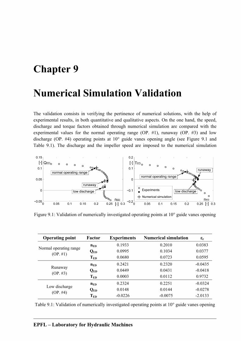
EPFL – Laboratory for Hydraulic Machines
Chapter 9
Numerical Simulation Validation
The validation consists in verifying the pertinence of numerical solutions, with the help of experimental results, in both quantitative and qualitative aspects. On the one hand, the speed, discharge and torque factors obtained through numerical simulation are compared with the experimental values for the normal operating range (OP. #1), runaway (OP. #3) and low discharge (OP. #4) operating points at 10° guide vanes opening angle (see Figure 9.1 and Table 9.1). The discharge and the impeller speed are imposed to the numerical simulation
Figure 9.1: Validation of numerically investigated operating points at 10° guide vanes opening
Operating point Factor Experiments Numerical simulation εr
Normal operating range (OP. #1)
nED 0.1933 0.2010 0.0383
QED 0.0995 0.1034 0.0377
TED 0.0680 0.0723 0.0595
Runaway (OP. #3)
nED 0.2421 0.2320 -0.0435
QED 0.0449 0.0431 -0.0418
TED 0.0003 0.0112 0.9732
Low discharge (OP. #4)
nED 0.2324 0.2251 -0.0324
QED 0.0148 0.0144 -0.0278
TED -0.0226 -0.0075 -2.0133
Table 9.1: Validation of numerically investigated operating points at 10° guide vanes opening
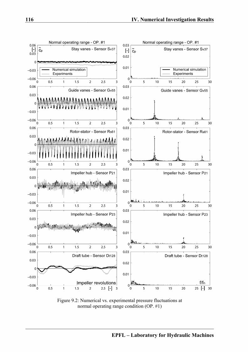
116 IV. Numerical Investigation Results
EPFL – Laboratory for Hydraulic Machines
Figure 9.2: Numerical vs. experimental pressure fluctuations at normal operating range condition (OP. #1)
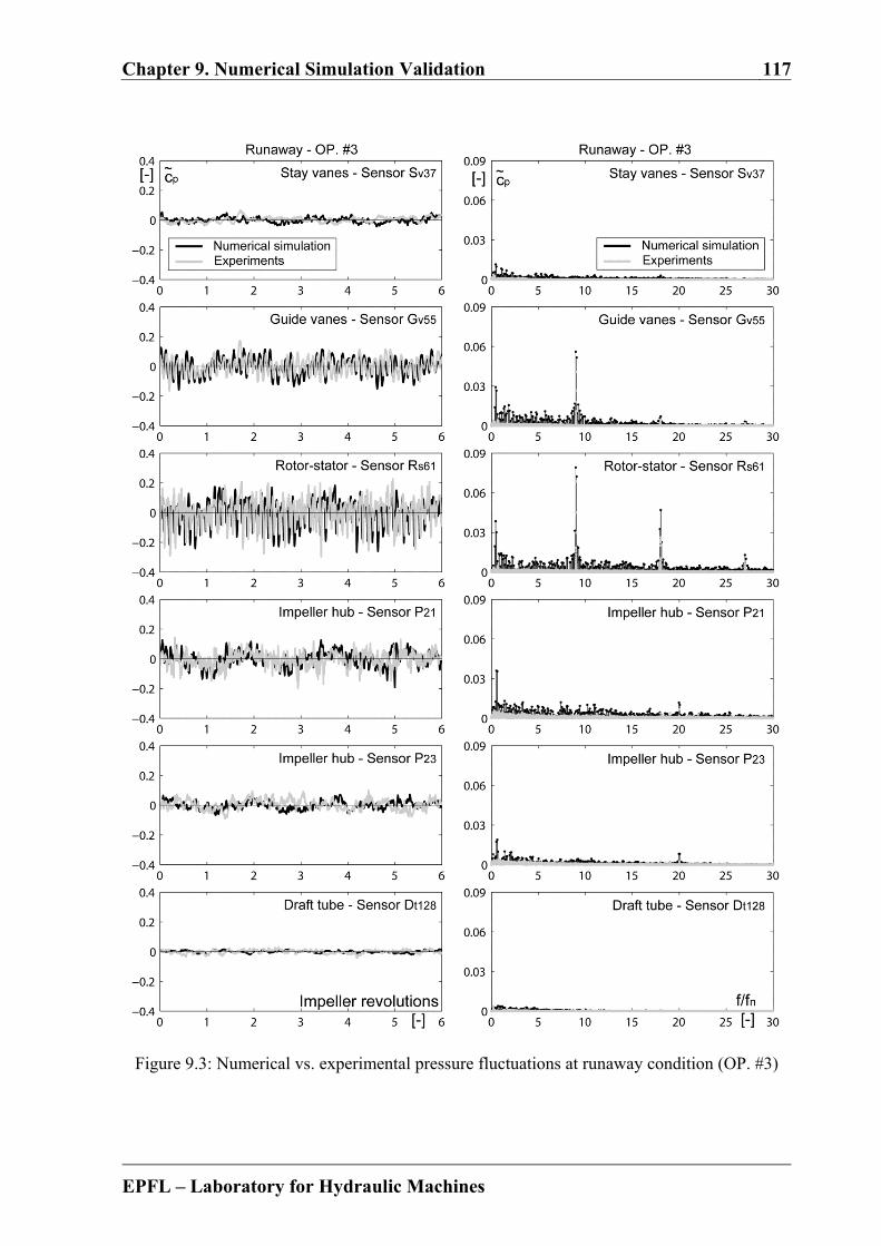
Chapter 9. Numerical Simulation Validation 117
EPFL – Laboratory for Hydraulic Machines
Figure 9.3: Numerical vs. experimental pressure fluctuations at runaway condition (OP. #3)
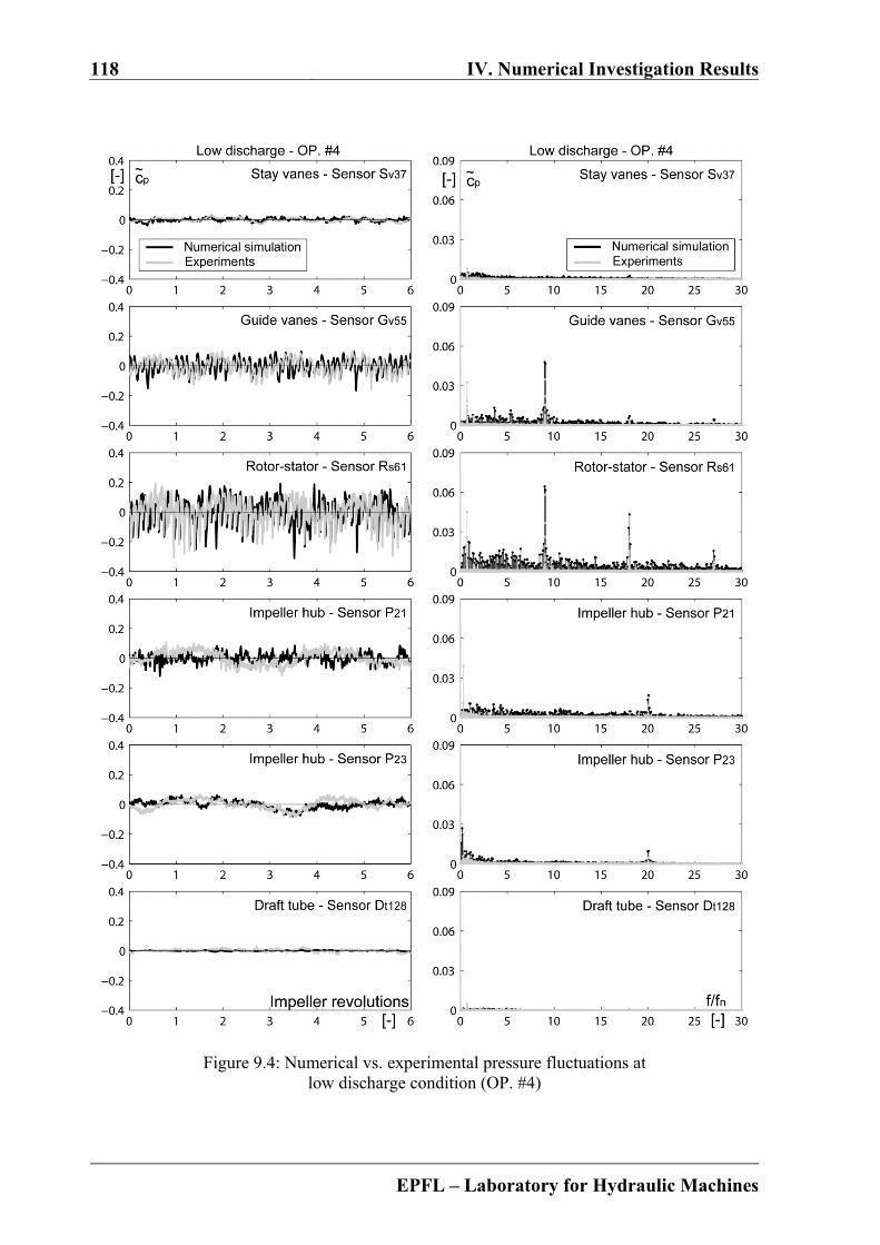
118 IV. Numerical Investigation Results
EPFL – Laboratory for Hydraulic Machines
Figure 9.4: Numerical vs. experimental pressure fluctuations at low discharge condition (OP. #4)
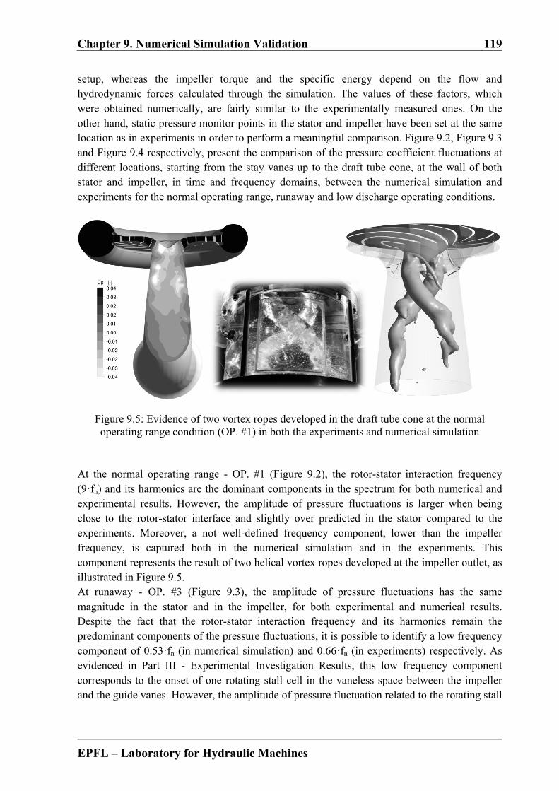
Chapter 9. Numerical Simulation Validation 119
EPFL – Laboratory for Hydraulic Machines
setup, whereas the impeller torque and the specific energy depend on the flow and hydrodynamic forces calculated through the simulation. The values of these factors, which were obtained numerically, are fairly similar to the experimentally measured ones. On the other hand, static pressure monitor points in the stator and impeller have been set at the same location as in experiments in order to perform a meaningful comparison. Figure 9.2, Figure 9.3 and Figure 9.4 respectively, present the comparison of the pressure coefficient fluctuations at different locations, starting from the stay vanes up to the draft tube cone, at the wall of both stator and impeller, in time and frequency domains, between the numerical simulation and experiments for the normal operating range, runaway and low discharge operating conditions.
Figure 9.5: Evidence of two vortex ropes developed in the draft tube cone at the normal operating range condition (OP. #1) in both the experiments and numerical simulation
At the normal operating range - OP. #1 (Figure 9.2), the rotor-stator interaction frequency (9·fn) and its harmonics are the dominant components in the spectrum for both numerical and experimental results. However, the amplitude of pressure fluctuations is larger when being close to the rotor-stator interface and slightly over predicted in the stator compared to the experiments. Moreover, a not well-defined frequency component, lower than the impeller frequency, is captured both in the numerical simulation and in the experiments. This component represents the result of two helical vortex ropes developed at the impeller outlet, as illustrated in Figure 9.5. At runaway - OP. #3 (Figure 9.3), the amplitude of pressure fluctuations has the same magnitude in the stator and in the impeller, for both experimental and numerical results. Despite the fact that the rotor-stator interaction frequency and its harmonics remain the predominant components of the pressure fluctuations, it is possible to identify a low frequency component of 0.53·fn (in numerical simulation) and 0.66·fn (in experiments) respectively. As evidenced in Part III - Experimental Investigation Results, this low frequency component corresponds to the onset of one rotating stall cell in the vaneless space between the impeller and the guide vanes. However, the amplitude of pressure fluctuation related to the rotating stall
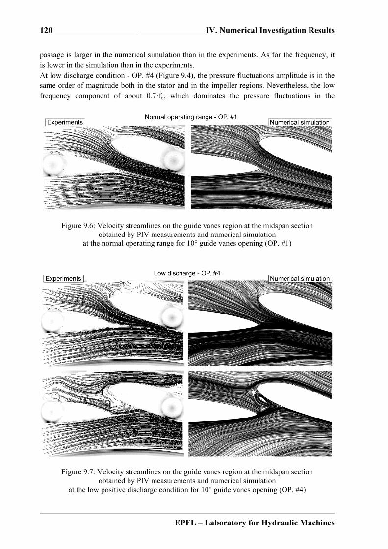
120 IV. Numerical Investigation Results
EPFL – Laboratory for Hydraulic Machines
passage is larger in the numerical simulation than in the experiments. As for the frequency, it is lower in the simulation than in the experiments. At low discharge condition - OP. #4 (Figure 9.4), the pressure fluctuations amplitude is in the same order of magnitude both in the stator and in the impeller regions. Nevertheless, the low frequency component of about 0.7·fn, which dominates the pressure fluctuations in the
Figure 9.6: Velocity streamlines on the guide vanes region at the midspan section obtained by PIV measurements and numerical simulation
at the normal operating range for 10° guide vanes opening (OP. #1)
Figure 9.7: Velocity streamlines on the guide vanes region at the midspan section obtained by PIV measurements and numerical simulation
at the low positive discharge condition for 10° guide vanes opening (OP. #4)

Chapter 9. Numerical Simulation Validation 121
EPFL – Laboratory for Hydraulic Machines
experiments, is not well defined in the numerical simulation. What should be noticed is that, even simulating a very unstable operating point as the low discharge condition, the pressure fluctuations fit relatively well the ones obtained in the experimental investigation although the low frequency component is not precisely predicted. In fact, the operating condition created in the numerical simulation seems similar to the zero discharge condition, where the rotating stall disappears in the experiments. Finally, the PIV measurements are used to qualitatively validate the flow pattern in the guide vanes region obtained by numerical simulation. Thereby, as appears in Figure 9.6, the velocity streamlines on the guide vanes region at the midspan section obtained by numerical simulation, at the normal operating range condition (OP. #1), fit well the ones obtained by PIV measurements. At the low discharge condition (OP. #4), for an overloaded (top) and a blocked (bottom) guide vanes channel, the velocity streamlines illustrated in Figure 9.7 fit relatively well between the PIV measurements and the numerical simulation. Nevertheless, if, in experiments half of the guide vanes circumference operate in turbine mode and the other half in reverse pump mode, the channels affected by backflow are not consecutive although they are mixed with the ones operating in normal turbine way. This is due to the fact that the rotating stall is not well organized in the numerical simulation. To conclude, the onset of the rotating stall phenomenon is experimentally found at runaway and is fully developed toward zero discharge operating condition. However, this phenomenon is not accurately caught at low discharge condition in the numerical simulation. The differences between the numerical and the experimental results found in the pressure may be explained through the presence of major flow separations, especially in the impeller, which is difficult to be simulated with RANS or hybrid RANS-LES methods. Nevertheless, from a qualitative perspective, the numerical simulation results provide readers with important information about the description of the flow pattern under off-design circumstances, in which flow separation that occurs in the impeller channels and vaneless gap between the impeller and the guide vanes, leads to the development of one rotating stall.

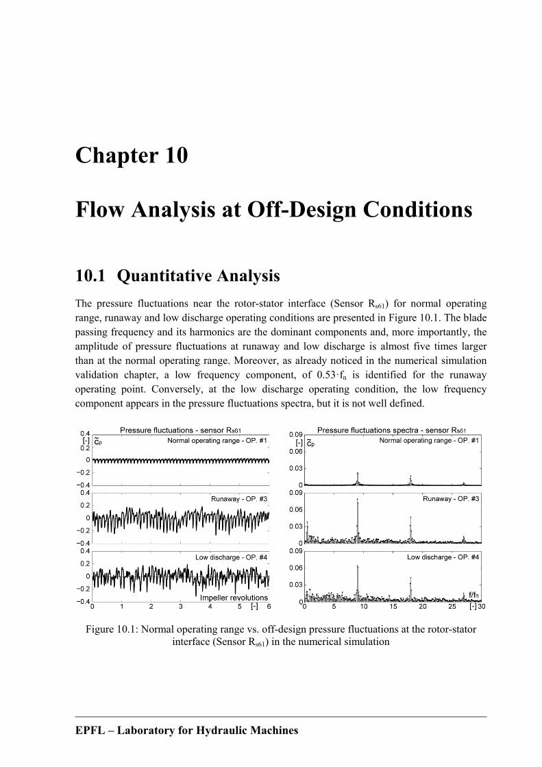
EPFL – Laboratory for Hydraulic Machines
Chapter 10
Flow Analysis at Off-Design Conditions
10.1 Quantitative Analysis
The pressure fluctuations near the rotor-stator interface (Sensor Rs61) for normal operating range, runaway and low discharge operating conditions are presented in Figure 10.1. The blade passing frequency and its harmonics are the dominant components and, more importantly, the amplitude of pressure fluctuations at runaway and low discharge is almost five times larger than at the normal operating range. Moreover, as already noticed in the numerical simulation validation chapter, a low frequency component, of 0.53·fn is identified for the runaway operating point. Conversely, at the low discharge operating condition, the low frequency component appears in the pressure fluctuations spectra, but it is not well defined.
Figure 10.1: Normal operating range vs. off-design pressure fluctuations at the rotor-stator interface (Sensor Rs61) in the numerical simulation
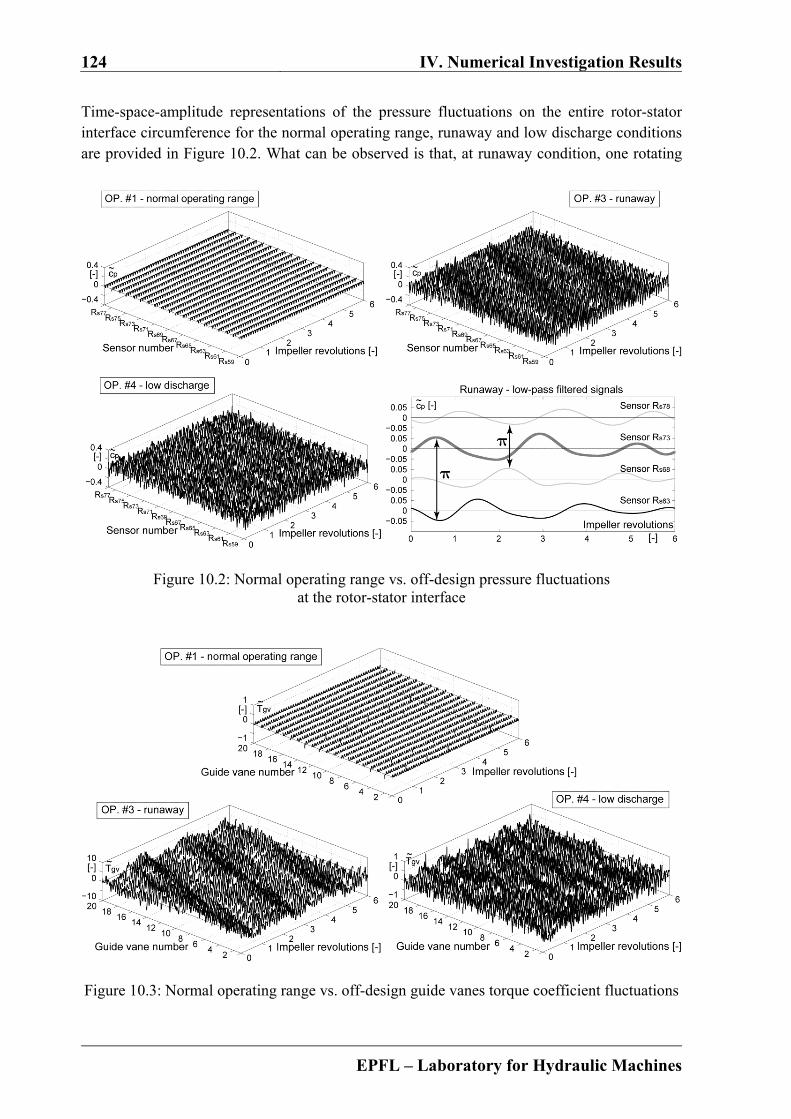
124 IV. Numerical Investigation Results
EPFL – Laboratory for Hydraulic Machines
Time-space-amplitude representations of the pressure fluctuations on the entire rotor-stator interface circumference for the normal operating range, runaway and low discharge conditions are provided in Figure 10.2. What can be observed is that, at runaway condition, one rotating
Figure 10.2: Normal operating range vs. off-design pressure fluctuations at the rotor-stator interface
Figure 10.3: Normal operating range vs. off-design guide vanes torque coefficient fluctuations

Chapter 10. Flow Analysis at Off-Design Conditions 125
EPFL – Laboratory for Hydraulic Machines
stall cell travels with the impeller at subsynchronous speed (0.53·fn) and induces the same fluctuation amplitude in the whole vaneless ring. Moreover, the counter phase fluctuation of the low-pass filtered pressure, for two diametrically opposed positions on the rotor-stator interface, evidences the rotation of one stall source (see the bottom right plot in Figure 10.2). However, at the low discharge condition, no organized rotating stall can be identified from the pressure fluctuations in the vaneless gap between the impeller and the guide vanes.
1
, with 20o
o gv gv
gv oz
gvii
z T TT z
T
(10.1)
In Figure 10.3, at runaway, the amplitude of the guide vanes torque coefficient fluctuation (equation (10.1)) is found to be about 100 times larger than at the normal operating range, and about 10 times larger than at low discharge condition. In addition, the development of the rotating stall phenomenon at runaway condition is also visible in the guide vanes torque fluctuation. Discharge survey sections are defined in the impeller channels as illustrated in the upper right side of Figure 10.4. Time history of the relative discharge in the impeller channels, computed with equation (10.2), reveals fluctuations amplitude that are 20 times larger at runaway and low discharge than at the normal operating range condition (see Figure 10.4). Furthermore, the same plots show the development of the rotating stall at runaway.
, with 9b ich inletich b
inlet
z Q QQ z
Q
(10.2)
Figure 10.4: Normal operating range vs. off-design discharge fluctuations in the impeller channels

126 IV. Numerical Investigation Results
EPFL – Laboratory for Hydraulic Machines
At any moment, half of the impeller channels exhibits a larger discharge than the average, whereas the remaining ones are partially blocked. It must be mentioned that, in the rotating frame, the stall cell rotates at about 47% of the impeller speed. In Figure 10.5, the amplitude of the impeller blades torque coefficient fluctuation (equation (10.3)) is found to be about 50 times larger at off-design than at the normal operating range condition. Moreover, if the rotor-stator interaction frequency (20·fn) is easily visible for each case, no low frequency component related to the presence of the rotating stall can be observed. However, this may come from the fact that the hydrodynamic forces, thus the torque, are not well predicted with the SAS-SST turbulence model when the flow separation phenomenon occurs.
1
, with 9b
b b b
b bz
bii
z T TT z
T
(10.3)
Figure 10.5: Normal operating range vs. off-design impeller blades torque coefficient fluctuations
To sum up, the quantitative analysis of the numerical simulation results shows that the pressure fluctuations in the vaneless space between the impeller and the guide vanes as well as the discharge fluctuations in the impeller channels are much more important at off-design condition compared to the normal operating range. Moreover, at runaway the development of a subsynchronous rotating stall is detected in the guide vanes and in the impeller channels. By contrast, at the low discharge condition, the rotating stall development is not well predicted.
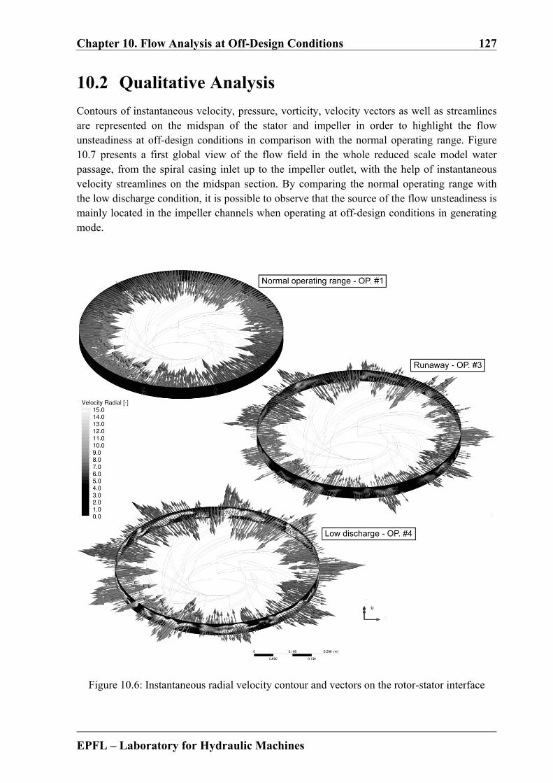
Chapter 10. Flow Analysis at Off-Design Conditions 127
EPFL – Laboratory for Hydraulic Machines
10.2 Qualitative Analysis
Contours of instantaneous velocity, pressure, vorticity, velocity vectors as well as streamlines are represented on the midspan of the stator and impeller in order to highlight the flow unsteadiness at off-design conditions in comparison with the normal operating range. Figure 10.7 presents a first global view of the flow field in the whole reduced scale model water passage, from the spiral casing inlet up to the impeller outlet, with the help of instantaneous velocity streamlines on the midspan section. By comparing the normal operating range with the low discharge condition, it is possible to observe that the source of the flow unsteadiness is mainly located in the impeller channels when operating at off-design conditions in generating mode.
Figure 10.6: Instantaneous radial velocity contour and vectors on the rotor-stator interface
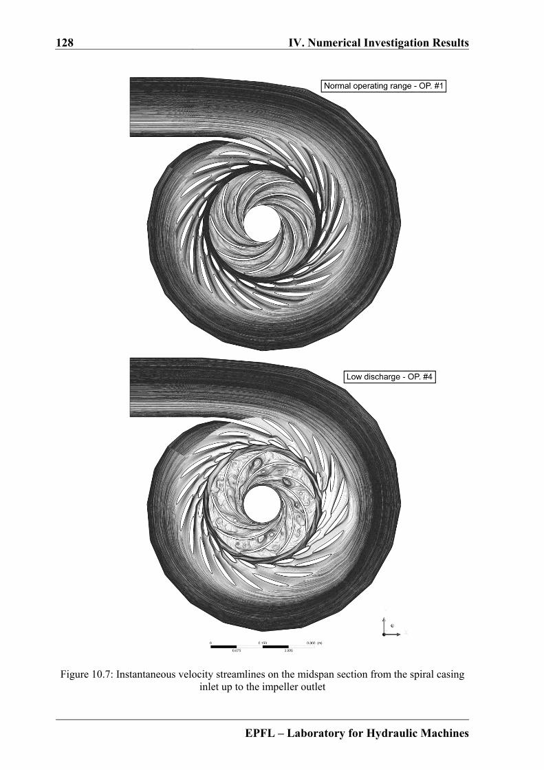
128 IV. Numerical Investigation Results
EPFL – Laboratory for Hydraulic Machines
Figure 10.7: Instantaneous velocity streamlines on the midspan section from the spiral casing inlet up to the impeller outlet
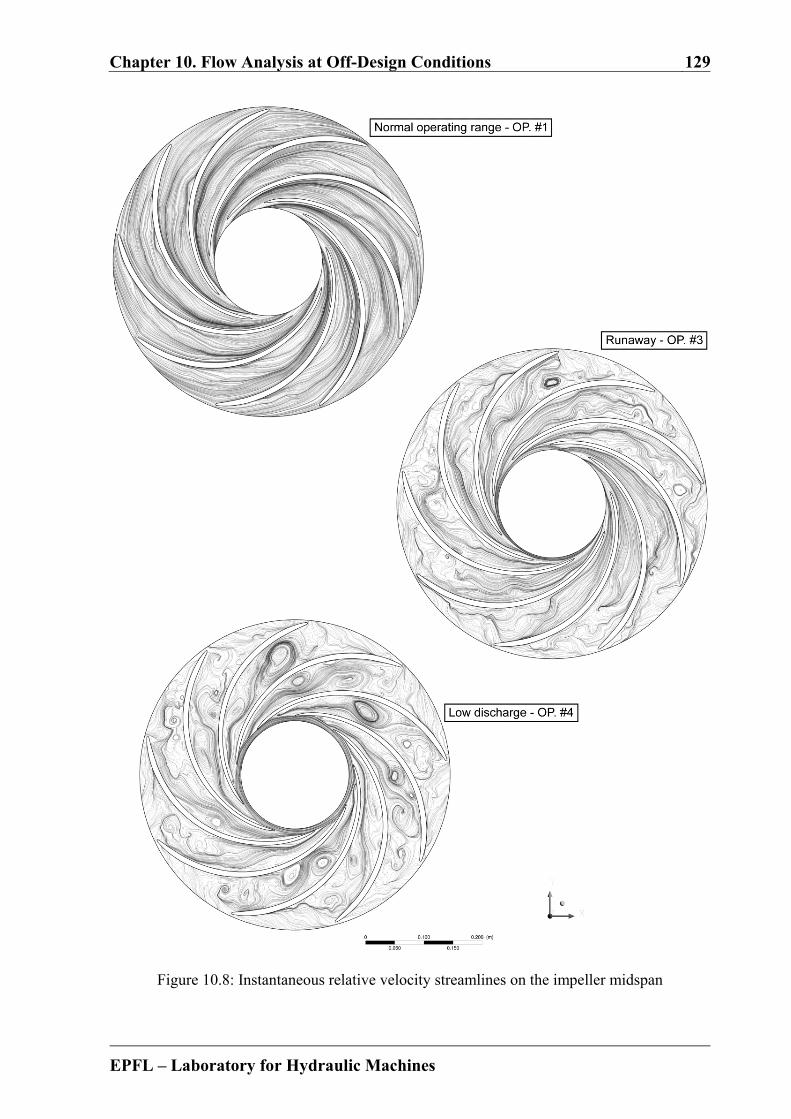
Chapter 10. Flow Analysis at Off-Design Conditions 129
EPFL – Laboratory for Hydraulic Machines
Figure 10.8: Instantaneous relative velocity streamlines on the impeller midspan
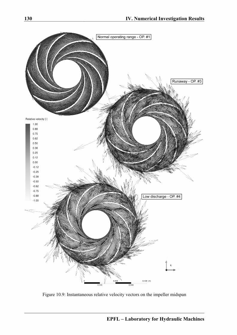
130 IV. Numerical Investigation Results
EPFL – Laboratory for Hydraulic Machines
Figure 10.9: Instantaneous relative velocity vectors on the impeller midspan
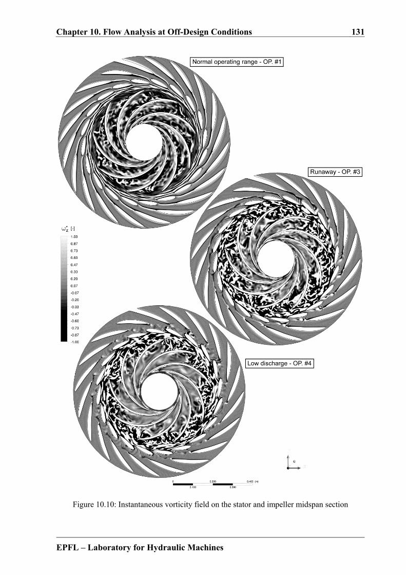
Chapter 10. Flow Analysis at Off-Design Conditions 131
EPFL – Laboratory for Hydraulic Machines
Figure 10.10: Instantaneous vorticity field on the stator and impeller midspan section
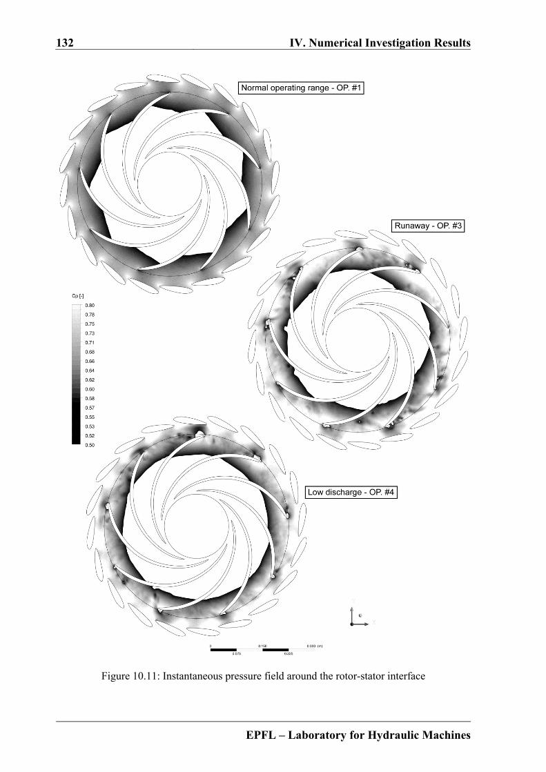
132 IV. Numerical Investigation Results
EPFL – Laboratory for Hydraulic Machines
Figure 10.11: Instantaneous pressure field around the rotor-stator interface

Chapter 10. Flow Analysis at Off-Design Conditions 133
EPFL – Laboratory for Hydraulic Machines
Figure 10.12: Instantaneous pressure field and relative velocity 3D streamlines in the impeller

134 IV. Numerical Investigation Results
EPFL – Laboratory for Hydraulic Machines
Focusing on the impeller, both the instantaneous relative velocity streamlines (Figure 10.8) and the instantaneous relative velocity vectors field on the impeller midspan, normalized with the circumferential velocity at the impeller outlet (Figure 10.9), show that, at the normal operating range, the flow follows the impeller blades profile. In contrast, at off-design conditions, the flow in the impeller is dominated by separation at the inlet and recirculation inside the channels. Moreover, the radial velocity vectors, which are normalized with the discharge velocity at the impeller outlet, reveal irregular backflow on the rotor-stator interface at the runaway and low discharge operating conditions (see Figure 10.6).
Figure 10.13: Instantaneous action lines on walls of two consecutive impeller channels The contour of the instantaneous vorticity ωz
*, defined by equation (5.19), and pressure coefficient (equation (10.4)), around the rotor-stator interface at the midspan section (Figure 10.10 and Figure 10.11, respectively) and the instantaneous relative velocity 3D streamlines in the impeller (Figure 10.12) come to enforce the idea that, at runaway and low discharge conditions, the impeller inlet is dominated by separated flow. Consequently, heterogeneous
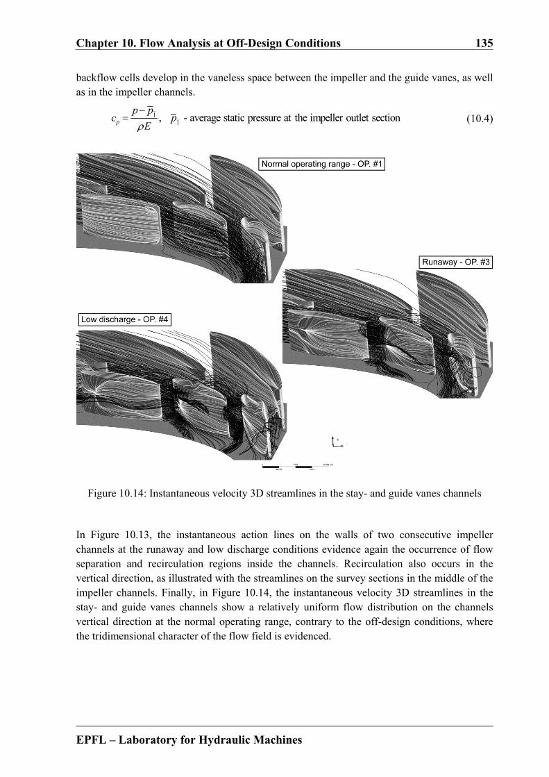
Chapter 10. Flow Analysis at Off-Design Conditions 135
EPFL – Laboratory for Hydraulic Machines
backflow cells develop in the vaneless space between the impeller and the guide vanes, as well as in the impeller channels.
11, - average static pressure at the impeller outlet sectionp
p pc p
E
(10.4)
Figure 10.14: Instantaneous velocity 3D streamlines in the stay- and guide vanes channels In Figure 10.13, the instantaneous action lines on the walls of two consecutive impeller channels at the runaway and low discharge conditions evidence again the occurrence of flow separation and recirculation regions inside the channels. Recirculation also occurs in the vertical direction, as illustrated with the streamlines on the survey sections in the middle of the impeller channels. Finally, in Figure 10.14, the instantaneous velocity 3D streamlines in the stay- and guide vanes channels show a relatively uniform flow distribution on the channels vertical direction at the normal operating range, contrary to the off-design conditions, where the tridimensional character of the flow field is evidenced.

136 IV. Numerical Investigation Results
EPFL – Laboratory for Hydraulic Machines
10.3 Rotating Stall Evidence
According to Brennen [22], the rotating stall is a phenomenon occurring in a cascade of stator- or rotor blades when they operate at high angle of incidence. Moreover, a stall zone appears on few adjacent channels and propagates circumferentially from blade to blade at a fraction of the rotational speed. In the case of a rotor, the stall rotates in the same direction with the impeller, but at 50÷70% of its angular velocity. In our case study, flow separation occurs at runaway and low discharge operating conditions since the relative flow velocity angle at the impeller inlet is strongly reduced, leading to partial blockage of the impeller channels. In Figure 10.15, Figure 10.16 and Figure 10.18, instantaneous velocity streamlines on the stator and impeller midspan section along with the pressure at the rotor-stator interface and the impeller channels discharge are illustrated by using a blade-to-blade view for the normal operating range, runaway and low discharge operating conditions. If, at the normal operating range condition the flow is aligned with the impeller blades and the discharge is relatively uniformly distributed in the impeller channels, at the low discharge condition four impeller channels (respectively the channels with the numbers 4, 6, 8 and 9) are found to be partially blocked, or even to pump (see the impeller channel number 9), whereas the remaining five are overloaded. Nevertheless, at the runaway condition, five consecutive impeller channels (respectively the channels with the numbers 8 to 3) are found to be partially blocked, while the remaining four impeller channels are overloaded. A stalled region over 4 to 5 impeller channels is identified since their discharge is only at about 30% of the nominal value. The low-pass filtered pressure distribution on the rotor-stator interface confirms the location of the stalled region with the decrease of pressure (seen from the right to the left) in front of partially blocked impeller channels (positions Rs59 to Rs67) and the pressure increase in front of overloaded channels (positions Rs67 to Rs78). Indeed, as noticed in the PIV measurements, a phase shift of about π/2 between the guide vanes channel discharge and pressure fluctuations during the rotating stall passage is found again. The stall region rotates in the same direction as the one followed by the impeller, but only with about 55% of the impeller speed. In addition, the instantaneous vorticity contour on the stator and impeller midspan section (Figure 10.17) evidences the presence of separation vortices in the wake of stay vanes when the channels operate in normal turbine way. By contrast, these vortices are missing during the stall passage. As regards the presence of large separation vortices, it is observed at the impeller outlet in front of overloaded channels. To conclude, the main finding of the numerical investigation is that the flow in a low specific speed radial pump-turbine operating at off-design operating conditions in generating mode is dominated by flow separation at the impeller inlet. As noticed in the experiments, when operating at runaway condition, an increase in the pressure fluctuations amplitude is observed mainly in the stator. Moreover, one single stall cell is found to rotate with the impeller at subsynchronous speed in the vaneless gap between the impeller and the guide vanes. It is the effect of flow separation developed at the inlet of several consecutive impeller channels that leads to their blockage.
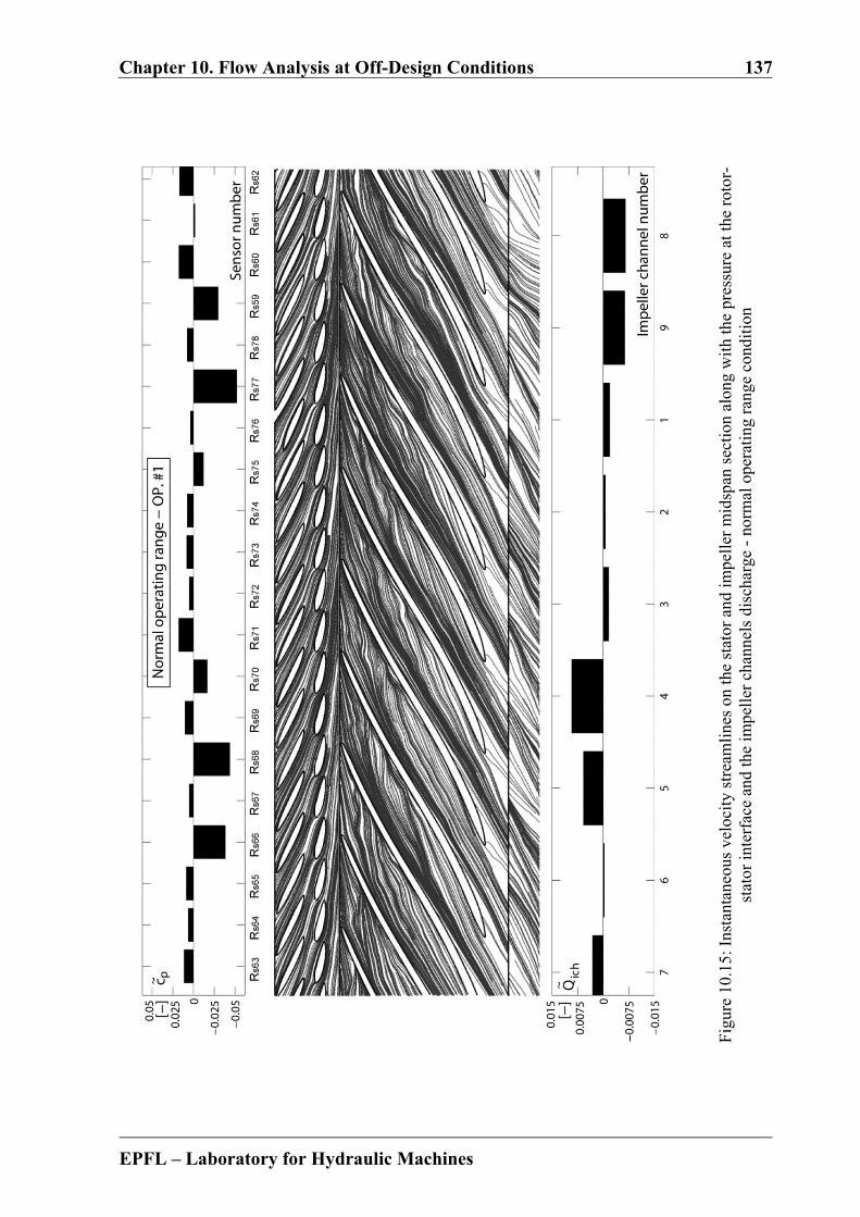
Chapter 10. Flow Analysis at Off-Design Conditions 137
EPFL – Laboratory for Hydraulic Machines
Fig
ure
10.1
5: I
nsta
ntan
eous
vel
ocit
y st
ream
line
s on
the
stat
or a
nd im
pell
er m
idsp
an s
ecti
on a
long
wit
h th
e pr
essu
re a
t the
rot
or-
stat
or in
terf
ace
and
the
impe
ller
cha
nnel
s di
scha
rge
- no
rmal
ope
rati
ng r
ange
con
diti
on
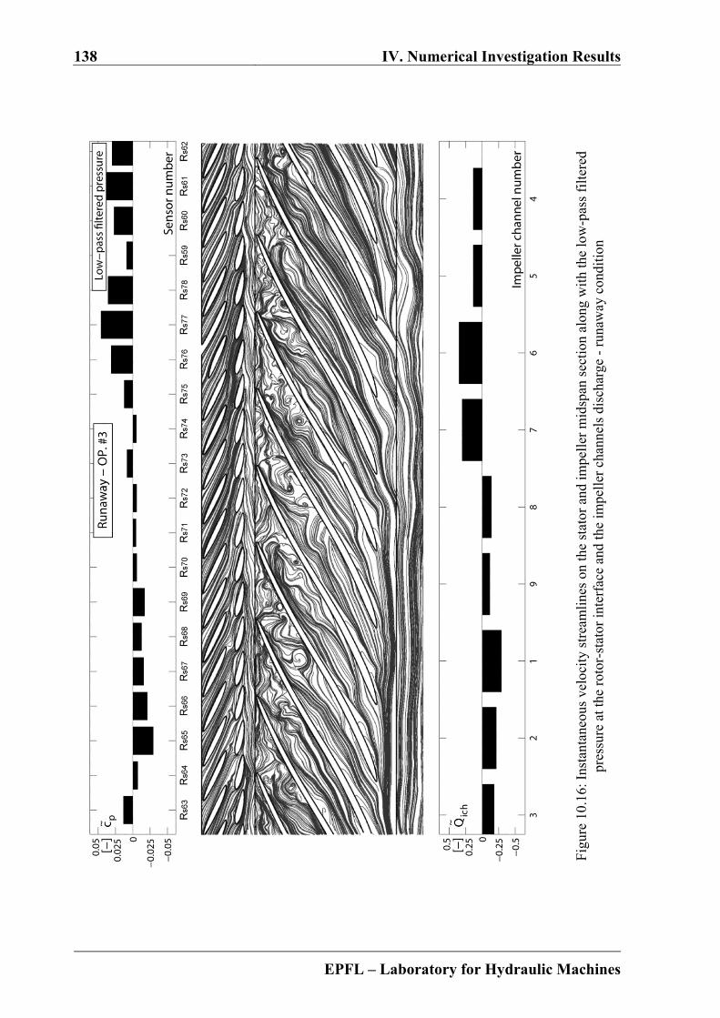
138 IV. Numerical Investigation Results
EPFL – Laboratory for Hydraulic Machines
Fig
ure
10.1
6: I
nsta
ntan
eous
vel
ocit
y st
ream
line
s on
the
stat
or a
nd im
pell
er m
idsp
an s
ecti
on a
long
wit
h th
e lo
w-p
ass
filt
ered
pr
essu
re a
t the
rot
or-s
tato
r in
terf
ace
and
the
impe
ller
chan
nels
dis
char
ge -
run
away
con
diti
on

Chapter 10. Flow Analysis at Off-Design Conditions 139
EPFL – Laboratory for Hydraulic Machines
Fig
ure
10.1
7: I
nsta
ntan
eous
vor
tici
ty ω
z* on
the
stat
or a
nd im
pell
er m
idsp
an s
ecti
on a
long
wit
h th
e lo
w-p
ass
filt
ered
pre
ssur
e at
the
roto
r-st
ator
inte
rfac
e an
d th
e im
pell
er c
hann
els
disc
harg
e -
runa
way
con
diti
on

140 IV. Numerical Investigation Results
EPFL – Laboratory for Hydraulic Machines
Fig
ure
10.1
8: I
nsta
ntan
eous
vel
ocit
y st
ream
line
s on
the
stat
or a
nd im
pell
er m
idsp
an s
ecti
on a
long
wit
h th
e lo
w-p
ass
filt
ered
pr
essu
re a
t the
rot
or-s
tato
r in
terf
ace
and
the
impe
ller
cha
nnel
s di
scha
rge
– lo
w d
isch
arge
con
diti
on
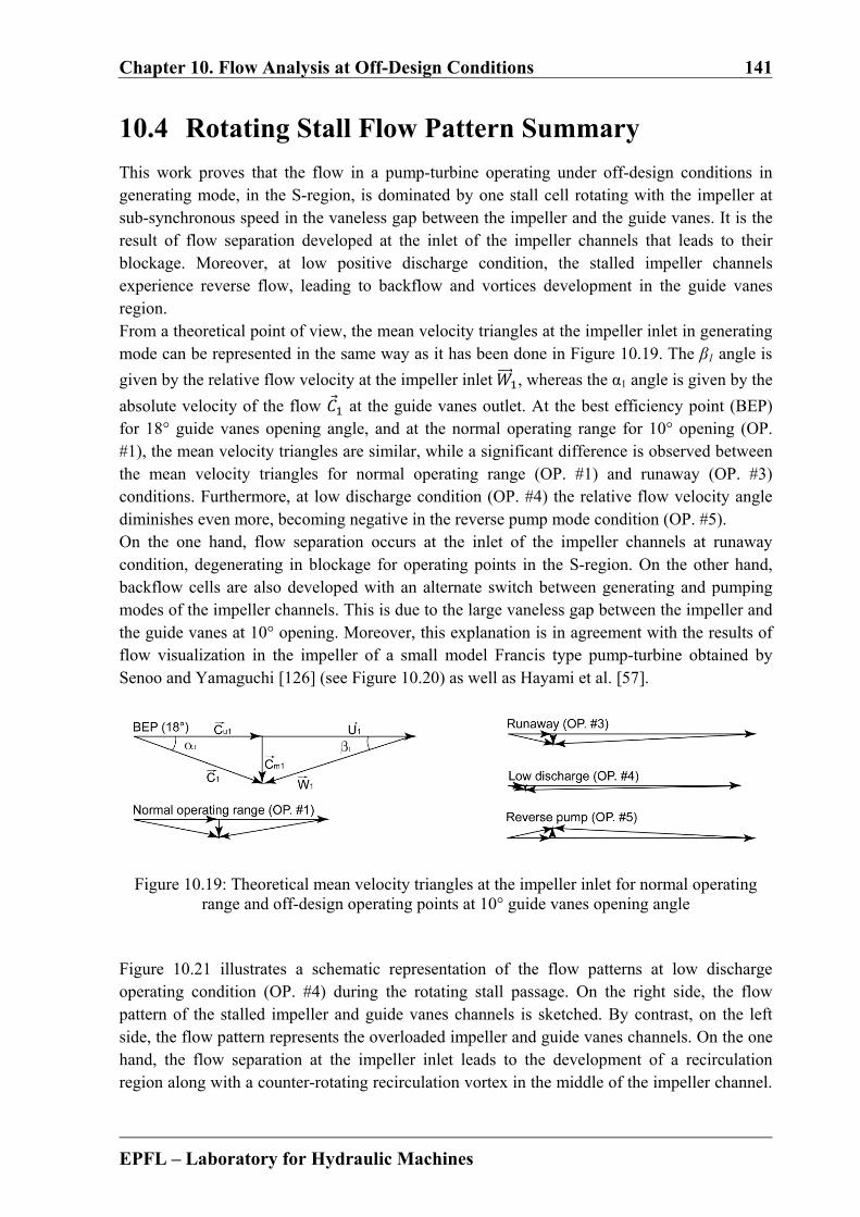
Chapter 10. Flow Analysis at Off-Design Conditions 141
EPFL – Laboratory for Hydraulic Machines
10.4 Rotating Stall Flow Pattern Summary
This work proves that the flow in a pump-turbine operating under off-design conditions in generating mode, in the S-region, is dominated by one stall cell rotating with the impeller at sub-synchronous speed in the vaneless gap between the impeller and the guide vanes. It is the result of flow separation developed at the inlet of the impeller channels that leads to their blockage. Moreover, at low positive discharge condition, the stalled impeller channels experience reverse flow, leading to backflow and vortices development in the guide vanes region. From a theoretical point of view, the mean velocity triangles at the impeller inlet in generating mode can be represented in the same way as it has been done in Figure 10.19. The β1 angle is
given by the relative flow velocity at the impeller inlet , whereas the α1 angle is given by the
absolute velocity of the flow at the guide vanes outlet. At the best efficiency point (BEP) for 18° guide vanes opening angle, and at the normal operating range for 10° opening (OP. #1), the mean velocity triangles are similar, while a significant difference is observed between the mean velocity triangles for normal operating range (OP. #1) and runaway (OP. #3) conditions. Furthermore, at low discharge condition (OP. #4) the relative flow velocity angle diminishes even more, becoming negative in the reverse pump mode condition (OP. #5). On the one hand, flow separation occurs at the inlet of the impeller channels at runaway condition, degenerating in blockage for operating points in the S-region. On the other hand, backflow cells are also developed with an alternate switch between generating and pumping modes of the impeller channels. This is due to the large vaneless gap between the impeller and the guide vanes at 10° opening. Moreover, this explanation is in agreement with the results of flow visualization in the impeller of a small model Francis type pump-turbine obtained by Senoo and Yamaguchi [126] (see Figure 10.20) as well as Hayami et al. [57].
Figure 10.19: Theoretical mean velocity triangles at the impeller inlet for normal operating range and off-design operating points at 10° guide vanes opening angle
Figure 10.21 illustrates a schematic representation of the flow patterns at low discharge operating condition (OP. #4) during the rotating stall passage. On the right side, the flow pattern of the stalled impeller and guide vanes channels is sketched. By contrast, on the left side, the flow pattern represents the overloaded impeller and guide vanes channels. On the one hand, the flow separation at the impeller inlet leads to the development of a recirculation region along with a counter-rotating recirculation vortex in the middle of the impeller channel.
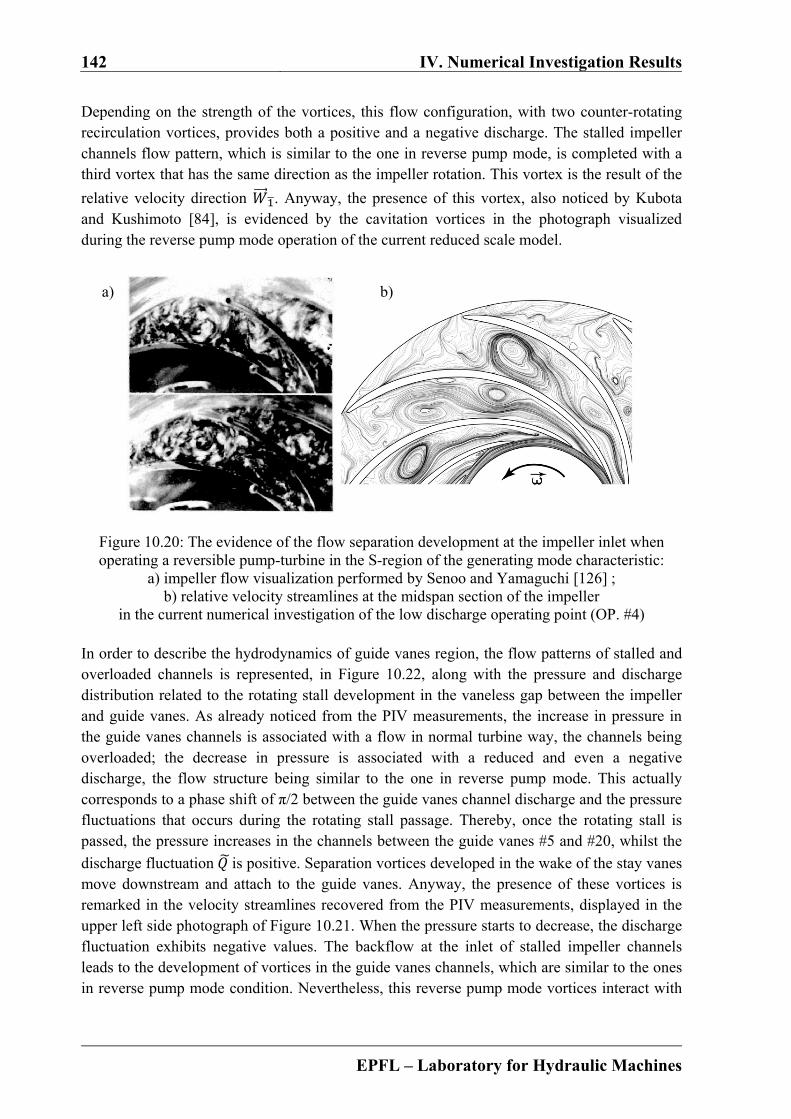
142 IV. Numerical Investigation Results
EPFL – Laboratory for Hydraulic Machines
Depending on the strength of the vortices, this flow configuration, with two counter-rotating recirculation vortices, provides both a positive and a negative discharge. The stalled impeller channels flow pattern, which is similar to the one in reverse pump mode, is completed with a third vortex that has the same direction as the impeller rotation. This vortex is the result of the
relative velocity direction . Anyway, the presence of this vortex, also noticed by Kubota and Kushimoto [84], is evidenced by the cavitation vortices in the photograph visualized during the reverse pump mode operation of the current reduced scale model.
Figure 10.20: The evidence of the flow separation development at the impeller inlet when operating a reversible pump-turbine in the S-region of the generating mode characteristic:
a) impeller flow visualization performed by Senoo and Yamaguchi [126] ; b) relative velocity streamlines at the midspan section of the impeller
in the current numerical investigation of the low discharge operating point (OP. #4) In order to describe the hydrodynamics of guide vanes region, the flow patterns of stalled and overloaded channels is represented, in Figure 10.22, along with the pressure and discharge distribution related to the rotating stall development in the vaneless gap between the impeller and guide vanes. As already noticed from the PIV measurements, the increase in pressure in the guide vanes channels is associated with a flow in normal turbine way, the channels being overloaded; the decrease in pressure is associated with a reduced and even a negative discharge, the flow structure being similar to the one in reverse pump mode. This actually corresponds to a phase shift of π/2 between the guide vanes channel discharge and the pressure fluctuations that occurs during the rotating stall passage. Thereby, once the rotating stall is passed, the pressure increases in the channels between the guide vanes #5 and #20, whilst the
discharge fluctuation is positive. Separation vortices developed in the wake of the stay vanes move downstream and attach to the guide vanes. Anyway, the presence of these vortices is remarked in the velocity streamlines recovered from the PIV measurements, displayed in the upper left side photograph of Figure 10.21. When the pressure starts to decrease, the discharge fluctuation exhibits negative values. The backflow at the inlet of stalled impeller channels leads to the development of vortices in the guide vanes channels, which are similar to the ones in reverse pump mode condition. Nevertheless, this reverse pump mode vortices interact with
a) b)

Chapter 10. Flow Analysis at Off-Design Conditions 143
EPFL – Laboratory for Hydraulic Machines
Fig
ure
10.2
1: S
chem
atic
rep
rese
ntat
ion
of f
low
pat
tern
s at
low
dis
char
ge o
pera
ting
con
diti
on (
OP
. #4)
dur
ing
the
rota
ting
sta
ll p
assa
ge
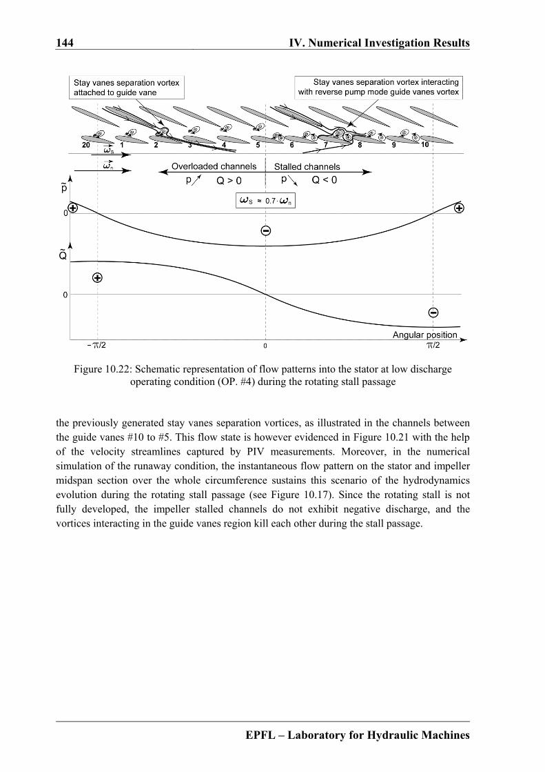
144 IV. Numerical Investigation Results
EPFL – Laboratory for Hydraulic Machines
Figure 10.22: Schematic representation of flow patterns into the stator at low discharge operating condition (OP. #4) during the rotating stall passage
the previously generated stay vanes separation vortices, as illustrated in the channels between the guide vanes #10 to #5. This flow state is however evidenced in Figure 10.21 with the help of the velocity streamlines captured by PIV measurements. Moreover, in the numerical simulation of the runaway condition, the instantaneous flow pattern on the stator and impeller midspan section over the whole circumference sustains this scenario of the hydrodynamics evolution during the rotating stall passage (see Figure 10.17). Since the rotating stall is not fully developed, the impeller stalled channels do not exhibit negative discharge, and the vortices interacting in the guide vanes region kill each other during the stall passage.

EPFL – Laboratory for Hydraulic Machines
Part V
Conclusions

EPFL – Laboratory for Hydraulic Machines
Chapter 11
Conclusions and Perspectives
11.1 Conclusions
The present work contributes to the understanding of the hydrodynamics of a low specific speed Francis type pump-turbine operating at off-design conditions in generating mode, experiencing unstable operation at runaway. The reason of this instability is due to the presence of a positive slope on the discharge-speed as well as torque-speed characteristics. The findings of this study show that the operation in the so-called “S-shaped” region of the characteristic is governed by flow separation developed at the inlet of the impeller channels. Moreover, at runaway speed, the flow separation leads to the onset of one stall cell rotating with the impeller at sub-synchronous frequency (about 70% of the impeller rotational frequency), which further increases in intensity when moving on the positive slope of the characteristic toward zero discharge and reverse pump conditions. The case study is a low specific speed radial pump-turbine reduced scale model whose characteristic curves at openings equal or greater than 7.5° exhibit a positive slope after the runaway speed. This work focuses particularly on normal operating range, runway and very low positive discharge operating conditions at 10° guide vanes opening angle. The methods employed in this process are the experimental and the numerical simulation ones. The experiments performed in this research involve: high-speed flow visualizations using either tuft or injected air bubbles, PIV measurements in the stator, and wall pressure measurements in both stationary and rotating frames. When starting from the normal operation and augmenting the impeller speed a significant increase in pressure fluctuations, mainly in the guide vanes region, is noticed. Spectral analysis of pressure measurements in the stator shows a rise of a low frequency component (70% of the impeller rotational frequency) at runaway, which further increases as zero discharge is approached. Analysis of the instantaneous pressure peripheral distribution in the vaneless gap reveals one stall cell rotating with the impeller at sub-synchronous speed. The same low frequency component, with slightly lower amplitude compared to the rotor-stator interface location, is identified in the rotating frame pressure measurements as well. One may notice that in the rotating frame referential, the stall cell covering about half of the impeller circumference (4 to 5 channels) revolves at subsynchronous frequency (about 30% of the impeller rotational frequency) in counterclockwise direction.

148 V. Conclusions
EPFL – Laboratory for Hydraulic Machines
When using injected air bubbles and tuft, high-speed flow visualizations reveal a quite uniform flow pattern in the guide vanes channels at the normal operating range. In contrast, when being at runaway, the flow is highly disturbed by the rotating stall passage. The situation is even more critical at very low positive discharge, where backflow and vortices develop in the guide vanes channels during the stall passage. Afterwards, a specific image processing technique applied on the high-speed movies reconstructs the rotating stall evolution in the entire guide vanes circumference for the low positive discharge condition. The presence of backflow and vortices in the guide vanes channels during the stall passage is also evidenced with the high-speed tuft visualizations. In addition, during the stall passage, the wires position in the guide vanes as well as at the impeller outlet suggests a flow state that is similar to the one in reverse pump mode operation. PIV measurements in the guide vanes region confirm the outflow at the impeller inlet. The flow state in the guide vanes region turned out to be similar to the one in reverse pump mode. Moreover, it is found that the pumping phenomenon in the guide vanes channels is performed with the help of a vortex. This corresponds to the way in which the flow may change the direction by 180°, going from the vaneless gap to the upstream side of guide vanes. Therefore, at the low positive discharge condition, the flow alternates between turbine and reverse pump modes during one rotating stall revolution. The unsteady incompressible turbulent flow numerical simulation is performed in the full reduced scale model water passage domain by employing the Ansys CFX code for the selected operating points. The incompressible unsteady Reynolds-Averaged Navier-Stokes equations are solved by applying the finite volume method. The hybrid RANS-LES turbulence model based on the von Karman length scale for blending function, called SAS-SST, is employed in simulation. Wall pressure measurements in both stationary and rotating frames are used to validate the numerical results. It is important to clarify that the current study uses the advantages of the numerical simulation in order to investigate the development of flow instabilities mainly in the rotating frame, where, even in a reduced scale model, the experimental measurements are too expensive or technically limited. The pressure fluctuations, produced by the rotor-stator interaction, are in good agreement with the experiments for both normal operating range and off-design conditions. By contrast, the rotating stall is captured at runaway. As for the expected organized rotating stall, it is not well defined at low discharge operating condition, even if several impeller channels are found to pump. Despite the fact that numerical simulation results are not quantitatively accurate, their qualitative analysis is used to draw the flow pattern inside the impeller in the presence of rotating stall. Thereby, it is shown that two stationary counter-rotating large vortices dominate the impeller channels flow. Their source is the large flow separation at the impeller inlet. This flow configuration can provide both a positive and a negative discharge, with a smooth transition between the turbine and reverse pump modes. In addition, a third vortex is generated at the impeller outlet during the reverse pump mode because of the relative velocity direction. To sum up, the flow in a pump-turbine operating under off-design conditions in generating mode, in the S-region, is dominated by one stall cell rotating with the impeller at sub-synchronous speed in the vaneless gap between the impeller and the guide vanes. It is the result of flow separation developed at the inlet of the impeller channels that leads to their
Chapter 11. Conclusions and Perspectives 149
EPFL – Laboratory for Hydraulic Machines
blockage. Moreover, at low positive discharge condition, the stalled impeller channels are found to pump, leading to backflow and vortices development in the guide vanes region. The rotating instability generates hydraulic unbalance and strong structural vibrations.
11.2 Perspectives
Modern pump-turbines are subject to frequent switching between pumping and generating modes with extended operation under off-design conditions. Depending on the specific speed of the pump-turbine, the discharge-speed as well as the torque-speed generating mode characteristics at constant guide vanes opening can be “S-Shaped”. In such a situation, the machine operation can become strongly unstable at runaway speed and beyond, with a significant increase in structural vibrations and noise. Moreover, since a stable runaway operating point is difficult to be reached, the synchronization with the electrical network in safety conditions becomes impossible. This study emphasizes the fact that the flow in a pump-turbine operating under off-design conditions in generating mode, in the S-region, is dominated by one stall cell rotating with the impeller at sub-synchronous speed in the vaneless gap between the impeller and the guide vanes. It is the result of flow separation developed at the inlet of the impeller channels that leads to their blockage. Furthermore, it is worth reminding the reader that, at low positive discharge condition, the stalled impeller channels are found to pump, thus leading to backflow and vortices development in the guide vanes region. Therefore, the rotating stall onset is found to be connected with the presence of the positive slope on the characteristic curve. Further investigations on reversible pump-turbines with different design should confirm this relationship. The active control of flow separation at the impeller inlet represents a possible solution that could be adopted in order to avoid the onset of rotating stall and the positive slope on the characteristic curves. It is known that the impeller of a reversible pump-turbine is mainly designed for pump mode operation. From a practical point of view, this means that a single-stage reversible pump-turbine is by nature forced to be operated as a compromise between an optimum pump and an optimum turbine (Billdal and Wedmark [13]). Attention should be paid to the overall performance in order to obtain the advantages of a simplified and cost-effective pump-storage design concept. Nevertheless, few technical solutions already exist that allow operators to stabilize the machine during the start-up or in case of a sudden load rejection. One of them is the so-called Misaligned Guide Vanes (MGV) concept (Klemm [80], Bouschon et al. [17] and Shao [128]), which consists in operating, through the use of independent servomotors, several guide vanes independently from the rest of the guide vane mechanism in order to stabilize the machine. The principle adopted by this technique consists in shifting a stable characteristic curve, 6° guide vanes opening for the current case, to the required characteristic curve, 10° guide vanes opening, by correcting the discharge with the help of several guide vanes largely opened. However, more research is needed to better understand the hydrodynamics behind this method.
150 V. Conclusions
EPFL – Laboratory for Hydraulic Machines
To conclude, the numerical simulation of rotating separated flows, either in turbine or pump mode, still represents a great challenge for the available turbulence models and/or computational resources. Whereas URANS models are not suitable for separated flows with attached boundary layer, a turbulence model like LES, already employed in turbomachinery applications with promising results by Kato et al. [78], or even DNS, could provide better results. However it would require too much computational resources for the so large computational domain that is the entire pump-turbine. Although in terms of computational power and time, for a fine enough mesh, the hybrid SAS-SST turbulence model proves to be the most suitable one for the present case, the results show the need of a more appropriate hybrid model for this type of application. Such a turbulence model could be, for example, a DNS with wall modeling.

EPFL – Laboratory for Hydraulic Machines
Bibliography


EPFL – Laboratory for Hydraulic Machines
References
[1] Adkins, F.E., 1987, “Raccoon Mountain Pumped-Storage Plant - Ten Years Operating
Experience”, IEEE - Transactions on Energy Conversion, EC-2(3), pp. 361-368
[2] Al-Qutub, A., Khalifa, A., and Khulief, Y., 2009, “Experimental Investigation of The Effect of Radial Gap and Impeller Blade Exit on Flow-Induced Vibration at the Blade-Passing Frequency in a Centrifugal Pump”, International Journal of Rotating Machinery, 2009, Article ID 704845
[3] Amblard, H., Henry, P., Borciani, G., Martin, G., Guiton, P., and Thalmann, R., 1985, “Behavior of Francis Turbines and Pump-Turbines at Partial Flow”, La Houille Blanche, 40(5), pp. 435-440
[4] Ansys Inc., 2009, “ANSYS CFX-Solver Theory Guide”, Release 12.0
[5] Atencio, G., 1981, “Reversible Pump-Turbine”, US Patent No. 4275989
[6] Ausoni, Ph., 2009, “Turbulent Vortex Shedding from a Blunt Trailing Edge Hydrofoil”, PhD Thesis No. 4475, EPFL, Lausanne, Switzerland
[7] Avellan, F., 2010, “Course of Hydraulic Turbomachines - 2010”, École Polytechnique Fédérale de Lausanne, Switzerland
[8] Barbier, E., 2002, “Geothermal Energy Technology and Current Status: An Overview”, Renewable and Sustainable Energy Reviews, 6(1-2), pp. 3-65
[9] Batchelor, G.K., 1981, “An Introduction to Fluid Dynamics”, Cambridge University Press, Great Britain
[10] Batten, P., Goldberg, U., Peroomian, O., and Chakravarthy, S., 2009, “Recommendations and Best Practice for the Current State of the Art in Turbulence Modeling”, International Journal of Computational Fluid Dynamics, 23(4),pp. 363-374
[11] Berten, S., 2010, “Hydrodynamics of High Specific Power Pumps for Off-Design Operating Conditions”, PhD Thesis No. 4642, EPFL, Lausanne, Switzerland
[12] Beyer, T., 2007, “Goldisthal Pumped-Storage Plant: More than Power Production”, Hydro Review Worldwide, 15(1)
[13] Billdal, J.T., and Wedmark, A., 2007, “Recent Experiences with Single Stage Reversible Pump Turbines In GE Energy’s Hydro Business”, Hydro 2007, Granada, Spain, Paper No. 10.3

154 References
EPFL – Laboratory for Hydraulic Machines
[14] Blanchon, F., Planchard, J., and Simonnot, D.V., 1972, “Regimes Transitoires des Groupes Reversibles - Aspects Techniques et Economiques”, La Houille Blanche, 27(6-7), pp. 547-562
[15] Blazek, J., 2001, “Computational Fluid Dynamics: Principles and Applications”, Elsevier Science, Oxford, UK
[16] Borciani, G., and Thalmann, R., 1982, “Influence of Cavitation on Average and Instantaneous Characteristics of Turbines and Pump-Turbines”, La Houille Blanche, 37(2), pp. 197-207
[17] Bouschon, M., Roulet, D., Miscioscia, T., and Pepin, P., 2008, “Recent Achievements in Hydro Actuators”, Hydro 2008, Ljubljana, Slovenia, Paper No. 13.4
[18] Bovet, T., 1963, “Contribution à l'Etude du Tracé d'Aubage d'une Turbine à Réaction du Type Francis”, Informations Techniques Charmilles, 9, pp. 47-70
[19] Bovet, T., and Henry, P., 1970, “Le Nouveau Stand d'Essai Universel pour Machines Hydrauliques à Réaction”, EPFL-IMH, Publication No. 6, Lausanne, Switzerland
[20] Braun, O., 2009, “Part Load Flow in Radial Centrifugal Pumps”, PhD Thesis No. 4422, EPFL, Lausanne, Switzerland
[21] Braza, M., El Akoury, R., Martinat, G., Hoarau, Y., Harran, G., and Chassaing, P., 2006, “Turbulence Modeling Improvement For Highly Detached Unsteady Aerodynamic Flows by Statistical and Hybrid Approaches”, European Conference on Computational Fluid Dynamics, Netherlands
[22] Brennen, C.E., 1994, “Hydrodynamics of Pumps”, Concepts ETI and Oxford University Press, USA
[23] Byskov, K.R., Jacobsen, B.C., and Pedersen, N., 2003, “Flow in a Centrifugal Pump Impeller at Design and Off-Design Conditions—Part II: Large Eddy Simulations”, Journal of Fluids Engineering, Transactions of the ASME, 125(1), pp. 73-83
[24] Calendray, J.F., Ilhat, D., Planchard, J., Lauro, J.F., and Velo, C., 1986, “Analysis of Transient Phenomena in Hydroelectric Generation Plants”, La Houille Blanche, 41(1/2), pp. 149-157
[25] Casacci, S., Boussuges, P., Amblard, H., and Guiton, P., 1972, “Aspects Techniques Propres aux Turbines-Pompes: Influence sur les Caracteristiques Generales de l'Installation et sur la Conception des Machines. Exemples de Realisation”, La Houille Blanche, 27(6-7), pp. 515-528
[26] Chen, Y.N., Haupt, U., and Rautenberg, M., 1990, “Rossby Waves and Associated Transient Rotating Stall Vortices in Radial and Axial Turbocompressors”, Zeitschrift fur Flugwissenschaften und Weltraumforschung, 14, pp. 223-246
[27] Ciocan, G.D., and Kueny, J.-L., 2006, “Experimental Analysis of Rotor-Stator Interaction in a Pump-Turbine”, Proceedings of the 23rd IAHR Symposium on Hydraulic Machinery and Systems, Yokohama, Japan
[28] Columbia Encyclopedia, 2011, In Encyclopædia Britannica, Retrieved from http://www.britannica.com/EBchecked/topic/126960/Columbia-Encyclopedia
References 155
EPFL – Laboratory for Hydraulic Machines
[29] Corson, D., Jaiman, R., and Shakib, F., 2009, “Industrial Application of RANS Modeling: Capabilities and Needs”, International Journal of Computational Fluid Dynamics, 23(4), pp. 337-347
[30] Courier, M., 1982, “Share of Energy Transfer by Pumping in EDF's Park of Generating Facilities and Development of Grand'Maison”, La Houille Blanche, 37(5/6), pp. 403-420
[31] Dantec Dynamics, 2010, “Particle Image Velocimetry Measurement Principles”, Retrieved from www.dantecdynamics.com
[32] Davidson, L., 2003, “An Introduction to Turbulence Models”, Publication 97/2, Chalmers University of Technology, Goteborg, Sweden
[33] Dazin, A., Cavazzini, G., Pavesi, G., Dupont, P., Coudert, S., Ardizzon, G., Caignaert, G., and Bois, G., 2011, “High-Speed Stereoscopic PIV Study of Rotating Instabilities in a Radial Vaneless Diffuser”, Experiments in Fluids, 51(1), pp. 83-93
[34] De Boer, W.W., Verheij, F.J., Zwemmer, D., and Das, R., 2007, “The Energy Island - An Inverse Pump Accumulation Station”, EWEC 2007, Milan, Italy
[35] Deane, J.P.,O Gallachoir, B.P., and McKeogh, E.J., 2010, “Techno-Economic Review of Existing and New Pumped Hydro Energy Storage Plant”, Renewable and Sustainable Energy Reviews, 14(4), pp. 1293-1302
[36] Dengel, P., and Fernholz, H.H., 1990, “An Experimental Investigation of an Incompressible Turbulent Boundary Layer in the Vicinity of Separation”, Journal of Fluid Mechanics, 212, pp. 615-636
[37] Derakhshan, S., and Nourbakhsh, A., 2008, “Experimental Study of Characteristic Curves of Centrifugal Pumps Working as Turbines in Different Specific Speeds”, Experimental Thermal and Fluid Science, 32(3), pp. 800-807
[38] Dixon, S.L., 1961, “Some Three-Dimensional Effects of Rotating Stall”, Aeronautical Research Council Current Papers, 609
[39] Dörfler, P.K., 2010, “Improved Suter Transform for Pump-Turbine Characteristics”, International Journal of Fluid Machinery and Systems, 3(4), pp. 332-341
[40] Dörfler, P.K., Engineer, A.J., Pendse, R.N., Huvet, P., and Brahme, M.V., 1998, “Stable Operation Achieved on a Single-Stage Reversible Pump-Turbine Showing Instability at No-Load”, Proceedings of the 19th IAHR Symposium on Hydraulic Machinery and Cavitation, Singapore, pp. 431-440
[41] Egorov, Y., Menter, F.R., Lechner, R., and Cokljat, D., 2010, “The Scale-Adaptive Simulation Method for Unsteady Turbulent Flow Predictions. Part 2: Application to Complex Flows”, Flow, Turbulence and Combustion, 85(1), pp. 139–165
[42] Egorov, Y., and Menter, F.R., 2008, “Development and Application of SST-SAS Turbulence Model in the DESIDER Project”, In Peng S.-H. Haase W. editors, Advances in Hybrid RANS-LES Modeling - Notes on Numerical Fluid Mechanics and Multidisciplinary Design, Springer-Verlag, Berlin, pp. 261-270
[43] Emmons, H.W., Kronauer, R.E., and Rockett, J.A., 1959, “A Survey of Stall Propagation - Experiment and Theory”, Journal of Basic Engineering, 81, pp. 409-416

156 References
EPFL – Laboratory for Hydraulic Machines
[44] Farhat, M., Natal, S., Avellan, F., Paquet, F., Lowys, Py., and Couston, M., 2002, “Onboard Measurements of Pressure and Strain Fluctuations in a Model of Low Head Francis Turbine - Part 1: Instrumentation”, Proceedings of The of the 21st IAHR Symposium on Hydraulic Machinery and Systems, Lausanne, Switzerland
[45] Farhat, M., Avellan, F., and Seidel, U., 2002, “Pressure Fluctuation Measurements in Hydro Turbine Models”, Proceedings of The 9th International Symposium on Transport Phenomena and Dynamics of Rotating Machinery, Honolulu, Hawaii
[46] Fay, A.A., 2009, “Does Rotating Stall Occur in Francis Runners Causing Fluctuations?”, Proceedings of the 3rd International Meeting of the Workgroup on Cavitation and Dynamic Problems in Hydraulic Machinery and Systems, Brno, Czech Republic, pp. 45-54
[47] Ferziger, J.H., and Peric, M., 1999, “Computational Methods for Fluid Dynamics”, 2nd Revised Edition, Springer-Verlag, Berlin, Germany
[48] Frigne, P., and Van Den Braembussche, R., 1984, “Distinction Between Different Types of Impeller and Diffuser Rotating Stall in a Centrifugal Compressor with Vaneless Diffuser”, Journal of Engineering for Gas Turbines and Power, Transactions of the ASME, 106, pp. 468-474
[49] Fujihara, T., Imano, H., and Oshima, K., 1998, “Development of Pump Turbine for Seawater Pumped-Storage Power Plant”, Hitachi Review, 47(5)
[50] Garg, H.P., Mullick, S.C., and Bhargava, A.K., 1985, “Solar Thermal Energy Storage”, Reidel Publishing Company, Holland
[51] Gokhman, A., 1985, “Reversible Two-Stage Hydraulic Machine”, US Patent No. 4496282
[52] Guyon, E., Hulin, J.P., and Petit, L., 2001, “Hydrodynamique Physique”, EDP Sciences, France
[53] Hasmatuchi, V., Farhat, M., Roth, S., Botero, F., and Avellan, F., 2011, “Experimental Evidence of Rotating Stall in a Pump-Turbine at Off-Design Conditions in Generating Mode”, Journal of Fluids Engineering, Transactions of the ASME, 133(5)
[54] Hasmatuchi, V., Roth, S., Botero, F., Farhat, M., and Avellan, F., 2011, “Hydrodynamics of a Pump-Turbine at Off-Design Operating Conditions: Numerical Simulation”, Proceedings of ASME-JSME-KSME Joint Fluids Engineering Conference 2011, Hamamatsu, Japan
[55] Hasmatuchi, V., Roth, S., Botero, F., Avellan, F., and Farhat, M., 2010, “High-Speed Flow Visualization in a Pump-Turbine under Off-Design Operating Conditions”, IOP Conference Series: Earth and Environmental Science, 12(1), doi:10.1088/1755-1315/12/1/012059
[56] Hasmatuchi, V., Farhat, M., Maruzewski, P., and Avellan, F., 2009, “Experimental Investigation of a Pump-Turbine at Off-Design Operating Conditions”, Proceedings of the 3rd International Meeting of the Workgroup on Cavitation and Dynamic Problems in Hydraulic Machinery and Systems, Brno, Czech Republic, pp. 339-347
[57] Hayami, H., Chen, D., and Koso, T., 1995, “Application of Image Processing Measurement to a Relative Flow in a Pump-Turbine Runner”, Journal of Flow Visualization and Image Processing, 2, pp. 75-82

References 157
EPFL – Laboratory for Hydraulic Machines
[58] Henry, P., 1992, “Turbomachines Hydrauliques - Choix Illustre de Realisations Marquantes”, Presses Polytechniques et Universitaires Romandes, Switzerland
[59] Hewlett-Packard, 1999, “HP E1432A 16 Channel 51.2 kSa/s Digitizer plus DSP - User’s Guide”, Part Number E1432-90013, Hewlett-Packard Company, Washington, USA
[60] Hirsch, C., and Tartinville, B., 2009, “Reynolds-Averaged Navier-Stokes Modeling for Industrial Applications and Some Challenging Issues”, International Journal of Computational Fluid Dynamics, 23(4), pp. 295-303
[61] Hoarau, Y., Braza, M., Ventikos, Y., Faghani, D., and Tzabiras, G., 2003, “Organized Modes and the Three-Dimensional Transition to Turbulence in the Incompressible Flow Around a NACA0012 Wing”, Journal of Fluid Mechanics, 496, pp. 63-72
[62] Horsley, A., and Wrobel, A.J., 2002, “Efficiency Rents of Pumped-Storage Plants and Their Uses for Operation and Investment Decisions”, Journal of Economic Dynamics and Control, 27(4), pp. 109-142
[63] Host-Madsen, A., and McCluskey, D.R., 1994, “On the Accuracy and Reliability of PIV Measurements”, Proceedings of the 7th International Symposium on Applications of Laser Techniques of Flow Measurements, Lisbon, Portugal
[64] Houdeline, J.-B., Bouvet, Y., Bazin, D., Couston, M., Francois, M., and Verzeroli, J.-M., 2006, “Double Stage Regulated and Reversible Pump Turbines of Yangyang Power Station in Korea”, Proceedings of the 23rd IAHR Symposium on Hydraulic Machinery and Systems, Yokohama, Japan, Paper No. F260
[65] Hu, H., and Yang, Z., 2008, “An Experimental Study of the Laminar Flow Separation on a Low-Reynolds-Number Airfoil”, Journal of Fluids Engineering, Transactions of the ASME, 130(5)
[66] Huber Instrumente, 1994, “Etalons de Transfert de Pression Types PRF/PHF 3000 - Mode d'Emploi”, Liestal, Switzerland
[67] Hutarew, G., 1975, “Pumped Storage Power Plant”, US Patent No. 3891860
[68] Huvet, P., 1992, “Steady Oscillatory Conditions Between Pump-Turbine Operating at Partial Flow and Surge Shaft”, Proceedings of the 16th IAHR Symposium on Hydraulic Machinery and Cavitation, Sao Paulo, Brazil, pp. 349-358
[69] Ikeda, K., Inagaki, M., Niikura, K., and Oshima, K., 2000, “700-m 400-MW Class Ultrahigh-Head Pump Turbine”, Hitachi Review, 49(2), pp. 81-87
[70] Ingram, E.A., 2010, “Worldwide Pumped Storage Activity”, Hydro Review Worldwide, 18(4)
[71] International Electrotechnical Committee, 1999, “Hydraulic Turbines, Storage Pumps and Pump-Turbines – Model Acceptance Tests”, International Standard IEC 60193, 2nd Edition
[72] International Energy Agency, 2010, “Key World Energy Statistics”, Paris, France
[73] International Energy Agency, 2010, “Renewables Information 2010”, Paris, France
[74] Jelusic, F., 1974, “Multi-Stage Pump-Turbine”, US Patent No. 3794456
158 References
EPFL – Laboratory for Hydraulic Machines
[75] Johnson, D.A., Pedersen, N., and Jacobsen, C.B., 2005, “Measurements of Rotating Stall Inside a Centrifugal Pump Impeller”, Proceedings of FEDSM2005 - ASME Fluids Engineering Division Summer Meeting and Exhibition, Houston, TX, USA, pp. 1281-1288
[76] Joselin Herbert, G.M., Iniyan, S., Sreevalsan, E., and Rajapandian, S., 2005, “A Review of Wind Energy Technologies”, Renewable and Sustainable Energy Reviews, 11, pp. 1117-1145
[77] Kaltenbach, H.-J., Fatica, M., Mittal, R., Lund, T.S., and Moin, P., 1999, “Study of Flow in a Planar Asymmetric Diffuser Using Large-Eddy Simulation”, Journal of Fluid Mechanics, 390, pp. 151-185
[78] Kato C., Mukai H., and Manabe A., 2003, “Large-Eddy Simulation of Unsteady Flow in a Mixed-Flow Pump”, International Journal of Rotating Machinery, 9, pp. 345–351
[79] Keane D.R., and Adrian, J.R., 1992, “Theory of Cross-Correlation Analysis of PIV Images”, Applied Scientific Research, 49(3), pp. 191-215
[80] Klemm, D., 1982, “Stabilizing the Characteristics of a Pump-Turbine in The Range Between Turbine Part-Load and Reverse Pumping Operation”, Voith Forschung und Konstruktion, 28, Paper 2
[81] Kline, J.S., 1959, “On the Nature of Stall”, Journal of Basic Engineering, 81,pp. 305-320
[82] Koutnik, J., Foust, J., Nicolet, C., Saiju, R., and Kawkabani, B., 2010, “Pump-Storage Integration with Renewables - Meeting the Needs Using Various Concepts”, Proceedings of HydroVision International, Charlotte, NC, USA
[83] Krause, N., Zahringer, K., and Pap, E., 2005, “Time-Resolved Particle Imaging Velocimetry for the Investigation of Rotating Stall in a Radial Pump”, Experiments in Fluids, 39(2), pp. 192-201
[84] Kubota, T., and Kushimoto, S., 1980, “Visual Observation of Internal Flow Through High-Head Pump-Turbine”, Fuji Electric Review, 26(4), pp. 133-144
[85] Kuwabara, T., Katayama, K., Nakagawa, H., and Hagiwara, H., 2000, “Improvements of Transient Performance of Pump Turbine upon Load Rejection”, Power Engineering Society Summer Meeting, Seattle, WA, USA, 3, pp. 1783-1788
[86] Lacoste, A., 1980, “Life of Pump-Turbine Components Undergoing Numerous Changes in Operating Conditions During Daily Service”, La Houille Blanche, 35(1/2), pp. 141-146
[87] Landry, C., Alligné, S., Hasmatuchi, V., Roth, S., Mueller, A., and Avellan, F., 2011, “Non-Linear Stability Analysis of a Reduced Scale Model Pump-Turbine at Off-Design Operation”, Proceedings of the 4th International Meeting on Cavitation and Dynamic Problems in Hydraulic Machinery and Systems, Belgrade, Serbia
[88] Launder, B.E., 1989, “Second-Moment Closure and Its Use in Modelling Turbulent Industrial Flows”, International Journal for Numerical Methods in Fluids, 9(8),pp. 963-985
[89] Lavigne, S., Duarte, F., Houdeline, J.-B., and Verzeroli, J.-M., 2010, “Experience with Low Head Reversible Pump-Turbine Design: The Alqueva Pumped-Storage Plant in Portugal”, Hydro 2010, Lisbon, Portugal, Paper No. 2.1
References 159
EPFL – Laboratory for Hydraulic Machines
[90] Leishman, J.G., 1990, “Dynamic Stall Experiments on the NACA 23012 Aerofoil”, Experiments in Fluids, 9(1-2), pp. 49-58
[91] Lesieur, M., 1997, “Turbulence in Fluids”, Kluwer Academic, Dordrecht / Boston / London
[92] Lewis, N.S., 2007, “Toward Cost-Effective Solar Energy Use”, Science, 315(5813), pp. 798-801
[93] Ley, R.D., 1968, “Hydroelectric Pump-Turbine Apparatus”, US Patent No. 3405278
[94] Liang, Q., Keller, M., and Sick, M., 2009, “Rotor-Stator Interaction During No Load Operation of Pump-Turbines”, Hydro 2009, Lyon, France, Paper No. 7.08
[95] Liees, C., Fischer, G., Hilgendorf, J., and Lux, M., 1986, “Causes and Remedy of Fatigue Cracks in Runners”, International Symposium on Fluid Machinery Troubleshooting, Anaheim, California, USA, 46(2), pp. 43-52
[96] Ljevar, S., de Lange, H.C., and van Steenhoven, A.A., 2006, “Two-Dimensional Rotating Stall Analysis in a Wide Vaneless Diffuser”, International Journal of Rotating Machinery, 12, pp. 1-11
[97] Mankbadi, R.R., and Mikhail, A.S., 1985, “A Turbine-Pump System for Low-Head Hydropower”, Energy Conversion and Management, 25(3), pp. 339-344
[98] Martin, C.S., 1997, “Effect of Pump-Turbine Characteristics Near Runaway on Instability”, Proceedings of the Centennial International Conference on Fluid Engineering, Tokyo, Japan
[99] Martin, C.S., 2000, “Instability of Pump-Turbines with S-Shaped Characteristics”, Proceedings of the 20th IAHR Symposium on Hydraulic Machinery and Systems, Charlotte, USA
[100] McCroskey, W.J., 1982, “Unsteady Airfoils”, Annual Review of Fluid Mechanics, 14, pp. 285-311
[101] McKendry, P., 2002, “Energy Production from Biomass (Part 2): Conversion Technologies”, Bioresource Technology, 83(1), pp. 47-54
[102] Menter, F.R., 2009, “Review of the Shear-Stress Transport Turbulence Model Experience from an Industrial Perspective”, International Journal of Computational Fluid Dynamics, 23(4), pp. 305-316
[103] Menter, F.R., Kuntz, M., and Langtry, R., 2003, “Ten Years of Industrial Experience with the SST Turbulence Model”, Turbulence, Heat and Mass Transfer, 4, Begell House Inc., pp. 625–632
[104] Menter, F.R., and Egorov, Y., 2005, “SAS Turbulence Modeling of Technical Flows”, Proceedings of the 6th International ERCOFTAC Workshop on Direct and Large-Eddy Simulation, Poitiers, France
[105] Menter, F.R., and Egorov, Y., 2010, “The Scale-Adaptive Simulation Method for Unsteady Turbulent Flow Predictions. Part 1: Theory and Model Description”, Flow, Turbulence and Combustion, 85(1), pp. 113-138
[106] Miyabe, M., Maeda, H., Umeki, I., and Jittani, Y., 2006, “Unstable Head-Flow Characteristic Generation Mechanism of a Low Specific Speed Mixed Flow Pump”, Journal of Thermal Science, 15(2), pp. 115-121
160 References
EPFL – Laboratory for Hydraulic Machines
[107] Nant de Drance Project Web Site, www.nant-de-drance.ch
[108] National Instruments, 2008, “24-Bit, 102.4 kS/s, 8- and 4-Channel Dynamic Signal Acquisition - NI 4472 Series, NI PCI-4474”, Retrieved from www.ni.com
[109] Nicolet, C., Alligne, S., Kawkabani, B., Koutnik, J., Simond, J-J., and Avellan, F., 2009, “Stability Study of Francis Pump-Turbine at Runaway”, Proceedings of the 3rd International Meeting of the Workgroup on Cavitation and Dynamic Problems in Hydraulic Machinery and Systems, Brno, Czech Republic, pp. 371-384
[110] Nicolet, C., 2007, “Hydroacoustic Modeling and Numerical Simulation of Unsteady Operation of Hydroelectric Systems”, PhD Thesis No. 3751, EPFL, Lausanne, Switzerland
[111] Nowicki, P., Sallaberger, M., and Bachmann, P., 2009, “Modern Design of Pump-Turbines”, IEEE Electrical Power & Energy Conference, Montreal, Canada, pp. 1-7
[112] Oishi, A., and Yokoyama, T., 1980, “Development of High-Head Single- and Double-Stage Reversible Pump-Turbines”, Proceedings of the 10th IAHR Symposium on Hydraulic Machinery and Cavitation, Tokyo, Japan, pp. 441-452
[113] Parrondo-Gayo, L.J., Gonzalez-Perez, J., and Fernandez-Francos, J., 2002, “The Effect of the Operating Point on the Pressure Fluctuations at the Blade Passage Frequency in the Volute of a Centrifugal Pump”, Journal of Fluids Engineering, Transactions of the ASME, 124(3), pp. 784-790
[114] Pedersen, N., Larsen, S.P., and Jacobsen, B.C., 2003, “Flow in a Centrifugal Pump Impeller at Design and Off-Design Conditions - Part I: Particle Image Velocimetry (PIV) and Laser Doppler Velocimetry (LDV) Measurements”, Journal of Fluids Engineering, Transactions of the ASME, 125(1), pp. 61-72
[115] Pejovic, S., Krsmanovic, L., Jemcov, R., and Crnkovic, P., 1976, “Unstable Operation of High-Head Reversible Pump-Turbines”, Proceedings of the 8th IAHR Symposium on Hydraulic Machinery and Cavitation, Leningrad, Russia, pp. 283-295
[116] Pelc, R., and Fujita, R.M., 2002, “Renewable Energy from The Ocean”, Marine Policy, 26(6), pp. 471-479
[117] Photron, 2007, “Fastcam SA1.1 – Hardware Manual”, Revision 1.00E, Photron Limited, Tokyo, Japan
[118] Rahman, S., 2003, “Green Power: What Is It and Where Can We Find It?”, Power and Energy Magazine, IEEE, 1(1), pp. 30-37
[119] Roberts, B., 2009, “Capturing Grid Power”, Power and Energy Magazine, IEEE, 7(4), pp. 32-41
[120] Roth, S., Hasmatuchi, V., Botero, F., Farhat, M., and Avellan, F., 2011, “Influence of the Pump-Turbine Guide Vanes Vibrations on the Pressure Fluctuations in the Rotor-Stator Vaneless Gap”, Proceedings of The 4th International Meeting on Cavitation and Dynamic Problems in Hydraulic Machinery and Systems, Belgrade, Serbia
[121] Rudnicky, V., 1972, “The Importance of Pumped-Storage Stations in the Supply Economics of Power Systems”, Power Technology and Engineering, Formerly Hydrotechnical Construction, 6(6), pp. 551-557
References 161
EPFL – Laboratory for Hydraulic Machines
[122] Rumsey, C.L., and Swanson, R.C., 2009, “Turbulence Modeling for Active Flow Control Applications”, International Journal of Computational Fluid Dynamics, 23(4), pp. 317-326
[123] Ryhming, I.L., 2004, “Dynamique des Fluides - 2eme Edition”, Presses Polytechniques et Universitaires Romandes, Lausanne, Switzerland
[124] Sagaut, P., 2005, “Large Eddy Simulation for Incompressible Flows: An Introduction”, 3rd Edition, Springer, Berlin, Germany
[125] Sano, T., Yoshida, Y., Tsujimoto, Y., Nakamura, Y., and Matsushima, T., 2002, “Numerical Study of Rotating Stall in a Pump Vaned Diffuser”, Journal of Fluids Engineering, Transactions of the ASME, 124(2), pp. 363-370
[126] Senoo, Y., and Yamaguchi, M., 1987, “A Study on Unstable S-Shape Characteristic Curves of Pump Turbines at No-Flow”, Journal of Turbomachinery, 109, pp. 77-82
[127] Shannon, C.E., 1949, “Communication in the Presence of Noise”, Proceedings of the IRE, 37(1), pp. 10-21
[128] Shao, W.Y., 2009, “Improving Stability by Misaligned Guide Vanes in Pumped Storage Plant”, Asia-Pacific Power and Energy Engineering Conference, Wuhan, China, pp. 1-5
[129] Sharp, R.E.B., 1941, “Hydraulic Power-Accumulation System”, US Patent No. 2246472
[130] Simpson, L.R., 1989, “Turbulent Boundary-Layer Separation”, Annual Review of Fluid Mechanics, 21, pp. 205-234
[131] Sinha, M., Pinarbasi, A., and Katz, J., 2001, “The Flow Structure During Onset and Developed States of Rotating Stall Within a Vaned Diffuser of a Centrifugal Pump”, Journal of Fluids Engineering, Transactions of the ASME, 123(3), pp. 490-499
[132] Sioshansi, R., Denholm, P., Jenkin, T., and Weiss, J., 2009, “Estimating the Value of Electricity Storage in PJM: Arbitrage and Some Welfare Effects”, Energy Economics, 31(2), pp. 269-277
[133] Smith, F.T., 1986, “Steady and Unsteady Boundary-Layer Separation”, Annual Review of Fluid Mechanics, 18, pp. 113-144
[134] Spalart, P.R., 2001, “Young-Person's Guide to Detached-Eddy Simulation Grids”, NASA / CR-2001-211032
[135] Spalart, P.R., 2009, “RANS Modeling into a Second Century”, International Journal of Computational Fluid Dynamics, 23(4), pp. 291-293
[136] Staubli, T., Senn, F., and Sallaberger, M., 2008, “Instability of Pump-Turbines During Start-Up in the Turbine Mode”, Hydro 2008, Ljubljana, Slovenia, Paper No. 9.6
[137] Stelzer, R.S., and Walters, R.N., 1977, “Estimating Reversible Pump-Turbine Characteristics”, US Department of The Interior Bureau of Reclamation
[138] Stenning, A.H., 1980, “Rotating Stall and Surge”, Journal of Fluids Engineering, Transactions of the ASME, 102(1), pp. 14-20

162 References
EPFL – Laboratory for Hydraulic Machines
[139] Stepanik, H.E., and Brekke, H., 1990, “Unsteady Flow Phenomena in a Reversible Francis Pump Turbine”, Fluid Machinery Forum, 96, pp. 9-14, Presented at the 1990 Spring Meeting of the Fluids Engineering Division
[140] Swiss Federal Office of Energy, 2010, “Graphiques de la Statistique Suisse de l’Electricité 2009”, Switzerland
[141] Tanaka, H., and Tsunoda, S., 1980, “The Development of High Head Single Stage Pump-Turbines”, Proceedings of the 10th IAHR Symposium on Hydraulic Machinery and Cavitation, Tokyo, Japan, pp. 429-440
[142] Tanaka, H., 1990, “Vibration Behavior and Dynamic Stress of Runners of Very High Head Reversible Pump-Turbines”, Proceedings of the 15th IAHR Symposium on Hydraulic Machinery and Cavitation, Belgrade, Yugoslavia
[143] Taulan, J.P., 1986, “Overpressure Peak in Dual Horizontal Francis Turbines - Industrial Experiments Results”, La Houille Blanche, 41(1/2), pp. 127-135
[144] Tennessee Valley Authority, 1981, “Hiwassee Dam Unit 2 Reversible Pump-Turbine (1956) - A National Historic Mechanical Engineering Landmark”, Retrieved from www.asme.org
[145] Tietjen, J.S., 2007, “Pumped Storage Hydroelectricity”, Encyclopedia of Energy Engineering and Technology, 3, pp. 1207-1212
[146] Vesely, J., Pulpitel, L., and Troubil, P., 2006, “Model Research of Rotating Stall on Pump-Turbines”, Hydro 2006, Porto Carras, Greece, Paper No. 3.5
[147] von Nessen-Lapp, W., and Nowicki, P., 2004, “Goldisthal - 4x265 MW Pumpturbines in Germany: Special Mechanical Design Features and Comparison Between Stationary and Variable Speed Operation”, Proceedings of the 22nd IAHR Symposium on Hydraulic Machinery and Systems, Stockholm, Sweden, Paper No. A15-4
[148] Vorus, W.S., 1983, “A Theory for Flow Separation”, Journal of Fluid Mechanics, 132, pp. 163-183
[149] Wang, L.Q., Yin, J.L., Jiao, L., Wu, D.Z., and Qin, D.Q., 2011, “Numerical Investigation on the “S” Characteristics of a Reduced Pump Turbine Model”, Science China - Technological Sciences, doi: 10.1007/s11431-011-4295-2
[150] White, F.M., 2009, “Fluid Mechanics”, McGraw-Hill International, USA
[151] Widmer, C., Staubli, T., Tresch, T., and Sallaberger, M., 2010, “Unstable Pump-Turbine Characteristics and Their Interaction with Hydraulic Systems”, HydroVision, Charlotte, North-Carolina, USA
[152] Widmer, C., Staubli, T., and Ledergerber, N., 2011, “Unstable Characteristics and Rotating Stall in Turbine Brake Operation of Pump-Turbines”, Journal of Fluids Engineering, Transactions of the ASME, 133(4)
[153] Williams, C.J., 1977, “Incompressible Boundary-Layer Separation”, Annual Review of Fluid Mechanics, 9, pp. 113-144
[154] Wirschal, H.H., 1971, “Reversible Pump/Turbines for Raccoon Mountain”, International Pumped Storage Conference, Wisconsin Univ.
References 163
EPFL – Laboratory for Hydraulic Machines
[155] Wuibaut, G., Bois, G., Dupont, P., Caignaert, G., and Stanislas, M., 2002, “PIV Measurements in the Impeller and the Vaneless Diffuser of a Radial Flow Pump in Design and Off-Design Operating Conditions”, Journal of Fluids Engineering, Transactions of the ASME, 124(3), pp. 791-797
[156] Younsi, M., Djerrada, A., Belamri, T., and Menter, F., 2008, “Application of the SAS Turbulence Model to Predict the Unsteady Flow Field Behavior in a Forward Centrifugal Fan”, International Journal of Computational Fluid Dynamics, 22(9),pp. 639–648
[157] Zingg, D.W., and Godin, P., 2009, “A Perspective on Turbulence Models for Aerodynamic Flows”, International Journal of Computational Fluid Dynamics, 23(4), pp. 327-335
[158] Zobeiri, A., 2009, “Investigations of Time Dependent Flow Phenomena in a Turbine and a Pump-Turbine of Francis Type: Rotor-Stator Interactions and Precessing Vortex Rope”, PhD Thesis No. 4272, EPFL, Lausanne, Switzerland
[159] Zobeiri, A., Kueny, J.-L., Farhat, M., and Avellan, F., 2006, “Pump-Turbine Rotor-Stator Interactions in Generating Mode: Pressure Fluctuation in Distributor Channel”, Proceedings of the 23rd IAHR Symposium on Hydraulic Machinery and Systems, Yokohama, Japan

Biography 165
EPFL – Laboratory for Hydraulic Machines
Curriculum Vitae
Vlad HASMATUCHI
Rue des Grands Vergers 11 CH-1964 Conthey (VS) Switzerland
Tel: +41 78 921 06 19 E-mail: [email protected]
December 04, 1983Arad, Romania Married
EDUCATION
2008-2011 PhD in Engineering Science École Polytechnique Fédérale de Lausanne (EPFL), Switzerland
2002-2007 Mechanical Engineer Diploma University “Politehnica” of Timisoara, Romania Faculty of Mechanical Engineering, Hydraulic Machinery Branch Diploma Project accomplished between March-June 2007 at EPFL, Laboratory for Hydraulic Machines, Switzerland
1998-2002 High School “Grup Scolar Industrial Transporturi Cai Ferate Arad“, Romania Specialization in Informatics
PROFESSIONAL EXPERIENCE
2012- University of Applied Sciences of Western Switzerland Institute of Systems Engineering, Sion, Valais
Senior Research Assistant
2007-2011 École Polytechnique Fédérale de Lausanne (EPFL), Switzerland Laboratory for Machines Hydrauliques
Doctoral Assistant
PhD Thesis: Hydrodynamics of a Pump-Turbine Operating at Off-Design Conditions in Generating Mode
Research Projects
Hydrodyna II - Eureka 4150 - Industrial partners: Andritz Hydro, Voith Hydro, Alstom Hydro - Academic partners: EPFL-LMH, UPC-CDIF - Financial support: Swisselectric Research, KTI/CTI
Hydronet I - Industrial partners: KWO - Academic partners: EPFL, EMPA, EAWAG, HSLU - Financial support: CCEM, Swisselectric Research
Teaching Activities
Course of Specialization in Hydraulic Machines Coordination of Master Projects Preparation of exercises and exams sessions

166 Biography
EPFL – Laboratory for Hydraulic Machines
2005-2007 University “Politehnica” of Timisoara (UPT), Romania National Center for Engineering of Systems with Complex Fluids Numerical Simulation and Parallel Computing Laboratory
Research Assistant (50%) Main Research Activity: Numerical Analysis of the Effect of Water Jet Injection on the Flow Behavior in a Francis Turbine Draft Tube at Part Load Operating Point
2005 I.C.P.V. Arad – Trinity Rail Group SA, Romania
Training (1 month) on railway and tank wagons design and manufacturing
DIPLOMAS AND AWARDS
Diplomas Course of Specialization in Hydraulic Machines – 2008, EPFL – LMH Switzerland
Certificate of Pedagogical Competence – 2007, UPT Romania
Course of Numerical Methods in Fluid Dynamics and FLUENT Applications – 2006 National Center for Engineering of Systems with Complex Fluids, UPT Romania
Certificate of Professional Competence in Informatics – 2002 High School “Grup Scolar Industrial Transporturi Cai Ferate Arad“, Romania
Awards Graduation with “Highest Honors” of Batchelor and Master Studies
Graduation with “Highest Honors” of High School
Honor Prize “Eminent Student of the Mechanical Engineering Faculty” Agency “Orizonturi Universitare” of Timisoara, Romania - 2006
Honorable Mention at the Machines Mechanisms competition, “Organolog” UPT local phase, Romania, 2005 edition
Honorable Mention at the Materials Resistance competition, “C.C. Teodorescu” national phase, Romania, 2004 edition
Second Prize at the AutoCAD 2D Drawings competition, “StudentCAD” UPT local phase, Romania, 2004 edition
Third Prize at the AutoCAD 3D Drawings competition, “StudentCAD” UPT local phase, Romania, 2004 edition
First Prize at the Mechanics competition, “Traian Lalescu” UPT local phase, Romania, 2004 edition
Third Prize at the AutoCAD 2D Drawings competition, “StudentCAD” UPT local phase, Romania, 2003 edition
INFORMATICS
OS MS-DOS, Windows, Linux
Programming Pascal, C, Fortran, Perl, FoxPro, Matlab, Mathcad, Xmgr
CFD Gambit, Fluent, Techplot, Ansys ICEM, Ansys CFX, Paraview
CAD AutoCAD, SolidWorks, Inventor
Office MS-Office, LaTeX
Multimedia MS-Office, Windows Movie Maker, Adobe Illustrator & Photoshop, Matlab
LANGUAGES
Romanian Native speaker
English Fluent (C2)
French Fluent (C2)
German Beginner (A1)

Biography 167
EPFL – Laboratory for Hydraulic Machines
List of Publications
Journal Articles
1. Hasmatuchi, V., Farhat, M., Roth, S., Botero, F., and Avellan, F., 2011, “Experimental Evidence of Rotating Stall in a Pump-Turbine at Off-Design Conditions in Generating Mode”, Journal of Fluids Engineering, Transactions of the ASME, 133(5)
2. Susan-Resiga, R., Muntean, S., Hasmatuchi, V., Anton, I., and Avellan F., 2010, “Analysis and Prevention of Vortex Breakdown in the Simplified Discharge Cone of a Francis Turbine”, Journal of Fluids Engineering, Transactions of the ASME, 132(5)
3. Maruzewski, P., Hasmatuchi, V., Mombelli, H. P., Burggraeve, D., Iosfin, J., Finnegan, P., and Avellan, F., 2009, “Surface Roughness Impact on Francis Turbine Performances and Prediction of Efficiency Step Up”, International Journal of Fluid Machinery and Systems, 2(3), pp. 353-362
Conference Papers
1. Roth, S., Hasmatuchi, V., Botero, F., Farhat, M., and Avellan, F., 2011, “Influence of the Pump-Turbine Guide Vanes Vibrations on the Pressure Fluctuations in the Rotor-Stator Vaneless Gap”, Proceedings of the 4th International Meeting on Cavitation and Dynamic Problems in Hydraulic Machinery and Systems, Belgrade, Serbia
2. Landry, C., Alligné, S., Hasmatuchi, V., Roth, S., Muller, A., and Avellan, F., 2011, “Non-Linear Stability Analysis of a Reduced Scale Model Pump-Turbine at Off-Design Operation”, Proceedings of the 4th International Meeting on Cavitation and Dynamic Problems in Hydraulic Machinery and Systems, Belgrade, Serbia
3. Hasmatuchi, V., Roth, S., Botero, F., Farhat, M., and Avellan, F., 2011, “Hydrodynamics of a Pump-Turbine at Off-Design Operating Conditions: Numerical Simulation”, Proceedings of the 7th International Symposium on Pumping Machinery, Hamamatsu, Japan
4. Hasmatuchi, V., Mohamed, F., Roth, S., Botero, F., and Avellan, F., 2011, “Hydrodynamics of a Pump-Turbine Operating at Off-Design Conditions: Experimental Investigation”, SHF Conference on Cavitation and Hydraulic Machines, Lausanne, Switzerland
5. Hasmatuchi, V., Roth, S., Botero, F., Avellan, F., and Farhat, M., 2010, “High-Speed Flow Visualization in a Pump-Turbine under Off-Design Operating Conditions”, IOP Conference Series: Earth and Environmental Science, 12(1), doi: 10.1088/1755-1315/12/1/012059
6. Roth, S., Hasmatuchi, V., Botero, F., Farhat, M., and Avellan, F., 2010, “Fluid-Structure Coupling in the Guide Vanes Cascade of a Pump-Turbine Scale Model”, IOP Conference Series: Earth and Environmental Science, 12(1), doi: 10.1088/1755-1315/12/1/012074
168 Biography
EPFL – Laboratory for Hydraulic Machines
7. Roth, S., Hasmatuchi, V., Botero, F., Farhat, M., and Avellan, F., 2010, “Advanced Instrumentation for Measuring Fluid-Structure Coupling Phenomena in the Guide Vanes Cascade of a Pump-Turbine Scale Model”, Proceedings of the 7th International Symposium on Fluid-Structure Interactions, Flow-Sound Interactions, and Flow-Induced Vibration & Noise, Montreal, Canada
8. Hasmatuchi, V., Farhat, M., and Avellan, F., 2010, “Hydrodynamics of a Pump-Turbine under Off-Design Operating Conditions in Generating Mode”, Proceedings of the 1st EPFL Doctoral Conference in Mechanics, Lausanne, Switzerland, pp. 111-114
9. Alligne, S., Nicolet, C., Ruchonnet, N., Hasmatuchi, V., Maruzewski, P., and Avellan, F., 2009, “Numerical Simulation of Nonlinear Self Oscillations of a Full Load Vortex Rope”, Proceedings of the 3rd IAHR International Meeting of the Workgroup on Cavitation and Dynamic Problems in Hydraulic Machinery and Systems, 2, Brno, Czech Republic, pp. 325-338
10. Hasmatuchi, V., Farhat, M., Maruzewski, P., and Avellan, F., 2009, “Experimental Investigation of a Pump-Turbine at Off-Design Operating Conditions”, Proceedings of the 3rd IAHR International Meeting of the Workgroup on Cavitation and Dynamic Problems in Hydraulic Machinery and Systems, 2, Brno, Czech Republic, pp. 339-347
11. Maruzewski, P., Hasmatuchi, V., Mombelli, H. P., Burggraeve, D., Iosfin, J., Finnegan, P., and Avellan, F., 2008, “Surface Roughness Impact on Francis Turbine Performances and Prediction of Efficiency Step Up”, Proceedings of the 24th IAHR Symposium on Hydraulic Machinery and Systems, Foz do Iguassu, Brazil
12. Susan-Resiga, R., Muntean, S., Hasmatuchi, V., and Bernad, S., 2007, “Development of a Swirling Flow Control Technique for Francis Turbines Operated at Partial Discharge” ,Proceedings of the 3rd German-Romanian Workshop on Turbomachinery Hydrodynamics, Timisoara, Romania, pp. 28-40
13. Hasmatuchi, V., and Susan-Resiga, R, 2006, “Numerical Analysis of Swirling Flow Downstream a Hydraulic Turbine Runner”, Zilele Tehnice Studentesti - Volum de Lucrari Stiintifice, pp. 91-95
14. Susan-Resiga, R., Muntean, S., Hasmatuchi, V., Bernad, S., Anton, I., and Avellan F., 2006, “Inviscid Vortex Breakdown in Decelerated Swirling Flows and Flow Control Methods”, 2nd Workshop on Vortex Dominated Flows, Bucharest, Romania