hydrodynamic dispersion during infiltration of water into soil1

Hydrodynamic Dispersion During Infiltration of Water into Soil1

D. E. ELRICK, K. B. LARYEA, AND P. H. GROENEVELT2

ABSTRACTThe analysis of hydrodynamic dispersion during one-dimen-

sional sorption of water by soil (horizontal flow) is extended toinclude 'the gravitational effects present during one-dimensionalinfiltration (vertical flow). A power series form for the solutionis developed in a manner similar to that developed by 'Philipfor water movement during infiltration. Similar to the sorptionanalysis, the longitudinal dispersion coefficient was assumedto be a function of water content only. A computer simulationprogram using CSMP was used to solve the associated differen-tial equations. A single program was found to be suitable aslong as the Boltzman parameter (distance divided by the squareroot of time) was used as the independent variable throughout.An algorithm was developed to give successively better solu-tions of the soil water diffusion and hydrodynamic dispersionequations.

Infiltration experiments were carried out on a clay loam soil.Both the water and chloride content profiles preserved similarityin terms of the Boltzman parameter. Water and solute coeffi-cients of the power series solutions were calculated from hori-zontal infiltration and hydraulic conductivity data and used topredict both the water and solute profiles during vertical in-filtration. Good agreement between the vertical infiltrationdata and the theoretical predictions was obtained.

Additional Index Words: unsaturated soils, transient flow,miscible displacement, computer simulation program (CSMP).

Elrick, D. E., K. B. Laryea, and P. H. Groenevelt. 1979. Hy-drodynamic dispersion during infiltration of water into soil.Soil Sci. Soc. Am. J. 43:856-865.

HYDRODYNAMIC DISPERSION during one-dimensionalsorption of water by soil (horizontal flow) has

been examined recently by Smiles et al. (1978). Thepresent study extends the analysis to include hydrody-namic dispersion during one-dimensional infiltration(vertical flow). In this case, gravitational effects areincluded in the analysis.

Smiles et al. (1978) have shown that Dt, the appar-ent longitudinal dispersion coefficient, may be takenas a function of 0 only, where 6 is the volumetric watercontent. By assuming that any dependence of D3 onv, the volume flux density of the solution, is negligible,the equation describing one-dimensional sorption waspresented as

^-i^wfi-^. mwhere c is the solute concentration in the water, x isthe horizontal space coordinate, and t is time. Notethat we have used 6D, (6) where Smiles et al. (1978)have used D, (0). Scotter and Raats (1970) and Smileset al. (1978) have shown experimentally that both thewater and salt concentration profiles preserve similari-ty during sorption in terms of distance divided by thesquare root of time. Accordingly, the substitution\ = xt~l/z was shown to remove both x and t fromEq. [1] giving

i_ [ M ,w£1 +M<l= 0 ,where

2 dx

g(0) = e\s - I " \wde'6n

Contribution from Department of Land Resource Science,University of Guelph, Guelph, Ontario, Canada. The authorsacknowledge support from the National Research Council ofCanada and the Ontario Ministry of Agriculture and Food.Received 19 Dec. 1977. Approved 23 May 1979.

'Professor, Graduate Student and Professional Associate, re-spectively.

ELRICK ET AL.: HYDRODYNAMIC DISPERSION DURING INFILTRATION OF WATER INTO SOIL 857

and On is the initial value of 0. Note that there is noneed to identify A. when it is the independent variable.However, X will be identified as X«, or \, (whereXw is a function of 0 and X5 is a function of c) whereverX is expressed as the dependent variable or wheneverthere is doubt as to the interpretation.

The corresponding equation for water flow is given

where D(0) is the soil-water diffusivity.

One-Dimensional InfiltrationDuring one-dimensional infiltration the liquid flow

velocity is given byv = K(e) - D(9) dO/dz, [Z]

where z is the vertical space coordinate, taken positivedownward. During infiltration the water content dis-tribution may be described by

37 [3]

where K(6) is the hydraulic conductivity.Use of the equation of continuity and substitution

of Eq. [2] into Eq. [1] gives the following equationfor the salt concentration distribution:

wExperimentally, a constant source of solution of a

different salt concentration is applied to one end ofa column of soil having an initially uniform volu-metric water content and solution salt concentration.

With respect to the water, the following conditionsapply:

0 = 6n, z > 0, t = 0 [5a]0 = eot z = 0, t ^ 0. [5b]

With respect to the solute, the initial condition isc = cn, z > 0, t = 0. [6a]

As discussed by Smiles et al. (1978), two forms of theboundary condition for the solute are possibly appro-priate; viz the constant concentration boundary con-dition:

c = c0, z = 0, tor the flux boundary condition

0, [6b]

-6Ds(e) = v(c0 - c), z = 0, t ^ 0. [6c]

Equations [3] and [4] may be rewritten with zas the dependent variable:

_ 9 z = d_ D(9) ,3t 36 L3z/30J L J

• ]•3c L3z/3cPhilip (1957) developed the following power series

form for the solution of Eq. [7] subject to conditions[5a] and [5b].z = xw(6)t [9]

The functions X^e), xw(0), <l/w(6), <*w(0), etc. are eachgoverned by separate ordinary differential equationsfor which Philip (1955, 1957) developed numericalmethods of solution. Using a technique similar to thatdeveloped by Philip (1957), a power series in t1'2may also be used to obtain a solution of Eq. [8] ; viz.

z = xs(c)t [10]

Details of the above solution are provided in the Ap-pendix. The results are summarized in Table 1.

Equation [11], [13], [15], and [17] in Table 1are highly nonlinear in 9 and numerical methods ofsolution have been developed by Philip (1955, 1957).On the other hand, solute Eq. [12] is linear in c andmay be solved in explicit form. The calculation ofc(\) when Ds(0) is known depends first on the valuesof 0(\) and then on the observation that since 0(A) isunique, Eq. [12] may be written as the linear equa-tion

[25]

[26]

[27a][27b]

[28]

where

g(X) = 0\s H»-AA

The solution of Eq. [12]) subject toc = cn, X —» oo,c — c0, X = 0,

yields (Smiles et al., 1978):c — CQCn — C0

with

M(X) =

[->/2 pJo[29]

The solution to the flux balance boundary condi-tion,

= - (c - c0)D(6)

= o

and

is given byc - c0 _ 2 + S M(X)Cn - C0 ~ 2 + S M(oo)

The sorptivity S is given by

[27c]

[30]

858 SOIL SCI. SOC. AM. J., VOL. 43, 1979

Table 1—Ordinary differential equations for water and solute transport.

Variable Water Solute

2 a* = [17]

P(8) = £«?) ? [19]

[21]

>+^»l=-£H|] Ufl

^-H^+H-sHdS [14]

>s - [pw*fr- H = £ [PM&- QM] [lei

2*. - [m ̂ - AW] = A [PM%._ ̂ j [ig]

[20]

[22]

[24]

C —— [31] ^-» 0(Eq. [14]) and

Equations [13] and [14] are unique in containingK(6). However, Eq. [15] and [17] may be writtenin the following general form:

[32]where /„„, = \jiw, <*w, . . . for m = 3, 4 . . . . Twm canbe obtained 'from D(9), Xw, xm tyw, " „ , , . . . , /W(m-n .

Similarly Eq. [16] and [18] may be written in thefollowing general form:

dc - Tm(S)}, [33]

where f^ = \j/s, «„ . . . for m = 3, 4, . . . . Tsm can beobtained from Z)s(0), AS) xs, ̂ u

s, • • • /«cm-D-We are interested in the solution of Eq. [13] and

[32] subject to the constant concentration boundaryconditions:*„ = 0 (Eq. [13]) and fwm = 0 (Eq. [32]),

0 = 00 (X = 0) [34a]

/T, dxud0 0 (Eq. [12]) and

- Twm)-+ 0 (Eq. [32]),[34b]

9n (\->oo).

We are also interested in the solution of Eq. [14]and [33] subject toxs = 0 (Eq. [14]) and fsm = 0,

(Eq. [33]), c = c 0 ( A = 0 ) [35a]

[35b][33]),

With reference to Table 1, it should be noted thatEq. [11] is nonlinear because D is a function of thedependent variable 9. On the other hand, Eq. [12] islinear because in this case Ds is not dependent on thedependent variable c. Equation [13], [15], and [17]as well as Eq. [14], [16] and [18] as combined inEq. [32] and [33] respectively are both nonlinear.Note that the derivatives inside the brackets on theright-hand side of the equations involve d/wm/d# anddfsm/dc rather than their reciprocals.

Philip (1957) solved Eq. [32] by using a specialnumerical procedure. In this paper both Eq. [32]and [33] are solved by use of the computer programSystem/360 Continuous System Modeling Program(CSMP) (IBM, 1972; Speckhart and Green, 1976).Simulation methods have been employed to solve thesoil water diffusion equation (Van der Ploeg andBenecke, 1974; Hillel, 1977; Wierenga, 1977). Thefollowing procedure differs from previous methods inthat the associated ordinary differential equationsgiven in Table 1 are solved directly.

The complete CSMP program for calculating D(9),D,(9), Xw(&), <M#)> ""(0), xs(c), MC) and *>s(c) ispresented in Table 2. The input required for thisprogram is 0(A), c(\), and K(9). Both 0(A) and c(\) canbe obtained experimentally from horizontal infiltra-tion experiments and K(9) can be determined experi-mentally or calculated independently. The programcan be modified very readily to accept D(9), Ds(9) andK(9) as input data with the output being \w(9), x™(9),^w(6), °w(9), As(c), xs(c), <f>s(c) and <»s(c).


Table 2—CSMP program.

*«**CONTINUOUS SYSTEM^MODELING PRUGRAM****

*** VERSICK 1.3 »«*

TITLE CHJ.PSI , AND CMEGA FOR WATER AND SALT FLO* CbHCCKSTON C L A V )

PENAME TIME=LAMDAINITIAL

INCON OEL=.00001 ,RVELN=C.0,QVELN=0«0.SVELN=0.0 . ...RV£LNS=O.O.QYELNS=0.0•SVELNS=3.) i . . .SEELAO=-1.0, SEEO =.97,SEEN=.00018.DCONOO = -6.9 £ 1EE-03,. ..PVELO=-.326814E-05.0VELO = .5200022E-08,SVELC' = . 1214903E-10. ...VEUO=-.594ai84E-07.aVELOS=-.2270695E-10.SVELOS».7740965E-13PARAMETER THLAC=-5.0 ,THETAO=.53.LAMDAN=1.62E-03 . •••DCH10 = .9862 IE-02 . DPS I O8.3099E-35 . CUE JAG= .638 1 9E-06 . . . .OCMISO=2,2166E-C3iOPSISO=5.7eiE-06CONSTANT THETAN=.12.KCN2=1.0,KON3=1.0.I=0.J=0FUNCTION THETA=( P .O , . 53 ) . ( i .CE -o» . . 52S i , t 3 . c= -04 , . 52 ) , . . .(5.0E-04, ,S1S). ( 7.0E-C4..51) . (9.0E-04..50)t I 1.OE-03,•495> , ...( 1. IE-33..««).(! .2E-03..481. (1.3E-03..473). I 1 .4E-03..463>... .(1 .5E-C3, .445) .(1.55E-03,.435),(1.6E-03..42).(1.65E-03..40).. . .(1.7E-OJ..37).(1.7S£-C3,.325),( 1.7BE-03..26).( I .8E-03..23E)....( 1.81E-03,. ie5) , (1 .82E-T3, .12) , ( l .9E-03, .12) ,(Z.CE-03. .12)FUNCTION SEEMO.0..97).(1.OE-04..9699).(2.0E-0»..9698)... .(3.OE-04..9697).(4.0E-04..9696>.(S.3=-04,.9695). . . .(6.0E-C4,.9654), (7 .OE-04, .9693) ,(8.OE-04..9692 ) ....(9.OE-04,.96),(1.OE-03..95>,(! . IE-33..93).(1.26-03,.895).. . .I 1.25E-03..87).( 1.35-03..825).<1.35E-03..765>. ...( 1.4E-03..64),(1.42E-C3..54).(1.43E-03..49) ,( 1.44E-03..40 ),..*(1.45E-03..35).1 1 .46E-03. .30) . (1.47E-53, .25>.< 1.4BE-03..20>,...( 1.49E-I-3,. 18),( 1.50E-03.. 15) ,( 1.52E-03,.12) .( 1.54E-03..09)....{1.55E-03..085), ( 1.56E-C3, .075) .(1.S7£-03, .065 ) ....( 1 .5BE-03, . C6) ,( L .59SE-C3. .05) t (1 .615E-C3i .G4) .'. . .( 1.63E-03.. 03) .C 1.65E-03..025). (1.67E-0J..02 ) . (1.7E-3,.01£ ) ....(1.75E-03..01).(1.82E-03,.005),<1.9E-J3..001 ). (2.0E-3.C.0 )FUNCTI QN CONO={ . 12. 1 .S6E-09) .(. 161.2. OE-0!*) . ( .2C2.2.72E-09) *..o<.243.4.OE-09).( .284.6.72E-09).<.325,1.6E-08),( .366.6.4E-08I, . .( .3824, 1 .OE-07), ( .407.1 .92E-07) .( . 4234. 2. 84E-07 ) .. . .(.448,4.6E-07),( .4726,8.8E-07).(.4d9.1.44E-06) * . ..( .5136.2.8SE-C6) . (.53 .4.8E-06)RVELAO=RVELC*( 1.0+DEL )Q V E L A O = QVELG*( 1.0+DEL ISVELAO=SVELO*(1 .0+DEL)VELAO=VELO*(1 .0+DEL)QLAOS = QVELOS*( 1.0+DEL )VELSAO = SVELCS*U .0 + DEL)

DYNAMICTHLA=AFGEN< ThET f t . LAMDA)HCOND=NLFGEN(COND.THLA)DHCOND=DERIV(DCDNDO.HCOND)A = O E R I V ( T H L A O , T H L A )C = INTGRLC3.0 ,THLAJKON1=LAMDAN*THETANE=(THLA»LAMDA)-KON1FF=E-CG=FF+KON2D=-.5*G/ACTHETA=(THLA-THETAN) /<THETAQ-THETAN)CSEE=(SEE;LA-SEEN)/ (SE5O-SEEN)3EELA = AFGENISEE, L A M D A )C1 = DERIV(SEELAO, SEELA)LATHH-(THLA*LAMDA)+(2 .0*D*A)GS=C1*LATHHHS=INTGRL(C.O,GS)HS1=KON3-HSTHDS=.5*HS1/C1DS=THDS/THLANOSORT1FIJ.LE.3) GG TO 101F(THDS.EQ.0.0) GO TC 10SORTRDIV=(CHI*A)-DhCONDRD1VA=(CHIA*A) -DHCUNDRUEL=INTGRL ( R V E L O . R D I V )R V E L A = I N T G R L ( R V E L A O . R C I V A )B1=RVEL/(D*A)BB1=RVELA/ (C*A)CHI = INTGRL(O.O.B1 )CHIA=INTGRL(0.0. BB1 )DDCHI=DERIV(DCHIO.CHIIQ=D*A*DDCHI*DDCHIQDIV=l.5*PSI*AQDIVA=1.5*PSIA*AQVEL= INTGRL < GVELO ,QDI V )O V E L A = I N T G R L ( Q V E L A O , Q C I V A )C C l = ( Q V E L + a ) / ( A * D )CC2 = ( Q V E L A + 0 ) / ( A * D )PS1=INTGRL(0.0 ,CC1 )P S I A = I N T G R L ( C . ^ . C C Z )DPSI = DERIV( CPSIZ" ,PSI )CC3 = (2.0*DPSI/DD CHI) -CDCHIR=0*CC3SDIV=2.0 *OMEGA*ASDIVA = 2.C*OMEiiAA*ASVEL=INTGRL(SVELO,SDI V )SVELA= I NTGRLISVELAO.SC IVA)DD1=(SVEL+R) / (A*D)DD2=(SVELA+R) / (A *D)

OM=GA=INTGRL(0.0 , DD1 )OMEGAA=INTGRL(O.O.DD2) .DOMEGA=DERIV(OMEGAO.CKEGA)RDIVS=<(THLA*CHIS)-(D»A*DDCHI)-HCUND)*ClRDIVAS=( (THLA*CHIAS)-(C*A*DDCH )-HCOND) *C1RVELS=INTGRL(VELO,RDIVS)R V E L A S = I N T G R L ( V £ L A O , R C I V A S )BB = RVELSXlThCS*Cl )BBA=RVELAS/(THDS»C1 )CHIS=INTGRL(0.0, BB)CHIAS=INTGRL(C.C.BBA)DCHIS=DERIV(DCHISO.CHS)QS = THDS*C1*CCHIS*DCHISCIDIVS=(( 1.5»THLA*PSIS)-(D*A*CFSI)+aj«ClQDIVAS=<(1.5«TN_A*PSI«S)-(D*A*DPSI)+U)*ClOVELS=INTGRL(QVELOS,CCIVS)QVELAS=INTGRL(QLAOS.OCIVAS)CC=(QVELS+QS) / (THDS*C1)CCA = (QVELAS + Q S ) / ( THDS»C1)PSIS=INTGRLtO»0, COPSI A S= INTGRL (0.0 . CCA )DPSIS=DERIV(OPSI SO.PSIS)RS = OS*((2.0*CPSIS/DCHS)-DCHIS)SDIVS=( (2 .C*THL»*OMEGAS)- (D*A*DCMEGA)+R)*C1SDI VAS=( (2 .0*THLA*MEGAA.S) - (D*A*COMEGA)+R)*C1SVEUS=INTGHL(SVELCS.SC1VS)SVELAS=INTGRL( V E L S A O . S D I V A S )DD=(SVELS + RS) / (THDS»C1 )ODA=(SVELAS+RS) / (THDS»C1)OMEGAS=INTGRL(0.0,DD)MEGAAS=INTGRL(0 .0 ,DDA)NOSORT

10 CONTINUETERMINAL

METHOD SIMP

TIMER FINTJJ&1.32E-03.PRDEL=3.64E-05.DELT=1.0E-05PRINT CTHETA.CHI ,PS I ,CMEGA,CSEE,CHIS.PS IS.OMEGSSIFIJ.GE.4) GC TO 15J=J»1KON2=CKON3=HSGO TO 20

15 1=1+1IF(ABS<RVELN-FiVEL) . E C .0 .0) STCPI F ( A B S { Q V E L N - G V = L ) . E O . O . C ) STOPI F< ABS( SVELN-SVEL ).EG .0.0 ) STCPIFIABS(RVELNS-RVELS) .60.0.3 ) STCPIF (ABS(QVELNS-QVELS) .EQ.0 .0 ) STCPIF(ABS(SVELNS-SVELS) . EO.0.0 ) STCPDVEU=RVELA-RVELDVEL1=QVELA-QVELDVEL2=SVELA-SVELDVELS=RVELAS-RVELSDVEUS1=OVELAS-QVELSDVELS2=SVELAS-SVELSSLOPE=DVEL/DEL/RVELOSLOPE1=DVEL1/DEL/QVELCSLOPE2=DVEL2/DEL/SVELCRSLOPE=DVELS/DEL/VELCQSLOPE=DVELS1/DEL/OVELCSSSLOPE=DVELS2/D=L/SVELCSDRVEL=(RVELN-RVEL)/SLCFEDQVEL = (QVELN-QVEL )/SLCPElDSVEL=(SVELN-SVEL )/SLCPE2DRVELS=(RVELNS-RVELS 1/fiSLOPEOQVELS=(QVELNS-QVELS) /QSLOPEDSVELS=( SVELNS-SVELS ) /SSLOPER VEUO=RVELO+DP.VELQVELO=QVELO+CQVELSVELO=SVELO+DSVELVELO=VELO+DRVELSC1VELOS=OVELCS+DQVELSSVELOS=SVELCS+DSVELSRVELAL)=RVELO*l 1. 0+DEL )OVELAC=QVELC»(1 .0+DEL)SVELAO=SVELO*( 1.0+DEL )VELAO=VELO»(1.0+DEL)QLAOS=QVELOS*(1 . 0+DEL)VELSAO = SVELCS*(1 .0 + OEL)K R I T E C 6 , 1 0 1 ) R V E L C . R V E L A O

101 FGRMATt / / 1 CALL RERUN W I T H RVEL0 ,RVELAO=< ,2E2C . 7)W R I T E ( e , 1 0 2 ) Q V E L O . Q V E L A O

102 FORMATt / / ' CALL RERUN W I T H O V E L C , Q V E L A O = • .2E20.7 IW R I T E ( e » 1 0 3 ) S V E L O , S V E L A O

103 F C R M A T ( / / « CALL RERUN W I T H SVELC,SVELAU = * ,2E20 . 7 >W R I T E ( 6 , 1 C 4 ) V E L O , V E L A O

104 F O R M A T ( / / ' CALL RERUN W I T H VELO . VELAO=' ,2E20.7)HRITE<6,105) OVELCS.CLACS

105 FORMAT(/ / " CALL RERUN W I T H OVEL CS . QLAOS= • , 2EL20 . 7 )W R I T E ( t , 1 0 6 ) S V E L O S , V E L S A O

106 F O R M A T ( / / ' CALL RERUN W I T H S V E L C S , V E L S A O = • . 2 E 2 C . 7 )20 IF(J.GT.15) STO3

IF(1 .GT.13) STCPCALL RERUN

ENDSTOP


Calculation of D(6) and Ds(6) using CSMPSmiles et al. (1978) give the following equations for

calculating D(0) and 0DS(0):

CHI = xw = 0, X = 0 [43a]

D^ = - \ w- f! ^0>+) Pn

and

6D,(6) = 1 dxs fc~ 2 dc JCn

g dc,

where

g = 6XaCUt

/* fl

~ X° J0n

[36]

[37]

[38]

By using the statement, RENAME TIME =LAMBDA, the independent variable in CSMP ischanged to lambda. Because X is now the independentvariable and because we have set the integration pro-cedure using the CSMP statement INTEGRAL to startat X = 0, Eq. [36] is rewritten as

[39]

f"A /"A(vAto — vnAum "T I pO-Xto — I

The upper limit of integration, Xum. is determined bythe last step of the integration procedure [TimerStatement FINTIM] which is equal to 1.82 X 10~3

ms~1/2 in the example of Table 2. As the definite in-tegral

/:is unknown, it is initially assigned a value of 1.0 (KON2 = 1 ) and then calculated during the first run. Thecorrect value is assigned in the Terminal Section(KON 2 = C) and the CALL RERUN Statement isused to rerun the calculation, this time using the cor-rect value of KON 2. A similar procedure is used forthe calculation of 6DS(8).

Example of the Integration ProcedureAs an example of the integration procedure, Eq.

[13] can be rewritten with X as the independent vari-able as follows:

d / d0 dxw\ _ d8 _ dK [40]

In order to reduce the above second-order equationto two first-order expressions let

RVEL = D

and

RDIV = dx — Xw dx

[41]

^- [«]

The constant concentration boundary condition isgiven by

andAa Av

RVELN = D ̂ p. -» 0, x-^oo. [43b]

In order to use the numerical techniques includedin CSMP, the boundary conditions must be known atX = 0. Therefore the technique used to solve Eq. [40]subject to Eq. [43a] and [43b] was to replace Eq.[43b] by

% ̂ = RVELO, X - 0,dX dX [43c]

where RVELO is a first guess of the correct value atA. = 0. An algorithm was then developed to give suc-cessively better values of RVELO in order that succes-sively better approximations to Eq. [43b] would beobtained.

The appropriate statements for solving Eq. [40]subject to Eq. [43a] and [43c] are included in Table2 in the DYNAMIC section and are as follows:

RDIV = (CHI*A) - DHCONDRVEL = INTGRL (RVELO, RDIV)Bl = RVEL/(D* A)CHI = INTGRL (0.0, BI) [44]

where RVEL and RDIV are defined in Eq. [41] and[42], respectively, CHI = x, A = dO/dX, DHCOND= dK/dX, Bl = dxw/dx and INTGRL is the CSMPintegration statement.

The Algorithm

The algorithm is based upon obtaining two solu-tions, CHI and CHIA, where CHIA is obtained byusing a slightly larger value of RVELO in Eq. [43c]which is given by

RVELAO = RVELO* (1.0 + DEL),where DEL in this example was set equal to 0.00001.The difference between the final values of RVELAand RVEL-(the values at FINTIM of 1.82 X 10'3ms~1/2) are used to generate by linear extrapolationnew values of RVELO and RVELAO, which in turngive a better fit to the boundary condition expressedin Eq. [43b].

The following statements which are given in theTERMINAL Section of Table 2 carry out this pro-cedure:

DVEL = RVELA - RVELSLOPE = DVEL/DEL/RVELODRVEL = (RVELN - RVEL)/SLOPERVELO = RVELO + DRVELRVELAO = RVELO* (1 + DEL)

The CALL RERUN statement is used to rerun thecalculations, this time using the new values of RVELOand RVELAO. The procedure cycles until stopped byone of the appropriate IF statements.

Similar routines are given in Table 2 for calculat-ing xa, fa, <{>*, aw, and «,.


On an AMDAHL 470V/5 computer about 14 seesof computer time was required to carry out the cal-culations of Table 2.

EXPERIMENTALExperiments were carried out on a Ca-saturated Brookston

clay loam (17% sand, 48% silt, and 35% clay). The dominantclay mineral in this soil is illite. Preliminary experiments in-dicated that similarity would be preserved with respect to theflow of water, a condition that is necessary if the similarity isto be preserved with respect to the movement of solute.

Sectioned lucite columns (Fig. 1) were packed uniformly withsoil having an initial water content of 0.12 m'/m". The mostcritical phase of the experiment was the start. In this regard,a glass bead base (approx. 0.002-m thick) and two entry ports(one for water entry and one to aid in the escape of air) inthe entry plate were helpful in establishing the boundary condi-tion at x = 0 or z = 0. After about 30 sec the initially smallpositive inflow head was lowered to approximately —1 mbar.The sorption and infiltration experiments were earned out in alaboratory in which the temperature varied between 21 and23°C.

The infiltrating solution in all experiments was 1.0 keqm-* KC1. In the sorption experiments the cumulative volumeof solution as well as the distance to the wetting front was re-corded as a function of the square root of time as an initialcheck on the preservation of similarity with regard to waterflow. Data were obtained from experiments terminated atdifferent elapsed times.

At the end of each sorption or infiltration experiment, thetime was recorded, the column was sliced into sections and thesoil in each section (of known volume) was used to calculatethe bulk density, the volumetric water content and the chlorideconcentration. The chloride concentrations are based on 1:10soil-water extracts. Chloride in the extract was determinedusing a method similar to the Technicon AutoAnalyzer Indus-trial Method no. 99-70W.

RESULTS AND DISCUSSIONFigure 2 presents the 0 and c profiles of the sorption

experiments listed in Table 3. The smoothed curvesof best fit were drawn by eye. Both the water andchloride content profiles preserve similarity reason-ably well. Thus, because the c(A.) curve for chloridepreserves similarity and is unique, the assumptionthat Ds is a function of A (or 6) only is therefore justi-fied. Variability in packing of the columns, swellingof the soil on wetting and problems of air entrapmentlikely account for the variability in the data. Both thecumulative volume of solution as well as the distanceto the wetting front as functions of t112 gave excellentstraight lines which passed through the origin. Be-cause of the experimental difficulties referred to above,the slopes of these lines differed slightly from one col-umn to another.

Previous studies [Smiles et al. (1978); Smiles andPhilip (1978); Warrick et al. (1971); Kirdaet al. (1973,1974)] have shown that the salt pulse lags behind theinfiltration front. This lag and the piston-like be-havior can be qualitatively explained if the antecedentsoil water is assumed to be pushed ahead by the in-filtrating water. Smiles and Philip (1978) have de-fined two planes.

The notional plane X = \', about which salt disper-sion occurs, is defined by the material balance equa-tion

(c0 - f (c - cn)dx. [45]

Fig. 1—Sectioned lucite columns used for sorption and infiltration experiments. "A" shows the inlet end of the soil column and "B"one of the horizontal burettes. The wetting front is visible about half way down the column.


Fig. 2—Experimental 6 and c profiles of the sorption experiments listed in Table 2.

The plane A. = A*, defining the plane of separationon the assumption that the water initially in the soilcolumn:is perfectly displaced by the infiltrating water,is defined by the material balance equation

Ad0 [46]

One would expect these two planes to coincide (i.e.,A' = A.*) if all of the antecedent soil water was sweptahead of the infiltrating water and if there was pistonflow. Smiles and Philip (1978) found that these planescoincided within the limits of experimental error fortheir sand/kaolinite mixture. For the Brookston soil1of this study the two planes, however, do not corre-spond as well (A* = 12.9 X lQ-4ms-v2 and A' = 14.1X 10~4ww~1/2). If not all of the antecedent water werepushed ahead of the infiltrating water (because of theaggregated nature of the soil containing immobile

water zones), then the notional plane, A', would bedisplaced further than the plane of separation, A*,and this was, indeed, what was observed.

The D(6), K(8), and D,(8) relationships for Brook-ston clay loam are shown in Fig. 3 and 4. Both D(0)and DS(Q) were obtained from the sorption experi-ments and the calculations were carried out in theCSMP program of Table 2. The saturated hydraulicconductivity was determined with a constant headpermeameter and the unsaturated hydraulic conduc-tivity was obtained from D(6) and the sorption mois-ture characteristic curve using the relationship.

[47]

where dh/d& is the slope of the moisture characteristiccurve and h is the matric potential. Values of K(Q)at low water contents were obtained by extrapolationof the K(0) curve.

Table 3—Experimental conditions imposed during sorption and infiltration experiments.

Sorption

Infiltration

Initial volumetricwater content

m'nr3

0.1240.1180.122:0.120.124.

Initial chlorideconcentration

cnkeqnr3

0:0050.005.0.005.0.0050.0002

Dry densityio-3

e

kgm-3

1.06.1.071.07.1.061.08

Measuredsorptivity Time

10'S t

ms-'2 sec3,600

iSS21,60019,260


10-5

10'"

Fig. 3—The D(&) and D,(@) relationships for Brookston dayloam.

Simulated c(\) for Sorption Experiments—A uniqueopportunity is provided by Eq. [12] (or rewritten indifferent form in Eq. [25]) because an analytical solu-tion is provided in Eq. [28] and [29] to the constantconcentration boundary conditions of Eq. [27a] and[27b]. Accordingly, a program (available on re-quest) was written in order to compare the originalexperimental data on c(A) (SEELA) with the analyti-cal solution (SEE1) and the simulated solution(SEE2). The analytical solution was written in CSMPand the integration and iterative procedure for thesimulated solution is similar to that described pre-viously for xw For both the analytical and simulatedsolutions, D(Q) and Ds(6) were obtained from the ex-perimental 0 (A.) and c(A) data and, in turn, the calcu-lated D(Q) and Ds(6) were used in both the analyticaland simulated solutions to give c(A). The resultsshown in Table 4 show excellent agreement and helpprovide faith in the use of the simulation procedureswhere analytical solutions are not available for com-parison purposes.

Simulated @(z) and C(z) for Infiltration Experi-ments—The simulated water content and chloride con-tent profiles with depth and time are based on Eq. [9]and [10] respectively. The reduced water content,0 = (6 — On)/(9o — On) and the reduced chlorideconcentration C = (c — cn)/(c0 — cn) are used rather

10-6

10"

10 -8

10,-91.0

6 'e n -e n

Fig. 4—The K(0) relationship for Brookston clay loam. Thesaturated hydraulic conductivity is shown as a solid circle at0 = 1.0.

than their unreduced counterparts in order to initiatethe calculations at zero in CSMP and to provide abetter comparison between the water and solute co-efficient; e.g., xw vs. XB-

The ©(A.) and C(A) curves in Fig. 5a are based onsmoothed experimental data and are obtained fromthe same experimental data of Fig. 2. The xw, xs, <l>w,\l/s, <•>„, and "s data, obtained by use of the CSMP pro-gram of Table 2, are plotted in Fig. 5b, 5c, and 5d.

Table 4—Comparison of the experimental data on c(X) (SEELA)with the analytical solution (SEE1) and the simulated

solution (SEE2). Note that LAMBDA = XandTHLA = 9,

LAMBDA

0.09.1000E-051.8200E-042.7300E-043.6400E-044.5500E-045.4600E-046.3700E-047.2800E-048.1900E-049.1000E-041.0010E-031.0920E-031.1830E-031.2740E-031.3650E-031.4560E-031.5470E-031.6380E-031.7290E-031.8200E-03

THLA

5.3000E-015.2545E-015.2214E-015.2029E-015.1840E-015.1612E-015.1385E-015.1158E-015.0890E-015.0465E-014.9950E-014.9495E-014.9040E-014.8205E-014.7453E-014.6684E-014.5391E-014.3562E-014.0526E-013.4573E-011.2000E-01

SEELA


SEE1


SEE2



1.0

.8

.6oo

.4

.2

————— i ————— i ————— i ————— i ————— i ————— i ————— i ————— I ————— i ——

• • C f c Q O O O O O O o o* . . . » o

* ' 8 .0 •

*o0

*o

*o •

o

oo

a o0

.8

o .60

©.4

.2

1 1 1 1 1

e»oo»ooc, ft .oq».\" ' ' * .u .

0 jf

o f.

0 .

9 .

0 •.

o

o

b00

S , . ,0 .2 . 4 . 6 . 8 1 . 0 1 . 2 1 . 4 1 . 6 1.ff ° 1 2 3 4 5

103X Ims"54) 106x(ms-1]

1.0

£Ve '9n ...

c - cn " «6C = ——— - o o o £

Co"°n (i)

.4

.2

0

o • • • *

o .'•'

o0

o

o

o

0

oo

c8 • '

1 2

1.0<

.8

i- *®o

©.4

,2

0

DO O On* . . » 9 m

• * * *

• 0

°*.

O

•.

0

0 '*

o

d ooq T i i i1 2 3 4 5 6 7

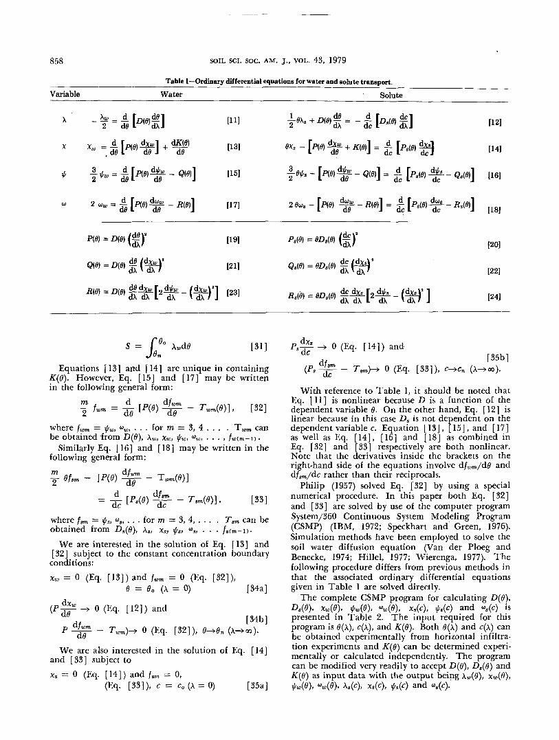
Fie 5—The 0(fm) and C(fm) relationships. Note that the X data (Fig. 5a) was obtained from the sorption experiments and theX, $, and <o data (Fig. 5b, c, and d, respectively) were calculated using the program of Table 2.

Note that the fwn functions associated with 0 are alllarger than the /sn functions associated with C. Thisis to be expected as the salt front lags behind that ofthe water for both horizontal and vertical infiltration.Also note that the order of magnitude of X, x, $, and <•>for both water and chloride is lO"3, lO"6, lO"8, and10~u respectively. The domination of the leadingterms of the expansions in Eq. [9] and [10] obvious-ly depends upon the choice of time, t, and decreasesas t increases in value.

Simple CSMP programs (available on request) werewritten for Eq. [9] and [10]. Experimental and pre-dicted profiles of the reduced water content © vs. depthz at 19,260 sec are plotted in Fig. 6a. The contributionof the tat2 term to the depth z for both the 0 and Cprofiles averaged about 1.5%. The agreement is goodalthough the experimental data show a slightly deeperpenetration than predicted. The associated experi-mental and predicted profiles of reduced chloride con-centration C vs. depth z at the same time of 19,260 secare plotted in Fig. 6b. Again the agreement is goodalthough in this case the experimental data indicatea deeper penetration of chloride than predicted. Thedifference, however, is not large and can be attributed

to small differences in initial water contents, to smalldifferences in bulk density and to other experimentaldifferences between the columns used for the horizon-tal and vertical infiltration experiments. Note thatwater content profile of Fig. 6a shows a rather sharp,abrupt front whereas the chloride content profile ofFig. 6b reveals a slightly greater dispersed front. Al-though not particularly obvious here, the trend forgreater dispersion of the salt front compared to thatof the water front was confirmed in other experiments(K.B. Laryea, 1979. Solute dispersion in soil. Ph.D.Thesis, University of Guelph, Guelph, Ontario).

CONCLUSIONS

The analysis developed by Smiles et al. (1978) todescribe hydrodynamic dispersion during one-dimen-sional sorption of water by soil has been extended toone-dimensional infiltration. A power series solutionin t1'2 for the concentration in solution has been de-veloped in a manner similar to that developed byPhilip (1957) for the movement of water during infil-tration. A computer program written using CSMP wasdeveloped to solve the associated differential equa-


^u§nen Jf

.. c -cnco - cn

.4 .6-^

t = 19260so PREDICTED• EXPERIMENTAL

<*^

Fig. 6—Experimental (•) and predicted (O) infiltration pro-files of @(z) and C(z).

tions. Experiments with a clay loam soil show goodagreement with the theory.

The approach initiated by Smiles et al. (1978) andextended here to include the gravitational effects en-countered during vertical flow present a new way ofdescribing solute movement under conditions of chang-ing water velocities and water contents. This approachfits more closely the natural conditions found in thefield.

ACKNOWLEDGMENTS

The authors acknowledge the cooperation and support ofthe soil physics group at C.S.I.R.O., Canberra, Australia. Wealso acknowledge the technical expertise of Mr. N. Baumgartner,the assistance of Dr. S. S. Wang of the Institute of ComputerScience and helpful discussions with Dr. B. D. Kay.

APPENDIX

The following procedure parallels very closely the develop-ment by Philip (1957, p. 30-34) and only a brief descriptionis included here. Eq. [8] is rewritten as Eq. [Al] using thenotation of Philip:

DS- +dt T dx/ae K - _ Lr D- i

3c L3x/3c J -The dispersion equation for sorption is given by:

Ddx' __9 ~dT + dx'Jde

= _d_ D,dc Lax'/3c •].

[Al]

[A2]

Equations [Al] and [A2] are comparable to Eq. [3.2] and[3.3] respectively of Philip.

Following Philip's procedure one subtracts Eq. [A2] from[Al], substitutes y = x-x' and obtains:

dy 30 3y 9 dc 3V'W-Dw£-K = KlD-l&&- [A3]

Introduction of the approximation dy/dx = dy/8x' and fol-lowing the procedure outlined by Philip gives:

•$-°&'£-*=*V>.&&> ™which is comparable to Eq. [3.10] of Philip.Use of x' = Xi<* in Eq. [A4] gives:

where

and

, a/ i p ay K _ 1 §_ rp ay,6 dt t P 30 K ~ t dc iF> dc ]>

P = r>(dfl/d\)a

The substitution

reduces Eq. [A5] to:

P. = D. (dc/dX)'.

x = y't~

AX AXo* ~ p de - K = d7 lp- d7 I-

[A5]

[A6]

[A7]

[A8]

[A9]

which is Eq. [14] of this text.The second and higher approximations are obtained by fol-

lowing the procedure of Philip as modified for this situation.The results for Q. and R, are given by Eq. [22] and [24] andthe associated differential equations are given by Eq. [16] and[18] respectively.

hydrodynamic dispersion during infiltration of water into soil1

Documents