hydraulic characteristics analysis of an an aerobic ... · invited review paper hydraulic...

891

†To whom correspondence should be addressed.

E-mail: [email protected], [email protected]

Korean J. Chem. Eng., 29(7), 891-902 (2012)DOI: 10.1007/s11814-011-0269-0

INVITED REVIEW PAPER

Hydraulic characteristics analysis of an anaerobic rotatory biological contactor (AnRBC) using tracer experiments and response surface methodology (RSM)

Yadollah Mansouri*, Ali Akbar Zinatizadeh**,†, Parviz Mohammadi***, Mohsen Irandoust****,

Aazam Akhbari****,*****, and Reza Davoodi******

*Young Researchers Club, Ilam Branch, Islamic Azad University, Ilam, Iran**Water and Wastewater Research Center (WWRC), Department of Applied Chemistry,

Faculty of Chemistry, Razi University, Kermanshah, Iran***Department of Environmental Health Engineering, Kermanshah Health Research Center (KHRC),

Kermanshah University of Medical Sciences, Kermanshah, Iran****Department of Analytical Chemistry, Faculty of Chemistry, Razi University, Kermanshah, Iran

*****Sama Technical and Vocatinal Training College, Islamic Azad University, Kermanshah Branch, Kermanshah, Iran******Kermanshah Water and Wastewater Company, Kermanshah, Iran

(Received 19 June 2011 • accepted 15 October)

Abstract−The hydraulic characteristic of an anaerobic rotating biological contactor (AnRBC) were studied by changing

two important hydraulic factors effective in the treatment performance: the hydraulic retention time (τ) and rotational

disk velocity (ω). The reactor hydraulic performance was analyzed by studying hydraulic residence time distribu-

tions (RTD) obtained from tracer (Rhodamine B) experiments. The experiments were conducted based on a central

composite face-centered design (CCFD) and analyzed using response surface methodology (RSM). The region of ex-

ploration for the process was taken as the area enclosed by τ (60, 90 and 120 min) and ω (0.8 and 16 rpm) boundaries.

Four dependent parameters, deviation from ideal retention time (∆τ), dead volume percentage and dispersion indexes

(Morrill dispersion index (MDI) and dispersion number (d)), were computed as response. The maximum modeled ∆τ

and dead volume percentage was 43.03 min and 37.51% at τ and ω 120 min and 0 rpm, respectively. While, the min-

imum predicted responses (2.57 min and 8.08%) were obtained at τ and ω 60 min and 16 rpm, respectively. The inter-

action showed that disk rotational velocity and hydraulic retention time played an important role in MDI in the reactor.

The AnRBC hydraulic regime was classified as moderate and high dispersion (d=0.09 to 0.253). As a result, in addition

to the factors studied, the reactor geometry showed significant effect on the hydraulic regime.

Key words: Anaerobic Rotatory Biological Contactor, Hydraulic Characteristics, Tracer Experiment, Response Surface

Methodology

INTRODUCTION

The hydraulic behavior in biological reactors is of fundamental

importance for the efficiency of wastewater treatment processes.

Examples of hydraulic phenomena with adverse impacts on the bio-

reactors performance include short circuiting streams and dead vol-

umes. The unfavorable hydraulic situations in the bioreactors may

cause lower process performance and thus higher residual concentra-

tions in the treated water. This may be particularly significant in high

loaded bioreactors and anaerobic RBC reactors [1,2]. Owing to a lack

of appreciation for the hydraulics of reactors, many of the treatment

plants that have been built do not perform hydraulically as designed.

Comparison of actual hydraulic characteristics of a reactor measured

using tracers, to the expected theoretical response can be used to

assess the degree to which the ideal design has been achieved [2,3].

Anaerobic rotating biological contactors (AnRBCs) offer an alter-

native treatment technology to the conventional anaerobic digester.

Because of the widespread use of RBCs in recent years, and be-

cause the reactor hydraulics directly affects the treatment perfor-

mance, determination of hydraulic characteristic is of great impor-

tance. Poor hydraulic conditions reduce the HRT and effective vol-

ume, resulting in lower removal efficiencies of the bioreactor. The

presence of a good design model for the RBC reactor is a useful

tool for describing and predicting the RBC hydraulic regime [4-6].

There are several examples of tracer tests being used to indicate

the presence of short circuiting streams and dead volume in differ-

ent reactors. Hydraulic characterization is performed by a retention

time distribution (RTD) curve [7-11]. Not many tracer studies have

been done on the hydraulic characteristics of the RBC reactor, but

a few quantitative models have been proposed [12-16]. In all these

models, there is no common agreement on whether an RBC behaves

as a plug-flow or a completely mixed reactor. Various indexes have

been used to describe the mixing and hydraulic flow pattern in the

different operational units. These are Morrill (MDI), Peclet, disper-

sion (d) numbers etc [1-3]. Non-ideal flow models such as the tank-

in-series (TIS) model and dispersion plug flow (DPF) model are

used to describe the hydraulic flow pattern of an anaerobic baffled

reactor (ABR) [17].

Today, improvements in computer and computational technology

and the development of a new generation of highly efficient com-

puter programs like computational fluid dynamic (CFD) analysis

892 Y. Mansouri et al.

July, 2012

have made it possible to show the inside dynamic flow situation in

structures such as clarifiers and activated sludge reactors [18,19].

Response surface methodology (RSM) is a collection of statistical

and mathematical techniques useful for the process modeling and

optimizing. This methodology is more practical compared to the

other approaches as it arises from experimental methodology, which

includes interactive effects among the variables and, eventually, it

depicts the overall effects of the parameters on the process [20].

In an earlier work published elsewhere [21], we found that low

hydraulic retention time (τ) and disk rotational velocity (ω) had an

adverse impact on the process performance. Hence, in the present

study, in order to explore the best operational conditions achieving

a high hydraulic performance in an anaerobic RBC, the interactions

among two effective variables (τ, ω) as well as their direct impacts

on the hydraulic regime of the AnRBC were investigated. The re-

sponses (deviation from ideal retention time (∆τ), volume of dead

space and dispersion indexes (MDI and d)) were determined using

the data obtained from the tracer experiments, and the hydraulic

characteristics were analyzed and modeled by RSM.

MATERIALS AND METHODS

1. Bioreactor Configuration

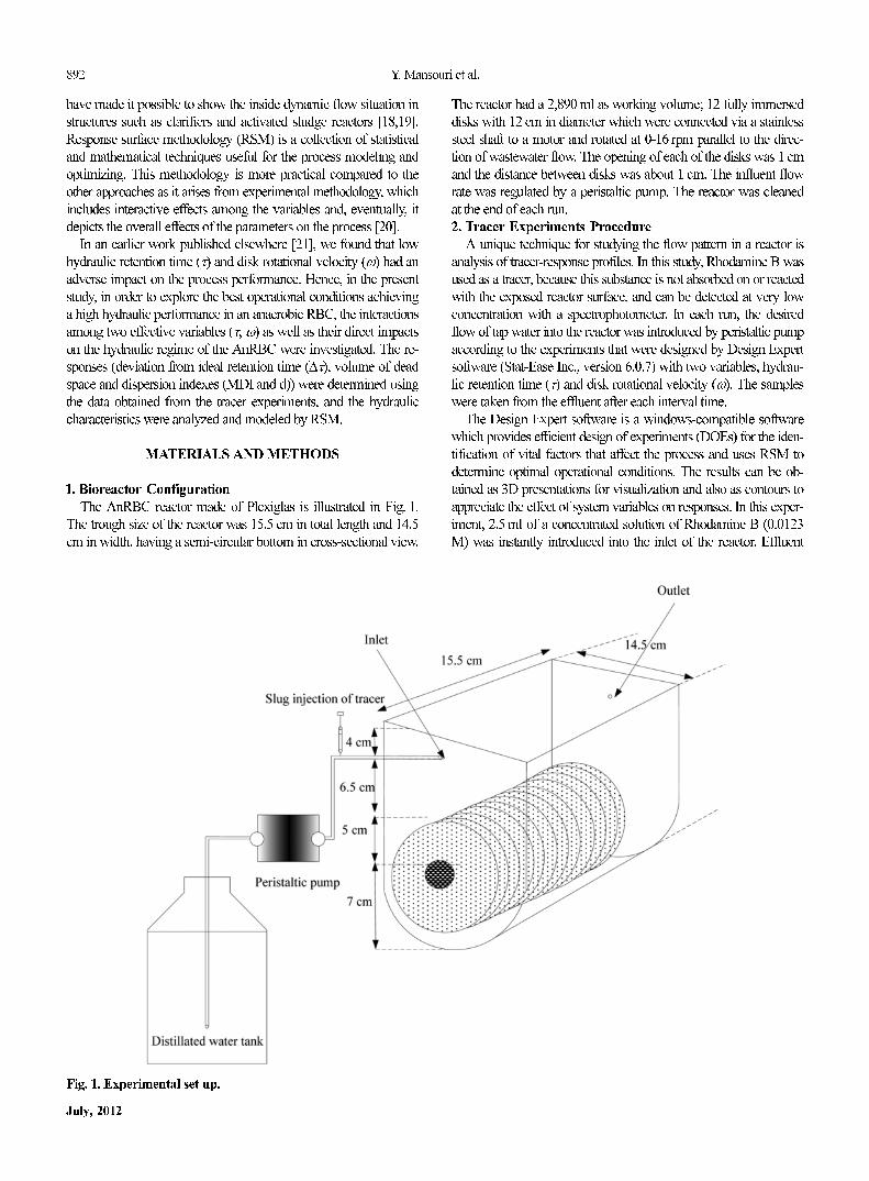
The AnRBC reactor made of Plexiglas is illustrated in Fig. 1.

The trough size of the reactor was 15.5 cm in total length and 14.5

cm in width, having a semi-circular bottom in cross-sectional view.

The reactor had a 2,890 ml as working volume; 12 fully immersed

disks with 12 cm in diameter which were connected via a stainless

steel shaft to a motor and rotated at 0-16 rpm parallel to the direc-

tion of wastewater flow. The opening of each of the disks was 1 cm

and the distance between disks was about 1 cm. The influent flow

rate was regulated by a peristaltic pump. The reactor was cleaned

at the end of each run.

2. Tracer Experiments Procedure

A unique technique for studying the flow pattern in a reactor is

analysis of tracer-response profiles. In this study, Rhodamine B was

used as a tracer, because this substance is not absorbed on or reacted

with the exposed reactor surface, and can be detected at very low

concentration with a spectrophotometer. In each run, the desired

flow of tap water into the reactor was introduced by peristaltic pump

according to the experiments that were designed by Design Expert

software (Stat-Ease Inc., version 6.0.7) with two variables, hydrau-

lic retention time (τ) and disk rotational velocity (ω). The samples

were taken from the effluent after each interval time.

The Design Expert software is a windows-compatible software

which provides efficient design of experiments (DOEs) for the iden-

tification of vital factors that affect the process and uses RSM to

determine optimal operational conditions. The results can be ob-

tained as 3D presentations for visualization and also as contours to

appreciate the effect of system variables on responses. In this exper-

iment, 2.5 ml of a concentrated solution of Rhodamine B (0.0123

M) was instantly introduced into the inlet of the reactor. Effluent

Fig. 1. Experimental set up.

Hydraulic characteristics analysis of an AnRBC using tracer experiments and RSM 893

Korean J. Chem. Eng.(Vol. 29, No. 7)

samples were collected immediately after the observation of the

tracer in the effluent at every 5 min or at lesser time intervals and

tested by spectrophotometer. The operation was continued until no

tracer was detected for at least 2 or 3 times of HRT.

Absorption spectra of Rhodamine B (2×10−4 M) were obtained in

the range of 400-630 nm (Fig. 2(a)). Maximum absorption appeared

at 554 nm at room temperature with UV-visible spectrophotometer

(Agilent 8453, Germany). This maximum absorption was used

throughout the experiments. Fig. 2(b) shows the calibration curve

obtained for Rhodamine B at its respective absorbance λmax (554

nm) with correlation coefficient value of 0.999.

3. Experimental Design

Three important hydraulic factors that influence the treatment

performance of a RBC reactor are hydraulic retention time (τ), disk

rotational velocity (ω) and degree of submergence. The latter vari-

able is eliminated for anaerobic RBC as the disks were fully sub-

merged in the system. In this study, τ and ω were therefore chosen

as the independent and most critical operating factors on the hydrau-

lic regime. The region of exploration for hydraulic regime in the

AnRBC reactor was decided as the area enclosed by τ (60, 120 min)

and ω (0, 16 rpm) boundaries (Table 1). Selection of the range of the

ω was based on the results obtained from the earlier studies [22,23].

The operating conditions as well as their standard deviations are

presented in Table 2, indicative of good agreement between the de-

signed and actual values.

The statistical method of factorial design of experiments (DOE)

eliminates systematic errors with an estimate of the experimental

error and minimizes the number of the experiments [24]. In this

study, as no reaction occurs and both variables and responses are

inherently hydraulic parameters, the face-centered design with the

minimum levels was proposed. In the face-centered design, the axial

points occur at the center of each face of the factorial space, rather

than outside the faces as in the case of a spherical region, so α=±1.

This design requires three levels of each factor. In addition, another

reason for selecting face-centered design in this study was that the

effects of the variables on the responses in the values between the

range studied (−1 to +1) had not shown any unknown curvature in

the literatures as well as in our preliminary study, meaning that it

does not affect the obtained trend. Therefore, the RSM used in the

present study was a central composite face-centered design (CCFD)

involving two different factors, τ and ω.

The hydraulic regime of the AnRBC reactor was assessed based

on the full face-centered CCD experimental plan (Table 3). The de-

sign consisted of 2k factorial points augmented by 2k axial points

and a center point where k is the number of variables. The two op-

erating variables were considered at three levels namely, low (−1),

central (0) and high (1). Accordingly, 13 experiments were conducted

with nine experiments organized in a factorial design (including

four factorial points, four axial points and one center point) and the

Fig. 2. (a) Absorption spectra of 2×10−4 M Rhodamine B, (b) Cali-bration graph for determination of Rhodamine B at its re-spective absorbance (λ

max=554 nm).

Table 2. Standard deviation of operating conditions applied in this study

Factor Designed value in DOERange of measured value

during experimentStandard deviation

Hydraulic retention time (τ), min 060 060.84 ±0.092

090 091.75 ±0.148

120 122.46 ±0.113

Disk rotational velocity (ω), rpm 000 0. ±0.000

008 8. ±0.000

016 16.0 ±0.000

Table 1. Experimental range and levels of the independent vari-ables

VariablesRange and levels

−1 0 1

Hydraulic retention time (τ), min 60 90 120

Disk rotational velocity (ω), rpm 00 08 016


July, 2012

remaining four involving the replication of the central point to get

good estimate of experimental error. Repetition experiments were

carried out after other experiments followed by order of runs designed

by DOE as shown in Table 3.

To do a comprehensive analysis on the hydraulic regime, four

dependent parameters were calculated as response. These parame-

ters were deviation from ideal retention time (∆τ), volume of dead

space, Morrill dispersion index (MDI) and dispersion number (d).

The parameters were determined by the following relationships.

(1)

(2)

(3)

(4)

(5)

(6)

(7)

(8)

(9)

(10)

where, C(t) is tracer concentration at time t, mg/l; is mean resi-

dence time, min; E(t) is residence time distribution function; ∆τ is

deviation from ideal retention time, min; MDI as a measure of the

dispersion is Morrill dispersion index; P90 is 90 percentile value from

log-probability plot, %; P10 is 10 percentile value from log-probability

plot, % and F(t) is cumulative residence time distribution function.

After the experiments were conducted, the coefficients of the poly-

nomial model were calculated using the following equation [25]:

(11)

Where i and j are the linear and quadratic coefficients, respectively,

and β is the regression coefficient. Model terms were selected or

rejected based on the P-value with 95% confidence level. The re-

sults were completely analyzed using analysis of variance (ANOVA)

by Design Expert software. Three-dimensional plots and their respec-

tive contour plots were obtained based on the effect of the levels of

the two factors. From these three-dimensional plots, the simulta-

neous interaction of the two factors on the responses was studied.

The experimental conditions and results are shown in Table 3.

RESULTS AND DISCUSSION

1. Tracer Study

The hydraulic performance of the AnRBC reactor was analyzed

by studying water flow patterns or hydraulic residence time distri-

butions (RTD) obtained from the tracer experiments. Fig. 3(a)-(c)

presents the modeled and experimental data curves of the tracer con-

centration versus time distribution at different τ (60, 90 and 120 min)

and ω (0, 8 and 16 rpm). It is clear from the figure that increase in

τ resulted in an increase in deviation from ideal flow pattern, while

E t( ) = C t( )

C t( )dt0

∞

∫-----------------

t = t( )E t( )∆t∑

∆τ = τ − t

Volume of dead space, % = 1− t

τ--

⎝ ⎠⎛ ⎞100

MDI =

P90

P10

------

F t( ) = E t( )dt0

t

∫

σc

2

=

t2

C t( )dt0

∞

∫

C t( )dt0

∞

∫--------------------- − tc( )2

σθ

2

=

σc

2

τ2

----- = 2D

uL------ + 8

D

uL------⎝ ⎠⎛ ⎞

2

pe = uL

D------

d = D

uL------

t

Y = β0 + βiXi + βjXj + βiiXi

2

+ βjjXj

2

+ βijXiXj + …

Table 3. Experimental conditions and results of central composite design

Run

Variables Responses

Factor 1 Factor 2Deviation from

ideal retention timeMDI

Dead volume

percentage

Dispersion

number (d)

Peclet

number

Hydraulic

retention time (τ)

Disk rotational

velocity (ω)

min rpm min - % - -

01 060 16 03.61 64 07.29 0.23 03.9

02 090 16 22.20 51 17.12 0.19 04.2

03 120 16 31.31 30 28.20 0.13 04.9

04 060 00 19.12 26 33.46 0.14 07.1

05 090 08 13.57 26 17.12 0.16 05.2

06 090 08 09.56 29 14.30 0.17 05.1

07 120 00 43.18 36 37.86 0.10 10.0

08 060 08 09.58 44 17.79 0.18 04.9

09 090 08 17.57 23 21.12 0.15 05.4

10 090 08 15.00 35 24.00 0.16 04.9

11 120 08 26.51 26 24.30 0.13 07.7

12 090 08 13.00 20 19.00 0.14 05.4

13 090 00 32.43 56 37.67 0.13 07.7



an increase in disk rotational velocity caused a decrease in the de-

viation. Comparing the results presented in the figures, it can be

seen that the maximum deviation was obtained at τ and ω, respec-

tively, 120 min and 0 rpm, whereas, the minimum value of the de-

viation was obtained at minimum τ (60 min) and ω (0 rpm). As de-

picted in Fig. 3, high volume of the tracer arrives at the outlet before

mixing with bulk of the liquid in the reactor as disk rotational velocity

equals zero. It was due to the short-cut phenomenon that occurred

which originated from the reactor geometry, inlet and outlet design

and inadequate mixing. From the viewpoint of hydraulic operation,

the values of τ and ω, respectively, 60 min and 16 rpm were advis-

able since they corresponded to the lowest deviation detected.

In general, the RTD curve shows a discrepancy between the mean

residence time and the theoretical residence time. However, it is

possible that stagnate hydraulic zones exist near the inlet or between

the disk, where the tracer can be trapped and slowly released. It must

be noted that, in this reactor, the liquid volume between the disks is

60% of the total liquid volume. Furthermore, the small space be-

tween the disks (1 cm) can hinder the tracer flow, resulting in high

dead volumes for some conditions of τ.

2. Hydraulic Performance Analysis

2-1. Statistical Analysis

The ANOVA results for all responses are summarized in Table 4.

As various responses were investigated in this study, different degree

polynomial models were used for data fitting (Table 4). To quantify

the curvature effects, the data from the experimental results were

fitted to higher degree polynomial equations (i.e., quadratic model).

In the Design Expert software, the response data were analyzed by

default. The model terms in the equations are those remained after

the elimination of insignificant variables and their interactions. Based

on the statistical analysis, the models were highly significant with

very low probability values (from 0.019<0.0001). It is shown that

the model terms of independent variables were significant at 99%

confidence level. The square of correlation coefficient for each re-

sponse was computed as the coefficient of determination (R2). It

showed high significant regression at 95% confidence level. The

value of the adjusted determination coefficient (adjusted R2) was

also high to prove the high significance of the model [25].

The model’s adequacy was tested through lack-of-fit F-tests [26].

The lack of fit results were not statistically significant as the P values

were found to be greater than 0.05. Adequate precision is a meas-

ure of the range in predicted response relative to its associated error

or, in other words, a signal to noise ratio. Its desired value is 4 or

more (26). The value was found to be desirable for all models. Si-

multaneously, low values of the coefficient of variation (CV) (13.39-

17.75%) indicated good precision and reliability of the experiments

as suggested by [25,28]. Detailed analysis of the models is pre-

sented in the following sections.

2-2. Deviation from Ideal Retention Time (∆τ)

Deviation from the ideal retention time (∆τ) can be caused by

channeling and/or recycling of fluid, short circuiting, creation of

stagnant regions in the vessel, and etc. In short circuiting, a portion

of the flow that enters the reactor during a given time period arrives

at the outlet before the bulk of the flow that enters the reactor dur-

ing the same time period arrives. The non ideal flow (short circuit-

ing) can be caused by density currents (due to temperature differ-

ence), wind-driven circulation patterns, inadequate mixing and poor

Fig. 3. Mathematical and empirical curves of tracer concentrationtime distribution for (a) τ=60 min, (b) τ=90 min, (c) τ=120 min.

Table 4. ANOVA results for the equations of the design expert 6.0.6 for studied responses

ResponseThe models selected to

describe the responsesProbability R2 Adj. R2

Adeq.

precisionSD CV PRESS

Probability

for lack of fit

Deviation from ideal retention time Modified quadratic model <0.0001 0.927 0.903 20.67 3.45 17.75 0228.38 0.315

MDI Modified quadratic model <0.0190 0.651 0.536 07.65 9.39 26.20 2705.80 0.103

Dead volume percentage Modified quadratic model <0.0001 0.925 0.888 15.38 4.08 13.39 0189.97 0.815

Dispersion number Modified quadratic model <0.0001 0.970 0.96 33.34 8.70 04.81 0001.97 0.377

R2: determination coefficient, Adj. R2: adjusted R2, Adeq. Precision: adequate precision, SD: standard deviation, CV: coefficient of variation,

PRESS: predicted residual error sum of squares


July, 2012

design. Ultimately, the incomplete use of the reactor volume due to

the above reasons can result in increased ∆τ and reduced treatment

performance.

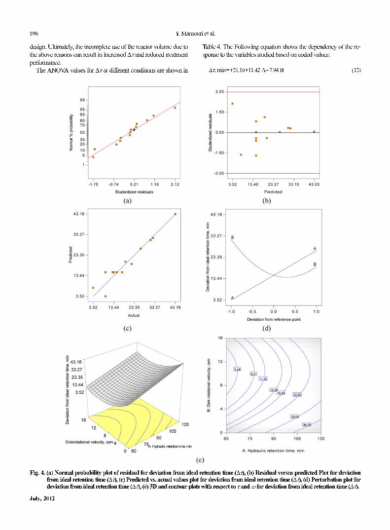
The ANOVA values for ∆τ at different conditions are shown in

Table 4. The Following equation shows the dependency of the re-

sponse to the variables studied based on coded values:

∆τ, min=+21.16+11.42 A−7.94 B (12)

Fig. 4. (a) Normal probability plot of residual for deviation from ideal retention time (∆τ), (b) Residual versus predicted Plot for deviationfrom ideal retention time (∆τ), (c) Predicted vs. actual values plot for deviation from ideal retention time (∆τ), (d) Perturbation plot fordeviation from ideal retention time (∆τ), (e) 3D and contour plots with respect to τ and ω for deviation from ideal retention time (∆τ).



From the equation, the main effect of A and B was significant model

terms. ANOVA results of these quadratic models presented in Table 4

indicate that the above equation could be used to navigate the design

space. Fig. 4(a) displays the normal probability of the residuals, to

verify whether the standard deviations between the actual and the

predicted responses values do follow the normal distribution. The

general impression from the Fig. 4(a) reveals that the underlying

errors were distributed normally as the residuals fall near to a straight

line, and thus, there is no severe indication of non-normality of the

experimental results.

The plots of the residuals versus predicted response are pre-

sented in Fig. 4(b). The general impression is that the plot should

be a random scatter, suggesting that the variance of original obser-

vations is constant for all values of the response. If the variance of

the response depends on the mean level of the response, then this

plot often exhibits a funnel-shaped pattern [26,29,30]. This is also

an indication that there was no need for transformation of the re-

sponse variable. As depicted in the Fig. 4(b) all points of experi-

mental runs were scattered randomly within the constant range of

residuals across the graph, i.e., within the horizontal lines at point

of ±3.0. This implies that the model proposed is adequate and the

constant variance assumption was confirmed.

The actual and the predicted plot for ∆τ are shown in Fig. 4(c).

In the figure the values of R2 and R2adj were evaluated as 0.93 and

0.90, respectively. The perturbation plot (Fig. 4(d)) shows the com-

parative effects of all variables on the response. It is clear from this

figure that the response was very sensitive to both variables (τ and ω).

Fig. 4(e) depicts 3D and contour plots for ∆τ with respect to the

two variables (τ and ω) in the studied design space. From the re-

sults, the two factors were found to be influential in the response as

confirmed in the perturbation plot (Fig. 4(e)). As noted in Fig. 4(d)

and (e), increasing in the ô resulted in an increase in the response,

while the reverse effect was caused by increasing the disk rotational

velocity. This is proved in the model with positive and negative co-

efficients. From Fig. 4(e), an increase in ω from 0 to 8 rpm caused

a remarkable decrease in ∆τ, whereas further increase in ω did not

show any significant effect on the response. It was attributed to the

relatively high volume of the liquid over the disks that creates dead

space, so that the energy supplied by the disks rotation was not suf-

ficient for eliminating the effects of the spaces. The maximum value

of the modeled ∆τ was 43.03 min at τ and ω, 120 min and 0 rpm,

respectively. Whereas, the minimum predicted response (2.57 min)

was obtained at τ and ω 60 min and 16 rpm, respectively. High value

of ∆τ at low disk rotational velocity (as shown in the Fig. 4(e)) re-

sulted in inadequate mixing as well as poor design of this reactor.

Without sufficient energy input, portions of the reactor contents may

not mix with the incoming water; also, because of the poor design of

the reactor (close and opposite inlet and outlet), dead zones develop

within the reactor that will not mix with the incoming water or short

circuiting occurs.

2-3. Dead Volume Percentage

To elucidate the ∆τ, the dead zone volume was also studied as a

response. Dead space can be categorized into hydraulic dead space

and biological dead space. Hydraulic dead space is a function of

flow rate and the number of disks in the reactor, while biological

dead space is a function of the biomass concentration and activity.

However, the hydraulic dead space is the major contributor to the

dead space of AnRBC, especially in treating low strength waste-

water because the biological dead space resulting from gas flow

velocity and diffusion of the tracer into biofilm is neglected (due to

the tin biofilm formed on the discs).

ANOVA results for dead volume are shown in Table 4. As it is

noted in the table, a quadratic model was fitted with the experi-

mental data. The quadratic model shows that the main effect of τ

(A), ω (B), two-level interaction (AB) and second order effects of

B2 are significant model terms in the response. Other model term,

A2, is not significant (with a probability value larger than 0.05). There-

fore, this model term was excluded from the study to improve the

model. The following regression equation is the empirical model

in terms of the coded factors for dead volume percentage.

Dead volume, %=+19.66+5.30A−9.40 B+7.27 B2+4.13 AB (13)

The major diagnostic plots in Figs. 5(a)-(d) are used to determine

the residual analysis of response surface design, ensuring that the

statistical assumptions fit the analysis data. The results obtained from

diagnostic plots and ANOVA results showed that values of dead

volume percentage from the model and the actual experimental data

were in good agreement. The predicted versus actual plot for the

response is in Fig. 5(c), which shows that the actual values are dis-

tributed relatively close to the straight line (y=x). The perturbation

plot (Fig. 5(d)) shows the comparative effects of τ and ω on the re-

sponse. From the results, more significant factors on dead volume

were found to be disk rotational velocity (with similar trend as dem-

onstrated in Fig. 4(d) and e for

∆τ). Fig. 5(e) presents 3D and contour

plots of the modified quadratic model for variation in the volume of

dead space, as a function of τ (A) and ω (B). In the figure the re-

sponse increased upon increasing the τ and decreasing the ω. The

worst condition was obtained for τ=120 min and ω=0, which is

explained by the inadequate mixing and low flow rate. For the ex-

periments of hydraulic retention time 60 and 90 min in ω=0 the

detected dead volume was also very high. The maximum response

observed was 37.86% at τ and ω of 2 h and 1 rpm, respectively.

While, the minimum predicted response (8.08%) was obtained at τ

and ω of 1 h and 16 rpm, respectively.

2-4. Dispersion Indexes

2-4-1. Morrill Dispersion Index (MDI)

One important factor that indicates the type of the reactor (com-

plete mix or plug-flow) is the Morrill dispersion index (MDI). MDI

can be used as a diagnostic tool for ascertaining the features of flow

patterns in reactors. These include the possibilities of bypassing and/

or regions of stagnant fluid (i.e., dead space). A ratio of 90 to 10

percent values from the cumulative tracer curve (Fig. 3) could be

used as a measure of the dispersion index. The value for an ideal

plug-flow reactor is 1.0 and about 22 and more for complete-mix

reactors. MDI was computed for different operational conditions

studied.

The ANOVA results for MDI are shown in Table 4. From the

analysis, A, AB and B2 are significant model terms. Insignificant

model terms were found to be B and A2 that were excluded from

the model to improve the model.

MDI=+29.03−7.03A+14.77B2−11.00AB (14)

The predicted versus actual plot for MDI is shown in Fig. 6. While

the R2 value of the modified quadratic model (R2=0.65) is not as


July, 2012

high as that of the models for the other responses, it nevertheless,

shows a reasonable degree of correlation between the parameters

(Fig. 6). Fig. 7 shows the response surface and contour plots of the

quadratic model for MDI with respect to τ (A) and ω (B) within

the design space. As can be seen in the Fig. 7, the most significant

factor on MDI was determined to be ω. A reverse impact of increas-

ing disk rotational velocity on MDI was observed as the variable

increased (Fig. 7). At low τ (corresponding to high flow rate), an

increase in disk rotational velocity (from 0 to 8) caused a decrease

in the response. Whereas, at higher ω (from 8 to 16) an increase in

Fig. 5. (a) Normal probability plot of residual for Dead volume percentage, (b) Residual versus predicted Plot for Dead volume percentage,(c) Predicted vs. actual values plot for Dead volume percentage, (d) Perturbation plot for Dead volume percentage, (e) 3D andcontour plots with respect to τ and ω for Dead volume percentage.



the variable increased the response.

Decreasing in τ and increasing in ω together leads the hydraulic

regime to complete mixing, which is identified by the higher values

of MDI. From the results shown in Fig. 7, the aforementioned prin-

ciple is confirmed except for the data obtained at the conditions with

no mechanical mixing (ω=0 rpm). The high value of the MDI in

the lower ω was not a sign of the high value of mixing and disper-

sion. This was because of the short-cut phenomenon that resulted

from the poor reactor geometry and inlet and outlet design. As can

be seen in Fig. 1, inlet and outlet are against each other with 6.5

cm away from the disks, providing about one-third of the reactor

volume in the upper part where adequate mixing is not supplied.

The poor design of the inlet and outlet develops a dead zone within

the reactor. The reason is justified by the normalized residence time

distribution curves shown in the Fig. 7.

To elucidate the residence time distribution of the fluid in the re-

actor, the E(t) and F(t) curves have been shown in corners of Fig.

7. From the E(t) curve, the initial peak at ω=0 (τ=60 and 120 min)

clearly indicates a short circuiting stream. Also, as shown in Eq.

(6), the F(t) curve is the integral of the E(t) curve, while the E(t)

curve represents the amount of the tracer that has remained in the

reactor for less than the time t. As can be observed, E(t) and F(t)

show higher initial values at the lowest ω compared to the values

at the higher ω. So that, at τ=60 min and ω=0, 48% of the fluid

had a residence time of less than 5 minutes, 41% between 5 and

60 minutes and 11% more than 60 minutes. While these values were

obtained 8.34, 57.11 and 34.5%, respectively, at τ=60 min and ω=

16 rpm. For τ=120 and ω=0, the values were 16.05% with τ less

than 10 minutes, 57.53% between 10 and 120 minutes and 26.42%

more than 120 minutes. Whereas, for τ=120 and ω=16, the val-

ues were obtained, respectively, 9.1, 63.97 and 26.93%. The inter-

action showed that disk rotational velocity and τ played an important

role in MDI in the reactor. The maximum MDI was found to be

61.83 at τ and ω of 60 min and 16 rpm respectively.

2-4-2. Dispersion Number

Another important response describing the hydraulic behavior

Fig. 7. Response surface and counter plots for MDI with respect to τ and ω.

Fig. 6. Predicted vs. actual values plot for MDI.


July, 2012

of the AnRBC is the dispersion, which is a measure of the degree

of mixing in the bioreactor. As the dispersion increases, the con-

centration of a certain pollutant decreases and thus leads to higher

removal efficiency. A complementary measure of the dispersion is

the dispersion number, which is defined as the inverted Peclet num-

ber (Eq. (9) and Table 3). To get a meaningful interpretation of the

flow pattern in the AnRBC reactor, the values of dispersion num-

ber in the different conditions as a response were calculated and

displayed in Table 3.

The predicted versus actual plot for the response (Fig. 8(a)) shows

that the actual values are distributed close to the straight line (y=x).

From the ANOVA results (Table4), A, B and A2 are significant model

terms. Insignificant model terms, which have limited influence, such

as AB and B2, were excluded from the study to improve the model.

The following regression equation is the empirical model in terms

of coded factors for dispersion number (d):

Dispersion number (d)=+0.19−0.027A+0.054* B−0.019A2 (15)

The effects of τ and ω on the dispersion number are shown in Fig.

8(b). The most significant factor effective in the response was deter-

mined to be disk rotational velocity (ω). Increase in ω from 0 to

15 min/h resulted in an increase in dispersion number with a main

order effect, while with increase in τ the response was decreased.

The perturbation plot shown in Fig. 8(c) demonstrates the compar-

ative effects of τ and ω on the response. An increasing linear slope in

ω and decreasing curvature of τ shows that the response was sensi-

tive to these two process variables with different effects.

The maximum and minimum dispersion number was obtained

0.253 and 0.09 at τ and ω of 60 min, 16 rpm and 120 min, 0 rpm,

respectively. However, for practical purposes, the following disper-

sion values can be used to assess the degree of axial dispersion in

wastewater treatment facilities [3].

Fig. 8. (a) Predicted vs. actual values plot for dispersion number, (b) 3D plot with respect to τ and ω for Dispersion number, (c) Perturbationplot for dispersion number.



No dispersion d=0 (ideal plug flow)

low dispersion d≤0.05

Moderate dispersion d=0.05-0.025

High dispersion d≥0.25

Based on the computed values of the dispersion number (0.09

to 0.253) and above discussion, the AnRBC hydraulic regime is

classified as moderate and high dispersion. At low disk rotational

velocity and higher hydraulic retention time, the values of d were

observed to be low. In contrast, at high disk rotational speeds, high

d was obtained. Hence, it may be stated that, in a majority of flow

situations, an AnRBC reactor behaves more like a complete mix

regime with axial dispersion rather than being a plug flow one.

CONCLUSION

The hydraulic characteristics of the AnRBC reactor at various

levels of hydraulic retention time (τ) and disk rotational velocity

(ω) were constructively investigated. This study showed that in addi-

tion to the factors studied, reactor geometry had a significant effect

on the hydraulic regime. Improving the reactor design (modifying

inlet and outlet structure, eliminating the dead volume, etc.) can avoid

high energy consumption supplied by the disk rotation or influent

flow rate that is strongly advised for scale-up stage. However, the

following salient points were obtained.

• τ and ω were found to be influential for the deviation from

ideal retention time (∆τ). Increasing τ resulted an increase in ∆τ,

while the reverse effect was caused by increasing the disk rotational

velocity. The volume of dead space increased upon increasing the

τ and decreasing the ω.

• Based on the computed values of the dispersion number (0.09

to 0.253), the AnRBC hydraulic regime is classified as moderate

and high dispersion. In the majority of flow situations, the AnRBC

reactor behaved more like a complete mix regime with axial disper-

sion rather than being a plug flow one.

• Most significant factor on MDI was ω. At low HRTs (corre-

sponding to high flow rate), an increase in disk rotational velocity

(from 0 to 8) caused a decrease in the response. While at higher

rpm (from 8 to 16), an increase in the variable increased the response.

The maximum MDI was found to be 61.83 at τ and ω of 60 min

and 16 rpm, respectively.

ACKNOWLEDGEMENT

The financial support provided by Kermanshah Water and Waste-

water Company is gratefully acknowledged. The authors acknowledge

the laboratory equipment provided by the Water and Power Industry

Institute for Applied and Scientific Higher Education (Mojtama-e-

gharb), Kermanshah that has resulted in this article. The authors also

wish to thank Mrs S. Kiani for her assistance (Technical Assistant

of Water and Wastewater Laboratory).

NOMENCLATURE

AnRBC : anaerobic rotating biological contactor

CCD : face-centered design

CCFD : central composite face-centered design

CFD : computational fluid dynamic

C(t) : tracer concentration at time t [mg/l]

CV : coefficient of variation

D : coefficient of axial dispersion [m2/s]

d : dispersion number

DoE : design of experiment

E(t) : residence time distribution function

F(t) : cumulative residence time distribution function

i : linear coefficient

j : quadratic coefficient

k : number of variables

L : characteristic length [m]

MDI : morrill dispersion index

P90 : 90 percentile value from log-probability plot [%]

P10 : 10 percentile value from log-probability plot [%]

Pe

: peclet number

RSM : response surface methodology

RTD : retention time distribution

u : fluid velocity [m/s]

∆τ : deviation from ideal retention time [min]

β : regression coefficient

: mean residence time [min]

σc

2 : variance of normalized tracer response [s2]

σ θ

2 : variance derived from C curve [s2]

ω : rotational disk velocity

τ : hydraulic retention time

REFERENCES

1. O. Levenspiel, Chemical reactor engineering, 2nd Ed., Wiley, New

York (2000).

2. H. Fogler Scott, Elements of chemical reaction engineering, 3rd Ed.,

Prentice Hall PTR (2001).

3. Metcalf & Eddy, Wastewater engineering, 4th Ed., McGraw Hill,

New York (2003).

4. T. Yamaguch, I M.T., shida Suzuki, J. Process Biochem., 35, 403

(1999).

5. F. Kargi and S. Eker, J. Enzyme Microb. Technol., 32, 464 (2003).

6. G. D. Najafpour, A. A. L. Zinatizadeh and L. K. Lee, J. Biochem.

Eng., 30, 297 (2006).

7. H. Bode and C. Seyfried, J. Water Sci. Technol., 17, 197 (1984).

8. B. Newell, J. Bailey, A. Islam, L. Hopkins and P. Lant, J. Water Sci.

Technol., 37, 43 (1998).

9. S. C. Williams and J. Beresford, J. Water Sci. Technol., 38 55 (1998).

10. L. J. Burrows, A. J. Stokes, A. D. West and C. F. Martin, J. Water

Res., 33, 367 (1999).

11. A. D. Martin, J. Chem. Eng. Sci., 55, 5907 (2000).

12. B. H. Kornegay and J. F. Andrews, J. WPCF, 460 (1968).

13. J. H. Clark, E. M. Moneg and T. Asano, J. WPCF, 896 (1978).

14. Y. C. Wu and E. D. Smith, J. Environ. Eng. Div., (Proc. ASCE) 108

(1982).

15. K. P. Hsueh, O. J. Hao and Y. C. Wu, J. WPCF, 63, 67 (1991).

16. G. Banerjee, J. Water Res., 31, 2500 (1997).

17. Y. Saratha1, T. Koottatep and A. Morel, J. Environ. Scien., 22, 1319

(2010).

18. A. B. Karama, O. O. Onyejekwe, C. J. Brouckaert and C. A. Buck-

ley, J. Water Sci. Technol., 39, 329 (1999).

19. J. Zhang, P. M. Huck and W. B. Anderson, Optimization of a full-

t


July, 2012

scale ozone disinfection process based on computational fluid

dynamics analysis, in 11th gothenburg symposium, Chemical Water

and Wastewater Treatment VIII. Orlando, Florida, USA (2004).

20. D. Bas and B. I. H. Oyaci, J. Food Eng., 78, 836 (2007).

21. A. Akhbari, A. A. Zinatizadeh, P. Mohammadi, M. Irandoust and

Y. Mansouri, J. Chem. Eng., 168, 269 (2011).

22. L. D. Palma, C. Merli, M. Paris and E. Petrucci, J. Bioresour.,

(2003).

23. A. Tawfik, A. Klapwijk, F. El-Gohary and G. Lettinga, J. Biochem.

Eng., 25, 89 (2005).

24. R. Kuehl, Design of Experiments: Statistical principles of research

design and analysis, 2nd Ed., C.A: Duxbury Press (2000).

25. A. I. Khuri and J. A. Cornell, Response surfaces: Design and anal-

yses, 2nd Ed., Marcel Dekker, New York (1996).

26. D. C. Montgomery, Design and analysis of experiments, 3rd Ed.,

Wiley, NewYork (1991).

27. R. L. Mason, R. F. Gunst and J. L. Hess, Statistical design and analy-

sis of experiments, eighth applications to engineering and science,

2nd Ed., Wiley, New York (2003).

28. A. L. Ahmad, S. Ismail and S. Bhatia, J. Environ. Sci. Technol., 39,

2828 (2005).

29. R. H. Myers and D. C. Montgomery, Response surface methodol-

ogy: Process and product optimization using designed experiments,

2nd Ed., Wiley, New York (2002).

30. D. C. Montgomery, Design and analysis of experiments, 4th Ed.,

Wiley, New York (1996).

hydraulic characteristics analysis of an an aerobic ... · invited review paper hydraulic...

Documents