hybrid systems biology: application to escherichia coli · hybrid systems biology: application to...
TRANSCRIPT
Rui Miguel Correia Portela
Graduated in Molecular and Cell Biology
Hybrid Systems Biology: Application to
Escherichia coli
Dissertation presented to obtain a Master degree in Biotechnology
Supervisor: Rui Oliveira, Professor Auxiliar, FCT-UNL
Jury:
President: Prof. Doutor Pedro Miguel Ribeiro Viana Baptista
Examiner: Prof. Doutor João Montargil Aires de Sousa
September 2011

II

III
Hybrid Systems Biology: Application to Escherichia coli
Copyright Rui Miguel Correia Portela, FCT/UNL, UNL
A Faculdade de Ciências e Tecnologia e a Universidade Nova de Lisboa têm o direito,
perpétuo e sem limites geográficos, de arquivar e publicar esta dissertação através de exemplares
impressos reproduzidos em papel ou de forma digital, ou por qualquer outro meio conhecido ou
que venha a ser inventado, e de a divulgar através de repositórios científicos e de admitir a sua
cópia e distribuição com objectivos educacionais ou de investigação, não comerciais, desde que
seja dado crédito ao autor e editor.
The Faculty of Science and Technology and the New University of Lisbon have the
perpetual right, and without geographical limits, to archive and publish this dissertation through
press copies in paper or digital form, or by other known form or any other that will be invented,
and to divulgate it through scientific repositories and to admit its copy and distribution with
educational or research objectives, non-commercial, as long as it is given credit to the author.

IV

V
Acknowledgements
I owe my deepest gratitude to Prof. Rui Oliveira, for the thesis coordination and support; I
can hardly think of a better way to start my scientific career.
I am also in debt with all the elements of Systems Biology and Engineering group; I hope
to be able to transmit with this thesis the group outstanding working environment.
I would like to show my gratitude to my lunch buddies, who made the days in front of the
pc much easier.
To the entities that funded the research FCT (MIT-Pt/BSBB/0082/2008).
Gostaria de agradecer à minha família, especialmente aos meus pais e tios pelo apoio re-
levado durante todos estes anos.
I would like to thank my family, especially my parents and uncles for the support re-
vealed through all these years.
To all my good friends, those who made this a really special place; Particularly to Tânia
and João, without you those previous four years would be much more difficult.
And last, but anything but least, Marino, who, among many other things, made me enjoy
doing what I like to do.
To all of you,
My deepest and sincere thanks!

VI

VII
Abstract
In complex biological systems, it is unlikely that all relevant cellular functions can be
fully described either by a mechanistic (parametric) or by a statistic (nonparametric) modelling
approach. Quite often, hybrid semiparametric models are the most appropriate to handle such
problems. Hybrid semiparametric systems make simultaneous use of the parametric and
nonparametric systems analysis paradigms to solve complex problems. The main advantage of the
semiparametric over the parametric or nonparametric frameworks lies in that it broadens the
knowledge base that can be used to solve a particular problem, thus avoiding reductionism.
In this M.Sc. thesis, a hybrid modelling method was adopted to describe in silico
Escherichia coli cells. The method consists in a modified projection to latent structures model that
explores elementary flux modes (EFMs) as metabolic network principal components. It
maximizes the covariance between measured fluxome and any input “omic” dataset. Additionally
this method provides the ranking of EFMs in increasing order of explained flux variance and the
identification of correlations between EFMs weighting factors and input variables.
When applied to a subset of E. coli transcriptome, metabolome, proteome and envirome
(and combinations thereof) datasets from different E. coli strains (both wild-type and single gene
knockout strains) the model is able, in general, to make accurate flux predictions. More
particularly, the results show that envirome and the combination of envirome and transcriptome
are the most appropriate datasets to make an accurate flux prediction (with 88.5% and 85.2% of
explained flux variance in the validation partition, respectively). Furthermore, the correlations
between EFMs weighting factors and input variables are consistent with previously described
regulatory patterns, supporting the idea that the regulation of metabolic functions is conserved
among distinct envirome and genotype variants, denoting a high level of modularity of cellular
functions.
Keywords
System Biology; Projection to latent structures; Hybrid methods; Escherichia coli;
Elementary flux modes; Multiple omic analysis

VIII
IX
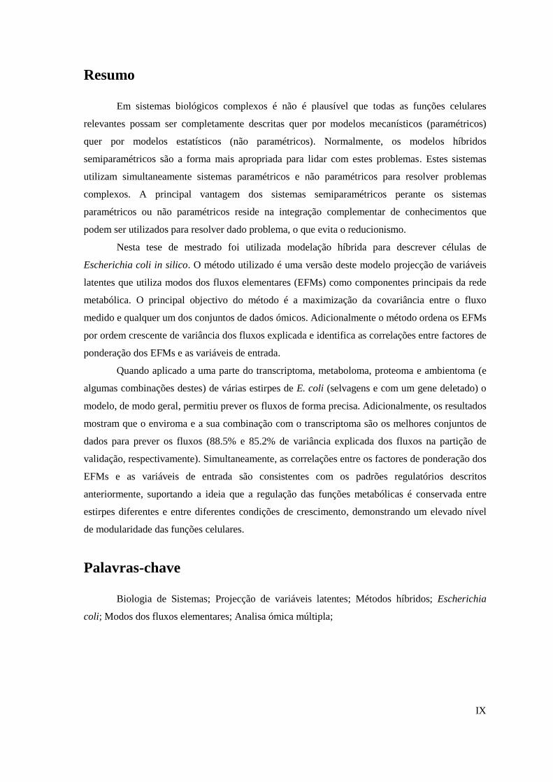
Resumo
Em sistemas biológicos complexos é não é plausível que todas as funções celulares
relevantes possam ser completamente descritas quer por modelos mecanísticos (paramétricos)
quer por modelos estatísticos (não paramétricos). Normalmente, os modelos híbridos
semiparamétricos são a forma mais apropriada para lidar com estes problemas. Estes sistemas
utilizam simultaneamente sistemas paramétricos e não paramétricos para resolver problemas
complexos. A principal vantagem dos sistemas semiparamétricos perante os sistemas
paramétricos ou não paramétricos reside na integração complementar de conhecimentos que
podem ser utilizados para resolver dado problema, o que evita o reducionismo.
Nesta tese de mestrado foi utilizada modelação híbrida para descrever células de
Escherichia coli in silico. O método utilizado é uma versão deste modelo projecção de variáveis
latentes que utiliza modos dos fluxos elementares (EFMs) como componentes principais da rede
metabólica. O principal objectivo do método é a maximização da covariância entre o fluxo
medido e qualquer um dos conjuntos de dados ómicos. Adicionalmente o método ordena os EFMs
por ordem crescente de variância dos fluxos explicada e identifica as correlações entre factores de
ponderação dos EFMs e as variáveis de entrada.
Quando aplicado a uma parte do transcriptoma, metaboloma, proteoma e ambientoma (e
algumas combinações destes) de várias estirpes de E. coli (selvagens e com um gene deletado) o
modelo, de modo geral, permitiu prever os fluxos de forma precisa. Adicionalmente, os resultados
mostram que o enviroma e a sua combinação com o transcriptoma são os melhores conjuntos de
dados para prever os fluxos (88.5% e 85.2% de variância explicada dos fluxos na partição de
validação, respectivamente). Simultaneamente, as correlações entre os factores de ponderação dos
EFMs e as variáveis de entrada são consistentes com os padrões regulatórios descritos
anteriormente, suportando a ideia que a regulação das funções metabólicas é conservada entre
estirpes diferentes e entre diferentes condições de crescimento, demonstrando um elevado nível
de modularidade das funções celulares.
Palavras-chave
Biologia de Sistemas; Projecção de variáveis latentes; Métodos híbridos; Escherichia
coli; Modos dos fluxos elementares; Analisa ómica múltipla;

X
XI
Contents
Abstract ............................................................................................................................ VII
Keywords ......................................................................................................................... VII
Resumo .............................................................................................................................. IX
Palavras-chave ................................................................................................................... IX
List of figures.................................................................................................................. XIII
List of tables .................................................................................................................... XV
List of abbreviations ....................................................................................................... XIX
1 Introduction .................................................................................................................. 1
1.1 Mechanistic models of bionetwork systems ......................................................... 4
1.1.1 Metabolic reaction-oriented network models ................................................. 4
1.1.2 Function oriented models ................................................................................ 5
1.2 Statistical models .................................................................................................. 6
1.3 Hybrid semiparametric models ............................................................................. 7
1.4 Objectives ............................................................................................................. 8
2 Methods ...................................................................................................................... 11
2.1 E. coli data .......................................................................................................... 13
2.2 E. coli metabolic network ................................................................................... 15
2.3 E. coli elementary flux modes ............................................................................ 16
2.4 Statement of the modelling problem .................................................................. 16
2.5 Hybrid modelling method ................................................................................... 18
2.5.1 Statement of the mathematical problem ........................................................ 18
2.5.2 Projection to latent structures ........................................................................ 20
2.5.3 Projection to latent pathways ........................................................................ 21
2.6 Implementation details ....................................................................................... 23
2.6.1 Software ........................................................................................................ 23
2.6.2 Data organization .......................................................................................... 23
2.6.3 Validation and calibration partitions ............................................................. 23
2.6.4 Principal components optimization ............................................................... 24
2.6.5 EFMs feasibility examination ....................................................................... 24
2.6.6 Consistency analysis ..................................................................................... 25
3 Results ........................................................................................................................ 27
3.1 Model structure discrimination ........................................................................... 29
3.1.1 Models with single omic information layers ................................................. 29
3.1.2 Models with multiple omic information layers ............................................. 33

XII
3.2 Envirome as input to PLP .................................................................................. 37
3.2.1 Discriminated EFMs ..................................................................................... 37
3.2.2 Predictive power ........................................................................................... 37
3.2.3 Envirome-to-function relationship ............................................................... 39
3.3 Envirome and transcriptome as input to PLP ..................................................... 40
3.3.1 Discriminated EFMs ..................................................................................... 40
3.3.2 Predictive power ........................................................................................... 40
3.3.3 Relationship between input and cellular function ........................................ 41
4 Discussion .................................................................................................................. 43
4.1 Relevance of omic information for flux-phenotype prediction .......................... 45
4.2 Envirome flux prediction analysis ..................................................................... 46
4.2.1 Discriminated EFMs ..................................................................................... 46
4.2.2 Predictive power ........................................................................................... 47
4.2.3 Envirome function mapping ......................................................................... 48
4.3 Envirome and transcriptome flux prediction analysis ........................................ 50
4.3.1 Discriminated EFMs ..................................................................................... 50
4.3.2 Input data to function relationship ................................................................ 51
5 Conclusions ................................................................................................................ 53
6 References .................................................................................................................. 57
7 Appendix .................................................................................................................... 63
7.1 Appendix A ........................................................................................................ 65
7.2 Appendix B ........................................................................................................ 74
7.3 Appendix C ........................................................................................................ 76
7.4 Appendix D ........................................................................................................ 88
7.5 Appendix E ........................................................................................................ 92

XIII
List of figures
Figure 1.1: The theoretical basis of constraint-based modelling and FBA. a – Without
constraints, the hypothetical flux distribution of a biological network can be set anywhere in the
solution space (any combination of metabolic fluxes). b – When mass balance constraints are
imposed by the stoichiometric matrix S (in 1) and capacity constraints (flux vi lower and upper
bounds ai and bi, respectively – 2) are applied, it is defined a plausible solution space. c – Through
optimization of an objective function Z, FBA identifies a single flux distribution that lies on the
edge of the allowable solution space [11]. ....................................................................................... 4
Figure 2.1: E. coli metabolic network composed by 43 reactions and 24 metabolites.
Bold metabolites represent the ones that can exit the system; these reactions are not explicit
shown in the scheme. Reactions from 32 to 43 represent the exit of G6P, F6P, R5P, E4P, G3P,
3PG, PEP, PYR, AcCoA, OAA, 2-KG and CO2, respectively....................................................... 15
Figure 2.2: Representation of the influence of the genome and the omic in the fluxome
(R). The genome sets the metabolic capabilities of the cell (elementary flux mode – emk). Each
metabolic function is up- or down- regulated by all omic factors (λk). .......................................... 17
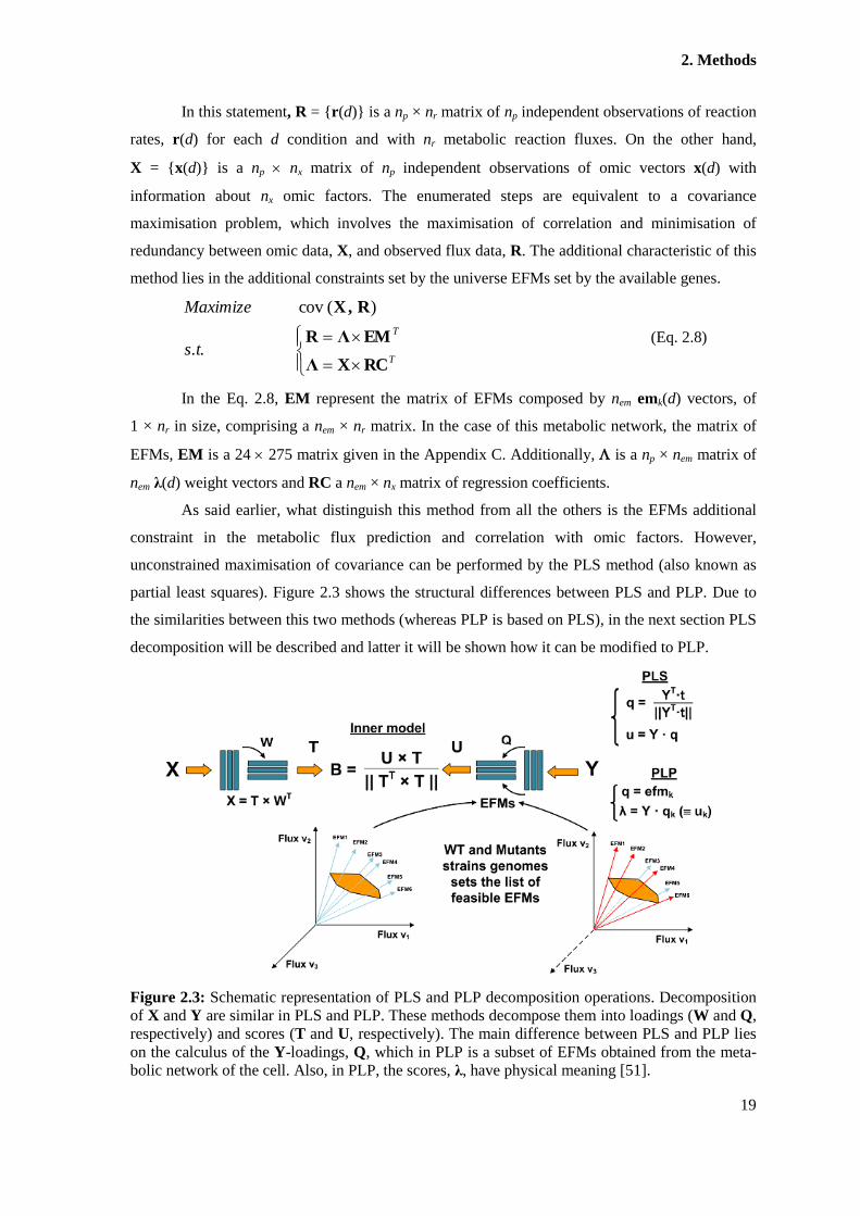
Figure 2.3: Schematic representation of PLS and PLP decomposition operations.
Decomposition of X and Y are similar in PLS and PLP. These methods decompose them into
loadings (W and Q, respectively) and scores (T and U, respectively). The main difference
between PLS and PLP lies on the calculus of the Y-loadings, Q, which in PLP is a subset of
EFMs obtained from the metabolic network of the cell. Also, in PLP, the scores, λ, have physical
meaning [51]. .................................................................................................................................. 19
Figure 3.1: Frequency of selection of each EFM in the bootstrapping validation
procedure when envirome is the input data. ................................................................................... 38
Figure 3.2: Predicted against measured fluxes with envirome as input to PLP for the
calibration partition (blue circles) and validation partition (grey triangles). .................................. 38
Figure 3.3: Measured (blue bar) and predicted (grey bar) metabolic flux for the reference
strain grown at 0.2h-1
as dilution rate (A) and mutant talB (B) both present in validation partition
of PLP algorithm with envirome as input data. .............................................................................. 39
Figure 3.4: Frequency of selection of each EFM in the bootstrapping validation
procedure when envirome and transcriptome are the input data. ................................................... 40
Figure 3.5: Predicted against measured fluxes with proteome and transcriptome as input
to PLP for the calibration partition (blue circles) and validation partition (grey triangles). .......... 41
Figure 3.6: Measured (blue bar) and predicted (grey bar) metabolic flux for the reference
strain grown at 0.2h-1
as dilution rate (A) and mutant talB (B) both present in validation partition
of PLP algorithm with envirome and transcriptome as input data. ................................................ 42

XIV
Figure 3.7: Regression coefficients between the input components (envirome – index 1 to
9 – and transcriptome – index 10 to 94) and selected EFMs ......................................................... 42

XV
List of tables
Table 3.1: Ranking of statistically significant EFMs with high correlation with the
envirome. Each EFM is selected with increasing explained flux variance. It can also be examined
the statistical relevance of each EFM trough the analysis of pvalue and r2 value. ............................ 30
Table 3.2: Ranking of statistically significant EFMs with high correlation with the
proteome. Each EFM is selected with increasing explained flux variance. It can also be examined
the statistical relevance of each EFM trough the analysis of pvalue and r2 value. ............................ 30
Table 3.3: Ranking of statistically significant EFMs with high correlation with the
metabolome. Each EFM is selected with increasing explained flux variance. It can also be
examined the statistical relevance of each EFM trough the analysis of pvalue and r2 value. ........... 31
Table 3.4: Ranking of statistically significant EFMs with high correlation with the
transcriptome. Each EFM is selected with increasing explained flux variance. It can also be
examined the statistical relevance of each EFM trough the analysis of pvalue and r2 value. ........... 32
Table 3.5: Ranking of statistically significant EFMs with high correlation with the
regulatory transcriptome. Each EFM is selected with increasing explained flux variance. It
can also be examined the statistical relevance of each EFM trough the analysis of pvalue and r2
value. .............................................................................................................................................. 32
Table 3.6: Explained variance for all data points and for calibration and validation
partition for each PLP run with different omic factors. E: Envirome; P: Proteome;
M: Metabolome; T: Transcriptome; RT: Regulatory transcriptome; +: Different omic data was put
together. .......................................................................................................................................... 35
Table 3.7: Mean squared error for all data points, calibration and validation partition for
each PLP run with different omic factors. E: Envirome; P: Proteome; M: Metabolome;
T: Transcriptome; RT: Regulatory transcriptome; +: Different omic data was put together. ........ 36
Table 3.8: Regression coefficients, and respective confidence interval, between
environmental components and selected EFM. .............................................................................. 39
Table 7.1: Elementary Modes Matrix – Metabolic reactions x EFMs. ............................. 76
Table 7.2: Unfeasible EFMs for the analysed strains – EFMs x group of stains. Rows
represent groups of strains: 1 – WT reference grown at 0.2h-1
, tktB, talA, talB, rpiB, pfkA, pfkB,
fbp, fbaB, gapC, gpmA, gpmB, pykA, pykF, ppsA, galM, glk, pgm; 2 – WT grown at 0.4h-1
, 0.5h-1
and 0.7h-1
; 3 – pgi; 4 – gnd; 5 – zwf; 6 – rpe; 7 – In the remaining cases (pgl, rpiA and tktA gene
deletions strains) all EFMs are plausible. ....................................................................................... 88
Table 7.3: Ranking of statistically significant EFMs with high correlation with the
envirome and proteome. Each EFM is selected with increasing explained flux variance. It can also
be examined the statistical relevance of each EFM trough the analysis of pvalue and r2 value. ....... 92
XVI
Table 7.4: Ranking of statistically significant EFMs with high correlation with the
envirome and metabolome. Each EFM is selected with increasing explained flux variance. It can
also be examined the statistical relevance of each EFM trough the analysis of pvalue and r2 value.92
Table 7.5: Ranking of statistically significant EFMs with high correlation with the
envirome and transcriptome. Each EFM is selected with increasing explained flux variance. It can
also be examined the statistical relevance of each EFM trough the analysis of pvalue and r2 value.93
Table 7.6: Ranking of statistically significant EFMs with high correlation with the
envirome and regulatory transcriptome. Each EFM is selected with increasing explained flux
variance. It can also be examined the statistical relevance of each EFM trough the analysis of
pvalue and r2 value. ........................................................................................................................... 93
Table 7.7: Ranking of statistically significant EFMs with high correlation with the
proteome and metabolome. Each EFM is selected with increasing explained flux variance. It can
also be examined the statistical relevance of each EFM trough the analysis of pvalue and r2 value.94
Table 7.8: Ranking of statistically significant EFMs with high correlation with the
proteome and Transcriptome. Each EFM is selected with increasing explained flux variance. It
can also be examined the statistical relevance of each EFM trough the analysis of pvalue and r2
value. .............................................................................................................................................. 95
Table 7.9: Ranking of statistically significant EFMs with high correlation with the
proteome and regulatory transcriptome. Each EFM is selected with increasing explained flux
variance. It can also be examined the statistical relevance of each EFM trough the analysis of
pvalue and r2 value. ........................................................................................................................... 95
Table 7.10: Ranking of statistically significant EFMs with high correlation with the
metabolome and transcriptome. Each EFM is selected with increasing explained flux variance. It
can also be examined the statistical relevance of each EFM trough the analysis of pvalue and r2
value. .............................................................................................................................................. 96
Table 7.11: Ranking of statistically significant EFMs with high correlation with the
metabolome and regulatory transcriptome. Each EFM is selected with increasing explained flux
variance. It can also be examined the statistical relevance of each EFM trough the analysis of
pvalue and r2 value. ........................................................................................................................... 97
Table 7.12: Ranking of statistically significant EFMs with high correlation with the
transcriptome and regulatory transcriptome. Each EFM is selected with increasing explained flux
variance. It can also be examined the statistical relevance of each EFM trough the analysis of
pvalue and r2 value. ........................................................................................................................... 97
Table 7.13: Ranking of statistically significant EFMs with high correlation with the
envirome, proteome and metabolome. Each EFM is selected with increasing explained flux
variance. Statistical relevance of each EFM can also be examined (pvalue and r2 value). ............... 98
XVII
Table 7.14: Ranking of statistically significant EFMs with high correlation with the
envirome, proteome and transcriptome. Each EFM is selected with increasing explained flux
variance. It can also be examined the statistical relevance of each EFM trough the analysis of
pvalue and r2 value. ........................................................................................................................... 99
Table 7.15: Ranking of statistically significant EFMs with high correlation with the
envirome, proteome and regulatory transcriptome. Each EFM is selected with increasing
explained flux variance. It can also be examined the statistical relevance of each EFM trough the
analysis of pvalue and r2 value. ....................................................................................................... 100
Table 7.16: Ranking of statistically significant EFMs with high correlation with the
envirome, metabolome and transcriptome. Each EFM is selected with increasing explained flux
variance. It can also be examined the statistical relevance of each EFM trough the analysis of
pvalue and r2 value. ......................................................................................................................... 100
Table 7.17: Ranking of statistically significant EFMs with high correlation with the
envirome, metabolome and regulatory transcriptome. Each EFM is selected with increasing
explained flux variance. It can also be examined the statistical relevance of each EFM trough the
analysis of pvalue and r2 value. ....................................................................................................... 101
Table 7.18: Ranking of statistically significant EFMs with high correlation with the
envirome, transcriptome and regulatory transcriptome. Each EFM is selected with increasing
explained flux variance. It can also be examined the statistical relevance of each EFM trough the
analysis of pvalue and r2 value. ....................................................................................................... 102
Table 7.19: Ranking of statistically significant EFMs with high correlation with the
proteome, metabolome and transcriptome. Each EFM is selected with increasing explained flux
variance. It can also be examined the statistical relevance of each EFM trough the analysis of
pvalue and r2 value. ......................................................................................................................... 103
Table 7.20: Ranking of statistically significant EFMs with high correlation with the
proteome, metabolome and regulatory transcriptome. Each EFM is selected with increasing
explained flux variance. It can also be examined the statistical relevance of each EFM trough the
analysis of pvalue and r2 value. ....................................................................................................... 103
Table 7.21: Ranking of statistically significant EFMs with high correlation with the
metabolome, transcriptome and regulatory transcriptome. Each EFM is selected with increasing
explained flux variance. It can also be examined the statistical relevance of each EFM trough the
analysis of pvalue and r2 value. ....................................................................................................... 104
Table 7.22: Ranking of statistically significant EFMs with high correlation with the
envirome, proteome, metabolome and transcriptome. Each EFM is selected with increasing
explained flux variance. It can also be examined the statistical relevance of each EFM trough the
analysis of pvalue and r2 value. ....................................................................................................... 105
XVIII
Table 7.23: Ranking of statistically significant EFMs with high correlation with the
envirome, proteome, metabolome and regulatory transcriptome. Each EFM is selected with
increasing explained flux variance. It can also be examined the statistical relevance of each EFM
trough the analysis of pvalue and r2 value. ..................................................................................... 105
Table 7.24: Ranking of statistically significant EFMs with high correlation with the
envirome, proteome, transcriptome and regulatory transcriptome. Each EFM is selected with
increasing explained flux variance. It can also be examined the statistical relevance of each EFM
trough the analysis of pvalue and r2 value. ..................................................................................... 106
Table 7.25: Ranking of statistically significant EFMs with high correlation with the
envirome, metabolome, transcriptome and regulatory transcriptome. Each EFM is selected with
increasing explained flux variance. It can also be examined the statistical relevance of each EFM
trough the analysis of pvalue and r2 value. ..................................................................................... 107
Table 7.26: Ranking of statistically significant EFMs with high correlation with the
proteome, metabolome, transcriptome and regulatory transcriptome. Each EFM is selected with
increasing explained flux variance. It can also be examined the statistical relevance of each EFM
trough the analysis of pvalue and r2 value. ..................................................................................... 108
Table 7.27: Ranking of statistically significant EFMs with high correlation with the
envirome, proteome, metabolome, transcriptome and regulatory transcriptome. Each EFM is
selected with increasing explained flux variance. It can also be examined the statistical relevance
of each EFM trough the analysis of pvalue and r2 value................................................................. 109

XIX
List of abbreviations
2-KG 2-Keto-glutarate
3PG 3-Phosphoglycerate
Matrix of weights in PLP; equivalent to U in PLS
Vectors of weights for condition d
Scalar weight for a k EFM and a particular omic component
a Lower metabolic rate limit for reaction i in Figure 1.1
AcCoA Acetyl-CoA
b Upper metabolic rate limit for reaction i in Figure 1.1
B Matrix of regression coefficients in PLS; equivalent to RC in PLP
b Vector of regression coefficient for the inner linear model in PLS, equivalent to
rc in PLP
CI Confidence interval
CO2 Carbon dioxide
d Index to identify different conditions that can vary from 1 to np
E4P Erythrose 4-phosphate
E Matrix of residuals for X, U or Y, depending on the index indication
EFM Elementary flux mode
EM Matrix of EFMs and matrix of loading for the output matrix R in PLP, equiva-
lent to Q in PLP
em Vector of a EFM k and vector of loading for the output matrix R in PLP, equiva-
lent to q in PLP
eps Value to be used as convergence criterion
F6P Fructose 6-phosphate
fac Total number of principal components
FBA Flux balance analysis
FM Functional omics matrix
FUM Fumarate
G3P Glyceraldehyde 3-phosphate
G6P Glucose 6-Phosphate
h Index to identify omic components that can vary from 1 to nx
i Index for a metabolic reaction in Figure 1.1
j Index to identify metabolic reactions that can vary from 1 to nr
k Index to identify EFMs that can vary from 1 to nem
KO Single gene knockout
XX
kopt Index of best performing EFM
l Index of irreversible reactions
lv Index number for principal components
m Number of metabolites
MLR Multivariate linear regression
mRNA Messenger ribonucleic acid
nem Number of EFMs
NIPALS Non-iterative partial least squares
np Number of conditions
nr Number of reactions
nx Number of omic observations
OAA Oxaloacetate
p Vector of loading for the output matrix X in PLS
PEP Phosphoenolpyruvate
PLP Projection to latent pathways
PLS Projection to latent structures
pnew Scaled loading vector for the output matrix X in PLS
pvalue Statistical significance test pvalue
PYR Pyruvate
Q Matrix of loading for the output matrix Y in PLS, equivalent to EM in PLP
q Vector of loading for the output matrix Y in PLS, equivalent to em in PLP
qtPCR Quantitative polymerase chain reaction
R̂ Matrix of predicted reaction rates in PLP, equivalent to Y
in PLS
r̂ Vector of predicted reaction rates
r2 Regression coefficient
R5P Ribose 5-phosphate
R Matrix of observed reaction rates, output of PLP, equivalent to Y in PLS
r Vector of observed reaction rates, output of PLP
RC Matrix of regression coefficients in PLS; equivalent to B in PLS
rc Vector of regression coefficients in PLS; equivalent to b in PLS
S Stoichiometric matrix
s Index for a nonzero row of Y in PLS
T Matrix of scores for the input matrix X for the current iteration in PLS and PLP
t Vector of scores for the input matrix X for the current iteration in PLS and PLP
told Vector of scores for the input matrix X for the previous iteration in PLS and PLP

XXI
U Matrix of scores for the output matrix Y in PLS; equivalent to in PLP
u Score vector for the output matrix Y in PLS
var(λEFM) Variance for the metabolic fluxes for the selected EFM
var(robs) Variance for the observed metabolic fluxes
var Variance
v Metabolic rate for reaction i
W Matrix of weight for the input matrix X in PLS and PLP
w Vector of weight for the input matrix X in PLS and PLP
WT Wild-type
X Input (predictor) matrix in PLS and PLP constituted by independent omic obser-
vations
x Input (predictor) vector in PLS and PLP for a condition t
Y
Output response matrix in PLS, constituted by independent reaction rates predic-
tions in PLP, equivalent to R̂
Y Output response matrix in PLS, constituted by independent reaction rates obser-
vations in PLP, equivalent to R
Z Objective function in Figure 1.1

XXII

1 Introduction

Hybrid Systems Biology: Application to Escherichia coli
2

1. Introduction
3
The foundations of Systems Biology can be traced back to the writings of Aristotle
around 350 B.C. [1]. At that time, the word “system” had a similar meaning as nowadays. It was
connoted with an entity that represents wholeness, which can be divided or fractioned into
components but whose core properties cannot be fully explained from the knowledge of such
parts alone [2]. Since then scientific paradigms changed dramatically. However the fundamental
concepts of Systems Biology are apparently resistant to these changes and remain pretty much the
same today as they were at that time [2]. Recently, the fast-growing applications of genomics and
high-throughput technologies brought to light the limitations of the reductionist view of the
world. So the Systems Biology paradigm became essential to further understand the biological
functions since this information cannot be obtained by studying the individual constituents on a
part-by-part basis. Moreover, the contemporary development of this area also took great
advantages of its similarity with the more developed area of system level engineering [3].
Particularly, Escherichia coli has become a model system in biology and therefore many
studies have addressed the standardization of the available information [4, 5] as well as the
development of in silico models based on this data [6]. At the heart of Systems Biology is
precisely the development or large-scale mathematical models that merge together the different
layers of information embodied in large datasets of different aspects of the cell. To model such
large, redundant and complex systems, constraints-based modelling approaches have been
extensively applied [6-9]. Such methodologies lay on the premise that the cell cannot achieve
every possible combination of metabolic fluxes. Consequently, several techniques have been
developed in order to get a feasible combination of fluxes that meet the imposed restrictions
(Figure 1.1a and Figure 1.1b). Some commonly used constraints are stoichiometric,
thermodynamic and regulatory. The more important methods are metabolic flux analysis, flux
balance analysis (FBA) and network-based pathway analysis through elementary flux modes
(EFMs) or extreme pathways.
In metabolic engineering the achievement of higher yields as fast as possible is critical.
Thus, an in silico screening of possible genetic modifications and a medium design before the
experimental phase is usually made. It is imperative to understand the biological system response
to such genetic adjustments (across the different omic layers of biological information:
transcriptome, metabolome, proteome and fluxome) and to identify a set of promising targets to
improve strain performance [10]. It is also important to identify the influence of each
environmental factor in the biological reaction. These two important challenges, in silico
prediction of genetically perturbed systems and environmental and omic metabolic influence
interpretation are the main objectives of the present thesis. So, in the lines below it is reviewed the
most important modelling methods in Systems Biology with particular emphasis in mechanistic
(metabolic reaction- and function-oriented), statistical and hybrid models.
Hybrid Systems Biology: Application to Escherichia coli
4
Figure 1.1: The theoretical basis of constraint-based modelling and FBA. a – Without con-
straints, the hypothetical flux distribution of a biological network can be set anywhere in the solu-
tion space (any combination of metabolic fluxes). b – When mass balance constraints are imposed
by the stoichiometric matrix S (in 1) and capacity constraints (flux vi lower and upper bounds ai
and bi, respectively – 2) are applied, it is defined a plausible solution space. c – Through optimi-
zation of an objective function Z, FBA identifies a single flux distribution that lies on the edge of
the allowable solution space [11].
1.1 Mechanistic models of bionetwork systems
1.1.1 Metabolic reaction-oriented network models
Systems Biology basis lies on all types of biological networks. The network concept is
per se very similar to the systems sciences wholeness idea. Such networks represent all the
different ways in which the different systems components can interact between them in order to
generate a global physical trait. In biology such networks can represent the relations concerning
proteins (for instance in the signal transduction pathways) or genes (like the gene regulatory
networks). These already complex networks also cooperate between them to produce the cellular
phenotype. So, the main goal of Systems Biology is to understand all these relationships and
integrate them in a single model. However, this task has been challenging and most of the models
developed so far focused on the metabolism because it sums up all the contributions of the other
layers of omic information. For instance, the signal transduction pathways are activated by the
extracellular state and have an effect in the transcriptional activity as well as in the fluxome itself.
On the other hand, the interaction between proteins and metabolites also controls the fluxome as
some metabolites regulate the enzymatic capacities through allosteric regulation. For this reason,
in the following lines will be reviewed the main metabolic modelling methods.
As described above, most of the computational methods applied in metabolic modelling
use a constraint based models, from which FBA is the most used. FBA seeks for the particular
flux distribution that maximizes or minimizes a pre-set objective function using linear
programming methods [11] – Figure 1.1c. In order to predict the phenotype or metabolic flux

1. Introduction
5
distribution of knockout (KO) strains, modifications to FBA have been proposed that, for
example, include regulatory constrains [12, 13] or gene expression data [14]. More complex FBA
strategies were employed with multiple objective functions including the minimization of some
feature between the wild-type (WT) and the mutant strain, like minimization of metabolic
adjustment [15] or regulatory on-off minimization [16]. The main difference between these two
methods lies on the type of feature that these algorithms minimize, which in the former case is the
Euclidean norm of the flux differences between the metabolic states [15], while the latter method
minimizes the number of significant reaction flux changes, regardless of its value [16].
Benyamini et al. presented a FBA based method that aims to predict a feasible flux
distribution under a given environmental and genetic condition. The culture medium conditions
were introduced in the method in the form of growth-associated dilution of all produced
intermediate metabolites. To solve the additional constraints the authors used a mixed-integer
linear programming approach [17]. Additional studies were made in order to apply FBA to more
objective problems. They address the engineering of an economically interesting metabolite
overproducing strain [18-20].
However, when the objective function is not well posed the solution obtained by FBA is
also inconsistent and inaccurate [21]. Therefore, it is very important to invest a lot of time and
effort in the construction of a highly reliable metabolic network as well as in the definition of a
consistent set of constraints for the optimization procedure and for the additional restrictions
imposed.
1.1.2 Function oriented models
In alternative to FBA, pathway-oriented genetic engineering methods based on the
calculation of EFMs have been developed. An EFM is a minimal set of enzymes that can operate
in steady state [22]. The large number of possible combinations of metabolic reactions that can
operate under these conditions makes the number of EFMs very high. Consequently, such
methodology is robust but when the metabolic network grows it becomes difficult to calculate
them. Recently, it has been described some methods that simplify this calculations, namely the
metatool algorithm implemented as toolbox for MATLAB [23].
Stelling et al. [24] proposed an algorithm for the prediction of gene expression patterns on
different substrates (control effective fluxes). Such model assumes that the structure of the
network plays an essential role in the gene expression rate and therefore does not need any
experimental data to do these calculations. Later on, the EFM-based enzyme control flux method
was proposed. It calculates the correlation between the relative enzyme activity profile and its
associated flux distribution. This method, together with a modified control effective fluxes model,
enabled the metabolic flux distribution prediction of genetically modified microorganisms [25].
Wilhelm et al. [26] developed three measures of network robustness based on EFMs,

Hybrid Systems Biology: Application to Escherichia coli
6
namely: the arithmetic mean of all ratios between the number of remaining EFMs after a KO and
before it, the minimal robustness concerning an essential product (minimal number of EFMs for
the production of a particular product after a KO) and the arithmetic mean of the particular
product robustness values. The authors applied them to the central carbon metabolism of E. coli
and human erythrocyte. They concluded that the bacterium was much more robust, denoting the
environmental variations that can occur in that case and the much more stable growth conditions
of the human erythrocytes.
Afterwards this group used a similar approach to analyse the E. coli and human
hepatocytes metabolic networks and the effect of multiple gene KO in these systems [27]. From
this study the authors also concluded that E. coli metabolic network is more robust than human
hepatocytes.
Additional EFMs based models were applied to the improvement of some economically
interesting products like heterologous protein production [28] and L-methionine [29].
1.2 Statistical models
As described above, statistical models represent a completely different approach to the
modelling of biological networks. In opposition to the parametric models, statistical models do
not use mechanistic knowledge either it takes the biochemical, thermodynamic or regulatory
form. Here, the most used statistical models are briefly reviewed.
Multivariate linear regression (MLR) is one of the most used methods in top-down
systems biology. One example of application is the theoretical product yield maximization
proposed by Van Dien et al. [30]. The authors used MLR for the identification of metabolic
reactions whose fluxes could be redirected in order to maximize the production of amino acids
(arginine and tryptophan). They used the feasible solution space of the E. coli stoichiometric
network to support in silico engineering of strains that overexpress target heterologous genes. The
results showed that the increase of the glyoxylate cycle and PEP carboxylase activity as well as
the elimination of malic enzyme promote the production of these amino acids [30].
A partial least squares regression, a particular form of MLR, was also used in the
prediction of NADPH intracellular concentration using metabolites and protein concentrations as
predictor of different Aspergillus niger strains (which KO genes were selected based on previous
published E. coli and Ralstonia eutropha data). The motivation of this study was to overcome the
rate limitation of some metabolic reactions due to the low NADPH concentrations. As
conclusions, the authors identified target genes to be overexpressed in order to increase both the
respective coded protein and the NADPH concentrations [31].
Another study addressed the capacity of four regression models (multiple linear
regression, principal component regression, partial least-squares regression and regression using
1. Introduction
7
artificial neural networks) in the estimation of physiological parameters (nine fluxes from
mammalian gluconeogenesis pathway). After a calibration procedure with isotope labelling
patterns from key metabolites, the model created 29 variables. In the end, the artificial neural
networks showed better results (95% of captured information) than the remaining linear
regression procedures (less than 75% of captured information) [32].
1.3 Hybrid semiparametric models
Parametric mathematical systems are expressed in the form of a functional relationship
with a fixed number of parameters. Mechanistic models and phenomenological models belong to
the class of parametric models and are inspired on the a priori knowledge of the system. On the
contrary, non-parametric models do not have a fixed structure nor a fixed number of parameters.
The final model structure and parameters number and values are set exclusively by the
experimental data and are part of the model fitting procedure without any incorporation of a priori
knowledge. Examples of nonparametric modelling methods are artificial neural networks,
projection to latent structures, splines and many others. A class of hybrid models (or hybrid
semiparametric systems) make simultaneous use of the parametric and nonparametric systems
analysis paradigms to solve complex problems [33]. The need to use cooperatively parametric and
nonparametric methods to describe a given system arises when a priori knowledge is not
sufficient to describe the system in a mechanistic way nor the experimental data is sufficient to
develop a predictive model using statistical modelling methods alone. Indeed, it is unlikely that
all cellular functions could be fully described either by a mechanistic (parametric) or by a statistic
(nonparametric) approach, since, in biology, as initially described, the whole complex system is
greater than the “sum” of its parts [34]. Opting for the one or the other framework will invariably
promote reductionism. Consequently the main advantage in the use of semiparametric models
over the others frameworks lies in that it broadens the knowledge base that can be used to solve a
particular problem, in other words, semiparametric models are an inclusive approach that tries to
merge all available knowledge in the model [35].
This hybrid semiparametric modelling approach is especially applicable to complex
systems, namely the ones addressed in Systems Biology. Generally, biological databases, usually
used as source of information in Systems Biology, are constituted by large and redundant datasets
of biological parts, such as the genome, transcriptome, proteome and metabolome. Some of them
do not have a direct mechanistic interpretation or have such information but with some
uncertainty [36]. In such cases the hybrid approach considers that a priori mechanistic knowledge
is not the only relevant source of information but also other sources, like heuristics or information
hidden in databases, are considered valuable complementary resources for model
development [37].
Hybrid Systems Biology: Application to Escherichia coli
8
The initial application of hybrid semiparametric models in bioprocess engineering
occurred in the early 90s [38, 39]. In those, and subsequent, studies the authors tried to merge
mechanistic or first principles models with nonparametric approaches like artificial neural
networks [40, 41], mixture of experts [42] and linear and nonlinear projection of latent
structures [43] in the modelling optimization and control of bioprocess.
Such hybrid models were also used in a Michaelis–Menten kinetics model and in a lin-log
kinetics method. These procedures were applied to a complex large-scale network where the exact
rate laws were unknown as well as some model parameters, which were calculated [44]. Others
alternative studies used a hybrid mass-action rate laws that incorporated proteomic data and an
aggregated rate law model for the extraction of elementary rate constants from experiment-based
aggregated rate law. These techniques were used in the estimation of rate constants of a model of
E. coli glycolytic pathways [45].
Kappal et al. studied the effects of extracellular stresses on the metabolic responses, in
which the former was modelled with ordinary differential equations and the latter with algebraic
equations composing a hybrid system [46].
Another hybrid modelling approach was proposed by Bulik et al. in which only the
central regulatory enzymes were described in detail with mechanistic rate equations, and the
majority of enzymes reactions were approximated by simplified rate equations. This model was
proposed to speed up the development of reliable kinetic models for complex metabolic networks,
like erythrocytes [47].
1.4 Objectives
Only a very limited number of studies have applied hybrid modelling methods in Systems
Biology. Thus, this thesis main objective is to illustrate the applicability of hybrid modelling
methodologies for in silico cellular modelling. In particular, the aim is to develop hybrid in silico
E. coli models. The choice of this bacterium is motivated by the wealth of knowledge, data and
models currently available, which facilitates benchmarking with other modelling methods.
Briefly, the implemented modelling method is a constraint version of projection to latent
structures (PLS). It has EFMs as additional constraints and some additional outputs (like the list
of active EFMs and a regression coefficient that link the metabolic functions to inputs variables).
After the enunciation of these general objectives, more specific ones can be enumerated:
Development of several hybrid models for different E. coli strains (single gene KO
and WT) based on envirome, metabolome or transcriptome datasets (individually and
combined) to predict the flux-phenotype of this bacterium.
Evaluate which is the best dataset to predict metabolic fluxes (envirome, metabolome
or transcriptome datasets (individually and combined)).

1. Introduction
9
Interpret the regression coefficients between the selected EFMs and the different
inputs datasets.
Assessment of regression coefficients consistency by comparing them with previously
described regulatory patterns and evaluation of metabolic function regulatory mechanism
conservation within the same species (across different strains and different growth
conditions).
In the end it is intended to illustrate the importance of hybrid modelling in Systems
Biology. As mentioned earlier, understanding biological functions cannot be obtained by studying
the individual constituents on a part-by-part basis. Hybrid modelling methods provide a cost-
effective method to bridge the parts in order to formulate the whole system, without the need of
knowing all the mechanistic details of the model.

Hybrid Systems Biology: Application to Escherichia coli
10

2 Methods

Hybrid Systems Biology: Application to Escherichia coli
12
2. Methods
13
2.1 E. coli data
With the model development purpose it was used the multiple high throughputs E. coli
data published by Ishii et al. [48]. This data comprises envirome, proteome, metabolome,
transcriptome and fluxome information, collected for different environmental conditions (namely,
WT strain grown at different dilutions rates: 0.1h-1
, 0.4h-1
, 0.5h-1
and 0.7h-1
) and for 24 single
gene deletion mutants. Specifically, the authors removed in each strain one of the following
genes: galM, glk, pgm, pgi, pfkA, pfkB, fbp, fbaB, gapC, gpmA, gpmB, pykA, pykF, ppsA, zwf, pgl,
gnd, rpe, rpiA, rpiB, tktA, tktB, talA, and talB, creating the single gene KO strains analysed in this
thesis. Additional data was also acquired for the reference strain (a WT strain grown at 0.2h-1
, the
same dilution rate at which every KO strain was grown).
With this data it can be analysed the effect of the external (growth conditions) and
internal (genetic modifications) perturbations on the dynamics of different omic layers, namely
envirome, proteome, metabolome, transcriptome and fluxome. The external perturbation data
analysis motivation is to study the effect of the growth rate in the different omic layers. On the
other hand, the internal perturbation data was generated for almost all the viable single gene
mutants that directly affect the E. coli central carbon metabolism considered in the metabolic
network (described in E. coli metabolic network section on page 15). So, this analysis also has the
same objective, i.e., to understand the effect of such genetic modifications in the different
biological system’s information sets, as well as to understand which perturbation (internal or
external) have the highest effect in the system. It should also be underlined that this data was
obtained thought various chemostat cultures. Samples for omic analysis were taken at the same
time after five complete medium volumes changes; such experimental design is consistent with
the pseudo-steady state hypothesis.
In what refers to the envirome data, it was obtained for some organic compounds present
in the culture medium. Specifically, envirome (E) is composed by the glucose, ethanol, acetate,
D- and L-lactate, succinate, pyruvate and formate concentration values. To these concentrations
values it was added the dilution rate values, thus comprising a total of nine environmental factors.
E={glucose, ethanol, acetate, D-lactate, L-lactate, succinate, pyruvate, formate, dilution
rate} (Eq. 2.1)
Proteome data was obtained for the following proteins:
P={GalM, Glk, Pgm, Pgi, PfkA, PfkB, Fbp, FbaA, TpiA, GapA, Pgk, GpmA, GpmG,
Eno, PykA, PykF, PpsA, Zwf, Pgl, Gnd, Rpe, RpiA, RpiB, TktA, TktB, TalA, TalB, Edd, Eda,
AceE, AceF, LpdA, PckA, Ppc, SfcA, GltA, AcnA, AcnB, IcdA, SucA, SucB, SucC, SucD,
SdhA, SdhB, FrdA, FumA, FumB, FumC, Mdh, AceA, AceB, GlcB, Acs, PrpC, LdhA, LldD,
PoxB, PflA, PflB, PflC, AdhE, Pta, AckA, Adk, PtsH, PtsI} (Eq. 2.2)

Hybrid Systems Biology: Application to Escherichia coli
14
These 67 proteins are proteins involved in the central carbon metabolism of E. coli
(Figure 2.1). Moreover, the proteins functions can be consulted in several databases, like
EcoCyc [4], as well as in the original paper [48].
Metabolome data was obtained for 579 metabolites. Since the list of metabolites is very
large it is presented in Appendix A. Additional metabolite information may be accessed in the
previously referred database [4].
The transcriptome data was obtained by two methods. With the first one, quantitative
polymerase chain reaction (qtPCR), it was obtained the messengers ribonucleic acid (mRNAs)
concentration values for the genes that were directly involved in the metabolic network and it was
obtained for all the previously described WT and KO strains. Namely it was obtained for 85
genes:
T={galM, glk, pgm, pgi, pfkA, pfkB, fbp, fbaA, fbaB, tpiA, gapA, gapC 1 and 2, pgk,
gpmA, gpmB, eno, pykA, pykF, ppsA, zwf, pgl, gnd, rpe, rpiA, rpiB, tktA, tktB, talA, talB, eda, edd,
talC, aceE, aceF, lpdA, pckA, ppc, maeB, sfcA, gltA, acnA, acnB, icdA, sucA, sucB, sucC, sucD,
fdrA, sdhA, sdhB, sdhC, sdhD, frdA, frdB, frdC, frdD, fumA, fumB, fumC, mdh, aceA, aceB, glcB,
acs, prpC, ldhA, dld, lldD, poxB, pflA, pflB, pflC, pflD, adhE, pta, ackA, adk, udhA, pntA, pntB,
ptsH, ptsI, crr, ptsG} (Eq. 2.3)
The microarrays technique was only used in the following cases: pgm, pgi, gapC, zwf and
rpe single gene deletion mutants and WT strain grown at 0.2h-1
(two reference strains), 0.5h-1
and
0.7h-1
dilution rate (full transcriptional data). From these full transcriptional datasets it was
selected only the data from the regulatory genes (such selection were based in the information
contained in the different biological databases [4]). So, for modelling purposes it was used the up-
or down-expression level of 164 genes:
RT={accA, accB, accD, acrR, ada, adiY, agaR, aidB, alaS, alpA, appY, araC, arcA,
argR, arsR, ascG, asnC, atoC, baeR, betI, bglG, bglJ, birA, bolA, cadC, caiF, cbl, cpxR, creB,
crp, csgD, cspA, cynR, cysB, cytR, deoR, dicA, dnaA, dsdC, dsrA, ebgR, engA, envR, envY, exuR,
fabR, fadR, feaR, fecI, fhlA, fis, flhC, flhD, fliA, fnr, fruR, fucR, fur, gadX, gadY, galR, galS, gatR,
gcvA, gcvH, glcC, glnG, glpR, gntR, gutM, hcaR, hdfR, hipA, hipB, hns, hupA, hupB, hyfR, iclR,
lacI, leuO, lexA, lldR, lrhA, lrp, lysR, malI, malT, marA, marR, mcbR, melR, metJ, metR, mhpR,
micC, modE, mprA, mqsA, mqsR, mtlR, nac, nadR, nagC, narL, narP, nemR, nhaR, oxyR, pdhR,
pepA, phoB, phoP, prpR, pspF, purR, putA, qseB, rbsR, rcsA, rcsB, relB, relE, rhaR, rhaS, rho,
rne, rob, rpiR, rplA, rpoD, rpoR, rpoH, rpoN, rpoS, rpsB, rpsG, rstA, rtcR, selB, sgrR, slyA, soxR,
soxS, srlR, stpA, tdcA, tdcR, torR, treR, trpR, ttdR, tyrR, uhpA, uidR, ulaR, uxuR, xapR, xylR,
ycgE, yefM, yeiL, yiaJ, yqhC} (Eq. 2.4)

2. Methods
15
2.2 E. coli metabolic network
It was adopted the metabolic network specified by Ishii et al. [48]. The metabolic network
has 43 reactions comprising the three main catabolic pathways (glycolysis, pentose phosphate and
tricarboxylic acid cycle), 24 intracellular metabolites (12 of them can exit the system and
participate in biosynthetic pathways or can exit the cell, the latter is the case of carbon dioxide;
these 12 metabolites are marked with bold in Figure 2.1, and the detailed metabolic reaction are
listed in Appendix B). Besides the biosynthetic metabolites indicated by the authors, it was also
considered that lactate, ethanol and acetate can also exit the metabolic network. The criteria to
choose these metabolites were the determined concentrations in the culture medium and the
simultaneous metabolic production in only one reaction, with no consumption.
Glucose
G6P
F6P
6PG
F1,6P
G3PDHAP
3PG
PEP
PEP
PYR
Ru5P
R5PX5P
S7PE4P
PYR AcCoA Ethanol
Lactate
CIT
ICIT
2-KG
SUC
FUM
MAL
OAA
Glyoxylate
Acetate
CO2
CO2
CO2
CO2
CO2
CO2
R1
R2
R3
R4
R5
R6
R7
R8
R9
R10
R12
R11
R13
R14R16
R15
R28
R17
R18
R19
R20R21
R22
R23
R24
R25
R26R27
R29R30
R31
Figure 2.1: E. coli metabolic network composed by 43 reactions and 24 metabolites. Bold metab-
olites represent the ones that can exit the system; these reactions are not explicit shown in the
scheme. Reactions from 32 to 43 represent the exit of G6P, F6P, R5P, E4P, G3P, 3PG, PEP,
PYR, AcCoA, OAA, 2-KG and CO2, respectively.

Hybrid Systems Biology: Application to Escherichia coli
16
2.3 E. coli elementary flux modes
As said before, the metabolic network is one of the central pieces of Systems Biology. In
this thesis it will be represented by EFMs, which becomes a central concept in the modelling
method employed in the present thesis. Briefly, EFMs can be seen as a minimal set of enzymes
that could operate at steady state [22], which are weighted by the relative flux they carry. EFMs
represent also non-decomposable ways of linking extracellular metabolites (substrates to
products). EFMs have been widely applied in Systems Biology, not only in the metabolic fluxes
prediction but also as metabolic network redundancy and flexibility measures. Due to its
properties, any biologically viable flux distribution can be set as a combination of EFMs and,
additionally, EFMs can be used in the calculation and comparison of parallel routes of products
production and substrates consumption [26].
With the described network, the EMFs were calculated using metatool 5.0 [23], resulting
in a total of 275 EFMs for the complete network. They are given as supplementary data
(Appendix C). Upon gene deletion the number of EFMs can be reduced (Table 7.2 in
Appendix D). For instance, in pgi single gene deletion mutant, in which the metabolic reaction
number two is unfeasible, the first plausible EFM is EFM 6, since the first five EFMs all involve
the reaction two. The same EFM pre-selection procedure was applied for all EFMs and
organisms. The implemented pre-selection rule will be described later on in the method detailed
description (page 24).
Additionally the EFMs can be classified as energy producing EFMs, the EFMs that does
not end in the production of metabolites that could exit the system and have biosynthetic
functions, and biosynthetic EFMs, the EFMs that also involve the production of such metabolites.
In this classification it was obtained 16 and 259, respectively. Furthermore, the classification
according to the biosynthetic produced metabolite can also be set through the analysis of the
possible metabolic pathways in which each metabolite can take part.
2.4 Statement of the modelling problem
In the models developed in this thesis, it is assumed that the genome of a given strain sets
the structure of EFMs, while the relative weights of EFMs are a function of the cellular state
translated by the information coded in all omic layers (Figure 2.2). Since in this thesis several KO
mutants are studied, the analysed genome is variable. As was described by Klamt et al. [49],
when a metabolic reaction is removed from a metabolic network all the EFMs in which this
reaction was taking part became unfeasible, and all the others remain unaltered. In this way it was
implemented a pre-selection rule in which the viable EFMs were selected for each case (as
already said it will be presented later on – page 24).

2. Methods
17
Figure 2.2: Representation of the influence of the genome and the omic in the fluxome (R). The
genome sets the metabolic capabilities of the cell (elementary flux mode – emk). Each metabolic
function is up- or down- regulated by all omic factors (λk).
As such, in the model presented in this work, the overall EFMs structure is set by the
genome of the mutant or WT strains. The relative weight of EFMs will be explored as functions
of different types of information, namely: envirome, proteome, metabolome and transcriptome.
One of the presented model assumptions is the close relationship between all of these biological
layers and the metabolic fluxes, so it is appropriate to predict metabolic fluxes from the
information contained in these datasets. Some of them have a very close association with
fluxome. Such is the case of envirome. In this case the metabolite concentrations either are a
result of the bacterium metabolism or they are used as substrates in the metabolic network.
Moreover, the remaining abiotic conditions, like temperature, also affect the cellular metabolism.
On the other hand, the transcriptional dataset have a time-lapse between the actual mRNA
production and an effect in the metabolic fluxes. These molecules can have a more direct effect in
the fluxome, when the mRNA molecules code for metabolic enzymes, or can have an indirect
effect when they have regulatory functions. In the latter case, the time-lapse might be even larger
since the regulatory functions will have an influence over other genes or proteins and only after
this event has taken place will the regulatory transcriptome have an effect in the fluxome.
Moreover, perhaps the most intuitive fluxome-omic dataset relationship occurs between
proteome and the metabolic fluxes. Since in this case the proteome data is composed by catalytic
proteins, the influence is clear: without such proteins the metabolic reaction would not occur and
when some protein concentration increases, the correspondent flux also increases. However, this
latter rule is not always true since it is dependent of others factors like, for instance, the
metabolite concentration, which can influence the protein activity, thus also affects the fluxome.
As shown below, the resulting model can be classified as a hybrid model since the EFMs
are hard mechanistic constraints that can be assumed with high levels of confidence, and the
nature of the relationship between omic factors and the EFMs weighting factors is ‘statistic’ since
it merges together many different mechanisms that are difficult to validate experimentally.
Hybrid Systems Biology: Application to Escherichia coli
18
2.5 Hybrid modelling method
The modelling strategy used in the present thesis is called projection to latent pathways
(PLP) and was develop by Teixeira et al. [50] and described in detail by Ferreira et al. [51]. It is a
hybrid modelling method because it combines the EFMs modelling strategy (parametric) and the
PLS model (nonparametric) previously mentioned in the introduction. In the lines below it will be
described in detail PLP algorithm and its application to E. coli cells.
2.5.1 Statement of the mathematical problem
Applying the typical steady-state material balance equations enounced in the Introduction
section (Figure 1.1) to a metabolic network with m metabolites and nr metabolic reactions, the
following system of linear algebraic equations is obtained:
0rS (Eq. 2.5)
0lr (Eq. 2.6)
In this case r is a vector of nr metabolic fluxes and rl is the subset of fluxes associated to
irreversible reactions l. S is a m × nr stoichiometric matrix. The null space solution of this system
(Eq. 2.5 and Eq. 2.6) takes the form of a polyhedral cone [52]. Furthermore, the convex basis of
system (Eq. 2.5 and Eq. 2.6) is formed by a large number of base vectors (Figure 1.1), which are
the EFMs.
emn
k
kk
1
emr (Eq. 2.7)
EFMs may represent the overall flux phenotype, r, of a cell. In this representation
(Eq. 2.7), each k EFM is represented by emk, a nr × 1 vector of reaction weight factors, in which k
can vary from 1 to nem, with nem the maximum number of EFMs. Each EFM have a correspondent
weighting factor, λk, a scalar variable, that defines the partial contribution of each emk to r.
However, not all the EFMs are active in each particular condition, i.e., many times the weighting
factors of a large number of EFMs are close to zero. One of the usual features of the EFMs based
methods is the determination of the active EFMs, the ones that have higher weighting factors.
The PLP method also makes this selection on the basis of different omic datasets. The
basic premise is that measured fluxome, r, can be systematically deconvoluted into genetic
dependent factors (the structure of EFMs, emk) and omic dependent factors (the partial
contribution of each EFM to flux phenotype, λk). To implement this method, Teixeira et al. [50]
developed a discrimination algorithm that works according to the following criteria:
1. Maximisation of explained variance of flux datasets, R = {r(d)}
2. Maximization of correlation of λk against omic data, X = {x(d)}
3. Minimization of the number of active EFMs
2. Methods
19
In this statement, R = {r(d)} is a np × nr matrix of np independent observations of reaction
rates, r(d) for each d condition and with nr metabolic reaction fluxes. On the other hand,
X = {x(d)} is a np nx matrix of np independent observations of omic vectors x(d) with
information about nx omic factors. The enumerated steps are equivalent to a covariance
maximisation problem, which involves the maximisation of correlation and minimisation of
redundancy between omic data, X, and observed flux data, R. The additional characteristic of this
method lies in the additional constraints set by the universe EFMs set by the available genes.
T
T
s.t.
Maximize
RCXΛ
EMΛR
R,X )( cov
(Eq. 2.8)
In the Eq. 2.8, EM represent the matrix of EFMs composed by nem emk(d) vectors, of
1 × nr in size, comprising a nem × nr matrix. In the case of this metabolic network, the matrix of
EFMs, EM is a 24 275 matrix given in the Appendix C. Additionally, is a np × nem matrix of
nem λ(d) weight vectors and RC a nem × nx matrix of regression coefficients.
As said earlier, what distinguish this method from all the others is the EFMs additional
constraint in the metabolic flux prediction and correlation with omic factors. However,
unconstrained maximisation of covariance can be performed by the PLS method (also known as
partial least squares). Figure 2.3 shows the structural differences between PLS and PLP. Due to
the similarities between this two methods (whereas PLP is based on PLS), in the next section PLS
decomposition will be described and latter it will be shown how it can be modified to PLP.
Figure 2.3: Schematic representation of PLS and PLP decomposition operations. Decomposition
of X and Y are similar in PLS and PLP. These methods decompose them into loadings (W and Q,
respectively) and scores (T and U, respectively). The main difference between PLS and PLP lies
on the calculus of the Y-loadings, Q, which in PLP is a subset of EFMs obtained from the meta-
bolic network of the cell. Also, in PLP, the scores, λ, have physical meaning [51].
Hybrid Systems Biology: Application to Escherichia coli
20
2.5.2 Projection to latent structures
PLS is a multivariate linear regression technique between an input (predictor) matrix, X,
and an output response matrix, Y (or R in PLP). In the PLS method X and Y are decomposed into
reduced sets of uncorrelated latent variables, which are then linearly regressed against each other.
Specifically, NIPALS (non-iterative partial least squares) algorithm [53] steps will be
described in detail, since is one of the most used PLS derived method. This will provide the basis
for PLP specification. NIPALS proceeds according to the following steps:
1. The first Y-loading vector, q, is set as an arbitrarily chosen nonzero row of Y, ys. When
these calculi are made for univariate PLS, Y is an np × 1 vector and q is one.
s
T
s
y
yq
(Eq. 2.9)
2. The next step is the computation of the ny × 1 Y-score vector, u.
qYu (Eq. 2.10)
3. Followed by the calculation of the nx × 1 weight vector, w.
uX
uXw
T
T
(Eq. 2.11)
4. And the np × 1 X-score vector, t.
wXt (Eq. 2.12)
5. The final step is the Y-loading vector, q, recalculation.
tY
tYq
T
T
(Eq. 2.13)
6. The steps 2-5 are repeated until the convergence criterion (for example, the absolute
difference between t and told, X-score vector from the previous iteration, is lower than eps with,
for instance, eps = 1 × 10⁻⁸
). In the exception enunciated in 1, univariate PLS, Eq. 2.13 yields
q = 1 hence no iterations are performed.
7. After the criterion is fulfilled, the X data block loadings, p, are calculated and rescaled
accordingly:
tt
tXp
T
T
(Eq. 2.14)
p
ppnew (Eq. 2.15)
ptt (Eq. 2.16)
pww (Eq. 2.17)

2. Methods
21
8. Then it is computed the regression coefficient of the inner linear model and the X and Y
residuals, E.
tt
tub
T
T
(Eq. 2.18)
TptXEX (Eq. 2.19)
TptbYEY (Eq. 2.20)
9. Finally the residuals are set as X and Y. Now it is possible to go to the first step and
repeat the procedure for the next latent variable.
XEX (Eq. 2.21)
YEY (Eq. 2.22)
10. Steps 1-9 are repeated for lv = 1, …, fac latent variables resulting into the following
overall decomposition:
XEWTX T (Eq. 2.23)
YEQUY T (Eq. 2.24)
UEBTU T (Eq. 2.25)
11. Finally, the prediction of Y from X is given by.
TRCXY ˆ (Eq. 2.26)
12. And in PLS RC is a ny × nx regression coefficients matrix given by.
TWBQRC (Eq. 2.27)
For more details about this method Geladi and Kowalski review [54] might be consulted.
2.5.3 Projection to latent pathways
PLP, as already said, can be viewed as a constrained version of PLS that maximises the
covariance between X and R, an output matrix similar to Y, under the constraint of known EFMs.
PLP performs essentially the same decomposition described by Eq. 2.23 until Eq.2.27. The main
difference resides in the computation of the output loadings, Q, similar to EM matrix in PLS.
Since EFMs are unique and non-decomposable fluxome solutions, any observed flux distribution
can be expressed as a non-negative weighted sum of EFMs (Eq. 2.7 and Figure 2.2). Additional
features of PLP and some implementation details will be further enunciated. According to this
analogy, PLP was modified as follows:
1. For each k EFM, loadings, qk, are set to be equal to emk and the respective score vector, λk,
is computed.
kk emq (Eq. 2.28)
)( kkk uqRλ (Eq. 2.29)
Hybrid Systems Biology: Application to Escherichia coli
22
2. Perform a univariate PLS (with q = 1) with input X and target R = λk for fac X latent
variables as described in the previous section and compute the predicted λk.
kλ̂ predicted kλ from univariate PLS (Eq. 2.30)
3. Compute the predicted R (Eq. 2.31) by the k EFM and the respective global explained
variance (Eq. 2.32), with d and j denoting observation (in this case, different E. coli strains) and
flux indexes, respectively. It was also calculated the explained variance of EFM weighting factors
according to the formula (Eq. 2.33).
T
kkk qλR ˆˆ (Eq. 2.31)
np
d
nr
j
jd
np
d
nr
j
jkdjd
kvar(robs)2
,
2
,,, )ˆ(
1100(%)
r
rr
(Eq. 2.32)
np
d
kd
np
d
kdkd
kvar(2
,
2
,, )ˆ(
1100(%))
λ
λλ
λ (Eq. 2.33)
4. Repeat steps 1, 2 and 3 for every k EFM, with k = 1, …, nem, and choose the best, kopt, as
the one that exhibits the highest variance value given by Eq. 2.32. Furthermore other statistical
significance tests were implemented, namely it was set that the kopt EFMs was only selected if it
satisfies the following statistical criteria: more than 0.75 in the r2 test and less than 0.05 in the
pvalue criteria.
kopt: EFM with highest var(robs)k value (Eq. 2.34)
5. Remove kopt EFM from the full list of EFMs and also remove the predicted fluxes by the
kopt EFM from the R matrix. X matrix remain the same.
koptRRR ˆ (Eq. 2.35)
6. Go back to step 1 and repeat the procedure until the maximum number of EFMs is
reached, until the explained variance of R does not increase any further or until the r2 and pvaleu
minimum and maximum respective values criteria is not fulfilled.
In this model the PLS output loadings, Q, hold a subset of EFMs from matrix EM while
the PLS output scores, U, are equivalent to the EFMs weights matrix, , representing the relative
weights of latent pathways. For this reason, the algorithm is called projection to latent pathways.
REEMΛR T (Eq. 2.36)
Although PLS and PLP are structurally equivalent, PLP has the advantage that the
loadings and scores from the target matrix have a physical interpretation:

2. Methods
23
1. The number of Y latent variables in PLS is analogous to the number of active EFMs in
PLP (number of R latent variables). Thus the subsets of EFMs that explain most of the variance
of R are interpreted as the set of metabolic pathways activated by omic factors.
2. The regression coefficients vector, rckopt, of the inner univariate PLS, being directly
associated with the kopt EFM, shows the contribution of each omic factor to the up- or down-
regulation of EFMs.
Moreover, the regression coefficients B can be used to deduce the functional omics matrix,
FM, as follows:
BWFM (Eq. 2.37)
FM is a nx nem matrix comprising the regression coefficients of EFMs against omic
components, thus providing information of how EFMs are up- or down-regulated by omic
components.
PLP was implemented as a MatlabTM
(Mathworks, Inc) toolbox. In what follows, the PLP
model execution details will be described. Such modifications are motivated by the E. coli omic
datasets features.
2.6 Implementation details
2.6.1 Software
The previous algorithm, PLP, is available as a MATLAB toolbox. It was developed and
implemented in the group and is prior to the present thesis.
2.6.2 Data organization
The organization in which the E. coli data was presented above namely the sequence of
variables, will be maintained in the following sections for modelling purposes. It was established
that the name of the PLP models reflect their input variables. For instance, a PLP model with
envirome (E) inputs is called model (E) and has 9 input variables obeying to the sequence of
vector E as previously defined by Eq. 2.1. In case of multiple omic inputs, for instance PLP model
(E+P) (see Table 3.6 and Table 3.7), it has inputs of the envirome (E) followed by the proteome
(P) according to the sequences of Eqs. 2.1 and 2.3 respectively. All other models also obey these
rules.
2.6.3 Validation and calibration partitions
The different 31 E. coli strain’s data (WT at four different dilutions rates, 24 single gene
deletion mutants and three reference points, enunciated earlier) were divided in two groups:
Calibration partition (20 points) formed by galM, glk, pgm, fbaB, gapC, gpmA, gpmB,
pykA, pykF, ppsA, pgl, rpiA, rpiB, tktA, tktB, talA, WT grown at 0.1h-1
, 0.5h-1
and two
reference points.
Hybrid Systems Biology: Application to Escherichia coli
24
Validation partition (11 points) formed by pgi, pfkA, pfkB, fbp, zwf, gnd, rpe, talB, WT
grown at two high dilution rates (0.4h-1
and 0.7h-1
) and a reference data point.
Model parameters were calibrated with the calibration partition only while predictive
power was assessed with the validation partition.
Such division was maintained for all developed models with the exception of regulatory
transcriptome (microarrays technique) since the data was only available for the pgm, pgi, gapC,
zwf and rpe single gene deletion mutants and WT strain grown at 0.5h-1
, 0.7h-1
and two strains
grown at 0.2h-1
(reference). In this case the validation partition was formed by pgi, rpe single
gene KO and a strain grown at 0.7h-1
. The calibration partition was composed by pgm, gapC, zwf
and WT strains grown at 0.5h-1
and two reference strains (0.2h-1
).
This division was not randomly made. Instead, it was intended to ensure a minimal
number of E. coli strains in which each EFMs was feasible (higher than the input data principal
components number, fac).
Moreover, the validation dataset also comprises the E. coli strains with more distinct
phenotypes (namely the examples given by Ishii et al. in the main text: pfkB, zwf, rpe and WT
grown at 0.7h-1
) in order to impose tough conditions for the assessment of model predictive
power.
2.6.4 Principal components optimization
Before each actual PLP run, it was made an omics input’s principal components
optimization (since the fluxes principal components are the EFMs, it does not need previous
optimization). This procedure was done by defining the number of best performing principal
components, i.e., the number of principal components that comprise the needed information to do
a good metabolic flux prediction. The criterion used to evaluate such performance was the fluxes
predictions mean squared error minimization for the strains defined in the validation subset. The
MATLAB statistical toolbox was used to perform the mean squared error calculus. The optimal
principal component number will be defined for each model (fac value).
2.6.5 EFMs feasibility examination
As said before, in this particular case, the E. coli strain genome was variable. An obvious
consequence is the inability to catalyse a metabolic reaction. Such information was added in the
method through the exclusion of all the EFMs that were in part constituted by such removed
reaction [49]. Additionally, all the others EFMs remain unaltered.
The implemented pre-selection rule in which the viable EFMs were selected for each case
was applied at the algorithm’s third step (Eq. 2.27). Before the showed calculus, it was calculated
in which organisms were valid the k EFM. It was set in the form of a 1 to np vector of ones and
zeros. One means that the removed reaction in the strain does not takes part in the k EFM, thus

2. Methods
25
such k EFM is feasible; zero means otherwise. A consequence of such pre-selection rule was that
only the fluxes from the E. coli strains in which the k and kopt EFM was valid will be predicted.
So, only the feasible fluxes will be considered for the kopt EFM selection and the remaining will
be set to zero in the predicted fluxes matrix.
2.6.6 Consistency analysis
The bootstrapping method was employed to check the model consistency. It was used a
resampling method that generates new datasets from the available ones through the introduction
of artificial perturbations. This consistency analysis is done by the spread in the results obtained
for these new datasets [55].
More specifically, the general PLP method described in the previous section was repeated
np times, being np, only in this case the number of E. coli strains in the calibration partition. In
each time it was removed all the information regarding a d E. coli strain, with d an index value
that changed from 1 to np. This was the artificial perturbation introduced in the model. For
instance, in the model (E) first PLP-bootstrapping iteration it was removed all the information
regarding the galM E. coli strain from the calibration partition (first strain in this partition). Thus
it was developed a PLP model with the remaining 19 strains in the calibration partition. A similar
procedure was followed for all the 19 remaining strains present in this partition, as well as for all
the other PLP models (with single and multiple omic input datasets).
With the resulting information it was calculated the frequency of selection of EFMs and
respective regression coefficients. Additionally it was also calculated the regression coefficients
confidence interval (CI) of the inner model.
Moreover, it was calculated the mean squared error for each PLP run, for all data points
and for the validation and calibration partition, separately. In order to do that, it was used the
MatlabTM
(Mathworks, Inc) function for this calculus.

Hybrid Systems Biology: Application to Escherichia coli
26

3 Results

Hybrid Systems Biology: Application to Escherichia coli
28
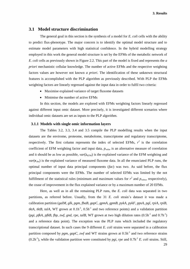
3. Results
29
3.1 Model structure discrimination
The general goal in this section is the synthesis of a model for E. coli cells with the ability
to predict flux-phenotype. The major concern is to identify the optimal model structure and to
estimate model parameters with high statistical confidence. In the hybrid modelling strategy
employed in this work the general model structure is set by the EFMs of the metabolic network of
E. coli cells as previously shown in Figure 2.2. This part of the model is fixed and represents the a
priori mechanistic cellular knowledge. The number of active EFMs and the respective weighting
factors values are however not known a priori. The identification of these unknown structural
features is accomplished with the PLP algorithm as previously described. With PLP the EFMs
weighting factors are linearly regressed against the input data in order to fulfil two criteria:
Maximise explained variance of target fluxome datasets
Minimise the number of active EFMs
In this section, the models are explored with EFMs weighting factors linearly regressed
against different input omic dataset. More precisely, it is investigated different scenarios where
individual omic datasets are set as inputs to the PLP algorithm.
3.1.1 Models with single omic information layers
The Tables 3.2, 3.3, 3.4 and 3.5 compile the PLP modelling results when the input
datasets are the envirome, proteome, metabolome, transcriptome and regulatory transcriptome,
respectively. The first column represents the index of selected EFMs, r2 is the correlation
coefficient of EFM weighting factor and input data, pvalue is an alternative measure of correlation
and it should be as low as possible, var(λEFM) is the explained variance of the EFM weighting and
var(robs) is the explained variance of measured fluxome data. In all the enunciated PLP runs, the
optimal number of input data principal components (fac) was two. As said before, the flux
principal components were the EFMs. The number of selected EFMs was limited by the not
fulfillment of the statistical rules (minimum and maximum values for r2 and pvaleu, respectively),
the cease of improvement in the flux explained variance or by a maximum number of 20 EFMs.
Here, as well as in all the remaining PLP runs, the E. coli data was separated in two
partitions, as referred before. Usually, from the 31 E. coli strain’s dataset it was made a
calibration partition (galM, glk, pgm, fbaB, gapC, gpmA, gpmB, pykA, pykF, ppsA, pgl, rpiA, rpiB,
tktA, tktB, talA, WT grown at 0.1h-1
, 0.5h-1
and two reference points) and a validation partition
(pgi, pfkA, pfkB, fbp, zwf, gnd, rpe, talB, WT grown at two high dilution rates (0.5h-1
and 0.7h-1
)
and a reference data point). The exception was the PLP runs which included the regulatory
transcriptional dataset. In such cases the 9 different E. coli strains were separated in a calibration
partition composed by pgm, gapC, zwf and WT strains grown at 0.5h-1
and two reference strains
(0.2h-1
), while the validation partition were constituted by pgi, rpe and 0.7h-1
E. coli strains. Still,
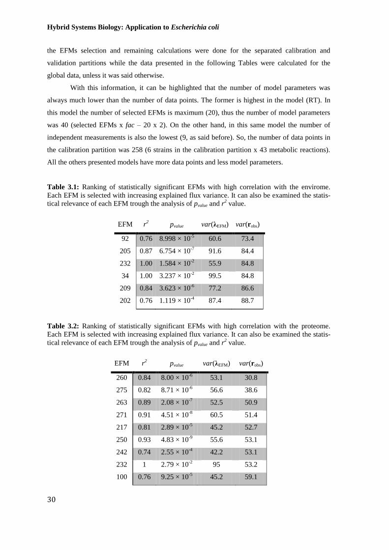
Hybrid Systems Biology: Application to Escherichia coli
30
the EFMs selection and remaining calculations were done for the separated calibration and
validation partitions while the data presented in the following Tables were calculated for the
global data, unless it was said otherwise.
With this information, it can be highlighted that the number of model parameters was
always much lower than the number of data points. The former is highest in the model (RT). In
this model the number of selected EFMs is maximum (20), thus the number of model parameters
was 40 (selected EFMs x fac – 20 x 2). On the other hand, in this same model the number of
independent measurements is also the lowest (9, as said before). So, the number of data points in
the calibration partition was 258 (6 strains in the calibration partition x 43 metabolic reactions).
All the others presented models have more data points and less model parameters.
Table 3.1: Ranking of statistically significant EFMs with high correlation with the envirome.
Each EFM is selected with increasing explained flux variance. It can also be examined the statis-
tical relevance of each EFM trough the analysis of pvalue and r2 value.
EFM r2 pvalue var(λEFM) var(robs)
92 0.76 8.998 × 10⁻⁵
60.6 73.4
205 0.87 6.754 × 10⁻⁷
91.6 84.4
232 1.00 1.584 × 10⁻²
55.9 84.8
34 1.00 3.237 × 10⁻²
99.5 84.8
209 0.84 3.623 × 10⁻⁶
77.2 86.6
202 0.76 1.119 × 10⁻⁴
87.4 88.7
Table 3.2: Ranking of statistically significant EFMs with high correlation with the proteome.
Each EFM is selected with increasing explained flux variance. It can also be examined the statis-
tical relevance of each EFM trough the analysis of pvalue and r2 value.
EFM r2 pvalue var(λEFM) var(robs)
260 0.84 8.00 × 10⁻⁶
53.1 30.8
275 0.82 8.71 × 10⁻⁶
56.6 38.6
263 0.89 2.08 × 10⁻⁷
52.5 50.9
271 0.91 4.51 × 10⁻⁸
60.5 51.4
217 0.81 2.89 × 10⁻⁵
45.2 52.7
250 0.93 4.83 × 10⁻⁹
55.6 53.1
242 0.74 2.55 × 10⁻⁴
42.2 53.1
232 1 2.79 × 10⁻²
95 53.2
100 0.76 9.25 × 10⁻⁵
45.2 59.1

3. Results
31
Table 3.2 (cont.): Ranking of statistically significant EFMs with high correlation with the prote-
ome. Each EFM is selected with increasing explained flux variance. It can also be examined the
statistical relevance of each EFM trough the analysis of pvalue and r2 value.
EFM r2 pvalue var(λEFM) var(robs)
244 0.82 1.41 × 10⁻⁵
30 59.3
220 0.77 1.13 × 10⁻⁴
37.2 60
229 0.68 1.35 × 10⁻³
39.7 60.4
92 0.78 4.23 × 10⁻⁵
34.2 69.3
124 0.87 1.14 × 10⁻⁶
32.8 69.3
220 0.77 1.13 × 10⁻⁴
37.2 60
229 0.68 1.35 × 10⁻³
39.7 60.4
92 0.78 4.23 × 10⁻⁵
34.2 69.3
124 0.87 1.14 × 10⁻⁶
32.8 69.3
249 0.64 3.46 × 10⁻³
22.4 69.4
34 1 3.56 × 10⁻²
99.5 69.4
236 0.87 1.70 × 10⁻⁶
31.3 69.5
105 1 1.37 × 10⁻⁴
50.9 69.9
99 1 1.15 × 10⁻²
26.4 69.9
Table 3.3: Ranking of statistically significant EFMs with high correlation with the metabolome.
Each EFM is selected with increasing explained flux variance. It can also be examined the statis-
tical relevance of each EFM trough the analysis of pvalue and r2 value.
EFM r2 pvalue var(λEFM) var(robs)
260 0.86 2.55 × 10⁻⁶
66.6 31
219 0.88 3.91 × 10⁻⁷
52.4 54.5
271 0.89 3.56 × 10⁻⁷
68.6 54.7
275 0.82 8.04 × 10⁻⁶
48.6 59
249 0.93 1.37 × 10⁻⁸
66.9 61.5
274 0.83 4.78 × 10⁻⁶
38.8 64.3
228 0.84 8.51 × 10⁻⁶
56.9 64.7
253 0.98 8.45 × 10⁻³
58 65.1
242 0.81 3.13 × 10⁻⁵
47.2 65.1
252 0.78 8.45 × 10⁻⁵
45.9 65.2
250 0.97 3.91 × 10⁻¹²
79.3 65.4
240 0.78 9.61 × 10⁻⁵
42.1 65.4
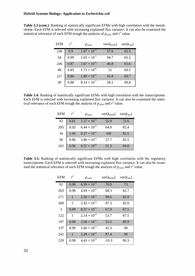
Hybrid Systems Biology: Application to Escherichia coli
32
Table 3.3 (cont.): Ranking of statistically significant EFMs with high correlation with the metab-
olome. Each EFM is selected with increasing explained flux variance. It can also be examined the
statistical relevance of each EFM trough the analysis of pvalue and r2 value.
EFM r2 pvalue var(λEFM) var(robs)
236 0.9 1.87 × 10⁻⁷
57.6 65.5
34 0.99 1.03 × 10⁻¹
94.7 65.5
246 0.87 1.67 × 10⁻⁶
46.8 65.6
48 0.85 1.73 × 10⁻⁶
51 69.5
227 0.86 1.89 × 10⁻⁶
41.8 69.7
30 0.88 8.14 × 10⁻⁷
28.1 69.8
Table 3.4: Ranking of statistically significant EFMs with high correlation with the transcriptome.
Each EFM is selected with increasing explained flux variance. It can also be examined the statis-
tical relevance of each EFM trough the analysis of pvalue and r2 value.
EFM r2 pvalue var(λEFM) var(robs)
92 0.81 1.37 × 10⁻⁵
55.9 72.6
205 0.92 6.44 × 10⁻⁹
64.9 82.4
34 1.00 8.27 × 10⁻⁴
100 82.5
30 0.80 3.80 × 10⁻⁵
57.7 82.5
202 0.90 6.57 × 10⁻⁸
51.3 84.8
Table 3.5: Ranking of statistically significant EFMs with high correlation with the regulatory
transcriptome. Each EFM is selected with increasing explained flux variance. It can also be exam-
ined the statistical relevance of each EFM trough the analysis of pvalue and r2 value.
EFM r2 pvalue var(λEFM) var(robs)
92 0.98 6.99 × 10⁻⁴
70.9 73
263 0.98 4.69 × 10⁻³
68.3 82.7
271 1 2.56 × 10⁻³
98.6 82.9
269 1 2.45 × 10⁻³
87.3 82.9
3 0.99 8.37 × 10⁻⁵
67.9 87.5
122 1 2.14 × 10⁻⁴
53.7 87.5
197 0.98 2.68 × 10⁻³
53.5 89.9
157 0.99 5.66 × 10⁻³
41.3 90
242 1 5.28 × 10⁻⁴
87.4 90
129 0.98 4.43 × 10⁻³
-10.3 90.3

3. Results
33
Table 3.5 (cont.): Ranking of statistically significant EFMs with high correlation with the regula-
tory transcriptome. Each EFM is selected with increasing explained flux variance. It can also be
examined the statistical relevance of each EFM trough the analysis of pvalue and r2 value.
EFM r2 pvalue var(λEFM) var(robs)
241 1 8.32 × 10⁻⁴
60.2 90.3
240 0.99 5.60 × 10⁻³
54.8 90.3
250 0.99 7.00 × 10⁻³
49.1 90.4
158 1 3.32 × 10⁻⁴
99.6 90.4
244 0.98 2.17 × 10⁻²
49.9 90.4
162 0.97 2.87 × 10⁻²
37 90.4
164 1 1.46 × 10⁻³
55.4 90.4
124 1 4.92 × 10⁻³
58.3 90.4
249 0.99 7.17 × 10⁻³
43.5 90.4
121 1 3.83 × 10⁻³
99.2 90.4
From these results it can be observed that the best performing model in terms of fluxome
prediction accuracy is the one that has as input data the regulatory transcriptome omic layer
(90.4% of explained variance of fluxome data) closely followed by the one that uses the envirome
layer (88.9% of explained variance of fluxome data). However, this transcriptional data is
available for fewer strains (9) than the remaining input datasets (31). This means that fewer
independent measurements are available. So, it precludes a fair comparison with the other
structures. Furthermore, when combined with other omic information, the validation partition
variance decreased (see Table 3.6 discussed below). For these two reasons (few data points and
possible overfitting) this structure was not selected for complete model identification in the next
sections. Later on, flux prediction from the regulatory transcriptome dataset will be discussed
(namely the reasons because it was not used for detailed examination and the possible
applications of a wider data collection) and also the results for the envirome dataset, second best
performing dataset in terms of explained variance and best mean squared error results, will be the
closely analysed.
3.1.2 Models with multiple omic information layers
Tables 3.6 and 3.7 show the model performance criteria for different combinations of
omic datasets as inputs for the metabolic fluxes calculation (the detailed EFMs selection results
for each case is shown in Appendix E). The data shown in the referred Appendix is similar to the
data showed earlier: the first column represents the index of selected EFMs, r2 is the correlation
coefficient of EFM weighting factor and input data, pvalue is another alternative measure of
Hybrid Systems Biology: Application to Escherichia coli
34
correlation and it should be as low as possible, var(λEFM) is the explained variance of the EFM
weightings and var(robs) is the explained variance of measured fluxome data. In all the next PLP
runs, the optimal number of input data principal components (fac) was also two. On the other
hand, the flux principal components were the EFMs. The number of selected EFMs was also
limited by the not fulfillment of the statistical rules (minimum and maximum values for r2 and
pvaleu, respectively), by the cease of the improvement of explained variance or by a maximum
number of 20 EFMs. Each line presents the fluxomes explained variance and the mean squared
error for the overall, calibration and validation datasets. As in the models described earlier, the
comparison between the number of model parameters and data points can also be done. The same
results can be seen here: the number of model parameters is much lower than the number of data
points.
Similarly, the E. coli data was separated in two partitions. Usually, from the 31 E. coli
strain’s dataset it was separated in a calibration partition composed by galM, glk, pgm, fbaB,
gapC, gpmA, gpmB, pykA, pykF, ppsA, pgl, rpiA, rpiB, tktA, tktB, talA, WT grown at 0.1h-1
, 0.5h-1
and two reference points) and a validation partition (pgi, pfkA, pfkB, fbp, zwf, gnd, rpe, talB, WT
grown at two high dilution rates (0.5h-1
and 0.7h-1
) and a reference data point). The exception was
the PLP runs which included the regulatory transcriptional dataset. In such cases the nine different
E. coli strains were separated in a calibration partition composed by pgm, gapC, zwf and WT
strains grown at 0.5h-1
and two reference strains (0.2h-1
), while the validation partition were
constituted by pgi, rpe and 0.7h-1
E. coli dataset.
These results show a coarse comparison between different model structures that integrate
different layers of omic information. It can be observed that the envirome alone is the most
informative omic layer in terms of flux prediction since this dataset obtained the lowest mean
squared error results for the validation partition, Table 3.6, and the second highest explained
variance for the validation partition, Table 3.7.
In the next sections, the best performing models are analysed in more detail. These
include the envirome model (E) and also the envirome and transcriptome combined model (E+T),
which ranked in second place in terms of mean squared error in the validation partition
(20722),Table 3.7, and explained variance of flux data in the validation dataset (85.2%),
Table 3.6.
It should be noted again that despite the apparent good results of the regulatory
transcriptome models (model RT), due to the lack of measurements and potential overfitting
problems when joint together with other omic datasets, this models will not be considered for
further detailed analysis.

3. Results
35
Table 3.6: Explained variance for all data points and for calibration and validation partition for
each PLP run with different omic factors. E: Envirome; P: Proteome; M: Metabolome; T: Tran-
scriptome; RT: Regulatory transcriptome; +: Different omic data was put together.
Omic factors Overall explained
variance (%)
Calibration partition
explained variance (%)
Validation partition ex-
plained variance (%)
E 88.7 88.83 88.52
P 69.9 76.71 64.40
M 69.8 84.32 58.14
T 84.8 90.04 80.55
RT 90.4 89.23 91.03
E+P 87.8 94.20 82.72
E+M 74.3 85.27 65.55
E+T 87.1 89.56 85.16
E+RT 89.7 91.07 64.26
P+M 71 78.92 64.55
P+T 89.1 93.12 85.85
P+TR 89.3 90.38 69.13
M+T 87.9 90.77 85.58
M+RT 92.1 93.03 74.83
T+RT 88.8 90.11 64.53
E+P+M 71.7 79.74 65.30
E+P+T 88.9 92.54 86.07
E+P+RT 89.1 90.15 70.63
E+M+T 86.7 89.50 84.45
E+M+RT 92.1 93.00 75.17
E+T+RT 88.8 90.18 64.09
P+M+T 87.2 90.13 84.83
P+M+RT 90.5 91.41 75.14
M+T+RT 92 92.89 76.27
E+P+M+T 86.2 89.56 83.58
E+P+M+RT 90.5 91.40 75.34
E+P+T+RT 88.8 90.20 64.53
E+M+T+RT 92 92.87 76.43
P+M+T+RT 90.2 91.13 73.83
E+P+M+T+RT 90.2 91.12 74.00
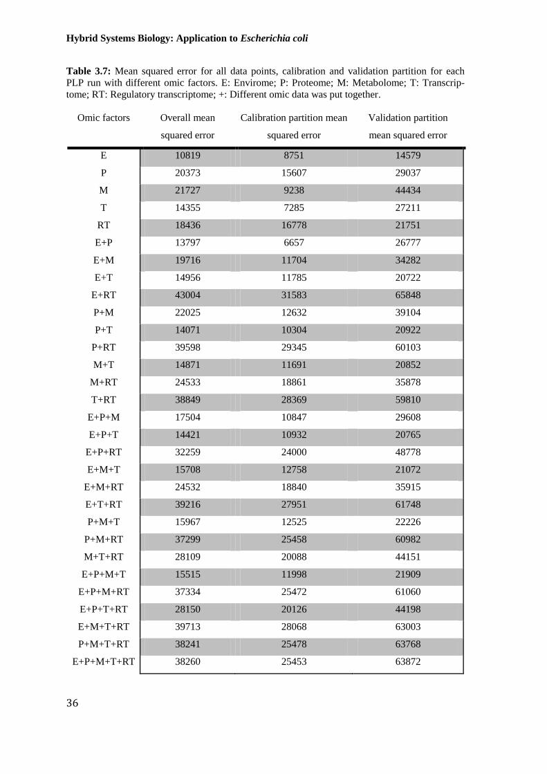
Hybrid Systems Biology: Application to Escherichia coli
36
Table 3.7: Mean squared error for all data points, calibration and validation partition for each
PLP run with different omic factors. E: Envirome; P: Proteome; M: Metabolome; T: Transcrip-
tome; RT: Regulatory transcriptome; +: Different omic data was put together.
Omic factors Overall mean
squared error
Calibration partition mean
squared error
Validation partition
mean squared error
E 10819 8751 14579
P 20373 15607 29037
M 21727 9238 44434
T 14355 7285 27211
RT 18436 16778 21751
E+P 13797 6657 26777
E+M 19716 11704 34282
E+T 14956 11785 20722
E+RT 43004 31583 65848
P+M 22025 12632 39104
P+T 14071 10304 20922
P+RT 39598 29345 60103
M+T 14871 11691 20852
M+RT 24533 18861 35878
T+RT 38849 28369 59810
E+P+M 17504 10847 29608
E+P+T 14421 10932 20765
E+P+RT 32259 24000 48778
E+M+T 15708 12758 21072
E+M+RT 24532 18840 35915
E+T+RT 39216 27951 61748
P+M+T 15967 12525 22226
P+M+RT 37299 25458 60982
M+T+RT 28109 20088 44151
E+P+M+T 15515 11998 21909
E+P+M+RT 37334 25472 61060
E+P+T+RT 28150 20126 44198
E+M+T+RT 39713 28068 63003
P+M+T+RT 38241 25478 63768
E+P+M+T+RT 38260 25453 63872
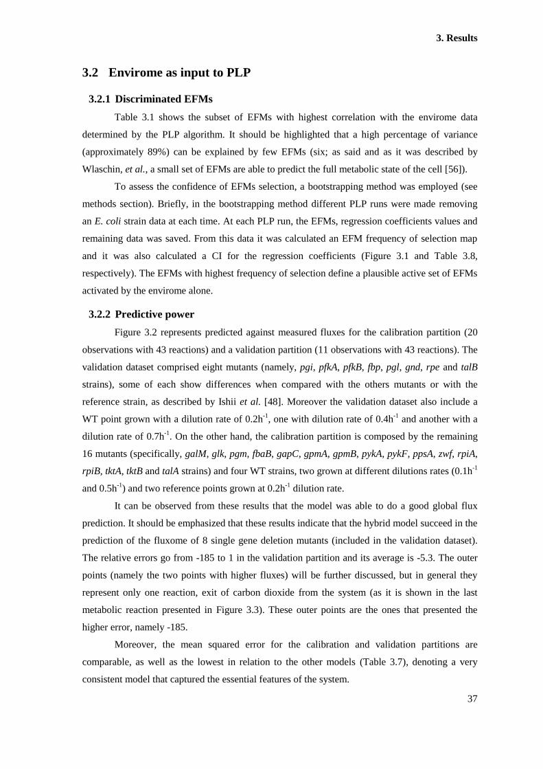
3. Results
37
3.2 Envirome as input to PLP
3.2.1 Discriminated EFMs
Table 3.1 shows the subset of EFMs with highest correlation with the envirome data
determined by the PLP algorithm. It should be highlighted that a high percentage of variance
(approximately 89%) can be explained by few EFMs (six; as said and as it was described by
Wlaschin, et al., a small set of EFMs are able to predict the full metabolic state of the cell [56]).
To assess the confidence of EFMs selection, a bootstrapping method was employed (see
methods section). Briefly, in the bootstrapping method different PLP runs were made removing
an E. coli strain data at each time. At each PLP run, the EFMs, regression coefficients values and
remaining data was saved. From this data it was calculated an EFM frequency of selection map
and it was also calculated a CI for the regression coefficients (Figure 3.1 and Table 3.8,
respectively). The EFMs with highest frequency of selection define a plausible active set of EFMs
activated by the envirome alone.
3.2.2 Predictive power
Figure 3.2 represents predicted against measured fluxes for the calibration partition (20
observations with 43 reactions) and a validation partition (11 observations with 43 reactions). The
validation dataset comprised eight mutants (namely, pgi, pfkA, pfkB, fbp, pgl, gnd, rpe and talB
strains), some of each show differences when compared with the others mutants or with the
reference strain, as described by Ishii et al. [48]. Moreover the validation dataset also include a
WT point grown with a dilution rate of 0.2h-1
, one with dilution rate of 0.4h-1
and another with a
dilution rate of 0.7h-1
. On the other hand, the calibration partition is composed by the remaining
16 mutants (specifically, galM, glk, pgm, fbaB, gapC, gpmA, gpmB, pykA, pykF, ppsA, zwf, rpiA,
rpiB, tktA, tktB and talA strains) and four WT strains, two grown at different dilutions rates (0.1h-1
and 0.5h-1
) and two reference points grown at 0.2h-1
dilution rate.
It can be observed from these results that the model was able to do a good global flux
prediction. It should be emphasized that these results indicate that the hybrid model succeed in the
prediction of the fluxome of 8 single gene deletion mutants (included in the validation dataset).
The relative errors go from -185 to 1 in the validation partition and its average is -5.3. The outer
points (namely the two points with higher fluxes) will be further discussed, but in general they
represent only one reaction, exit of carbon dioxide from the system (as it is shown in the last
metabolic reaction presented in Figure 3.3). These outer points are the ones that presented the
higher error, namely -185.
Moreover, the mean squared error for the calibration and validation partitions are
comparable, as well as the lowest in relation to the other models (Table 3.7), denoting a very
consistent model that captured the essential features of the system.

Hybrid Systems Biology: Application to Escherichia coli
38
Figure 3.1: Frequency of selection of each EFM in the bootstrapping validation procedure when
envirome is the input data.
Figure 3.2: Predicted against measured fluxes with envirome as input to PLP for the calibration
partition (blue circles) and validation partition (grey triangles).
As illustrative examples Figure 3.3A and Figure 3.3B show the prediction of a reference
WT and mutant talB, respectively (both included in the validation dataset). The behaviour of both
strains is quite different (as described by Ishii et al. [48]). Such biological alterations in the
mutant strain when compared with the WT are especially noticeable in the protein concentration,
gene expression, metabolite concentration and metabolic reaction rate that were directly related
with such modification, this will be detailed examined in the Discussion section.
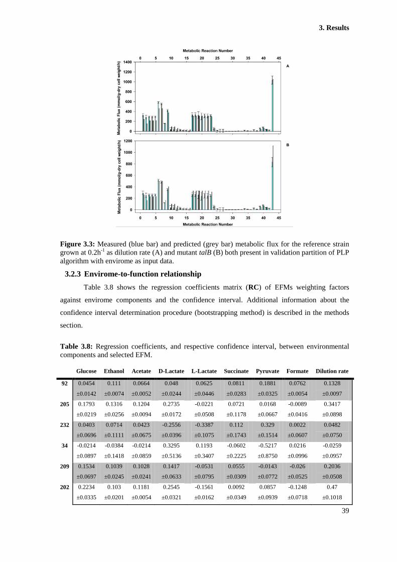
3. Results
39
Figure 3.3: Measured (blue bar) and predicted (grey bar) metabolic flux for the reference strain
grown at 0.2h-1
as dilution rate (A) and mutant talB (B) both present in validation partition of PLP
algorithm with envirome as input data.
3.2.3 Envirome-to-function relationship
Table 3.8 shows the regression coefficients matrix (RC) of EFMs weighting factors
against envirome components and the confidence interval. Additional information about the
confidence interval determination procedure (bootstrapping method) is described in the methods
section.
Table 3.8: Regression coefficients, and respective confidence interval, between environmental
components and selected EFM.
Glucose Ethanol Acetate D-Lactate L-Lactate Succinate Pyruvate Formate Dilution rate
92 0.0454
±0.0142
0.111
±0.0074
0.0664
±0.0052
0.048
±0.0244
0.0625
±0.0446
0.0811
±0.0283
0.1881
±0.0325
0.0762
±0.0054
0.1328
±0.0097
205 0.1793
±0.0219
0.1316
±0.0256
0.1204
±0.0094
0.2735
±0.0172
-0.0221
±0.0508
0.0721
±0.1178
0.0168
±0.0667
-0.0089
±0.0416
0.3417
±0.0898
232 0.0403
±0.0696
0.0714
±0.1111
0.0423
±0.0675
-0.2556
±0.0396
-0.3387
±0.1075
0.112
±0.1743
0.329
±0.1514
0.0022
±0.0607
0.0482
±0.0750
34 -0.0214
±0.0897
-0.0384
±0.1418
-0.0214
±0.0859
0.3295
±0.5136
0.1193
±0.3407
-0.0602
±0.2225
-0.5217
±0.8750
0.0216
±0.0996
-0.0259
±0.0957
209 0.1534
±0.0697
0.1039
±0.0245
0.1028
±0.0241
0.1417
±0.0633
-0.0531
±0.0795
0.0555
±0.0309
-0.0143
±0.0772
-0.026
±0.0525
0.2036
±0.0508
202 0.2234
±0.0335
0.103
±0.0201
0.1181
±0.0054
0.2545
±0.0321
-0.1561
±0.0162
0.0092
±0.0349
0.0857
±0.0939
-0.1248
±0.0718
0.47
±0.1018
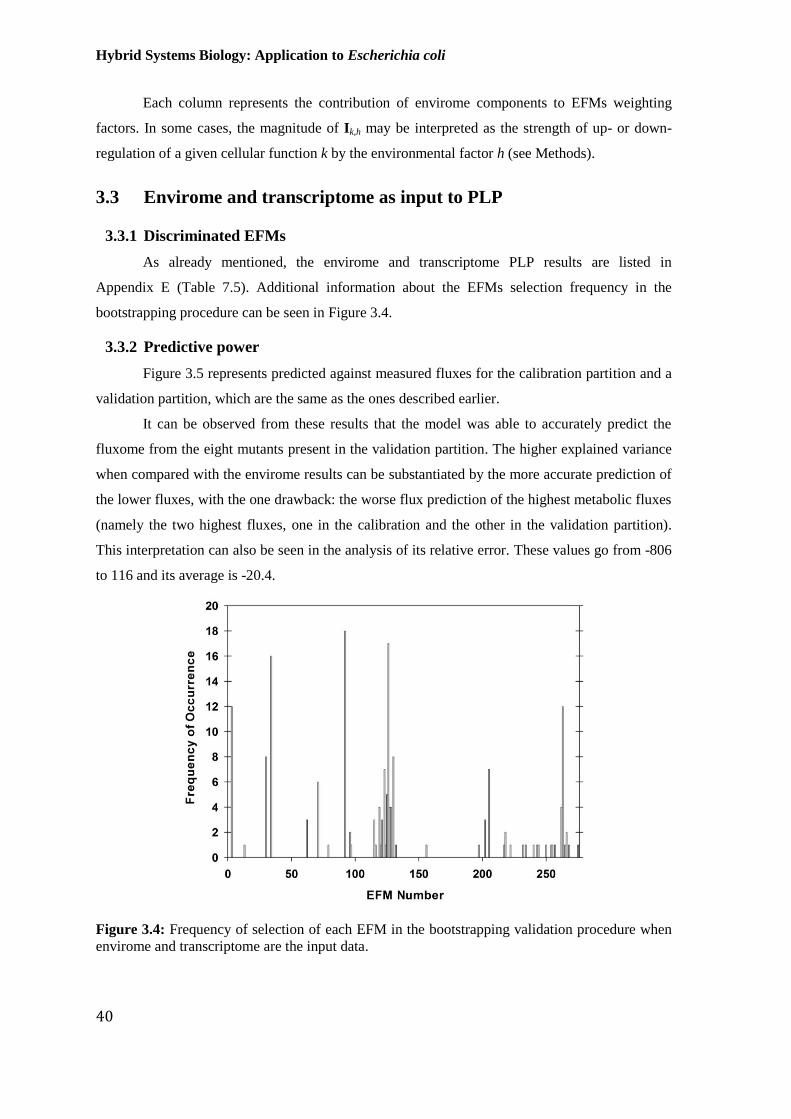
Hybrid Systems Biology: Application to Escherichia coli
40
Each column represents the contribution of envirome components to EFMs weighting
factors. In some cases, the magnitude of Ik,h may be interpreted as the strength of up- or down-
regulation of a given cellular function k by the environmental factor h (see Methods).
3.3 Envirome and transcriptome as input to PLP
3.3.1 Discriminated EFMs
As already mentioned, the envirome and transcriptome PLP results are listed in
Appendix E (Table 7.5). Additional information about the EFMs selection frequency in the
bootstrapping procedure can be seen in Figure 3.4.
3.3.2 Predictive power
Figure 3.5 represents predicted against measured fluxes for the calibration partition and a
validation partition, which are the same as the ones described earlier.
It can be observed from these results that the model was able to accurately predict the
fluxome from the eight mutants present in the validation partition. The higher explained variance
when compared with the envirome results can be substantiated by the more accurate prediction of
the lower fluxes, with the one drawback: the worse flux prediction of the highest metabolic fluxes
(namely the two highest fluxes, one in the calibration and the other in the validation partition).
This interpretation can also be seen in the analysis of its relative error. These values go from -806
to 116 and its average is -20.4.
Figure 3.4: Frequency of selection of each EFM in the bootstrapping validation procedure when
envirome and transcriptome are the input data.

3. Results
41
Figure 3.5: Predicted against measured fluxes with proteome and transcriptome as input to PLP
for the calibration partition (blue circles) and validation partition (grey triangles).
Figure 3.6A and Figure 3.6B represent the same illustrative examples shown before
(reference WT and mutant talB, respectively; both included in the validation dataset). In these
examples, the over prediction of the last metabolic reaction on Figure 3.6B is more evident, this
may be due to the number of selected EFMs as will be proposed.
3.3.3 Relationship between input and cellular function
Figure 3.7 shows the regression coefficients of EFMs (cellular functions) weighting
factors against envirome and transcriptome components (input data). This information is not
shown in the form of a table due to its overwhelming size. Here the only CI values presented will
be the ones attached to the EFMs up- or down-regulation effects discussed in the next section.
The remaining CI values will not be presented due to its size.
A global analysis over the Figure 3.7 shows that the main up-regulation effects on the
EFMs 92, 126 and 127 undergoes by the last environmental factor (high concentrations of
succinate and pyruvate in the culture medium) and by the sixty-ninth transcriptional factors,
fumC, in the EFM 127.
On the other hand, the negative influences are more distributed over all the metabolic
functions. However, they are more present in the last selected EFMs (125 and 127). Such down-
regulation is clear in the tenth to twentieth omic index factor zone.
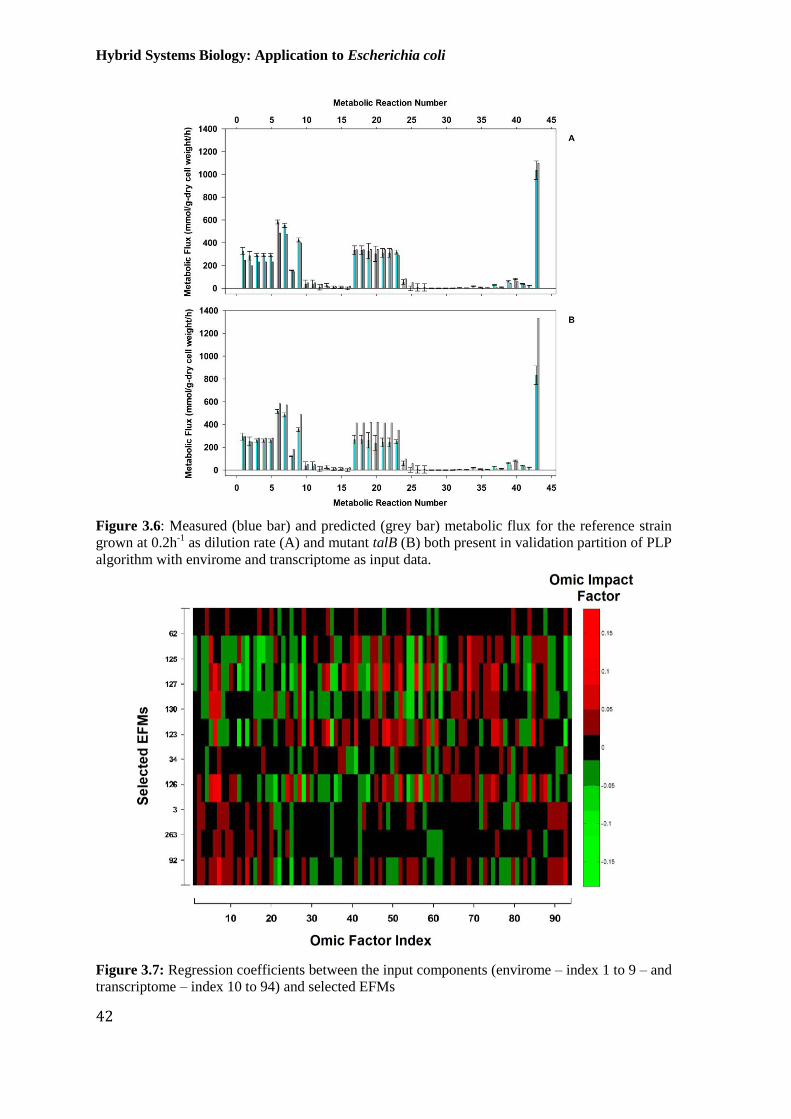
Hybrid Systems Biology: Application to Escherichia coli
42
Figure 3.6: Measured (blue bar) and predicted (grey bar) metabolic flux for the reference strain
grown at 0.2h-1
as dilution rate (A) and mutant talB (B) both present in validation partition of PLP
algorithm with envirome and transcriptome as input data.
Figure 3.7: Regression coefficients between the input components (envirome – index 1 to 9 – and
transcriptome – index 10 to 94) and selected EFMs

4 Discussion

Hybrid Systems Biology: Application to Escherichia coli
44
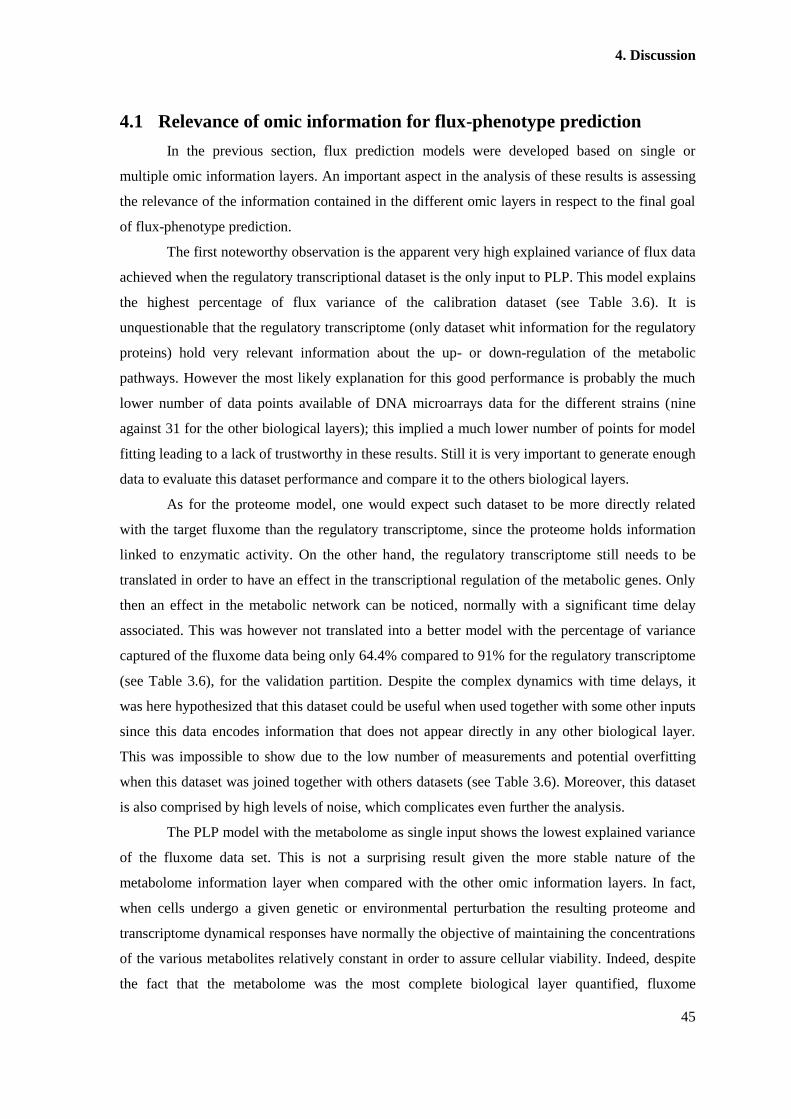
4. Discussion
45
4.1 Relevance of omic information for flux-phenotype prediction
In the previous section, flux prediction models were developed based on single or
multiple omic information layers. An important aspect in the analysis of these results is assessing
the relevance of the information contained in the different omic layers in respect to the final goal
of flux-phenotype prediction.
The first noteworthy observation is the apparent very high explained variance of flux data
achieved when the regulatory transcriptional dataset is the only input to PLP. This model explains
the highest percentage of flux variance of the calibration dataset (see Table 3.6). It is
unquestionable that the regulatory transcriptome (only dataset whit information for the regulatory
proteins) hold very relevant information about the up- or down-regulation of the metabolic
pathways. However the most likely explanation for this good performance is probably the much
lower number of data points available of DNA microarrays data for the different strains (nine
against 31 for the other biological layers); this implied a much lower number of points for model
fitting leading to a lack of trustworthy in these results. Still it is very important to generate enough
data to evaluate this dataset performance and compare it to the others biological layers.
As for the proteome model, one would expect such dataset to be more directly related
with the target fluxome than the regulatory transcriptome, since the proteome holds information
linked to enzymatic activity. On the other hand, the regulatory transcriptome still needs to be
translated in order to have an effect in the transcriptional regulation of the metabolic genes. Only
then an effect in the metabolic network can be noticed, normally with a significant time delay
associated. This was however not translated into a better model with the percentage of variance
captured of the fluxome data being only 64.4% compared to 91% for the regulatory transcriptome
(see Table 3.6), for the validation partition. Despite the complex dynamics with time delays, it
was here hypothesized that this dataset could be useful when used together with some other inputs
since this data encodes information that does not appear directly in any other biological layer.
This was impossible to show due to the low number of measurements and potential overfitting
when this dataset was joined together with others datasets (see Table 3.6). Moreover, this dataset
is also comprised by high levels of noise, which complicates even further the analysis.
The PLP model with the metabolome as single input shows the lowest explained variance
of the fluxome data set. This is not a surprising result given the more stable nature of the
metabolome information layer when compared with the other omic information layers. In fact,
when cells undergo a given genetic or environmental perturbation the resulting proteome and
transcriptome dynamical responses have normally the objective of maintaining the concentrations
of the various metabolites relatively constant in order to assure cellular viability. Indeed, despite
the fact that the metabolome was the most complete biological layer quantified, fluxome
Hybrid Systems Biology: Application to Escherichia coli
46
explained variance was substantially lower than others much more incomplete layers of
information such as the proteome (model P) or the envirome (model E).
The PLP model that uses the envirome dataset as input (model E) is the second best
performing model in terms of explained variance of fluxome data and also the one with lowest
mean squared error of prediction (see Table 3.6 and Table 3.7, respectively). This result is
concordant with the research of Kell et al. and Allen et al.. These studies have shown that the
number of metabolites excreted or secreted to the environment is very high and that the variations
of the envirome are much higher than the metabolome and also more easily and accurately
measured [57]. These authors have clearly demonstrated through statistical analysis that
exometabolome data enables to discriminate single gene deletion mutants of yeast cells [58].
Although the characterization of the envirome in this work was the most incomplete in relation to
the other omic layers, the results obtained in the present thesis clearly support the discrimination
of single gene deletion mutants using the envirome only. But even further than that, it is shown
here that the envirome analysis enables not only the discrimination but also an accurate prediction
of flux phenotype of the KO mutants.
It could be argued that the regulatory transcriptome responds to the external impulses and,
although it may have a time lapse, it comprises more or complementary information to the partial
environmental data used in this work (only organic compounds). Contrary to this hypothesis, the
results obtained with the E+T model, although quite good (the second best), they do not show a
significant improvement in relation to the envirome model.
4.2 Envirome flux prediction analysis
In this section, it will be discussed the results obtained with the envirome as input to PLP
model.
4.2.1 Discriminated EFMs
The first EFM selected by PLP is EFM 92, with 85% of frequency of selection (calculated
by the bootstrapping method – Figure 3.1). EFM 92 is partially constituted by glycolysis and
tricarboxylic acid cycle, and it belongs to the small group of EFMs that exclusively produces
energy. Moreover, within the analysed KO mutants group present in both calibration and
validation partitions (see section 2.6.3 on page 23), EFM 92 is a plausible EFM in all KO mutants
except in the strain in which pgi gene is deleted, which adds consistency to this result.
Others frequently selected EFMs are EFMs 209 and 232 (see Table 3.1). These EFMs
together with EFM 92 comprise all the metabolic reactions involved in the three considered
pathways (glycolysis, tricarboxylic acid cycle and pentose phosphate pathway) in such a
combination that at least one of them is in theory plausible in every E. coli strain considered. As
said before the EFM 92 is the only pathway that functions exclusively for energy production. All

4. Discussion
47
the remaining EFMs besides energy also produce additional building blocks that could be used in
biosynthesis (acetate in the case of EFM 209 and fructose-6-phosphate and erythrose-4-phosphate
in the case of EFM 232). Depending on the global EFMs reaction products, the EFMs functions
can be inferred through the analysis of the fate of such end-products in the cell. For instance,
fructose-6-phosphate can be used in the production of others hydrocarbons or in the production of
the cellular wall, namely through the production of peptidoglycan. On the other hand, the
erythrose-4-phosphate utilization can be traced to the production of several amino acids like
tryptophan, phenylalanine and tyrosine. All the remaining EFMs functions listed in Table 3.1 can
be consulted in the supplementary material trough the participating reactions and its global
products (as described by Schwartz, et al. [59]).
The second layer of frequently selected EFMs is formed by EFMs 3, 202, 205 and 263.
However they are usually selected in two sets (EFM 3+263 and EFM 202+205). The two sets
confer the same functionality, namely the production of oxaloacetate, pyruvate and acetyl
coenzyme-A required for biosynthesis. These are vital precursors for the cell to grow, whose
fluxes carry a significant variance that needs to be explained. What seems to happen is that for
some KO mutants EFM 3+263 are unfeasible while for other it is the group EFM 202+205 that is
unfeasible. This justifies the mutually excluding selection observed in the PLP results.
The EFM selected with lowest frequency is EFM 34. This may be related to the fact that
the metabolic function of this EFM is redundant with the function of EFM 232, i.e., both EFMs
produce erythrose 4-phosphate. Moreover, this EFM is only feasible in pgl, ripA and tktA E. coli
strains, so this may also be one fact for the EFM selection since this cases may have unexplained
fluxes that have been fully explained in the remaining cases.
4.2.2 Predictive power
As shown in Figure 3.2, the envirome model succeeds in the prediction of the fluxome of
several gene deletion mutants with high accuracy. This result is to some extent surprising in light
of the potential perturbations that the deletion of a gene can have in the physiology of a cell,
which includes perturbations in the metabolome, proteome and transcriptome.
As said before, usually, after the internal (genetic) perturbation, not many metabolic
reactions are in theory directly affected. When compared to the full size metabolic network, such
perturbations are very localized to the metabolic reactions tightly related to the deleted one. This
localized nature of genetic perturbations could be confirmed through the analysis of the
metabolome, proteome and transcriptome.
One example is the talB single gene deletion mutant (Figure 3.3B). In this strain the
concentration of sedoheptulose 7-phosphate, a reactant that participates in the metabolic reaction
catalysed by the removed protein (reaction 16 in the metabolic network) drastically increased.
Moreover, the concentration of some others metabolites not directly related to this protein also

Hybrid Systems Biology: Application to Escherichia coli
48
changed (like the concentration of glucose-6-phosphate, ribose-5-phosphate and
ribulose-5-phosphate). The effects of these perturbations can also be traced in the proteome (since
AcnB expression index reduced to half and SdhB expression index doubled, both proteins
participate in the tricarboxylic acid cycle).
Nevertheless, despite the visible but localized perturbations in the biological system, as
whole one can conclude that the deletion of a single gene does not have a dramatic effect on the
metabolism. An important indication of this is that all the analysed mutants are viable.
Particularly, it seems that the deletion of a single gene does not perturb significantly the
relationship between the cellular metabolism and the envirome, which is likely to be conserved
within the same species. This could explain the success of the envirome model in predicting
several single gene deletion mutants.
Among the 43 metabolic reactions, the last reaction in the network is systematically over
predicted with a higher error associated. This can be observed in the Figure 3.2 as the two highest
fluxes correspond to the referred metabolic reaction in the E. coli strain grown at 0.5h-1
and 0.7h-1
.
Reaction 43 is peculiar in that it codes for the exit of CO2 from the system and is involved in all
the EFMs. This modelling discrepancy is mostly associated to the difficulty in closing the carbon
balance in the identified reduced metabolic models with a small number of EFMs.
4.2.3 Envirome function mapping
In this section, the identified relation patterns between envirome components and
metabolic functions are analysed on the basis of the regression coefficients matrix delivered by
the PLP algorithm (see Table 3.8 and Figure 2.3).
As first note, it should be commented that the computation of confidence intervals of
regression coefficients by the bootstrapping method clearly shoes that many of the values
obtained are not statistically consistent, precluding taking rigorous conclusions about the effect of
several envirome components on several metabolic functions. This is the case of, for instance,
EFM 34. This EFM is only feasible in pgl, ripA and tktA E. coli strains. So, since there are few
data points that can be used to calculate these regression coefficients, their confidence intervals
are very large. Moreover, EFM 34 has a similar function to the EFM 232, which is also
theoretically feasible in the referred strains. Framed by these practical constraints, the discussion
that follows will be centred in those results that are statistical consistent.
So, one of the first things that stands out is the generally strong positive correlation
between the weighting factors of almost all the EFMs and the glucose concentration and also the
reaction dilution rate (see Table 3.8). These results are very consistent with the fact that glucose is
the single carbon source and also that all the EFMs have either an energy production function or a
biosynthetic function. As such, the higher the glucose concentration or the dilution rate value, the
higher are the fluxes through the active pathways. Since glucose is the only carbon source in this
4. Discussion
49
system, a positive regulation coefficient should be the most likely outcome.
In the same way, the acetate, ethanol and (D- and L-) lactate regression coefficients show
mostly a positive correlation with the pathways presented in the Table 3.8. This may suggest that
when the fluxes upstream to the tricarboxylic acid cycle are very high they might be deflected to
the production of these by-products. In this case, the positive correlation does not correspond to a
regulatory effect triggered by environmental factors. Rather it represents an environmental change
caused by an overflow in the metabolic pathways, which resulted in the accumulation of
metabolic by-products in the extracellular medium. This condition is especially obvious in the
case of EFM 202. The main product of EFM 202 is acetate, thus not surprisingly, EFM 202
weighting factor shows positive correlation with acetate concentration in the medium.
In another example, formate can be produced as an incomplete oxidized by-product of the
formation of acetyl coenzyme-A from pyruvate (not included in the metabolic network). As
expected the accumulation of formate in the medium correlates positively with EFM 92, which
includes a reaction composed by the formation of acetyl coenzyme-A from pyruvate, and
negatively with EFM 202, which does not include the referred reaction. Both regression
coefficients have low CI suggesting a high confidence in this result.
Until now the discussion was focused on global interaction patterns between the envirome
and fluxome. However, this relationship is the result of several molecular level interaction
mechanisms that goes across the multiple omic layers. The envirome components can interact
with genes through sensing and regulatory proteins, which will activate or repress their
expression [60]. Environmental factors can also exhibit, for instance, some allosteric interactions
with enzymes (metabolites) or have other regulatory effects caused by abiotic factors such as
temperature [61]. In many cases, a given environmental perturbation is followed by changes
(either they are in a set of proteins activities or the transcriptional expression of some genes),
which eventually will influence the fluxome.
So, looking closely at the regulation properties, for instance in the case of pyruvate, the
effect can be traced through the regulatory protein IclR, in which pyruvate works as ligand. It has
been reported [62] that when pyruvate is present in high concentration, a AceB-IclR-pyruvate
complex is formed as a safety mechanism to quickly repress the glyoxylate shunt. In Table 3.8
can be seen that pyruvate correlates negatively with the EFM 34 that involves the glyoxylate
shunt (reactions 26 and 27).
Furthermore, the reflex of this effect can be seen in the ripA and tktA mutant. In these
cases the extracellular and intracellular pyruvate concentration is one of the highest among all
mutants. This had the consequence of decreasing the protein expression from the operon aceBAK
(also the concentration of these proteins are one of the lowest in the referred cases when
compared with the others mutant strains). This might be also a reason for the negative regression

Hybrid Systems Biology: Application to Escherichia coli
50
coefficients between pyruvate and EFM34.
Other metabolic effects can also be seen in the relationship between the PykF expression
index and the extracellular pyruvate concentration, which show a positive correlation, that is,
when the protein expression increases, pyruvate concentration also increases. The protein
expression increase may occur due to the increase of fructose-1-phosphate intracellular
concentration, which is the only metabolite with reported regulation properties of this gene
expression (if the metabolite is present, the FruR transcriptional regulator becomes inactive and
does not block the pykF transcriptional initiation [62]). A plausible explanation for the
fructose-1-phosphate concentration increase is the increase of others closely related metabolites
like fructose-6-phosphate and fructose-1,6-phosphate, involved in glycolysis. So, if these
metabolites increase the remaining glycolysis metabolite can also increase, namely the pyruvate
intracellular concentration (last metabolite in glycolysis) and so, when pyruvate intracellular
concentration is high the respective extracellular concentration also increases. Again, this may be
one of the regulation mechanism reflected in the regression coefficient of pyruvate in EFM 92,
which involves the reaction 8 (production of pyruvate from phosphoenolpyruvate, catalysed by
PykF).
Similar mechanisms can be found with regulatory protein LldR which senses L-lactate.
However, it has little influence in the protein concentration because it is maintained constant in
the majority of the referred cases. This may be explained by others regulatory mechanisms that
influences this metabolic function, like for instance translation regulation or its turnover process.
4.3 Envirome and transcriptome flux prediction analysis
Here discussion is focused on the differences between the envirome (E) and the envirome
and transcriptome (E+T) models rather than exhaustive regulation interpretation.
4.3.1 Discriminated EFMs
When comparing Table 7.5 with Table 3.1, it is clear that the global prediction power of
both methods is comparable (87.1% and 88.7%, respectively). The same occurs in the explained
flux variance in the validation partition (88.5% and 85.1%, respectively). It is unquestionable that
the transcriptome dataset may have important information for the flux prediction, yet it can also
have some redundant information or some transcriptional evidence that is not relevant for these
metabolic functions. This may complicate model development eventually resulting in a
degradation of overall flux prediction results (as has been described, the mRNA concentration
does not have a direct relationship between the protein concentration nor with its metabolic rate
rather it depends on many other interactions besides the described one [63]).
However, when it is added this dataset to the environmental information, there are some
modification in the selected metabolic function. For instance, in this PLP run there were selected
4. Discussion
51
the 2-keto-glutarate, phosphoenolpyruvate, 3-phosphoglycerate, glyceraldehyde 3-phosphate and
ethanol production, which was not been selected when the envirome dataset were given to PLP as
only input. This means that the metabolic function of, for instance, production of some amino
acids like tyrosine (through the utilization of 2-keto-glutarate), or serine (using 3-
phosphoglycerate) are in some way related with the transcriptional level of the analysed genes.
However, if there were to be determined exhaustively all the environmental factors concentration
probably the flux prediction could be even better or it could select more metabolic function.
4.3.2 Input data to function relationship
Just as illustrative example, some of the omic factors that always show positive
correlation with the selected EFMs are succinate and acs, column six and 64 from Figure 3.7. In
the former case, it may be related with the utilization of succinate in almost all the selected EFMs
(except in the last one, which has the lowest regression coefficient, 0.0053 and with relatively
high confidence interval, 0.072). On the other hand, the other example given is the acs gene,
which codes for the acetyl-CoA synthetase. Although the formation of acetyl-CoA is included in
the metabolic network, this enzyme is not directly involved since the catalysed reaction involves
the consumption of, for instance, acetate (which corresponds to the inverse reaction 29 in
Figure 2.1). Nevertheless, this relationship also makes sense, since all the EFMs selected have the
production of acetyl-CoA. So, although the mRNA production does not have a direct relationship
with the protein level nor with its enzymatic rates, this regulation property was expected due to
the close relationship between the acetyl-CoA production and the EFMs activation status.
On the other end are the other omic factors that have a consistently negative influence in
all the selected EFMs like fbp and lldd mRNA expression (16 and 78 columns in Figure 2.1,
respectively). These two genes code for two enzymes (fructose-1,6-bisphosphatase I and L-lactate
dehydrogenase) that catalyse two reactions that are not represented in the metabolic network. Yet
they represent the inverse reaction of reaction 3 and 30, respectively. In this way it is obvious that
they should have a negative influence in the EFMs that involve those reactions.

Hybrid Systems Biology: Application to Escherichia coli
52

5 Conclusions

Hybrid Systems Biology: Application to Escherichia coli
54

5. Conclusion
55
In this thesis, mathematical modelling tools were employed for the interpretation of
different layers of omic information of E. coli cells, collected from 24 single gene deletion mutant
experiments and WT strain experiments grown in 5 different conditions. In particular, a hybrid
computational algorithm was employed to identify correlation patterns between input omic data
sets (envirome, metabolome, proteome, transcriptome and regulatory transcriptome) with target
fluxome data sets. In the adopted algorithm, the target fluxome data was deconvoluted into
weighting factors of metabolic functions, which were linearly regressed against many input
variables. This enabled to map in a robust way redundant input data sets into sets of active
metabolic functions. Several combinations of input information were assessed in terms of
achieved prediction power of the target fluxome data.
One of the main conclusions to be taken from this study is that the envirome layer of
information is very important for metabolic function inference and ultimately metabolic flux
prediction. It should be highlighted in particular the ability of the PLP algorithm to predict the
fluxome of genetically modified strains or WT strains grown at different conditions on the basis
of envirome data and genome information alone.
The analysis of the PLP regression coefficients showed that the regression coefficients
could be used to infer envirome regulation mechanisms. Several of the identified regulation
mechanisms could be confirmed by the analysis of the remaining datasets. Such regulatory
mechanisms were previously described in other papers. However, it should be underlined that
these regulation factors are computed at a pathway level, so the most straightforward
interpretation scenario is that such regulatory coefficients are related to the rate-limiting step
within each EFM.
As corollary of the results above, one can conclude that the relationship between
envirome and metabolic function is to some extent conserved among genotype variants lacking
different genes. The deletion of a particular metabolic gene has the effect of deleting one or
several metabolic functions within the cells. Interestingly, this does not perturb the remaining
viable functions. As future study, it should be considered the full envirome data acquisition for a
genome wide fluxome prediction. It should also be studied if the environmental factors regulation
patterns are conserved not only among genotype variants of the same species but also among
different species, in different phylogenetic classes or even in different genus.
It is well known that the optimization of environmental factors, such as medium
composition or reactor nutrients feeding, play an important role in industrial biotechnological
process performance. Historically, these two factors (medium composition and genetic
modifications) have contributed to the increase of bioprocess performance. In a way, the results
produced in this thesis confirm the importance of the envirome information layer to infer and
predict metabolic functions. Furthermore, an important lesson to be learned is that the envirome

Hybrid Systems Biology: Application to Escherichia coli
56
layer can be used for effective metabolic function engineering. It can be used to systematically
discover regulatory patterns over metabolic functions, paving the way for a function oriented
environment engineering approach.
Finally, besides the many developed and applied modelling methods, the PLP algorithm
might have an important role in the future to unravel the regulatory patterns in redundant
biological systems that have not yet been mechanistically described in the literature. This can be
performed not only at an environmental level, but also at the level of metabolites and proteins,
particularly for elucidation of the role of transcription factors. With this knowledge, standard
biological parts can be better designed as building block for pathway level synthetic biology
developments.

6 References

Hybrid Systems Biology: Application to Escherichia coli
58

6. References
59
1. Barnes J: The complete works of Aristotle: the revised Oxford translation: Princeton
University Press; 1984.
2. Konopka AK: Systems biology: principles, methods, and concepts: CRC Press/Taylor
& Francis; 2007.
3. Fu P: Introduction. In: Systems Biology and Synthetic Biology. John Wiley & Sons, Inc.;
2009: 1-7.
4. Keseler IM, Collado-Vides J, Santos-Zavaleta A, Peralta-Gil M, Gama-Castro S, Muniz-
Rascado L, Bonavides-Martinez C, Paley S, Krummenacker M, Altman T et al: EcoCyc:
a comprehensive database of Escherichia coli biology. Nucleic Acids Res 2011,
39:D583-D590.
5. Gama-Castro S, Salgado H, Peralta-Gil M, Santos-Zavaleta A, Muñiz-Rascado L, Solano-
Lira H, Jimenez-Jacinto V, Weiss V, García-Sotelo JS, López-Fuentes A et al:
RegulonDB version 7.0: transcriptional regulation of Escherichia coli K-12
integrated within genetic sensory response units (Gensor Units). Nucleic Acids Res
2011, 39(suppl 1):D98-D105.
6. Reed JL, Palsson BO: Thirteen Years of Building Constraint-Based In Silico Models
of Escherichia coli. J Bacteriol 2003, 185(9):2692-2699.
7. Price ND, Reed JL, Palsson BO: Genome-scale models of microbial cells: evaluating
the consequences of constraints. Nat Rev Micro 2004, 2(11):886-897.
8. Mo ML, Jamshidi N, Palsson BO: A genome-scale, constraint-based approach to
systems biology of human metabolism. Mol Biosyst 2007, 3(9):598-603.
9. Famili I, Förster J, Nielsen J, Palsson BO: Saccharomyces cerevisiae phenotypes can
be predicted by using constraint-based analysis of a genome-scale reconstructed
metabolic network. Proceedings of the National Academy of Sciences 2003,
100(23):13134-13139.
10. Lee SY, Lee DY, Kim TY: Systems biotechnology for strain improvement. Trends
Biotechnol 2005, 23(7):349-358.
11. Orth JD, Thiele I, Palsson BO: What is flux balance analysis? Nat Biotechnol 2010,
28(3):245-248.
12. Covert MW, Knight EM, Reed JL, Herrgard MJ, Palsson BO: Integrating high-
throughput and computational data elucidates bacterial networks. Nature 2004,
429(6987):92-96.
13. Covert MW, Schilling CH, Palsson B: Regulation of Gene Expression in Flux Balance
Models of Metabolism. J Theor Biol 2001, 213(1):73-88.
14. Akesson M, Forster J, Nielsen J: Integration of gene expression data into genome-
scale metabolic models. Metab Eng 2004, 6(4):285-293.
15. Segrè D, Vitkup D, Church GM: Analysis of optimality in natural and perturbed
metabolic networks. Proceedings of the National Academy of Sciences 2002,
99(23):15112-15117.
16. Shlomi T, Berkman O, Ruppin E: Regulatory on/off minimization of metabolic flux
changes after genetic perturbations. Proc Natl Acad Sci U S A 2005, 102(21):7695-
7700.
17. Benyamini T, Folger O, Ruppin E, Shlomi T: Flux balance analysis accounting for
metabolite dilution. Genome Biology 2010, 11(4):R43.
18. Fong SS, Burgard AP, Herring CD, Knight EM, Blattner FR, Maranas CD, Palsson BO:
In silico design and adaptive evolution of Escherichia coli for production of lactic
acid. Biotechnol Bioeng 2005, 91(5):643-648.
19. Lee SJ, Lee D-Y, Kim TY, Kim BH, Lee J, Lee SY: Metabolic Engineering of
Escherichia coli for Enhanced Production of Succinic Acid, Based on Genome
Comparison and In Silico Gene Knockout Simulation. Appl Environ Microbiol 2005,
71(12):7880-7887.
20. Park JH, Lee KH, Kim TY, Lee SY: Metabolic engineering of Escherichia coli for the
production of l-valine based on transcriptome analysis and in silico gene knockout
simulation. Proceedings of the National Academy of Sciences 2007, 104(19):7797-7802.

Hybrid Systems Biology: Application to Escherichia coli
60
21. Kauffman KJ, Prakash P, Edwards JS: Advances in flux balance analysis. Current
Opinion in Biotechnology 2003, 14(5):491-496.
22. Schuster S, Dandekar T, Fell DA: Detection of elementary flux modes in biochemical
networks: a promising tool for pathway analysis and metabolic engineering. Trends
Biotechnol 1999, 17(2):53-60.
23. Kamp Av, Schuster S: Metatool 5.0: fast and flexible elementary modes analysis.
Bioinformatics 2006, 22(15):1930-1931.
24. Stelling J, Klamt S, Bettenbrock K, Schuster S, Gilles ED: Metabolic network structure
determines key aspects of functionality and regulation. Nature 2002, 420(6912):190-
193.
25. Zhao QY, Kurata H: Genetic modification of flux for flux prediction of mutants.
Bioinformatics 2009, 25(13):1702-1708.
26. Wilhelm T, Behre J, Schuster S: Analysis of structural robustness of metabolic
networks. Systems Biology, IEE Proceedings 2004, 1(1):114-120.
27. Behre J, Wilhelm T, von Kamp A, Ruppin E, Schuster S: Structural robustness of
metabolic networks with respect to multiple knockouts. J Theor Biol 2008,
252(3):433-441.
28. Vijayasankaran N, Carlson R, Srienc F: Metabolic pathway structures for
recombinant protein synthesis in Escherichia coli. Appl Microbiol Biotechnol 2005,
68(6):737-746.
29. Krömer JO, Wittmann C, Schröder H, Heinzle E: Metabolic pathway analysis for
rational design of L-methionine production by Escherichia coli and
Corynebacterium glutamicum. Metab Eng 2006, 8(4):353-369.
30. Van Dien SJ, Iwatani S, Usuda Y, Matsui K: Theoretical analysis of amino acid-
producing Escherichia coli using a stoichiometric model and multivariate linear
regression. J Biosci Bioeng 2006, 102(1):34-40.
31. R. Poulsen B, Nøhr J, Douthwaite S, Hansen LV, Iversen JJL, Visser J, Ruijter GJG:
Increased NADPH concentration obtained by metabolic engineering of the pentose
phosphate pathway in Aspergillus niger. Febs J 2005, 272(6):1313-1325.
32. Antoniewicz MR, Stephanopoulos G, Kelleher JK: Evaluation of regression models in
metabolic physiology: predicting fluxes from isotopic data without knowledge of the
pathway. Metabolomics 2006, 2(1):41-52.
33. Teixeira AP, Clemente JJ, Cunha AE, Carrondo MJT, Oliveira R: Bioprocess Iterative
Batch-to-Batch Optimization Based on Hybrid Parametric/Nonparametric Models.
Biotechnol Prog 2006, 22(1):247-258.
34. Mesarovic MD, Sreenath SN, Keene JD: Search for organising principles:
understanding in systems biology. Systems Biology 2004, 1(1):19-27.
35. Feyo de Azevedo S, Dahm B, Oliveira FR: Hybrid modelling of biochemical processes:
A comparison with the conventional approach. Comput Chem Eng 1997,
21(Supplement 1):S751-S756.
36. Lourenço A, Carneiro S, Rocha M, Ferreira EC, Rocha I: Challenges in integrating
Escherichia coli molecular biology data. Brief Bioinform 2011, 12(2):91-103.
37. Oliveira R: Combining first principles modelling and artificial neural networks: a
general framework. Comput Chem Eng 2004, 28(5):755-766.
38. Psichogios DC, Ungar LH: A hybrid neural network-first principles approach to
process modeling. AIChE Journal 1992, 38(10):1499-1511.
39. Schubert J, Simutis R, Dors M, Havlik I, Lubbert A: Hybrid modeling of yeast
production processes - combination of a-priori knowledge on different levels of
sophistication. Chem Eng Technol 1994, 17(1):10-20.
40. van Can HJL, te Braake HAB, Hellinga C, Luyben KCAM: An efficient model
development strategy for bioprocesses based on neural networks in macroscopic
balances. Biotechnol Bioeng 1997, 54(6):549-566.
41. Chen L, Bernard O, Bastin G, Angelov P: Hybrid modelling of biotechnological
processes using neural networks. Control Engineering Practice 2000, 8(7):821-827.
6. References
61
42. Peres J, Oliveira R, de Azevedo SF: Bioprocess hybrid parametric/nonparametric
modelling based on the concept of mixture of experts. Biochemical Engineering
Journal 2008, 39(1):190-206.
43. Lee DS, Vanrolleghem PA, Park JM: Parallel hybrid modeling methods for a full-scale
cokes wastewater treatment plant. J Biotechnol 2005, 115(3):317-328.
44. Costa RS, Machado D, Rocha I, Ferreira EC: Hybrid dynamic modeling of Escherichia
coli central metabolic network combining Michaelis-Menten and approximate
kinetic equations. Biosystems 2010, 100(2):150-157.
45. Zhao J, Ridgway D, Broderick G, Kovalenko A, Ellison M: Extraction of elementary
rate constants from global network analysis of E. coli central metabolism. BMC Syst
Biol 2008, 2.
46. Kaplan U, Turkay M, Biegler L, Karasozen B: Modeling and simulation of metabolic
networks for estimation of biomass accumulation parameters. Discret Appl Math
2009, 157(10):2483-2493.
47. Bulik S, Grimbs S, Huthmacher C, Selbig J, Holzhutter HG: Kinetic hybrid models
composed of mechanistic and simplified enzymatic rate laws - a promising method
for speeding up the kinetic modelling of complex metabolic networks. Febs J 2009,
276(2):410-424.
48. Ishii N, Nakahigashi K, Baba T, Robert M, Soga T, Kanai A, Hirasawa T, Naba M, Hirai
K, Hoque A et al: Multiple high-throughput analyses monitor the response of E-coli
to perturbations. Science 2007, 316(5824):593-597.
49. Klamt S, Stelling J: Two approaches for metabolic pathway analysis? Trends
Biotechnol 2003, 21(2):64-69.
50. Teixeira A, Dias J, Carinhas N, Sousa M, Clemente J, Cunha A, Stosch M, Alves P,
Carrondo M, Oliveira R: Cell functional enviromics: unravelling the function of
environmental factors. BMC Syst Biol 2011, 5(1):92.
51. Ferreira AR, Teixeira AP, Carinhas N, Portela RM, Isidro IA, Stosch Mv, Dias JM,
Oliveira R: Projection to latent pathways (PLP): a projection to latent variables
(PLS) method constrained by elementary flux modes for envirome-guided metabolic
reconstruction. BMC Syst Biol 2011, in press.
52. Schuster S, Hilgetag C: On Elementary Flux Modes in biochemical reaction systems
at steady state. J Biol Syst 1994, 2 (2):165-182.
53. Wold H: Path models with latent variables: The NIPALS approach. In: Quantitative
sociology: International perspectives on mathematical and statistical modeling. Edited by
Blalock HM, Aganbegian A, Borodkin FM, Boudon R, Capecchi V. New York:
Academic; 1975: 307-357.
54. Papin JA, Stelling J, Price ND, Klamt S, Schuster S, Palsson BO: Comparison of
network-based pathway analysis methods. Trends Biotechnol 2004, 22(8):400-405.
55. Faber NM: Uncertainty estimation for multivariate regression coefficients.
Chemometrics and Intelligent Laboratory Systems 2002, 64(2):169-179.
56. Wlaschin AP, Trinh CT, Carlson R, Srienc F: The fractional contributions of
elementary modes to the metabolism of Escherichia coli and their estimation from
reaction entropies. Metab Eng 2006, 8(4):338-352.
57. Kell D, Brown M, Davey H, Dunn W, Spasic I, Oliver S: Metabolic footprinting and
systems biology: the medium is the message. Nature reviews Microbiology 2005,
3(7):557-565.
58. Allen J, Davey HM, Broadhurst D, Heald JK, Rowland JJ, Oliver SG, Kell DB: High-
throughput classification of yeast mutants for functional genomics using metabolic
footprinting. Nat Biotechnol 2003, 21(6):692-696.
59. Schwartz J-M, Gaugain C, Nacher J, de Daruvar A, Kanehisa M: Observing metabolic
functions at the genome scale. Genome Biology 2007, 8(6):1-17.
60. Aguilera L, Campos E, Gimenez R, Badia J, Aguilar J, Baldoma L: Dual Role of LldR in
Regulation of the lldPRD Operon, Involved in L-Lactate Metabolism in Escherichia
coli. J Bacteriol 2008, 190(8):2997-3005.

Hybrid Systems Biology: Application to Escherichia coli
62
61. Alefounder PR, Perham RN: Identification, molecular cloning and sequence analysis
of a gene cluster encoding the Class II fructose 1,6-bisphosphate aldolase, 3-
phosphoglycerate kinase and a putative second glyceraldehyde 3-phosphate
dehydrogenase of Escherichia coli. Mol Microbiol 1989, 3(6):723-732.
62. Lorca GL, Ezersky A, Lunin VV, Walker JR, Altamentova S, Evdokimova E, Vedadi M,
Bochkarev A, Savchenko A: Glyoxylate and Pyruvate Are Antagonistic Effectors of
the Escherichia coli IclR Transcriptional Regulator. J Biol Chem 2007,
282(22):16476-16491.
63. Oh M-K, Liao JC: Gene Expression Profiling by DNA Microarrays and Metabolic
Fluxes in Escherichiacoli. Biotechnol Prog 2000, 16(2):278-286.

7 Appendix

Hybrid Systems Biology: Application to Escherichia coli
64
Appendix A
Ordered list of metabolites present in the metabolome dataset.
(Methylthio) acetate
Malonyl-CoA
1,3-Diaminopropane
1,4-Butanediamine
1,5-Diaminopentane
1,5-Diphenylcarbohydrazide
10-Hydroxydecanoate
1-Adamantanamine
1-Amino-1-cyclopentanecarboxylate
1-Aminocyclopropane-
1-carboxylate
1-Aminoethylphosphonate
1-Methyl-2-pyrrolidone
1-Methyl-4-pheny
l-1,2,3,6-tetrahydropyridine
1-Methyladenine
1-Methyladenosine
1-Methylnicotinamide
1-Metylhistamine
2,3-Diaminopropionate
2,3-Diphosphoglycerate
2,4-Diaminobutyrate
2,4-Dihydroxypyrimidine-
5-carboxylate
2,4-Dimethylaniline
2,5-Dihydroxybenzoate
2,6-Diaminoheptanedioate
2,6-Diethylaniline
2,6-Dimethylaniline
2-Acetamido-1-amino-
1,2-dideoxyglucopyranose
2-Amino-2-(hydroxymethyl)-
1,3-propanediol
2-Amino-2-methyl-1,3-propanediol
2-Amino-3-phosphonopropionate
2-Aminobenzimidazole
2-Aminoethylphosphonate
2-Aminophenol
2-Carboxybenzaldehyde
2-Cyanopyridine
2'-Deoxyadenosine
2'-Deoxyadenosine+
5'-Deoxyadenosine
2'-Deoxycytidine
2-Deoxyglucose 6-phosphate
2'-Deoxyguanosine
2-Deoxyribose 1-phosphate
2-Deoxystreptamine
2'-Deoxyuridine
2-Furoate
2-Guanidinobenzimidazole
2-Hydroxy-4-methylpentanoate
2-Hydroxyoctanoate
2-Hydroxypentanoate
2-Hydroxypyridine
2-Isopropylmalate
2-Mercapto-1-methylimidazole
2-Oxoadipate
2-Oxoglutarate
2-Oxooctanoate
2-Oxopentanoate
2-Quinolinecarboxylate
2-Thiopheneacetate
3-(2-Hydroxyphenyl)propionate

7. Appendix
65
7.1 Appendix A
Ordered list of metabolites present in the metabolome dataset.
(Methylthio) acetate
Malonyl-CoA
1,3-Diaminopropane
1,4-Butanediamine
1,5-Diaminopentane
1,5-Diphenylcarbohydrazide
10-Hydroxydecanoate
1-Adamantanamine
1-Amino-1-cyclopentanecarboxylate
1-Aminocyclopropane-
1-carboxylate
1-Aminoethylphosphonate
1-Methyl-2-pyrrolidone
1-Methyl-4-pheny
l-1,2,3,6-tetrahydropyridine
1-Methyladenine
1-Methyladenosine
1-Methylnicotinamide
1-Metylhistamine
2,3-Diaminopropionate
2,3-Diphosphoglycerate
2,4-Diaminobutyrate
2,4-Dihydroxypyrimidine-
5-carboxylate
2,4-Dimethylaniline
2,5-Dihydroxybenzoate
2,6-Diaminoheptanedioate
2,6-Diethylaniline
2,6-Dimethylaniline
2-Acetamido-1-amino-
1,2-dideoxyglucopyranose
2-Amino-2-(hydroxymethyl)-
1,3-propanediol
2-Amino-2-methyl-1,3-propanediol
2-Amino-3-phosphonopropionate
2-Aminobenzimidazole
2-Aminoethylphosphonate
2-Aminophenol
2-Carboxybenzaldehyde
2-Cyanopyridine
2'-Deoxyadenosine
2'-Deoxyadenosine+
5'-Deoxyadenosine
2'-Deoxycytidine
2-Deoxyglucose 6-phosphate
2'-Deoxyguanosine
2-Deoxyribose 1-phosphate
2-Deoxystreptamine
2'-Deoxyuridine
2-Furoate
2-Guanidinobenzimidazole
2-Hydroxy-4-methylpentanoate
2-Hydroxyoctanoate
2-Hydroxypentanoate
2-Hydroxypyridine
2-Isopropylmalate
2-Mercapto-1-methylimidazole
2-Oxoadipate
2-Oxoglutarate
2-Oxooctanoate
2-Oxopentanoate
2-Quinolinecarboxylate
Hybrid Systems Biology: Application to Escherichia coli
66
2-Thiopheneacetate
3-(2-Hydroxyphenyl)propionate
3,3',5-Triiodothyronine
3,5-Diiodo-tyrosine
3,5-Dinitrosalicylate
3-Acetylacrylate
3-Amino-1,2,4-triazole
3-Amino-1,2-propanediol
3-Amino-
3-(4-hydroxyphenyl) propionate
3-Aminopropionitrile
3-Chloroalanine
3-Hydroxy-3-methylglutarate
3-Hydroxyanthranilate
3-Hydroxykynurenine
3-Indoleacetonitrile
3-Indolebutanoate
3-Indoxyl sulphate
3-Iodotyrosine
3-Methyladenine
3-Methylbutanoate
3-Methylguanine
3-Methylhistidine
3-Phenyllactate
3-Phenylpropionate
3-Phosphoglycerate
3-Ureido propionate
4,4'-Methylene bis (o-chloroaniline)
4-Acetylbutanoate
4-Amino-3-hydroxybutyrate
4-Aminoindole
4-Aminoindole+5-Aminoindole
4-Aminophenylsulfone
4-Hydroxy-3-methoxybenzoate
4-Hydroxy-3-methoxymandelate
4-Hydroxyindole
4-Hydroxymandelate
4-Hydroxymethylimidazole
4-Methyl-2-oxopentanoate
4-Methyl-5-thiazoleethanol
4-Methylpyrazole
4-Methylthio-2-oxobutanoate
4-Nitrophenyl phosphate
4-Oxohexanoate
4-Oxopentanoate
4-Pyridoxate
4-Sulfobenzoate
5,6-Dimethylbenzimidazol
5-Aminoimidazole-4-carboxamide-
1-ribofuranosyl 5'-monophosphate
5-Aminoindole
5-Aminolevulinate
5-Aminopentanoate
5'-Deoxy-5'-Methylthioadenosine
5'-Deoxyadenosine
5-Hydroxy-3-indoleaceacetate
5-Hydroxylysine
5-Hydroxytryptophan
5-Methoxy-3-indoleacetate
5-Methoxy-N,N-dimethyltryptamine
5-Methoxytryptamine
5-Methoxytryptamine+2,6-
Diaminoheptanedioate
5-Methyl-2'-deoxycytidine
5-Methylcytosine
5-Methyltetrahydrofolate
5-Oxoproline
5-Phosphorylribose 1-
pyrophosphate
6,8-Thioctate
7. Appendix
67
6-Aminohexanoate
6-Aminopenicillanate
6-Hydroxyhexanoate
6-Hydroxynicotinate
6-Methylaminopurine
6-Phosphogluconate
7,8-Dihydrobiopterin
7,8-Dihydroneopterin
7-Methylguanine
8-Anilino-1-naphthalene sulfonate
8-Hydroxyoctanoate
9-Amino-1,2,3,4-tetrahydroacridine
Acetanilide
Acetoacetamide
Acetohydroxamate
Acetylcholine
Adenine
Adenosine
Adenylosuccinate
Adipate
Adenosine diphosphate
Adenosine diphosphate-glucose
Adenosine diphosphate-ribose
Agmatine
alpha-Hydroxybutanoate
alpha-Hydroxybutanoate+
beta-Hydroxybutanoate
alpha-Hydroxyisobutanoate
Alanine
Alanine-Alanine
Albizziine
Allantoate
Allantoin
Alliin
alpha-Aminoadipate
alpha-Aminoisobutyrate
alpha-Methylbenzylamine
alpha-Methylserine
Adenosine monophosphate
Aniline
Anserine
Anserine + Homocarnosine
Anthranilate
Arginine
Arginine ethyl ester
Argininosuccinate
Asparagine
Aspartic acid
Aspartate
Adenosine triphosphate
Azelaate
Azetidine-2-carboxylate
Barbiturate
Benzamide
Benzamidine
Benzimidazole
Benzoate
Benzoylformate
Benzyl viologen
Benzylsuccinate
beta-Alanine
beta-Alanine-Lys
beta-Cyanoalanine
beta-Guanidinopropionate
beta-Hydroxyphenethylamine
beta-Imidazolelactate
Betaine
Betaine aldehyde
beta-Hydroxybutanoate
beta-Hydroxypropionate

Hybrid Systems Biology: Application to Escherichia coli
68
Biotin
Bis(3-aminopropyl)amine
Bis(p-nitrophenyl)phosphate
Butanoate
Cyclic adenosine monophosphate
Canavanine
Carbachol
Carbamoylaspartate
Carnitine
Carnosine
Castanospermine
Cyclic citosine monophosphate
Citosine diphosphate
Cyclic guanine monophosphate
Chelidonate
Cholate
cis,cis-Muconate
cis-Aconitate
Citraconate
Citramalate
Citrate
Citrate
Citrulline
Citosine monophosphate
Citosine monophosphate+Citosine
monophosphate -N-acetylneuramate
Citosine monophosphate-N-
acetylneuramate
Creatine
Creatinine
Crotonate
Cyclic timine monophosphate
Citosine triphosphate
Cumate
Cyclohexanecarboxylate
Cysteine
Cysteine-Glycine
Cystathionine
Cysteamine
Cysteate
Cysteine S-sulfate
Cysteine sulfinate
Cytidine
Cytosine
Deoxyadenosine diphosphate
Deoxyadenosine monophosphate
Deoxyadenosine triphosphate
Deoxycitosine diphosphate
Deoxycitosine monophosphate
Deoxycitosine triphosphate
Decanoate
Deisopropylatrazine
Desethylatrazine
Desthiobiotin
Diethanolamine
Diethyl-2-phenylacetamide
Digalacturonate
Dihydroorotate
Dihydrouracil
Dihydroxyacetone phosphate
Dihydrozeatine
Diphenylamine
Divalent ion from Acetyl coenzyme
A
Divalent ion from coenzyme A
Divalent ion from D111*
Divalent ion from Isobutyryl
coenzyme A
Divalent ion from Lauroyl
coenzyme A

7. Appendix
69
Divalent ion from Malonyl
coenzyme A
Divalent ion from nicotinamide
adenine dinucleotide phosphate
(NADPH)
Divalent ion from n-Propionyl
coenzyme A
Divalent ion from guanosine
tetraphosphate
Divalent ion from succinyl
coenzyme A
Divalent ion from uridine
diphosphate -glucuronate
Uridine diphosphate -N-
acetylglucosamine
Dodecanedioate
Dodecanoate
L-3,4-dihydroxyphenylalanine
Dopamine
Ectoine
Eflornithine
Epinephrine
Erythrose 4-phosphate
Ethanolamine phosphate
Etidronate
Flavin adenine dinucleotide
Flavin mononucleotide
Folate
Fructose 1,6-diphosphate
Fructose 6-phosphate
Fsarate
Fumarate
gamma-Aminobutyric acid
Galacturonate
Galacturonate 1-phosphate
gamma-Guanidinobutyrate
Guanosine diphosphate
Gibberellate
Glutamine
Glutamine+Albizziine
Gluconate
Glucosaminate
Glucosamine
Glucosamine 6-phosphate
Glucose 1-phosphate
Glucose 6-phosphate
Glucuronate
Glutamic acid- Glutamic acid
Glutamate
Glutarate
Glutathione
Glycine
Glycerate
Glycerophosphorate
Glycerophosphorylcholine
Glycocholate
Glycolate
Glycyrrhetinate
Glycine-Glycine
Glycine-Leucine
Glyoxylate
Guanosine monophosphate
Gramine
Guanosine triphosphate
Guanidinosuccinate
Guanidoacetate
Guanine
Guanosine
Harman
Heptanoate

Hybrid Systems Biology: Application to Escherichia coli
70
Hexamethylene tetramine
Hexanoate
Hexylamine
Hippurate
Histidine
Histamine
Histidinol
Homoarginine
Homocarnosine
Homocysteine
Homocystine
Homoserine
Homovanillate
Hydroxyatrazine
Hydroxyproline
Hydroxyurea
Hypotaurine
Hypoxanthine
Ibotenate
Inosine diphosphate
Isoleucine
Isoleucine+ Leucine
Imidazole-4-acetate
Inosine monophosphate
Indole-3-acetaldehyde
Indole-3-acetamide
Indole-3-acetate
Indole-3-ethanol
Inosine
Isatin
Isethionate
Isoamylamine
Isobutylamine
Isocitrate
iso-Citrate
Isocitrate + Citrate
Isonicotinamide
Isonicotinate hydrazide
Isopropanolamine
Isoquinoline
Itaconate
Inosine triphosphate
Keramine
Kynurenine
Lactate
Leucine
Leucine-Leucine-Tyrosine
Leupeptin hemisulfate
Lumazine
Lysine
Malate
Malonate
Malonyl coenzyme A
Mandelate
Mannosamine
Melamine
Melatonin
Mesalamine
Methionine
Metformin
Methanesulfonate
Methionine sulfoximine
Methyl sulfate
Methylguanidine
m-hydroxybenzoate
Mucate
Muramate
Muscimol
N,N-Dimethylaniline
+Phenethylamine

7. Appendix
71
N,N-Dimethylaniline
N,N-Dimethylglycine
N1-Acetylspermine
N6-Methyl-2'-deoxyadenosine
N8-Acetylspermidine
N-Acetyl muramate
N-Acetylaspartate
N-Acetyl-b-alanine
N-Acetylgalactosamine 6-sulfate
N-Acetylglucosamine
N-Acetylglucosamine 1-phosphate
N-Acetylglucosamine 6-phosphate
N-Acetylglutamate
N-Acetylhistidine
N-Acetylleucine
N-Acetylmethionine
N-Acetylneuraminate
N-Acetylornithine
N-Acetylphenylalanine
N-Acetylputrescine
Nicotinamide adenine dinucleotide
(NAD+)
Nicotinamide adenine dinucleotide
(NADH)
Nicotinamide adenine dinucleotide
phosphate (NADP)
Nicotinamide adenine dinucleotide
phosphate (NADPH)
Nalpha,Nalpha-Dimethylhistidine
Nalpha-Benzenolarginine ethylester
N-a-t-boc-asparagine
N-Benzyloxycarbonylglycine
N-Carbamylglutamate
Neamine
Nepsilon-Acetyllysine
N-ethylglutamine
N-Formylaspartate
N-Formylmethionine
N-Glycolylneuraminate
Nicotinamide
Nicotinamide
hypoxanthine dinucleotide
Nicotinate
Nicotine
N-Methylalanine
N-Methylaniline
N-Methylanthranilate
N-Methylglutamate
N-Methyl-N-propagylbenzylamine
Nomega-Acetylhistamine
Nomega-Methyltryptamine
Nonanoate
Noradrenaline
Nornicotine
n-Propionyl CoA
o-Acetylcarnitine
o-Acetylserine
Octanoate
Octopine
Octylamine
o-Hydroxybenzoate
o-Hydroxyhippurate
o-Phenanthroline
o-Phosphoserine
Ornithine
Orotidine 5'-monophosphate
o-Succinylhomoserine
Oxamate
Oxidized glutathione
p-Aminobenzoate

Hybrid Systems Biology: Application to Escherichia coli
72
Pantothenate
p-Coumarate
Pentanoate
Phenylalanine
Phenaceturate
Phenethylamine
Phenyl phosphate
Phenylhydrazine
Phloretate
Phosphoarginine
Phosphocreatine
Phosphoenolpyruvate
Phosphonoacetate
Phosphoramidon
Phosphorylcholine
Phthalate
p-hydroxybenzoate
p-Hydroxybenzoate+
m-Hydroxybenzoate
p-Hydroxyphenylacetate
p-Hydroxyphenylpyruvate
Picolinamide
Pimelate
Pipecolate
Piperazine
Piperidine
Porphobilinogen
Guanosine tetraphosphate
Propionate
Prostaglandine2
ProstaglandinF2a
Pseudopelletierine
Psychosine
Pterin
Purine
Purine riboside
Pyridine
Pyridoxal
Pyridoxal 5-phosphate
Pyridoxamine
Pyridoxamine 5'-phosphate
Pyridoxine
Pyrimidine
Pyrrole-2-carboxylate
Pyruvate
Quinate
Quinoline
Quisqualate
Riboflavin
Ribose 5-phosphate
Ribulose 1,5-diphosphate
Ribulose 5-phosphate
Saccharate
S-Adenosylhomocysteine
S-Adenosylmethionine
Sarcosine
S-Carboxymethylcysteine
Scopolamine
Sebacate
Sedoheptulose-7-phosphate
Sepiapterin
Serine
Serine O-sulfate
Serotonin
Shikimate
Sinapate
S-Lactoylglutathione
Sorbitol 6-phosphate
Spermidine
Spermine

7. Appendix
73
Succinate
Succinimide
Sulfanilate
Synephrine
Syringate
Tartarate
Taurine
Taurochenodeoxycholate
Taurocholate
Taurodeoxycholate
Taurodeoxycholate and
Taurochenodeoxycholate
Taurolithocholate
Timine diphosphate
Terephthalate
Thiamine
Thiamine monophosphate
Threonine
Threo-beta-Hydroxyaspartate
Threonate
Thymidine
Thymidine+1,5-
Diphenylcarbohydrazide
Tiglate
Timine monophosphate
Tolazoline
T-4-Hydroxy-3-methoxycinnamate
T-Aconitate
T-Cinnamate
T-Zeatin
Trehalose 6-phosphate
Trientine
Triethanolamine
Trimethylamine N-oxide
Trimethylsulfonium
Tryptophan
Tryptamine
Tryptophanamide
Timine triphosphate
Tryptophanamide+O-
Acetylcarnitine
Tyrosine
Tyramine
Tyrosine methyl ester
Uridine diphosphate
Uridine diphosphate-glucose
Uridine diphosphate-glucuronate
Uridine diphosphate-N-
acetylglucosamine
Uridine monophosphate
Undecanoate
Uracil
Uridine
Urocanate
Uridine triphosphate
Valine
Xanthopterin
Xanthosine
Xanthurenate
Xanthosine monophosphate
Glycine-Proline
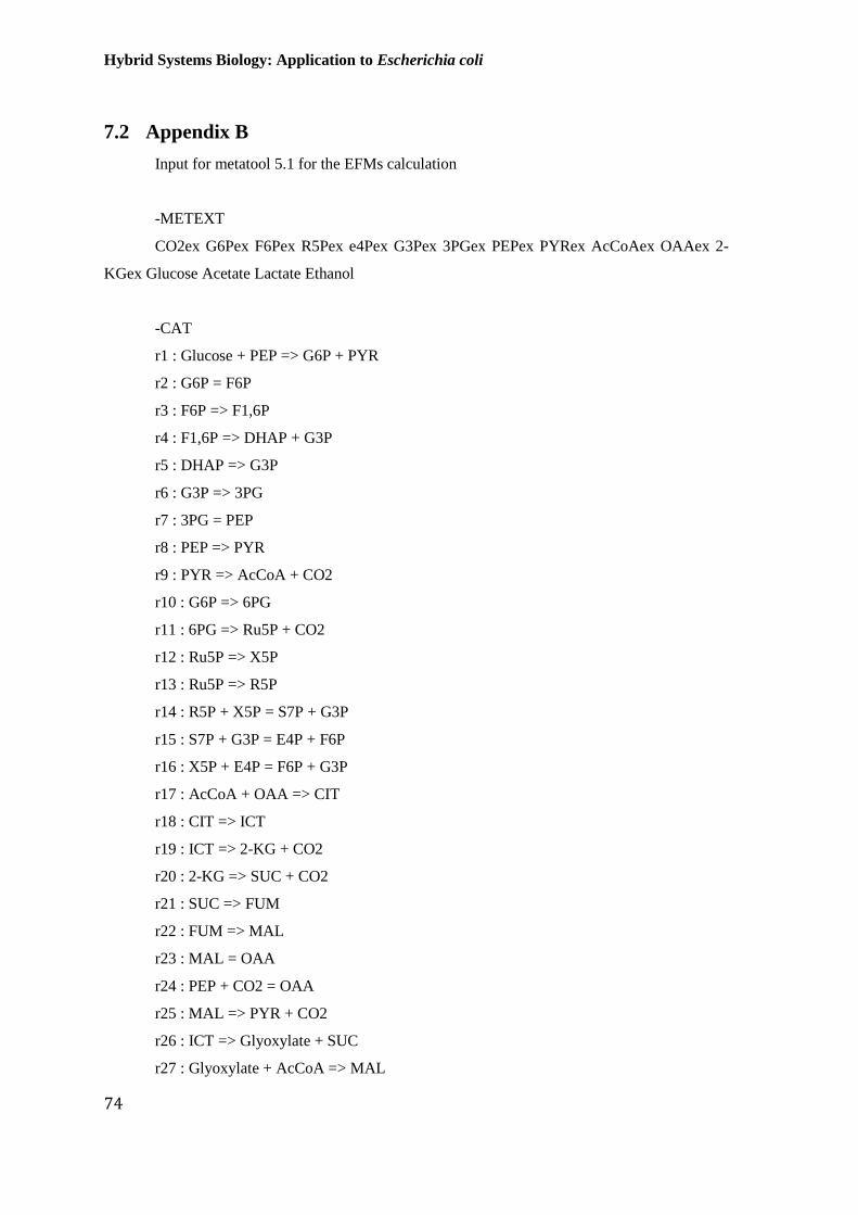
Hybrid Systems Biology: Application to Escherichia coli
74
7.2 Appendix B
Input for metatool 5.1 for the EFMs calculation
-METEXT
CO2ex G6Pex F6Pex R5Pex e4Pex G3Pex 3PGex PEPex PYRex AcCoAex OAAex 2-
KGex Glucose Acetate Lactate Ethanol
-CAT
r1 : Glucose + PEP => G6P + PYR
r2 : G6P = F6P
r3 : F6P => F1,6P
r4 : F1,6P => DHAP + G3P
r5 : DHAP => G3P
r6 : G3P => 3PG
r7 : 3PG = PEP
r8 : PEP => PYR
r9 : PYR => AcCoA + CO2
r10 : G6P => 6PG
r11 : 6PG => Ru5P + CO2
r12 : Ru5P => X5P
r13 : Ru5P => R5P
r14 : R5P + X5P = S7P + G3P
r15 : S7P + G3P = E4P + F6P
r16 : X5P + E4P = F6P + G3P
r17 : AcCoA + OAA => CIT
r18 : CIT => ICT
r19 : ICT => 2-KG + CO2
r20 : 2-KG => SUC + CO2
r21 : SUC => FUM
r22 : FUM => MAL
r23 : MAL = OAA
r24 : PEP + CO2 = OAA
r25 : MAL => PYR + CO2
r26 : ICT => Glyoxylate + SUC
r27 : Glyoxylate + AcCoA => MAL

7. Appendix
75
r28 : 6PG => G3P + PYR
r29 : AcCoA => Acetate
r30 : PYR => Lactate
r31 : AcCoA => Ethanol
r32 : G6P => G6Pex
r33 : F6P => F6Pex
r34 : R5P => R5Pex
r35 : E4P => E4Pex
r36 : G3P => G3Pex
r37 : 3PG => 3PGex
r38 : PEP => PEPex
r39 : PYR => PYRex
r40 : AcCoA => AcCoAex
r41 : OAA => OAAex
r42 : 2-KG => 2-KGex
r43 : CO2 => CO2ex
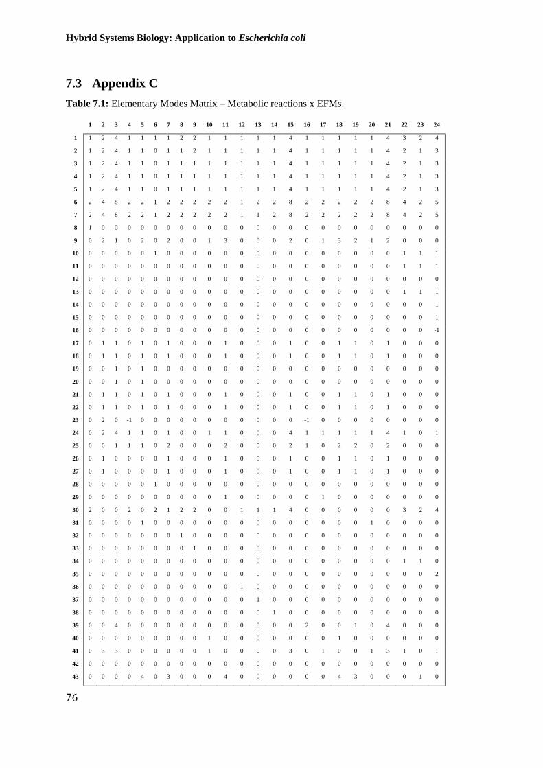
Hybrid Systems Biology: Application to Escherichia coli
76
7.3 Appendix C
Table 7.1: Elementary Modes Matrix – Metabolic reactions x EFMs.
1 2 3 4 5 6 7 8 9 10 11 12 13 14 15 16 17 18 19 20 21 22 23 24
1 1 2 4 1 1 1 1 2 2 1 1 1 1 1 4 1 1 1 1 1 4 3 2 4
2 1 2 4 1 1 0 1 1 2 1 1 1 1 1 4 1 1 1 1 1 4 2 1 3
3 1 2 4 1 1 0 1 1 1 1 1 1 1 1 4 1 1 1 1 1 4 2 1 3
4 1 2 4 1 1 0 1 1 1 1 1 1 1 1 4 1 1 1 1 1 4 2 1 3
5 1 2 4 1 1 0 1 1 1 1 1 1 1 1 4 1 1 1 1 1 4 2 1 3
6 2 4 8 2 2 1 2 2 2 2 2 1 2 2 8 2 2 2 2 2 8 4 2 5
7 2 4 8 2 2 1 2 2 2 2 2 1 1 2 8 2 2 2 2 2 8 4 2 5
8 1 0 0 0 0 0 0 0 0 0 0 0 0 0 0 0 0 0 0 0 0 0 0 0
9 0 2 1 0 2 0 2 0 0 1 3 0 0 0 2 0 1 3 2 1 2 0 0 0
10 0 0 0 0 0 1 0 0 0 0 0 0 0 0 0 0 0 0 0 0 0 1 1 1
11 0 0 0 0 0 0 0 0 0 0 0 0 0 0 0 0 0 0 0 0 0 1 1 1
12 0 0 0 0 0 0 0 0 0 0 0 0 0 0 0 0 0 0 0 0 0 0 0 0
13 0 0 0 0 0 0 0 0 0 0 0 0 0 0 0 0 0 0 0 0 0 1 1 1
14 0 0 0 0 0 0 0 0 0 0 0 0 0 0 0 0 0 0 0 0 0 0 0 1
15 0 0 0 0 0 0 0 0 0 0 0 0 0 0 0 0 0 0 0 0 0 0 0 1
16 0 0 0 0 0 0 0 0 0 0 0 0 0 0 0 0 0 0 0 0 0 0 0 -1
17 0 1 1 0 1 0 1 0 0 0 1 0 0 0 1 0 0 1 1 0 1 0 0 0
18 0 1 1 0 1 0 1 0 0 0 1 0 0 0 1 0 0 1 1 0 1 0 0 0
19 0 0 1 0 1 0 0 0 0 0 0 0 0 0 0 0 0 0 0 0 0 0 0 0
20 0 0 1 0 1 0 0 0 0 0 0 0 0 0 0 0 0 0 0 0 0 0 0 0
21 0 1 1 0 1 0 1 0 0 0 1 0 0 0 1 0 0 1 1 0 1 0 0 0
22 0 1 1 0 1 0 1 0 0 0 1 0 0 0 1 0 0 1 1 0 1 0 0 0
23 0 2 0 -1 0 0 0 0 0 0 0 0 0 0 0 -1 0 0 0 0 0 0 0 0
24 0 2 4 1 1 0 1 0 0 1 1 0 0 0 4 1 1 1 1 1 4 1 0 1
25 0 0 1 1 1 0 2 0 0 0 2 0 0 0 2 1 0 2 2 0 2 0 0 0
26 0 1 0 0 0 0 1 0 0 0 1 0 0 0 1 0 0 1 1 0 1 0 0 0
27 0 1 0 0 0 0 1 0 0 0 1 0 0 0 1 0 0 1 1 0 1 0 0 0
28 0 0 0 0 0 1 0 0 0 0 0 0 0 0 0 0 0 0 0 0 0 0 0 0
29 0 0 0 0 0 0 0 0 0 0 1 0 0 0 0 0 1 0 0 0 0 0 0 0
30 2 0 0 2 0 2 1 2 2 0 0 1 1 1 4 0 0 0 0 0 0 3 2 4
31 0 0 0 0 1 0 0 0 0 0 0 0 0 0 0 0 0 0 0 1 0 0 0 0
32 0 0 0 0 0 0 0 1 0 0 0 0 0 0 0 0 0 0 0 0 0 0 0 0
33 0 0 0 0 0 0 0 0 1 0 0 0 0 0 0 0 0 0 0 0 0 0 0 0
34 0 0 0 0 0 0 0 0 0 0 0 0 0 0 0 0 0 0 0 0 0 1 1 0
35 0 0 0 0 0 0 0 0 0 0 0 0 0 0 0 0 0 0 0 0 0 0 0 2
36 0 0 0 0 0 0 0 0 0 0 0 1 0 0 0 0 0 0 0 0 0 0 0 0
37 0 0 0 0 0 0 0 0 0 0 0 0 1 0 0 0 0 0 0 0 0 0 0 0
38 0 0 0 0 0 0 0 0 0 0 0 0 0 1 0 0 0 0 0 0 0 0 0 0
39 0 0 4 0 0 0 0 0 0 0 0 0 0 0 0 2 0 0 1 0 4 0 0 0
40 0 0 0 0 0 0 0 0 0 1 0 0 0 0 0 0 0 1 0 0 0 0 0 0
41 0 3 3 0 0 0 0 0 0 1 0 0 0 0 3 0 1 0 0 1 3 1 0 1
42 0 0 0 0 0 0 0 0 0 0 0 0 0 0 0 0 0 0 0 0 0 0 0 0
43 0 0 0 0 4 0 3 0 0 0 4 0 0 0 0 0 0 4 3 0 0 0 1 0

7. Appendix
77
Table 7.1 (cont.): Elementary Modes Matrix – Metabolic reactions x EFMs.
25 26 27 28 29 30 31 32 33 34 35 36 37 38 39 40 41 42 43 44 45 46 47 48
1 3 4 1 1 2 4 2 1 3 3 2 2 2 1 1 2 4 2 4 1 2 2 1 1
2 2 1 -2 1 0 -2 2 1 3 -2 0 0 0 1 0 0 2 0 2 0 1 2 1 1
3 2 3 0 1 1 1 2 1 3 0 1 1 1 1 0 1 3 1 3 0 1 1 1 1
4 2 3 0 1 1 1 2 1 3 0 1 1 1 1 0 1 3 1 3 0 1 1 1 1
5 2 3 0 1 1 1 2 1 3 0 1 1 1 1 0 1 3 1 3 0 1 1 1 1
6 3 7 1 2 2 2 4 2 6 1 2 2 2 2 0 2 6 2 6 1 2 2 1 2
7 3 7 1 2 2 2 4 2 6 1 2 2 2 2 0 2 6 2 6 1 2 2 1 1
8 0 0 0 0 0 0 0 0 0 0 0 0 0 1 0 0 0 0 0 0 0 0 0 0
9 0 0 0 3 2 4 1 1 1 4 2 2 2 0 2 0 0 0 0 0 0 0 0 0
10 1 3 3 0 2 6 0 0 0 5 2 2 2 0 1 2 2 2 2 1 0 0 0 0
11 1 3 3 0 2 6 0 0 0 4 2 2 2 0 0 2 2 2 2 0 0 0 0 0
12 0 2 2 0 1 3 0 0 0 2 1 1 1 0 0 1 1 1 1 0 0 0 0 0
13 1 1 1 0 1 3 0 0 0 2 1 1 1 0 0 1 1 1 1 0 0 0 0 0
14 1 1 1 0 1 3 0 0 0 2 1 1 1 0 0 1 1 1 1 0 0 0 0 0
15 1 1 1 0 1 3 0 0 0 2 1 1 1 0 0 1 1 1 1 0 0 0 0 0
16 -1 1 1 0 0 0 0 0 0 0 0 0 0 0 0 0 0 0 0 0 0 0 0 0
17 0 0 0 1 2 2 1 1 1 2 0 0 0 0 1 0 0 0 0 0 0 0 0 0
18 0 0 0 1 2 2 1 1 1 2 0 0 0 0 1 0 0 0 0 0 0 0 0 0
19 0 0 0 0 2 0 1 1 1 0 0 0 0 0 0 0 0 0 0 0 0 0 0 0
20 0 0 0 0 2 0 0 0 1 0 0 0 0 0 0 0 0 0 0 0 0 0 0 0
21 0 0 0 1 2 2 0 0 1 2 0 0 0 0 1 0 0 0 0 0 0 0 0 0
22 0 0 0 1 2 2 0 0 1 2 0 0 0 0 1 0 0 0 0 0 0 0 0 0
23 0 0 0 0 2 4 0 0 1 4 0 0 0 0 2 0 0 0 0 0 0 0 0 0
24 0 3 0 1 0 -2 2 1 3 -2 0 0 0 0 -1 0 2 0 2 0 0 0 0 0
25 0 0 0 2 0 0 0 0 0 0 0 0 0 0 0 0 0 0 0 0 0 0 0 0
26 0 0 0 1 0 2 0 0 0 2 0 0 0 0 1 0 0 0 0 0 0 0 0 0
27 0 0 0 1 0 2 0 0 0 2 0 0 0 0 1 0 0 0 0 0 0 0 0 0
28 0 0 0 0 0 0 0 0 0 1 0 0 0 0 1 0 0 0 0 1 0 0 0 0
29 0 0 0 0 0 0 0 0 0 0 2 0 0 0 0 0 0 0 0 0 0 0 0 0
30 3 4 1 0 0 0 1 0 2 0 0 0 0 0 0 2 4 0 0 0 0 0 0 0
31 0 0 0 1 0 0 0 0 0 0 0 0 2 0 0 0 0 0 0 0 0 0 0 0
32 0 0 0 0 0 0 0 0 0 0 0 0 0 0 0 0 0 0 0 0 1 0 0 0
33 0 0 0 0 0 0 0 0 0 0 0 0 0 0 0 0 0 0 0 0 0 1 0 0
34 0 0 0 0 0 0 0 0 0 0 0 0 0 0 0 0 0 0 0 0 0 0 0 0
35 2 0 0 0 1 3 0 0 0 2 1 1 1 0 0 1 1 1 1 0 0 0 0 0
36 0 0 0 0 0 0 0 0 0 0 0 0 0 0 1 0 0 0 0 0 0 0 1 0
37 0 0 0 0 0 0 0 0 0 0 0 0 0 0 0 0 0 0 0 0 0 0 0 1
38 0 0 0 0 0 0 0 0 0 0 0 0 0 0 0 0 0 0 0 0 0 0 0 0
39 0 0 0 0 0 0 0 0 0 0 0 0 0 2 0 0 0 2 4 2 2 2 1 1
40 0 0 0 0 0 0 0 0 0 0 0 2 0 0 0 0 0 0 0 0 0 0 0 0
41 0 3 0 0 0 0 1 0 3 0 0 0 0 0 0 0 2 0 2 0 0 0 0 0
42 0 0 0 0 0 0 1 1 0 0 0 0 0 0 0 0 0 0 0 0 0 0 0 0
43 1 0 3 4 8 12 0 1 0 10 4 4 4 0 3 2 0 2 0 0 0 0 0 0

Hybrid Systems Biology: Application to Escherichia coli
78
Table 7.1(cont.): Elementary Modes Matrix – Metabolic reactions x EFMs.
49 50 51 52 53 54 55 56 57 58 59 60 61 62 63 64 65 66 67 68 69 70 71 72
1 1 1 1 1 1 1 1 1 1 1 2 2 1 1 1 2 2 2 2 1 1 1 1 1
2 1 1 1 1 1 1 1 0 0 0 1 2 1 1 1 1 1 2 2 1 1 1 1 1
3 1 1 1 1 1 1 1 0 0 0 1 1 1 1 1 1 1 1 1 1 1 1 1 1
4 1 1 1 1 1 1 1 0 0 0 1 1 1 1 1 1 1 1 1 1 1 1 1 1
5 1 1 1 1 1 1 1 0 0 0 1 1 1 1 1 1 1 1 1 1 1 1 1 1
6 2 2 2 2 2 2 2 1 1 1 2 2 1 2 2 2 2 2 2 1 1 2 2 2
7 2 2 2 2 2 2 2 1 1 1 2 2 1 1 2 2 2 2 2 1 1 1 1 2
8 0 1 1 1 0 0 0 0 0 0 0 0 0 0 0 0 0 0 0 0 0 0 0 0
9 0 2 2 2 2 2 2 2 2 2 2 2 1 1 1 2 2 2 2 1 1 1 1 1
10 0 0 0 0 0 0 0 1 1 1 0 0 0 0 0 0 0 0 0 0 0 0 0 0
11 0 0 0 0 0 0 0 0 0 0 0 0 0 0 0 0 0 0 0 0 0 0 0 0
12 0 0 0 0 0 0 0 0 0 0 0 0 0 0 0 0 0 0 0 0 0 0 0 0
13 0 0 0 0 0 0 0 0 0 0 0 0 0 0 0 0 0 0 0 0 0 0 0 0
14 0 0 0 0 0 0 0 0 0 0 0 0 0 0 0 0 0 0 0 0 0 0 0 0
15 0 0 0 0 0 0 0 0 0 0 0 0 0 0 0 0 0 0 0 0 0 0 0 0
16 0 0 0 0 0 0 0 0 0 0 0 0 0 0 0 0 0 0 0 0 0 0 0 0
17 0 0 0 0 0 0 0 0 0 0 0 0 0 0 0 0 0 0 0 0 0 0 0 0
18 0 0 0 0 0 0 0 0 0 0 0 0 0 0 0 0 0 0 0 0 0 0 0 0
19 0 0 0 0 0 0 0 0 0 0 0 0 0 0 0 0 0 0 0 0 0 0 0 0
20 0 0 0 0 0 0 0 0 0 0 0 0 0 0 0 0 0 0 0 0 0 0 0 0
21 0 0 0 0 0 0 0 0 0 0 0 0 0 0 0 0 0 0 0 0 0 0 0 0
22 0 0 0 0 0 0 0 0 0 0 0 0 0 0 0 0 0 0 0 0 0 0 0 0
23 0 0 0 0 -1 -1 -1 0 0 0 0 0 0 0 0 0 0 0 0 0 0 0 0 0
24 0 0 0 0 1 1 1 0 0 0 0 0 0 0 0 0 0 0 0 0 0 0 0 0
25 0 0 0 0 1 1 1 0 0 0 0 0 0 0 0 0 0 0 0 0 0 0 0 0
26 0 0 0 0 0 0 0 0 0 0 0 0 0 0 0 0 0 0 0 0 0 0 0 0
27 0 0 0 0 0 0 0 0 0 0 0 0 0 0 0 0 0 0 0 0 0 0 0 0
28 0 0 0 0 0 0 0 1 1 1 0 0 0 0 0 0 0 0 0 0 0 0 0 0
29 0 0 0 2 0 0 2 0 0 2 0 0 0 0 0 0 2 0 2 0 1 0 1 0
30 0 0 0 0 0 0 0 0 0 0 0 0 0 0 0 0 0 0 0 0 0 0 0 0
31 0 2 0 0 2 0 0 2 0 0 2 2 1 1 1 0 0 0 0 0 0 0 0 0
32 0 0 0 0 0 0 0 0 0 0 1 0 0 0 0 1 1 0 0 0 0 0 0 0
33 0 0 0 0 0 0 0 0 0 0 0 1 0 0 0 0 0 1 1 0 0 0 0 0
34 0 0 0 0 0 0 0 0 0 0 0 0 0 0 0 0 0 0 0 0 0 0 0 0
35 0 0 0 0 0 0 0 0 0 0 0 0 0 0 0 0 0 0 0 0 0 0 0 0
36 0 0 0 0 0 0 0 0 0 0 0 0 1 0 0 0 0 0 0 1 1 0 0 0
37 0 0 0 0 0 0 0 0 0 0 0 0 0 1 0 0 0 0 0 0 0 1 1 0
38 1 0 0 0 0 0 0 0 0 0 0 0 0 0 1 0 0 0 0 0 0 0 0 1
39 1 0 0 0 0 0 0 0 0 0 0 0 0 0 0 0 0 0 0 0 0 0 0 0
40 0 0 2 0 0 2 0 0 2 0 0 0 0 0 0 2 0 2 0 1 0 1 0 1
41 0 0 0 0 0 0 0 0 0 0 0 0 0 0 0 0 0 0 0 0 0 0 0 0
42 0 0 0 0 0 0 0 0 0 0 0 0 0 0 0 0 0 0 0 0 0 0 0 0
43 0 2 2 2 2 2 2 2 2 2 2 2 1 1 1 2 2 2 2 1 1 1 1 1
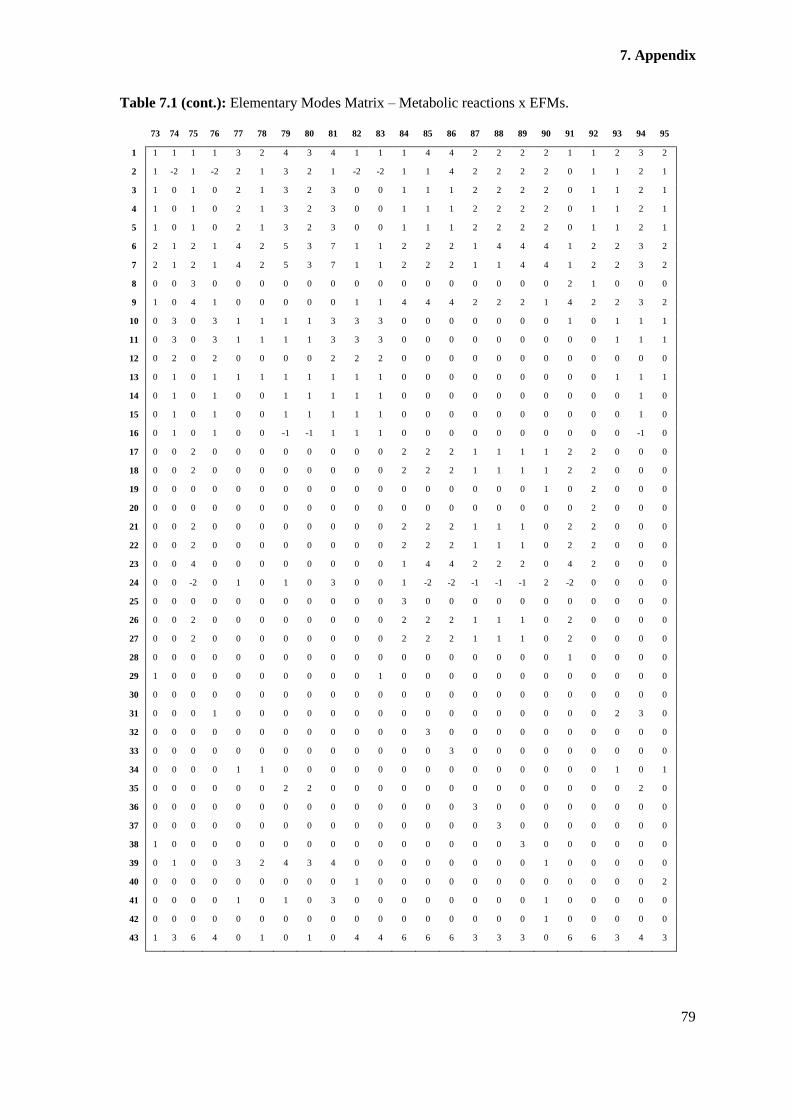
7. Appendix
79
Table 7.1 (cont.): Elementary Modes Matrix – Metabolic reactions x EFMs.
73 74 75 76 77 78 79 80 81 82 83 84 85 86 87 88 89 90 91 92 93 94 95
1 1 1 1 1 3 2 4 3 4 1 1 1 4 4 2 2 2 2 1 1 2 3 2
2 1 -2 1 -2 2 1 3 2 1 -2 -2 1 1 4 2 2 2 2 0 1 1 2 1
3 1 0 1 0 2 1 3 2 3 0 0 1 1 1 2 2 2 2 0 1 1 2 1
4 1 0 1 0 2 1 3 2 3 0 0 1 1 1 2 2 2 2 0 1 1 2 1
5 1 0 1 0 2 1 3 2 3 0 0 1 1 1 2 2 2 2 0 1 1 2 1
6 2 1 2 1 4 2 5 3 7 1 1 2 2 2 1 4 4 4 1 2 2 3 2
7 2 1 2 1 4 2 5 3 7 1 1 2 2 2 1 1 4 4 1 2 2 3 2
8 0 0 3 0 0 0 0 0 0 0 0 0 0 0 0 0 0 0 2 1 0 0 0
9 1 0 4 1 0 0 0 0 0 1 1 4 4 4 2 2 2 1 4 2 2 3 2
10 0 3 0 3 1 1 1 1 3 3 3 0 0 0 0 0 0 0 1 0 1 1 1
11 0 3 0 3 1 1 1 1 3 3 3 0 0 0 0 0 0 0 0 0 1 1 1
12 0 2 0 2 0 0 0 0 2 2 2 0 0 0 0 0 0 0 0 0 0 0 0
13 0 1 0 1 1 1 1 1 1 1 1 0 0 0 0 0 0 0 0 0 1 1 1
14 0 1 0 1 0 0 1 1 1 1 1 0 0 0 0 0 0 0 0 0 0 1 0
15 0 1 0 1 0 0 1 1 1 1 1 0 0 0 0 0 0 0 0 0 0 1 0
16 0 1 0 1 0 0 -1 -1 1 1 1 0 0 0 0 0 0 0 0 0 0 -1 0
17 0 0 2 0 0 0 0 0 0 0 0 2 2 2 1 1 1 1 2 2 0 0 0
18 0 0 2 0 0 0 0 0 0 0 0 2 2 2 1 1 1 1 2 2 0 0 0
19 0 0 0 0 0 0 0 0 0 0 0 0 0 0 0 0 0 1 0 2 0 0 0
20 0 0 0 0 0 0 0 0 0 0 0 0 0 0 0 0 0 0 0 2 0 0 0
21 0 0 2 0 0 0 0 0 0 0 0 2 2 2 1 1 1 0 2 2 0 0 0
22 0 0 2 0 0 0 0 0 0 0 0 2 2 2 1 1 1 0 2 2 0 0 0
23 0 0 4 0 0 0 0 0 0 0 0 1 4 4 2 2 2 0 4 2 0 0 0
24 0 0 -2 0 1 0 1 0 3 0 0 1 -2 -2 -1 -1 -1 2 -2 0 0 0 0
25 0 0 0 0 0 0 0 0 0 0 0 3 0 0 0 0 0 0 0 0 0 0 0
26 0 0 2 0 0 0 0 0 0 0 0 2 2 2 1 1 1 0 2 0 0 0 0
27 0 0 2 0 0 0 0 0 0 0 0 2 2 2 1 1 1 0 2 0 0 0 0
28 0 0 0 0 0 0 0 0 0 0 0 0 0 0 0 0 0 0 1 0 0 0 0
29 1 0 0 0 0 0 0 0 0 0 1 0 0 0 0 0 0 0 0 0 0 0 0
30 0 0 0 0 0 0 0 0 0 0 0 0 0 0 0 0 0 0 0 0 0 0 0
31 0 0 0 1 0 0 0 0 0 0 0 0 0 0 0 0 0 0 0 0 2 3 0
32 0 0 0 0 0 0 0 0 0 0 0 0 3 0 0 0 0 0 0 0 0 0 0
33 0 0 0 0 0 0 0 0 0 0 0 0 0 3 0 0 0 0 0 0 0 0 0
34 0 0 0 0 1 1 0 0 0 0 0 0 0 0 0 0 0 0 0 0 1 0 1
35 0 0 0 0 0 0 2 2 0 0 0 0 0 0 0 0 0 0 0 0 0 2 0
36 0 0 0 0 0 0 0 0 0 0 0 0 0 0 3 0 0 0 0 0 0 0 0
37 0 0 0 0 0 0 0 0 0 0 0 0 0 0 0 3 0 0 0 0 0 0 0
38 1 0 0 0 0 0 0 0 0 0 0 0 0 0 0 0 3 0 0 0 0 0 0
39 0 1 0 0 3 2 4 3 4 0 0 0 0 0 0 0 0 1 0 0 0 0 0
40 0 0 0 0 0 0 0 0 0 1 0 0 0 0 0 0 0 0 0 0 0 0 2
41 0 0 0 0 1 0 1 0 3 0 0 0 0 0 0 0 0 1 0 0 0 0 0
42 0 0 0 0 0 0 0 0 0 0 0 0 0 0 0 0 0 1 0 0 0 0 0
43 1 3 6 4 0 1 0 1 0 4 4 6 6 6 3 3 3 0 6 6 3 4 3
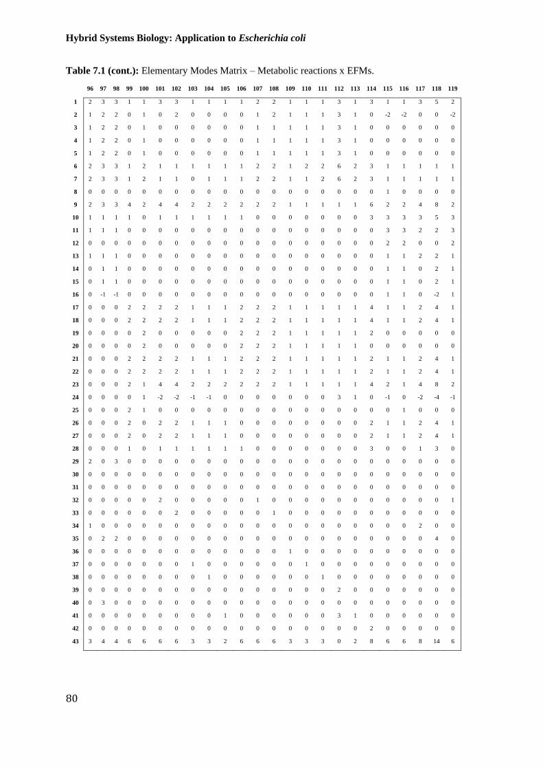
Hybrid Systems Biology: Application to Escherichia coli
80
Table 7.1 (cont.): Elementary Modes Matrix – Metabolic reactions x EFMs.
96 97 98 99 100 101 102 103 104 105 106 107 108 109 110 111 112 113 114 115 116 117 118 119
1 2 3 3 1 1 3 3 1 1 1 1 2 2 1 1 1 3 1 3 1 1 3 5 2
2 1 2 2 0 1 0 2 0 0 0 0 1 2 1 1 1 3 1 0 -2 -2 0 0 -2
3 1 2 2 0 1 0 0 0 0 0 0 1 1 1 1 1 3 1 0 0 0 0 0 0
4 1 2 2 0 1 0 0 0 0 0 0 1 1 1 1 1 3 1 0 0 0 0 0 0
5 1 2 2 0 1 0 0 0 0 0 0 1 1 1 1 1 3 1 0 0 0 0 0 0
6 2 3 3 1 2 1 1 1 1 1 1 2 2 1 2 2 6 2 3 1 1 1 1 1
7 2 3 3 1 2 1 1 0 1 1 1 2 2 1 1 2 6 2 3 1 1 1 1 1
8 0 0 0 0 0 0 0 0 0 0 0 0 0 0 0 0 0 0 0 1 0 0 0 0
9 2 3 3 4 2 4 4 2 2 2 2 2 2 1 1 1 1 1 6 2 2 4 8 2
10 1 1 1 1 0 1 1 1 1 1 1 0 0 0 0 0 0 0 3 3 3 3 5 3
11 1 1 1 0 0 0 0 0 0 0 0 0 0 0 0 0 0 0 0 3 3 2 2 3
12 0 0 0 0 0 0 0 0 0 0 0 0 0 0 0 0 0 0 0 2 2 0 0 2
13 1 1 1 0 0 0 0 0 0 0 0 0 0 0 0 0 0 0 0 1 1 2 2 1
14 0 1 1 0 0 0 0 0 0 0 0 0 0 0 0 0 0 0 0 1 1 0 2 1
15 0 1 1 0 0 0 0 0 0 0 0 0 0 0 0 0 0 0 0 1 1 0 2 1
16 0 -1 -1 0 0 0 0 0 0 0 0 0 0 0 0 0 0 0 0 1 1 0 -2 1
17 0 0 0 2 2 2 2 1 1 1 2 2 2 1 1 1 1 1 4 1 1 2 4 1
18 0 0 0 2 2 2 2 1 1 1 2 2 2 1 1 1 1 1 4 1 1 2 4 1
19 0 0 0 0 2 0 0 0 0 0 2 2 2 1 1 1 1 1 2 0 0 0 0 0
20 0 0 0 0 2 0 0 0 0 0 2 2 2 1 1 1 1 1 0 0 0 0 0 0
21 0 0 0 2 2 2 2 1 1 1 2 2 2 1 1 1 1 1 2 1 1 2 4 1
22 0 0 0 2 2 2 2 1 1 1 2 2 2 1 1 1 1 1 2 1 1 2 4 1
23 0 0 0 2 1 4 4 2 2 2 2 2 2 1 1 1 1 1 4 2 1 4 8 2
24 0 0 0 0 1 -2 -2 -1 -1 0 0 0 0 0 0 0 3 1 0 -1 0 -2 -4 -1
25 0 0 0 2 1 0 0 0 0 0 0 0 0 0 0 0 0 0 0 0 1 0 0 0
26 0 0 0 2 0 2 2 1 1 1 0 0 0 0 0 0 0 0 2 1 1 2 4 1
27 0 0 0 2 0 2 2 1 1 1 0 0 0 0 0 0 0 0 2 1 1 2 4 1
28 0 0 0 1 0 1 1 1 1 1 1 0 0 0 0 0 0 0 3 0 0 1 3 0
29 2 0 3 0 0 0 0 0 0 0 0 0 0 0 0 0 0 0 0 0 0 0 0 0
30 0 0 0 0 0 0 0 0 0 0 0 0 0 0 0 0 0 0 0 0 0 0 0 0
31 0 0 0 0 0 0 0 0 0 0 0 0 0 0 0 0 0 0 0 0 0 0 0 0
32 0 0 0 0 0 2 0 0 0 0 0 1 0 0 0 0 0 0 0 0 0 0 0 1
33 0 0 0 0 0 0 2 0 0 0 0 0 1 0 0 0 0 0 0 0 0 0 0 0
34 1 0 0 0 0 0 0 0 0 0 0 0 0 0 0 0 0 0 0 0 0 2 0 0
35 0 2 2 0 0 0 0 0 0 0 0 0 0 0 0 0 0 0 0 0 0 0 4 0
36 0 0 0 0 0 0 0 0 0 0 0 0 0 1 0 0 0 0 0 0 0 0 0 0
37 0 0 0 0 0 0 0 1 0 0 0 0 0 0 1 0 0 0 0 0 0 0 0 0
38 0 0 0 0 0 0 0 0 1 0 0 0 0 0 0 1 0 0 0 0 0 0 0 0
39 0 0 0 0 0 0 0 0 0 0 0 0 0 0 0 0 2 0 0 0 0 0 0 0
40 0 3 0 0 0 0 0 0 0 0 0 0 0 0 0 0 0 0 0 0 0 0 0 0
41 0 0 0 0 0 0 0 0 0 1 0 0 0 0 0 0 3 1 0 0 0 0 0 0
42 0 0 0 0 0 0 0 0 0 0 0 0 0 0 0 0 0 0 2 0 0 0 0 0
43 3 4 4 6 6 6 6 3 3 2 6 6 6 3 3 3 0 2 8 6 6 8 14 6

7. Appendix
81
Table 7.1 (cont.): Elementary Modes Matrix – Metabolic reactions x EFMs.
120 121 122 123 124 125 126 127 128 129 130 131 132 133 134 135 136 137 138 139 140 141 142 143 144 145
1 2 2 4 2 2 2 2 2 2 1 3 2 3 1 1 4 1 1 1 1 2 2 1 1 1 2
2 -1 -2 1 -3 1 -4 -4 -4 -4 -2 -6 1 2 1 1 4 1 1 1 1 1 2 1 1 1 1
3 0 0 1 0 1 0 0 0 0 0 0 1 2 1 1 4 1 1 1 1 1 1 1 1 1 1
4 0 0 1 0 1 0 0 0 0 0 0 1 2 1 1 4 1 1 1 1 1 1 1 1 1 1
5 0 0 1 0 1 0 0 0 0 0 0 1 2 1 1 4 1 1 1 1 1 1 1 1 1 1
6 1 1 2 1 1 1 2 2 2 1 3 2 3 2 2 8 2 2 2 2 2 2 1 2 2 2
7 1 1 2 1 1 1 1 2 2 1 3 2 3 2 2 8 2 2 2 2 2 2 1 1 2 2
8 0 0 0 0 0 0 0 0 0 0 0 0 0 0 0 0 0 0 1 1 0 0 0 0 0 0
9 2 2 4 2 2 2 2 2 2 1 3 2 3 1 2 1 2 1 4 2 4 4 2 2 2 2
10 3 4 3 5 1 6 6 6 6 3 9 1 1 0 0 0 0 0 0 0 0 0 0 0 0 0
11 3 4 3 5 1 6 6 6 6 3 9 1 1 0 0 0 0 0 0 0 0 0 0 0 0 0
12 2 2 0 3 0 4 4 4 4 2 6 0 0 0 0 0 0 0 0 0 0 0 0 0 0 0
13 1 2 3 2 1 2 2 2 2 1 3 1 1 0 0 0 0 0 0 0 0 0 0 0 0 0
14 1 1 0 2 1 2 2 2 2 1 3 0 1 0 0 0 0 0 0 0 0 0 0 0 0 0
15 1 1 0 2 1 2 2 2 2 1 3 0 1 0 0 0 0 0 0 0 0 0 0 0 0 0
16 1 1 0 1 -1 2 2 2 2 1 3 0 -1 0 0 0 0 0 0 0 0 0 0 0 0 0
17 1 1 2 1 1 1 1 1 1 1 2 2 3 1 1 1 1 1 2 1 2 2 1 1 1 1
18 1 1 2 1 1 1 1 1 1 1 2 2 3 1 1 1 1 1 2 1 2 2 1 1 1 1
19 0 0 0 0 0 0 0 0 0 1 1 2 3 1 1 1 1 1 0 0 0 0 0 0 0 0
20 0 0 0 0 0 0 0 0 0 1 0 2 3 1 1 1 1 1 0 0 0 0 0 0 0 0
21 1 1 2 1 1 1 1 1 1 1 1 2 3 1 1 1 1 1 2 1 2 2 1 1 1 1
22 1 1 2 1 1 1 1 1 1 1 1 2 3 1 1 1 1 1 2 1 2 2 1 1 1 1
23 2 2 4 2 2 2 2 2 2 1 2 2 3 0 0 0 0 0 2 2 2 2 1 1 1 2
24 -1 -1 -2 -1 -1 -1 -1 -1 0 0 0 0 0 1 1 4 1 1 0 0 0 0 0 0 0 0
25 0 0 0 0 0 0 0 0 0 0 0 0 0 1 1 1 1 1 2 0 2 2 1 1 1 0
26 1 1 2 1 1 1 1 1 1 0 1 0 0 0 0 0 0 0 2 1 2 2 1 1 1 1
27 1 1 2 1 1 1 1 1 1 0 1 0 0 0 0 0 0 0 2 1 2 2 1 1 1 1
28 0 0 0 0 0 0 0 0 0 0 0 0 0 0 0 0 0 0 0 0 0 0 0 0 0 0
29 0 0 0 0 0 0 0 0 0 0 0 0 0 0 0 0 1 0 0 0 0 0 0 0 0 0
30 0 0 0 0 0 0 0 0 0 0 0 0 0 0 0 4 0 1 0 0 0 0 0 0 0 0
31 0 0 0 0 0 0 0 0 0 0 0 0 0 0 0 0 0 0 0 0 0 0 0 0 0 0
32 0 0 0 0 0 0 0 0 0 0 0 0 0 0 0 0 0 0 0 0 1 0 0 0 0 1
33 1 0 0 0 0 0 0 0 0 0 0 0 0 0 0 0 0 0 0 0 0 1 0 0 0 0
34 0 1 3 0 0 0 0 0 0 0 0 1 0 0 0 0 0 0 0 0 0 0 0 0 0 0
35 0 0 0 1 2 0 0 0 0 0 0 0 2 0 0 0 0 0 0 0 0 0 0 0 0 0
36 0 0 0 0 0 1 0 0 0 0 0 0 0 0 0 0 0 0 0 0 0 0 1 0 0 0
37 0 0 0 0 0 0 1 0 0 0 0 0 0 0 0 0 0 0 0 0 0 0 0 1 0 0
38 0 0 0 0 0 0 0 1 0 0 0 0 0 0 0 0 0 0 0 0 0 0 0 0 1 0
39 0 0 0 0 0 0 0 0 0 0 0 0 0 1 0 0 0 0 0 0 0 0 0 0 0 0
40 0 0 0 0 0 0 0 0 0 0 0 0 0 0 1 0 0 0 0 0 0 0 0 0 0 0
41 0 0 0 0 0 0 0 0 1 0 0 0 0 0 0 3 0 0 0 1 0 0 0 0 0 1
42 0 0 0 0 0 0 0 0 0 0 1 0 0 0 0 0 0 0 0 0 0 0 0 0 0 0
43 6 7 9 8 4 9 9 9 8 6 13 7 10 3 4 0 4 3 6 2 6 6 3 3 3 2
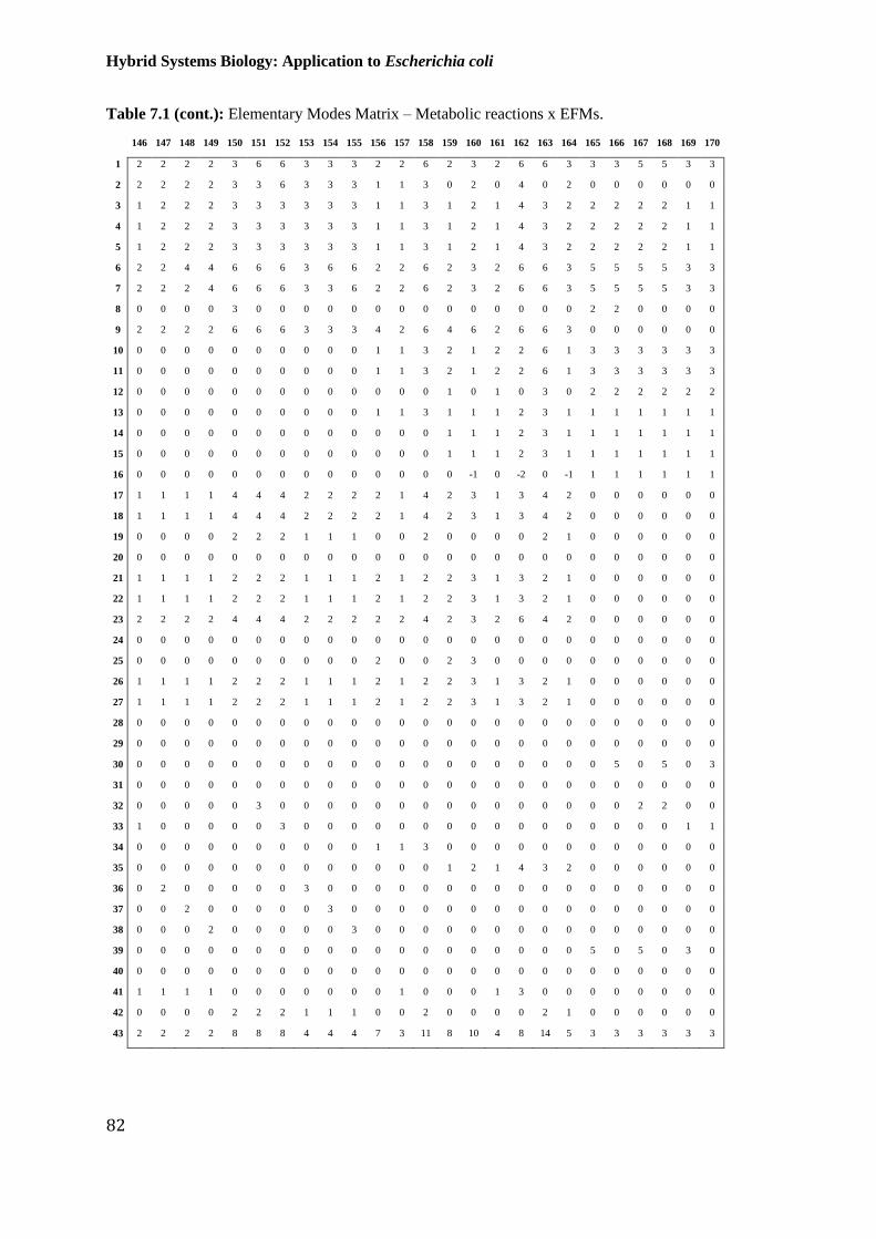
Hybrid Systems Biology: Application to Escherichia coli
82
Table 7.1 (cont.): Elementary Modes Matrix – Metabolic reactions x EFMs.
146 147 148 149 150 151 152 153 154 155 156 157 158 159 160 161 162 163 164 165 166 167 168 169 170
1 2 2 2 2 3 6 6 3 3 3 2 2 6 2 3 2 6 6 3 3 3 5 5 3 3
2 2 2 2 2 3 3 6 3 3 3 1 1 3 0 2 0 4 0 2 0 0 0 0 0 0
3 1 2 2 2 3 3 3 3 3 3 1 1 3 1 2 1 4 3 2 2 2 2 2 1 1
4 1 2 2 2 3 3 3 3 3 3 1 1 3 1 2 1 4 3 2 2 2 2 2 1 1
5 1 2 2 2 3 3 3 3 3 3 1 1 3 1 2 1 4 3 2 2 2 2 2 1 1
6 2 2 4 4 6 6 6 3 6 6 2 2 6 2 3 2 6 6 3 5 5 5 5 3 3
7 2 2 2 4 6 6 6 3 3 6 2 2 6 2 3 2 6 6 3 5 5 5 5 3 3
8 0 0 0 0 3 0 0 0 0 0 0 0 0 0 0 0 0 0 0 2 2 0 0 0 0
9 2 2 2 2 6 6 6 3 3 3 4 2 6 4 6 2 6 6 3 0 0 0 0 0 0
10 0 0 0 0 0 0 0 0 0 0 1 1 3 2 1 2 2 6 1 3 3 3 3 3 3
11 0 0 0 0 0 0 0 0 0 0 1 1 3 2 1 2 2 6 1 3 3 3 3 3 3
12 0 0 0 0 0 0 0 0 0 0 0 0 0 1 0 1 0 3 0 2 2 2 2 2 2
13 0 0 0 0 0 0 0 0 0 0 1 1 3 1 1 1 2 3 1 1 1 1 1 1 1
14 0 0 0 0 0 0 0 0 0 0 0 0 0 1 1 1 2 3 1 1 1 1 1 1 1
15 0 0 0 0 0 0 0 0 0 0 0 0 0 1 1 1 2 3 1 1 1 1 1 1 1
16 0 0 0 0 0 0 0 0 0 0 0 0 0 0 -1 0 -2 0 -1 1 1 1 1 1 1
17 1 1 1 1 4 4 4 2 2 2 2 1 4 2 3 1 3 4 2 0 0 0 0 0 0
18 1 1 1 1 4 4 4 2 2 2 2 1 4 2 3 1 3 4 2 0 0 0 0 0 0
19 0 0 0 0 2 2 2 1 1 1 0 0 2 0 0 0 0 2 1 0 0 0 0 0 0
20 0 0 0 0 0 0 0 0 0 0 0 0 0 0 0 0 0 0 0 0 0 0 0 0 0
21 1 1 1 1 2 2 2 1 1 1 2 1 2 2 3 1 3 2 1 0 0 0 0 0 0
22 1 1 1 1 2 2 2 1 1 1 2 1 2 2 3 1 3 2 1 0 0 0 0 0 0
23 2 2 2 2 4 4 4 2 2 2 2 2 4 2 3 2 6 4 2 0 0 0 0 0 0
24 0 0 0 0 0 0 0 0 0 0 0 0 0 0 0 0 0 0 0 0 0 0 0 0 0
25 0 0 0 0 0 0 0 0 0 0 2 0 0 2 3 0 0 0 0 0 0 0 0 0 0
26 1 1 1 1 2 2 2 1 1 1 2 1 2 2 3 1 3 2 1 0 0 0 0 0 0
27 1 1 1 1 2 2 2 1 1 1 2 1 2 2 3 1 3 2 1 0 0 0 0 0 0
28 0 0 0 0 0 0 0 0 0 0 0 0 0 0 0 0 0 0 0 0 0 0 0 0 0
29 0 0 0 0 0 0 0 0 0 0 0 0 0 0 0 0 0 0 0 0 0 0 0 0 0
30 0 0 0 0 0 0 0 0 0 0 0 0 0 0 0 0 0 0 0 0 5 0 5 0 3
31 0 0 0 0 0 0 0 0 0 0 0 0 0 0 0 0 0 0 0 0 0 0 0 0 0
32 0 0 0 0 0 3 0 0 0 0 0 0 0 0 0 0 0 0 0 0 0 2 2 0 0
33 1 0 0 0 0 0 3 0 0 0 0 0 0 0 0 0 0 0 0 0 0 0 0 1 1
34 0 0 0 0 0 0 0 0 0 0 1 1 3 0 0 0 0 0 0 0 0 0 0 0 0
35 0 0 0 0 0 0 0 0 0 0 0 0 0 1 2 1 4 3 2 0 0 0 0 0 0
36 0 2 0 0 0 0 0 3 0 0 0 0 0 0 0 0 0 0 0 0 0 0 0 0 0
37 0 0 2 0 0 0 0 0 3 0 0 0 0 0 0 0 0 0 0 0 0 0 0 0 0
38 0 0 0 2 0 0 0 0 0 3 0 0 0 0 0 0 0 0 0 0 0 0 0 0 0
39 0 0 0 0 0 0 0 0 0 0 0 0 0 0 0 0 0 0 0 5 0 5 0 3 0
40 0 0 0 0 0 0 0 0 0 0 0 0 0 0 0 0 0 0 0 0 0 0 0 0 0
41 1 1 1 1 0 0 0 0 0 0 0 1 0 0 0 1 3 0 0 0 0 0 0 0 0
42 0 0 0 0 2 2 2 1 1 1 0 0 2 0 0 0 0 2 1 0 0 0 0 0 0
43 2 2 2 2 8 8 8 4 4 4 7 3 11 8 10 4 8 14 5 3 3 3 3 3 3

7. Appendix
83
Table 7.1 (cont.): Elementary Modes Matrix – Metabolic reactions x EFMs.
171 172 173 174 175 176 177 178 179 180 181 182 183 184 185 186 187 188 189 190 191 192 193 194
1 5 5 3 3 3 3 3 3 3 3 3 5 3 5 3 3 3 5 5 3 3 5 5 3
2 0 0 0 0 0 0 0 0 0 0 0 0 0 0 0 0 0 0 0 0 0 0 0 0
3 2 2 2 2 2 2 2 2 2 2 2 2 1 2 2 2 2 2 2 1 1 2 2 2
4 2 2 2 2 2 2 2 2 2 2 2 2 1 2 2 2 2 2 2 1 1 2 2 2
5 2 2 2 2 2 2 2 2 2 2 2 2 1 2 2 2 2 2 2 1 1 2 2 2
6 5 5 3 3 5 5 5 5 5 5 5 5 3 5 3 5 5 5 5 3 3 5 5 3
7 5 5 3 3 3 3 5 5 5 5 5 5 3 5 3 3 5 5 5 3 3 5 5 3
8 0 0 0 0 0 0 0 0 2 2 2 0 0 0 0 0 0 0 0 0 0 0 0 0
9 0 0 0 0 0 0 0 0 5 5 5 5 3 5 3 3 3 5 5 3 3 5 5 3
10 5 5 3 3 3 3 3 3 3 3 3 3 3 5 3 3 3 3 3 3 3 5 5 3
11 5 5 3 3 3 3 3 3 3 3 3 3 3 5 3 3 3 3 3 3 3 5 5 3
12 2 2 2 2 2 2 2 2 2 2 2 2 2 2 2 2 2 2 2 2 2 2 2 2
13 3 3 1 1 1 1 1 1 1 1 1 1 1 3 1 1 1 1 1 1 1 3 3 1
14 1 1 1 1 1 1 1 1 1 1 1 1 1 1 1 1 1 1 1 1 1 1 1 1
15 1 1 1 1 1 1 1 1 1 1 1 1 1 1 1 1 1 1 1 1 1 1 1 1
16 1 1 1 1 1 1 1 1 1 1 1 1 1 1 1 1 1 1 1 1 1 1 1 1
17 0 0 0 0 0 0 0 0 0 0 0 0 0 0 0 0 0 0 0 0 0 0 0 0
18 0 0 0 0 0 0 0 0 0 0 0 0 0 0 0 0 0 0 0 0 0 0 0 0
19 0 0 0 0 0 0 0 0 0 0 0 0 0 0 0 0 0 0 0 0 0 0 0 0
20 0 0 0 0 0 0 0 0 0 0 0 0 0 0 0 0 0 0 0 0 0 0 0 0
21 0 0 0 0 0 0 0 0 0 0 0 0 0 0 0 0 0 0 0 0 0 0 0 0
22 0 0 0 0 0 0 0 0 0 0 0 0 0 0 0 0 0 0 0 0 0 0 0 0
23 0 0 0 0 0 0 0 0 0 0 0 0 0 0 0 0 0 0 0 0 0 0 0 0
24 0 0 0 0 0 0 0 0 0 0 0 0 0 0 0 0 0 0 0 0 0 0 0 0
25 0 0 0 0 0 0 0 0 0 0 0 0 0 0 0 0 0 0 0 0 0 0 0 0
26 0 0 0 0 0 0 0 0 0 0 0 0 0 0 0 0 0 0 0 0 0 0 0 0
27 0 0 0 0 0 0 0 0 0 0 0 0 0 0 0 0 0 0 0 0 0 0 0 0
28 0 0 0 0 0 0 0 0 0 0 0 0 0 0 0 0 0 0 0 0 0 0 0 0
29 0 0 0 0 0 0 0 0 0 0 5 0 0 0 0 0 0 0 5 0 3 0 5 0
30 0 5 0 3 0 3 0 3 0 0 0 0 0 0 0 0 0 0 0 0 0 0 0 0
31 0 0 0 0 0 0 0 0 5 0 0 5 3 5 3 3 3 0 0 0 0 0 0 0
32 0 0 0 0 0 0 0 0 0 0 0 2 0 0 0 0 0 2 2 0 0 0 0 0
33 0 0 0 0 0 0 0 0 0 0 0 0 1 0 0 0 0 0 0 1 1 0 0 0
34 2 2 0 0 0 0 0 0 0 0 0 0 0 2 0 0 0 0 0 0 0 2 2 0
35 0 0 0 0 0 0 0 0 0 0 0 0 0 0 0 0 0 0 0 0 0 0 0 0
36 0 0 2 2 0 0 0 0 0 0 0 0 0 0 2 0 0 0 0 0 0 0 0 2
37 0 0 0 0 2 2 0 0 0 0 0 0 0 0 0 2 0 0 0 0 0 0 0 0
38 0 0 0 0 0 0 2 2 0 0 0 0 0 0 0 0 2 0 0 0 0 0 0 0
39 5 0 3 0 3 0 3 0 0 0 0 0 0 0 0 0 0 0 0 0 0 0 0 0
40 0 0 0 0 0 0 0 0 0 5 0 0 0 0 0 0 0 5 0 3 0 5 0 3
41 0 0 0 0 0 0 0 0 0 0 0 0 0 0 0 0 0 0 0 0 0 0 0 0
42 0 0 0 0 0 0 0 0 0 0 0 0 0 0 0 0 0 0 0 0 0 0 0 0
43 5 5 3 3 3 3 3 3 8 8 8 8 6 10 6 6 6 8 8 6 6 10 10 6
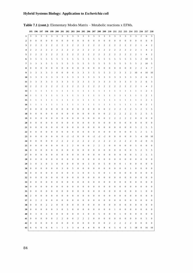
Hybrid Systems Biology: Application to Escherichia coli
84
Table 7.1 (cont.): Elementary Modes Matrix – Metabolic reactions x EFMs.
195 196 197 198 199 200 201 202 203 204 205 206 207 208 209 210 211 212 213 214 215 216 217 218
1 3 3 3 3 3 3 3 3 3 3 3 3 3 3 3 3 3 3 3 3 3 2 6 3
2 0 0 0 0 0 0 0 0 0 0 0 0 0 0 0 0 0 0 0 0 0 0 0 0
3 2 2 2 2 2 2 2 2 2 2 2 2 2 2 2 2 2 2 2 2 2 1 4 2
4 2 2 2 2 2 2 2 2 2 2 2 2 2 2 2 2 2 2 2 2 2 1 4 2
5 2 2 2 2 2 2 2 2 2 2 2 2 2 2 2 2 2 2 2 2 2 1 4 2
6 3 5 5 5 5 5 5 5 5 5 5 5 5 5 5 5 5 5 5 5 5 2 10 5
7 3 3 3 5 5 5 5 5 5 5 5 5 5 5 5 5 5 5 5 5 5 2 10 5
8 0 0 0 0 0 0 0 0 0 0 0 0 0 0 0 0 0 0 0 0 2 2 4 7
9 3 3 3 3 3 0 0 0 0 3 3 3 5 5 5 3 2 3 3 2 10 4 10 10
10 3 3 3 3 3 3 3 3 3 3 3 3 3 3 3 3 3 3 3 3 3 2 6 3
11 3 3 3 3 3 3 3 3 3 3 3 3 3 3 3 3 3 3 3 3 3 2 6 3
12 2 2 2 2 2 2 2 2 2 2 2 2 2 2 2 2 2 2 2 2 2 1 4 2
13 1 1 1 1 1 1 1 1 1 1 1 1 1 1 1 1 1 1 1 1 1 1 2 1
14 1 1 1 1 1 1 1 1 1 1 1 1 1 1 1 1 1 1 1 1 1 1 2 1
15 1 1 1 1 1 1 1 1 1 1 1 1 1 1 1 1 1 1 1 1 1 1 2 1
16 1 1 1 1 1 1 1 1 1 1 1 1 1 1 1 1 1 1 1 1 1 0 2 1
17 0 0 0 0 0 0 0 0 0 0 0 0 0 0 0 2 2 2 2 2 5 2 5 5
18 0 0 0 0 0 0 0 0 0 0 0 0 0 0 0 2 2 2 2 2 5 2 5 5
19 0 0 0 0 0 0 0 0 0 0 0 0 0 0 0 2 2 2 2 2 0 0 0 0
20 0 0 0 0 0 0 0 0 0 0 0 0 0 0 0 0 0 0 0 0 0 0 0 0
21 0 0 0 0 0 0 0 0 0 0 0 0 0 0 0 0 0 0 0 0 5 2 5 5
22 0 0 0 0 0 0 0 0 0 0 0 0 0 0 0 0 0 0 0 0 5 2 5 5
23 0 0 0 0 0 0 0 -2 -2 0 0 0 -2 -2 -2 0 0 0 0 0 5 4 10 10
24 0 0 0 0 0 2 2 2 2 2 2 2 2 2 2 2 2 2 2 2 0 -2 0 -5
25 0 0 0 0 0 0 0 2 2 0 0 0 2 2 2 0 0 0 0 0 5 0 0 0
26 0 0 0 0 0 0 0 0 0 0 0 0 0 0 0 0 0 0 0 0 5 2 5 5
27 0 0 0 0 0 0 0 0 0 0 0 0 0 0 0 0 0 0 0 0 5 2 5 5
28 0 0 0 0 0 0 0 0 0 0 0 0 0 0 0 0 0 0 0 0 0 0 0 0
29 3 0 3 0 3 0 0 0 0 0 0 3 0 0 5 0 0 0 1 0 0 0 0 0
30 0 0 0 0 0 0 3 0 5 0 0 0 0 0 0 0 0 0 0 1 0 0 0 0
31 0 0 0 0 0 0 0 0 0 3 0 0 5 0 0 1 0 0 0 0 0 0 0 0
32 0 0 0 0 0 0 0 0 0 0 0 0 0 0 0 0 0 0 0 0 0 0 0 0
33 0 0 0 0 0 0 0 0 0 0 0 0 0 0 0 0 0 0 0 0 0 0 0 0
34 0 0 0 0 0 0 0 0 0 0 0 0 0 0 0 0 0 0 0 0 0 0 0 0
35 0 0 0 0 0 0 0 0 0 0 0 0 0 0 0 0 0 0 0 0 0 1 0 0
36 2 0 0 0 0 0 0 0 0 0 0 0 0 0 0 0 0 0 0 0 0 0 0 0
37 0 2 2 0 0 0 0 0 0 0 0 0 0 0 0 0 0 0 0 0 0 0 0 0
38 0 0 0 2 2 0 0 0 0 0 0 0 0 0 0 0 0 0 0 0 0 0 0 0
39 0 0 0 0 0 3 0 5 0 0 0 0 0 0 0 0 1 0 0 0 0 0 0 0
40 0 3 0 3 0 0 0 0 0 0 3 0 0 5 0 0 0 1 0 0 0 0 0 0
41 0 0 0 0 0 2 2 0 0 2 2 2 0 0 0 0 0 0 0 0 0 0 5 0
42 0 0 0 0 0 0 0 0 0 0 0 0 0 0 0 2 2 2 2 2 0 0 0 0
43 6 6 6 6 6 1 1 3 3 4 4 4 8 8 8 6 5 6 6 5 18 8 16 18
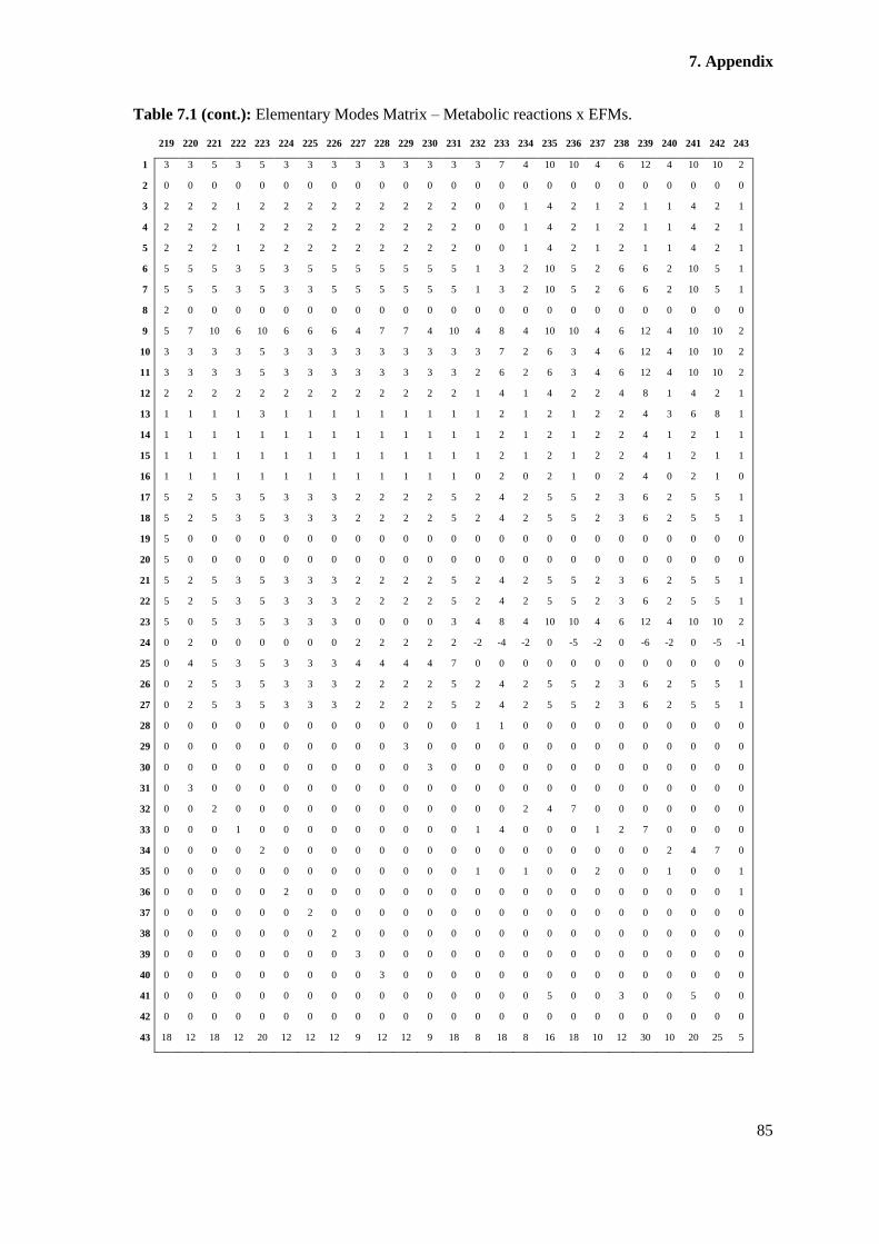
7. Appendix
85
Table 7.1 (cont.): Elementary Modes Matrix – Metabolic reactions x EFMs.
219 220 221 222 223 224 225 226 227 228 229 230 231 232 233 234 235 236 237 238 239 240 241 242 243
1 3 3 5 3 5 3 3 3 3 3 3 3 3 3 7 4 10 10 4 6 12 4 10 10 2
2 0 0 0 0 0 0 0 0 0 0 0 0 0 0 0 0 0 0 0 0 0 0 0 0 0
3 2 2 2 1 2 2 2 2 2 2 2 2 2 0 0 1 4 2 1 2 1 1 4 2 1
4 2 2 2 1 2 2 2 2 2 2 2 2 2 0 0 1 4 2 1 2 1 1 4 2 1
5 2 2 2 1 2 2 2 2 2 2 2 2 2 0 0 1 4 2 1 2 1 1 4 2 1
6 5 5 5 3 5 3 5 5 5 5 5 5 5 1 3 2 10 5 2 6 6 2 10 5 1
7 5 5 5 3 5 3 3 5 5 5 5 5 5 1 3 2 10 5 2 6 6 2 10 5 1
8 2 0 0 0 0 0 0 0 0 0 0 0 0 0 0 0 0 0 0 0 0 0 0 0 0
9 5 7 10 6 10 6 6 6 4 7 7 4 10 4 8 4 10 10 4 6 12 4 10 10 2
10 3 3 3 3 5 3 3 3 3 3 3 3 3 3 7 2 6 3 4 6 12 4 10 10 2
11 3 3 3 3 5 3 3 3 3 3 3 3 3 2 6 2 6 3 4 6 12 4 10 10 2
12 2 2 2 2 2 2 2 2 2 2 2 2 2 1 4 1 4 2 2 4 8 1 4 2 1
13 1 1 1 1 3 1 1 1 1 1 1 1 1 1 2 1 2 1 2 2 4 3 6 8 1
14 1 1 1 1 1 1 1 1 1 1 1 1 1 1 2 1 2 1 2 2 4 1 2 1 1
15 1 1 1 1 1 1 1 1 1 1 1 1 1 1 2 1 2 1 2 2 4 1 2 1 1
16 1 1 1 1 1 1 1 1 1 1 1 1 1 0 2 0 2 1 0 2 4 0 2 1 0
17 5 2 5 3 5 3 3 3 2 2 2 2 5 2 4 2 5 5 2 3 6 2 5 5 1
18 5 2 5 3 5 3 3 3 2 2 2 2 5 2 4 2 5 5 2 3 6 2 5 5 1
19 5 0 0 0 0 0 0 0 0 0 0 0 0 0 0 0 0 0 0 0 0 0 0 0 0
20 5 0 0 0 0 0 0 0 0 0 0 0 0 0 0 0 0 0 0 0 0 0 0 0 0
21 5 2 5 3 5 3 3 3 2 2 2 2 5 2 4 2 5 5 2 3 6 2 5 5 1
22 5 2 5 3 5 3 3 3 2 2 2 2 5 2 4 2 5 5 2 3 6 2 5 5 1
23 5 0 5 3 5 3 3 3 0 0 0 0 3 4 8 4 10 10 4 6 12 4 10 10 2
24 0 2 0 0 0 0 0 0 2 2 2 2 2 -2 -4 -2 0 -5 -2 0 -6 -2 0 -5 -1
25 0 4 5 3 5 3 3 3 4 4 4 4 7 0 0 0 0 0 0 0 0 0 0 0 0
26 0 2 5 3 5 3 3 3 2 2 2 2 5 2 4 2 5 5 2 3 6 2 5 5 1
27 0 2 5 3 5 3 3 3 2 2 2 2 5 2 4 2 5 5 2 3 6 2 5 5 1
28 0 0 0 0 0 0 0 0 0 0 0 0 0 1 1 0 0 0 0 0 0 0 0 0 0
29 0 0 0 0 0 0 0 0 0 0 3 0 0 0 0 0 0 0 0 0 0 0 0 0 0
30 0 0 0 0 0 0 0 0 0 0 0 3 0 0 0 0 0 0 0 0 0 0 0 0 0
31 0 3 0 0 0 0 0 0 0 0 0 0 0 0 0 0 0 0 0 0 0 0 0 0 0
32 0 0 2 0 0 0 0 0 0 0 0 0 0 0 0 2 4 7 0 0 0 0 0 0 0
33 0 0 0 1 0 0 0 0 0 0 0 0 0 1 4 0 0 0 1 2 7 0 0 0 0
34 0 0 0 0 2 0 0 0 0 0 0 0 0 0 0 0 0 0 0 0 0 2 4 7 0
35 0 0 0 0 0 0 0 0 0 0 0 0 0 1 0 1 0 0 2 0 0 1 0 0 1
36 0 0 0 0 0 2 0 0 0 0 0 0 0 0 0 0 0 0 0 0 0 0 0 0 1
37 0 0 0 0 0 0 2 0 0 0 0 0 0 0 0 0 0 0 0 0 0 0 0 0 0
38 0 0 0 0 0 0 0 2 0 0 0 0 0 0 0 0 0 0 0 0 0 0 0 0 0
39 0 0 0 0 0 0 0 0 3 0 0 0 0 0 0 0 0 0 0 0 0 0 0 0 0
40 0 0 0 0 0 0 0 0 0 3 0 0 0 0 0 0 0 0 0 0 0 0 0 0 0
41 0 0 0 0 0 0 0 0 0 0 0 0 0 0 0 0 5 0 0 3 0 0 5 0 0
42 0 0 0 0 0 0 0 0 0 0 0 0 0 0 0 0 0 0 0 0 0 0 0 0 0
43 18 12 18 12 20 12 12 12 9 12 12 9 18 8 18 8 16 18 10 12 30 10 20 25 5
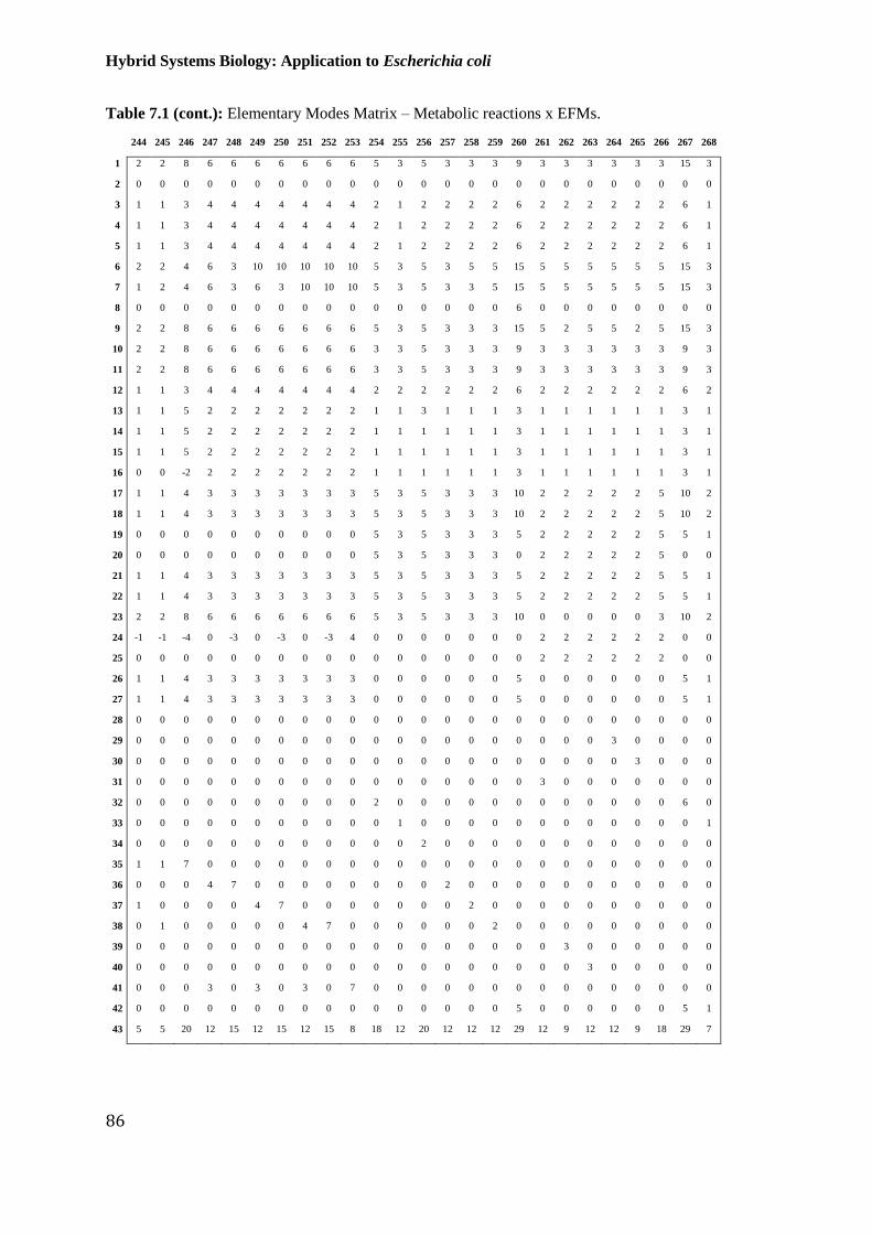
Hybrid Systems Biology: Application to Escherichia coli
86
Table 7.1 (cont.): Elementary Modes Matrix – Metabolic reactions x EFMs.
244 245 246 247 248 249 250 251 252 253 254 255 256 257 258 259 260 261 262 263 264 265 266 267 268
1 2 2 8 6 6 6 6 6 6 6 5 3 5 3 3 3 9 3 3 3 3 3 3 15 3
2 0 0 0 0 0 0 0 0 0 0 0 0 0 0 0 0 0 0 0 0 0 0 0 0 0
3 1 1 3 4 4 4 4 4 4 4 2 1 2 2 2 2 6 2 2 2 2 2 2 6 1
4 1 1 3 4 4 4 4 4 4 4 2 1 2 2 2 2 6 2 2 2 2 2 2 6 1
5 1 1 3 4 4 4 4 4 4 4 2 1 2 2 2 2 6 2 2 2 2 2 2 6 1
6 2 2 4 6 3 10 10 10 10 10 5 3 5 3 5 5 15 5 5 5 5 5 5 15 3
7 1 2 4 6 3 6 3 10 10 10 5 3 5 3 3 5 15 5 5 5 5 5 5 15 3
8 0 0 0 0 0 0 0 0 0 0 0 0 0 0 0 0 6 0 0 0 0 0 0 0 0
9 2 2 8 6 6 6 6 6 6 6 5 3 5 3 3 3 15 5 2 5 5 2 5 15 3
10 2 2 8 6 6 6 6 6 6 6 3 3 5 3 3 3 9 3 3 3 3 3 3 9 3
11 2 2 8 6 6 6 6 6 6 6 3 3 5 3 3 3 9 3 3 3 3 3 3 9 3
12 1 1 3 4 4 4 4 4 4 4 2 2 2 2 2 2 6 2 2 2 2 2 2 6 2
13 1 1 5 2 2 2 2 2 2 2 1 1 3 1 1 1 3 1 1 1 1 1 1 3 1
14 1 1 5 2 2 2 2 2 2 2 1 1 1 1 1 1 3 1 1 1 1 1 1 3 1
15 1 1 5 2 2 2 2 2 2 2 1 1 1 1 1 1 3 1 1 1 1 1 1 3 1
16 0 0 -2 2 2 2 2 2 2 2 1 1 1 1 1 1 3 1 1 1 1 1 1 3 1
17 1 1 4 3 3 3 3 3 3 3 5 3 5 3 3 3 10 2 2 2 2 2 5 10 2
18 1 1 4 3 3 3 3 3 3 3 5 3 5 3 3 3 10 2 2 2 2 2 5 10 2
19 0 0 0 0 0 0 0 0 0 0 5 3 5 3 3 3 5 2 2 2 2 2 5 5 1
20 0 0 0 0 0 0 0 0 0 0 5 3 5 3 3 3 0 2 2 2 2 2 5 0 0
21 1 1 4 3 3 3 3 3 3 3 5 3 5 3 3 3 5 2 2 2 2 2 5 5 1
22 1 1 4 3 3 3 3 3 3 3 5 3 5 3 3 3 5 2 2 2 2 2 5 5 1
23 2 2 8 6 6 6 6 6 6 6 5 3 5 3 3 3 10 0 0 0 0 0 3 10 2
24 -1 -1 -4 0 -3 0 -3 0 -3 4 0 0 0 0 0 0 0 2 2 2 2 2 2 0 0
25 0 0 0 0 0 0 0 0 0 0 0 0 0 0 0 0 0 2 2 2 2 2 2 0 0
26 1 1 4 3 3 3 3 3 3 3 0 0 0 0 0 0 5 0 0 0 0 0 0 5 1
27 1 1 4 3 3 3 3 3 3 3 0 0 0 0 0 0 5 0 0 0 0 0 0 5 1
28 0 0 0 0 0 0 0 0 0 0 0 0 0 0 0 0 0 0 0 0 0 0 0 0 0
29 0 0 0 0 0 0 0 0 0 0 0 0 0 0 0 0 0 0 0 0 3 0 0 0 0
30 0 0 0 0 0 0 0 0 0 0 0 0 0 0 0 0 0 0 0 0 0 3 0 0 0
31 0 0 0 0 0 0 0 0 0 0 0 0 0 0 0 0 0 3 0 0 0 0 0 0 0
32 0 0 0 0 0 0 0 0 0 0 2 0 0 0 0 0 0 0 0 0 0 0 0 6 0
33 0 0 0 0 0 0 0 0 0 0 0 1 0 0 0 0 0 0 0 0 0 0 0 0 1
34 0 0 0 0 0 0 0 0 0 0 0 0 2 0 0 0 0 0 0 0 0 0 0 0 0
35 1 1 7 0 0 0 0 0 0 0 0 0 0 0 0 0 0 0 0 0 0 0 0 0 0
36 0 0 0 4 7 0 0 0 0 0 0 0 0 2 0 0 0 0 0 0 0 0 0 0 0
37 1 0 0 0 0 4 7 0 0 0 0 0 0 0 2 0 0 0 0 0 0 0 0 0 0
38 0 1 0 0 0 0 0 4 7 0 0 0 0 0 0 2 0 0 0 0 0 0 0 0 0
39 0 0 0 0 0 0 0 0 0 0 0 0 0 0 0 0 0 0 3 0 0 0 0 0 0
40 0 0 0 0 0 0 0 0 0 0 0 0 0 0 0 0 0 0 0 3 0 0 0 0 0
41 0 0 0 3 0 3 0 3 0 7 0 0 0 0 0 0 0 0 0 0 0 0 0 0 0
42 0 0 0 0 0 0 0 0 0 0 0 0 0 0 0 0 5 0 0 0 0 0 0 5 1
43 5 5 20 12 15 12 15 12 15 8 18 12 20 12 12 12 29 12 9 12 12 9 18 29 7
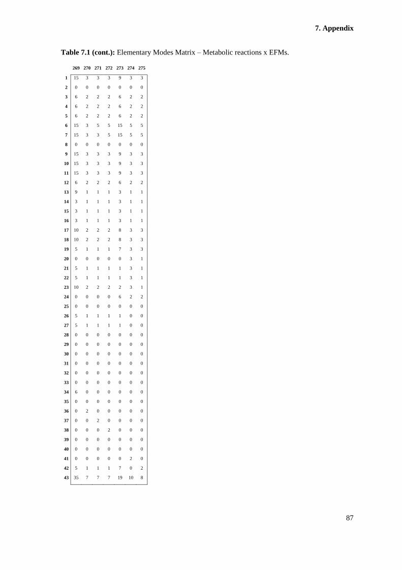
7. Appendix
87
Table 7.1 (cont.): Elementary Modes Matrix – Metabolic reactions x EFMs.
269 270 271 272 273 274 275
1 15 3 3 3 9 3 3
2 0 0 0 0 0 0 0
3 6 2 2 2 6 2 2
4 6 2 2 2 6 2 2
5 6 2 2 2 6 2 2
6 15 3 5 5 15 5 5
7 15 3 3 5 15 5 5
8 0 0 0 0 0 0 0
9 15 3 3 3 9 3 3
10 15 3 3 3 9 3 3
11 15 3 3 3 9 3 3
12 6 2 2 2 6 2 2
13 9 1 1 1 3 1 1
14 3 1 1 1 3 1 1
15 3 1 1 1 3 1 1
16 3 1 1 1 3 1 1
17 10 2 2 2 8 3 3
18 10 2 2 2 8 3 3
19 5 1 1 1 7 3 3
20 0 0 0 0 0 3 1
21 5 1 1 1 1 3 1
22 5 1 1 1 1 3 1
23 10 2 2 2 2 3 1
24 0 0 0 0 6 2 2
25 0 0 0 0 0 0 0
26 5 1 1 1 1 0 0
27 5 1 1 1 1 0 0
28 0 0 0 0 0 0 0
29 0 0 0 0 0 0 0
30 0 0 0 0 0 0 0
31 0 0 0 0 0 0 0
32 0 0 0 0 0 0 0
33 0 0 0 0 0 0 0
34 6 0 0 0 0 0 0
35 0 0 0 0 0 0 0
36 0 2 0 0 0 0 0
37 0 0 2 0 0 0 0
38 0 0 0 2 0 0 0
39 0 0 0 0 0 0 0
40 0 0 0 0 0 0 0
41 0 0 0 0 0 2 0
42 5 1 1 1 7 0 2
43 35 7 7 7 19 10 8
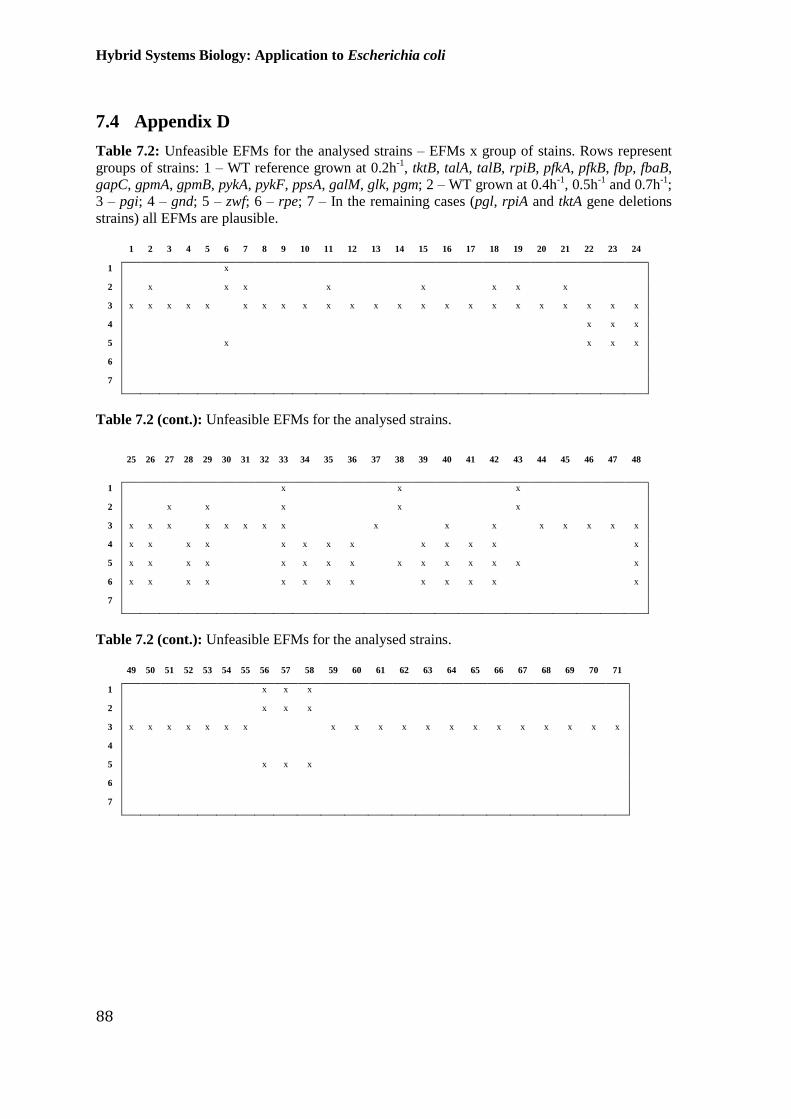
Hybrid Systems Biology: Application to Escherichia coli
88
7.4 Appendix D
Table 7.2: Unfeasible EFMs for the analysed strains – EFMs x group of stains. Rows represent
groups of strains: 1 – WT reference grown at 0.2h-1
, tktB, talA, talB, rpiB, pfkA, pfkB, fbp, fbaB,
gapC, gpmA, gpmB, pykA, pykF, ppsA, galM, glk, pgm; 2 – WT grown at 0.4h-1
, 0.5h-1
and 0.7h-1
;
3 – pgi; 4 – gnd; 5 – zwf; 6 – rpe; 7 – In the remaining cases (pgl, rpiA and tktA gene deletions
strains) all EFMs are plausible.
1 2 3 4 5 6 7 8 9 10 11 12 13 14 15 16 17 18 19 20 21 22 23 24
1
x
2
x
x x
x
x
x x
x
3 x x x x x
x x x x x x x x x x x x x x x x x x
4
x x x
5
x
x x x
6
7
Table 7.2 (cont.): Unfeasible EFMs for the analysed strains.
25 26 27 28 29 30 31 32 33 34 35 36 37 38 39 40 41 42 43 44 45 46 47 48
1
x
x
x
2
x
x
x
x
x
3 x x x
x x x x x
x
x
x
x x x x x
4 x x
x x
x x x x
x x x x
x
5 x x
x x
x x x x
x x x x x x
x
6 x x
x x
x x x x
x x x x
x
7
Table 7.2 (cont.): Unfeasible EFMs for the analysed strains.
49 50 51 52 53 54 55 56 57 58 59 60 61 62 63 64 65 66 67 68 69 70 71
1
x x x
2
x x x
3 x x x x x x x
x x x x x x x x x x x x x
4
5
x x x
6
7

7. Appendix
89
Table 7.2 (cont.): Unfeasible EFMs for the analysed strains.
72 73 74 75 76 77 78 79 80 81 82 83 84 85 86 87 88 89 90 91 92 93 94
1
x
2
x
x x x x x x x
3 x x x x x x x x x x x x x x x x x x x x x x
4
x
x x x x x x x x
x x
5
x
x x x x x x x x
x x x
6
x
x
x x x
7
Table 7.2 (cont.): Unfeasible EFMs for the analysed strains.
95 96 97 98 99 100 101 102 103 104 105 106 107 108 109 110 111 112 113 114 115 116 117 118
1
x
x x x x x x
x x x
2
x
x x x x x x
x x x x x
3 x x x x
x
x
x x x x x x x x x
4 x x x x
x x x x
5 x x x x x
x x x x x x
x x x x x
6
x x
7
Table 7.2 (cont.): Unfeasible EFMs for the analysed strains.
119 120 121 122 123 124 125 126 127 128 129 130 131 132 133 134 135 136 137 138 139 140 141 142 143 144
1
2 x x x x x x x x x x
x
x x x x x x x
3 x x x x x x x x x x x x x x x x x x x x x x x x x x
4 x x x x x x x x x x x x x x
5 x x x x x x x x x x x x x x
6 x x x
x
x x x x x x
7
Table 7.2 (cont.): Unfeasible EFMs for the analysed strains.
145 146 147 148 149 150 151 152 153 154 155 156 157 158 159 160 161 162 163 164 165 166 167 168 169
1
2 x x x x x x x x x x x x x x x x x x x x
3 x x x x x x x x x x x x x x x x x
4
x x x x x x x x x x x x x x
5
x x x x x x x x x x x x x x
6
x x x x x x x x
7

Hybrid Systems Biology: Application to Escherichia coli
90
Table 7.2 (cont.): Unfeasible EFMs for the analysed strains.
170 171 172 173 174 175 176 177 178 179 180 181 182 183 184 185 186 187 188 189 190 191 192 193
1
2
3
4 x x x x x x x x x x x x x x x x x x x x x x x x
5 x x x x x x x x x x x x x x x x x x x x x x x x
6 x x x x x x x x x x x x x x x x x x x x x x x x
7
Table 7.2 (cont.): Unfeasible EFMs for the analysed strains.
194 195 196 197 198 199 200 201 202 203 204 205 206 207 208 209 210 211 212 213 214 215 216 217
1
2
x x x
3
4 x x x x x x x x x x x x x x x x x x x x x x x x
5 x x x x x x x x x x x x x x x x x x x x x x x x
6 x x x x x x x x x x x x x x x x x x x x x x x x
7
Table 7.2 (cont.): Unfeasible EFMs for the analysed strains.
218 219 220 221 222 223 224 225 226 227 228 229 230 231 232 233 234 235 236 237 238 239 240 241 242
1
x x
2 x
x x x x x x x x x x x x x x x x x x x x x x x
3
4 x x x x x x x x x x x x x x x x x x x x x x x x x
5 x x x x x x x x x x x x x x x x x x x x x x x x x
6 x x x x x x x x x x x x x x x x x x x x x x x x x
7
Table 7.2 (cont.): Unfeasible EFMs for the analysed strains.
243 244 245 246 247 248 249 250 251 252 253 254 255 256 257 258 259 260 261 262 263
1
2 x x x x x x x x x x x
x
3
4 x x x x x x x x x x x x x x x x x x x x x
5 x x x x x x x x x x x x x x x x x x x x x
6 x x x x x x x x x x x x x x x x x x x x x
7

7. Appendix
91
Table 7.2 (cont.): Unfeasible EFMs for the analysed strains.
264 265 266 267 268 269 270 271 272 273 274 275
1
2
x x x x x x x
3
4 x x x x x x x x x x x x
5 x x x x x x x x x x x x
6 x x x x x x x x x x x x
7
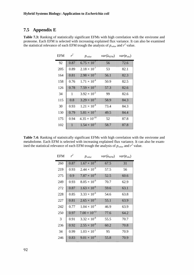
Hybrid Systems Biology: Application to Escherichia coli
92
7.5 Appendix E
Table 7.3: Ranking of statistically significant EFMs with high correlation with the envirome and
proteome. Each EFM is selected with increasing explained flux variance. It can also be examined
the statistical relevance of each EFM trough the analysis of pvalue and r2 value.
EFM r2 pvalue var(λEFM) var(robs)
92 0.87 6.75 × 10⁻⁷
56 72.6
205 0.89 2.18 × 10⁻⁷
53 82.1
164 0.81 2.98 × 10⁻⁵
56.1 82.3
158 0.76 1.71 × 10⁻⁴
50.9 82.5
126 0.78 7.59 × 10⁻⁵
57.3 82.6
34 1 3.92 × 10⁻²
99 82.6
115 0.8 3.29 × 10⁻⁵
58.9 84.3
30 0.93 1.21 × 10⁻⁸
73.4 84.3
130 0.79 5.81 × 10⁻⁵
49.5 84.4
175 0.94 4.35 × 10⁻¹⁰
52 87.8
102 1 1.54 × 10⁻²
58.7 87.8
Table 7.4: Ranking of statistically significant EFMs with high correlation with the envirome and
metabolome. Each EFM is selected with increasing explained flux variance. It can also be exam-
ined the statistical relevance of each EFM trough the analysis of pvalue and r2 value.
EFM r2 pvalue var(λEFM) var(robs)
260 0.87 1.67 × 10⁻⁶
67.5 31
219 0.93 2.44 × 10⁻⁹
57.5 56
275 0.9 7.87 × 10⁻⁸
52.5 60.6
249 0.93 8.05 × 10⁻⁹
70.7 62.9
272 0.87 1.63 × 10⁻⁶
59.6 63.1
228 0.85 3.33 × 10⁻⁶
54.6 63.8
227 0.81 2.65 × 10⁻⁵
55.1 63.9
242 0.77 1.04 × 10⁻⁴
46.9 63.9
250 0.97 7.00 × 10⁻¹²
77.6 64.2
3 0.91 3.32 × 10⁻⁸
55.5 70.7
236 0.92 2.55 × 10⁻⁸
60.2 70.8
34 0.99 1.03 × 10⁻¹
95 70.9
246 0.83 9.01 × 10⁻⁶
55.8 70.9
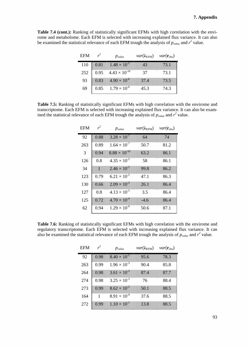
7. Appendix
93
Table 7.4 (cont.): Ranking of statistically significant EFMs with high correlation with the envi-
rome and metabolome. Each EFM is selected with increasing explained flux variance. It can also
be examined the statistical relevance of each EFM trough the analysis of pvalue and r2 value.
EFM r2 pvalue var(λEFM) var(robs)
110 0.81 1.48 × 10⁻⁵
43 73.1
252 0.95 4.43 × 10⁻¹⁰
37 73.1
93 0.83 4.90 × 10⁻⁶
37.4 73.5
69 0.85 1.79 × 10⁻⁶
45.3 74.3
Table 7.5: Ranking of statistically significant EFMs with high correlation with the envirome and
transcriptome. Each EFM is selected with increasing explained flux variance. It can also be exam-
ined the statistical relevance of each EFM trough the analysis of pvalue and r2 value.
EFM r2 pvalue var(λEFM) var(robs)
92 0.88 3.28 × 10⁻⁷
64 74
263 0.89 1.64 × 10⁻⁷
50.7 81.2
3 0.94 8.88 × 10⁻¹⁰
63.2 86.1
126 0.8 4.35 × 10⁻⁵
58 86.1
34 1 2.46 × 10⁻²
99.8 86.2
123 0.79 6.21 × 10⁻⁵
47.1 86.3
130 0.66 2.09 × 10⁻³
26.1 86.4
127 0.8 4.13 × 10⁻⁵
3.5 86.4
125 0.72 4.70 × 10⁻⁴
-4.6 86.4
62 0.94 1.29 × 10⁻⁹
50.6 87.1
Table 7.6: Ranking of statistically significant EFMs with high correlation with the envirome and
regulatory transcriptome. Each EFM is selected with increasing explained flux variance. It can
also be examined the statistical relevance of each EFM trough the analysis of pvalue and r2 value.
EFM r2 pvalue var(λEFM) var(robs)
92 0.98 8.40 × 10⁻⁵
95.6 78.3
263 0.99 1.96 × 10⁻³
90.4 85.8
264 0.98 3.61 × 10⁻³
87.4 87.7
274 0.98 3.25 × 10⁻³
76 88.4
273 0.99 8.62 × 10⁻²
50.1 88.5
164 1 8.91 × 10⁻⁴
37.6 88.5
272 0.99 1.10 × 10⁻¹
13.8 88.5

Hybrid Systems Biology: Application to Escherichia coli
94
Table 7.6 (cont.): Ranking of statistically significant EFMs with high correlation with the envi-
rome and regulatory transcriptome. Each EFM is selected with increasing explained flux variance.
It can also be examined the statistical relevance of each EFM trough the analysis of pvalue and r2
value.
EFM r2 pvalue var(λEFM) var(robs)
262 0.96 8.65 × 10⁻³
68 88.5
162 1 1.09 × 10⁻³
50.3 88.5
275 0.99 4.72 × 10⁻⁴
53.5 88.6
227 1 2.80 × 10⁻²
32.4 88.6
126 1 9.77 × 10⁻³
70.5 88.6
124 1 7.18 × 10⁻⁴
90.8 88.6
258 0.98 3.43 × 10⁻³
44.7 88.7
211 1 1.03 × 10⁻⁴
92 88.8
158 1 2.40 × 10⁻⁴
46.6 88.8
157 1 1.05 × 10⁻³
51.8 88.8
122 1 1.61 × 10⁻³
74.3 88.9
154 0.98 3.30 × 10⁻³
68.4 89.1
3 0.95 1.21 × 10⁻³
79.9 89.7
Table 7.7: Ranking of statistically significant EFMs with high correlation with the proteome and
metabolome. Each EFM is selected with increasing explained flux variance. It can also be exam-
ined the statistical relevance of each EFM trough the analysis of pvalue and r2 value.
EFM r2 pvalue var(λEFM) var(robs)
260 0.9 1.86 × 10⁻⁷
66.6 31
219 0.9 7.60 × 10⁻⁸
57.2 55.8
263 0.88 2.56 × 10⁻⁷
47.3 61
249 0.86 2.73 × 10⁻⁶
60.5 61.6
241 0.86 2.03 × 10⁻⁶
62.2 61.7
228 0.96 7.91 × 10⁻¹¹
55.8 62.5
235 0.96 1.66 × 10⁻¹⁰
45.9 62.5
242 0.92 2.49 × 10⁻⁸
39.9 62.5
34 0.99 8.21 × 10⁻²
97.2 62.6
244 0.9 1.17 × 10⁻⁷
42.2 62.6
3 0.89 1.02 × 10⁻⁷
53.7 68.6
79 0.88 3.22 × 10⁻⁷
19.4 68.9
71 0.89 1.50 × 10⁻⁷
49.7 71

7. Appendix
95
Table 7.8: Ranking of statistically significant EFMs with high correlation with the proteome and
Transcriptome. Each EFM is selected with increasing explained flux variance. It can also be ex-
amined the statistical relevance of each EFM trough the analysis of pvalue and r2 value.
EFM r2 pvalue var(λEFM) var(robs)
92 0.89 1.04 × 10⁻⁷
54.1 72.2
263 0.95 1.13 × 10⁻¹⁰
51.8 80
164 0.86 1.86 × 10⁻⁶
37.9 80.2
30 0.82 1.77 × 10⁻⁵
50.4 80.3
228 0.85 3.18 × 10⁻⁶
39.7 80.6
3 0.96 2.47 × 10⁻¹¹
54.3 85.4
126 0.81 2.74 × 10⁻⁵
51.7 85.5
124 0.96 1.24 × 10⁻¹⁰
39.1 85.5
34 1 1.21 × 10⁻²
100 85.5
121 0.79 5.55 × 10⁻⁵
49.1 85.5
119 0.76 1.73 × 10⁻⁴
46.2 85.7
130 0.85 4.24 × 10⁻⁶
38.2 85.7
120 0.85 3.19 × 10⁻⁶
43.6 85.8
115 0.87 1.75 × 10⁻⁶
54.1 86.9
244 0.96 3.57 × 10⁻¹¹
50.7 87.4
127 0.96 1.26 × 10⁻¹⁰
66.5 87.5
157 0.93 1.34 × 10⁻⁸
37.8 87.6
71 0.97 6.12 × 10⁻¹²
49.7 89.1
Table 7.9: Ranking of statistically significant EFMs with high correlation with the proteome and
regulatory transcriptome. Each EFM is selected with increasing explained flux variance. It can
also be examined the statistical relevance of each EFM trough the analysis of pvalue and r2 value.
EFM r2 pvalue var(λEFM) var(robs)
92 0.97 1.88 × 10⁻⁴
94.1 78
263 0.98 3.86 × 10⁻³
88.8 85.5
264 0.98 4.33 × 10⁻³
87.7 87.5
274 0.99 4.67 × 10⁻⁴
81.5 88.2
273 1 8.14 × 10⁻³
50.7 88.3
164 1 4.49 × 10⁻⁴
43.7 88.3
260 1 1.03 × 10⁻³
13.5 88.4
262 0.91 3.27 × 10⁻²
64.5 88.4

Hybrid Systems Biology: Application to Escherichia coli
96
Table 7.9 (cont.): Ranking of statistically significant EFMs with high correlation with the prote-
ome and regulatory transcriptome. Each EFM is selected with increasing explained flux variance.
It can also be examined the statistical relevance of each EFM trough the analysis of pvalue and r2
value.
EFM r2 pvalue var(λEFM) var(robs)
162 1 9.20 × 10⁻⁴
75.3 88.4
275 0.98 3.56 × 10⁻³
49 88.5
227 1 4.35 × 10⁻⁴
38.3 88.5
124 1 1.08 × 10⁻³
95.1 88.5
158 1 1.34 × 10⁻³
49 88.6
115 1 6.77 × 10⁻⁴
43.1 88.8
253 1 3.11 × 10⁻³
77.5 88.8
126 1 1.39 × 10⁻³
99 88.8
211 1 1.25 × 10⁻⁵
95.3 89
157 1 8.43 × 10⁻⁵
65.2 89
122 1 1.46 × 10⁻⁴
90.6 89
154 1 1.53 × 10⁻⁴
83.6 89.3
Table 7.10: Ranking of statistically significant EFMs with high correlation with the metabolome
and transcriptome. Each EFM is selected with increasing explained flux variance. It can also be
examined the statistical relevance of each EFM trough the analysis of pvalue and r2 value.
EFM r2 pvalue var(λEFM) var(robs)
92 0.93 3.71 × 10⁻⁹
59.3 73.1
263 0.92 1.13 × 10⁻⁸
51.5 80.5
3 0.95 2.90 × 10⁻¹⁰
53.4 85
116 0.8 3.56 × 10⁻⁵
62.6 85.8
30 0.77 1.07 × 10⁻⁴
56.9 85.8
126 0.79 6.08 × 10⁻⁵
50.1 86.1
123 0.79 6.65 × 10⁻⁵
44.9 86.1
125 0.89 3.68 × 10⁻⁷
57.5 86.2
102 1 6.12 × 10⁻²
72.2 86.2
71 0.95 1.87 × 10⁻¹⁰
47.4 87.7
120 0.87 1.06 × 10⁻⁶
55.9 87.8
121 0.87 1.30 × 10⁻⁶
61 87.9
7. Appendix
97
Table 7.11: Ranking of statistically significant EFMs with high correlation with the metabolome
and regulatory transcriptome. Each EFM is selected with increasing explained flux variance. It
can also be examined the statistical relevance of each EFM trough the analysis of pvalue and r2 val-
ue.
EFM r2 pvalue var(λEFM) var(robs)
92 1 3.35 × 10⁻⁷
99.3 79.1
263 1 1.51 × 10⁻⁵
95.8 86.3
264 1 7.50 × 10⁻⁶
97.7 88.2
274 1 1.82 × 10⁻⁵
63.9 88.8
164 1 6.66 × 10⁻⁵
59.6 88.8
262 1 3.47 × 10⁻⁵
36.5 88.9
162 1 1.08 × 10⁻³
61.5 88.9
158 1 8.72 × 10⁻⁴
52.5 88.9
126 1 2.29 × 10⁻²
86.5 89
211 1 1.85 × 10⁻⁶
81.6 89.1
157 1 1.61 × 10⁻³
56.6 89.1
154 1 1.33 × 10⁻⁵
92.5 89.4
3 0.97 3.55 × 10⁻⁴
83.7 90
155 1 6.49 × 10⁻⁵
81.4 90
153 1 8.31 × 10⁻⁵
80 90.1
151 0.99 5.78 × 10⁻⁴
78.6 90.1
202 0.99 6.34 × 10⁻⁴
81.9 90.1
134 0.99 1.02 × 10⁻⁵
93.9 92
273 1 1.91 × 10⁻³
68 92
275 1 1.01 × 10⁻⁵
96.6 92.1
Table 7.12: Ranking of statistically significant EFMs with high correlation with the transcriptome
and regulatory transcriptome. Each EFM is selected with increasing explained flux variance. It
can also be examined the statistical relevance of each EFM trough the analysis of pvalue and r2 val-
ue.
EFM r2 pvalue var(λEFM) var(robs)
92 0.97 4.14 × 10⁻⁴
91.8 77.5
263 0.98 2.47 × 10⁻³
88.7 85.3
264 0.99 1.20 × 10⁻³
86.7 87.4
271 1 2.72 × 10⁻³
59.4 87.7
274 0.99 4.96 × 10⁻⁴
83.3 88.2

Hybrid Systems Biology: Application to Escherichia coli
98
Table 7.12 (cont.): Ranking of statistically significant EFMs with high correlation with the tran-
scriptome and regulatory transcriptome. Each EFM is selected with increasing explained flux var-
iance. It can also be examined the statistical relevance of each EFM trough the analysis of pvalue
and r2 value.
EFM r2 pvalue var(λEFM) var(robs)
164 1 2.03 × 10⁻⁴
40.2 88.2
269 0.99 9.10 × 10⁻²
34.9 88.3
260 1 3.13 × 10⁻²
20.1 88.4
275 0.98 2.30 × 10⁻³
88 88.4
273 1 6.00 × 10⁻²
36.2 88.4
272 1 5.14 × 10⁻²
30.9 88.4
253 1 1.61 × 10⁻²
75 88.5
162 1 4.87 × 10⁻⁴
58.8 88.5
262 0.99 1.83 × 10⁻³
75.9 88.5
227 0.99 9.95 × 10⁻²
66.2 88.5
258 0.98 2.61 × 10⁻³
79.3 88.6
247 1 4.89 × 10⁻²
21.8 88.6
124 1 1.97 × 10⁻³
98.8 88.6
158 1 1.23 × 10⁻³
73.2 88.7
211 1 7.03 × 10⁻⁵
98.3 88.8
Table 7.13: Ranking of statistically significant EFMs with high correlation with the envirome,
proteome and metabolome. Each EFM is selected with increasing explained flux variance. Statis-
tical relevance of each EFM can also be examined (pvalue and r2 value).
EFM r2 pvalue var(λEFM) var(robs)
260 0.9 1.11 × 10⁻⁷
67.3 31
219 0.93 1.67 × 10⁻⁹
59.8 56.5
262 0.92 7.83 × 10⁻⁹
48.3 60.9
249 0.86 3.08 × 10⁻⁶
58.4 61.5
241 0.84 7.37 × 10⁻⁶
62.7 61.5
227 0.92 2.42 × 10⁻⁸
53.9 62.2
236 0.94 1.39 × 10⁻⁹
68.6 62.3
233 0.99 1.00 × 10⁻¹
69.4 62.3
231 0.86 2.31 × 10⁻⁶
46.7 62.7
253 0.96 6.32 × 10⁻¹¹
54.2 63
3 0.95 3.07 × 10⁻¹⁰
50 67.3

7. Appendix
99
Table 7.13 (cont.): Ranking of statistically significant EFMs with high correlation with the envi-
rome, proteome and metabolome. Each EFM is selected with increasing explained flux variance.
It can also be examined the statistical relevance of each EFM trough the analysis of pvalue and r2
value.
EFM r2 pvalue var(λEFM) var(robs)
228 0.87 1.70 × 10⁻⁶
47.8 67.4
250 0.98 4.56 × 10⁻¹³
23.9 67.4
94 0.85 2.28 × 10⁻⁶
39.3 67.7
70 0.92 9.88 × 10⁻⁹
50.9 70.8
34 0.99 8.37 × 10⁻²
97.2 70.9
246 0.93 1.31 × 10⁻⁸
55.9 71.1
106 1 5.37 × 10⁻²
53.9 71.7
Table 7.14: Ranking of statistically significant EFMs with high correlation with the envirome,
proteome and transcriptome. Each EFM is selected with increasing explained flux variance. It can
also be examined the statistical relevance of each EFM trough the analysis of pvalue and r2 value.
EFM r2 pvalue var(λEFM) var(robs)
92 0.9 8.68 × 10⁻⁸
55 72.4
263 0.96 6.64 × 10⁻¹²
55.8 80.4
164 0.89 4.21 × 10⁻⁷
40.5 80.6
30 0.85 4.45 × 10⁻⁶
48.2 80.7
3 0.96 1.71 × 10⁻¹¹
56.1 85.3
126 0.84 6.93 × 10⁻⁶
59.5 85.4
34 1 2.59 × 10⁻²
99.8 85.4
121 0.83 9.72 × 10⁻⁶
52.3 85.4
130 0.84 6.45 × 10⁻⁶
43.4 85.6
123 0.9 1.91 × 10⁻⁷
46.6 85.6
127 0.88 7.48 × 10⁻⁷
45.2 85.6
125 0.78 9.22 × 10⁻⁵
16.1 85.6
115 0.87 1.17 × 10⁻⁶
56.8 86.9
244 0.96 1.03 × 10⁻¹⁰
53.9 87.3
119 0.99 1.78 × 10⁻¹⁴
58.4 87.4
120 0.96 4.45 × 10⁻¹¹
29.7 87.4
128 0.9 1.03 × 10⁻⁷
31.5 87.4
71 0.97 3.01 × 10⁻¹²
50.6 88.9

Hybrid Systems Biology: Application to Escherichia coli
100
Table 7.15: Ranking of statistically significant EFMs with high correlation with the envirome,
proteome and regulatory transcriptome. Each EFM is selected with increasing explained flux var-
iance. It can also be examined the statistical relevance of each EFM trough the analysis of pvalue
and r2 value.
EFM r2 pvalue var(λEFM) var(robs)
92 0.98 1.29 × 10⁻⁴
94.9 78.2
263 0.98 2.46 × 10⁻³
90.4 85.7
264 0.98 2.72 × 10⁻³
89.4 87.6
274 1 8.99 × 10⁻⁵
79.7 88.3
273 1 8.68 × 10⁻³
46.1 88.4
164 1 4.53 × 10⁻⁴
42.6 88.4
262 0.97 5.73 × 10⁻³
73.3 88.5
162 1 6.01 × 10⁻⁴
64.1 88.5
275 0.99 1.18 × 10⁻³
50.5 88.5
124 1 4.96 × 10⁻⁴
92.4 88.5
229 1 5.87 × 10⁻³
75.7 88.7
253 1 3.72 × 10⁻³
52.4 88.7
126 1 7.07 × 10⁻⁴
69.1 88.8
121 1 3.77 × 10⁻³
41.6 88.8
132 1 1.47 × 10⁻⁵
98.3 88.9
246 1 4.65 × 10⁻³
73.2 88.9
160 1 4.04 × 10⁻⁴
46.4 88.9
163 1 3.62 × 10⁻³
53.2 89
216 1 1.99 × 10⁻³
12 89
244 1 4.63 × 10⁻⁴
72.4 89.1
Table 7.16: Ranking of statistically significant EFMs with high correlation with the envirome,
metabolome and transcriptome. Each EFM is selected with increasing explained flux variance. It
can also be examined the statistical relevance of each EFM trough the analysis of pvalue and r2 val-
ue.
EFM r2 pvalue var(λEFM) var(robs)
92 0.93 2.38 × 10⁻⁹
60.4 73.3
263 0.93 3.36 × 10⁻⁹
51.3 80.6
3 0.96 4.31 × 10⁻¹¹
53.7 85.2
119 0.8 4.63 × 10⁻⁵
63.2 85.4
126 0.89 3.04 × 10⁻⁷
76.2 85.5
7. Appendix
101
Table 7.16 (cont.): Ranking of statistically significant EFMs with high correlation with the envi-
rome, metabolome and transcriptome. Each EFM is selected with increasing explained flux vari-
ance. It can also be examined the statistical relevance of each EFM trough the analysis of pvalue
and r2 value.
EFM r2 pvalue var(λEFM) var(robs)
30 0.91 6.62 × 10⁻⁸
72.3 85.6
125 0.8 4.44 × 10⁻⁵
49.7 85.7
121 0.81 2.77 × 10⁻⁵
64 85.7
123 0.81 2.39 × 10⁻⁵
39.3 85.7
127 0.69 1.10 × 10⁻³
42.6 85.7
102 1 6.11 × 10⁻²
73.6 85.8
130 0.78 7.16 × 10⁻⁵
38.3 85.8
62 0.96 5.39 × 10⁻¹¹
49.6 86.5
13 0.81 1.39 × 10⁻⁵
35.2 86.7
Table 7.17: Ranking of statistically significant EFMs with high correlation with the envirome,
metabolome and regulatory transcriptome. Each EFM is selected with increasing explained flux
variance. It can also be examined the statistical relevance of each EFM trough the analysis of
pvalue and r2 value.
EFM r2 pvalue var(λEFM) var(robs)
92 1 4.54 × 10⁻⁷
99.3 79.1
263 1 1.45 × 10⁻⁵
96 86.3
264 1 8.96 × 10⁻⁶
97.9 88.2
274 1 2.35 × 10⁻⁵
63.8 88.8
164 1 1.05 × 10⁻⁴
60.1 88.8
162 1 1.56 × 10⁻³
60 88.8
262 1 6.67 × 10⁻⁵
34.4 88.9
158 1 9.12 × 10⁻⁴
52.3 88.9
126 1 2.48 × 10⁻²
86.6 88.9
211 1 1.71 × 10⁻⁶
81 89.1
157 1 1.59 × 10⁻³
57.6 89.1
154 1 2.24 × 10⁻⁵
92.4 89.4
3 0.97 3.85 × 10⁻⁴
83.9 90
155 1 5.62 × 10⁻⁵
81.4 90
153 1 7.84 × 10⁻⁵
79.8 90.1
151 0.99 6.04 × 10⁻⁴
78.3 90.1

Hybrid Systems Biology: Application to Escherichia coli
102
Table 7.17 (cont.): Ranking of statistically significant EFMs with high correlation with the envi-
rome, metabolome and regulatory transcriptome. Each EFM is selected with increasing explained
flux variance. It can also be examined the statistical relevance of each EFM trough the analysis of
pvalue and r2 value.
EFM r2 pvalue var(λEFM) var(robs)
202 0.99 5.78 × 10⁻⁴
81.6 90.1
134 0.99 1.03 × 10⁻⁵
93.9 92
273 1 4.40 × 10⁻³
59.7 92
275 1 8.42 × 10⁻⁶
95.5 92.1
Table 7.18: Ranking of statistically significant EFMs with high correlation with the envirome,
transcriptome and regulatory transcriptome. Each EFM is selected with increasing explained flux
variance. It can also be examined the statistical relevance of each EFM trough the analysis of
pvalue and r2 value.
EFM r2 pvalue var(λEFM) var(robs)
92 0.97 3.15 × 10⁻⁴
92.8 77.7
263 0.99 1.64 × 10⁻³
89.9 85.5
264 0.99 7.83 × 10⁻⁴
88.1 87.5
271 1 5.48 × 10⁻³
54.7 87.8
274 0.99 4.99 × 10⁻⁴
82.6 88.3
164 1 1.17 × 10⁻⁴
38.8 88.3
269 0.99 9.12 × 10⁻²
29.6 88.3
262 0.99 1.02 × 10⁻³
75.8 88.4
253 1 2.00 × 10⁻²
74.2 88.4
162 1 1.81 × 10⁻⁴
55.9 88.4
275 1 4.15 × 10⁻⁴
79.3 88.5
270 0.99 9.20 × 10⁻²
29.9 88.5
272 0.99 1.02 × 10⁻¹
32.7 88.5
227 0.99 9.16 × 10⁻²
67.4 88.5
258 0.99 1.51 × 10⁻³
74.9 88.6
124 1 2.15 × 10⁻³
98.3 88.6
121 1 3.55 × 10⁻²
92.1 88.6
273 1 2.35 × 10⁻²
90.1 88.6
158 0.99 6.85 × 10⁻³
69.9 88.7
211 1 7.32 × 10⁻⁵
93.7 88.8
7. Appendix
103
Table 7.19: Ranking of statistically significant EFMs with high correlation with the proteome,
metabolome and transcriptome. Each EFM is selected with increasing explained flux variance. It
can also be examined the statistical relevance of each EFM trough the analysis of pvalue and r2 val-
ue.
EFM r2 pvalue var(λEFM) var(robs)
92 0.93 2.66 × 10⁻⁹
57.8 72.9
263 0.93 2.75 × 10⁻⁹
52.4 80.4
3 0.95 8.55 × 10⁻¹¹
53.3 85
125 0.79 6.79 × 10⁻⁵
59.8 85.2
126 0.8 4.13 × 10⁻⁵
55.7 85.3
120 0.85 5.01 × 10⁻⁶
63.5 85.5
121 0.88 7.61 × 10⁻⁷
69.5 85.5
127 0.83 1.17 × 10⁻⁵
44.3 85.6
130 0.79 6.08 × 10⁻⁵
39.1 85.6
30 0.8 3.53 × 10⁻⁵
50.7 85.6
102 1 2.61 × 10⁻²
57.8 85.6
71 0.96 1.93 × 10⁻¹¹
46.7 87.2
Table 7.20: Ranking of statistically significant EFMs with high correlation with the proteome,
metabolome and regulatory transcriptome. Each EFM is selected with increasing explained flux
variance. It can also be examined the statistical relevance of each EFM trough the analysis of
pvalue and r2 value.
EFM r2 pvalue var(λEFM) var(robs)
92 1 5.02 × 10⁻⁷
99.3 79.1
263 1 2.01 × 10⁻⁷
96.2 86.3
264 1 9.51 × 10⁻⁷
98 88.2
274 1 1.29 × 10⁻⁵
62.2 88.7
164 1 2.32 × 10⁻⁴
60.8 88.8
162 1 3.82 × 10⁻⁴
61.4 88.8
158 1 4.14 × 10⁻³
54.8 88.8
262 1 4.83 × 10⁻⁵
33.3 88.9
126 1 2.36 × 10⁻²
79.9 88.9
211 1 4.17 × 10⁻⁶
80.1 89.1
157 1 3.19 × 10⁻⁴
61.8 89.1
154 1 5.15 × 10⁻⁵
94.2 89.3
3 0.98 8.12 × 10⁻⁵
89.4 89.9

Hybrid Systems Biology: Application to Escherichia coli
104
Table 7.20 (cont.): Ranking of statistically significant EFMs with high correlation with the corre-
lation with proteome, metabolome and regulatory transcriptome. Each EFM is selected with in-
creasing explained flux variance. It can also be examined the statistical relevance of each EFM
trough the analysis of pvalue and r2 value.
EFM r2 pvalue var(λEFM) var(robs)
155 1 8.58 × 10⁻⁵
83.4 90
153 1 9.38 × 10⁻⁵
82 90
151 1 3.35 × 10⁻⁴
80.6 90.1
150 0.99 4.87 × 10⁻⁴
77.9 90.3
272 1 2.66 × 10⁻²
54.4 90.4
273 1 4.26 × 10⁻³
53 90.4
212 1 6.44 × 10⁻⁷
97.8 90.5
Table 7.21: Ranking of statistically significant EFMs with high correlation with the metabolome,
transcriptome and regulatory transcriptome. Each EFM is selected with increasing explained flux
variance. It can also be examined the statistical relevance of each EFM trough the analysis of
pvalue and r2 value.
EFM r2 pvalue var(λEFM) var(robs)
92 1 3.07 × 10⁻⁶
98.8 79
263 1 4.24 × 10⁻⁶
95.9 86.1
264 1 4.59 × 10⁻⁶
97.5 88
274 1 3.51 × 10⁻⁶
66.8 88.6
164 1 5.55 × 10⁻⁴
51.6 88.6
262 1 2.02 × 10⁻⁴
42.5 88.6
162 1 1.41 × 10⁻⁴
60.4 88.6
158 1 3.97 × 10⁻³
46.8 88.7
126 1 1.01 × 10⁻²
86.2 88.7
211 1 6.47 × 10⁻⁷
85.2 88.9
157 1 1.61 × 10⁻³
52.5 88.9
154 1 1.07 × 10⁻⁵
85.5 89.1
155 1 3.27 × 10⁻⁴
76.9 89.2
3 0.97 2.47 × 10⁻⁴
82.1 89.8
134 0.99 1.68 × 10⁻⁵
89.7 91.7
275 1 1.36 × 10⁻⁵
75.2 91.8
228 1 1.89 × 10⁻²
76.6 91.9
258 1 1.66 × 10⁻⁵
64.4 92

7. Appendix
105
Table 7.21: Ranking of statistically significant EFMs with high correlation with the metabolome,
transcriptome and regulatory transcriptome. Each EFM is selected with increasing explained flux
variance. It can also be examined the statistical relevance of each EFM trough the analysis of
pvalue and r2 value.
EFM r2 pvalue var(λEFM) var(robs)
212 1 1.26 × 10⁻⁴
73.5 92
213 1 7.31 × 10⁻⁵
90.9 92
Table 7.22: Ranking of statistically significant EFMs with high correlation with the envirome,
proteome, metabolome and transcriptome. Each EFM is selected with increasing explained flux
variance. It can also be examined the statistical relevance of each EFM trough the analysis of
pvalue and r2 value.
EFM r2 pvalue var(λEFM) var(robs)
92 0.93 1.58 × 10⁻⁹
58.8 73.1
263 0.94 1.16 × 10⁻⁹
52 80.5
30 0.8 3.64 × 10⁻⁵
62.5 80.6
3 0.96 1.64 × 10⁻¹¹
53.5 85.2
126 0.84 5.77 × 10⁻⁶
67.7 85.2
121 0.82 1.99 × 10⁻⁵
62.4 85.3
127 0.86 2.92 × 10⁻⁶
56.8 85.4
130 0.78 8.63 × 10⁻⁵
51.3 85.4
123 0.94 3.60 × 10⁻⁹
59.5 85.4
119 0.92 2.75 × 10⁻⁸
65.5 85.5
102 1 4.69 × 10⁻²
74 85.5
62 0.96 2.96 × 10⁻¹¹
46.7 86.2
Table 7.23: Ranking of statistically significant EFMs with high correlation with the envirome,
proteome, metabolome and regulatory transcriptome. Each EFM is selected with increasing ex-
plained flux variance. It can also be examined the statistical relevance of each EFM trough the
analysis of pvalue and r2 value.
EFM r2 pvalue var(λEFM) var(robs)
92 1 5.89 × 10⁻⁷
99.3 79.1
263 1 2.64 × 10⁻⁷
96.3 86.2
264 1 5.69 × 10⁻⁷
98.1 88.2
274 1 7.97 × 10⁻⁶
62.1 88.7
164 1 1.44 × 10⁻⁴
60.9 88.8
Hybrid Systems Biology: Application to Escherichia coli
106
Table 7.23 (cont.): Ranking of statistically significant EFMs with high correlation with the envi-
rome, proteome, metabolome and regulatory transcriptome. Each EFM is selected with increasing
explained flux variance. It can also be examined the statistical relevance of each EFM trough the
analysis of pvalue and r2 value.
EFM r2 pvalue var(λEFM) var(robs)
162 1 4.28 × 10⁻⁴
61.6 88.8
158 1 4.09 × 10⁻³
54.3 88.8
262 1 3.40 × 10⁻⁵
32.2 88.9
126 1 2.39 × 10⁻²
79.8 88.9
211 1 2.56 × 10⁻⁶
79.8 89.1
157 1 4.87 × 10⁻⁴
61.6 89.1
154 1 4.81 × 10⁻⁵
94.3 89.3
3 0.98 8.88 × 10⁻⁵
89.6 89.9
155 1 8.51 × 10⁻⁵
83.5 90
153 1 9.79 × 10⁻⁵
82.1 90
151 1 3.80 × 10⁻⁴
80.4 90.1
150 1 3.85 × 10⁻⁴
78.9 90.3
272 1 2.44 × 10⁻²
52.5 90.4
273 1 1.45 × 10⁻³
63.7 90.4
212 1 4.00 × 10⁻⁷
98 90.5
Table 7.24: Ranking of statistically significant EFMs with high correlation with the envirome,
proteome, transcriptome and regulatory transcriptome. Each EFM is selected with increasing ex-
plained flux variance. It can also be examined the statistical relevance of each EFM trough the
analysis of pvalue and r2 value.
EFM r2 pvalue var(λEFM) var(robs)
92 0.97 2.83 × 10⁻⁴
93 77.8
263 0.99 1.27 × 10⁻³
90.7 85.5
264 1 3.66 × 10⁻⁴
89.5 87.5
271 1 1.15 × 10⁻²
52.2 87.8
274 0.99 5.84 × 10⁻⁴
85.1 88.4
164 1 2.27 × 10⁻⁴
41.4 88.4
272 1 4.42 × 10⁻²
40.5 88.4
253 1 4.11 × 10⁻²
53.4 88.4
262 0.99 1.79 × 10⁻³
81.9 88.5
162 1 7.50 × 10⁻⁶
62.5 88.5

7. Appendix
107
Table 7.24 (cont.): Ranking of statistically significant EFMs with high correlation with the envi-
rome, proteome, transcriptome and regulatory transcriptome. Each EFM is selected with increas-
ing explained flux variance. It can also be examined the statistical relevance of each EFM trough
the analysis of pvalue and r2 value.
EFM r2 pvalue var(λEFM) var(robs)
275 0.99 8.25 × 10⁻⁴
78.1 88.5
270 1 1.69 × 10⁻²
16.8 88.6
227 1 4.97 × 10⁻²
56.9 88.6
258 0.99 1.77 × 10⁻³
68.6 88.6
124 1 8.16 × 10⁻⁴
98.9 88.6
121 1 3.33 × 10⁻²
75 88.7
273 1 9.18 × 10⁻³
65.6 88.7
158 0.99 5.35 × 10⁻³
60.7 88.7
211 1 4.42 × 10⁻⁵
95.7 88.8
157 1 5.83 × 10⁻⁵
65.2 88.8
Table 7.25: Ranking of statistically significant EFMs with high correlation with the envirome,
metabolome, transcriptome and regulatory transcriptome. Each EFM is selected with increasing
explained flux variance. It can also be examined the statistical relevance of each EFM trough the
analysis of pvalue and r2 value.
EFM r2 pvalue var(λEFM) var(robs)
92 1 3.25 × 10⁻⁶
98.8 79
263 1 5.52 × 10⁻⁶
96.1 86.1
264 1 4.93 × 10⁻⁶
97.6 88
274 1 1.61 × 10⁻⁶
66.6 88.6
164 1 5.99 × 10⁻⁴
51.7 88.6
262 1 1.13 × 10⁻⁴
40.7 88.6
162 1 1.67 × 10⁻⁴
60.6 88.6
158 1 3.73 × 10⁻³
46.5 88.7
126 1 9.87 × 10⁻³
86.1 88.7
211 1 2.38 × 10⁻⁷
85.1 88.9
157 1 1.79 × 10⁻³
52.4 88.9
154 1 1.03 × 10⁻⁵
85.5 89.1
155 1 3.63 × 10⁻⁴
76.8 89.2
3 0.97 2.74 × 10⁻⁴
82.3 89.8

Hybrid Systems Biology: Application to Escherichia coli
108
Table 7.25 (cont.): Ranking of statistically significant EFMs with high correlation with the envi-
rome, metabolome, transcriptome and regulatory transcriptome. Each EFM is selected with in-
creasing explained flux variance. It can also be examined the statistical relevance of each EFM
trough the analysis of pvalue and r2 value.
EFM r2 pvalue var(λEFM) var(robs)
134 0.99 1.77 × 10⁻⁵
89.7 91.7
275 1 1.05 × 10⁻⁵
74.5 91.8
228 1 1.27 × 10⁻²
75.6 91.9
258 1 2.16 × 10⁻⁵
63.7 92
212 1 1.66 × 10⁻⁴
72.3 92
213 1 6.76 × 10⁻⁵
91 92
Table 7.26: Ranking of statistically significant EFMs with high correlation with the proteome,
metabolome, transcriptome and regulatory transcriptome. Each EFM is selected with increasing
explained flux variance. It can also be examined the statistical relevance of each EFM trough the
analysis of pvalue and r2 value.
EFM r2 pvalue var(λEFM) var(robs)
92 0.99 4.18 × 10⁻⁶
98.6 79
263 1 1.49 × 10⁻⁶
96.1 86.1
264 1 4.61 × 10⁻⁶
97.6 88
274 1 1.72 × 10⁻⁷
66.6 88.6
164 1 1.72 × 10⁻³
53.2 88.6
262 0.99 6.99 × 10⁻⁴
42.6 88.6
162 1 3.29 × 10⁻⁵
61.4 88.6
158 0.99 7.03 × 10⁻³
49.9 88.7
126 1 4.65 × 10⁻³
81.9 88.7
211 1 6.52 × 10⁻⁷
86 88.9
157 1 8.97 × 10⁻⁴
55.5 88.9
154 1 6.83 × 10⁻⁵
89.6 89.1
3 0.98 1.84 × 10⁻⁴
85.5 89.8
155 1 5.13 × 10⁻⁵
75.8 89.8
152 1 2.73 × 10⁻⁴
73.7 89.9
153 1 9.09 × 10⁻⁶
63.9 89.9
151 1 3.63 × 10⁻⁴
62.2 89.9
214 1 1.18 × 10⁻⁷
92.5 90
213 1 1.87 × 10⁻⁵
87.7 90
150 1 3.91 × 10⁻⁴
76.7 90.2
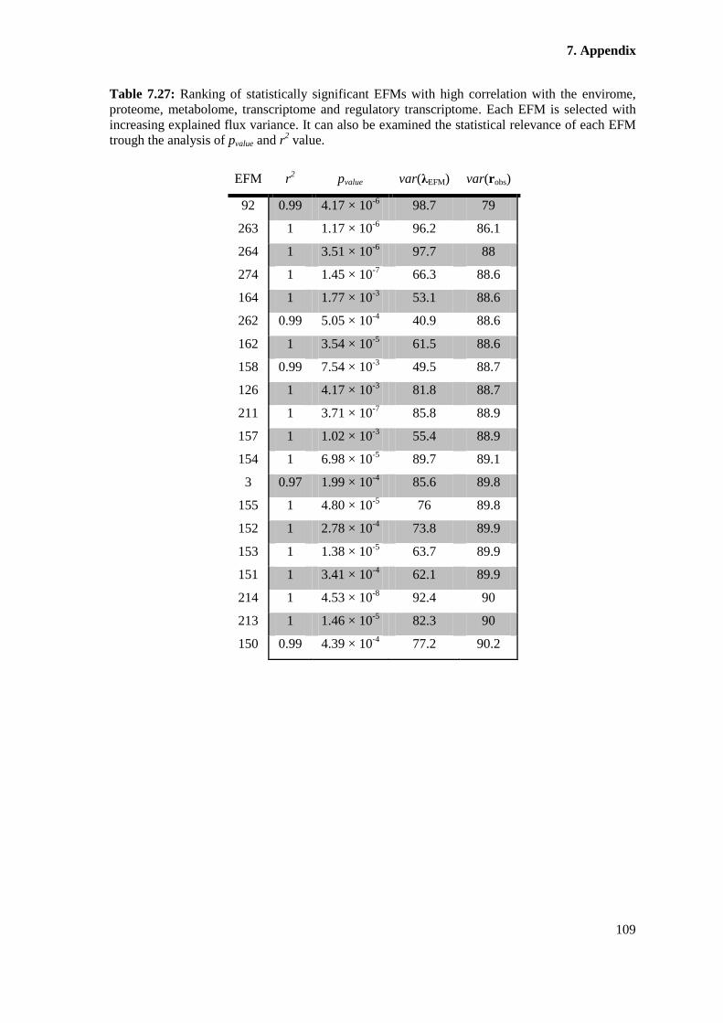
7. Appendix
109
Table 7.27: Ranking of statistically significant EFMs with high correlation with the envirome,
proteome, metabolome, transcriptome and regulatory transcriptome. Each EFM is selected with
increasing explained flux variance. It can also be examined the statistical relevance of each EFM
trough the analysis of pvalue and r2 value.
EFM r2 pvalue var(λEFM) var(robs)
92 0.99 4.17 × 10⁻⁶
98.7 79
263 1 1.17 × 10⁻⁶
96.2 86.1
264 1 3.51 × 10⁻⁶
97.7 88
274 1 1.45 × 10⁻⁷
66.3 88.6
164 1 1.77 × 10⁻³
53.1 88.6
262 0.99 5.05 × 10⁻⁴
40.9 88.6
162 1 3.54 × 10⁻⁵
61.5 88.6
158 0.99 7.54 × 10⁻³
49.5 88.7
126 1 4.17 × 10⁻³
81.8 88.7
211 1 3.71 × 10⁻⁷
85.8 88.9
157 1 1.02 × 10⁻³
55.4 88.9
154 1 6.98 × 10⁻⁵
89.7 89.1
3 0.97 1.99 × 10⁻⁴
85.6 89.8
155 1 4.80 × 10⁻⁵
76 89.8
152 1 2.78 × 10⁻⁴
73.8 89.9
153 1 1.38 × 10⁻⁵
63.7 89.9
151 1 3.41 × 10⁻⁴
62.1 89.9
214 1 4.53 × 10⁻⁸
92.4 90
213 1 1.46 × 10⁻⁵
82.3 90
150 0.99 4.39 × 10⁻⁴
77.2 90.2