Hybrid Multiscale Integration for Directionally Scale Separable Problems

Shuhai Zhang∗ and Caglar Oskay†

Department of Civil and Environmental EngineeringVanderbilt UniversityNashville, TN 37235

Abstract

This manuscript presents the formulation and implementation of a hybrid multiscale inte-

gration scheme for multiscale problems that exhibit different scale separation characteristics in

different directions. The proposed approach employs the key ideas of the variational multiscale

enrichment at directions that exhibit poor scale separation and computational homogenization

at directions with good scale separability. The proposed approach is particularly attractive for

surface degradation problems in structures operating in the presence of aggressive environmen-

tal agents. Formulated in the context of variational multiscale principles, we develop a novel

integration scheme that takes advantage of homogenization-like integration along directions

that exhibit scale separation. The proposed integration scheme is applied to the reduced order

variational multiscale enrichment (ROVME) method in order to arrive at a computationally

efficient multiscale solution strategy for surface degradation problems. Numerical verifications

are performed to verify the implementation of the hybrid multiscale integrator. The results

of the verifications reveal high accuracy and computational efficiency, compared with the di-

rect ROVME simulations. A coupled transport-thermo-mechanical analysis is presented to

demonstrate the capability of the proposed computational framework.

Keywords: Multiscale modeling, Reduced order modeling, Variational multiscale enrichment,

Computational homogenization, Hybrid multiscale integration.

∗Department of Civil and Environmental Engineering, Vanderbilt University, Nashville, TN 37235, United States.Email: shuhai.zhang@vanderbilt.edu†Corresponding author address: VU Station B#351831, 2301 Vanderbilt Place, Nashville, TN 37235. Email:

caglar.oskay@vanderbilt.edu

1

1 Introduction

Structures operating in extreme environments subjected to high temperatures and thermo-

mechanical loads often undergo surface degradation induced by the ingress of aggressive en-

vironmental agents. Examples of surface degradation include oxygen embrittlement of metal

alloys in the structural components of high speed aircraft [41, 46], oxygen embrittlement of

ceramic matrix composites [37], and hydrogen embrittlement of metals in hydrogen storage

structures [19], among many others [29, 45]. While the aggressive agent ingress is often lim-

ited to a very small thickness along the exposed surfaces of the structure, materials properties

changes within the affected regions are severe enough to cause significant reduction in strength

and life of the overall structural component [35, 44]. This manuscript develops a computation-

ally efficient, concurrent multiscale computational approach to address surface degradation

problems.

Two categories of multiscale computational methods have emerged based on the concept

of scale separability. Scale separation refers to the discrepancy between the characteristic size

of the fine scale problem (i.e. the size of the heterogeneous representative volume or a unit

cell, lm) and that of the coarse scale problem (e.g., the dominant response feature such as the

plastic process zone, lM ).

In the past few decades, a range of multiscale methods have been proposed to address

those problems that operate at the limit of scale separation (ζ = lm/lM → 0). These in-

clude computational homogenization (also known as FE2) [3, 23], multiscale finite element

method [24, 18], heterogeneous multiscale method [17, 9], among others. In view of the tremen-

dous computational complexity associated with coupled evaluation of problems at multiple

scales, these methods are often employed in conjunction with reduced order modeling such as

Fast Fourier transform [33], proper orthogonal decomposition [47], transformation field analy-

sis [16, 12, 4, 32], eigendeformation-based homogenization (EHM) [40, 49, 50], machine learning

based reduced modeling [8], hyper-reduced modeling [36], among others, particularly in the

presence of nonlinear behavior.

Similarly, a number of global-local methods have been proposed to address problems that

exhibit poor scale separation (ζ = lm/lM ≈ 1). The key idea in these approaches is to resolve

the fine scale behavior at small subdomains of the overall structural domain, whereas a coarse

description (e.g., a coarse discretization and phenomenological modeling) is employed within

the remainder of the domain. Global-local finite element method [34, 31, 21, 22], domain

decomposition methods [30], s-version finite elements [20], generalized finite elements [15],

numerical subgrid algorithms [1, 2] based on the variational multiscale method [25, 27] among

others are examples of global-local methods that employ this principle. More recently, the

authors developed the variational multiscale enrichment (VME) method [38, 39, 48], a variant

2

of the numerical subgrid algorithm, to study problems that exhibit material heterogeneity at

the scale of the material microstructure. This approach relies on the resolution of the fine

scale problems, which is computationally costly for large scale systems. The computational

efficiency of the VME approach has been significantly improved by introducing a reduced order

approximation of the fine scale response based on the EHM principles [40, 49, 50].

Surface degradation problems introduce a challenge to the existing multiscale computa-

tional methods, since they exhibit direction-dependent scale separability. In the direction

normal to the exposed surfaces of the structure, aggressive agent ingress significantly alters

the mechanical response and the resolution of the microstructural heterogeneities and the local

response within this direction is critical to accurately assess the structural state. On the other

hand, the response is self-similar along the transverse directions and the behavior could be

accurately captured using the principles of computational homogenization.

This manuscript presents the formulation and implementation of a hybrid multiscale inte-

gration scheme for problems, where the relevant response fields exhibit different scale separa-

tion characteristics in various directions. The proposed approach employs the key ideas of the

variational multiscale enrichment at directions, where the response fields exhibit poor scale

separation, and the computational homogenization at directions, where the response fields

show good scale separability. The formulation is based on the variational multiscale principles

and develops a novel integration scheme that takes advantage of homogenization-like integra-

tion along directions that exhibit scale separation. The proposed integration scheme is also

integrated with the reduced order variational multiscale enrichment in order to achieve a com-

putationally efficient multiscale solution strategy for surface degradation problems. A suite of

numerical verifications is performed to verify the implementation of the proposed multiscale

scheme. The results of the verification studies indicate that the approach further improves

the efficiency of the ROVME simulations, without significant compromise on accuracy. A cou-

pled transport-thermo-mechanical analysis is presented to demonstrate the capability of the

proposed computational framework.

The remainder of the manuscript is organized as follows: Section 2 provides the variational

multiscale enrichment setting for directionally scale separable problems. The hybrid multiscale

integration scheme is described in Section 3. Section 4 presents the application of the hybrid

multiscale integration to the ROVME method. Section 5 details the hourglassing control of the

proposed approach. Numerical verifications are presented in Section 6. In the context of small

strains and elasto-viscoplastic constitutive behaviors, a coupled transport-thermo-mechanical

problem with surface degradation is presented in Section 7 to demonstrate the capability of

the proposed computational framework. Section 8 discusses the conclusions of this research.

3

x

zα

αXαX

αX

Ѳ

Ω

αZ ...Ѳα

ζ=αXѲ...

Response

Res

pons

e

z

x

uU Ω = Ωb Ωs

Ωb

Ω s t

x’

z’ Γu Γt

Γuα

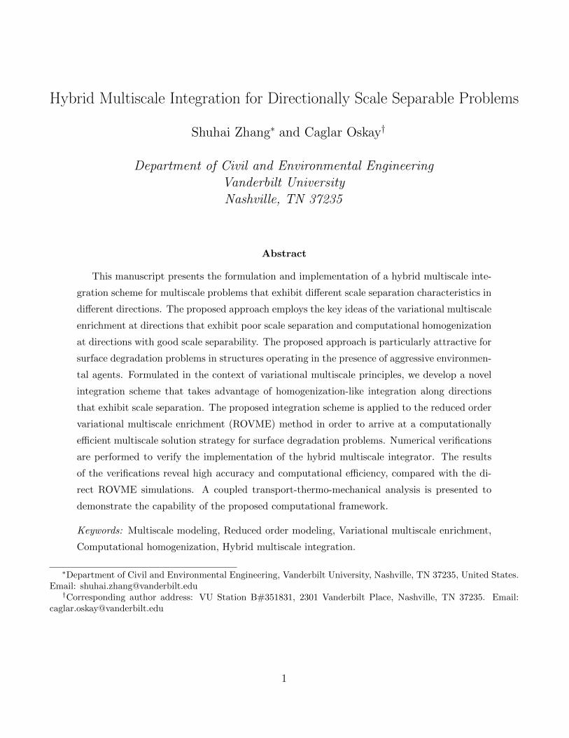
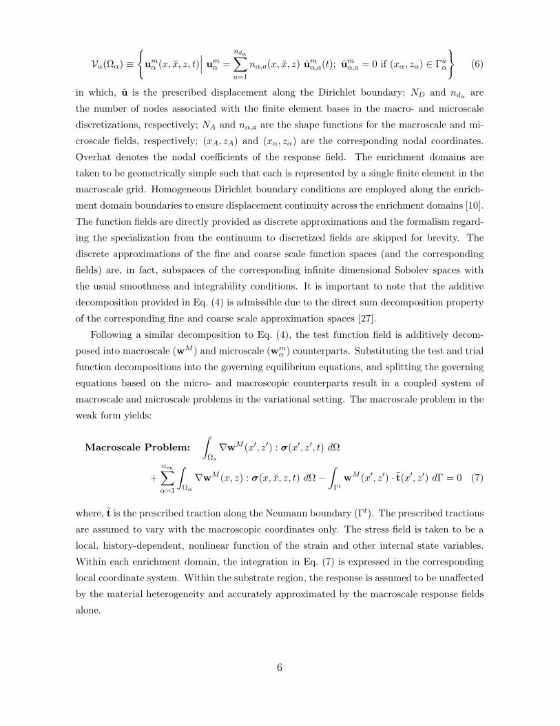
Figure 1: Domain decomposition for directionally scale separable problems

2 Variational multiscale enrichment setting for di-

rectionally scale separable problems

The proposed multiscale approach generalizes and builds on the variational multiscale en-

richment idea introduced in Refs. [48, 49, 50]. Consider an open, bounded Ω ⊂ R2 that

constitutes the domain of the macroscopic structure. The global coordinate system is denoted

by x′ = (x′, z′) as shown in Fig. 1. Under the applied loading and environmental conditions,

the structure undergoes significant localized deformation within a characteristic subdomain,

Ωb ∈ Ω, whereas within the remainder of the domain, Ωs ≡ Ω\Ωb, the response does not local-

ize. We are therefore concerned with accurately and efficiently capturing response fields within

Ωb (i.e., the enrichment region). In surface degradation problems, the enrichment region spans

the boundaries of the structure exposed to aggressive environmental agents but extends to a

very limited depth compared to the overall structural thickness as illustrated in Fig. 1. The

enrichment region is further discretized into a series of non-overlapping enrichment domains

as:

Ωb =

nen⋃α=1

Ωα; Ωα ∩ Ωβ ≡ ∅; α 6= β (1)

in which, nen denotes the total number of enrichment domains in the structure. The enrichment

domain, Ωα is formed by the repetition of a heterogeneous microstructure, Θα along the

4

local direction, x (x′) and the size of the microstructure is taken to be small compared to

the dimension of the enrichment domain along the homogenizable direction, x. In contrast,

the size of the enrichment domain in the normal direction z (x′) is identical to that of the

microstructure. The ratio between the size of the microstructure domain and the enrichment

domain is denoted by a small positive scaling constant, ζ defined as:

ζ =Xθα

Xα→ 0 (2)

in which, Xθα and Xα are the sizes of Θα and Ωα in the x-direction, respectively. The response

within the enrichment domain along x rapidly oscillates in space due to the fluctuations in the

material properties within the microstructure. The response fields are therefore considered to

be functions of the macroscale coordinate system, x, as well as a microscale coordinate system,

x = x/ζ, which is a stretched position vector.

The problem setting described above indicates directional homogenization of the response

fields; i.e., the response fields are scale separable at prescribed directions, whereas they are

taken to be scale inseparable at other directions. We therefore seek to employ the compu-

tational homogenization principles along the scale separable directions, whereas employ the

variational multiscale setting along the scale inseparable direction. Within this problem set-

ting, an arbitrary response field in an enrichment domain is expressed as:

f ζ (x) = f (x, x(x), z) (3)

where, f ζ denotes the response field expressed in the original coordinate system, and super-

script ζ indicates that the field is oscillatory in the scale separable direction.

We start by considering the following additive decomposition of the deformation field [27,

38, 48] within an arbitrary enrichment domain, Ωα:

u(x, x, z, t) = uM (x, z, t) + umα (x, x, z, t) (4)

where, uM ∈ VM (Ω) and umα ∈ Vα(Ωα) are respectively the macroscale and microscale dis-

placement fields; and VM and Vα denote the trial (discretized) spaces for the macro- and

microscale fields, respectively:

VM (Ω) ≡

uM

[x(x′), z(x′), t

] ∣∣∣ uM =

NαD∑

A=1

NA(x′, z′) uMA (t);

uMA = u(x′A, z′A, t) if (x′A, z

′A) ∈ Γu

(5)

5

Vα(Ωα) ≡

umα (x, x, z, t)

∣∣∣ umα =

ndα∑a=1

nα,a(x, x, z) umα,a(t); umα,a = 0 if (xα, zα) ∈ Γuα

(6)

in which, u is the prescribed displacement along the Dirichlet boundary; ND and ndα are

the number of nodes associated with the finite element bases in the macro- and microscale

discretizations, respectively; NA and nα,a are the shape functions for the macroscale and mi-

croscale fields, respectively; (xA, zA) and (xα, zα) are the corresponding nodal coordinates.

Overhat denotes the nodal coefficients of the response field. The enrichment domains are

taken to be geometrically simple such that each is represented by a single finite element in the

macroscale grid. Homogeneous Dirichlet boundary conditions are employed along the enrich-

ment domain boundaries to ensure displacement continuity across the enrichment domains [10].

The function fields are directly provided as discrete approximations and the formalism regard-

ing the specialization from the continuum to discretized fields are skipped for brevity. The

discrete approximations of the fine and coarse scale function spaces (and the corresponding

fields) are, in fact, subspaces of the corresponding infinite dimensional Sobolev spaces with

the usual smoothness and integrability conditions. It is important to note that the additive

decomposition provided in Eq. (4) is admissible due to the direct sum decomposition property

of the corresponding fine and coarse scale approximation spaces [27].

Following a similar decomposition to Eq. (4), the test function field is additively decom-

posed into macroscale (wM ) and microscale (wmα ) counterparts. Substituting the test and trial

function decompositions into the governing equilibrium equations, and splitting the governing

equations based on the micro- and macroscopic counterparts result in a coupled system of

macroscale and microscale problems in the variational setting. The macroscale problem in the

weak form yields:

Macroscale Problem:

∫Ωs

∇wM (x′, z′) : σ(x′, z′, t) dΩ

+

nen∑α=1

∫Ωα

∇wM (x, z) : σ(x, x, z, t) dΩ−∫

ΓtwM (x′, z′) · t(x′, z′) dΓ = 0 (7)

where, t is the prescribed traction along the Neumann boundary (Γt). The prescribed tractions

are assumed to vary with the macroscopic coordinates only. The stress field is taken to be a

local, history-dependent, nonlinear function of the strain and other internal state variables.

Within each enrichment domain, the integration in Eq. (7) is expressed in the corresponding

local coordinate system. Within the substrate region, the response is assumed to be unaffected

by the material heterogeneity and accurately approximated by the macroscale response fields

alone.

6

1

2

3

4α

αXѲα

Ѳ

Ω

αZ

...

...Ѳα

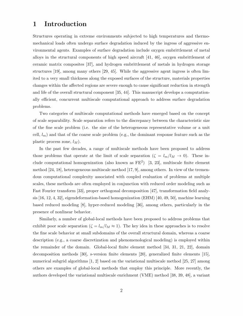
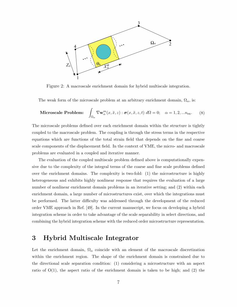
Figure 2: A macroscale enrichment domain for hybrid multiscale integration.

The weak form of the microscale problem at an arbitrary enrichment domain, Ωα, is:

Microscale Problem:

∫Ωα

∇wmα (x, x, z) : σ(x, x, z, t) dΩ = 0; α = 1, 2, ...nen. (8)

The microscale problems defined over each enrichment domain within the structure is tightly

coupled to the macroscale problem. The coupling is through the stress terms in the respective

equations which are functions of the total strain field that depends on the fine and coarse

scale components of the displacement field. In the context of VME, the micro- and macroscale

problems are evaluated in a coupled and iterative manner.

The evaluation of the coupled multiscale problem defined above is computationally expen-

sive due to the complexity of the integral terms of the coarse and fine scale problems defined

over the enrichment domains. The complexity is two-fold: (1) the microstructure is highly

heterogeneous and exhibits highly nonlinear response that requires the evaluation of a large

number of nonlinear enrichment domain problems in an iterative setting; and (2) within each

enrichment domain, a large number of microstructures exist, over which the integrations must

be performed. The latter difficulty was addressed through the development of the reduced

order VME approach in Ref. [49]. In the current manuscript, we focus on developing a hybrid

integration scheme in order to take advantage of the scale separability in select directions, and

combining the hybrid integration scheme with the reduced order microstructure representation.

3 Hybrid Multiscale Integrator

Let the enrichment domain, Ωα coincide with an element of the macroscale discretization

within the enrichment region. The shape of the enrichment domain is constrained due to

the directional scale separation condition: (1) considering a microstructure with an aspect

ratio of O(1), the aspect ratio of the enrichment domain is taken to be high; and (2) the

7

element length in the scale inseparable direction is taken to be constant and equal to the

edge length of the microstructure along the same direction. Define vectors vij = x′j − x′i =

(x′j , z′j)− (x′i, z

′i); i, j = 1, 2, 3, 4; i 6= j within the enrichment domain. Denoting the size of the

microstructure in the scale separable direction as Xθα and in the scale inseparable direction as

Zθα, the above-mentioned constraints are imposed as follows:

(i) v12//v34 ( i.e., |(v12 · v34)/(||v12|| ||v34||)| = 1), and;

ζ =2Xθ

α

‖ v12 ‖ + ‖ v34 ‖→ 0; Zθα = Zα ≡ |v23 · vn| (9)

where, vn ⊥ v12 and vn is a unit vector, or;

(ii) v23//v41 (i.e., |(v23 · v41)/(||v23|| ||v41||)| = 1), and;

ζ =2Xθ

α

‖ v23 ‖ + ‖ v41 ‖→ 0; Zθα = Zα ≡ |v12 · vn|; vn ⊥ v23. (10)

where, (·)//(∗) indicates (·) parallels to (∗), ‖ (·) ‖ denotes the norm of a vector (·) and |(∗)| isthe absolute value of a scalar (∗). When (i) or (ii) is satisfied, such as in the example shown in

Fig. 2, the enrichment domain is scale separable, and the hybrid multiscale integration scheme

described below is applicable.

3.1 Canonical coordinate systems

In context of standard finite element coordinate system transformation, the macroscale prob-

lem for an enrichment domain is first transfered from the global coordinate system (x′) to a

standard canonical system (ξ). Then, the response discretization in Eq. (5) is performed using

the standard shape functions in the canonical system. In the current setting, a new set of

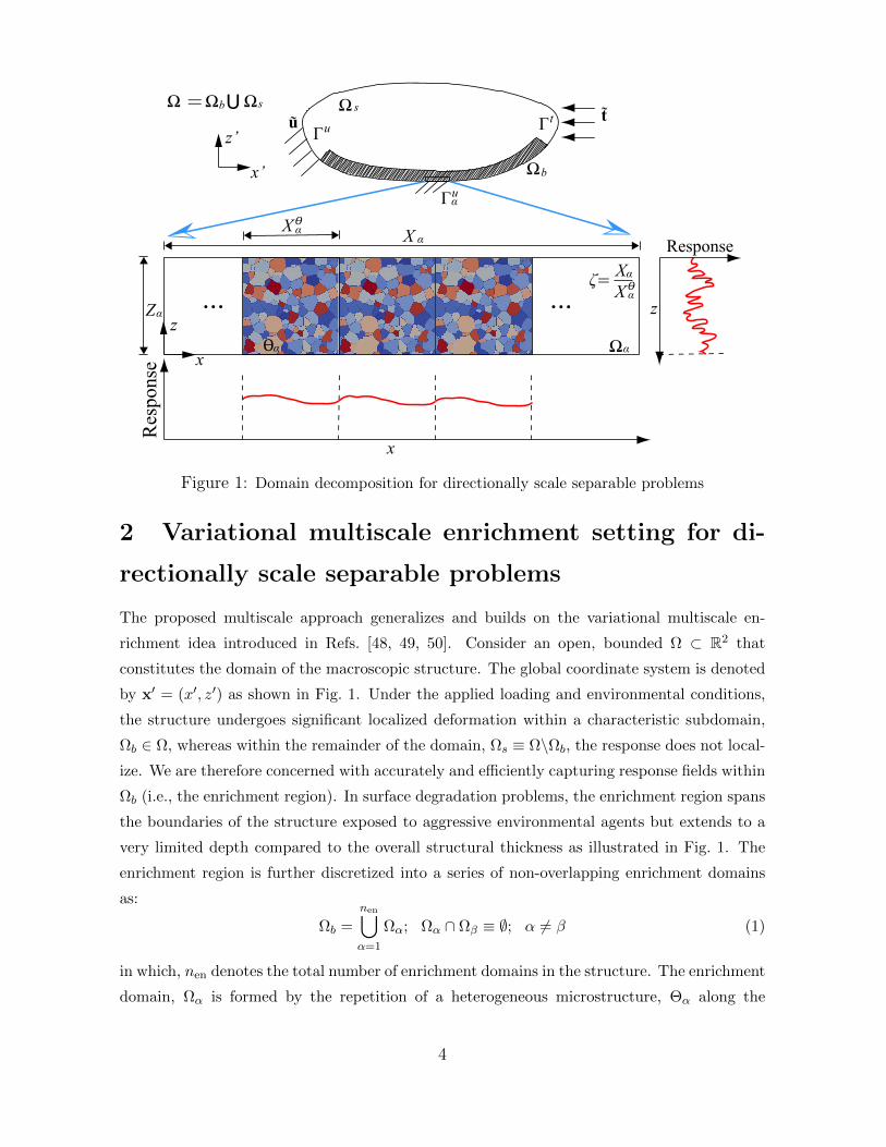
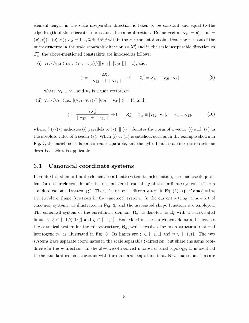
canonical systems, as illustrated in Fig. 3, and the associated shape functions are employed.

The canonical system of the enrichment domain, Ωα, is denoted as ξ with the associated

limits as ξ ∈ [−1/ζ, 1/ζ] and η ∈ [−1, 1]. Embedded in the enrichment domain, denotes

the canonical system for the microstructure, Θα, which resolves the microstructural material

heterogeneity, as illustrated in Fig. 3. Its limits are ξ ∈ [−1, 1] and η ∈ [−1, 1]. The two

systems have separate coordinates in the scale separable ξ-direction, but share the same coor-

dinate in the η-direction. In the absence of resolved microstructural topology, is identical

to the standard canonical system with the standard shape functions. New shape functions are

8

(a)

ξ

η

1 (-1/ζ, -1) 2 (1/ζ, -1)

3 (1/ζ, 1)4 (-1/ζ, 1)

ξ

η4(-1, 1) 3(1, 1)

1(-1, -1) 2(1, -1)(b)

ξ

Figure 3: Canonical systems of the hybrid integration for: (a) the enrichment domainand (b) the microstructure of the enrichment domain.

defined for ξ as:

N1(ξ, η; ζ) =(1− ζ ξ)(1− η)

4; N2(ξ, η; ζ) =

(1 + ζ ξ)(1− η)

4

N3(ξ, η; ζ) =(1 + ζ ξ)(1 + η)

4; N4(ξ, η; ζ) =

(1− ζ ξ)(1 + η)

4.

(11)

The hybrid integrations for the micro- and macroscale problems over the enrichment domains

are performed by considering the canonical systems in Fig. 3 and their shape functions.

3.2 Integration of macroscale and microscale problems

We first demonstrate the proposed hybrid multiscale integration over a scalar function, ψ.

The integration scheme is then applied to the enrichment domain integrals that appear in the

microscale and macroscale problems. Let ψ be sufficiently smooth and integrable function

over the enrichment domain. The function is assumed to be periodic along the homogenizable

direction, x. Considering coordinate transformation and the homogenization concept in the

ξ-direction as ζ → 0 [23], the integration of ψ over Ωα is expressed as follows:

limζ→0

∫Ωα

ψ(x, x =x

ζ, z) dΩ = lim

ζ→0

∫ 1

−1

∫ 1ζ

− 1ζ

ψ(ξ, ξ, η) detJ(ξ, η) dξ dη

=

∫ 1

−1

∫ 1ζ

− 1ζ

ψ(ξ, η) detJ(ξ, η) dξ dη

(12)

9

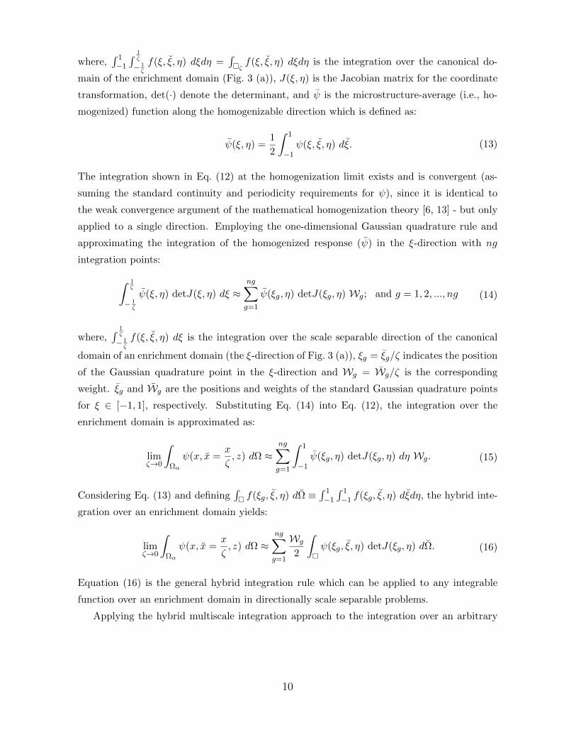
where,∫ 1−1

∫ 1ζ

− 1ζ

f(ξ, ξ, η) dξdη =∫ζf(ξ, ξ, η) dξdη is the integration over the canonical do-

main of the enrichment domain (Fig. 3 (a)), J(ξ, η) is the Jacobian matrix for the coordinate

transformation, det(·) denote the determinant, and ψ is the microstructure-average (i.e., ho-

mogenized) function along the homogenizable direction which is defined as:

ψ(ξ, η) =1

2

∫ 1

−1ψ(ξ, ξ, η) dξ. (13)

The integration shown in Eq. (12) at the homogenization limit exists and is convergent (as-

suming the standard continuity and periodicity requirements for ψ), since it is identical to

the weak convergence argument of the mathematical homogenization theory [6, 13] - but only

applied to a single direction. Employing the one-dimensional Gaussian quadrature rule and

approximating the integration of the homogenized response (ψ) in the ξ-direction with ng

integration points:

∫ 1ζ

− 1ζ

ψ(ξ, η) detJ(ξ, η) dξ ≈ng∑g=1

ψ(ξg, η) detJ(ξg, η) Wg; and g = 1, 2, ..., ng (14)

where,∫ 1ζ

− 1ζ

f(ξ, ξ, η) dξ is the integration over the scale separable direction of the canonical

domain of an enrichment domain (the ξ-direction of Fig. 3 (a)), ξg = ξg/ζ indicates the position

of the Gaussian quadrature point in the ξ-direction and Wg = Wg/ζ is the corresponding

weight. ξg and Wg are the positions and weights of the standard Gaussian quadrature points

for ξ ∈ [−1, 1], respectively. Substituting Eq. (14) into Eq. (12), the integration over the

enrichment domain is approximated as:

limζ→0

∫Ωα

ψ(x, x =x

ζ, z) dΩ ≈

ng∑g=1

∫ 1

−1ψ(ξg, η) detJ(ξg, η) dη Wg. (15)

Considering Eq. (13) and defining∫ f(ξg, ξ, η) dΩ ≡

∫ 1−1

∫ 1−1 f(ξg, ξ, η) dξdη, the hybrid inte-

gration over an enrichment domain yields:

limζ→0

∫Ωα

ψ(x, x =x

ζ, z) dΩ ≈

ng∑g=1

Wg

2

∫ψ(ξg, ξ, η) detJ(ξg, η) dΩ. (16)

Equation (16) is the general hybrid integration rule which can be applied to any integrable

function over an enrichment domain in directionally scale separable problems.

Applying the hybrid multiscale integration approach to the integration over an arbitrary

10

enrichment domain of the macroscale problem (Eq. (7)) yields the following expression:

limζ→0

∫Ωα

∇wM (x, z) : σ(x, x, z, t) dΩ

≈ng∑g=1

Wαg

2

∫∇wM (ξαg, η) : σ(ξαg, ξ, η, t) detJ(ξαg, η) dΩ

(17)

where, ξαg and Wαg are the positions and associated weights for the enrichment domain, Ωα.

Similarly, the microscale weak form for the enrichment domain Ωα (Eq. (8)) is obtained as:

limζ→0

∫Ωα

∇wmα (x, x, z) : σ(x, x, z, t) dΩ

≈ng∑g=1

Wαg

2

∫∇wm

α (ξαg, ξ, η) : σ(ξαg, ξ, η, t) detJ(ξαg, η) dΩ = 0.

(18)

SinceWαg does not depend on ξ or η, a solution that ensures the equilibrium of the microscale

state (Eq. (18)) is:∫∇wm

α (ξαg, ξ, η) : σ(ξαg, ξ, η, t) detJ(ξαg, η) dΩ = 0; ∀g = 1, 2, ..., ng. (19)

Equation (19) implies that under the condition of directional scale-separability, enforcement

of equilibrium at the scale of the microstructure associated with each quadrature point implies

the microscale equilibrium within the enrichment domain. Equations (18) and (19)) represent

the integration over an arbitrary enrichment domain (Eq. (7)) which consists of: 1) a two-scale

integration along the scale separable direction (ξαg and ξ represents macroscale and microscale,

respectively); and 2) a single scale integration (η) performed along the scale inseparable di-

rection. The application of the hybrid multiscale integration to the micro- and macroscale

problems requires that the fine scale components of the response fields over the microstructure

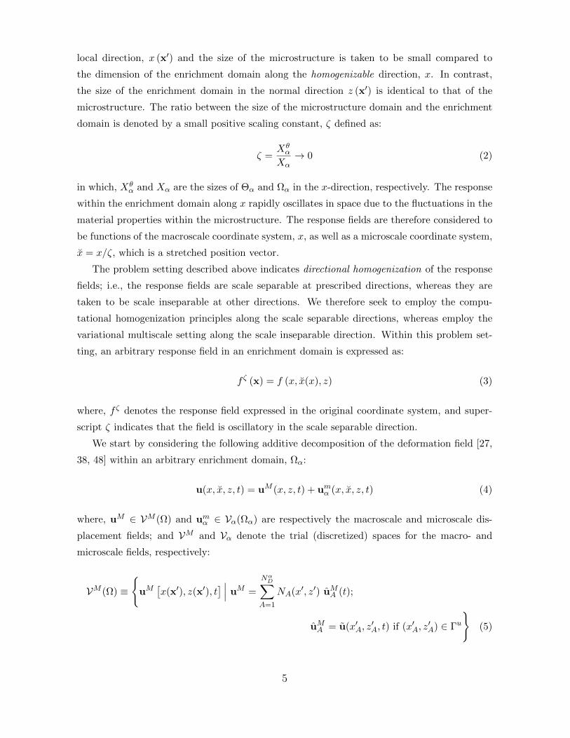
are periodic along the η-direction. In order to ensure continuity across neighboring enrichment

domains or along the boundaries between the enrichment domains and the substrate [38, 48],

homogeneous Dirichlet boundary conditions are prescribed for microstructure boundaries along

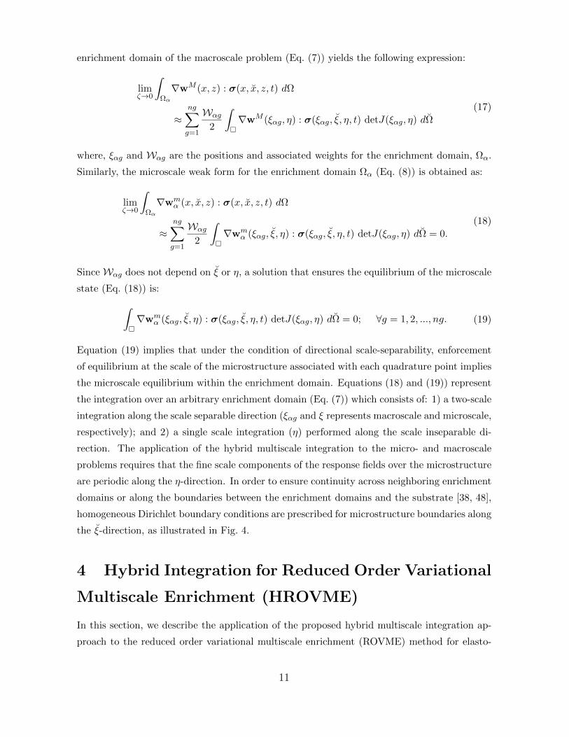
the ξ-direction, as illustrated in Fig. 4.

4 Hybrid Integration for Reduced Order Variational

Multiscale Enrichment (HROVME)

In this section, we describe the application of the proposed hybrid multiscale integration ap-

proach to the reduced order variational multiscale enrichment (ROVME) method for elasto-

11

αξη

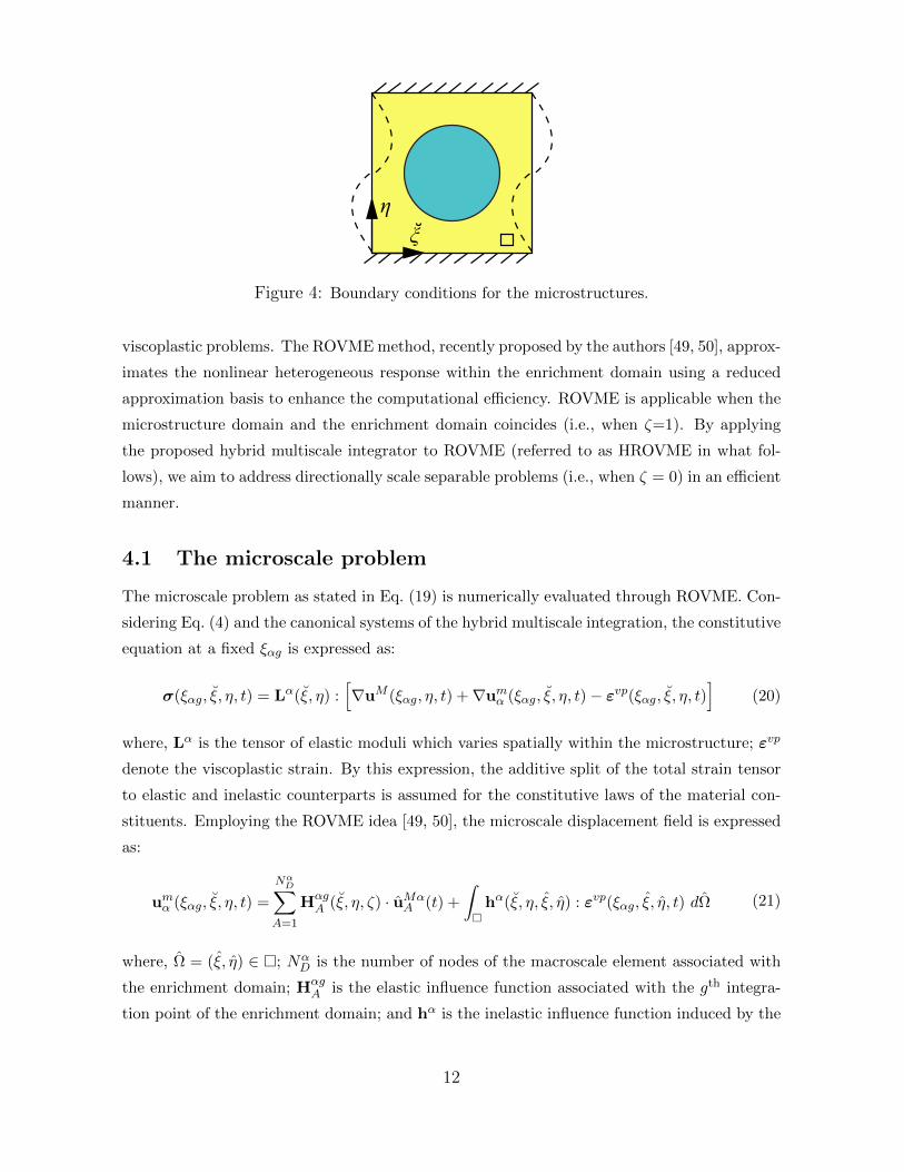
Figure 4: Boundary conditions for the microstructures.

viscoplastic problems. The ROVME method, recently proposed by the authors [49, 50], approx-

imates the nonlinear heterogeneous response within the enrichment domain using a reduced

approximation basis to enhance the computational efficiency. ROVME is applicable when the

microstructure domain and the enrichment domain coincides (i.e., when ζ=1). By applying

the proposed hybrid multiscale integrator to ROVME (referred to as HROVME in what fol-

lows), we aim to address directionally scale separable problems (i.e., when ζ = 0) in an efficient

manner.

4.1 The microscale problem

The microscale problem as stated in Eq. (19) is numerically evaluated through ROVME. Con-

sidering Eq. (4) and the canonical systems of the hybrid multiscale integration, the constitutive

equation at a fixed ξαg is expressed as:

σ(ξαg, ξ, η, t) = Lα(ξ, η) :[∇uM (ξαg, η, t) +∇umα (ξαg, ξ, η, t)− εvp(ξαg, ξ, η, t)

](20)

where, Lα is the tensor of elastic moduli which varies spatially within the microstructure; εvp

denote the viscoplastic strain. By this expression, the additive split of the total strain tensor

to elastic and inelastic counterparts is assumed for the constitutive laws of the material con-

stituents. Employing the ROVME idea [49, 50], the microscale displacement field is expressed

as:

umα (ξαg, ξ, η, t) =

NαD∑

A=1

HαgA (ξ, η, ζ) · uMα

A (t) +

∫

hα(ξ, η, ξ, η) : εvp(ξαg, ξ, η, t) dΩ (21)

where, Ω = (ξ, η) ∈ ; NαD is the number of nodes of the macroscale element associated with

the enrichment domain; HαgA is the elastic influence function associated with the gth integra-

tion point of the enrichment domain; and hα is the inelastic influence function induced by the

12

inelastic behavior within the microstructure. The influence functions are approximations to

Green’s function problems defined over the microstructure, and evaluated numerically. With

a slight deviation from the ROVME approach, the influence functions are evaluated by con-

sidering the semi-periodic boundary conditions described above. Considering element level

discretization of the macroscale displacement field through the ζ-dependent shape functions

in Eq. (11):

uM (ξαg, η, t) =

NαD∑

A=1

NA(ξαg, η, ζ, t) uMαA (t) (22)

and, substituting the constitutive equation (Eq. (20)), macro- and microscale displacement

discretizations (Eqs. (21) and (22)) into Eq. (19), the microscale problem in weak form yields:

NαD∑

A=1

[ ∫∇wm

αg(ξ, η) : Lα(ξ, η) · ∇NA(ξαg, η, ζ) detJ(ξαg, η) dΩ

+

∫∇wm

αg(ξ, η) : Lα(ξ, η) : ∇HαgA (ξ, η, ζ) detJ(ξαg, η) dΩ

]· uMα

A (t)

+

∫∇wm

αg(ξ, η) : Lα(ξ, η) :

[ ∫∇hα(ξ, η, ξ, η) : εvp(ξαg, ξ, η, t) dΩ

− εvp(ξαg, ξ, η, t)]

detJ(ξαg, η) dΩ = 0 (23)

where, ∇wmαg(ξ, η) ≡ ∇wm

α (ξαg, ξ, η). Considering the case when the microstructure deforms

elastically (εvp = 0), Eq. (23) yields the elastic influence function problem that can be solved

for HαgA :

∫∇wm

αg(ξ, η) : Lα(ξ, η) : ∇HαgA (ξ, η, ζ) detJ(ξαg, η) dΩ =

−∫∇wm

αg(ξ, η) : Lα(ξ, η) · ∇NA(ξαg, η, ζ) detJ(ξαg, η) dΩ;

∀A = 1, 2, ..., NαD and g = 1, 2, ..., ng. (24)

Substituting Eq. (24) into the microscale weak form (Eq. (23)), results in the inelastic influence

function problem for hα:∫∇wm

αg(ξ, η) :Lα(ξ, η) : ∇hα(ξ, η, ξ, η) detJ(ξαg, η) dΩ =∫∇wm

αg(ξ, η) : Lα(ξ, η) δd(ξ − ξ, η − η) detJ(ξαg, η) dΩ; ∀(ξ, η) ∈ (25)

in which, δd denotes the Dirac delta distribution. The elastic and inelastic microscale influence

function problems are linear elastic problems defined over the microstructure. Therefore, the

13

influence functions are computed off-line, prior to a macroscale analysis.

Next, a microstructure partitioning is considered to obtain a reduced order approximation

to the microscale problems [40, 49, 50]. The microstructure defined in the canonical form is

decomposed into NP non-overlapping subdomains (i.e., parts):

=NP⋃γ=1

γ ; γ ∩λ ≡ ∅ when γ 6= λ (26)

where, γ denotes a part of the microstructure. Stress and inelastic strain fields within the

microstructure are then expressed as:

σ(ξαg, ξ, η, t) =NP∑γ=1

Nγ(ξ, η) σαgγ (t); εvp(ξαg, ξ, η, t) =NP∑γ=1

Nγ(ξ, η) µαgγ (t) (27)

where, Nγ(ξ, η) denotes a reduced model shape function:

Nγ(ξ, η) =

1, if (ξ, η) ∈ γ

0, elsewhere .(28)

The stress and inelastic strain fields are therefore approximated as spatially piecewise constant

fields with unknown coefficients , σαgγ and µαgγ , respectively. Substituting Eq. (27) into Eq. (20)

and using Eq. (28), the constitutive equation is expressed in terms of the unknown stress and

inelastic coefficients as:

σαgλ (t) =

NαD∑

A=1

SαgλA(ζ) · uMαA (t) +

NP∑γ=1

Pαλγ : µαgγ (t) (29)

where,

SαgλA(ζ) =1

|Θαλ |

∫Θαgλ

[Lα(ξ, η) · ∇NA(ξαg, η, ζ) + Lα(ξ, η) : ∇Hαg

A (ξ, η, ζ)]dΩ (30)

Pαλγ =

1

|Θαλ |

∫Θαgλ

[Lα(ξ, η) :

∫Θαgγ

∇hα(ξ, η, ξ, η) dΩ− Lα(ξ, η) Nγ(ξ, η)

]dΩ. (31)

Equation (29) along with the evolution equations for viscoplastic slip defined for inelastic strain

coefficients (µαgγ ) constitute a nonlinear, history dependent system of equations that are eval-

uated for the inelastic strain and stress coefficients for a prescribed macroscopic deformation

state (uMα) within the enrichment domain.

Remark 1. The reduced basis approximation of the microscale problem has the following

14

characteristics: (1) The order of the reduced basis is of NP . The number of parts is taken

to be much smaller compared to the number of degrees of freedom in a typical finite element

discretization of the microstructure domain. (2) The coefficient tensors (S and P) are functions

of the elastic properties of the microstructure constituents, the influence functions (H and h),

and the scaling parameter, ζ, as shown in Eqs. (30) and (31). For a fixed scaling constant,

the coefficient tensors are therefore computable a-priori, similar to the influence functions. In

contrast, macroscopic discretization could include enrichment domains with varying element

lengths (i.e., varying scaling constants). The Appendix provides an analytical relationship for

computing the coefficient tensors for an arbitrary scaling constant from those pre-computed for

a reference scaling constant. This analytical relationship is significant, since by this approach,

a single set of coefficient tensors is stored for all enrichment domains regardless of shape.

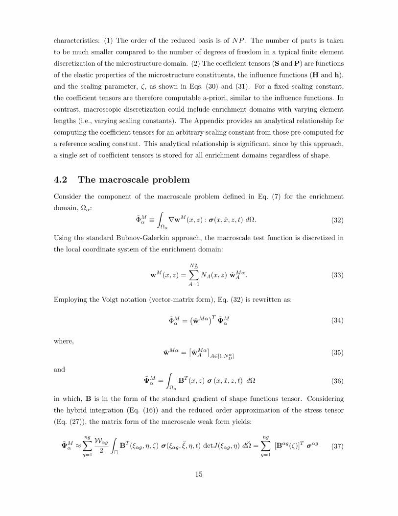
4.2 The macroscale problem

Consider the component of the macroscale problem defined in Eq. (7) for the enrichment

domain, Ωα:

ΦMα ≡

∫Ωα

∇wM (x, z) : σ(x, x, z, t) dΩ. (32)

Using the standard Bubnov-Galerkin approach, the macroscale test function is discretized in

the local coordinate system of the enrichment domain:

wM (x, z) =

NαD∑

A=1

NA(x, z) wMαA . (33)

Employing the Voigt notation (vector-matrix form), Eq. (32) is rewritten as:

ΦMα =

(wMα

)TΨMα (34)

where,

wMα =[wMαA

]A∈[1,Nα

D](35)

and

ΨMα =

∫Ωα

BT (x, z) σ (x, x, z, t) dΩ (36)

in which, B is in the form of the standard gradient of shape functions tensor. Considering

the hybrid integration (Eq. (16)) and the reduced order approximation of the stress tensor

(Eq. (27)), the matrix form of the macroscale weak form yields:

ΨMα ≈

ng∑g=1

Wαg

2

∫

BT (ξαg, η, ζ) σ(ξαg, ξ, η, t) detJ(ξαg, η) dΩ =

ng∑g=1

[Bαg(ζ)]T σαg (37)

15

where,

Bαg(ζ) =[Bαgγ (ζ)

]γ∈[1,NP ]

; Bαgγ (ζ) =

Wαg

2

∫γ

B(ξαg, η, ζ) detJ(ξαg, η) dΩ (38)

and

σαg =[σαgγ (t)

]γ∈[1,NP ]

. (39)

Similar to the coefficient tensors S and P, B is a function of the scaling constant, ζ. By

employing the relationship shown in the Appendix, B for an arbitrary scaling constant is

evaluated directly from a B matrix pre-computed for a reference scaling constant.

Considering the discretization of the macroscale weak form over the entire macroscopic

domain (Eq. (7)), the macrocale system of equations in the global coordinate system is defined

as:

Ψ′M ≡A

eΨ′

Me = 0; ∀ Ωe ∈ Ω (40)

where, A is the standard finite element assembly operator. For each enrichment domain,

Ωe ∈ Ωα|α = 1, 2, ..., nen, the residual in the global coordinate system is obtained from that

defined in the local coordinate system of the enrichment domain:

Ψ′Me = Ψ′

Mα = R ΨM

α ; Ωe ∈ Ωα(α = 1, 2, ..., nen) (41)

in which, R is the coordinate rotation tensor between the enrichment domain (x) and the

global coordinate system (x′). The residual of the macroscale weak form in the local coordinate

system is expressed as:

ΨMα ≡ ΨM

α − ΨMTα (42)

where, ΨMα is described in Eq. (37) and:

ΨMTα =

∫Γtα

NM (x, z) · t dΓ (43)

where, NM denotes the standard shape function matrix in Voigt notation. Γtα is the part of

the enrichment domain boundary that intersects with the Neumann boundary of the problem

domain (Γtα ≡ Γα ∩ Γt), in the absence of the microscale displacement field contribution.

For macroscale elements that discretize the substrate region (Ωe ∈ Ωs), the residual of the

macroscale weak form is expressed as:

Ψ′Me = Ψ′

Ms ≡ Ψ′

Ms − Ψ′

MTs ; Ωe ∈ Ωs (44)

16

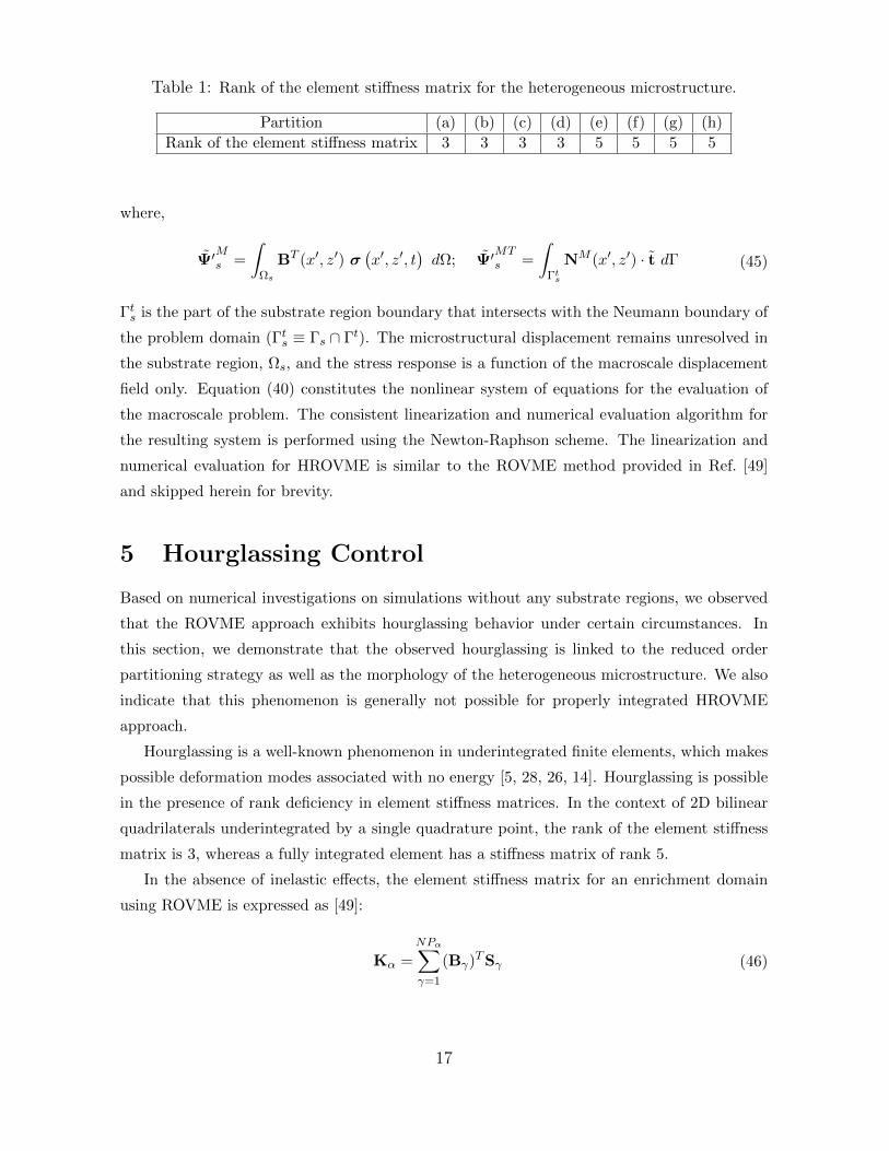
Table 1: Rank of the element stiffness matrix for the heterogeneous microstructure.

Partition (a) (b) (c) (d) (e) (f) (g) (h)

Rank of the element stiffness matrix 3 3 3 3 5 5 5 5

where,

Ψ′Ms =

∫Ωs

BT (x′, z′) σ(x′, z′, t

)dΩ; Ψ′

MTs =

∫Γts

NM (x′, z′) · t dΓ (45)

Γts is the part of the substrate region boundary that intersects with the Neumann boundary of

the problem domain (Γts ≡ Γs ∩ Γt). The microstructural displacement remains unresolved in

the substrate region, Ωs, and the stress response is a function of the macroscale displacement

field only. Equation (40) constitutes the nonlinear system of equations for the evaluation of

the macroscale problem. The consistent linearization and numerical evaluation algorithm for

the resulting system is performed using the Newton-Raphson scheme. The linearization and

numerical evaluation for HROVME is similar to the ROVME method provided in Ref. [49]

and skipped herein for brevity.

5 Hourglassing Control

Based on numerical investigations on simulations without any substrate regions, we observed

that the ROVME approach exhibits hourglassing behavior under certain circumstances. In

this section, we demonstrate that the observed hourglassing is linked to the reduced order

partitioning strategy as well as the morphology of the heterogeneous microstructure. We also

indicate that this phenomenon is generally not possible for properly integrated HROVME

approach.

Hourglassing is a well-known phenomenon in underintegrated finite elements, which makes

possible deformation modes associated with no energy [5, 28, 26, 14]. Hourglassing is possible

in the presence of rank deficiency in element stiffness matrices. In the context of 2D bilinear

quadrilaterals underintegrated by a single quadrature point, the rank of the element stiffness

matrix is 3, whereas a fully integrated element has a stiffness matrix of rank 5.

In the absence of inelastic effects, the element stiffness matrix for an enrichment domain

using ROVME is expressed as [49]:

Kα =

NPα∑γ=1

(Bγ)TSγ (46)

17

(c) (d)

7

1

2

2

3 3

4 4

44

1

2

2

3 3

4

4

4

4

5

5

66

7 7

7

(b)

1

23

(f)

1

3

2

4(e)

1

2

3

(g)

1 2

3 4

5 6

7 8

(h)

129

10

345

678

11

12

13

1415

16

(a)

1

2

Figure 5: Partition patterns of a heterogeneous microstructure.

where,

Bγ =

[∫Ωαγ

∇NA dΩ

]A∈[1,ND]

(47)

Sγ =

[1

|Ωαγ |

∫Ωαγ

L · ∇NA + L : ∇HαgA dΩ

]A∈[1,ND]

. (48)

In order to demonstrate the occurrence of hourglassing in the ROVME approach, we consider

a square unit cell reinforced with a single circular inclusion. The macrostructure is discretized

using a single finite element that constitutes the enrichment domain. Employing eight partition

patterns, the element stiffness matrix for each of them is computed by Eq. (46) and the

corresponding rank is listed in Table 1. The rank deficiency occurs when the centroids of all

the reduced model parts coincide with the centroid of the macroscale element (e.g, partition

pattern (a)-(d)). Indeterminacy in certain deformation modes (hourglassing modes) is a direct

outcome of the rank deficiency. Sufficient ranks are obtained when at least the centroid of

one of the parts is not located at the center of the element (e.g, partition pattern (e)-(h)).

Therefore, reduced order model partitioning, where the centroids of parts coincide, should be

avoided. Some additional approaches previously employed for identifying the partitioning of

the microstructure into reduced bases are discussed in Refs. [42, 43].

The hybrid integration for reduced order variational multiscale enrichment method avoids

the hourglassing instabilities using Eq. (37) with ng > 1. Since the partition pattern of each

of the microstructure, Θαg (g = 1, 2, ..., ng), is independent of the other microstructures (as

18

αѲα Ω

......Ѳ1

......Ѳ2

(a)

1

2

3

4

αѲα Ω

......Ѳ1

......Ѳ2

(b)

1

2

4

5

3 6

Figure 6: Partition patterns of an HROVME heterogeneous enrichment domain withng = 2.

Table 2: Materials parameters for phase II material in the microstructure.

E [GPa] ν A [MPa] B [MPa]

120.8 0.32 895 125

m n γ [MPa/second] q

0.85 0.2 20 1.0

shown in Fig. 6 for ng ≥ 2), it is impossible for the centroid of all parts in the enrichment

domain to coincide with the center of the enrichment domain. None of the macroscale elements

in Fig. 6 demonstrated the hourglassing instability issue when employed through the HROVME

method.

6 Numerical Verification

The implementation of the proposed approach is verified through numerical simulations un-

der the 2-D plane strain condition. The performance and accuracy characteristics of the

hybrid multiscale integration are assessed by comparing the results with the direct ROVME

method [49, 50]. The microstructure is taken to be a two-phase particulate composite with

circular inclusions as shown in Fig. 7(b). Phase I (particle) is taken to be elastic with Young’s

modulus (E) of 395 GPa and Poisson’s ratio (ν) of 0.25, where phase II matrix behaves

elasto-viscoplastically. The viscoplasticity model for the matrix material relies on the Perzyna

19

αΩ

(b)

0.1 mm

0.1 mm

pθ

(a)x

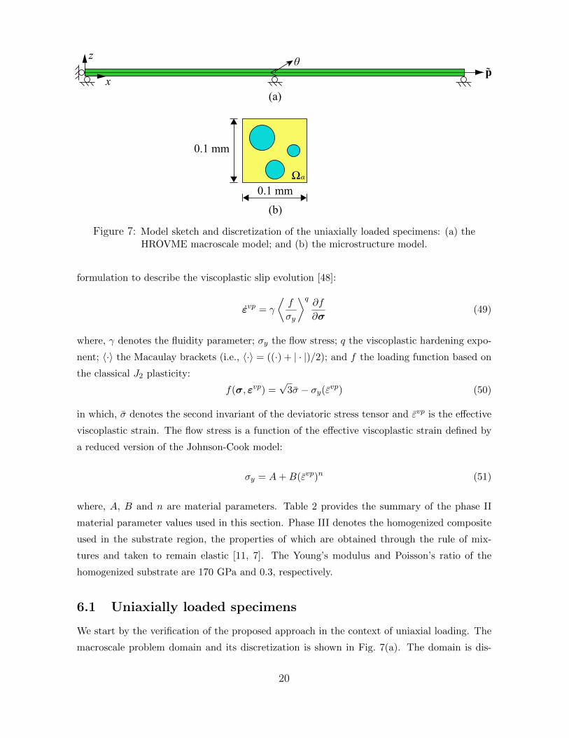
z

Figure 7: Model sketch and discretization of the uniaxially loaded specimens: (a) theHROVME macroscale model; and (b) the microstructure model.

formulation to describe the viscoplastic slip evolution [48]:

εvp = γ

⟨f

σy

⟩q ∂f∂σ

(49)

where, γ denotes the fluidity parameter; σy the flow stress; q the viscoplastic hardening expo-

nent; 〈·〉 the Macaulay brackets (i.e., 〈·〉 = ((·) + | · |)/2); and f the loading function based on

the classical J2 plasticity:

f(σ, εvp) =√

3σ − σy(εvp) (50)

in which, σ denotes the second invariant of the deviatoric stress tensor and εvp is the effective

viscoplastic strain. The flow stress is a function of the effective viscoplastic strain defined by

a reduced version of the Johnson-Cook model:

σy = A+B(εvp)n (51)

where, A, B and n are material parameters. Table 2 provides the summary of the phase II

material parameter values used in this section. Phase III denotes the homogenized composite

used in the substrate region, the properties of which are obtained through the rule of mix-

tures and taken to remain elastic [11, 7]. The Young’s modulus and Poisson’s ratio of the

homogenized substrate are 170 GPa and 0.3, respectively.

6.1 Uniaxially loaded specimens

We start by the verification of the proposed approach in the context of uniaxial loading. The

macroscale problem domain and its discretization is shown in Fig. 7(a). The domain is dis-

20

0 500 1000 1500 2000 2500Pressure [MPa]

01234567 ×10 -3

ue

ζ = 0.1ζ = 0.05ζ = 0.02

θ = 90 o

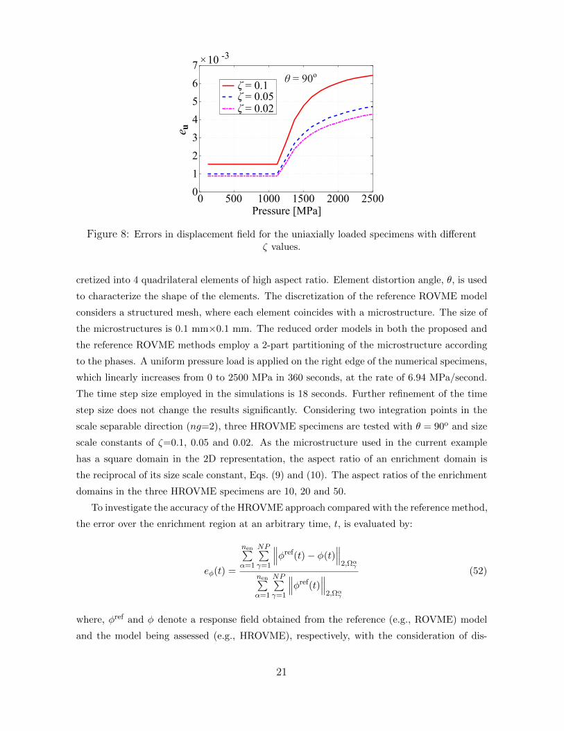
Figure 8: Errors in displacement field for the uniaxially loaded specimens with differentζ values.

cretized into 4 quadrilateral elements of high aspect ratio. Element distortion angle, θ, is used

to characterize the shape of the elements. The discretization of the reference ROVME model

considers a structured mesh, where each element coincides with a microstructure. The size of

the microstructures is 0.1 mm×0.1 mm. The reduced order models in both the proposed and

the reference ROVME methods employ a 2-part partitioning of the microstructure according

to the phases. A uniform pressure load is applied on the right edge of the numerical specimens,

which linearly increases from 0 to 2500 MPa in 360 seconds, at the rate of 6.94 MPa/second.

The time step size employed in the simulations is 18 seconds. Further refinement of the time

step size does not change the results significantly. Considering two integration points in the

scale separable direction (ng=2), three HROVME specimens are tested with θ = 90o and size

scale constants of ζ=0.1, 0.05 and 0.02. As the microstructure used in the current example

has a square domain in the 2D representation, the aspect ratio of an enrichment domain is

the reciprocal of its size scale constant, Eqs. (9) and (10). The aspect ratios of the enrichment

domains in the three HROVME specimens are 10, 20 and 50.

To investigate the accuracy of the HROVME approach compared with the reference method,

the error over the enrichment region at an arbitrary time, t, is evaluated by:

eφ(t) =

nen∑α=1

NP∑γ=1

∥∥∥φref(t)− φ(t)∥∥∥

2,Ωαγ

nen∑α=1

NP∑γ=1

∥∥∥φref(t)∥∥∥

2,Ωαγ

(52)

where, φref and φ denote a response field obtained from the reference (e.g., ROVME) model

and the model being assessed (e.g., HROVME), respectively, with the consideration of dis-

21

0 500 1000 1500 2000 2500Pressure [MPa]

0

0.02

0.04

0.06

0.08

0 500 1000 1500 2000 2500Pressure [MPa]

0

0.002

0.004

0.006

0.008

0.01

(a) (b)

ueue

θ = 90 o θ = 60 o θ = 45 o θ = 30 o

ζ = 0.1 θ = 90 o θ = 60 o θ = 45 o θ = 30 o

ζ = 0.02

Figure 9: Errors in displacement field for the uniaxially loaded specimens with differentθ and: (a) ζ=0.1; and (b) ζ=0.02.

cretization discrepancies. ‖ · ‖2,Ωαγ is the discrete L2 norm of the response field computed over

Ωαγ . Considering the ROVME model as the reference, the error in displacement field of the

proposed model is presented in Fig. 8 as a function of the applied pressure amplitude and

ζ. The accuracy of the proposed approach increases with decreasing ζ. This result agrees

with the fundamental property that the hybrid integration scheme is weakly convergent to the

reference approach at the limit ζ → 0. High accuracy is achieved for the simulations with less

than 1% maximum error. For each of the specimen, the error remains constant in the elastic

state (before pressure reaches 1250 MPa) and starts to accumulate at the onset of the inelastic

deformation. Compared with the reference simulations, the computational time improvement

of the proposed method is 6.43 times for ζ = 0.1, 9.54 times for ζ = 0.05 and 23.28 times for

ζ = 0.02.

HROVME simulations with various distortion angles, θ, are also performed. When θ=90o,

the specimen is discretized into four rectangular, undistorted, enrichment domains, while θ 6=90o implies distortion, with lower values indicating more significant distortion of the enrichment

domains. Comparing with the ROVME method, Figure 9 presents the displacement errors of

the proposed method as functions of the applied pressure amplitude, distortion and ζ. The

plots indicate accuracy degradation as the angle, θ, decreases. The discretization with lower ζ

is less sensitive to distortion induced accuracy degradation. The distortion effect is relatively

small when ζ/tanθ ≤ 0.03.

Remark 2. The current example demonstrates the accuracy of the HROVME method com-

pared to the ROVME method as the reference. The accuracy characteristics of the ROVME

approach have been demonstrated in Refs. [49, 50]. We further demonstrate the accuracy of

HROVME against the direct finite element analysis, which considers direct resolution of the

microstructure throughout the problem domain. Under the strain controlled tensile load which

22

0 0.01 0.02 0.03 0.04 0.05Strain

0

0.02

0.04

0.06

0.08

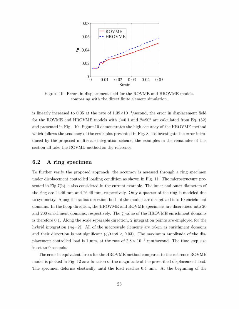
ROVMEHROVME

ue

Figure 10: Errors in displacement field for the ROVME and HROVME models,comparing with the direct finite element simulation.

is linearly increased to 0.05 at the rate of 1.39×10−4/second, the error in displacement field

for the ROVME and HROVME models with ζ=0.1 and θ=90o are calculated from Eq. (52)

and presented in Fig. 10. Figure 10 demonstrates the high accuracy of the HROVME method

which follows the tendency of the error plot presented in Fig. 8. To investigate the error intro-

duced by the proposed multiscale integration scheme, the examples in the remainder of this

section all take the ROVME method as the reference.

6.2 A ring specimen

To further verify the proposed approach, the accuracy is assessed through a ring specimen

under displacement controlled loading condition as shown in Fig. 11. The microstructure pre-

sented in Fig.7(b) is also considered in the current example. The inner and outer diameters of

the ring are 24.46 mm and 26.46 mm, respectively. Only a quarter of the ring is modeled due

to symmetry. Along the radius direction, both of the models are discretized into 10 enrichment

domains. In the hoop direction, the HROVME and ROVME specimens are discretized into 20

and 200 enrichment domains, respectively. The ζ value of the HROVME enrichment domains

is therefore 0.1. Along the scale separable direction, 2 integration points are employed for the

hybrid integration (ng=2). All of the macroscale elements are taken as enrichment domains

and their distortion is not significant (ζ/tanθ < 0.03). The maximum amplitude of the dis-

placement controlled load is 1 mm, at the rate of 2.8 × 10−3 mm/second. The time step size

is set to 9 seconds.

The error in equivalent stress for the HROVME method compared to the reference ROVME

model is plotted in Fig. 12 as a function of the magnitude of the prescribed displacement load.

The specimen deforms elastically until the load reaches 0.4 mm. At the beginning of the

23

uu

(a)

xz

12.23 mm13.23 mm

(b)

12.23 mm13.23 mm

xz

Figure 11: Model sketch and discretization of the ring specimen: (a) the HROVMEmacroscale model; and (b) the ROVME macroscale model.

0 0.25 0.5 0.75 1.0Displacement load [mm]

0.07

0.075

0.08

0.085

0.09

0.095

0.1

σe

Figure 12: Error in equivalent stress for the ring specimen.

24

(a)

P

P

x

z

20 mm 1 mm

(b)20 mm

1 mmx

z

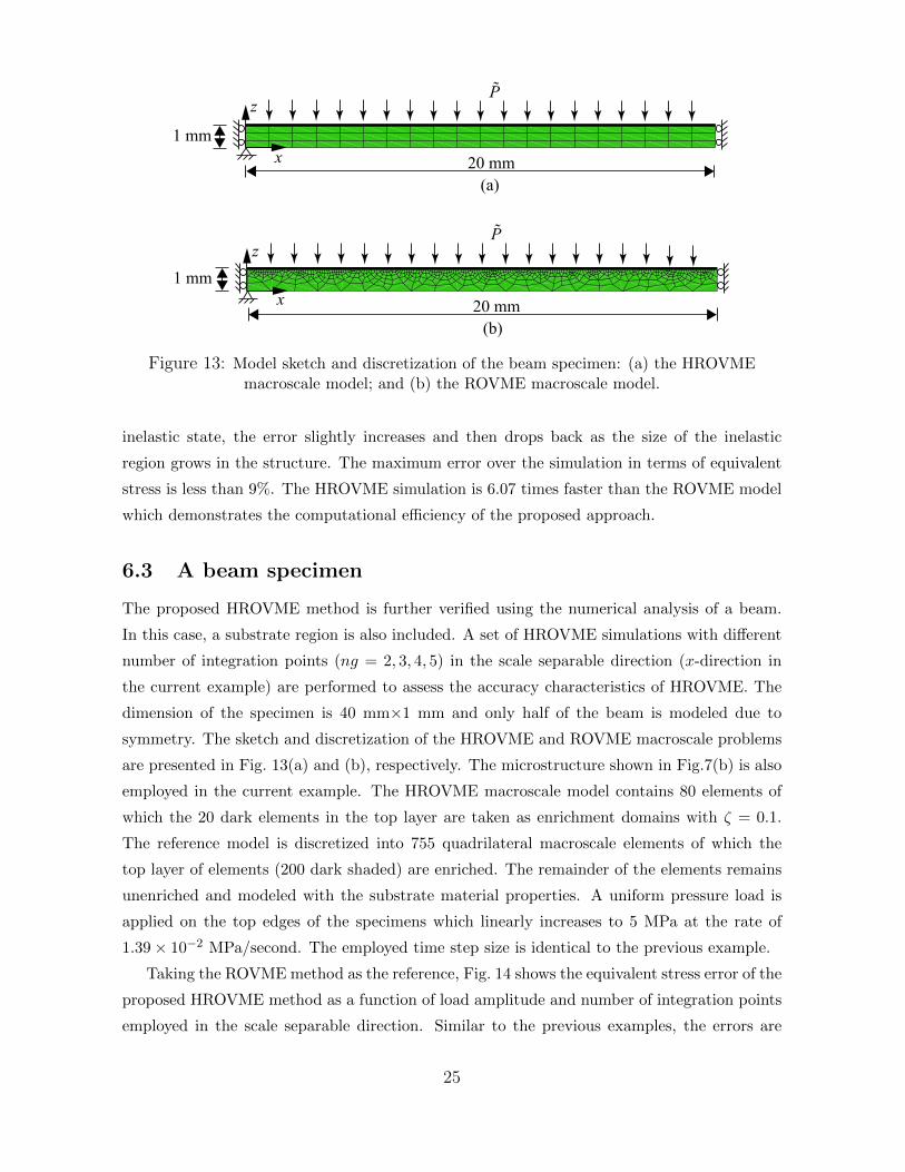
Figure 13: Model sketch and discretization of the beam specimen: (a) the HROVMEmacroscale model; and (b) the ROVME macroscale model.

inelastic state, the error slightly increases and then drops back as the size of the inelastic

region grows in the structure. The maximum error over the simulation in terms of equivalent

stress is less than 9%. The HROVME simulation is 6.07 times faster than the ROVME model

which demonstrates the computational efficiency of the proposed approach.

6.3 A beam specimen

The proposed HROVME method is further verified using the numerical analysis of a beam.

In this case, a substrate region is also included. A set of HROVME simulations with different

number of integration points (ng = 2, 3, 4, 5) in the scale separable direction (x-direction in

the current example) are performed to assess the accuracy characteristics of HROVME. The

dimension of the specimen is 40 mm×1 mm and only half of the beam is modeled due to

symmetry. The sketch and discretization of the HROVME and ROVME macroscale problems

are presented in Fig. 13(a) and (b), respectively. The microstructure shown in Fig.7(b) is also

employed in the current example. The HROVME macroscale model contains 80 elements of

which the 20 dark elements in the top layer are taken as enrichment domains with ζ = 0.1.

The reference model is discretized into 755 quadrilateral macroscale elements of which the

top layer of elements (200 dark shaded) are enriched. The remainder of the elements remains

unenriched and modeled with the substrate material properties. A uniform pressure load is

applied on the top edges of the specimens which linearly increases to 5 MPa at the rate of

1.39× 10−2 MPa/second. The employed time step size is identical to the previous example.

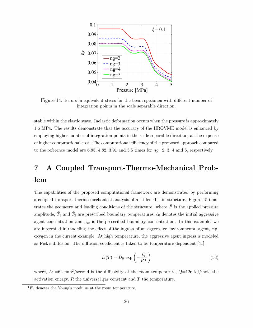
Taking the ROVME method as the reference, Fig. 14 shows the equivalent stress error of the

proposed HROVME method as a function of load amplitude and number of integration points

employed in the scale separable direction. Similar to the previous examples, the errors are

25

σePressure [MPa]

0.04

0.05

0.06

0.07

0.08

0.09

0.1

0 1 2 3 4 5

ng=2 ng=3 ng=4 ng=5

ζ = 0.1

Figure 14: Errors in equivalent stress for the beam specimen with different number ofintegration points in the scale separable direction.

stable within the elastic state. Inelastic deformation occurs when the pressure is approximately

1.6 MPa. The results demonstrate that the accuracy of the HROVME model is enhanced by

employing higher number of integration points in the scale separable direction, at the expense

of higher computational cost. The computational efficiency of the proposed approach compared

to the reference model are 6.95, 4.82, 3.91 and 3.5 times for ng=2, 3, 4 and 5, respectively.

7 A Coupled Transport-Thermo-Mechanical Prob-

lem

The capabilities of the proposed computational framework are demonstrated by performing

a coupled transport-thermo-mechanical analysis of a stiffened skin structure. Figure 15 illus-

trates the geometry and loading conditions of the structure. where P is the applied pressure

amplitude, T1 and T2 are prescribed boundary temperatures, c0 denotes the initial aggressive

agent concentration and c∞ is the prescribed boundary concentration. In this example, we

are interested in modeling the effect of the ingress of an aggressive environmental agent, e.g.

oxygen in the current example. At high temperature, the aggressive agent ingress is modeled

as Fick’s diffusion. The diffusion coefficient is taken to be temperature dependent [41]:

D(T ) = D0 exp

(− Q

RT

)(53)

where, D0=62 mm2/second is the diffusivity at the room temperature, Q=126 kJ/mole the

activation energy, R the universal gas constant and T the temperature.

1E0 denotes the Young’s modulus at the room temperature.

26

1808454

40

66

3

3

33

P

T1˜

c∞=0.05 c0=0.0015

T2˜

(a)

(b)

x

z

Figure 15: Model sketch of the stiffened panel specimen: (a) geometry in mm; and (b)loading conditions.

Table 3: Materials parameters for the transport-thermo-mechanical problem.

Material type E0 [GPa] 1 ν A [MPa] B [MPa] mPhase I 130 0.32 600 1000 0.85Phase II 107 0.32 350 250 0.85Substrate 120.8 0.32 500 700 0.85

Material type n F [MPa] γ[MPa/second] q αT [1/oC]Phase I 0.900 110 20 1.0 7.3×10−6

Phase II 0.975 110 20 1.0 8.3×10−6

Substrate 0.930 110 20 1.0 7.7×10−6

27

0 0.02 0.04 0.06 0.08Strain

0200400600800

100012001400

Stre

ss [M

Pa]

0 0.02 0.04 0.06 0.08Strain

0 0.02 0.04 0.06 0.08 0.1Strain

T=23 C, c=0.0015;o T=400 C, c=0.0015;o T=23 C, c=0.05;o T=400 C, c=0.05o

(a) (b) (c)

Figure 16: Constitutive response of the constituent materials at various temperature andaggressive agent concentration: (a) phase I; (b) phase II; and (c) substrate material.

In the context of small deformation theory, the mechanical material behavior is taken to

be elasto-viscoplastic. The temperature effect on the mechanical behavior of the constituent

materials is modeled through temperature dependent elastic moduli, yielding and the thermal

expansion which are considered following the algorithms in Ref. [50]. The viscoplastic harden-

ing of the constituent materials is taken to be a function of the aggressive agent concentration

and temperature through the modified Johnson-Cook model as [41]:

σy = [A+B(εvp)n + Fc] [1− (T ∗)m] (54)

where, A, B, F , m and n are material parameters; c the aggressive agent concentrate and T ∗

the non-dimensional temperature:

T ∗ =T − Troom

Tmelt − Troom(55)

in which, Troom and Tmelt are the room and melting temperatures, respectively. A two-phase

microstructure is considered for the material. The material properties of the constituent

materials are listed in Table 3. The Young’s moduli of the materials linearly vary as a function

of temperature with 0.0381 GPa/oC, 0.0314 GPa/oC and 0.0354 GPa/oC for phases I and II,

and the substrate materials. The properties of the substrate material are obtained through

mixture theory. At 0.056/second of strain loading rate, the constitutive responses of the

constituent materials under various temperature and concentration conditions are plotted in

Fig. 16.

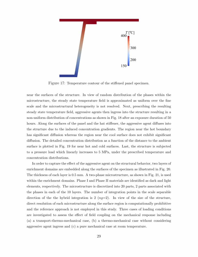
First, the top and bottom surfaces of the structure are exposed to 400oC and 150oC, which

results in a non-uniform temperature distribution over the structure as shown in Fig. 17. In

this analysis, the temperature distribution is obtained from a direct finite element simulation

of the classical steady state heat conduction (i.e., Ficks law) using a very fine discretization

28

400T [ C]o

150200

300

Figure 17: Temperature contour of the stiffened panel specimen.

near the surfaces of the structure. In view of random distribution of the phases within the

microstructure, the steady state temperature field is approximated as uniform over the fine

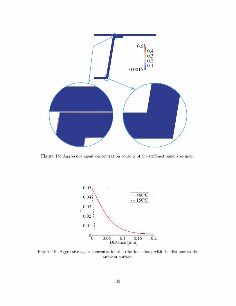
scale and the microstructural heterogeneity is not resolved. Next, prescribing the resulting

steady state temperature field, aggressive agents then ingress into the structure resulting in a

non-uniform distribution of concentrations as shown in Fig. 18 after an exposure duration of 50

hours. Along the surfaces of the panel and the hat stiffener, the aggressive agent diffuses into

the structure due to the induced concentration gradients. The region near the hot boundary

has significant diffusion whereas the region near the cool surface does not exhibit significant

diffusion. The detailed concentration distribution as a function of the distance to the ambient

surface is plotted in Fig. 19 for near hot and cold surfaces. Last, the structure is subjected

to a pressure load which linearly increases to 5 MPa, under the prescribed temperature and

concentration distributions.

In order to capture the effect of the aggressive agent on the structural behavior, two layers of

enrichment domains are embedded along the surfaces of the specimen as illustrated in Fig. 20.

The thickness of each layer is 0.5 mm. A two-phase microstructure, as shown in Fig. 21, is used

within the enrichment domains. Phase I and Phase II materials are identified as dark and light

elements, respectively. The microstructure is discretized into 20 parts, 2 parts associated with

the phases in each of the 10 layers. The number of integration points in the scale separable

direction of the the hybrid integration is 2 (ng=2). In view of the size of the structure,

direct resolution of each microstructure along the surface region is computationally prohibitive

and the reference approach is not employed in this study. Three cases of loading conditions

are investigated to assess the effect of field coupling on the mechanical response including

(a) a transport-thermo-mechanical case, (b) a thermo-mechanical case without considering

aggressive agent ingress and (c) a pure mechanical case at room temperature.

29

0.5

0.00150.10.20.30.4

c

Figure 18: Aggressive agent concentration contour of the stiffened panel specimen.

0 0.05 0.15 0.2

c

0

0.01

0.02

0.03

0.04

0.05

Distance [mm]0.1

400oC150oC

Figure 19: Aggressive agent concentration distributions along with the distance to theambient surface.

30

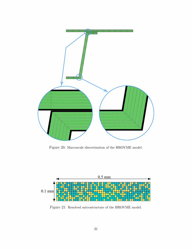
Figure 20: Macroscale discretization of the HROVME model.

0.5 mm

0.1 mm

Figure 21: Resolved microstructure of the HROVME model.

31

Pressure [MPa]

-8

-6

-4

-2

0

Def

lect

ion

[mm

]

0 1 2 3 4 5

Transport-thermo-mechanicalThermo-mechanicalMechanical

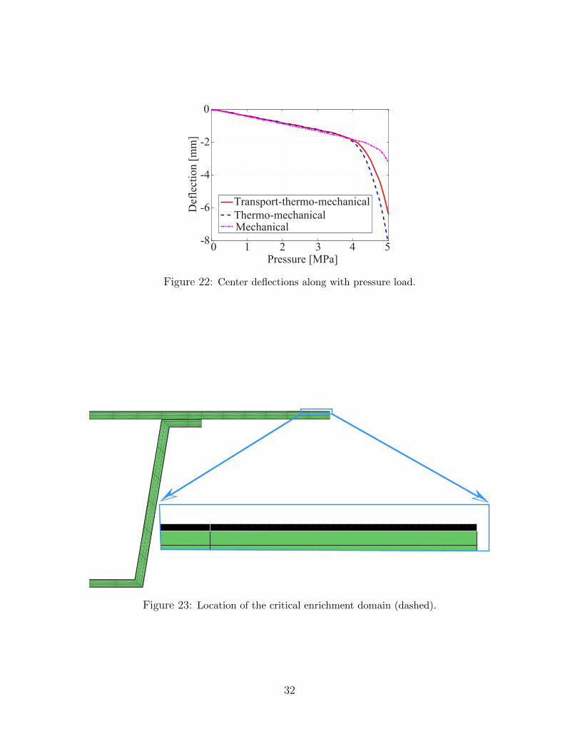
Figure 22: Center deflections along with pressure load.

Figure 23: Location of the critical enrichment domain (dashed).

32

(a)

(b)

(c)

400600800100012001400

σ[MPa]

Figure 24: Stress countours of the critical microstructure for specimen subjected to: (a)transport-thermo-mechanical loads; (b) thermo-mechanical loads; and (c) only

mechanical load.

Figure 22 shows the deflection of the center of the stiffened panel for the three cases as a

function of applied load. When contrasting cases (b) and (c), the presence of high temper-

ature clearly reduces the overall stiffness of the structure and induces inelastic deformations

with notably larger magnitudes. In the presence of aggressive agent ingress, case (a), the

specimen exhibits a clearly stiffer response than case (b). We note that although diffusion

affects the structure along a narrow surface region, the deflection change in the inelastic stage

is significant. Maximum stress is contained by the critical enrichment domain right next to

the top center point of the panel. The location of the critical enrichment domain in the

structure is identified as the dashed element which is shown in Fig. 23. The local equivalent

stress distribution within the microstructure of the critical enrichment domain is presented in

Fig. 24 for all three simulations. For plotting purposes, the microstructural stress distributions

are reconstructed over the microstructure during post-processing. The plots indicate uniform

stress distribution over the parts of the microstructure consistent with the reduced order ap-

proximation. The transport-thermo-mechanical specimen, case (a), demonstrates significantly

higher equivalent stress due to the ingress effect and high temperature induced expansion.

More importantly, the HROVME method has the capability of capturing the stress gradient

induced by the aggressive agent concentration variation across the thickness of the enrichment

domain, as shown in Fig. 24(a). In the absence of aggressive agent, the local responses of

the thermo-mechanical and mechanical simulations (Figs. 24(b) and (c)) exhibit more uniform

stress distributions within the microstructure.

33

8 Conclusions

This manuscript presented a new hybrid multiscale integration scheme for directionally scale

separable multiscale problems. The proposed approach is particularly suitable for structural

problems, where surface degradation and embrittlement effects are critical to the overall re-

sponse. The proposed hybrid multiscale integration algorithm was applied to arrive at a

reduced order multiscale variational multiscale enrichment model (HROVME), which demon-

strates significant computational efficiency and reasonable accuracy. The investigations in the

current manuscript are limited to the viscoplastic behavior within the material constituents.

Surface degradation problems are typically associated with early onset of microcracking that

changes the stress distributions within the surface region affected by the aggressive agent.

Future investigations must therefore focus on the extension of the proposed multiscaling algo-

rithm to account for the nucleation and growth of microcracks within the enrichment domains.

This poses significant challenges in terms of the enforcement of appropriate boundary condi-

tions for the microscale problem, as well as the model order reduction of a microstructure that

evolves as a function of the load state.

9 Acknowledgements

The authors gratefully acknowledge the research funding from the Air Force Office of Scientific

Research Multi-Scale Structural Mechanics and Prognosis Program (Grant No: FA9550-13-1-

0104. Program Manager: Dr. Jaimie Tiley). We also acknowledge the technical cooperation

of the Structural Sciences Center at the Air Force Research Laboratory.

References

[1] T. Arbogast. Implementation of a locally conservative numerical subgrid upscaling scheme

for two-phase Darcy flow. Comput. GeoSci., 6:453–481, 2002.

[2] T. Arbogast. Analysis of a two-scale, locally conservative subgrid upscaling for elliptic

problems. SIAM J. on Numer. Anal., 42:576–598, 2004.

[3] I. Babuska. Homogenization and application: mathematical and computational prob-

lems, in: B. Hubbard (Ed.), Numerical Solution of Partial Differential Equations - III.

SYNSPADE, New York, 1975.

[4] Y. A. Bahei-El-Din, A. M. Rajendran, and M. A. Zikry. A micromechanical model for

34

damage progression in woven composite systems. Int. J. Solids Structures, 41:2307–2330,

2004.

[5] T. Belytschko, J. S.-J. Ong, W. K. Liu, and J. M. Kennedy. Hourglass control in linear

and nonlinear problems. Comput. Methods Appl. Mech. Engrg., 43:251–276, 1984.

[6] A. Bensoussan, J-L. Lions, and G. Papanicolau. Asymptotic Analysis for Periodic Struc-

tures. Elsevier, 1978.

[7] D. Bettge, B. Gunther, W. Wedell, P.D. Portella, J. Hemptenmacher, P.W.M. Peters, and

B. Skrotzki. Mechanical behavior and fatigue damage of a titanium matrix composite

reinforced with continuous SiC fibers. Mater. Sci. Eng., A, 452-453:536–544, 2007.

[8] S. Bhattacharjee and K. Matous. A nonlinear manifold based reduced order model for

multiscale analysis of heterogeneous hyperelastic materials. J. Comput. Phys., 313:635–

653, 2016.

[9] F. Bignonnet, K. Sab, L. Dormieux, S. Brisard, and A. Bisson. Macroscopically consistent

non-local modeling of heterogeneous media. Comput. Methods Appl. Mech. Engrg., 278:

218–238, 2014.

[10] F. Brezzi, L. P. Franca, T. J. R. Hughes, and A. Russo. b =∫g. Comput. Methods Appl.

Mech. Engrg., 145:329–339, 1997.

[11] N. Carrere, D. Boivin, R. Valle, and A. Vassel. Local texture measurements in a SiC/Ti

composite manufactured by the foil-fiber-foil. Scripta Mater., 44:867–872, 2001.

[12] J. L. Chaboche, S. Kruch, J. F. Maire, and T. Pottier. Towards a micromechanics based

inelastic and damage modeling of composites. Int. J. Plasticity, 17:411–439, 2001.

[13] D. Cioranescu and P. Donato. An Introduction to Homogenization. Oxford University

Press, 1999.

[14] R. D. Cook, D. S. Malkus, M. E. Plesha, and R. J. Witt. Concepts and Applications of

Finite Element Analysis, 4th Edition. John Wiley & Sons. Inc., 2002.

[15] C. A. Duarte and D. J. Kim. Analysis and applications of a generalized finite element

method with global–local enrichment functions. Comput. Methods Appl. Mech. Engrg.,

197:487–504, 2008.

[16] G. J. Dvorak. Transformation field analysis of inelastic composite materials. Proc. R.

Soc. Lond. A, 437:311–327, 1992.

35

[17] W. E, P. Ming, and P. Zhang. Analysis of the heterogeneous multiscale method for elliptic

homogenization problems. J. Am. Math. Soc., 18:121–156, 2004.

[18] Y. Efendiev, J. Galvis, and T. Hou. Generalized multiscale finite element methods. J.

Comput. Phys., 251:116–135, 2013.

[19] A. G. Evans, F.W. Zok, R. M. McMeeking, and Z. Z. Du. Models of high temperature,

environmentally assisted embrittlement in ceramic matrix composites. J. Am. Ceram.

Soc., 79:2345–2352, 1996.

[20] J. Fish. The s-version of the finite element method. Computers & Structures, 43:539–547,

1992.

[21] J. Fish and S. Markolefas. Adaptive global-local refinement strategy based on the interior

error estimates of the h-method. Int. J. Numer. Meth. Engng., 37:827–838, 1994.

[22] L. Gendre, O. Allix, P. Gosselet, and F. Comte. Non-intrusive and exact global/local

techniques for structural problems with local plasticity. Comput. Mech., 44:233–245,

2009.

[23] J. M. Guedes and N. Kikuchi. Preprocessing and postprocessing for materials based on the

homogenization method with adaptive finite element methods. Comput. Methods Appl.

Mech. Engrg., 83:143–198, 1990.

[24] T. Y. Hou and X. Wu. A multiscale finite element method for elliptic problems in com-

posite materials and porous media. J. Comput. Phys., 134:169–189, 1997.

[25] T. J. R. Hughes. Multiscale phenomena: Green’s functions, the Dirichlet-to-Neumann

formulation, subgrid scale models, bubbles and the origins of stabilized methods. Comput.

Methods Appl. Mech. Engrg., 127:387–401, 1995.

[26] T. J. R. Hughes. The Finite Element Method: Linear Static and Dynamic Finite Element

Analysis. Prentice-Hall, Inc. Englewood Cliffs, N. J., 2000.

[27] T. J. R. Hughes, G. R. Feijoo, and J. B. Quincy. The variational multiscale method - a

paradigm for computational mechanics. Comput. Methods Appl. Mech. Engrg., 166:3–24,

1998.

[28] O. P. Jacquotte and J. T. Oden. Analysis of hourglass instabilities and control in un-

derintegrated finite element methods. Comput. Methods Appl. Mech. Engrg., 44:339–363,

1984.

36

[29] A. Levy and Y.-F. Man. Surface degradation of ductile metal in elevated temperature

gas-particle streams. Wear, 111:173–186, 1986.

[30] O. Lloberas-Valls, D. J. Rixen, A. Simone, and L. J. Sluys. Domain decomposition

techniques for the efficient modeling of brittle heterogeneous materials. Comput. Methods

Appl. Mech. Engrg., 200:1577–1590, 2011.

[31] K. M. Mao and C. T. Sun. A refined global-local finite element analysis method. Int. J.

Numer. Meth. Engng., 32:29–43, 1991.

[32] J.C. Michel and P. Suquet. Computational analysis of nonlinear composite structures

using the nonuniform transformation field analysis. Comput. Methods Appl. Mech. Engrg.,

193:5477–5502, 2004.

[33] H. Moulinec and P. Suquet. A numerical method for computing the overall response of

nonlinear composites with complex microstructure. Comput. Methods Appl. Mech. Engrg.,

157:69–94, 1998.

[34] A. K. Noor. Global-local methodologies and their application to nonlinear analysis. Finite

Elements Anal. Des., 2:333–346, 1986.

[35] P. O’ Hara, C. A. Duarte, T. Eason, and J. Garzon. Efficient analysis of transient heat

transfer problems exhibiting sharp thermal gradients. Comput. Mech., 51:743–764, 2013.

[36] J. Oliver, M. Caicedo, A.E. Huespe, J.A. Hernandez, and E. Roubin. Reduced order

modeling strategies for computational multiscale fracture. Comput. Meth. Appl. Mech.

Engng,, 313:560–595, 2017.

[37] R. A. Oriani. Hydrogen embrittlement of steels. Ann. Rev. Mater. Sci., 8:327–357, 1978.

[38] C. Oskay. Variational multiscale enrichment for modeling coupled mechano-diffusion prob-

lems. Int. J. Numer. Meth. Engng., 89:686–705, 2012.

[39] C. Oskay. Variational multiscale enrichment method with mixed boundary conditions for

modeling diffusion and deformation problems. Comput. Methods Appl. Mech. Engrg., 264:

178–190, 2013.

[40] C. Oskay and J. Fish. Eigendeformation-based reduced order homogenization for failure

analysis of heterogeneous materials. Comput. Methods Appl. Mech. Engrg., 196:1216–

1243, 2007.

[41] C. Oskay and M. Haney. Computational modeling of titanium structures subjected to

thermo-chemo-mechanical environment. Int. J. Solids Struct., 47:3341–3351, 2010.

37

[42] P. A. Sparks and C. Oskay. Identification of optimal reduced order computational models

for failure of heterogeneous materials. Int. J. Mult. Comp. Eng., 11:185–200, 2013.

[43] P. A. Sparks and C. Oskay. The method of failure paths for reduced-order computational

homogenization. Int. J. Mult. Comp. Eng., 14:515–534, 2016.

[44] S. P. Walker and B. J. Sullivan. Sharp refractory composite leading edges on hypersonic

vehicles. AIAA 20036915, Proceedings of the 12th AIAA International Space Planes and

Hypersonic Systems and Technologies, 1519 December 2003, Norfolk, VA., 2003.

[45] R.G. Wellman and J.R. Nicholls. High temperature erosion-oxidation mechanisms, maps

and models. Wear, 256:907917, 2004.

[46] H. Yan and C. Oskay. A viscoelastic-viscoplastic model of titanium structures subjected

to thermo-chemo-mechanical environment. Int. J. Solids Struct., 56-57:29–42, 2015.

[47] J. Yvonnet and Q.-C. He. The reduced model multiscale method (R3M) for the non-linear

homogenization of hyperelastic media at finite strains. J. Comput. Phys., 223:341–368,

2007.

[48] S. Zhang and C. Oskay. Variational multiscale enrichment method with mixed boundary

conditions for elasto-viscoplastic problems. Comput. Mech., 55:771–787, 2015.

[49] S. Zhang and C. Oskay. Reduced order variational multiscale enrichment method for

elasto-viscoplastic problems. Comput. Methods Appl. Mech. Engrg., 300:199–224, 2016.

[50] S. Zhang and C. Oskay. Reduced order variational multiscale enrichment method for

thermo-mechanical problems. Comput. Mech., 59:887–907, 2017.

38

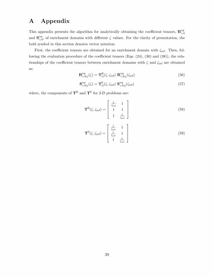
A Appendix

This appendix presents the algorithm for analytically obtaining the coefficient tensors, BαgγA

and SαgγA, of enrichment domains with different ζ values. For the clarity of presentation, the

bold symbol in this section denotes vector notation.

First, the coefficient tensors are obtained for an enrichment domain with ζref. Then, fol-

lowing the evaluation procedure of the coefficient tensors (Eqs. (24), (30) and (38)), the rela-

tionships of the coefficient tensors between enrichment domains with ζ and ζref are obtained

as:

BαgγAij(ζ) = TB

ij(ζ, ζref) BαgγAij(ζref) (56)

SαgγAij(ζ) = TSij(ζ, ζref) SαgγAij(ζref) (57)

where, the components of TB and TS for 2-D problems are:

TB(ζ, ζref) =

ζζref

1

1 1

1 ζζref

(58)

TS(ζ, ζref) =

ζζref

1ζζref

1

1 ζζref

(59)

39