hybrid modelling and optimal control of a multiproduct batch plant
TRANSCRIPT

Control Engineering Practice 12 (2004) 1127–1137
ARTICLE IN PRESS
*Correspondi
631.
E-mail addre
0967-0661/$ - see
doi:10.1016/j.con
Hybrid modelling and optimal control of a Multiproduct Batch Plant
Bo$stjan PotoWnika,*, Alberto Bemporadb, Fabio Danilo Torrisic,Ga$sper Mu$siWa, Borut ZupanWiWa
aLaboratory of Modelling, Simulation and Control, Faculty of Electrical Engineering, University of Ljubljana, Trma$ska 25, SI-1000 Ljubljana, SloveniabDip. Ingegneria dell’Informazione, Universit "a di Siena, Via Roma 56, I-53100 Siena, Italy
cAutomatic Control Laboratory, ETH – Swiss Federal Institute of Technology, CH-8092 Z .urich, Switzerland
Received 14 October 2002; accepted 28 November 2003
Abstract
This paper addresses the problem of optimally selecting the production plan for a Multiproduct Batch Plant. The proposed
approach can also be applied to a broader class of optimal control problems for systems with discrete inputs. The plant is modelled
as a Discrete Hybrid Automaton (DHA) using the high level modelling language, HYbrid System DEscription Language
(HYSDEL), which allows conversion of the DHA model into an Mixed Logical Dynamical (MLD) model. The solution algorithm,
which takes into account a model of a hybrid system described as an MLD system, is based on reachability analysis ideas. The
algorithm abstracts the behaviour of the hybrid system into a ‘‘tree of evolution’’, where nodes of the tree represent reachable states
of the system, and branches connect two nodes if a transition exists between the corresponding states. To each node a cost function
value is associated and, based on this value, the tree exploration is driven, searching for the optimal control profile.
r 2004 Elsevier Ltd. All rights reserved.
Keywords: Hybrid systems; Modelling; Optimal control; Reachability analysis; Branch-and-bound methods
1. Introduction
Hybrid systems are dynamic systems that involve theinteraction of continuous dynamics (modelled as differ-ential or difference equations) and discrete dynamics(modelled by finite state machines (FSM)). Hybridsystems have been a topic of intense research activityin recent years, primarily because of their potentialimportance in applications, e.g. the process industry.Hybrid models are important to a number of problemsin system analysis, such as the computation oftrajectories, control, stability and safety analysis, etc.Mathematical models represent the basis of any
system analysis and design such as simulation, control,verification, etc. The model should not be too compli-cated, in order to efficiently define the system behaviour,and not too simple, otherwise it is too far from thebehaviour of the real process. We model a hybrid systemas a discrete hybrid automaton (DHA) using themodelling language HYbrid System DEscription Lan-guage (HYSDEL) (Torrisi & Bemporad, 2002). Using
ng author. Tel.: +386-1-4768-764; fax: +386-1-4264-
ss: [email protected] (B. PotoWnik).
front matter r 2004 Elsevier Ltd. All rights reserved.
engprac.2003.11.010
an appropriate compiler, a DHA model can betranslated to different modelling frameworks, such asmixed logical dynamical (MLD), piecewise affine (PWA),linear complementarity (LC), extended linear complemen-
tarity (ELC) or max-min-plus-scaling (MMPS) systems(Torrisi & Bemporad, 2002; Heemels, De Schutter, &Bemporad, 2001). In this paper the MLD modellingframework presented in Bemporad and Morari (1999)will be adopted, as it is mostly suitable for solvingoptimal control problems. Moreover, it enables theincorporation of additional working constraints andheuristics that usually appear in industry. Indeed,several control procedures based on the MLD descrip-tion of a process have been proposed in the literature.A model predictive control technique is prese-nted in Bemporad and Morari (1999) which is able tostabilize an MLD system on a desired referencetrajectory, where on-line optimisation procedures aresolved through mixed integer quadratic programming
(MIQP) (Bemporad & Mignone, 2000). A verificationapproach for hybrid systems is presented in Bemporad,Giovanerdi, and Torrisi (2001).Optimal control laws for hybrid systems have been
widely investigated in recent years, and many results canbe found in control engineering literature. Optimal

ARTICLE IN PRESSB. Potocnik et al. / Control Engineering Practice 12 (2004) 1127–11371128
control of hybrid systems in manufacturing is addressedin Antsaklis (2000), Cassandras, Pepyne, and Wardi(2001), and Gokbayrak and Cassandras (1999), wherethe authors combine time-driven and event-drivenmethodologies to solve optimal control problems. Analgorithm to optimise switching sequences for a class ofswitched linear problems is presented in Lincoln andRantzer (2001), where the algorithm searches forsolutions arbitrarily close to the optimal ones. A similarproblem is addressed in Barton, Banga, and Galan(2000), where the potential for numerical optimisationprocedures to make optimal sequencing decisions inhybrid dynamic systems is explored. A computationalapproach based on ideas from dynamic programmingand convex optimisation is presented in Hedlund andRantzer (1999). Piecewise linear quadratic optimalcontrol is addressed in Rantzer and Johansson (2000),where the use of piecewise quadratic cost functions isextended from a stability analysis of piecewise linearsystems. Optimal control based on reachability analysisand where the inputs of the system are continuous isaddressed in Bemporad et al. (2000). A similar idea ishere applied to hybrid systems with discrete inputs only.More precisely, in this paper we will address the timeoptimal control problem of processes with discreteinputs only. The solution to the problem is applied tothe Multiproduct Batch Plant example. The solution tothe time optimal problem for the example underconsideration can be considered as a schedulingproblem, as we try to compute the times at whichcertain decisions are taken. We will, rather, refer tooptimal control, as the proposed approach can also beused for the control of hybrid systems where it isdifficult to characterise the control problem as ascheduling problem.The paper is organised as follows. In Section 2 we
address the DHA and MLD modelling frameworks. Theproblem formulation and proposed solution are ad-dressed in Section 3. The proposed algorithm is appliedto the Multiproduct Batch Plant and is discussed inSection 4. The conclusions are given in Section 5.
2. DHA and MLD systems
In this section we introduce the modelling frameworkused for the modelling of a hybrid system. A hybridsystem is modelled as a DHA using the HYSDELmodelling language. Using an appropriate compiler,such a model can be translated into a MLD modellingframework that is used by the optimisation algorithm.DHA are formulated in discrete time and result from
the interconnection of a finite state machine (FSM),which provides the discrete part of the hybrid system,with a switched affine system (SAS), which provides thecontinuous part of the hybrid dynamics. The interaction
between the two is based on two connecting elements:the event generator (EG), which extracts logic signalsfrom the continuous part, and the mode selector (MS),which defines the mode (continuous dynamics) of theSAS based on logic variables (states, inputs and events)Torrisi and Bemporad, 2002. At this point we have tostress that we are dealing with a special case where thesystem includes only discrete inputs, i.e. continuousinputs are not present. Note that we will introducebelow a modified DHA system based on this fact. Themodified DHA system is shown in Fig. 1.A SAS without continuous inputs represents a
sampled continuous system that is described by thefollowing set of linear affine equations:
xrðk þ 1Þ ¼ AiðkÞxrðkÞ þ f iðkÞ;
yrðkÞ ¼ CiðkÞxrðkÞ þ giðkÞ; ð1Þ
where kAZX0 represents the independent variable (timestep) (ZX09f0; 1;yg is a set of non-negative integers),xrAXrDRnr is the continuous state vector, yrAYrDRpr
is the continuous output vector, fAi; f i;Ci; gigiAI is a setof matrices of suitable dimensions, and I is a set ofvariables that select the linear state update dynamics.An EG generates a logic signal according to the
satisfaction of linear affine constraints deðkÞ ¼fH ðxrðkÞ; kÞ; where fH : Rnr � ZX0-DDf0; 1gne is avector of descriptive functions of a linear hyperplane.The relation fH for time events is modelled as ½di
eðkÞ ¼ 12½kTsXti; where Ts is the sampling time, while forthreshold events it is modelled as ½di
eðkÞ ¼ 12½aT
i xrðkÞpci; and where ai and ci represent theparameters of a linear hyperplane. di
e denotes the ithcomponent of a vector deðkÞ:A FSM is a discrete dynamic process that evolves
according to a logic state update function xbðk þ 1Þ ¼fBðxbðkÞ; ubðkÞ; deðkÞÞ; where xbAXbDf0; 1gnb is theBoolean state, ubAUbDf0; 1gmb is the Boolean input,deðkÞ is the input coming from the EG, and fB : Xb �Ub �D-Xb is a deterministic logic function. A FSMmay also have associated Boolean output ybðkÞ ¼gBðxbðkÞ; ubðkÞ; deðkÞÞ; where ybAYbDf0; 1gpb :A MS selects the dynamic mode iðkÞ of the SAS using
Boolean function fM :Xb �Ub �D-I while consider-ing the Boolean states xbðkÞ; the Boolean inputs ubðkÞand the events deðkÞ: The output of this function iðkÞ ¼fMðxbðkÞ; ubðkÞ; deðkÞÞ is called the active mode.DHA models can be built by using the HYSDEL
modelling language, which was designed particularly forthis class of systems. The HYSDEL modelling languageallows the description of hybrid dynamics in textualform. Using an associated compiler this form can betranslated into MLD form (Bemporad & Morari, 1999).For a more detailed description of the syntax and thefunctionality of the HYSDEL modelling language andthe associated compiler (HYSDEL tool) the reader is

ARTICLE IN PRESS
EventGenerator
Mode Selector
SwitchedAffine ystemsS( )SAS
( )MS
z-1
Finite State Machine( )FSM
1
s
z-1
Clock
xr( + 1)k
i k( )
xb( )k
ub( )k
�e( )k
xb( )kxb( + 1)k
ub( )k
�e( )k ( )EG
1
&
...xr( )k
Fig. 1. A DHA without continuous inputs.
B. Potocnik et al. / Control Engineering Practice 12 (2004) 1127–1137 1129
referred to Torrisi and Bemporad (2002) and Torrisiet al. (2002).Once a DHA system is modelled by the HYSDEL
modelling language, the companion HYSDEL compilergenerates the equivalent MLD model of the form (2).The transformation of a DHA into an equivalent MLDform is presented in Torrisi and Bemporad (2002) andwill not be reported here due to space limitations. AnMLD system, restricted to discrete inputs only, isdescribed by the following relations:
xðk þ 1Þ ¼ AxðkÞ þ B1ubðkÞ þ B2dðkÞ þ B3zðkÞ; ð2aÞ
yðkÞ ¼ CxðkÞ þ D1ubðkÞ þ D2dðkÞ þ D3zðkÞ; ð2bÞ
E2dðkÞ þ E3zðkÞpE1ubðkÞ þ E4xðkÞ þ E5; ð2cÞ
where x ¼ ½xr; xb0ARnr � f0; 1gnb is a vector ofcontinuous and logic states, ubAf0; 1gmb are the logic(discrete) inputs, y ¼ ½yr; yb
0ARpr � f0; 1gpb the outputs,dAf0; 1grb ; zARrr auxiliary logic and continuousvariables, respectively, and A; B1; B2; B3; C; D1;D2; D3; E1;y;E5 are matrices of suitable dimensions.Inequalities (2c) can also contain additional constraintson the variables (states, inputs and auxiliary variables).This permits the inclusion of additional constraints andthe incorporation of heuristic rules into the model.Using the current state xðkÞ and input ubðkÞ; the time
evolution of (2) is determined by solving dðkÞ and zðkÞfrom (2c), and then updating xðk þ 1Þ and yðkÞ fromEqs. (2a) and (2b). The MLD system (2) is assumed tobe completely well-posed if, for a given state xðkÞ andinput ubðkÞ; inequalities (2c) have a unique solution for
dðkÞ and zðkÞ: A simple algorithm to test well-posednessis given in Bemporad and Morari (1999).
3. A class of optimal control problems
Optimal control amounts to finding the controlsequence Ukfin�1
0 ¼ fubð0Þ;y; ubðkfin � 1Þg which trans-fers the initial state x0 to the final state xfin in a finitetime T ¼ kfin � Ts ðTs is the sampling time) whileminimising a certain performance index. In this paperwe will tackle a class of time optimal control problemswhere the system can be influenced through discreteinputs only, i.e. ubðkÞAf0; 1gmb : A hybrid system will bemodelled as an MLD system due to its compact andpowerful description. An optimal control problem willbe solved by extending ideas described in Bemporadet al. (2000), where the optimal control of hybridsystems with continuous inputs using reachabilityanalysis is proposed.
3.1. Complexity of the problem
The solution to the posed optimal control problem isthe optimal control sequence Ukfin�1
0 ¼ fubð0Þ;y;ubðkÞ;y; ubðkfin � 1Þg; where ubðkÞ represents the dis-crete input to the system at step k: Due to the fact thatwe are dealing with a system with mb discrete inputsand no continuous inputs (ubðkÞAf0; 1gmb andUkfin�10 Af0; 1gmb�kfin ), there are 2mb�kfin possible combina-
tions for Ukfin�10 : Hence the optimisation problem is
NP-hard and the computational time required to solvethe problem grows exponentially with the problem size

ARTICLE IN PRESS
Fig. 2. Tree of evolution.
B. Potocnik et al. / Control Engineering Practice 12 (2004) 1127–11371130
ðan; for a > 1Þ; so that any enumeration method wouldbe impractical.
3.2. Optimisation based on reachability analysis
In general, not all the combinations of inputs arefeasible, due to the constraints (2c). One approach torule out infeasible inputs is to use reachability analysis.The idea for hybrid systems with continuous inputspresented in Bemporad et al. (2000) is adapted here tohybrid systems with discrete inputs.Using reachability analysis it is possible to determine
the admissible control sequences Ukfin�10 : As many of
them will be far away from the optimal one, it isreasonable to selectively propagate the search foradmissible control sequences. More precisely, thepropagation is driven in accordance with the value ofa cost function J that evaluates the efficiency of thepropagation. We will introduce below the basic parts ofthe algorithm, i.e. reachability analysis, the constructionof a tree of evolution, cost selection criteria and nodeselection criteria. The whole procedure is a kind ofbranch and bound strategy, namely by searching forreachable states we branch the evolution tree, and byremoving non-optimal ones we bound it.
3.2.1. Reachability analysis
Let xðkÞ be the state at step k: Reachability analysiscomputes all the reachable states xjðk þ 1Þ at the nextstep considering all possible discrete inputs ubðkÞ to thesystem and where jAf1; 2;yg is an index markingreachable states. If a system has mb discrete inputs, then2mb possible next states may exist. However, because ofthe operating constraints that are usually contained in asystem, only a smaller number of states can actually bereached. The reachable states xjðk þ 1Þ are computed byapplying the state xðkÞ and all possible inputs ubðkÞ atstep k to the MLD model (2) of a hybrid system.Reachable (feasible) states are actually defined by theinequalities (2c).
3.2.2. Tree of evolution
By exploiting the reachability analysis technique, weare able to abstract the possible evolution of the systemover a horizon of maximum kmax steps into a ‘‘tree ofevolution’’ (Bemporad et al., 2000) as shown in Fig. 2.The nodes of the tree represent reachable states, andbranches connect two nodes if a transition existsbetween corresponding states. Each branch has anassociated discrete input applied to the system causingthe transition. For a given root node V0; representingthe initial state x0; reachable states are computed andinserted into the tree as nodesVi; while the correspond-ing discrete inputs ui
bðkÞ are associated with thecorresponding branches connecting two nodes.iAf0; 1;yg represents the successive index of the nodes
and branches inserted into the tree. To each new nodeVi a cost value Ji is associated. The search for theoptimal control sequence is propagated from a newstarting node, whose selection is based on the associatedcost value Ji: As soon as a new starting node is selected,new reachable states are computed. The construction ofthe ‘‘tree of evolution’’ proceeds according to a depthfirst strategy until one of the following conditionsoccurs:
* the horizon limit of kmax steps has been reached* the final state has been reached ðxðkÞ ¼ xfinÞ* the value of the cost function at the current node isgreater than the current optimal one (JiXJopt; whereinitially Jopt ¼ N).
A node that satisfies one of the above conditions islabelled as explored. If a node satisfies the first or secondcondition, the associated value of the cost function Ji
becomes the current optimal one ðJopt ¼ JiÞ; thecorresponding step k indicates the number of stepsleading to the current Joptðkopt ¼ kÞ and the controlsequence U
kopt�10 which leads from the initial nodeV0 to
the current nodeVi becomes the current optimiser. Theexploration continues until there are no more unex-plored nodes in the tree and the temporary controlsequence U
kopt�10 becomes the optimal one.
3.2.3. Cost function and node selection criterion
The selection of the cost function and the nodeselection criterion exert great influence on the searchpropagation of the ‘‘tree of evolution’’ and, indirectly,on the size and consequently on the time efficiency of theoptimisation algorithm. The best node selection criter-ion is to propagate the search in a direction thatminimises the value of the cost function, as this meansbetter performance. At the same time, the cost value Ji
associated with a node Vi is used to detect nodes thatare not going to lead to the optimal solution, which

ARTICLE IN PRESS
Table 1
Colours of raw materials and corresponding products
Raw material Product
Indicator 1 Yellow Blue
Indicator 2 Red Green
B. Potocnik et al. / Control Engineering Practice 12 (2004) 1127–1137 1131
prevents an unnecessary growth of the ‘‘tree of evolu-tion’’. To achieve that, the cost function must havecertain properties.As the goal is to reach the final state xfin as soon as
possible, we chose the following cost function:
Jiðx; kÞ ¼ hðxÞ þ gðkÞ; ð3Þ
where hðxÞ presents a ‘‘distance measure’’ to the finalstate xfin; with the following properties:
hðxfinÞ ¼ 0; ð4aÞ
hðxðk þ 1ÞÞ � hðxðkÞÞp0; ð4bÞ
while gðkÞ is a function that gives a ‘‘measure’’ ofelapsed time from the start, with the following property:
gðk þ 1Þ � gðkÞ > 0: ð5Þ
As mentioned in Section 3.2, the cost function value J isused to drive the propagation of the tree. Therefore, it isreasonable to detect nodes Vi which do not lead to theoptimal solution at step instance kokopt ðkopt is the timeinstance of the optimiser) by comparing JiðkÞ toJoptðkoptÞ: To be sure that by continuing the explorationfrom this node no better solution than the current onecan be found, the cost function (3) has to bemonotonically increasing, i.e. in the next steps the costvalue Ji can only increase. To this end, we impose
Jðxðk þ 1Þ; k þ 1Þ � JðxðkÞ; kÞX0; ð6aÞ
i.e.
ðhðxðk þ 1ÞÞ þ gðk þ 1ÞÞ � ðhðxðkÞÞ þ gðkÞÞX0: ð6bÞ
Reaching the final state xfin can be detected using costfunction (3). Due to Eq. (4a), it can be easily noticedthat the cost value at final state xfin reached at step kfin is
Jfin ¼ gðkfinÞ: ð7Þ
4. A case study: Multiproduct Batch Plant
The proposed approach was applied to the model of aMultiproduct Batch Plant, designed and built at theProcess Control Laboratory of the University ofDortmund (Bauer, 2000; Bauer, Kowalewski, Sand,and L .ohl, 2000). The demonstration plant is relativelysimple compared to industrial-scale plants, but posescomplex control tasks.
4.1. Description of the plant
The process under consideration is a batch processthat produces two liquid substances, one blue, onegreen, from three liquid raw materials. The first iscoloured yellow, the second red and the third iscolourless. The colourless Sodium hydroxide (NaOH)will be addressed by white below.
The chemical reaction behind the change of colours isthe neutralisation of diluted hydrochloric acid (HCl)with diluted NaOH. The diluted HCl acid is mixed withtwo different pH indicators to make the acid look yellowif it is mixed with the first one and red when mixed withthe second one. During the neutralisation reaction, pHindicators change their colour when the pH valuereaches approximately 7. The first indicator changesfrom yellow to blue, and the second from red to green(see Table 1).The plant consists of three different layers, which can
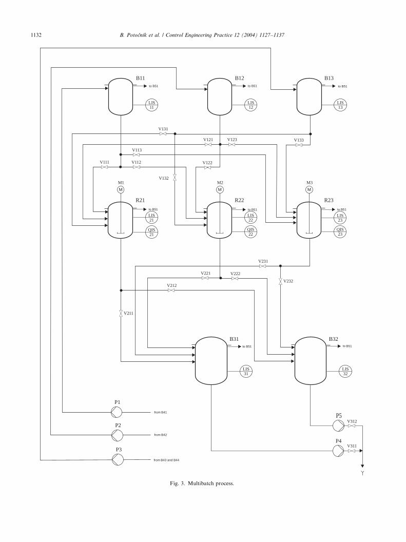
be seen in Fig. 3.
* The upper layer consists of the buffering tanks B11,B12 and B13, which are used for holding the rawmaterials ‘‘Yellow’’, ‘‘Red’’ and ‘‘White’’, respec-tively. Each of the buffer tanks is used exclusively forone raw material and can hold two batches ofsubstance.
* The middle layer consists of three stirred tank reactorsR21, R22 and R23. Each reactor can be filled fromany raw material buffer tank. This means that eachreactor can produce either ‘‘Blue’’ or ‘‘Green’’. Theproduction is done by first filling the reactor with onebatch of ‘‘Yellow’’ or ‘‘Red’’ and then neutralising itwith one batch of ‘‘White’’. Each reactor can containone batch of product resulting from two batches ofraw material.
* The lower layer consists of two buffer tanks B31 andB32 in which the products are collected from themiddle layer. Each of them is used exclusively for‘‘Blue’’ or ‘‘Green’’ and can contain three batches ofproduct.
The processing times of the plant (data of the optimalcontrol problem), presented in Table 2, are based on thefollowing specifications:
* The sampling time is Ts ¼ 1 s:* One batch of raw material is 850 ml (one batch ofproduct is therefore 1700 ml).
Neutralisation takes place while the NaOH is drainedinto the reactor and does not need any additional time.To summarise, the system can be influenced through
20 inputs, pumps P1-P5 and valves V111-V113, V121-V123, V131-V133, V211-V212, V221-V222 (see Fig. 3).Given that no additional time is needed to finish theneutralisation, it is natural to empty reactors R21-R23as soon the reactor is full. Similarly, the same can be
ARTICLE IN PRESS
P3
LIS11
B11
M
LIS22
QIS22
R22
M2
LIS32
B32
LIS31
B31
M
LIS23
QIS23
R23
M3
M
LIS21
QIS21
R21
M1
LIS13
B13
LIS12
B12
V113
V111 V112
V131
V121 V123
V212
V122
V221 V222
V231
V133
V132
V211
V232
P2
P1
to B51to B51
to B51 to B51 to B51
to B51 to B51
P5
P4
V312
V311
to B51
from B41
from B42
from B43 and B44
Fig. 3. Multibatch process.
B. Potocnik et al. / Control Engineering Practice 12 (2004) 1127–11371132

ARTICLE IN PRESS
Table 2
Processing times
Processes Times (s)
Pumping 1 batch ‘‘Yellow’’ into B11 12
Pumping 1 batch ‘‘Red’’ into B12 12
Pumping 1 batch ‘‘White’’ into B13 12
Draining 1 batch ‘‘Yellow’’ into R21 15
Draining 1 batch ‘‘Red’’ into R21 11
Draining 1 batch ‘‘White’’ into R21 10
Draining 1 batch ‘‘Yellow’’ into R22 12
Draining 1 batch ‘‘Red’’ into R22 13
Draining 1 batch ‘‘White’’ into R22 9
Draining 1 batch ‘‘Yellow’’ into R23 12
Draining 1 batch ‘‘Red’’ into R23 14
Draining 1 batch ‘‘White’’ into R23 13
Draining 1 batch ‘‘Blue’’ from R21 into B31 12
Draining 1 batch ‘‘Green’’ from R21 into B32 13
Draining 1 batch ‘‘Blue’’ from R22 into B31 12
Draining 1 batch ‘‘Green’’ from R22 into B32 12
Draining 1 batch ‘‘Blue’’ from R23 into B31 12
Draining 1 batch ‘‘Green’’ from R23 into B32 12
Pumping 3 batches ‘‘Red’’ out of B31 30
Pumping 3 batches ‘‘Green’’ out of B32 30
t0
1
ub V
111
Tmax B110
Fig. 4. The form of the input signal.
B. Potocnik et al. / Control Engineering Practice 12 (2004) 1127–1137 1133
also considered for buffer tanks B31 and B32. It isobvious that the number of inputs can be reduced to 12,i.e. three pumps (P1-P3) and nine valves (V111-V113,V121-V123, V131-V133) (see Fig. 3).
4.2. DHA and MLD model of a Multiproduct Batch
Plant
The Multiproduct Batch Plant was modelled as aDHA system. Due to the extensiveness of the resultingDHA model for the Multiproduct Batch Plant, we willprovide only the model for the reactor R21 (see Fig. 3).Reactor R21 can be filled from buffer tanks B11-B13
and emptied into buffer tanks B31 and B32. Themathematical model of the dynamics for reactor R21,considering all inputs and outputs, can be described as
dVR21
dt¼FVB11
ubV111þ FVB12
ubV121þ FVB13
ubV131
� FVB31ubV211
� FVB32ubV212
; ð8Þ
where VR21 represents the volume in reactor R21,FVB11
;FVB12and FVB13
represent the volume inflows frombuffer tanks in the first layer, while FVB31
and FVB32
represent the volume outflows to the buffer tanks in thethird layer. ubV111
; ubV121; ubV131
; ubV211; ubV212
are discreteinputs opening the corresponding valves. The inflowFVB11
can be modelled as a nonlinear relation
FVB11¼ KB11
ffiffiffiffiffiffiffiffiffiffiffiffiffiffi2ghB11
p; ð9Þ
where KB11 represents the appropriate constant para-meter. As we are actually interested only in the upper
bound of the finish times needed to fill or empty thereactor, the Eq. (9) can be simplified into
FVB11¼ LB11; ð10Þ
where is constant LB11 ¼ VmaxB11=TmaxB11
and is definedby the volume of the batch and the maximum timeTmaxB11
needed to empty one batch of raw material intothe reactor R21 (see Table 2). Once the input ubV111
is setto 1; it is controlled to have a form (Fig. 4) by using thereset timer. Of course, all remaining volume inflows andoutflows are modelled accordingly. Given that the DHAsystem is given in a discrete time and that the sampletime Ts ¼ 1 s, we obtain the following differenceequation for reactor R21:
VR21ðk þ 1Þ ¼VR21ðkÞ þ LB11ubV111ðkÞ
þ LB12ubV121ðkÞ þ LB13ubV131
ðkÞ
� LB31ubV211ðkÞ � LB32ubV212
ðkÞ: ð11Þ
The DHA system for reactor R21 is as follows. As, atmost, one input can be active at a time, the SAS of theform (1) contains six different operating modes eachdescribing one possible input combination. For theactive input ubV111
¼ 1 is
VR21ðk þ 1Þ
TB11ðk þ 1Þ
TB12ðk þ 1Þ
TB13ðk þ 1Þ
TB31ðk þ 1Þ
TB32ðk þ 1Þ
26666666664
37777777775
¼
1 0 0 0 0 0
0 1 0 0 0 0
0 0 0 0 0 0
0 0 0 0 0 0
0 0 0 0 0 0
0 0 0 0 0 0
26666666664
37777777775
VR21ðkÞ
TB11ðkÞ
TB12ðkÞ
TB13ðkÞ
TB31ðkÞ
TB32ðkÞ
26666666664
37777777775
þ
LB11
1
0
0
0
0
26666666664
37777777775
if iðkÞ ¼ 1; ð12Þ
where TB11; TB12; TB13; TB31; TB32 represent thedynamics of the counters (timers). Of course, for ubV111
¼1 only counter TB11 is active. Inactive mode andreaching the instance TmaxB11
of the counter TB11 is

ARTICLE IN PRESS
Table 3
Delivery times in [min:s] for raw material
Yellow Red White
0:00 0:10 0:00 4:20
0:30 0:40 0:30 5:30
1:10 1:50 2:00 6:20
4:20 5:30 2:20 6:55
5:40 6:50 3:00 7:10
6:45 7:50 3:35 8:00
B. Potocnik et al. / Control Engineering Practice 12 (2004) 1127–11371134
detected through the function of the EG:
½d1B11¼ 12½TB11p0;
½d2B11¼ 12½TB11XTmaxB11
: ð13Þ
Note that for the remaining five models the SAS and EGcan be modelled accordingly. As there are no logicstates, there is no FSM. The mode of the SAS is selectedthrough the following MS:
iðkÞ ¼
1 if ð%d1B11&%d2B11
ÞjubV111¼ 1
2 if ð%d1B12&%d2B12
ÞjubV112¼ 1
3 if ð%d1B13&%d2B13
ÞjubV113¼ 1
4 if ð%d1B31&%d2B31
ÞjubV211¼ 1
5 if ð%d1B32&%d2B32
ÞjubV212¼ 1
6 if ð%d1B11jubV111
j%d1B12jubV112
j%d1B13jubV113
j%d1B31
jubV211j%d1B32
jubV212Þ ¼ 0:
8>>>>>>>>>>>><>>>>>>>>>>>>:
ð14Þ
The HYSDEL code for the presented DHA system ofreactor R21 is given in Appendix A.The modelling procedure presented for reactor R21
can be also applied to all the remaining reactors andtanks. The obtained model is valid as long as theprocessing times reported in Table 2 are representing theupper bounds, i.e. robust according to the processingtimes uncertainties. Due to the extensiveness of thecomplete DHA system for the Multiproduct BatchPlant, modelled using the HYSDEL modelling lan-guage, the description is not given here but can be foundon the web site http://msc.fe.uni-lj.si/potocnik.Providing the DHA model of a Multiproduct
Batch Plant described by the HYSDEL modellinglanguage description, the HYSDEL tool generated theequivalent MLD form (2). The dimensions of thecorresponding variables are: xðkÞAR28 � f0; 1g6;ubðkÞAf0; 1g12; dðkÞAf0; 1g85; and zðkÞAR40: MatricesA; B1; B2; B3; C; D1; D2 and D3 have suitable di-mensions. Matrices E1 to E5 define 511 inequalities. Itcan be easily noticed that the system has 12 discreteinputs ubðkÞ and no continuous ones.
4.3. Control of the Multiproduct Batch Plant
Problem formulation:For a given initial condition control the production of
‘‘Blue’’ and ‘‘Green’’ to minimise the production time.Given that the raw material batches ‘‘Yellow’’, ‘‘Red’’
and ‘‘White’’ are delivered at fixed, given times whichare known in advance (see Table 3), the degrees offreedom are:
* the times at which one batch of ‘‘Yellow’’, ‘‘Red’’ or‘‘White’’ is emptied into a reactor
* the selection of a reactor in which the raw materialwill be emptied.
We focus on the problem of producing six batches of‘‘Blue’’ and ‘‘Green’’ constrained by the deliverytimes of batches ‘‘Yellow’’, ‘‘Red’’ and ‘‘White’’ givenin Table 3.The solution of a control problem is a control
sequence Ukfin�10 ¼ fubð0Þ;y; ubðkfin � 1Þg: Given that
we cannot influence the system through the first threeinputs (pumps P1-P3) because they are predefined by thedelivery times given in Table 3, at each time step onlynine remaining inputs (valves V111-V113, V121-V123and V131-V133) must be determined. The minimalproduction time can be over-bounded from Tables 2 and3, although such a time may not be feasible. The lastbatch of white is delivered after 480 seconds; addition-ally, 12þ 9þ 12 ¼ 33 seconds must be added to finishthe production, so the minimum time cannot be lessthan Tmin ¼ 513 s and consequently Ukfin�1
0 Af0; 1g4617
given that Ts ¼ 1 s: Because all the inputs are discrete,24617 possible combinations of the solution vector Ukfin�1
0
exist and searching for the solution through all thecombinations is practically impossible.According to the initial conditions and the cost
function criterion introduced earlier (see Eqs. (3)–(5)),we propose the following cost function:
Jiðv; kÞ ¼ ð3 � Vmax � vÞF þ k; ð15Þ
where Vmax is the volume of all products, v representsthe current volume of material pumped/emptied intothe first, second and third layer (see Fig. 3), k is thecurrent step and F is a factor whose properties will beexplained later. The goal (final state xfin) is reachedwhen v ¼ 3 � Vmax: The cost function value in the feasiblesolution is
Ji ¼ k: ð16Þ
According to (6), the cost function (15) has to bemonotonically increasing, i.e.
Jðvðk þ 1Þ; k þ 1Þ � JðvðkÞ; kÞ
¼ ð3 � Vmax � vðk þ 1ÞÞF þ ðk þ 1Þ
� ð3 � Vmax � vðkÞÞF � k
¼ �ðvðk þ 1Þ � vðkÞÞF þ 1X0: ð17Þ

ARTICLE IN PRESS
Table 5
Production time [min:s] and corresponding reactor
Blue Reactor Green Reactor
0:33 R22 0:52 R21
2:42 R23 2:21 R22
4:00 R21 3:21 R22
4:53 R22 5:52 R21
6:41 R22 7:32 R21
7:18 R22 8:23 R21
0 50 100 150 200 250 300 350 400 450 5000
0.5
1
1.5
Vb1
1(k)
0 50 100 150 200 250 300 350 400 450 5000
0.5
1
1.5
Vb1
2(k)
0 50 100 150 200 250 300 350 400 450 5000
0.5
1
1.5
Vb1
3(k)
0 50 100 150 200 250 300 350 400 450 5000
1
2
Vr21
(k)
0 50 100 150 200 250 300 350 400 450 5000
1
2
Vr22
(k)
0 50 100 150 200 250 300 350 400 450 5000
1
2
Vr23
(k)
5
k)
B. Potocnik et al. / Control Engineering Practice 12 (2004) 1127–1137 1135
and hence the parameter F must satisfy the condition
Fp1
vðk þ 1Þ � vðkÞ: ð18Þ
Note that according to property (4b), it holds that thedenominator in Eq. (18) �vðk þ 1Þ þ vðkÞp0 or vðk þ1Þ � vðkÞX0 for all k: In the worst case, the value forDv9vðk þ 1Þ � vðkÞ is defined through the estimation ofthe maximum change of volume in the system neglectingthe delivery times. If all three raw materials aredelivered, two reactors are filled and the third is emptiedinto a buffer tank at the same time, i.e. 3 � 0:85=12 (seeTable 2) for filling all the three tanks in upper layer,0:85=9 and 0:85=11 represent the filling of two reactorsusing maximum flow (shortest delivery time) and 1:7=12the emptying of the reactor into buffer tank, then thefollowing estimation for Dv is obtained
Dv ¼ 30:85
12þ0:85
9þ0:85
11þ1:7
12¼ 0:526: ð19Þ
Hence it follows that
Fp1
Dv¼
1
0:526¼ 1:90: ð20Þ
Regarding the node selection criterion, it is reasonableto choose the node that leads to the best (current)optimal solution, i.e. the node with the smallestassociated cost function value Ji at step k (the influenceof step instance k is the same, but the influence of v isgreater).
4.4. Results
Because of the complexity of the optimal controlproblem for the Multiproduct Batch Plant analysed inthe previous section, the algorithm provides an optimalsolution for a bounded time interval and a sub-optimalsolution for the complete optimal control problem. Thecomputational times refer to a MATLAB implementa-tion running on a Pentium III 667 MHz machine.The properties of the applied algorithm are presented
on a time interval kA½0; 50 and kA½0; 40 for two valuesof parameter, F ¼ 1:80 and 1.90. For the time intervalkA½0; 50; an approach based on enumeration wouldexamine 29�5062:9� 10135 possible solutions. Theresults are summarised in Table 4.
Table 4
Results on bounded time interval
Time int. Param. F Tree size CPU time
kA½0; 40 1.90 32205 0:22:26
kA½0; 40 1.80 36852 0:25:48
kA½0; 50 1.90 497799 5:48:10
kA½0; 50 1.80 608826 7:11:23
The results illustrate that parameter F exerts a greatinfluence on the size of the tree and, indirectly, on thetime needed to solve the optimisation problem.As the complexity of the optimisation problem grows
exponentially with the time horizon, a sub-optimalalgorithm based of additional knowledge on the processis preferred and gives satisfactory results in anacceptable time.We added a constraint on the tree size of 100,000
nodes (E1 hour) to the proposed algorithm and set theparameter F to 1.90. The solution is presented in Table 5
0 50 100 150 200 250 300 350 400 450 5000
Vb3
1(
0 50 100 150 200 250 300 350 400 450 5000
5
k
Vb3
2(k)
Fig. 5. Volumes in the tanks.

ARTICLE IN PRESSB. Potocnik et al. / Control Engineering Practice 12 (2004) 1127–11371136
and in Fig. 5. The first, and in this case the final, sub-optimal solution was obtained in just 27 seconds. Theproduction of six batches of ‘‘Blue’’ and ‘‘Green’’ can beachieved in 515 s: The lower bound to the globaloptimal solution ð513 sÞ is missed only by two seconds.We remark that the sub-optimal solution is feasible andcould also be optimal, but the algorithm would needmuch more time to prove optimality.
5. Conclusions
An optimal control problem for systems with discreteinputs only has been addressed. The problem was solved
HYSDEL CODE - Reactor R21
SYSTEM reactorR21 {
INTERFACE{
STATE {
REAL Tb11 [0,15
REAL Vr21 [0,1.
REAL Tb31 [0,12
INPUT {
BOOL uv111, uv1
PARAMETER {
REAL VB11=0.85,
REAL TB11=15, T
REAL VR21=1.7;
REAL TB31=12, T
IMPLEMENTATION {
AUX {
REAL Tb11p, Vb1
BOOL d1b11, d2b
REAL Tb12p, Vb1
BOOL d1b12, d2b
REAL Tb13p, Vb1
BOOL d1b13, d2b
REAL Tb31p, Vb3
BOOL d1b31, d2b
REAL Tb32p, Vb3
BOOL d1b32, d2b
AD {
d1b11 = Tb11 o=
d2b11 = TB11 - T
d1b12 = Tb12 o=
d2b12 = TB12 - T
d1b13 = Tb13 o=
d2b13 = TB13 - T
d1b31 = Tb31 o=
d2b31 = TB31 - T
d1b32 = Tb32 o=
d2b32 = TB32 - T
by combining hybrid modelling and reachabilityanalysis with a branch-and-bound technique. Thealgorithm abstracts the behaviour of the hybrid systeminto a ‘‘tree of evolution’’. The main advantage of theapproach is that the ‘‘tree’’ is cut from both sides, topand bottom, which result in considerable size reductionof the tree. The proposed approach was applied to aMultiproduct Batch Plant with satisfactory results.Future research will be devoted to adapting theproposed optimal control approach to model predictivecontrol techniques.
Appendix A
], Tb12 [0,11], Tb13 [0,10]; /� Timers �/7]; /� Volume in R21 �/], Tb32 [0,13];} /� Timers �/
12, uv113, uv211, uv212; }/� Inputs �/
VB12=0.85, VB13=0.85; /� Batch volume �/B12=11, TB13=10; /� Process times �//� Batch volume �/B32=13;} } /� Process times �/
1p; /� Aux. variables for states �/11; /� Aux. variable for timer status �/2p;
12;
3p;
13;
1p;
31;
2p;
32;}
0; /� Set timer status �/b11 o= 0;
0;
b12 o= 0;
0;
b13 o= 0;
0;
b31 o= 0;
0;
b32 o= 0;}

ARTICLE IN PRESS
DA {
Tb11p = {IF uv111 THEN Tb11+1}; /� Set timer value �/Vb11p = {IF uv111 THEN VB11/TB11}; /� Set volume �/Tb12p = {IF uv112 THEN Tb12+1};
Vb12p = {IF uv112 THEN VB12/TB12};
Tb13p = {IF uv113 THEN Tb13+1};
Vb13p = {IF uv113 THEN VB13/TB13};
Tb31p = {IF uv211 THEN Tb31+1};
Vb31p = {IF uv211 THEN VR21/TB31};
Tb32p = {IF uv212 THEN Tb32+1};
Vb32p = {IF uv212 THEN VR21/TB32};}
CONTINUOUS {
Vr21 = Vr21+Vb11p+Vb12p+Vb13p-Vb31p-Vb32p; /� Update states �/Tb11 = Tb11p;
Tb12 = Tb12p;
Tb13 = Tb13p;
Tb31 = Tb31p;
Tb32 = Tb32p;
MUST {
(B d1b11& B d2b11)->uv111; /� Control the input to have �/(B d1b12&B d2b12)->uv112; /� a specified form �/(B d1b13&B d2b13)->uv113;
(B d1b31&B d2b31)->uv211;
(B d1b32&B d2b32)->uv212;
/� Constrain inputs to one active input at a time �/(REAL uv111)+(REAL uv112)+(REAL uv113)+(REAL uv211)+(REAL
uv212)o=1;}}
}
B. Potocnik et al. / Control Engineering Practice 12 (2004) 1127–1137 1137
References
Antsaklis, P. J. (Ed.). (2000). Special issue on hybrid systems: Theory
and applications. Proceedings of the IEEE, 88 (7).
Barton, P. I., Banga, J. R., & Gal!an, S. (2000). Optimization of hybrid
discrete/continuous dynamic systems. Computers and Chemical
Engineering, 24, 2171–2182.
Bauer, N. (2000). A demonstration plant for the control and
scheduling of multi-product batch operations. Techinical Re-
port—VHS Case Study 7, University of Dortmund, Dortmund.
Bauer, N., Kowalewski, S., Sand, G., & L .ohl, T. (2000). A case study:
Multi product batch plant for the demonstration of control and
scheduling problems. ADPM2000 conference proceedings, Dort-
mund, Germany (pp. 383–388).
Bemporad, A., Giovanardi, L., & Torrisi, F. D. (2000). Performance
driven reachability analysis for optimal scheduling and control of
hybrid systems. In Proceedings of the 39th IEEE conference on
decision and control, Sydney, Australia (pp. 969–974).
Bemporad, A., & Mignone, D. (2000). MIQP.M: A Matlab function
for solving mixed integer quadratic programs, ETH Zurich, code
available at http://control.ethz.ch/~hybrid/miqp.
Bemporad, A., & Morari, M. (1999). Control of systems integrating
logic, dynamic, and constraints. Automatica, 35(3), 407–427.
Bemporad, A., Torrisi, F. D., & Morari, M. (2001). Discrete-time
hybrid modeling and verification of the batch evaporator process
benchmark. European Journal of Control, 7(4), 382–399.
Cassandras, C. G., Pepyne, D. L., & Wardi, Y. (2001). Optimal
Control of a Class of Hybrid Systems. IEEE Transanctions on
Automatic Control, 46(3), 398–415.
Gokbayrak, K., & Cassandras, C. G. (1999). A hierarchical decom-
position method for optimal control of hybrid systems. In
Proceedings of the 38th IEEE conference on decision and control,
Phoenix, AZ, USA (pp. 1816–1821).
Hedlund, S., & Rantzer, A. (1999). Optimal control of hybrid systems.
In Proceedings of the 38th IEEE conference on decision and control,
Phoenix, AZ, USA (pp. 3972–3976).
Heemels, W. P. M. H., De Schutter, B., & Bemporad, A. (2001).
Equivalence of hybrid dynamical models. Automatica, 37(7),
1085–1091.
Lincoln, B., & Rantzer, A. (2001). Optimizing linear system switching.
In Proceedings of the 40th IEEE conference on decision and control,
Orlando, FL, USA (pp. 2063–2068).
Rantzer, A., & Johansson, M. (2000). Piecewise linear quadratic
optimal control. IEEE Transanctions on Automatic Control, 45(4),
629–637.
Torrisi, F. D., & Bemporad, A. (2002). HYSDEL—A tool for
generating computational hybrid models, IEEE Transactions on
Control Systems Technology, in press.
Torrisi, F. D., Bemporad, A., Bertini, G., Hertach, P., Jost, D., &
Mignone, D. (2002). HYSDEL—User Manual, Techinical Report
AUT02-10, Automatic Control Laboratory, ETH, Zrich.