hybrid methodologies for symmetric and … also want to thank to my colleagues dr. daniel guimarans,...
TRANSCRIPT

Doctoral Thesis
Hybrid Methodologies forSymmetric and AsymmetricVehicle Routing Problems
AuthorRosa Herrero Anton
AdvisorDr. Juan Jose Ramos Gonzalez
PhD Program inInformatica Industrial: Tecniques Avancades de Produccio
Departament de Telecomunicacio i d’Enginyeria de SistemesUniversitat Autonoma de Barcelona
Bellaterra, November 2015


Dr. Juan Jose Ramos Gonzalez, Associate Professor at the Universitat Autono-ma de Barcelona,
CERTIFIES:
That the thesis entitled Hybrid Methodologies for Symmetric and Asymmet-ric Vehicle Routing Problems and submitted by Rosa Herrero Anton in partialfulfillment of the requirements for the degree of Doctor, has been developed and writtenunder his supervision.
Dr. Juan Jose Ramos Gonzalez Rosa Herrero AntonThesis Director PhD Student
PhD Program inInformatica Industrial: Tecniques Avancades de ProduccioDepartament de Telecomunicacio i d’Enginyeria de SistemesUniversitat Autonoma de Barcelona
Sabadell, November 2015


“Time is life itself, and life resides in the human heart.”Michael Ende, Momo
“Someone is sitting in the shade today becausesomeone planted a tree a long time ago.”
Warren Buffett


Acknowledgement
First, I am greatful to my advisor, Dr. Juanjo Ramos for his support along this thesiswork, and also for giving me the opportunity to participate in very interesting experienceduring these last years.
There are two professors that I would especially like to express my gratitude. Thefirst one is for me my second advisor Dr. Angel A. Juan, who guided and encouragedme during my PhD, even also giving me the chance to stay at Universitat Oberta deCatalunya. The second one is Dr. Marco Gavanelli, who led and supported me during mystay at Universita degli Studi di Ferrara, I marveled at his technical research. Probably,this PhD thesis would have not been possible without their help.
I also want to thank to my colleagues Dr. Daniel Guimarans, Dr. MassimilianoCattafi, Dr. Jose Caceres for their willingness to help me, for their support in ourarticles and for the time enjoyed together.
Thanks to my mates who have shared with me all these years, some years at UABand others despite the distance: Catya Zuniga, Jose David Rojas, Adriana Ramırez,Hector Delgado, Helena Martın, Lars Peters, Luis Blanco, Monica Gutierrez, DavidBote... Thank you guys for the coffee time and so many interesting discussions, mostlywithout any relevance to this thesis, but otherwise essential for happiness!
I cannot forget to express my gratitude again to Catya Zuniga, who I am lucky tocount among my closest friends. Thank you for your friendship and love, without youfinishing this thesis would have been almost impossible.
Por ultimo, pero el mas importante de todos, quiero agradecer a mi marido Javi supaciencia y amor, y tambien a toda mi familia, especialmente a mis padres Cruz y Remi,y a mi tıo Jose Marıa.
G�r�a�c�i�as �a� �t�o�d�o�s!
vii


Brief Contents
Introduction
Methodologies
Part I: Symmetric Problems
Chapter 1: Traveling Salesman Problem
Chapter 2: Capacitated Vehicle Routing Problem
Chapter 3: Workload-Balanced and Loyalty-Enhanced Home Health Care
Part II: Asymmetric Problems
Chapter 4: Asymmetric Traveling Salesman Problem
Chapter 5: Asymmetric Capacitated Vehicle Routing Problem
Chapter 6: Asymmetric and Heterogeneous Capacitated Vehicle Routing Problem
Contributions, Conclusions, Future Research and Publications
References
ix


Contents
Page
List of Tables and Figures xvii
List of Algorithms xix
Introduction 1
Introduction . . . . . . . . . . . . . . . . . . . . . . . . . . . . . . . . . . . . . . 1
Objectives . . . . . . . . . . . . . . . . . . . . . . . . . . . . . . . . . . . . . . . 5
Synopsis . . . . . . . . . . . . . . . . . . . . . . . . . . . . . . . . . . . . . . . . 6
Methodologies 7
Lagrangian Relaxation . . . . . . . . . . . . . . . . . . . . . . . . . . . . . . . . 7
Metaheuristics . . . . . . . . . . . . . . . . . . . . . . . . . . . . . . . . . . . . 17
Part I: Symmetric Problems 21
1 Traveling Salesman Problem 23
1.1 Problem Definition . . . . . . . . . . . . . . . . . . . . . . . . . . . . . . 24
1.2 Its variants . . . . . . . . . . . . . . . . . . . . . . . . . . . . . . . . . . 26
1.3 Literature Review . . . . . . . . . . . . . . . . . . . . . . . . . . . . . . 28
1.4 Lagrangian Dual Problem . . . . . . . . . . . . . . . . . . . . . . . . . . 31
1.5 An Experiment in Convergence . . . . . . . . . . . . . . . . . . . . . . . 32
1.6 Tailored Lagrangian Metaheuristic . . . . . . . . . . . . . . . . . . . . . 33
1.7 Computational Results . . . . . . . . . . . . . . . . . . . . . . . . . . . 38
1.8 Conclusions . . . . . . . . . . . . . . . . . . . . . . . . . . . . . . . . . . 41
2 Capacitated Vehicle Routing Problem 43
2.1 Problem Definition . . . . . . . . . . . . . . . . . . . . . . . . . . . . . . 44
2.2 Literature Review . . . . . . . . . . . . . . . . . . . . . . . . . . . . . . 46
2.3 Technologies used . . . . . . . . . . . . . . . . . . . . . . . . . . . . . . 47
2.4 The methodology in detail . . . . . . . . . . . . . . . . . . . . . . . . . 49
2.5 Computational Results . . . . . . . . . . . . . . . . . . . . . . . . . . . 52
2.6 Conclusions . . . . . . . . . . . . . . . . . . . . . . . . . . . . . . . . . . 56
xi

xii CONTENTS
3 Workload-Balanced and Loyalty-Enhanced Home Health Care 59
3.1 Problem Definition . . . . . . . . . . . . . . . . . . . . . . . . . . . . . . 60
3.2 Literature Review . . . . . . . . . . . . . . . . . . . . . . . . . . . . . . 64
3.3 The Methodology in detail . . . . . . . . . . . . . . . . . . . . . . . . . 67
3.4 Experiments and Results . . . . . . . . . . . . . . . . . . . . . . . . . . 78
3.5 Conclusions . . . . . . . . . . . . . . . . . . . . . . . . . . . . . . . . . . 89
Part II: Asymmetric Problems 91
4 Asymmetric Traveling Salesman Problem 93
4.1 Problem Definition . . . . . . . . . . . . . . . . . . . . . . . . . . . . . . 95
4.2 Literature Review . . . . . . . . . . . . . . . . . . . . . . . . . . . . . . 96
4.3 Our proposed TLM for the asymmetric case . . . . . . . . . . . . . . . 99
4.4 Computational Results . . . . . . . . . . . . . . . . . . . . . . . . . . . 102
4.5 Conclusions . . . . . . . . . . . . . . . . . . . . . . . . . . . . . . . . . . 106
5 Asymmetric Capacitated Vehicle Routing Problem 109
5.1 Problem Definition . . . . . . . . . . . . . . . . . . . . . . . . . . . . . . 110
5.2 Literature Review . . . . . . . . . . . . . . . . . . . . . . . . . . . . . . 111
5.3 The SR-GCWS-CS algorithm adapted for the ACVRP . . . . . . . . . . 112
5.4 Computational Results . . . . . . . . . . . . . . . . . . . . . . . . . . . 114
5.5 Conclusions . . . . . . . . . . . . . . . . . . . . . . . . . . . . . . . . . . 117
6 Asymmetric and Heterogeneous Vehicle Routing Problem 119
6.1 Problem Definition . . . . . . . . . . . . . . . . . . . . . . . . . . . . . . 120
6.2 Literature Review . . . . . . . . . . . . . . . . . . . . . . . . . . . . . . 121
6.3 The SR-GCWS-CS algorithm adapted for the AHVRP . . . . . . . . . 124
6.4 Experimental Design . . . . . . . . . . . . . . . . . . . . . . . . . . . . . 125
6.5 Computational Results . . . . . . . . . . . . . . . . . . . . . . . . . . . 126
6.6 Conclusions . . . . . . . . . . . . . . . . . . . . . . . . . . . . . . . . . . 132
Contributions 133
Main contributions . . . . . . . . . . . . . . . . . . . . . . . . . . . . . . . . . . 133
Conclusions . . . . . . . . . . . . . . . . . . . . . . . . . . . . . . . . . . . . . . 135
Future Research . . . . . . . . . . . . . . . . . . . . . . . . . . . . . . . . . . . 135
Publications . . . . . . . . . . . . . . . . . . . . . . . . . . . . . . . . . . . . . . 137
References 139

CONTENTS xiii
Appendices 159
Appendix A Spanish Airports Problem 161


List of Tables and Figures
Page
Figure 1: General outline of this thesis. . . . . . . . . . . . . . . . . . . . . 4
Figure 2: Applications of Lagrangian Relaxation . . . . . . . . . . . . . . . 9
Figure 3: Epigraph of an optimization problem and of a relaxation . . . . . 14
Figure 4: Form of the Lagrangian dual function . . . . . . . . . . . . . . . . 15
Figure 1.1: Icosian Game . . . . . . . . . . . . . . . . . . . . . . . . . . . . . 26
Figure 1.2: Hamiltonian path . . . . . . . . . . . . . . . . . . . . . . . . . . . 26
Figure 1.3: Convergence of the Subgradient Algorithm with different stepsizes for Spanish Airports problem. . . . . . . . . . . . . . . . . . 33
Figure 1.4: Movements of the proposed heuristic . . . . . . . . . . . . . . . . 36
Table 1.5: Summary of results obtained applying the Tailored LagrangianMetaheuristic for the Traveling Salesman Problem. . . . . . . . . 38
Table 1.6: Results obtained applying the Tailored Lagrangian Metaheuristicfor the Traveling Salesman Problem . . . . . . . . . . . . . . . . . 39
Figure 1.7: Convergence of LB, L, and UB in some problems. . . . . . . . . 40
Table 2.1: Results for 50 classical benchmark instances. . . . . . . . . . . . . 54
Table 2.2: Comparison between the proposed algorithm and other approa-ches for some classical benchmark instances. . . . . . . . . . . . . 55
Table 3.1: Excerpt of the services with average service time . . . . . . . . . 61
Figure 3.2: Histogram of the frequency of service durations in a typical day . 62
Figure 3.3: The 9 zones in which the city is divided, with shown the locationof the patients . . . . . . . . . . . . . . . . . . . . . . . . . . . . . 63
Figure 3.4: Example situation 1: There is a patient that lives rather far fromthe hospital, and also requires a long service time. . . . . . . . . . 72
Figure 3.5: Example situation 2: There are 5 patients with different servicetime. . . . . . . . . . . . . . . . . . . . . . . . . . . . . . . . . . . 72
Figure 3.6: Maximum Week Workload of the nurses in the four real instances,computed by the various algorithms, and compared to the Hand-Made Solution. . . . . . . . . . . . . . . . . . . . . . . . . . . . . 79
Figure 3.7: Loyalty penalization obtained by the algorithms in the four realinstances, compared with the Hand-Made Solution. . . . . . . . . 79
xv

xvi LIST OF TABLES AND FIGURES
Figure 3.8: (Near)Pareto front of solutions of one weekly instance, reportingalso the hand-made solution. . . . . . . . . . . . . . . . . . . . . . 81
Figure 3.9: Absolute deviation from the mean of the nurses’ week workloadobtained with the two objective functions in the four real in-stances, compared with the Hand-Made Solution. . . . . . . . . . 83
Figure 3.10: Distribution of the week workload to the various nurses in thebest solutions found using the two objective functions. . . . . . . 83
Figure 3.11: Absolute deviation from the mean of the service time and theweek workload obtained by the various algorithms in real week 1. 84
Figure 3.12: Total Travel time of the nurses obtained with the two objectivefunctions in the four real instances, compared with the Hand-Made Solution. . . . . . . . . . . . . . . . . . . . . . . . . . . . . 84
Table 3.13: Classes of instances in the crafted set. . . . . . . . . . . . . . . . 86
Table 3.14: Number of solved instances in the crafted set. . . . . . . . . . . . 86
Figure 3.15: Average of the different components of the objective function inthe 12 classes of instances. . . . . . . . . . . . . . . . . . . . . . . 87
Figure 3.16: Absolute Deviation from the mean of the Week Workload andthe Service Time of the nurses. . . . . . . . . . . . . . . . . . . . 88
Figure 4.1: Comparative of a tour in Barcelona according the symmetry orasymmetry of the distance cost. . . . . . . . . . . . . . . . . . . . 94
Table 4.2: Results for 27 ATSP instances. . . . . . . . . . . . . . . . . . . . 103
Table 4.3: Comparison between both proposed algorithms, the original TLMfor the TSP and the adaptation for the ATSP, for 33 TSP instances.104
Table 4.4: (continued) Comparison between both proposed algorithms, theoriginal TLM for the TSP and the adaptation for the ATSP, for33 TSP instances. . . . . . . . . . . . . . . . . . . . . . . . . . . . 105
Table 4.5: Summary of results obtained comparing both algorithms for 33TSP instances. . . . . . . . . . . . . . . . . . . . . . . . . . . . . 106
Figure 4.6: Comparison of CPUtime between both proposed algorithms, theoriginal TLM for the TSP and the adaptation for the ATSP, for33 TSP instances. . . . . . . . . . . . . . . . . . . . . . . . . . . . 106
Figure 5.1: Merging two routes with opposite orientation. . . . . . . . . . . . 113
Table 5.2: Comparison of results for AVRP instances. . . . . . . . . . . . . . 116
Table 6.1: Summary of published HVRP studies. . . . . . . . . . . . . . . . 122
Table 6.2: Summary of published Rich HVRP studies. . . . . . . . . . . . . 123
Table 6.3: Experimental results with different fleet configurations for small-size instances using random locations for nodes. . . . . . . . . . . 127
Table 6.4: Experimental results with different fleet configurations for small-size instances using grid locations for nodes. . . . . . . . . . . . . 128
Table 6.5: Experimental results with different fleet configurations for medium-size instances using random locations for nodes. . . . . . . . . . . 129

LIST OF TABLES AND FIGURES xvii
Table 6.6: Experimental results with different fleet configurations for medium-size instances using grid locations for nodes. . . . . . . . . . . . . 130
Figure 6.7: Surface Plot of Average Gap vs. Fleet Configuration . . . . . . . 131


List of Algorithms
PageAlgorithm 1: The Subgradient Algorithm . . . . . . . . . . . . . . . . . . . . 15Algorithm 2: Prim’s Algorithm for the 1-Tree . . . . . . . . . . . . . . . . . . 32Algorithm 3: Tailored LR-based method for the TSP . . . . . . . . . . . . . 35Algorithm 4: Heuristic to obtain feasible solution for a 1-Tree . . . . . . . . . 37Algorithm 5: Multi Start Approach . . . . . . . . . . . . . . . . . . . . . . . 50Algorithm 6: Variable Neighborhood Descent Algorithm . . . . . . . . . . . . 51Algorithm 7: Large Neighborhood Search for the Home Health Care . . . . . 77Algorithm 8: Edmonds’ Algorithm for the 1-Arborescence . . . . . . . . . . . 100Algorithm 9: Heuristic to feasible dual solution for asymmetric cases . . . . . 101Algorithm 10: SR-GCWS-CS algorithm for the Asymmetric case . . . . . . . 113Algorithm 11: The Asymmetric SR-GCWS-CS for Heterogeneous Fleets . . . 125
xix


Introduction
Over the last decades, globalization has driven the adaptation of the transport and logis-tics sector to new social demands. At the same time, transport has been the backboneof globalization. This social need creates ambitious consumers who need their productsquickly and an affordable price often unaware of their origin, transport mode or envi-ronmental aspects, among other factors. Nevertheless, to satisfy customer demands, itis needed to find the cheapest transport mode, which in turn means the improvementof transport logistics of the products. Therefore, these demands require an increas-ingly flexible service to meet customer requirements, and in addition companies want anefficient and productive transport.
In addition, it is important to know what kind of product demand is considered.Mainly, there are two types of demands: monotonous demand that requires a stabletransport throughout months; and a more volatile demand which will depend on someperishable factors, such as seasons, trending or brief consumer need. This second demandhas to be followed by a flexible transport network which has to be adaptable to newcircumstances. It must also be considered the dependence on the product characteristics,such as dimensions and weight, or if any special condition is needed for fragility orconservation.
Furthermore, according to the previously mentioned factors, it must be selected theproper transportation mode. Transport could be carried out by sea, air or land. Airand sea routes are commonly used for large quantities or long distances, their itinerariesare established and are not flexible. In contrast, land transport is really flexible and itallows to quickly adapts to the customer demand.
Therefore, road transport is a vital link in the increasingly complex sector of transportand logistics, which takes freight to ports and terminals and distribute urban goodsbetween warehouses and retail outlets, in order to arrive to the customers.
The sector of transport and logistics in the Spanish economy represents the 3% ofGross Domestic Product (GDP). The total cost of this sector was estimated about 25,000M¤ in 2011. Additionally, freight transport represents 60% of the total cost which wasabout 15,000 M¤ (OTLE, 2015).
The Spanish freight transport is characterized as predominantly national, with ashare of 71% compared to 29% international. Road traffic transports 94.6% of the totaltones nationwide in 2013 (OTLE, 2015).
Transportation costs cannot be neglected, improving the competitiveness of road
1

2 Introduction
transport is essential for companies in this sector, not only at Spanish scale but alsoat worldwide. In Europe, transportation often accounts for between one-third and two-thirds of total logistics costs –i.e., between 9% and 10% of the Gross National Product(GNP) for the Europe economy and also between 10% and 20% of a products price, sotransportations importance and key role is undeniable (Khooban, 2011).
The need for optimizing the road transportation affects to both public and privatesectors, given that it is an ambivalent issue: on the one hand, it brings great benefits forindividuals and economies; on the other hand, it may bring some negative side effectson quality of life and health, such as noise or air pollution, increasing greenhouse gases,waste products, even accidents death injuries.
Traveling Salesman Problems (TSP) and Vehicle Routing Problems (VRP) deal withthe physical distribution of goods from a central depot to customers. The TSP wasfirst formulated by Karl Menger (1930), the origin of the name “traveling salesmanproblem” is a bit of a mystery without any recognized creator. Nevertheless, the VRPfirst appeared defined by Dantzig and Ramser (1959). A wide number of related problemshave been developed during the last decades, each of them considering different setsof characteristics and constraints. Usually, the main goal of this set of problems isto minimize distance-based costs associated with the distribution of products amongcustomers while satisfying customers’ demands.
Both problems belong to the field of combinatorial optimization, and they are one ofthe most challenging problems because of they belong to the NP-Hard problems class,(Lenstra & Kan, 1981), meaning that they are not solvable in polynomial time, i.e.,there is no efficient algorithm to solve these problems that has been proved to solvecorrectly all scenarios, and whose worst-case running time is bounded by a polynomialtime function which depends on the scenarios’ size.
According to K. L. Hoffman et al. (2013), the TSP has commanded much attentionof mathematicians and computer scientists specifically because it is easy to describe andreally difficult to solve, in addition it has a lot of applications in the real life. Therefore,this problem has been a great engine of discovery for general purpose techniques inapplied mathematics (Applegate et al., 2006). Some areas to which TSP research hasmade fundamental contributions are: Mixed-Integer Programming, Branch-and-Boundmethod, and some metaheuristics such as Local-Search algorithms, Simulated Annealing,Neural Network, and Genetic Algorithms.
The TSP algorithm developed by Held and Karp (1970) carried the best-knownguarantee on the running time of a general solution method for the problem for over 40years. Recently, a TSP solver named Concorde developed by Applegate et al. (2015) isthe best-known exact method, it has been used to obtain the optimal solutions to 106 ofthe 110 TSPLIB instances; the largest having 85,900 cities. Currently, the heuristic ofLin and Kernighan (1973) effectively modified by Helsgaun (2000) holds the record forthe best instances of problems with unknown optimal (DIMACS TSP Challenge 2002 )with sizes ranging from 1,000 to 10,000,000 nodes.
The VRP is also one of the most researched problems, due to this field has been ex-ploited dramatically partly driven by the industrial applicability. In the early years, spe-

Introduction 3
cialized heuristics were typically developed for solving the VRP. Then, more generic solu-tion schemes as metaheuristics were designed, among them it can be found research aboutAnt Colony Optimization, Genetic Algorithms, Greedy Randomized Adaptive SearchProcedure, Simulated Annealing, Tabu Search, and Variable Neighborhood Search. Theinterest about hybrid optimization methods has grown very fast for the last decade.
From the industrial point of view, these problems characterize a family of differ-ent distribution problems which, one way or another, are presented in real problems.However, most of the real applications are not represented by the classical variants, forinstance, most VRP related academic articles assume the existence of a homogeneousfleet of vehicles and/or a symmetric cost matrix. These assumptions are not alwaysreasonable in real-life scenarios. In real problems, it is needed to consider real-life con-straints, obtaining problems which are commonly known as Rich VRP.
Theoretical researches typically assume the symmetry of the distance-based costsassociated with traveling from one place to another. In fact, classical benchmark in-stances are based on Euclidean distances between each pair of locations, which result insymmetric costs. However, this metric is just a lower bound of the real distance betweentwo nodes connected by a transport network or highway. The real distance will dependupon the specific location of the nodes in the territory and also on the structure of theroad network that connects them, which commonly are oriented networks, Rodrıguezand Ruiz (2012b) suggest that real distances might not have to be symmetric. Fur-thermore, Rodrıguez and Ruiz (2012a) demonstrate and measure, symmetric solutions(those obtained with symmetric and Euclidean distance matrices) have little in com-mon with regard to sequence and total distance with real solutions (those obtained withasymmetric and real distances).
Another frequent assumption is the existence of a homogeneous fleet of vehicles withlimited capacity. However, most road-transportation companies own a heterogeneousfleet of vehicles. This diversity in the vehicles’ capacity might be due to the fact thatdifferent customers and locations might require different types of vehicles, e.g., narrowroads in a city, available parking spaces, vehicle weight restrictions on certain roads, etc.Another reason for owning vehicles with distinct capacities is the natural diversity thatarises when vehicle acquisitions are made over time.
In this scenario, it becomes evident the need of developing new methods, models andsystems to give support to the decision-making process so that optimal strategies canbe chosen in road transportation.
The main goal of this thesis is to introduce hybrid methodologies that integrateseveral techniques to efficiently solve rich Vehicle Routing Problems with realistic con-straints. This thesis is outlined in Figure 1, it starts with theoretical problems andevolves into more realistic scenarios tackling six combinatorial problems related to roadtransport. It is explored the potential of the Lagrangian Relaxation (LR) for solvingrich and realistic problems. Due to the evolution of the scenarios chosen –from Travel-ing Salesman Problem to Asymmetric and Heterogeneous Vehicle Routing Problem– LRis combined into a hybrid method adding new techniques when required.
This thesis starts addressing the TSP, which is a well-known theoretical problem.

4 Introduction
TSP ATSP
CVRP ACVRP AHVRPHHC
TLM
Adapted
SR-GCWS
Adapted
SR-GCWS
Adapted TLM
Hybrid method
using TLM
Hybrid method
using TLM
Asymmetric costs
Heterogeneous fleetAsymmetric costs
Applications
Figure 1: General outline of this thesis.
The problem deals with finding the shortest path of a salesman who is required to visitonce and only once each different customers starting from a depot, and returning tothe same depot. LR is used to exploit the structure of the problem reducing consid-erably its complexity by moving hard-to-satisfy constraints into the objective function,associating a penalty in case they are not satisfied. For that purpose, a metaheuristic–named Tailored Lagrangian Metaheuristic (TLM)– based on the Lagrangian Relaxationis developed.
The Asymmetric version of the TSP (ATSP) has been chosen in order to illustrate theeffects of the frequent assumption of the symmetry of the distance-based costs associatedwith traveling from one place to another. Therefore, the proposed TLM is adapted forthe asymmetric scenarios.
The Capacitated Vehicle Routing Problem (CVRP) consists of determining the op-timal set of routes for a fleet of vehicles to deliver goods to a given set of customers,it is a generalization of the TSP. In the model proposed in this thesis, the CVRP hasbeen divided into two subproblems, concerning customers’ allocation and routing opti-mization separately. The first one aims to assign customers to vehicles fulfilling capacitylimitations. Then, it is used to solve each independent route giving the best solution fora particular allocation. Thus, routing optimization process can be viewed as solving aset of independent symmetric TSP. A hybrid approach proposes a Multi-Start VariableNeighborhood Descent structure whose local search process is supported by ConstraintProgramming (CP) for solving the customers’ allocation and our TLM metaheuristic forsolving independently each TSP.
It is presented a practical application concerning the Home Health Care (HHC)service in the municipality of Ferrara, Italy. This real problem consists on assigning pa-tients’ services to nurses which travel to each patient’s home. Therefore, it is defined thenurse itineraries which considers the following optimization aspects: the nurse workloadsare balanced, patients are preferentially served by a single nurse or just a few ones, and

Introduction 5
the overall travel time is minimized. A hybrid methodology based on CP and our TLMis considered for addressing this real problem.
Given the fact that urban networks are asymmetric and to contribute to closing thegap between theory and practice, the Asymmetric version of the CVRP (ACVRP) hasbeen considered. A hybrid methodology based on the randomized Clarke and WrightSavings algorithm (SR-GCWS), developed by Juan et al. (2010), is adapted for theasymmetric scenarios. The Clarke and Wright Savings heuristic (CWS), presented byClarke and Wright (1964), is one of the most commonly cited methods in the VRPliterature. Our proposed algorithm combines a randomized savings heuristic with twolocal search processes specifically designed for the asymmetric nature of costs in real-lifescenarios.
The ACVRP with heterogeneous fleet of vehicles (AHVRP) has been chosen in orderto illustrate the effects of the frequent assumption of the existence of a homogeneous fleetof vehicles. Our proposed Asymmetric SR-GCWS is combined with the modified Clarkeand Wright Savings heuristic presented by Prins (2002) for the HVRP. It is analyzed howrouting costs vary when slight deviations from the homogeneous fleet are considered, i.e.,how marginal costs/savings change when a few ’standard‘ vehicles in the homogeneousscenario are substituted by other vehicles with different loading capacity.
Objectives
The objectives of this thesis can been summarized as follows:
• The development of a metaheuristic aimed to tackle the Traveling Salesman Prob-lem based on the Lagrangian Relaxation.
• This metaheuristic should be efficient regarding the solution values and the compu-tational time. In addition, it should be flexible to be adaptable to the asymmetricscenarios.
• The integration of the developed metaheuristic into hybrid methodologies to tacklemore complex problems, like the Capacitated Vehicle Routing Problem.
• The application of the developed metaheuristic in a realistic scenario within ahybrid methodology, like the application in the Home Health Care in Ferrara,Italy.
• The study of different variants focusing on the impact that causes the asymmetryof the costs and the heterogeneity of the fleet.
• The development of a hybrid methodology adapted to deal with the asymmetricnature of costs, more concretely, to solve the Asymmetric Capacitated VehicleRouting Problem.
• The adaptation of the developed methodology considering heterogeneous fleets forsolving the Asymmetric and Heterogeneous Vehicle Routing Problem.
6 Introduction
Synopsis
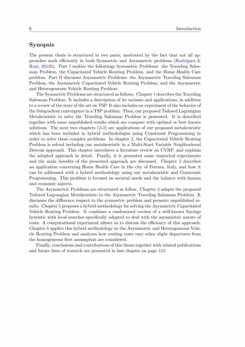
The present thesis is structured in two parts, motivated by the fact that not all ap-proaches work efficiently in both Symmetric and Asymmetric problems (Rodrıguez &Ruiz, 2012b). Part I tackles the followings Symmetric Problems: the Traveling Sales-man Problem, the Capacitated Vehicle Routing Problem, and the Home Health Careproblem. Part II discusses Asymmetric Problems: the Asymmetric Traveling SalesmanProblem, the Asymmetric Capacitated Vehicle Routing Problem, and the Asymmetricand Heterogeneous Vehicle Routing Problem.
The Symmetric Problems are structured as follows. Chapter 1 describes the TravelingSalesman Problem. It includes a description of its variants and applications, in additionto a review of the state of the art on TSP. It also includes an experiment of the behavior ofthe Subgradient convergence in a TSP problem. Then, our proposed Tailored LagrangianMetaheuristic to solve the Traveling Salesman Problem is presented. It is describedtogether with some unpublished results which are compare with optimal or best knownsolutions. The next two chapters (2-3) are applications of our proposed metaheuristicwhich has been included in hybrid methodologies using Constraint Programming inorder to solve these complex problems. In chapter 2, the Capacitated Vehicle RoutingProblem is solved including our metaheuristic in a Multi-Start Variable NeighborhoodDescent approach. This chapter introduces a literature review on CVRP, and explainsthe adopted approach in detail. Finally, it is presented some numerical experimentsand the main benefits of the presented approach are discussed. Chapter 3 describesan application concerning Home Health Care in the city of Ferrara, Italy, and how itcan be addressed with a hybrid methodology using our metaheuristic and ConstraintProgramming. This problem is focused on societal needs and the balance with humanand economic aspects.
The Asymmetric Problems are structured as follow. Chapter 4 adapts the proposedTailored Lagrangian Metaheuristic to the Asymmetric Traveling Salesman Problem. Itdiscusses the difference respect to the symmetric problem and presents unpublished re-sults. Chapter 5 proposes a hybrid methodology for solving the Asymmetric CapacitatedVehicle Routing Problem. It combines a randomized version of a well-known Savingsheuristic with local searches specifically adapted to deal with the asymmetric nature ofcosts. A computational experiment allows us to discuss the efficiency of this approach.Chapter 6 applies this hybrid methodology to the Asymmetric and Heterogeneous Vehi-cle Routing Problem and analyzes how routing costs vary when slight departures fromthe homogeneous fleet assumption are considered.
Finally, conclusions and contributions of this thesis together with related publicationsand future lines of research are presented in last chapter on page 133.
Methodologies
Lagrangian Relaxation
Lagrangian Relaxation (LR) is a well-known method to solve large-scale combinatorialoptimization problems, which is commonly used to generate lower bounds. It was namedfor the French mathematician Joseph Louis Lagrange, presumably due to the occurrenceof what we now call Lagrange multipliers in his calculus of variations, (Boyer, 1985). LRworks by moving hard-to-satisfy constraints into the objective function, associating apenalty in case they are not satisfied.
LR is strongly related to the earlier decomposition method of Dantzig and Wolfe(1960). However, the origin of the Lagrangian approach, as it exists today, was developedby Held and Karp (1970, 1971). An excellent introduction to LR can be found in(Fisher, 2004) along with a discussion of some early examples of Lagrangian heuristics.For a theoretical review of LR and a review of some methods for the dual problemlike the Subgradient algorithm, dual ascent methods, cutting plane method and columngeneration, see (Guignard, 2003).
LR is useful for exploiting the structure of the problem to reduce considerably theproblem complexity. Thus, the Lagrangian Problem needs less computational effort tofind solutions. However, one of its main drawbacks consist on finding optimal dualvariables normally called Lagrangian multipliers. Furthermore, for a given problem,there may exist different Lagrangian relaxations depending on the relaxed constraint.
When the Lagrangian Problem can be formulated as an Integer Linear Problem ora Mixed Integer Problem, then it can be solved in a optimal way by embedding LRinto the Branch-and-Bound (Geoffrion, 1974) or the Branch-and-cut (Edmonds, 1967)approaches. These methods provide both upper and lower bounds to the problem, andensure that the optimal solution is found. However, if the problem is NP-hard, largeproblems are not expected to be solved in a reasonable time.
In other cases, especially when the dual function is non-differentiable, some tech-niques can be useful to maximize the dual function of the Lagrangian relaxation, suchas the subgradient, bundle and surrogate. This techniques are simple and easy to im-plement and avoid using linear programming approaches. The Lagrangian multipliersstart with initial values and direct them toward the optimal value, this direction is calledsubgradient. However, these techniques are often terminated before an optimal value isattained, offering only a lower bound of the best objective value.
7

8 Methodologies
Within these techniques, the most widely used is the Subgradient Optimization al-gorithm (Shor, 1985). If the relaxed problem can be minimized obtaining a subgradient,then it guarantees convergence where the Lagrangian multipliers are updated along thesubgradient direction. One of the main drawbacks, remarked by Bertsekas (1999), is theneed of solving optimally all the subproblems, which may be slow to be of real practicalinterest.
On the other side, the Surrogate Gradient technique needs only an approximatesolution of the subproblem, so it may be desirable to obtain a proper direction with lesseffort. Nevertheless, it does not guarantee that the best bound obtained is equal to theoptimal value (Zhao et al., 1999).
Finally, the Bundle technique can provide better directions than the SubgradientAlgorithm. However, according to Hiriart-Urruty and Lemarechal (1993), to obtaineach direction require solving the subproblem many times. Subgradients from pastiterations are accumulated in a bundle, and a trial direction is obtained by quadraticprogramming based on the bundle information, for more information see (Kiwiel, 1996).This technique has not been of our interest given that it can increase the computationaleffort.
Literature review and Applications
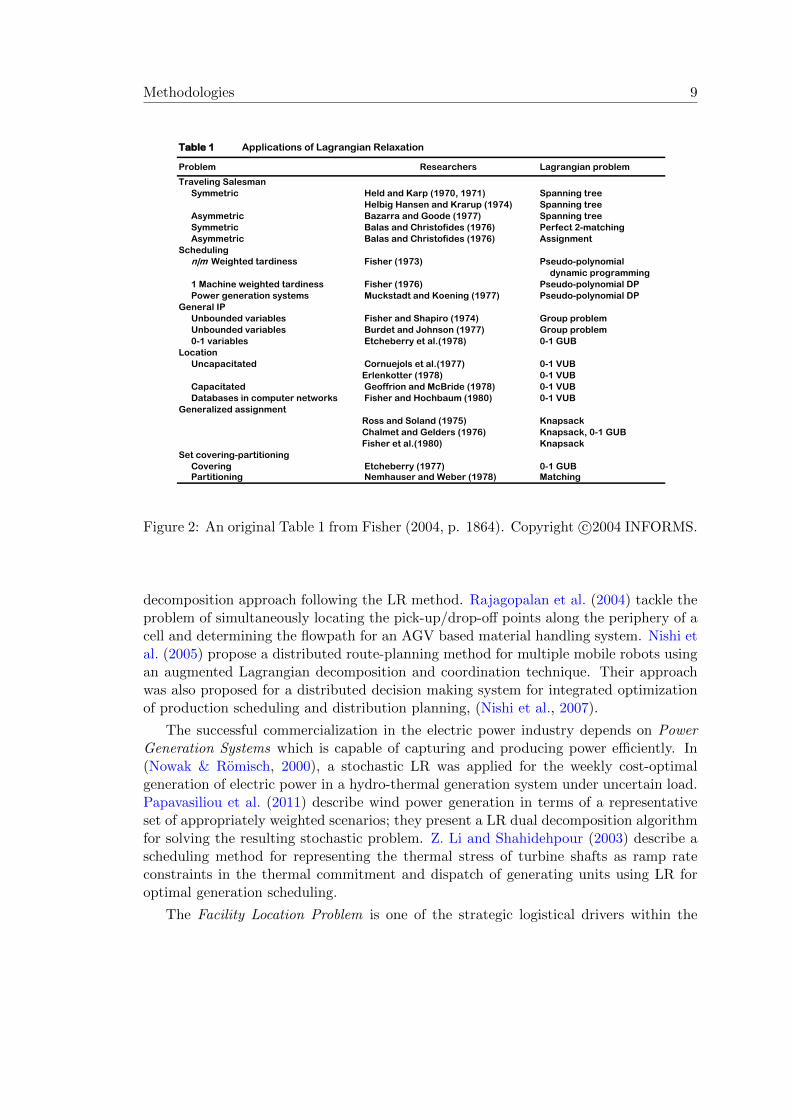
Lagrangian Relaxation has been widely used in diverse applications, figure 2 reprinteda table from Fisher (2004, p. 1864). This table shows the first applications of LR inthe 70’s. It can be noticed how for one problem there may exist different Lagrangianrelaxations depending on the relaxed constraint. Within this section a breve explanationof the most prominent applications will be given, we focus on the use of LR in both exactmethodologies and heuristic approaches.
Regarding to Manufacturing Scheduling Problems, Luh and Hoitomt (1993) achievegood decomposition of three scheduling problems relaxing one or more sets of constraints:the first problem considers scheduling single-operation jobs in identical machines; thesecond problem deals with scheduling multiple-operation jobs with simple fork / joinprecedence constraints on identical machines; lastly, the Job Shop Problem is consid-ered, where multiple-operation jobs with general precedence constraints are scheduledon multiple machine types. Nishi et al. (2010) address a LR-based method with cutgeneration for solving the hybrid flowshop scheduling problem to minimize the totalweighted tardiness. Mao et al. (2014) study a real-world hybrid flowshop problem aris-ing from the steel-making continuous casting process, which is the bottleneck of theiron and steel production process. Their paper is based on a time-index formulationand machine capacity relaxation, three LR subproblems are presented for addressingthis scheduling problem: job-level problems, batch-level problems, and machine-levelproblems.
To enable efficient transportation in manufacturing systems, it is necessary to gen-erate route planning of multiple Automated Guided Vehicles (AGVs) efficiently withoutcollision among them. A mixed integer programming model for AGVs planning and con-trol to minimize the total material handling cost is developed in (M. Chen, 1996) using a
Methodologies 9
Table 1 Applications of Lagrangian Relaxation
Problem Researchers Lagrangian problem
Traveling SalesmanSymmetric Held and Karp (1970, 1971) Spanning tree
Helbig Hansen and Krarup (1974) Spanning treeAsymmetric Bazarra and Goode (1977) Spanning treeSymmetric Balas and Christofides (1976) Perfect 2-matchingAsymmetric Balas and Christofides (1976) Assignment
Schedulingn|m Weighted tardiness Fisher (1973) Pseudo-polynomial
dynamic programming1 Machine weighted tardiness Fisher (1976) Pseudo-polynomial DPPower generation systems Muckstadt and Koening (1977) Pseudo-polynomial DP
General IP Unbounded variables Fisher and Shapiro (1974) Group problemUnbounded variables Burdet and Johnson (1977) Group problem0-1 variables Etcheberry et al.(1978) 0-1 GUB
Location Uncapacitated Cornuejols et al.(1977) 0-1 VUB
Erlenkotter (1978) 0-1 VUBCapacitated Geoffrion and McBride (1978) 0-1 VUBDatabases in computer networks Fisher and Hochbaum (1980) 0-1 VUB
Generalized assignmentRoss and Soland (1975) KnapsackChalmet and Gelders (1976) Knapsack, 0-1 GUBFisher et al.(1980) Knapsack
Set covering-partitioningCovering Etcheberry (1977) 0-1 GUBPartitioning Nemhauser and Weber (1978) Matching
Figure 2: An original Table 1 from Fisher (2004, p. 1864). Copyright c©2004 INFORMS.
decomposition approach following the LR method. Rajagopalan et al. (2004) tackle theproblem of simultaneously locating the pick-up/drop-off points along the periphery of acell and determining the flowpath for an AGV based material handling system. Nishi etal. (2005) propose a distributed route-planning method for multiple mobile robots usingan augmented Lagrangian decomposition and coordination technique. Their approachwas also proposed for a distributed decision making system for integrated optimizationof production scheduling and distribution planning, (Nishi et al., 2007).
The successful commercialization in the electric power industry depends on PowerGeneration Systems which is capable of capturing and producing power efficiently. In(Nowak & Romisch, 2000), a stochastic LR was applied for the weekly cost-optimalgeneration of electric power in a hydro-thermal generation system under uncertain load.Papavasiliou et al. (2011) describe wind power generation in terms of a representativeset of appropriately weighted scenarios; they present a LR dual decomposition algorithmfor solving the resulting stochastic problem. Z. Li and Shahidehpour (2003) describe ascheduling method for representing the thermal stress of turbine shafts as ramp rateconstraints in the thermal commitment and dispatch of generating units using LR foroptimal generation scheduling.
The Facility Location Problem is one of the strategic logistical drivers within the

10 Methodologies
supply chain which consist on locating a set of facilities and how to satisfy customers’demands from these open facilities so that the total cost which includes the facilityset up cost as well as the transportation cost is minimized. Nezhad et al. (2013) usea LR heuristic for the uncapacitated single-source multi-product facility location prob-lem. Gendron et al. (2013) present a Lagrangian-based Branch-and-Bound algorithm forthe two-level uncapacitated facility location problem with single-assignment constraints.Escobar et al. (2014) propose a granular variable Tabu Neighborhood Search for the ca-pacitated location-routing problem which uses LR method to group the customers intoclusters in the location phase. Jena et al. (2014) propose a LR heuristic for large-scaledynamic facility location with generalized modular capacities, that is, a multi-periodfacility location problem in which the costs of capacity changes are defined for all pairsof capacity levels.
The usage of the Internet has grown substantially in recent times, this has resulted inhigh volumes of data traffic. Replication of content and placing them on multiple serversis a method that is used to reduce latency. The Data Location Problem in informationnetworks deals with placing content so as to achieve better cost performance. Gavish andPirkul (1986) propose a branch-and-bound algorithm where the bounds are computedby LR followed by subgradient optimization for the data allocation problem and serverlocation problem. Nguyen et al. (2005) propose the Overlay Distribution Network asa cost-effective means to deliver the entertainment services which are expected to beincreasingly interactive, on demand and personalized. They solved this problem withan efficient LR heuristic where content clustering is employed to improve the heuristicrun time. Applegate et al. (2010) find a near-optimal solution with orders of magnitudespeedup relative to solving even the LP relaxation via standard software for the optimalcontent placement for a large-scale video-on-demand system.
Given certain jobs and certain agents, the Generalized Assignment Problem dealswith assigning each job to exactly one agent satisfying a resource constraint for eachagent in order to determine a minimum assignment cost. Posta et al. (2012) propose anexact algorithm for solving the generalized assignment problem by a simple depth-firstLagrangian branch-and-bound method, improved by variable-fixing rules to prune thesearch tree. Wu et al. (2014) propose a Lagrangian-based branch-and-cut algorithm forthe generalized assignment problem with min-max regret criterion under interval costs.Hanada and Hirayama (2011) use a distributed LR protocol for the over-constrainedgeneralized mutual assignment problem where, with no centralized control, multipleagents search for an optimal assignment of goods that satisfies their individual knapsackconstraints.
In a cross-dock, goods are unloaded from incoming trucks, consolidated accordingto their destinations, and then, loaded into outgoing trucks; all these with little or nostorage in between, the objective is minimizing the total material handling cost. Nassiefet al. (2015) present a new mixed integer programming formulation which is embeddedinto a Lagrangian relaxation that exploits the special structure of the problem to obtainbounds on the optimal solution value.
The Set Covering Problem (SCP) has been used as model in relevant applications, in

Methodologies 11
particular crew scheduling, where a given set of trips has to be covered by a minimum-cost set of pairings, i.e., a pairing is a sequence of trips that can be performed by asingle crew. The most successful heuristic algorithms for large scale SCP’s are based onLR, see (Caprara et al., 1996, 2000). Prins et al. (2006) deals with the bi-objective setcovering problem, the proposed approach is a two-phase heuristic method which has theparticularity to be a constructive method using the primal-dual Lagrangian relaxation.
With respect to the Traveling Salesman Problems and Vehicle Routing Problems(VRP), there has been some authors who use LR to find lower bounds, (Zamani & Lau,2010; Smith et al., 1990). Nevertheless, we are interested in those who have exploitedLR as exact methodologies or in heuristic approaches. It can be found a literature reviewon the use of LR for the TSP in chapter 1.
Balas and Christofides (1981) describe an algorithm for the Asymmetric TravelingSalesman Problem obtaining a Lagrangian relaxation based on the assignment problem.Their approach can be adapted to the symmetric TSP by using the 2-matching problemas a Lagrangian dual problem.
The Generalized Traveling Salesman Problem (GTSP) assumes that the nodes havebeen grouped into mutually exclusive and exhaustive node sets. It has to be found aminimum cost cycle which includes exactly one node from each node set. Fischetti et al.(1997a) apply Subgradient algorithm relaxing the fan inequalities plus the degree con-straints. Moreover, for each tour among clusters found during the Lagrangian relaxation,they obtain a new feasible solution through procedure RP2. For the asymmetric GTSP,Laporte et al. (1987) relax the subtour prevention constraints and a set of constraintswhich ensure that each set is visited. The relaxed problem is solved as an assignmentproblem in a branch-and-bound algorithm. Using the same relaxation, Noon and Bean(1991) employs a Lagrangian relaxation to compute a lower bound and a heuristicallydetermined upper bound are used to identify and remove arcs and nodes which areguaranteed not to be in an optimal solution.
Desrosiers et al. (1988) consider the problem of finding the minimum number of ve-hicles required to visit once a set of nodes subject to time window constraints, for ahomogeneous fleet of vehicles located at a common depot. Their present an optimalsolution approach using the augmented Lagrangian method. Two Lagrangian relax-ations are proposed: in the first one, the time constraints are relaxed producing networksubproblems which are easy to solve, but the bound obtained is weak; in the second re-laxation, constraints requiring that each node be visited are relaxed producing shortestpath subproblems with time window constraints and integrity conditions.
The Plate-Cutting Traveling Salesman Problem arises when parts are cut from largeplates of metal or glass, it requires the determination of a minimum-length tour such thatexactly one point must be visited on each given polygon. (Hoeft & Palekar, 1997) presenta Lagrangian decomposition of the problem and develop lower bounds and heuristicsbased on this decomposition which are embedded in a variable r-opt heuristic for theoverall problem.
The Train Timetabling Problem aims at determining a periodic timetable for a set oftrains that does not violate track capacities and satisfies some operational constraints.

12 Methodologies
Caprara et al. (2002) propose a graph theoretic formulation for the problem using adirected multigraph. A novel feature of their formulation is that the variables in theLagrangian relaxed constraints are associated only with nodes allowing a considerablespeed-up in the solution of the relaxed problem. The relaxation is embedded within aheuristic algorithm which makes extensive use of the dual information associated withthe Lagrangian multipliers.
For solving disruptions in the vehicle routing problem which are caused by vehiclesbreakdown or traffic accidents in the logistic distribution system, an urgency vehiclescheduling scheme is established based on the theory of disruption management. Ac-cording to the characteristics of the problem, X. Wang et al. (2010) apply a Lagrangianrelaxation approach to simplify and divide the Urgent Multi-Depot Vehicle Routing Prob-lem into two parts. The column generation and saving approach method are used re-spectively to obtain the solution, and then the subgradient optimization method is usedto iterate to get the Lagrangian multiplier. Moreover, in order to solve the infeasibilityproblem caused by the lack of convergence of the LR, an insertion algorithm is adoptedto obtain a feasible solution of the original problem.
The Vehicle Routing Problem with Time Windows is a generalization of the VRP.A solution to the this problem must ensure that the service of any customer startswithin a given time interval, a so-called time window. Fisher et al. (1997) present aLagrangian decomposition in which variable splitting is used to divide the problem intotwo subproblems: a semi-assignment problem and a series of shortest path problems withtime windows and capacity constraints. Kohl and Madsen (1997) propose a methodbased on a Lagrangian relaxation of the constraint set requiring that each customermust be served. They solved the Lagrangian dual problem using a combination of theSubgradient algorithm and the Bundle algorithm. Kallehauge et al. (2006) consider theLagrangian relaxation of the constraint set requiring that each customer must be servedby exactly one vehicle yielding a constrained shortest path subproblem. They presenta stabilized cutting-plane algorithm within the framework of linear programming forsolving the associated Lagrangian dual problem.
Lagrangian Dual Problem
Lagrangian relaxation is a method well suited for problems where the constraints canbe divided into two sets: constraints under which the problem is solvable very easily;and constraints that make it very hard to solve. The main idea is to relax the problemby removing these second constraints and putting them into the objective function.Consider the following Integer Linear Problem (ILP):
minx cx
s.t. Ax ≥ b (1)
Dx ≥ e (2)
x ∈ Zn+
Methodologies 13
where x is n × 1, b is m × 1, e is k × 1, and all other matrices have conformabledimensions. Let zP be the optimal value of the ILP problem.
It is assumed that the constraints of this problem 1 and 2 are independent. Moreover,supposing that the set of constraints 2 can be optimized very easily whereas the set ofconstraints 1 makes the problem intractable.
The Lagrangian Dual problem obtained from this ILP problem by taking into theobjective function the inequality Ax ≥ b (1) is:
L∗ = maxu∈Rm
L(u)
with Lagrangian function:
L(u) = minx cx+ u(Ax− b)s.t. Dx ≥ e
x ∈ Zn+
This Lagrangian Dual problem relaxes a set of constraints and introduce a Lagrangianmultiplier u for every constraint. Given that the relaxed set of constraints 1 is “greaterthan or equal to”, the Lagrangian multiplier vector u is of appropriate dimensions m andnon-negative components. Note also that the original ILP is a minimization problem,so its Lagrangian dual problem maximizes.
The original ILP problem can be relaxed into different problems depending on therelaxed constraints. If the chosen relaxation exploits the structure of the problem, theresulting dual problem can efficiently compute the optimal value for a fixed vector u andthen it is easier to solve than the original problem.
Nemhauser and Wolsey (1988) proved that being L(u) a relaxation of the originalproblem for all u ∈ Rm, then:
• The feasible region is at least as large.
• The objective value is at least as small in L(u) as for all feasible solutions in originalproblem, i.e., L(u) ≤ zP .
Figure 3 is a copy of Figure 1 from Hooker (2008, p. 1697) and depicts the previousproposition:
• The feasible region of the relaxed problem, S′ = {x : Dx ≥ e}, is at least as largeas the feasible region of the original problem, S = {x : Ax ≥ b,Dx ≥ e}.
• For a given vector u, the penalized objective function f ′(x) = cx+ u(Ax− b) is atleast as small as the original objective function f(x) = cx in the region S.
Finally, Nemhauser and Wolsey (1988) proved the next theorem: If x ∈ Zn is anoptimal solution of L(u), it is feasible respect the original problem, and x and u are

14 Methodologies
Figure 3: Epigraph of an optimization problem min{f(x) : x ∈ S} (darker shaded area)and of a relaxation min{f ′(x) : x ∈ S′} (darker and lighter shaded areas). Reprintedfrom Hooker (2008, p. 1697, Figure 1). Copyright c©2009 SPRINGER.
complementary, then x is optimal solution of the original problem. In other words, if theLagrangian multiplier u is the optimal solution of L∗ and x is feasible respect 1, then xis the optimal solution of the original problem, and L∗ = ZP .
Nemhauser and Wolsey (1988) also proved that the dual objective function L(u) isa piecewise function, but non-differentiable. If the original problem minimizes, then theLagrangian dual problem is a maximization problem, L∗ = max
u∈RmL(u), and the function
L(u) is concave. Whereas, if the original problem maximizes, then the Lagrangian dualproblem is a minimization problem and the function is convex, see figure 4 from Fisher(2004, p. 1865).
Subgradient Algorithm
The most widely used approach to solve the Lagrangian dual problem is the SubgradientAlgorithm, also known as Subgradient Optimization. This method provides from themethod for finding lower bounds of Held and Karp (1971). That is designed to solve theproblem of maximizing a piecewise linear concave function:
maxu∈Rm
L(u), L(u) = minx∈S
cx+ u(Ax− b)
where S = {x ∈ Zn+ | Dx ≥ e}.A vector γ ∈ Rm is called a subgradient at u of a concave function L : Rm → R if
it satisfies L(u) ≤ L(v) + γ(v − u) for all v ∈ Rm. A subgradient is a straightforwardgeneralization of a gradient. Nemhauser and Wolsey (1988) proved that:

Methodologies 15
Figure 4: Form of the Lagrangian dual function L(u): a concave piecewise non-differentiable function. Reprinted from Fisher (2004, p. 1865, Figure 1). Copyrightc©2004 INFORMS.
• The vector (Ax − b) is a subgradient at any u ∈ Rm for which x is an optimalsolution of L(u). Any other subgradient is a convex combination of theses primitivesubgradient.
• x is optimal in the original problem if and only if γ = 0.
The Algorithm 1 shows the Subgradient Algorithm. Given an initial value u0 asequence {uk} is generated by the rule uk+1 = uk+λkγ
k where xk is an optimal solutionof the relaxed problem and λk is a positive scalar step size.
Algorithm 1 The Subgradient Algorithm
Initialize the multiplier u0
while the subgradient γk 6= 0 doSolve the Lagrangian dual problem L(uk) with optimal solution xk
Check the subgradient γk = Axk − bUpdate the step size λkUpdate the multiplier uk+1 = uk + λkγ
k
k ← k + 1end while
As explained before, one of the main drawbacks is the need of solving optimally theLagrangian dual problem, which may be slow to be of real practical interest, (Bertsekas,1999).
Convergence Criteria
The Subgradient algorithm is easy to program, the main difficulty of this algorithm layson choosing a correct step size λk in order to ensure algorithm’s convergence, (Reinelt,

16 Methodologies
1994). Convergence is guaranteed in the following rules:
a) If∑
k λk → ∞, and λk → 0 as k → ∞, then L(uk) → L∗ the optimal value of theLagrangian Dual problem.
b) If λk = λ0ρk for some parameter ρ < 1, then L(uk)→ L∗ if λ0 and ρ are sufficiently
large.
c) If LB ≤ L∗ and λk = δkLB − L(uk)
‖ γ ‖2with 0 < δk < 2, then L(uk) → LB, or the
algorithm finds uk with LB ≤ L(uk) ≤ L∗ for some finite k.
The rule (a) guarantees convergence, but it is too slow to be of real practical interest.The rule (b) leads to faster convergence, but if the initial values of λ0 and ρ are notsufficiently large, the geometric series λ0ρ
k will tend to zero too rapidly, and the sequence{uk} will converge before reaching an optimal point.
In practice, rather than using rule (b) at each iteration, other two approaches canbe considered: a geometric decrease can be achieved by reducing the value of λk everyν iterations, where ν is some natural problem parameter, for example, the number ofvariables; the second approach is reducing every ν iterations without improving the duallower bound, aiming not to change the step size if it has a good convergence, and makea change if it has slow convergence.
Given that a dual lower bound LB is typically unknown, and in practice, it is morelikely to know a primal upper bound UB ≥ L∗. The step size rule (c) is used mostcommonly with an upper bound UB instead of LB. However, if UB � L∗, the termUB −L(uk) in the numerator will not tend to zero, and so the sequences {uk}, {L(uk)}will not converge. The convergence holds if the parameter UB is a tight upper bound.
Stopping Criteria
The Subgradient algorithm reaches the optimal value when γ = 0. Other stoppingcriteria can be chosen: the criteria based on CPU time or number of iterations; andthe criterion given by λk < ε, that is, the step size is so small that does not reach newvalues.

Methodologies 17
Metaheuristics
The problems addressed in this thesis are NP-hard and time-consuming combinatorialproblems. Two major approaches are traditionally used to tackle these problems: exactmethods and metaheuristics. Exact methods find exact solutions but are often im-practical as they are extremely time-consuming for real problems. On the other hand,metaheuristics provide suboptimal (sometimes optimal) solutions in a reasonable timesatisfying the deadline imposed in the industrial field to be met.
The naming metaheuristic was introduced by Glover and Laguna (1997), a meta-heuristic “refers to a master strategy that guides and modifies other heuristics to producesolutions beyond those that are normally generated in a quest for local optimality”.
An excellent review of this topic can be found in (Voß, 2001), the author concludesthat a metaheuristic is “an iterative master process that guides and modifies the opera-tions of subordinate heuristics to efficiently produce high-quality solutions”.
Alba et al. (2009) analyze real-world problems and modern optimization techniquesto solve them. They expose that the metaheuristic fields of application range fromcombinatorial optimization, bioinformatics, telecommunications to economics, softwareengineering, etc., which need fast solutions with high quality. The authors describe somefundamental characteristics of metaheuristics as follows:
• The goal is efficient exploration of the search space to find (nearly) optimal solution.
• Metaheuristic algorithms are usually nondeterministic.
• They may incorporate mechanisms to avoid getting trapped in confined areas ofthe search space.
• The basic concepts of metaheuristics permit an abstract-level description.
• Metaheuristics are not problem specific.
The family of metaheuristics includes Greedy Randomized Adaptive Search Proce-dure, Variable Neighborhood Search, Tabu Search, Ant Systems, Evolutionary methods,Genetic Algorithms, Scatter Search, Neural Networks, Simulated Annealing, among oth-ers.
Greedy Randomized Adaptive Search Procedure (GRASP) is a multi-start or itera-tive process in which each iteration consists of two phases: a construction phase –in whicha feasible solution is produced– and a local search phase –in which a local optimum inthe neighborhood of the constructed solution is sought. The best overall solution is keptas the result. In the construction phase, a feasible solution is iteratively constructed,one element at a time. At each construction iteration, the choice of the next elementto be added is determined by ordering all candidate elements in a candidate list accord-ing to a greedy function. This function measures the (myopic) benefit of selecting eachelement. The heuristic is adaptive because the benefits associated with every elementare updated at each iteration of the construction phase to reflect the changes broughton by the selection of the previous element. The probabilistic component of a GRASP

18 Methodologies
is characterized by the random choice of one of the best candidates in the list, but notnecessarily the top candidate. This choice technique allows for different solutions to beobtained at each GRASP iteration. For a review see (Feo & Resende, 1995; Resende,2008; Festa & Resende, 2009).
Variable Neighborhood Search (VNS), introduced for the first time by Mladenovicand Hansen (1997), explores increasingly distant neighborhoods of the current incumbentsolution, it exploits systematically the idea of neighborhood change, both in the descentto local minima and in the escape from the valleys which contain them. A review of thismethod can be found in (P. Hansen & Mladenovic, 2003), together with a description ofits most important variants. VNS is used for the TSP and its extensions, some relevantworks are: a basic VNS for the euclidean TSP in (P. Hansen & Mladenovic, 2006), aguided VNS methods for the asymmetric TSP in (Burke et al., 2001), and a VNS for thePickup and Delivery in (Carrabs et al., 2007). Interesting results have been obtainedeven applying the simplest VNS algorithms, some examples in VRP researcher are Hasleand Kloster (2007) and Braysy (2003).
One of the most important variants of the VNS is the Variable Neighborhood Descent(VND) method, its local search process performs an exhaustive exploration for eachneighborhood changing to the next neighborhood in a deterministic order. All improvingmovements are recorded and sorted, so the best neighbor is constructed applying allindependent changes in descending order. This way, solution values are improved fasterthan applying single movements. Two relevant works are a VND to the VRP withbackhauls in (Crispim & Brandao, 2001) and a VND to take advantage of differentneighborhood structures for the VRP in (Rousseau et al., 2002), between others.
Large neighborhood Search (LNS), which was proposed by (Shaw, 1998), is becomingmore and more popular to solve routing problems. The idea is a local search thatadopts a large neighborhood which makes less likely to fall in a local minimum. In LNSthe neighborhood is implicitly defined by methods (often heuristics) which are used todestroy and repair an incumbent solution. For example, Rousseau et al. (2002) proposea LNS in which CP explores a neighborhood with three operators. These operators arecombined in VND and a two phase process. Bent and Van Hentenryck (2004) describean LNS heuristic for the VRPTW. Furthermore, Pisinger and Røpke (2007) propose aunified heuristic that works for several variants of routing problems and that uses anAdaptive LNS.
Tabu Search, originally proposed by Glover (1986), pursue local search whenever itencounters a local optimum by allowing non-improving moves; cycling back to previouslyvisited solutions is prevented by the use of memories, called tabu lists, that recordthe recent history of the search, a key idea that can be linked to artificial intelligenceconcepts. A review on this field can be found in (Glover & Laguna, 1997, 2013). Someimportant researches related to VRPs are (Gendreau et al., 1999; Crispim & Brandao,2001; Cordeau & Laporte, 2004; Brandao, 2011).
Ant Systems approach or Ant Colony Optimization, initially proposed by Dorigoand Gambardella (1997), is a natural metaphor on which it is based on how real antsare capable of finding the shortest path from a food source to their nest without using
Methodologies 19
visual clues by exploiting pheromone information. Some relevant works are (Bell &McMullen, 2004; Delisle et al., 2005, 2009; S. M. Chen & Chien, 2011; Uchida et al.,2012; Mavrovouniotis & Yang, 2013; Dorigo & Gambardella, 2014).
Genetic Algorithms are population based search techniques which mimics the princi-ples of natural selection and natural genetics laid by Charles Darwin, that was proposedby Holland (1975). R. Cheng and Gen (1994) described a greedy selection crossoveroperator, which is designed for path representation and performed at gene level. It canutilize local precedence and global precedence relationship between genes to perform in-tensive search among solution space to reproduce an improved offspring. Diverse authorshave contribute to improve the Genetic algorithms since then as (Nagata & Kobayashi,2013), (Gen & Cheng, 2000), (Ray et al., 2007), (Deep & Mebrahtu, 2011), betweenothers authors.
Most current metaheuristics are primal-only methods, except for the work of Boschettiand Maniezzo (2009), they propose to investigate the possibility of reinterpreting de-compositions, with special emphasis on the related Benders and Lagrangian relaxationtechniques, from a metaheuristic perspective. Other prominent authors are Marinakis etal. (2005, 2009), they present a hybrid method for solving the TSP proposing a combi-nation of genetic algorithms, GRASP and LR. Constraints requiring that each node hastwo incident edges are relaxed obtaining a minimum spanning tree as the Lagrangiandual problem.
Most basic metaheuristics are sequential. Furthermore, some authors propose Paral-lel Metaheuristics to reduce the search time and to improve the quality of the solutionsprovided. For a discussion on how parallelism can be mixed with metaheuristics, thereader has several sources of information in the literature (Alba et al., 2013; Alba, 2005).Some works related to the problems addressed in this thesis are: a master-slave modelfor parallel Ant Colony Optimization has been implemented in multicore processors byDelisle et al. (2005) for the TSP; a multicore multi-population method for Ant ColonyOptimization have also been proposed by Delisle et al. (2009) for the TSP; an algo-rithm defined by Dorronsoro et al. (2007) for the CVRP uses a master-slave model todistribute the most consuming operations (fitness evaluation and application of the op-erators) among the different processors of the parallel platform that is a grid system;and our own work presented in (Guimarans et al., 2013) which proposes a Multi-StartVND structure whose local search process is supported by Constraint Programming andour Tailored Lagrangian Metaheuristic.

Part I:Symmetric Problems

Chapter 1
Traveling Salesman Problem
The Traveling Salesman Problem (TSP) is probably the best known and extensively stud-ied problem in the field of Combinatorial Optimization. Reinelt (1994) expressed thatthis problem is undoubtedly the most prominent member of the rich set of combinatorialoptimization problems. It is one of the few mathematical problems that frequently ap-pears in the popular scientific press (Cipra, 1993) or even in newspapers (Kolata, 1991).It has a long history, dating back to the 19th century (A. Hoffman & Wolfe, 1985).
According to Bellman (1962), the TSP is the following: “A salesman is requiredto visit once and only once each of n different customers starting from a depot, andreturning to the same depot. What path minimizes the total distance traveled by thesalesman?” .
Given a set of cities along with the cost of travel between each pair of them, theTSP consists on finding the cheapest way of visiting all the cities and returning to thestarting point. The “way of visiting all the cities” is simply the order in which the citiesare visited; the ordering is called a tour or circuit through the cities, (Applegate et al.,2006).
According to K. L. Hoffman et al. (2013), the TSP has commanded much attentionof mathematicians and computer scientists specifically because it is so easy to describeand so difficult to solve. Furthermore, the study of this problem has attracted manyresearchers from different fields, from both, theoretical approach and practical appli-cations. Due to its characteristics, there is a vast amount of literature on it, as it isintroduced on section 1.3.
Some of the first applications were: Whizzkids ’96 Vehicle Routing, which problemconsists of finding the best collection of routes for 4 newsboys to deliver papers to their120 customers; the tour through MLB Ballparks where a baseball fan found the optimalroute to visit all 30 Major League Baseball parks; the touring airports to find shortestroutes through selections of airports in the world; USA trip which involved a charteredaircraft to visit cities in the 48 continental states, to mention some.
Nowadays, the TSP has several applications in addition to its original formulation,such as vehicle routing, planning, logistics, manufacturing, flow shop scheduling, genomesequencing, DNA universal strings, starlight interferometer program, scan chain op-
23

24 Traveling Salesman Problem
timization, coin collection scheduling, designing sonet rings, power cables, computerwiring, and frequency assignment in communication networks, among the most impor-tant ones.
Due to the wide range of applications and the complexity of the TSP problem,innovative and efficient algorithms are needed. Therefore, this chapter describes ourproposed approach called Tailored Lagrangian Metaheuristic (TLM) which was intro-duced in (Herrero et al., 2010b), the results presented in this chapter are unpublishedand improve the ones of our publication. The proposed metaheuristic is based on theLagrangian Relaxation applied to the TSP. The presented approach combines the Sub-gradient Optimization algorithm with a heuristic to obtain a feasible primal solutionfrom a dual solution. Moreover, it has been introduced a parameter to improve al-gorithm convergence. The main advantage is based on the iterative evolution of bothupper and lower bounds to the optimal cost, providing a feasible solution in a reasonablenumber of iterations with a tight gap between the primal and the optimal cost. Thismetaheuristic provides a near-optimal solution in a reasonable time within a tight gap.
1.1 Problem Definition
The problem was first formulated by Karl Menger (1930) and a large number of heuristicsand exact methods are known for its solution, some instances with thousands of citiescan be solved.
The TSP belongs to the class of NP-Hard optimization problems (Lenstra & Kan,1981). This means that no polynomial time algorithm is known for its solution. Likemany combinatorial NP problems, there is no efficient algorithm to solve the TSP thathas been proved to solve correctly all case scenarios, and whose worst-case running timeis bounded by a polynomial time function which depends on the scenarios’ size.
The symmetric TSP can be considered as a routing network, represented by a com-plete undirected graph G = (I, E), connecting the customers set I = {1, 2, ..., n} througha set of undirected edges E = {(i, j)|i, j ∈ I}. The edge e = (i, j) in E has associateda travel distance ce, it is assumed that distances satisfy the triangular inequality, thatmeans ce is supposed to be the lowest cost route connecting node i to node j. Note thatit is not a capacitated problem, i.e., customers have not a demand to satisfy and thevehicle has not a limited capacity.
Solving the TSP consists on determining a route whose total travel distance is mini-mized, each customer is visited exactly once and the route starts and ends at the depot(i = 1).
The classical formulation requires defining the binary variable xe to denote that theedge e = (i, j) ∈ E is used in the route. That is, xe = 1 if customer j is visitedimmediately after i; otherwise xe = 0. Thus, TSP can be mathematically formulated asfollows:
min∑e∈E
cexe (1.1)
1.1 Problem Definition 25
subject to ∑e∈δ(i)
xe = 2 , ∀i ∈ I (1.2)
∑e∈E(S)
xe ≤| S | −1 , ∀S ⊂ I , | S |≤ 1
2| I | (1.3)
xe ∈ {0, 1} , ∀e ∈ E (1.4)
where
• δ(i) = {e ∈ E : ∃j ∈ I, e = (i, j) or (j, i)} represents the set of arcs whose startingor ending node is i.
• E(S) = {e = (i, j) ∈ E : i, j ∈ S} represents the set of arcs whose nodes is in thesubset S of vertices.
• n = |I|
• ce is the associated cost to the undirected edge eij(eji).
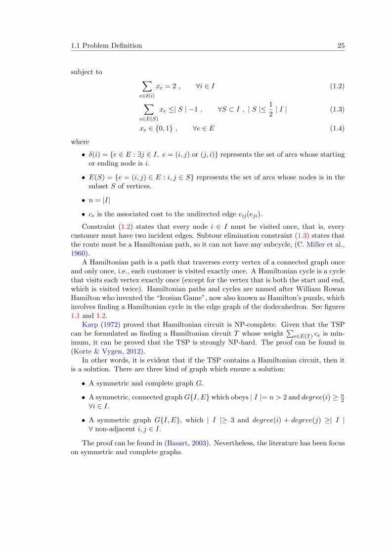
Constraint (1.2) states that every node i ∈ I must be visited once, that is, everycustomer must have two incident edges. Subtour elimination constraint (1.3) states thatthe route must be a Hamiltonian path, so it can not have any subcycle, (C. Miller et al.,1960).
A Hamiltonian path is a path that traverses every vertex of a connected graph onceand only once, i.e., each customer is visited exactly once. A Hamiltonian cycle is a cyclethat visits each vertex exactly once (except for the vertex that is both the start and end,which is visited twice). Hamiltonian paths and cycles are named after William RowanHamilton who invented the “Icosian Game”, now also known as Hamilton’s puzzle, whichinvolves finding a Hamiltonian cycle in the edge graph of the dodecahedron. See figures1.1 and 1.2.
Karp (1972) proved that Hamiltonian circuit is NP-complete. Given that the TSPcan be formulated as finding a Hamiltonian circuit T whose weight
∑e∈E(T ) ce is min-
imum, it can be proved that the TSP is strongly NP-hard. The proof can be found in(Korte & Vygen, 2012).
In other words, it is evident that if the TSP contains a Hamiltonian circuit, then itis a solution. There are three kind of graph which ensure a solution:
• A symmetric and complete graph G.
• A symmetric, connected graphG{I, E} which obeys | I |= n > 2 and degree(i) ≥ n2
∀i ∈ I.
• A symmetric graph G{I, E}, which | I |≥ 3 and degree(i) + degree(j) ≥| I |∀ non-adjacent i, j ∈ I.
The proof can be found in (Basart, 2003). Nevertheless, the literature has been focuson symmetric and complete graphs.

26 Traveling Salesman Problem
Figure 1.1: An original copy of Sir William Rowan Hamilton’s famous “Icosian Game”in The Puzzle Museum. Copyright @ 2015 The Puzzle Museum James Dalgety.
Figure 1.2: “Hamiltonian path”. Copyright under CC BY-SA 3.0 via Wikimedia Com-mons by Christoph Sommer.
1.2 Its variants
There are several variants of the Traveling Salesman Problem, the most basic instanceof the TSP is assuming that the distance cost is symmetric, i.e., the distance betweentwo customers is the same in each opposite direction forming an undirected graph. Onthe other side, the Asymmetric TSP is a generalization of the TSP which assumes thatthe distance cost is asymmetric obtaining a directed graph. Usually, in real world, TSPappears with many side constraints. Most important restrictions are:
• Every customer has to be supplied within a certain time window. This problemis called the TSP with Time Windows and also can include other time data suchas travel times between every pair of nodes, service times and a maximum tourduration. Normally, this problem considers the minimization of either the totaltime or cost of the tour.

1.2 Its variants 27
• Customers want to delivery some goods to other customer. This problem is calledthe TSP with Pick-Up and Delivery and it is defined on a graph containing pickupand delivery vertices between which there exists a one-to-one relationship, thatmeans that customers can be divided into two groups according to the type ofservice required (delivery or pick-up). The problem consists of determining a min-imum cost tour such that each pick-up vertex is visited before its correspondingdelivery customer. It can be a sequential ordering problem or a capacitated prob-lem.
• Customers may have several predecessors. This problem is called the Precedence-Constrained TSP and it is a generalization of the TSP with Pick-Up and Deliveryin which each customer may have several predecessors, i.e., another customerswhich have to been visited before the customer. Then, there exists a many-to-onerelationship.
• The salesman must first delivery goods and then pickup goods. This problem iscalled the TSP with Backhauls where an uncapacitated vehicle must visit all thedelivery customers before visiting a pickup customer. In other words, a set oflocations must be routed before the rest of locations.
• There are more than one salesman. This problem is called the Multiple TSP and itis a generalization of the TSP in which more than one salesman is allowed. Givena set of customer, the objective of the problem is to determine a tour for eachsalesman such that the total tour cost is minimized and that each city is visitedexactly once by only one salesman.
• The salesman must purchase a set of goods. This problem is called the TravelingPurchaser Problem and it deals with a purchaser who is charged with purchasingof all required products. He can purchase these products in several cities, but atdifferent prices and not all cities offer the same products. The objective is to finda route between a subset of the cities, which minimizes total cost (travel cost +purchasing cost).
• Transportation of perishable goods. This problem is called the Bottleneck TSPand it is a variation with a different objective function. It considers a weightedgraph and its objective is minimizing the weight of the most weighty edge of thecycle. Another similar problem is the Maximum Scatter TSP which is used insequencing the riveting operations when fastening sheets of metal together. Thegoal is to maximize the length of a shortest edge in the tour.
• Visiting only a subset of the customers. This problem is called the Prize CollectingTSP where each customer has an associated prize, and a salesman calls for aminimum travel cost covering a customer subset whose total prize is not less thana given value.

28 Traveling Salesman Problem
• Some values are random. The Stochastic TSP can consider that some values arerandom like travel costs, customers’ serve time or travel time, the purchased prices,the number of salesmen. Also the Dynamic TSP considers that customers can bedeleted or inserted over time.
These problems are the most significant in real world, for the interested reader seekingmore information on TSP variants or generalizations, we suggest (Gutin & Punnen,2002).
1.3 Literature Review
As it can be noticed in the following literature review, the TSP problem has been solvedmainly by exact methods and metaheuristic algorithms. The most important exactalgorithms for this problem have been developed with linear programming, Branch-and-Bound and Cutting-Plane implementation. They work reasonably fast only forsmall problem sizes. The approximation methods are classified into metaheuristic andheuristic techniques. Metaheuristics, instead of exact algorithms, are extensively usedto solve NP problems.
Dantzig et al. (1954) expressed the problem as an integer linear program and devel-oped the cutting plane method for its solution. They showed the effectiveness of theirmethod by solving a 49-city instance.
Significant progress has been made using Cutting-Planes and Branch-and-Boundtechniques as in the work of (Grotschel & Holland, 1991), (Padberg & Rinaldi, 1987),(Padberg & Rinaldi, 1991), (Radharamanan & Choi, 1986) among others. It has beenmanaged to exactly solve instances with up to 2392 cities.
One of the best-known exact method is named Concorde, a TSP Solver developedby Applegate et al. (2015), that employs an architecture that ensures the validity of thelower-bound computations using linear programming and a cutting-plane implementa-tion. Applegate et al. (2006) explains how they solved optimally a instance of 85,900locations taking over 136 CPU-years, and how they solved the World TSP of 1,904,711cities yielding a gap of only 0.0474% respect the best tour length found by Helsgaun(2009) using a variant of his LKH heuristic algorithm.
The classical heuristic methods are Nearest Neighbor, 2-Opt, and 3-Opt methods,which are frequently used for constructing and improving initial solutions in metaheuris-tics. A survey of them can be found in (Nilsson, 2003).
Lin and Kernighan (1973) proposed an effective heuristic for the TSP, which is basedon a k-Opt procedure with k variable in each step. Later, Helsgaun (2000) described animplementation even more effective of this heuristic, named LKH, for both symmetricand asymmetric problems. LKH currently holds the record for the best instances ofproblems with unknown optimal (DIMACS TSP Challenge 2002 ) with sizes rangingfrom 1,000 to 10,000,000 nodes.
Some of the latest heuristic approaches that are being well adapted to solve theNP-hard TSP are Genetic algorithm, Memetic Algorithm and Ant colony.

1.3 Literature Review 29
Genetic algorithms are population based search techniques which mimics the princi-ples of natural selection and natural genetics laid by Charles Darwin, that was proposedby Holland (1975). R. Cheng and Gen (1994) described a greedy selection crossoveroperator, which is designed for path representation and performed at gene level. It canutilize local precedence and global precedence relationship between genes to perform in-tensive search among solution space to reproduce an improved offspring. Diverse authorshave contribute to improve the Genetic algorithms since then as (Nagata & Kobayashi,2013), (Gen & Cheng, 2000), (Ray et al., 2007), (Deep & Mebrahtu, 2011), betweenothers authors.
The Memetic algorithms combine the recognized strength of population in Geneticalgorithm with the intensification capability of a local search, i.e., all agents evolvesolutions until they become local minima of a certain neighborhood, for an introductionsee (Neri et al., 2012). The method proposed by Freisleben and Merz (1996) introduces anew recombination operator, called Distance Preserving Crossover, their algorithm usesthe Lin-Kernighan heuristic as a local search engine for the Euclidean instances. Someof the latest publications in the field are (Bontoux et al., 2010), (Y. Wang et al., 2011),(Osaba & Dıaz, 2012), and (Gutin & Karapetyan, 2010).
Regarding the Ant Colony approach, the natural metaphor on which it is based onhow real ants are capable of finding the shortest path from a food source to their nestwithout using visual clues by exploiting pheromone information, initially proposed byDorigo and Gambardella (1997). Some of the most prominent authors are (Dorigo &Gambardella, 2014), (S. M. Chen & Chien, 2011), (Karaboga & Gorkemli, 2011), and(Uchida et al., 2012).
In order to know about the closeness of the upper bound to the optimum value, onemust also know a lower bound on the optimum value. Several relaxations have beenconsidered for the TSP, such as the n-path relaxation, the assignment relaxation, the2-matching relaxation, the 1-tree relaxation, and the linear programming relaxation.
For the interested reader seeking more information on this important problem, wesuggest the seminal paper on the problem by Dantzig et al. (1954) and the books byLawler et al. (1985) and by Reinelt (1994). For a survey of its variations, see (Gutin &Punnen, 2002). For a deep understanding of how algorithms for TSP work, see the bookby Applegate et al. (2006), which besides providing a wide overview on TSP historyand on its applications. For a global survey that summarize most of the research andprovide extensive references, see (K. L. Hoffman et al., 2013), (Lawler et al., 1985) and(Laporte, 1992).
Lagrangian Relaxation
Finally, our interest is focused on the Lagrangian Relaxation for solving the TSP. Thereare two well known relaxations for the TSP: the 2-matching problem and the minimumspanning tree.
The first one was introduced by Balas and Christofides (1981) who relax the SubtourElimination constraint obtaining a 2-matching problem as Lagrangian relaxed problem.

30 Traveling Salesman Problem
The 2-Matching problem can be solved in polynomial time (Edmonds & Johnson, 1973),an efficient implementation can be found in Pekny and Miller (1994).
The second one was proposed by Held and Karp (1970, 1971), they relax the set ofconstraints requiring that all vertices must have two incident edges except for the depot,and the obtained relaxed problem is a minimum Weight 1-Tree which is a variant of theminimum spanning tree.
The algorithm proposed by Held and Karp (1970, 1971) was the basis for the Subgra-dient algorithm. As explained previously on page 14, the main difficulty of this algorithmlays on choosing a correct step size. Some variations concerning the choice of initial stepsizes and update of step sizes are (K. H. Hansen & Krarup, 1974), (Smith & Thompson,1977), (Volgenant & Jonker, 1982), and (Balas & Toth, 1985). Make a special attentionto Zamani and Lau (2010), who presents an effective procedure that finds lower boundsfor the TSP based on the 1-Tree using a learning-based Lagrangian relaxation technique.The procedure can dynamically alter its step size depending upon its previous iterations,thus achieves better convergence.
An analysis of the Lagrangian relaxation introduced by Held and Karp (1970) canbe found in Shmoys and Williamson (1990). Smith et al. (1990) analyze the Lagrangianrelaxation introduced by Balas and Christofides (1981) and conclude that the lowerbounds are a bit worse.
Extensive research has been devoted to Lagrangian heuristic, which combines aheuristic with the Lagrangian Relaxation. Fisher (2004) discusses of some early ex-amples of Lagrangian heuristics for the Generalized Assignment problem. Barahona andAnbil (2000) present the Volume algorithm, that is an extension to the Subgradient al-gorithm to produce primal as well as dual solutions. They present successful experiencefor the Set Partitioning, the Set Covering, the Max-Cut and the Plant Location.
Respect to the TSP, the most relevant authors extending LR are: Christofides (1976)whose algorithm first finds a minimum cost spanning tree, then finds the minimum costEulerian augmentation of that tree, and finally shortcuts the corresponding Eulerianwalk into a tour; Timsjo (1999) presents a solution strategy based on the Lagrangianrelaxation of the 1-Tree for the TSP and using a Subgradient algorithm. The authorapplies a heuristic to modify the relaxed solution into a feasible primal one; In the workof Volgenant and Jonker (1982), it is proposed a Branch-and-Bound algorithm for theTSP based on the ascent method to calculate the 1-Tree bounds, and a heuristic is usedto provide upper bounds throughout the computations; In (Belloni & Lucena, 2000), theauthors present a Lagrangian Relax-and-Cut algorithm for the TSP, where violated con-straints are attempted to be identified and are dualized for every Lagrangian relaxationproblem eventually solved. For more information on Lagrangian Relax-and-Cut algo-rithm, see (Lucena, 2006); Other prominent authors are Marinakis et al. (2005, 2009),they present a hybrid method for solving the TSP proposing a combination of genetic al-gorithms, GRASP and LR. Constraints requiring that each node has two incident edgesare relaxed obtaining a minimum spanning tree as the Lagrangian dual problem.

1.4 Lagrangian Dual Problem 31
1.4 Lagrangian Dual Problem
The proposed LR uses the relaxation proposed by Held and Karp (1971) which relaxesthe constraint set (1.2) requiring that all customers must be served expect for the depot(i = 1). Therefore, the obtained relaxed problem is a Minimum Weight 1-Tree.
A minimum weight 1-Tree consists of a Spanning Tree of minimal total length on thenode set I r {1} combined with the shortest two edges incident to node 1 (depot). Aspanning tree of a graph is just a subgraph that contains all the vertices and it forms atree that is an undirected graph in which any two vertices are connected by exactly onepath.
The Lagrangian Dual problem obtained relaxing the constraint set (1.2) is as follows:
maxu∈Rn
L(u) (1.5)
where:
L(u) = minx 1−Tree
∑e∈E
cexe +∑i∈I
ui(2−∑e∈δ(i)
xe) (1.6)
it weight the relaxed constraints with a multiplier vector u of appropriate dimension andunrestricted sign, defining the subgradient γki = 2−
∑e∈δ(i) xe.
Indeed, all subcycles can be avoided constructing the solution x as a 1-Tree, and afeasible solution of the TSP is a 1-Tree having two incident edges at each node (Held &Karp, 1971). The main advantage of this approach is that relaxing the set constraint1.2, at the same time, it avoids the set of subtour elimination constraints (1.3) whichcontains an exponential number of constraints.
Furthermore, finding a minimum 1-Tree is relatively easy (Cormen et al., 2001).Prim’s Algorithm and Kruskal’s Algorithm are two algorithms commonly used for findinga minimum spanning tree.
Prim’s Algorithm
An algorithm for solving the minimum weighted 1-Tree is Prim’s algorithm, which wasdeveloped by Jarnik in 1930 and rediscovered by Prim in 1957 and Dijkstra in 1959.
Prim’s Algorithm continuously increase the size of a tree starting with a single ar-bitrary vertex until it spans all the vertices. In each iteration it chooses the minimalweighted edge where one of its vertex has already been visited but the other has notbeen, given that, each pair of vertices must be connected by exactly one path. Its timecomplexity is O(n2), where n is the number of vertices.
Given a complete undirected graph G = (I, E) representing the TSP, where I rep-resent the set of nodes (customers and depot) and E = {(i, j) : i, j ∈ I} the set ofundirected edges. Let be the set of customers I ′ = {2, ..., n} and their correspondingedges E′ ⊂ E.
The Algorithm 2 shows the Prim’s Algorithm for the 1-Tree. Remember that the socalled 1-Tree is a tree and therefore, it has to be added two edges incidents to the depot(i = 1).

32 Traveling Salesman Problem
Algorithm 2 Prim’s Algorithm for the 1-Tree
Initialization:Find e = (i, j) ∈ E′ the minimal weighted edge.Initialize T = {e} the tree.Initialize V = {i, j} the set of visited nodes.
while V 6= I ′ doFind e = (i, j) ∈ E′ the minimal weighted edge with a visited node, i ∈ V , and anunvisited node, j ∈ I ′ r V .Add this edge to the tree: T = T ∪ {e}.Add the unvisited node: V = V ∪ {j}.
end while
Find e = (1, i) ∈ E the minimal weighted edge connected to the depot.Add this edge to the tree: T = T ∪ {e}.Find e = (1, j) ∈ E the second minimal weighted edge, i.e., j 6= i.Add this edge to the tree: T = T ∪ {e}.return T .
1.5 An Experiment in Convergence
The purpose of this section is to show the importance of the step size on the Subgradientalgorithm. An easy problem has been chosen to demonstrate its important, the SpanishAirports problem which requires visiting once each of the 37 airports of Spain, see An-nex Appendix A. The travel distance has been obtained applying the Euclidean distancefrom the GPS coordinates, rounding it by integer values. Solving the problem 1.1 usingthe software IBMr ILOGr CPLEXr Optimization Studio (2015), its optimal value isL∗ = 7223, however, using the Nearest Neighbor Heuristic, it is found an upper boundof value UB = 8188.
In order to compare the performance of the step size, the Subgradient algorithm isapplied to the model of the Lagrangian relaxation of the TSP, see section 1.4. Figure 1.3shows the convergence of the different step sizes for the Spanish Airports problem.
Fig. 1.3a shows convergence using the next three steps sizes. It should be noticedthat despite initial perturbations the step size c) leads much faster convergence than theother steps.
a) λk = 1k . This holds because
∑k λk →∞, and λk → 0 as k →∞.
b) λk = δ{k−N} ·ρ for parameters δ0 = 2 and ρ = 0.95. This holds because the parameterδk is reduced every N iterations.
c) λk = δkUB−L(uk)‖γk‖2
and the parameter δk is reducing by ρ = 0.95 every N consecutive
iterations without improving the lower bound with δ0 = 2. This holds if the parameterUB is tight upper bound.

1.6 Tailored Lagrangian Metaheuristic 33
0 20 40 60 80 100 120 140 160 180 200−4000
−2000
0
2000
4000
6000
8000
iteration (k)
L(uk)
L* = 7223
a) λk=1/k
b) λk := δk = δk−N ρ
c) λk =δk (UB−Lk) / ||γk||2
(a) Rules a, b, and c.
0 20 40 60 80 100 120 140 160 180 200−4000
−2000
0
2000
4000
6000
8000
10000
iteration (k)
L(uk)
L* = 7223
c) λk = δk (L*−Lk) / ||γk||2
UB = 8188
c) λk =δk (UB−Lk) / ||γk||2
(b) Rule c using an upper bound or the optimal value
Figure 1.3: Convergence of the Subgradient Algorithm with different step sizes for Span-ish Airports problem.
Fig. 1.3b shows the convergence of the step size c) using different values. UsingUB = 8188, the gap between the best Lagrangian value and the optimal value is of 5%at the iteration k = 200. However, using the optimal value L∗ = 7223, it leads muchfaster convergence and finds an optimal solution at the iteration k = 104.
1.6 Tailored Lagrangian Metaheuristic
Due to the wide range of applications and the complexity of the TSP problem, innovativeand efficient algorithms are needed. Therefore, we propose a metaheuristic methodologybased on the Lagrangian Relaxation to solve the TSP. A metaheuristic “refers to amaster strategy that guides and modifies other heuristics to produce solutions beyondthose that are normally generated in a quest for local optimality” (Glover & Laguna,1997).
Our Lagrangian metaheuristic uses the Subgradient optimization algorithm com-

34 Traveling Salesman Problem
bined with a heuristic which obtains a primal feasible solution from the dual variable.Compared with classical heuristics, our Lagrangian Metaheuristic provides both an up-per and a lower bounds (UB and LB), and a posteriori quality check of the solution isobtained.
The main contribution of our method is that it has been introduced a parameter toimprove the algorithm convergence on the optimal solution. That parameter is improvedwithin the same process using the upper bound (UB) of the primal solutions obtainedby the heuristic.
Our Tailored Lagrangian Metaheuristic metaheuristic in detail
Our proposed TLM metaheuristic is shown in Algorithm 3. A heuristic obtains a feasiblesolution from the dual variable, so it tries to improve the UB and hence, a betterconvergence using rule (c) is obtained. Eventually, the best of these feasible primalsolutions may be provided if the method is stopped.
An optimal solution will be found if the method reaches γki = 0, i.e., the 1-Tree isa Hamiltonian cycle. Since we are interested in developing a methodology applicable toreal problems where the computational time to solve instance is limited, it is added twostopping criteria based on the maximum number of iterations (k < maxiterations) andon a floating-point exception (step-size λk < 10−15), see line 5.
The proposed metaheuristic uses the Nearest Neighbor Heuristic to obtain an initialvalue of the Upper Bound in line 3. This heuristic is one of the most commonly usedto find UB, since that is easy to implement and it is computationally efficient, (Lin &Kernighan, 1973).
In line 6, Prim’s algorithm is used to solve the Lagrangian Dual Problem of the TSP,as explained in section 1.4. Then, the subgradient is calculated in line 7, if its values are0, the optimal solution is found and the iterative procedure is stopped in line 10.
The Proposed Heuristic
The proposed heuristic to improve the UB is applied when the 1-Tree is nearly a Hamil-tonian cycle, that is when the subgradient satisfies ‖ γk ‖2< ξ, see lines 11-12.
A parameter ξ is used to determine when to apply the heuristic, in line 11. A goodestimation of the parameter ξ would avoid increasing the computation time excessively.First, its value may be large, for instance the value of the first iteration, ξ = ‖ γ1 ‖2,but it should be updated whenever a better feasible solution is found according toξ =‖ γk ‖2. Eventually, the heuristic could find the optimal solution without detectingit, so the method would continue iterating until LB = UB.
As any solution is a 1-Tree, this criterion means that the solution has few verticeswithout two incident edges. This heuristic replaces an edge e = (i, j) where j has someextra edges (i.e., γkj < 0) for an edge e = (i, l) where vertex l has one single edge (i.e.,
γkl = 1) minimizing the cost of the exchange.
In the presented approach, two different moves have been defined (Figure 1.4): (a)unlimited move respect the vertices, and (b) limited move only replaces edges which

1.6 Tailored Lagrangian Metaheuristic 35
Algorithm 3 Tailored LR-based method for the TSP
1: Initialization:2: Initialize parameters δ0 = 2; ρ = 0.95;αL = 1/3;L = 03: Obtain an UB applying Nearest Neighbour Heuristic4: Initialize multiplier u0 = 05: while k < maxiterations or λk < 10−15 do6: Solve the Lagrangian dual problem L(uk) with optimal solution xk
7: Update the subgradient γki = 2−∑e∈δ(i)
xke
8: Check the subgradient:9: if ‖ γk ‖2= 0 then
10: An optimal solution is found → Exit11: else if ‖ γk ‖2< ξ then12: Apply a heuristic to improve the UB13: end if14: Check the parameter L:15: if L(uk) > L then16: It is updated, L = L(uk) + αL(UB − L(uk))17: end if18: if L > UB then19: L = UB20: end if21: Update the parameter δk:22: if L(uk) < LB then23: δk+1 = δkρ24: else25: LB = L(uk)26: δk+1 = δk
3−ρ2
27: end if
28: Update the step size λk = δkL− L(uk)
‖ γk ‖229: Update the Lagrangian multiplier uk+1 = uk + λkγ
k
30: k ← k + 131: end while

36 Traveling Salesman Problem
i
j2
l
j
i
j2
l
j
(a) The unlimited move
i
lj
i
lj
(b) The limited move
Figure 1.4: Movements of the proposed heuristic: swapping elj for eil
both vertices i and l are connected to same vertex j. Our proposed heuristic is shownin Algorithm 4.
First, it iteratively applies the unlimited movement but being aware that it coulddivide the 1-Tree into disconnected trees. For each i with γki = 1, it swaps edge elj foreil minimize the cost of the exchange:
{i, j, l} = argmin{cil − clj | γki = 1, γkj < 0, γkl ≥ 0, (l, j) ∈ T k and (i, l) ∈ E r T k
}(1.7)
Then, it iteratively applies the limited movement until it is found a feasible solution.For each pair {i, j} where γki = 1 and j is the first connected node with γkj < 0, it selectsthe neighbor l minimizing the cost of the exchange (1.7).
Convergence: new parameter L
As mentioned, algorithm’s convergence is critically influenced by the step-size λk. Usingrule (c) explained on page 15, this value relies on either the LB or the UB, which arenormally unknown or bad estimated. Therefore, convergence may not be assured forall cases. In order to overcome this limitations, we propose the use of a parameter L,such that LB ≤ L ≤ UB. By definition, this new parameter corresponds to a betterestimation of the optimal value L∗ than those obtained for LB and UB. The calculationof the step-size turns into (see line 28):
λk = δkL− L(uk)
‖ γk ‖2
Convergence is guaranteed if the term L−L(uk) tends to zero. In turn, convergenceefficiency can be improved as long as the new L parameter gets closer to the (unknown)optimal solution. The main idea is very simple: as the algorithm converges to thesolution, new better lower bounds are known and new better upper bounds estimationscan be obtained by using the heuristic designed to get feasible solutions. Therefore, inlines 14-20, the parameter L is updated according to the following conditions:

1.6 Tailored Lagrangian Metaheuristic 37
Algorithm 4 Heuristic to obtain feasible solution for a 1-Tree
Data: T k the obtained 1-TreeInitialize:
V + = {i ∈ I | γki = 1} the subset of vertices which only has one edgeV − = {j ∈ I | γkj < 0} the subset of vertices which has more than two edge
Unlimited Movement:do ‖ V + ‖ times
{i, j, l} = argmin{cil−clj | i ∈ V +, j ∈ V −, γkl ≥ 0, (l, j) ∈ T k and (i, l) ∈ ErT k
}if nodes l and j are connected in T k r (l, j) ∪ (i, l) then
Swap these edges within the tree: T k = T k r (l, j) ∪ (i, l)Update node i: γki = 0 and V + = V + r {i}Calculate γkjif γkj = 0 then
Update node j: V − = V − r {j}end if
end ifend do
Limited Movement:do ‖ V + ‖ times
Find {i, j, l} = argmin{cil − clj | γkl ≥ 0, (l, j) ∈ T k and (i, l) ∈ E r T k
}where
i ∈ V +, the node j is the nearest node of V − connected to i, and l is a neighborof j but not in the path i, j
Swap these edges within the tree: T k = T k r (l, j) ∪ (i, l)Update node i: γki = 0 and V + = V + r {i}Calculate γkjif γkj = 0 then
Update node j: V − = V − r {j}end if
end doreturn T k.
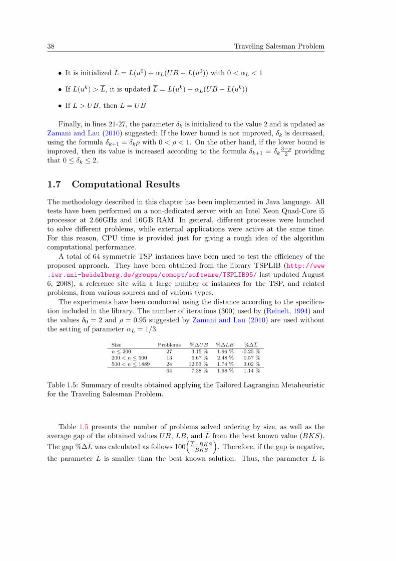
38 Traveling Salesman Problem
• It is initialized L = L(u0) + αL(UB − L(u0)) with 0 < αL < 1
• If L(uk) > L, it is updated L = L(uk) + αL(UB − L(uk))
• If L > UB, then L = UB
Finally, in lines 21-27, the parameter δk is initialized to the value 2 and is updated asZamani and Lau (2010) suggested: If the lower bound is not improved, δk is decreased,using the formula δk+1 = δkρ with 0 < ρ < 1. On the other hand, if the lower bound isimproved, then its value is increased according to the formula δk+1 = δk
3−ρ2 providing
that 0 ≤ δk ≤ 2.
1.7 Computational Results
The methodology described in this chapter has been implemented in Java language. Alltests have been performed on a non-dedicated server with an Intel Xeon Quad-Core i5processor at 2.66GHz and 16GB RAM. In general, different processes were launchedto solve different problems, while external applications were active at the same time.For this reason, CPU time is provided just for giving a rough idea of the algorithmcomputational performance.
A total of 64 symmetric TSP instances have been used to test the efficiency of theproposed approach. They have been obtained from the library TSPLIB (http://www.iwr.uni-heidelberg.de/groups/comopt/software/TSPLIB95/ last updated August6, 2008), a reference site with a large number of instances for the TSP, and relatedproblems, from various sources and of various types.
The experiments have been conducted using the distance according to the specifica-tion included in the library. The number of iterations (300) used by (Reinelt, 1994) andthe values δ0 = 2 and ρ = 0.95 suggested by Zamani and Lau (2010) are used withoutthe setting of parameter αL = 1/3.
Size Problems %∆UB %∆LB %∆Ln ≤ 200 27 3.15 % 1.96 % -0.25 %200 < n ≤ 500 13 6.67 % 2.48 % 0.57 %500 < n ≤ 1889 24 12.53 % 1.74 % 3.02 %
64 7.38 % 1.98 % 1.14 %
Table 1.5: Summary of results obtained applying the Tailored Lagrangian Metaheuristicfor the Traveling Salesman Problem.
Table 1.5 presents the number of problems solved ordering by size, as well as theaverage gap of the obtained values UB, LB, and L from the best known value (BKS).
The gap %∆L was calculated as follows 100(L−BKSBKS
). Therefore, if the gap is negative,
the parameter L is smaller than the best known solution. Thus, the parameter L is

1.7 Computational Results 39
Problem BKS UB %∆UB LB %∆LB CPUtime (s)eil51 426 440 3.29 % 422.42 0.84 % 0.226st70 675 687 1.78 % 670.89 0.61 % 0.255eil76 538 544 1.12 % 536.94 0.20 % 0.297pr76 108159 108584 0.39 % 105112.85 2.82 % 0.250rat99 1211 1237 2.15 % 1205.91 0.42 % 0.257kroA100 21282 21319 0.17 % 20930.10 1.65 % 0.432kroB100 22141 22931 3.57 % 21830.02 1.40 % 0.267kroC100 20749 21270 2.51 % 20467.78 1.36 % 0.530kroD100 21294 21792 2.34 % 21138.27 0.73 % 0.298kroE100 22068 22905 3.79 % 21798.00 1.22 % 0.734rd100 7910 8006 1.21 % 7898.65 0.14 % 0.499eil101 629 629 0.00% 627.35 0.26 % 0.360lin105 14379 14402 0.16 % 14370.14 0.06 % 0.237pr107 44303 44420 0.26 % 39313.79 11.26 % 0.379pr124 59030 60112 1.83 % 58048.18 1.66 % 0.463bier127 118282 124502 5.26 % 117396.83 0.75 % 1.404ch130 6110 6203 1.52 % 6074.46 0.58 % 0.351pr136 96772 102534 5.95 % 95373.05 1.45 % 0.905ch150 6528 6640 1.72 % 6488.12 0.61 % 1.279kroA150 26524 27598 4.05 % 26280.90 0.92 % 1.608kroB150 26130 27273 4.37 % 25725.39 1.55 % 1.577pr152 73682 78848 7.01 % 66583.97 9.63 % 0.219u159 42080 42636 1.32 % 41921.90 0.38 % 1.186rat195 2323 2489 7.15 % 2290.58 1.40 % 2.443d198 15780 17500 10.90 % 14372.36 8.92 % 3.093kroA200 29368 30983 5.50 % 29056.19 1.06 % 3.231kroB200 29437 31126 5.74 % 29158.27 0.95 % 2.960ts225 126643 144299 13.94 % 115472.09 8.82 % 1.145tsp225 3919 4261 8.73 % 3875.89 1.10 % 3.230pr226 80369 84203 4.77 % 78451.35 2.39 % 3.155gil262 2378 2473 3.99 % 2354.00 1.01 % 5.117pr264 49135 50868 3.53 % 46236.48 5.90 % 5.180a280 2579 2704 4.85 % 2565.40 0.53 % 7.202pr299 48191 51053 5.94 % 47360.81 1.72 % 7.860lin318 42029 45017 7.11 % 41768.56 0.62 % 5.695rd400 15281 16061 5.10 % 15147.55 0.87 % 17.276fl417 11861 13137 10.76 % 11144.00 6.05 % 12.179pr439 107217 112768 5.18 % 105306.76 1.78 % 11.249pcb442 50778 53840 6.03 % 50456.63 0.63 % 16.069d493 35002 37397 6.84 % 34721.01 0.80 % 35.550u574 36905 38985 5.64 % 36690.41 0.58 % 35.381rat575 6773 7317 8.03 % 6718.70 0.80 % 44.725p654 34643 43638 25.96 % 32487.42 6.22 % 3.858d657 48912 52985 8.33 % 48420.58 1.00 % 115.474u724 41910 46883 11.87 % 41618.86 0.69 % 160.662rat783 8806 9674 9.86 % 8766.59 0.45 % 132.460pr1002 259045 283008 9.25 % 256272.34 1.07 % 252.525u1060 224094 250775 11.91 % 221469.74 1.17 % 411.675vm1084 239297 265714 11.04 % 235787.50 1.47 % 294.671pcb1173 56892 63499 11.61 % 56276.66 1.08 % 617.5433d1291 50801 56274 10.77 % 49872.37 1.83 % 415.448rl1304 252948 269195 6.42 % 248809.85 1.64 % 492.303rl1323 270199 297319 10.04 % 265325.26 1.80 % 245.389nrw1379 56638 64474 13.84 % 56284.49 0.62 % 1185.057fl1400 20127 23358 16.05 % 19089.32 5.16 % 2968.874u1432 152970 176933 15.67 % 152031.82 0.61 % 619.392fl1577 22249 25631 15.20 % 20661.34 7.14 % 710.379d1655 62128 69956 12.60 % 61177.18 1.53 % 1941.611vm1748 336556 381719 13.42 % 331209.14 1.59 % 1456.419u1817 57201 64062 11.99 % 56583.97 1.08 % 2465.488rl1889 316536 351197 10.95 % 310987.88 1.75 % 1820.504u2152 64253 73443 14.30 % 63753.38 0.78 % 1135.083u2319 234256 283523 21.03 % 233605.99 0.28 % 18698.743pr2392 378032 434652 14.98 % 372679.05 1.42 % 5759.861
Table 1.6: Results obtained applying the Tailored Lagrangian Metaheuristic for theTraveling Salesman Problem

40 Traveling Salesman Problem
0 50 100 150 200 250 30013.000
14.000
15.000
16.000
17.000
18.000
19.000
20.000
21.000
Iterations
Tota
l Tra
vel D
ista
nce
lin105
LB
L
UB
(a) Problem lin105
0 50 100 150 200 250 30013.000
14.000
15.000
16.000
17.000
18.000
19.000
20.000
Iterations
Tota
l Tra
vel D
ista
nce
rd400
LB
L
UB
(b) Problem rd400
0 50 100 150 200 250 30090.000
95.000
100.000
105.000
110.000
115.000
120.000
125.000
130.000
135.000
Iterations
Tota
l Tra
vel D
ista
nce
pr439
LB
L
UB
(c) Problem pr439
Figure 1.7: Convergence of LB, L, and UB in some problems.

1.8 Conclusions 41
a good estimation with regard to an unknown lower bound or an initial upper boundobtained with a Nearest Neighbor Heuristic.
Table 1.6 presents results of a total of 64 instances comparing the results obtainedto best known solution (BKS). The columns shows: UB best feasible value, %∆UB per-centage distance from BKS of the UB, LB best dual value, %∆LB percentage distancefrom BKS of the LB, and tFinal final CPU time in seconds.
Figure 1.7 shows the evolution of upper and lower bounds on three runs. As it can beseen, the parameter L is updated according to the previous conditions explained, and itshould be noticed that UB is improved every time the proposed heuristic finds a bettervalue. The figure shows how LB, L, and UB converge on BKS.
For the lin105 problem in Figure 1.7a, it has a quickly convergence in the first 100 iter-ations, however, it does not reach the optimal. The initial UB obtained with the NearestNeighbor heuristic has a gap of 41.57%, our Lagrangian methodology dramatically im-proves this value up to 8.84% only in the second iteration. It shows the convergenceof UB, LB and our parameter L with theirs final respective gaps of 0.16%, 0.06% and0.16%.
Figure 1.7b shows rd400 problem, the initial UB obtained with the Nearest Neighborheuristic has a gap of 26.06%, it shows the convergence of UB, LB and our parameterL with theirs final respective gaps of 5.10%, 0.87% and 1.03%.
For the pr439 problem in Figure 1.7c, the initial UB obtained with the NearestNeighbor heuristic has a gap of 24.20%, it shows the convergence of UB, LB and ourparameter L with theirs final respective gaps of 5.18%, 1.78% and 0.36%.
1.8 Conclusions
This chapter has presented a metaheuristic methodology based on the Lagrangian Relax-ation technique. This scheme has been used to tackle the Traveling Salesman Problem,showing very good results both in terms of the quality of the solution and in terms ofcomputational efficiency.
Our proposed Tailored Lagrangian Metaheuristic method uses the Subgradient algo-rithm combined with a heuristic. The motivation of our method is the common sensebelief that dual solutions must obviously be relevant to primal solutions. The proposedheuristic is introduced in order to obtain a feasible solution from the dual variable pro-viding both UB and LB, thus an a posterior quality check of the solution is obtained.
A new parameter L which is updated using the values of both UB and LB hasimproved significantly algorithm’s convergence on the optimal solution.
In spite of optimality can not be always reached, the proposed method is able toprovide a feasible solution with a tight gap between the primal and the optimal cost ina reasonable number of iterations.


Chapter 2
Capacitated Vehicle RoutingProblem
This chapter presents an application of the Tailored Lagrangian Metaheuristic (TLM)proposed in Section 1.6. It presents an original hybrid approach to solve the Capaci-tated Vehicle Routing Problem (CVRP). The approach proposes a Multi-Start VariableNeighborhood Descent (VND) (P. Hansen & Mladenovic, 2003) structure whose localsearch process is supported by Constraint Programming (CP) (Rossi et al., 2006) andour TLM.
On the one side, our metaheuristic is used to efficiently find the optimal routingsolution for each transportation resource. On the other side, using the CP paradigmprovides the required flexibility to model those operational constraints, beyond vehiclecapacity, that are usually present in most real application cases. Due to this approach,adding these constraints is just a constraint modeling issue, i.e., no change on the solvingstrategy is required to deal with more realistic problems.
A probabilistic (Randomized) Clarke and Wright Savings (RCWS) (Juan et al., 2011)constructive method is used to generate initial solutions. This algorithm provides differ-ent good quality solutions that are used as seeds to launch the exploration of differentregions of the search space. Therefore, the RCWS probabilistic behavior introduces anatural diversification mechanism and turns the scheme into an approach likely to beparallelized.
The CVRP has been selected mainly because there are huge amounts of models,techniques, benchmarks, and research on this topic. Hence, the proposed methodologycan be easily compared —in terms of computational efficiency and solution quality—with previously existing approaches. Nevertheless, from the perspective of its industrialapplicability, the basic CVRP model can be extended to tackle different realistic cases bymeans of the proposed optimization scheme. These cases include operational constraintsbeyond the basic vehicle capacity. Affordable examples are limitations on the totaldriving time of each route, incompatible customer-driver associations or constraints onthe customer visiting periods (e.g., customer forbidden visit day when building dailyroutes for a distribution problem). The proposed optimization approach, as presented
43

44 Capacitated Vehicle Routing Problem
in this chapter, is specifically designed to deal with those operational constraints thatinvolve the allocation part of the VRP.
The approach presented in this chapter was first presented in (Herrero et al., 2010a)and (Guimarans et al., 2010) where we introduced a first methodology which com-bined CP and TLM within a VNS framework. The current approach was presentedin (Guimarans et al., 2011b) and (Guimarans et al., 2013), it also integrates the RCWS-based Multi-Start approach which is significantly more efficient –both in terms of com-putational times and solutions’ quality.
2.1 Problem Definition
The Vehicle Routing Problem (VRP) provides a theoretical framework for approachingthe class of logistic problems dealing with physical distribution. This is among the mostpopular research areas in combinatorial optimization. It was first defined by Dantzigand Ramser (1959), and several variants of the basic problem have been proposed andstudied later. These variants represent different types of operational constraints suchas, for instance, time windows, pick up and delivery, heterogeneous fleets or multi-depotproblems.
The Capacitated version of the VRP (CVRP) consists of determining the optimalset of routes for a fleet of vehicles to deliver goods to a given set of customers, thereforeit is a generalization of the TSP. In the model proposed in this chapter, the CVRPhas been divided into two subproblems, concerning customers’ allocation and routingoptimization separately. The first is aimed to assign customers to vehicles fulfillingcapacity limitations. The latter is used to solve each independent route to optimality,giving the best solution for a particular allocation. Thus, routing optimization processcan be viewed as solving a set of independent symmetric TSP.
The CVRP has been chosen in order to illustrate the benefits of the proposed method-ology. The CVRP is the most basic VRP variant, which assumes a fleet of vehicles ofhomogeneous capacity housed in a single depot. The CVRP is a generalization of theTraveling Salesman Problem (TSP) and is therefore NP-hard (Savelsbergh, 1985).
The CVRP is defined over a complete graph G = {I, E}, where I = {1, 2, . . . , n} isthe node set representing clients to be served plus the depot (node 1), and E = {eij =(i, j) | i, j ∈ I} is the edge set representing connecting roads, streets, etc. Edges eij inE have an associated cost cij > 0, which is the traveling cost from node i to node j.It is usual to consider symmetric costs (i.e., cij = cji,∀i, j ∈ I). Moreover, each node iin I has a demand qi ≥ 0. A fixed fleet of m identical vehicles, each one with capacityQ� max{qi}, is available at the depot to accomplish the required delivery task.
Solving the CVRP consists of determining a set of k ≤ m routes with minimum totaltraveling cost and such that:
a) each customer is visited exactly once by a single vehicle,
b) each route starts and ends at the depot, and

2.1 Problem Definition 45
c) the total demand of the customers assigned to a route does not exceed the vehiclecapacity Q.
Therefore, a solution of a given CVRP instance is a set of k routes sharing a commonstarting and finishing node (the depot). In some cases, the fleet size is not fixed andminimizing the total number of used vehicles becomes an additional objective.
Given that our approach combines LR to optimize each individual route, and CPto quickly verify the feasibility, it is based on the classical decomposition into two sub-problems: a resource allocation problem (to fit operational constraints), and a routingproblem (to minimize the associated traveling costs).
Capacity problem
The proposed customers’ allocation subproblem uses two lists of variables. A list R ofsize n, with integer domains Ri ∈ [1..m] | i = 1, ..., n, indicates which vehicle is servingthe ith customer. Qv is a list of m variables with real domain Qv ∈ [0..Q] used to tracethe cumulative capacity at each one of the m routes. Therefore, capacity constraintsare enforced through domains definition since Qv cannot get higher values than themaximum capacity Q satisfying constraint (c).
A set of dimension m× n of binary variables B has been introduced to relate R andQv values. For each vehicle v ∈ V , a list of n binary variables Bvi | i ∈ I is defined,taking value 1 whenever customer i is assigned to vehicle v and 0 otherwise. Since eachcustomer i is visited by a single vehicle, for all values of v the binary variable Bvi cantake value 1 only once. This constraint is expressed in terms of the global constraintcardinality atmost (Beldiceanu, Carlsson, & Rampon, 2005) aiming to ensure a fasterpropagation (Bessiere, 2006).
The binary set B and allocation variables R are related through the following state-ment:
Ri = ri → Brii = 1 ∀i ∈ I (2.1)
Expression (2.1) states that the ith element of the ri list of B will have value 1whenever the ith component of R takes value ri. The global constraint cardinality atmostensures propagation so all values of Bvi v ∈ V \ ri are set to 0 automatically. Therefore,cumulative capacities can be traced simply by using the following equation:
Qv =∑i∈I
Bviqi ∀v ∈ V (2.2)
Routing Problem
The routing problem, tackled for each vehicle separately, can be viewed as a TSP in-stance. For each vehicle v, the related TSP can be considered as a complete undirectedgraph G = (Iv, Ev), connecting assigned customers Iv = {i ∈ I | Ri = v} through a setof undirected edges Ev = {(i, j) ∈ E | i, j ∈ Iv}. The solution is a path connected by

46 Capacitated Vehicle Routing Problem
edges belonging to Ev that starts and ends at the depot (i = 1) and visits all assignedcustomers. Following the mathematical formulation presented in Section 1.1, a feasiblesolution of the TSP should, by definition, also satisfy constraints (a) and (b) of theCVRP, minimizing the total travel cost of the route.
2.2 Literature Review
The Clarke and Wright’s Savings (CWS) constructive algorithm (Clarke & Wright, 1964)is probably the most cited heuristic to solve the CVRP. The CWS is an iterative methodthat starts out by considering an initial dummy solution in which each customer is servedby a dedicated vehicle. Next, the algorithm initiates an iterative process for mergingsome of the routes in the initial solution. Merging routes can improve the expensiveinitial solution so that a unique vehicle serves the nodes of the merged route. Themerging criterion is based upon the concept of savings. Roughly speaking, given a pairof nodes to be served, a savings value can be assigned to the edge connecting these twonodes. This savings value is given by the reduction in the total cost function due toserving both nodes with the same vehicle instead of using a dedicated vehicle to serveeach node -as proposed in the initial dummy solution. This way, the algorithm constructsa list of savings, one for each possible edge connecting two demanding nodes. At eachiteration of the merging process, the edge with the largest possible savings is selectedfrom the list as far as the following conditions are satisfied: the nodes defining the edgeare adjacent to the depot, and the two corresponding routes can be feasibly merged-i.e., the vehicle capacity is not exceeded after the merging. The CWS algorithm usuallyprovides relatively good solutions, especially for small and medium-size problems, but italso presents difficulties in some cases (Gaskell, 1967). Many variants and improvementsof the CWS have been proposed in the literature. For a comprehensive discussion onthe various CWS variants, the reader is referred to Toth and Vigo (2002b) and Laporte(2007).
Monte Carlo Simulation (MCS) can be defined as a set of techniques that make useof random numbers and statistical distributions to solve certain stochastic and deter-ministic problems (Law, 2007). MCS has proved to be extremely useful for obtainingnumerical solutions to complex problems that cannot be efficiently solved by using an-alytical approaches. Buxey (1979) was probably the first author to combine MCS withthe CWS algorithm to develop a procedure for the CVRP. This method was revisitedby Faulin and Juan (2008), who introduced an entropy function to guide the randomselection of nodes. MCS has also been used by Fernandez et al. (2000), Juan et al.(2008), Faulin et al. (2008) and Juan et al. (2009) to solve the CVRP. In this last paper,the authors make use of MCS to develop an efficient randomized version of the CWSheuristic, which we use in our approach to efficiently generate initial solutions.
Another way to address the VRP has been the use of complete methods, which ensurenot only to find the solution but also, to prove its optimality. The main drawback of thesetechniques is that they may only deal with small instances, up to 100 customers (Cordeauet al., 2007). Numerous heuristics (like the ones mentioned above) and metaheuristics
2.3 Technologies used 47
have also been studied for different VRP variants. In most cases, these methods maysolve larger instances but loosing optimality guarantees.
Using constructive heuristics as a basis, metaheuristics became popular for the VRPduring the nineties. Some early examples are the Tabu Route method by Gendreau etal. (1994) or the Boneroute method of Tarantilis and Kiranoudis (2002). Tabu searchalgorithms, like those proposed by Taillard (1993) or Toth and Vigo (2003) are amongthe most cited metaheuristics. Genetic algorithms have also played a major role inthe development of effective approaches for the VRP. Some examples are the studies ofBerger and Barkaoui (2003), Prins (2004), Mester and Braysy (2007) or Nagata (2007).Another important approach to the VRP is given by the Greedy Randomized AdaptiveSearch Procedure or GRASP (Feo & Resende, 1995; Resende, 2008; Festa & Resende,2009). A GRASP algorithm is a multi-start or iterative process in which each GRASPiteration consists of two phases: a construction phase —in which a feasible solution isproduced— and a local search phase —in which a local optimum in the neighborhoodof the constructed solution is sought. The best overall solution is kept as the result.In the construction phase, a feasible solution is iteratively constructed, one element ata time. At each construction iteration, the choice of the next element to be added isdetermined by ordering all candidate elements in a candidate list according to a greedyfunction. This function measures the (myopic) benefit of selecting each element. Theheuristic is adaptive because the benefits associated with every element are updated ateach iteration of the construction phase to reflect the changes brought on by the selectionof the previous element. The probabilistic component of a GRASP is characterized bythe random choice of one of the best candidates in the list, but not necessarily the topcandidate. This choice technique allows for different solutions to be obtained at eachGRASP iteration.
Among metaheuristics, Variable Neighborhood Search (VNS), introduced for thefirst time by Mladenovic and Hansen (1997), is a quite recent method with far lessapplication examples in VRP research. However, interesting results have been obtainedeven applying the simplest VNS algorithms, e.g., (Hasle & Kloster, 2007). EmbeddingCP and LR approaches into a general VNS framework has also demonstrated to be aneffective yet slow method to solve medium and large instances (Guimarans et al., 2011a).Combining these techniques provided a methodology able to reach good quality resultsand even to overcome some best-known solutions. However, the computational efficiencyof this methodology is far from state-of-the-art algorithms and becomes an importantissue to be addressed.
2.3 Technologies used
In this chapter we present a hybrid approach combining a randomized version of theCWS savings heuristic, the VNS metaheuristic, CP, and LR. Our approach aims atbeing an efficient procedure for obtaining quasi-optimal solutions in small- and medium-size CVRP instances and, at the same time, offers some additional advantages over otherexisting metaheuristics, namely: (a) it is a robust and flexible methodology that can be

48 Capacitated Vehicle Routing Problem
easily adapted to consider additional constraints and costs; (b) it is able to generate aset of alternative good solutions in a reasonable time period; and (c) it can be easilyexecuted in parallel.
This work has been published in Guimarans et al. (2011b), it is related to the PhDThesis of Guimarans (2012) and a previous version can be found in Herrero et al. (2010a).
Our presented approach is much more competitive with state-of-the-art metaheuris-tics. Its efficiency has been significantly enhanced by including a multi-start procedurewhich makes use of a randomized CWS heuristic in order to quickly provide a set ofdifferent “good” initial solutions, over which a flexible local-search process is applied.Thus, the VNS diversification procedure is substituted by a multi-start approach, wheredifferent regions are explored thanks to the diversity of solutions provided by the ran-domized CWS algorithm. The local search process has also been enhanced with respectto the previous work by incorporating new data structures, which permit reducing thecomputational complexity. Finally, the methodology described in the present work hasbeen parallelized to improve its efficiency.
Remember that our Tailored Lagrangian Metaheuristic is explained in Section 1.6,let us introduced the other used technologies in this approach.
Probabilistic Clarke and Wright Savings Algorithm
As discussed in Section 2.2, in the classic CWS algorithm, the edge with the largestpossible savings is selected from the list at each iteration of the merging process, as faras the following conditions are satisfied: (a) the nodes defining the edge are adjacentto the depot, and (b) the two corresponding routes can be feasibly merged -i.e., thevehicle capacity is not exceeded. The approach presented in Juan et al. (2010), instead,assigns a selection probability to each edge in the savings list. This probability shouldbe coherent with the savings value associated with each edge, i.e., edges with largersavings will be more likely to be selected from the list than those with smaller savings.In addition, this approach adds this biased random behavior without introducing toomany parameters in the algorithm. Basically, different geometric statistical distributionsduring the randomized CWS solution-construction process are employed: every time anew edge is selected from the list of available edges, a value α is randomly selectedfrom a uniform distribution in (a, b), where 0 < a ≤ b < 1. The α parameter definesthe specific geometric distribution that will be used to assign exponentially diminishingprobabilities to each eligible edge according to its position inside the sorted savings list.This way, edges with higher savings values are always more likely to be selected from thelist, but the exact probabilities assigned are variable and they depend on the concretedistribution selected at each step.
Constraint Programming
CP is a powerful paradigm for representing and solving a wide range of combinatorialproblems. Problems are expressed in terms of three entities: variables, their correspond-ing domains and constraints relating them. The problems can then be solved using

2.4 The methodology in detail 49
complete techniques such as depth-first search for satisfaction and branch and boundfor optimization, or even tailored search methods for specific problems. Rossi et al.(2006) present a complete overview of CP modeling techniques, algorithms, tools, andapplications.
Variable Neighborhood Search
A general VNS, as explained in (P. Hansen & Mladenovic, 2003), is a recent metaheuristicwhich exploits systematically the idea of neighborhood change. The Variable Neighbor-hood Descent (VND) method starts from an initial solution x′ and it is improved by alocal search process.
The local search process for each neighborhood N(x′) of x′ performs an exhaustiveexploration. All improving movements are recorded and sorted, so the best neighborx′′ ∈ N(x′) is constructed applying all independent changes in descending order. Thisway, solution values are improved faster than applying single movements.
If this neighbor is better than the incumbent, the current solution is updated andneighborhoods’ exploration is restarted. Otherwise, the algorithm keeps x′ as the bestsolution found so far and continues exploring the next neighborhood. When the VNDprocess reaches a local optimum, no solution improvement may be found according todefined neighborhoods.
Multi-Start Strategy
The VND-based local search process requires some type of diversification in order to over-come local optimality. Many techniques have been suggested to avoid getting trappedinto a local optimum and aspire to find a global one. Among others, one possibleway to achieve diversification is using a shaking mechanism within the VNS procedure.However, as more constraints are introduced in the problem, it usually becomes moreefficient -in terms of computational time employed- to generate new feasible solutionsfrom scratch than to apply complex shaking processes that might end in non-feasiblesolutions. This is especially certain if we consider that the Randomized version of theCWS used in this paper is a really fast method for generating different feasible and goodsolutions that can serve as initial solutions in our multi-start approach.
Thus, the Multi-Start strategy provides an appropriate framework which achievesdiversification by re-starting the search from a new solution once a region has beenextensively explored. Notice that each iteration includes two phases: a first one in whicha new feasible solution is constructed, and a second one in which the initial solution isimproved through a local search process.
2.4 The methodology in detail
The CVRP problem has been tackled using a RCWS-based Multi-Start approach. As ithas been previously discussed, this strategy allows to ensure an efficient diversification

50 Capacitated Vehicle Routing Problem
of the search space in order to: (a) avoid local minima, and (b) reach near-optimalsolutions in reasonable times.
CP and TLM are used in the local search process within a VND structure. CP isused to check solutions feasibility. This formalism provides a fast and flexible method,able to model and include complex constraints while keeping a reasonable computa-tional efficiency. In turn, out TLM method is applied to calculate routes every time apartial solution is generated. Using TLM allows reducing the computation time and al-gorithm’s definition and complexity when compared to other routing post-optimizationmethods (Rousseau et al., 2002).
Pseudo-code for the Multi-Start strategy
A simplified scheme of the Multi-Start strategy is presented in Algorithm 5. The RCWSalgorithm is used to find a good initial solution. Then, the VND method helps to reacha local minimum in the neighborhood of the solution.
The Multi-Start strategy generates TotalThreads tasks within a thread pool. If athread is not available for the task, the task waits in a queue for an active task to end.The algorithm stops when all tasks have been completed, or the maximum executiontime is reached, whichever happens first. Each task executes two phases: find an initialsolution and improve it in the search process. Starting from a different initial solutionensures certain diversification, overcoming local optimality.
Algorithm 5 Multi Start Approach
Let x be the best solutionCreate a thread pool with TotalThreads threads.repeat until TotalThreads threads end or until MaxSeconds time is consumed
execute MaxThreads simultaneous threads:Generate an initial feasible solution x′ using RCWSImprove x′ to obtain x′′ by using VND+CP+TLMif x′′ is better than x then
let x← x′′
end ifend repeat
Pseudo-code for the Variable Neighborhood Descent procedure
A general VND has been implemented embedding CP and TLM methods. In the im-plemented algorithm, outlined in Algorithm 6, all four described moves (see section 2.4)have been selected to be used in local search neighborhoods.
In the exploration neighborhood (Nk), starting from the solution x′, the kth moveis applied and the new solution’s feasibility is checked using CP. Whenever it is provedfeasible, TLM is used to recalculate only modified routes. This technique permits toconsider only two routes per solution, reducing the computation time. Improvements
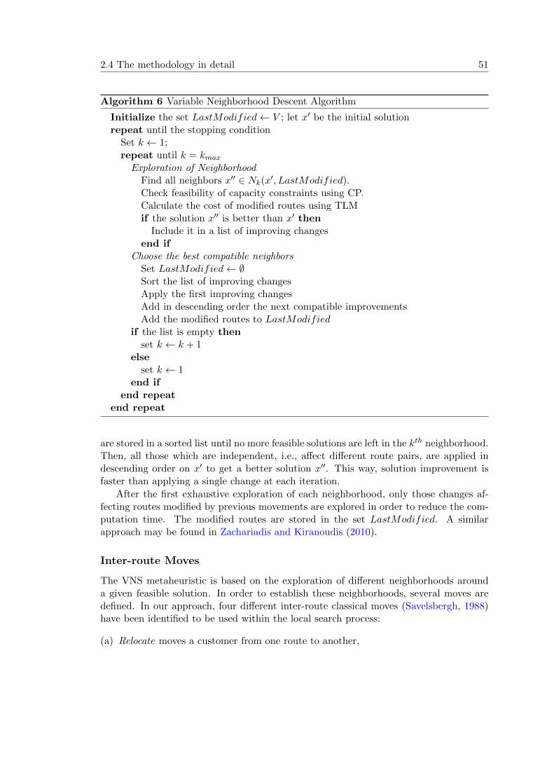
2.4 The methodology in detail 51
Algorithm 6 Variable Neighborhood Descent Algorithm
Initialize the set LastModified← V ; let x′ be the initial solutionrepeat until the stopping condition
Set k ← 1;repeat until k = kmax
Exploration of NeighborhoodFind all neighbors x′′ ∈ Nk(x
′, LastModified).Check feasibility of capacity constraints using CP.Calculate the cost of modified routes using TLMif the solution x′′ is better than x′ then
Include it in a list of improving changesend if
Choose the best compatible neighborsSet LastModified← ∅Sort the list of improving changesApply the first improving changesAdd in descending order the next compatible improvementsAdd the modified routes to LastModified
if the list is empty thenset k ← k + 1
elseset k ← 1
end ifend repeat
end repeat
are stored in a sorted list until no more feasible solutions are left in the kth neighborhood.Then, all those which are independent, i.e., affect different route pairs, are applied indescending order on x′ to get a better solution x′′. This way, solution improvement isfaster than applying a single change at each iteration.
After the first exhaustive exploration of each neighborhood, only those changes af-fecting routes modified by previous movements are explored in order to reduce the com-putation time. The modified routes are stored in the set LastModified. A similarapproach may be found in Zachariadis and Kiranoudis (2010).
Inter-route Moves
The VNS metaheuristic is based on the exploration of different neighborhoods arounda given feasible solution. In order to establish these neighborhoods, several moves aredefined. In our approach, four different inter-route classical moves (Savelsbergh, 1988)have been identified to be used within the local search process:
(a) Relocate moves a customer from one route to another,

52 Capacitated Vehicle Routing Problem
(b) Swapping exchanges two customers belonging to different routes,
(c) Chain is a specialization of 3-opt that swaps sections of two contiguous customersfrom different routes, and
(d) Ejection chain swaps the end portions of two different routes.
The use of our TLM ensures the partial optimality of most solutions from the routingperspective. The reason is that, since we are considering a relatively small number ofcustomers per route, the proposed approach can quickly find the optimal solution tomost TSP instances. In effect, the respective lower bounds (LB) and upper bounds(UB) converge rapidly, keeping their gap between 0 and 10−10, which guarantees thesolution optimality. In addition, it solves all routes in negligible times. Thus, it is anefficient alternative for intra-route optimization processes and avoids defining intra-routemoves.
2.5 Computational Results
The methodology described in this paper has been implemented in Java and linked to theopen-source CP software system ECLiPSe 6.0 (Apt & Wallace, 2007). All tests have beenperformed on a dedicated server with an Intel i5 processor at 2.66GHz and 16GB RAM.A total of 91 classical CVRP benchmark instances available at www.branchandcut.orghave been used to test the efficiency of the proposed approach when dealing with thissimple (in terms of constraints) but extensively tested scenario. In order to ensure fulfill-ment of the triangular inequality property, only those instances using Euclidean metricshave been selected. The selected problems also include 7 instances from (Christofides etal., 1979) (denoted in tables as C1-C5, C11, and C12) for further comparison with somerecent metaheuristics.
As the algorithm has been designed to be run in a parallel computing environment, atest has been done over the set A of benchmark problems to determine the most suitablenumber of simultaneous threads. This parameter is to be fixed mainly according tocomputer’s characteristics. In the particular server used in this work, up to 4 threadsmay be executed in parallel in order to keep a reasonable computational efficiency. In theperformed test, adopting a parallelized approach permits reducing the total computationtime significantly. In particular, for problems from the set A, the total computationtime is 41% lower, on average, than the total time spent using a sequential approach.For this reason, all results presented in this paper correspond to a Multi-Start VNDimplementation with 4 parallel processes, since this approach has demonstrated to keepa reasonable balance between the time spent on calculating one single solution and thetotal execution time.
Table 2.1 shows results obtained for some representative problems from the selectedbenchmark sets. Due to algorithm’s probabilistic behavior, the final solutions’ qualitydepends on the total number of threads. For this reason, 100 total tasks have beenconsidered for each problem, i.e., 100 pseudo-optimal solutions have been generated for

2.5 Computational Results 53
each benchmark instance. Table 2.1 summarizes information regarding the best solutionfound (OBS) for each problem, as well as the time required to reach this solution. Theseresults are compared to the best known solutions (BKS) so far. Most sources givethese values as integer numbers, obtained by rounding costs, except for the problemsfrom (Christofides et al., 1979) where real values are usually given. From the detailedinteger solutions, real costs have been calculated and reported. It should be remarkedthat the real cost of an integer optimal solution might not correspond to the optimalsolution considering real costs. For this reason, negative gaps appear on this table.Thus, it can be deduced that the Multi-Start VND is able to match, and in many casesimprove, the real value associated to the best known integer solutions. Concretely, thepresented approach has been able to improve 23 best known solutions, considering realcosts, out of the 91 tested instances. In addition, the gap is kept reasonably low for allconsidered instances, being the average gap 0.65 %. It remains lower, 0.17 %, for theproblems selected in Table 2.1, which include most of the largest instances.
Furthermore, it should be remarked that these results have been obtained in com-petitive times even for some large instances. As shown in Table 2.1, most solutions forsmall problems are obtained in less than a second, while larger instances require higheryet reasonable computational times. In most cases, higher times are closely related tohigher quality solutions, i.e., solutions with a negative gap.
Table 2.2 shows how these results are similar to other state-of-the-art metaheuristics.It provides a comparison between the proposed approach and some recent publications.The first three metaheuristics are: a hybrid algorithm of Simulated Annealing and TabuSearch (SA-TS) introduced in (Lin et al., 2009); a hybrid Electromagnetism-like heuristic(HEMA) proposed by Yurtkuran and Emel (2010); and a Particle Swarm algorithm(SR-2) described in (Jin Ai & Kachitvichyanukul, 2009). The next three metaheuristicscorrespond to our related work: a hybrid VNS (HVNS) presented in (Guimarans et al.,2011a); the randomized Clarke and Wright Savings (SR-GCWS) algorithm by Juan etal. (2010); and the Multi-Start VND presented in this chapter and in (Guimarans et al.,2011b).
Most publications only report results corresponding to the 14 instances from theworkbench presented by Christofides et al. (1979). For this reason, few results corre-sponding to other problem sets are reported for the first three metaheuristics in Table 2.2.Moreover, some of the instances from (Christofides et al., 1979) include an additionalconstraint on the maximum route length that is not handled in the proposed version ofthe algorithm. Therefore, results for these instances have been omitted in this table.
It may be observed that the proposed approach is comparable in terms of quality andcomputational efficiency to these recent metaheuristics. Times needed by our approachto reach a pseudo-optimal solution are in most cases lower than those required by meansof the other algorithms. It should be remarked that the proposed approach clearlyimproves the efficiency of the previous algorithms HVNS and SR-GCWS. Furthermore,the Multi-Start VND provides the lowest gap among all selected metaheuristics, onlybeated by the SR-GCWS approach. However, most of the higher gaps obtained withthe proposed approach correspond to some of the largest instances, whose results are

54 Capacitated Vehicle Routing Problem
Gap (%)Problem # nodes BKS OBS BKS-OBS # routes Time (s)A-n32-k5 31 787.81 787.08 -0.09 5 0.633A-n33-k5 32 662.76 662.11 -0.10 5 0.842A-n33-k6 32 742.83 742.69 -0.02 6 0.480A-n37-k5 36 672.59 673.59 0.15 5 1.948A-n37-k6 36 952.22 950.85 -0.14 6 1.631A-n38-k5 37 734.18 733.95 -0.03 5 2.546A-n45-k6 44 944.88 944.88 0.00 6 1.622A-n46-k7 45 918.46 918.13 -0.04 7 2.062A-n54-k7 53 1171.78 1171.78 0.00 7 4.007A-n55-k9 54 1074.46 1076.85 0.22 9 5.544A-n63-k9 62 1622.14 1622.14 0.00 9 8.073B-n31-k5 30 676.76 676.09 -0.10 5 0.657B-n34-k5 33 791.24 789.84 -0.18 5 0.497B-n35-k5 34 956.29 958.94 0.28 5 1.174B-n38-k6 37 809.45 809.45 0.00 6 1.211B-n39-k5 38 553.27 553.16 -0.02 5 1.577B-n43-k6 42 747.54 746.98 -0.07 6 1.520B-n45-k5 44 755.43 753.96 -0.19 5 1.011B-n50-k7 49 744.78 744.23 -0.07 7 1.721B-n50-k8 49 1316.20 1319.53 0.25 8 7.069B-n51-k7 50 1035.71 1037.54 0.18 7 597.915B-n57-k9 56 1603.63 1604.88 0.08 9 7.653B-n64-k9 63 869.32 868.31 -0.12 9 287.953E-n22-k4 21 375.28 375.28 0.00 4 0.337E-n23-k3 22 568.56 568.56 0.00 3 0.422E-n33-k4 32 838.72 837.67 -0.13 4 0.819E-n51-k5 (C1) 50 524.61 527.98 0.64 5 17.164E-n76-k10 (C2) 75 835.26 843.49 0.99 10 28.941E-n101-k8 (C3) 100 826.14 841.16 1.82 8 195.271F-n45-k4 44 724.57 727.75 0.44 4 4.459F-n135-k7 134 1170.65 1179.09 0.72 7 630.427G-n262-k25 261 5685.00 5722.00 0.65 25 1651.360M-n101-k10 (C12) 100 819.81 821.40 0.19 10 51.395M-n121-k7 (C11) 120 1042.11 1045.14 0.29 7 137.553M-n151-k12 (C4) 150 1028.42 1052.52 2.34 12 834.642M-n200-k17 (C5) 199 1291.45 1324.91 2.59 17 243.789P-n16-k8 15 451.95 451.95 0.00 8 0.019P-n19-k2 18 212.66 212.66 0.00 2 0.243P-n20-k2 19 217.42 217.42 0.00 2 0.148P-n21-k2 20 212.71 212.71 0.00 2 0.275P-n22-k2 21 217.85 217.85 0.00 2 0.277P-n23-k8 22 531.17 531.17 0.00 8 1.447P-n40-k5 39 461.73 461.73 0.00 5 6.189P-n45-k5 44 512.79 512.79 0.00 5 10.016P-n50-k7 49 559.86 560.15 0.05 7 5.155P-n51-k10 50 742.48 742.36 -0.02 10 5.156P-n55-k10 54 697.81 698.00 0.03 10 5.331P-n55-k8 54 592.17 581.17 -1.86 7 14.703P-n76-k5 75 635.04 633.32 -0.27 5 92.627P-n101-k4 100 692.28 693.54 0.18 4 839.622Average 0.17
Table 2.1: Results for 50 classical benchmark instances.
not reported for the SR-GCWS algorithm.

2.5 Computational Results 55
SA
-TS
HE
MA
SR
-2H
VN
SSR
-GC
WS
Mult
i-Sta
rtV
ND
Pro
ble
mB
KS
BS
t(s
)B
St
(s)
BS
t(s
)B
St
(s)
BS
t(s
)B
St
(s)
A-n
32-k
578
7.81
--
--
--
787.8
196.6
787.0
86.0
787.0
80.6
A-n
33-k
566
2.76
--
--
662.
7613
.0662.7
642.7
662.1
12.0
662.1
10.8
A-n
33-k
674
2.83
--
--
--
742.8
334.9
742.6
93.0
742.6
90.5
A-n
37-k
695
2.22
--
--
--
952.2
259.7
--
950.8
51.6
A-n
38-k
573
4.18
--
--
--
735.2
269.0
733.9
57.0
733.9
52.6
A-n
45-k
694
4.88
--
--
--
951.7
7141.7
944.8
831.0
944.8
81.6
A-n
46-k
791
8.46
--
--
918.
4623
.0919.2
0265.9
--
918.1
32.1
A-n
63-k
916
22.1
4-
--
--
-16
37.5
81254.3
1622.1
4145.0
1622.1
48.1
B-n
31-k
567
6.76
--
--
--
--
676.0
91.0
676.0
90.7
B-n
39-k
555
3.27
--
--
--
--
553.1
617.0
553.1
61.6
B-n
45-k
575
5.43
--
--
755.
4320
.0-
-754.2
220.0
753.9
61.0
B-n
50-k
774
4.78
--
--
--
--
744.2
32.0
744.2
31.7
E-n
33-k
483
8.72
--
--
--
--
837.6
77.0
837.6
70.8
E-n
51-k
5(C
1)52
4.61
524.
6138
.152
4.61
13.0
524.
6124
.0-
-524.6
132.0
527.9
817.2
E-n
76-k
10(C
2)83
5.26
835.
26118
.384
9.77
19.0
844.
4257
.0-
-835.2
621.7
843.4
928.9
E-n
101-
k8
(C3)
826.
1482
6.14
293
.384
4.72
41.0
829.
4010
1.0
830.5
340888.9
--
841.1
6195.3
M-n
101-
k10
(C12
)81
9.81
819.
5631
684
7.56
190.
081
9.56
88.0
841.3
712897.9
819.5
6338.0
821.4
051.4
M-n
121-
k7
(C11
)10
42.1
110
45.5
033
2.8
1042
.11
319.
010
52.3
493
.010
92.1
339383.9
1043.8
874.5
1045.1
4137.6
M-n
151-
k12
(C4)
1028
.42
1038
.71
701.
410
59.0
313
2.0
1048
.89
223.
010
35.8
076933.9
--
1052.5
2834.6
M-n
200-
k17
(C5)
1291
.45
1311
.70
1844
.313
02.3
320
1.0
1323
.89
413.
013
25.0
7195727.3
--
1324.9
1243.8
P-n
20-k
221
7.42
--
--
--
217.4
20.9
217.4
241.0
217.4
20.2
P-n
22-k
221
7.85
--
--
--
217.8
54.7
217.8
59.0
217.8
50.3
P-n
51-k
1074
2.48
--
--
--
742.4
8427.3
741.5
019.0
742.3
65.2
P-n
55-k
859
2.17
--
--
--
580.9
6247.7
--
581.1
714.7
P-n
76-k
563
5.04
--
--
--
633.3
210784.6
633.3
273.0
633.3
292.6
Ave
rage
gap
(%)
0.41
1.60
0.69
0.6
1-0
.05
0.2
3
Tab
le2.
2:C
omp
aris
onb
etw
een
the
pro
pos
edal
gori
thm
and
oth
erap
pro
ach
esfo
rso
me
class
ical
ben
chm
ark
inst
an
ces.

56 Capacitated Vehicle Routing Problem
As a final remark, it can be observed that the lowest gap (-1.86 %) corresponds tothe problem P-n55-k8, where a solution considering only 7 vehicles (# routes) has beenobtained. Although the best known solution for this problem uses 8 vehicles, feasiblesolutions with 7 vehicles and lower costs may be reached, as the one obtained with thisapproach. However, if only 7 vehicles are considered, the Multi-Start VND has finishedslightly over the value 580.96 (576 considering integer costs), published for this problemin (Guimarans et al., 2011a), (Alba & Dorronsoro, 2008), and (Altinel & Oncan, 2005).
2.6 Conclusions
The described hybrid algorithm embeds CP and TLM within the VND metaheuris-tics framework by decomposing the CVRP into two subproblems concerning customers’allocation and routing optimization separately. This approach allows reducing the com-putation time during local search processes, since problems to be solved are far lesscomplex than the original CVRP.
A fast and efficient algorithm such as the randomized CWS algorithm is used tofeed the multi-start scheme by generating good initial solutions. Thus, the proposed op-timization approach implements a flexible, efficient and robust optimization algorithmable to deal with some realistic problems, which means both the ability to tackle largeinstances and to represent real operational constraints. The characteristics of the re-sulting algorithm can be explained in the following way: flexibility involves the qualityof the algorithm to be adapted to real problems; efficiency is related to the easiness ofthe algorithm to obtain optimal or quasi-optimal solutions in reasonable computationtimes; and robustness is related to the fact that the algorithm performs well even whenno extensive fine-tuning processes are carried out on its parameters.
Regarding flexibility, this approach benefits from the CP capabilities to model differ-ent operational constraints. This constraints are present in most of the real applicationcases and, in general, affect to the allocation decisions. CP, which is not restricted bymodeling limitations such as constraint linearity, facilitates the representation of allo-cation constraints without requiring any specific action on the solving method. Hence,the hybrid scheme can be easily adapted to different CVRP variants by simply addingthe allocation constraints which properly model the feasible solutions of the problem.Since the VND optimization scheme is able to reach feasible solutions starting from non-feasible initial solutions, e.g., not fulfilling the maximum number of vehicles (Guimaranset al., 2010), the RCWS algorithm does not need to be modified in order to includeoperational constraints other than capacities. However, other capacity-like constraints,such as total driving time of each route, can be translated to a capacity constraint inorder to obtain feasible solutions by means of the RCWS algorithm. Additional opera-tional constraints may be added to the CP model, which will ensure solutions’ feasibilityalong the local search process. Thus, this hybrid approach will be able to tackle complexinstances related to real application cases by adding little modifications into the problemmodeling, but neither into the optimization scheme nor algorithms.
The efficiency of the proposed algorithm is supported by the results presented in the

2.6 Conclusions 57
previous section. As discussed, the presented approach is able to match the best knownsolutions for benchmark problems of different sizes in reasonable computation times.The provided comparison proves that its efficiency is similar to other state-of-the-artmetaheuristics, both in terms of time and solutions’ quality.
The robustness of the algorithm is a consequence of the light requirements for finetuning. Our TLM metaheuristic does not require any specific adjustment since all theconvergence parameters are self-tuned. The CP-based subproblem depends just on thequality of the defined constraint model to properly describe the feasible solutions. TheRCWS does not require any adaptation either. Only the VND movements could requiredifferent priorities depending on the problem being solved in order to get a better solutionquality.
Our proposed Tailored Lagrangian Metaheuristic has been used to calculate routingcost for each vehicle separately. It solves all routes in negligible times and is an efficientalternative for intra-route optimization processes and avoids defining intra-route moves.Moreover, it ensures the partial optimality of most solutions from the routing perspective.The reason is that, since we are considering a relatively small number of customersper route, the proposed approach can quickly find the optimal solution to most TSPinstances.


Chapter 3
Workload-Balanced andLoyalty-EnhancedHome Health Care
This chapter describes a practical application concerning the Home Health Care (HHC)service in the municipality of Ferrara, a mid-sized city in the North of Italy. The problemhas been solved using a hybrid methodology based on Large Neighborhood Search (LNS)combining Constraint Programming (CP) and our Tailored Lagrangian Metaheuristic(TLM) proposed in Section 1.6.
Although sometimes it is necessary, no one likes to stay in a hospital, and patientswho need to stay in bed but do not require constant medical surveillance prefer theirown bed at home. At the same time, a patient in a hospital has a high cost for thecommunity, that is not acceptable if the patient needs service only a few minutes a day.For these reasons, the Health Services providers in Europe and North America havetried to avoid the hospitalization of patients whenever possible. A patient that has tostay in a hospital has a high cost for the community, and saving money (and resources)means that those resources can be spent for providing a better service to other patients.Hence the current trend is to send nurses to visit patients at their home where patientsperceive a higher quality of life, with their dear ones, and feel their illness more similarto a “normal” life situation. This reduces depression risk for the patient, and improvesrehabilitation rate. Indeed, high quality Home Health Care following hospital dismissalhas proved essential in reducing hospital readmissions, if able to cope with preventablecomplications.
The challenge is to deliver the service in a cost effective manner without a detri-ment of the service quality. These social and health management issues have interestingimplications from the mathematical viewpoint, introducing a challenging combinatorialoptimization problem. The problem consists on assigning patients’ services to travelingnurses and defining the nurse itineraries so that the following optimization aspects areconsidered: the nurse workloads (including service as well as travel time) are balanced,patients are preferentially served by a single nurse or just a few ones, and the overall
59

60 Workload-Balanced and Loyalty-Enhanced Home Health Care
travel time is minimized. These objectives are somehow conflicting and a reasonabletrade off must be found. The complexity of the problem calls for suitable optimization-based algorithmic supports to decisions, in particular in the perspective of an increasingdiffusion of the service. This HHC problem is currently solved by hand, starting froma partitioning of patients based on predefined zones. We describe a CP model thatsolves the HHC problem, and show significant improvements with respect to the currentmanual solution.
Arguments in favor of Home Health Care and how to reduce health related risks whenclinical service is provided at home can be found also in (Giuliani et al., 2005) and (Mileoet al., 2011). When a patient requires service only for a limited time per day, or even perweek, then it is a viable and convenient solution to send nurses to provide the serviceat the patient’s home. Managing such a service gives rise to a family of challengingoptimization problems referred to as Home Health Care routing and scheduling (see(Bertels & Fahle, 2006) and (Steeg & Schroder, 2008)).
The work presented in this chapter has a previous version presented in (Cattafi etal., 2012), it was in ECLiPSe (Schimpf & Shen, 2012), which is a logic programmingsystem, so we defined a declarative semantics for the traveltime constraint. The currentversion is presented in (Cattafi et al., 2015), and it extends in several directions:
• a new implementation in the language Comet, which has more global constraints,that have powerful constraint propagation, and allowed us to improve the efficiencyof the application;
• new search algorithms, based on Large Neighborhood Search, that let us get tobetter solutions in shorter time;
• a wider experimentation;
• the use of a new objective function.
3.1 Problem Definition: the Home Health Care service inFerrara
At present, the HHC service in the city of Ferrara, Italy, is directly administrated bythe local agency of the National Health Service (NHS), namely AUSL 109. All patientswho are not self sufficient and in need of medical treatment are eligible for HHC, i.e.,any person who is infirm, chronically ill, or disabled. A demand for assistance mustbe issued by the family doctor to AUSL 109, specifying the list of required medicaltreatments. If the demand is accepted, the patient is enrolled in the service, and therequired treatments are entered into the request data base. Each request is characterizedby a patient identifier (name and address), a medical treatment, and the specific day ofthe week when the treatment must be delivered (each patient can have more than onerequest per week).
Service is provided by a set of qualified nurses, all registered nurses with additionaltraining, employed by the local NHS agency. Every day, each nurse who is on duty

3.1 Problem Definition 61
starts the shift at the city hospital, visits the patients in the list delivering the requiredtreatments and traveling by car from one patient’s home to the next; finally the nursereturns to the hospital.
A total of 15 nurses is involved and they are organized as follows. On working days,i.e., from Monday to Friday, 12 nurses are on duty. 9 of them operate in the morningwhile 3 in the afternoon. During weekends, 4 nurses work on Saturday and 1 on Sundayor during holidays.
Working rules. A duty should last up to 7 hours and 12 minutes on a working day, andabout 6 hours on Saturdays and holidays. This limit is not strictly enforced, providedthat the threshold of 36 hours per week is not exceeded over a planning horizon of 4weeks.
Each nurse works 5 days a week (on working days only) each alternate week andworks 6 days the other week; the sixth day is usually a Saturday, but it can be a Sundayonce every 14 weeks.
Lunch breaks are not present because shifts are either morning or afternoon. Allnurses have same starting and ending times, and must start and end shifts at the hospital.Nurse unavailabilities are considered unexpected events, and one additional nurse isalways available for such emergency.
Service Time
First visit 1 hourEnema 30 minGeneral check 15 minTracheotomy check and tube change 15 minCentral venous catheter 30 minElectrocardiogram 30 minEmogasanalysis 15 minMouth cleaning 5 min
Table 3.1: Excerpt of the services with average service time
Services consist of treatments and medications, and since their delivery time hasalmost no impact on the patient daily routine (patients stay in bed almost all day),there are no time windows. A treatment lasts from 5 to 60 minutes, depending on itsspecific characteristics (see Table 3.1 for an excerpt), but a patient in a day may needseveral treatments, that are carried out as a whole by a single nurse and handled as asingle request. Therefore, requests duration is quite heterogeneous over the whole set ofrequests, as can be seen on Figure 3.2.
Ferrara has about 150,000 inhabitants, and the area administered by AUSL 109 israther large and its population ageing. Most of the elderly patients live in the coun-tryside, so there is a significant geographical dispersion of the requests. Therefore, the

62 Workload-Balanced and Loyalty-Enhanced Home Health Care
�� �� �� �� �� �� �� �� � �� ��� ��� ��� ��� ��� ��� �����
�
�
�
�
�
�
�
�
���������������������������������������������
����������������� !��"
��
������
Figure 3.2: Histogram of the frequency of service durations in a typical day
service is characterized by a high variance of duration and a significant geographicaldispersion of the requests.
As a sample of the set of requests, we consider the month of February 2010, with3323 requests subdivided among 458 patients. Several patients are located either in townor in its suburbs, though quite a few live in the neighboring towns of Masi Torello andVoghiera, that are approximately 20km away.
At present, the digitization of data is limited to the patient data base, containingthe address and the prescribed services for each patient. The duty definition and themanagement of nurse agendas is handled manually and supervised by the chief nurse,with frequent adjustments done by cell phone. As a record of their duty, nurses fill formson paper which they return to the chief nurse at the end of their daily shift.
The problem data
Optimizing the HHC scheduling is essential to make the service cost-effective and to avoidthe so called burn out phenomenon, i.e., nurses who get tired and act in an unfriendlymanner to patients or even leave the job. At the same time, also the patient point ofview should be accounted for. Specifically, a patient would like to receive cares alwaysby the same nurse or by a few ones, if possible, since receiving clinical care involvesphysical and emotional contacts that one is not like to easily share with anyone. Thisintroduces the concept of loyalty (i.e., the number of different nurses per patient) as ameasure of the service quality as it is perceived from the patient viewpoint.
We start by examining the current solution approach, as it is manually carried outby the people in AUSL 109, and analysing its critical aspects. Nurses organize theirduties themselves, solving the problem by hand according to the following procedure.
To simplify the assignment of patients to nurses, the territory pertaining AUSL109 is statically partitioned into 9 zones (see Figure 3.3), considering factors like the

3.1 Problem Definition 63
Figure 3.3: The 9 zones in which the city is divided, with shown the location of thepatients
distribution of the population, its age and historical data. As we can see from Figure 3.3,some zones are in the city center, they are very small, but they have a large numberof patients that require service. Other zones are in peripheral areas, and they are lessdensely populated. A nurse assigned to a central zone will probably have many patientsto serve, while a nurse assigned to a peripheral zone will likely spend a significant amountof time traveling.
Each nurse receives in charge the services of all the patients belonging to one area.Then the nurse tries to fit the requests for the whole week into the working shifts, whilecomplying with the maximum weekly workload allowed, since no overduty is permitted.The assignment of requests to daily shifts follows a sort of greedy criterion: nurses, byhand, insert as many requests as possible into the shifts. There are no given rules onwhich patients to select first: each nurse could use a different order, in principle. Suchdecisions are not driven by any optimization criteria, and the routing is not necessarilyoptimal.
If a nurse can not fulfill all the requests, some requests are forwarded to the chiefnurse, who is in charge of the service coordination, and reassigns them to other colleagues.In such a case, a patient may be treated by different nurses at different days of the week,which goes to the detriment of the service quality. The three nurses working in theafternoon are in charge of the remaining requests, that are still assigned to the nurseson the basis of a similar geographical partition of the territory, each nurse dealing withthe patients of three zones. Therefore, patients are supposed to be visited along themorning, but maybe they are visited in the afternoon. Currently, patients do not knowthe schedule.
Due to this greedy procedure, the nurse weekly schedules have very different work-loads, and balancing this over the months leads to a detriment in loyalty. Nurses com-plain about such disparities, and have difficulties adapting their schedule to new patients,
64 Workload-Balanced and Loyalty-Enhanced Home Health Care
new treatments, or to any other change. Moreover, if the workload balance could beimproved by optimizing the routing component, nurses could be available at the hospi-tal for other tasks. In addition, an improved routing plan would impact on the directexpenses related to fuel and car usage, which contribute to the overall cost.
The decisions to be taken are:
• partitioning the requests to a set of duties,
• for each duty determining the sequence of services to be carried out optimizing thetraveling times by solving a Traveling Salesman Problem (TSP), and
• assigning each duty to a nurse to build the nurse weekly schedule.
Scheduling such a service poses several challenges, related to the criteria which char-acterize high quality solutions. A good solution should achieve at the same time:
• from the point of view of the NHS, the minimization of the travel time over theservice time, since during travel a nurse is on duty but is not delivering any service;
• from the point of view of the nurses, a fair distribution of the workload, which cannot be guaranteed by simply equally subdividing patients, due to heterogeneousrequests;
• from the point of view of the patients, a high degree of loyalty, i.e., the number ofdifferent nurses who are in charge of a single patient should be minimal.
The problem we are facing contains several subproblems, namely assigning eachrequest to one available nurse, scheduling optimally the services in each nurse’s duty,and finding the optimal route for each nurse in order to avoid long useless trips. We willdescribe in the following the main components of the CP-based hybrid solution approachthat has been developed to tackle such a difficult problem.
3.2 Literature Review
The efficient delivery of Home Health Care service is increasingly attracting the attentionof the Artificial Intelligence and the Operations Research communities. Most of the con-tributions focus on the application aspects and often, beside the optimization approach,they describe the complete information system managing the service. Therefore thespecific application aspects strongly characterize the optimization problems presented ineach paper and the proposed solution methods. This is the reason why, in practice, eachpaper addresses a different problem and a thorough comparison can be hardly done.
The great majority of the contributions consider a service where patients/users spec-ify a (more or less narrow) time window when they are available to receive the service.This feature is typical of the systems where the service is managed in conjunction witha Home Care. In Home Care services the presence of time windows is crucial since usersare supposed to be independent and to move from their home. This is not the case of
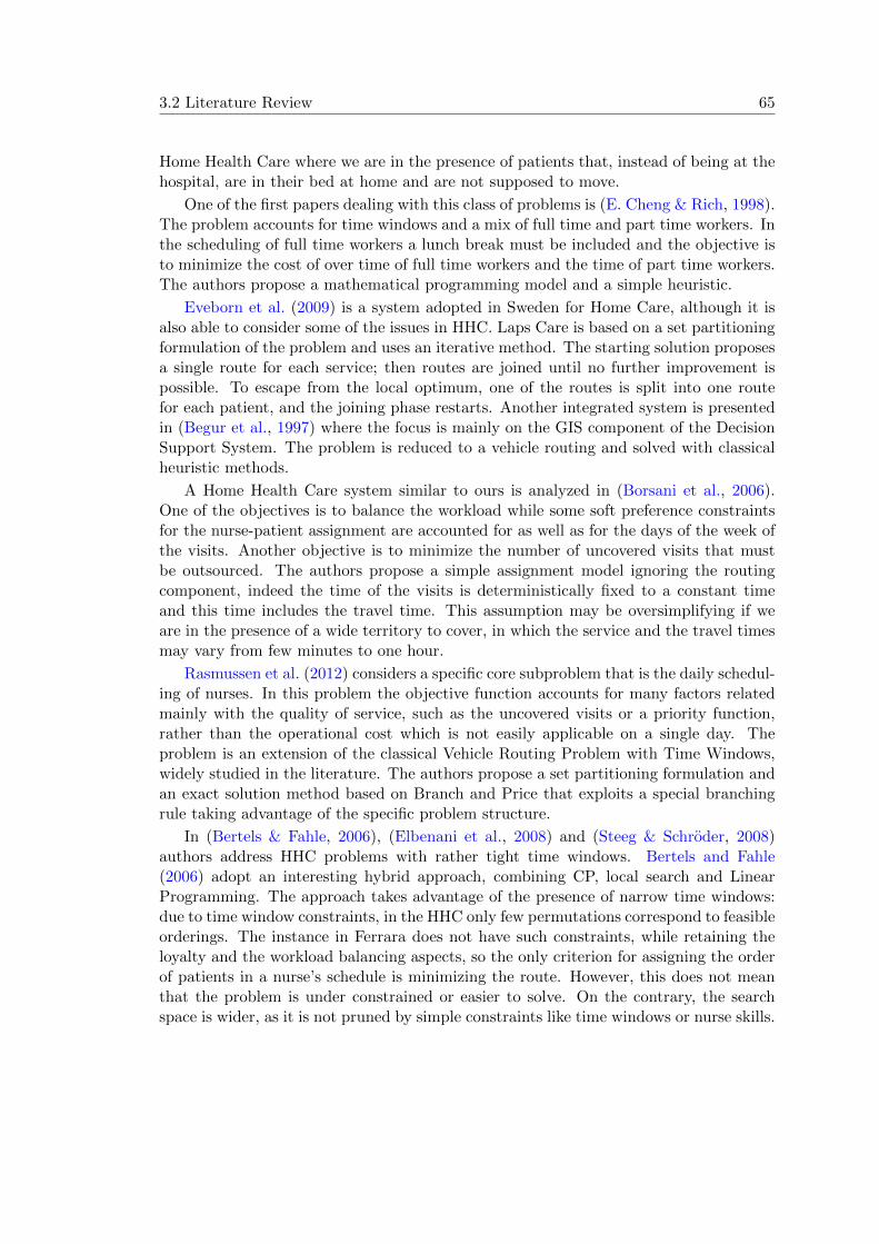
3.2 Literature Review 65
Home Health Care where we are in the presence of patients that, instead of being at thehospital, are in their bed at home and are not supposed to move.
One of the first papers dealing with this class of problems is (E. Cheng & Rich, 1998).The problem accounts for time windows and a mix of full time and part time workers. Inthe scheduling of full time workers a lunch break must be included and the objective isto minimize the cost of over time of full time workers and the time of part time workers.The authors propose a mathematical programming model and a simple heuristic.
Eveborn et al. (2009) is a system adopted in Sweden for Home Care, although it isalso able to consider some of the issues in HHC. Laps Care is based on a set partitioningformulation of the problem and uses an iterative method. The starting solution proposesa single route for each service; then routes are joined until no further improvement ispossible. To escape from the local optimum, one of the routes is split into one routefor each patient, and the joining phase restarts. Another integrated system is presentedin (Begur et al., 1997) where the focus is mainly on the GIS component of the DecisionSupport System. The problem is reduced to a vehicle routing and solved with classicalheuristic methods.
A Home Health Care system similar to ours is analyzed in (Borsani et al., 2006).One of the objectives is to balance the workload while some soft preference constraintsfor the nurse-patient assignment are accounted for as well as for the days of the week ofthe visits. Another objective is to minimize the number of uncovered visits that mustbe outsourced. The authors propose a simple assignment model ignoring the routingcomponent, indeed the time of the visits is deterministically fixed to a constant timeand this time includes the travel time. This assumption may be oversimplifying if weare in the presence of a wide territory to cover, in which the service and the travel timesmay vary from few minutes to one hour.
Rasmussen et al. (2012) considers a specific core subproblem that is the daily schedul-ing of nurses. In this problem the objective function accounts for many factors relatedmainly with the quality of service, such as the uncovered visits or a priority function,rather than the operational cost which is not easily applicable on a single day. Theproblem is an extension of the classical Vehicle Routing Problem with Time Windows,widely studied in the literature. The authors propose a set partitioning formulation andan exact solution method based on Branch and Price that exploits a special branchingrule taking advantage of the specific problem structure.
In (Bertels & Fahle, 2006), (Elbenani et al., 2008) and (Steeg & Schroder, 2008)authors address HHC problems with rather tight time windows. Bertels and Fahle(2006) adopt an interesting hybrid approach, combining CP, local search and LinearProgramming. The approach takes advantage of the presence of narrow time windows:due to time window constraints, in the HHC only few permutations correspond to feasibleorderings. The instance in Ferrara does not have such constraints, while retaining theloyalty and the workload balancing aspects, so the only criterion for assigning the orderof patients in a nurse’s schedule is minimizing the route. However, this does not meanthat the problem is under constrained or easier to solve. On the contrary, the searchspace is wider, as it is not pruned by simple constraints like time windows or nurse skills.
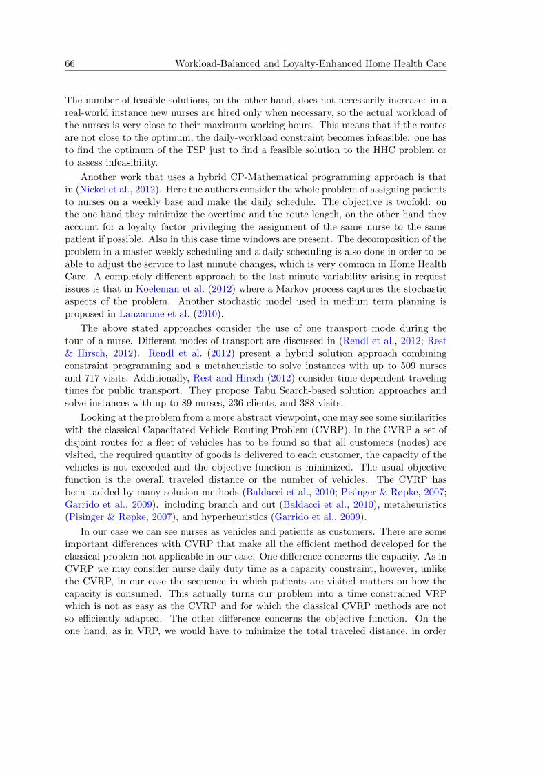
66 Workload-Balanced and Loyalty-Enhanced Home Health Care
The number of feasible solutions, on the other hand, does not necessarily increase: in areal-world instance new nurses are hired only when necessary, so the actual workload ofthe nurses is very close to their maximum working hours. This means that if the routesare not close to the optimum, the daily-workload constraint becomes infeasible: one hasto find the optimum of the TSP just to find a feasible solution to the HHC problem orto assess infeasibility.
Another work that uses a hybrid CP-Mathematical programming approach is thatin (Nickel et al., 2012). Here the authors consider the whole problem of assigning patientsto nurses on a weekly base and make the daily schedule. The objective is twofold: onthe one hand they minimize the overtime and the route length, on the other hand theyaccount for a loyalty factor privileging the assignment of the same nurse to the samepatient if possible. Also in this case time windows are present. The decomposition of theproblem in a master weekly scheduling and a daily scheduling is also done in order to beable to adjust the service to last minute changes, which is very common in Home HealthCare. A completely different approach to the last minute variability arising in requestissues is that in Koeleman et al. (2012) where a Markov process captures the stochasticaspects of the problem. Another stochastic model used in medium term planning isproposed in Lanzarone et al. (2010).
The above stated approaches consider the use of one transport mode during thetour of a nurse. Different modes of transport are discussed in (Rendl et al., 2012; Rest& Hirsch, 2012). Rendl et al. (2012) present a hybrid solution approach combiningconstraint programming and a metaheuristic to solve instances with up to 509 nursesand 717 visits. Additionally, Rest and Hirsch (2012) consider time-dependent travelingtimes for public transport. They propose Tabu Search-based solution approaches andsolve instances with up to 89 nurses, 236 clients, and 388 visits.
Looking at the problem from a more abstract viewpoint, one may see some similaritieswith the classical Capacitated Vehicle Routing Problem (CVRP). In the CVRP a set ofdisjoint routes for a fleet of vehicles has to be found so that all customers (nodes) arevisited, the required quantity of goods is delivered to each customer, the capacity of thevehicles is not exceeded and the objective function is minimized. The usual objectivefunction is the overall traveled distance or the number of vehicles. The CVRP hasbeen tackled by many solution methods (Baldacci et al., 2010; Pisinger & Røpke, 2007;Garrido et al., 2009). including branch and cut (Baldacci et al., 2010), metaheuristics(Pisinger & Røpke, 2007), and hyperheuristics (Garrido et al., 2009).
In our case we can see nurses as vehicles and patients as customers. There are someimportant differences with CVRP that make all the efficient method developed for theclassical problem not applicable in our case. One difference concerns the capacity. As inCVRP we may consider nurse daily duty time as a capacity constraint, however, unlikethe CVRP, in our case the sequence in which patients are visited matters on how thecapacity is consumed. This actually turns our problem into a time constrained VRPwhich is not as easy as the CVRP and for which the classical CVRP methods are notso efficiently adapted. The other difference concerns the objective function. On theone hand, as in VRP, we would have to minimize the total traveled distance, in order

3.3 The Methodology in detail 67
to make the service as efficient as possible, on the other hand we have to balance theworkload among nurses. Thus this component of the objective function is a kind ofbottleneck (min-max), that is difficult to address with OR methods. Finally, the loyaltyis the component of the objective function that makes our problem very peculiar. Thetwo criteria are often in contrast: any solution assigning to a single nurse all the servicesof the same patient would minimize the loyalty, but this would go to the detriment ofworkload balancing.
3.3 The Methodology in detail
A hybrid methodology based on Large Neighborhood Search is presented in this section,it combines Constraint Programming (CP) and the Tailored Lagrangian Metaheuristic(TLM) proposed in Section 1.6. This section is structured as follows: the input datais described, the CP model is presented, then the objective function is discussed, it isexplained how the routing is addressed and finally the search strategy is presented.
LNS is becoming more and more popular to solve routing problems, an introductioncan be found on page 17 and in (Shaw, 1998; Pesant et al., 1997). The idea is alocal search that adopts a large neighborhood which makes less likely to fall in a localminimum. Exploring the neighborhood becomes a search problem itself, and it is donewith CP. In this way, it is possible to take into account easily many side constraints.
The popularity of hybridization of CP and Local Search (Monfroy et al., 2004; Wal-lace, 2006) is witnessed by the existence of solvers tailored for this approach (Van Hen-tenryck & Michel, 2009), and the application to routing problems (Rousseau et al., 2002;Kilby et al., 2000). Various works deal with solving the TSP or its variant with CP orhybrid algorithms (Caseau & Laburthe, 1997; Pesant et al., 1998; Focacci et al., 2002).Rousseau et al. (2002) propose a large neighborhood search in which CP explores aneighborhood with three operators. These operators are combined in variable neigh-borhood descent and a two phase process. Kilby et al. (2000) consider vehicle routingproblems with side constraints, and compare classical OR approaches with CP models.OR approaches tend to use cost-oriented heuristics, that make them suitable for prob-lems with few side constraints, but fail to find an initial solution when the number ofside constraints grows. On the other hand, CP approaches are better when the sideconstraints are more tight but usually provide worse solutions when the side constraintsare not prevalent.
We believe that using CP to tackle this problem is a wise choice, because of theimportance of the feasibility issues represented by the time constraints, of the manyaspects which can benefit of CP’s flexibility (such as the need to easily add and relaxconstraints to follow change in the requirements) and because CP provides an effectiveframework for the integration of components based on different approaches. In thissection we will explain the CP model and we will deal with some of these issues.

68 Workload-Balanced and Loyalty-Enhanced Home Health Care
Input Description
The input data consists of:
• a set Sserv of services, of size Ns; for each service s we know the patient pats, theday days and the duration durs;
• a matrix of distances D where the element di,j is the travel time from patient i topatient j;
• the number of nurses Nn;
• the set of nurses Snurse (i.e., Nn = |Snurse| or Snurse = {1, . . . , Nn});
• the number of days Nd considered in the scheduling;
• the maximum time that a nurse can spend working each day; MaxDayWL is theamount of minutes available per day for each nurse (including service time andtravel time); it currently corresponds to 7 hours and 12 minutes (432 minutes);
• the maximum time that a nurse can spend working in a week; MaxWeekWL is thenumber of minutes available per week for each nurse. It currently corresponds to36 hours.
The CP Model
A constraint model is defined by a set of decision variables (unknowns), each rangingon a given domain, and a set of constraints, that each assignment must satisfy. Often,there is also an objective function, that should be minimized or maximized. A solutionis an assignment of values taken from the domains to the corresponding variables suchthat all constraints are satisfied, and that minimizes (resp. maximizes) the objectivefunction.
Usually an efficient model makes use of global constraints, i.e., constraints that involvemany (possibly, all) variables in the model. Often, global constraints propagate moreefficiently than small constraints that involve only two or three variables. We show amodel that includes a number of global constraints.
Variables:
The main decision is assigning nurses to services. To each service s we associate adecision variable Nurses with domain Snurse.
Other variables have functional dependency to the Nurses variables. For each nursen and day d, we have a decision variable DayWLn,d with domain {0..MaxDayWL}. Thisis the number of minutes worked by nurse n on day d.
Other variables represent service time and traveling time: T svcn,d and T trvn,d are, respec-tively, the service time and the travel time of nurse n in day d; they also range from 0to the maximum day workload MaxDayWL.

3.3 The Methodology in detail 69
We also have variables containing the weekly totals: each nurse n has a weekly traveltime WT trvn , a weekly service time WT svcn , and a weekly workload WLn, that is the sumof the travel and service time; their domain is {0..MaxWeekWL}.
Another decision to be taken is the order in which a nurse visits the assigned patients.This problem will be dealt with in “Addressing the Routing” on page 75.
Constraints:
The workload of a nurse n in a day d is the sum of the total service time and the traveltime
DayWLn,d = T svcn,d + T trvn,d , (3.1)
while the (whole week) workload WLn is simply the sum of the day workloads:
WLn =
Nd∑d=1
DayWLn,d (∀n ∈ Snurse).
The service time is the sum of the duration of the services provided by nurse n inday d. In order to compute the service time of each nurse in each day (and to enforce atthe same time that the total service time does not exceed the maximum day workloadMaxDayWL), there can be different constraint models. An intuitive model could be todefine a set of Boolean decision variablesXn,s (variables taking values true or false) sayingif nurse n takes service s, and add corresponding sum constraints. A more promisingmodel can be obtained noticing similarities with classic problems such as bin packingand (multi)-knapsack problems (Korf, 2003; Fukunaga & Korf, 2007).
In a multi-knapsack problem, a set of Nitems items with size sizei have to be placedin a set Nk of containers without exceeding their capacities.
The global constraint multiknapsack (also called binpacking) (Shaw, 2004) is suitedto solve such problems. In CP a multiknapsack problem can be simply defined with theconstraint
multiknapsack(a, size, load)
where
• a ≡ {ai} is a set of decision variables ai with domain
ai :: 1..Nk (∀i ∈ 1..Nitems),
with the intended meaning that ai = j if only if item i is assigned to knapsack j;
• size ≡ {sizei} is the array containing the size of each item
• load ≡ {loadj} is a set of constrained variables that represent the actual load ofeach knapsack, i.e., the sum of the sizes of the items assigned to that knapsack.In order to solve a multi-knapsack problem, the loadj domains are constrained totake values up to the capacity of the knapsacks:
loadj ≤ capacityj (∀j ∈ 1..Nknapsacks).

70 Workload-Balanced and Loyalty-Enhanced Home Health Care
By using the techniques currently embedded in the multiknapsack constraint, Shaw(2004) obtains a speedup of several orders of magnitude with respect to the intuitivemodel, so we decided to take this second approach.
In the HHC problem, we can consider
• each service s as an item of size durs which has to be placed in one of thebins/knapsacks;
• to each pair (nurse, day) we associate a knapsack of capacity MaxDayWL;
• the actual load of knapsack (nurse, day) is the service time T svcnurse,day of nursenurse in day day.
We can thus bind the Nurse decision variables with the whole T svc vector. We imposethe constraint
multiknapsack (Nurse, dur, T svc) ,
which enforces that (∀n ∈ Snurse, ∀d ∈ {1..Nd}):
T svcn,d =∑
s∈Sservd=days
[Nurses = n]× durs
where the square brackets are the Iverson brackets (Knuth, 1992)1.
The travel time T trvn,d of nurse n in day d is computed by a specific constrainttraveltime, explained in detail in “Addressing the Routing” on page 75.
The Objective Function
Ideally, in the HHC problem in Ferrara, one should find a solution that achieves theobjectives described in the introduction. As it is often the case in real world applications,the objectives are stated by the users in a blurred, informal way, not clear enough toconvert them into a unique objective function, and all functions one can think of aredebatable. The main objectives, as stated by the user, are to (i) avoid that a patient isvisited by too many different nurses (loyalty) and (ii) balance the weekly workloads ofthe nurses (but they also have to keep reasonable conditions for all nurses and for theNHS).
We first address the two issues separately, then we combine them.
Loyalty One way to obtain maximum loyalty is to minimize the number of nurses thatvisit each patient. For each patient p ∈ Spatient we link the array of decision variablesNursep with the number of different values in it.2 The alldifferent (Regin, 1994; van Ho-eve, 2001) global constraint enforces that all the variables in an array are given different
1let P be a statement, [P ] evaluates to 1 if P is true and to 0 otherwise.2To simplify the notation, we indicate with Nursep the subset of the Nurse array corresponding to
patient p.

3.3 The Methodology in detail 71
values. The global constraint NV alue (Bessiere et al., 2006; Hebrard et al., 2011; vanHoeve, 2004) can be thought of as a soft version of alldifferent, and it counts the numberof different values in a vector of variables. Various efficient propagation algorithms havebeen proposed for the NValue constraint; using the global constraint NValue is usuallyconsidered more efficient than using a set of smaller constraints (Bessiere et al., 2010).By counting the different values in the set of decision variables associated to a certainpatient p, we obtain the number PNp of different nurses who take care of that patient:
NValue(Nursep, PNp) (∀p ∈ Spatient)
and we can compute the overall loyalty penalty LP summing up the single contributions:
LP =∑
p∈Spatient
PNp. (3.2)
Balancing workloads There are various ways to achieve balanced workloads, see(Simonis, 2007). A widely used method is the minimization of the maximum workload,so a first proposal is to minimize:
BalanceWL′ = MaxWL = maxn∈Snurse
(WLn). (3.3)
There are known pitfalls in adopting the minimization of the maximum (see, e.g.,(Monette et al., 2007)). One simple observation is that two solutions are consideredequivalent if they have the same value for the highest workload, regardless of the workingconditions of all other nurses.
Consider for instance the following example, also depicted in Figure 3.4:
Example 1 Suppose that there is a patient X that lives rather far from the hospital, andalso requires a long service time (Figure 3.4); suppose that, in order to visit and servicehim, a nurse takes a time exactly equal to the maximum day workload MaxDayWL. Theother patients, instead, live close to the hospital and have shorter service times. In sucha case, one nurse will serve only patient X, while the other patients will be subdividedamong the other nurses.
In this example, the minimization of the maximum workload provides the same valuefor all the possible assignments: the maximum workload is fixed to the maximum dayworkload, and corresponds to the nurse visiting patient X.
More recent proposals to obtain balanced solutions are the spread (Pesant & Regin,2005) and deviation (Schaus et al., 2007) constraints. These constraints link a set ofdecision variables with their variance or with the mean absolute deviation. In this way,it is both simple to define objective functions that minimize the variance (resp. meanabsolute deviation), and efficient, thanks to the powerful global constraint propagators.In our application, we decided to experiment with the deviation constraint, thus min-imizing the L1 norm although, as noticed in (Schaus et al., 2009), “These criteria are
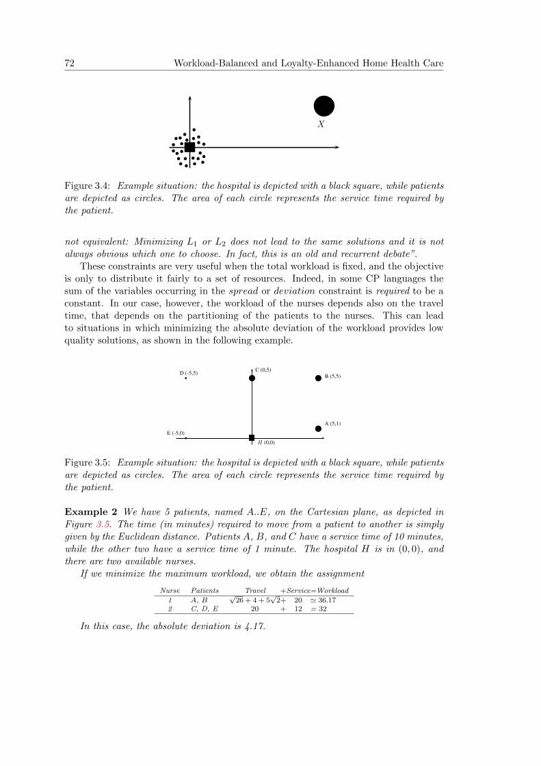
72 Workload-Balanced and Loyalty-Enhanced Home Health Care
b
bb
b bb
b
bb
bb b
b b
bbb
bb
bb
b
bb
X
Figure 3.4: Example situation: the hospital is depicted with a black square, while patientsare depicted as circles. The area of each circle represents the service time required bythe patient.
not equivalent: Minimizing L1 or L2 does not lead to the same solutions and it is notalways obvious which one to choose. In fact, this is an old and recurrent debate”.
These constraints are very useful when the total workload is fixed, and the objectiveis only to distribute it fairly to a set of resources. Indeed, in some CP languages thesum of the variables occurring in the spread or deviation constraint is required to be aconstant. In our case, however, the workload of the nurses depends also on the traveltime, that depends on the partitioning of the patients to the nurses. This can leadto situations in which minimizing the absolute deviation of the workload provides lowquality solutions, as shown in the following example.
b
bb
b
b
A (5,1)
B (5,5)C (0,5)D (-5,5)
E (-5,0)
H (0,0)
Figure 3.5: Example situation: the hospital is depicted with a black square, while patientsare depicted as circles. The area of each circle represents the service time required bythe patient.
Example 2 We have 5 patients, named A..E, on the Cartesian plane, as depicted inFigure 3.5. The time (in minutes) required to move from a patient to another is simplygiven by the Euclidean distance. Patients A, B, and C have a service time of 10 minutes,while the other two have a service time of 1 minute. The hospital H is in (0, 0), andthere are two available nurses.
If we minimize the maximum workload, we obtain the assignment
Nurse Patients Travel +Service=Workload
1 A, B√
26 + 4 + 5√
2+ 20 ' 36.172 C, D, E 20 + 12 = 32
In this case, the absolute deviation is 4.17.

3.3 The Methodology in detail 73
However, consider this assignment:
Nurse Patients Travel +Service=Workload
1 B, C 5√
2 + 10 + 20 ' 37.07
2 A, D, E√
26 +√
116 + 10+ 12 ' 37.87
The absolute deviation is only 0.8, so if we minimize the workload deviation, wewould definitely prefer this second assignment. However, the second assignment hasworse working conditions for both nurses: both have a higher workload. This solutionis also worse from the National Health Service viewpoint, as it is more expensive, sincenurses are paid for the whole workload, and they cannot be used for more useful tasks atthe hospital.
Finally, the nurses also employ more time driving, producing pollution and traffic.
But there can be even worse situations:
Example 3 (Example 1 continued) In the example in Figure 3.4, the nurse servicingpatient X has the highest possible workload, and this cannot be reduced. So minimizingthe absolute deviation amounts to maximize the workload for the other nurses! Sincethe total service time is fixed, the only way to increase the workload for the nursesis to increase their travel time, by providing them the worst possible assignment (theassignment that maximizes the total travel time).
This is even worse than minimizing the maximum: in this example, the minimizationof the maximum considers all solutions as the same; but the deviation of the workloadconsiders as best solutions those in which each nurse is forced to travel uselessly in thewhole city area, spending as much time as possible driving from a patient to another. Inorder to avoid this unreasonable behaviour, one possibility is to remove the travel timefrom balancing.
Our implementation is based on the Comet constraint programming system (Van Hen-tenryck & Michel, 2009). In Comet, the sum of the variables occurring in deviation isrequired to be a constant. For this reason, our objective function could not contain aterm deviation(WL), because the sum of the week workloads of the nurses is not fixed (itdepends on the nurses’ travel time, which, on its turn, depends on the actual partitioningof the patients to the nurses). We decided to remove the travel time from balancing; theabsolute deviation is computed only on the service time, and we add a term containingthe total travel time:
BalanceWL′′ =deviationn
(WT svcn ) +∑n,d
T trvn,d (3.4)
where WT svcn is the week service time of nurse n, computed simply as
WT svcn =
Nd∑d=1
T svcn,d ,

74 Workload-Balanced and Loyalty-Enhanced Home Health Care
and
deviationn
(WT svcn ) =
Nn∑n=1
∣∣∣∣∣WT svcn −Nn∑k=1
WT svck
Nn
∣∣∣∣∣ .This solves the problem highlighted in Examples 2 and 3: since the total travel time
appears outside the deviation, the solver will try to minimize it. On the other hand,minimizing Eq. (3.4) does not ensure that a minimum of the deviation of the workloadis found, because, in general
deviationn
(WT svcn ) +∑n,d
T trvn,d 6=
deviationn
WT svcn +∑n,d
T trvn,d
.
Combination of the objective functions. As we explained, we have two criteria tobe minimized: one tries to provide solutions with a good loyalty, while the other tries tobalance the workload of the nurses, without increasing uselessly the travel time of thenurses.
There are many ways in the literature to combine two criteria; we adopted a widelyused method, namely a weighted sum of the two components:
minimize (α1 · BalanceWL + α2 · LP ) . (3.5)
α1 and α2 are positive real numbers that can be chosen by the user in order to reflectthe current priorities adopted in the AUSL. Of course, such values can be tuned lateron in order to better suit the decision maker preferences. LP is the Loyalty Penalty(see Eq. 3.2), while the term BalanceWL balances the workload of the nurses and willbe instantiated either to BalanceWL′ or to BalanceWL′′, as will be clear soon.
We proposed two ways to balance the workload; so we will have two objective func-tions to experiment with.
The first is the minimization of the maximum workload (Equation 3.3), so the ob-jective function in Eq. 3.5 becomes:
OF1 =α1 · maxn∈Snurse
(WLn) + α2 · LP
=α1 · maxn∈Snurse
(Nd∑d=1
T svcn,d + T trvn,d
)+ α2 · LP.
(3.6)

3.3 The Methodology in detail 75
The second method is in Eq. (3.4), so the objective function OF2 becomes:
OF2 =α1
deviationn∈Snurse
(WT svcn ) +∑n,d
T trvn,d
+ α2LP
=α1
deviationn∈Snurse
(
Nd∑d=1
T svcn,d ) +∑n,d
T trvn,d
+ α2LP.
(3.7)
In Section 3.4, we will compare experimentally which of the two objective functions(OF1 and OF2) performs best in our problem.
Addressing the Routing
In order to satisfy the constraint on the maximum day workload, one should computeboth the service time and the travel time of a nurse’s daily shift (Eq. 3.1). On the otherhand, computing the travel time of a nurse implies computing the optimal route thatconnects the hospital and all the patients assigned to that nurse on that day, which is aNP-hard problem in its own, known as the TSP, see Chapter 1.
We embedded a TSP solver inside a (user-defined) constraint traveltime, so that itcan perform constraint propagation during search of the main problem (i.e., the HHC).Notice that in a given node of the search tree, some of the patients will be assignedto a nurse n, while others will still be unassigned; the constraint traveltime shouldcompute the bounds of the travel time, namely the minimal travel time of the nurse(assuming that nurse n will be assigned a minimal number of patients, amongst thosein the domain), and the maximum one (assuming that nurse n will be assigned all thepossible patients in the domain). In order to compute the travel time T trvn,d of a nurse nin day d, we need to provide to such constraint:
1. the patients associated to the services pats,
2. the matrix of distances D, providing the travel time between patient locations aswell as to and from the hospital,
3. and the subset Nurse|day=d of the decision variables (assigning nurses to services)that correspond to the services to be provided in day d, i.e.,
Nurse|day=d , {Nurses|s ∈ Sserv, days = d}.
Note that, since to each patient is assigned a unique location, once the patient ofa service is given also the location where the service must be delivered is known. As arecap, the actual parameters are:
T trvn,d = traveltime(pats, D,Nurse|day=d).

76 Workload-Balanced and Loyalty-Enhanced Home Health Care
Operationally, the traveltime constraint awakes every time one of the variables inNurse|day=d is instantiated, i.e., when a nurse is assigned to a service. The constraintcomputes the TSP corresponding to the patients that must be visited by nurse n inday d. This provides a valid lower bound to the actual travel time, and can be usedin a branch-and-bound search. When all the Nurse|day=d variables are ground, thecost of the TSP becomes the real travel time, and we are able to fix the value of T trvn,d
to the TSP cost. In our implementation, the constraint implements directed boundconsistency from the variables in Nurse|day=d to the T trvn,d variable, considering only thelower bound (as the upper bound would not perform significant pruning in our case).Even if recomputing a TSP on each instantiation may sound computationally expensive,preliminary computational results showed that this choice provides better results thanheuristically inserting the new node, by way of a cheapest insertion procedure, in the tourpreviously computed for the other nodes. This is probably due to the fact that the TSPinstances to be solved at each step are rather small, so that the TSP solver we embeddedin the traveltime constraint is quite fast. Moreover, we use a caching mechanism to avoidrecomputing TSPs that have been solved previously during the exploration of the searchtree.
Regarding TSP solvers, one may either implement one, e.g., in CP (Beldiceanu &Contejean, 1994; Kaya & Hooker, 2006), or use an off-the-shelf solution. We found thatimplementing a solver in pure CP slowed down significantly the search (as also witnessedin the literature (Caseau & Laburthe, 1997)). The state of the art in the area is by nodoubt Concorde (Applegate et al., 2015), which relies on integer linear programmingwith the addition of specific TSP-targeted features. However Concorde requires an ILPsolver, and is oriented to large instances, while the number of patients visited by a nursein a single day in our case is rather limited, usually far below 15. Furthermore, Concordeis not easily customizable but it can only be used as a black box, so that it would beimpossible to extend our solution method in a further development in order to handleadditional constraints on the services, such as time windows or precedence constraints.
Therefore, we adopted the proposed Tailored Lagrangian Metaheuristic, see Sec-tion 1.6 for a full description. This metaheuristic performs very well on small TSPinstances, would allow us to add further customizations in the future if needed, andproved to be suitable for integration in our system. In the following we provide a briefdescription of the method.
Search Strategies
In CP, domain filtering, achieved by the imposed constraints, has to be coupled withsearch tree exploration in order to reach solutions. The search strategy design is respon-sible for the shape of the tree and the way to explore it, the aim being incorporatingknowledge of the problem and its structure to rapidly drive the search towards (good)solutions.
Since the decision variables are the nurses associated to the services, we have to selecta variable (a service) and assign a nurse to it. Since all nurses can provide equivalentservices, the constraint model has a large number of symmetries: given a solution, a

3.3 The Methodology in detail 77
permutation of the nurses provides another equivalent solution. We decided to breaksymmetries during search, with a variation of the technique proposed in (Meseguer &Torras, 2001). In particular, the first service is always assigned the first nurse; the n-thservice can be either associated to one of the already employed nurses, or to the firstnot-yet-employed nurse. In fact, trying all the possible combinations of the not-yet-employed nurses is useless, as they can provide only symmetric solutions. Formally, ifEn−1 = {Nursek|k ∈ 1..n− 1} is the set of nurses employed for the first n− 1 patients,then
Nursen ∈ En−1 ∪ {1 + maxEn−1}.
Given this definition of the search space, we applied several search strategies to ourproblem; we first defined a general purpose one (i.e., a predefined search strategy, thatcan be applied to any problem), then we developed one more tailored for the problemat hand.
A first, general purpose search strategy, called in the following GSRFF (GenericSearch with Restarts and First Fail), performs a depth first search selecting the variableto assign, at each node, with the First Fail heuristic (Haralick & Elliott, 1980), i.e.,it selects first the variable with the smallest domain. The value to assign is selectedrandomly among the ones in the domain. A widely used technique to improve theefficiency of a search strategy is using restarts (Kautz et al., 2002), in order to avoidthat wrong decisions taken near the root can drive the search into a bad area. Thistechnique was shown to be very effective in presence of a so-called heavy-tail behavior(Gomes et al., 1997; Hulubei & O’Sullivan, 2006). Using restarts means that after somepre-defined timeout, the search is stopped, and started again, possibly with a differenttimeout. In the GSRFF search strategy, we apply restarts with the optimal timeoutsequence proposed by (Luby et al., 1993), as also suggested in (Sinz & Iser, 2009).
Algorithm 7 Large Neighborhood Search for the Home Health Care
An initial feasible solution x is found using the HEUR heristic based on CP.while the timeout (10 minutes) is not reached do
A part of the current solution x is relaxed:• undoing the assignment on a set of variables, by restoring the domain of 10%of the main decision variables, namely the Nurses variables that represents theassignment of nurses to services.• fixing the remaining variables to their current value.
The restricted problem is re-optimized using CP with a limit on the number offailures. Again, we used the HEUR heuristics obtaining a neighbor solution x′,with 50 failures as a limit.if the solution x′ is better than x then
set x← x′
end ifend while
We also devised a search heuristic more tailored to the problem structure (HEUR).

78 Workload-Balanced and Loyalty-Enhanced Home Health Care
The variable selection criterion selects first variables related to services with biggerdurations, which is a sensible choice when dealing with multiknapsack problems. Letthe selected variable be associated to service s of patient pats, the value selection heuristictries to assign a nurse who is already visiting pats in the attempt to keep low the loyaltypenalty LP (see Eq. 3.2). If more than one nurse was already assigned to that patientpreviously, the one with the lowest week workload WL is selected, in the attempt tokeep workloads balanced.
This heuristic can also be adopted in the context of a LNS (H+LNS), a tech-nique that hybridizes CP and Local Search (Shaw, 1998). The idea is to perform localsearch with a large neighborhood, and to explore the neighborhood with CP. Our LNSprocedure is presented in Algorithm 7. The Comet programming language allows theprogrammer to adapt a CP model into a hybridized procedure that scales very well withthe problem size, and which explores a neighborhood large enough to avoid the need fora metaheuristic.
3.4 Experiments and Results
The implementation is based on the Comet (Van Hentenryck & Michel, 2009) ConstraintProgramming system. All tests were performed in a computer equipped with a 3.4GHzIntel Core i7 processor and 7GB of RAM.
Search strategy comparison
The instances were provided by the AUSL 109 and represent four weeks of February2010. In the first set of experiments, the aim is to compare the constraint model to theHand Made Solution (HMS) adopted by the nurses in 2010. In these experiments, weused OF1 as objective function (Eq. 3.6), considering α1 = α2 = 1. We show the resultsof the various search strategies defined in Section 3.3; all algorithms were run with a 10minutes timeout. Each of the algorithms was executed 40 times; the results are shownin a set of box-plots.
In Figure 3.6, we show the Maximum Week Workload of the nurses obtained by thebest solution found by the various algorithms within 10 minutes. The first observationis that all algorithms were able to improve significantly on the Hand-Made Solution ineach instance and in each run. The generic search algorithm (GSRFF) is very competi-tive, but the best algorithm is always the Large Neighbourhood Search combined withour heuristic (H+LNS+OF1). Algorithm HEUR is deterministic, so each run providesexactly the same result.
Figure 3.7 shows the Loyalty Penalty (Eq. 3.2) obtained by the same algorithms inthe four real instances. Considering the loyalty, the GSRFF search algorithm was notable to improve on the Hand-Made Solution. This is probably due to the fact that theHand-Made Solution is based on the a-priori partitioning of the patients according tozones, as explained in Section 3.1, so a patient gets always the same nurse, unless theworkload of that nurse exceeds the working hours (in such a case, some patient gets

3.4 Experiments and Results 79
1700
1750
1800
1850
1900
1950
2000
2050
2100
HMS GSRFF+OF1 Heur+OF1 H+LNS+OF1
Real Week 1
Max
Wee
k W
orkL
oad
(min
utes
in a
wee
k)
1950
2000
2050
2100
2150
HMS GSRFF+OF1 Heur+OF1 H+LNS+OF1
Real Week 2
Max
Wee
k W
orkL
oad
(min
utes
in a
wee
k)
1850
1900
1950
2000
2050
2100
2150
HMS GSRFF+OF1 Heur+OF1 H+LNS+OF1
Real Week 3
Max
Wee
k W
orkL
oad
(min
utes
in a
wee
k)
1950
2000
2050
2100
2150
HMS GSRFF+OF1 Heur+OF1 H+LNS+OF1
Real Week 4
Max
Wee
k W
orkL
oad
(min
utes
in a
wee
k)
Figure 3.6: Maximum Week Workload (the lower the better) of the nurses in the fourreal instances, computed by the various algorithms, and compared to the Hand-MadeSolution (HMS).
200
210
220
230
240
250
260
270
280
290
HMS GSRFF+OF1 Heur+OF1 H+LNS+OF1 H+LNS+OF2
Real Week 1
Loya
lty p
enal
izat
ion
210
220
230
240
250
260
270
280
290
300
310
HMS GSRFF+OF1 Heur+OF1 H+LNS+OF1 H+LNS+OF2
Real Week 2
Loya
lty p
enal
izat
ion
210
220
230
240
250
260
270
280
290
300
HMS GSRFF+OF1 Heur+OF1 H+LNS+OF1 H+LNS+OF2
Real Week 3
Loya
lty p
enal
izat
ion
240
250
260
270
280
290
300
310
320
330
HMS GSRFF+OF1 Heur+OF1 H+LNS+OF1 H+LNS+OF2
Real Week 4
Loya
lty p
enal
izat
ion
Figure 3.7: Loyalty penalization (the lower the better) obtained by the algorithms inthe four real instances, compared with the Hand-Made Solution (HMS).

80 Workload-Balanced and Loyalty-Enhanced Home Health Care
reassigned to other nurses). On the other hand, since the instances have very tightschedules, and the actual workload gets very close to the maximum working hours, somere-assignment takes place, and the greedy procedure followed by the nurses is not able toobtain the best possible solution. The heuristic we developed for this problem (HEUR),in fact, gets always better loyalty scores than the Hand-Made Solution, and using LargeNeighbourhood Search provides a further improvement.
Sensitivity analysis
After studying the efficiency of the various search algorithms, we did a trial concerningthe relative importance of the two components of the objective function OF1. As shownin Eq. (3.6), the objective function OF1 is the weighted sum of two components. Weasked the users about reasonable values for the coefficients α1 and α2, but they werenot able to provide values nor motivations for them, although they desired that bothcomponents were taken into consideration. When the preferences of the decision makerare totally unknown, a rigorous approach would be to compute the whole Pareto frontier(Gavanelli, 2002), that is the set of all the non dominated solutions in the space of thetwo criteria. However, computing the Pareto frontier is much more demanding from acomputational viewpoint, and a common approach is that of a weighted sum. We chose,as tentative values for the weights, α1 = α2 = 1; however in the developed applicationthese parameters can be varied by the user. We are now interested in performing somekind of sensitivity analysis to examine where our solution would be placed with respectto the Pareto front, in order to get some hints on the impact of each of the criteria andhow the solution would change if slightly altering the weights coefficients. Of course, arigorous analysis is out of reach, since the Pareto front can only be approximated whenworking with incomplete search methods or when using timeouts (as we do, and it isstandard practice in HHC related problems, see Section 3.2).
We approximate the Pareto frontier with a classical method (Wassenhove & Gelders,1980). The procedure exploits the fact that the domain of (at least) one of the two criteriais integer. In a minimization problem, the idea is to solve a sequence of single objectiveoptimization problems where one criterion is optimized and the other is constrained tobe less than the value of that criterion obtained at the previous solution. In our case, wekept the maximum weekly workload as the objective to be minimized and constrainedthe value of the loyalty component LP . As both have integer domains, the reverse wouldbe a feasible choice too. In practice, at the first iteration the problem is solved by settingα1 = 1 and α2 = 0 in Equation (3.5). This yields the solution at the extreme right handside in Figure 3.8. Let LP ∗(1) denote the value of the loyalty component associated tothe solution found at iteration 1. At iteration k = 2, the same problem is solved with theaddition of the constraint LP < LP ∗(k−1), so that the solution with lowest maximumweekly workload among those with lower loyalty is found. This yields the next pointgoing leftwards along the Pareto front in Figure 3.8. Of course, in case we find a pointthat dominates a previously found one, the dominated is removed from the Pareto set.The procedure iterates until no feasible solution is found.
On the left side of Figure 3.8 we present the approximation of the Pareto front

3.4 Experiments and Results 81
Figure 3.8: (Near)Pareto front of solutions of one weekly instance, reporting also thehand-made solution (HMS). The highlighted point is the one selected if α1 = α2
obtained by the above mentioned procedure using search H+LNS (Section 3.3) on oneweekly instance with a 10 minutes timeout (Intel Atom Processor N450 1.66GHz and1GB of RAM). The solution computed by setting α1 = α2 = 1 is highlighted. One cansee that, at least for this instance, such solution is a good compromise, about in themiddle of the Pareto graph; in this solution a small reduction in the maximum workloadshould be traded by a consistent deterioration of loyalty. The width of the Pareto graphis 30 units (it ranges from 210 to 240 in the loyalty penalization) and its height is 34units (from 1711 to 1745 in the maximum week workload), so the choice of coefficientsα1 = α2 = 1 does not seem unreasonable (although, of course, the graph could bedifferent in other instances).
On the right of Figure 3.8, the (near) Pareto front is scaled to depict the hand-madesolution (HMS) for the same instance; it can be noted that it is quite far from the (near)Pareto front, and that it is dominated by many points in that set.
While we are well aware of the limitations of using a scalar function to address amulti objective problem, we believe that, for our instances, the proposed method is ableto reach good compromises between the two criteria.

82 Workload-Balanced and Loyalty-Enhanced Home Health Care
Objective function comparison
We now evaluate the effect of using the objective function OF2, defined in Equation (3.7),instead of OF1, given in Equation (3.6). The objective stated by the user was a fairbalancing of the workload between the nurses; this was implemented in OF1 by adoptingthe minimization of the maximum workload as a balance criterion, while in OF2 we usethe absolute deviation from the mean of the service time, plus the total travel time.In Figure 3.9 we show the absolute deviation from the mean of the week workload ofthe various nurses. As expected, the hand-made solution is far from the optimum, andresults the most unfair of the considered strategies. The algorithm adopting OF1 giveslower deviation of Week Workload than OF2. This is probably due to the fact that inOF2 we minimize the deviation of the Service Time, so the Travel Time is not includedin the balancing.
In order to investigate further how the objective function impacts on the distribu-tion of the workload, in Figure 3.10 we show a comparison of the best found solutionsin a typical week. The box-plot shows the distribution of the week workloads to thevarious nurses: each data item used in the box-plot represents the week workload of oneof the nurses, obtained in the best solution found by each of the two algorithms. As wecan see, using as balancing criterion the maximum week workload (as in Equation 3.3)provides a very narrow distribution of the week workload (column H+LNS+OF1 in Fig-ure 3.10), while minimizing the absolute deviation from the mean of the service time (asin Equation 3.4) provides an unfair distribution of the workload (column H+LNS+OF2in Figure 3.10). Again, this is due to the fact that one of the components of the workload,namely the travel time, could not be included in the deviation.
Another comparison between the objective functions can be seen by comparing Fig-ures 3.11a and 3.11b. Figure 3.11a provides the absolute deviation of the Service Time(ST) in a typical instance, as provided by the proposed algorithms. We can see thatthrough the deviation constraint we were able to provide the best values of absolutedeviation of the service time (see column H+LNS+OF2 in Figure 3.11a). Unluckily, thesame algorithm also provides the worst balancing of the week workload (Figure 3.11b),that was the real objective of the users.
Considering the loyalty criterion, from Figure 3.7 we can see that H+LNS+OF1provides better values than H+LNS+OF2.
Finally, we consider the total travel time in Figure 3.12. The Hand-Made Solutionprovides very low values of travel time, as the nurses used as criterion a partitioning ofthe patients into contiguous zones. Also, OF2 provides better values than OF1, probablybecause only the travel time of the nurse with the highest workload is important in OF1,while OF2 tries to improve the travel time of all nurses.

3.4 Experiments and Results 83
0
50
100
150
200
250
300
350
400
HMS H+LNS+OF1 H+LNS+OF2
Real Week 1D
evia
tion
of W
eek
Wor
kloa
d
0
50
100
150
200
HMS H+LNS+OF1 H+LNS+OF2
Real Week 2
Dev
iatio
n of
Wee
k W
orkl
oad
0
50
100
150
200
250
300
HMS H+LNS+OF1 H+LNS+OF2
Real Week 3
Dev
iatio
n of
Wee
k W
orkl
oad
0
50
100
150
200
HMS H+LNS+OF1 H+LNS+OF2
Real Week 4
Dev
iatio
n of
Wee
k W
orkl
oad
Figure 3.9: Absolute deviation from the mean of the nurses’ week workload (the smallerthe better) obtained with the two objective functions in the four real instances, comparedwith the Hand-Made Solution (HMS).
1600
1650
1700
1750
1800
1850
H+LNS+OF1 H+LNS+OF2
Real Week 1
Wee
k W
orkl
oad
(min
utes
in a
wee
k)
Figure 3.10: Distribution of the week workload to the various nurses in the best solutionsfound using the two objective functions.

84 Workload-Balanced and Loyalty-Enhanced Home Health Care
0
10
20
30
40
50
60
70
80
GSRFF+OF1 Heur+OF1 H+LNS+OF1 H+LNS+OF2
Real Week 1
Dev
iatio
n of
Ser
vice
Tim
e (m
inut
es in
a w
eek)
(a) Absolute deviation of the service time.
0
10
20
30
40
50
60
70
GSRFF+OF1 Heur+OF1 H+LNS+OF1 H+LNS+OF2
Real Week 1
Dev
iatio
n of
Wee
k W
orkl
oad
(min
utes
in a
wee
k)
(b) Absolute deviation of the week workload.
Figure 3.11: Absolute deviation from the mean of the service time and the week workloadobtained by the various algorithms in real week 1.
3300
3400
3500
3600
3700
3800
HMS H+LNS+OF1 H+LNS+OF2
Real Week 1
Tota
l Tra
vel T
ime
3600
3700
3800
3900
4000
4100
4200
HMS H+LNS+OF1 H+LNS+OF2
Real Week 2
Tota
l Tra
vel T
ime
3400
3500
3600
3700
3800
3900
HMS H+LNS+OF1 H+LNS+OF2
Real Week 3
Tota
l Tra
vel T
ime
3800
3900
4000
4100
4200
4300
4400
HMS H+LNS+OF1 H+LNS+OF2
Real Week 4
Tota
l Tra
vel T
ime
Figure 3.12: Total Travel time of the nurses (the smaller the better) obtained withthe two objective functions in the four real instances, compared with the Hand-MadeSolution (HMS).

3.4 Experiments and Results 85
TSP solver
Finally, we did some experiments to assess the efficiency of the adopted TSP solverwith respect to other techniques. We considered the hand-made solution in all the fourinstances. Each solution of the HHC contains one TSP for each nurse for each day, fora total of 240 TSP instances (4 weeks × 12 nurses × 5 days). We solved all these TSPswith our Tailored Lagrangian Metaheuristic described in Section 1.6, with a programwritten for the Answer Set Programming (ASP) solver clingo (Gebser et al., 2011), andwith a CP approach written in Comet. The total time needed to solve all the instancesis the following:
• Lagrangian Relaxation: 0.485s
• ASP : 24405.22s
• Comet : 1.12s
Lagrangian Relaxation was the fastest amongst the considered technologies.We also computed the percentage of time required by TSP solver with respect to
the rest of the solution process. We obtained that, in a typical run of the HHC solutionprocess, the LR algorithm took about 66s, out of a total running time of 698s (includingCP and LR), so LR took about 9.46% of the running time. This shows that even if wechanged the TSP solver, moving to a faster one (e.g., a commercial one), we could notreduce the running time by more than 10%.
Crafted instances
Although the best evaluation of an algorithm is based on real instances, in order toperform a wide and systematic evaluation of our algorithms, we generated a set ofcrafted instances by randomly selecting patients from the real instances. In particular,we wanted to evaluate the efficacy and efficiency of the algorithms varying two possibleindicators of hardness of an instance: the total number of patients per day, and the dailytotal service time requested by the patients.
Since the real instances have an average of 65 patients per day with a maximumand a minimum of 82 and 51 respectively, we generated instances varying the number ofpatients from 50 to 80. To generate an instance, we selected at random the given numberof patients; then the instances were classified into groups according to the obtained totalservice time. In this way, given the services on the real instances we were able to obtain12 classes of instances, shown in Table 3.13; for each class we considered 20 instances.
In the following, we report the behavior of the various algorithms we developed,and, for the sake of comparison, we implemented an algorithm that mimics the greedyalgorithm used by the nurses in the Hand Made Solution (HMS).
Note that this generation strategy does not ensure that each instance has a solution.However, it is interesting to note which algorithms were able to solve most instances,when the instance become tighter. Table 3.14 shows the number of instances that weresolved for each algorithm:

86 Workload-Balanced and Loyalty-Enhanced Home Health Care
Pat. Total Service Time50 2700-2900 2900-310060 2900-3100 3100-3300 3300-3500 3500-370070 3300-3500 3500-3700 3700-3900 3900-4100 4100-430080 3900-4100
Table 3.13: Classes of instances in the crafted set.
patient No. Svc. Time GSRFF HEUR HMS
50 2700-2900 20 20 2050 2900-3100 20 20 1960 2900-3100 20 20 2060 3100-3300 20 20 2060 3300-3500 20 20 2060 3500-3700 20 20 2070 3300-3500 20 20 2070 3500-3700 20 20 2070 3700-3900 20 20 2070 3900-4100 20 20 2070 4100-4300 17 8 1980 3900-4100 20 11 20
Table 3.14: Number of solved instances in the crafted set.
Given algorithms H+LNS+OF1, H+LNS+OF2 and HEUR solved the same numberof instances, we report only one column: HEUR. The algorithms based on LNS are goodto improve a solution, based on local search from an initial solution. When the instancebecome tighter, the heuristic does not find any initial solution, so the three algorithmswere not able to find any solution. The algorithms able to find most solutions are thegreedy one, that mimics the hand made solution, and the GSRFF, probably because itincludes restarts, which help finding feasible solutions. However, the real instances arenot that tight, so for the practical application the algorithms based on LNS are preferred.On the other hand, the HMS algorithm fails to find a solution in one small-sized instance.
Figure 3.15 represents colour maps of the 12 types of instances, where the x-axis isthe number of patients per day and the y-axis is the total service time per day. The mapis colored according to the average value of 10 runs for 3 randomly selected instances ofeach class.
As can be seen in Figure 3.15a, all algorithms are able to improve the hand-madesolution regarding the minimization of the Maximum Workload. The generic searchstrategy (GSRFF) is already able to improve on the hand made solution, using a tai-lored heuristics (HEUR) gives a further improvement, and Large Neighbourhood Search(H+LNS) improves further. Not surprisingly, using as balancing criterion the deviationof the service time (Eq. 3.4, map H+LNS+OF2 in Figure 3.15a) does not give low values

3.4 Experiments and Results 87
(a) Average of Max Week Workload.
(b) Average of Loyalty Penalty.
(c) Average of Total Travel Time.
Figure 3.15: Average of the different components of the objective function in the 12classes of instances.
for the maximum workload. Of course, the workload increases as the requested servicetime increases, but also the number of patients has a strong effect, probably due to theincreased travel time.
Considering the loyalty (Figure 3.15b), we have that the GSRFF search algorithmachieves values worse than the Hand-Made Solution (although it is able to improve thesum of the two terms of Eq. (3.6) with respect to the HMS). In the Hand-Made Solution,patients are partitioned according to zones, so the HMS strategy is directed towardsachieving good loyalty, since a patient is likely to have always the same nurse. However,if the workload of some nurse exceeds the maximum working hours, some patients areredistributed amongst the other nurses, so the loyalty term is not necessarily optimaland there could be still room for improvement. The other algorithms, in fact, are able toimprove also the loyalty term of Eq. (3.6). Again, the tailored search strategies improve
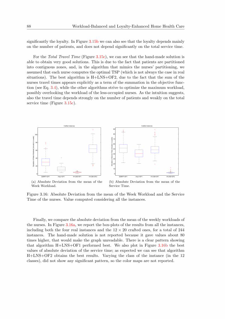
88 Workload-Balanced and Loyalty-Enhanced Home Health Care
significantly the loyalty. In Figure 3.15b we can also see that the loyalty depends mainlyon the number of patients, and does not depend significantly on the total service time.
For the Total Travel Time (Figure 3.15c), we can see that the hand-made solution isable to obtain very good solutions. This is due to the fact that patients are partitionedinto contiguous zones, and, in the algorithm that mimics the nurses’ partitioning, weassumed that each nurse computes the optimal TSP (which is not always the case in realsituations). The best algorithm is H+LNS+OF2, due to the fact that the sum of thenurses travel times appears explicitly as a term of the summation in the objective func-tion (see Eq. 3.4), while the other algorithms strive to optimize the maximum workload,possibly overlooking the workload of the less-occupied nurses. As the intuition suggests,also the travel time depends strongly on the number of patients and weakly on the totalservice time (Figure 3.15c).
0
20
40
60
80
100
GSRFF+OF1 Heur+OF1 H+LNS+OF1 H+LNS+OF2
Dev
iatio
n of
Wee
k W
orkl
oad
(min
utes
in a
wee
k)
Crafted instances
(a) Absolute Deviation from the mean of theWeek Workload.
0
10
20
30
40
50
60
70
80
90
GSRFF+OF1 Heur+OF1 H+LNS+OF1 H+LNS+OF2
Dev
iatio
n of
Ser
vice
Tim
e (m
inut
es in
a w
eek)
Crafted instances
(b) Absolute Deviation from the mean of theService Time.
Figure 3.16: Absolute Deviation from the mean of the Week Workload and the ServiceTime of the nurses. Value computed considering all the instances.
Finally, we compare the absolute deviation from the mean of the weekly workloads ofthe nurses. In Figure 3.16a, we report the box-plots of the results from all the instances,including both the four real instances and the 12 × 20 crafted ones, for a total of 244instances. The hand-made solution is not reported because it gave values about 80times higher, that would make the graph unreadable. There is a clear pattern showingthat algorithm H+LNS+OF1 performed best. We also plot in Figure 3.16b the bestvalues of absolute deviation of the service time; as expected we can see that algorithmH+LNS+OF2 obtains the best results. Varying the class of the instance (in the 12classes), did not show any significant pattern, so the color maps are not reported.

3.5 Conclusions 89
3.5 Conclusions
This chapter presents a real-life application of constraint solving technologies to theHome Health Care problem for the city of Ferrara, Italy. Our proposed Tailored La-grangian Metaheuristic has been included into a Constraint Programming frameworkusing a search algorithm based on Large Neighborhood Search.
The objectives, as requested by the chief nurses in charge of the service, were toprovide schedules with balanced workloads without increasing working hours and traveltimes, and to improve the service for the patients avoiding the unpleasant situation inwhich a patient is taken care by many different nurses. These objectives were obtainedthrough discussions with the chief nurses responsible for the service in Ferrara.
The results showed that the obtained solutions are significantly better under theserespects than the ones previously obtained by hand by the nurses. The use of CP wasconsidered a success; we decided to use it because of the ease of its use, and flexibilitywith respect to other techniques, such as Integer Programming. SAT and Answer SetProgramming (Brewka et al., 2011) are other interesting technologies to solve constrainedoptimization problems; modern solvers have sophisticated general-purpose search strate-gies, featuring restarts and nogood learning. CP, on the other hand, has powerful globalconstraints and allows the user to implement search strategies tailored for the givenproblem; in our experiments, custom search strategies had significantly better resultsthan general-purpose ones; however it would be interesting to compare with a SAT orASP solution.
The CP model has been implemented in Comet, which is more focused on the effi-ciency, and contains more global constraints, so we were able to propose a refined con-straint model adopting the multiknapsack and NV alue constraints, which can provideenhanced constraint propagation. Furthermore, we used a new search algorithm, basedon Large Neighborhood Search, that proved to be the most effective for this problem.
A deeper experimentation has been proposed with a set of crafted instances createdfrom data of the real instances, and show the Pareto front of the two main objectives.
Different objective functions have been studied. The first one is minimizing themaximum workload and the second one is minimizing the deviation of the workload.Both objective functions consider the traveling time and the loyalty. The first objectivefunction has reached better results.
Our proposed Tailored Lagrangian Metaheuristic has been used to calculate travelingtime for each nurse separately.
• Our Tailored Lagrangian Metaheuristic ensures the partial optimality of most so-lutions from the routing perspective. The reason is that, since we are consideringa relatively small number of patients per nurse, the proposed approach can quicklyfind the optimal solution to most TSP instances.
• We have compared our Tailored Lagrangian Metaheuristic respect ASP and Comettechnologies, obtaining that our proposed approach was the fastest.
• We also computed the percentage of time required by the Tailored Lagrangian

90 Workload-Balanced and Loyalty-Enhanced Home Health Care
Metaheuristic with respect to the rest of the solution process. We obtained that,in a typical run of the HHC solution process, it took less than 10% of the runningtime.

Part II:Asymmetric Problems


Chapter 4
Asymmetric Traveling SalesmanProblem
The Asymmetric Traveling Salesman Problem (ATSP) is a well-known NP-hard com-binatorial optimization problem. The ATSP is a variation of the TSP where the costmatrix is asymmetric, i.e., the time or distance to travel between two customers is de-pendent to the direction. The cost matrix can be represented by travel distance, time,fuel consumption or any other cost function between two locations. The cost matrixcan refer any of these terms interchangeably, but it is usually a function of the distancebetween pairs of locations.
As the TSP, it has numerous applications to different problems in logistics and man-agement, see Chapter 1. In real world applications, the usage of Euclidean or ortho-dromic distances are no valid. Mainly given that they do not represent the urban net-works, see Figure 4.1. For example, there might be a river, railroad or highway thatcould separate a city into zones, and vehicles are required to traverse bridges or spe-cific pathways. In real problems, the usage of Geographic Information Systems (GIS)and geo-spatial databases are crucial. Moreover, it’s worthy to distinguish that urbannetworks are asymmetric given that there are some one-way streets. Figures 4.1a-4.1bshows a representation of the effect of reversing the orientation of an urban route.
From the research point of view, the asymmetric TSP has been less studied thanthe symmetric TSP. For example, the number and size of benchmarks for the ATSP islimited, TSPLIB: ATSP benchmark (2008) has 19 instances, where the largest one is of443 nodes, and they commonly have random distance matrices with no plausible con-nection to real applications. There are some other less-known benchmarks, but offeringfewer or smaller instances. In addition, no single type of instance dominates the appli-cations of the ATSP, thus the experimental study of asymptotic behavior is much lessadvanced than in the case of the TSP. In the real-world context different researches havebeen created their own benchmarks. For example, 12 types of random instances weregenerated by Cirasella et al. (2001), and in the work of Rodrıguez and Ruiz (2012a),instances with 3 types of locations were generated calculating the distances with the aidof a GIS. Furthermore, some ATSP instances remain unsolved given that the number of
93

94 Asymmetric Traveling Salesman Problem
(a) Counterclockwise tour using asymmetriccosts obtained from GIS (17.7 km).
(b) Clockwise tour using asymmetric costs ob-tained from GIS (15.6 km).
(c) Tour obtained using symmetric costs calcu-lated with Euclidean distance (10.7 km).
Figure 4.1: Comparative of a tour in Barcelona according the symmetry or asymmetryof the distance cost.
researches on ATSP is much lower, and experimental studies of heuristics for the ATSPis less advanced.
Few of the algorithms designed to solve the symmetric TSP can be adapted to solvethe asymmetric problem. Some authors have been transformed the asymmetric matrixinto symmetric matrix, aiming to use their algorithms designed for solving the symmet-ric TSP. However, these transformations affect the efficiency of the methodology. Forinstance, the Concorde solver which was designed for solving the symmetric TSP, onlyworks with symmetric matrices and the transformation of matrices is the only possibleway of dealing with asymmetric problems. Rodrıguez and Ruiz (2012a) compare the

4.1 Problem Definition 95
effect of the asymmetry respect three different transformations, and conclude that thetransformation to solve ATSP problems is viable, but affects drastically the efficiency ofConcorde. In the work of Fischetti et al. (2003), it is compared Concorde with Branch-and-Cut methodology designed for the ATSP, and suggest that enriching the Concordearsenal of symmetric TSP separation tools by means of ATSP-specific separation proce-dures would be the road to go for the effective solution of hard ATSP instances.
Given all these motivations, we pretend to adapt our Tailored Lagrangian Meta-heuristic to the ATSP. In the next section, it is presented a literature review of theATSP without considering the works which perform matrix transformations.
4.1 Problem Definition
The Asymmetric Traveling Salesman Problem is a generalization of the TSP presented inChapter 1. Consider a complete graph, G(I, E), where I and E are the set of nodes andarcs, respectively. It assumes that the cost C is an asymmetric matrix that is cij 6= cjiin general, and then the complete graph G is directed. The asymmetric matrix cost Ccan represent the travel time, travel distance, travel cost, or a combination of them.
The ATSP goal, which is the same of the TSP, consists of determining the routewith minimum total traveling cost such that each customer is visited exactly once bythe salesman.
A well-known Integer Linear Programming formulation of ATSP is the following:∑i∈I
∑j∈I
cijxij (4.1)
subject to
∑i∈I
xij = 1 , ∀j ∈ I (4.2)∑j∈I
xij = 1 , ∀i ∈ I (4.3)
∑i∈S
∑j∈IrS
xij ≥ 1 , ∀ S ⊂ I : S 6= ∅ (4.4)
xij ∈ {0, 1} , i, j ∈ I (4.5)
In this formulation for the ATSP, O(n2) binary variables x are used. The binaryvariable xij indicates whether or not customer j is visited immediately after i. Theobjective function (4.1) aims to minimize the total cost of the route.
Every city node must be visited once and only once. From the point of view of theasymmetry, it means that every city must have one starting edge and one ending edge.Constraints (4.2) and (4.3) impose in-degree and out-degree of each vertex equal to one.

96 Asymmetric Traveling Salesman Problem
As well as the set of Subtour Elimination constraint (1.3) of the TSP, constraints(4.4) impose strong connectivity. Constraints (4.5) correspond exactly to equation (1.4)of the TSP, which impose integer variables.
Notice that the two constraints (4.2) and (4.3) could be replaced by∑
i∈I∑
j∈I xij =n, where n =| I | is the number of nodes. An interesting comparative of differentformulations for the ATSP problem can be found in the work of Oncan et al. (2009).
As the TSP, the ATSP is a NP-Hard problem and it can be formulated as findinga Hamiltonian circuit. The condition to ensure feasible solutions is that the directedgraph G must be strongly connected, and its underlying graph must be complete.
4.2 Literature Review
The best known exact algorithms for the ATSP are based on the Branch-and-Boundmethod which uses the well known Assignment Problem relaxation of the ATSP, fora complete description see (D. L. Miller & Pekny, 1991) and (Fischetti et al., 2007).Carpaneto et al. (1995) presented a lowest-first Branch-and-Bound algorithm to obtainexact solution of large-scale. They generated random instances with up to 2000 nodes,they also solved real-world stacker crane problems derived from a Siemens factory inAugsburg. Pekny and Miller (1992) presented a parallel Branch-and-Bound algorithmwhich is a parallelization of (Carpaneto & Toth, 1980), but improved with the appli-cation of the patching heuristic developed by Karp at the root node. Turkensteen etal. (2008) considered depth-first Branch-and-Bound algorithm. Their main algorithmiccontribution are the upper tolerance values of arcs in the corresponding AssignmentProblem instance to determine which arcs should be excluded, which is aiming to guidethe search for optimal solutions. Germs et al. (2012) developed a new tolerance-basedBranch-and-Bound algorithm proposing a lower bounding strategy with the expectedcosts of including arcs in the solution.
As state above, the Branch-and-Bound is the best known exact method, however, itis not the most effective exact method. Fischetti et al. (2007) surveyed exact methodsfor the ATSP and compared computationally Branch-and-Bound and Branch-and-Cutcodes. The results of this comparison proved that Branch-and-Cut is the most effectivemethod to solve hard ATSP instances. In the work of Fischetti and Toth (1997b), theauthors exploited additional classes of facet-inducing inequalities for the ATSP polytopethat proved to be of crucial importance for the solution of some real-world instances.Fischetti et al. (2003) compare the Branch-and-Cut algorithm by Fischetti and Tothwith Concorde, and conclude that it is generally better than Concorde. It was indicatedthe effectiveness of exploiting the ATSP-specific separation procedures. Moreover, thisBranch-and-Cut algorithm has been adapted to ATSP with time windows (Ascheuer etal., 2001) and ATSP with precedence constraints (Ascheuer et al., 2000).
Some classical heuristics for the ATSP are Nearest Neighbor, Nearest Insertion andMultiple Fragment (often referred to as Greedy) algorithms. In addition to this classicclass of tour construction heuristics, some of the latest heuristic approaches that arebeing studied to solve the ATSP are Lin-Kernighan heuristic, Patching heuristic, Ge-

4.2 Literature Review 97
netic algorithms, Memetic algorithms and Evolutionary algorithms. For a review andexperimental analysis of heuristics see (Johnson et al., 2007).
Lin-Kernighan heuristic (LK) is a local search algorithm based on re-arranging seg-ments of the tour. Lin and Kernighan (1973) proposed an effective heuristic for the TSP,which is based on a k-Opt procedure with k variable in each step. Some of the mostimportant adaptations for LK heuristic to the ATSP are Kanellakis and Papadimitriou(1980) and Helsgaun (2000). On the work of Helsgaun (2000), it is described a veryeffective implementation of the LK, named LKH, for both symmetric and asymmetricproblems.
The second class to be considered are Cycle-Patching algorithms which are based onpatching together the cycles in a minimum cycle cover, it can be computed as the solutionto an Assignment Problem. The Patching heuristic was proposed by Karp (1979), hisheuristic has been extensively used to find an initial solution or upper bounds in Branch-and-Bound algorithms and hybrid methodologies. In the work of Glover et al. (2001),the Patching heuristic is modified joining two shortest cycles together, it tries all possiblepairs using the best one. They also described an algorithm combining their modifiedPatching heuristics with a recursive Path Contraction heuristic.
Genetic algorithms are a population-based approach for heuristic search in opti-mization problems, in our case for the ATSP, Nagata and Kobayashi (1997) proposedthe use of an edge assembly crossover operator for both cases, the symmetric and theasymmetric. Later, Nagata and Soler (2012) designed an effective crossover operatorfor the ATSP, experimental results demonstrate that their proposed Genetic algorithmoutperforms state-of-the-art heuristic algorithms and, in addition, they created a newset of benchmarks for the ATSP. In the work of Xing et al. (2008), it is proposed ahybrid approach which incorporates an improved Genetic algorithm and some optimiza-tion strategies that contribute to its effectiveness, both the crossover operation and themutation operation are improved by selecting the optimum from a set of solutions.
Some authors have improved the Genetic algorithm combining it with a local search,this approach is named Memetic algorithm, for an introduction see (Neri et al., 2012).The approach proposed by I. C. Choi et al. (2003) extends the Genetic algorithm searchspace by purposefully generating and including infeasible solutions in the population.Freisleben and Merz (1996) introduced a new recombination operator called the DistancePreserving Crossover and employed the 3-opt variant as a local search engine for theATSP. Later, Merz and Freisleben (1997) improved their results by adding a variantof the 4-opt move to the search in the ATSP cases. According to Buriol et al. (2004),based on the computational results reported for this method, one can say that a goodimplementation must combine several essential features: (i) suitable recombination andmutation operators; (ii) a fast and effective local search algorithm; (iii) a hierarchicallystructured population; (iv) suitable data structures and smart codification mechanisms.In their work, all of the four key features are incorporated responsibly for an effectivesolution.
Evolutionary algorithms seek to solve search problems by modeling the behaviorsof social insects such as bees and ants. Ant Colony Optimization is not only capable

98 Asymmetric Traveling Salesman Problem
of generating good solutions for the symmetric TSP, but also for asymmetric instancesof the TSP, it was first initially proposed by Dorigo and Gambardella (1997). In thework of Andziulis et al. (2011), it is compared an Ant Colony Optimization with theNearest Neighbor heuristic using specific real-life instances. Their conclusions suggestthat the Ant Colony Optimization algorithm obtains better results, but it is slightlyslower. Bai et al. (2011) proposed parallel optimization architecture in which a Branch-and-Bound and a Ant Colony Optimization are launched concurrently, and a reductionprocedure takes useful information from both solver to reduce the global search spaceand hence speed up the rate of convergence to optimality. In Wong et al. (2013), theauthors presented a generic Bee Colony Optimization framework, which computationallyrealizes the bee foraging behavior in a typical bee colony where bees travel across differentlocations to discover new food sources and perform waggle dances to recruit more beestowards newly discovered food sources. Celik and Ulker (2012) proposed a Marriage inHoney Bee Optimization which is a meta-heuristic procedure inspired by the mating andinsemination process of honey bees.
A quite recent method to solve VRPs is the Variable Neighborhood Search, it wasintroduced for the first time by Mladenovic and Hansen (1997). Burke et al. (2001)presented effective new local and Variable Neighborhood Search heuristics for the ATSP,they introduced a local search routine based on splitting the original problem into smallsubproblems which are then solved to optimality using an exact algorithm.
The Lagrangian Relaxation (LR) is a well studied method, for a good survey on LRfor solving the ATSP see Rocha et al. (2004). Balas and Christofides (1981) proposeda Restricted Lagrangian Relaxation for the ATSP based on the Assignment Problem.They developed an LR approach by relaxing the subtour elimination constraints. Inaddition, it is generated upper bounds using a fast tour-building heuristic. Once thebound-strengthening techniques have been exhausted without matching the upper withthe lower bound, they branch by using two different rules, according to the situation:the usual subtour breaking disjunction, and a new disjunction based on conditionalbounds. In the work of Smith (1980), it is used an 1-Arborescence relaxation, in whichthe out-degree constraints are relaxed, and developed a Lagrangian method based on thisrelaxation to provide lower bounds for a Branch-and-Bound method. (Fischetti & Toth,1992) devoted much more computational effort to improve the bound of the Assignmentproblem relaxation. It was used a fairly complex additive bounding procedure solving adifferent relaxation of the ATSP at each iteration with costs given by the residual costfrom the previous iteration. They used the Restricted Lagrangian Relaxation proposedby Balas and Christofides. In Asadpour et al. (2010), it is considered the LagrangianRelaxation of the ATSP based on the Spanning Arborescence of minimum weight. Theyfirst constructed a spanning tree with special properties. Then they find a minimum costEulerian augmentation of this tree, and finally, shortcut the resulting Eulerian walk.

4.3 Our proposed TLM for the asymmetric case 99
4.3 Our proposed TLM for the asymmetric case
In this section, our Tailored Lagrangian Metaheuristic for solving the TSP is adaptedto the ATSP. For this problem, the out-degree constraints are relaxed, then the dualproblem obtained is an 1-Arborescence, that is, the directed analog of the 1-Tree problem.In order to adapt our TLM, Edmond’s Algorithm is used to solve the dual problem, anda new heuristic to obtain a feasible solution from a dual one is proposed.
The remainder aspects about our TLM is as proposed in Algorithm 3 on page 35,specially our main contribution consists on the new parameter which is updated usingthe values of both UB and LB and has improved significantly algorithm’s convergenceon the optimal solution.
Modeling the Lagrangian Dual Problem
The Subtour Elimination constraint (4.4) and the in-degree constraint (4.2) can be dis-regarded solving x as an 1-Arborescence. Then, the complicated set of constraints is theout-degree constraints (4.3).
A Spanning Arborescence is the directed graph form of a rooted tree, that is, for anode r called the root, there is exactly one directed path from r to any other node. Aminimum Spanning Arborescence can be calculated easily, for example, the order of Ed-monds’ Algorithm is O(EI). Therefore, the 1-Arborescence is a Spanning Arborescenceplus an additional incoming edge to the root, and thus, it has only one cycle in it.
In this proposed approach to the ATSP, LR relaxes the constraint set requiring thatall customers must have one out going edge, as proposed by Smith (1980). Therefore,the Lagrangian Dual problem obtained from ATSP by taking into the objective functionthe inequalities 4.3 is as follows:
maxu∈RN
L(u) (4.6)
where
L(u) = minx 1−Arborescence
(∑i∈I
∑j∈I
xijcij +∑i∈I
ui(1−∑j∈I
xij))
=
=∑i∈I
ui + minx 1−Arborescence
(∑i∈I
∑j∈I
(cij − ui)xij)
=
=∑i∈I
ui + minx 1−Arborescence
∑i∈I
∑j∈I
cijxij (4.7)
where cij = cij − ui define the dual cost.Its subgradient γ represents the penalization of the outgoing edges being a vector of
dimension n, calculated as follows:
γ = 1−∑j∈I
xij (4.8)

100 Asymmetric Traveling Salesman Problem
The dual solution is an optimal solution of the ATSP if and only if
‖ γ ‖2= 0 (4.9)
Edmonds’ Algorithm
Considering a directed graph G(I, E), where I and E are the set of nodes and arcs,respectively. Let |I| = n. The Spanning Arborescence problem consists on finding arooted directed spanning tree, G(I, S) where S is a subset of E of minimal cost. Therooted directed spanning tree is defined as a connected graph with n− 1 arcs, i.e., eachnode, except the root, has one incoming arc without any cycle.
Algorithm 8 Edmonds’ Algorithm for the 1-Arborescence
Initialization:Let be the subset S = ∅ ⊂ E.Discard the incoming edges to the depot.
for each node other than the depot doSelect the incoming edge e with the smallest cost.Add this edge to the subset: S = S ∪ {e}.
end forwhile G(I, S) contains a cycle do
for each cycle Ck formed doContract the nodes in the cycle Ck into a pseudo-node k.Modify the cost of each edge which enters a node j in the cycle from some nodei outside the cycle according to the equation 4.10.
end forfor each pseudo-node k do
Select the entering edge which has the smallest modified cost.Replace the edge which enters the same real node in S by the new selected edge.
end forend while
Find e = (i, 1) ∈ E the minimal weighted edge entering to the depot with (1, i) /∈ S.Add this edge to the subset: S = S ∪ {e}.return S.
The main idea of Edmonds’ algorithm is to find a replacing edge which has theminimum extra cost to eliminate a cycle if any. For that, a pseudo-node is created withassociated cost according to the following equation representing the associated extra costto eliminate the cycle.
ci,k = minj∈Ck
{ci,j − cx(j),j + ck} (4.10)
where i is a node outside the cycle, j is a node in the cycle, cx(j),j is the cost of the edgein the cycle which enters j and ck is the minimum cost of all the edges entering to the
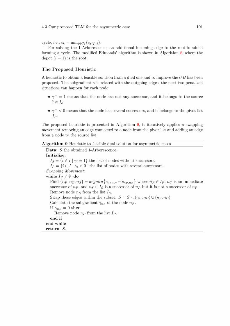
4.3 Our proposed TLM for the asymmetric case 101
cycle, i.e., ck = minj∈Ck{cx(j),j}.
For solving the 1-Arborescence, an additional incoming edge to the root is addedforming a cycle. The modified Edmonds’ algorithm is shown in Algorithm 8, where thedepot (i = 1) is the root.
The Proposed Heuristic
A heuristic to obtain a feasible solution from a dual one and to improve the UB has beenproposed. The subgradient γ is related with the outgoing edges, the next two penalizedsituations can happen for each node:
• γ− = 1 means that the node has not any successor, and it belongs to the sourcelist IS .
• γ− < 0 means that the node has several successors, and it belongs to the pivot listIP .
The proposed heuristic is presented in Algorithm 9, it iteratively applies a swappingmovement removing an edge connected to a node from the pivot list and adding an edgefrom a node to the source list.
Algorithm 9 Heuristic to feasible dual solution for asymmetric cases
Data: S the obtained 1-Arborescence.Initialize:IS = {i ∈ I | γi = 1} the list of nodes without successors.IP = {i ∈ I | γi < 0} the list of nodes with several successors.
Swapping Movement:while IR 6= ∅ do
Find {nP , nC , nS} = argmin{cnS ,nC − cnP ,nC
}where nP ∈ IP , nC is an immediate
successor of nP , and nS ∈ IS is a successor of nP but it is not a successor of nP .Remove node nS from the list IS .Swap these edges within the subset: S = S r (nP , nC) ∪ (nS , nC)Calculate the subgradient γnP of the node nP .if γnP = 0 then
Remove node nP from the list IP .end if
end whilereturn S.
102 Asymmetric Traveling Salesman Problem
4.4 Computational Results
Our TLM methodology adapted for the ATSP in this chapter has been implemented inJava language. All tests have been performed on a personal laptop with an Intel Corei5 processor at 2.40GHz and 4GB RAM.
A total of 27 ATSP instances have been used to test the efficiency of the proposedapproach. They have been obtained from the library TSPLIB (http://www.iwr.uni-heidelberg.de/groups/comopt/software/TSPLIB95/atsp/ last updated August 6,2008), a reference site with a large number of instances for the TSP, and related problems,from various sources and of various types.
The experiments have been conducted using the distance according to the specifi-cation included in the library, and using the next values for the parameters: 300 thenumber of iterations; δ0 = 1.99; ρ = 0.95 and αL = 2/3.
Table 4.2 shows results obtained for all 27 instances from the selected benchmarksets; and each of these results are compared to the best known solutions (BKS) so far.The table summarizes information regarding the best lower bound (LB, i.e, the bestdual value), the percentage distance from BKS of the LB (%∆LB), the best feasiblesolution found (UB), the percentage distance from BKS of the UB (%∆UB), and thefinal CPU time in seconds (tFinal).
The methodology has found the optimal value in four instances, in these cases, thenumber of iteration when it stopped is shown inside brackets in the last column. Notethat in two cases, the metaheuristic does not recognize the optimal value without stop-ping until the last iteration is reached. The table shows that the gap is kept reasonablylow for most of the considered instances, however, it does not succeed for all instancesbeing the average gap 2.43 %.
Furthermore, symmetric TSP instances are used to compare if this adaptation forthe asymmetric case is as good as the original TLM for the symmetric case. Tables4.3–4.4 provide a comparison between both proposed algorithms for 33 symmetric TSPinstances. The first results correspond to the original TLM for the TSP, presented inChapter 1. And the second results correspond to this adaptation for the ATSP.

4.4 Computational Results 103
# Nodes BKS LB %∆LB UB %∆UB CPUtime (s)
br17 17 39 38.99 0.03 % 40 2.56 % 0.59p43 43 5620 1025.32 81.76 % 5627 0.12 % 1.60ry48p 48 14422 14288.87 0.92 % 14422 0.00% 1.83 (Max it)ft53 53 6905 6905.00 0.00 % 6905 0.00% 1.51 (it 258)ft70 70 38673 38651.04 0.06 % 38802 0.33 % 3.06ftv33 34 1286 1286.00 0.00 % 1286 0.00% 0.28 (it 140)ftv35 36 1473 1457.28 1.07 % 1475 0.14 % 0.61ftv38 39 1530 1514.26 1.03 % 1532 0.13 % 0.73ftv44 45 1613 1584.46 1.77 % 1648 2.17 % 1.04ftv47 48 1776 1747.93 1.58 % 1810 1.91 % 1.50ftv55 56 1608 1583.63 1.52 % 1632 1.49 % 2.10ftv64 65 1839 1807.15 1.73 % 1858 1.03 % 2.60ftv70 71 1950 1907.96 2.16 % 1965 0.77 % 3.58ftv90 91 1579 1569.46 0.60 % 1579 0.00% 7.72 (Max it)ftv100 101 1788 1766.78 1.19 % 1851 3.52 % 9.58ftv110 111 1958 1922.67 1.80 % 2038 4.09 % 14.19ftv120 121 2166 2128.67 1.72 % 2266 4.62 % 16.73ftv130 131 2307 2284.52 0.97 % 2440 5.77 % 21.73ftv140 141 2420 2398.15 0.90 % 2527 4.42 % 25.92ftv150 151 2611 2589.82 0.81 % 2694 3.18 % 31.78ftv160 161 2683 2645.72 1.39 % 2759 2.83 % 41.13ftv170 171 2755 2713.96 1.49 % 2800 1.63 % 47.58kro124p 100 36230 35993.03 0.65 % 36682 1.25 % 11.90rbg323 323 1326 1206.22 9.03 % 1495 12.75 % 1464.93rbg358 358 1163 835.82 28.13 % 1275 9.63 % 2078.44rbg403 403 2465 1595.82 35.26 % 2484 0.77 % 888.30rbg443 443 2720 1750.80 35.63 % 2736 0.59 % 1211.06
7.90 % 2.43 %
Table 4.2: Results for 27 ATSP instances.

104 Asymmetric Traveling Salesman Problem
Ad
ap
ted
TL
Mfo
ras
ym
met
ric
case
sO
rigi
nal
TL
Mfo
rsy
mm
etri
cca
ses
BK
SLB
%∆LB
UB
%∆UB
CPUtime
(s)
LB
%∆LB
UB
%∆UB
CPUtime
(s)
eil5
142
6422.
380.8
5%
444
4.23
%2.
547
422.
420.
84%
440
3.29
%0.
226
st70
675
670.7
70.
63
%69
32.
67%
5.54
667
0.89
0.61
%68
71.
78%
0.25
5ei
l76
538
536.
740.2
3%
550
2.23
%6.
456
536.
940.
20%
544
1.12
%0.
297
pr7
610
8159
1050
99.8
22.8
3%
1103
802.
05%
6.70
510
5112
.85
2.82
%10
8584
0.39
%0.
25ra
t99
121
11205
.81
0.43
%12
402.
39%
14.1
2812
05.9
10.
42%
1237
2.15
%0.
257
kro
A10
0212
82
20928.
631.6
6%
2184
52.
65%
14.8
9320
930.
101.
65%
2131
90.
17%
0.43
2kro
B10
022
141
218
21.8
61.4
4%
2317
44.
67%
15.5
7921
830.
021.
40%
2293
13.
57%
0.26
7kro
C10
0207
4920
464.9
51.
37
%21
609
4.14
%15
.163
2046
7.78
1.36
%21
270
2.51
%0.
53kro
D10
021
294
21136.
740.7
4%
2201
43.
38%
15.4
8421
138.
270.
73%
2179
22.
34%
0.29
8kro
E100
2206
821
795
.27
1.24
%23
495
6.47
%15
.564
2179
8.00
1.22
%22
905
3.79
%0.
734
rd10
079
10
7897.4
10.1
6%
8240
4.17
%15
.385
7898
.65
0.14
%80
061.
21%
0.49
9ei
l101
629
627.
330.2
7%
641
1.91
%16
.071
627.
350.
26%
629
0.00
%0.
36li
n10
5143
791436
8.8
20.
07
%14
529
1.04
%17
.342
1437
0.14
0.06
%14
402
0.16
%0.
237
pr1
07
4430
3390
32.8
211
.90
%45
856
3.51
%20
.189
3931
3.79
11.2
6%
4442
00.
26%
0.37
9p
r124
5903
0580
40.0
41.6
8%
6144
94.
10%
28.4
3658
048.
181.
66%
6011
21.
83%
0.46
3b
ier1
2711
828
2117
381.
050.7
6%
1238
624.
72%
31.9
9111
7396
.83
0.75
%12
4502
5.26
%1.
404
ch13
0611
060
72.
110.6
2%
6351
3.94
%35
.601
6074
.46
0.58
%62
031.
52%
0.35
1p
r136
9677
2954
91.9
41.3
2%
1056
539.
18%
38.3
6895
373.
051.
45%
1025
345.
95%
0.90
5
1.57
%3.
75%
17.5
21.
52%
2.07
%0.
45
Tab
le4.
3:C
ompar
ison
bet
wee
nb
oth
pro
pos
edal
gori
thm
s,th
eor
igin
alT
LM
for
the
TS
Pan
dth
ead
apta
tion
for
the
AT
SP
,fo
r33
TS
Pin
stan
ces.

4.4 Computational Results 105
Adapte
dT
LM
for
asym
met
ric
case
sO
rigi
nal
TL
Mfo
rsy
mm
etri
cca
ses
BK
SLB
%∆LB
UB
%∆UB
CPUtime
(s)
LB
%∆LB
UB
%∆UB
CPUtime
(s)
ch150
6528
6487
.79
0.62
%67
032.
68%
52.4
6164
88.1
20.
61%
6640
1.72
%1.
279
kro
A150
2652
426
280.
770.
92%
2817
76.
23%
55.4
6326
280.
900.
92%
2759
84.
05%
1.60
8kro
B150
2613
025
716.
88
1.58
%28
137
7.68
%53
.733
2572
5.39
1.55
%27
273
4.37
%1.
577
pr1
5273
682
663
53.7
29.
95
%77
637
5.37
%57
.241
6658
3.97
9.63
%78
848
7.01
%0.
219
u15
942
080
4191
0.24
0.40
%43
702
3.85
%63
.464
4192
1.90
0.38
%42
636
1.32
%1.
186
rat1
9523
23229
0.07
1.42
%25
027.
71%
125.
598
2290
.58
1.40
%24
897.
15%
2.44
3kro
A200
2936
829
045.
961.
10%
3174
28.
08%
145.
176
2905
6.19
1.06
%30
983
5.50
%3.
231
kro
B200
2943
729
152.
20
0.97
%31
844
8.18
%13
6.54
929
158.
270.
95%
3112
65.
74%
2.96
ts22
512
6643
1154
63.1
18.
83
%14
0220
10.7
2%
189.
093
1154
72.0
98.
82%
1442
9913
.94
%1.
145
tsp22
539
1938
72.4
41.1
9%
4360
11.2
5%
216.
722
3875
.89
1.10
%42
618.
73%
3.23
pr2
2680
369
785
37.4
92.
28
%84
748
5.45
%20
7.97
7845
1.35
2.39
%84
203
4.77
%3.
155
gil2
6223
78235
1.62
1.11
%25
155.
76%
341.
253
2354
.00
1.01
%24
733.
99%
5.11
7pr2
6449
135
461
90.8
55.
99
%51
898
5.62
%34
6.00
246
236.
485.
90%
5086
83.
53%
5.18
a280
2579
2564
.48
0.56
%27
275.
74%
400.
3525
65.4
00.
53%
2704
4.85
%7.
202
pr2
9948
191
473
26.6
71.
79
%52
052
8.01
%52
4.62
4736
0.81
1.72
%51
053
5.94
%7.
86
2.58
%6.
82%
194.
382.
53%
5.51
%3.
16
Tab
le4.
4:(c
onti
nu
ed)
Com
par
ison
bet
wee
nb
oth
pro
pos
edal
gori
thm
s,th
eori
gin
al
TL
Mfo
rth
eT
SP
an
dth
ead
apta
tion
for
the
AT
SP
,fo
r33
TS
Pin
stan
ces.

106 Asymmetric Traveling Salesman Problem
Table 4.5 summarizes the results obtained in tables 4.3–4.4, the solved problems arepresented ordered by size. It may be observed that the adaptation for the asymmetriccase obtains almost as good as the original one. Particularly, the adaptation is notcomparable in terms of computational efficiency, see Figure 4.6.
Adapted TLM for asymmetric cases Original TLM for symmetric cases
Size Problems %∆UB CPUtime (s) %∆UB CPUtime (s)
n < 150 18 3.75 % 17.52 2.07 % 0.45150 ≤ n < 300 15 6.82 % 194.38 5.51 % 3.16
Table 4.5: Summary of results obtained comparing both algorithms for 33 TSP instances.
0
100
200
300
400
500
600
CP
Utim
e (s)
Compare both algorithms for TSP instances
eil5
1
st70
eil7
6pr
76ra
t99
kroA
100
kroB
100
kroC
100
kroD
100
kroE
100
rd10
0ei
l101
lin10
5pr
107
pr12
4bi
er12
7ch
130
pr13
6ch
150
kroA
150
kroB
150
pr15
2u1
59ra
t195
kroA
200
kroB
200
ts22
5ts
p225
pr22
6gi
l262
pr26
4a2
80pr
299
adapted TLR for asymmetric casesoriginal TLR for symmetric cases
Figure 4.6: Comparison of CPUtime between both proposed algorithms, the originalTLM for the TSP and the adaptation for the ATSP, for 33 TSP instances.
4.5 Conclusions
This chapter has presented an adaptation of our proposed Tailored Lagrangian Meta-heuristic for solving the Asymmetric Traveling Salesman Problem.
Our method uses the Subgradient algorithm combined with a heuristic which isintroduced to obtain a feasible solution from the dual variable providing both UB andLB, thus a posterior quality check of the solution is obtained. The motivation of ourmethod is the common sense belief that dual solutions could be relevant to primalsolutions.

4.5 Conclusions 107
The results have shown that the new parameter has improved significantly Subgra-dient’s convergence on the optimal solution and it is showing good results in terms ofthe quality of the solution. However, it is not showing a good behavior in terms ofcomputational efficiency.


Chapter 5
Asymmetric Capacitated VehicleRouting Problem
The Vehicle Routing Problem (VRP) is a flourishing research area with clear applica-tions to real-life distribution companies. VRPs deal with the physical distribution ofgoods from a central depot to customers, see for instance Toth and Vigo (2002a) andGolden et al. (2008). The best-known VRP variant is the so-called Capacitated Vehi-cle Routing Problem (CV RP ). However, frequent assumption is that distance-basedcosts associated with traveling from one node i (customer or depot) to another node j,cij , are symmetric, i.e., cij = cji for all pair of nodes. This assumption is not alwaysreasonable in real-life scenarios. It should also be taken into account that the maingoal of VRPs is to minimize distance-based costs associated with the distribution ofproducts among customers while satisfying customers‘ demands. To contribute closingthis gap between theory and practice, we propose a hybrid methodology for solving theAsymmetric Capacitated Vehicle Routing Problem (ACVRP).
In the VRP is common to consider a matrix which elements are the individual costs oftraveling from one node to another. These costs can be based on several distance-relatedfactors, such as: actual distance, time employed, fuel consumption, etc. In fact, classicalbenchmark instances are based on Euclidean distances between each pair of locations,which results in symmetric costs. However, this metric is just a lower bound of the realdistance between two nodes connected by a transport network or highway. The realdistance will depend upon the specific location of the nodes in the territory and also onthe structure of the road network that communicates them. Moreover, when consideringoriented networks, real distances might not have to be symmetric (Rodrıguez & Ruiz,2012b).
This chapter aims to present an efficient and relatively easy-to-implement method-ology for solving the Asymmetric Capacitated Vehicle Routing Problem (ACVRP). Ourapproach is based on the combination of a randomized version of a classical heuristicwith several local search processes specifically adapted to deal with the asymmetric na-ture of costs. The approach presented in this chapter was first presented in (Herrero etal., 2014).
109
110 Asymmetric Capacitated Vehicle Routing Problem
5.1 Problem Definition
In general, VRP problems are NP − complete within the combinatorial optimizationfield. Its constraints make it difficult to find feasible and good solutions in a reasonablecomputing time.
The ACVRP goal is the same of the CVRP, see Chapter 2. Solving the ACVRPconsists of determining the set of minimum k ≤ K routes with minimum total travelingcost and such that each customer is visited exactly once by a single vehicle, each routestarts and ends at the single-depot, and the total demand of the customers assigned toa route does not exceed the vehicle capacity Q. The only difference from the CVRP isthe asymmetry of the distance matrix.
Let G = (I, E) be a complete and directed graph, where I = {0, 1, . . . , n} is the setof nodes and E is the set of arcs. The nodes i = 1, 2, . . . , n correspond to customers,each with a deterministic demand di ≥ 0. The node i = 0 is the depot with zero-demandd0 = 0. Let K > 0 be the number of available vehicles, all of them with the same loadcapacity Q > 0. Let cij be the non-negative distance-based cost associated with the arc(i, j) ∈ E, and cii = +∞, ∀i ∈ I. The distance matrix is considered asymmetric, thatmay be calculated using the real distances between pairs of locations (i, j), i.e., it canhappen that cij 6= cji.
The first formulation of this problem was proposed by Laporte et al. (1986). Awell-known programming formulation of the problem is presented as follows:
min∑i∈I
∑j∈I
cijxij (5.1)
subject to: ∑i∈Ir{j}
xij = 1 ∀j ∈ I r {0} (5.2)
∑j∈Ir{i}
xij = 1 ∀i ∈ I r {0} (5.3)
∑i∈Ir{0}
xi0 ≤ K (5.4)
∑i∈Ir{0}
xi0 =∑
j∈Ir{0}
x0j (5.5)
∑i∈Ir{j}
yij + dj =∑i∈I
yji ∀j ∈ I r {0} (5.6)
0 ≤ dixij ≤ yij ≤ (Q− dj)xij ∀(i, j) ∈ E (5.7)
xij ∈ {0, 1} ∀(i, j) ∈ E (5.8)
yij ∈ [0, Q] ∀(i, j) ∈ E (5.9)
In this formulation for the ACVRP, O(n2) binary variables x are used. The binaryvariable xij in (5.8) indicates whether or not customer j is visited immediately after i.
5.2 Literature Review 111
In addition, there are O(n2) variables y, defined in Equation (5.9), where yij representsthe load in the truck arriving at customer j after visiting customer i in terms of unitsof commodity.
The objective function (5.1) minimizes the total distance-based cost of the arcs usedby all routes generated. Constraints (5.2) and (5.3) require that each customer is visitedexactly once, having one starting edge and one ending edge. Constraint (5.4) imposesthat the number of used vehicles does not exceed the number of available vehicles.Constraint (5.5) implies that the number of vehicles leaving the depot is the same as thenumber of vehicles returning to it.
Constraints (5.6) state that the quantity of products yij in the truck leaving customerj plus the demand of that customer, equals the quantity of products in the truck leavingit after the service has been completed. Constraints (5.7) guarantee lower and upperbounds ensuring that: the quantity of products yij in the truck leaving customer i isequals to or greater that its demand, di; and the total demand served by each vehicledoes not exceed the load capacity Q.
5.2 Literature Review
As described in (Laporte & Nobert, 1987) and also in (Toth & Vigo, 2001), there isa wide range of algorithms for solving the classic CVRP problem –exact algorithms,classical heuristics, and meta-heuristics. However, most techniques have been focusedon solving the symmetric CVRP.
It is much less common to find articles that focus exclusively on the asymmetricCVRP. In (Laporte et al., 1986) an exact algorithm is presented using the Branch-and-Bound method where the subproblems are a modified Assignment Problem. (Fischetti etal., 1994) propose a Branch-and-Bound algorithm using a new heuristic, named AV, ex-plicitly tailored for ACVRP, and its practical application to a real case of pharmaceuticaldistribution in a city of Italy.
In (Vigo, 1996), the author discusses the extension to the ACVRP of two of the mostimportant and successful techniques for the symmetric case: the Savings algorithm ofClarke and Wright (1964), and the optimization method of Fisher and Jaikumar (1981).The author states that the solutions found using the proposed asymmetric version ofthe Clarke-and-Wright Saving algorithm quickly evolves to worse values as the numberof customers increases, in addition to the inconvenience of the parameter combinationfor the parametric saving function. Furthermore, the author concluded that the newheuristic AV proposed in (Fischetti et al., 1994) is able to bluid a feasible solution betterthan those that can be obtained with the other algorithms from the literature.
More recently, there are two promising techniques that have been shown to work wellin both cases of symmetrical and asymmetrical CVRP. The first is a general heuristicproposed by (Pisinger & Røpke, 2007) which is the result of a unified heuristic for severalvariants of VRP using the Adaptive Large Neighborhood Search (ALNS). The second isa Memetic Algorithm (MA) described in (Nagata, 2007). These algorithms have beenselected by their performance and recognition. We have striven for a balance between

112 Asymmetric Capacitated Vehicle Routing Problem
simple classical techniques and also current and state-of-the-art methods.
Moreover, (De Franceschi et al., 2006) presented a ILP-based refinement heuristic forCVRP variants, for both symmetric and asymmetric costs, and for both with/withoutdistance constraints. They extended the refinement procedure proposed by Sarvanov andDoroshko (1981) for the TSP, and a procedure is involved to generate a large number ofnew sequences through the extracted nodes, as well as a more sophisticated ILP modelfor the reallocation of some of these sequences. In Pessoa et al. (2008), the authorsproposed a robust Branch-Cut-and-Price algorithm for the ACVRP that was also shownto be effective on a number of related problems. In particular, the use of cuts definedover the extended formulation seems very promising and deserves further development.
5.3 The SR-GCWS-CS algorithm adapted for the ACVRP
Constructive Component
The proposed algorithm is based on the randomized Clarke and Wright Savings algorithm(SR-GCWS-CS), developed by Juan et al. (2010); ? (?). The Clarke and Wright Savingsheuristic (CWS), presented by Clarke and Wright (1964), is one of the most commonlycited methods in the VRP literature. It uses the concept of savings associated with eacharc for merging routes. At each step, the arc with the greatest savings is selected if andonly if the two corresponding routes can be combined into a new feasible route and ifthe selected arc is composed of nodes that are directly connected with the depot. Weaddress the AVRP without considering an extensive asymmetric saving list –i.e., a listincluding two directed arcs for each pair of customers. Instead we consider a weightedsavings list considering just one arc for each pair of customers. Also, we consider thedirection of the resulting route after each merging.
Algorithm 10 offers a high-level view of our algorithm, where lines 3, 10 and 11 areessential for asymmetric problems. Our approach starts solving the problem as proposedin the CWS heuristic –i.e.: computing a dummy solution assigning one round-trip routefrom the depot to each customer. Then the algorithm computes the weighted savingslist using an auxiliary parameter β (see below the formulas for weighted saving, i.e.,Sij , and CWS saving, i.e., Sij). At this point the CWS heuristics is combined witha randomization process. We use a pseudo-geometric distribution to assign a selectionprobability to each edge in the savings list (alpha). Moreover, this selection probabilityis coherent with the weighted saving value associated with each edge, i.e., edges withhigher savings will be more likely to be selected from the list than those with lowersavings. Therefore, each combination of edges has a chance of being selected and mergedwith previously built routes. Then, a multi-start process is initiated and controlled bya time parameter (maxTime). At each iteration of this process, different edges areselected using the aforementioned biased probability distribution. This allows obtainingdifferent outputs at each iteration. After merging, we improve the merged route applyingtwo promising local search processes. At the end, we apply a general local search to thewhole solution which is explained below.

5.3 The SR-GCWS-CS algorithm adapted for the ACVRP 113
Algorithm 10 SR-GCWS-CS algorithm for the Asymmetric case
1: Initialization:2: Compute initial dummy solution (Clarke & Wright, 1964).3: Compute weighted savingsList using new parameter β.4: repeat until MaxTime is consumed.5: Perform a biased randomization of savingsList using α (Juan et al., 2010).6: repeat until savingsList is empty.7: Extract the next edge from savingList.8: if both nodes are exterior, they belong to a two different routes and both9: routes’ load can be assigned to a vehicle (load ≤ Q).
10: Merge routes without considering orientation.11: Apply Asymmetric Local Search and Cache technique.12: end if13: end repeat14: Apply splitting-based local search using maxSplitter (Juan et al., 2011).15: Update the best found solution.16: end repeat
One important contribution of our approach is the fact that we consider a weightedsavings list merging two routes without taking into account directions at this initialstage. See an example in Figure 5.1. The application of a local search will help to definethe best direction. The weighted saving associated with an arc connecting customers iand j is defined as:
Sij = β ∗max{Sij, Sji}+ (1− β) ∗min{Sij, Sji}
where β ∈ [0.5, 1] and Sij = c0i + c0j − cij .
Figure 5.1: Merging routes R1 = {0, h, i, 0} and R2 = {0, k, j, 0} with different orien-tation into a route R = {0, h, i, j, k, 0}. The route R2 is reversed and some edges arechanged given that it is an urban area with some one-way streets.
The disregard of orientation is important given that an asymmetric savings list doesnot choose arcs which do not match their orientation established. For example, it rejects

114 Asymmetric Capacitated Vehicle Routing Problem
the routes in Figure 5.1 since they have different orientation. This reduces the solutionspace and worsens the general solution; even some obtained solutions are using a greaternumber of vehicles.
Given that the orientations are not considered, an original local search for the asym-metric context was created exploring the near solution space with few steps. It representsanother important contribution of our approach.
Asymmetric Local Searches
Once a merged route is obtained, two local searches are applied in order to explore thesolution space with few steps. The first local search procedure is the so called ReversingRoutes local search. This procedure intends to find an improvement in the order andorientation of the nodes. Given a merged route, we first try to sort the nodes in a moreefficient way. If a route is composed by more than four nodes, then we take each fournodes –i.e., (i, j, k, l)– and try to determine if a swapping of two middle-nodes couldimprove the cost –i.e., (i, k, j, l). After that, we try to reverse the order in which nodesare traversed.
A second local search, originally described in (Juan et al., 2011), is focused on check-ing if a given set of nodes already exists in a memory but with a better order of thenodes. The basic idea of this learning mechanism is to store in a cache memory thebest-known order to travel among the nodes that constitute one route. This cache isconstantly updated whenever a better order with a lower cost is found for a given setof nodes. At the same time, the routes contained in this cache are re-used wheneverpossible to improve newly merged routes.
Finally, once all edges in the saving list have been considered, the resulting solution isimproved through a Splitting local search method proposed in (Juan et al., 2011). Thecurrent solution is divided into disjoint subsets of routes; then, each of these subsetsare solved applying the same methodology described before during a given number ofiterations (maxSplitter). This tries to apply a “divide and conquer” approach sincesmaller instances could be easier to solve.
5.4 Computational Results
In order to validate our algorithm, we present the results of 20 AVRP instances compar-ing our results with those obtained using the Memetic algorithm (MA) of (Nagata, 2007)and the Adaptive Large Neighbourhood Search (ALNS) of (Pisinger & Røpke, 2007).
We have selected 20 public AVRP instances from the workbench presented in thework of Rodrıguez and Ruiz (2012b), details on these instances can be found in http://
soa.iti.es/files/Instances CVRP.7z. They have been generated with a realisticperspective and mathematical justification. The selection was made at random amongthe set of medium- and large-size instances (in terms of number of nodes). They have50 or 100 customers and are designed to employ a homogeneous fleet with the numberof vehicles ranging from 2 to 7. These instances consider large demands and vehicle

5.4 Computational Results 115
capacities, as well as random location of the nodes within intra-city areas. The depotmay be in the center of the area, those with ‘C’ in the second letter of the name, or arandom position, those with ‘A’. The intra-city instances were chosen given that theyrepresent a higher asymmetry degree. Rodrıguez and Ruiz (2012b) conclude that theseinstances affect in a statistically significant way the CPU time needed by some algorithmsand deteriorate the quality of the solutions obtained.
The algorithm described in this Chapter has been implemented as a Java application.An Intel QuadCore i5 at 3.2 GHz and 4 GB RAM was used to perform all tests, whichwere run over Windows XP.
For the 20 AVRP instances, we have used 10 random seeds (10 replicas), an elapsedtime of 1 minute (maxTime) for each seed, and 60 iterations for the splitting technique(maxSplitter). In order to perform a biased randomization of the weighted savingslist, a quasi-geometric distribution with a parameter α randomly selected in the interval[0.5, 0.10] was used; and the value chosen for the weighted saving was β = 0.6.
We have selected the following state-of-the-art AVRP methods in order to comparewith:
• General heuristic of (Pisinger & Røpke, 2007). It is a unified heuristic that worksfor several variants of routing problems and that uses an Adaptive Large Neigh-borhood Search (ALNS).
• Memetic algorithm of (Nagata, 2007) (MA). Similar to ALNS, MA is a very pow-erful and recent AVRP metaheuristic.
The previous algorithms have been selected by their performance and recognition.We have striven for a balance between simple classical techniques and current and state-of-the-art methods. Algorithms MA and ALNS were run from the original C++ codewhich was kindly provided by their respective authors. No code modification was carriedout and the methods were run according to their recommendations.
The MA algorithm of Nagata was executed with a parameter setting: Npop = 100,Nch = 30, 10 trials and 2 parents. Also ten runs with elapsed time of 1 minute wereexecuted for each instance. For the ALNS, only one run was executed for each instancewithout time limit.
The results of these tests are summarized in table 5.2, which contains the followinginformation for each instance: name of instance; number of nodes; number of vehicles;the best solution of 10 replicas of the MA, {1}; the ALNS solution, {2}; gap, expressedas a percentage value, between {1} and {2}; the time used for ALNS in seconds; ourbest solution found, OBS {3}; and gap between {1} and {3}.

116 Asymmetric Capacitated Vehicle Routing Problem
Inst
ance
#N
od
es#
Veh
icle
sM
A{1}
AL
NS{2}
gap{1}-{2}
tim
e(s
)O
BS{3}
gap{1}-{3}
G-A
-CA
A05
0150
237
0.26
370.
260.
00%
17.8
3370.2
60.0
0%
G-A
-CA
A05
0250
341
4.44
414.
440.
00%
13.3
0414.4
40.0
0%
G-A
-CA
A05
0350
444
4.69
444.
690.
00%
10.4
8444.6
90.0
0%
G-A
-CA
A05
0450
236
2.01
362.
010.
00%
17.9
5362.0
10.0
0%
G-A
-CA
A05
0550
339
5.78
395.
780.
00%
15.5
9398.4
70.6
8%
G-A
-CA
A10
0110
05
661.
8866
4.53
0.40
%43.0
3675.3
12.0
3%
G-A
-CA
A10
0210
05
621.
0662
2.67
0.26
%39.3
6625.8
20.7
7%
G-A
-CA
A10
0310
05
627.
2962
7.29
0.00
%42.2
3627.2
90.0
0%
G-A
-CA
A10
0410
06
681.
8968
1.89
0.00
%34.8
4686.2
50.6
4%
G-A
-CA
A10
0510
07
810.
9781
0.97
0.00
%29.0
3820.5
61.1
8%
G-C
-CA
A05
0150
237
6.62
376.
620.
00%
17.7
0376.6
20.0
0%
G-C
-CA
A05
0250
337
2.48
372.
480.
00%
13.3
1372.4
80.0
0%
G-C
-CA
A05
0350
440
4.30
404.
300.
00%
10.3
6404.3
00.0
0%
G-C
-CA
A05
0450
236
1.74
361.
740.
00%
17.8
4361.7
40.0
0%
G-C
-CA
A05
0550
338
6.73
386.
730.
00%
13.8
0386.7
30.0
0%
G-C
-CA
A10
0110
05
596.
5459
6.86
0.05
%40.8
3600.3
50.6
4%
G-C
-CA
A10
0210
05
578.
1557
8.15
0.00
%38.6
1583.3
90.9
0%
G-C
-CA
A10
0310
05
561.
0856
1.08
0.00
%41.1
3566.1
00.8
9%
G-C
-CA
A10
0410
06
660.
8166
0.81
0.00
%35.1
9664.1
40.5
0%
G-C
-CA
A10
0510
07
652.
0865
2.18
0.02
%28.6
3652.4
20.0
5%
0.04
%0.4
1%
Tab
le5.
2:C
omp
aris
onof
resu
lts
for
AV
RP
inst
an
ces.

5.5 Conclusions 117
Notice that the results obtained with our approach are quite competitive, showingan average gap of 0.41% with respect to (Nagata, 2007), which always obtains the bestresults. Our approach also found exactly the same solution (gap = 0.00%) for 10 out of20 instances. Notice that all three algorithms were run using the same computing timeand machine. The only difference is that our algorithm was codified in Java, which runsover a virtual machine and thus has a lower performance than a code implemented innative C/C++.
5.5 Conclusions
In this chapter, we have discussed the importance of taking into account asymmetriccosts in realistic Vehicle Routing Problems. Despite the fact that real-life distancesare frequently asymmetric –especially in urban transportation–, there is a lack of worksconsidering asymmetric distances. Accordingly, we have presented a hybrid algorithmfor solving the Asymmetric Capacitated Vehicle Routing Problem (ACVRP). This algo-rithm combines a multi-start randomized savings algorithm (SR-GCWS-CS) with twolocal search processes specifically adapted to the asymmetric nature of costs in real-lifescenarios.
A complete set of ACVRP tests have been performed to illustrate the methodologyand analyze its efficiency when compared with two state-of-the-art algorithms. Theresults show that our approach is able to produce competitive results for the ACVRPwhile, at the same time, it is much simpler to implement and requires less parameters–and fine-tuning efforts– than current state-of-the-art algorithms.


Chapter 6
Asymmetric and HeterogeneousVehicle Routing Problem
As explained in Chapter 5, the Vehicle Routing Problem (VRP) has clear applicationsto real-life distribution companies. This chapter focuses on the fact that most road-transportation companies own a heterogeneous fleet of vehicles. However, most VRP-related academic articles assume the existence of a homogeneous fleet of vehicles.
The diversity in the vehicles capacity of companies might be due to the fact thatdifferent customers and locations might require different types of vehicles, e.g.: narrowroads in a city, available parking spaces, vehicle weight restrictions on certain roads,etc. Another reason for owning vehicles with distinct capacities is the natural diversitythat arises when vehicle acquisitions are made over time. Accordingly, Ruiz et al. (2004)and Prive et al. (2006) state the importance of developing new vehicle routing methodsconsidering heterogeneous fleets. Some real-life applications of heterogeneous fleets areillustrated in (Golden et al., 2002). Examples of these are: urban waste collection,residential pickups and delivery of beverages, food and newspapers delivery, etc.
Several VRP variants have been extensively studied during the last decades (Laporte,2009). Different VRP variants incorporate different sets of realistic constraints –i. e.vehicle capacity, asymmetric cost, heterogeneous fleets, delivery time windows, servicepriorities, pickup and delivery options, etc. Despite the fact they are common situationsin real-life scenarios, the combination of heterogeneous fleets with asymmetric costs hasbeen rarely discussed in the existing literature.
The first goal of this chapter is to solve the Asymmetric and Heterogeneous VehicleRouting Problem (AHVRP), for that the proposed methodology presented in Chapter 5is adapted. Additionally, this chapter also analyzes how asymmetric routing costs varywhen slight deviations from the homogeneous fleet are considered, i.e., how marginalcosts/savings change when a few ’standard‘ vehicles in the homogeneous scenario aresubstituted by other vehicles with different loading capacity.
119

120 Asymmetric and Heterogeneous Vehicle Routing Problem
6.1 Problem Definition
This chapter is focused on a particular variant of the V RP family, called AsymmetricHeterogeneous Fleet Vehicle Routing Problem. The model used next is an adaptationof the models proposed by Baldacci et al. (2008) and Wen et al. (2010). Both assumesymmetric and different transportation costs for each type of vehicle, limited number ofvehicles, as well as additional fixed costs for using each type of vehicle.
The model of three sub-indexes is formulated as follows. LetG = (I, E) be a completeand directed graph, where I = {0, 1, . . . , n} is the set of nodes and E is the set of arcs.The nodes i = 1, 2, . . . , n correspond to customers, each with a deterministic demanddi ≥ 0. The node i = 0 is the zero-demand depot, i.e., d0 = 0. Let m > 0 be thenumber of different types of vehicles. For the kth type of vehicles (k = 1, 2, . . . ,m),let Ik = {1, 2, . . . , vk} be the set of vehicles of type k, with load capacity Qk > 0.Let cij be the non-negative distance-based cost associated with the arc (i, j) ∈ E, andcii = +∞, ∀i ∈ I. In the case of calculating the real distances between pairs of locations(i, j), the distance matrix may be asymmetric, i.e., it can happen that cij 6= cji.
The AHVRP goal is to find the set of minimum-cost round-trip routes, starting fromand ending at the depot, which satisfy all customers’ demands, visit each customer onlyonce, and do not exceed the load capacity of each type of vehicle.
min∑i∈I
∑j∈I
cij
m∑k=1
xijk (6.1)
subject to:∑i∈Ir{0}
xi0k =∑
j∈Ir{0}
x0jk ∀k ∈ {1, . . . ,m} (6.2)
m∑k=1
∑i∈Ir{j}
xijk = 1 ∀j ∈ I r {0} (6.3)
∑i∈Ir{h}
xihk =∑
j∈Ir{h}
xhjk ∀h ∈ I r {0},∀k ∈ {1, . . . ,m} (6.4)
∑j∈Ir{0}
x0jk ≤ vk ∀k ∈ {1, . . . ,m} (6.5)
∑i∈Ir{j}
yij + dj =∑
i∈Ir{j}
yji ∀j ∈ I r {0} (6.6)
0 ≤ di · xijk ≤ yij ≤ (Qk − dj) · xijk ∀(i, j) ∈ E,∀k ∈ {1, . . . ,m} (6.7)
xijk ∈ {0, 1} ∀(i, j) ∈ E,∀k ∈ {1, . . . ,m} (6.8)
In this formulation, for both symmetrical and asymmetrical issues, and for bothhomogeneous and heterogeneous fleet, O(n2K) binary variables x are used. The binaryvariable xijk in (6.8) indicates whether or not the arc (i, j) ∈ E is traveled by a vehicleof type k (k = 1, 2, . . . ,m). In addition, there are O(n2) variables y where yij represents
6.2 Literature Review 121
the load in the truck arriving at customer j after visiting customer i in terms of unitsof commodity.
The objective function (6.1) minimizes the total distance-based cost of the arcs usedby all m routes generated. Constraints (6.2) imply that the number of vehicles of eachtype leaving the depot is the same as the number of vehicles of that type returning toit. Constraints (6.3) and (6.4) require that each customer is visited exactly once, andthat the same type of vehicle k arrives and leaves each h customer location respectively.Constraints (6.5) impose that the number of used vehicles of each type does not exceedthe number of available vehicles of that type. Constraints (6.6) state that the quantityof products yij in the truck leaving customer j plus the demand of that customer, equalsthe quantity of products in the truck leaving it after the service has been completed.Constraints (6.7) guarantee lower and upper bounds ensuring that: the quantity ofproducts yij in the truck leaving customer i is equals to or greater that its demand, di;and the total demand served by each vehicle k does not exceed the load capacity Qk.
6.2 Literature Review
Many combinatorial problems consider more than one fleet of vehicles with differentcapacities. Since the first axis of our addressed rich problem is the asymmetric costsmatrix, the second axis is the Heterogeneous Fleet VRP (HVRP). The HVRP has beenquite studied in the literature. For instance, Baldacci et al. (2008) present a compre-hensive description of some of its most important variants. On this last study, we canappreciate how the research community has addressed the HVRP in different ways. First,considering either a limited or an unlimited number of available vehicles of each type.Second, considering fixed and/or variable costs associated with the use of each type ofvehicle. Each vehicle could have a fixed cost for using it in a trip as well as a variablecost that is the result of multiplying a coefficient by the distance of the assigned route,i.e., cijk1 6= cijk2 ∀i, j and ∀k1 6= k2. These costs used to be associated to each typeof vehicle. The combinations of the aforementioned parameters have created the mainHVRP families, known as:
• H1: Fleet Size and Mix VRP with fixed and variable costs where an unlimitednumber of vehicles is considered for minimizing the addition of using a specificvehicle and the variable distance.
• H2: Fleet Size and Mix VRP with only fixed costs where an unlimited number ofvehicles is considered for minimizing fixed cost of all used vehicles.
• H3: Fleet Size and Mix VRP with only variable costs where an unlimited numberof vehicles is considered for minimizing the variable distance of all routes.
• H4: Heterogeneous Fixed Fleet VRP with only variable costs where a limitednumber of vehicles is used to minimizing the variable cost.
• H5: Heterogeneous Fixed Fleet VRP with fixed and variable costs where a limitednumber of vehicles is used to minimizing both variable and fixed costs.

122 Asymmetric and Heterogeneous Vehicle Routing Problem
Study HVRP family Method
Golden et al. (1984) H0, H2 HeuristicsTaillard (1999) H0, F2, H4 Column Generation-based heuristicGendreau et al. (1999) H0, H2, H3 Tabu SearchWassan and Osman (2002) H0, H2, H3 Tabu SearchRenaud and Boctor (2002) H0, H2 Heuristic-basedLima et al. (2004) H0, H2 Memetic algorithmTarantilis et al. (2004) H0, H4 Threshold Accepting algorithmsE. Choi and Tcha (2007) H0, H1, H2,
H3Branch-and-bound
F. Li et al. (2007) H0, H4 Record-To-RecordPrins (2009) H0, H1, H2,
H3, H4Memetic algorithm
Imran et al. (2009) H0, H1, H3 Variable Neighborhood-basedheuristic
Liu et al. (2009) H0, H2 Genetic algorithmBrandao (2009) H0, H2, H3 Tabu SearchEuchi and Chabchoub (2010) H0, H4 Hybrid Tabu SearchX. Li et al. (2010) H0, H5 Adaptive Memory Programming
MetaheuristicBrandao (2011) H0, H3, H4 Tabu SearchPenna et al. (2011) H0, H1, H2,
H3, H4, H5Iterative Local Search with VariableNeighborhood Descent
Subramanian et al. (2012) H0, H1, H2,H3, H4, H5
Iterative Local Search with SetPartitioning
Table 6.1: Summary of published HVRP studies.
Notice that there are others HVRP branches considering constraints like Site-Dependent,Site-Road, etc. For instance, Prins (2002) considers that each vehicle can optionally per-form several trips using a savings-based heuristic but without any extra cost. The basicfamily (H0) consists in the natural condition of considering a heterogeneous fleet insideof the combinatorial problem.
The Rich VRP (RVRP) is a generalized variant of the VRP where several constraints,aspects or objectives functions are considered at the same time. Examples of constraintsand assumptions considered in RVRPs could be: multi-depot, periodic visits to clients,open routes, multi-products, time windows, etc. Drexl (2012) compiles some currentneeds on the RVRP field as well as a state-of-the-art of scientific research and commercialsoftware. In some studies like Prins (2002); Bolduc et al. (2006); Irnich (2008); Rieckand Zimmermann (2010); Oppen et al. (2010); Prescott-Gagnon et al. (2010); Vallejoet al. (2012) the variable and fixed costs are ignored when combined with other routingfeatures. In fact, Bolduc et al. (2006) is included with other papers in a Special Issue ofRich VRP Hartl et al. (2006). Tables 6.1 and 6.2 summarize the work done in severaltypes of HVRP. On its columns, we can appreciate the addressed HVRP families, the

6.2 Literature Review 123
applied methodology, as well as others routing constraints considered on each study.Also, the first table (6.1) presents papers exclusively dedicated to the HVRP, while thesecond table (6.2) shows papers related to RVRP where the HVRP is also consideredtogether with other constraints. Most of these works just include the heterogeneouscapacity of vehicles (H0) and not the related costs associated with each type of vehicle.Therefore, there is not a single way to include the HVRP feature in a RVRP.
To the best of our knowledge, there is not any published work on the AHVRP. Themost approximated ones are presented in Marmion et al. (2010); Pessoa et al. (2008).In the first study, the authors analyses the sensitivity of two classical neighborhoodsmethods for the AHVRP. Thus, they simulate a heterogeneous fleet assigning differentvariable costs to each vehicle, but the capacity remains unchanged. On Pessoa et al.(2008), the authors developed a set of robust Branch-Cut-and-Price algorithms for sev-eral VRPs. Some promising experiments are presented, but changes in the capacity offleets are not justified for the HVRP. More details about these two studies are discussedlater.
Study HVRP family Method Extra constraints
Bolduc et al.(2006)
H0 Heuristics Multi-period
Irnich (2008) H0 Local Search-Basedmetaheuristic
Multi-depots, and timewindows
Baldacci andMingozzi(2009)
H0, H5 MIP model with SetPartitioning
Site-dependent, andmulti-depots
Rieck andZimmermann(2010)
H0 MILP model Time windows, andsimultaneous delivery& pickup
Oppen et al.(2010)
H0 ColumnGeneration-based
Multi-products,multiple trips,precedence andinventory constraints
Prescott-Gagnon et al.(2010)
H0 Heuristics Multi-depots,intra-routereplenishments, timewindows, driver shiftsand optional customers
Vallejo et al.(2012)
H0 Memory-basedApproach with
Clustering
Time windows,multi-depots, andmulti-trip
Table 6.2: Summary of published Rich HVRP studies.

124 Asymmetric and Heterogeneous Vehicle Routing Problem
6.3 The SR-GCWS-CS algorithm adapted for the AHVRP
The algorithm we propose is an adaptation of our proposed Asymmetric SR-GCWS-CSalgorithm presented in Chapter 5. The Clarke and Wright Savings heuristic (CWS) is awell known method (Clarke & Wright, 1964). Our approach combines the randomizedClarke and Wright Savings algorithm (SR-GCWS-CS), developed by Juan et al. (2010,2011) for the CVRP, with the modified Clarke and Wright Savings heuristic, presentedby Prins (2002) for the HVRP.
Constructive Component
Algorithm 11 offers a high-level view of our algorithm. Being demonstrated the compe-tence of our algorithm 10 for the asymmetric case, for the AHVRP only lines 8–11 and13 are modified.
Our approach starts solving the problem as proposed in the CWS heuristic, i.e.,computing a dummy solution assigning one round-trip route from the depot to each cus-tomer. Then the algorithm computes the weighted savings list as proposed in Chapter 5.At this point, the CWS heuristics is combined with the randomization process proposedin (Juan et al., 2010). Then, a multi-start process is initiated and controlled by a timeparameter (maxTime). At each iteration of this process, different edges are selectedusing a biased probability distribution, this allows obtaining different outputs at eachiteration.
Addressing the heterogeneous fleet
Before merging, the validation of the capacity constraint in a heterogeneous fleet isaddressed as a vehicle-trip assignment. For this, an effective method based on CWSis employed, (Prins, 2002). In the work of Prins, the list of vehicles and the list ofroutes are sorted decreasingly by load capacity and accumulated demands respectively;after that, a temporary assignment between the two lists is searched. If a successfulmatch –including all previously routes plus the new desirable merged one– is found,then the capacity constraint is satisfied and the temporary assignment becomes final.Otherwise, the merge becomes unfeasible. If a situation arises in which the number ofroutes is greater than the number of vehicles, then new fictitious vehicles are assignedto the remaining routes. Notice that this vehicle assignment validation is made for eachpossible saving, increasing the computational operations. However, in our approach itis not considered the assumption regarding that the largest demand cannot exceed thecapacity of the smallest vehicle.
After merging the routes and assigning vehicles, the Asymmetric Local Searches ex-plained in Section 5.3 is applied. Notice that it does not search a new vehicle assignment,the previously assigned vehicle to each route remains unchanged during this process.
Finally, once all edges in the saving list have been considered, the resulting solutionis improved through a Splitting local search method proposed in (Juan et al., 2011). Thecurrent solution is divided into disjoint subsets of routes together with their previously

6.4 Experimental Design 125
Algorithm 11 The Asymmetric SR-GCWS-CS for Heterogeneous Fleets
1: Initialization:2: Compute initial dummy solution (Clarke & Wright, 1964).3: Compute weighted savingsList using β.4: repeat until MaxTime is consumed.5: Perform a biased randomization of savingsList using α (Juan et al., 2010).6: repeat until savingsList is empty.7: Extract the next edge from savingList.8: if both nodes are exterior and they belong to a two different routes.9: Compute decreasing sorted list of vehicles and decreasing sorted list of
10: routes loads (Prins, 2002).11: if all routes’ load can be assigned to a candidate vehicle (load ≤ Qk).12: Merge routes without considering orientation.13: Assign final vehicles.14: Apply Asymmetric Local Search and Cache technique.15: end if16: end if17: end repeat18: Apply splitting-based local search using maxSplitter (Juan et al., 2011).19: Update the best found solution.20: end repeat
assigned vehicles; then, each of these subsets are solved applying the same methodologydescribed before during a given number of iterations (maxSplitter). This tries to apply a“divide and conquer” approach since smaller instances could be easier to solve. So a newset of routes could be created on each partition with the previously assigned vehicles.
6.4 Experimental Design
The most commonly-used methodology to compare the performance of different algo-rithms for solving VRPs consists in running these algorithms over a set of well-definedbenchmark instances. In the case of the CVRP or the AVRP, several benchmark setsare available through open-access websites, so that researchers worldwide can use them.Usually, these data sets contain complete information, including not just the instanceinputs and the best-known value for the objective function, but also a complete descrip-tion of the corresponding solution –i.e., the specific composition of each route in thebest-known solution. In the case of the AHVRP, however, there is not a commonly-accepted set of instances to test algorithms, since the AHVRP has rarely been discussedso far in the literature.
For the AHVRP, (Fischetti et al., 1994) developed some preliminary experimentsbased on a set of real AVRP instances. Likewise, (Marmion et al., 2010) analyzed theuse of a heterogeneous fleet. However, these studies have only considered the effect of

126 Asymmetric and Heterogeneous Vehicle Routing Problem
variable cost on vehicles selection, but no differences in actual vehicle capacities areconsidered. Also (Pessoa et al., 2008) have used these benchmarks first modifying thecapacity of the original fleets and then running the experiments with homogeneous fleets.
Therefore, we propose to extend, for the AHVRP, the 20 selected ACVRP instancesfrom http://soa.iti.es/files/Instances CVRP.7z, used in Chapter 5. We proposeto use exactly the same nodes of this ACVRP instances, including their asymmetric costsand demands, and the same number of vehicles. We then consider a heterogeneous fleetcomposed of ‘standard’ vehicles –i.e., vehicles with the capacity defined in the ACVRPinstances– and ‘non-standard’ vehicles with modified capacities. In our opinion, this isa natural way to adapt the homogeneous-capacity instances, since it allows the decision-maker to answer sensitivity-analysis questions such as: “How would my routing costs bechanged if we could employ one or two trucks with a different capacity?”.
Thus, in order to test our approach, a total of twenty classical ACVRP instanceswere selected and adapted as ‘base’ AHVRP instances. For each base instance, sixdifferent fleet typologies were defined –thus, 120 different instances were considered intotal. These fleet typologies are partially composed of ‘standard’ vehicles, each of themwith capacity Q0, but they differ in their exact composition as explained in the followinggeneral rule:
• Fleet 150-125: two ‘standard’ trucks are substituted by a ‘large’ truck (with capac-ity Ql = 150%·Q0) and by a ‘large-medium’ truck (with capacity Qlm = 125%·Q0),respectively.
• Fleet 125-125: two ‘standard’ trucks are substituted by two ‘large-medium’ trucks.
• Fleet 125-80: two ‘standard’ trucks are substituted by a ‘large-medium’ truck andby a ‘small’ truck (with capacity Qs = 80% ·Q0), respectively.
• Fleet 100-100: the homogeneous case where all trucks are ‘standard’.
• Fleet 90-90: two ‘standard’ trucks are substituted by two ‘small-medium’ trucks(with capacity Qsm = 90% ·Q0).
• Fleet 90-80: two ‘standard’ trucks are substituted by a ‘small-medium’ truck andby a ‘small’ truck, respectively.
Notice, however, that in some cases a reduction in the fleet capacity might cause theinfeasibility of the problem, i.e., the total demand to be satisfied might be greater thanthe total fleet capacity. In those particular cases, an additional ‘standard’ vehicle isadded to the fleet to promote feasibility of the problem.
6.5 Computational Results
Previously the proposed approach has shown to be competitive for the AVRP, see sec-tion 5.4, now it is used for solving the AHVRP, and analyze different fleet compositions.Thus, twenty ACVRP instances were adapted as ‘base’ AHVRP instances. For eachbase instance, six different fleet typologies were defined, see section 6.4 for more details.

6.5 Computational Results 127
Inst
ance
#N
odes
Hom
ogen
eous
Cas
eH
eter
ogen
eous
Case
#V
ehO
BS{1}
Fle
etR
ule
(%)
OB
S{2}
num
ber
of
(veh
1,
veh2,
standard
)gap{1}-{2}
G-A
-CA
A05
0150
237
0.25
715
0-12
536
8.82
9(1
,1,0
)-0
.39
%12
5-12
536
8.82
9(1
,1,0
)-0
.39
%12
5-80
378.
112
(1,1
,0)
2.1
2%
90-9
038
4.19
9(1
,1,1
)*3.7
7%
90-8
038
8.65
2(1
,1,1
)*4.9
7%
G-A
-CA
A05
0250
341
4.43
815
0-12
537
2.18
4*(1
,1,0
)-1
0.2
0%
125-
125
383.
219
*(1
,1,0
)-7
.53
%12
5-80
398.
927
(1,1
,1)
-3.7
4%
90-9
041
4.43
8(1
,1,1
)0.0
0%
90-8
041
4.43
8(1
,1,1
)0.0
0%
G-A
-CA
A05
0350
444
4.68
815
0-12
540
4.25
9*(1
,1,1
)-9
.09
%12
5-12
542
6.95
8(1
,1,2
)-3
.99
%12
5-80
432.
413
(1,1
,2)
-2.7
6%
90-9
045
2.59
8(1
,1,2
)1.7
8%
90-8
045
9.58
3(1
,1,2
)3.3
5%
G-A
-CA
A05
0450
236
2.01
115
0-12
536
3.53
7(1
,1,0
)0.4
2%
125-
125
359.
153
(1,1
,0)
-0.7
9%
125-
8036
0.20
6(1
,1,0
)-0
.50
%90
-90
377.
796
(1,1
,1)*
4.3
6%
90-8
037
9.38
2(1
,1,1
)*4.8
0%
G-A
-CA
A05
0550
339
8.47
115
0-12
537
8.34
9*(1
,1,0
)-5
.05
%12
5-12
538
0.18
1*(1
,1,0
)-4
.59
%12
5-80
382.
431
*(1
,1,0
)-4
.03
%90
-90
404.
163
(1,1
,1)
1.4
3%
90-8
040
2.23
0(1
,1,1
)0.9
4%
Tab
le6.
3:E
xp
erim
enta
lre
sult
sw
ith
diff
eren
tfl
eet
con
figu
rati
ons
for
smal
l-si
zein
stan
ces
usi
ng
ran
dom
loca
tion
sfo
rnod
es.

128 Asymmetric and Heterogeneous Vehicle Routing Problem
Inst
ance
#N
odes
Hom
ogen
eous
Cas
eH
eter
ogen
eous
Cas
e
#V
ehO
BS{1}
Fle
etR
ule
(%)
OB
S{2}
num
ber
of(v
eh1,
veh2,
stan
dar
d)
gap{1}-{2}
G-C
-CA
A05
01
502
376.
618
150-
125
367.
698
(1,1
,0)
-2.3
7%
125-
125
367.
698
(1,1
,0)
-2.3
7%
125-
8036
7.69
8(1
,1,0
)-2
.37
%90
-90
384.
928
(1,1
,1)*
2.21
%90
-80
384.
928
(1,1
,1)*
2.21
%
G-C
-CA
A05
02
503
372.
479
150-
125
358.
013
*(1,
1,0)
-3.8
8%
125-
125
359.
318
*(1,
1,0)
-3.5
3%
125-
8037
2.47
9(1
,1,1
)0.
00%
90-9
037
2.47
9(1
,1,1
)0.
00%
90-8
037
2.47
9(1
,1,1
)0.
00%
G-C
-CA
A05
03
504
404.
302
150-
125
379.
883
*(1,
1,1)
-6.0
4%
125-
125
397.
431
(1,1
,2)
-1.7
0%
125-
8039
8.02
4(1
,1,2
)-1
.55
%90
-90
405.
117
(1,1
,2)
0.20
%90
-80
414.
637
(1,1
,3)*
2.56
%
G-C
-CA
A05
04
502
361.
741
150-
125
356.
353
(1,1
,0)
-1.4
9%
125-
125
357.
220
(1,1
,0)
-1.2
5%
125-
8035
8.81
7(1
,1,0
)-0
.81
%90
-90
381.
993
(1,1
,1)*
5.60
%90
-80
381.
993
(1,1
,1)*
5.60
%
G-C
-CA
A05
05
503
386.
727
150-
125
374.
048
*(1,
1,0)
-3.2
8%
125-
125
374.
048
*(1,
1,0)
-3.2
8%
125-
8037
4.04
8*(
1,1,
0)-3
.28
%90
-90
386.
727
(1,1
,1)
0.00
%90
-80
386.
727
(1,1
,1)
0.00
%
Tab
le6.
4:E
xp
erim
enta
lre
sult
sw
ith
diff
eren
tfl
eet
con
figu
rati
ons
for
smal
l-si
zein
stan
ces
usi
ng
gri
dlo
cati
on
sfo
rn
od
es.
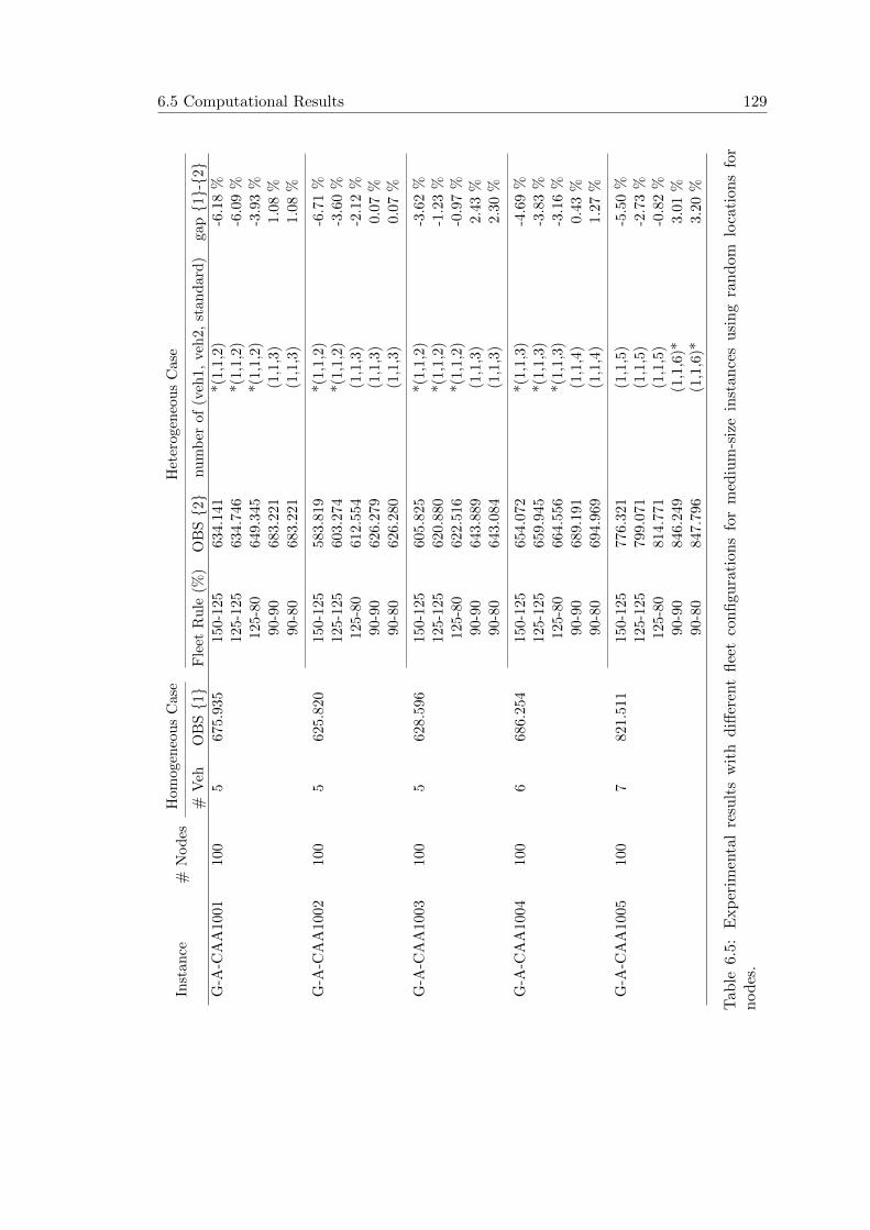
6.5 Computational Results 129
Inst
ance
#N
odes
Hom
ogen
eous
Cas
eH
eter
ogen
eous
Case
#V
ehO
BS{1}
Fle
etR
ule
(%)
OB
S{2}
num
ber
of
(veh
1,
veh2,
standard
)gap{1}-{2}
G-A
-CA
A10
0110
05
675.
935
150-
125
634.
141
*(1
,1,2
)-6
.18
%12
5-12
563
4.74
6*(1
,1,2
)-6
.09
%12
5-80
649.
345
*(1
,1,2
)-3
.93
%90
-90
683.
221
(1,1
,3)
1.0
8%
90-8
068
3.22
1(1
,1,3
)1.0
8%
G-A
-CA
A10
0210
05
625.
820
150-
125
583.
819
*(1
,1,2
)-6
.71
%12
5-12
560
3.27
4*(1
,1,2
)-3
.60
%12
5-80
612.
554
(1,1
,3)
-2.1
2%
90-9
062
6.27
9(1
,1,3
)0.0
7%
90-8
062
6.28
0(1
,1,3
)0.0
7%
G-A
-CA
A10
0310
05
628.
596
150-
125
605.
825
*(1
,1,2
)-3
.62
%12
5-12
562
0.88
0*(1
,1,2
)-1
.23
%12
5-80
622.
516
*(1
,1,2
)-0
.97
%90
-90
643.
889
(1,1
,3)
2.4
3%
90-8
064
3.08
4(1
,1,3
)2.3
0%
G-A
-CA
A10
0410
06
686.
254
150-
125
654.
072
*(1
,1,3
)-4
.69
%12
5-12
565
9.94
5*(1
,1,3
)-3
.83
%12
5-80
664.
556
*(1
,1,3
)-3
.16
%90
-90
689.
191
(1,1
,4)
0.4
3%
90-8
069
4.96
9(1
,1,4
)1.2
7%
G-A
-CA
A10
0510
07
821.
511
150-
125
776.
321
(1,1
,5)
-5.5
0%
125-
125
799.
071
(1,1
,5)
-2.7
3%
125-
8081
4.77
1(1
,1,5
)-0
.82
%90
-90
846.
249
(1,1
,6)*
3.0
1%
90-8
084
7.79
6(1
,1,6
)*3.2
0%
Tab
le6.
5:E
xp
erim
enta
lre
sult
sw
ith
diff
eren
tfl
eet
confi
gura
tion
sfo
rm
ediu
m-s
ize
inst
an
ces
usi
ng
ran
dom
loca
tion
sfo
rn
od
es.

130 Asymmetric and Heterogeneous Vehicle Routing Problem
Inst
ance
#N
odes
Hom
ogen
eous
Cas
eH
eter
ogen
eous
Cas
e
#V
ehO
BS{1}
Fle
etR
ule
(%)
OB
S{2}
num
ber
of(v
eh1,
veh2,
stan
dar
d)
gap{1}-{2}
G-C
-CA
A10
01
100
560
0.34
415
0-12
558
5.12
1*(
1,1,
2)-2
.54
%12
5-12
558
6.22
1*(
1,1,
2)-2
.35
%12
5-80
588.
736
*(1,
1,2)
-1.9
3%
90-9
060
4.69
6(1
,1,3
)0.
72%
90-8
060
4.24
4(1
,1,3
)0.
65%
G-C
-CA
A10
02
100
558
5.03
115
0-12
556
2.80
6*(
1,1,
2)-3
.80
%12
5-12
556
2.65
6*(
1,1,
2)-3
.82
%12
5-80
579.
052
(1,1
,3)
-1.0
2%
90-9
058
8.20
0(1
,1,3
)0.
54%
90-8
058
7.20
4(1
,1,3
)0.
37%
G-C
-CA
A10
03
100
556
6.00
515
0-12
554
3.78
4*(
1,1,
2)-3
.93
%12
5-12
554
9.95
8*(
1,1,
2)-2
.84
%12
5-80
552.
630
*(1,
1,2)
-2.3
6%
90-9
056
5.01
2(1
,1,3
)-0
.18
%90
-80
567.
901
(1,1
,3)
0.33
%
G-C
-CA
A10
04
100
666
5.51
115
0-12
563
3.02
6*(
1,1,
3)-4
.88
%12
5-12
563
5.76
1*(
1,1,
3)-4
.47
%12
5-80
647.
009
*(1,
1,3)
-2.7
8%
90-9
066
7.83
1(1
,1,4
)0.
35%
90-8
067
2.16
8(1
,1,4
)1.
00%
G-C
-CA
A10
05
100
765
2.42
415
0-12
563
5.24
8(1
,1,5
)-2
.63
%12
5-12
564
0.44
0(1
,1,5
)-1
.84
%12
5-80
648.
603
(1,1
,5)
-0.5
9%
90-9
066
8.15
6(1
,1,6
)*2.
41%
90-8
067
2.15
0(1
,1,6
)*3.
02%
Tab
le6.
6:E
xp
erim
enta
lre
sult
sw
ith
diff
eren
tfl
eet
con
figu
rati
ons
for
med
ium
-siz
ein
stan
ces
usi
ng
gri
dlo
cati
on
sfo
rn
od
es.

6.5 Computational Results 131
Thus, 120 different instances were considered in total. For each of them, 10 randomseeds (10 replicas) and an elapsed time of 1 minute were used.
The algorithm described in this chapter has been implemented as a Java application.An Intel QuadCore i5 at 3.2 GHz and 4 GB RAM was used to perform all tests, whichwere run over Windows XP.
Tables 6.3, 6.4, 6.5 and 6.6 contain, for each base instance, the following information:name of instance; number of nodes; number of vehicles; our best solution found for thehomogeneous case, OBS {1}; different fleet rules for the heterogeneous case, each ofthem defining a new routing instance; our best solution found for the heterogeneous case,OBS {3}; the obtained number of vehicles for the fleet configuration; and percentage gapbetween the BKS for the homogeneous case and the OBS for the heterogeneous case.Instances are distributed in the tables according to their sizes (50 or 100 nodes) and thelocation of the nodes on territory (random or grid).
Observe that * highlights different number of vehicles. For example, on table 6.3,(1,1,1)* of the fifth row remarks that this heterogeneous solution is using one more vehiclethan the homogeneous solution. It uses one vehicle of 90% of capacity, one vehicle of80% and one ‘standard’ vehicle. Instead, *(1,1,0) of the sixth row remarks that thissolution is using one less ‘standard’ vehicle.
Figure 6.7: Surface Plot of Average Gap vs. Fleet Configuration
Figure 6.7 shows a 3D scatter plot representing the average gap associated with eachof the 6 fleet configurations considered in this article. In other words, for each fleet rule,the twenty gaps with respect to the homogeneous OBS –one per base instance– havebeen averaged. From these results, it can be noticed the following:
• Just by employing two large vehicles (fleet 150-125) instead of two ‘standard’ ve-

132 Asymmetric and Heterogeneous Vehicle Routing Problem
hicles (fleet 100-100), it is possible to obtain noticeable costs reductions that cango up to 10% in some instances (e.g., G-A-CAA0502).
• Likewise, when using two small vehicles (fleet 90-80) instead of two ‘standard’vehicles, costs can suffer an increase of about 5% for some instances (e.g., G-C-CAA0504).
Therefore, it can be concluded that routing costs can be in fact quite sensitive tosmall variations in the fleet configuration. This justifies the necessity for employing newapproaches in real-life routing applications, i.e., algorithms which are able to deal withboth asymmetric costs as well as heterogeneous fleets.
6.6 Conclusions
In this chapter, we have discussed the importance of taking into account heterogeneousfleets in realistic Vehicle Routing Problems. Despite the fact that most real-life fleetsof vehicles are heterogeneous and that real-life distances are frequently asymmetric –especially in urban transportation–, there is a lack of works considering both situationssimultaneously. Accordingly, we have presented a multi-start process for solving theAsymmetric Heterogeneous Vehicle Routing Problem. This algorithm combines a ran-domized savings algorithm (SR-GCWS-CS) with three local search processes specificallyadapted to the heterogeneity of fleets in real-life scenarios.
A set of benchmarks for the AHVRP have been developed and a sensitivity analysison the fleet composition has been performed. This experiment shows how decision-makers can benefit from our approach when deciding the actual composition of theirheterogeneous fleets.

Contributions
Main contributions
The thesis has been introduced hybrid methodologies that integrates several techniquesto efficiently tackle six combinatorial problems related to road transport. It starts withtheoretical problems and evolves into more realistic scenarios, a study of different variantsfocusing on the impact that causes the asymmetry of the costs and the heterogeneity ofthe fleet has been presented, and a real problem of Home Health Care service in the cityof Ferrara, Italy, has been solved. Below detailed contributions are presented for eachchapter.
Our proposed Tailored Lagrangian Metaheuristic (TLM) method has been presentedin Chapter 1, this metaheuristic method is based on the Lagrangian Relaxation tech-nique. This scheme has been used to tackle the Traveling Salesman Problem (TSP),showing very good results both in terms of the quality of the solution and in terms ofcomputational efficiency.
Our proposed TLM method uses the Subgradient algorithm combined with a heuris-tic. The motivation of our method is the common sense belief that dual solutions mustobviously be relevant to primal solutions. The new introduced parameter has improvedsignificantly algorithm’s convergence on the optimal solution.
Our proposed TLM has been included into a Variable Neighborhood Search frame-work to tackle the Capacitated Vehicle Routing Problem (CVRP), in Chapter 2.
The presented hybrid methodology combines a randomized version of the Clarke andWright Savings heuristic with Constraint Programming and our Tailored LagrangianMetaheuristic to efficiently solve CVRP instances. These techniques have been embeddedinto a Multi-Start Variable Neighborhood Descent framework. According to the testsperformed, the proposed algorithm is competitive with state-of-the-art metaheuristics.
Our proposed TLM has been used to calculate routing cost for each vehicle sepa-rately. It solves all routes in negligible times and is an efficient alternative for intra-routeoptimization processes and avoids defining intra-route moves. Moreover, it ensures thepartial optimality of most solutions from the routing perspective. The reason is that,since we are considering a relatively small number of customers per route, the proposedapproach can quickly find the optimal solution to most TSP instances.
Chapter 3 presents a real-life application of constraint solving technologies to theHome Health Care problem for the city of Ferrara, Italy. Our proposed Tailored La-
133

134 Contributions
grangian Metaheuristic has been included into a Constraint Programming frameworkusing a search algorithm based on Large Neighborhood Search.
Our proposed TLM has been used to calculate traveling time for each nurse sepa-rately. It has been compared respect ASP and Comet technologies, obtaining that ourproposed TLM was the fastest, it ensures the partial optimality of most solutions fromthe routing perspective. The reason is that, since there are a relatively small number ofpatients per nurse, the proposed approach can quickly find the optimal solution to mostTSP instances.
An adaptation of our TLM for the Asymmetric Traveling Salesman Problem (ATSP)is presented in Chapter 4. For this problem, the out-degree constraints are relaxed andEdmond’s Algorithm is used to solve the dual problem. In this metaheuristic approach,a new heuristic to obtain a feasible solution from a dual one is proposed.
The results have shown that the new parameter has improved significantly Subgra-dient’s convergence on the optimal solution and it is showing good results in termsof the quality of the results. However, it is not showing a good behavior in terms ofcomputational efficiency.
A hybrid algorithm for solving the Asymmetric Capacitated Vehicle Routing Prob-lem (ACVRP) has been presented in Chapter 5. The proposed algorithm is based onthe randomized Clarke and Wright Savings algorithm (SR-GCWS), combined with twolocal search processes specifically adapted to the asymmetric nature of costs in real-lifescenarios.
The results show that our approach is able to produce competitive results for theACVRP while, at the same time, it is much simpler to implement and requires lessparameters –and fine-tuning efforts– than current state-of-the-art algorithms.
In Chapter 6, the proposed asymmetric adaptation of the SR-GCWS algorithm,presented in Chapter 5, has been modified to tackle the Asymmetric HeterogeneousVehicle Routing Problem (AHVRP). Our approach combines the SR-GCWS, developedby Juan et al. (2010) for the CVRP, with the modified Clarke and Wright Savingsheuristic, presented by Prins (2002) for the HVRP.
A set of benchmarks for the AHVRP have been developed and a sensitivity analysison the fleet composition has been performed. This experiment shows how decisionmakers can benefit from our approach when deciding the actual composition of theirheterogeneous fleets.
Finally, the hybrid VNS methodology described in Chapter 2 has been registeredwith the following software license:
• D. Guimarans, R. Herrero, J.J. Ramos, and M.A. Piera. ITSLogisim SimulationSuite 1.0 and ITSLogiSim Optimization Suite 1.0. Registered at Universitat Aut-noma de Barcelona, 30th June 2010.
Currently, the company Digital Aeronautics Engineering Services is using this soft-ware license under a commercial agreement. Combined with a clustering algorithm, itis being applied to solve problems up to 22,000 customers and more than 5,000 plannedroutes.

Contributions 135
Conclusions
The conclusions of this thesis can be summarized as follows:
• The Tailored Lagrangian Metaheuristic has been developed to tackle the TravelingSalesman Problem, it is based on the Lagrangian Relaxation.
• This metaheuristic is competitive in terms of both results and computational ef-ficiency for the symmetric scenarios. However, the impact of the asymmetry ofthe cost in our metaheuristic has been studied, its adaptation for the asymmetricscenarios is only showing good results in terms of quality, but it is not showing agood behavior in terms of computational efficiency.
• Our proposed metaheuristic has been integrated into a hybrid methodology com-bine with Constraint Programming to tackle the Capacitated Vehicle RoutingProblem. Our metaheuristic solves optimally all routes in negligible times.
• An application using our metaheuristic has been developed for a real scenario, theHome Health Care service in Ferrara, Italy. Our proposed metaheuristic, whichsolves optimally all routes consuming 10% of the computation time, has beenincluded into a Constraint Programming framework using a search algorithm basedon Large Neighborhood Search.
• The impact of the asymmetry of the cost has been studied tackling the Asymmetricversion of the Capacitated Vehicle Routing Problem. The randomized Clarke andWright Savings algorithm has been adapted combined with two local search pro-cesses specifically designed for the asymmetric nature of costs in real-life scenarios.Unlike other approaches, this adaptation has been flexible and it is competitivewith state-of-the-art metaheuristics.
• This Clarke and Wright approach has been adapted to consider Heterogeneousfleets. A study of the impact that causes the heterogeneity of the fleet has beenpresented showing that different fleet configurations can need one more or lessvehicle than the homogeneous solution, and the total cost can be reduced up to10% or increase up to 5% for different fleet configurations.
Future Research
As it can be appreciated in Chapter 4, the proposed dual problem for the ATSP hasnot been able to produce results quickly, in part derived from the running time ofEdmonds’ algorithm. In fact, the research of the scientific community is more focusedon the Lagrangian Relaxation for the ATSP based on the Assignment Problem. Adaptour Tailored Lagrangian Metaheuristic to this relaxation could be quite interesting todevelop as future work.

136 Contributions
Furthermore, it can be developed a parallel implementation of the algorithm pre-sented in Chapter 5–6, aiming to significantly accelerate its execution speed when deal-ing with large-scale instances. In this context, the splitting process can be designed torun different splitting policies in a parallel computing environment sharing a centralizedhash table among all threads. In addition, the entire multi-start process can be designedto run in a parallel computing environment using several distributed hash tables whichcommunicate among themselves to share information at certain time periods.
As for future work, the following lines of research are suggested to adapt the SR-GCWS-CS to solve some variants of VRP:
• VRP with Time Windows Each customer is associated with a time intervaland can only be served within this interval. When the next edge is selected fromsavingList, it must be verified whether the customer is served within its timeinterval before merging routes. It would be appropriate to use the well-knownInsertion heuristic during the local search process.
• Multi-Depot VRP It integrates a combinatorial assignment problem -which cus-tomers are to be assigned to each depot- with the several CVRPs that must besolved for each customers-depot assignment, this problem is less studied variant inthe literature. Before starting the current SR-GCWS-CS algorithm, each customercould be randomly assigned to a depot according to a distance-based criterion.Thus, each VRP could be solved independently using the SR-GWS algorithm, itcould be implemented in parallel using independent hash tables and without con-sidering the splitting process. Then, a new splitting-based local search could beapplied to all VRPs.
• Pickup-and-delivery VRP Each customer is associated by two quantities, rep-resenting one demand to be delivered at the customer and another demand to bepicked up and returned to the depot. When the next edge is selected from thesaving list, it must be verified whether both quantities can be satisfied while thetotal pickup and total delivery on the merged route are not exceeding the vehiclecapacity.
• Green VRP This variant deals with the optimization of energy consumption oftransportation which may clash with the designated economic objectives. It takesinto account the vehicles fuel tank capacity limitation and chooses the optimalplacement of Alternative Fueling Stations visits within the tour. When the nextedge is selected from the saving list, it must be verified the fuel tank capacity, if itis necessary to visit a fuel station, the routes will not merged. However, the costof the edge could be modified in the saving list adding the cost of inserting thenearest fuel station to the resultant route.
• Fuel Consumption Rate VRP New objective function is considered in whichthe cost function is a product of the total load (including the weight of the emptyvehicle) and the distance traveled minimizing fuel consumption. For this problem,

Contributions 137
the saving list should be reordered, it would be rather select the edge of maximumsaving related to the least loaded vehicles.
Publications
The work presented in this thesis has been partially published in the following journalarticles:
• Rosa Herrero, Alejandro Rodrıguez, Jose Caceres-Cruz, and Angel Juan (2014):Solving vehicle routing problems with asymmetric costs and heterogeneous fleets.International Journal of Advanced Operations Management, vol. 6(1), pp. 58-80.Inderscience Enterprises Ltd. DOI: 10.1504/IJAOM.2014.059620.
• Massimiliano Cattafi, Rosa Herrero, Marco Gavanelli, Maddalena Nonato, andFederico Malucelli (2015): An Application of Constraint Solving for Home HealthCare. AI Communications, vol. 28(2), pp. 215-237, indexed in IOS Press (IF 2015:0.547) ISSN: 0921-7126.
• Daniel Guimarans, Rosa Herrero, Daniel Riera, Angel Juan, and Juan Jose Ramos(2011): Combining probabilistic algorithms, Constraint Programming and La-grangian Relaxation to solve the Vehicle Routing Problem. Annals of Mathematicsand Artificial Intelligence, vol. 62(3), pp. 299-315, indexed in ISI SCI (FI = 0.358,4Q). ISSN: 1012-2443. DOI: 10.1007/s10472-011-9261-y.
• Daniel Guimarans, Rosa Herrero, Juan Jose Ramos, and Silvia Padron (2011):Solving Vehicle Routing Problems Using Constraint Programming and LagrangianRelaxation in a Metaheuristics Framework. International Journal of Informa-tion Systems and Supply Chain Management (IJISSCM), Special Issue: HybridAlgorithms for Solving Realistic Routing, Scheduling and Availability Problems,vol. 4(2), pp. 61-81. ISSN: 1935-5726. DOI: 10.4018/jisscm.2011040104.
Some parts of this work have also been presented in several international conferencesand published in the following related articles:
• Rosa Herrero, Juan Jose Ramos, and Daniel Guimarans (2009): Solving the Trav-elling Salesman Problem with Time Windows by Lagrangian Relaxation. In pro-ceeding of 21st European Modelling and Simulation Symposium (EMSS). Tenerife,Spain. September, 2009.
• Rosa Herrero, Juan Jose Ramos, and Daniel Guimarans (2010): Lagrangian Meta-heuristic for the Travelling Salesman Problem. In proceedings of Operational Re-search Annual Conference (OR 52). Surrey, UK. September, 2010.
• Rosa Herrero, Daniel Guimarans, Juan Jose Ramos, and Silvia Padron (2010):A Variable Neighbourhood Search Combining Constraint Programming and La-grangian Relaxation for Solving Routing Problems. In proceedings of 2010 Sum-mer Computer Simulation Conference (SCSC’10). Ottawa, Canada. July, 2010.

138 Contributions
• Daniel Guimarans, Rosa Herrero, Daniel Riera, Angel Juan, and Juan Jose Ramos(2010): Combining Constraint Programming, Lagrangian Relaxation and Proba-bilistic Algorithms to solve the Vehicle Routing Problem. In proceedings of 17thInternational RCRA workshop (RCRA 2010): Experimental Evaluation of Algo-rithms for Solving Problems with Combinatorial Explosion. Bologna, Italy. June,2010. ISBN: 1613-0073. http://ceur-ws.org/Vol-616/paper04.pdf
• Massimiliano Cattafi, Rosa Herrero, Marco Gavanelli, Maddalena Nonato, FedericoMalucelli, and Juan-Jose Ramos (2012): Improving quality and efficiency in homehealth care: an application of constraint logic programming for the Ferrara NHSunit. In Agostino Dovier and Vıtor Santos Costa, editors, Technical Communica-tions of the 28th International Conference on Logic Programming (ICLP’12), vol-ume 17 of Leibniz International Proceedings in Informatics (LIPICS), pp. 415-424,Dagstuhl, Germany, 2012. ISSN: 1868-8969. DOI: 10.4230/LIPIcs.ICLP.2012.415
• Massimiliano Cattafi, Rosa Herrero, Marco Gavanelli, Maddalena Nonato, FedericoMalucelli and Juan Jose Ramos (2012): An Application of Constraint Solvingfor Home Health Care. In proceedings of 19th RCRA workshop on ExperimentalEvaluation of Algorithms for Solving Problems with Combinatorial Explosion. Inassociation with the 12-th AI*IA Symposium on Artificial Intelligence. Rome,Italy, 14-15 June 2012.
• Jose Caceres-Cruz, Daniel Riera, Roman Buil, Angel Juan, and Rosa Herrero(2013): Multi-start Approach for Solving an Asymmetric Heterogeneous VehicleRouting Problem in a Real Urban Context. In proceedings of 2nd InternationalConference on Operations Research and Enterprise Systems (INSTICC-ICORES)February, 2013.
Copy of scientific publications, references and any other additional information willbe provided upon request (Email: [email protected]).

References
Alba, E. (2005). Parallel metaheuristics: a new class of algorithms (Vol. 47). JohnWiley & Sons.
Alba, E., Blum, C., Asasi, P., Leon, C., & Gomez, J. A. (2009). Optimization techniquesfor solving complex problems (Vol. 76). John Wiley & Sons.
Alba, E., & Dorronsoro, B. (2008). A hybrid cellular genetic algorithm for the ca-pacitated vehicle routing problem. In A. Abraham, C. Grosan, & W. Pedrycz(Eds.), Engineering Evolutionary Intelligent Systems (Studies in ComputationalIntelligence, 82) (pp. 379–422). Springer Berlin Heidelberg.
Alba, E., Luque, G., & Nesmachnow, S. (2013). Parallel metaheuristics: recent advancesand new trends. International Transactions in Operational Research, 20 (1), 1–48.
Altinel, I., & Oncan, T. (2005). A new enhancement of the Clarke and Wright savingsheuristic for the capacitated vehicle routing problem. Journal of the OperationalResearch Society , 56 , 954–961.
Andziulis, A., Dzemydiene, D., Steponavicius, R., & Jakovlev, S. (2011). Compar-ison of two heuristic approaches for solving the production scheduling problem.Information Technology And Control , 40 (2), 118–122.
Applegate, D., Archer, A., Gopalakrishnan, V., Lee, S., & Ramakrishnan, K. K. (2010).Optimal Content Placement for a Large-scale VoD System. In Proceedings of the6th International Conference Co-NEXT ’10 (pp. 4:1–12). ACM.
Applegate, D., Bixby, R., Chvatal, V., & Cook, W. (2006). The Traveling SalesmanProblem: A Computational Study. Princeton University Press.
Applegate, D., Bixby, R., Chvatal, V., & Cook, W. (2015, August). Concorde. Retrievedfrom www.tsp.gatech.edu
Apt, K., & Wallace, M. (2007). Constraint Logic Programming using ECLiPSe. Cam-bridge University Press.
Asadpour, A., Goemans, M. X., Madry, A., Gharan, S. O., & Saberi, A. (2010). AnO(log n/log log n)-approximation algorithm for the asymmetric traveling salesmanproblem.
Ascheuer, N., Fischetti, M., & Grotschel, M. (2001). Solving the asymmetric travellingsalesman problem with time windows by branch-and-cut. Mathematical Program-ming , 90 (3), 475–506.
Ascheuer, N., Junger, M., & Reinelt, G. (2000). A branch & cut algorithm for the asym-metric traveling salesman problem with precedence constraints. Computational
139

140 References
Optimization and Applications, 17 (1), 61–84.
Bai, J., Zhu, J., Yang, G.-K., & Pan, C.-C. (2011). Collaborative optimization undera control framework for ATSP. In Y. Tan, Y. Shi, Y. Chai, & G. Wang (Eds.),Advances in Swarm Intelligence (pp. 355–363). Springer.
Balas, E., & Christofides, N. (1981). A restricted Lagrangean approach to the travelingsalesman problem. Mathematical Programming , 21 (1), 19–46.
Balas, E., & Toth, P. (1985). Branch and Bound Methods. In E. Lawler, J. Lenstra,A. R. Kan, & D. Shmoys (Eds.), The Traveling Salesman Problem (pp. 361–401).John Wiley & Sons, Chichester.
Baldacci, R., Battarra, M., & Vigo, D. (2008). Routing a Heterogeneous Fleet of Vehicles.In B. Golden, S. Raghavan, & E. Wasil (Eds.), The vehicle routing problem: Latestadvances and new challenges (Vol. 43, pp. 3–27). Springer US.
Baldacci, R., & Mingozzi, A. (2009). A unified exact method for solving different classesof vehicle routing problems. Mathematical Programming , 120 (2), 347–380.
Baldacci, R., Toth, P., & Vigo, D. (2010). Exact algorithms for routing problems undervehicle capacity constraints. Annals of Operations Research, 175 , 213–245.
Barahona, F., & Anbil, R. (2000). The Volume Algorithm: producing primal solutionswith a subgradient method. Mathematical Programming , 87 (3), 385–399.
Basart, J. (2003). Grafs: fonaments i algorismes (Third ed.). Universitat Autonoma deBarcelona.
Begur, S. V., Miller, D. M., & Weaver, J. R. (1997). An integrated spatial DSS forscheduling and routing home-health care nurses. Interfaces, 27 (4), 35–48.
Beldiceanu, N., Carlsson, M., & Rampon, J.-X. (2005). Global Constraint Catalog(Vol. 8; Tech. Rep. No. 2005). Kista, Sweden: Swedish Institute of Computer Sci-ence (SICS). Retrieved from http://eprints.sics.se/2366/01/SICS-T--2005
-08--SE.pdf
Beldiceanu, N., & Contejean, E. (1994). Introducing global constraints in CHIP. Math-ematical and Computer Modelling , 20 (12), 97–123.
Bell, J., & McMullen, P. (2004). Ant Colony Optimization Techniques For The VehicleRouting Problem. Advanced Engineering Informatics(18), 41–48.
Bellman, R. (1962). Dynamic Programming Treatment of the Travelling SalesmanProblem. Journal of the ACM , 9 (1), 61–63.
Belloni, A., & Lucena, A. (2000). A relax and cut algorithm for the traveling salesmanproblem. In 17th international symposium on mathematical programming.
Bent, R., & Van Hentenryck, P. (2004). A two-stage hybrid local search for the vehiclerouting problem with time windows. Transportation Science, 38 (4), 515–530.
Berger, J., & Barkaoui, M. (2003). A Hybrid Genetic Algorithm for the CapacitatedVehicle Routing Problem. In Proceedings of the International Genetic and Evolu-tionary Computation Conference –GECCO 2003 (pp. 646–656). Illinois, Chicago,USA: Springer-Verlag.
Bertels, S., & Fahle, T. (2006). A hybrid setup for a hybrid scenario: combiningheuristics for the home health care problem. Computers & Operations Research,33 (10), 2866–2890.
References 141
Bertsekas, D. P. (1999). Nonlinear Programming. Belmont, Massachusetts: AthenaScientific.
Bessiere, C. (2006). Constraint propagation. In F. Rossi, P. van Beek, & T. Walsh(Eds.), Handbook of constraint programming (pp. 29–83). Elsevier.
Bessiere, C., Hebrard, E., Hnich, B., zıltan, Z. K., & Walsh, T. (2006). FilteringAlgorithms for the NValue Constraint. Constraints, 11 (4), 271–293.
Bessiere, C., Katsirelos, G., Narodytska, N., Quimper, C.-G., & Walsh, T. (2010).Decomposition of the NValue Constraint. In Principles and Practice of ConstraintProgramming –CP 2010 (pp. 114–128).
Bolduc, M. C., Renaud, J., & Montreuil, B. (2006, June). Synchronized routing ofseasonal products through a production/distribution network. Central EuropeanJournal of Operations Research, 14 (2), 209–228.
Bontoux, B., Artigues, C., & Feillet, D. (2010). A memetic algorithm with a largeneighborhood crossover operator for the generalized traveling salesman problem.Computers and Operations Research, 37 (11), 1844–1852.
Borsani, V., Matta, A., Beschi, G., & Sommaruga, F. (2006). A home care schedulingmodel for human resources. In International Conference on Service Systems andService Management (Vol. 1, pp. 449–454). IEEE.
Boschetti, M., & Maniezzo, V. (2009). Benders decomposition, Lagrangean relaxationand metaheuristic design. Journal of Heuristics, 15 (3), 283–312.
Boyer, C. B. (1985). A history of mathematics (P. Press, Ed.). Princeton Univ.
Brandao, J. (2009). A deterministic tabu search algorithm for the fleet size and mixvehicle routing problem. European Journal of Operational Research, 195 (3), 716–728.
Brandao, J. (2011). A tabu search algorithm for the heterogeneous fixed fleet vehiclerouting problem. Computers & Operations Research, 38 (1), 140–151.
Braysy, O. (2003). A reactive variable neighborhood search for the vehicle-routingproblem with time windows. INFORMS Journal on Computing , 15 (4), 347–368.
Brewka, G., Eiter, T., & Truszczynski, M. (2011). Answer set programming at a glance.Communications of the ACM , 54 (12), 92–103.
Buriol, L., Franca, P. M., & Moscato, P. (2004). A new memetic algorithm for theasymmetric traveling salesman problem. Journal of Heuristics, 10 (5), 483–506.
Burke, E. K., Cowling, P. I., & Keuthen, R. (2001). Effective local and guided variableneighbourhood search methods for the asymmetric travelling salesman problem. InApplications of evolutionary computing (pp. 203–212). Springer Berlin Heidelberg.
Buxey, G. (1979). The Vehicle Scheduling Problem and Monte Carlo Simulation. Journalof Operational Research Society , 30 , 563–573.
Caprara, A., Fischetti, M., & Toth, P. (1996). A heuristic algorithm for the set coveringproblem. In Integer Programming and Combinatorial Optimization (pp. 72–84).Springer.
Caprara, A., Fischetti, M., & Toth, P. (2002). Modeling and Solving the TrainTimetabling Problem. Operations Research, 50 (5), 851–861.
Caprara, A., Toth, P., & Fischetti, M. (2000). Algorithms for the set covering problem.

142 References
Annals of Operations Research, 98 (1), 353–371.
Carpaneto, G., Dell’Amico, M., & Toth, P. (1995). Exact solution of large-scale, asym-metric traveling salesman problems. ACM Transactions on Mathematical Software(TOMS), 21 (4), 394–409.
Carpaneto, G., & Toth, P. (1980). Some new branching and bounding criteria for theasymmetric travelling salesman problem. Management Science, 26 (7), 736–743.
Carrabs, F., Cordeau, J.-F., & Laporte, G. (2007). Variable neighborhood search forthe pickup and delivery traveling salesman problem with lifo loading. INFORMSJournal on Computing , 19 (4), 618–632.
Caseau, Y., & Laburthe, F. (1997, Jul.). Solving small TSPs with constraints. InL. Naish (Ed.), Proc. of the 14th international conference on logic programming(pp. 316–330). The MIT Press.
Cattafi, M., Herrero, R., Gavanelli, M., Nonato, M., & Malucelli, F. (2012). ImprovingQuality and Efficiency in Home Health Care: an application of Constraint LogicProgramming for the Ferrara NHS unit. In Iclp (technical communications) (pp.415–424).
Cattafi, M., Herrero, R., Gavanelli, M., Nonato, M., & Malucelli, F. (2015). An Appli-cation of Constraint Solving for Home Health Care. AI Communications, 28 (2),215–237.
Celik, Y., & Ulker, E. (2012). A marriage in honey bee optimisation approach to asym-metric traveling salesman problem. International Journal of Innovative Comput-ing, Information and Control , 8 (6), 4123–4132.
Chen, M. (1996). A mathematical programming model for AGVs planning and controlin manufacturing systems. Computers & industrial engineering , 30 (4), 647–658.
Chen, S. M., & Chien, C. Y. (2011). Solving the traveling salesman problem based on thegenetic simulated annealing ant colony system with particle swarm optimizationtechniques. Expert Systems with Applications, 38 (12), 14439–14450.
Cheng, E., & Rich, J. L. (1998). A home health care routing and scheduling problem(Tech. Rep. Nos. CAAM TR98–04). Rice University.
Cheng, R., & Gen, M. (1994). Crossover on intensive search and traveling salesmanproblem. Computers & Industrial Engineering , 27 (1), 485–488.
Choi, E., & Tcha, D. W. (2007). A column generation approach to the heterogeneousfleet vehicle routing problem. Computers & Operations Research, 34 (7), 2080–2095.
Choi, I. C., Kim, S. I., & Kim, H. S. (2003). A genetic algorithm with a mixed regionsearch for the asymmetric traveling salesman problem. Computers & OperationsResearch, 30 (5), 773–786.
Christofides, N. (1976). Worst-case analysis of a new heuristic for the travelling salesmanproblem (Tech. Rep. No. RR-388). Carnegie-Mellon Univ Pittsburgh Pa Manage-ment Sciences Research Group.
Christofides, N., Mingozzi, A., & Toth, P. (1979). The vehicle routing problem. InN. Christofides et al. (Eds.), Combinatorial optimization (pp. 315–338). Wiley,Chichester, U.K..

References 143
Cipra, B. (1993). Quick trips. SIAM News, 26 .
Cirasella, J., Johnson, D. S., McGeoch, L. A., & Zhang, W. (2001). The asymmet-ric traveling salesman problem: Algorithms, instance generators, and tests. InA. L. Buchsbaum & J. Snoeyink (Eds.), Algorithm engineering and experimenta-tion (Vol. 2153, pp. 32–59). Springer.
Clarke, G., & Wright, J. (1964). Scheduling of Vehicles from a central Depot to aNumber of Delivering Points. Operations Research, 12 (4), 568–581.
Cordeau, J., & Laporte, G. (2004). Tabu search heuristics for the vehicle routingproblem. In C. Rego & B. Alidaee (Eds.), (pp. 145–163). Boston, MA, U.S.A.:Kluwer Academic.
Cordeau, J., Laporte, G., Savelsbergh, M., & Vigo, D. (2007). Vehicle routing. InC. Barnhart & G. Laporte (Eds.), Handbook in operations research and manage-ment science (Vol. 14, pp. 367–428). Amsterdam, The Netherlands: Elsevier.
Cormen, T., Leiserson, C., Rivest, R., & Stein, C. (2001). Section 23.2: The algorithmsof Kruskal and Prim. In M. Press & S. E. McGraw-Hill (Eds.), Introduction toalgorithms (pp. 567–574).
Crispim, J., & Brandao, J. (2001). Reactive tabu search and variable neighbourhooddescent applied to the vehicle routing problem with backhauls. In Mico2001 4thmetaheuristic international conference, porto, portugal.
Dantzig, G. B., Fulkerson, R., & Johnson, S. (1954). Solution of a large-scale TravelingSalesman Problem. Operations Research, 2 , 393–410.
Dantzig, G. B., & Ramser, J. H. (1959). The truck dispatching problem. ManagementScience, 6 , 80–91.
Dantzig, G. B., & Wolfe, P. (1960). Decomposition principle for linear programs. Oper-ations Research, 8 , 101–111.
De Franceschi, R., Fischetti, M., & Toth, P. (2006). A new ILP-based refinementheuristic for vehicle routing problems. Mathematical Programming , 105 (2-3), 471–499.
Deep, K., & Mebrahtu, H. (2011). Combined mutation operators of genetic algorithmfor the travelling salesman problem. International Journal of Combinatorial Op-timization Problems and Informatics, 2 (3), 1–23.
Delisle, P., Gravel, M., Krajecki, M., Gagne, C., & Price, W. L. (2005). A sharedmemory parallel implementation of ant colony optimization. In Proceedings of the6th metaheuristics international conference (pp. 257–264).
Delisle, P., Krajecki, M., & Gravel, M. (2009). Multi-colony parallel ant colony op-timization on SMP and multi-core computers. In 2009 world congress on na-ture&biologically inspired computing (nabic).
Desrosiers, J., Sauve, M., & Soumis, F. (1988). Lagrangean relaxation methods forsolving the minimum fleet size multiple travelling salesman problem with timewindows. Management Science, 34 , 1005–1022.
Dorigo, M., & Gambardella, L. (2014). Ant-Q: A reinforcement learning approach tothe traveling salesman problem. In Proceedings of ML-95, Twelfth Intern. Conf.on Machine Learning (pp. 252–260).

144 References
Dorigo, M., & Gambardella, L. M. (1997). Ant colony system: a cooperative learningapproach to the traveling salesman problem. Evolutionary Computation, IEEETransactions on, 1 (1), 53–66.
Dorronsoro, B., Arias, D., Luna, F., Nebro, A. J., & Alba, E. (2007). A grid-basedhybrid cellular genetic algorithm for very large scale instances of the cvrp. In Highperformance computing & simulation conference (hpcs) (pp. 759–765).
Drexl, M. (2012). Rich vehicle routing in theory and practice. Logistics Research, 5 (1-2),47–63.
Edmonds, J. (1967). Optimum Branchings. Journal of Research of the National Bureauof Standards B , 71 , 233–240.
Edmonds, J., & Johnson, E. L. (1973). Matching, Euler tours and the Chinese postman.Mathematical programming , 5 (1), 88–124.
Elbenani, B., Ferland, J., & Gascon, V. (2008). Mathematical programming approach forrouting home care nurses. In Industrial Engineering and Engineering Management,IEEM 2008. IEEE International Conference on (pp. 107–111).
Escobar, J. W., Linfati, R., Baldoquin, M. G., & Toth, P. (2014). A Granular VariableTabu Neighborhood Search for the capacitated location-routing problem. Trans-portation Research Part B: Methodological , 67 , 344–356.
Euchi, J., & Chabchoub, H. (2010). A hybrid tabu search to solve the heterogeneousfixed fleet vehicle routing problem. Logistics Research, 2 (1), 3–11.
Eveborn, P., Ronnqvist, M., Einarsdottir, H., Eklund, M., Liden, K., & Almroth, M.(2009). Operations Research Improves quality and efficiency in Home Care. Inter-faces, 39 (1), 18–34.
Faulin, J., Gilibert, M., Juan, A. A., Ruiz, R., & Vilajosana, X. (2008). SR-1: Asimulation-based algorithm for the capacitated vehicle routing problem. Proceed-ings of the 2008 Winter Simulation Conference.
Faulin, J., & Juan, A. A. (2008). The ALGACEA-1 Method for the Capacitated VehicleRouting Problem. International Transactions in Operational Research, 15 , 1–23.
Feo, T., & Resende, M. (1995). Greedy randomized adaptive search procedures. Journalof Global Optimization, 6 (2), 109–133.
Fernandez, P., Garcıa, L., Mayado, A., & Sanchıs, J. (2000). A Real Delivery ProblemDealt with Monte Carlo Techniques. TOP , 8 , 57–71.
Festa, P., & Resende, M. (2009). An Annotated Bibliography of GRASP–Part I: Algo-rithms. International Transactions in Operational Research, 16 , 1–24.
Fischetti, M., Lodi, A., & Toth, P. (2003). Solving real-world ATSP instances bybranch-and-cut. In Combinatorial optimization–eureka, you shrink! (pp. 64–77).Springer.
Fischetti, M., Lodi, A., & Toth, P. (2007). Exact methods for the asymmetric travelingsalesman problem. In The traveling salesman problem and its variations (pp. 169–205). Springer.
Fischetti, M., Salazar, J., & Toth, P. (1997a). A branch-and-cut algorithm for thesymmetric generalized Traveling Salesman Problem. Operations Research, 45 ,378–394.
References 145
Fischetti, M., & Toth, P. (1992). An additive bounding procedure for the asymmetrictravelling salesman problem. Mathematical Programming , 53 (1–3), 173–197.
Fischetti, M., & Toth, P. (1997b). A polyhedral approach to the asymmetric travelingsalesman problem. Management Science, 43 (11), 1520–1536.
Fischetti, M., Toth, P., & Vigo, D. (1994). A branch-and-bound algorithm for thecapacitated vehicle routing problem on directed graphs. Operations Research,42 (5), 846–859.
Fisher, M. L. (2004). The Lagrangian Relaxation Method for Solving Integer Program-ming Problems. Management Science, 50 (12S), 1861–1871.
Fisher, M. L., & Jaikumar, R. (1981). A generalized assignment heuristic for vehicle-routing. Networks, 11 (2), 109–124.
Fisher, M. L., Jornsten, K. O., & Madsen, O. B. G. (1997). Vehicle routing with timewindows: Two optimization algorithms. Operations research, 45 (3), 488–492.
Focacci, F., Lodi, A., & Milano, M. (2002). A hybrid exact algorithm for the TSPTW.INFORMS Journal on Computing , 14 (4), 403–417.
Freisleben, B., & Merz, P. (1996). New genetic local search operators for the travelingsalesman problem. In Parallel problem solving from nature–ppsn iv (pp. 890–899).Springer.
Fukunaga, A. S., & Korf, R. E. (2007). Bin completion algorithms for multicontainerpacking, knapsack, and covering problems. J. Artif. Int. Res., 28 (1), 393–429.
Garrido, P., Castro, C., & Monfroy, E. (2009). Towards a Flexible and AdaptableHyperheuristic Approach for VRPs. In Ic-ai (pp. 311–317).
Gaskell, T. (1967). Bases for the vehicle fleet scheduling. Operational Research Quarterly ,18 , 281–295.
Gavanelli, M. (2002). An Algorithm for Multi-Criteria Optimization in CSPs. In Ecai2002. proceedings of the 15th european conference on artificial intelligence (pp.136–140). IOS Press.
Gavish, B., & Pirkul, H. (1986). Computer and Database Location in DistributedComputer Systems. Computers, IEEE Transactions on Computers, 35 (7), 583–590.
Gebser, M., Kaminski, R., Kaufmann, B., Ostrowski, M., Schaub, T., & Schneider, M.(2011). Potassco: The Potsdam answer set solving collection. AI Communications,24 (2), 105–124.
Gen, M., & Cheng, R. (2000). Genetic algorithms and engineering optimization (Vol. 7).John Wiley & Sons.
Gendreau, M., Hertz, A., & Laporte, G. (1994). A Tabu Search Heuristic for the VehicleRouting Problem. Management Science, 40 , 1276–1290.
Gendreau, M., Laporte, G., Musaraganyi, C., & Taillard, E. (1999). A tabu searchheuristic for the heterogeneous fleet vehicle routing problem. Computers & Oper-ations Research, 26 (12), 1153–1173.
Gendron, B., Khuong, P.-V., & Semet, F. (2013). A lagrangian-based branch-and-bound algorithm for the two-level uncapacitated facility location problem with single-assignment constraints. Montreal: Cirrelt.

146 References
Geoffrion, A. (1974). Lagrangean relaxation for integer programming. In M. Balinski(Ed.), Approaches to integer programming (Vol. 2, pp. 82–114). Springer BerlinHeidelberg.
Germs, R., Goldengorin, B., & Turkensteen, M. (2012). Lower tolerance-based branchand bound algorithms for the ATSP. Computers & Operations Research, 39 (2),291–298.
Giuliani, M. V., Scopelliti, M., & Fornara, F. (2005). Elderly people at home: techno-logical help in everyday activities. In Robot and human interactive communication,2005. roman 2005. ieee international workshop on (pp. 365–370).
Glover, F. (1986). Future paths for integer programming and links to artificial intelli-gence. Computers & operations research, 13 (5), 533–549.
Glover, F., Gutin, G., Yeo, A., & Zverovich, A. (2001). Construction heuristics for theasymmetric TSP. European Journal of Operational Research, 129 (3), 555–568.
Glover, F., & Laguna, M. (1997). Tabu search. Kluwer Academic Publishers.
Glover, F., & Laguna, M. (2013). Tabu search (Second Edition ed.). Springer.
Golden, B., Assad, A., Levy, L., & Gheysens, F. (1984). The Fleet Size and Mix VehicleRouting Problem. Computers & Operations Research, 11 (1), 49–66.
Golden, B., Assad, A. A., & Wasil, E. A. (2002). Routing Vehicles in the Real World:Applications in the Solid Waste, Beverage, Food, Dairy and Newspaper Industries.In P. Toth & D. Vigo (Eds.), The vehicle routing problem (pp. 245–286). SIAMMonographs on Discrete Mathematics and Applications.
Golden, B., Raghavan, S., & Wasil, E. A. (2008). The Vehicle Routing Problem: LatestAdvances and New Challenges (Vol. 43). Springer.
Gomes, C. P., Selman, B., & Crato, N. (1997). Heavy-Tailed Distributions in Combina-torial Search. In Cp (pp. 121–135).
Grotschel, M., & Holland, O. (1991). Solution of large-scale symmetric travelling sales-man problems. Mathematical Programming , 51 (1-3), 141–202.
Guignard, M. (2003). Lagrangean Relaxation. Sociedad de Estadıstica e InvestigacionOperativa, Top, 11 (2), 151–228.
Guimarans, D. (2012). Hybrid algorithms for solving routing problems (PhD Thesis).Universitat Autonoma de Barcelona. Departament de Telecomunicacio i Enginyeriade Sistemes. Retrieved from http://hdl.handle.net/10803/96386
Guimarans, D., Herrero, R., Ramos, J., & Padron, S. (2011a). Solving vehicle routingproblems using constraint programming and lagrangean relaxation in a metaheuris-tics framework. International Journal of Information Systems and Supply ChainManagement .
Guimarans, D., Herrero, R., Ramos, J. J., & Padron, S. (2013). Management innovationsfor intelligent supply chains. In J. Wang (Ed.), (pp. 123–143). IGI Global.
Guimarans, D., Herrero, R., Riera, D., Juan, A., & Ramos, J. (2010). CombiningConstraint Programming, Lagrangian Relaxation and Probabilistic Algorithms toSolve the Vehicle Routing Problem. In Proceedings of the 17th rcra internationalworkshop. Bologna, Italy.
Guimarans, D., Herrero, R., Riera, D., Juan, A. A., & Ramos, J. J. (2011b). Combining

References 147
probabilistic algorithms, Constraint Programming and Lagrangian Relaxation tosolve the Vehicle Routing Problem. Annals of Mathematics and Artificial Intelli-gence, 62 (3-4), 299–315.
Gutin, G., & Karapetyan, D. (2010). A memetic algorithm for the generalized travelingsalesman problem. Natural Computing , 9 (1), 47–60.
Gutin, G., & Punnen, A. P. (2002). The Traveling Salesman Problem and Its Variations(Vol. 12). Springer Science & Business Media.
Hanada, K., & Hirayama, K. (2011). Distributed Lagrangian Relaxation Protocol forthe Over-constrained Generalized Mutual Assignment Problem. In D. Kinny, J.-j. Hsu, G. Governatori, & A. Ghose (Eds.), Agents in principle, agents in practice(Vol. 7047, pp. 174–186). Springer Berlin Heidelberg.
Hansen, K. H., & Krarup, J. (1974). Improvements of the Held–Karp algorithm for thesymmetric traveling-salesman problem. Mathematical Programming , 7 (1), 87–96.
Hansen, P., & Mladenovic, N. (2003). A tutorial on variable neighborhood search(Tech. Rep. No. G-2003-46). Montreal, Canada: Groupe d’Etudes et de Rechercheen Analyse des Decisions (GERAD). Retrieved from http://www.gerad.ca/
fichiers/cahiers/G-2003-46.pdf
Hansen, P., & Mladenovic, N. (2006). First vs. best improvement: An empirical study.Discrete Applied Mathematics, 154 (5), 802–817.
Haralick, R. M., & Elliott, G. L. (1980). Increasing Tree Search Efficiency for ConstraintSatisfaction Problems. Artif. Intell., 14 (3), 263–313.
Hartl, R., Hasle, G., & Janssens, G. (2006). Special issue on Rich Vehicle RoutingProblems. Central European Journal of Operations Research, 14 (2), 103–104.
Hasle, G., & Kloster, O. (2007). Industrial vehicle routing. In G. Hasle, K. Lie,& E. Quak (Eds.), Geometric modelling, numerical simulation, and optimization(pp. 397–435). Berlin, Germany: Springer-Verlag.
Hebrard, E., Marx, D., O’Sullivan, B., & Razgon, I. (2011). Soft Constraints of Differenceand Equality. J. Artif. Intell. Res. (JAIR), 41 , 97–130.
Held, M., & Karp, R. (1970). The Traveling Salesman Problem and Minium SpanningTrees. Operations Research, 18 , 1138–1162.
Held, M., & Karp, R. (1971). The Traveling Salesman Problem and Minium SpanningTrees: Part II. Mathematical Programming , 1 , 6–25.
Helsgaun, K. (2000). An effective implementation of the Lin–Kernighan traveling sales-man heuristic. European Journal of Operational Research, 126 (1), 106–130.
Helsgaun, K. (2009). General k-opt submoves for the Lin-Kernighan TSP heuristic.Mathematical Programming Computation, 1 (2-3), 119–163.
Herrero, R., Guimarans, D., Ramos, J. J., & Padron, S. (2010a). A variable neigh-bourhood search combining constraint programming and lagrangian relaxation forsolving routing problems. In Proceedings of the 2010 summer computer simulationconference (pp. 379–386).
Herrero, R., Ramos, J. J., & Guimarans, D. (2010b). Lagrangian Metaheuristic forthe Travelling Salesman Problem. In Extended abstracts of operational researchconference 52. Royal Holloway, University of London.

148 References
Herrero, R., Rodrıguez, A., Caceres-Cruz, J., & Juan, A. A. (2014). Solving vehiclerouting problems with asymmetric costs and heterogeneous fleets. InternationalJournal of Advanced Operations Management , 6 (1), 58–80.
Hiriart-Urruty, J., & Lemarechal, C. (1993). Convex Analysis and Minimization Algo-rithms (Vol. 1-2). Berlin, Germany: Springer Verlag.
Hoeft, J., & Palekar, U. (1997). Heuristics for the plate-cutting traveling salesmanproblem. IIE Transactions (Institute of Industrial Engineers), 29 (9), 719–731.
Hoffman, A., & Wolfe, P. (1985). The Traveling Salesman Problem. In E. Lawler,J. Lenstra, A. R. Kan, & D. Shmoys (Eds.), (pp. 1–16). John Wiley.
Hoffman, K. L., Padberg, M., & Rinaldi, G. (2013). Traveling Salesman Problem.In Encyclopedia of operations research and management science (pp. 1573–1578).Springer.
Holland, J. (1975). Adaptation in natural and artificial systems: an introductory anal-ysis with applications to biology, control, and artificial intelligence. Ann Arbor:University of Michigan Press.
Hooker, J. (2008). Integer Programming: Lagrangian Relaxation. In Encyclopedia ofOptimization (pp. 1667–1673). Springer.
Hulubei, T., & O’Sullivan, B. (2006). The Impact of Search Heuristics on Heavy-TailedBehaviour. Constraints, 11 (2-3), 159–178.
IBM ILOG CPLEX Optimization Studio. (2015). Retrieved from https://www.ibm
.com/developerworks/downloads/ws/ilogcplex/
Imran, A., Salhi, S., & Wassan, N. A. (2009). A variable neighborhood-based heuristic forthe heterogeneous fleet vehicle routing problem. European Journal of OperationalResearch, 197 (2), 509–518.
Irnich, S. (2008). A Unified Modeling and Solution Framework for Vehicle Routing andLocal Search-Based Metaheuristics. INFORMS Journal on Computing , 20 (2),270–287.
Jena, S. D., Cordeau, J.-F., & Gendron, B. (2014). Lagrangian Heuristics for Large-Scale Dynamic Facility Location with Generalized Modular Capacities. INFORMSJournal on Computing .
Jin Ai, T., & Kachitvichyanukul, V. (2009). Particle swarm optimization and two solu-tion representations for solving the capacitated vehicle routing problem. Computersand Industrial Engineering , 56 , 380–387.
Johnson, D., Gutin, G., McGeoch, L. A., Yeo, A., Zhang, W., & Zverovitch, A. (2007).Experimental analysis of heuristics for the ATSP. In The traveling salesman prob-lem and its variations (pp. 445–487). Springer.
Juan, A., Faulin, J., Jorba, J., Grasman, S., & Barrios, B. (2008). SR-2: A HybridIntelligent Algorithm for the Vehicle Routing Problem. In Proceedings of the 8thinternational conference on hybrid intelligent systems (pp. 78–83). Barcelona,Spain.
Juan, A., Faulın, J., Jorba, J., Riera, D., Masip, D., & Barrios, B. (2011). On the useof Monte Carlo simulation, cache and splitting techniques to improve the Clarkeand Wright savings heuristics. Journal of the Operational Research Society , 62 (6),

References 149
1085–1097.
Juan, A., Faulin, J., Ruiz, R., Barrios, B., & Caballe, S. (2010). The SR-GCWShybrid algorithm for solving the capacitated vehicle routing problem. Applied SoftComputing , 10 (1), 215–224.
Juan, A., Faulin, J., Ruiz, R., Barrios, B., Gilibert, M., & Vilajosana, X. (2009). Usingoriented random search to provide a set of alternative solutions to the capacitatedvehicle routing problem. Operations Research and Cyber-Infrastructure, 331–346.
Kallehauge, B., Larsen, J., & Madsen, O. B. (2006). Lagrangian duality applied to thevehicle routing problem with time windows. Computers & Operations Research,33 (5), 1464–1487.
Kanellakis, P.-C., & Papadimitriou, C. H. (1980). Local search for the asymmetrictraveling salesman problem. Operations Research, 28 (5), 1086–1099.
Karaboga, D., & Gorkemli, B. (2011). A combinatorial artificial bee colony algorithm fortraveling salesman problem. In Innovations in intelligent systems and applications(inista), 2011 international symposium on (pp. 50–53).
Karp, R. M. (1972). Reducibility among combinatorial problems. In R. Miller &J. Thatcher (Eds.), Complexity of computer computations (pp. 85–103). New York:Plenum Press.
Karp, R. M. (1979). A patching algorithm for the nonsymmetric traveling-salesmanproblem. SIAM Journal on Computing , 8 (4), 561–573.
Kautz, H., Horvitz, E., Ruan, Y., Gomes, C., & Selman, B. (2002). Dynamic RestartPolicies. In Aaai/iaai (p. 674-681).
Kaya, L. G., & Hooker, J. N. (2006). A Filter for the Circuit Constraint. In Cp (pp.706–710).
Khooban, Z. (2011). Transportation. In R. Z. Farahani, S. Rezapour, & L. Kardar(Eds.), Logistics Operations and Management (p. 109 - 126). London: Elsevier.
Kilby, P., Prosser, P., & Shaw, P. (2000). A Comparison of Traditional and Constraint-based Heuristic Methods on VRPs with Side Constraints. Constraints, 5 (4), 389–414.
Kiwiel, K. C. (1996). Restricted step and Levenberg-Marquardt techniques in proximalBundle methods for nonconvex nondifferentiable optimization. SIAM Journal onOptimization, 6 (1), 227–249.
Knuth, D. E. (1992, May). Two notes on notation. Am. Math. Monthly , 99 (5), 403–422.
Koeleman, P., Bhulai, S., & van Meersbergen, M. (2012). Optimal patient and per-sonnel scheduling policies for care-at-home service facilities. European Journal ofOperational Research, 219 (3), 557–563.
Kohl, N., & Madsen, O. B. G. (1997, May). An optimization algorithm for the vehiclerouting problem with time windows based on lagrangian relaxation. Operationsresearch, 45 (3), 395–406.
Kolata, G. (1991, March). Math Problem, Long Baffling, Slow Yields. The New YorkTimes, 12 .
Korf, R. E. (2003). An Improved Algorithm for Optimal Bin Packing. In Ijcai (pp.1252–1258).

150 References
Korte, B., & Vygen, J. (2012). Combinatorial Optimization: Theory and Algorithms(No. 21). Springer-Verlag Berlin Heidelberg.
Lanzarone, E., Matta, A., & Scaccabarozzi, G. (2010). A patient stochastic model tosupport human resource planning in home care. Production Planning and Control ,21 (1), 3–25.
Laporte, G. (1992). The traveling salesman problem: an overview of exact and approx-imate algorithms. European Journal of Operational Research, 59 (2), 231–247.
Laporte, G. (2007). What you should know about the Vehicle Routing Problem. NavalResearch Logistics, 54 , 811–819.
Laporte, G. (2009, NOV). Fifty Years of Vehicle Routing. Transportation Science,43 (4), 408–416.
Laporte, G., Mercure, H., & Nobert, Y. (1986). An exact algorithm for the asymmetricalcapacitated vehicle routing problem. Networks, 16 (1), 33–46.
Laporte, G., Mercure, H., & Nobert, Y. (1987). Generalized travelling salesman problemthrough n sets of nodes: the asymmetrical case. Discrete Applied Mathematics,18 (2), 185–197.
Laporte, G., & Nobert, Y. (1987). Exact algorithms for the vehicle routing problem.Annals of Discrete Mathematics, 31 , 147–184.
Law, A. (2007). Simulation Modeling & Analysis. McGraw-Hill.
Lawler, E., Lenstra, J., Rinnooy-Kan, A., & Shmoys, D. (1985). The Traveling SalesmanProblem: A Guided Tour of Combinatorial. Wiley, New York.
Lenstra, J. K., & Kan, A. (1981). Complexity of vehicle routing and scheduling problems.Networks, 11 (2), 221–227.
Li, F., Golden, B., & Wasil, E. (2007). A record-to-record travel algorithm for solving theheterogeneous fleet vehicle routing problem. Computers and Operation Research,34 (9), 2734–2742.
Li, X., Tian, P., & Aneja, Y. (2010). An adaptive memory programming metaheuristicfor the heterogeneous fixed fleet vehicle routing problem. Transportation ResearchPart E: Logistics and Transportation Review , 46 (6), 1111–1127.
Li, Z., & Shahidehpour, M. (2003, Nov). Generation scheduling with thermal stressconstraints. Power Systems, IEEE Transactions on, 18 (4), 1402–1409.
Lima, C., Goldbarg, M., & Goldbarg, E. (2004). A Memetic Algorithm for the Heteroge-neous Fleet Vehicle Routing Problem. Electronic Notes in Discrete Mathematics,18 , 171–176.
Lin, S., & Kernighan, B. (1973). An effective heuristic algorithm for the travelingsalesman problem. Operations Research, 21 , 498–516.
Lin, S., Lee, Z., Ying, K., & Lee, C. (2009). Applying hybrid meta-heuristics forcapacitated vehicle routing problem. Expert Systems with Applications, 2 (36),1505–1512.
Liu, S., Huang, W., & Ma, H. (2009). An effective genetic algorithm for the fleet sizeand mix vehicle routing problems. Transportation Research Part E: Logistics andTransportation Review , 45 (3), 434–445.
Luby, M., Sinclair, A., & Zuckerman, D. (1993). Optimal speedup of Las Vegas algo-

References 151
rithms. Inf. Process. Lett., 47 (4), 173–180.
Lucena, A. (2006). Lagrangian relax-and-cut algorithms. In Handbook of Optimizationin Telecommunications (pp. 129–145). Springer.
Luh, P. B., & Hoitomt, D. J. (1993). Scheduling of manufacturing systems using thelagrangian relaxation technique. Automatic Control, IEEE Transactions on, 38 (7),1066–1079.
Mao, K., ke Pan, Q., Pang, X.-F., Chai, T., & Li, J. (2014, June). Scheduling a real-world hybrid flow shop with variable processing times using Lagrangian relaxation.In Intelligent control and automation (WCICA), 2014 11th world congress on (pp.3434–3439).
Marinakis, Y., Migdalas, A., & Pardalos, P. (2005). A Hybrid Genetic-GRASP Algo-rithm Using Lagrangean Relaxation for the Traveling Salesman Problem. Journalof Combinatorial Optimization, 10 (4), 311–326.
Marinakis, Y., Migdalas, A., & Pardalos, P. (2009). Multiple phase neighborhood Search-GRASP based on Lagrangean relaxation, random backtracking Lin-Kernighan andpath relinking for the TSP. Journal of Combinatorial Optimization, 17 , 134–156.
Marmion, M.-E., Humeau, J., Jourdan, L., & Dhaenens, C. (2010, may). Comparison ofneighborhoods for the HFF-AVRP. In Computer systems and applications (aiccsa),2010 ieee/acs international conference on (pp. 1–7).
Mavrovouniotis, M., & Yang, S. (2013). Ant colony optimization with immigrantsschemes for the dynamic travelling salesman problem with traffic factors. AppliedSoft Computing , 13 (10), 4023–4037.
Menger, K. (1930). Das botenproblem. Ergebnisse eines Mathematischen Kolloquiums,2 , 11–12.
Merz, P., & Freisleben, B. (1997). Genetic local search for the TSP: New results. InEvolutionary Computation, 1997., IEEE International Conference on (pp. 159–164).
Meseguer, P., & Torras, C. (2001). Exploiting symmetries within constraint satisfactionsearch. Artif. Intell., 129 (1–2), 133-163.
Mester, D., & Braysy, O. (2007). Active-guided evolution strategies for the large-scalecapacitated vehicle routing problems. Computers and Operations Research, 34 ,2964–2975.
Mileo, A., Merico, D., & Bisiani, R. (2011, March). Reasoning support for risk predictionand prevention in independent living. Theory and Practice of Logic Programming ,11 (2-3), 361–395.
Miller, C., Tucker, A., & Zemlin, R. (1960). Integer Programming Formulations andTraveling Salesman Problems. Journal of the ACM , 7 (4), 326–329.
Miller, D. L., & Pekny, J. F. (1991). Exact solution of large asymmetric travelingsalesman problems. Science, 251 (4995), 754–761.
Mladenovic, N., & Hansen, P. (1997). Variable neighborhood search. Computers &Operations Research, 24 (11), 1097–1100.
Monette, J., Schaus, P., Zampelli, S., Deville, Y., & Dupont, P. (2007). A CP approachto the balanced academic curriculum problem. In B. Benhamou, B. Choueiry, &
152 References
B. Hnich (Eds.), Symcon.
Monfroy, E., Saubion, F., & Lambert, T. (2004). On Hybridization of Local Search andConstraint Propagation. In Iclp (pp. 299–313).
Nagata, Y. (2007). Edge Assembly Crossover for the Capacitated Vehicle RoutingProblem. In C. Cotta & J. I. van Hemert (Eds.), Evolutionary computation incombinatorial optimization, 7th european conference, evocop (pp. 142–153). Valen-cia: Springer.
Nagata, Y., & Kobayashi. (1997). Edge assembly crossover. a high-power genetic al-gorithm for the traveling salesman problem. In 7th international conference ongenetic algorithms (icga) (pp. 450–457).
Nagata, Y., & Kobayashi, S. (2013). A Powerful Genetic Algorithm Using Edge Assem-bly Crossover for the Traveling Salesman Problem. INFORMS J. on Computing ,25 (2), 346–363.
Nagata, Y., & Soler, D. (2012). A New Genetic Algorithm for the Asymmetric TravelingSalesman Problem. Expert Systems with Applications, 39 (10), 8947–8953.
Nassief, W., Contreras, I., & Asad, R. (2015). A mixed-integer programming formulationand lagrangean relaxation for the cross-dock door assignment problem. Interna-tional Journal of Production Research, (ahead-of-print), 1–15.
Nemhauser, G., & Wolsey, L. (1988). Integer and combinatorial optimization. New York:John Wiley & Sons.
Neri, F., Cotta, C., & Moscato, P. (2012). Handbook of memetic algorithms (Vol. 379).Springer.
Nezhad, A. M., Manzour, H., & Salhi, S. (2013). Lagrangian relaxation heuristics for theuncapacitated single-source multi-product facility location problem. InternationalJournal of Production Economics, 145 (2), 713–723.
Nguyen, T. V., Safaei, F., Boustead, P., & Chou, C. T. (2005). Provisioning overlaydistribution networks. Computer Networks, 49 (1), 103–118. (Networking Issue inEntertainment Computing)
Nickel, S., Schroder, M., & Steeg, J. (2012). Mid-term and short-term planning supportfor home health care services. European Journal of Operational Research, 219 (3),574–587.
Nilsson, C. (2003). Heuristics for the Traveling Salesman Problem (Theoretical Com-puter Science Reports). Linkoping University.
Nishi, T., Ando, M., & Konishi, M. (2005, Dec). Distributed route planning for multi-ple mobile robots using an augmented lagrangian decomposition and coordinationtechnique. Robotics, IEEE Transactions on, 21 (6), 1191-1200.
Nishi, T., Hiranaka, Y., & Inuiguchi, M. (2010). Lagrangian relaxation with cut gen-eration for hybrid flowshop scheduling problems to minimize the total weightedtardiness. Computers & Operations Research, 37 (1), 189–198.
Nishi, T., Konishi, M., & Ago, M. (2007). A distributed decision making system forintegrated optimization of production scheduling and distribution for aluminumproduction line. Computers & Chemical Engineering , 31 (10), 1205–1221.
Noon, C. E., & Bean, J. C. (1991). A lagrangian based approach for the asymmetric

References 153
generalized traveling salesman problem. Operations Research, 39 (4), 623–632.
Nowak, M. P., & Romisch, W. (2000). Stochastic lagrangian relaxation applied to powerscheduling in a hydro-thermal system under uncertainty. Annals of OperationsResearch, 100 (1-4), 251–272.
Oncan, T., Altınel, I. K., & Laporte, G. (2009). A comparative analysis of severalasymmetric traveling salesman problem formulations. Computers & OperationsResearch, 36 (3), 637–654.
Oppen, J., Løkketangen, A., & Desrosiers, J. (2010). Solving a rich vehicle routing andinventory problem using column generation. Computers & Operations Research,37 (7), 1308–1317.
Osaba, E., & Dıaz, F. (2012). Comparison of a memetic algorithm and a tabu search al-gorithm for the traveling salesman problem. In Computer Science and InformationSystems (FedCSIS), 2012 Federated Conference on (pp. 131–136).
OTLE. (2015, March). Integracion de la logıstica en el Observatorio del Transporte yla Logıstica en Espana (OTLE). In Jornada Anual del OTLE. Madrid, Spain.
Padberg, M., & Rinaldi, G. (1987). Optimization of a 532-city symmetric travelingsalesman problem by branch and cut. Operations Research Letters, 6 (1), 1–7.
Padberg, M., & Rinaldi, G. (1991). A branch-and-cut algorithm for the resolution oflarge-scale symmetric traveling salesman problems. SIAM review , 33 (1), 60–100.
Papavasiliou, A., Oren, S. S., & O’Neill, R. P. (2011). Reserve requirements for windpower integration: A scenario-based stochastic programming framework. PowerSystems, IEEE Transactions on, 26 (4), 2197–2206.
Pekny, J. F., & Miller, D. L. (1992). A parallel branch and bound algorithm for solvinglarge asymmetric traveling salesman problems. Mathematical programming , 55 (1-3), 17–33.
Pekny, J. F., & Miller, D. L. (1994). A staged primal-dual algorithm for finding aminimum cost perfect two-matching in an undirected graph. ORSA Journal onComputing , 6 (1), 68–81.
Penna, P., Subramanian, A., & Ochi, L. (2011). An Iterated Local Search heuristic forthe Heterogeneous Fleet Vehicle Routing Problem. Journal of Heuristics, 1-32.
Pesant, G., Gendreau, M., Potvin, J.-Y., & Rousseau, J.-M. (1998). An exact constraintlogic programming algorithm for the TSP with time windows. Transp. Sci..
Pesant, G., Gendreau, M., & Rousseau, J.-M. (1997). GENIUS-CP: A generic single-vehicle routing algorithm. In Cp ’97 (pp. 420–433). Springer-Verlag.
Pesant, G., & Regin, J.-C. (2005). SPREAD: A Balancing Constraint Based on Statistics.In Cp (pp. 460–474).
Pessoa, A., de Aragao, M. P., & Uchoa, E. (2008). Robust Branch-Cut-and-PriceAlgorithms for Vehicle Routing Problems. In B. Golden, S. Raghavan, & E. Wasil(Eds.), The vehicle routing problem: Latest advances and new challenges (Vol. 43,pp. 297–325). Springer US.
Pisinger, D., & Røpke, S. (2007). A general heuristic for vehicle routing problems.Computers & Operations Research, 34 (8), 2403–2435.
Posta, M., Ferland, J., & Michelon, P. (2012). An exact method with variable fixing
154 References
for solving the generalized assignment problem. Computational Optimization andApplications, 52 (3), 629–644.
Prescott-Gagnon, E., Desaulniers, G., & Rousseau, L. (2010, 10). Heuristics for an OilDelivery Vehicle Routing Problem. Les Cahiers du GERAD G–2010–63 .
Prins, C. (2002). Efficient Heuristics for the Heterogeneous Fleet Multitrip VRP withApplication to a Large-Scale Real Case. J. Math. Model. Algorithms, 135–150.
Prins, C. (2004). A simple and effective evolutionary algorithm for the vehicle routingproblem. Computers and Operations Research, 31 , 1985–2002.
Prins, C. (2009, September). Two memetic algorithms for heterogeneous fleet vehiclerouting problems. Eng. Appl. Artif. Intell., 22 (6), 916–928.
Prins, C., Prodhon, C., & Roberto, W. C. (2006, 10). Two-phase method and Lagrangianrelaxation to solve the Bi-Objective Set Covering Problem. Annals of OperationsResearch, 147 (1), 23–41.
Prive, J., Renaud, J., & Boctor, F. (2006). Solving a vehicle-routing problem arisingin soft-drink distribution. Journal of the Operational Research Society , 57 , 1045–1052.
Radharamanan, R., & Choi, L. (1986). A branch and bound Algorithm for the Travel-ling Salesman and the Transportation Routing Problems. Computers & IndustrialEngineering , 11 , 236–240.
Rajagopalan, S., Heragu, S. S., & Taylor, G. D. (2004). A Lagrangian relaxationapproach to solving the integrated pick-up/drop-off point and AGV flowpath designproblem. Applied Mathematical Modelling , 28 (8), 735–750.
Rasmussen, M. S., Justesen, T., Dohn, A., & Larsen, J. (2012). The Home Care CrewScheduling Problem: Preference-based visit clustering and temporal dependencies.European Journal of Operational Research, 219 , 598–610.
Ray, S. S., Bandyopadhyay, S., & Pal, S. K. (2007). Genetic operators for combinatorialoptimization in TSP and microarray gene ordering. Applied intelligence, 26 (3),183–195.
Regin, J.-C. (1994). A Filtering Algorithm for Constraints of Difference in CSPs. InAaai (pp. 362–367).
Reinelt, G. (1994). The traveling salesman: computational solutions for TSP applica-tions. Lecture notes in computer science, 840 .
Renaud, J., & Boctor, F. F. (2002). A sweep-based algorithm for the fleet size andmix vehicle routing problem. European Journal of Operational Research, 140 (3),618–628.
Rendl, A., Prandtstetter, M., Hiermann, G., Puchinger, J., & Raidl, G. (2012). Hy-brid heuristics for multimodal homecare scheduling. In Integration of ai and ortechniques in contraint programming for combinatorial optimzation problems (pp.339–355). Springer.
Resende, M. (2008). Tutorials in operations research. In Z. Chen & S. Raghavan (Eds.),(pp. 295–319).
Rest, K., & Hirsch, P. (2012). A tabu search approach for daily scheduling of homehealth care services using multi-modal transport. In Proc 5th int workshop freight
References 155
transp logist, odysseus (pp. 373–376).
Rieck, J., & Zimmermann, J. (2010). A new mixed integer linear model for a rich vehiclerouting problem with docking constraints. Annals of Operations Research, 181 (1),337–358.
Rocha, A. M., Fernandes, E., & Soares, J. (2004). Solving asymmetric travelling salesmanproblems with lagrangian relaxation. Optimization, 1.
Rodrıguez, A., & Ruiz, R. (2012a). The effect of the asymmetry of road transportationnetworks on the traveling salesman problem. Computers & Operations Research,39 (7), 1566–1576.
Rodrıguez, A., & Ruiz, R. (2012b). A study on the effect of the asymmetry on realcapacitated vehicle routing problems. Computers & Operations Research, 39 (9),2142–2151.
Rossi, F., van Beek, P., & Walsh, T. (2006). Handbook of Constraint Programming.Elsevier.
Rousseau, L. M., Gendreau, M., & Pesant, G. (2002). Using constraint-based operatorsto solve the vehicle routing problem with time windows. Journal of Heuristics, 8 ,43–58.
Ruiz, R., Maroto, C., & Alcaraz, J. (2004). A decision support system for a real vehiclerouting problem. European Journal of Operational Research, 153 , 593–606.
Sarvanov, V., & Doroshko, N. (1981). The approximate solution of the traveling sales-man problem by a local algorithm that searches neighborhoods of exponentialcardinality in quadratic time. Software: Algorithms and Programs, 31 , 8–11.
Savelsbergh, M. (1985). Local search in routing problems with time windows. Annalsof Operations Research, 4 (1), 285–305.
Savelsbergh, M. (1988). Computer aided routing. Centrum voor Wiskunde en Informat-ica.
Schaus, P., Deville, Y., Dupont, P., & Regin, J.-C. (2007). The Deviation Constraint.In Cpaior (pp. 260–274).
Schaus, P., Van Hentenryck, P., & Regin, J. C. (2009). Scalable Load Balancing inNurse to Patient Assignment Problems. In Cpaior (pp. 248–262).
Schimpf, J., & Shen, K. (2012). Eclipse - from LP to CLP. Theory and Practice ofLogic Programming , 12 (1-2), 127–156.
Shaw, P. (1998). Using Constraint Programming and Local Search Methods to SolveVehicle Routing Problems. In (pp. 417–431).
Shaw, P. (2004). A Constraint for Bin Packing. In Cp (pp. 648–662).
Shmoys, D. B., & Williamson, D. P. (1990). Analyzing the Held-Karp TSP bound: Amonotonicity property with application. Information Processing Letters, 35 (6),281–285.
Shor, N. Z. (1985). The Subgradient Method. In Minimization methods for non-differentiable functions (Vol. 3, pp. 22–47). Springer Berlin Heidelberg.
Simonis, H. (2007). Models for Global Constraint Applications. Constraints, 12 (1),63–92.

156 References
Sinz, C., & Iser, M. (2009). Problem-Sensitive Restart Heuristics for the DPLL Proce-dure. In Sat (pp. 356–362).
Smith, T. (1980). A LIFO implicit enumeration algorithm for the asymmetric trav-elling salesman problem using a one-arborescence relaxation. In Combinatorialoptimization (pp. 108–114). Springer.
Smith, T., Meyer, T., & Thompson, G. (1990). Lower bounds for the symmetric travel-ling salesman problem from Lagrangean relaxations. Discrete Applied Mathemat-ics, 26 (2-3), 209–217.
Smith, T., & Thompson, G. L. (1977). A LIFO implicit enumeration search algorithm forthe symmetric traveling salesman problem using Held and Karp’s 1-tree relaxation.Annals of Discrete Mathematics, 1 , 479–493.
Steeg, J., & Schroder, M. (2008). A Hybrid Approach to Solve the Periodic Home HealthCare Problem. In J. Kalcsics & S. Nickel (Eds.), Operations research proceedings2007 (Vol. 2007, pp. 297–302). Springer Berlin Heidelberg.
Subramanian, A., Penna, P., Uchoa, E., & Ochi, L. (2012). A Hybrid Algorithm for theHeterogeneous Fleet Vehicle Routing Problem. European Journal of OperationalResearch, 221 (2), 285–295.
Taillard, E. (1993). Parallel Iterative Search Methods for Vehicle Routing Problems.Networks, 23 , 661–673.
Taillard, E. (1999). A heuristic column generation method for the heterogeneous fleetVehicle Routing Problem. RAIRO - Operations Research, 33 (1), 1–14.
Tarantilis, C., & Kiranoudis, C. (2002). Boneroute: an Adaptative Memory-BasedMethod for Effective Fleet Management. Annals of Operations Research, 115 ,227–241.
Tarantilis, C., Kiranoudis, C., & Vassiliadis, V. (2004). A threshold accepting meta-heuristic for the heterogeneous fixed fleet vehicle routing problem. European Jour-nal of Operational Research, 152 (1), 148–158.
Timsjo, S. (1999). An application of lagrangian relaxation to the traveling salesmanproblem (Technical Report IMa-TOM-1999-02). Department of Mathematics andPhysics, Malardalen University.
Toth, P., & Vigo, D. (2001). An overview of vehicle routing problems. In The vehi-cle routing problem (pp. 1–26). Philadelphia: SIAM - Society for Industrial andApplied Mathematics.
Toth, P., & Vigo, D. (2002a, NOV 15). Models, relaxations and exact approaches forthe capacitated vehicle routing problem. Discrete Applied Mathematics, 123 (1-3),487–512.
Toth, P., & Vigo, D. (2002b). The Vehicle Routing Problem. SIAM.
Toth, P., & Vigo, D. (2003). The Granular Tabu Search and its Application to theVehicle Routing Problem. INFORMS Journal on Computing , 15 , 333–346.
TSPLIB: ATSP benchmark. (2008). Retrieved from http://www.iwr.uni-heidelberg
.de/groups/comopt/software/TSPLIB95/atsp/
Turkensteen, M., Ghosh, D., Goldengorin, B., & Sierksma, G. (2008). Tolerance-basedbranch and bound algorithms for the ATSP. European Journal of Operational

References 157
Research, 189 (3), 775–788.
Uchida, A., Ito, Y., & Nakano, K. (2012). An efficient GPU implementation of ant colonyoptimization for the traveling salesman problem. In Networking and computing(icnc), 2012 third international conference on (pp. 94–102).
Vallejo, M., Vargas, P., & Corne, D. (2012, sept.). A fast approximative approach forthe Vehicle Routing Problem. In 12th uk workshop on computational intelligence(ukci) (pp. 1–8). UK.
Van Hentenryck, P., & Michel, L. (2009). Constraint-based local search. The MIT Press.
van Hoeve, W. J. (2001). The alldifferent Constraint: A Survey. In K. R. Apt, R. Bartak,E. Monfroy, & F. Rossi (Eds.), Proceedings of the 6th annual workshop of the ercimworking group on constraints (Vol. cs.PL/0105015).
van Hoeve, W. J. (2004). A Hyper-arc Consistency Algorithm for the Soft All differentConstraint. In Cp (pp. 679–689).
Vigo, D. (1996, FEB 22). A heuristic algorithm for the asymmetric capacitated vehiclerouting problem. European Journal of Operational Research, 89 (1), 108–126.
Volgenant, T., & Jonker, R. (1982). A branch and bound algorithm for the symmetrictraveling salesman problem based on the 1-tree relaxation. European Journal ofOperational Research, 9 (1), 83–89.
Voß, S. (2001). Meta-heuristics: The state of the art. In Local search for planning andscheduling (pp. 1–23). Springer.
Wallace, M. (2006). Hybrid Algorithms in Constraint Programming. In Csclp (pp.1–32).
Wang, X., Wu, X., & Wang, Z. (2010). A Lagrangian heuristic for the urgency vehiclerouting problem. In Logistics systems and intelligent management, 2010 interna-tional conference on (Vol. 3, pp. 1633–1637).
Wang, Y., Li, J., Gao, K., & Pan, Q. (2011). Memetic Algorithm based on ImprovedInver–over operator and Lin–Kernighan local search for the Euclidean travelingsalesman problem. Computers & Mathematics with Applications, 62 (7), 2743–2754.
Wassan, N. A., & Osman, I. H. (2002). Tabu search variants for the mix fleet vehiclerouting problem. The Journal of the Operational Research Society , 53 (7), 768–782.
Wassenhove, L. V., & Gelders, L. (1980). Solving a bicriterion scheduling problem.European Journal of Operational Research, 4 (1), 42–48.
Wen, M., Clausen, J., & Larsen, J. (2010). Rich Vehicle Routing Problems and Appli-cations. DTU Management.
Wong, L.-P., Khader, A. T., Al-Betar, M. A., & Tan, T.-P. (2013). Solving AsymmetricTraveling Salesman Problems using a generic Bee Colony Optimization frameworkwith insertion local search. In Intelligent systems design and applications (isda),2013 13th international conference on (pp. 20–27).
Wu, W., Lori, M., Martello, S., & Yagiura, M. (2014, Dec). Algorithms for the min-maxregret generalized assignment problem with interval data. In Industrial engineeringand engineering management (ieem), 2014 ieee international conference on (pp.

158 References
734–738).Xing, L.-N., Chen, Y.-W., Yang, K.-W., Hou, F., Shen, X.-S., & Cai, H.-P. (2008). A
hybrid approach combining an improved genetic algorithm and optimization strate-gies for the asymmetric traveling salesman problem. Engineering Applications ofArtificial Intelligence, 21 (8), 1370–1380.
Yurtkuran, A., & Emel, E. (2010). A new hybrid electromagnetism-like algorithm forcapacitated vehicle routing problems. Expert Systems with Applications, 37 (4),3427–3433.
Zachariadis, E., & Kiranoudis, C. (2010). A strategy for reducing the computationalcomplexity of local search-based methods for the vehicle routing problem. Com-puters and Operations Research, 37 , 2089–2105.
Zamani, R., & Lau, S. (2010). Embedding learning capability in Lagrangean relax-ation: An application to the travelling salesman problem. European Journal ofOperational Research, 201 , 82–88.
Zhao, X., Luh, P., & Wang, J. (1999). Surrogate Gradient Algorithm for LagrangianRelaxation. Journal of Optimization Theory and Applications, 100 (3), 699–712.

Appendices
159


Appendix A
Spanish Airports Problem
GPS coordinates of the Spanish Airports problem which requires visiting once each ofthe 37 airports of Spain.
MAD -3.562636 40.472023BCN 2.080855 41.299711PMI 2.735833 39.552776AGP -4.496944 36.674168LPA -15.384722 27.930277ALC -0.559583 38.283722TFS -16.571945 28.044167ACE -13.604167 28.947222VLC -0.481944 39.488609IBZ 1.373056 38.86861FUE -13.8625 28.452778BIO -2.908333 43.299999TFN -16.341944 28.480278GRO 2.762778 41.904999SVQ -5.893055 37.417221MAH 4.219444 39.859444SCQ -8.416111 42.897499MJV -0.8125 37.773335REU 1.166667 41.146946XRY -6.058889 36.745304OVD -6.033333 43.562778SPC -17.754723 28.626112VGO -8.63 42.234165LEI -2.377625 36.84446GRX -3.7775 37.18639LCG -8.379167 43.301388SDR -3.818889 43.42889VLL -4.851666 41.706112ZAZ -1.041667 41.666111PNA -1.647222 42.770557EAS -1.789167 43.35611MLN -2.954444 35.281944VDE -17.889444 27.810278VIT -2.726389 42.896946BJZ -6.821389 38.890278SLM -5.501389 40.952778ODB -4.848611 37.845554
161

162 Spanish Airports Problem
Matrix distance of the Spanish Airports problem which requires visiting once eachof the 37 airports of Spain.
0 483 546 430 1769 350 1821 1572 284 456 1629 319 1768 556 393 644 490 347 401 466 377 1840 464 415 370 512 330 163 251 301 352 578 1922 275 329 184 311483 0 202 767 2183 392 2244 1973 295 277 2029 467 2193 94 809 216 893 459 82 866 701 2277 892 632 674 889 539 567 261 348 392 800 2354 428 802 648 706546 202 0 709 2119 308 2186 1903 275 141 1957 628 2136 268 786 119 1011 376 224 829 840 2231 998 544 615 1017 695 670 394 511 566 690 2302 581 825 728 684430 767 709 0 1418 401 1481 1216 471 569 1262 749 1431 859 150 828 767 333 695 139 752 1522 710 183 94 814 754 554 631 720 777 207 1594 705 319 488 135
1769 2183 2119 1418 0 1814 95 222 1889 1977 176 2045 90 2274 1385 2237 1767 1744 2109 1320 1909 223 1702 1574 1511 1826 2014 1810 2014 2066 2107 1443 225 2019 1457 1703 1483350 392 308 401 1814 0 1880 1600 123 169 1654 583 1830 486 485 427 839 69 337 523 718 1923 809 243 307 863 626 510 367 496 562 407 1994 529 551 525 385
1821 2244 2186 1481 95 1880 0 306 1951 2045 266 2090 54 2335 1441 2305 1794 1810 2169 1379 1945 135 1731 1642 1575 1854 2056 1855 2068 2116 2154 1516 131 2066 1504 1747 15411572 1973 1903 1216 222 1600 306 0 1678 1762 56 1858 271 2065 1183 2021 1608 1530 1901 1116 1736 405 1541 1359 1299 1669 1831 1623 1813 1872 1915 1224 437 1829 1268 1518 1278284 295 275 471 1889 123 1951 1678 0 171 1733 469 1900 389 524 387 770 176 228 575 627 1987 748 342 378 786 519 430 246 377 443 516 2062 416 550 468 420456 277 141 569 1977 169 2045 1762 171 0 1816 608 1995 365 653 260 941 236 254 692 790 2090 920 402 475 955 666 600 370 501 563 551 2160 556 706 640 552
1629 2029 1957 1262 176 1654 266 56 1733 1816 0 1914 237 2121 1239 2075 1662 1582 1956 1172 1792 376 1596 1413 1355 1723 1887 1680 1869 1928 1971 1277 398 1885 1324 1574 1335319 467 628 749 2045 583 2090 1858 469 608 1914 0 2036 489 699 681 460 610 409 775 249 2096 480 720 688 442 74 235 239 119 90 891 2182 54 589 343 627
1768 2193 2136 1431 90 1830 54 271 1900 1995 237 2036 0 2283 1389 2255 1740 1761 2117 1327 1890 139 1676 1593 1525 1799 2001 1800 2015 2062 2100 1469 169 2012 1450 1692 1488556 94 268 859 2274 486 2335 2065 389 365 2121 489 2283 0 897 241 934 553 165 955 733 2366 940 726 767 925 563 622 316 374 405 894 2443 458 881 711 795393 809 786 150 1385 485 1441 1183 524 653 1239 699 1389 897 0 904 641 425 731 77 656 1469 580 313 204 692 690 479 629 694 743 356 1547 661 180 393 103644 216 119 828 2237 427 2305 2021 387 260 2075 681 2255 241 904 0 1091 495 275 948 908 2350 1084 662 734 1093 752 755 461 562 608 805 2421 639 936 822 801490 893 1011 767 1767 839 1794 1608 770 941 1662 460 1740 934 641 1091 0 828 820 708 214 1776 68 845 760 60 389 341 633 563 550 968 1869 479 462 317 636347 459 376 333 1744 69 1810 1530 176 236 1582 610 1761 553 425 495 828 0 400 458 723 1854 792 173 239 856 647 510 409 533 599 341 1925 556 506 511 327401 82 224 695 2109 337 2169 1901 228 254 1956 409 2117 165 731 275 820 400 0 790 633 2200 816 570 604 819 478 489 187 290 342 742 2277 365 720 567 629466 866 829 139 1320 523 1379 1116 575 692 1172 775 1327 955 77 948 708 458 790 0 732 1411 645 322 221 761 767 557 698 768 818 324 1487 737 246 470 162377 701 840 752 1909 718 1945 1736 627 790 1792 249 1890 733 656 908 214 723 633 732 0 1937 247 783 718 192 176 214 448 359 339 932 2027 275 499 264 617
1840 2277 2231 1522 223 1923 135 405 1987 2090 376 2096 139 2366 1469 2350 1776 1854 2200 1411 1937 0 1714 1690 1616 1834 2057 1861 2089 2129 2164 1574 97 2074 1516 1752 1571464 892 998 710 1702 809 1731 1541 748 920 1596 480 1676 940 580 1084 68 792 816 645 247 1714 0 798 708 129 414 328 631 574 570 913 1807 492 400 283 581415 632 544 183 1574 243 1642 1359 342 402 1413 720 1593 726 313 662 845 173 570 322 783 1690 798 0 108 884 742 569 551 663 726 178 1759 669 445 536 240370 674 615 94 1511 307 1575 1299 378 475 1355 688 1525 767 204 734 760 239 604 221 718 1616 708 108 0 802 700 511 551 648 708 214 1689 640 341 460 134512 889 1017 814 1826 863 1854 1669 786 955 1723 442 1799 925 692 1093 60 856 819 761 192 1834 129 884 802 0 368 355 632 551 532 1012 1927 467 515 349 681330 539 695 754 2014 626 2056 1831 519 666 1887 74 2001 563 690 752 389 647 478 767 176 2057 414 742 700 368 0 211 301 191 163 909 2145 113 564 313 626163 567 670 554 1810 510 1855 1623 430 600 1680 235 1800 622 479 755 341 510 489 557 214 1861 328 569 511 355 211 0 307 282 304 724 1947 215 355 108 422251 261 394 631 2014 367 2068 1813 246 370 1869 239 2015 316 629 461 633 409 187 698 448 2089 631 551 551 632 301 307 0 132 197 729 2170 188 580 394 535301 348 511 720 2066 496 2116 1872 377 501 1928 119 2062 374 694 562 563 533 290 768 359 2129 574 663 648 551 191 282 132 0 66 839 2213 84 613 387 610352 392 566 777 2107 562 2154 1915 443 563 1971 90 2100 405 743 608 550 599 342 818 339 2164 570 726 708 532 163 304 197 66 0 902 2249 89 650 413 663578 800 690 207 1443 407 1516 1224 516 551 1277 891 1469 894 356 805 968 341 742 324 932 1574 913 178 214 1012 909 724 729 839 902 0 1637 841 527 674 332
1922 2354 2302 1594 225 1994 131 437 2062 2160 398 2182 169 2443 1547 2421 1869 1925 2277 1487 2027 97 1807 1759 1689 1927 2145 1947 2170 2213 2249 1637 0 2160 1600 1839 1648275 428 581 705 2019 529 2066 1829 416 556 1885 54 2012 458 661 639 479 556 365 737 275 2074 492 669 640 467 113 215 188 84 89 841 2160 0 562 323 585329 802 825 319 1457 551 1504 1268 550 706 1324 589 1450 881 180 936 462 506 720 246 499 1516 400 445 341 515 564 355 580 613 650 527 1600 562 0 252 206184 648 728 488 1703 525 1747 1518 468 640 1574 343 1692 711 393 822 317 511 567 470 264 1752 283 536 460 349 313 108 394 387 413 674 1839 323 252 0 353311 706 684 135 1483 385 1541 1278 420 552 1335 627 1488 795 103 801 636 327 629 162 617 1571 581 240 134 681 626 422 535 610 663 332 1648 585 206 353 0
Its optimal solution with value 7223 is {1, 28, 36, 23, 17, 26, 21, 27, 12, 34, 31, 30,29, 19, 2, 14, 16, 3, 10, 9, 6, 18, 24, 32, 4, 25, 37, 15, 20, 8, 11, 5, 13, 7, 33, 35, 1}.
MAD
BCN
PMI
AGP
LPA
ALC
TFS
ACE
VLC
IBZ
FUE
BIO
TFN
GRO
SVQ
MAH
SCQ
MJV
REU
XRY
OVD
SPC
VGO
LEI
GRX
LCGSDR
VLLZAZ
PNAEAS
MLN
VDE
VIT
BJZ
SLM
ODB
Figure: Optimal route of the Spanish Airport problem.