1

Human Perceptions of Climate Change Varun Dutt and Cleotilde Gonzalez*

Dynamic Decision Making Laboratory

Carnegie Mellon University

5000 Forbes Avenue, 208 Porter Hall

Pittsburgh, PA 15213

*(412) 268-6242 (phone) / (412) 268-6938 (fax)

varundutt@cmu.edu / coty@cmu.edu

ABSTRACT

This paper presents an interactive simulation of the effects of emissions and absorptions of anthropogenic carbon dioxide (CO2) in the atmosphere. The interactive simulation based on the “bathtub” metaphor, was built using the Dynamic Integrated Climate Economy model (DICE)-1992. The interactive tool allows participants to make decisions on the anthropogenic CO2 emissions, observe the consequences of the decisions and try new decisions. In a laboratory experiment, we tested the participants’ ability to control the CO2 concentration to a realistic amount in the atmosphere over a period of 100 to 200 years. Participants worked on one of two extreme conditions: one rapid, where transfer rate of carbon dioxide was 1.6% per year with CO2 emission decisions made every 2 years, and other slow, where transfer rate of carbon dioxide was 1.2% per year with CO2 emission decisions made every 4 years. Due to human incapacity to handle feedback delays and their use of faulty heuristics, we expected participants to find the slow condition harder to control as compared to the rapid condition. Results show that participants had more difficulty achieving control of CO2 concentration to goal in face of slower dynamics than rapid dynamics. Implications and future of our research findings are discussed.

Keywords: Dynamic decision making, climate change, stocks and flows

INTRODUCTION

Earth’s climate is a complex dynamic system with many uncertainties and is difficult to comprehend and understand. Simply stated, climate is an aggregate of local, regional and global weather phenomena averaged over many years and can only be perceived over long time delays. Many people around the world have come to believe that in the past 50 years Earth’s climate has started to undergo a change where warming is predicted for the future, with catastrophic economic, social and political consequences (Leiserowitz 2005, 2006). Atmospheric carbon dioxide (CO2) concentration has grown faster than it has at any other time in the past 20,000 years and this growth has picked up pace in the last 50 years where the higher concentrations of CO2 have led to Earth’s warming (Sterman and Sweeney, 2002). Anthropogenic CO2 and other green house gases

2

(GHG) emissions currently stand at twice the removal rates (Houghton, Ding et al. 2001). At this rate, it is imperative for us to act now so as to stabilize the GHG and CO2 concentrations to safer levels. In order to do so, CO2 and other GHG emissions must be made lower than the removal rates of GHGs from the atmosphere, which means lowering of emissions by more than half of the current emission values (Sterman and Sweeney 2002). Although many people believe that global warming is real (Climate Change Fact Sheet 2006) many think that we can wait and watch rather than act immediately (Sweeney and Sterman 2000; Moxnes and Saysel 2004; Sterman and Sweeney 2002). Many think that the effects of global warming would happen slowly and that interventions to mitigate the warming could also be made at a slow pace. Clearly, the recently undertaken climate initiatives like the Kyoto protocol and Clear Skies initiatives aimed to mitigate global warming have expressed support for this belief with Kyoto Protocol’s proposed reductions in emissions exceeding proposed targets and Clear Skies initiative suggesting even further emissions growth (Sterman and Sweeney 2002). Past evidence has shown that such wait and watch policy doesn’t work very well especially for dynamic systems where there is non-linearities, side effects and time delayed feedbacks (Sterman 1994; Sterman and Sweeney 2007). In dynamic systems like our climate, there is a considerable time delay between actions in terms of emissions of carbon dioxide into the atmosphere and its consequences in terms of increase in carbon dioxide stock and temperature of the Earth. Adoption of wait and watch policies for stopping the threat of global warming would prove to be catastrophic under such system dynamics because the consequences of what we do now in terms of emissions of carbon dioxide would only be known to us after many years (Sterman and Sweeney 2007).

Based on growing evidence, we hypothesize that human negligence towards our climate system is a result of human cognitive inabilities wherein people simply don’t understand the consequences of their actions, people cannot foresee how the system would evolve and have misperceptions of their actions. In other words, people suffer from poor system’s thinking as a result of their limited cognitive capacities and simply fail to account for non linearity, feedback delays and stock and flow dynamics..

The problem of human understanding and control of dynamic systems, such as the climate change, is widely known (Sweeney and Sterman 2000; Brehmer 1989, 1992; Diehl and Sterman 1995; Moxnes and Saysel 2004; Paich and Sterman 1993; Sterman 1989; Sterman and Sweeney 2002) but recently, even a more disturbing problem has been uncovered: that people have trouble understanding even a simple dynamic task consisting of one stock, one inflow and one outflow (Cronin and Gonzalez 2007; Cronin, Gonzalez, and Sterman in press). For example, Moxnes (1998a, 1998b, 2000, 2004) in experiments concerning renewable resources using simple dynamic systems has shown that humans have strong tendencies to over utilize and over invest resources. In experiments when subjects were asked to set reindeer quotas in a district where lichen has been severely depleted by preceding overgrazing, Moxnes (2004) shows that all subjects make an error of overexploitation. According to Moxnes (2004), the plausible explanation for this behavior is faulty “static correlation mental models” where humans fail to distinguish between stock (i.e. accumulation) and flows (time derivatives) that cause the stock to change. Similarly, Sterman and Sweeney (2002, 2007) have shown that humans often misperceive the

3

dynamics of the GHG concentrations in the atmosphere wherein they tend to use a “pattern matching heuristic,” implying that if the task is to increase the GHG concentration, emissions should increase as well. This problem, is now termed the “Correlation Heuristic,” (humans expect the stock to follow the same pattern as the flows) and it has been found in multiple contexts at the individual, organizational and social levels (Cronin, et al. in press; Gonzalez and Dutt, in preparation).

We aim at further investigating human perceptions and understanding of dynamically complex problems. In this paper, we use the climate change as an important dynamic system that can be reduced to the essential elements of every dynamic system, one stock, one inflow, and one outflow.

Guided by the tradition of research in Dynamic Decision Making (DDM), we constructed an interactive tool, “Climate Change Simulator” (CCS) which is based on an adapted climate model from the Dynamic Integrated Climate Economy model-1992 (DICE-92; Nordhaus 1992) which is a general macro-economic model to access the effects and consequences of Earth’s climate. CCS, based on the DICE model, has a single stock which is shown as an atmospheric tank that represents the concentration of CO2 in the atmosphere. There is a single removal outflow from the CO2 stock that depletes the CO2 in the atmospheric tank due to natural absorptions of CO2 by the oceans and the biomass. Also, there are two manmade and human controlled (anthropogenic) CO2 (inflow) emissions into the atmospheric tank. One of the inflow emissions is the emission due to deforestation and land use and the other is due to the burning of the fossil fuels in automobiles and in industries. The system allows humans to make repeated emission decisions over a long time span where the goal is for humans to control the CO2 concentration stock to safer levels. Thus, CCS, in its current form enables us to study human DDM behavior when participants encounter a simple climate problem.

Here, we report one of our initial lab-based studies using CCS, in which we attempt to determine the effect of delay of human emission policy interventions and speed of climate dynamics (i.e. the variation of rates of CO2 removal) on the participant’s ability to control CO2 concentrations to safer levels. Specifically, in a laboratory experiment, we tested humans’ ability to control the CO2 concentration to a realistic amount in the atmosphere over a period of 100 to 200 years in the simulation. We put people on two extreme conditions: one rapid, where transfer rate of carbon dioxide is 1.6% per year with CO2 emission decisions made every 2 years, and other slow, where transfer rate of carbon dioxide is 1.2% per year with CO2 emission decisions made every 4 years. We expected to see similar effects on human control performance on the climate problem. Specifically, in the presence of a slower dynamic condition (1.2%) where there is more delay in emissions decisions (made every 4 years), we expected people to have more trouble controlling the climate system over many years, compared to people in the face of a rapid climate dynamics condition (1.6% and emissions decisions made every 2 years).

Next, we introduce a simple adapted climate model from DICE-1992; then, we present the workings of CCS which is built on the workings of DICE. This is followed by the experimental design and results. Finally, we conclude by suggesting implications for future research.

4

CLIMATE MODEL In this section we propose a simple climate model that we adapted from DICE-92

and ideas from Moxnes and Saysel (2004). The model enables us to control all the basic elements of the climate problem yet the model remains simple to understand and can be used in a lab experiment. Although the heat trapping ability of our climate is governed by many global warming elements like different gases and water vapor, among the major driving factors, the concentration of CO2 in the atmosphere remains the most crucial and important element in its ability to trap Earth’s long wave radiation in IR band, emitted from the surface of the Earth. Thus, for this research we concentrate on this component only. Figure 1 provides the system dynamics of our climate model (For Vensim® PLE equations refer to the Appendix A). The CO2 in Atmos represents concentration of CO2 in the atmosphere. The CO2 concentration increases indirectly by human action of anthropogenic CO2 emissions called User Action CO2 emissions (thus here User Action CO2 emissions are made up of 2 kinds of emissions: fossil fuel and deforestation types). The CO2 emissions into the Atmosphere are only affected by User Action CO2 emissions which in turn increase the stock of CO2 in Atmos. The CO2 removals cause a decrease in the concentrations of the CO2 in Atmos stock due to absorptions by terrestrial and ocean ecosystems. As long as the CO2 emissions into the Atmosphere or User Action CO2 emissions (inflow) exceed absorption rates i.e. CO2 removals (outflow), the CO2 in Atmos continues to increase. Only when the absorption rates equal the emissions, the CO2 in Atmos will be stabilized, enabling a stabilization of the climate system in the long term. The arrow from the CO2 in Atmos to the absorption rate CO2 removals illustrates that the outflow at all times depends on the concentration of CO2 in Atmos. For the equation CO2 removals is directly proportional to the concentration of CO2.

Figure 1. Climate Model

The model representation is very similar to the example of filling and the draining a bathtub i.e. the bathtub metaphor (Sterman 2000; Moxnes and Saysel 2004). The Rate of CO2 Transfer is a constant multiplier into CO2 in Atmos that gives rise to CO2 removals after the Pre-industrial CO2 (1970 baseline CO2 concentration) has been subtracted from the CO2 in Atmos. The use of a baseline year and concentration is done only for purpose of comparison in the model. The model can be represented mathematically as,

5

d(CO2 in Atmos)/dt = CO2 emissions into Atmosphere – Rate of CO2 Transfer * (CO2 in Atmos – Preindustrial CO2) (1) In the above equation, the units of CO2 in Atmos are GtC (Giga tons of carbon) and

represent the CO2 in atmosphere above the preindustrial level. Units of CO2 emissions into Atmosphere and CO2 removals were GtC per year (Giga or billion tons of carbon per year). For us, the most important factor in the above equation is the Rate of CO2 Transfer which is the rate of storage of atmospheric GHGs (with units of year-1). The inverse of Rate of CO2 Transfer yields average residence time of GHGs. Note that this factor has an associated uncertainty for climate depending upon different climate conditions that we assume for our model.

We calibrated the climate model between years 2000 and 2100 with projections given by two extreme Intergovernmental Panel on Climate Change (IPCC) emissions scenarios (Houghton, et al. 2001; Nebojs¢a, Ogunlade, et al. 2000). The scenarios are: one optimistic and one pessimistic, for the future emissions of CO2 emissions into Atmosphere (See Figure 2 for a representation of both Emission Scenarios). We used the Integrated Science Assessment Model (ISAM) for predicting the concentration of CO2 in Atmos on two extreme Special Report Emission scenarios (SRES), one optimistic and the other pessimistic (Jain, Kheshgi, and Wuebbles 1994). As per Jain, et al. (1994), ISAM is a model that takes projections of human emissions of CO2 and other greenhouse gases and of atmospheric particulates and generates predictions of future greenhouse gas and aerosol concentrations, global climate change, and the impacts of climate change such as the expected rise in sea level. As per Nebojs¢a, et al. (2000) the SRES take into account human activity for the future CO2 emissions. SRES are made so that climate models like ISAM can run against such scenarios and form predictions of future concentrations of GHGs.

For the calibration exercise, we converted IPCC’s parts-per-million by volume (ppmv) of CO2 concentration data to GtC units by using a factor of 2.083 GtC per ppmv (as per the method given in Oak Ridge National Laboratory 1990). For this calibration exercise we wanted to find the values of Rate of CO2 Transfer for two extreme IPCC emission scenarios, when our model values for CO2 in Atmos give us a good fit with the predictions of CO2 in Atmos from the ISAM climate model on the same emission scenarios.

6

Figure 2. CO2 Emissions into Atmosphere each year in Pessimistic and Optimistic

Scenarios

Using the above approach, we found that Rate of CO2 Transfer had values of 0.016 (or 1.6%) per year and 0.012 (or 1.2%) per year for the optimistic and pessimistic CO2 emissions scenarios respectively. The fits of our model to ISAM model predictions for these two values of Rate of CO2 Transfer has been shown in Figure 3 (emission for the optimistic scenario) and Figure 4 (emission for the pessimistic scenario).

Figure 3. Climate Model fit to ISAM Model for Optimistic Scenario, R2=.97, RMSD = .50,

Rate of CO2 Transfer = 0.016

7

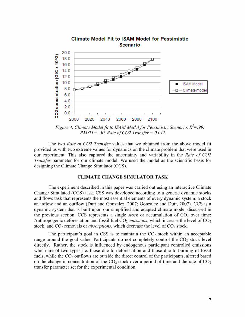
Figure 4. Climate Model fit to ISAM Model for Pessimistic Scenario, R2=.99,

RMSD = .50, Rate of CO2 Transfer = 0.012

The two Rate of CO2 Transfer values that we obtained from the above model fit provided us with two extreme values for dynamics on the climate problem that were used in our experiment. This also captured the uncertainty and variability in the Rate of CO2 Transfer parameter for our climate model. We used the model as the scientific basis for designing the Climate Change Simulator (CCS).

CLIMATE CHANGE SIMULATOR TASK

The experiment described in this paper was carried out using an interactive Climate Change Simulated (CCS) task. CSS was developed according to a generic dynamic stocks and flows task that represents the most essential elements of every dynamic system: a stock an inflow and an outflow (Dutt and Gonzalez, 2007; Gonzalez and Dutt, 2007). CCS is a dynamic system that is built upon our simplified and adapted climate model discussed in the previous section. CCS represents a single stock or accumulation of CO2 over time; Anthropogenic deforestation and fossil fuel CO2 emissions, which increase the level of CO2 stock, and CO2 removals or absorptions, which decrease the level of CO2 stock.

The participant’s goal in CSS is to maintain the CO2 stock within an acceptable range around the goal value. Participants do not completely control the CO2 stock level directly. Rather, the stock is influenced by endogenous participant controlled emissions which are of two types i.e. those due to deforestation and those due to burning of fossil fuels, while the CO2 outflows are outside the direct control of the participants, altered based on the change in concentration of the CO2 stock over a period of time and the rate of CO2 transfer parameter set for the experimental condition.

8

Figure 5 presents the graphical user interface of CCS. The stock is represented in an “atmospheric tank” in continuous units of the stock as CO2 concentration. The markings on the left-hand side of the tank represent the CO2 level in the atmospheric tank at any instance of time. There are 2 pipes connecting the tank, one labeled Emissions, which increases the level of stock in the tank, and other pipe labeled Absorptions, which decreases the level of stock in the tank.

Figure 5. Climate Change Simulator task

Emissions or total emissions are made up of 2 components, fossil fuel emissions and deforestation emissions. The participant must set the fossil fuel and deforestation emissions in the respective text boxes labeled Fossil Fuel Emissions (GtC/year) and Deforestation Emissions (GtC/year), and click the Make Emission Decision button. To avoid extreme exploration of participants’ emission decisions we restricted the fossil fuel and deforestation emissions values to between From and To ranges. Ranges are calculated after each emission decision time step executed by the participant (i.e. after every click of the Make Emission Decision button). The absorption calculations are shown on the graphical user interface as:

Absorptions = Rate of CO2 transfer * (Current CO2 concentration – Preindustrial CO2 concentration) (2)

Thus, absorptions are computed from assumptions of our climate model and are proportional to the current concentration of CO2 i.e. if CO2 concentration is high, the absorptions would also become high and vice versa. The target level of CO2 stock is shown with a green horizontal line with a label Goal. According to attainable goals in IPCC (Houghton, et al. 2001) documents, a Goal level was selected for this task to be 938 GtC.

9

Participants were asked to keep the stock within +/- 15 GtC of the goal (Goal upper bound (GtC) and Goal lower bound (GtC) define the upper and lower bounds of the range around the goal).

For the calculation of the range of values i.e. Goal upper bound (GtC) and Goal lower bound (GtC), we first categorized all the SRES scenarios as for better and for worse based upon whether the net emissions in a particular scenario decreased or kept increasing. We then found the yearly percentage change in fossil fuel and deforestation emissions under for better and for worse scenarios (done separately for both kinds of scenarios). We then picked the lowest five percentage change values and averaged them. Also, we picked the highest five percentage change values and averaged them. This averaging for highest five and lowest five values was done independently for both for better and for worse categories. This averaging exercise gave us two high average values of percentage change and two low averaged values of percentage change for emissions. We picked the maximum of the two high values as the To value and the minimum of the two low values as the From value.

The Year tells the participant what the current time period is out of a total number of years. The information on Fossil Fuel Emissions, Deforestation Emissions and Total Emissions, next to Emissions pipe, inform the participant of the emission values that the participant inputted in the previous time period for fossil fuel and deforestation emission constituents. The absorptions information display provides information on value of absorption at each time step that occurred in the previous time period and the method of calculation of CO2 absorptions. The Current CO2 concentration can be either read using the left scale provided on atmospheric tank or can be seen displayed on a label above the tank. There are three graphical information displays provided at the bottom of the tank. The left most shows the current and past CO2 concentrations over the years up to the current time point in the simulation. The middle graph plots the current and past total CO2 emissions which combine the deforestation and fossil fuel emissions parts. The right graph shows the current and past absorptions of CO2 from the atmospheric tank (notice that as absorptions are proportional to CO2 concentration, this graph has the same shape as the left most CO2 concentration graph). A participant’s goal is to stabilize the CO2 concentration to values within the Goal range with minimum costs incurred. Every time a participant is unable to keep the CO2 concentration in the goal range, he or she incurs a cost penalty which is based on the IPCC documents (Houghton, et al. 2001) denoting damages due to climate problems as $100 million times the difference between the goal and the amount of CO2 in the atmospheric tank. Participants stop incurring cost penalty if they are able to maintain the CO2 concentration within the specified range limits above and below the Goal i.e. the green goal line. The current cost penalty is shown as Current Costs and accumulated penalty as the Total Costs on the information display.

In CCS, participants decide on deforestation and fossil fuel emissions and click the Make Emission Decision button. This causes the climate simulator to move autonomously by a number of time steps to a future year with changes to CO2 stock and CO2 absorptions. During each of these transit years until the system stops in some future year, the total user emissions are the same in each transit year and their value equals the values entered by

10

participants before clicking the Make Emission Decision button. When the system stops, a participant can again decide on total emission values based on the current state of the system and its history over all the past years. This process carries on until the end year in the simulation is reached. In the next section, we describe an experiment conducted using the climate change model and the CCS task.

EXPERIMENT

The Optimistic and Pessimistic scenarios of future emissions proposed by the IPCC (Houghton, et al. 2001) were tested experimentally using the CCS task. As explained earlier, two rates of transfer result from these two scenarios: 1.6% and 1.2% per year for the Optimistic and Pessimistic scenarios respectively.

In the presence of slower dynamic condition (1.2% rate of CO2 transfer) where there is more delay in emissions decisions (made every 4 years), we expected participants to be unable to control the climate system and show poor control performance or higher discrepancy (i.e. difference between the goal and amount of CO2 stock) over many years. On the other hand, a participant’s performance in the face of a rapid climate dynamic condition (1.6% rate of CO2 transfer and emissions decisions made every 2 years) should be better with lower discrepancy. On account of greater delay in the slower dynamic condition, we expected to find oscillations or bullwhips in the discrepancy stock. Also, on account of the presence of time delay in both slow and rapid conditions, we expected that the mean value of total participant emissions under the two conditions would be significantly different from their respective optimal values (or the difference between the optimal and observed values of total emissions would be significantly different from 0). This would be primarily on account of a participant’s inability to take into account the feedback delays and non linearity in general of dynamic problems.

Methods

Experimental Design

In this experiment, we controlled for the Rate of CO2 transfer parameter and the frequency of deforestation and fossil fuel emission decisions and asked participants to attempt to control the system over the course of 50 decision points. Specifically, participants worked on one of two extreme scenarios: one rapid, where rate of CO2 transfer is 1.6% per year with CO2 emission decisions made every 2 years, and other slow, where rate of CO2 transfer is 1.2% per year with CO2 emission decisions made every 4 years. The goal was to maintain the level of CO2 within +/- 15 GtC from the 938 GtC goal (i.e. 923 GtC to 953 GtC). We ran the rapid condition for 100 years and the slow condition for 200 years to equalize the number of decisions made in both conditions to 50 decisions in order to be able to compare both the conditions for results. We started CCS in the year 2000 where the initial CO2 concentration was fixed at 769 GtC. The value of 769 GtC was obtained using the average of the values from all 12 IPCC SRES scenarios (Jain, et al. 1994). Incidentally, all SRES scenarios predicted a value close to 769 GtC for year 2000

11

CO2 concentration. Similarly, the initial deforestation emissions for year 2000 were fixed at 1.3 GtC/year and the initial fossil fuel emission was fixed at 6.88 GtC/year.

The From and To ranges of fossil fuel emissions was set at -14% to +22% of the value of current fossil fuel emissions. Also, for deforestation emissions, the From and To ranges were set as -51% to +55% of the value of current deforestation emissions.

In both slow and rapid dynamic conditions for reaching and stabilizing CO2 to the goal, the total emissions should equal total absorptions when we reach and stabilize CO2 to the goal. This means that for the slow condition, the optimal value of total emissions equals (938 – 677) * 0.012 = 2.952 GtC per year. Similarly, for the rapid dynamic condition, the optimal value of total emissions equals (938 – 677) * 0.016 = 3.936 GtC per year. Thus, if a participant is able to decrease total emissions from their year 2000 value of 8.18 GtC per year (i.e. 6.88 GtC per year for fossil fuel + 1.30 GtC per year for deforestation) to the corresponding lower optimal values under the two conditions, then the participant would be able to hit the goal and stabilize the CO2 concentration to the goal.

We used the absolute value of the difference between the goal and the concentration of CO2 in the atmospheric tank i.e. the discrepancy as the dependent variable for the purpose of statistical analysis. Also, we used the difference between average total emissions under each condition and its optimal emission value as the dependent variable (we call this variable discrepancy in emissions from optimal).

Participants

Eighteen graduate and undergraduate students from diverse fields of study

participated in this experiment. 10 were females, and 8 were males. Ages ranged from 18 years to 31 years with an average age of 23 years. Eight participants were randomly assigned to the slow dynamic condition and ten participants were randomly assigned to the rapid dynamic condition. All participants received a base pay of $5. The participants could earn an additional bonus out of a maximum of $3, based on their performance in the CCS task. The calculation of performance bonus was tied to the cost incurred by a linear relationship. Each time a participant could not keep the CO2 stock between +/- 15 GtC above or below the goal of 938 GtC in the CO2 atmospheric tank (i.e. the CO2 stock level did not lay between 923 GtC and 953 GtC), the participant incurred a cost which was $100 million times the discrepancy between the upper or lower bound of the goal and the CO2 concentration stock. Cost incurred was $0 if the participant was able to control the CO2 concentration stock to stabilize it between 923 GtC and 953 GtC. Participants got $3 in performance bonus if they could keep the total costs in the task to be less than or equal to $15 billion. Participants got $0 in performance bonus (i.e. only got the base pay) if they incurred a total cost of $400 billion or more. For total costs between $400 billion and $15 billion the cost was linearly translated to give a bonus which lay between $0 and $3.

Procedure

Participants were randomly assigned to one of the two conditions (i.e. slow or rapid), and they were given instructions on the computer before starting the CCS task. Text of the instruction for both conditions is detailed in Appendix B. Soon after participants read

12

the instructions, they were shown a 50 year status quo scenario in CCS. This scenario demonstrated what the state of affairs would be if no action had been taken at all in the simulation. This scenario started in the year 2000 and ended in year 2050. In this scenario, the year 2000 emissions for deforestation were maintained at 1.3 GtC per year and the emissions for fossil fuels at 6.88 GtC per year for the next 50 years (these values of emissions are actually the year 2000 or status quo values). Starting with year 2000 concentrations of 769 GtC (from climate model), the concentration of CO2 in the atmospheric tank increased to more than 1000 GtC by year 2050, which is more than a 5% increase from the year 2000 value. Participants were told of the severe consequences that this increase in concentration might hold in terms of economic and human losses. After the scenario finished, participants were encouraged to ask questions on the task. Participants were given full information on the CCS task and were reminded that their task was to control CO2 concentration to within the +/- 15 GtC range around the goal over the entire course of the CCS task. They were then asked to play the CCS task for 50 decision points over a course of 100 or 200 years depending upon the randomly assigned condition.

Participants sat in front of a computer screen and were presented with the CCS displayed in the center of the screen. We made use of Windows XP-based desktop computer terminals with plasma screens, which had a resolution of 1024 x 1080; the desktop computers ran on a Pentium 4 processor base.

Results The distribution for the discrepancy in the data for both slow and rapid dynamic

conditions as a whole was found to be non-normal in K-S tests. We tested for normality of the data on the 1st decision point, 25th decision point and the 50th decision point. For the 1st decision point the data was normal for both the slow and rapid conditions, D(8) = .250, ns and D(10) = .180, ns respectively.1 For the 25th decision point, the data was non-normal for the slow condition but was normal for the rapid condition with D(8) = .324, p <.05 and D(10) = .178, ns respectively. Lastly, for the 50th decision point, the data was non-normal for both slow and rapid conditions with D(8) = .346, p <.05 and D(10) = .285, p <.05 respectively. Also, Levene’s test for homogeneity of variances for the data revealed that for 1st and 50th decision points, the variance in the data were homogenous F (1, 16) = 1.131, ns, and F (1, 16) = 2.104, ns respectively. But Levene’s test for the homogeneity of variances for the 25th decision point indicated that the variances to be significantly different, hence the assumptions of homogeneity of variances had been violated, F (1, 16) = 5.624, p <.05. Due to non-normality and non-homogeneity of variances across decision points we report non parametric statistics here.

The Mann-Whitney test reported that the discrepancy in the slow dynamic condition (Mean =96.10 GtC; Std. Dev. =142.83 GtC) was significantly higher than the discrepancy in the rapid dynamic condition (Mean =50.38 GtC; Std. Dev. =42.65 GtC) with U = 86084,

1 The value D(8) means degree of freedom of 8. This implies that for the 1st decision points, we had in all 8 participants in slow condition. Similarly, D(10) means 10 participants in the rapid condition for the 1st decision point.

13

Z = -3.59, p < .001, r = -.12. Figure 6 shows the discrepancy in both the slow and rapid dynamic conditions. From Figure 6, it is easy to see the oscillatory nature of the Discrepancy in CO2 concentration in the slow dynamic condition as compared to the rapid dynamic condition.

Figure 6. Discrepancy in CO2 concentration between slow and rapid conditions

To test for improvement of performance (or learning) across decision points within both the slow and rapid dynamic conditions, Wilcoxon test was performed. For participants in the slow dynamic condition, the discrepancy was significantly higher on the 1st decision point (Mean =162.78 GtC; Std. Dev. =.71 GtC) than the 50th decision point (Mean =58.04 GtC; Std. Dev. =103.62 GtC), T = 3, p < .05, r = -.47. Also, for participants in the rapid dynamic condition, the discrepancy was significantly higher on the 1st decision point (Mean =162.35 GtC; Std. Dev. =1.23 GtC) than the 50th decision point (Mean =28.74 GtC; Std. Dev. =33.85 GtC), T = 0, p < .05, r = -.63. This result shows that participants showed learning or improvement in performance over time.

To test whether the total emissions (i.e. sum of fossil fuel and deforestation emissions) under slow and rapid conditions were significantly different from their optimal values, we compared the discrepancy in emissions from the optimal dependent variable with a 0 value in a Mann-Whitney test for both conditions separately. The Mann-Whitney test reported that the discrepancy in emissions from optimal in the slow dynamic condition (Mean =1.28 GtC per year; Std. Dev. =1.43 GtC per year) was significantly higher than 0 values (Mean =0 GtC per year; Std. Dev. =0 GtC per year) with U = 183.5, Z = -7.47, p < .001 r = -.74. Also, the Mann-Whitney test reported that the discrepancy in emissions from optimal in the rapid dynamic condition (Mean =1.36 GtC per year; Std. Dev. =1.68 GtC per year) was significantly higher than 0 values (Mean =0 GtC per year; Mdn = 0 GtC per year)

14

with U = 150, Z = -8.11, p < .001 r = -.81. Results indicate presence of suboptimal performance in both conditions and support for our expectation on emission hypothesis.

Lastly, the Mann-Whitney test reported that the discrepancy in emissions from optimal in the slow dynamic condition (Mean =1.28 GtC per year; Std. Dev. =1.43 GtC per year) was not significantly different than the discrepancy in emissions in the rapid dynamic condition (Mean =1.36 GtC per year; Std. Dev. =1.68 GtC per year) with U = 1218, Z = -0.22, ns. This result shows that performance on emission decisions was generally poor and similar under both conditions. Figure 7 shows the total emissions for participants under both the slow and rapid conditions. From figure 7, it can be seen that rapid emissions are higher in value than slow emissions (although this difference is insignificant). The higher value of emissions in rapid dynamic condition than slow dynamic condition produces more CO2 stock under rapid than slow condition. As the CO2 absorption from atmospheric tank is a function of CO2 stock, the higher CO2 stock under rapid dynamic condition leads to higher absorption rate (outflow) causing a greater lowering in stock and lesser discrepancy in rapid dynamic condition than the discrepancy in slow dynamic condition (as seen in Figure 6).

Figure 7. Total Emissions in slow and rapid dynamic conditions

DISCUSSION AND CONCLUSIONS Many of the complex dynamic effects found in the real world can be better

understood with simple tasks (Cronin et al. in press) and here we present a demonstration of such a process in CSS. The focus of this is on the simplification of a complex problem such as global warming into one of the most important elements of the problem: the human understanding of accumulation and depletion of stocks over time. We varied the dynamics of the climate system and the frequency of emission decisions. Participants showed poor selection of emission decisions in both slow and rapid conditions and show an evidence of

15

bullwhip like oscillations and higher discrepancy for slower dynamics in terms of smaller CO2 absorptions rates. Such bullwhip oscillations and higher discrepancy due to faulty total emission decisions by humans could have drastic social, economic and political consequences.

As already mentioned, the problem of human understanding and control of dynamic systems, such as the climate change, is widely known (Sweeney and Sterman 2000; Brehmer 1989, 1992; Diehl and Sterman 1995; Moxnes and Saysel 2004; Paich and Sterman 1993; Sterman 1989; Sterman and Sweeney 2002). But recently, evidence for an even more disturbing problem has been found: that people have trouble understanding even simple dynamic tasks consisting of one stock, one inflow and one outflow (Cronin and Gonzalez 2007; Cronin, et al. in press). When people are encountered by problems in these systems, they, due to cognitive incapacities, simply fail to account for non linearity, feedback delays and side effects. Although, the slow dynamic condition offers twice the delay in human decisions than the rapid dynamic condition, the rapid dynamic is also delayed (by two time periods). Also, in the slower dynamic condition, the absorption non linearity and side effects are only 0.4% less than the rapid dynamic condition (i.e. 1.6% in rapid dynamic condition minus the 1.2% in slow dynamic conditions). Thus, participants who received either of the two conditions, slow or rapid, due to human cognitive inabilities won’t be able to understand the consequences of their actions, won’t foresee how the system would evolve simply because they suffer from poor system’s thinking as a result of their limited cognitive capacities and this leads to poor control and performance under both dynamic conditions.

We believe that due to the poor participant performance there is a strong evidence for faulty system’s thinking on part of our participants and support for “Misperceptions Of Feedback” (MOF) hypothesis (Sterman, 1989) exists in our research study. In our study, the slow condition has four units of time delay which is twice the delay in rapid condition where the slow condition accompanies slower system dynamics than the rapid condition. Under these conditions, although all features of the climate change task are transparent and salient, yet people simply fail to account for time delays and dynamic complexity due to their limited mental models and cognitive incapacities and this leads to bullwhip like oscillation in the slow dynamic condition. Diehl and Sterman (1995) reported the effect of variation of dynamic complexity on human performance in a first order dynamic decision making task where the task was to minimize cost in the system by controlling stock in a bathtub to a desired level. In their task participants made production decisions where the sales (outflow) of the system were a function of both the production (i.e. participant controlled inflow) and an exogenous noise. According to Diehl and Sterman (1995), there was a large deterioration of control performance with increase in feedback delay where participant’s stock showed oscillations which were directly proportional to delay in the production decisions. The primary reason for the poor participant performance was attributed of the “Misperceptions of Feedback” (MOF) hypothesis (Sterman, 1989), where people took an “open loop” view of an actual closed loop system, failed to account for feedback delays between actions and responses, did not comprehend the system dynamics and ignored the non linearity present in the system.

16

We also find an explanation for poor participant control performance in our climate change task under both slow and rapid conditions from experiments reported using a single player beer game by Martin and Gonzalez (under review). According to Martin and Gonzalez (under review), the bullwhip effect, i.e. the increase in oscillation in inventory stock, was found to be directly proportional to the lead time in terms of ordering and shipping delay in the beer distribution game. People simply ignored the supply line of the beer and mostly concentrated to keep their own inventory at a higher level. This neglect of the supply line led to bullwhip like oscillations due to the working of MOF hypothesis. When Martin and Gonzalez (under review) experimentally increase the ordering and shipping delay in weeks for procuring beer after placing an order, participants experienced more bullwhip. This finding applies directly to the current results for the climate system and forms an explanation for the presence of a bullwhip like oscillation in the CO2 stock for the slow condition compared to the CO2 stock in the rapid dynamic condition. We varied the frequency of CO2 emissions decisions made by the participants under the two different dynamic conditions. The frequency of emissions decisions between the slow and rapid conditions are the year gaps between decision points at which participants can order new CO2 emissions. Participants cannot alter emissions on any year between any two decision points. Increasing the frequency of decisions i.e. the time gap between two decision points is similar to increasing the shipping and ordering delay in a single player Beer Game (Martin and Gonzalez, under review). Thus, in slow dynamic conditions where people find a feedback delay of four years between two consecutive decision points, they tend to neglect this delay in emissions due to their cognitive incapacities and misperceptions of feedback. This results in bullwhip oscillations under slow conditions of feedback delay. On the other hand, for the rapid dynamic condition, the frequency of emission decisions is double and dynamics is rapid resulting is lesser feedback delay and better human performance.

In our experiment, participants made poor total emissions decisions under both conditions which were significantly different from total optimal emissions behavior in the problem under both the conditions. This happened even after the CCS simulation was completely transparent to the participants i.e. we provide participants with full details on the dynamics of problem, and there was no time pressure on the participants in the task. The support for the finding comes from the account for human cognitive incapacities in face of dynamic complexities as reported by Diehl and Sterman (1995). Diehl and Sterman (1995) report that in a first order system like our climate system, participant’s ordering (i.e. inflow) decisions were poor and directed away from optimal behavior. The only condition where participants performed well was when the system did not have any side effects or feedback time delays: i.e. the simplest control condition. Under this control condition participants showed good performance with near optimal control as they did not encounter any MOF because there were no system delays. Under such conditions of no delay and no side effects a participant could simply turn off the production once the goal was attained and the system would behave optimally and instantaneously to participant’s commands. We argue that due to the presence of delays in both of the dynamic conditions in our climate task, following such a simple “turn off emissions” strategy would not provide better control and would continue to pose problems in system control. We cannot simply shut down the

17

emissions or drastically decrease them from high values when the CO2 concentration reaches the goal because by that time it is already too late to do so due to slow feedback delays governing the system: the climate system is slow with longer time delays between actions and their consequences. Even if we were able to completely shut down the total CO2 emissions from a high value to 0 as the concentrations of CO2 reached the goal, the concentration of CO2 would continue to rise and overshoot the goal due to the ordered emissions still pending to occur and also due to the low absorptions of CO2.

We have already shown in this paper that in both dynamic conditions, the optimal strategy, or the correct thing to do is to slowly reduce the CO2 emissions from there year 2000 value of 8.18 GtC per year down to where they become equal to absorptions and the system reaches the goal concentration of CO2. This optimal decrease in the case of the slow and rapid dynamic conditions has to be from 8.18 GtC per year to 2.952 GtC per year and 3.936 GtC per year respectively. Thus, simply stated in our task the optimal strategy is to slowly decrease the velocity of emissions i.e. to reduce emissions and make them approach the absorptions when the concentration approaches the goal. Participants although try to reduce emissions under both conditions but do not follow the optimal strategy to reduce emissions at the correct pace and continue to maintain emissions at higher values than to gradually decrease them till they reach the goal. But by this time, when they are at the goal, it is too late to act or respond to correct their mistake and cut down emissions. This distressing participant emission behavior on account of MOF hypothesis also provides supportive evidence for the “wait and watch” policies currently being followed in the real world for our climate (Sterman and Sweeney 2002). People in today’s world want to continue to maintain emissions at high levels rather than to take actions which are geared towards reducing them. It appears that at the current pace people will continue to hold emissions at higher values till the concentrations of GHGs start overshooting the desirable amounts and goals and only realize the misperceptions of their actions when is already too late to correct their actions due to the delays present in the system (Sterman and Sweeney 2002). The solution to the problem is to make people repeatedly play climate scenarios like ours using climate simulator tools like CCS where people learn to foresee their mistakes with repeated practice and come to realize that the key to the problem of global warming to gradually reduce emissions at the correct pace from their current higher values so that the problem does not lead to catastrophic outcomes for the future.

There are a number of suggestions that come out of this research. Firstly, participants show lower CO2 discrepancy in the rapid dynamic condition than slow dynamic condition. Thus, making rapid emission policy decisions helps to control climate change more successfully than slower policy decisions; our emission policies for climate should be revised periodically and at short periods of time. Secondly, another main intervention is the use of CCS to give training and educate people on the problem. The tool in its simplistic structure is able to make the climate problem understandable to common people and has a potential to increase the human understanding of accumulation and depletion of stocks over time, making them aware of the urgency of the situation before it becomes too late to act to save the Earth from climate change.

18

Our results in this study demonstrate that individuals have lesser discrepancy and bullwhip oscillation in the rapid condition than the slw condition thus participants learn more quickly when the system follows rapid dynamics than slower dynamics. This means that a more frequent repeated policymaking strategy on climate issues would lead to significantly better outcomes than the less frequent policymaking strategy intervention. Results also show that in general, people have great difficulties in understanding and controlling a stock even in simpler dynamic systems consisting of one stock. Individuals were better at controlling the system with shorter decision delays and rapid system response dynamics than their inverse counter parts, supporting previous findings in dynamic systems (Dörner, 1980; Sterman, 1994). The results support our hypothesis and findings from a wide literature on people’s inability to handle dynamically complex systems and people’s reliance on faulty stock – flow heuristics (Brehmer 1989; Cronin, et al. in press; Diehl and Sterman 1995).

We plan to continue our initial research investigations reported in this paper. In particular, it is important to understand the independent effects of the two variables manipulated in this experiment: the dynamics of the system and the feedback. For example, it would be important to see if in the pessimistic scenario more frequent decisions would help in controlling the system compared to less frequent decisions. We see that greater understanding of human incapacities and cognitive limitations using tools like CCS is the right step for research in this endeavor.

ACKNOWLEDGMENTS This research was partially supported by the National Science Foundation (Human

and Social Dynamics: Decision, Risk, and Uncertainty, Award number: 0624228) award to Cleotilde Gonzalez.

19

References

Brehmer, B. 1989. Feedback Delays and Control in Complex Dynamic Systems. International Conference of the System Dynamics Society, Stuttgart, Springer-Verlag.

Brehmer, B. 1992. Dynamic decision making: Human control of complex systems. Acta Psychologica, 81(3), 211-241.

Climate Change Fact Sheet. 2006. Recent Polling on Public Perceptions of Climate Change. Environment and Energy Study Institute. April 2005-2006, Washington DC.

Cronin, M, and C Gonzalez. 2007. Understanding the building blocks of system dynamics. System Dynamics Review 23 (1):1-17.

Cronin, M, C Gonzalez, and J D Sterman. In press. Why don't well-educated adults understand accumulation? A challenge to researchers, educators and citizens. Journal of Organizational Behavior and Human Decision Processes – Elsevier. Forthcoming.

Diehl, E, and J D Sterman. 1995. Effects of feedback complexity on dynamic decision making. Organizational Behavior and Human Decision Processes 62 (2):198-215.

Dörner, D. 1980. On the difficulties people have in dealing with complexity. Simulation and Games, 11(1), 87-106.

Dutt, V., and C Gonzalez. 2007. Slope of inflow impacts dynamic decision making. Paper presented at the System Dynamics Conference. Boston, MA.

Gonzalez C., and V Dutt. In Preparation. Slope of inflow impacts dynamic decision making. Organization Behavior and Human Decision Processes.

Houghton, J. T., Y Ding, D J Griggs, M Noguer, P J van den Linden, X Dai, et al. (Eds.). 2001. Climate change 2001: The scientific basis. Contribution of working group I to the third assessment report of the Intergovernmental Panel on Climate Change. New York: Cambridge University Press.

Jain, A.K., H S Kheshgi, and D J Wuebbles. 1994. Integrated Science Model for Assessment of Climate Change Model presented at and published in the proceedings of Air and Waste Management Association’s 87th Annual Meeting, Cincinnati, Ohio, June 19-24.

Leiserowitz, A A. 2005. American risk perceptions: Is climate change dangerous? Risk Analysis 25 (6):1433-1442.

Leiserowitz, A A. 2006. Climate change risk perception and policy preferences: The role of affect, imagery, and values. Climatic Change 77:45-72.

Martin, M., and C Gonzalez. under review. Learning to control the bullwhip: Dynamic decision making in the beer game.

Moxnes, E. 1998a. Not only the Tragedy of the Commons: Misperceptions of Bioeconomics. Management Science, 44(9): 1234-1248.

Moxnes, E. 1998b. Overexploitation of renewable resources: The role of misperceptions. Journal of Economic Behavior and Organization, 37: 107-127.

Moxnes, E. 2000. Not only the tragedy of the commons: misperceptions of feedback and policies for sustainable development, System Dynamics Review, 16(4), 325-348.

20

Moxnes, E. 2004. Misperceptions of basic dynamics: The case of renewable resource management. System Dynamics Review 20 (2):139-162.

Moxnes, E, and A K Saysel. 2004. Misperceptions of global climate change: Information policies. Bergen, Norway: University of Bergen.

Nebojs¢a, N., D Ogunlade, et al. 2000. Summary for Policymakers. Emissions Scenarios: A Special Report of Working Group III of the Intergovernmental Panel on Climate Change.

Nodhaus, W D. 1992. The “DICE” Model: Background and Structure Of a Dynamic Integrated Climate Economy Model of Economics of Global Warming. Cowles Foundation Discussion Paper 1009. Cowles Foundation for Research in Economics At Yale University. New Haven, Connecticut.

OakRidgeNationalLaboratory. 1990. Glossary: Carbon Dioxide and Climate, Carbon Dioxide Information Analysis Center, Oak Ridge National Laboratory, Oak Ridge, Tennessee.

Paich, M, and J D Sterman. 1993. Boom, bust and failures to learn in experimental markets. Management Science 39 (12):1439-1458.Sterman, J D. 1989. Misperceptions of feedback in dynamic decision making. Organizational Behavior and Human Decision Processes 43 (3):301-335.

Sterman, J D. 1989. Misperceptions of feedback in dynamic decision making. Organizational Behavior and Human Decision Processes 43 (3):301-335.

Sterman, J D. 1994. Learning in and about complex systems. System Dynamics Review 10:291-330.

Sweeney, L B, and J D Sterman. 2000. Bathtub dynamics: Initial results of a systems thinking inventory. System Dynamics Review 16 (4):249-286.

Sterman, J D, and L B Sweeney. 2002. Cloudy skies: Assessing public understanding of global warming. System Dynamics Review 18 (2):207-240.

Sterman, J D, andand L B Sweeney. 2007. Understanding public complacency about climate change: Adults' mental models of climate change violate conservation of matter. Climatic Change, 80(3-4), 213-238.

21

Appendix A

Vensim® PLE Equations for System Dynamics Climate Model

(01) CO2 emissions into Atmosphere= User Action CO2 emissions Units: TonC/Year [0,1e+012] (02) CO2 in Atmos= INTEG (CO2 emissions into Atmosphere-CO2 removals, 7.69e+011)

Units: TonC (03) CO2 removals= (CO2 in Atmos-Preindustrial CO2)*Rate of CO2 Transfer Units: TonC/Year (04) FINAL TIME = 2100

Units: Year The final time for the simulation. (05) INITIAL TIME = 2000 Units: Year The initial time for the simulation. (06) Preindustrial CO2= 6.77e+011 Units: TonC (07) Rate of CO2 Transfer= 0.012 Units: 1/Year

Rate of Storage of Atmospheric Greenhouse Gases [delta-m] (1/year) Inverse yields average residence time of gases (120 years).

(08) SAVEPER = 5 Units: Year [0,?] The frequency with which output is stored. (09) TIME STEP = 10 Units: Year [0,?] The time step for the simulation. (10) User Action CO2 emissions Units: TonC/Year

We define different user inflow actions here (SRES Scenarios A2 and B1 were defined here for our model fits)

22

Appendix B

Instructions for Slow Dynamic Condition

The only change in text for the instructions given in the Rapid Dynamic Condition was making the end year as 2100 (in place of 2200), the frequency of emission decisions to be every 2 years (in place of every 4 years) and the absorptions to be 1.6% of the difference between the current CO2 concentration and the preindustrial CO2 concentration (in place of 1.2%).

23

24

25

26