human and ecological risk assessment of coal combustion wastes
TRANSCRIPT

Human and Ecological Risk Assessment of
Coal Combustion Wastes
Draft
Prepared for:
U.S. Environmental Protection Agency Office of Solid Waste
Research Triangle Park, NC 27709
Prepared by:
RTI P.O. Box 12194
Research Triangle Park, NC 27709
August 6, 2007


Human and Ecological Risk Assessment of Coal Combustion Wastes
Draft EPA document. Do not cite or quote.
Human and Ecological Risk Assessment of
Coal Combustion Wastes
Prepared for:
U.S. Environmental Protection Agency
Office of Solid Waste Research Triangle Park, NC 27709
Prepared by:
RTI P.O. Box 12194
Research Triangle Park, NC 27709
August 6, 2007

Human and Ecological Risk Assessment of Coal Combustion Wastes
Draft EPA document. Do not cite or quote.
[This page intentionally left blank.]

Human and Ecological Risk Assessment of Coal Combustion Wastes Table of Contents
Draft EPA document. Do not cite or quote. iii
Table of Contents Section Page Executive Summary ...................................................................................................................ES-1
1.0 Introduction...................................................................................................................... 1-1 1.1 Background.......................................................................................................... 1-1 1.2 Purpose and Scope of the Risk Assessment......................................................... 1-2 1.3 Overview of Risk Assessment Methodology....................................................... 1-2
1.3.1 Waste Management Scenarios ................................................................. 1-5 1.3.2 Approach.................................................................................................. 1-5
1.4 Document Organization ....................................................................................... 1-6
2.0 Problem Formulation ....................................................................................................... 2-1 2.1 Source Characterization ....................................................................................... 2-1
2.1.1 Identification of Waste Types, Constituents, and Exposure Pathways .................................................................................................. 2-2
2.1.2 Waste Management Scenarios ................................................................. 2-5 2.2 Conceptual Model................................................................................................ 2-8
2.2.1 Conceptual Site Model............................................................................. 2-8 2.2.2 Conceptual Site Layouts ........................................................................ 2-10
2.3 Analysis Scope and Design................................................................................ 2-13 2.3.1 Data Collection ...................................................................................... 2-14 2.3.2 Model Implementation........................................................................... 2-15 2.3.3 Exposure Assessment............................................................................. 2-16 2.3.4 Risk Estimation...................................................................................... 2-17
3.0 Analysis............................................................................................................................ 3-1 3.1 General Modeling Approach................................................................................ 3-2
3.1.1 Temporal and Spatial Framework............................................................ 3-2 3.1.2 Probabilistic Approach............................................................................. 3-4 3.1.3 Implementation of Probabilistic Approach.............................................. 3-6
3.2 Landfill Model ..................................................................................................... 3-8 3.2.1 Conceptual Model.................................................................................... 3-9 3.2.2 Modeling Approach and Assumptions................................................... 3-10 3.2.3 Landfill Model Input Parameters ........................................................... 3-13 3.2.4 Model Outputs ....................................................................................... 3-15
3.3 Surface Impoundment Model ............................................................................ 3-15 3.3.1 Conceptual Model.................................................................................. 3-15 3.3.2 Modeling Approach and Assumptions................................................... 3-17 3.3.3 Surface Impoundment Model Input Parameters .................................... 3-18 3.3.4 Surface Impoundment Model Outputs................................................... 3-20
3.4 Groundwater Model ........................................................................................... 3-21 3.4.1 Conceptual Model.................................................................................. 3-21 3.4.2 Modeling Approach and Assumptions................................................... 3-22 3.4.3 Model Inputs and Receptor Locations ................................................... 3-23 3.4.4 Groundwater Model Outputs ................................................................. 3-25

Human and Ecological Risk Assessment of Coal Combustion Wastes Table of Contents
Draft EPA document. Do not cite or quote. iv
3.5 Surface Water Models........................................................................................ 3-25 3.5.1 Equilibrium Partitioning Model............................................................. 3-25 3.5.2 Aquatic Food Web Model...................................................................... 3-27 3.5.3 Aluminum Precipitation Model ............................................................. 3-28
3.6 Human Exposure Assessment............................................................................ 3-29 3.6.1 Receptors and Exposure Pathways ........................................................ 3-29 3.6.2 Exposure Factors.................................................................................... 3-30 3.6.3 Dose Estimates....................................................................................... 3-32
3.7 Toxicity Assessment .......................................................................................... 3-33 3.7.1 Human Health Benchmarks ................................................................... 3-34 3.7.2 Ecological Benchmarks ......................................................................... 3-35
3.8 Risk Estimation.................................................................................................. 3-38 3.8.1 Human Health Risk Estimation ............................................................. 3-38 3.8.2 Ecological Risk Estimation.................................................................... 3-40
4.0 Risk Characterization....................................................................................................... 4-1 4.1 Human Health Risks ............................................................................................ 4-2
4.1.1 Groundwater-to-Drinking-Water Pathway .............................................. 4-2 4.1.2 Groundwater-to-Surface-Water (Fish Consumption) Pathway ............... 4-8 4.1.3 Results by Waste Type/WMU Scenario ................................................ 4-10 4.1.4 Results by Unit Type ............................................................................. 4-16 4.1.5 Constituents Not Modeled in the Full-Scale Assessment ...................... 4-18
4.2 Ecological Risks................................................................................................. 4-20 4.2.1 Surface Water Receptors........................................................................ 4-20 4.2.2 Sediment Receptors ............................................................................... 4-21 4.2.3 Constituents Not Modeled in the Full-Scale Assessment ...................... 4-22
4.3 Sensitivity Analysis ........................................................................................... 4-24 4.4 Variability and Uncertainty................................................................................ 4-25
4.4.1 Scenario Uncertainty.............................................................................. 4-26 4.4.2 Model Uncertainty ................................................................................. 4-28 4.4.3 Parameter Uncertainty and Variability .................................................. 4-30
4.5 Summary and Conclusions ................................................................................ 4-38
5.0 References........................................................................................................................ 5-1
Appendix A Constituent Data.................................................................................................. A-1 Appendix B Waste Management Units ....................................................................................B-1 Appendix C Site Data...............................................................................................................C-1 Appendix D MINTEQA2 Nonlinear Sorption Isotherms........................................................ D-1 Appendix E Surface Water, Fish Concentration, and Contaminant Intake Equations.............E-1 Appendix F Human Exposure..................................................................................................F-1 Appendix G Human Health Benchmarks ................................................................................ G-1 Appendix H Ecological Benchmarks ...................................................................................... H-1

Human and Ecological Risk Assessment of Coal Combustion Wastes Table of Contents
Draft EPA document. Do not cite or quote. v
List of Figures Figure Page
1-1. Overview of coal combustion waste risk assessment. ..................................................... 1-4 2-1. Conceptual site model of CCW risk assessment.............................................................. 2-9 2-2. Conceptual site layout for residential groundwater ingestion scenario. ........................ 2-11 2-3. Conceptual site layout for residential fisher and aquatic ecological risk scenario. ....... 2-12 3-1. Overview of the Monte Carlo approach........................................................................... 3-4 3-2. Monte Carlo looping structure. ........................................................................................ 3-5 3-3. Process used to construct the Monte Carlo input database. ............................................. 3-7 3-4. Conceptualization of a landfill in the landfill source-term model. .................................. 3-9 3-5. Schematic cross-section view of surface impoundment. ............................................... 3-16 3-6. Conceptual model of the groundwater modeling scenario. ........................................... 3-21 3-7. Schematic plan view showing contaminant plume and receptor well location. ............ 3-24 4-1. Full-scale 90th percentile risk results for the groundwater-to-drinking-water
pathway. ........................................................................................................................... 4-5 4-2. Full-scale 50th percentile risk results for the groundwater-to-drinking-water
pathway. ........................................................................................................................... 4-6 4-3. Comparison of peak arrival times for arsenic for CCW landfills and surface
impoundments.................................................................................................................. 4-8 4-4. Comparison of risk results for arsenic III and arsenic V (based on results for all
units combined).............................................................................................................. 4-30 4-5. Comparison of CCW leachate data with other leachate data......................................... 4-32 4-6. CCW mercury concentrations compared with other leachate data. ............................... 4-35
List of Tables Table Page
1-1. Liner Prevalence in EPRI and DOE Surveys................................................................... 1-2 2-1. Waste Streams in CCW Constituent Database ................................................................ 2-3 2-2. Toxicity Assessment of CCW Constituents..................................................................... 2-4 2-3. Screening Analysis Results: Selection and Prioritization of CCW Constituents for
Further Analysis............................................................................................................... 2-6 2-4. Coal Combustion Plants with Onsite CCW WMUs Modeled in the Full-Scale
Assessment....................................................................................................................... 2-8 2-5. Receptors and Exposure Pathways Addressed in the Full-Scale CCW Assessment ..... 2-16 3-1. CCW Waste Management Scenarios Modeled in Full-Scale Assessment ...................... 3-6 3-2. Leak Detection System Flow Rate Data Used to Develop Landfill Composite
Liner Infiltration Rates................................................................................................... 3-12 3-3. Crosswalk Between EPRI and CCW Source Model Liner Types ................................. 3-14 3-4. Sediment/Water Partition Coefficients: Empirical Distributions .................................. 3-26 3-5. Bioconcentration Factors for Fish.................................................................................. 3-27 3-6. Aluminum Solubility as a Function of Waterbody pH .................................................. 3-28

Human and Ecological Risk Assessment of Coal Combustion Wastes Table of Contents
Draft EPA document. Do not cite or quote. vi
3-7. Receptors and Exposure Pathways ................................................................................ 3-30 3-8. Human Exposure Factor Input Parameters and Data Sources ....................................... 3-31 3-9. Human Health Benchmarks Used in the Full-Scale Analysis ....................................... 3-35 3-10. Ecological Receptors Assessed by Exposure Route and Medium (Surface Water
or Sediment)................................................................................................................... 3-36 3-11. Ecological Risk Criteria Used in the Full-Scale Analysis ............................................. 3-37 3-12. Risk Endpoints Used for Human Health........................................................................ 3-38 4-1. Summary of 90th Percentile Full-Scale CCW Human Risk Results: Groundwater-
to-Drinking-Water Pathway............................................................................................. 4-3 4-2. Summary of 50th Percentile Full-Scale CCW Human Risk Results: Groundwater-
to-Drinking-Water Pathway............................................................................................. 4-4 4-3. Summary of 90th Percentile Full-Scale CCW Human Risk Results: Groundwater-
to-Surface-Water (Fish Consumption) Pathway.............................................................. 4-9 4-4. Summary of 50th Percentile Full-Scale CCW Human Risk Results: Groundwater-
to-Surface-Water (Fish Consumption) Pathway............................................................ 4-10 4-5. 90th Percentile Risk Results by CCW Type: Landfills, Groundwater-to-Drinking-
Water Pathway ............................................................................................................... 4-11 4-6. 50th Percentile Risk Results by CCW Type: Landfills, Groundwater-to-Drinking-
Water Pathway ............................................................................................................... 4-12 4-7. 90th Percentile Risk Results by CCW Type: Surface Impoundments,
Groundwater-to-Drinking-Water Pathway .................................................................... 4-13 4-8. 50th Percentile Risk Results by CCW Type: Surface Impoundments,
Groundwater-to-Drinking-Water Pathway .................................................................... 4-14 4-9. 90th Percentile Risk Results for FBC Wastes: Landfills, Groundwater-to-
Drinking-Water Pathway ............................................................................................... 4-15 4-10. 50th Percentile Risk Results for FBC Wastes: Landfills, Groundwater-to-
Drinking-Water Pathway ............................................................................................... 4-16 4-11. Unit Types in EPRI Survey............................................................................................ 4-17 4-12. Risk Attenuation Factora Statistics for Modeled Constituents— Groundwater to
Drinking Water Pathway................................................................................................ 4-19 4-13. Summary of Risk Results for Constituents Using Risk Attenuation Factors—
Groundwater-to-Drinking-Water Pathway .................................................................... 4-19 4-14. Summary of Full-Scale CCW Ecological Risk Results: Groundwater-to-Surface-
Water Pathway, Aquatic Receptorsa.............................................................................. 4-21 4-15. Summary of Full-Scale CCW Ecological Risk Results: Groundwater-to-Surface-
Water Pathway, Sediment Receptorsa ........................................................................... 4-22 4-16. Risk Attenuation Factora Statistics for Modeled Constituents— Ecological Risk,
Surface Water Pathway.................................................................................................. 4-23 4-17. Summary of Risk Results Using Risk Attenuation Factors— Ecological Risk,
Surface Water Pathway.................................................................................................. 4-23 4-18. Proportion of Nondetect Analyses for Modeled CCW Constituents ............................. 4-34

Executive Summary Human and Ecological Risk Assessment of Coal Combustion Wastes
Draft EPA document. Do not cite or quote. ES-1
Human and Ecological Risk Assessment of Coal Combustion Wastes – Executive Summary
The U.S. Environmental Protection Agency (EPA) is evaluating management options for solid wastes from coal combustion (e.g., fly ash, bottom ash, slag). As part of this effort, EPA is evaluating whether current management practices for coal combustion waste (CCW) pose risks to human health or ecological receptors. To inform this objective, EPA has conducted a nationwide assessment of the risks posed by CCW disposal practices across the country.
This report describes the results of the tiered, site-based, probabilistic (Monte Carlo) risk assessment of onsite CCW disposal practices at coal-fired power plants across the United States. These landfills and surface impoundments represent disposal practices for CCW reported in 1995. Although EPA acknowledges that management practices for CCW have improved since 1995, as documented in U.S. Department of Energy (DOE) (2006), EPA believes that characterizing risks from facilities observed in 1995 provides a snapshot of the potential risks from CCW disposal and can provide useful information as EPA evaluates CCW management options. In addition, the data available on these facilities’ locations, environmental characteristics, and waste management units (WMUs) allow EPA to apply a site-based risk assessment approach that the agency believes characterizes the risks to human health and the environment from disposing CCW in landfills and surface impoundments.
In summary, this CCW risk assessment evaluates potential risk results at the 50th and 90th percentile exposure level, adopting a risk criteria of 10-5 for excess cancer risks. Potential noncancer and ecological risks are also evaluated at the 50th and 90th percentile levels, adopting a hazard quotient (HQ) risk criteria greater than 1 for noncancer effects to both human and ecological receptors. Overall, when all types of landfills and surface impoundments (as observed in 1995) are evaluated in aggregate, the risk at the 90th percentile exceeds the risk
criteria for cancer and noncancer risks for certain constituents. There is no potential risk above the risk criteria (cancer and noncancer) found at the 50th percentile. The risk assessment also suggests that one of the most sensitive parameters in the risk assessment is infiltration rate. Infiltration rate is greatly influenced by whether and how a WMU is lined.
For humans exposed via the groundwater-to-drinking-water pathway, arsenic in CCW landfills poses a 90th percentile cancer risk of 5x10⁻⁴ for unlined units and 2x10⁻⁴ for clay-lined units. The 50th percentile risks are 1x10⁻⁵ (unlined units) and 3x10⁻⁶(clay-lined units). Risks are higher for surface impoundments, with an arsenic cancer risk of 9x10⁻³ for unlined units and 3x10⁻³ for clay-lined units at the 90th percentile. At the 50th percentile, risks for unlined surface impoundments are 3x10⁻⁴, and clay-lined units show a risk of 9x10⁻⁵. Five additional constituents have 90th percentile noncancer risks above the criteria (HQs ranging from greater than 1 to 4) for unlined surface impoundments, including boron and cadmium, which have been cited in CCW damage cases, referenced above. Boron and molybdenum show HQs of 2 and 3 for clay-lined surface impoundments. None of these noncarcinogens show HQs above 1 at the 50th percentile for any unit type.
Composite liners, which are used in the majority of new facilities constructed after 1995, effectively reduce risks from all pathways and constituents below the risk criteria (cancer and noncancer) for both landfills and surface impoundments1.
Risks from clay-lined units, as modeled, are about one-third to one-half the risks of unlined
1 These results suggest that with the higher prevalence of
composite liners in new CCW disposal facilities, future national risks from onsite CCW disposal are likely to be lower than those presented in this risk assessment (which is based on 1995 CCW WMUs).

Executive Summary Human and Ecological Risk Assessment of Coal Combustion Wastes
Draft EPA document. Do not cite or quote. ES-2
units, but are still above the risk criteria used for this analysis.
Arrival times of the peak concentrations at a receptor well are much longer for landfills (hundreds to thousands of years) than for surface impoundments (most less than 100 years).
For humans exposed via the groundwater-to-surface-water (fish consumption) pathway, selenium (HQ = 2) and arsenic (cancer risk = 2x10⁻⁵) pose risks slightly above the risk criteria for unlined surface impoundments at the 90th percentile. For both constituents, lined 90th percentile risks and all 50th percentile risks are below the risk criteria. No constituents pose risks above the risk criteria for landfills at the 90th or 50th percentile.
Waste type has little effect on landfill risk results, but in surface impoundments, risks are up to 1 order of magnitude higher for codisposed CCW and coal refuse than for conventional CCW.
The higher risks for surface impoundments than landfills are likely due to higher waste leachate concentrations, a lower proportion of lined units, and the higher hydraulic head from the impounded liquid waste. This is consistent with damage cases reporting wet handling as a factor that can increase risks from CCW management.
For ecological receptors exposed via surface water, risks for landfills exceed the risk criteria for boron and lead at the 90th percentile, but 50th percentile risks are well below the risk criteria. For surface impoundments, 90th percentile risks for several constituents exceed the risk criteria, with boron showing the highest risks (HQ = 2,000). Only boron exceeds the risk criteria at the 50th percentile (HQ = 4). Exceedances for boron and selenium are consistent with reported ecological damage cases, which include impacts to waterbodies through the groundwater-to-surface-water pathway.
For ecological receptors exposed via sediment, 90th percentile risks for lead, arsenic, and cadmium exceeded the risk
criteria for both landfills and surface impoundments because these constituents strongly sorb to sediments in the waterbody. The 50th percentile risks are generally an order of magnitude or more below the risk criteria.
Background EPA has conducted risk assessments to
evaluate the environmental risks from CCW management practices,2 including CCW disposal in landfills and surface impoundments. Although EPA determined (in April 2000) that certain CCWs were not subject to hazardous waste regulations and therefore would be subject to regulation as nonhazardous wastes, EPA did not specify regulatory options at that time. This risk assessment was conducted to identify and quantify human health and ecological risks that may be associated with current disposal practices for high-volume CCW, including fly ash, bottom ash, boiler slag, flue gas desulfurization (FGD) sludge, coal refuse waste, and wastes from fluidized-bed combustion (FBC) units. These risk estimates will help inform EPA’s decisions about how to treat CCWs under Subtitle D of the Resource Conservation and Recovery Act.
Purpose and Scope of the Risk Assessment
The purpose of this risk assessment is to identify potential risks associated with CCW constituents, waste types, receptors, and exposure pathways, and to provide information about those scenarios that EPA can use to develop CCW management options.
The scope of this risk assessment is CCWs managed onsite at utility power plants. EPA’s Report to Congress: Wastes from the Combustion of Fossil Fuels (U.S. EPA, 1999a) reports that there are 440 coal-fired utility power plants in the United States. Although these plants are concentrated in the East, they are found in nearly every state, with a broad variety of climate, geologic, and land use settings. The large volumes of waste generated by these plants 2 Details on EPA’s previous CCW work can be found at
http://www.epa.gov/epaoswer/other/fossil/ index.htm.
Executive Summary Human and Ecological Risk Assessment of Coal Combustion Wastes
Draft EPA document. Do not cite or quote. ES-3
are typically managed onsite in landfills and surface impoundments. This risk assessment was designed to develop national human and ecological risk estimates that are representative of onsite CCW management settings throughout the United States.
Risk Assessment Methodology To estimate the risks posed by the onsite
management of CCW, this risk assessment determined the release of CCW constituents from landfills and surface impoundments, estimated the concentrations of these constituents in environmental media surrounding coal-fired utility power plants, and estimated the risks that these concentrations pose to human and ecological receptors. To evaluate the significance of these risks, the risk criteria adopted for this assessment are:
An estimate of the excess lifetime cancer risk for individuals exposed to carcinogenic (cancer-causing) contaminants of 1 chance in 100,000 (10-5 excess cancer risk)
An HQ (the ratio of predicted intake levels to safe intake levels) greater than 1 for constituents that can produce noncancer human health effects
An HQ greater than 1 for constituents with adverse effects to ecological receptors.
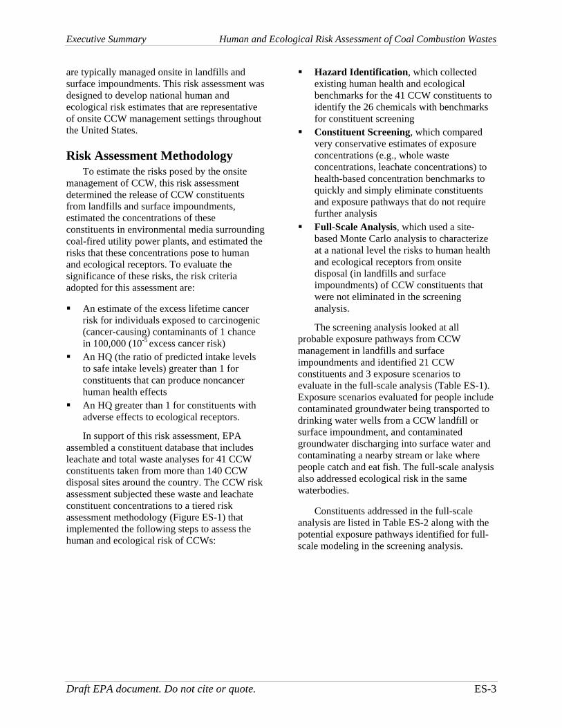
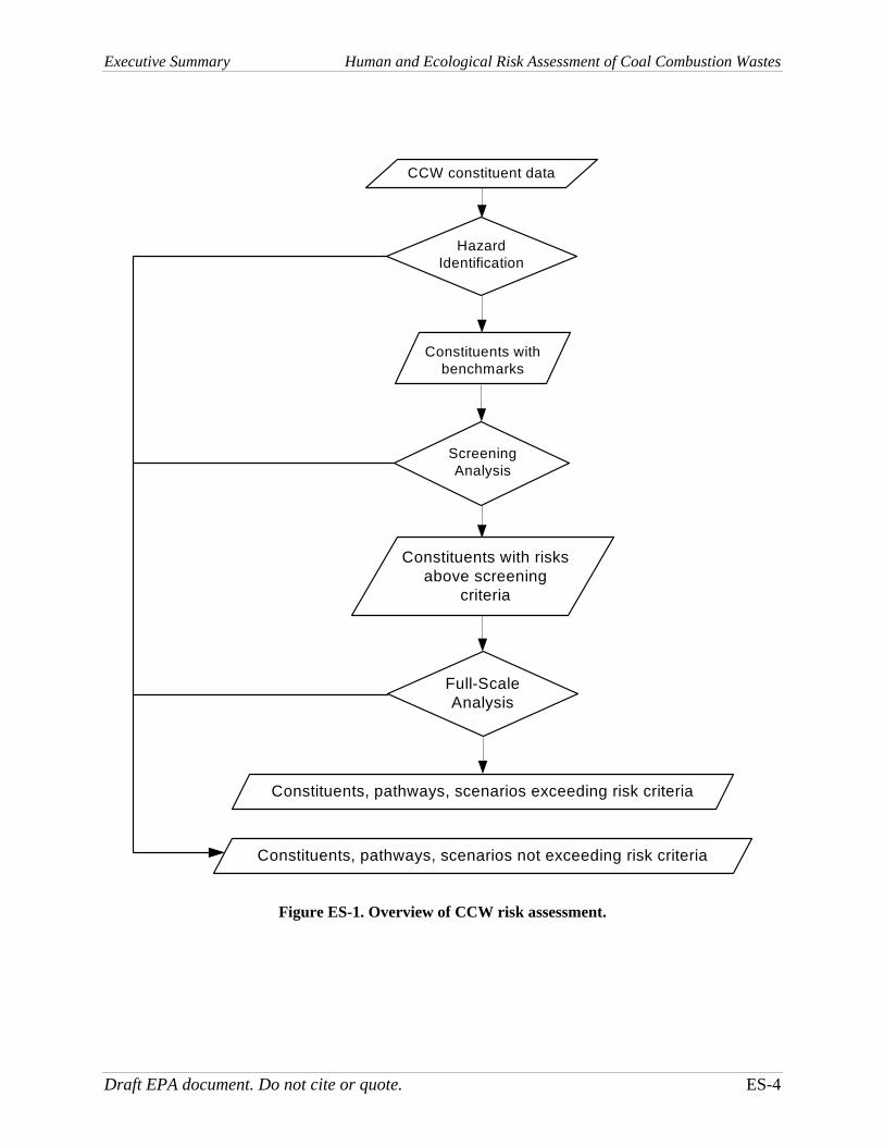
In support of this risk assessment, EPA assembled a constituent database that includes leachate and total waste analyses for 41 CCW constituents taken from more than 140 CCW disposal sites around the country. The CCW risk assessment subjected these waste and leachate constituent concentrations to a tiered risk assessment methodology (Figure ES-1) that implemented the following steps to assess the human and ecological risk of CCWs:
Hazard Identification, which collected existing human health and ecological benchmarks for the 41 CCW constituents to identify the 26 chemicals with benchmarks for constituent screening
Constituent Screening, which compared very conservative estimates of exposure concentrations (e.g., whole waste concentrations, leachate concentrations) to health-based concentration benchmarks to quickly and simply eliminate constituents and exposure pathways that do not require further analysis
Full-Scale Analysis, which used a site-based Monte Carlo analysis to characterize at a national level the risks to human health and ecological receptors from onsite disposal (in landfills and surface impoundments) of CCW constituents that were not eliminated in the screening analysis.
The screening analysis looked at all probable exposure pathways from CCW management in landfills and surface impoundments and identified 21 CCW constituents and 3 exposure scenarios to evaluate in the full-scale analysis (Table ES-1). Exposure scenarios evaluated for people include contaminated groundwater being transported to drinking water wells from a CCW landfill or surface impoundment, and contaminated groundwater discharging into surface water and contaminating a nearby stream or lake where people catch and eat fish. The full-scale analysis also addressed ecological risk in the same waterbodies.
Constituents addressed in the full-scale analysis are listed in Table ES-2 along with the potential exposure pathways identified for full-scale modeling in the screening analysis.
Executive Summary Human and Ecological Risk Assessment of Coal Combustion Wastes
Draft EPA document. Do not cite or quote. ES-4
CCW constituent data
Hazard Identification
Screening Analysis
Constituents with benchmarks
Constituents with risks above screening
criteria
Full-Scale Analysis
Constituents, pathways, scenarios exceeding risk criteria
Constituents, pathways, scenarios not exceeding risk criteria
Figure ES-1. Overview of CCW risk assessment.

Executive Summary Human and Ecological Risk Assessment of Coal Combustion Wastes
Draft EPA document. Do not cite or quote. ES-5
Table ES-1. Sources, Releases, Exposure Pathways, and Receptors Evaluated in the CCW Risk Assessment
Release Mechanism Exposure Pathway Exposure Mechanism Receptor Typea
Screening Result
Landfills
Groundwater-to-drinking-water
Residential well Resident Full-scale analysis
Leaching
Groundwater-to-surface-water
Stream or lake, uptake by fish; contact with water, sediments
Recreational fisher; aquatic ecosystems
Full-scale analysis
Overland transport to surface water
Stream or lake, uptake by fish; contact with water, sediments
Recreational fisher; aquatic ecosystems
Below screening criteria
Water erosion
Overland transport to soil
Soil ingestion; uptake from soil by plants, beef, dairy
Subsistence farmer; terrestrial ecosystems
Below screening criteriab
Soil deposition Soil ingestion; uptake from soil by plants, beef, dairy
Subsistence farmer; terrestrial ecosystems
Below screening criteria
Wind erosion
Fugitive dust Inhalation Resident Below screening criteria
Surface impoundments
Groundwater-to-drinking water
Residential well Resident Full-scale analysis
Leaching
Groundwater-to-surface water
Stream or lake, uptake by fish; contact with water, sediments
Recreational fisher; ecological receptors
Full-scale analysis
a Human receptor types include adults and children. b Except boron for plant toxicity. Also, damage cases indicate soil risks from selenium to terrestrial amphibians
(Carlson and Adriano, 1993; Hopkins et al., 2006).

Executive Summary Human and Ecological Risk Assessment of Coal Combustion Wastes
Draft EPA document. Do not cite or quote. ES-6
Table ES-2. Screening Analysis Results: CCW Constituents Selected for Full-Scale Analysisa
Human Health - Drinking Water
Human Health - Surface Waterb
Ecological Risk - Surface Water
Constituent LF SI LF SI LF SI
Arsenic • • • • • •
Boron • • • •
Cadmium • • • • • •
Lead • • • •
Selenium • • • • • •
Thallium • nd • nd • nd
Aluminum • •
Antimony • nd nd nd
Barium • •
Cobalt na • na na •
Molybdenum • •
Nitrate/Nitrite • •
Chromium • • • •
Fluoride • •
Manganese •
Vanadium • • • •
Beryllium •
Copper • •
Nickel • •
Silver • •
Zinc •
LF = landfill. SI = surface impoundment nd = nondetect—results are inconclusive because all analyses are nondetects. na = not available—data were not available for cobalt in CCW landfill leachate. a A mark in a cell indicates that the constituent was above the screening criteria for the indicated pathway and
WMU type. Blank cells indicate that the constituent was below the screening criteria for a particular pathway/WMU combination. Risk screening was based on 90th percentile risk concentrations and no attenuation.
b Fish consumption pathway.

Executive Summary Human and Ecological Risk Assessment of Coal Combustion Wastes
Draft EPA document. Do not cite or quote. ES-7
The full-scale analysis was designed to characterize waste management scenarios based on two waste management options (disposal of CCW onsite in landfills and in surface impoundments). The risk assessment was also used to characterize waste management scenarios based on three liner types (unlined units, clay-lined units, and composite-lined units) and three waste types, as follows:
Conventional CCW (ash and FGD sludge), which includes fly ash, bottom ash, boiler slag, and FGD sludge
Codisposed CCWs and coal refuse,3 which are more acidic than conventional CCWs due to sulfide minerals in the coal refuse
FBC wastes, which include fly ash and bed ash, and which tend to be more alkaline than conventional CCW because of the limestone mixed in during fluidized bed combustion.
These three waste types and the two waste management options provide a good representation of CCW disposal practices and waste chemistry conditions that affect the release of CCW constituents from WMUs.4,5
The full-scale analysis was implemented using a site-based probabilistic approach that produces a distribution of risks or hazards for each receptor by allowing the values of some of the parameters in the analysis to vary. This approach is ideal for this risk assessment because there are many CCW facilities across the United States, and a site-based approach can capture both the variability in waste management practices at these facilities and the differences in their environmental settings (e.g., hydrogeology, climate, hydrology). This
3 Coal refuse is the waste coal produced from coal
handling and preparation operations. 4 Conventional CCW and codisposed CCW and coal
refuse were modeled in landfills and surface impoundments and are the focus of the overall analysis. FBC wastes were treated separately because of limited data on FBC waste management units.
5 Although different waste chemistries required the separate modeling of conventional CCW and CCW codisposed with coal refuse, the results were combined in this analysis to give an overall picture of the risks from CCW management,
probabilistic approach was implemented through the following steps:
1. Characterize the CCW constituents and waste chemistry, along with the WMUs in which each waste stream may be managed (i.e., the size and liner status of CCW landfills and surface impoundments)
2. Characterize the environmental settings for the sites where CCW landfills and surface impoundments are located (i.e., locations of coal-fired power plants)
3. Identify how contaminants are released from a WMU (i.e., leaching) and transported to human and ecological receptors (i.e., via groundwater and surface water)
4. Predict the fate, transport, and concentration of constituents in groundwater and surface water once they are released to groundwater from the WMUs and travel to receptors at each site
5. Quantify the potential exposure of human and ecological receptors to the contaminant in the environment
6. Estimate the potential risk to each receptor from the exposure and characterize this risk in terms of exposure pathways and health effects.
Based on this approach, we characterized the potential risks associated with the waste disposal scenarios and exposure pathways, including the uncertainties associated with the analysis results.
Results and Conclusions Risks from clay-lined units are lower than
those from unlined units, but 90th percentile risks are still well above the risk criteria for arsenic and thallium for landfills and arsenic, boron, and molybdenum for surface impoundments. Composite liners, as modeled in this assessment, effectively reduce risks from all constituents to below the risk criteria for both landfills and surface impoundments. Although it is likely that today, most new landfills have some type of liner (based on more recent data that were not incorporated into this assessment),

Executive Summary Human and Ecological Risk Assessment of Coal Combustion Wastes
Draft EPA document. Do not cite or quote. ES-8
it is not known how many unlined units continue to operate in the United States.
Recent data from a joint DOE/EPA survey suggests that more facilities are lined today than were in the 1995 data set on which this risk assessment is based. This suggests that the risks from CCW may be lower than the results presented in this report, although the older, unlined WMUs represented in this risk assessment may continue to pose potential risks to human health and the environment if they are closed with wastes in place.
The CCW risk assessment results at the 90th percentile suggest that the management of CCW in landfills and surface impoundments as observed in 1995 for unlined and clay-lined units results in risks greater than the risk criteria of 10-5 for excess cancer risk to humans or an HQ greater than 1 for noncancer effects to both human and ecological receptors. Key risk findings include the following:
90th and 50th percentile risks for composite-lined units were consistently well below a cancer risk of 10-5 and an HQ of 1 for all constituents, waste management scenarios, and exposure pathways modeled in the CCW risk assessment.
For humans exposed via the groundwater-to-drinking-water pathway (see Figures ES-2 and ES-3), arsenic and thallium show risks to human health above the risk criteria for unlined and clay-lined CCW landfills. Arsenic poses a 90th percentile cancer risk of 5x10⁻⁴ for unlined units and 2x10⁻⁴ for clay-lined units; thallium shows a 90th percentile HQ above 1 for unlined units only. As shown in Figure ES-3, 50th percentile results are at or below risk criteria for all constituents.
Risks are higher for surface impoundments for the groundwater-to-drinking-water pathway, with a 90th-percentile arsenic cancer risk of 9x10⁻³ for unlined units and 3x10⁻³ for clay-lined units. For unlined units, 5 additional constituents have noncancer HQs ranging from 3 to 4 for the 90th percentile, including boron, lead, cadmium,
cobalt, and molybdenum. Two constituents (boron and molybdenum) have 90th percentile HQs greater than 1 (2 and 3, respectively) for clay-lined surface impoundments. The 50th percentile results are approximately 10-fold greater than the 10-5 cancer risk level for arsenic in unlined (3x10⁻⁴) and clay-lined (9x10⁻⁵) surface impoundments.
For humans exposed via the groundwater-to-surface-water (fish consumption) pathway, selenium (HQ = 2) and arsenic (cancer risk = 2x10⁻⁵) show 90th percentile risks for unlined surface impoundments slightly above the risk criteria. All other waste management scenarios and all 50th percentile results show risks at or below the risk criteria for the fish consumption pathway.
Waste type has little effect on landfill risk results, but surface impoundment risks are higher for codisposed CCW and coal refuse than for conventional CCW.
Higher risks for surface impoundments than landfills are likely due to a combination of higher waste leachate concentrations, a higher proportion of unlined units, and a higher hydraulic head from impounded liquid waste. This is consistent with damage cases reporting wet handling as a factor that can increase risks from CCW management.
For ecological receptors exposed via surface water, the 90th percentile risks for landfills exceed an HQ of 1 for boron and lead. For surface impoundments, risks for the 90th percentile for 6 constituents (boron, lead, arsenic, selenium, cobalt, and barium) exceed an HQ of 1, with boron showing the highest risks (HQ over 2,000). The exceedances for boron and selenium are consistent with reported ecological damage cases, which include impacts to waterbodies through the groundwater-to-surface-water pathway (e.g., Carlson and Adriano, 1993; U.S. EPA, 2007). Only boron exceeds the ecological risk criterion for surface water at the 50th percentile, with an HQ of 4.

Executive Summary Human and Ecological Risk Assessment of Coal Combustion Wastes
Draft EPA document. Do not cite or quote. ES-9
CCW Landfills
1.E-06 1.E-05 1.E-04 1.E-03 1.E-02
Arsenic (cancer)
Cancer risk = 10-5
1E-06 1E-05 0.0001 0.001 0.01 0.1 1 10 100 1000
Nitrate/Nitrate (MCL)
Selenium
Boron
Cadmium
Lead (MCL)
Molybdenum
Antimony
Thallium
90th Percentile Human Health Riskcomposite-lined units clay-lined units unlined units all units combined
HQ = 1
CCW Surface Impoundments
1.E-09 1.E-08 1.E-07 1.E-06 1.E-05 1.E-04 1.E-03 1.E-02
Arsenic (cancer)
Cancer risk = 10-5
0.0001 0.001 0.01 0.1 1 10 100 1000
Nitrate (MCL)
Selenium
Boron
Lead (MCL)
Cadmium
Cobalt
Molybdenum
90th Percentile Human Health Risk
composite-lined units clay-lined units unlined units all units combined
HQ = 1
A cancer risk of 10-5 or an HQ of 1 are the risk criteria for this analysis.
Results for “all units combined” are results across all liner types (unlined, clay-lined, composite-lined). Note: When the composite liner bar does not appear on the chart, the 90th percentile risk index
is below the minimum shown on the x-axis.
Figure ES-2. Full-scale 90th percentile risk results for the groundwater-to-drinking-water pathway.

Executive Summary Human and Ecological Risk Assessment of Coal Combustion Wastes
Draft EPA document. Do not cite or quote. ES-10
CCW Landfills
1.E-11 1.E-10 1.E-09 1.E-08 1.E-07 1.E-06 1.E-05 1.E-04
Arsenic (cancer)
Cancer risk = 10-5
0.000001 0.00001 0.0001 0.001 0.01 0.1 1 10
Lead (MCL)
Nitrate/Nitrate (MCL)
Boron
Cadmium
Selenium
Molybdenum
Antimony
Thallium
50th Percentile Human Health Riskcomposite-lined units clay-lined units unlined units all units combined
HQ= 1
CCW Surface Impoundments
1.E-09 1.E-08 1.E-07 1.E-06 1.E-05 1.E-04 1.E-03
Arsenic (cancer)
Cancer risk = 10-5
0.0001 0.001 0.01 0.1 1 10 100
Cobalt
Nitrate (MCL)
Lead (MCL)
Cadmium
Selenium
Boron
Molybdenum
50th Percentile Human Health Risk
composite-lined units clay-lined units unlined units all units combined
HQ = 1
A cancer risk of 10-5 or an HQ of 1 are the risk criteria for this analysis.
Results for “all units combined” are results across all liner types (unlined, clay-lined, composite-lined). Note: When the composite liner bar does not appear on the chart, the 50th percentile risk index
is below the minimum shown on the x-axis.
Figure ES-3. Full-scale 50th percentile risk results for the groundwater-to-drinking-water pathway.

Executive Summary Human and Ecological Risk Assessment of Coal Combustion Wastes
Draft EPA document. Do not cite or quote. ES-11
For ecological receptors exposed via sediment, 90th percentile risks for lead, arsenic, and cadmium exceeded a HQ of 1 for both landfills (HQs from 2 to 20) and surface impoundments (HQs from 20 to200) probably because these constituents strongly sorb to sediments. No constituents exceed the ecological risk criterion for sediments at the 50th percentile.
Sensitivity analysis results indicate that for more than 75 percent of the scenarios evaluated, the risk assessment model was most sensitive to parameters related to groundwater flow and transport, including WMU infiltration rate, leachate concentration, and aquifer hydraulic conductivity and gradient. For the groundwater-to-surface water pathway, another sensitive parameter is the flowrate of the waterbody into which the contaminated groundwater is discharging. For strongly sorbing contaminants (such as lead and cadmium), variables related to sorption and travel time (adsorption coefficient, depth to groundwater, receptor well distance) are also important.
The multiple uncertainties associated with the CCW risk assessment include scenario uncertainty (i.e., uncertainty about the environmental setting around the plant), uncertainty in human exposure factors (such as exposure duration, body weight, and intake rates), uncertainty in human and ecological toxicity factors and potential cumulative risks, and uncertainty in estimates of fate and transport of waste constituents in the environment. Scenario uncertainty has been minimized by basing the risk assessment on conditions around existing coal-fired power plants around the United States, as observed in 1995. Uncertainty in environmental setting parameters has been incorporated into the risk assessment by varying these inputs within reasonable ranges when the exact value is not known. Uncertainty in human exposure factors has also been addressed through the use of national distributions.
Some uncertainties not addressed explicitly in the risk assessment have been addressed through comparisons with other studies and data sources, as described below:
Appropriateness of CCW leachate data. Although porewater data were available and used for CCW surface impoundments,
available data for landfills were mainly Toxicity Characteristic Leaching Procedure (TCLP) analyses, which may not be representative of actual CCW leachate. Comparisons with recent (2006) studies of coal ash leaching processes show very good agreement for arsenic. However, although the selenium CCW data are within the range of the 2006 data, some of the higher concentrations in the 2006 data are not represented by the TCLP data. This suggests that selenium risks may be underestimated, which is consistent with selenium as a cause for CCW damage cases.
Limited CCW leachate data. Because of a high proportion of nondetect values6 and a limited number of measurements, mercury could not be addressed in the CCW risk assessment for landfills or surface impoundments, and antimony and thallium could not be assessed in surface impoundments. Mercury levels in leachate were measured in EPA’s 2006 leaching study and suggest a limited concern for mercury for the CCW leachates investigated, but additional work is needed to extend these results to all CCW disposal facilities.
Clean Air Interstate Rule (CAIR) and Clean Air Mercury Rule (CAMR) impacts. While CAIR and CAMR will reduce air emissions of mercury and other metals from coal-fired power plants, mercury and other more volatile metals will be transferred from the flue gas to fly ash and other air pollution control residues, including the sludge from wet scrubbers. EPA is conducting research on how much total mercury will increase in CCW from the use of mercury controls, as well as how the leachability of mercury and other metals will be impacted. Preliminary results suggest that the impacts on mercury leaching will depend on the mercury control process.
Arsenic speciation. The current model does not speciate metals during subsurface
6 Nondetect values are measurements where the
concentration of a constituent is below the level that the analytical instrument can detect. The actual level could range from zero to just below the detection limit. Nondetects for constituents other than mercury were modeled at one-half the detection limit for this risk analysis.

Executive Summary Human and Ecological Risk Assessment of Coal Combustion Wastes
Draft EPA document. Do not cite or quote. ES-12
transport. Damage cases and other studies suggest that arsenic readily converts from arsenic III in CCW leachate to the less mobile arsenic V in soil and groundwater. However, model runs conducted for both species suggest that the difference in risk between the two species is only about a factor of 2 at the 90th percentile risk level, which is not enough to bring arsenic risks below the risk criteria.
Uncertainties that EPA does not have enough data at this time to evaluate with respect to CCW risk results include the following:
Well distance. Nearest well distances were taken from a survey of municipal solid waste (MSW) landfills because data were not available from CCW sites. EPA believes that this is a protective assumption because MSW landfills generally tend to be in more populated areas, but there are little data available to test this hypothesis.
Liner performance. Liner design and performance for CCW WMUs were based on data and assumptions EPA developed to be appropriate for municipal and nonhazardous industrial waste landfills. EPA believes that CCW landfills should have similar performance characteristics, but does not have quantitative data on CCW WMU liners to verify that.
Data gaps for ecological receptors. Data were insufficient to develop screening levels
and quantitative risk estimates for terrestrial amphibians, but EPA acknowledges that damage cases indicate risk to terrestrial amphibians through exposure to selenium (e.g., Hopkins et al., 2006).
Ecosystems and receptors at risk. Certain critical assessment endpoints were not evaluated in this analysis, including impacts on managed lands, critical habitats, and threatened and endangered species. These would be addressed through more site-specific studies on the proximity of these areas and species to CCW disposal units.
Synergistic and additive risk. The impact of exposures to multiple contaminants on human and ecological risks was not evaluated in this analysis. EPA recognizes that a single-constituent analysis may underestimate risks associated with multiple chemical exposures. The risk assessment also does not add risks across pathways (i.e., risks from drinking water and fish consumption), but EPA does not think that doing so would change the results markedly because the constituents of concern differ between pathways.
EPA recognizes that uncertainties in mercury levels in CCW leachate, both with and without the CAIR/CAMR mercury controls, represent a potentially significant gap in our knowledge of CCW risks.

Section 1.0 Introduction
Draft EPA document. Do not cite or quote. 1-1
1.0 Introduction
1.1 Background
The U.S. Environmental Protection Agency (EPA) has evaluated the human health and environmental risks associated with coal combustion waste (CCW) management practices, including disposal in landfills and surface impoundments. In May 2000, EPA determined that regulation as hazardous wastes under Subtitle C of the Resource Conservation and Recovery Act (RCRA) was not warranted for certain CCWs, but that regulation as nonhazardous wastes under RCRA Subtitle D was appropriate. However, EPA did not specify regulatory options at that time. This risk assessment was designed and implemented to help EPA identify and quantify human health and ecological risks that may be associated with current management practices for high-volume CCWs. These wastes are fly ash, bottom ash, boiler slag, and flue gas desulfurization (FGD) sludge, along with wastes from fluidized-bed combustion (FBC) units and CCWs codisposed with coal refuse. This risk assessment will help EPA develop CCW management options for these high-volume waste streams. Details on EPA’s CCW work to date can be found at http://www.epa.gov/epaoswer/other/fossil/index.htm.
Note that the full-scale risk assessment described in this report was mostly conducted in 2003, meaning that the data collection efforts to support the risk assessment were based on the best information available to EPA at that time. As a result, more recent Agency efforts to characterize CCW wastes and management practices, such as the joint EPA and U.S. Department of Energy (DOE) survey of CCW waste management units (WMUs) (U.S. DOE, 2006) and EPA’s recent study of CCW chemistries and leaching behavior (U.S. EPA, 2006), were not considered in the main analysis phase of this risk assessment. However, these more recent efforts are discussed as part of the risk characterization, and EPA is currently evaluating how to best incorporate and address the results and findings of these studies in future efforts to address CCW management practices.
The Agency is making the risk analysis document available in the Docket1 to allow interested parties to submit comments on the analytical methodology, data, and assumptions used in the analysis and to submit additional information for the Agency to consider. In addition, the risk assessment will undergo independent scientific peer review by experts outside EPA following closure of the public comment period. Public comments will be made available to the peer reviewers for their consideration during the review process. The peer review will focus on technical aspects of the analysis, including the construction and implementation of the Monte Carlo analysis, the selection of models to estimate the release of constituents found in CCW from landfills and surface impoundments and their subsequent fate and transport in the environment, and the characterization of risks resulting from potential exposures to human and ecological receptors. As appropriate, EPA will update this analysis based on both public and peer-review comments.
1 Available at http:www.regulations.gov; docket number EPA-HQ-RCRA-2006-0796.

Section 1.0 Introduction
Draft EPA document. Do not cite or quote. 1-2
1.2 Purpose and Scope of the Risk Assessment
The purpose of this risk assessment is to identify CCW constituents, waste types, exposure pathways, and receptors that may produce risks to human and ecological health, and to provide information about those scenarios that EPA can use to develop management options for CCW management.
The scope of this risk assessment is utility CCWs managed onsite at utility power plants. EPA’s Report to Congress: Wastes from the Combustion of Fossil Fuels (U.S. EPA, 1999a) reports that there are 440 coal-fired utility power plants in the United States. Although these plants are concentrated in the East, they are found in nearly every state, with facility settings ranging from urban to rural. The large volumes of waste generated by these plants are typically managed onsite in landfills and surface impoundments. This risk assessment was designed to develop national human and ecological risk estimates that are representative of onsite CCW management settings throughout the United States.
1.3 Overview of Risk Assessment Methodology
To estimate the risks posed by the onsite management of CCW, this risk assessment estimated the release of CCW constituents from landfills and surface impoundments, the concentrations of these constituents in environmental media surrounding coal-fired utility power plants, and the risks that these concentrations pose to human and ecological receptors.
The size, design, and locations of the onsite CCW landfills and surface impoundments modeled in this risk assessment are based on data from a national survey of utility CCW disposal conducted by the Electric Power Research Institute (EPRI) in 1995 (EPRI, 1997). Data from this survey on facility area, volume, and liner characteristics were used in the CCW risk assessment because they were the most recent and complete data set available at the time the risk assessment was conducted (2003). However, as shown in Table 1-1, the EPA/DOE study conducted since then (U.S. DOE, 2006) shows a much higher proportion of lined facilities than do the 1995 EPRI data.
Table 1-1. Liner Prevalence in EPRI and DOE Surveys
Liner Type Landfills Surface
Impoundments 1995 EPRI Surveya – 181 facilities Unlined 40% 68% Lined (compacted clay or composite [clay and synthetic]) 60% 32%
2004 DOE Surveyb – 56 Facilities Unlined 3% 0% Lined (compacted clay or composite [clay and synthetic]) 97% 100% a EPRI (1997) b U.S. DOE (2006)

Section 1.0 Introduction
Draft EPA document. Do not cite or quote. 1-3
The releases, and hence media concentrations and risk estimates, are based on leaching to groundwater, wind and water erosion, and overland transport. This analysis does not address direct releases to surface water, which are permitted under the National Pollutant Discharge Elimination System (NPDES) of the Clean Water Act. Thus, the estimated media concentrations and risks do not take into account contributions from NPDES-permitted releases, including discharges due to flooding or heavy rainfall.
To evaluate the significance of the estimated risks, the risk criteria adopted for this assessment are
An estimate of the excess lifetime cancer risk for individuals exposed to carcinogenic (cancer-causing) contaminants of 1 chance in 100,000 (10-5 excess cancer risk)2
A measure of safe intake levels to predicted intake levels, a hazard quotient (HQ) greater than 1 for constituents that can produce noncancer human health effects (an HQ of 1 is defined as the ratio of a potential exposure to a constituent to the highest exposure level at which no adverse health effects are likely to occur)
An HQ greater than 1 for constituents with adverse effects to ecological receptors.
In 1998, EPA conducted a risk assessment for fossil fuel combustion wastes (which include CCWs) to support the May 2000 RCRA regulatory determination (U.S. EPA, 1998a,b). Since then, EPA has added to the waste constituent database that was used in that effort, expanding the number of leachate and total waste analyses for 41 CCW constituents. The CCW risk assessment subjected these waste and leachate constituent concentrations to the tiered risk assessment methodology illustrated in Figure 1-1. This methodology implemented the following steps to assess the human and ecological risk of CCWs:
Hazard Identification, which collected existing human health and ecological benchmarks for the CCW constituents. Only constituents with benchmarks move on to the next step, constituent screening.
Constituent Screening, which compared very conservative estimates of exposure concentrations (e.g., whole waste concentrations, leaching concentrations) to health-based concentration benchmarks to quickly and simply identify constituents and exposure pathways with risks below the screening criteria.
Full-Scale Analysis, which characterized at a national level the human health and ecological risks for constituents in CCW disposed onsite in landfills and surface impoundments using a site-based Monte Carlo risk analysis.
This document focuses on the full-scale Monte Carlo analysis. Constituent screening results are also presented as part of the problem formulation discussion, along with a summary of the screening methodology.3
2 The typical cancer risk range used by the Office of Solid Waste and Emergency Response is 10-4 to 10-6. In
hazardous waste listings, the point of departure for listing a waste is 10-5. 3 Details on the CCW constituent screening analysis can be found in U.S. EPA (2002a).

Section 1.0 Introduction
Draft EPA document. Do not cite or quote. 1-4
CCW constituent data
Hazard Identification
Screening Analysis
Constituents with benchmarks
Constituents with risks above
criteria
Full-Scale Analysis
Constituents, pathways, scenarios exceeding risk criteria
Constituents, pathways, scenarios not exceeding risk criteria
Constituents with no benchmarks
Constituents with no risks above
criteria
Figure 1-1. Overview of coal combustion waste risk assessment.

Section 1.0 Introduction
Draft EPA document. Do not cite or quote. 1-5
1.3.1 Waste Management Scenarios
The full-scale analysis was designed to characterize waste management scenarios based on two waste management options (disposal of CCW onsite in landfills and in surface impoundments) and three waste types, as follows:
Conventional CCW, which includes fly ash, bottom ash, boiler slag, and FGD sludge
Codisposed CCWs and coal refuse,4 which are more acidic than conventional CCWs due to sulfide minerals in the mill rejects
FBC wastes, which include fly ash and the fluidized bed ash, and which tend to be more alkaline than conventional CCW because of the limestone mixed in during fluidized bed combustion.
Conventional CCW and codisposed CCW and coal refuse are typically disposed of in landfills and surface impoundments that can be lined with clay or composite liners. FBC wastes are only disposed of in landfills in the United States; therefore, surface impoundment disposal was not modeled for FBC waste.
These three waste types, two waste management options, and three liner conditions (unlined, clay-lined, composite-lined) modeled in this analysis provide a good representation of CCW disposal practices and waste chemistry conditions that affect the release of CCW constituents from WMUs.
1.3.2 Approach
The full-scale analysis was implemented using a site-based probabilistic approach that produces a distribution of risks or hazard for each receptor by allowing the values of some of the parameters in the analysis to vary. This approach is ideal for this risk assessment because there are many CCW facilities across the United States, and a site-based approach can capture both the variability in waste management practices at these facilities and the differences in their environmental settings (e.g., hydrogeology, climate, hydrology). This probabilistic approach was implemented through seven primary steps:
Problem Formulation
1. Characterize the CCW constituents and waste chemistry, along with the size and liner status of the WMUs in which each waste stream may be managed
2. Characterize the environmental settings for the sites where CCW landfills and surface impoundments are located
4 Coal refuse is the waste coal produced from coal handling, crushing, and sizing operations, and tends to have a
high sulfur content and low pH from high amounts of sulfide minerals (like pyrite). In the CCW constituent database, codisposed coal refuse includes “combined ash and coal gob,” “combined ash and coal refuse,” and “combined bottom ash and pyrites.”

Section 1.0 Introduction
Draft EPA document. Do not cite or quote. 1-6
3. Identify scenarios under which contaminants are released from a WMU and transported to a human receptor
Analysis
4. Predict the fate and transport of constituents in the environment once they are released from the WMUs at each site
5. Quantify the exposure of human and ecological receptors to the contaminant in the environment and the risk associated with this exposure
Risk Characterization
6. Estimate the risk to receptors from the exposure and characterize this risk in terms of exposure pathways, health effects, and uncertainties
7. Identify the waste disposal scenarios and environmental conditions that pose risks to human health or the environment that are above the risk criteria. Evaluate risks at the 50th and 90th percentiles.
1.4 Document Organization
This document is organized into the following sections:
Section 2, Problem Formulation, describes how the framework for the full-scale analysis was developed, including identification of the waste constituents, exposure pathways, and receptors of concern; selection and characterization of waste management practices and sites to model; and development of the conceptual site models for the modeling effort.
Section 3, Analysis, describes the probabilistic modeling framework and the models and methods used to (1) estimate constituent releases from CCW landfills and surface impoundments (source models), (2) model constituent concentrations in the environmental media of concern (groundwater and surface water), (3) calculate exposure, and (4) estimate risk to human and ecological receptors.
Section 4, Risk Characterization, characterizes the human health and environmental risks posed by CCW, including (1) discussion of the methods used to account for variability and uncertainty and (2) identification of the scenarios and conditions that result in risks above the risk criteria. Results are presented as national estimates for CCW landfills and CCW surface impoundments, as well as by waste type and liner status. For risk exceedances, this section identifies the CCW constituents and pathways that exceed the risk criteria, along with any factors (such as liners or facility environmental setting) that might result in higher or lower risk levels. Finally, the risk characterization evaluates the risk results in light of more recent research on CCW waste management practices and the environmental behavior of CCW constituents.
Section 1.0 Introduction
Draft EPA document. Do not cite or quote. 1-7
The first three appendices provide detailed information on how wastes, WMUs, and settings were characterized for the risk assessment. Appendix A describes the chemical characteristics of the wastes disposed in the WMUs, including the CCW leachate concentration distributions used. Appendix B describes how EPA characterized the WMUs (landfills and surface impoundments), including surface area, capacities, geometry, and liner status. Appendix C presents the methodologies and data used to characterize the environmental setting at each CCW site, including delineating the site layout and determining the environmental setting (e.g., meteorology, climate, soils, aquifers, and waterbodies).
The remaining appendices provide detailed information on the specific models and data used to calculate risk, including the nonlinear sorption isotherms (Appendix D), the surface water fate and transport and intake equations (Appendix E), the exposure factors (Appendix F), and benchmarks for human health (Appendix G) and ecological risk (Appendix H).


Section 2.0 Problem Formulation
Draft EPA document. Do not cite or quote. 2-1
2.0 Problem Formulation The full-scale CCW risk assessment is intended to evaluate, at a national level, risk to
individuals who live near WMUs used for CCW disposal. This section describes how the conceptual framework for the full-scale risk assessment was developed, including
Constituent selection and screening to identify the CCW constituents, exposure pathways, and receptors to address in this analysis (Section 2.1.1)
Location and characterization of the CCW landfills and surface impoundments to be modeled as the sources of CCW contaminants in the site-based analysis (Section 2.1.2)
The conceptual site model used to represent CCW disposal facilities (Section 2.2)
The general modeling approach and scope (Section 2.3), including data collection, fate and transport modeling to estimate exposure point concentrations, exposure assessment, and the calculation of risks to human and environmental receptors.
2.1 Source Characterization
The main technical aspects of the CCW risk assessment were completed in 2003, and the waste management scenarios modeled in this assessment are based on the best data on industry operations and waste management practices that were available at that time. These data sources include a 1995 industry survey on CCW management practices (the EPRI comanagement survey [EPRI, 1997]) and data collected from a variety of sources before the 2003 risk assessment (e.g., EPA’s CCW constituent database). Since 2003, DOE and EPA have completed a survey to characterize CCW waste disposal practices from 1994 to 2004, with a focus on new facilities or facility expansions completed within that same time frame (U.S. DOE, 2006). Although these newer data were not available when this risk assessment was conducted, they are discussed in the risk characterization (Section 4) as an uncertainty with respect to how well the risk assessment represents current WMU liner conditions.
This risk assessment provides a national characterization of waste management scenarios for wastes generated by coal-fired utility power plants. The sources modeled in these scenarios are onsite landfills and surface impoundments, which are the primary means by which CCW is managed in the United States. The characterization of these sources, in terms of their physical dimensions, operating parameters, location, environmental settings, and waste characteristics, is fundamental to the construction of scenarios for modeling. This section describes how the coal combustion waste streams and management practices were characterized (based on the above data sources) and screened to develop the waste disposal scenarios modeled in the full-scale analysis.

Section 2.0 Problem Formulation
Draft EPA document. Do not cite or quote. 2-2
2.1.1 Identification of Waste Types, Constituents, and Exposure Pathways
To identify the CCW constituents and exposure pathways to be addressed in this risk assessment, we relied on a database of CCW analyses that EPA had assembled over the past several years to characterize whole waste and waste leachate from CCW disposal sites across the country (see Appendix A). The 2003 CCW constituent database includes all of the CCW characterization data used by EPA in its previous risk assessments, supplemented with additional data collected from public comments, data from EPA Regions and state regulatory agencies, industry submittals, and literature searches up to 2003.
The CCW constituent database represents a significant improvement in the quantity and scope of waste characterization data available from the 1998 EPA risk assessment of CCWs (U.S. EPA, 1998a,b). For example, the constituent data set used for the previous risk assessments (U.S. EPA, 1999a) covered approximately 50 CCW generation and/or disposal sites. With the addition of the supplemental data, the 2003 CCW constituent database covers approximately 140 waste disposal sites.1 The 2003 database also has broader coverage of the major ion concentrations of CCW leachate (e.g., calcium, sulfate, pH).
2.1.1.1 Waste Types
Comments received by EPA on the previous CCW risk assessment pointed out that the analysis did not adequately consider the impacts of CCW leachate on the geochemistry and mobility of metal constituents in the subsurface. Commenters stated that given the large size of the WMUs and the generally alkaline nature of CCW leachate, it is likely that the leachate affects the geochemistry of the soil and aquifers underlying CCW disposal facilities, which can impact the migration of metals in the subsurface.
To address this concern, EPA statistically evaluated major ion porewater data from the CCW constituent database for the waste streams shown in Table 2-1. Based on this analysis and prevalent comanagement practices, EPA grouped the waste streams into three statistically distinct categories: conventional CCW (ash and FGD sludge) (moderate to high pH); codisposed CCW and coal refuse (low pH); and FBC waste (high pH). As shown in Table 2-1, each of these waste types includes several waste streams that are usually codisposed in landfills or surface impoundments.
Along with the type of WMU (landfill or surface impoundment), the three waste types in Table 2-1 define the basic modeling scenarios to be addressed in the full-scale analysis. To characterize these waste types, the CCW constituent database was queried by waste type to develop the waste concentration data for the constituents and the major ion and pH conditions used to develop waste-type-specific metal sorption isotherms (see Appendix D for a more extensive discussion of the development of CCW waste chemistries and metal sorption isotherms).
1 Although EPA believes that the 140 waste disposal sites do represent the national variability in CCW
characteristics, they are not the same sites as in the EPRI survey. During full-scale modeling, data from the CCW constituent database were assigned to each EPRI site based on the waste types reported in the EPRI survey data.

Section 2.0 Problem Formulation
Draft EPA document. Do not cite or quote. 2-3
Table 2-1. Waste Streams in CCW Constituent Database
Number of Sites by Waste Typea
Waste Type Waste Streams
Landfill Leachate
Surface Impoundment
Porewater Total
Wasteb Conventional CCW 97 13 62
Ash (not otherwise specified) 43 0 30 Fly ash 61 2 33 Bottom ash and slag 24 3 23 Combined fly and bottom ash 7 4 4 FGD sludge 4 6 5
Codisposed Ash & Coal Refuse 9 5 1 FBC Waste 58 0 54
Ash (not otherwise specified) 18 0 10 Fly ash 33 0 32 Bottom and bed ash 26 0 25 Combined fly & bottom ash 20 0 22
a Number of sites by waste type from leachate, porewater, and whole waste data tables in the 2003 CCW constituent database.
b Whole waste concentration data.
2.1.1.2 Constituents and Pathways
The CCW constituent database contains data on more than 40 constituents. During the hazard identification step of the CCW risk assessment, constituents of potential concern were identified from this list of constituents by searching EPA and other established sources for human health and ecological benchmarks (e.g., Agency for Toxic Substances and Disease Registry [ATSDR]; see U.S. EPA, 2002a, for a full list of sources). Table 2-2 shows the results of that search for each constituent. Benchmarks were found for 26 chemicals in the constituent database. Constituents without human health or ecological benchmarks were not addressed further in the risk analysis.2
To further narrow down the list of constituents, a screening analysis (U.S. EPA, 2002a) was conducted that compared very conservative estimates of exposure concentrations (e.g., whole waste concentrations, leaching concentrations) to health-based concentration benchmarks to quickly, simply, and safely identify constituents and exposure pathways with risks that clearly do not exceed the risk criteria so that these could be eliminated from further analysis. For example, leachate concentrations were compared directly to drinking water standards, which is equivalent to assuming that human receptors are drinking leachate. The technical background document for the CCW screening analysis (U.S. EPA, 2002a) provides further detail on the
2 The CCW constituents without benchmarks are limited to common elements, ions, and compounds (e.g., iron,
magnesium, phosphate, silicon, sulfate, sulfide, calcium, pH, potassium, sodium, carbon, sulfur) that were used to determine overall CCW chemistries modeled in the risk assessment (see Section 3). Although some of these chemicals or parameters (e.g., pH, sulfate, phosphate, chloride) can pose an ecological hazard if concentrations are high enough, they were not addressed in this risk assessment.

Section 2.0 Problem Formulation
Draft EPA document. Do not cite or quote. 2-4
Table 2-2. Toxicity Assessment of CCW Constituents
Constituent CAS ID HHBa EcoBb Constituent CAS ID HHBa EcoBb Metals Inorganic Anions Aluminum 7429-90-5 U U Chloride 16887-00-6 Antimony 7440-36-0 U U Cyanide 57-12-5 U Arsenic 7440-38-2 Uc U Fluoride 16984-48-8 U Barium 7440-39-3 U U Nitrate 14797-55-8 U Beryllium 7440-41-7 Ud U Nitrite 14797-65-0 U Boron 7440-42-8 U U Phosphate 14265-44-2 Cadmium 7440-43-9 Ud U Silicon 7631-86-9 Chromium 7440-47-3 Uc U Sulfate 14808-79-8 Cobalt 7440-48-4 U U Sulfide 18496-25-8 Copper 7440-50-8 Ue U Inorganic Cations Iron 7439-89-6 Ammonia 7664-41-7 U Lead 7439-92-1 Ue U Calcium 7440-70-2 Magnesium 7439-95-4 pH 12408-02-5 Manganese 7439-96-5 U Potassium 7440-09-7 Mercury 7439-97-6 U U Sodium 7440-23-5 Molybdenum 7439-98-7 U U Nonmetallic Elements Nickel 7440-02-0 U U Carbon 7440-44-0 Selenium 7782-49-2 U U Sulfur 7704-34-9 Silver 7440-22-4 U U Measurements Strontium 7440-24-6 U Total Dissolved Solids none Thallium 7440-28-0 U U Total Organic Carbon none Vanadium 7440-62-2 U U Dissolved Organic Carbon none Zinc 7440-66-6 U U a HHB = human health effect benchmark b EcoB = ecological benchmark c Known carcinogen (for chromium VI, inhalation only); although arsenic can act as both a carcinogen and a
noncarcinogen, the cancer risk exceeds the noncancer risk at any concentration, so we used the more protective cancer benchmark for human health throughout this assessment.
d Probable carcinogen e Safe Drinking Water Act Action Level only
screening analysis. As detailed there, the risks for all above-ground pathways analyzed (soil ingestion, inhalation, gardening, beef and dairy, and erosion and overland transport) for human receptors did not exceed the screening criteria for any constituent, so they were not considered any further in the risk assessment. The above-ground pathway risks for ecological receptors also did not exceed the screening criteria except for boron and selenium. Boron, which showed risks above the risk criterion in above-ground pathways due to plant toxicity in the CCW screening analysis, has been shown to be toxic to plants (Carlson and Adriano, 1993). Selenium has shown toxicity to terrestrial amphibians via above-ground pathways (Carlson and Adriano, 1993; Hopkins et al., 2006). Because the risks posed by these CCW constituents to ecological communities via above-ground pathways is well documented in damage cases and field studies (see above references and U.S. EPA, 2007), we did not believe that a full-scale above-ground

Section 2.0 Problem Formulation
Draft EPA document. Do not cite or quote. 2-5
pathway analysis was necessary to confirm this conclusion for two constituents. Thus, the full-scale risk assessment did not include any above-ground pathways, only groundwater pathways.
The groundwater-to-drinking-water and groundwater-to-surface-water pathways (human fish consumption and ecological risks) did show risks above the screening criteria for several CCW constituents in the screening analysis. Table 2-3 lists the 21 constituents that had 90th percentile screening analysis groundwater pathway risks greater than a cancer risk of 1 in 100,000 or a noncancer risk with an HQ greater than 1 for human health and 10 for ecological risk.3 Note that mercury was not addressed in the screening or full-scale analysis because of a very high proportion of nondetects in the CCW constituent database. Similarly, a high number of nondetects (or a very low number of measurements) prevented screening or full-scale analysis for antimony, thallium, and cobalt in surface impoundments. The uncertainties associated with these limited analytical results are discussed in Section 4.4.3.1.
Resources did not allow full-scale modeling to be conducted for all 21 constituents that had 90th percentile risks above the screening criteria. To reduce the number of constituents to be modeled, those constituents were ranked and divided into two groups to focus the full-scale analysis on the CCW constituents that were likely to pose relatively higher risks to human and ecological receptors. The ranking was based on the magnitude of the HQs and the number of HQs exceeding the screening criteria, and was used to select chemicals for full-scale modeling. Constituents with at least one human health HQ greater than 6 or with ecological HQs greater than 100 for both landfills and surface impoundments were modeled. Arsenic, with cancer risks greater than 1 in 1,000, exceeded the cancer risk criterion by a factor of 100 and was also modeled in the full-scale analysis. Constituents with no human health HQs greater than 6 and only one or no ecological HQs greater than 100 were not modeled, but were addressed in a separate analysis using results from the modeled constituents.
Table 2-3 shows the 21 constituents and which of these constituents exceeded the screening criteria and thus were modeled in the full-scale analysis. As shown, 12 constituents were subjected to the full-scale probabilistic risk assessment described in this document. Nine constituents did not exceed the screening criteria and were addressed using risk factors developed from comparing the screening and full-scale results for the modeled constituents, as described in Section 4.1.5 of this document.
2.1.2 Waste Management Scenarios
The full-scale CCW risk assessment models landfills and surface impoundments managing wastes onsite at coal-fired utility power plants. Because EPA selected a site-based modeling approach for the full-scale analysis, it was necessary to locate these disposal sites across the country to provide the spatial foundation for this analysis. It was also necessary to characterize CCW WMUs to define the scope for source modeling.
3 An HQ of 10 was used for screening ecological risks to account for conservatism of ecological benchmarks and
exposure estimates used in the screening analysis (see Section 4.4.3.4).

Section 2.0 Problem Formulation
Draft EPA document. Do not cite or quote. 2-6
Table 2-3. Screening Analysis Results: Selection and Prioritization of CCW Constituents for Further Analysisa
Human Health – Drinking Water
Human Health – Surface Waterb
Ecological Risk - Surface Water
Constituent
LF HQ (Cancer
Risk)
SI HQ (Cancer
Risk)
LF HQ (Cancer
Risk)
SI HQ (Cancer
Risk) LF HQ
SI HQ
Constituents Modeled in Full-scale Assessment Carcinogen Arsenicc (1.4x10⁻³) (1.8x10⁻²) (2.2x10⁻⁴) (1.7x10⁻⁵) 49 640 Noncarcinogens Boron 4.0 28 - - 6,600 47,000 Cadmium 3.4 8.9 1.4 3.7 20 52 Lead 16 12 - - 790 590 Selenium 1.2 2.4 4.7 9.5 35 71 Thallium 21 19 6.3 5.7 - - Aluminum - - - - 120 270 Antimony 22 5.5 - - - - Barium - - - - 400 75 Cobalt - 11 - - - 270 Molybdenum 4.2 6.8 - - - - Nitrate/ Nitrite - /1.2 60/1.2 - - - - Constituents Not Modeled in Full-scale Assessmentd Noncarcinogens Chromium VI 2.3 4.2 - - 18 33 Fluoride 1.8 5.2 - - - - Manganese 1 5.6 - - - - Vanadium 2.2 2.3 - - 23 24 Beryllium - - - - 24 - Copper - - - - 16 31 Nickel - 1.3 - - - 14 Silver - - - - 110 14 Zinc - - - - 16 - HQ = screening hazard quotient. LF = landfill. SI = surface impoundment. a A dash in a cell indicates that the screening HQ was less than 1 (or 10 for ecological risk), so the
risk did not exceed the screening criteria for the indicated pathway. b Fish consumption pathway. c Although arsenic can act as both a carcinogen and a noncarcinogen, the cancer risk exceeds the
noncancer risk at any concentration, so we used the more protective cancer benchmark for human health throughout this assessment.
d These constituents were addressed using risk attenuation factors developed from full-scale results from modeled constituents (see Section 4.1.5).

Section 2.0 Problem Formulation
Draft EPA document. Do not cite or quote. 2-7
Two primary sources of data on these were used to characterize this population:
1998 Energy Information Agency (EIA) data on coal-fired power plants, which identifies approximately 300 coal-fired power plants with onsite waste management
The 1995 EPRI waste comanagement survey (EPRI, 1997), which contains detailed WMU data (i.e., area, capacity, liner status, and waste type) for 177 of those facilities.4
Because of the completeness of the WMU data from the EPRI survey, the EPRI data were used to establish the plant locations and WMU data for the full-scale modeling effort for conventional CCW5 and CCW codisposed with coal refuse.
Although there is a good amount of FBC data in the constituent database (58 sites; see Table 2-1), there were only 3 FBC landfill sites in the EPRI database and 4 additional sites added by EPA for a total of 7 FBC sites with data on onsite WMUs. Because EPA believes that this small sample is not sufficient to represent the universe of FBC disposal units and, if included in the overall analysis, could bias the Monte Carlo results towards the environmental conditions around these few landfill units, FBC waste were addressed separately from the more conventional CCW types in the full-scale analysis and are not included with the conventional and codisposal CCW management scenarios in the overall results. Section 4.1.3 compares the risk results for each of these waste types, including FBC.
Table 2-4 shows how the plants are distributed across the waste type/WMU scenarios modeled in the full-scale analysis. The distribution across the waste type/WMU scenarios, the geographic distribution of these facilities, and the size and liner status of the WMUs were assumed to be representative of all onsite CCW landfills and surface impoundments in the continental United States as of 1995. As mentioned previously, DOE and EPA have conducted a newer survey on CCW disposal facilities (U.S. DOE, 2006), but the scope of this survey was not as comprehensive as the EPRI survey (e.g., WMU areas and capacity data were not collected). EPA does not believe that the number and locations of onsite CCW landfills and surface impoundments has changed significantly since 1995, although liners are more prevalent in the newer facilities (see further discussion in Section 4.4.1). The DOE/EPA report (U.S. DOE, 2006) supports this conclusion.
4 Note that although there is overlap, the 140-site CCW constituent database described in Appendix A and the
EPRI survey used to characterize CCW landfills and surface impoundments were assembled under separate efforts and represent different populations of disposal sites. As described in Section 3.1.3, these data sets were sampled independently during the Monte Carlo analysis, and constituent data were not assigned to particular sites except by waste type.
5 Fly ash, bottom ash, boiler slag, and FGD sludge.

Section 2.0 Problem Formulation
Draft EPA document. Do not cite or quote. 2-8
Table 2-4. Coal Combustion Plants with Onsite CCW WMUs Modeled in the Full-Scale Assessment
Number of Plants in 1995 EPRI Surveya with Onsite:
Waste Type and Liner Status Landfills Surface
Impoundments Either WMU
Typeb Conventional CCWc
unlined clay-lined composite-lined
71 38 28 10
38 24 10 5
103 60 38 15
Codisposed CCW and coal refuse unlined clay-lined composite-lined
38 20 10 9
65 52 11 2
100 69 21 11
FBC wasted unlined clay-lined composite-lined
7 3 3 1
- 7 3 3 1
All waste types 108 96 181 a EPRI (1997); note that some coal combustion plants have one or more onsite WMUs. b Number of coal combustion plants with onsite landfill(s), surface impoundment(s), or both. c Fly ash, bottom ash, boiler slag, and FGD sludge. d Includes 3 EPRI Survey FBC landfills plus 4 additional FBC landfills added by EPA. FBC was
treated separately in the full-scale assessment because of the small number of FBC sites.
2.2 Conceptual Model
The waste stream/WMU combinations discussed above provide the waste management scenarios to be evaluated in the risk assessment. The full-scale assessment used the EPRI survey data to place these scenarios at actual onsite CCW disposal sites across the country. These sites were used as the basis for a national-scale site-based Monte Carlo assessment of risks posed by the onsite disposal of CCW at utility power plants across the United States.
2.2.1 Conceptual Site Model
Figure 2-1 depicts the conceptual site model for CCW disposal that was the basis for the national CCW risk assessment, including contaminant sources, exposure pathways, and receptors. The CCW conceptual site model includes the following exposure pathways:
Human Health
Groundwater to drinking water (drinking water ingestion)
Groundwater to surface water (fish consumption)
Above-ground pathways, including soil ingestion, inhalation, and consumption of produce, beef, and milk.

Section 2.0 Problem
Formulation
.Draft EPA docum
ent. Do not cite or quote.
2-9
SOURCERELEASE
MECHANISMS MEDIAEXPOSURE SCENARIOS
EXPOSUREROUTES RECEPTORS
Erosion & Runoff Soil
Leaching/ Infiltration Groundwater Residence Ingestion of drinking water Resident
1
Agricultural Field/Home Garden/
Backyard
TerrestrialHabitat
Surface Water Habitat
Ingestion of produce, meat, and milk
Contact with soil Soil invertebrate community
Surface Water Ingestion of fish
Inhalation of particulates
Ingestion of soil Resident farmer
Recreational fisher,piscivorous wildlife
Wind Erosion Air
Note: 1. Resident, recreational fisher, and resident farmer include adult and four child age groups
Ingestion of terrestrial plants, soil, and soil invertebrates
Mammals and birds; plant community
Contact with water Amphibians, aquatic community
Ingestion of aquatic plants and invertebrates
Mammals, birds,aquatic community
SedimentContact with sediment Sediment invertebrate
community
Ingestion of sediment invertebrates
Mammals, birds, fish
Surface Impoundment
Landfill
Sediment Habitat
Pathways addressed in full scale risk modeling
Pathways that screened out of bounding risk assessment
Figure 2-1. Conceptual site model of CCW risk assessment.

Section 2.0 Problem Formulation
Draft EPA document. Do not cite or quote. 2-10
Ecological Risk
Groundwater to surface water
Above-ground soil
Above-ground contamination of surface water and sediment.
As described in Section 2.1.1, the CCW screening analysis addressed all of these exposure pathways and receptors. Through that screening analysis, risks for all above-ground pathways (shown in gray instead of black in Figure 2-1) fell below the screening criteria and were not considered further in the full-scale risk assessment.6 This enabled EPA to focus full-scale modeling on groundwater-to-drinking-water and groundwater-to-surface-water exposure pathways (shown in black in Figure 2-1). This groundwater pathway analysis evaluates exposures through drinking water ingestion and surface water contamination from groundwater discharge. For the groundwater-to-surface-water pathway, the analysis assumes that human exposure occurs through the consumption of contaminated fish and that ecological exposure occurs through direct contact with contaminated surface water and sediment or from the consumption of aquatic organisms.
2.2.2 Conceptual Site Layouts
This risk assessment was based on site layouts that are conceptual rather than site-specific. Although we had plant locations and some site-specific data on WMUs, we did not have the exact locations of each WMU or the residential wells surrounding each facility. Therefore, we had to develop conceptual layouts to place receptors around each WMU.
The conceptual site layouts capture possible relationships between a WMU and human and ecological receptors by locating, with respect to the WMU boundary, the geographic features (i.e., receptor wells, waterbodies) that are important for determining human and ecological exposures to chemicals released from CCW landfills and surface impoundments.
Two site layouts were used to model the land use scenarios of most concern for CCW disposal facilities:
Residential groundwater ingestion scenario
Recreational fisher and aquatic ecological risk scenario.
Figures 2-2 and 2-3 show these two conceptual site layouts, including WMU boundaries, waterbodies, and residential wells modeled in this analysis. In the conceptual site layouts, the WMU is represented as a square source. The size of the source is determined by the surface area of the WMU (CCW WMU areas were collected from the EPRI comanagement survey, as described in Appendix B). The WMU is assumed to be located at the property line of the facility to which it belongs. 6 Although the risks from the aboveground screening analysis did exceed the risk criteria for boron and selenium
in soil, to streamline the assessment, these compounds were not included in the full ecological assessment.

Section 2.0 Problem Formulation
Draft EPA document. Do not cite or quote. 2-11
Adjacent to the WMU is a buffer area within which there is assumed to be no human activity that would present human risk (i.e., there are no residences or waterbodies in the buffer). The buffer area lies between the WMU boundary and the residential well or waterbody, and represents the distance to well or waterbody discharge point modeled by the groundwater model. Each site layout must also be oriented in terms of direction.
Residential Groundwater-to-Drinking-Water Scenario
The residential groundwater-to-drinking-water scenario calculates exposure through residential use of well water as drinking water. In the Monte Carlo analysis, the receptor well is randomly placed up to 1 mile downgradient from the edge of the WMU (this radial well distance is labeled Rrw in Figure 2-2), based on a nationwide distribution of nearest downgradient residential wells from Subtitle D municipal landfills (U.S. EPA, 1988a; this distribution is provided in Appendix C). EPA assumed that this distribution is relevant to onsite CCW landfills and surface impoundments at coal-fired utility power plants, but does not have data on typical distances (or the distributions of distances) of domestic drinking water wells from CCW disposal facilities. (The potential impact on the results of this assumption is discussed in Section 4.4.3.3).
Figure 2-2. Conceptual site layout for residential groundwater ingestion scenario.
The angle off the contaminant plume centerline (θrw in Figure 2-2) was based on a uniform distribution ranging from 0 to 90°. The depth of the well below the water table was set within the groundwater model based on assumptions that are generally typical of average conditions for surficial aquifers across the United States. These limits are discussed in Section 3.4.3. In this assessment, receptors were always located within the lateral extent of the plume.
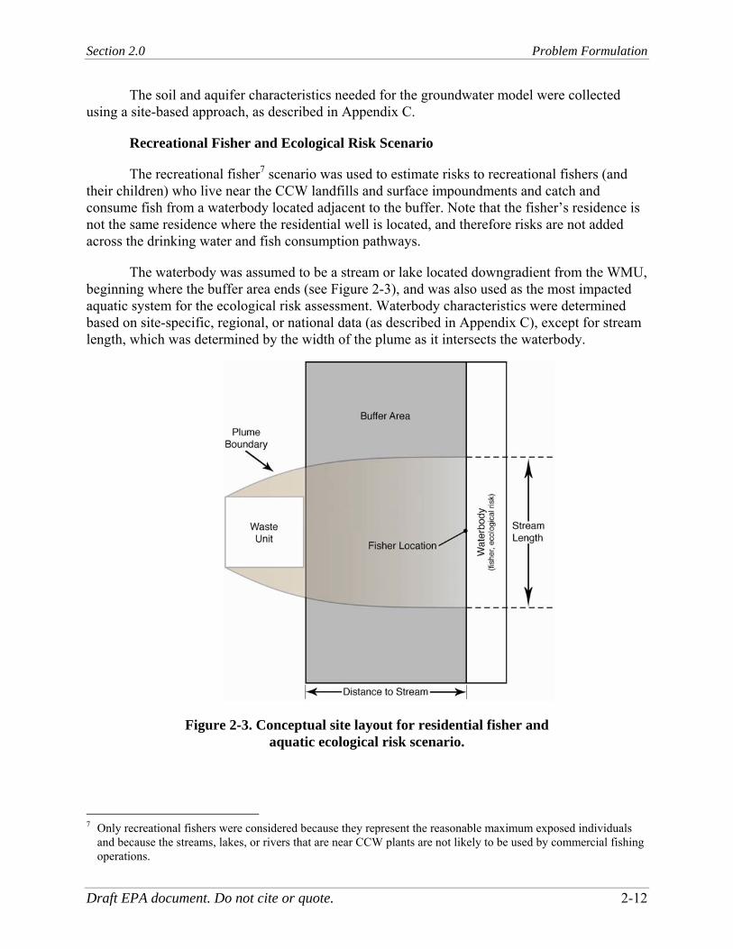
Section 2.0 Problem Formulation
Draft EPA document. Do not cite or quote. 2-12
The soil and aquifer characteristics needed for the groundwater model were collected using a site-based approach, as described in Appendix C.
Recreational Fisher and Ecological Risk Scenario
The recreational fisher7 scenario was used to estimate risks to recreational fishers (and their children) who live near the CCW landfills and surface impoundments and catch and consume fish from a waterbody located adjacent to the buffer. Note that the fisher’s residence is not the same residence where the residential well is located, and therefore risks are not added across the drinking water and fish consumption pathways.
The waterbody was assumed to be a stream or lake located downgradient from the WMU, beginning where the buffer area ends (see Figure 2-3), and was also used as the most impacted aquatic system for the ecological risk assessment. Waterbody characteristics were determined based on site-specific, regional, or national data (as described in Appendix C), except for stream length, which was determined by the width of the plume as it intersects the waterbody.
Figure 2-3. Conceptual site layout for residential fisher and aquatic ecological risk scenario.
7 Only recreational fishers were considered because they represent the reasonable maximum exposed individuals
and because the streams, lakes, or rivers that are near CCW plants are not likely to be used by commercial fishing operations.

Section 2.0 Problem Formulation
Draft EPA document. Do not cite or quote. 2-13
The downgradient distance to the surface water body was determined from a national distribution developed by measuring this distance (using scaled U.S. Geological Survey [USGS] maps and aerial photographs obtained from the Terraserver Web site [http://terraserver.usa.com/ geographic.aspx]) at 59 CCW landfill and surface impoundment sites randomly selected from a larger data set of 204 CCW WMUs, including those modeled in this risk assessment. Appendix C presents that distribution and further details on how the distribution was developed and the sample of 59 facilities used to develop the distribution.
2.3 Analysis Scope and Design
Although the screening analysis identified the potential for risk for a subset of the constituents reported in CCW, the conservative assumptions used precluded an accurate quantitative estimate of these risks. To gain a better understanding of the risks that may be posed by these constituents, EPA conducted a full-scale probabilistic (Monte Carlo) risk assessment to estimate the national distribution of the risks to human health and the environment posed by CCW disposal, and to provide the information needed to assess future management options for these wastes in the context of their risks to human health and the environment. The full-scale CCW Monte Carlo risk assessment was designed to characterize the national CCW risk profile in terms of WMU type, waste type, and constituent, and to use distributions in a probabilistic modeling framework to incorporate variability and uncertainty into the analysis.
The site-based approach used data about waste management practices and environmental conditions at 181 utility CCW disposal sites across the United States.8 These sites were assumed to represent the universe of CCW onsite waste disposal sites at the time of the EPRI survey (1995) and defined the national framework for the risk assessment. As described in Appendices B and C, site-specific data for the following model inputs were collected for these sites and used in the risk assessment:
WMU dimensions
WMU liner status (unlined, clay liner, composite liner)
Waste type (conventional CCW, CCW codisposed with coal refuse, and FBC wastes)
Geology (aquifer type)
Soil texture
Climate (precipitation, infiltration)
Surface water type and flow conditions.
One question related to this risk assessment is how CCW facilities may have changed in the decade since the 1995 EPRI survey. Although the DOE/EPA survey does not include all of
8 These 181 sites include177 sites from the EPRI survey and 4 additional CCW sites added by EPA to better
represent FBC waste disposal facilities; see Section 2.1.2.

Section 2.0 Problem Formulation
Draft EPA document. Do not cite or quote. 2-14
the data needed to conduct a risk assessment (WMU area and capacity data were not collected), liner conditions were addressed, and by comparing the DOE/EPA survey results to the EPRI data one can assess how liner conditions changed as CCW facilities were built or expanded over the past decade. The 56 WMUs surveyed in the U.S. DOE (2006) study were commissioned between 1994 and 2004. Although the actual number of WMUs that were established in that timeframe cannot be verified, based on proxy data (i.e., CCW available for disposal in those states with identified new WMUs and coal-fired power plant generating capacity), the sample coverage is estimated to be at least between 61 to 63 percent of the total population of the newly commissioned WMUs.9 With the exception of one landfill, the newly constructed facilities are all lined, with either clay, synthetic, or composite liners. The single unlined landfill identified in the recent DOE report receives bottom ash, which is characterized as an inert waste by the state, and therefore, a liner is not required. There is a marked trend away from unlined WMUs in favor of lined units, with a distinct preference for synthetic or composite liners. Comparison of the 26 coal combustion plants in both the EPRI survey and the DOE/EPA survey (U.S. DOE, 2006) shows that although most of those facilities (17 of 26) were using unlined WMUs in 1995, all 26 are now placing wastes in new or expanded landfills or surface impoundments that are lined with clay, synthetic, or composite liners. However, it is likely that the older unlined units were closed with wastes in place, and that these wastes therefore still pose a threat through groundwater pathways. In addition, the available data cannot be used to determine the number of unlined units that continue to operate in the United States.
Because site-specific data were not readily available for depth to groundwater or receptor location (i.e., distances to nearest drinking water well and surface waterbody), national distributions for those inputs taken from a national hydrogeologic database (Newell et al., 1989 and 1990) developed to support EPA’s national groundwater risk assessments were used in the Monte Carlo analysis to characterize the national variability of receptor distances (see Appendix C). This enabled EPA to assess the importance of those variables for the national risk distribution for individuals with reasonable maximum exposure to CCW.
The full-scale assessment was conducted using several modeling components: (1) EPA’s Composite Model for Leachate Migration with Transformation Products (EPACMTP; U.S. EPA, 1997a) groundwater model, (2) a simple steady-state surface water and aquatic food web model, and (3) a multipathway exposure and risk modeling system.
2.3.1 Data Collection
For the sites representing each WMU and waste type combination selected for analysis, the Monte Carlo analysis begins with input files that contain, for each Monte Carlo realization, the following site-based variables:
WMU area, depth, and capacity
WMU liner status
9 For additional details as to how these estimates were derived, the reader is referred to the DOE study, pages S-2
to S-3 of the Summary Section and Section 3.1.2.

Section 2.0 Problem Formulation
Draft EPA document. Do not cite or quote. 2-15
Soil texture (for vadose zone properties and infiltration rates)
Soil pH and organic carbon
Aquifer type
Groundwater temperature
Climate center (for infiltration rates)
USGS Hydrologic Region (for surface water quality data)
Surface water flows.
CCW constituent data in the CCW constituent database were used as a national empirical distribution of the concentrations of the constituents of concern in CCW landfill leachate and surface impoundment porewater. Like the WMU database, the CCW constituent data include WMU type and waste type, which enabled constituent concentrations to be assigned to the 181 CCW sites by waste type and WMU type. The CCW constituent database was also used to assign (by waste type) the high, medium, and low leachate pH and ionic strength conditions needed to select the appropriate subsurface sorption isotherms for each model run (see Appendix D).
National distributions were used to populate the following variables by model run:
Distance to nearest drinking water well
Distance to nearest surface waterbody
Aquifer depth, thickness, gradient, and hydraulic conductivity (based on site-specific hydrogeologic setting)
Soil hydrologic properties (based on site-specific soil type).
The data sources used to develop national distributions for these variables are described in Appendix C. Human exposure factors, such as exposure duration and drinking water and fish consumption rates, were also based on national distributions, which are provided in Appendix F.
2.3.2 Model Implementation
As a first step in the modeling process, the groundwater model (EPACMTP) reads the site-based data files to estimate the following for each model run:
Drinking water well peak concentration
Time to drinking water peak concentration
Peak surface water contaminant flux
Time to peak surface water contaminant flux.

Section 2.0 Problem Formulation
Draft EPA document. Do not cite or quote. 2-16
The groundwater model is run until contaminant concentrations at the receptor point return to zero after the concentration peak or for the maximum simulation time of 10,000 years, whichever comes first.
Groundwater model results are passed to the multimedia modeling system to estimate surface water and sediment concentrations and to calculate human and ecological exposure and risk. Additional inputs sent to the model at this stage include
Site-based surface waterbody type, dimensions, flows, pH, and total suspended solids (TSS) concentration
Chemical-specific fish bioconcentration factors (BCFs)
Human exposure factors (from national distributions)
Human and ecological health benchmarks.
For human health, the multimedia modeling system calculates risk from drinking water ingestion and fish consumption for each realization. For ecological risk, the model uses surface water and sediment concentrations along with ecological benchmarks to estimate the risks to ecological receptors.
2.3.3 Exposure Assessment
Table 2-5 lists the human and ecological receptors considered in the CCW risk assessment, along with the specific exposure pathways that apply to each receptor. All of the receptors that EPA considered were assumed to live offsite, at a location near the WMU.
Table 2-5. Receptors and Exposure Pathways Addressed in the Full-Scale CCW Assessment
Receptor
Ingestion of Drinking
Water Fish
Consumption
Direct Contact with Surface Water and Sediment
Ingestion of Aquatic
Organisms Human Receptors Adult resident U Child resident U Adult recreational fisher U Child recreational fisher U Ecological Receptors Aquatic and sediment organisms U Mammals and birds U
For human receptors, the exposure assessment estimates the dose to an individual receptor by combining modeled CCW constituent concentrations in drinking water or fish with intake rates for adult and child receptors. The full-scale CCW risk assessment considered

Section 2.0 Problem Formulation
Draft EPA document. Do not cite or quote. 2-17
exposures due to chemicals leaching from WMUs and contaminating groundwater. The groundwater exposures include drinking water ingestion and consumption of recreationally caught contaminated fish from surface waterbodies affected by contaminated groundwater. For the groundwater-to-drinking-water pathway, it was conservatively assumed that well water was the only source of drinking water (although some households may drink bottled or treated water or may drink water outside the home, e.g., at work or at school).
For ecological receptors, exposure assumptions are incorporated into the development of ecological benchmarks (see Appendix H), which are surface water and sediment concentrations corresponding to an HQ of 1.
The time period for the exposure assessment is defined by the peak concentration in the media of concern and the exposure duration. For human receptors, annual average media concentrations were averaged over the randomly selected exposure duration around the peak concentration for each run. To protect against chronic effects to ecological receptors, we consider the exposure duration over a significant portion of the receptor’s lifetime, and we believe that one year is the appropriate period of time for that. To be protective, we use the highest (peak) annual average concentration to estimate ecological exposure and risk.
2.3.4 Risk Estimation
Risk was estimated using several risk endpoints as particular measures of human health risk or ecological hazard. A risk endpoint is a specific type of risk estimate (e.g., an individual’s excess cancer risk) that is used as the metric for a given risk category. The CCW risk assessment evaluated cancer and noncancer endpoints for humans and noncancer endpoints for ecological receptors. For human risk, the availability of toxicological benchmarks for cancer and noncancer effects determined which endpoints were evaluated for each constituent.
EPA used two risk endpoints to characterize risk for the human receptors and a single risk endpoint, total HQ, to characterize risk for ecological receptors. These endpoints are discussed in Section 3.8; in addition, uncertainty related to these endpoints is discussed in Section 4.4.3.4.
From the distribution of risks for each risk endpoint generated by the Monte Carlo analysis, the 50th and 90th percentile risks were selected and compared to the risk criteria of 1 in 100,000 excess cancers and an HQ greater than 1 for noncarcinogens. An HQ greater than 1 for was also used for the ecological risk criterion in the full-scale risk assessment.


Section 3.0 Analysis
Draft EPA document. Do not cite or quote. 3-1
3.0 Analysis The full-scale analysis evaluates risks from CCWs disposed of in landfills and surface
impoundments located onsite at coal-fired utility power plants across the United States based primarily on data collected in 1995 by EPRI (1997).1 Chemical constituents found in CCW can be released from these WMUs into the surrounding environment by various mechanisms. Releases to the atmosphere and by erosion and overland transport did not pose risks above the screening criteria in the screening analysis; therefore, these were not assessed in the full-scale analysis. Instead, the full-scale analysis focused on groundwater pathways, which exceeded the risk criteria for some constituents in the screening analysis. Leachate forms in both landfills and surface impoundments, migrates from the WMU through soil to groundwater, and is transported in groundwater to drinking water wells (groundwater-to-drinking-water pathway) and into surface waterbodies near the WMU (groundwater-to-surface-water pathway). These are the groundwater pathways evaluated in the full-scale CCW risk assessment.
For the full-scale analysis, EPA used computer-based models and sets of equations to estimate the risk to human health and the environment from current CCW disposal practices.2 These models include
Source models that simulate the release of CCW constituents in leachate from landfills and surface impoundments3
Fate and transport models that estimate contaminant concentrations in groundwater and surface water
Exposure models that estimate daily contaminant doses for humans and ecological receptors exposed to CCW constituents in groundwater and surface water
Risk models that calculate risks to humans and ecological receptors.
This section describes the models and equations used to calculate exposure point concentrations and risk. Section 3.1 provides the overall structure for the analysis, including the spatial and temporal framework and the probabilistic (Monte Carlo) framework for the model runs. Sections 3.2 and 3.3 describe the landfill and surface impoundment source models used to predict environmental releases of constituents from CCW. Sections 3.4 and 3.5 describe the fate and transport modeling used to predict contaminant concentrations in groundwater and surface
1 The selection and characterization of these CCW WMUs are described in more detail in Appendix B. 2 As discussed in Section 2, the 1995 EPRI survey data is assumed to represent current CCW management
practices. However, new data from a more recent DOE/EPA survey suggest that liners may be more prevalent in new and expanded units built since 1994. Section 4 discusses implications of this uncertainty on the risk assessment results.
3 EPA used source-term models integrated into EPACMTP to estimate environmental releases of constituents in leachate from landfills and surface impoundments.

Section 3.0 Analysis
Draft EPA document. Do not cite or quote. 3-2
water. Section 3.6 describes the human exposure calculations. Section 3.7 describes the health benchmarks used to develop human and ecological risk estimates, and Section 3.8 describes how these risks were calculated for human and ecological receptors.
Supporting detail can be found in the following appendices:
Appendix A, Constituent Data, provides the CCW constituent concentrations used and describes how they were collected and processed
Appendix B, Waste Management Unit Data, describes the location and characteristics of each landfill and surface impoundment modeled and describes how the source model input parameter values were collected
Appendix C, Site Data, describes how environmental data around each CCW waste disposal site were collected to provide inputs for the groundwater and surface water modeling
Appendix D, MINTEQA2 Nonlinear Sorption Isotherms, describes the development and application of the CCW-specific MINTEQ metal sorption isotherms used to model fate and transport in soils and groundwater
Appendix E, Surface Water, Fish Concentration, and Contaminant Intake Equations, documents the algorithms used to calculate surface water concentrations, fish concentrations, and drinking water and fish intake rates
Appendix F, Human Exposure Factors, documents the human exposure parameters and equations
Appendix G, Human Health Benchmarks, describes how the human toxicity benchmarks were selected and developed
Appendix H, Ecological Benchmarks, describes how the ecological toxicity benchmarks were selected and developed.
3.1 General Modeling Approach
This section describes the framework, general assumptions, and constraints for the full-scale probabilistic analysis. Section 3.1.1 describes the temporal and spatial framework. Section 3.1.2 describes the probabilistic framework, and Section 3.1.3 describes how the assessment was implemented within the probabilistic framework.
3.1.1 Temporal and Spatial Framework
The spatial framework for the analysis was determined by the geographic distribution of CCW facilities modeled and by the site layout assumed as the conceptual site model for risk assessment. As described in Section 2.1.2, the geographic distribution of landfills and surface impoundments managing wastes onsite at coal-fired utility power plants was determined from

Section 3.0 Analysis
Draft EPA document. Do not cite or quote. 3-3
the 177 sites in the 1995 EPRI survey of the onsite management of CCW (EPRI, 1997). The assessment assumes that these 177 sites and their locations are representative of the approximately 300 coal-fired power plants identified by EIA data as having onsite waste management of conventional CCW and CCW codisposed with coal refuse throughout the United States. For FBC wastes, these 177 sites include only 3 FBC landfills. EPA was able to add 4 additional FBC landfill sites to better represent FBC waste management, for an overall total of 181 sites in this analysis.
The conceptual site layouts applied to each of the sites are described and pictured in Section 2.2.2. Two site layouts were used to define the relationship between a landfill or surface impoundment and (1) a drinking water well (for human risk via the groundwater-to-drinking-water pathway) and (2) a surface water body (for human and ecological risk via the groundwater-to-surface-water pathway). In each case, the receptor point (well or waterbody) was assumed to lie within the boundaries of the groundwater contaminant plume. The distance from the edge of the WMU to the well or waterbody was varied for each model run based on national distributions, with well distance taken from a national distribution for Subtitle D municipal landfills (U.S. EPA, 1988a) and distance to surface water taken from a set of measured distances for CCW landfills and surface impoundments developed for this assessment. Appendix C presents additional details on these distributions.
The temporal framework was mainly defined by the time of travel from the modeled WMU to the well or waterbody, which can be up to one mile away from the edge of the unit, and the exposure duration over which risks were calculated. The subsurface migration of some CCW constituents (e.g., lead) may be very slow; therefore, it may take a long time for the contaminant plume to reach the receptor well or nearest waterbody, and the maximum concentration may not occur until a very long time after the WMU ceases operations. This time delay may be on the order of thousands of years. To avoid excessive model run time while not missing significant risk at the receptor point, the groundwater model was run until the observed groundwater concentration of a contaminant at the receptor point dropped below a minimum concentration (10-16 mg/L) or until the model had been run for a time period of 10,000 years. The minimum concentration used for all fate and transport simulations (10-16 mg/L) is at least a million times below any risk- or health-based criteria.
For the groundwater-to-drinking-water pathway (human health risk), risks were calculated based on a maximum time-averaged concentration around the peak concentration at each receptor well. The exposure duration (which varies from 1 to 50 years)4 was applied around the peak drinking well concentration to obtain the maximum time-averaged concentration.
For the groundwater-to-surface-water pathway, the groundwater model produces surface water contaminant loads (based on groundwater concentration and flow) for a stream that penetrates the aquifer. Because the surface water model is a steady-state model, there is no temporal component to it and the receptor is exposed to the same concentration over the entire exposure duration. For human health risk, the loadings from groundwater to surface water were averaged over the exposure duration, bracketing the time of the peak groundwater concentration. 4 Distributions of exposure duration and other exposure variables were obtained from the Exposure Factors
Handbook (U.S. EPA, 1997c,d,e)

Section 3.0 Analysis
Draft EPA document. Do not cite or quote. 3-4
The exposure duration for sensitive ecological receptors is generally a year or less; therefore, for ecological risk, a single peak annual average surface water concentration was used.
For all scenarios, if the groundwater model predicted that the maximum groundwater concentration had not yet occurred after 10,000 years, the actual groundwater concentration at 10,000 years was used in the exposure calculations instead of a maximum time-weighted average concentration around the peak.
3.1.2 Probabilistic Approach
The full-scale analysis evaluates risk in a probabilistic manner and is based on a Monte Carlo simulation that produces a distribution of exposures and risks. The general Monte Carlo approach is shown in Figure 3-1. The foundation of the Monte Carlo simulation is the source data derived from the EPRI survey. These were combined with data from the national CCW constituent database to conduct a Monte Carlo simulation of 10,000 iterations per waste type/WMU type/constituent combination.
Waste Scenarios
Scenario(waste type x WMU x constituent)
Sample(constituent data)
Site(WMU data)
EPACMTP/SW model
Receptor
Pathway
WMU
ConstituentsIsotherms
Randomly located well
10,000
Randomly located waterbody
ChildGW->DW Risk
Adult
10,000Fish
ConsumptionRisk
Eco RiskFood chain
Direct contact
Exposure/Risk
iterations
iterations
Surface water concentrations
Receptor well concentrations
Child
Adult
Figure 3-1. Overview of the Monte Carlo approach.
The detailed looping structure for the Monte Carlo analysis is shown in Figure 3-2. For each waste type/WMU combination, two separate loops are run. The first loop (shown with dashed lines in Figure 3-2) prepares a set of input files containing 10,000 sets of WMU and site data (as described in Section 3.1.3). The second loop (shown with solid lines in Figure 3-2) uses those input files to run 10,000 iterations of the source, fate and transport, exposure, and risk models for each constituent.

Section 3.0 Analysis
Draft EPA document. Do not cite or quote. 3-5
Waste/WMU Scenario Loop
Next Waste/WMU Scenario
Human Receptor Loop
Next Constituent
Constituent Loop [Monte Carlo Loop]
Select 1 Waste type Conventional CCW, Codisposed CCW and coal refuse, FBC)Select 1 WMU type (landfill, surface impoundment)Data Preparation Loop:Select 1 Facility ID (EPRI survey)Pull data for Facility ID
Select 1 Aquifer Type (empirical distribution)Select 1 SoilType, with pH, OM (empirical distribution)Pull WMU data (area, depth, liner type)
Select distributed WMU data (missing depth, DBGS)Pull Climate CenterSelect 1 SampleID from Constituent database (pH table)
Pull leachate pHPull national data
Pull waste bulk density (=1.19), fraction CCW (=1), SI duration (=75 yr), SI sludge depth (0.2 m)Select 1 distance to surface water
Select next Facility ID
** Call EPACMTP to select soil data (by SoilType), aquifer data (by Aquifer Type), MINTEQA2 master variables, receptor well distance and calculate infiltration rate and vadose zone pH
Loop over 4 RecID: (1) adult resident, (2) child resident, (3) adult fisher, (4) fisher's child
Select pathways, exposure factors based on RecID:Pull benchmarks
** Call Exposure Module to calculate ADD, LADD for each pathway** Call Risk Module and calculate cancer risk, HQ for each pathway
RunID Loop (10,000 iterations)Select 1 Facility ID (with data from data preparation loop)
Pull surface water type, flow dataSelect 1 SampleID from Constituent Database
Pull 1 leachate concentrationPull (or calculate) 1 corresponding total waste concentration (landfills only)
Pull nationally distributed data from data preparation loopSelect 1 SW TSS
** Call EPACMTP to calculate drinking water concentration (random and 150m well) and surface water flux [output based on exposure durations]
** Call SW Module to calculate surface water and sediment concentrations** Call Food Web Module to calculate fish concentration
Next RunID
Next Receptor
Select 1 Constituent (11 priority metals and nitrate/nitrite)
Ecological RiskPull ecological benchmarks (CSCLs)** Calculate SW and sediment HQs
Monte Carlo Loop
Data preparation loop
** indicates model runsADD = average daily doseDBGS = depth below ground surfaceHQ = hazard quotientLADD = lfetime average daily dose
Figure 3-2. Monte Carlo looping structure.

Section 3.0 Analysis
Draft EPA document. Do not cite or quote. 3-6
3.1.3 Implementation of Probabilistic Approach
Table 3-1 lists the five waste disposal scenarios addressed in the full-scale analysis. FBC waste landfills were modeled and treated as a separate scenario in the analysis because of the limited number (7) of FBC landfill sites. Each waste disposal scenario modeled in the full-scale assessment included unlined, clay-lined, and composite-lined WMUs. Additional detail on these scenarios can be found in Section 2-1 and Appendix A.
Table 3-1. CCW Waste Management Scenarios Modeled in Full-Scale Assessment
WMU Type Waste Type Conventional CCW and CCW Codisposed with Coal Refuse (main analysis)
Landfill Conventional CCW (fly ash, bottom ash, boiler slag, FGD sludge)
Landfill Codisposed CCW and coal refuse Surface impoundment Conventional CCW Surface impoundment Codisposed CCW and coal refuse FBC Waste (separate analysis) Landfill FBC waste (fly ash, bottom ash, bed ash)
To capture the national variation in waste management practices for the Monte Carlo analysis, an input database was created with approximately 10,000 iterations for each of the waste type/WMU combinations. This input database provided the source data for 10,000 iterations of the source modeling and the fate and transport modeling. Figure 3-3 provides an overview of the process used to compile these data, which were organized into source data files. As shown in Figure 3-3, seven tasks, some parallel and some sequential, were required to construct these data files, one file for each waste management scenario.
Constructing the source data files for use in the probabilistic analysis involved first developing a 10,000-record data file for each waste type-WMU scenario. This was accomplished by selecting the landfills and surface impoundments from the EPRI survey data that manage each type of waste. Within a scenario, a list of the EPRI plants with that WMU type and waste type was repeated to produce around 10,000 records. For each record, site-based, regional, and national inputs were randomly selected from distributions developed to characterize the regional or national variability in these inputs. Each record in the source data files was identified by a model run identification number (RunID).
The EPRI survey provided most of the WMU data needed, including area, capacity, liner type, and waste type. Additional data were collected to characterize the height and depth below ground surface of typical CCW landfills and surface impoundments (see Appendix B).
The environmental setting in which waste disposal occurs was characterized based on the location of the 181 power plants used in the full-scale analysis. These locations were used to characterize climate, soils, aquifers, and surface water bodies at each site as follows (see Appendix C for details):

Section 3.0 Analysis
Draft EPA document. Do not cite or quote. 3-7
Figure 3-3. Process used to construct the Monte Carlo input database.
Climatic data, including annual precipitation, temperature, and windspeed, were collected by assigning each site to a nearby meteorologic station.
Soil and aquifer type were collected within a 5-km radius of each site to account for locational uncertainty for the WMUs.
Surface water type and flows were collected using a geographic information system (GIS) to identify the nearest stream and by matching plants to the Permit Compliance

Section 3.0 Analysis
Draft EPA document. Do not cite or quote. 3-8
System (PCS) database to get the stream segment for each plant’s NPDES discharge point.
These site-based data were supplemented with regional data on surface water quality and with national distributions of receptor distances (i.e., distance to drinking water well and distance to nearest surface waterbody). Appendix C describes the site-based approach and data sources used for these site-specific, regional, and national-scale data collection efforts.
The five 10,000-record scenario-specific source data files were then combined with the CCW constituent data for each constituent in the appropriate waste type to develop the final source data files for each scenario. With 12 constituents modeled for most scenarios, this resulted in over 600,000 records in the final input data set.
3.2 Landfill Model
Releases from landfills were modeled using a landfill source-term model contained in EPACMTP. EPA has used EPACMTP and its predecessor models for almost 20 years to conduct groundwater risk assessments in support of regulations for land disposal of hazardous and nonhazardous wastes. In that context, EPACMTP has undergone numerous peer reviews, including multiple reviews by EPA’s Science Advisory Board (SAB). Each of these reviews has supported and approved the use of this model for developing national regulations and guidance, including verification that the model and model code are scientifically sound and properly executed. Some of the more important reviews include
A 1989 review by SAB of the component saturated zone (groundwater) model used in EPACMTP
A 1993 review by EPA’s Office of Research and Development (ORD) of EPACMTP for potential Hazardous Waste Identification Rule applications, which resulted in a number of improvements in the computational modules of EPACMTP
A 1994 consultation with SAB on the use of EPACMTP for determination of dilution-attenuation factors for EPA’s Soil Screening Guidance
A 1994 review by expert modelers Dr. Fred Molz (Auburn University) and Mr. Chris Neville (SS Papadopoulos & Associates), who verified that the mathematical formulation of the model and the code verification testing are scientifically sound
The peer-reviewed publication of EPACMTP in the Journal of Contaminant Hydrology (Kool et al., 1994)
An in-depth review by SAB related to the use of EPACMTP in the proposed/draft 1995 Hazardous Waste Identification Rule (U.S. EPA, 1995)
A 1999 peer review by leading modelers of the implementation of EPACMTP in EPA’s multimedia, multiple exposure pathway, multiple receptor risk assessment (3MRA) model (U.S. EPA, 1999c)

Section 3.0 Analysis
Draft EPA document. Do not cite or quote. 3-9
A 2003 SAB review of the 3MRA implementation of EPACMTP (SAB, 2004).
An overview and statement of assumptions for the landfill model is presented here, followed by a listing of inputs to the landfill source-term model and a brief discussion of the output generated by the model.
3.2.1 Conceptual Model
The landfill model treats a landfill as a permanent WMU with a rectangular footprint and a uniform depth (see Figure 3-4). If only the area is known (which is the case for the CCW landfills), the landfill source-term model assumes a square footprint. The model assumes that the landfill is filled with waste during the unit’s operational life and that upon closure of the landfill, the waste is left in place and a final soil cover is installed.
Figure 3-4. Conceptualization of a landfill in the landfill source-term model.
Three liner scenarios were modeled: a no-liner (unlined) scenario, a compacted clay liner, and a composite liner that combines a high-density polyethylene (HDPE) membrane with either geosynthetic or natural clays.
In the unlined scenario, waste is placed directly on local soils, either on grade or excavated to some design depth and without a leachate collection system. After the landfill has been filled to capacity, a 2-foot native soil cover (the minimum required by Subtitle D regulations) is installed and assumed to support vegetation.
In the clay liner scenario, waste is placed directly on a 3-foot compacted clay liner, which is installed on the local soils, either on grade or excavated to some design depth and without a

Section 3.0 Analysis
Draft EPA document. Do not cite or quote. 3-10
leachate collection system. After the landfill has been filled to capacity, a 3-foot clay cover is installed and covered with 1 foot of loam to support vegetation and drainage. The hydraulic conductivity of both the liner and cover clays is assumed to be 1x10⁻⁷ cm/sec, the typical design specification for compacted clay liners (U.S. EPA, 1988c).
In the composite liner scenario, wastes are placed on a liner system that consists of a 60 mil HDPE membrane with either an underlying geosynthetic clay liner or a 3-foot compacted clay liner. A leachate collection system is also assumed to exist between the waste and the liner system. After the landfill has been filled to capacity, a 3-foot clay cover is assumed to be installed and covered with 1 foot of loam to support vegetation and drainage (U.S. EPA, 2002b).
As described in Section 3.2.3 (and Appendix B), one of these three liner types was assigned to each CCW landfill or surface impoundment modeled based on the liner type data from the 1995 EPRI Survey (EPRI, 1997).
3.2.2 Modeling Approach and Assumptions
The starting point for the landfill source-term model simulation is the time when the landfill is closed (i.e., when the unit is filled with CCW).5 As described in detail below, the full-scale analysis modeled contaminants leaching from CCW into precipitation infiltrating the landfill, which exits the landfills as leachate. Contaminant loss in leachate was taken into account at closure by subtracting the cumulative amount of contaminant mass loss that occurred during the unit’s active life from the amount of contaminant mass present at the time of landfill closure. Loss calculations in the landfill source-term model continue after closure until the contaminant is depleted from the waste mass in the landfill. This is a conservative assumption, as some metal will not leach from the waste mass.
Infiltration and Leaching
The average rate at which water percolates through the landfill over time (the long-term infiltration rate) drives the leaching process in the landfill, which results from partitioning of the constituent from the waste into the infiltrating water. The methodology, assumptions, and data used to determine infiltration rates for each CCW liner scenario are consistent with the approach used in EPA’s Industrial D guidance, as described in Section 4.3 and Appendix A of the EPACMTP Parameter/Data Background Document (U.S. EPA, 2003a) and Section 4.2.2 of the Industrial Waste Evaluation Model (IWEM) Technical Background Document (U.S. EPA, 2002b). EPA developed the IWEM model as part of a guide for managing nonhazardous industrial wastes in landfills and surface impoundments (http://www.epa.gov/industrialwaste). To help ensure that it was technically sound, the model (including the liner scenarios and algorithms used in the CCW risk assessment) was developed with a large stakeholder working group, including representatives from industry. The model was also subjected to a peer review in 1999 (64 FR 54889–54890, October 8, 1999, Peer Reviews Associated With the Guide for
5 The simple landfill model used in this assessment cannot model a landfill as it is being filled prior to closure.
Although leaching does occur during a landfill’s operating life, risks from these releases are insignificant when compared to postclosure releases, given the long time it takes metal-bearing wastes to leach and reach peak concentrations in groundwater wells surrounding the landfill. EPA does not believe that the additional risks from the preclosure period justify the additional complexity, data, and effort required to model an operating landfill.

Section 3.0 Analysis
Draft EPA document. Do not cite or quote. 3-11
Industrial Waste Management), and the model was updated and improved in response to those comments before its final release in 2003. That update included the addition of a more robust liner leakage database to support the existing algorithms for calculating infiltration rates through composite liner systems.
No-Liner (Unlined) Scenario. For the no-liner scenario, infiltration rates were selected from a database in EPACMTP that contains 306 infiltration rates already calculated using EPA’s Hydrologic Evaluation of Landfill Performance (HELP) water balance model (Schroeder, et al., 1994a, 1994b). HELP is a product of an interagency agreement between EPA and the U.S. Army Corps of Engineers Waterways Experiment Station, and was subjected to the Agency’s peer and administrative review. All of the infiltration rates were calculated based on the single typical landfill design described in Section 3.2.1, with the only variables that change between HELP simulations being the meteorological data associated with 102 nationwide climate centers and the type of cover soil applied at closure. Three cover soil categories representing coarse-grained soils, medium-grained soils, and fine-grained soils were used. The selection of an infiltration rate from the database depends on the type of cover soil selected for the landfill and the assignment of the landfill to a HELP climate center. The unlined HELP-derived infiltration rates are presented in U.S. EPA (2003a) by climate center. The assignment of HELP climate centers and soil categories to each CCW site modeled is described in Appendix C.
Clay Liner Scenario. The clay liner scenario is very similar to the unlined scenario in that previously calculated HELP infiltration rates for a single clay-lined, clay-capped landfill design were used. The scenario is based on a typical engineered compacted clay liner that is 3 feet thick with a design hydraulic conductivity of 1x10⁻⁷ cm/sec. The one difference from the unlined case is that the clay liner and cover control the rate of water percolation through the landfill and thus infiltration rate does not vary with cover soil (i.e., there is one clay liner infiltration rate per climate center). The clay liner HELP-derived infiltration rates are provided in U.S. EPA (2003a).
Composite Liner Scenario. Composite liner infiltration rates are compiled from monthly average leak detection system (LDS) flow rates for industrial landfill cells reported by TetraTech (2001). The liner configurations are consistent with the composite liner design assumptions presented in Section 3.2.1 and are the same as those assumed for defaults in EPA’s Industrial D landfill guidance (U.S. EPA, 2002b). The LDS flow rates were taken from 27 municipal landfill cells and used in the IWEM model (U.S. EPA, 2002b). As shown in Table 3-2, these LDS flow rates include 22 operating landfill cells and 5 closed landfill cells located in eastern United States: 23 in the northeastern region, 1 in the mid-Atlantic region, and 3 in the southeastern region. Each of the landfill cells is underlain by a geomembrane/geosynthetic clay liner which consists of a high-density polyethylene geomembrane of thickness between 1 and 1.5 mm, overlying a 6-mm composite geosynthetic clay layer consisting of two geotextile outer layers with a uniform core of bentonite clay to form a hydraulic barrier. Each liner system is underlain by an LDS.
As described in U.S. EPA (2002b), only a subset of the TetraTech (2001) flow rates were used to develop the composite liner infiltration rates. LDS flow rates for geomembrane/ compacted clay composite-lined landfill cells were not used in the distribution because compacted clay liners (including composite geomembrane/compacted clay liners) can release

Section 3.0 Analysis
Draft EPA document. Do not cite or quote. 3-12
water during consolidation and contribute an unknown amount of water to LDS flow, which makes it difficult to determine how much of the LDS flow is due to liner leakage versus clay consolidation. Also, LDS flow rates from three geomembrane/geosynthetic clay lined-cells were not used. For one cell, postclosure flow rates were very high, and were more than twice as high as those recorded during the cell’s operating period. Data were not used for two other cells because of inconsistencies with the data for the 27 landfill cells used to develop composite liner infiltration rates (U.S. EPA, 2002b). The composite liner infiltration rates were specified as an empirically distributed input to the landfill model (see U.S. EPA ,2003a).
Table 3-2. Leak Detection System Flow Rate Data Used to Develop Landfill Composite Liner Infiltration Rates
Cell ID Status Flow rate (m/y) Location G228 Operating 2.1E-04 Mid-Atlantic G232 Operating 4.0E-04 Northeast G232 Closed 7.3E-05 Northeast G233 Operating 0 Northeast G233 Closed 0 Northeast G234 Operating 7.3E-05 Northeast G234 Closed 0 Northeast G235 Operating 1.5E-04 Northeast G235 Closed 3.7E-05 Northeast G236 Operating 3.7E-05 Northeast G236 Closed 0 Northeast G237 Operating 7.3E-05 Northeast G238 Operating 0 Northeast G239 Operating 7.3E-05 Northeast G240 Operating 0 Northeast G241 Operating 0 Northeast G242 Operating 0 Northeast G243 Operating 0 Northeast G244 Operating 0 Northeast G245 Operating 0 Northeast G246 Operating 0 Northeast G247 Operating 0 Northeast G248 Operating 0 Northeast G249 Operating 7.3E-05 Northeast G250 Operating 2.2E-04 Southeast G251 Operating 0 Southeast G252 Operating 0 Southeast Source: U.S. EPA (2002a); original data from TetraTech (2001).
Source Depletion and Mass Balance
For this assessment, the landfill source-term model represents releases from landfills as a finite source where the mass of a constituent in a landfill is finite and depleted over time by

Section 3.0 Analysis
Draft EPA document. Do not cite or quote. 3-13
leaching. The landfill source-term model is set as a pulse source, where the leachate concentration is constant over a prescribed period of time and then goes to zero when the constituent is depleted from the landfill. A pulse source is appropriate for metals and other constituents whose sorption behavior is nonlinear. Because all but one (nitrate/nitrite) of the constituents addressed in the full-scale analysis are metals, releases from landfills were modeled as pulse sources.
For a pulse source, basic mass balance considerations require leaching from the landfill to stop when all of the constituent mass has leached from the landfill. For the constant concentration pulse source condition, the pulse duration is given by
SINFILCZERO
CTDENSFRACTDEPTHCWASTETSOURC×
×××= (3-1)
where
TSOURC = Pulse duration (yr) CWASTE = Constituent concentration in the waste (mg/kg) DEPTH = Depth of landfill (m) FRACT = Volume fraction of the landfill occupied by the waste (unitless) CTDENS = Waste density (g/cm3) CZERO = Initial waste leachate concentration (mg/L) SINFIL = Annual areal infiltration rate (m/yr).
The landfill source-term model uses the above relationship to determine the leaching duration. More details regarding the waste concentration and WMU parameters in Equation 3-1 are provided below and in Appendices A and B.
3.2.3 Landfill Model Input Parameters
Input parameters required by the landfill source-term model are discussed below. Additional details on how data for these inputs were collected for the CCW risk assessment are provided in Appendix A for leachate and waste concentrations and Appendix B for landfill dimensions and characteristics.
Landfill Area. The model uses landfill area to determine the area over which infiltration rate occurs and, along with landfill depth and waste concentration, to calculate the total contaminant mass in the landfill. CCW landfill area data were obtained from the EPRI comanagment survey (EPRI, 1997). The landfill was assumed to be square.
Landfill Depth. Landfill depth is one of several parameters used by the landfill source-term model to calculate the contaminant mass in the landfill. For CCW landfills, average waste depth was estimated by dividing landfill capacity by landfill area. CCW landfill capacity data were taken from the EPRI comanagement survey (EPRI, 1997).

Section 3.0 Analysis
Draft EPA document. Do not cite or quote. 3-14
Depth Below Grade. The depth of the bottom of the landfill below the surrounding ground surface is used, along with depth to groundwater, to determine the thickness of the unsaturated zone. For CCW landfills, depth below grade was determined from a national distribution based on available measurements from a number of CCW landfills (see Appendix B).
Waste Fraction. The landfills were assumed to be CCW monofills, which corresponds to a waste fraction of 1.0.
Waste Density. The average waste bulk density, as disposed, is used to convert waste volume to waste mass. The waste bulk density for all CCW waste types was assumed to be 1.19 g/cm3 (U.S. EPA, 1998b).
Leachate Concentration. The concentration of waste constituents in leachate was assumed to be constant until all of the contaminant mass initially present in the landfill has leached out, after which the leachate concentration was assumed to be zero. The constant value used for leachate concentration is from EPA’s CCW Constituent Database, described in Appendix A.
Waste Concentration. In the finite-source scenario modeled, the total waste concentration is used, along with the waste bulk density and landfill area and depth, to determine the total amount of a constituent available for leaching. Measured total CCW concentrations were paired with leachate concentrations, as described in Appendix A and provided in Attachment A-2.
Liner Type. The type of liner is used to determine the infiltration/leaching scenario used to calculate leachate flux from the landfill. Table 3-3 shows the crosswalk used to assign one of the three liner scenarios to each facility based on the liner data in the 1995 EPRI survey (EPRI, 1997). Attachment B-2 to Appendix B provides these assignments, along with the original EPRI liner type, for each CCW landfill facility modeled. One significant uncertainty in these liner assumptions is how representative the EPRI survey data are of current conditions at coal combustion facilities.
Table 3-3. Crosswalk Between EPRI and CCW Source Model Liner Types
EPRI Liner Type Model Liner
Code Description Compacted ash 0 no liner Compacted clay 1 clay Composite clay/membrane 2 composite Double 2 composite Geosynthetic membrane 2 composite None/natural soils 0 no liner
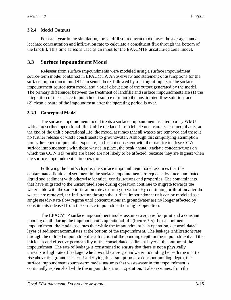
Section 3.0 Analysis
Draft EPA document. Do not cite or quote. 3-15
3.2.4 Model Outputs
For each year in the simulation, the landfill source-term model uses the average annual leachate concentration and infiltration rate to calculate a constituent flux through the bottom of the landfill. This time series is used as an input for the EPACMTP unsaturated zone model.
3.3 Surface Impoundment Model
Releases from surface impoundments were modeled using a surface impoundment source-term model contained in EPACMTP. An overview and statement of assumptions for the surface impoundment model is presented here, followed by a listing of inputs to the surface impoundment source-term model and a brief discussion of the output generated by the model. The primary differences between the treatment of landfills and surface impoundments are (1) the integration of the surface impoundment source term into the unsaturated flow solution, and (2) clean closure of the impoundment after the operating period is over.
3.3.1 Conceptual Model
The surface impoundment model treats a surface impoundment as a temporary WMU with a prescribed operational life. Unlike the landfill model, clean closure is assumed; that is, at the end of the unit’s operational life, the model assumes that all wastes are removed and there is no further release of waste constituents to groundwater. Although this simplifying assumption limits the length of potential exposure, and is not consistent with the practice to close CCW surface impoundments with these wastes in place, the peak annual leachate concentrations on which the CCW risk results are based are not likely to be affected, because they are highest when the surface impoundment is in operation.
Following the unit’s closure, the surface impoundment model assumes that the contaminated liquid and sediment in the surface impoundment are replaced by uncontaminated liquid and sediment with otherwise identical configurations and properties. The contaminants that have migrated to the unsaturated zone during operation continue to migrate towards the water table with the same infiltration rate as during operation. By continuing infiltration after the wastes are removed, the infiltration through the surface impoundment unit can be modeled as a single steady-state flow regime until concentrations in groundwater are no longer affected by constituents released from the surface impoundment during its operation.
The EPACMTP surface impoundment model assumes a square footprint and a constant ponding depth during the impoundment’s operational life (Figure 3-5). For an unlined impoundment, the model assumes that while the impoundment is in operation, a consolidated layer of sediment accumulates at the bottom of the impoundment. The leakage (infiltration) rate through the unlined impoundment is a function of the ponding depth in the impoundment and the thickness and effective permeability of the consolidated sediment layer at the bottom of the impoundment. The rate of leakage is constrained to ensure that there is not a physically unrealistic high rate of leakage, which would cause groundwater mounding beneath the unit to rise above the ground surface. Underlying the assumption of a constant ponding depth, the surface impoundment source-term model assumes that wastewater in the impoundment is continually replenished while the impoundment is in operation. It also assumes, from the

Section 3.0 Analysis
Draft EPA document. Do not cite or quote. 3-16
beginning of the unit’s operation, that the sediment is always in equilibrium with the wastewater (i.e., the presence of sediment does not alter the concentration of leachate). Accordingly, the surface impoundment source-term model also assumes that the leachate concentration is constant during the impoundment operational life. Typically, the leachate concentration is equal to the concentration in the wastewater entering the impoundment.
Figure 3-5. Schematic cross-section view of surface impoundment.
Three liner scenarios were modeled: a no-liner (unlined) scenario, a compacted clay liner, and a composite liner.
In the unlined scenario, wastewater is placed directly on local soils and the depth of water is constant over the entire life of the impoundment, pre- and post-closure. As described above, sediments accumulate and consolidate at the bottom of the impoundment and migrate into the underlying native soils, where they clog pore spaces and provide some barrier to flow. The surface impoundment model assumes that the thickness of the consolidated sediments is equal to one-half of the total sediment thickness, which is an input to the model. The sediment thickness was assumed to be 0.2 m for all simulations. The model also assumes that the thickness of the clogged region of native soils is always 0.5 m and has a hydraulic conductivity 10 percent of that of the native soil underlying the impoundment.
In the clay liner scenario, wastewater is placed on a compacted clay liner, which is installed on the local soils. The assumptions for an unlined impoundment also apply to the compacted clay liner scenario, except that a compacted clay liner filters out the sediments that clog the native soils in the unlined case, so the effect of clogging the native materials is not included in the calculation of the infiltration rate. The thickness of the compacted clay liner was assumed to be 3 feet and the hydraulic conductivity was assumed to be 1x10⁻⁷ cm/sec (U.S. EPA, 1988c).
In the composite liner scenario, wastewater is placed on a synthetic membrane with an underlying geosynthetic or natural compacted clay liner with a hydraulic conductivity of 1x10⁻⁷ cm/sec. The membrane liner was assumed to have a number of pinhole leaks of uniform size

Section 3.0 Analysis
Draft EPA document. Do not cite or quote. 3-17
(6 mm2). The distribution of leak densities (expressed as number of leaks per hectare) was compiled from 26 leak density values reported in TetraTech (2001), the best available data on liner leaks. These leak densities are based on liners installed with formal construction quality assurance (CQA) programs. The 26 sites with leak density data are mostly located outside the United States: 3 in Canada, 7 in France, 14 in the United Kingdom, and 2 in unknown locations; we assume that these are representative of U.S. conditions. The WMUs at these sites (8 landfills, 4 surface impoundments, and 14 of unknown type) are underlain by a layer of geomembrane with a thickness varying from 1.14 mm to 3 mm. The majority of the geomembranes (23 of 26) are made from HDPE, and the remaining 3 are made from prefabricated bituminous geomembrane or polypropylene. One of the sites has a layer of compacted clay liner beneath the geomembrane; however, for 25 of the 26 sites, material types below the geomembrane layer are not reported. The empirical distribution used in the analysis can be found in IWEM (U.S. EPA, 2002b), along with a table showing details about the 26 liners used to develop the distribution.
3.3.2 Modeling Approach and Assumptions
Figure 3-5 illustrates a compartmentalized surface impoundment with stratified sediment. Shown in the figure are the liquid compartment, the sediment compartment (with loose and consolidated sediments), and the unsaturated zone (with clogged and unaffected native materials). The model assumes that all sediment layer thicknesses remain unchanged throughout the life of the unit.
The EPACMTP surface impoundment model uses the unsaturated zone flow model to calculate the infiltration rate out of the bottom of the impoundment. This model is designed to simulate steady-state downward flow through an unsaturated (vadose) zone consisting of one or more soil layers. Steady-state means that the rate of flow does not change with time. In the case of flow out of an unlined surface impoundment, the model simulates flow through a system consisting of three layers: a consolidated sediment layer, a clogged soil layer, and a native soil layer.
The native unsaturated soil extends downward to the water table. The steady-state infiltration rate out of the surface impoundment is driven by the head gradient between the water ponded in the impoundment and the head at the water table. The pressure head at the top of the consolidated sediment layer is equal to the water depth in the impoundment plus the thickness of the unconsolidated sediment.
The EPACMTP Technical Background Document (U.S. EPA, 2003c) describes the algorithms used in this model to calculate the infiltration rate from surface impoundment units, and discusses in detail the maximum allowable infiltration rate based on the groundwater mounding condition. This information is summarized here.
The EPACMTP surface impoundment source-term model calculates infiltration through the accumulated sediment at the bottom of an impoundment, accounting for clogging of the native soil materials underlying the impoundment, liner conditions, and mounding due to infiltration. The modeled infiltration is governed by the depth of liquid in the impoundment and the following limiting factors:

Section 3.0 Analysis
Draft EPA document. Do not cite or quote. 3-18
Effective hydraulic conductivity and thickness of the consolidated sediment layer. As sediment accumulates at the base of the impoundment, the weight of the liquid and upper sediments tends to compress (or consolidate) the lower sediments. The consolidation process reduces the hydraulic conductivity of the sediment layer, and the layer of consolidated sediment will act as a restricting layer for flow out of the impoundment. By contrast, the layer of loose, unconsolidated sediment that overlies the consolidated sediment layer is assumed not to restrict the flow rate out of the unit, so it is not explicitly considered in the surface impoundment flow model.
Effective hydraulic conductivity of the clogged native material. As liquids infiltrate soil underlying the impoundment, suspended particulate matter accumulates in the soil pore spaces, reducing hydraulic conductivity and lowering infiltration rates.
Effective hydraulic conductivity and thickness of a clay liner. When the surface impoundment is underlain by a compacted clay liner, the rate of infiltration is also determined by simulating flow through a three-layer system, substituting the characteristics of the clay liner for those of the clogged soil layer.
Leak rate of a composite liner. For cases where the surface impoundment is underlain by a composite liner (a geomembrane underlain by a low permeability liner such as a compacted clay liner or a geosynthetic clay liner), the surface impoundment source-term model uses a modified equation of Bonaparte et al. (1989) to calculate the infiltration rate. The equation uses, among other inputs, the head generated by the water and unconsolidated sediments in the unit, a leak density selected from an empirical distribution derived from a TetraTech (2001) study of liner leakage, a uniform leak size of 6 mm2, and an assumed hydraulic conductivity of 1x10⁻⁷ cm/sec for the 3 feet of underlying compacted clay material.
Limitations on maximum infiltration rate from mounding. If the calculated infiltration rate exceeds the rate at which the saturated zone can transport the groundwater, the groundwater level will rise into the unsaturated zone. The model accounts for groundwater mounding when calculating the infiltration rate from the surface impoundment unit and, if necessary, constrains the value to ensure that the groundwater mound does not rise to the bottom of the surface impoundment unit.
3.3.3 Surface Impoundment Model Input Parameters
Input parameters required by the surface impoundment source-term model are discussed below. Additional details on how data for these inputs were collected for the CCW risk assessment are provided in Appendix A for waste concentrations and Appendix B for surface impoundment dimensions and characteristics.
Surface Impoundment Area. The model uses surface impoundment area to determine the area over which infiltration occurs. CCW surface impoundment area data were obtained from the EPRI comanagement survey (EPRI, 1997). The impoundment was assumed to be square.

Section 3.0 Analysis
Draft EPA document. Do not cite or quote. 3-19
Areal Infiltration Rate. The surface impoundment leachate infiltration rate (or flux) is computed internally by the surface impoundment source-term model, as described in Section 3.3.2.
Depth Below Grade. The depth of the bottom of the impoundment below the surrounding ground surface is used, along with depth to groundwater, to determine the thickness of the unsaturated zone beneath the impoundment. For CCW impoundments, depth below grade was sampled from an empirical distribution based on available measurements from a number of CCW surface impoundments (see Appendix B).
Operating Depth. The operating (or ponding) depth is the long-term average depth of wastewater and sediment in the impoundment, measured from the base of the impoundment. For CCW surface impoundments, depth was estimated by dividing impoundment capacity by impoundment area. CCW impoundment capacity data were taken from the EPRI comanagement survey (EPRI, 1997).
Total Thickness of Sediment. By default, EPACMTP models unlined surface impoundments with a layer of “sludge” or sediment above the base of the unit. The sediment layer is divided into two sublayers: an upper, loose sediment sublayer and a lower, consolidated sediment sublayer. The consolidated sediment has a relatively low hydraulic conductivity and acts to impede flow. The calculated infiltration rate is inversely related to the thickness of the consolidated sediment sublayer. A thinner consolidated sediment layer will result in a higher infiltration rate and a greater rate of constituent loss from the impoundment. The surface impoundment source-term model uses the total sediment thickness as an input parameter and assumes that it consists of equal thicknesses of loose and consolidated material. Because data were not available on CCW sediment layer thicknesses, the CCW risk assessment used the Tier 1 IWEM model assumption: a total (unconsolidated plus consolidated) sediment layer thickness of 0.2 meters (U.S. EPA, 2002b). It is not known how representative this assumption is with respect to unlined CCW surface impoundments, but it is reasonable to assume that a sediment layer would accumulate and restrict flow from the bottom of a CCW impoundment.
Distance to the Nearest Surface Water Body. The distance to the nearest waterbody is used to determine the location of a fully penetrating surface waterbody at which groundwater mass and water fluxes will be calculated and reported. The distance to the nearest surface waterbody is also used as a surrogate for the distance to the nearest point at which the water table elevation is kept at a fixed value. That distance is used to calculate the estimated height of groundwater mounding underneath the impoundment to ensure that excessively high infiltration rates, which may be calculated for deep, unlined impoundments, do not occur. If necessary, the model reduces the infiltration rate to ensure the predicted water table does not rise above the ground surface. For the CCW sites, distance to surface water was sampled from an empirical distribution developed from aerial photo measurements at 59 coal-fired power plants with onsite landfills or surface impoundments (Appendix C).

Section 3.0 Analysis
Draft EPA document. Do not cite or quote. 3-20
Leachate Concentration. The annual average leachate concentration is modeled as a constant concentration pulse with a defined duration. For a particular model run, the leachate concentration was assumed to be constant during the operation of the unit; there is no reduction in leachate concentration until the impoundment ceases operation. Leachate concentrations for CCW impoundments were obtained by waste type from surface impoundment porewater data from EPA’s CCW Constituent Database, as described in Appendix A.
Source Leaching Duration. For surface impoundments, the addition and removal of waste during the operational life period are more or less balanced, without significant net accumulation of waste. In the finite-source implementation used for CCW surface impoundments, the duration of the leaching period is assumed to be the same as the operational life of the surface impoundment. Based on industry data (see Appendix B) for CCW surface impoundments, we used a high-end (90th percentile) fixed surface impoundment operating life of 75 years. A high-end value was appropriate because CCW surface impoundments are typically closed with waste in place, while the surface impoundment source-term model assumes clean closure (waste removed). In addition, operating life is not a particularly sensitive parameter in this analysis: the difference between the 50th percentile value (40 years) and the 90th percentile value used (75 years) is less than a factor of two.
Liner Type, Thickness, Hydraulic Conductivity, and Leak Density. The type of liner is used to calculate leachate flux from the impoundment. To assign one of the three liner scenarios to each facility in the EPRI survey (EPRI, 1997), we used the same crosswalk as we used for landfills (see Table 3-2). Attachment B-2 to Appendix B provides these assignments, along with the original EPRI liner type, for each CCW surface impoundment modeled.
As with IWEM (U.S. EPA, 2002b), clay liners were assumed to be 3 feet thick and to have a constant hydraulic conductivity of 10-7 cm/s, reflecting typical design specifications for clay liners. For composite liners, infiltration was assumed to result from defects (pin holes) in the geomembrane. The pin holes were assumed to be circular and uniformly sized (6 mm2). The leak density was defined as the average number of circular pin holes per square meter and was obtained from a study of industrial surface impoundment membrane liner leak rates by Tetra Tech (2001).
3.3.4 Surface Impoundment Model Outputs
For each year in the simulation, the surface impoundment source-term model uses the average annual leachate concentration and calculates an infiltration rate to estimate the constituent flux through the bottom of the impoundment. This time series is used as an input for the EPACMTP unsaturated zone model.
3.4 Groundwater Model
This section describes the methodology and the models that were used to predict the fate and transport of chemical constituents in soil and groundwater to determine impacts on drinking

Section 3.0 Analysis
Draft EPA document. Do not cite or quote. 3-21
water wells and surface water that is connected to groundwater. The surface water model used to address the groundwater-to-surface water pathways is described in Section 3.5.
3.4.1 Conceptual Model
The groundwater pathway was modeled to determine the receptor well concentrations and contaminant flux to surface water resulting from the release of waste constituents from a WMU. The release of a constituent occurs when liquid percolating through the WMU becomes leachate as it infiltrates from the bottom of the WMU into the subsurface. For landfills, the liquid percolating through the landfill is from water in the waste and precipitation. For surface impoundments, the percolating liquid is primarily the wastewater managed in the impoundments.
Waste constituents dissolved in the leachate are transported through the unsaturated zone (the soil layer under the WMU) to the underlying saturated zone (i.e., groundwater). Once in the groundwater, contaminants are transported downgradient to a hypothetical receptor well or waterbody. For this analysis, the groundwater concentration was evaluated for three receptor locations, each at a specified distance from the downgradient edge of the WMU:
The intake point of a hypothetical residential drinking water well (the receptor well), which is used for the residential drinking water pathway
A nearby river, stream, or lake, which is modeled as a fully penetrating surface waterbody and is used for the fish ingestion and ecological pathways.
Figure 3-6 shows the conceptual model of the groundwater fate and transport of contaminant releases from a WMU to a downgradient receptor well.
Figure 3-6. Conceptual model of the groundwater modeling scenario.
3.4.2 Modeling Approach and Assumptions
The transport of leachate from the WMU through the unsaturated and saturated zones was modeled using EPACMTP (U.S. EPA, 1996, 1997a, 2003a, 2003d, 2003d). EPACMTP is a

Section 3.0 Analysis
Draft EPA document. Do not cite or quote. 3-22
composite model consisting of two coupled modules: (1) a one-dimensional module that simulates infiltration and dissolved contaminant transport through unsaturated soils, and (2) a 3-dimensional saturated zone flow and transport module to model groundwater fate and transport. EPACMTP has been used by EPA to make regulatory decisions for wastes managed in land disposal units (including landfills and surface impoundments) for a number of solid waste and hazardous waste regulatory efforts, and as noted earlier, has undergone extensive peer review. EPACMTP simulates the concentration arriving at a specified receptor location (such as a well or stream).
The primary subsurface transport mechanisms modeled by EPACMTP are (1) downward (1-dimensional) movement along with infiltrating water flow in the unsaturated zone soils and (2) movement and dispersion along with ambient groundwater flow in the saturated zone. EPACMTP models soils and aquifer as uniform porous media and does not account for preferential pathways such as fractures and macropores or for facilitated transport, which may affect migration of strongly sorbing constituents such as metals.
In the unsaturated zone, flow is gravity driven and prevails in the downward direction. Therefore, the flow is modeled in the unsaturated zone as one-dimensional in the vertical direction. The model also assumes that transverse (sideways) dispersion (from both mechanical and molecular diffusion processes) is negligible in the unsaturated zone because the scale of lateral migration due to transverse dispersion is negligible compared with the size of the WMUs. This assumption is also environmentally protective because it allows the leading front of the contaminant plume to arrive at the water table with greater peak concentration in the case of a finite source.
In the saturated zone, the EPACMTP model assumes that movement of chemicals is driven primarily by ambient groundwater flow, which in turn is controlled by a regional hydraulic gradient and hydraulic conductivity in the aquifer formation. The model does take into account the effects of infiltration through the WMU, as well as regional recharge into the aquifer around the WMU. Infiltration through the WMU increases the groundwater flow in all directions under and near the WMU and may result in groundwater mounding. This 3-dimensional flow pattern enhances the horizontal and vertical spreading of the contaminant plume. The effect of recharge (outside the WMU) is to cause a downward (vertical) movement of the contaminant plume as it travels along groundwater flow direction. In addition to advective movement with the groundwater flow, the model simulates mixing of contaminants with groundwater due to hydrodynamic dispersion, which acts along the groundwater flow direction, as well as vertically and in the horizontal transverse direction.
To model sorption of CCW constituents in the unsaturated zone, soil-water partitioning coefficients (Kd values) for metal constituents were selected from nonlinear sorption isotherms generated from the equilibrium geochemical speciation model MINTEQA2 (U.S. EPA, 2001a). Chemicals with low Kd values will have low retardation factors, which means that they will move at nearly the same velocity as the groundwater. Chemicals with high Kd values will have high retardation factors and may move many times slower than groundwater. As described in Appendix D, CCW-specific partition coefficients were developed with MINTEQA2 considering

Section 3.0 Analysis
Draft EPA document. Do not cite or quote. 3-23
CCW leachate chemistry, including the highly alkaline chemistries that are characteristic of some CCWs.
MINTEQA2 is a product of ORD, and like EPACMTP, has a long history of peer- and SAB-review during its development, use, and continued improvement for regulatory support over the past two decades. These reviews largely focused on the use of MINTEQA2 to generate sorption isotherms for metals for EPACMTP, which is how it was used in the CCW risk assessment. Two of the more recent peer reviews include one for application within the 3MRA model (U.S. EPA, 1999d) and a review of its use and application to RCRA rulemaking and guidance support, including revisions made to the model to support IWEM and the CCW rulemaking efforts (U.S. EPA, 2003f). In the latter review, three experts found that the revisions made to the MINTEQA2 model were appropriate, but also suggested further improvements in how the model addresses environments with highly alkaline leachate (such as CCW sites). As explained in Appendix D, these comments were addressed in this application of MINTEQA2 to CCW waste transport by the development of sorption isotherms that are specific to geochemical conditions encountered in CCW landfills and surface impoundments.
3.4.3 Model Inputs and Receptor Locations
EPACMTP requires information about soil and aquifer properties as model inputs. For soils, EPACMTP uses soil texture to generate consistent hydrological properties for the unsaturated zone model, and soil pH and organic matter to select appropriate sorption coefficients to model contaminant sorption in the soil. As described in Appendix C, site-specific soil texture, pH, and organic carbon data were collected around each site from the STATSGO soils database. Similarly, the hydrogeological setting around each WMU was used to select appropriate aquifer conditions from EPACMTP’s Hydrogeologic Database (HGDB; see Appendix C).
Recharge is water percolating through the soil to the aquifer outside the footprint of the WMU. The recharge rate is determined by precipitation and soil texture. For the CCW landfills and surface impoundments, recharge rates were selected by soil texture and meteorological station assignment from a database of HELP model–derived recharge rates for climate stations across the country that is included in the EPACMTP input files. Further details about how these rates were determined and other options for determining recharge rates outside of the EPACMTP model can be found in the EPACMTP Parameters/Data Background Document (U.S. EPA, 2003a).
One of the most important inputs for EPACMTP is receptor location, which for this risk assessment includes residential drinking water wells and surface water bodies. Figure 3-7 shows a schematic of how residential well drinking water intakes were defined in terms of their radial downgradient distance from the WMU and the angle off the contaminant plume centerline. The shaded areas in Figure 3-7 represent the horizontal extent of the contaminant plume.

Section 3.0 Analysis
Draft EPA document. Do not cite or quote. 3-24
Figure 3-7. Schematic plan view showing contaminant plume and receptor well location.
In this analysis, receptor wells were located randomly within the contaminant plume, as follows:
Because residential well distance data are not available for CCW WMUs, EPA based the radial downgradient distance on a nationwide distribution of the nearest downgradient residential or municipal wells from a survey of Subtitle D municipal solid waste landfills (U.S. EPA, 1988a; see Appendix C). The maximum radial distance in this survey was 1 mile. EPA believes that this distribution is protective of CCW WMUs, but because information on the actual distance of drinking water wells from CCW facilities is very limited, EPA is seeking comments and additional data that are relevant to this issue.
The angle off the contaminant plume centerline (θrw in Figure 3-7) was based on a uniform distribution ranging from zero to ninety degrees.
Wells were placed within the lateral extent of the contaminant plume (shaded portion in Figure 3-7).
The depth of the well intake point was based on a uniform distribution with limits of 0 (i.e., well at the water table) to 10 meters (or the total saturated aquifer thickness if the aquifer is less than 10 meters thick).
The location of the surface waterbody intercepting groundwater flow was specified for each flow and transport simulation. The waterbody was constrained to lie across the contaminant plume centerline and its depth was varied uniformly throughout the aquifer thickness or throughout the upper 10 m of the aquifer thickness, whichever was less.
Downgradient distance to the surface waterbody was determined from an empirical distribution of distances measured for CCW landfills and surface impoundments (see Appendix C), which was randomly sampled to develop the distances used in EPACMTP to calculate groundwater concentrations at those distances in the Monte Carlo analysis.

Section 3.0 Analysis
Draft EPA document. Do not cite or quote. 3-25
3.4.4 Groundwater Model Outputs
The output of EPACMTP is a prediction of the contaminant concentration arriving at a downgradient groundwater receptor location (either a well or a surface water body). Because a finite-source scenario was used, the concentration is time-dependent. A maximum time-averaged concentration was calculated for each constituent across the exposure duration selected in each Monte Carlo iteration.
3.5 Surface Water Models
For the groundwater-to-surface-water pathway, chemical contaminants leach out of WMUs and into groundwater, and this contaminated groundwater then discharges into a surface waterbody through groundwater discharge. Once in the waterbody, the continued fate and transport of the contaminants is modeled with a surface water model, which uniformly mixes the contaminants in a single stream segment. Surface water flows in and out of the stream segment. Surface water flowing into the stream segment is assumed to have zero constituent concentration, and surface water flowing out has nonzero constituent concentrations due to the groundwater contamination. EPACMTP assumes a fully penetrating stream; therefore, the entire groundwater and contaminant flux is passed to the surface water model. To ensure that an unrealistic flux of contaminated groundwater does not occur, the groundwater flow into the waterbody is compared to the stream flow. If the groundwater flux exceeds the stream flow, it is capped at the stream flow and the contaminant flux is reduced using the ratio of the stream flow to the incoming groundwater flow (i.e., all of the stream flow is assumed to be from groundwater discharge and the total concentration in the stream is equal to the groundwater concentration).
The waterbody considered in the CCW risk assessment is a river, stream, or lake located downgradient of the WMU. As described in Appendix C, the flow characteristics and dimensions for this waterbody are determined by site-specific stream flow data, the width of the groundwater contaminant plume as it intersects the waterbody, and established relationships between flow and stream depth. The stream segment modeled in this assessment is assumed to be homogeneously mixed.
Simple equilibrium partitioning models were used to estimate contaminant concentrations in the water column, suspended and bed sediments (see Section 3.5.1), and aquatic organisms (see Section 3.5.2). Special modeling provisions for aluminum are described in Section 3.5.3.
3.5.1 Equilibrium Partitioning Model
The primary surface water model used to estimate groundwater impacts on waterbodies is a simple steady-state equilibrium-partitioning model adapted from models in EPA’s Indirect Exposure Methodology (IEM; U.S. EPA, 1998c) and Human Health Risk Assessment Protocol (HHRAP; U.S. EPA, 1998d). This model is based on the concept that dissolved and sorbed concentrations can be related through equilibrium partitioning coefficients. This model was used for all constituents except aluminum, which was modeled based on a solubility approach (see Section 3.5.3). Although these models have not been specifically peer reviewed in this application, they have been subject to the Agency’s peer review process as part of the development of the IEM and HHRAP.

Section 3.0 Analysis
Draft EPA document. Do not cite or quote. 3-26
The model partitions the total mass of chemical contaminant in the waterbody into four compartments:
Constituents dissolved in the water column
Constituents sorbed onto suspended solids
Constituents sorbed onto sediment particles at the bottom of the waterbody
Constituents dissolved in porewater in the sediment layer.
Table 3-4 provides the partitioning coefficients used by the surface water model to estimate contaminant partitioning between water and suspended solids in the water column and between sediment and porewater in the sediment layer. These distributions were derived from published empirical data as described in U.S. EPA (1999b).
Table 3-4. Sediment/Water Partition Coefficients: Empirical Distributionsa
Chemical Distribution
Type Minimum Mean Maximum SD Aluminum not used Antimony log normal 0.6 3.6 4.8 1.8 Arsenic log normal 1.6 2.4 4.3 0.7 Barium log normal 0.9 2.5 3.2 0.8 Boron log normal -0.5 0.8 1.4 0.5 Cadmium log normal 0.5 3.3 7.3 1.8 Cobalt log normal 2.2 3.9 5.3 0.8 Lead log normal 2.0 4.6 7.0 1.9 Molybdenum log normal 1.3 2.2 3.2 0.9 Selenium IV log normal 1.0 3.6 4.0 1.2 Selenium VI log normal -1.4 0.6 3.0 1.2 Thallium log normal -0.5 1.3 3.5 1.1 Total Nitrate Nitrogen constant 0 0 0 0 Source: U.S. EPA (1999b). SD = standard deviation. a All values are log values.
Following calculation of the constituent loading and loss rates, the surface water model estimates steady-state, equilibrium waterbody contaminant concentrations in each compartment using equations presented in Attachment E-1 to Appendix E. For evaluating risks to human health from fish consumption, the model calculates waterbody concentrations using groundwater loadings that are explicitly averaged over the exposure period for the each human receptor (i.e., adult and child fishers). These average waterbody concentrations are then used to calculate fish concentrations as described in Section 3.5.2. Ecological risks were based on waterbody concentrations calculated using the peak annual groundwater loading value from EPACMTP.

Section 3.0 Analysis
Draft EPA document. Do not cite or quote. 3-27
The equilibrium–partitioning model, as implemented, is conservative because there are no loss mechanisms (e.g., burial) for any of the constituents.
3.5.2 Aquatic Food Web Model
An aquatic food web model was used to estimate the concentration of CCW constituents that accumulate in fish. This risk assessment assumes that fish are a food source for a recreational fisher. Trophic level three (TL3) and four (TL4) fish6 were considered in this analysis because most of the fish that humans eat are T4 fish (e.g., salmon, trout, walleye, bass) and medium to large T3 fish (e.g., carp, smelt, perch, catfish, sucker, bullhead, sauger). The aquatic food web model has been peer reviewed as part of the 3MRA model development effort (see http://www.epa.gov/ epaoswer/hazwaste/id/hwirwste/peer03/aquatic/aqtfooda.pdf).
The aquatic food web model calculates the concentration in fish from the concentration calculated for the waterbody downgradient from the CCW disposal site. The contaminants in the water column consist of dissolved constituents and constituents sorbed to suspended solids. For all constituents, the contaminant concentrations in fish were calculated from the total waterbody concentration (i.e., dissolved plus sorbed to suspended solids) using bioconcentration factors (BCFs), which are presented in Table 3-5. The equations used to model fish tissue concentrations are provided in Attachment E-2 to Appendix E.
Table 3-5. Bioconcentration Factors for Fish
CAS Chemical T3 Value T4 Value Units Reference 7429-90-5 Aluminum ND ND L/kg 7440-36-0 Antimony 0 0 L/kg Barrows et al. (1980)
22569-72-8 Arsenic (III) 4.0E+00 4.0E+00 L/kg Barrows et al. (1980) 15584-04-0 Arsenic (V) 4.0E+00 4.0E+00 L/kg Barrows et al. (1980)
7440-39-3 Barium ND ND L/kg 7440-42-8 Boron ND ND L/kg 7440-43-9 Cadmium 2.7E+02 2.7E+02 L/kg Kumada et al. (1972) 7440-48-4 Cobalt ND ND L/kg 7439-92-1 Lead 4.6E+01 4.6E+01 L/kg Stephan (1993) 7439-98-7 Molybdenum 4.0E+00 4.0E+00 L/kg Eisler (1989)
10026-03-6 Selenium (IV) 4.9E+02 1.7E+03 L/kg Lemly (1985) 7782-49-2 Selenium (VI) 4.9E+02 1.7E+03 L/kg Lemly (1985) 7440-28-0 Thallium 3.4E+01 1.3E+02 L/kg T3: Barrows et al. (1980)
T4: Stephan (1993) 14797-55-8 Total Nitrate Nitrogen ND ND L/kg
ND = No Data. Fish concentrations were not calculated for constituents with no BCF data.
6 TL3 fish are those that consume invertebrates and plankton; TL4 fish are those that consume other fish.

Section 3.0 Analysis
Draft EPA document. Do not cite or quote. 3-28
3.5.3 Aluminum Precipitation Model
A simple precipitation model was used for aluminum in lieu of the equilibrium-partitioning model, because aluminum is generally solubility limited in natural waters. The MINTEQA2 model was used to estimate total soluble aluminum concentrations as a function of pH for a typical surface waterbody (Stumm and Morgan, 1996; Drever, 1988). By assuming the common aluminum silicate mineral gibbsite was the equilibrium solid phase, the computed values of total dissolved aluminum were interpreted as the maximum expected for each pH. If more aluminum were added to the system, it would be expected to precipitate as the mineral gibbsite for the system to maintain equilibrium. Table 3-6 shows the maximum dissolved aluminum concentrations as a function of waterbody pH.
The precipitation model initially calculates the aluminum concentration in the surface water column by assuming that all aluminum in the groundwater flux is dissolved. If this concentration exceeds the maximum soluble concentration based on pH, the dissolved concentration is capped and the excess aluminum is assumed to precipitate as the mineral gibbsite and settle to the benthic sediment layer. The equations used in this model are presented in Appendix E.
Table 3-6. Aluminum Solubility as a Function of Waterbody pHa
Minimum pH Maximum pH Solubility (mg/L) 3.5 4.5 26.2 4.5 5 1.84 5 5.5 0.196 5.5 6 0.0112 6 6.5 0.00143 6.5 7 0.000662 7 7.5 0.000915 7.5 8 0.00229 8 8.5 0.00682 8.5 9 0.0212 9 9.5 0.0666 9.5 10 0.211
10 10.5 0.668 a Computed using MINTEQA2
Only the water column concentration for aluminum was used in subsequent exposure and risk calculations, because there is no available ecological benchmark for aluminum in sediment. The water column concentration was used to calculate human exposure via drinking water ingestion, as well as risk to ecological receptors exposed via direct contact.

Section 3.0 Analysis
Draft EPA document. Do not cite or quote. 3-29
3.6 Human Exposure Assessment
The human exposure component of the full-scale analysis assessed the magnitude, frequency, duration, and route of exposure to CCW contaminants that an individual may experience. The term “exposure,” as defined by the EPA exposure guidelines (U.S. EPA, 1992), as the condition that occurs when a contaminant comes into contact with the outer boundary of the body. The exposure of an individual to a contaminant completes an exposure pathway (i.e., the course a constituent takes from the WMU to an exposed individual). Once the body is exposed, the constituent can cross the outer boundary and enter the body. The amount of contaminant that crosses and is available for adsorption at internal exchange boundaries is referred to as the “dose” (U.S. EPA, 1992).
This risk assessment evaluated the risk from CCW contaminants to receptors in the vicinity of a WMU. The individuals evaluated were those residents closest to the WMU. The distances from the WMU to the residents were taken from a distribution of distances to the nearest residential drinking water well measured for municipal landfills and, for the recreational fisher, a distribution of the distance of the nearest surface water body from CCW landfills and surface impoundments (see Appendix C).
Section 3.6.1 presents an overview of the receptors and selected exposure pathways considered for this assessment, including a discussion of how childhood exposure is considered in the analysis. Section 3.6.2 presents exposure factors (i.e., values needed to calculate human exposure) used in the analysis. Section 3.6.3 describes the methods used to estimate dose, including average daily dose (ADD) and lifetime average daily dose (LADD).
3.6.1 Receptors and Exposure Pathways
Human receptors may come into contact with constituents present in environmental media through a variety of pathways. The exposure pathways considered in the full-scale analysis were ingestion of drinking water from contaminated groundwater sources and ingestion of fish from surface water contaminated by groundwater.
Ingestion of Drinking Water. Groundwater from an offsite well was assumed to be used for drinking water for residents (adult and child).
Ingestion of Fish. Fish are exposed to constituents via uptake of contaminants from surface water. Adult recreational fishers and their children were assumed to consume fish caught in local waterbodies. Although conservative, EPA considers this assumption to be reasonable and protective for fishers relying on locally caught fish as a food source.
Table 3-7 lists each human receptor type considered in this analysis along with the specific exposure pathways that apply to that receptor. Both adult and child residents are exposed by drinking groundwater, and adult fishers and their children are exposed by eating fish caught in streams and lakes impacted by CCW.

Section 3.0 Analysis
Draft EPA document. Do not cite or quote. 3-30
Table 3-7. Receptors and Exposure Pathways
Receptor Ingestion of
Drinking Water Ingestion of
Fish Adult resident T Child resident T Adult recreational fisher T Child of recreational fisher T
Childhood Exposure
Children are an important subpopulation to consider in a risk assessment because they may be more sensitive to exposures than adults. Compared with adults, children may eat more food and drink more fluids per unit of body weight. This higher intake-rate-to-body-weight ratio can result in a higher ADD for children than adults.
As children mature, their physical characteristics and behavior patterns change. To capture these changes in the analysis, the life of a child was considered in stages represented by the following cohorts: cohort 1 (ages 1 to 5), cohort 2 (ages 6 to 11), cohort 3 (ages 12 to 19), and cohort 4 (ages 20 to 70). Associated with each cohort are distributions of exposure parameters that reflect the physical characteristics and behavior patterns of that age range. These exposure parameters are required to calculate exposure to an individual. The distributions for the 20- to 70-year-old cohort were the same as those used for adult receptors.
To capture the higher intake-rate-to-body-weight ratio of children, a start age of 1 year was selected for the child receptors. The exposure duration distribution for cohort 1 (a 1- to 5-year-old) was used to define exposure duration for the child receptors for each of the 10,000 iterations in the probabilistic analysis. For each individual iteration, the child receptor is aged through the age cohorts as appropriate until the age corresponding to the selected exposure duration is reached (e.g., if an exposure duration of 25 years was selected for an iteration, the child was aged from 1 year to 25 years, spending 5 years in cohort 1, 6 years in cohort 2, 8 years in cohort 3, and 6 years in cohort 4, for a total of 25 years).
3.6.2 Exposure Factors
The exposure factors used are listed in Table 3-8, along with their data sources and variable type (i.e., whether they were represented as a distribution or a fixed value in the Monte Carlo analysis). These exposure factors were used to calculate the dose of a chemical based on contact with contaminated media or food, the duration of that contact, and the body weight of the exposed individuals.

Section 3.0 Analysis
Draft EPA document. Do not cite or quote. 3-31
Table 3-8. Human Exposure Factor Input Parameters and Data Sources
Parameter Variable Type Data Source Body weight (adult, child) Distribution U.S. EPA (1997c) Ingestion rate: fish (adult, child) Distribution U.S. EPA (1997d) Ingestion rate: drinking water (adult, child) Distribution U.S. EPA (1997c) Exposure duration (adult, child) Distribution U.S. EPA (1997e) Exposure frequency (adult, child) Fixed (constant) U.S. EPA policy Fraction contaminated: drinking water Fixed (constant) U.S. EPA policy Fraction contaminated: fish Fixed (constant) U.S. EPA policy Fraction of TL3 fish consumed Fixed (constant) U.S. EPA (1997d) Fraction of TL4 fish consumed Fixed (constant) U.S. EPA (1997d) Human lifetime (used in carcinogenic risk calculation) Fixed (constant) U.S. EPA policy
The primary data source of human exposure model inputs used in this risk assessment was EPA’s Exposure Factors Handbook (EFH; U.S. EPA, 1997c-e). The EFH summarizes data on human behaviors and characteristics related to human exposure from relevant key studies and provides recommendations and associated confidence estimates on the values of exposure factors. These data were carefully reviewed and evaluated for quality before being included in the EFH. EPA’s evaluation criteria included peer review, reproducibility, pertinence to the United States, currency, adequacy of the data collection period, validity of the approach, representativeness of the population, characterization of variability, lack of bias in study design, and measurement error (U.S. EPA, 1997c-e). For exposure factors that were varied in the Monte Carlo analysis, probability distribution functions were developed from the values in the EFH.
The data sources and assumptions for intake and other human exposure factors used in this analysis are described below. Appendix F presents the exposure factors used and describes the rationale and data used to select the form of the distributions (e.g., normal, lognormal, gamma, Weibull) for those exposure factors that were varied in the probabilistic analysis.
Body Weight. Distributions of body weight were developed for adult and child receptors based on data from the EFH.
Fish Ingestion Rate. Fish ingestion rates were based on a recreational angler who catches and eats some fish from a waterbody impacted by contaminants released from CCW WMUs. Distributions of fish intake rates were developed for adult fishers based on data from the EFH. Because the EFH does not have fish ingestion rates for children, adult ingestion rates were used (as a conservative assumption).
Drinking Water Ingestion Rate. Distributions of drinking water intake rates were developed for the adult and child resident based on data from the EFH.
Exposure Duration. Exposure duration refers to the amount of time that a receptor is exposed to a contaminant source. Exposure duration was assumed to correspond with the receptor’s residence time in the same house. Exposure durations were determined using data on residential occupancy from the EFH. The data used to develop

Section 3.0 Analysis
Draft EPA document. Do not cite or quote. 3-32
parameter information for resident receptors were age-specific. Thus, separate exposure duration distributions were developed for adult and child residents.
Exposure Frequency. Exposure frequency is the frequency with which the receptor is exposed to the contaminated source during the exposure duration. Exposure frequency is not expected to vary much, so distributions were not developed for exposure frequency. All receptors were assumed to be exposed to the contaminant source 350 days/year. This value is based on the conservative assumption that individuals are away from their homes (e.g., on vacation) approximately 2 weeks out of the year, but are otherwise exposed daily.
Lifetime and Averaging Time. Averaging time is the period of time over which a receptor’s dose is averaged. To evaluate carcinogens, total dose was averaged over the lifetime of the individual, assumed to be 70 years. To evaluate noncarcinogens, dose was averaged over the last year of exposure because noncancer effects may become evident during less-than-lifetime exposure durations if toxic thresholds are exceeded. Essentially, this amounts to setting exposure duration and averaging time equal so that they cancel each other out in the equation for ADD. Thus, neither exposure duration nor averaging time is included in the ADD equation.
3.6.3 Dose Estimates
An exposure assessment estimates the dose to each receptor from the contaminant concentration in the exposure medium (e.g., drinking water, fish) and the intake rate for that medium (e.g., ingestion rate of drinking water, ingestion rate of fish). For this assessment, exposure estimates were based on the potential dose (e.g., the dose ingested) rather than the applied dose (e.g., the dose delivered to the gastrointestinal tract) or the internal dose (e.g., the dose delivered to the target organ). Doses from groundwater or fish ingestion were calculated by multiplying the contaminant concentration in groundwater or fish by the respective intake rate on a per kilogram body weight basis. Doses were then summed over the exposure duration, resulting in an ADD received from ingestion exposure. The ADD was used to assess noncancer risk from ingestion exposures and is defined as
IRCADD ×= (3-2)
where
C = average concentration (mass/volume or mass/mass) IR = intake rate (mass/body weight mass/time, or volume/body weight
mass/time).
Contaminant concentration represents the concentration of a chemical in a medium that contacts the body. The ADD was calculated from concentrations averaged over the exposure duration for each receptor.
For cancer effects, where the biological response is described in terms of lifetime probabilities even though exposure may not occur over the entire lifetime, dose is presented as a

Section 3.0 Analysis
Draft EPA document. Do not cite or quote. 3-33
LADD. The LADD was used to assess cancer risks from each exposure route (i.e., ingestion) and is defined as
365AT
EFEDIRCLADD×
×××= (3-3)
where
C = average concentration (mass/mass or mass/volume) IR = intake rate (mass/body weight mass/time, or volume/body weight
mass/time) ED = exposure duration (yr) EF = exposure frequency (d/yr) AT = averaging time (yr) 365 = units conversion factor (d/yr).
As with the ADD, contaminant concentration represents the concentration of a chemical in a medium that contacts the body. Intake rate depends on the route of exposure; for example, it might be an inhalation rate or an ingestion rate. Exposure frequency is the number of days per year the receptor is exposed to the contaminated source during the exposure duration.
For cancer effects, biological responses are described in terms of lifetime probabilities, even though exposure may not be lifelong; consequently, the exposure duration (the length of time of contact with a contaminant) was used to average the ADD over a lifetime (70 years). The media concentrations used were averaged over the duration of exposure.
3.7 Toxicity Assessment
A chemical’s ability to cause an adverse human health effect depends on the toxicity of the chemical, the chemical’s route of exposure to an individual (ingestion, inhalation, or direct contact), the duration of exposure, and the dose received (the amount that a human ingests or inhales). Similar principles apply to ecological receptors, although exposure duration is much shorter than for human receptors because humans generally live longer then ecological receptors. For a risk assessment, the toxicity of a constituent is defined by a human health or ecological benchmark for each route of exposure. A benchmark is a quantitative value used to predict a chemical’s possible toxicity and ability to induce an adverse effect at certain levels of exposure. Because different chemicals cause different health effects at different doses, benchmarks are chemical-specific.
Appropriate human health and ecological benchmarks for the constituents of potential concern in CCW wastes were collected as part of the screening assessment. The same benchmarks were used in the full-scale risk assessment, with a few updates. The data sources and collection methodology for these benchmarks are described briefly in Sections 3.7.1 (human health benchmarks) and 3.7.2 (ecological benchmarks), and in more detail in Appendix G (human health benchmarks) and Appendix H (ecological benchmarks). The discussion here is limited to the 12 constituents assessed in the full-scale risk assessment and for humans, covers

Section 3.0 Analysis
Draft EPA document. Do not cite or quote. 3-34
only oral benchmarks (because all inhalation pathway risks fell below the screening criteria in the screening assessment). Appendices G and H cover all constituents and routes.
3.7.1 Human Health Benchmarks
Human health benchmarks for chronic oral exposures were needed for the full-scale analysis. These health benchmarks were derived from toxicity data based on animal studies or human epidemiological studies. Each benchmark represents a dose-response estimate that relates the likelihood and severity of adverse health effects to exposure and dose. This section presents the noncancer and cancer benchmarks used to evaluate human health effects that may result from exposure to the constituents modeled.
Chronic human health benchmarks were used to evaluate potential noncancer and cancer risks. These include reference doses (RfDs) to evaluate noncancer risk from oral exposures and oral cancer slope factors (CSFs) to evaluate cancer risk from oral exposures. The benchmarks are chemical-specific and do not vary between age groups.
The RfD is an estimate (with uncertainty spanning perhaps an order of magnitude) of a daily exposure to the human population (including sensitive subgroups) that is likely to be without appreciable risk of deleterious noncancer effects during a lifetime. The RfD provides a reference point to gauge the potential effects (U.S. EPA, 2002c). At exposures increasingly greater than the RfD, the potential for adverse health effects increases. Lifetime exposure above the RfD does not imply that an adverse health effect would necessarily occur.
The CSF is an upper-bound estimate (approximating a 95 percent confidence limit) of the increased human cancer risk from a lifetime exposure to an agent. This estimate is usually expressed in units of proportion (of a population) affected per milligram of agent per kilogram body weight per day (mg/kg-d). Unlike RfDs, CSFs do not represent “safe” exposure levels; rather, they relate levels of exposure with a probability of effect or risk.
Human health benchmarks are available from several sources. Health benchmarks developed by EPA were used whenever they were available. Sources of human health benchmarks were used in the following order of preference:
Integrated Risk Information System (IRIS) (U.S. EPA, 2002c) Superfund Technical Support Center Provisional Benchmarks Health Effects Assessment Summary Tables (HEAST) (U.S. EPA, 1997f) Various other EPA health benchmark sources ATSDR minimal risk levels (MRLs) (ATSDR, 2002).
These sources are described in more detail in Appendix G.
The chronic human health benchmarks used in the full-scale analysis are summarized in Table 3-9. For most constituents, human health benchmarks were available from IRIS. Benchmarks for a few constituents were obtained from ATSDR and Superfund Provisional

Section 3.0 Analysis
Draft EPA document. Do not cite or quote. 3-35
Benchmarks U.S. EPA (2001c,d). For chemicals for which purely health-based benchmarks were not available (lead), a drinking water action level was used (U.S. EPA, 2002d).
Cadmium has two RfDs, one for exposures via water and one for exposures via food. The RfD for water was used for drinking water ingestion and the RfD for food was used for fish consumption.
Table 3-9. Human Health Benchmarks Used in the Full-Scale Analysis
Constituent Type of
Benchmark Value Units Sourcea Cancer Benchmark Arsenic CSF 1.5E+00 (mg/kg-d)-1 IRIS Noncancer Benchmarks Aluminum RfD 2.0E+00 mg/kg-d ATSDR Antimony RfD 4.0E-04 mg/kg-d IRIS Barium RfD 2.0E-01 mg/kg-d IRIS Boron RfD 2.0E-01 mg/kg-d IRIS
RfD (water)b 5.0E-04 mg/kg-d IRIS Cadmium RfD (food)c 1.0E-03 mg/kg-d IRIS
Cobalt RfD 2.0E-02 mg/kg-d Superfund Lead MCL 0.015 mg/L DWAL Molybdenum RfD 5.0E-03 mg/kg-d IRIS Nitrate/Nitrite MCLd 10 mg/L DWAL Selenium RfD 5.0E-03 mg/kg-d IRIS Thallium RfD 8.0E-05 mg/kg-d IRIS a References:
ATSDR: Minimal Risk Levels, ATSDR (2002) IRIS: U.S. EPA (2002c) DWAL: Drinking Water Action Level, U.S. EPA (2002d) HEAST: U.S. EPA (1997f) Superfund: Superfund Risk Issue Paper, U.S. EPA (2001c,d)
b Used for drinking water ingestion. c Used for fish ingestion. d For nitrate.
3.7.2 Ecological Benchmarks
The ecological risk assessment addresses two routes of exposure for ecological receptors, direct contact with contaminated media and ingestion of contaminated food items. For each constituent for which ecological effect data were available, HQs were calculated using chemical-specific media concentrations assumed to be protective of ecological receptors of concern. To calculate ecological HQs, these media concentrations (also known as chemical stressor concentration limits [CSCLs]) were divided by the estimated media concentrations. The CSCLs are media-specific environmental quality criteria intended to represent a protective threshold value for adverse effects to various ecological receptors in aquatic ecosystems (surface water and sediment). The CSCLs were developed to be protective of the assessment endpoints chosen for this assessment. An HQ greater than 1 indicates that the predicted concentration exceeds the CSCL, and therefore, the potential for adverse ecological effects exists. In this regard, the use of

Section 3.0 Analysis
Draft EPA document. Do not cite or quote. 3-36
CSCLs to calculate an ecological HQ is analogous to the use of the reference concentration (RfC) for human health where the air concentration is compared to the health-based concentration (the RfC), and an HQ greater than 1 is considered to indicate the potential for adverse health effects.
Table 3-10 shows the receptor types assessed for each exposure route (direct contact and ingestion) in each environmental medium addressed by the CCW risk assessment.
Table 3-10. Ecological Receptors Assessed by Exposure Route and Medium (Surface Water or Sediment)
Receptor Type Surface Water (water column)
Surface Water Sediment
Direct Contact Exposure Aquatic Community U Sediment Community U Amphibians U Aquatic Plants and Algae U Terrestrial Plants Ingestion Exposure Mammals U Birds U
Ecological receptors that live in close contact with contaminated media are considered to be potentially at risk. These receptors are exposed through direct contact with contaminants in surface water and sediment. The benchmarks for receptor communities (aquatic or sediment communities) are not truly community-level concentration limits in that they do not consider predator-prey interactions. Rather, they are based on the theory that protection of 95 percent of the species in the community will provide a sufficient level of protection for the community (see, for example, Stephan et al., 1985, for additional detail). Appendix H summarizes the benchmark derivation methods for each receptor assessed for the direct contact route of exposure.
The ingestion route of exposure addresses the exposure of terrestrial mammals and birds through ingestion of aquatic plants and prey. Thus, the benchmarks for ingestion exposure represent media concentrations that, based on certain assumptions about receptor diet and foraging behavior, are expected to be protective of populations of mammals and birds feeding and foraging in contaminated areas.
For birds and mammals, the derivation of ingestion benchmarks required the selection of appropriate ecotoxicological data based on a hierarchy of sources. The assessment endpoint chosen for birds and mammals was population viability and therefore, the ingestion benchmarks were based on study data for physiological effects that are relevant to populations. These data included measures of reproductive fitness, developmental success, survival, and other toxicological effects that could have a significant impact on the population rather than just the health of an individual animal. Choosing these measures of effect provided the basis to evaluate

Section 3.0 Analysis
Draft EPA document. Do not cite or quote. 3-37
the potential for adverse effects at the population level by inference; this analysis does not evaluate the effects on population dynamics in the sense that a reduction in the population is predicted over time in response to exposure to constituents released from CCW. Population-level modeling was well beyond the scope of this risk assessment.
Once an appropriate ingestion exposure study was identified, a benchmark was calculated. Appendix H describes the basic technical approach used to convert avian or mammalian benchmarks (in daily doses) to the CSCLs (in units of concentration) used to assess ecological risks for contaminated surface water and sediment. The methods reflect exposure through the ingestion of contaminated plants, prey, and various media, and include parameters on accumulation (e.g., BCFs), uptake (e.g., consumption rates), and dietary preferences.
Where multiple ecological benchmarks were available for a pathway of interest, the benchmark that produced the lowest (most sensitive) CSCL for each chemical in each medium was used. For example, several types of receptors (the aquatic community, amphibians, aquatic plants, mammals, birds) can be exposed to contaminants in surface water. The surface water criterion for a given constituent represents the lowest CSCL for these receptors, and thus gives the highest (most protective) HQ. The CSCLs used to assess ecological endpoints in the full-scale analysis and the associated receptor are summarized in Table 3-11. Additional details on the CCW ecological benchmarks and CSCLs and their development can be found in Appendix H.
Table 3-11. Ecological Risk Criteria Used in the Full-Scale Analysis
Constituent Mediuma Exposure Route CSCL Units Receptor Aluminum Surface Water Direct contact 0.09 mg/L Aquatic biota Arsenic total Sediment Ingestion 0.51 mg/kg Spotted sandpiper Arsenic III Surface Water Direct contact 0.15 mg/L Aquatic biota Arsenic IV Surface Water Direct contact 8.10E-03 mg/L Aquatic biota
Sediment Ingestion 190 mg/kg Spotted sandpiper Barium Surface Water Direct contact 4.00E-03 mg/L Aquatic biota
Boron Surface Water Direct contact 1.60E-03 mg/L Aquatic biota Sediment Direct contact 0.68 mg/kg Sediment biota Cadmium
Surface Water Direct contact 2.50E-03 mg/L Aquatic biota Cobalt Surface Water Direct contact 0.02 mg/L Aquatic biota
Sediment Ingestion 0.22 mg/kg Spotted sandpiper Lead Surface Waterb Ingestion 3.00E-04 mg/L River otter
Selenium total Surface Water Direct contact 5.00E-03 mg/L Aquatic biota Selenium IV Surface Water Direct contact 0.03 mg/L Aquatic biota Selenium VI Surface Water Direct contact 9.5E-03 mg/L Aquatic biota Source: U.S. EPA (1998) a If a medium (surface water or sediment) is not listed, there were insufficient data to develop a benchmark for it. b Includes ingestion of fish.
Ecological benchmarks for both the screening and full-scale CCW risk assessment were taken directly from the 1998 fossil fuel combustion risk assessment, Non-Groundwater

Section 3.0 Analysis
Draft EPA document. Do not cite or quote. 3-38
Pathways, Human Health and Ecological Risk Analysis for Fossil Fuel Combustion Phase 2 (FFC2) (U.S. EPA, 1998a). The receptors and endpoints selected for the 1998 analysis were evaluated and considered appropriate for the goals of this risk assessment. The benchmarks were derived for each chemical and receptor to the extent that supporting data were available.
3.8 Risk Estimation
The final step of the risk assessment process is to estimate the risk posed to human and ecological receptors (e.g., residents, fishers; aquatic organisms). In this step, estimates of toxicity (the human health and ecological benchmarks) and exposure doses or exposure concentrations are integrated into quantitative expressions of risk. For the CCW constituents modeled in the full-scale assessment, the CCW human risk assessment uses estimates of dose and toxicity to calculate individual excess lifetime carcinogenic risk estimates and noncancer HQs (Section 3.8.1). The risk calculations for ecological receptors differ from those for humans because the ecological benchmarks are developed as media concentrations (i.e., they are calculated considering ecological exposure). Thus the CCW risk assessment uses estimates of exposure (media) concentrations and toxicity (media-specific concentration limits) to calculate an ecological HQ (Section 3.8.2).
3.8.1 Human Health Risk Estimation
The full-scale analysis focused on two human health exposure pathways: groundwater-to-drinking-water and groundwater-to-surface-water via fish consumption by recreational fishers. The cancer and noncancer health impacts of ingesting groundwater and fish contaminated by CCW leachate were estimated using the risk endpoints shown in Table 3-12. These endpoints were generated for each iteration of the Monte Carlo analysis. Only the cancer endpoint was used for arsenic, because it is the more sensitive endpoint compared to noncancer effects. For the other 11 constituents, only noncancer HQs were calculated, using the appropriate noncancer endpoint.
Table 3-12. Risk Endpoints Used for Human Health
Risk Category Risk Endpoints Definition Cancer Effects (arsenic only)
Lifetime excess cancer risk by pathway and chemical
Lifetime excess cancer risk resulting from single pathway exposure
Ingestion HQ by pathway and chemical Ingestion HQ resulting from single pathway exposure
Ingestion HQ based on drinking water action level for lead and copper
Lead and copper ingestion HQ resulting from drinking water pathway
Noncancer Effects
Average daily dose for fish consumption for lead
Lead exposure resulting from fish ingestion pathway
Cancer risks for arsenic were characterized using lifetime excess cancer risk estimates, which represent the excess probability of developing cancer over a lifetime as a result of exposure to the chemical of interest. Lifetime excess cancer risk estimates use the LADD (see Section 3.6.3) as the exposure metric. Lifetime excess cancer risk estimates are the product of

Section 3.0 Analysis
Draft EPA document. Do not cite or quote. 3-39
the LADD for a specific receptor and the corresponding cancer slope factor, as shown in Equation 3-4.
CSFLADDriskcancerexcessLifetime ii ×= (3-4)
where
LADD = lifetime average daily dose for ingestion pathway i (mg/kg BW/d) i = pathway index CSF = cancer slope factor (mg/kg BW/d)-1.
Noncancer risk is characterized through the use of HQs, which are generated by dividing an ADD (see Section 3.6.3) for ingestion pathways by the corresponding RfD.7 An HQ establishes whether a particular individual has experienced exposure above a threshold for a specific health effect. Therefore, unlike cancer risk estimates, HQs are not probability statements. Rather, the RfD represents an estimate (with uncertainty spanning perhaps an order of magnitude) of a daily oral exposure to the human population (including sensitive subgroups) that is likely to be without an appreciable risk of deleterious effects during a lifetime. It can be derived from a no observed adverse effect level (NOAEL), from a low observed adverse effect level (LOAEL), or from a benchmark dose, with uncertainty factors generally applied to reflect limitations of the data used. Equation 3-5 shows the calculation for the ingestion HQ. This calculation was completed for each pathway considered (i.e., drinking water ingestion and fish consumption).
RfD
ADDHQ i
i = (3-5)
where
ADDi = average daily dose for ingestion pathway i (mg/kg-d) i = pathway index RfD = reference dose (mg/kg-d).
The risk results address risk from exposure via the groundwater-to-drinking-water and groundwater-to-surface-water pathway separately. This is appropriate because the resident consuming contaminated groundwater may not be the recreational fisher who is consuming contaminated fish. Also, the arrival time of the contaminant plume to the stream and the human receptor may not be the same for a particular iteration.8 However, a resident may consume fish caught from a nearby stream or lake and contaminated drinking water if the travel times are similar, so that possibility should be considered as an uncertainty in this analysis.
For each receptor type, lifetime excess cancer risk estimates for arsenic were calculated separately for the drinking water and fish consumption pathways.
7 HQs calculated for lead in drinking water were based on the drinking water action level (0.015 mg/L); lead
exposures from fish ingestion are reported as an ADD. 8 Stream distance and well distance were sampled independently in the Monte Carlo analysis.

Section 3.0 Analysis
Draft EPA document. Do not cite or quote. 3-40
3.8.2 Ecological Risk Estimation
The full-scale analysis addressed two routes of exposure for ecological receptors: direct contact with contaminated media and ingestion of contaminated food items. HQs were calculated using chemical-specific media concentrations assumed to be protective of ecological receptors of concern through either exposure route (CSCLs). As described in Section 3.7.2, these ecological benchmarks were developed for representative organisms and communities in each environmental medium of concern.
For a particular Monte Carlo iteration, HQs were calculated for sediment and surface water as the ratio between the media concentration and the ecological benchmark. Because the CSCLs were derived for an HQ of 1 (for relevant ecological endpoints), the ratio of a constituent concentration in a media to the media-specific CSCL represents the HQ for that constituent and pathway. For surface water, the HQ was calculated as follows:
HQsurface water = Csw / CSCLsw (3-6)
where
Csw = total concentration in surface water column (mg/L) CSCLsw = ecological benchmark for surface water (mg/L).
Similarly, for sediment, the HQ was calculated as
HQsediment = Csediment / CSCLsediment (3-7)
where
Csediment = total concentration in sediment (mg/kg) CSCLsediment = ecological benchmark for sediment (mg/kg).
Because the sediment and surface water benchmarks were based on separate receptor communities, it is not appropriate to add HQs across pathways.
Section 4.0 Risk Characterization
Draft EPA document. Do not cite or quote. 4-1
4.0 Risk Characterization This section summarizes the results of the full-scale Monte Carlo analysis and
characterizes those results in terms of significant uncertainties and the scenarios and factors that influence risks to human health and the environment. Results are presented by receptor, pathway, and WMU type.
An overview of the assessment on which these results are based (e.g., waste management scenarios, analysis framework) is provided in Section 2. Section 3 provides more details on analysis methodologies, parameter values, and assumptions. In this section, Section 4.1 presents results from the human health risk assessment and includes an analysis of how liner conditions influence results. Section 4.2 presents the results from the ecological risk assessment. Tables summarizing the human and ecological results are presented in each section. Section 4.3 describes the sensitivity analysis conducted for the CCW risk assessment, and Section 4.4 discusses how variability and uncertainty have been addressed, including a semi-quantitative review of the potential impact of some of the more significant uncertainties on results.
Probabilistic results are based on a Monte Carlo simulation in which many model input parameter values were varied over 10,000 iterations of the model per waste management scenario to yield a statistical distribution of exposures and risks. Per the Guidance for Risk Characterization developed by the EPA Science Policy Council in 1995 (http://www.epa.gov/ OSA/spc/pdfs/rcguide.pdf), EPA defined the high end of the risk distribution at the 90th percentile risk or hazard estimate generated during the Monte Carlo simulation. Thus, the 90th percentile risk results are shown in this section as the high end estimate of the risk distribution generated during the Monte Carlo simulation of constituent release, fate and transport, and exposure associated with CCW disposal in landfills and surface impoundments. In addition, the 50th percentile results are presented as the central tendency estimate of that risk distribution.
For exposure scenarios describing the waste management unit type (e.g., lined landfill; unlined surface impoundment), location (e.g., meteorological region), receptor (e.g., child), and health endpoint (e.g., cancer), the 90th percentile risk represents the high-end estimate that is compared to the appropriate risk criteria (for cancer or noncancer) to help determine whether CCW disposal practices are protective of public health. The risk criteria used are defined in terms of estimated lifetime cancer risk and noncancer hazard attributable to CCW disposal. The risk criteria adopted for this assessment are
For chemical constituents that cause cancer (carcinogens), the criterion is an estimated excess lifetime cancer risk for exposed individuals of 1 case in 100,000 (i.e., 1x10⁻⁵)
For constituents that cause adverse, noncancer health effects (noncarcinogens), the criterion is a HQ of greater than 1, with the HQ being the ratio of the average daily

Section 4.0 Risk Characterization
Draft EPA document. Do not cite or quote. 4-2
exposure level to a protective exposure level corresponding to the maximum level at which no appreciable effects are likely to occur.
In general, the full-scale analysis showed lower risks than the screening analysis, but still showed risks above risk criteria for certain CCW constituents, WMU types, pathways, and receptors at the 90th percentile. At the 50th percentile, risks are still above the risk criteria for both WMU types, but for fewer constituents and pathways. The results presented herein are subject to further interpretation, as EPA queries the CCW risk inputs and outputs to investigate how the results may be affected by (1) waste types and environmental and waste management conditions, (2) assumptions made about these conditions in designing the probabilistic analysis, and (3) the availability of facility data.
4.1 Human Health Risks
This section presents the 90th and 50th percentile risk results for the two human exposure pathways evaluated in the full-scale analysis: (1) groundwater-to-drinking-water and (2) groundwater-to-surface-water (fish consumption). Results are presented for the two WMU types addressed in the analysis: landfills and surface impoundments, and show the distribution of risks across all waste types by liner type (from the EPRI survey data). The human health risk criteria for the analysis were a 10-5 excess cancer risk for arsenic and an HQ greater than 1 for the other constituents, each of which exhibits noncarcinogenic effects.
4.1.1 Groundwater-to-Drinking-Water Pathway
Tables 4-1 and 4-2 present the 90th and 50th percentile risk results, respectively, for the groundwater-to-drinking water pathway for landfills and surface impoundments. Results are shown across all units combined (i.e., across all liner types), as well as for each of the three unit types modeled in the analysis (unlined, clay-lined, and composite-lined). Except for arsenic, the results presented are for a child resident, because those risks for noncarcinogens were consistently higher than the risks for the adult resident. For arsenic, a carcinogen, adult risks are presented because the longer exposure duration and higher intake rates cause risks to be slightly higher for adults than for children. Results for arsenic and selenium are based on the arsenic III and selenium VI species, which are more mobile in soil and groundwater (causing higher receptor well concentrations). Results for other arsenic and selenium species for comparison can be found in the model uncertainty discussion in Section 4.4.2.
Figures 4-1 and 4-2 show the 90th and 50th percentile risk results. For each constituent, the graphs plot the 90th percentile (Figure 4-1) or 50th percentile (Figure 4-2) HQ or cancer risk level against the risk criteria (10-5 cancer risk or an HQ greater than 1) by the liner types reported in the EPRI survey. As in the table, the constituents are shown in order from highest risk in the full-scale analysis to lowest; the risk criteria are shown by the solid vertical line. Composite liners are not plotted in these figures when risks are below the x-axis minimum.
Note that not all 12 chemicals modeled in the full-scale assessment are presented for each pathway/WMU scenario. Only the chemicals for which the risks in the screening assessment exceeded the screening criteria for the scenario and for which constituent data were adequate to model and assess risks were modeled in the full-scale assessment, and only those modeled

Section 4.0 Risk Characterization
Draft EPA document. Do not cite or quote. 4-3
chemical/pathway/WMU scenarios are shown in the tables and figures. For example, antimony and thallium risks are not presented for surface impoundments because of a high proportion of nondetects in the surface impoundment data for these CCW constituents. Similarly, adequate cobalt data were available only for surface impoundments. Screening-level human health risks for barium were below the screening criteria; therefore, barium is shown only in the ecological risk tables and figures. The screening analysis results in Section 2.1 and Table 2-3 show which CCW constituents were modeled for each pathway/WMU scenario.
Table 4-1. Summary of 90th Percentile Full-Scale CCW Human Risk Results: Groundwater-to-Drinking-Water Pathway
90th Percentile HQ or Cancer Risk Valuea
Chemicalb All Units
Combinedc Unlined
Units Clay–Lined
Units Composite–Lined
Units
Landfills Arsenic (cancer) 3E-04 5E-04 2E-04 0
Thallium 2 3 1 0
Antimony 0.7 1 0.6 0
Molybdenum 0.9 1 0.7 0
Lead (MCL)d 0.4 0.9 0.2 0
Cadmium 0.2 0.3 0.2 0
Boron 0.3 0.5 0.3 0
Selenium 0.2 0.4 0.2 0
Nitrate/Nitrite (MCL)d 0.1 0.2 0.07 3E-06
Surface Impoundments Arsenic (cancer) 6E-03 9E-03 3E-03 4E-07
Molybdenum 4 5 3 7E-03
Cobalt 4 5 0.9 0
Cadmium 4 5 1 2E-09
Lead (MCL)d 3 5 0.9 1E-20
Boron 3 3 2 4E-03
Selenium 1 1 0.8 1E-03
Nitrate/Nitrite (MCL)d 0.9 1 1 6E-04 a Values are HQs for all chemicals except arsenic; arsenic values are cancer risk. Zero results indicate
that contaminant infiltration rates were too small for the contaminant plume to reach the receptor during the 10,000 year period of the analysis.
b Note that not every chemical that was selected for full-scale modeling was modeled in every pathway/WMU scenario: only chemicals with adequate data and that were identified in the screening analysis as needing further assessment (see Section 2.1) were modeled for each scenario.
c Results across all unit types combined (unlined, clay-lined, and composite-lined). d Values are ratios of exposure concentration to MCL.

Section 4.0 Risk Characterization
Draft EPA document. Do not cite or quote. 4-4
Table 4-2. Summary of 50th Percentile Full-Scale CCW Human Risk Results: Groundwater-to-Drinking-Water Pathway
50th Percentile HQ or Cancer Risk Valuea
Chemicalb All Units
Combinedc Unlined
Units Clay–Lined
Units Composite–Lined Units
Landfills Arsenic (cancer) 3E-06 1E-05 5E-06 0
Thallium 0.07 0.2 0.09 0
Antimony 0.01 0.05 0.02 0
Molybdenum 0.01 0.03 0.02 0
Lead (MCL)d 2E-07 5E-03 6E-08 0
Cadmium 4E-03 0.01 6E-03 0
Boron 4E-03 0.01 7E-03 0
Selenium 6E-03 0.02 8E-03 0
Nitrate/Nitrite (MCL)d 4E-03 0.01 5E-03 0
Surface Impoundments Arsenic (cancer) 1E-04 3E-04 9E-05 0
Molybdenum 0.6 0.9 0.4 5E-12
Cobalt 9E-03 0.02 3E-03 0
Cadmium 0.06 0.08 0.03 0
Lead (MCL)d 0.05 0.09 9E-03 0
Boron 0.1 0.2 0.1 6E-12
Selenium 0.08 0.1 0.05 5E-12
Nitrate/Nitrite (MCL)d 0.03 0.04 0.02 7E-08 a Values are HQs for all chemicals except arsenic; arsenic values are cancer risk. Zero results
indicate that contaminant infiltration rates were too small for the contaminant plume to reach the receptor during the 10,000 year period of the analysis.
b Note that not every chemical that was selected for full-scale modeling was modeled in every pathway/WMU scenario: only chemicals with adequate data and that were identified in the screening analysis as needing further assessment (see Section 2.1) were modeled for each scenario.
c Results across all unit types combined (unlined, clay-lined, and composite-lined). d Values are ratios of exposure concentration to MCL.

Section 4.0 Risk Characterization
Draft EPA document. Do not cite or quote. 4-5
CCW Landfills
1.E-06 1.E-05 1.E-04 1.E-03 1.E-02
Arsenic (cancer)
Cancer risk = 10-5
1E-06 1E-05 0.0001 0.001 0.01 0.1 1 10 100 1000
Nitrate/Nitrate (MCL)
Selenium
Boron
Cadmium
Lead (MCL)
Molybdenum
Antimony
Thallium
90th Percentile Human Health Riskcomposite-lined units clay-lined units unlined units all units combined
HQ = 1
CCW Surface Impoundments
1.E-09 1.E-08 1.E-07 1.E-06 1.E-05 1.E-04 1.E-03 1.E-02
Arsenic (cancer)
Cancer risk = 10-5
0.0001 0.001 0.01 0.1 1 10 100 1000
Nitrate (MCL)
Selenium
Boron
Lead (MCL)
Cadmium
Cobalt
Molybdenum
90th Percentile Human Health Risk
composite-lined units clay-lined units unlined units all units combined
HQ = 1
A cancer risk of 10-5 or an HQ greater than 1 are the risk criteria for this analysis.
Results for “all units combined” are results across all liner types (unlined, clay-lined, composite-lined). Note: When the composite liner bar does not appear on the chart, the 90th percentile risk index
is below the minimum shown on the x-axis.
Figure 4-1. Full-scale 90th percentile risk results for the groundwater-to-drinking-water pathway.

Section 4.0 Risk Characterization
Draft EPA document. Do not cite or quote. 4-6
CCW Landfills
1.E-11 1.E-10 1.E-09 1.E-08 1.E-07 1.E-06 1.E-05 1.E-04
Arsenic (cancer)
Cancer risk = 10-5
0.000001 0.00001 0.0001 0.001 0.01 0.1 1 10
Lead (MCL)
Nitrate/Nitrate (MCL)
Boron
Cadmium
Selenium
Molybdenum
Antimony
Thallium
50th Percentile Human Health Riskcomposite-lined units clay-lined units unlined units all units combined
HQ= 1
CCW Surface Impoundments
1.E-09 1.E-08 1.E-07 1.E-06 1.E-05 1.E-04 1.E-03
Arsenic (cancer)
Cancer risk = 10-5
0.0001 0.001 0.01 0.1 1 10 100
Cobalt
Nitrate (MCL)
Lead (MCL)
Cadmium
Selenium
Boron
Molybdenum
50th Percentile Human Health Risk
composite-lined units clay-lined units unlined units all units combined
HQ = 1
A cancer risk of 10-5 or an HQ greater than 1 are the risk criteria for this analysis.
Results for “all units combined” are results across all liner types (unlined, clay-lined, composite-lined). Note: When the composite liner bar does not appear on the chart, the 50th percentile risk index
is below the minimum shown on the x-axis.
Figure 4-2. Full-scale 50th percentile risk results for the groundwater-to-drinking-water pathway.

Section 4.0 Risk Characterization
Draft EPA document. Do not cite or quote. 4-7
As can be seen in Figure 4-1, the full-scale analysis produced lower risks for landfills than surface impoundments. For landfills, at the 90th percentile, arsenic shows risks above a cancer risk of 1x10⁻⁵ for both unlined units (5x10⁻⁴) and clay-lined units (2x10⁻⁴) and thallium shows a noncancer risk (3) above an HQ of 1 only for unlined units. Figure 4-2 shows that at the 50th percentile, all risks were at or below the risk criteria. Composite-lined units show zero or negligible risks (well below the risk criteria) for all constituents and percentiles examined.
For surface impoundments, the full-scale analysis produced arsenic risk estimates at the 90th percentile above a cancer risk of 1x10⁻⁵ for both unlined units (9x10⁻³) and clay-lined units (3x10⁻³) and a noncancer HQ above the criteria for boron (3), lead (5), cadmium (5), cobalt (5), and molybdenum (5) for unlined units, and for boron (2) and molybdenum (3) for clay-lined units. At the 50th percentile, only arsenic has risks above the 10-5 risk criterion for unlined (3x10⁻⁴) and clay-lined (9x10⁻⁵) surface impoundments. And as with landfills, the risks from composite-lined surface impoundments are well below the risk criteria.
The higher risks for surface impoundments as compared to landfills reflect higher constituent concentrations in the surface impoundment wastes, a higher proportion of unlined units (see Section 4.1.4), and a higher hydraulic head in an impoundment that drives leachate into the underlying soil with greater force than infiltration in landfills. This higher head results in a greater flux of contaminants to groundwater during the active life of the surface impoundment, especially in unlined units. In combination with the higher CCW constituent concentrations in surface impoundment porewater and a greater proportion of unlined units, these factors lead to more and higher risk exceedances for surface impoundments than for landfills.
The analysis demonstrates that the presence of liners, especially composite liners, reduce leaching and risks from CCW landfills and surface impoundments. Note that 90th percentile risks from composite liners are zero for most constituents for landfills, which means that in 90 percent of the cases, the contaminant did not reach the receptor well in the 10,000 year limit for this analysis. These zero values reflect the liner leakage rates in the empirical data set used to develop composite landfill liner infiltration rates used in this risk assessment (from U.S. EPA, 2002b; see Section 3.2.2), which are mostly zero values or very low in terms of infiltration rate. Although these infiltration rates are based on the best data available to EPA, these data are not specific to CCW facilities and therefore represent an uncertainty in this analysis (see Sections 3.2.2 and 4.4.3.2).
Composite liners also significantly reduced risks for surface impoundments for several constituents at the 90th percentile by 4 to 10 orders of magnitude and generated risk results well below the risk criteria for this analysis. Infiltration rates for composite-lined surface impoundments are largely controlled by leak density (see Section 3.3), which is an empirical distribution from the same source as the landfill infiltration rates (U.S. EPA, 2002b), and are subject to similar uncertainties.
Arrival times for the peak arsenic concentration used to calculate risks are plotted as cumulative distributions for surface impoundments and landfills in Figure 4-3. As can be seen in the figure, the peak arrival time for surface impoundments is usually less than 100 years (i.e., peak concentration occurs shortly after closure); the 50th percentile is 78 years, and the 75th

Section 4.0 Risk Characterization
Draft EPA document. Do not cite or quote. 4-8
percentile is 105 years.2 Arrival times for landfills are much longer, ranging from hundreds to thousands of years; the 50th percentile is 618 years and the 75th percentile is 3,343 years. The shorter arrival times for surface impoundments are primarily due to the hydraulic head of the waste liquids in the unit and the lower prevalence of liners in surface impoundments; by contrast, landfill leaching is driven by infiltration of precipitation through the cap and liner of the unit.
The arrival time of the peak concentration corresponds to the arrival of the maximum risk; however, for runs where the risk exceeds the risk criteria, the concentration that results in risk at the risk criteria will arrive somewhat before the peak concentration. Overall, however, the time to reach the risk criteria should be similar to the peak arrival times shown in Figure 4-3.
CCW Landfills - All Waste Types
0
10
20
30
40
50
60
70
80
90
100
0 1000 2000 3000 4000 5000 6000 7000 8000 9000 10000
Time to Peak Concentration (years)
Perc
entil
e
CCW Surface Impoundments - All Waste Types
0
10
20
30
40
50
60
70
80
90
100
60 100 140 180 220 260 300 340 380 420 460 500 540 580
Time to Peak Concentration (years)
Perc
entil
e
Figure 4-3. Comparison of peak arrival times for arsenic for CCW landfills and surface impoundments.
4.1.2 Groundwater-to-Surface-Water (Fish Consumption) Pathway
Tables 4-3 and 4-4 present the 90th and 50th percentile risk results, respectively, for the fish consumption pathway, where fish are contaminated by groundwater seeping into a waterbody downgradient from the WMU. The results presented are for a fisher’s child because those risks were consistently higher than the risks for the adult fisher. Results for arsenic are based on arsenic III, which is more mobile in soil and groundwater (and so had higher receptor concentrations). The selenium results are based on selenium VI, which also represents the highest receptor concentrations. The uncertainty resulting from the model’s inability to speciate metals during transport is discussed in Section 4.4.2.
For surface impoundments, 90th percentile selenium and arsenic risks for unlined units are slightly above a cancer risk of 1x10⁻⁵ (2x10⁻⁵, arsenic) and slightly above a noncancer HQ of 1 (2 for selenium). Risks are below the risk criteria for clay-lined and composite-lined surface impoundments. Again, risks are higher for surface impoundments than for landfills (where risks are below risk criteria for all constituents) because of the higher waste concentrations, higher hydraulic head in these units, and a lower prevalence of liners, as discussed previously for the drinking water pathway. Fish consumption pathway 50th percentile results are well below the risk criteria for all constituents, waste management scenarios, and liner types. 2 In other words, 50 percent of the arrival times are less than 78 years and 75 percent are less than 105 years.

Section 4.0 Risk Characterization
Draft EPA document. Do not cite or quote. 4-9
As with the groundwater-to-drinking-water pathway analysis, the absence of risk from composite-lined units suggests that the composite liners modeled in this analysis are effective at preventing contaminants from reaching the surface waterbodies of interest.
Table 4-3. Summary of 90th Percentile Full-Scale CCW Human Risk Results: Groundwater-to-Surface-Water (Fish Consumption) Pathway
90th Percentile HQ or Cancer Risk Valuea
Chemicalb
All Units Combined
c Unlined
Units Clay-Lined
Units Composite–Lined
Units
Landfills Arsenic (cancer) 6E-07 1E-06 3E-07 0
Selenium 0.3 0.7 0.1 0
Thallium 0.2 0.4 0.07 0
Cadmium 0.02 0.06 9E-03 0
Surface Impoundments Arsenic (cancer) 1E-05 2E-05 7E-06 6E-13
Selenium 2 2 1 2E-06
Cadmium 0.1 0.2 0.09 3E-15 a Values are HQs for all chemicals except arsenic; arsenic values are cancer risk. Zero results
indicate that contaminant infiltration rates were too small for the contaminant plume to reach the receptor during the 10,000 year period of the analysis.
b Note that not every chemical that was selected for full-scale modeling was modeled in every pathway/WMU scenario: only chemicals with adequate data and that were identified in the screening analysis as needing further assessment (see Section 2.1) were modeled for each scenario.
c Results across all unit types combined (unlined, clay-lined, and composite-lined).

Section 4.0 Risk Characterization
Draft EPA document. Do not cite or quote. 4-10
Table 4-4. Summary of 50th Percentile Full-Scale CCW Human Risk Results: Groundwater-to-Surface-Water (Fish Consumption) Pathway
50th Percentile HQ or Cancer Risk Valuea
Chemicalb All Units
Combinedc Unlined
Units Clay–Lined
Units Composite–Lined
Units
Landfills Arsenic (cancer) 6E-11 1E-09 3E-10 0
Selenium 5E-05 7E-04 2E-04 0
Thallium 3E-05 5E-04 2E-04 0
Cadmium 2E-06 5E-05 8E-06 0
Surface Impoundments Arsenic (cancer) 2E-08 5E-08 3E-09 0
Selenium 3E-03 7E-03 4E-04 0
Cadmium 3E-04 9E-04 3E-05 0 a Values are HQs for all chemicals except arsenic; arsenic values are cancer risk. Zero
results indicate that contaminant infiltration rates were too small for the contaminant plume to reach the receptor during the 10,000 year period of the analysis.
b Note that not every chemical that was selected for full-scale modeling was modeled in every pathway/WMU scenario: only chemicals with adequate data and that were identified in the screening analysis as needing further assessment (see Section 2.1) were modeled for each scenario.
c Results across all unit types combined (unlined, clay-lined, and composite-lined).
4.1.3 Results by Waste Type/WMU Scenario
As described in Section 3.1, the CCW risk assessment was organized by waste type so that different waste chemistries could be accounted for in the fate and transport modeling. The results discussed so far in this report address conventional CCW (fly ash, bottom ash, boiler slag, FGD sludge) and conventional CCW codisposed with coal refuse.3 Section 4.1.3.1 presents these results by waste type. FBC wastes were also modeled in this assessment, but because of the small number of FBC waste disposal sites (7) in the EPRI/EPA database, the results are treated separately in Section 4.1.3.2.
4.1.3.1 Conventional CCW and CCW Codisposed with Coal Refuse
Tables 4-5 and 4-6 show 90th- and 50th-percentile risk results, respectively, by waste type and unit type for CCW landfills for the groundwater-to-drinking-water pathway. There was little difference in results between waste types for landfills, which showed very similar risks for conventional CCW and codisposed CCW and coal refuse. Risks are a factor of 2 or 3 greater for unlined landfills than for clay-lined landfills. For conventional CCW in landfills, arsenic cancer risks are 4x10⁻⁴ for unlined units, 2x10⁻⁴ for clay-lined units, and 0 for composite-lined units at 3 Coal refuse is the waste coal produced from coal handling, crushing, and sizing operations, and tends to have a
high sulfur content and low pH. In the CCW constituent database, codisposed coal refuse includes “combined ash and coal gob,” “combined ash and coal refuse,” and “combined bottom ash and pyrites.”

Section 4.0 Risk Characterization
Draft EPA document. Do not cite or quote. 4-11
the 90th percentile. Noncancer risks at the 90th percentile exceeded 1 for only thallium in unlined units (3) and clay-lined units (2) and antimony in unlined units (2). For codisposed CCW and coal refuse in landfills, arsenic cancer risks are 5x10⁻⁴ for unlined units, 2x10⁻⁴ for clay-lined units, and 0 for composite-lined units at the 90th percentile. Noncancer hazard quotients at the 90th percentile exceeded 1 for only thallium in unlined units (2) and molybdenum in unlined units (2). 50th percentile risks for the groundwater-to-drinking-water pathway were below the risk criteria for all waste types in all types of landfills. Landfills with composite liners show zero risks as modeled in this assessment (see Section 4.1.4 for a further discussion of risks by liner type).
The difference in risks between waste types is greater for surface impoundments. Tables 4-7 and 4-8 show 90th and 50th percentile risk results, respectively, by waste type and liner type for CCW surface impoundments (for the drinking water pathway). For conventional CCW in surface impoundments, arsenic cancer risks are 2x10⁻³ for unlined units, 9x10⁻⁴ for clay-lined units, and below the risk criteria for composite-lined units at the 90th percentile. Noncancer hazard quotients at the 90th percentile exceeded 1 for nitrate/nitrite (20), molybdenum (8), boron (7), selenium (2), and lead (3) in unlined units, and nitrate/nitrite (10), molybdenum (5) and boron (4) in clay-lined units. None of the risk criteria were exceeded at the 90th percentile in composite-lined units. For codisposed CCW and coal refuse in surface impoundments, arsenic cancer risks are 2x10⁻² for unlined units, 7x10⁻³ for clay-lined units, and below the risk criteria for composite-lined units at the 90th percentile. Noncancer hazard quotients at the 90th percentile exceeded 1 for cadmium (9), cobalt (8), lead (9), and molybdenum (3) in unlined units, and cadmium (3), cobalt (3), and molybdenum (2) in clay-lined units. None of the risk criteria were exceeded at the 90th percentile in composite-lined units. As noted above, codisposal of CCW and coal refuse in surface impoundments results in risks up to 10-fold greater than those seen for conventional CCW managed in surface impoundments. This is likely due to the higher metal concentrations and the acidity of coal refuse leachate4 for surface impoundments in the CCW database. As with landfills, clay-lined units show lower risks by a factor of 2 or 3 than unlined units, and composite liners show negligible or zero risks for either waste type.
4 Metals tend to show greater solubility and mobility in acidic leachate.
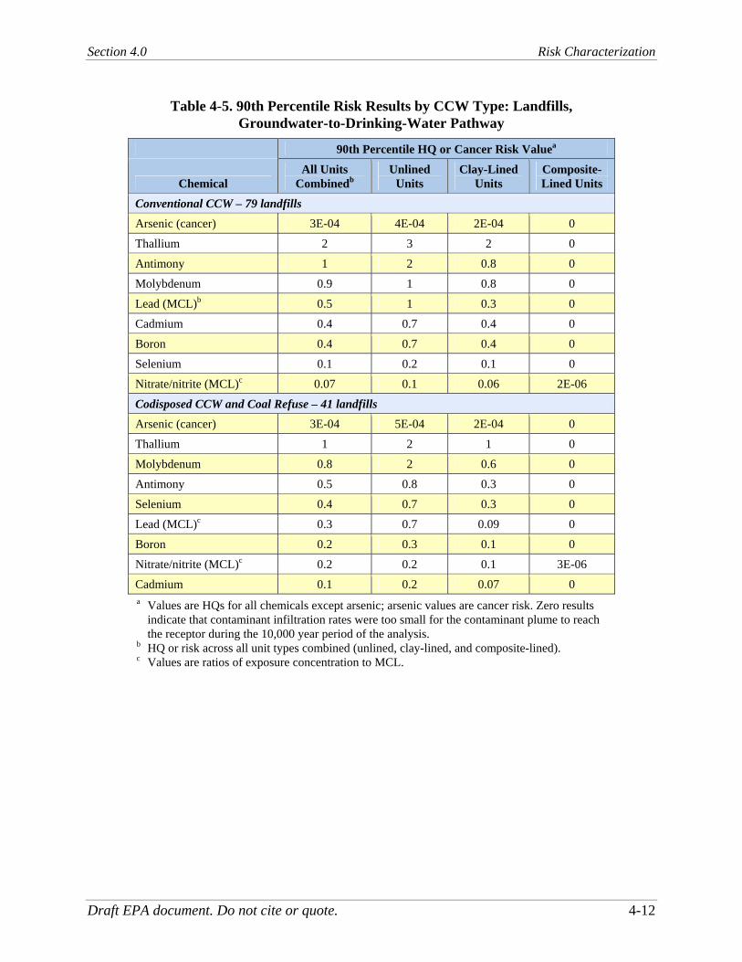
Section 4.0 Risk Characterization
Draft EPA document. Do not cite or quote. 4-12
Table 4-5. 90th Percentile Risk Results by CCW Type: Landfills, Groundwater-to-Drinking-Water Pathway
90th Percentile HQ or Cancer Risk Valuea
Chemical All Units
Combinedb Unlined
Units Clay-Lined
Units Composite-Lined Units
Conventional CCW – 79 landfills Arsenic (cancer) 3E-04 4E-04 2E-04 0
Thallium 2 3 2 0
Antimony 1 2 0.8 0
Molybdenum 0.9 1 0.8 0
Lead (MCL)b 0.5 1 0.3 0
Cadmium 0.4 0.7 0.4 0
Boron 0.4 0.7 0.4 0
Selenium 0.1 0.2 0.1 0
Nitrate/nitrite (MCL)c 0.07 0.1 0.06 2E-06
Codisposed CCW and Coal Refuse – 41 landfills Arsenic (cancer) 3E-04 5E-04 2E-04 0
Thallium 1 2 1 0
Molybdenum 0.8 2 0.6 0
Antimony 0.5 0.8 0.3 0
Selenium 0.4 0.7 0.3 0
Lead (MCL)c 0.3 0.7 0.09 0
Boron 0.2 0.3 0.1 0
Nitrate/nitrite (MCL)c 0.2 0.2 0.1 3E-06
Cadmium 0.1 0.2 0.07 0 a Values are HQs for all chemicals except arsenic; arsenic values are cancer risk. Zero results
indicate that contaminant infiltration rates were too small for the contaminant plume to reach the receptor during the 10,000 year period of the analysis.
b HQ or risk across all unit types combined (unlined, clay-lined, and composite-lined). c Values are ratios of exposure concentration to MCL.

Section 4.0 Risk Characterization
Draft EPA document. Do not cite or quote. 4-13
Table 4-6. 50th Percentile Risk Results by CCW Type: Landfills, Groundwater-to-Drinking-Water Pathway
50th Percentile HQ or Cancer Risk Valuea
Chemical All Units
Combinedb Unlined
Units Clay-Lined
Units Composite-Lined Units
Conventional CCW – 79 landfills Arsenic (cancer) 2E-06 6E-06 4E-06 0
Thallium 0.08 0.2 0.1 0
Antimony 0.02 0.04 0.02 0
Molybdenum 0.03 0.05 0.04 0
Lead (MCL)b 3E-08 4E-04 2E-08 0
Cadmium 0.005 0.01 0.008 0
Boron 0.007 0.01 0.01 0
Selenium 0.004 0.009 0.006 0
Nitrate/nitrite (MCL)c 0.002 0.004 0.003 0
Codisposed CCW and Coal Refuse – 41 landfills Arsenic (cancer) 4E-06 2E-05 6E-06 0
Thallium 0.06 0.2 0.07 0
Molybdenum 0.006 0.02 0.006 0
Antimony 0.01 0.05 0.02 0
Selenium 0.008 0.03 0.01 0
Lead (MCL)c 6E-07 0.01 2E-07 0
Boron 0.002 0.008 0.003 0
Nitrate/nitrite (MCL)c 0.01 0.04 0.009 0
Cadmium 0.003 0.02 0.004 0 a Values are HQs for all chemicals except arsenic; arsenic values are cancer risk. Zero results
indicate that contaminant infiltration rates were too small for the contaminant plume to reach the receptor during the 10,000 year period of the analysis.
b HQ or risk across all unit types combined (unlined, clay-lined, and composite-lined). c Values are ratios of exposure concentration to MCL.

Section 4.0 Risk Characterization
Draft EPA document. Do not cite or quote. 4-14
Table 4-7. 90th Percentile Risk Results by CCW Type: Surface Impoundments, Groundwater-to-Drinking-Water Pathway
90th Percentile HQ or Cancer Risk Valuea
Chemical All Units
Combinedb Unlined
Units Clay-Lined
Units Composite-Lined Units
Conventional CCW – 44 surface impoundments Arsenic (cancer) 1E-03
2E-03 9E-04 2E-07
Nitrate/nitrite (MCL)c 10 20 10 9E-04
Molybdenum 6 8 5 7E-03
Boron 5 7 4 5E-03
Selenium 2 2 1 1E-03
Lead (MCL)c 1 3 0.7 1E-21
Cadmium 0.4 0.5 0.3 4E-11
Cobalt 0.01 0.01 6E-03 0
Codisposed CCW and Coal Refuse – 72 surface impoundments Arsenic (cancer) 2E-02 2E-02 7E-03 4E-06
Cadmium 8 9 3 5E-05
Cobalt 7 8 3 4E-08
Lead (MCL)c 6 9 1 1E-19
Molybdenum 3 3 2 4E-03
Boron 1 1 0.5 2E-03
Selenium 0.8 0.8 0.4 1E-03
Nitrate/nitrite (MCL)c 0.3 0.4 0.2 1E-04 a Values are HQs for all chemicals except arsenic; arsenic values are cancer risk. Zero results
indicate that contaminant infiltration rates were too small for the contaminant plume to reach the receptor during the 10,000 year period of the analysis.
b HQ or risk across all unit types combined (unlined, clay-lined, and composite-lined). c Values are ratios of exposure concentration to MCL.

Section 4.0 Risk Characterization
Draft EPA document. Do not cite or quote. 4-15
Table 4-8. 50th Percentile Risk Results by CCW Type: Surface Impoundments, Groundwater-to-Drinking-Water Pathway
50th Percentile HQ or Cancer Risk Valuea
Chemical All Units
Combinedb Unlined
Units Clay-Lined
Units Composite–Lined Units
Conventional CCW – 44 surface impoundments Arsenic (cancer) 7E-05
1E-04 6E-05 0
Nitrate/nitrite (MCL)c 0.05 0.1 0.05 7E-08
Molybdenum 0.6 1.1 0.5 2E-11
Boron 0.2 0.4 0.2 3E-11
Selenium 0.07 0.1 0.07 2E-11
Lead (MCL)c 0.02 0.05 0.007 0
Cadmium 0.03 0.05 0.02 0
Cobalt 0.001 0.003 8E-04 0
Codisposed CCW and Coal Refuse – 72 surface impoundments Arsenic (cancer) 4E-04 6E-04 2E-04 0
Cadmium 0.1 0.1 0.05 0
Cobalt 0.3 0.4 0.09 0
Lead (MCL)c 0.09 0.1 0.01 0
Molybdenum 0.6 0.8 0.3 3E-18
Boron 0.1 0.1 0.06 5E-15
Selenium 0.08 0.1 0.03 5E-15
Nitrate/nitrite (MCL)c 0.02 0.03 0.01 4E-08 a Values are HQs for all chemicals except arsenic; arsenic values are cancer risk. Zero results
indicate that contaminant infiltration rates were too small for the contaminant plume to reach the receptor during the 10,000 year period of the analysis.
b HQ or risk across all unit types combined (unlined, clay-lined, and composite-lined). c Values are ratios of exposure concentration to MCL.
4.1.3.2 FBC Wastes
Tables 4-9 and 4-10 show the 90th- and 50th-percentile risk results for FBC landfills by unit type. At the 90th percentile in landfills, arsenic cancer risks are 3x10⁻⁵ for unlined units, 6x10⁻⁵ for clay-lined units, and 0 for composite-lined units. Noncancer hazard quotients exceed 1 for only thallium (4) and antimony (3) in clay-lined units. No risks exceeded the risk criteria at the 50th percentile. These results suggest lower risks than for conventional CCW and CCW codisposed with coal refuse. The difference may be attributed to lower FBC leachate concentrations and the alkaline nature of FBC waste.
Note that clay-lined FBC landfills show higher risks than unlined facilities, which is counterintuitive considering how clay-lined and unlined units are designed and operated. This

Section 4.0 Risk Characterization
Draft EPA document. Do not cite or quote. 4-16
result reflects the characteristics of the limited number and locations of FBC landfills5 and illustrates how the probabilistic analysis design and availability of facility data can impact risk results (and why FBC results are treated separately in the risk characterization). As presented in Section 3.1.2 and in Figure 3-2, the Monte Carlo analysis was designed to evaluate risks posed by current waste management practices for a given WMU type, waste type, and waste constituent. This approach limits the effects of data availability for the different liner configurations when the risks are aggregated over all units (lined and unlined) combined. However, when the risk results of an exposure pathway are viewed at a resolution finer than the analysis design, a small sample size for a particular waste and WMU type scenario (as occurs for FBC waste), along with the interactions of liner type with other site-based inputs (notably infiltration rate and the size of the WMU), can produce unexpected results. In the case of FBC wastes, the characteristics (primarily infiltration rate and areas) of the three unlined landfills were such that their risks were lower than the clay-lined FBC landfills.
Table 4-9. 90th Percentile Risk Results for FBC Wastes: Landfills, Groundwater-to-Drinking-Water Pathway
90th Percentile HQ or Cancer Risk Valuea
Chemical All Units
Combinedb Unlined
Units Clay-Lined
Units Composite-Lined Units
FBC Waste – 7 landfills Arsenic (Cancer) 4E-05
3E-05 6E-05 0
Thallium 2 1 4 0
Antimony 1 0.8 3 0
Lead (MCL)c 0.4 0.4 0.6 0
Molybdenum 0.3 0.2 0.5 0
Cadmium 0.2 0.1 0.3 0
Selenium 0.1 0.08 0.1 0
Nitrate/nitrite (MCL)c 0.05 0.03 0.07 5E-08
Boron 0.04 0.02 0.07 0 a Values are HQs for all chemicals except arsenic; arsenic values are cancer risk. Zero results
indicate that contaminant infiltration rates were too small for the contaminant plume to reach the receptor during the 10,000-year period of the analysis.
b HQ or risk across all unit types combined (unlined, clay-lined, and composite-lined). c Values are ratios of exposure concentration to MCL.
5 FBC WMU data were available for only seven landfills (3 unlined, 3 clay-lined, and 1 composite-lined), and it is
not known how representative these data are with respect to WMU characteristics and locations throughout the United States.

Section 4.0 Risk Characterization
Draft EPA document. Do not cite or quote. 4-17
Table 4-10. 50th Percentile Risk Results for FBC Wastes: Landfills, Groundwater-to-Drinking-Water Pathway
50th Percentile HQ or Cancer Risk Valuea
Chemical All Units
Combinedb Unlined
Units Clay-Lined
Units Composite-Lined Units
FBC Waste – 7 landfills Arsenic (Cancer) 0
0 4E-07 0
Thallium 0.008 0 0.2 0
Antimony 0.002 0 0.09 0
Lead (MCL)c 0 0 2E-04 0
Molybdenum 0.003 0 0.04 0
Cadmium 4E-07 0 0.01 0
Selenium 3E-04 0 0.01 0
Nitrate/nitrite (MCL)c 1E-04 3E-08 0.004 0
Boron 2E-04 0 0.003 0 a Values are HQs for all chemicals except arsenic; arsenic values are cancer risk. Zero results
indicate that contaminant infiltration rates were too small for the contaminant plume to reach the receptor during the 10,000-year period of the analysis.
b HQ or risk across all unit types combined (unlined, clay-lined, and composite-lined). c Values are ratios of exposure concentration to MCL.
4.1.4 Results by Unit Type
The effect of unit type on human health risk for the groundwater-to-drinking-water pathway can be seen in Tables 4-1 and 4-2, which compare 90th and 50th percentile risks, respectively, for WMUs that are unlined, clay lined, and lined with composite liners from the 1995 EPRI survey data (EPRI, 1997). At the 90th percentile, lined units produced lower risk estimates than unlined units for all constituents modeled. Composite liners produced very low to zero risk estimates as compared to clay liners for all constituents modeled for both landfills and surface impoundments. For surface impoundments, clay liners produced higher risk estimates for all constituents as compared to clay liners in landfills. Similar trends are evident at the 50th percentile, where composite liners produced risk estimates of zero or near zero for all constituents for surface impoundments.
Table 4-11 shows the frequency of each of the unit types in the 1995 EPRI survey data modeled in this analysis, and it compares these data with the unit type frequency in the more recent DOE/EPA study (U.S. DOE, 2006). The 56 WMUs surveyed in the U.S. DOE 2006 study were commissioned between 1994 and 2004. Although the actual number of WMUs that were established in that timeframe cannot be verified, based on proxy data (i.e., CCW available for disposal in those states with identified, new WMUs and coal-fired power plant generating capacity), the sample coverage is estimated to be at least between 61 and 63 percent of the total

Section 4.0 Risk Characterization
Draft EPA document. Do not cite or quote. 4-18
population of the newly commissioned WMUs.6 With the exception of one landfill, the newly constructed facilities are all lined, with either clay, synthetic, or composite liners. The single unlined landfill identified in the recent DOE report receives bottom ash, which is characterized as an inert waste by the state, and therefore, a liner is not required. As Table 4-11 shows, there is a marked trend away from unlined WMUs in favor of lined units, with a distinct preference for synthetic or composite liners. Comparison of the 26 coal combustion plants in both the EPRI survey and the DOE/EPA survey (U.S. DOE, 2006) shows that although most of those facilities (17 of 26) were using unlined WMUs in 1995, all 26 are now placing wastes in new or expanded landfills or surface impoundments that are lined with clay, synthetic, or composite liners. However, it is likely that the older unlined units were closed with wastes in place, and that these wastes therefore still pose a threat through groundwater pathways. Also, the number of unlined unit that continue to operate in the United States cannot be determined from the available data.
Table 4-11. Unit Types in EPRI Survey
Liner Type Landfills Surface
Impoundments 1995 EPRI Surveya – 181 facilities Unlined 40% 68% Compacted clay 45% 27% Synthetic or composite (clay and synthetic) 16% 5%
Total 100% 100% 2004 DOE Surveyb – 56 Facilities Unlined 3% 0% Compacted clay 29% 17% Synthetic or composite (clay and synthetic) 68% 83%
Total 100% 100% a EPRI (1997) b U.S.DOE (2006)
As described in Sections 3.2.1 and 3.3.1, the characteristics of the liners used in the CCW risk were taken from the IWEM model as representative of the general performance of each liner type. For landfills, an engineered compacted clay liner (3 feet thick, with a hydraulic conductivity of 1 x 10⁻⁷ cm/s) reduced the 90th percentile risk by a factor of about 2 to 4 compared to no liner, but did not change the constituents at or above the risk criteria (arsenic and thallium). For surface impoundments, clay liners did reduce the risk to just below the risk criteria for cobalt, lead, and selenium.
Composite (clay and synthetic) liners, as modeled in this risk assessment (see Sections 3.2 and 3.3), were much more effective at reducing risk for all constituents; 90th (and
6 For additional details as to how these estimates were derived, the reader is referred to the DOE study, pages S-2 –
S-3 of the Summary Section and Section 3.1.2..

Section 4.0 Risk Characterization
Draft EPA document. Do not cite or quote. 4-19
50th) percentile risks with composite liners for landfills were zero7 for arsenic and metals and
very low or zero for nitrate/nitrite, and were well below the risk criteria for all constituents for surface impoundments. The analysis used data collected for composite liner performance at industrial waste management facilities, including liner leakage rate for landfills and the number of liner perforations for surface impoundments (TetraTech, 2001). Because data on CCW liner leakage rates are not available, there is some uncertainty in applying these Industrial D liner performance data to CCW disposal units. Still, these rates do reflect actual performance data from liners under real WMUs, and they demonstrate that composite liners can be effective in reducing leaching from CCW WMUs and suggest that there will be a significant decrease in risk from CCW disposal if more facilities line their WMUs with composite liners. Information from the more recent DOE/EPA study (U.S. DOE, 2006) indicates that composite liners are much more prevalent in newly constructed facilities, so the risks from CCW disposal should be lower for newer CCW landfills and surface impoundments.
4.1.5 Constituents Not Modeled in the Full-Scale Assessment
As described in Section 2.1.1.2, resources did not allow full-scale modeling to be conducted for all 21 constituents that were above the screening criteria in the initial screening analysis; nine constituents that were judged to likely have generally lower risks to human health and ecological risks were not modeled in the full-scale risk assessment.8 Five of these chemicals (chromium, fluoride, manganese, vanadium, and nickel) had drinking water pathway HQs in the screening analysis ranging from 1 to less than 6 for surface impoundments, and three (chromium, fluoride, and vanadium) had screening HQs of 2 for landfills.
To address these constituents, we developed surrogate risk attenuation factors by dividing the screening risk results by the full-scale risk results, across all unit types combined, for the constituents modeled in the full-scale assessment. This comparison was done only for the drinking water exposure pathway, the only human health exposure pathway for which the risks for these constituents were above the screening criteria. Table 4-12 shows the risk attenuation factor statistics for the modeled constituents, and Table 4-13 shows the results of applying the median and 10th percentile attenuation factors to the screening risk results for the marginal constituents. Differences in attenuation among the modeled constituents reflects differences in contaminant sorption and mobility. The 10th percentile attenuation factor was selected as a conservative value representing the more mobile constituents, such as arsenic, selenium, and molybdenum. The 50th percentile (or median) risk represents a central tendency value.
For landfills, the risk attenuation factors ranged from 6 to 40, with the lower attenuation factors mainly representing the more mobile constituents (i.e., those with lower soil sorption potential). Both the median and 10th percentile risk attenuation factors were adequate to reduce risks for all nine constituents below an HQ of 1.
7 The absence of risk indicates that contaminant infiltration rates were too small for the contaminant plume to reach
the receptor well during the 10,000 year period of the analysis. See Section 3.2.2 for a discussion of the empirical liner infiltration data used in this analysis.
8 These constituents of marginal concern had no human health HQs greater than 6 and only one or no ecological HQs greater than 100.

Section 4.0 Risk Characterization
Draft EPA document. Do not cite or quote. 4-20
For surface impoundments, risk attenuation factors were considerably lower, ranging from 1 to 9, reflecting higher contaminant mobility due to the higher hydraulic head in surface impoundments (as compared to landfills) and a lower proportion of liners. For the same reason, the screening HQs for surface impoundments were higher than the landfill HQs. As a result of this combination of higher HQs and lower risk attenuation factors, only the HQ for nickel was reduced to below 1 by applying the attenuation factors. The other constituents (chromium, fluoride, manganese, and vanadium) still show risks slightly above the risk criteria, with HQs ranging from 1.4 to 3.5. This is consistent with the general trend in this analysis of surface impoundments showing higher risks and more risks exceeding the risk criteria than CCW landfills.
Table 4-12. Risk Attenuation Factora Statistics for Modeled Constituents— Groundwater to Drinking Water Pathway
Statistic Landfill Surface Impoundment 10th percentile 7 1.6 50th percentile 12 2.6 Average 16 3.3 Maximum 40 9.3 Number of data points 9 8
a The risk attenuation factor is the ratio of the full-scale analysis risk and screening analysis risk for a constituent modeled in the full-scale analysis.
Table 4-13. Summary of Risk Results for Constituents Using Risk Attenuation Factors—Groundwater-to-Drinking-Water Pathway
Landfill Surface Impoundment
WMU/Pathway Screening
HQ
HQ with Median
Attenuation
HQ with 10th
Percentile Attenuation
Screening HQ
HQ with Median
Attenuation
HQ with 10th
Percentile Attenuation
Chromium VI 2.3 0.2 0.3 4.2 1.6 2.6
Fluoride 1.8 0.2 0.3 5.2 2.0 3.3
Manganese 1 0.1 0.1 5.6 2.2 3.5
Vanadium 2.2 0.2 0.3 2.3 0.9 1.4
Nickel - - - 1.3 0.5 0.8

Section 4.0 Risk Characterization
Draft EPA document. Do not cite or quote. 4-21
4.2 Ecological Risks
EPA defines ecological risk characterization in terms of (1) the risk estimation, which integrates the exposure and stressor-response profile to estimate the likelihood of adverse ecological effects and (2) the risk description, which synthesizes the overall conclusion of the assessment and addresses assumptions, uncertainty, and limitations.
For assessments that are based on a HQ approach, as this one is, the comparison of modeled exposure concentrations to CSCLs to estimate risk has a binary outcome: either the constituent concentration is above the environmental quality criteria (HQ greater than 1) or the concentration is below the criteria (HQ less than or equal to 1). For the full-scale analysis, an ecological HQ greater than 1 was selected by EPA as a criterion for decision making. Because the CSCLs were based on de minimis ecological effects, it is generally presumed that an HQ at or below 1 indicates a low potential for adverse ecological effects for those receptors included in the analysis for which data are available. However, it is important to recognize that although this method provides important insight into the potential for adverse ecological effects, the results are relevant only to those receptors that were included in the assessment and for which data were available. The results have limited utility in interpreting the ecological significance of predicted effects, and caution should be exercised in extrapolating to ecosystems (e.g., wetlands) and receptors (e.g., threatened and endangered species) not explicitly modeled.
This section presents risk results for the two groundwater-to-surface-water ecological exposure pathways investigated in the full-scale analysis: (1) receptors exposed to CCW constituents in the water column (surface water receptors) and (2) receptors exposed to CCW constituents in bed sediment (sediment receptors). Results are presented for the two WMU types addressed in the analysis: landfills and surface impoundments. The ecological risk results are presented for all unit types combined and were not broken out separately for the different unit types.
The ecological risk results suggest the potential for adverse ecological effects to aquatic systems from CCW releases into the subsurface and subsequent connection with surface waters, particularly for CCW managed in unlined surface impoundments. As with human health risks, the higher prevalence of liners in newer facilities should result in lower risks in current and future CCW disposal facilities than those presented in this risk assessment.
4.2.1 Surface Water Receptors
Table 4-14 presents the 90th and 50th percentile results for the groundwater-to-surface-water pathway for surface water receptors for landfills and surface impoundments. For landfills, only boron (200) and lead (4) show HQs above the risk criteria at the 90th percentile. For surface impoundments, boron (2000), lead (20), arsenic (10), selenium (10), cobalt (5), and barium (2) showed 90th percentile risks above the risk criteria. The 50th percentile results are well below an HQ of 1 for landfills and only exceed an HQ of 1 for boron (4) in surface impoundments.
The difference in the number and magnitude of HQs that exceed the risk criterion between landfills and surface impoundments is likely the result of higher CCW constituent concentrations in surface impoundment porewater and the greater flux of contaminants to

Section 4.0 Risk Characterization
Draft EPA document. Do not cite or quote. 4-22
groundwater predicted during the active life of the surface impoundment. As discussed in Section 4.1, the higher infiltration rates for surface impoundments result from a higher hydraulic head in the impoundment and a higher proportion of unlined surface impoundments than landfills.
Table 4-14. Summary of Full-Scale CCW Ecological Risk Results: Groundwater-to-Surface-Water Pathway, Aquatic Receptorsa
Chemical 90th Percentile
HQ 50th Percentile
HQ Pathway Receptor Landfills Boron 200 0.04 direct contact aquatic biota Lead 4 2E-08 ingestion river otter Selenium 1 3E-04 direct contact aquatic biota Arsenic 0.7 9E-10 direct contact aquatic biota Barium 0.8 3E-18 direct contact aquatic biota Cadmium 0.3 3E-05 direct contact aquatic biota Aluminum 0.008 1E-09 direct contact aquatic biota Surface Impoundments Boron 2000 4 direct contact aquatic biota Lead 20 0.02 ingestion river otter Arsenic 10 0.01 direct contact aquatic biota Selenium 10 0.02 direct contact aquatic biota Cobalt 5 0.007 direct contact aquatic biota Barium 2 0.003 direct contact aquatic biota Cadmium 1 0.004 direct contact aquatic biota Aluminum 0.02 0.0003 direct contact aquatic biota a Zero results indicate that contaminant infiltration rates were too small for the
contaminant plume to reach the receptor during the 10,000 year period of the analysis.
4.2.2 Sediment Receptors
Table 4-15 presents the 90th and 50th percentile results of the ground-water-to-surface-water pathway for sediment receptors for landfills and surface impoundments. For landfills, lead, (20), arsenic (6), and cadmium (2) show 90th percentile risks above the risk criteria. For surface impoundments, lead (200), arsenic (100), and cadmium (20) showed 90th percentile risks above the risk criteria. Although cadmium was not above the risk criterion in surface water, it did have an HQ of 20 in sediments at the 90th percentile. None of the constituents modeled showed sediment risks at or above the risk criteria at the 50th percentile.

Section 4.0 Risk Characterization
Draft EPA document. Do not cite or quote. 4-23
Table 4-15. Summary of Full-Scale CCW Ecological Risk Results: Groundwater-to-Surface-Water Pathway, Sediment Receptorsa
Chemical 90th Percentile
HQ 50th Percentile
HQ Pathway Receptor
Landfills Lead 20 3E-08 ingestion spotted sandpiper Arsenic 6 7E-04 ingestion spotted sandpiper Cadmium 2 6E-05 direct contact sediment biota Antimony 0.9 4E-05 direct contact sediment biota Molybdenum 0.05 1E-05 ingestion spotted sandpiper Barium 0.002 6E-21 ingestion spotted sandpiper Surface Impoundments Lead 200 0.05 ingestion spotted sandpiper Arsenic 100 0.2 ingestion spotted sandpiper Cadmium 20 0.009 direct contact sediment biota Molybdenum 0.7 0.002 ingestion spotted sandpiper Barium 0.007 8E-06 ingestion spotted sandpiper a Zero results indicate that contaminant infiltration rates were too small for the contaminant
plume to reach the receptor during the 10,000 year period of the analysis.
4.2.3 Constituents Not Modeled in the Full-Scale Assessment
As described in Section 2.1.1.2, resources did not allow full-scale modeling to be conducted for 6 constituents with generally lower risks to ecological receptors.9 These chemicals (chromium, vanadium, beryllium, copper, silver, and zinc), had surface water pathway HQs in the screening analysis ranging from 16 to 110 for landfills, and four (chromium, vanadium, copper, and silver) had screening HQs ranging from 14 to 33 for surface impoundments.
These constituents were addressed using risk attenuation factors developed by dividing the screening risk results by the full-scale risk results for the constituents modeled in the full-scale assessment. Tables 4-16 and 4-17 show the results of this comparison for the surface water ecological risk exposure pathway. Table 4-16 shows the risk attenuation factors for the modeled constituents, and Table 4-17 shows the results of applying the median (central tendency) and 10th percentile (conservative) attenuation factors to the screening risk results for constituents that were not modeled.
For landfills, the risk attenuation factors ranged from 50 to 2,000. Both the median and 10th percentile risk attenuation factors were adequate to reduce risks to an HQ below 1 for all constituents except for silver. Although silver shows an HQ of 1.5 using the 10th percentile
9 These constituents had only one or no ecological HQs greater than 100.

Section 4.0 Risk Characterization
Draft EPA document. Do not cite or quote. 4-24
attenuation factor, silver’s low mobility would probably result in a higher attenuation factor (i.e., at the median or greater).
For surface impoundments, risk attenuation factors ranged from 7 to 64, reflecting higher contaminant mobility from the higher hydraulic head in the surface impoundments and a lower prevalence of liners (compared to landfills). HQs were reduced below 1 for all four unmodeled constituents with the median attenuation factor (38), and the HQ for silver was reduced to 0.8 by applying the 10th percentile attenuation factor (17). The other three constituents (chromium, vanadium, and copper) show risks only slightly above the risk criteria with the10th percentile attenuation (HQs ranging from 1.4 to 1.9). It is unlikely that these results represent true risks above the risk criteria: vanadium and copper are likely less mobile than the 10th percentile attenuation factor reflects (thus the true risk is likely lower), and the risks for chromium are based on the highly conservative assumption of 100 percent hexavalent chromium.
Table 4-16. Risk Attenuation Factora Statistics for Modeled Constituents— Ecological Risk, Surface Water Pathway
Statistic Landfill Surface Impoundment 10th percentile 75 17 50th percentile 178 38 Average 483 38 Maximum 2,000 64 Number of data points 6 7 a The risk attenuation factor is the ratio of the full-scale analysis risk and screening
analysis risk for a constituent modeled in the full-scale analysis.
Table 4-17. Summary of Risk Results Using Risk Attenuation Factors— Ecological Risk, Surface Water Pathway
Landfill Surface Impoundment
WMU/Pathway Screening
HQ
HQ with Median
Attenuation
HQ with 10th Percentile
Attenuation Screening
HQ
HQ with Median
Attenuation
HQ with 10th Percentile
Attenuation
Chromium VI 18 0.1 0.2 33 0.9 1.9
Vanadium 23 0.1 0.3 24 0.6 1.4
Beryllium 24 0.1 0.3 - - -
Copper 16 0.09 0.2 31 0.8 1.8
Silver 110 0.6 1.5 14 0.4 0.8
Zinc 16 0.09 0.2 - - -

Section 4.0 Risk Characterization
Draft EPA document. Do not cite or quote. 4-25
4.3 Sensitivity Analysis
EPA conducted a sensitivity analysis on the probabilistic risk assessment to determine which model inputs were most important to risk, which in turn will help focus additional analyses or data collection efforts on the most important drivers of risk, and help identify the important factors to consider when evaluating regulatory and management options for CCW. The sensitivity analysis also can help identify parameters that are both sensitive and highly uncertain, which affects the confidence in the results. This sensitivity analysis used a response-surface regression method that derives a statistical model for risk (as the dependent variable) based on the input parameters from the probabilistic analysis (as independent variables).
Environmental concentration (rather than risk) was chosen as the dependent variable for the sensitivity analysis because (1) there is a direct, linear relationship between environmental concentrations and risks and (2) the additional inputs used to calculate risk from environmental concentration (i.e., exposure factors, such as body weight, ingestion rates) are lifestyle variables that are not amenable to regulation to reduce or manage risk. Furthermore, these variables have well-established, peer-reviewed, national distributions, which are regularly used in the probabilistic national risk analyses conducted by EPA. Therefore, the contribution of the exposure factors to the variability in risk is not particularly useful for the purposes of the sensitivity analysis: to help direct additional analyses in support of developing CCW regulatory options, to help focus any future data collection efforts on the most sensitive variables, or to better understand sources of uncertainty in the CCW risk results.
The outputs from the sensitivity analysis are the goodness-of-fit values for the regression models and the relative importance of each input parameter in determining environmental concentrations across different WMU, waste type, and constituent scenarios. The goodness-of-fit values of the regression models were moderate to very good for the drinking water pathway (R2=0.53–0.90) and good to very good for fish consumption (R2=0.76–0.90). In general, the drinking water pathway had a larger number of input parameters that were significant (seven) than the fish consumption pathway (three). The most sensitive parameters for most (over 75 percent) of the drinking water scenarios10 evaluated were parameters impacting groundwater flow:
Infiltration rate within the WMU footprint
Leachate concentration from the WMU
Aquifer hydraulic conductivity and gradient (i.e., groundwater velocity).
For strongly sorbing contaminants (i.e., metals with high soil/water partition coefficients), sorption and travel time parameters become more important, including
Adsorption isotherm coefficient
Depth to groundwater
Receptor well distance.
10 Scenarios represent unique combinations of WMU, waste type, chemical, exposure pathway, and receptor.

Section 4.0 Risk Characterization
Draft EPA document. Do not cite or quote. 4-26
For the fish consumption pathway, only three variables were consistently significant across scenarios:
Infiltration rate within the WMU footprint
Leachate concentration from the WMU
Waterbody flow rate.
Additional detail on how the CCW sensitivity analysis was conducted can be found in U.S. EPA (2005). In terms of the model inputs, the sensitivity analysis found that the most consistent drivers of the risk results are constituent concentration in waste leachate (i.e., the source term for the risk assessment and infiltration rate through the WMU), which is largely controlled by the liner conditions and, to a lesser extent, soil type and (for landfills only) precipitation. These variables and their uncertainties are discussed in the following section.
4.4 Variability and Uncertainty
Variability and uncertainty are different conceptually in their relevance to a probabilistic risk assessment. Variability represents true heterogeneity in characteristics, such as body weight differences within a population or differences in pollutant levels in the environment. It accounts for the distribution of risk within the exposed population. Although variability may be known with great certainty (e.g., age distribution of a population may be known and represented by the mean age and its standard deviation), it cannot be eliminated and needs to be treated explicitly in the assessment. Uncertainty is a description of the imperfection in knowledge of the true value of a particular parameter. In contrast to variability, uncertainty can be reduced through additional information-gathering or analysis (i.e., better data, better models). EPA typically classifies the major areas of uncertainty in risk assessments as scenario uncertainty, model uncertainty, and parameter uncertainty. Scenario uncertainty refers to missing or incomplete information needed to fully define exposure and dose. Model uncertainty is a measure of how well the model simulates reality. Parameter uncertainty is the lack of knowledge regarding the true value of a parameter used in the assessment.
Uncertainty and variability can be addressed two ways:
By varying parameter values in a probabilistic assessment such as a Monte Carlo analysis
By comparing the data or results to other data or other studies such as damage cases or alternative results based on different assumptions.
In planning this assessment, we addressed as much of the variability as possible, either directly in the Monte Carlo analysis or through aggregation of the data into discrete elements of the analysis. For example, spatial variability in soil, aquifer, and climate data is accounted for by using distributions for soil and aquifer properties around the facility when the actual
Variability arises from true heterogeneity in characteristics, such as body weight differences within a population or differences in contaminant levels in the environment. Uncertainty represents a lack of knowledge about factors such as the nature of adverse effects from exposure to constituents, which may be reduced with additional research to improve data or models.
Section 4.0 Risk Characterization
Draft EPA document. Do not cite or quote. 4-27
environmental characteristics around a WMU are uncertain. Conversely, variability in waste leachate concentrations was represented by a national database of CCW constituent concentrations from disposal sites around the country. These data were aggregated by waste and WMU types that were defined by statistically significant differences in concentration. Variability in human exposure factors (e.g., body weight, ingestion rates) was accounted for using national distributions that represent the range of possible values.
Because CCW is generated nationwide, its disposal may occur anywhere in the United States. Thus, this assessment characterized environmental conditions that influence the fate and transport of constituents in the environment using site-specific data collected around coal-fired power plants with onsite CCW disposal facilities. Spatial variability in environmental setting was accounted for by the site-to-site variables for the 181 CCW disposal sites modeled in the analysis using 41 different climate regions and 9 different resources regions throughout the contiguous 48 states.
In summary, a distribution of exposures was developed that includes specific consideration of the variability in the following sensitive model parameters
WMU characteristics, in particular liner type (which strongly influences infiltration rate)
CCW constituent concentrations in waste leachate
Distance to nearest well
Site-specific environmental conditions (especially groundwater flow conditions)
Human exposure factors.
Uncertainty also was considered in the analysis by using reasonable ranges and distributions when variables were not known exactly. For example, when a soil texture or groundwater flow conditions could not be precisely assigned at a site, multiple soil types or hydrogeologic environments would be sampled based on the soil and aquifer types that are likely to be present at the site.
The treatment of variability and uncertainty in model parameters using a Monte Carlo simulation forms the basis for the national exposure distributions used in this analysis to estimate risk. Previous sections of this document describe how we generated distributions and estimated input parameter values and then used these values in models to estimate risk. The discussion in this section focuses on how this treatment of variability and uncertainty affects the analysis results and on various comparisons we performed on the results or critical input data to evaluate uncertainty.
4.4.1 Scenario Uncertainty
Sources of scenario uncertainty include the assumptions and modeling decisions that are made to represent an exposure scenario. Because this risk assessment attempts to characterize current conditions by estimating risks from actual CCW disposal sites across the country, it is subject to less scenario uncertainty than risk assessments that rely on hypothetical conceptual models. However, certain aspects of the scenario are uncertain.

Section 4.0 Risk Characterization
Draft EPA document. Do not cite or quote. 4-28
CCW Management Unit Data. The landfills and surface impoundments modeled in this risk assessment were placed, sized, and lined according to data from the 1995 EPRI survey (EPRI, 1997). New data collected by EPA and DOE since this risk assessment was conducted (U.S. DOE, 2006) indicate that liners are much more prevalent in WMUs constructed or expanded from 1994 through 2004 than in units in place before that. This suggests that the risks may be lower for future CCW disposal facilities (although most of the unlined WMUs have been closed with wastes remaining in the units).
Liner-related questions are especially important because liner configurations greatly influence infiltration rates, one of the most sensitive parameters in the risk assessment. In terms of risks through groundwater pathways, this risk assessment has shown that liners, in particular composite (combined clay and synthetic) liners, can limit risks through subsurface exposure pathway, and the DOE/EPA survey shows that liners are more prevalent in newly constructed WMUs and WMU expansions. Although the DOE/EPA survey does not shed light on how many unlined facilities are still operating today, it does indicate that more units are lined today than were in the 1995 EPRI survey data set on which this risk assessment is based.
Receptor Populations Evaluated. The human receptors evaluated for the CCW risk analysis are a family with children residing near the CCW disposal facility, drinking from a private well screened in a surficial aquifer or eating fish caught from a nearby stream or lake impacted by CCW leachate. Additionally, except for a 15-day vacation, it is assumed that adults and children are exposed daily and that the private well is the only source of drinking water. Although it is possible for other types of individuals to be exposed, the use of the resident adult and child as protective of other receptors and pathways is a conservative, simplifying assumption of the analysis. The lack of information to define and model actual exposure conditions also introduces uncertainty into this assessment, but EPA believes that the national distribution of exposure factors used is appropriate for a national assessment.
Additive Risks Across Pathways. The human receptors evaluated in the CCW risk assessment are assumed not to consume both contaminated fish and drinking water. Although this could potentially miss some higher exposures for a maximally exposed individual, analysis of the individual pathway results does not indicate that adding such risks would significantly change the conclusions of this risk assessment in terms of the constituents and exceeding the risk criteria.
Co-Occurrence of Ecological Receptors and Constituents. As a simplification for national-scale analyses in the absence of site-based data, co-occurrence of the ecological receptors and the constituents of concern is typically assumed. However, the prior probability that a receptor will be found in waterbodies affected by constituent releases from CCW WMUs is not known, nor is it known whether a receptor will forage for food in contaminated areas or if those areas do, in fact, support the type of habitat needed by the receptor. Although the assumption of co-occurrence was necessary for this analysis, relatively few field studies are available to demonstrate the relationship between adverse ecological effects and constituent releases from CCW as it is currently managed.

Section 4.0 Risk Characterization
Draft EPA document. Do not cite or quote. 4-29
Ecosystems and Receptors at Risk. One of the most intractable problems in conducting a predictive ecological risk assessment intended to reflect risks at a national scale is evaluating all of the receptors and ecosystems at risk. In Wastes from the Combustion of Coal by Electric Utility Power Plants - Report to Congress (U.S. EPA, 1988b), the authors pointed out that plants or animals of concern were located within a 5-km radius of the CCW WMUs at 12 to 32 percent of the sites. Although these figures are of limited spatial resolution, they suggest the possibility that threatened and endangered species or critical habitats may be at risk from CCW constituents. Examples of other critical assessment endpoints not evaluated in this analysis include the following:
Managed Lands: Because ecosystem degradation is proceeding at an unprecedented rate, and because protected lands play a critical role in preserving plant and animal species, managed areas in the United States represent well-recognized ecological values. Managed lands refer to a variety of lands designated by the federal government as worthy of protection, including National Wildlife Refuges, National Forests, Wilderness areas, and National Recreation areas.
Critical Habitats: Although critical habitats may be defined in a number of ways (e.g., presence of threatened species, decreasing habitat area), wetlands are widely recognized as serving critical ecological functions (e.g., maintenance of water quality). The U.S. Fish and Wildlife Service estimates that approximately 45 percent of the Nation’s threatened and endangered species directly depend on aquatic and wetland habitats. Consequently, impacts of chemical stressors on wetland habitats may have high ecological (and societal) significance. The presence of critical habitats such as wetlands is also used to inform the selection of ecological receptors (e.g., amphibians, waterfowl) and the construction of appropriate food webs.
Threatened and Endangered Species: For most ecological risk assessments of chemical stressors, available data on toxicity and biological uptake are sufficient to support the evaluation of effects on representative species populations or generalized communities (e.g., aquatic community). However, despite their obvious value, threatened and endangered species are frequently excluded from the analytical framework for national rulemakings. The assessment of threatened and endangered species requires a site-based approach in which locations, habitats, and species of concern are identified and characterized with respect to the spatial scale of constituent releases.
4.4.2 Model Uncertainty
Model uncertainty is associated with all models used in a risk assessment because models and their mathematical expressions are simplifications of reality that are used to approximate real-world conditions and processes and their relationships. Computer models are simplifications of reality, requiring exclusion of some variables that influence predictions but that cannot be included in models either because of their complexity or because data are lacking on a particular parameter. Models do not include all parameters or equations necessary to express reality because of the inherent complexity of the natural environment and the lack of sufficient data to describe the natural environment. Because this is a probabilistic assessment that predicts what may occur with the management of CCW under actual scenarios, it is possible to compare the results of these models to specific situations.

Section 4.0 Risk Characterization
Draft EPA document. Do not cite or quote. 4-30
The risk assessor needs to consider the importance of excluded variables on a case-by-case basis because a given variable may be important in some instances and not important in others. A similar problem can occur when a model that is applicable under one set of conditions is used for a different set of conditions. In addition, in some instances, choosing the correct model form is difficult when conflicting theories seem to explain a phenomenon equally well. In other instances, EPA does not have established model forms from which to choose to address certain phenomena, such as facilitated groundwater transport.
Models used in this analysis were selected based on science, policy, and professional judgment. These models were selected because they provide the information needed for this assessment and because they are generally considered to reflect the state of the science. Even though the models used in this analysis are used widely and have been accepted for numerous applications, they each retain significant sources of uncertainty. These limitations are well documented in the model development references cited in Section 3.
Although the sources of model uncertainty in this assessment could result in either an overestimation or an underestimation of risk, the models employed in this assessment have been developed over many years to support regulatory applications. As a result they have been designed to be protective towards the impacted populations that they represent. In other words, where simplifying assumptions are necessary, the assumptions are made in a way that will not underestimate risk.
Arsenic Speciation. Because the models used in this assessment do not speciate metals during soil or groundwater transport, arsenic speciation in the subsurface is a significant groundwater modeling uncertainty in this analysis. Arsenic can occur in either a +3 (arsenic III) or +5 (arsenic V) oxidation state in groundwater, with arsenic III being the more mobile form. Because the soil and groundwater models assume one form for each model run, the risk results presented for arsenic are based on arsenic III, which is a conservative, protective assumption (i.e., arsenic III has higher risks than arsenic V). Although arsenic is generally thought to occur in the +3 form in leachate, there is evidence from damage cases at CCW disposal sites that suggests that arsenic III is rapidly converted to arsenic V during subsurface transport, with the result that drinking water standards are rarely exceeded in offsite groundwater in spite of high landfill leachate concentrations (see, for example, U.S. EPA, 2000; U.S. EPA, 2003e; Lang and Schlictmann, 2004; Zillmer and Fauble, 2004). To address this uncertainty (i.e., how much an arsenic III assumption might overpredict offsite well concentrations) the models were run assuming arsenic V as the arsenic species in soil and groundwater. Figure 4-4 compares the risk results for arsenic III and arsenic V. Arsenic V has lower risks than arsenic III by about a factor of two, but the 90th percentile risks are still above risk criteria.
Bioavailability of Constituents to Ecological Receptors. For the purposes of this analysis, the model assumes that all forms of a constituent are equally bioavailable to ecological receptors, and therefore, the actual exposures that may occur in the field tend to be overestimated, thus making this a protective assumption. Both the chemical form and the environmental conditions influence bioavailability and ultimately the expression of adverse effects. For example, as discussed above, the form of arsenic has been shown to profoundly influence mobility and toxicity.
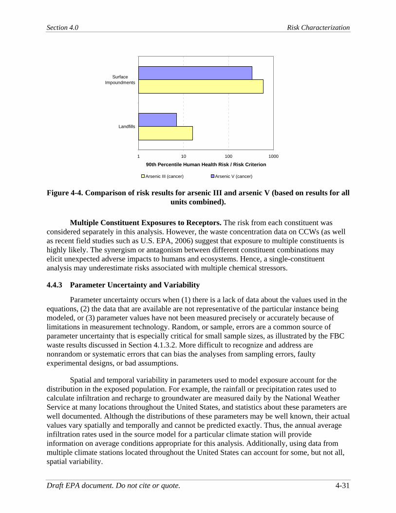
Section 4.0 Risk Characterization
Draft EPA document. Do not cite or quote. 4-31
1 10 100 1000
Landfills
SurfaceImpoundments
90th Percentile Human Health Risk / Risk Criterion
Arsenic III (cancer) Arsenic V (cancer)
Figure 4-4. Comparison of risk results for arsenic III and arsenic V (based on results for all units combined).
Multiple Constituent Exposures to Receptors. The risk from each constituent was considered separately in this analysis. However, the waste concentration data on CCWs (as well as recent field studies such as U.S. EPA, 2006) suggest that exposure to multiple constituents is highly likely. The synergism or antagonism between different constituent combinations may elicit unexpected adverse impacts to humans and ecosystems. Hence, a single-constituent analysis may underestimate risks associated with multiple chemical stressors.
4.4.3 Parameter Uncertainty and Variability
Parameter uncertainty occurs when (1) there is a lack of data about the values used in the equations, (2) the data that are available are not representative of the particular instance being modeled, or (3) parameter values have not been measured precisely or accurately because of limitations in measurement technology. Random, or sample, errors are a common source of parameter uncertainty that is especially critical for small sample sizes, as illustrated by the FBC waste results discussed in Section 4.1.3.2. More difficult to recognize and address are nonrandom or systematic errors that can bias the analyses from sampling errors, faulty experimental designs, or bad assumptions.
Spatial and temporal variability in parameters used to model exposure account for the distribution in the exposed population. For example, the rainfall or precipitation rates used to calculate infiltration and recharge to groundwater are measured daily by the National Weather Service at many locations throughout the United States, and statistics about these parameters are well documented. Although the distributions of these parameters may be well known, their actual values vary spatially and temporally and cannot be predicted exactly. Thus, the annual average infiltration rates used in the source model for a particular climate station will provide information on average conditions appropriate for this analysis. Additionally, using data from multiple climate stations located throughout the United States can account for some, but not all, spatial variability.

Section 4.0 Risk Characterization
Draft EPA document. Do not cite or quote. 4-32
4.4.3.1 Waste Concentrations
The CCW constituent database used to represent CCW total waste and waste leachate concentrations is arguably the most important data set in terms of driving the risk assessment results. The constituent data are subject to two primary uncertainties beyond the normal sampling and analysis uncertainty associated with environmental measurements: (1) the appropriateness of the landfill leachate data used in the analysis and (2) high percentages of nondetect analyses for some CCW constituents.
Appropriateness of Leachate Data. The CCW leachate data were collected from a varying number of sites using a variety of methods. The available landfill data are largely derived from the TCLP, a laboratory test designed to estimate leachate concentrations in municipal solid waste (MSW) landfills. The TCLP has been shown to both over and underpredict leachate concentrations for other waste disposal scenarios, so the use of the TCLP data to represent CCW leachate is another source of uncertainty. However, as noted below, this does not appear to be a significant source of uncertainty for this analysis.
Surface impoundment leachate is represented by porewater data taken beneath actual impoundments, but although these data arguably should better represent leachate concentrations, they are fewer in number than the landfill data and therefore subject to uncertainty as to how representative they are of all CCW wastes. Antimony, cobalt, mercury, and thallium are represented by one to only a few sites and only a few measurements, and results associated with these metals should be interpreted with caution. Results for surface impoundments for antimony, mercury, and thallium are not presented due to the paucity of leachate data (1 or 2 sites, and 11 or fewer values).
Since the CCW risk assessment was been conducted in 2003, EPA-sponsored research conducted by Vanderbilt University has improved the scientific understanding of the generation of leachate from CCW, in particular for mercury, arsenic, and selenium (U.S. EPA, 2006). Figure 4-5 plots the results from this study for arsenic and selenium, along with data from EPA’s Leach2000 database and EPRI (as provided in U.S. EPA, 2006), against the data used for landfills and surface impoundments used in the CCW analysis. For the Vanderbilt leaching study, data are provided for each ash tested, with the minimum, maximum, and value at natural pH plotted on the chart. Percentile values (95th, 50th, 5th) are plotted for the compiled data sets (EPA, EPRI, and CCW), and mercury is not modeled for landfills because of a high number of nondetects.
For arsenic, the CCW values bracket the range found in the other studies. Selenium values also agree fairly well for CCW landfill data, although the CCW landfill values appear to be lower than some of the values from the other studies, suggesting that selenium risks may be somewhat underestimated for landfills in this analysis. This is significant even though selenium risks from landfills were not above the risk criteria in this analysis, because selenium is often reported as a constituent of concern (along with arsenic and boron) in CCW damage cases (U.S. EPA, 2000; U.S. EPA, 2003e; Lang and Schlictmann, 2004; Zillmer and Fauble, 2004).

Section 4.0 Risk Characterization
Draft EPA document. Do not cite or quote. 4-33
Arsenic
0.0001
0.001
0.01
0.1
1
10
BraytonPoint
PleasantPrairie
SalemHarbor
Facility C St. ClairFacility
Facility L CCW -LF
EPRI -LF
EPA - LF CCW -SI
EPRI - SI
Vanderbilt Study Other Data Sets
As
(mg/
L)max
Natural pHmin
95th %
50th %
5th %
Selenium
0.0001
0.001
0.01
0.1
1
10
BraytonPoint
PleasantPrairie
SalemHarbor
Facility C St. ClairFacility
Facility L CCW -LF
EPRI -LF
EPA - LF CCW -SI
EPRI - SI
Vanderbilt Study Other Data Sets
Se
(mg/
L)
maxNatural pH
min95th %
50th %
5th %
Key to data sets: Vanderbilt = U.S. EPA (2006) CCW = CCW Constituent Database (this analysis) EPRI = EPRI Leachate data (from U.S. EPA, 2006) EPA = Leach 2000 data (from U.S. EPA, 2000) LF = landfills SI = surface impoundments
Figure 4-5. Comparison of CCW leachate data with other leachate data.

Section 4.0 Risk Characterization
Draft EPA document. Do not cite or quote. 4-34
Although the Vanderbilt Study does not cover all of the metals addressed in the CCW analysis, its general agreement with the CCW arsenic and selenium levels does help allay concerns that the TCLP CCW leachate values used in the analysis markedly overestimate or underestimate the concentrations actual CCW leachate.
Mercury and Nondetect Analyses. For certain of the CCW constituents addressed in this analysis, the CCW leachate database contains a large number of nondetect measurements (concentrations below an analytical instrument’s ability to measure). Table 4-18 illustrates this point by showing, by WMU type and chemical, the overall percent of nondetect values for each chemical and the percent of site-averaged values11 that are composed entirely of nondetect measurements. Constituents that could not be addressed in this analysis because of a high number of nondetects include mercury (for landfills and surface impoundments) and thallium, antimony, and cobalt (for surface impoundments only). Mercury is of particular interest because it is the only constituent with significant concern through the fish consumption pathway, and because there is the potential for mercury concentrations in CCW to increase as flue gas mercury controls are installed on coal-fired power plants in response to the Clean Air Interstate Rule (CAIR) and the Clean Air Mercury Rule (CAMR).
Recent work by Vanderbilt University (U.S. EPA, 2006) sheds some light on mercury concentrations in leachate from some CCWs. Figure 4-6 plots the CCW distribution of mercury concentrations (assuming half the detection limit for mercury values below detection) against results from the Vanderbilt work and recent data collected by EPRI (U.S. EPA, 2006). Assuming half the detection limit, the CCW mercury leachate values are about an order of magnitude or more higher than the Vanderbilt or EPRI data. With a single CCW leachate analysis available for surface impoundments, it is difficult to draw firm conclusions, but the concentration value, which corresponds to a 90th percentile HQ of 20, is above the maximum value shown in the other studies. In short, the mercury levels in the CCW database are not useful because of high detection limits. In addition, the Vanderbilt study found that older mercury analyses, like the ones in the CCW database, could be biased high because of cross-contamination issues.
Finally, U.S. EPA (2006) and preliminary results of ongoing EPA studies suggest that both mercury levels and mercury leachability in CCW can vary depending on the flue gas mercury controls used at a power plant. Additional work is underway in this area.
11 As explained in Appendix A, the CCW risk assessment uses site-averaged constituent concentrations. That is, an
average value was used when there were multiple measurements for a chemical at a particular site.

Section 4.0 Risk Characterization
Draft EPA document. Do not cite or quote. 4-35
Table 4-18. Proportion of Nondetect Analyses for Modeled CCW Constituents
Measurements Sites
Chemical Number % nondetects Number % with all nondetects
Landfills Aluminum 397 18% 61 5% Antimony 496 50% 66 41% Arsenic 1182 49% 128 20% Barium 1225 11% 126 5% Boron 930 8% 83 2% Cadmium 1237 50% 124 31% Cobalt 559 56% 52 19% Lead 1109 60% 125 30% Mercury 974 91% 101 58% Molybdenum 373 24% 58 10% Nitrate/Nitrite 141 48% 20 15% Selenium 1227 49% 131 17% Thallium 402 60% 40 45% Surface Impoundments Aluminum 158 10% 16 6% Antimony 11 100% 2 100% Arsenic 155 16% 16 6% Barium 161 14% 16 13% Boron 164 7% 171 6% Cadmium 164 68% 16 50% Cobalt 49 59% 4 50% Lead 138 78% 14 36% Mercury 1 100% 1 100% Molybdenum 161 37% 17 24% Nitrate/Nitrite 267 59% 14 7% Selenium 140 33% 15 20% Thallium 11 100% 2 100% Results for constituents shown in bold italics were not presented in this report because of high detection limits or limited data.
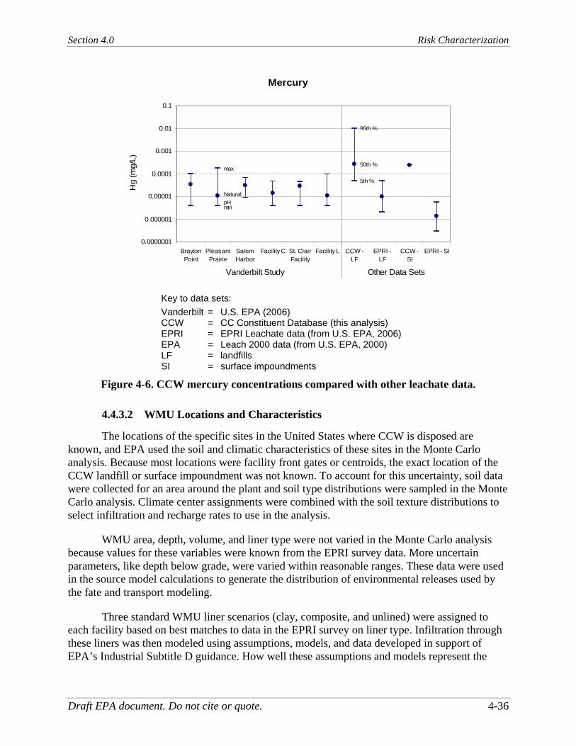
Section 4.0 Risk Characterization
Draft EPA document. Do not cite or quote. 4-36
Mercury
0.0000001
0.000001
0.00001
0.0001
0.001
0.01
0.1
BraytonPoint
PleasantPrairie
SalemHarbor
Facility C St. ClairFacility
Facility L CCW -LF
EPRI -LF
CCW -SI
EPRI - SI
Vanderbilt Study Other Data Sets
Hg
(mg/
L)
max
Natural pHmin
95th %
50th %
5th %
Key to data sets: Vanderbilt = U.S. EPA (2006) CCW = CC Constituent Database (this analysis) EPRI = EPRI Leachate data (from U.S. EPA, 2006) EPA = Leach 2000 data (from U.S. EPA, 2000) LF = landfills SI = surface impoundments
Figure 4-6. CCW mercury concentrations compared with other leachate data.
4.4.3.2 WMU Locations and Characteristics
The locations of the specific sites in the United States where CCW is disposed are known, and EPA used the soil and climatic characteristics of these sites in the Monte Carlo analysis. Because most locations were facility front gates or centroids, the exact location of the CCW landfill or surface impoundment was not known. To account for this uncertainty, soil data were collected for an area around the plant and soil type distributions were sampled in the Monte Carlo analysis. Climate center assignments were combined with the soil texture distributions to select infiltration and recharge rates to use in the analysis.
WMU area, depth, volume, and liner type were not varied in the Monte Carlo analysis because values for these variables were known from the EPRI survey data. More uncertain parameters, like depth below grade, were varied within reasonable ranges. These data were used in the source model calculations to generate the distribution of environmental releases used by the fate and transport modeling.
Three standard WMU liner scenarios (clay, composite, and unlined) were assigned to each facility based on best matches to data in the EPRI survey on liner type. Infiltration through these liners was then modeled using assumptions, models, and data developed in support of EPA’s Industrial Subtitle D guidance. How well these assumptions and models represent the

Section 4.0 Risk Characterization
Draft EPA document. Do not cite or quote. 4-37
performance of CCW WMU landfills and surface impoundments is an uncertainty in this analysis.
4.4.3.3 Fate and Transport Model Variables
The parameter values required to model contaminant fate and transport in groundwater were obtained from site-specific, regional, and national databases. Hydrogeologic environment was assigned to each site, based on geologic maps and soil conditions; where assignments were uncertain, two or three settings might be used in the Monte Carlo analysis. Because aquifer properties are highly variable and uncertain, reasonable sets of aquifer properties were selected, based on hydrogeologic environment, from a hydrogeologic database.
Receptor Location (Drinking Water Wells). The sensitivity analysis (Section 4.3) showed that distance of a receptor from the contaminant source is an important influence on media concentration, especially for contaminants that strongly sorb to soil and aquifer materials. For the groundwater-to-drinking-water pathway, receptor location was represented as the distance and position, relative to a contaminant plume, of residential drinking water wells from the WMU. Because no data were readily available on the distance of CCW disposal sites from residential wells, EPA used data from a survey of well distances from MSW landfills. Whether or not this is an accurate representation of well distance for CCW landfills and surface impoundment is one of the larger uncertainties in this analysis. EPA believes that the MSW well distance distribution used is protective for CCW landfills and surface impoundments.
Location and Characteristics of Waterbodies. One aspect of the site configuration of particular relevance to the aquatic food chain modeling is the locations and characteristics of the waterbodies. The size of the waterbodies (and the distance from the WMU) affects constituent concentrations and loadings predicted for that waterbody. The location of the waterbody was based on an empirical distribution of measurements, taken from actual CCW sites, of the distance from the edge of the WMU to the nearest stream or lake. The uncertainty posed in this analysis is the sampling of this distribution as compared to a more certain measurement of the actual distance at each CCW site. Surface water variables, including flow and water quality parameters, were collected for the stream reach being modeled, or for a larger hydrologic region where data were not available for a particular reach.
Environmental Parameters. Uncertainties related to environmental parameters (soil, aquifer, surface water, climate data) have already been mentioned. The parameters with the largest impact on results are aquifer hydraulic conductivity and gradient, which are selected from a national database of aquifer properties.
Fish Bioconcentration and Bioaccumulation Factors. For fish consumption, exposure dose is calculated using BCFs to estimate the transfer of pollutants from environmental media into fish. Uncertainty is associated with models used to estimate BCFs for aquatic biota. The aquatic BCFs were developed based on total surface water concentrations and concentrations in aquatic biota.

Section 4.0 Risk Characterization
Draft EPA document. Do not cite or quote. 4-38
4.4.3.4 Exposure and Risk Modeling Variables
Exposure parameters and benchmarks for human and ecological risk also contribute to parameter variability and uncertainty.
Human Exposure Factors. Individual physical characteristics, activities, and behavior are quite different, and thus the exposure factors that influence the exposure of an individual, including ingestion rate, body weight, and exposure duration, are quite variable. Exposure modeling relies heavily on default assumptions concerning population activity patterns, mobility, dietary habits, body weights, and other factors. The probabilistic assessment for the adult and child exposure scenario addressed the possible variability in the exposure modeling by using statistical distributions for these variables for each receptor in the assessment: adult and child resident and adult and child recreational fisher. Data on fish consumption rates are not available for children; thus the adult data were used for children in this analysis, which could overestimate risk from this pathway for children. For all exposure factors varied, a single exposure factor distribution was used for adults for both males and females. For child exposures, one age (age 1) was used to represent the age at the start of exposure, because this age group is considered to be most sensitive for most health effects.
The Exposure Factors Handbook (U.S. EPA, 1997c,d,e) provides the current state of the science concerning exposure assumptions, and it was used throughout this assessment to establish statistical distributions of values for each exposure parameter for each receptor. There are some uncertainties, however, in the data that were used. Although it is possible to study various populations to determine various exposure parameters (e.g., age-specific soil ingestion rates or intake rates for food) or to assess past exposures (epidemiological studies) or current exposures, risk assessment is about prediction. Therefore, long-term exposure monitoring in this context is infeasible.
Diet Assumptions for Ecological Receptors. National-scale assessments often assume maximum intake of contaminated prey in the diets of primary and secondary consumers (i.e., 100 percent of the diet originates from the contaminated area). Under field conditions, many receptors are opportunistic feeders with substantial variability in both the type of food items consumed as well as the geospatial patterns of feeding and foraging. The actual proportion of wildlife receptors’ diets that would be contaminated depends on a number of factors such as the species’ foraging range, quality of food source, season, intra- and interspecies competition. Consequently, the exclusive diet of contaminated food items tends to provide a very conservative estimate of potential risks.
Human Health Benchmarks. EPA routinely accounts for uncertainty in its development of RfDs and other human health benchmarks. For example, if certain toxicological data are missing from the overall toxicological database (e.g., reproductive data), EPA accounts for this by applying an uncertainty factor. In general, EPA human health benchmarks are derived using a health-protective approach.
Ecological Criteria. CSCLs were developed for constituents when sufficient data were available. In many cases, sufficient data were unavailable for a receptor/constituent combination, and therefore, the potential risk to a receptor could not be assessed. In particular, insufficient

Section 4.0 Risk Characterization
Draft EPA document. Do not cite or quote. 4-39
data were available to derive chronic effects CSCLs for amphibians. Because the risk results can only be interpreted within the context of available data, the absence of data can not be construed to mean that adverse ecological effects will not occur.
In addition to the effects of data gaps on ecological benchmarks, the ecological criteria tend to be fairly conservative because the overall approach is based on “no effects” or “lowest effects” study data. In site-specific assessments, a de minimis effects approach is often replaced with an effects level similar to natural population variability (e.g., sometimes as high as a 20 percent effects level). As a result, the CSCLs used in this analysis are likely to overestimate risks for representative species and communities assumed to live in surface waters impacted by CCW WMUs. Because the difference between a lowest observed adverse effect level (LOAEL) and a NOAEL is often about a factor of 10, an HQ exceedance of roughly 10 may not be ecologically significant. In contrast, CSCLs based on no effects data that are developed for the protection of threatened and endangered species are presumed to be protective.
4.5 Summary and Conclusions
One of the most sensitive parameters in the risk assessment is infiltration rate. Infiltration rate is greatly influenced by whether and how a WMU is lined. The 1994 to 2004 DOE/EPA survey results (U.S. DOE, 2006) do not include how many unlined facilities are still operating today, but do indicate that more facilities are lined today than were in the 1995 EPRI survey data set on which this risk assessment is based. This suggests that the risks from future CCW disposal facilities are likely to be lower than the results presented in this report. EPA will continue to work to integrate the DOE/EPA survey data into the CCW risk assessment and is seeking comments on how to address data gaps, in particular: (1) how to estimate the overall prevalence of liners in the CCW disposal facilities today, (2) how to determine the area and capacity of newer CCW landfills and surface impoundments, and (3) how the liners currently in CCW WMUs perform when compared to the industrial liner conditions assumed in this risk assessment.
Composite liners, as modeled in this risk assessment, effectively reduce risks from all pathways and constituents below the risk criteria for both landfills and surface impoundments.12 The CCW risk assessment suggests that the management of CCW in unlined landfills and unlined surface impoundments may present risks to human health and the environment. Risks from clay-lined units, as modeled, are about one-third to one-half the risks of unlined units, but are still above the risk criteria used for this analysis. These risk results are largely consistent with damage cases compiled by EPA (U.S. EPA, 2000, 2003e, 2007) and others (Lang and Schlictmann, 2004; Zillmer and Fauble, 2004; Carlson and Adriano, 1993). Key risk findings include the following:
For humans exposed via the groundwater-to-drinking-water pathway, arsenic in CCW landfills poses a 90th percentile cancer risk of 5x10⁻⁴ for unlined units and 2x10⁻⁴ for clay-lined units. The 50th percentile risks are 1x10⁻⁵ (unlined units) and 3x10⁻⁶(clay-lined
12 These results suggest that with the higher prevalence of composite liners in new CCW disposal facilities, future
national risks from onsite CCW disposal are likely to be lower than those presented in this risk assessment (which is based on 1995 CCW WMUs).

Section 4.0 Risk Characterization
Draft EPA document. Do not cite or quote. 4-40
units). Risks are higher for surface impoundments, with an arsenic cancer risk of 9x10⁻³ for unlined units and 3x10⁻³ for clay-lined units at the 90th percentile. At the 50th percentile, risks for unlined surface impoundments are 3x10⁻⁴, and clay-lined units show a risk of 9x10⁻⁵. Five additional constituents have 90th percentile noncancer risks above the criteria (HQs ranging from greater than 1 to 4) for unlined surface impoundments, including boron and cadmium, which have been cited in CCW damage cases referenced above. Boron and molybdenum show HQs of 2 and 3 for clay-lined surface impoundments. None of these noncarcinogens show HQs above 1 at the 50th percentile for any unit type.
Arrival times of the peak concentrations at a receptor well are much longer for landfills (hundreds to thousands of years) than for surface impoundments (most less than 100 years).
For humans exposed via the groundwater-to-surface-water (fish consumption) pathway, selenium (HQ = 2) and arsenic (cancer risk = 2x10⁻⁵) pose risks slightly above the risk criteria for unlined surface impoundments at the 90th percentile. For both constituents, lined 90th percentile risks and all 50th percentile risks are below the risk criteria. No constituents pose risks above the risk criteria for landfills at the 90th or 50th percentile.
Waste type has little effect on landfill risk results, but in surface impoundments, risks are up to 1 order of magnitude higher for codisposed CCW and coal refuse than for conventional CCW.
The higher risks for surface impoundments than landfills are likely due to higher waste leachate concentrations, a lower proportion of lined units, and the higher hydraulic head from the impounded liquid waste. This is consistent with damage cases reporting wet handling as a factor that can increase risks from CCW management.
For ecological receptors exposed via surface water, risks for landfills exceed the risk criteria for boron and lead at the 90th percentile, but 50th percentile risks are well below the risk criteria. For surface impoundments, 90th percentile risks for several constituents exceed the risk criteria, with boron showing the highest risks (HQ = 2,000). Only boron exceeds the risk criteria at the 50th percentile (HQ = 4). Exceedances for boron and selenium are consistent with reported ecological damage cases, which include impacts to waterbodies through the groundwater-to-surface-water pathway.
For ecological receptors exposed via sediment, 90th percentile risks for lead, arsenic, and cadmium exceeded the risk criteria for both landfills and surface impoundments because these constituents strongly sorb to sediments in the waterbody. The 50th percentile risks are generally an order of magnitude or more below the risk criteria.
Sensitivity analysis results indicate that for most of the scenarios evaluated (over 75 percent), the risk assessment model was most sensitive to parameters related to groundwater flow and transport: WMU infiltration rate, leachate concentration, and aquifer hydraulic conductivity and gradient. For strongly sorbing contaminants (such as lead and cadmium), variables related to sorption and travel time (adsorption coefficient, depth to groundwater, receptor well distance) are most important.

Section 4.0 Risk Characterization
Draft EPA document. Do not cite or quote. 4-41
There are uncertainties associated with the CCW risk assessment, but scenario uncertainty (i.e., uncertainty about the environmental setting around the plant) has been minimized by basing the risk assessment on conditions around existing U.S. coal-fired power plants around the United States. Uncertainty in environmental setting parameters has been incorporated into the risk assessment by varying these inputs within reasonable ranges when the exact value is not known. Uncertainty in human exposure factors (such as exposure duration, body weight, and intake rates) has also been addressed through the use of national distributions.
Some uncertainties not addressed explicitly in the risk assessment have been addressed through comparisons with other studies and data sources.
Appropriateness of CCW leachate data. Data on another highly sensitive parameter, leachate (porewater) constituent concentration, were available and used for CCW surface impoundments. However, available data for landfills were mainly TCLP analyses, which may not be representative of actual CCW leachate. Comparisons with recent (2006) studies of coal ash leaching processes show very good agreement for arsenic. However, although the selenium CCW data are within the range of the 2006 data, some of the higher concentrations in the 2006 data are not represented by the TCLP data. This suggests that selenium risks may be underestimated, which is consistent with selenium as a common driver of the damage cases.
Impacts of mercury rules (CAIR and CAMR). While CAIR and CAMR will reduce emissions of mercury and other metals from coal-fired power plants, mercury and other more volatile metals will be transferred from the flue gas to fly ash and other air pollution control residues, including the sludge from wet scrubbers. EPA ORD has research underway to evaluate changes to CCW characteristics and leaching of mercury and other metals from CAIR and CAMR. Data from the first report (U.S. EPA, 2006) suggest that although total mercury will increase in CCW from the use of sorbents as mercury controls, the leachability of mercury may be reduced, but this work is ongoing and should be regarded as preliminary and limited at this time. For example, wet scrubbers have yet to be addressed, and initial data from both EPA and industry studies suggest that mercury may not be as stable as found from fly ash in the first report. As these data become available, EPA will consider how best to use them to update the existing risk assessment.
Mercury and nondetect analyses. Because of a high proportion of nondetect values and a limited number of measurements, the risks from mercury in CCW could not be evaluated for either landfills or surface impoundments and for antimony and thallium in surface impoundments. The 2006 leaching study data suggest that mercury levels are fairly low in fly ash from coal combustion, but additional data and analyses would be required to estimate the risks from these levels.
Arsenic speciation. The current model does not speciate metals in the subsurface, which is of particular concern for arsenic. Damage cases and other studies suggest that arsenic readily converts from arsenic III in CCW leachate to the less mobile arsenic V in soil and groundwater. However, model runs conducted for both species suggest that the difference in risk between the two species is only about a factor of 2, which is not enough to reduce the 90th percentile cancer risks to below the risk criteria.

Section 4.0 Risk Characterization
Draft EPA document. Do not cite or quote. 4-42
Uncertainties that are more difficult to evaluate with respect to CCW risk results include the following:
Well distance. Nearest well distances were taken from a survey of MSW landfills, as data were not available from CCW sites. EPA believes that this is a protective assumption because MSW landfills generally tend to be in more populated areas, but there are little data available to test this hypothesis.
Liner conditions. Liner design and performance for CCW WMUs were based on data and assumptions EPA developed to be appropriate for nonhazardous industrial waste landfills. EPA believes that CCW landfills should have similar performance characteristics, but does not have the quantitative data to verify that.
Data gaps for ecological receptors. Insufficient data were available to develop screening levels and quantitative risk estimates for terrestrial amphibians, but EPA acknowledges that damage cases indicate risk to terrestrial amphibian and plant communities through exposure to selenium and boron.
Ecosystems and receptors at risk. Certain critical assessment endpoints were not evaluated in this analysis, including impacts on managed lands, critical habitats, and threatened and endangered species. These would be addressed through more site-specific studies on the proximity of these areas and species to CCW disposal units.
Synergistic risk. The impact of exposures of multiple contaminants to human and ecological risks was not evaluated in this analysis. EPA recognizes that a single-constituent analysis may underestimate risks associated with multiple chemical exposures.
These are potentially the more significant uncertainties associated with the CCW risk assessment. Other uncertainties are discussed in Section 4.4.

Section 5.0 References
Draft EPA document. Do not cite or quote. 5-1
5.0 References ATSDR (Agency for Toxic Substances and Disease Registry). 2002. Minimal Risk Levels
(MRLs) for Hazardous Substances. http://www.atsdr.cdc.gov/mrls.html
Barrows, M.E., S.R. Petrocelli, K.J. Macek, and J.J. Carroll. 1980. Chapter 24: Bioconcentration and elimination of selected water pollutants by bluegill sunfish (Lepomis macrochirus). In Dynamics, Exposure and Hazard Assessment of Toxic Chemicals. Edited by R. Haque. Ann Arbor, MI: Ann Arbor Science.
Bonaparte, R., J.P. Giroud, and B.A. Cross. 1989. Rates of leakage through landfill liners. Geosynthetics 1989 Conference. San Diego, CA.
Carlson, C.L., and D.C. Adriano. 1993. Environmental impacts of coal combustion residues. J. Environ. Qual. 22(227-247).
Drever, J.I. 1988. The Geochemistry of Natural Waters, 2d ed. Englewood Cliffs NJ: Prentice-Hall.
Eisler, R. 1989. Molybdenum Hazards to Fish, Wildlife, and Invertebrates: A Synoptic Review. Contaminant Hazard Reviews, Report No. 19, Biological Report 85(1.19). Laurel, MD. August.
EPRI (Electric Power Research Institute). 1997. Coal Combustion By-Products and Low-Volume Wastes Comanagement Survey. Palo Alto, CA. June.
Hopkins, W.A., S.E. DuRant, B.P. Staub, C.L. Rowe, and B.P. Jackson. 2006. Reproduction, embryonic development, and maternal transfer of contaminants in the amphibian Gastrophryne carolinensis. Environmental Health Perspectives. 114(5):661–666.
Kool, J.B., P.S. Huyakorn, E.A. Sudicky, and Z.A. Saleem. 1994. A composite modeling approach for subsurface transport of degrading contaminants from land-disposal sites. J. Contaminant Hydrology 17:69–90.
Kumada, H., S. Kimura, M. Yokote, and Y. Matida. 1972. Acute and chronic toxicity, uptake, and retention of cadmium in freshwater organisms. Bulletin of Freshwater Fisheries Research Laboratory 22(2):157–165. December 20.
Lang, D.J., and J.R. Schlictmann. 2004. Leaching of arsenic from a fly ash dump in Beverly, Massachusetts. In Proceedings of State Regulation of Coal Combustion By-Product Placement at Mine Sites. May 4–6, 2004, Harrisburg, Pennsylvania. U.S. Department of the Interior, Office of Surface Mining, Alton, IL.

Section 5.0 References
Draft EPA document. Do not cite or quote. 5-2
Lemly, A.D. 1985. Toxicology of selenium in a freshwater reservoir: Implications for environmental hazard evaluation and safety. Ecotoxicology and Environmental Safety 10:314–338.
Newell, C.J., L.P. Hopkins, and P.B. Bedient. 1989. Hydrogeologic Database for Ground Water Modeling. API Publication No. 4476. American Petroleum Institute, Washington, DC.
Newell, C,J., L.P. Hopkins, and P.B. Bedient. 1990. A hydrogeologic database for ground water modeling. Ground Water 28(5):703–714.
Schroeder, P.R., T.S. Dozier, P.A. Zappi, B.M. McEnroe, J.W. Sjostrom, and R.L. Peton. 1994a. The Hydrologic Evaluation of Landfill Performance Model (HELP): User’s Guide for Version 3. EPA/600/R-94/168a. U.S. EPA Risk Reduction Engineering Laboratory, Cincinnati, OH.
Schroeder, P.R., T.S. Dozier, P.A. Zappi, B.M. McEnroe, J.W. Sjostrom, and R.L. Peton. 1994b. The Hydrologic Evaluation of Landfill Performance (HELP) Model: Engineering Documentation for Version 3. EPA/600/R-94/168b. U.S. EPA Risk Reduction Engineering Laboratory, Cincinnati, OH.
SAB (Science Advisory Board). 2004. Review of EPA’s Multimedia, Multipathway, and Multireceptor Risk Assessment (3MRA) Modeling System. Report of the 3MRA Review Panel of the EPA Science Advisory Board. EPA-SAB-05-003, November.
Stephan, C.E., D.I. Mount, D.J. Hansen, J.H. Gentile, G.A. Chapman, and W.A. Brungs. 1985. Guidelines for Deriving Numerical National Ambient Water Quality Criteria for the Protection of Aquatic Organisms and Their Use. NTIS PB85-220749. U.S. Environmental Protection Agency, Office of Research and Development, Springfield, VA.
Stephan, C.E. 1993. Derivation of Proposed Human Health and Wildlife Bioaccumulation Factors for the Great Lakes Initiative (Draft). PB93-154672. Environmental Research Laboratory, Office of Research and Development, Duluth, MN. March.
Stumm, W., and J.J. Morgan. 1996. Aquatic Chemistry, Chemical Equilibria and Rates in Natural Waters. 3d ed. New York: John Wiley & Sons, Inc.
TetraTech. 2001. Characterization of Infiltration Rate Data to Support Groundwater Modeling Efforts (Draft). Prepared for the Office of Solid Waste, U.S. Environmental Protection Agency, Washington, DC. Contract No. 68-W6-0061. May.
U.S. DOE (Department of Energy). 2006. Coal Combustion Waste Management at Landfills and Surface Impoundments, 1994-2004. DOE/PI-0004, ANL-EVS/06-4. Office of Scientific and Technical Information, Oak Ridge, TN. August.
U.S. EPA (Environmental Protection Agency). 1988a. National Survey of Solid Waste (Municipal) Landfill Facilities (Draft). EPA/530-SW88-034. Office of Solid Waste, Washington, DC. September.
Section 5.0 References
Draft EPA document. Do not cite or quote. 5-3
U.S. EPA (Environmental Protection Agency). 1988b. Wastes from the Combusion of Coal by Electric Utility Power Plants—Report to Congress. EPA 530-SW-88-002. U.S. EPA Office of Solid Waste and Emergency Remediation. Washington, DC. February.
U.S. EPA (Environmental Protection Agency). 1988c. Design, Construction and Evaluation of Clay Liners for Waste Management Facilities. EPA-530-SW-86-007F. Office of Solid Waste and Emergency Response. Washington, DC. November.
U.S. EPA (Environmental Protection Agency). 1992. Guidelines for exposure assessment. Final guidelines. Federal Register 57 FR 22888-22893. Washington, DC. May 29.
U.S. EPA (Environmental Protection Agency). 1995. Review of EPA’s Composite Model for Leachate Migration with Transformation Products-EPACMTP. EPA-SAB-EEC-95-010. Science Advisory Board Exposure Model Subcommittee of the Environmental Engineering Committee. Washington, DC.
U.S. EPA (Environmental Protection Agency). 1996. EPA’s Composite Model for Leachate Migration with Transformation Products. EPACMTP: Background Document. Office of Solid Waste, Washington, DC.
U.S. EPA (Environmental Protection Agency). 1997a. EPA’s Composite Model for Leachate Migration with Transformation Products. EPACMTP: User’s Guide. Office of Solid Waste, Washington, DC.
U.S. EPA (Environmental Protection Agency). 1997b. Mercury Study Report to Congress. Volume III, Fate and Transport of Mercury in the Environment. EPA 452/R-97/005. Office of Air Quality Planning and Standards and Office of Research and Development, Washington, DC.
U.S. EPA (Environmental Protection Agency). 1997c. Exposure Factors Handbook, Volume I, General Factors. EPA/600/P-95/002Fa. Office of Research and Development, Washington, DC. August.
U.S. EPA (Environmental Protection Agency). 1997d. Exposure Factors Handbook, Volume II, Food Ingestion Factors. EPA/600/P-95/002Fa. Office of Research and Development, Washington, DC. August.
U.S. EPA (Environmental Protection Agency). 1997e. Exposure Factors Handbook, Volume III, Activity Factors. EPA/600/P-95/002Fa. Office of Research and Development, Washington, DC. August.
U.S. EPA (Environmental Protection Agency). 1997f. Health Effects Assessment Summary Tables (HEAST). EPA-540-R-97-036. FY 1997 Update. Office of Solid Waste and Emergency Response, Washington, DC.
U.S. EPA (Environmental Protection Agency). 1998a. Non-Groundwater Pathways, Human Health and Ecological Risk Analysis for Fossil Fuel Combustion Phase 2 (FFC2): Draft Final Report. Office of Solid Waste, Washington, DC. June.

Section 5.0 References
Draft EPA document. Do not cite or quote. 5-4
U.S. EPA (Environmental Protection Agency). 1998b. Technical Background Document for the Supplemental Report to Congress on Remaining Fossil Fuel Combustion Wastes: Ground-Water Pathway Human Health Risk Assessment. Revised Draft Final. Office of Solid Waste, Washington, DC. June.
U.S. EPA (Environmental Protection Agency). 1998c. Methodology for Assessing Health Risks Associated with Multiple Pathways of Exposure to Combustor Emissions. Update to Methodology for Assessing Health Risks Associated with Indirect Exposure to Combustor Emissions. EPA-600/R-98/137. National Center for Environmental Assessment, Cincinnati, OH.
U.S. EPA (Environmental Protection Agency). 1998d. Human Health Risk Assessment Protocol for Hazardous Waste Combustion Facilities, Volume One. EPA-530-D-98-001A. Office of Solid Waste and Emergency Response, Washington, DC.
U.S. EPA (Environmental Protection Agency). 1999a. Report to Congress: Wastes from the Combustion of Fossil Fuels. EPA 530-R-99-010. Office of Solid Waste, Washington, DC. March.
U.S. EPA (Environmental Protection Agency). 1999b. Partition Coefficients for Metals in Surface Water, Soil, and Waste. Office of Solid Waste, Washington, DC. http://www.epa.gov/ epaoswer/hazwaste/id/hwirwste/pdf/risk/reports/s0524.pdf.
U.S. EPA (Environmental Protection Agency). 1999c. Peer Review of EPA’s Hazardous Waste Identification Rule Risk Assessment Model - The Vadose Zone and Saturated Zone Modules Extracted From EPACMTP for HWIR99. Prepared by Eastern Research Group under EPA Contract No. 68-W-99-001, Work Assignment No. 17, for Office of Solid Waste. Washington, DC. Available at http://www.epa.gov/epaoswer/hazwaste/id/ hwirwste/peer03/vadoze/vz-aquif.pdf#search=%22EPACMTP%20peer%20review%22.
U.S. EPA (Environmental Protection Agency). 1999d. Peer Review of EPA’s Hazardous Waste Identification Rule Risk Assessment Model - MINTEQA2/PRODEFA2 Version 4.0. Prepared by Eastern Research Group under EPA Contract No. 68-W-99-001, Work Assignment No. 17, for Office of Solid Waste. Washington, DC. Available at http://www.epa.gov/epaoswer/hazwaste/id/hwirwste/peer03/minteqa2/minteqa2.pdf.
U.S. EPA (Environmental Protection Agency). 2000. Review of Causative Factors for Coal Combustion Waste Damage Cases. Prepared by SAIC for U.S. EPA Office of Solid Waste under EPA contract 68-W-99-001, WA No. 121. Washington, DC. November 29.
U.S. EPA (Environmental Protection Agency). 2001a. Revisions in Input Data and Modeling Procedures for Using MINTEQA2 in Estimating Metal Partition Coefficients. Prepared by Allison Geoscience Consultants, Inc., for the Office of Solid Waste, Washington, DC.
U.S. EPA (Environmental Protection Agency). 2001b. WATER9, Air Emission Models for Waste and Wastewater. Technology Transfer Network Clearinghouse for Inventories & Emission Factors. http://www.epa.gov/ttn/chief/software/water

Section 5.0 References
Draft EPA document. Do not cite or quote. 5-5
U.S. EPA (Environmental Protection Agency). 2001c. Risk Assessment Paper for Derivation of a Provisional RfD for Cobalt and Compounds (CASRN 7440-48-4). 00-122/3-16-01. National Center for Environmental Assessment, Superfund Technical Support Center, Cincinnati, OH.
U.S. EPA (Environmental Protection Agency). 2001d. Risk Assessment Paper for Derivation of a Provisional Carcinogenicity Assessment for Cobalt and Compounds (CASRN 7740-48-4). 00-122/3-16-01. National Center for Environmental Assessment. Superfund
U.S. EPA (Environmental Protection Agency). 2002a. Constituent Screening for Coal Combustion Wastes. Draft Report prepared by Research Triangle Institute for Office of Solid Waste, Washington, DC. September.
U.S. EPA (Environmental Protection Agency). 2002b. Industrial Waste Management Evaluation Model (IWEM) Technical Background Document. EPA530-R-02-012. Office of Solid Waste, Washington, DC. August.
U.S. EPA (Environmental Protection Agency). 2002c. Integrated Risk Information System (IRIS). National Center for Environmental Assessment, Office of Research and Development, Washington, DC. http://www.epa.gov/iris/.
U.S. EPA (Environmental Protection Agency). 2002d. Current Drinking Water Standards. National Primary and Secondary Drinking Water Regulations. Office of Ground Water and Drinking Water, Washington, DC. http://www.epa.gov/safewater/mcl.html.
U.S. EPA (Environmental Protection Agency). 2003a. EPA’s Composite Model for Leachate Migration with Transformation Products (EPACMTP): Parameters/Data Background Document. Office of Solid Waste, Washington, DC. April. http://www.epa.gov/epaoswer/non-hw/industd/tools/cmtp/epacmtp.htm#data.
U.S. EPA (Environmental Protection Agency). 2003b. Risk Assessment Technical Background Document for the Dye and Pigment Industry Hazardous Waste Listing Determination. OMB Review Draft. Office of Solid Waste, Washington, DC.
U.S. EPA (Environmental Protection Agency). 2003c. EPACMTP Technical Background Document. Office of Solid Waste, Washington, DC.
U.S. EPA (Environmental Protection Agency). 2003d. Addendum to the EPACMTP Technical Background Document. Office of Solid Waste, Washington, DC.
U.S. EPA (Environmental Protection Agency). 2003e. Final Revised Report on Resolution of 18 Previously Indeterminate Candidate Damage Cases. Prepared by SAIC for U.S. EPA Office of Solid Waste under EPA contract 68-W-02-036, WA No. 1-12. Washington, DC. March 5.
U.S. EPA (Environmental Protection Agency). 2003f. Peer Review Of Changes To EPA's MINTEQA2 Model. Prepared by Industrial Economics for the Office of Solid Waste, Washington, DC.

Section 5.0 References
Draft EPA document. Do not cite or quote. 5-6
U.S. EPA (Environmental Protection Agency). 2005. Sensitivity Analysis for the Coal Combustion Waste Risk Assessment. Technical Report prepared by RTI International for U.S. EPA Office of Solid Waste under EPA contract 68-W-03-042, WA No. 1-16. Washington, DC. March 5.
U.S. EPA (Environmental Protection Agency). 2006. Characterization of Mercury-Enriched Coal Combustion Residues from Electric Utilities Using Enhanced Sorbents for Mercury Control. EPA 600/R-06/008. Office of Research and Development. Research Triangle Park, NC. January.
U.S. EPA (Environmental Protection Agency). 2007. Coal Combustion Waste Damage Case Assessments. Available from the docket to the Notice of Data Availability on the Disposal of Coal Combustion Wastes in Landfills and Surface Impoundments, Docket # EPA-HQ-RCRA-2006-0796. June 19.
Zilmer, M., and P. Fauble. 2004. Groundwater impacts from coal combustion ash disposal sites in Wisconsin. In: Proceedings of State Regulation of Coal Combustion By-Product Placement at Mine Sites. May 4–6, 2004, Harrisburg, Pennsylvania. U.S. Department of Interior, Office of Surface Mining, Alton, IL.

Appendix A Constituent Data
A-1
Appendix A. Constituent Data
The coal combustion waste (CCW) risk assessment addresses metals and inorganic constituents identified by EPA as potential constituents of concern in CCW (Table A-1). U.S. Environmental Protection Agency (EPA) derived waste concentrations for these constituents from its CCW constituent database, which includes analyte concentration data in three tables representing different types of waste samples: landfill leachate analyses (in mg/L), surface impoundment and landfill porewater analyses (in mg/L), and analyses of whole waste samples (in mg/kg). Each database table specifies, for most samples, the type of waste sampled and the type of coal burned at the facility.
Table A-1. Constituents Addressed in the Screening Analysis
Constituent CAS ID Constituent CAS ID Metals Inorganic Anions Aluminum 7429-90-5 Chloride 16887-00-6 Antimony 7440-36-0 Cyanide 57-12-5 Arsenic 7440-38-2 Fluoride 16984-48-8 Barium 7440-39-3 Total Nitrate Nitrogen 14797-55-8 Beryllium 7440-41-7 Phosphate 14265-44-2 Boron 7440-42-8 Silicon 7631-86-9 Cadmium 7440-43-9 Sulfate 14808-79-8 Chromium 7440-47-3 Sulfide 18496-25-8 Cobalt 7440-48-4 Inorganic Cations Copper 7440-50-8 Ammonia 7664-41-7 Iron 7439-89-6 Calcium 7440-70-2 Lead 7439-92-1 pH 12408-02-5 Magnesium 7439-95-4 Potassium 7440-09-7 Manganese 7439-96-5 Sodium 7440-23-5 Mercury 7439-97-6 Nonmetallic Elements Molybdenum 7439-98-7 Inorganic Carbon 7440-44-0 Nickel 7440-02-0 Total Elemental Sulfur 7704-34-9 Selenium 7782-49-2 Measurements Silver 7440-22-4 Total Dissolved Solids none Strontium 7440-24-6 Total Organic Carbon none Thallium 7440-28-0 Dissolved Organic Carbon none Vanadium 7440-62-2 Zinc 7440-66-6

Appendix A Constituent Data
A-2
A.1 Data Sources
EPA prepared the CCW constituent database in 2002 and 2003. The 2003 CCW constituent database includes all of the waste characterization data used by EPA in its risk assessments in support of the March 1999 Report to Congress: Wastes from the Combustion of Fossil Fuels (the RTC) (U.S. EPA, 1999). In addition to the data set from the March 1999 RTC, EPA supplemented the database with the following data:
Data submitted with public comments to EPA on the 1999 RTC
Data submitted with public comments to EPA concerning the May 22, 2000, Final Regulatory Determination
Data collected by and provided to EPA since the end of the public comment period on the Final Regulatory Determination
Data identified from literature searches.
The primary sources of these additional data include the electric power industry, state and federal regulatory agencies, and scientific literature. Attachment A-1 is a complete list of the sources of data contained in the 2003 CCW constituent database.
The additional data represent a significant expansion in the quantity of characterization data available to EPA for analysis. For example, the data set used for the risk assessments supporting the RTC covered approximately 50 CCW generation and/or disposal sites. With the addition of the supplemental data, the 2003 CCW constituent database now covers more than 160 sites. The 1999 data set included approximately 10,000 individual samples of CCW. The 2003 CCW constituent database now includes more than 35,000 individual samples.
The additional data also represent an expansion in the scope of characterization data available to EPA for analysis. The 1999 data were obtained exclusively from the electric power industry. As shown in Attachment A-1, the 2003 data set includes data from other sources, such as scientific literature and state and federal regulatory agencies. The 1999 data set included analyses of whole waste samples, surface impoundment and landfill porewater analyses, and analyses of extracts obtained using the Toxicity Characteristic Leaching Procedure (TCLP), the Synthetic Precipitation Leaching Procedure (SPLP), and Extraction Procedure (EP) Toxicity leaching methods. The 2003 data set adds analyses of actual landfill leachate (e.g., obtained from leachate collection systems), analyses of extracts obtained using other leaching methods (including higher retention time leaching methods), and porewater analyses.
The 2003 CCW constituent database represents CCW characteristics across a broad cross section of the generating universe. Not only does the database include data from a large number of sites, but these sites are distributed throughout the United States, as shown in Table A-2. The database includes data for all major types of CCW (i.e., fly ash, bottom ash, flue gas desulfurization [FGD] sludge, fluidized bed combustion [FBC] fly ash, and FBC bed ash), from mixtures of CCW types that are commonly created during disposal operations (e.g., combined fly ash and bottom ash), and from CCW mixed with coal refuse (a common disposal practice). Section A.2 discusses waste types in more detail.

Appendix A Constituent Data
A-3
Table A-2. States Included in the CCW Constituent Database
Alaska Illinois Maryland Arkansas Indiana Michigan California Kentucky Ohio Colorado Missouri Oklahoma Connecticut North Carolina Pennsylvania Florida North Dakota Tennessee Georgia Nebraska Texas Hawaii New Mexico Wisconsin Iowa Louisiana West Virginia
The database also includes data for CCW generated from combustion of all major coal ranks: bituminous, sub-bituminous, lignite, and anthracite. Although the database does include coal type designations for most of the entries, in many cases the type is not specified. In addition, many coal plants mix coal from different sources (e.g., eastern and western coals), depending on prices and the need to reduce sulfur levels. As a result, correlations of risk results with coal types may be difficult and may not produce significant results.
A.2 Data Preparation
Table A-3 lists the waste types evaluated in the CCW risk assessment, along with the number of sites representing each waste type in the CCW constituent database. Key steps in preparing these data for screening include (1) selection and grouping of waste types to be addressed, (2) selection of the analyte data to be used, and (3) processing of these data to develop the analyte concentrations for the screening analysis.
Table A-3. Waste Streams in CCW Constituent Database
Number of Sites by Waste Typea
Waste Type Waste Streams
Landfill Leachate
Surface Impoundment
Porewater Total Waste Conventional Combustion Waste 97 13 62 Ash (not otherwise specified) 43 0 30 Fly ash 61 2 33 Bottom ash & slag 24 3 23 Combined fly & bottom ash 7 4 4 FGD sludge 4 6 5 Codisposed Ash & Coal Refuse 9 5 1 Fluidized Bed Combustion Waste 58 0 54 Ash (not otherwise specified) 18 0 10 Fly ash 33 0 32 Bottom and bed ash 26 0 25 Combined fly & bottom ash 20 0 22 a Site counts by waste type from leachate, porewater, and whole waste data tables in the 2003 CCW
constituent database.
Appendix A Constituent Data
A-4
A.2.1 Selection and Grouping of Waste Types of Concern
The CCW constituent database contains a variety of waste types. Some selection and grouping of these types was appropriate so that the risk assessment could evaluate risks consistently for groups of wastes that are expected to behave similarly when disposed in landfills and surface impoundments.
Combustion ash types in the CCW constituent database include fly ash, bottom ash, bed ash, slag, combined fly and bottom ash, and coal ash not otherwise specified. Based on a statistical analysis that showed no significant difference in leachate and porewater chemistry, the analysis combines data for these ash types for landfills and surface impoundments. FGD sludge is also combined with these conventional combustion ash types based on insignificant differences in porewater chemistry and the fact that FGD sludge is usually codisposed with varying amounts of fly ash and bottom ash.
CCW porewater constituent data did show that FBC wastes and codisposed ash and coal refuse (coal waste from coal crushers and other coal preparation and handling operations1) differ significantly from coal combustion ash in their composition and leachate chemistry, so these wastes were addressed separately in the risk analysis. FBC waste chemistry is impacted by the limestone injected with coal in FBC units for sulfur capture and tends to be very alkaline with high levels of calcium and sulfate. Coal refuse is high in pyrite, which generates sulfuric acid when disposed. As a result, combustion wastes exhibit a lower pH when codisposed with coal refuse.
A.2.2 Selection of Appropriate Analyte Data
CCW analyte concentration data represent leachate from landfills and surface impoundments and whole waste in landfills, as follows:
Whole waste analyte concentrations (in mg/kg) represent landfill waste.
Analyte concentrations (in mg/L) in porewater sampled from surface impoundment sediments represent surface impoundment leachate.
Analyte concentrations for extracts from leaching methods, analyses of actual landfill leachate, and landfill porewater analyses represent landfill leachate. Because the CCW constituent database includes analyte concentrations from several leaching methods, a decision hierarchy was used to select leachate analyses to use in the risk assessment (Table A-4).
As shown in Table A-4, the methods thought to best represent long-term waste monofill porewater composition (i.e., methods with long equilibration times and low liquid-to-solid ratios) represent only a few sites, with most sites having TCLP and/or SPLP measurements. To best represent CCW landfill waste concentration at a wide variety of sites, the hierarchy rank shown in Table A-4 was used to select the best method for a particular site. For sites where two or more 1 Coal refuse is the waste coal produced from coal handling, crushing, and sizing operations. In the CCW constituent
database, codisposed coal refuse includes “combined ash and coal gob”, “combined ash and coal refuse”, and “combined bottom ash and pyrites”.

Appendix A Constituent Data
A-5
methods are available in the same rank (which often occurs for SPLP and TCLP analyses), the screening analysis uses the method with the highest analyte concentrations. This ensures that the data used in the risk assessment are the best that are available and represent a broad variety of waste disposal conditions.
Table A-4. Comparison/Hierarchy of Leaching Methods for Landfills Represented in CCW Constituent Database
Method (Rank) Description Advantages Disadvantages Landfill leachate (1) Direct samples of
landfill leachate Most representative of leachate chemistry
Low number of sites represented
Landfill porewater (1) Direct porewater samples from landfill
Most representative of leachate chemistry
Low number of sites represented
High retention time and low liquid-to-solid ratio (L:S) methods (2)
Waste extractions with long equilibration times (days to weeks) and low L:S
Better representation of landfill equilibration times and L:S
Low number of sites represented
Low L:S methods (3) Waste extractions with low L:S
Better representation of landfill L:S
Low number of sites represented; equilibrium times relatively short
High retention time methods (3)
Waste extractions with long equilibration times (days to weeks)
Better representation of landfill equilibration times
Low number of sites represented; L:S relatively high
TCLP (4) Toxicity Characteristic Leaching Procedure waste extractions
Most representative in terms of number of sites, waste types covered
High L:S (20:1) can dilute leachate concentrations; short equilibration time (18 hours) may not allow equilibrium to develop; Na-acetate buffer can overestimate leaching for some constituents (e.g., Pb)
SPLP (4) Synthetic Precipitation Leaching Procedure and other dilute water waste extractions
More representative in terms of number of sites, waste types covered; extract similar to precipitation
High L:S (20:1) can dilute leachate concentrations; short equilibration time (18 hours) may not allow equilibrium to develop
A.2.3 Development of Waste Constituent Concentrations
To allow risk assessment results to be organized by waste constituent and waste type, CCW data were processed to produce a single concentration per waste stream (surface impoundment porewater, landfill leachate, and landfill whole waste), analyte, and site for use in the risk assessment. Data processing to prepare these analyte concentrations for the CCW risk assessment involved two steps:
1. Calculation of average constituent concentrations by site for landfill leachate, surface impoundment porewater, and total ash concentrations. Site averaging avoids potential bias toward sites with many analyses per analyte. During site averaging, any separate waste disposal scenarios occurring at a site (e.g., non-FBC and FBC ash) were treated as separate “sites” and were averaged independently. This approach is consistent with that used in the 1998 CCW risk analysis. As in 1998, nondetects were averaged at one-half the reported detection limit.

Appendix A Constituent Data
A-6
2. Selection of waste concentrations from site-averaged values. For the Monte Carlo analysis, the analysis randomly selected, by waste type/waste management unit (WMU) scenario, site-averaged leachate concentrations. For landfills, a corresponding total waste analysis was pulled from the database or calculated from a constituent-specific relationship between landfill leachate and total waste analyses.
A.3 Constituent Screening and Selection
The CCW risk assessment employed two steps to narrow the list of CCW constituents for the full-scale Monte Carlo risk assessment. Two steps were conducted to focus the full-scale analysis on the CCW constituents of most concern:
1. Hazard Identification, which involved collection of existing human health and ecological benchmarks for the constituents of concern. Only chemicals with benchmarks moved on to risk screening.
2. Constituent Screening, which compared health-based concentration benchmarks against very conservative estimates of exposure concentrations (e.g., whole waste concentrations, leaching concentrations) to quickly and simply “screen out” constituents and exposure pathways of no significant concern.
During the hazard identification step of the CCW risk assessment, constituents of potential concern were first identified by searching, from EPA and other reputable sources, for human health and ecological benchmarks for each chemical in the CCW constituent database. Table A-5 shows the result of that search; of the 41 chemicals in the database, 26 chemicals were found to have benchmarks.
Table A-5. Toxicity Assessment of CCW Constituents Constituent CAS ID HHB EcoB Constituent CAS ID HHB EcoB Metals Inorganic Anions Aluminum 7429-90-5 U U Chloride 16887-00-6 Antimony 7440-36-0 U U Cyanide 57-12-5 U Arsenic 7440-38-2 Ua U Fluoride 16984-48-8 U Barium 7440-39-3 U U Nitrate 14797-55-8 U Beryllium 7440-41-7 Ua U Nitrite 14797-65-0 U Boron 7440-42-8 U U Phosphate 14265-44-2 Cadmium 7440-43-9 Ua U Silicon 7631-86-9 Chromium 7440-47-3 Ua U Sulfate 14808-79-8 Cobalt 7440-48-4 Ua U Sulfide 18496-25-8 Copper 7440-50-8 Ub U Inorganic Cations Iron 7439-89-6 Ammonia 7664-41-7 U Lead 7439-92-1 Ub U Calcium 7440-70-2 Magnesium 7439-95-4 pH 12408-02-5 Manganese 7439-96-5 U Potassium 7440-09-7 Mercury 7439-97-6 U U Sodium 7440-23-5 Molybdenum 7439-98-7 U U Nonmetallic Elements Nickel 7440-02-0 U U Carbon 7440-44-0 Selenium 7782-49-2 U U Sulfur 7704-34-9 Silver 7440-22-4 U U Measurements Strontium 7440-24-6 U Total Dissolved Solids none
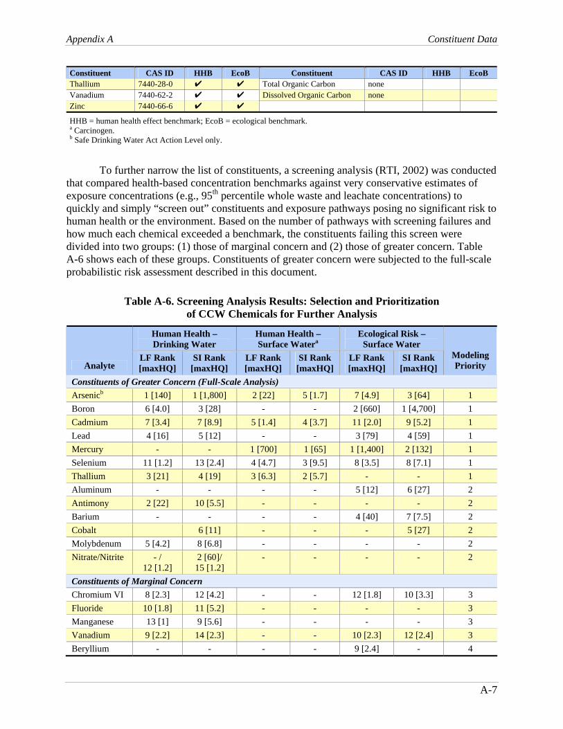
Appendix A Constituent Data
A-7
Constituent CAS ID HHB EcoB Constituent CAS ID HHB EcoB Thallium 7440-28-0 U U Total Organic Carbon none Vanadium 7440-62-2 U U Dissolved Organic Carbon none Zinc 7440-66-6 U U
HHB = human health effect benchmark; EcoB = ecological benchmark. a Carcinogen. b Safe Drinking Water Act Action Level only.
To further narrow the list of constituents, a screening analysis (RTI, 2002) was conducted that compared health-based concentration benchmarks against very conservative estimates of exposure concentrations (e.g., 95th percentile whole waste and leachate concentrations) to quickly and simply “screen out” constituents and exposure pathways posing no significant risk to human health or the environment. Based on the number of pathways with screening failures and how much each chemical exceeded a benchmark, the constituents failing this screen were divided into two groups: (1) those of marginal concern and (2) those of greater concern. Table A-6 shows each of these groups. Constituents of greater concern were subjected to the full-scale probabilistic risk assessment described in this document.
Table A-6. Screening Analysis Results: Selection and Prioritization of CCW Chemicals for Further Analysis
Human Health – Drinking Water
Human Health –Surface Watera
Ecological Risk –Surface Water
Analyte LF Rank [maxHQ]
SI Rank [maxHQ]
LF Rank [maxHQ]
SI Rank [maxHQ]
LF Rank [maxHQ]
SI Rank [maxHQ]
Modeling Priority
Constituents of Greater Concern (Full-Scale Analysis) Arsenicb 1 [140] 1 [1,800] 2 [22] 5 [1.7] 7 [4.9] 3 [64] 1 Boron 6 [4.0] 3 [28] - - 2 [660] 1 [4,700] 1 Cadmium 7 [3.4] 7 [8.9] 5 [1.4] 4 [3.7] 11 [2.0] 9 [5.2] 1 Lead 4 [16] 5 [12] - - 3 [79] 4 [59] 1 Mercury - - 1 [700] 1 [65] 1 [1,400] 2 [132] 1 Selenium 11 [1.2] 13 [2.4] 4 [4.7] 3 [9.5] 8 [3.5] 8 [7.1] 1 Thallium 3 [21] 4 [19] 3 [6.3] 2 [5.7] - - 1 Aluminum - - - - 5 [12] 6 [27] 2 Antimony 2 [22] 10 [5.5] - - - - 2 Barium - - - - 4 [40] 7 [7.5] 2 Cobalt 6 [11] - - - 5 [27] 2 Molybdenum 5 [4.2] 8 [6.8] - - - - 2 Nitrate/Nitrite - /
12 [1.2] 2 [60]/ 15 [1.2]
- - - - 2
Constituents of Marginal Concern Chromium VI 8 [2.3] 12 [4.2] - - 12 [1.8] 10 [3.3] 3 Fluoride 10 [1.8] 11 [5.2] - - - - 3 Manganese 13 [1] 9 [5.6] - - - - 3 Vanadium 9 [2.2] 14 [2.3] - - 10 [2.3] 12 [2.4] 3 Beryllium - - - - 9 [2.4] - 4

Appendix A Constituent Data
A-8
Human Health – Drinking Water
Human Health –Surface Watera
Ecological Risk –Surface Water
Analyte LF Rank [maxHQ]
SI Rank [maxHQ]
LF Rank [maxHQ]
SI Rank [maxHQ]
LF Rank [maxHQ]
SI Rank [maxHQ]
Modeling Priority
Constituents of Greater Concern (Full-Scale Analysis) Copper - - - - 14 [1.6] 11 [3.1] 4 Nickel - 16 [1.3] - - - 13 [1.4] 4 Silver - - - - 6 [11] 14 [1.4] 4 Zinc - - - - 13 [1.6] - 4 LF = landfill; maxHQ = maximum hazard quotient; SI = surface impoundment. a Fish consumption pathway. b Arsenic values for human health are [excess cancer risk / target risk (1E-05)].
A.4 Results
Attachment A-2 provides the site-averaged constituent data used in the full-scale CCW risk assessment by waste type/WMU scenario.
A.5 References
RTI (RTI International). 2002. Constituent Screening for Coal Combustion Wastes. Draft Report prepared for U.S. Environmental Protection Agency, Office of Solid Waste, Washington, DC. September.
U.S. EPA (Environmental Protection Agency). 1999. Report to Congress: Wastes from the Combustion of Fossil Fuels. EPA 530-5-99-010. Office of Solid Waste and Emergency Response, Washington, DC. March.

Appendix A Attachment A-1: Sources of Data
A-1-1
Attachment A-1: Sources of Data General Alaska Department of Environmental Conservation. 2000. Comments on Regulatory
Determination on Wastes from the Combustion of Fossil Fuels, Docket No. F-2000-FF2F-FFFFF and attachments.
Anthracite Region Independent Power Producers Association (ARIPPA). 2000. Occurrence and Fate of Selected Trace Elements in Circulating Fluidized Bed Combustion Byproducts, Volume II of II, Prepared by Earthtech Inc., Johnstown, PA, for ARIPPA.
Bhattacharja, S., J.L. Evanko, J.J. Gajda, and R.H. Carty. 2001. Ceramic tiles using Illinois fly ash. In Proceedings of the American Coal Ash Association 14th International Symposium on Management & Use of Coal Combustion Products (CCPs), January 22–26, 2001, San Antonio, TX. Palo Alto, CA: Electric Power Research Institute, EPRI 1001183, Volume 1: Management and Use of Coal Combustion Products (CCPs). Available: http://www.acaa-usa.org/store-books.htm
Bland, A.E., T.H. Brown, and D.O. Steen. 2001. Flowable fill materials made from lignite fired fluidized bed combustion ash. In Proceedings of the American Coal Ash Association 14th International Symposium on Management & Use of Coal Combustion Products (CCPs), January 22–26, 2001, San Antonio, TX. Palo Alto, CA: Electric Power Research Institute, EPRI 1001183, Volume 1: Management and Use of Coal Combustion Products (CCPs). Available: http://www.acaa-usa.org/store-books.htm
Butler, R.D., D.F. Pflughoeft-Hassett, B.A. Dockter, and H.J. Foster. 1995. Stabilization of Underground Mine Voids by Filling with Coal Conversion Residuals. Energy & Environmental Research Center, University of North Dakota, Grand Forks, ND. 43 pp.
Dairyland Power Cooperative. 1991. Letter to Wisconsin Department of Natural Resources. May 22, 1991.
Electric Power Research Institute (EPRI). 1983. Pilot Study of Time Variability of Elemental Ash Concentrations in Power-Plant Ash. EPRI-EA-2959, EPRI, Palo Alto, CA.
Electric Power Research Institute (EPRI). 1995. Laboratory Characterization of Atmospheric Fluidized-Bed Combustion By-Products, Final Report. EPRI-TR-105527, EPRI, Palo Alto, CA.
Electric Power Research Institute (EPRI). 1995. Land Application of Coal Combustion By-Products: Use in Agriculture and Land Reclamation, Final Report. EPRI-TR-103298, EPRI, Palo Alto, CA.
Electric Power Research Institute (EPRI). 1996. Fluid Placement of Fixated Scrubber Sludge in Abandoned Deep Mines to Abate Surface Subsidence and Reduce Acid Mine Drainage. EPRI-TR-107053, EPRI, Palo Alto, CA.

Appendix A Attachment A-1: Sources of Data
A-1-2
Electric Power Research Institute (EPRI). 1996. Mixtures of a Coal Combustion By-Product and Composted Yard Wastes for Use as Soil Substitutes and Amendments, Final Report. EPRI-TR-106682, EPRI, Palo Alto, CA.
Electric Power Research Institute (EPRI). 1998. Identification of Arsenic Species in Coal Ash Particles. EPRI-TR-109002, EPRI, Palo Alto, CA.
Electric Power Research Institute (EPRI). 1999. Investigation of Ammonia Adsorption on Fly Ash and Potential Impacts of Ammoniated Ash. EPRI-TR-113777, EPRI, Palo Alto, CA.
Electric Power Research Institute (EPRI). 1999. Utilization of Coal Combustion By-Products in Agriculture and Land Reclamation, Final Report. EPRI-TR-112746, EPRI, Palo Alto, CA.
Electric Power Research Institute (EPRI). 2001. Environmental Evaluation for Use of Ash in Soil Stabilization Applications. WO9227-01, EPRI, Palo Alto, CA.
Electric Power Research Institute (EPRI). n.d. Guidance for Comanagement of Mill Rejects at Coal-Fired Power Plants, Pre-Publication. EPRI-TR-108994, EPRI, Palo Alto, CA.
Finkelman, R.B., C.A. Palmer, and C.F. Eble. 1998. Characterization of hazardous trace elements in solid waste products from a coal burning power plant in Kentucky. In Characterization of Coal and Coal Combustion Products from a Coal Burning Power Plant – Preliminary Report and Results of Analysis. Edited by G.N. Breit and R.B. Finkelman. U.S. Geological Survey, Open File Report 98-342, 101 pp.
Freeman United Coal Mining Company. 1991–2001. Quarterly Ash Analyses.
Haefner, R.J. n.d. Water Quality at an Abandoned Mine Site Treated with Coal Combustion By-Products. U.S. Geological Survey, Water Resources Division, Columbus, OH. Available: http://www.mcrcc.osmre.gov/PDF/Forums/CCB2/4d.pdf
Hassett, D.J., D.F. Pflughoeft-Hassett, D.L. Laudal, and J.H. Pavlish. 1999. Mercury release from coal combustion by-products to the environment. In Mercury in the Environment, Proceedings of a Specialty Conference, Minneapolis, MN, September 15–17, Air & Waste Management Association, pp. 85–93.
Hower, J.C., J.D. Robertson, and J.M. Roberts. 2001. Coal combustion by products from the co-combustion of coal, tire-derived fuel, and petroleum coke at a western Kentucky cyclone-fired unit. In Proceedings of the American Coal Ash Association 14th International Symposium on Management & Use of Coal Combustion Products (CCPs), January 22–26, 2001, San Antonio, TX. Palo Alto, CA: Electric Power Research Institute, EPRI 1001183, Volume 1: Management and Use of Coal Combustion Products (CCPs). Available: http://www.acaa-usa.org/store-books.htm
Hower, J.C., J.D. Robertson, U.M. Graham, G.A. Thomas, A.S. Wong, and W.H. Schram. 1993. Characterization of Kentucky coal-combustion by-products: Compositional variations based on sulfur content of feed coal. Journal of Coal Quality 12:150–155.
Hower, J.C., A.S. Trimble, C.F. Eble, C.A. Palmer, and A. Kolker. 1997. Characterization of fly ash from low-sulfur and high-sulfur coal sources: Partitioning of carbon and trace elements with particle size.

Appendix A Attachment A-1: Sources of Data
A-1-3
Indiana Department of Natural Resources. 1999. Response to the U.S. Environmental Protection Agency’s March 1999 Report to Congress: Wastes from the Combustion of Fossil Fuels, Volume 2 of 3.
Kim, A.G., and G. Kazonich. 2001. Release of trace elements from CCB: Maximum extractable fraction. 2001. In Proceedings of the American Coal Ash Association 14th International Symposium on Management & Use of Coal Combustion Products (CCPs), January 22–26, 2001, San Antonio, TX. Palo Alto, CA: Electric Power Research Institute, EPRI 1001183, Volume 1: Management and Use of Coal Combustion Products (CCPs). Available: http://www.acaa-usa.org/store-books.htm
Kost, D.A., J.P. Vimmerstedt, and R.C. Stehouwer. 1997. Reclamation of Acid, Toxic Coal Spoils Using Wet Flue Gas Desulfurization By-Product, Fly Ash and Sewage Sludge.
Longley, R.D. Jr. 1997. Examination of Fly Ash Grouts to Be Used in Acid Mine Drainage Remediation.
Loop, C.M. 2000. The Impact of Ash Placement in a Surface Mine Pool on the Chemistry of the Silverbrook Basin. M.S. Thesis, University Park, PA: The Pennsylvania State University.
Mafi, S., M.T. M.T. Damian, and R. Baker. n.d. Injection of FGD grout to abate acid mine drainage in underground coal mines.
Naik, T.R., R.N. Kraus, R.F. Sturzl, and B.W. Ramme. 1998. Design and testing controlled low-strength materials (CLSM) using clean coal ash. In The Design and Application of Controlled Low-Strength Materials (Flowable Fill), Edited by A.K. Howard and J.L. Hitch, ASTM STP 1331.
Pennsylvania Department of Environmental Protection (PADEP). 1999. Pennsylvania Department of Environmental Quality Comments on EPA Report to Congress, Volume 2: Coal Ash Used as Minefill – Placement Not in Contact with Groundwater. Available: Roderick A. Fletcher, Director, Bureau of Mining and Reclamation, PADEP, Rachel Carson State Office Building, P.O. Box 8461, Harrisburg, PA 17105-8461.
Pennsylvania Department of Environmental Protection (PADEP). 1999. Pennsylvania Department of Environmental Quality Comments on EPA Report to Congress, Volume 3: Coal Ash Used as Minefill – Placement in Contact with Groundwater. Available: Roderick A. Fletcher, Director, Bureau of Mining and Reclamation, PADEP, Rachel Carson State Office Building, P.O. Box 8461, Harrisburg, PA 17105-8461.
Pennsylvania Department of Environmental Protection (PADEP). 2001. Coal Ash Data CD.
Pflughoeft-Hassett, D.F. 1997. IGCC and PFBC By-Products: Generation, Characteristics, and Management Practices. Prepared by the Energy & Environmental Research Center, University of North Dakota, for the U.S. Environmental Protection Agency, Office of Solid Waste.
Pflughoeft-Hassett, D.F., B.A. Dockter, D.J. Hassett, K.E. Eylands, and L.L. Hamre. 2000. Use of Bottom Ash and Fly Ash in Rammed-Earth Construction. Report No. 2000-EERC-09-03, Energy & Environmental Research Center, University of North Dakota, Grand Forks, ND.

Appendix A Attachment A-1: Sources of Data
A-1-4
PPL Generation, LLC. 1994–2001. Coal Ash Quality Results.
Radian Corporation. 1994. Field Study for Disposal of Solid Wastes from Advanced Coal Processes: Ohio LIMB Site Assessment, Volume I: Text, Final Report.
Radian Corporation. 1994. Field Study of Circulating Fluidized-Bed Ash, Final Report.
Radian Corporation. 1997. Field Monitoring of Advanced Coal By-Products: Illinois Site, Volume II: Appendices, Final Report.
Reliant Energy. 2001. Coal Ash Analyses for Conemaugh, Keystone, Portland, Titus, Seward, and Shawville Facilities & Groundwater Assessments for Disposal Sites at Keystone, Conemaugh, Portland, and Shawville.
Science Applications International Corporation (SAIC). 1999. Memorandum to ERG, Regarding Maryland/West Virginia Mine Site Visit Summary.
Sellakumar, K.M., R. Conn, and A. Bland. 1999. A comparison study of ACFB and PCFB ash characteristics. Paper presented at the 6th International Conference on Circulating Fluidized Beds, Wurzburg, Germany, August 22–27, 1999.
Turris Coal Company. 1993–2001. Quarterly Ash Analyses.
Zeigler Coal Holding Company. 1994–2000. Quarterly Ash Analyses.
Report to Congress FBC Leachate: Council of Industrial Boiler Owners. 1997. Responses to Fossil Fuel Fluidized Bed Combustion
By-Products Survey. November.
FBC Total: Council of Industrial Boiler Owners. 1997. Responses to Fossil Fuel Fluidized Bed Combustion
By-Products Survey. November.
Pore Water:
Electric Power Research Institute (EPRI). 1991. Comanagement of Coal Combustion By-Products and Low-Volume Wastes: A Southeastern Site. Final Report. EPRI-EN-7545. EPRI, Palo Alto, CA. November. (“L” Site).
Electric Power Research Institute (EPRI). 1992. Comanagement of Coal Combustion By-Products and Low-Volume Wastes: A Midwestern Site. Interim Report. EPRI-TR-100955, EPRI, Palo Alto, CA. August. (“C” Site).
Electric Power Research Institute (EPRI). 1996. Comanagement of Coal Combustion By-Products and Low-Volume Wastes: A Southwestern Site. Final Report. EPRI-TR-105673, EPRI, Palo Alto, CA. June. (“O” Site).
Electric Power Research Institute (EPRI). 1996. Evaluation of the Co-Management of High Volume Combustion By-Products with Other Utility Wastes: CL Site. Draft Report. EPRI, Palo Alto, CA. May (updated December).

Appendix A Attachment A-1: Sources of Data
A-1-5
Electric Power Research Institute (EPRI). 1997. Evaluation of the Co-Management of High Volume Combustion By-Products with Other Utility Wastes: MO Site. Draft Report, EPRI, Palo Alto, CA. April.
Electric Power Research Institute (EPRI). 1997. Evaluation of the Co-Management of High Volume Combustion By-Products with Other Utility Wastes: AP Site. Draft Report. EPRI, Palo Alto, CA. June.
Electric Power Research Institute (EPRI). 1997. Evaluation of the Co-Management of High Volume Combustion By-Products with Other Utility Wastes: SX Site. Draft Report. EPRI-TR-001015, EPRI, Palo Alto, CA. June.
Electric Power Research Institute (EPRI). 1997. Evaluation of the Co-Management of High Volume Combustion By-Products with Other Utility Wastes: P4 Site. Final Report. EPRI-TR-108420. July.
Electric Power Research Institute (EPRI). 1997. Evaluation of the Co-Management of High Volume Combustion By-Products with Other Utility Wastes: OK Site. Draft Report. EPRI-TR-108421. EPRI, Palo Alto, CA. July.
Electric Power Research Institute (EPRI). 1997. Evaluation of the Co-Management of High Volume Combustion By-Products with Other Utility Wastes: HA Site. Draft Report. EPRI, Palo Alto, CA. August.
Electric Power Research Institute (EPRI). 1997. Evaluation of the Co-Management of High Volume Combustion By-Products with Other Utility Wastes: FC Site. Draft Report. EPRI-TR-108425. EPRI, Palo Alto, CA. August.
Electric Power Research Institute (EPRI). 1997. Evaluation of the Co-Management of High Volume Combustion By-Products with Other Utility Wastes: LS Site. Final Report. EPRI-TR-108422. EPRI, Palo Alto, CA. August.
Electric Power Research Institute (EPRI). 1997. Evaluation of the Co-Management of High Volume Combustion By-Products with Other Utility Wastes: PA Site. Final Report. EPRI-TR-108427. EPRI, Palo Alto, CA. August.
Electric Power Research Institute (EPRI). 1997. Evaluation of the Co-Management of High Volume Combustion By-Products with Other Utility Wastes: CY Site. Final Report. EPRI-TR-108426. EPRI, Palo Alto, CA. August.
Electric Power Research Institute (EPRI). 1994. Calcium-Based Flue Gas Desulfurization Sludge Disposal Sites. Final Report. EPRI-TR-103914. EPRI, Palo Alto, CA. April.
Electric Power Research Institute (EPRI). 1994. Sodium-Based Flue Gas Desulfurization Sludge Disposal Sites. Final Report. EPRI-TR-103915. EPRI, Palo Alto, CA. April.
TCLP&SPLP: Electric Power Research Institute (EPRI). 1998. TCLP & SPLP Data for Comanaged Coal
Combustion Wastes. EPRI, Palo Alto, CA. August.

[This page intentionally left blank.]

Appendix A Attachment A-2: CCW Constituent Data
A-2-1
Attachment A-2: CCW Constituent Data
Site/Waste Type WMU Type Chemical Leachate (mg/L)
No. of Leachate Measure-
ments
No. of Leachate
Non-detects Total (mg/kg)
11 - FBC LF Arsenic 0.002916667 3 3 51 11 - FBC LF Barium 0.339166667 3 3 174.5 11 - FBC LF Cadmium 0.0005 4 4 6.91875 11 - FBC LF Lead 0.0025 4 4 39.5 11 - FBC LF Mercury 0.00125 4 4 0.1325 11 - FBC LF Selenium 0.00225 4 2 45.5 12 - FBC LF Aluminum 3.4 1 0 35874.6 12 - FBC LF Antimony 0.27 1 0 18 12 - FBC LF Arsenic 0.02205 2 0 57.64333333 12 - FBC LF Barium 0.196 2 1 203.805 12 - FBC LF Boron 0.05 1 1 20.324 12 - FBC LF Cadmium 0.005625 2 1 0.279375 12 - FBC LF Lead 0.025 1 1 45.66666667 12 - FBC LF Mercury 0.00005 2 2 1.2575 12 - FBC LF Molybdenum 0.21 1 0 15.5 12 - FBC LF Selenium 0.04355 2 0 7.365833333 17 - FBC LF Aluminum 4.788 5 0 46194.8 17 - FBC LF Antimony 0.0708 5 2 14.60333333 17 - FBC LF Arsenic 0.1378 5 0 71.46666667 17 - FBC LF Barium 0.3512 5 1 134.975 17 - FBC LF Boron 0.4404 5 1 34.06333333 17 - FBC LF Cadmium 0.0434 5 2 3.058333333 17 - FBC LF Lead 0.2372 5 2 49.65 17 - FBC LF Mercury 0.01022 5 5 1.60345 17 - FBC LF Molybdenum 0.097 5 1 3.515 17 - FBC LF Selenium 0.06315 5 2 3.301666667 18 - FBC LF Aluminum 1.333333333 3 0 23501.33333 18 - FBC LF Antimony 0.025 3 3 5 18 - FBC LF Arsenic 0.025 3 3 53.33333333 18 - FBC LF Barium 0.175 3 1 211.3333333 18 - FBC LF Boron 1.341666667 3 1 532.3333333 18 - FBC LF Cadmium 0.025 3 3 2.5 18 - FBC LF Cobalt 0.025 3 3 11 18 - FBC LF Lead 0.025 3 3 22 18 - FBC LF Mercury 0.0005 3 2 0.268333333 18 - FBC LF Molybdenum 0.175 3 1 7.666666667 18 – FBC LF Selenium 0.108333333 3 1 0.5
(continued)
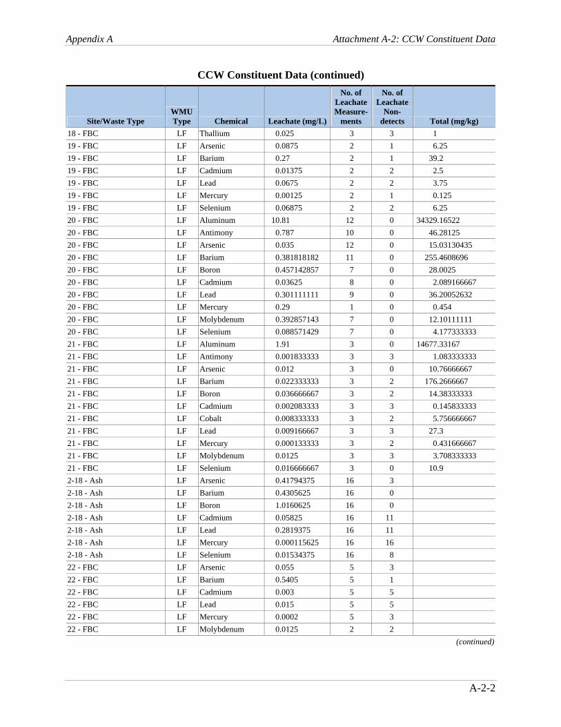
Appendix A Attachment A-2: CCW Constituent Data
A-2-2
CCW Constituent Data (continued)
Site/Waste Type WMU Type Chemical Leachate (mg/L)
No. of Leachate Measure-
ments
No. of Leachate
Non-detects Total (mg/kg)
18 - FBC LF Thallium 0.025 3 3 1 19 - FBC LF Arsenic 0.0875 2 1 6.25 19 - FBC LF Barium 0.27 2 1 39.2 19 - FBC LF Cadmium 0.01375 2 2 2.5 19 - FBC LF Lead 0.0675 2 2 3.75 19 - FBC LF Mercury 0.00125 2 1 0.125 19 - FBC LF Selenium 0.06875 2 2 6.25 20 - FBC LF Aluminum 10.81 12 0 34329.16522 20 - FBC LF Antimony 0.787 10 0 46.28125 20 - FBC LF Arsenic 0.035 12 0 15.03130435 20 - FBC LF Barium 0.381818182 11 0 255.4608696 20 - FBC LF Boron 0.457142857 7 0 28.0025 20 - FBC LF Cadmium 0.03625 8 0 2.089166667 20 - FBC LF Lead 0.301111111 9 0 36.20052632 20 - FBC LF Mercury 0.29 1 0 0.454 20 - FBC LF Molybdenum 0.392857143 7 0 12.10111111 20 - FBC LF Selenium 0.088571429 7 0 4.177333333 21 - FBC LF Aluminum 1.91 3 0 14677.33167 21 - FBC LF Antimony 0.001833333 3 3 1.083333333 21 - FBC LF Arsenic 0.012 3 0 10.76666667 21 - FBC LF Barium 0.022333333 3 2 176.2666667 21 - FBC LF Boron 0.036666667 3 2 14.38333333 21 - FBC LF Cadmium 0.002083333 3 3 0.145833333 21 - FBC LF Cobalt 0.008333333 3 2 5.756666667 21 - FBC LF Lead 0.009166667 3 3 27.3 21 - FBC LF Mercury 0.000133333 3 2 0.431666667 21 - FBC LF Molybdenum 0.0125 3 3 3.708333333 21 - FBC LF Selenium 0.016666667 3 0 10.9 2-18 - Ash LF Arsenic 0.41794375 16 3 2-18 - Ash LF Barium 0.4305625 16 0 2-18 - Ash LF Boron 1.0160625 16 0 2-18 - Ash LF Cadmium 0.05825 16 11 2-18 - Ash LF Lead 0.2819375 16 11 2-18 - Ash LF Mercury 0.000115625 16 16 2-18 - Ash LF Selenium 0.01534375 16 8 22 - FBC LF Arsenic 0.055 5 3 22 - FBC LF Barium 0.5405 5 1 22 - FBC LF Cadmium 0.003 5 5 22 - FBC LF Lead 0.015 5 5 22 - FBC LF Mercury 0.0002 5 3 22 - FBC LF Molybdenum 0.0125 2 2
(continued)

Appendix A Attachment A-2: CCW Constituent Data
A-2-3
CCW Constituent Data (continued)
Site/Waste Type WMU Type Chemical Leachate (mg/L)
No. of Leachate Measure-
ments
No. of Leachate
Non-detects Total (mg/kg)
22 - FBC LF Selenium 0.032 5 5 23 - FBC LF Barium 0.81 4 0 25 - FBC LF Arsenic 0.125 1 1 25 - FBC LF Barium 2.5 1 1 25 - FBC LF Cadmium 0.025 1 1 25 - FBC LF Lead 0.125 1 1 25 - FBC LF Mercury 0.005 1 1 25 - FBC LF Selenium 0.025 1 1 28 - FBC LF Barium 2.525 2 0 235.11875 30 - FBC LF Aluminum 6.894555556 18 7 28246.46923 30 - FBC LF Antimony 0.548082353 17 2 61.49315385 30 - FBC LF Arsenic 0.050694444 18 3 48.55980769 30 - FBC LF Barium 0.286388889 18 6 120.0687692 30 - FBC LF Boron 0.31759375 16 7 30.83913462 30 - FBC LF Cadmium 0.023125 14 3 1.916230769 30 - FBC LF Lead 0.240805556 18 4 39.36092308 30 - FBC LF Mercury 0.000744444 18 17 10.91689923 30 - FBC LF Molybdenum 0.138125 16 10 14.50257692 30 - FBC LF Selenium 0.10475 16 10 5.603596154 31 - FBC LF Aluminum 0.28 1 0 29437.5 31 - FBC LF Antimony 0.00065 1 1 5.0325 31 - FBC LF Arsenic 0.0687 4 2 26.825 31 - FBC LF Barium 0.58275 4 0 170.25 31 - FBC LF Boron 26.7 1 0 930 31 - FBC LF Cadmium 0.02775 4 3 5.45 31 - FBC LF Cobalt 0.0065 1 0 6.42 31 - FBC LF Lead 0.03025 4 3 1.19 31 - FBC LF Mercury 0.00095 4 1 0.61 31 - FBC LF Molybdenum 0.085 1 0 8 31 - FBC LF Selenium 0.06485 4 2 7.54 32 - FBC LF Arsenic 0.35 1 1 1.4 32 - FBC LF Barium 0.085 1 0 32 - FBC LF Cadmium 0.005 1 1 0.009 32 - FBC LF Lead 0.05 1 1 0.45 32 - FBC LF Mercury 0.0001 1 1 0.03 32 - FBC LF Selenium 0.175 1 1 3.5 33 - FBC LF Arsenic 0.015 1 1 33 - FBC LF Barium 42 1 0 33 - FBC LF Boron 0.06 1 0 33 - FBC LF Cadmium 0.00125 1 1 33 - FBC LF Cobalt 0.0025 1 1 33 - FBC LF Mercury 0.00005 1 1
(continued)
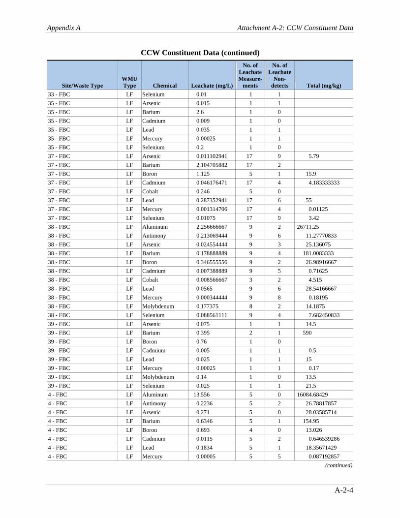
Appendix A Attachment A-2: CCW Constituent Data
A-2-4
CCW Constituent Data (continued)
Site/Waste Type WMU Type Chemical Leachate (mg/L)
No. of Leachate Measure-
ments
No. of Leachate
Non-detects Total (mg/kg)
33 - FBC LF Selenium 0.01 1 1 35 - FBC LF Arsenic 0.015 1 1 35 - FBC LF Barium 2.6 1 0 35 - FBC LF Cadmium 0.009 1 0 35 - FBC LF Lead 0.035 1 1 35 - FBC LF Mercury 0.00025 1 1 35 - FBC LF Selenium 0.2 1 0 37 - FBC LF Arsenic 0.011102941 17 9 5.79 37 - FBC LF Barium 2.104705882 17 2 37 - FBC LF Boron 1.125 5 1 15.9 37 - FBC LF Cadmium 0.046176471 17 4 4.183333333 37 - FBC LF Cobalt 0.246 5 0 37 - FBC LF Lead 0.287352941 17 6 55 37 - FBC LF Mercury 0.001314706 17 4 0.01125 37 - FBC LF Selenium 0.01075 17 9 3.42 38 - FBC LF Aluminum 2.256666667 9 2 26711.25 38 - FBC LF Antimony 0.213069444 9 6 11.27770833 38 - FBC LF Arsenic 0.024554444 9 3 25.136075 38 - FBC LF Barium 0.178888889 9 4 181.0083333 38 - FBC LF Boron 0.346555556 9 2 26.98916667 38 - FBC LF Cadmium 0.007388889 9 5 0.71625 38 - FBC LF Cobalt 0.008566667 3 2 4.515 38 - FBC LF Lead 0.0565 9 6 28.54166667 38 - FBC LF Mercury 0.000344444 9 8 0.18195 38 - FBC LF Molybdenum 0.177375 8 2 14.1875 38 - FBC LF Selenium 0.088561111 9 4 7.682450833 39 - FBC LF Arsenic 0.075 1 1 14.5 39 - FBC LF Barium 0.395 2 1 590 39 - FBC LF Boron 0.76 1 0 39 - FBC LF Cadmium 0.005 1 1 0.5 39 - FBC LF Lead 0.025 1 1 15 39 - FBC LF Mercury 0.00025 1 1 0.17 39 - FBC LF Molybdenum 0.14 1 0 13.5 39 - FBC LF Selenium 0.025 1 1 21.5 4 - FBC LF Aluminum 13.556 5 0 16084.68429 4 - FBC LF Antimony 0.2236 5 2 26.78817857 4 - FBC LF Arsenic 0.271 5 0 28.03585714 4 - FBC LF Barium 0.6346 5 1 154.95 4 - FBC LF Boron 0.693 4 0 13.026 4 - FBC LF Cadmium 0.0115 5 2 0.646539286 4 - FBC LF Lead 0.1834 5 1 18.35671429 4 - FBC LF Mercury 0.00005 5 5 0.087192857
(continued)

Appendix A Attachment A-2: CCW Constituent Data
A-2-5
CCW Constituent Data (continued)
Site/Waste Type WMU Type Chemical Leachate (mg/L)
No. of Leachate Measure-
ments
No. of Leachate
Non-detects Total (mg/kg)
4 - FBC LF Molybdenum 0.286666667 3 0 16.18257143 4 - FBC LF Selenium 0.0620625 4 2 1.505421429 41 - FBC LF Antimony 0.025 5 5 1.551333333 41 - FBC LF Arsenic 0.035471698 53 50 13.72255319 41 - FBC LF Barium 0.095694444 54 25 19.05490196 41 - FBC LF Cadmium 0.022355769 52 51 0.427826087 41 - FBC LF Lead 0.017548077 52 51 0.935208333 41 - FBC LF Mercury 0.000596154 52 50 0.119542553 41 - FBC LF Selenium 0.024433962 53 51 1.505744681 41 - FBC LF Thallium 0.031 5 4 3.662790698 42 - FBC LF Arsenic 0.0125 2 2 42 - FBC LF Barium 0.1625 2 1 42 - FBC LF Cadmium 0.005 2 2 42 - FBC LF Lead 0.0075 2 2 42 - FBC LF Mercury 0.0005 2 2 42 - FBC LF Selenium 0.0125 2 2 43 - FBC LF Arsenic 0.0125 2 2 43 - FBC LF Barium 0.0875 2 1 43 - FBC LF Cadmium 0.005 2 2 43 - FBC LF Lead 0.0075 2 2 43 - FBC LF Mercury 0.0005 2 2 43 - FBC LF Selenium 0.08625 2 1 6 - FBC LF Aluminum 0.1525 2 1 42736.5 6 - FBC LF Antimony 0.05 2 2 16.25 6 - FBC LF Arsenic 0.09125 2 1 126.6 6 - FBC LF Barium 0.285 2 0 221.5 6 - FBC LF Boron 0.1425 2 1 73.8 6 - FBC LF Cadmium 0.0025 2 2 1.29625 6 - FBC LF Lead 0.01375 2 2 8.1125 6 - FBC LF Mercury 0.00005 2 2 1.16 6 - FBC LF Molybdenum 0.09 2 0 1.425 6 - FBC LF Selenium 0.1025 2 1 84.5625 Amerikohl - FBC LF Aluminum 0.753333333 3 0 51600 Amerikohl - FBC LF Antimony 0.345 3 3 20 Amerikohl - FBC LF Arsenic 0.024166667 3 3 114 Amerikohl - FBC LF Barium 0.1 3 3 140 Amerikohl - FBC LF Boron 0.346666667 3 1 60 Amerikohl - FBC LF Cadmium 0.004166667 3 3 0.15 Amerikohl - FBC LF Cobalt 0.175 3 3 30 Amerikohl - FBC LF Lead 0.009166667 3 3 23 Amerikohl - FBC LF Mercury 0.0005 3 3 0.15 Amerikohl - FBC LF Molybdenum 0.266666667 3 1 10
(continued)

Appendix A Attachment A-2: CCW Constituent Data
A-2-6
CCW Constituent Data (continued)
Site/Waste Type WMU Type Chemical Leachate (mg/L)
No. of Leachate Measure-
ments
No. of Leachate
Non-detects Total (mg/kg)
Amerikohl - FBC LF Nitrate/Nitrite 3.15 3 3 Amerikohl - FBC LF Selenium 0.044166667 3 3 3.5 Arkwright - Ash LF Arsenic 0.07 1 0 Arkwright - Ash LF Barium 0.4 1 0 Arkwright - Ash LF Cadmium 0.01 1 0 Arkwright - Ash LF Lead 0.04 1 0 Arkwright - Ash LF Selenium 0.02 1 0 Barry - Ash LF Arsenic 1 1 0 Barry - Ash LF Barium 0.7 1 0 Barry - Ash LF Cadmium 0.005 1 0 Barry - Ash LF Lead 0.04 1 0 Barry - Ash LF Selenium 0.07 1 0 Belle Ayr - Ash LF Aluminum 0.036666667 3 0 Belle Ayr - Ash LF Antimony 0.021 2 0 Belle Ayr - Ash LF Arsenic 0.181 3 0 Belle Ayr - Ash LF Barium 1.163333333 3 0 Belle Ayr - Ash LF Cobalt 0.0075 2 0 Belle Ayr - Ash LF Molybdenum 0.325 3 0 Belle Ayr - Ash LF Selenium 0.652333333 3 0 Big Gorilla Pit - FBC LF Aluminum 3.774166667 12 0 18440.58824 Big Gorilla Pit - FBC LF Antimony 0.037166667 12 1 1.244485294 Big Gorilla Pit - FBC LF Arsenic 0.023181818 22 21 7.534117647 Big Gorilla Pit - FBC LF Barium 0.243636364 11 3 147.7320588 Big Gorilla Pit - FBC LF Boron 0.677916667 12 2 29.64058824 Big Gorilla Pit - FBC LF Cadmium 0.015227273 22 22 0.58728125 Big Gorilla Pit - FBC LF Cobalt 0.008553571 14 11 2.374214286 Big Gorilla Pit - FBC LF Lead 0.08125 12 7 19.51823529 Big Gorilla Pit - FBC LF Mercury 0.001704545 22 19 0.302990909 Big Gorilla Pit - FBC LF Molybdenum 0.1202 10 1 6.429333333 Big Gorilla Pit - FBC LF Nitrate/Nitrite 1.755857143 14 3 Big Gorilla Pit - FBC LF Selenium 0.10975 12 1 7.159397059 Bowen - Ash LF Arsenic 0.6 1 0 68 Bowen - Ash LF Barium 0.3 1 0 974 Bowen - Ash LF Cadmium 0.01 1 0 0.7 Bowen - Ash LF Lead 0.04 1 0 63.9 Bowen - Ash LF Selenium 0.1 1 0 Branch - Ash LF Arsenic 0.04 1 0 Branch - Ash LF Barium 0.5 1 0 Branch - Ash LF Cadmium 0.01 1 0 Branch - Ash LF Lead 0.04 1 0 Branch - Ash LF Selenium 0.06 1 0 Buckheart Mine - Ash LF Antimony 0.01854 40 14
(continued)

Appendix A Attachment A-2: CCW Constituent Data
A-2-7
CCW Constituent Data (continued)
Site/Waste Type WMU Type Chemical Leachate (mg/L)
No. of Leachate Measure-
ments
No. of Leachate
Non-detects Total (mg/kg)
Buckheart Mine - Ash LF Arsenic 0.122357143 42 13 Buckheart Mine - Ash LF Barium 0.364809524 42 0 Buckheart Mine - Ash LF Boron 9.998738095 42 0 Buckheart Mine - Ash LF Cadmium 0.0235 42 8 Buckheart Mine - Ash LF Cobalt 0.048047619 42 17 Buckheart Mine - Ash LF Lead 0.27887619 42 9 Buckheart Mine - Ash LF Mercury 0.000107143 42 40 Buckheart Mine - Ash LF Selenium 0.118266667 42 26 Buckheart Mine - Ash LF Thallium 0.017875 40 10 Buckheart Mine - FBC LF Antimony 0.0018125 8 8 Buckheart Mine - FBC LF Arsenic 0.0465 8 5 Buckheart Mine - FBC LF Barium 0.560125 8 1 Buckheart Mine - FBC LF Boron 3.157 8 0 Buckheart Mine - FBC LF Cadmium 0.0033125 8 7 Buckheart Mine - FBC LF Cobalt 0.02875 8 7 Buckheart Mine - FBC LF Lead 0.036 8 4 Buckheart Mine - FBC LF Mercury 0.0005 8 4 Buckheart Mine - FBC LF Selenium 0.050625 8 5 Buckheart Mine - FBC LF Thallium 0.001 8 8 CAER - Ash LF Arsenic 1.132 5 0 77.32222222 CAER - Ash LF Barium 0.315 5 0 537.6666667 CAER - Ash LF Cadmium 0.0942 5 0 CAER - Ash LF Lead 0.1 5 2 73.62375 CAER - Ash LF Mercury 0.00025 5 5 CAER - Ash LF Selenium 0.103 5 0 Canton Site - Ash LF Aluminum 9.818127778 36 0 Canton Site - Ash LF Arsenic 0.0025 2 2 Canton Site - Ash LF Barium 3.0156 10 0 Canton Site - Ash LF Boron 18.62468571 35 0 Canton Site - Ash LF Cadmium 0.0005 2 2 Canton Site - Ash LF Cobalt 0.02 1 1 Canton Site - Ash LF Lead 0.1865 2 0 Canton Site - Ash LF Mercury 0.0001 1 1 Canton Site - Ash LF Molybdenum 30.9359 20 0 Canton Site - Ash LF Nitrate/Nitrite 0.095 1 0 Canton Site - Ash LF Selenium 0.0374 1 0 Canton Site - FBC LF Aluminum 2.461866667 24 0 Canton Site - FBC LF Arsenic 0.005 1 1 Canton Site - FBC LF Barium 0.02 1 0 Canton Site - FBC LF Boron 1.5602625 16 0 Canton Site - FBC LF Cadmium 0.066 1 0 Canton Site - FBC LF Lead 0.062 1 0
(continued)

Appendix A Attachment A-2: CCW Constituent Data
A-2-8
CCW Constituent Data (continued)
Site/Waste Type WMU Type Chemical Leachate (mg/L)
No. of Leachate Measure-
ments
No. of Leachate
Non-detects Total (mg/kg)
Canton Site – FBC LF Mercury 0.0005 1 1 Canton Site – FBC LF Molybdenum 1.768009524 21 0 Canton Site – FBC LF Selenium 0.005 1 1 Central Cleaning Plant - Ash LF Antimony 0.008205882 17 17 Central Cleaning Plant - Ash LF Arsenic 0.005 17 17 Central Cleaning Plant - Ash LF Barium 0.168164706 17 0 Central Cleaning Plant - Ash LF Boron 7.213823529 17 0 Central Cleaning Plant - Ash LF Cadmium 0.004117647 17 16 Central Cleaning Plant - Ash LF Cobalt 0.019588235 17 15 Central Cleaning Plant - Ash LF Lead 0.022782353 17 11 Central Cleaning Plant - Ash LF Mercury 0.000568824 17 11 Central Cleaning Plant - Ash LF Selenium 0.040211765 17 0 Central Cleaning Plant - Ash LF Thallium 0.005 17 17 CL - Ash and Coal Refuse LF Aluminum 2.58 3 0 CL - Ash and Coal Refuse LF Antimony 0.0041 3 0 CL - Ash and Coal Refuse LF Arsenic 0.121266667 3 0 CL - Ash and Coal Refuse LF Barium 3.63 3 0 CL - Ash and Coal Refuse LF Boron 0.103133333 3 0 CL - Ash and Coal Refuse LF Cadmium 0.001 3 0 CL - Ash and Coal Refuse LF Cobalt 0.006066667 3 1 CL - Ash and Coal Refuse LF Lead 0.003533333 3 0 CL - Ash and Coal Refuse LF Mercury 0.00005 6 6 CL - Ash and Coal Refuse LF Selenium 0.0452 3 0 CL - Ash and Coal Refuse LF Thallium 0.003483333 3 1 Coal Creek - Ash LF Arsenic 0.0109 2 0 0.086 Coal Creek - Ash LF Barium 0.6105 2 0 4.76 Coal Creek - Ash LF Boron 6.22 2 0 1.1105 Coal Creek - Ash LF Cadmium 0.00015 2 2 0.00045 Coal Creek - Ash LF Lead 0.001 2 2 0.02025 Coal Creek - Ash LF Mercury 0.000005 2 2 0.0006 Coal Creek - Ash LF Selenium 0.0555 2 1 0.00505 Colver Site - FBC LF Aluminum 0.248333333 6 1 78878.83333 Colver Site - FBC LF Antimony 0.196666667 6 2 166.5 Colver Site - FBC LF Arsenic 0.0875 6 1 124.2 Colver Site - FBC LF Barium 0.291666667 6 0 443.8333333 Colver Site - FBC LF Boron 0.261666667 6 1 62.6 Colver Site - FBC LF Cadmium 0.016666667 6 2 9.994166667 Colver Site - FBC LF Lead 0.190833333 6 2 192.075 Colver Site - FBC LF Mercury 0.00015 6 5 0.586666667 Colver Site - FBC LF Molybdenum 0.143333333 6 0 30.65833333 Colver Site - FBC LF Selenium 0.48 6 1 68.70833333 Conemaugh - Ash LF Aluminum 1.245 2 0
(continued)

Appendix A Attachment A-2: CCW Constituent Data
A-2-9
CCW Constituent Data (continued)
Site/Waste Type WMU Type Chemical Leachate (mg/L)
No. of Leachate Measure-
ments
No. of Leachate
Non-detects Total (mg/kg)
Conemaugh - Ash LF Antimony 0.075 1 1 Conemaugh - Ash LF Arsenic 0.388333333 3 1 Conemaugh - Ash LF Barium 0.331666667 3 0 Conemaugh - Ash LF Boron 0.91 1 0 Conemaugh - Ash LF Cadmium 0.01 3 0 Conemaugh - Ash LF Cobalt 0.026 1 0 Conemaugh - Ash LF Lead 0.1 2 2 Conemaugh - Ash LF Mercury 0.00055 2 2 Conemaugh - Ash LF Molybdenum 0.355 2 0 Conemaugh - Ash LF Selenium 0.295 2 1 Conemaugh - Ash LF Thallium 0.024 1 0 Conemaugh - Ash and Coal Refuse
LF Aluminum 1.467666667 3 0
Conemaugh - Ash and Coal Refuse
LF Antimony 0.075 3 3
Conemaugh - Ash and Coal Refuse
LF Arsenic 0.625 2 2
Conemaugh - Ash and Coal Refuse
LF Barium 0.145666667 3 0
Conemaugh - Ash and Coal Refuse
LF Boron 0.095 2 0
Conemaugh - Ash and Coal Refuse
LF Cadmium 0.002 3 3
Conemaugh - Ash and Coal Refuse
LF Cobalt 0.009 1 0
Conemaugh - Ash and Coal Refuse
LF Lead 0.073333333 3 2
Conemaugh - Ash and Coal Refuse
LF Mercury 0.0004 3 2
Conemaugh - Ash and Coal Refuse
LF Molybdenum 0.01 1 0
Conemaugh - Ash and Coal Refuse
LF Selenium 0.179833333 3 1
Conemaugh - Ash and Coal Refuse
LF Thallium 0.005 1 0
Crist - Ash LF Arsenic 0.02 1 0 Crist - Ash LF Barium 0.1 1 0 Crist - Ash LF Cadmium 0.02 1 0 Crist - Ash LF Lead 0.003 1 0 Crist - Ash LF Selenium 0.05 1 0 Crown III - Ash LF Antimony 0.071159259 54 10 Crown III - Ash LF Arsenic 0.352503226 62 29 Crown III - Ash LF Barium 0.279112903 62 3 Crown III - Ash LF Boron 22.93277419 62 0
(continued)

Appendix A Attachment A-2: CCW Constituent Data
A-2-10
CCW Constituent Data (continued)
Site/Waste Type WMU Type Chemical Leachate (mg/L)
No. of Leachate Measure-
ments
No. of Leachate
Non-detects Total (mg/kg)
Crown III - Ash LF Cadmium 0.128258065 62 3 Crown III - Ash LF Cobalt 0.101225806 62 17 Crown III - Ash LF Lead 0.605616935 62 19 Crown III - Ash LF Mercury 0.000104839 62 61 Crown III - Ash LF Molybdenum 0.588888889 9 4 Crown III - Ash LF Selenium 0.03946129 62 46 Crown III - Ash LF Thallium 0.0645 54 18 Crown III - FBC LF Antimony 0.0135 17 9 Crown III - FBC LF Arsenic 0.034822581 31 26 3.766666667 Crown III - FBC LF Barium 0.346774194 31 2 150 Crown III - FBC LF Boron 2.815296296 27 1 Crown III - FBC LF Cadmium 0.011241935 31 22 2.17 Crown III - FBC LF Cobalt 0.02475 24 16 Crown III - FBC LF Lead 0.068645161 31 17 8.233333333 Crown III - FBC LF Mercury 0.000164516 31 27 0.381 Crown III - FBC LF Molybdenum 0.1522 10 2 Crown III - FBC LF Selenium 0.061467742 31 27 3.3 Crown III - FBC LF Thallium 0.004941176 17 11 CTL-V - Ash LF Antimony 0.26 1 0 CTL-V - Ash LF Arsenic 0.037 1 0 CTL-V - Ash LF Barium 0.247 1 0 CTL-V - Ash LF Cadmium 0.04 1 0 CTL-V - Ash LF Lead 0.072 1 0 CTL-V - Ash LF Mercury 0.001 1 0 CTL-V - Ash LF Selenium 0.014 1 0 CTL-V - Ash LF Thallium 0.01 1 0 CY - Ash LF Aluminum 4.735 2 0 CY - Ash LF Antimony 0.0078 2 0 CY - Ash LF Arsenic 0.04825 2 0 CY - Ash LF Barium 1.2395 2 0 CY - Ash LF Boron 6.13 2 0 CY - Ash LF Cadmium 0.0002075 2 1 CY - Ash LF Cobalt 0.001915 4 4 CY - Ash LF Lead 0.003555 2 1 CY - Ash LF Mercury 0.000265 2 0 CY - Ash LF Selenium 0.004825 2 1 CY - Ash LF Thallium 0.00196 4 4 Dairyland Power Coop - Ash LF Arsenic 0.0328625 8 0 Dairyland Power Coop - Ash LF Barium 0.058740741 27 0 Dairyland Power Coop - Ash LF Boron 68.03979592 49 0 Dairyland Power Coop - Ash LF Cadmium 0.00539 34 0 Dairyland Power Coop - Ash LF Lead 0.0046 7 2
(continued)

Appendix A Attachment A-2: CCW Constituent Data
A-2-11
CCW Constituent Data (continued)
Site/Waste Type WMU Type Chemical Leachate (mg/L)
No. of Leachate Measure-
ments
No. of Leachate
Non-detects Total (mg/kg)
Dairyland Power Coop - Ash LF Mercury 0.000223 2 1 Dairyland Power Coop - Ash LF Selenium 0.0696375 8 0 Daniel - Ash LF Arsenic 0.2 1 0 Daniel - Ash LF Barium 0.4 1 0 Daniel - Ash LF Cadmium 0.001 1 1 Daniel - Ash LF Lead 0.001 1 1 Daniel - Ash LF Selenium 0.001 1 1 Deer Ridge Mine - Ash LF Aluminum 0.5941 10 1 64681.487 Deer Ridge Mine - Ash LF Arsenic 0.0029 10 6 21.29419 Deer Ridge Mine - Ash LF Barium 0.1448 10 2 258.468 Deer Ridge Mine - Ash LF Boron 1.228 10 2 179.354 Deer Ridge Mine - Ash LF Cadmium 0.01365 10 1 0.94425 Deer Ridge Mine - Ash LF Lead 0.0253 10 2 58.48 Deer Ridge Mine - Ash LF Mercury 0.00011025 10 10 0.1158 Deer Ridge Mine - Ash LF Molybdenum 0.0756 10 4 6.6287 Deer Ridge Mine - Ash LF Nitrate/Nitrite 0.095 3 2 Deer Ridge Mine - Ash LF Selenium 0.01022 10 2 13.1061 DPC - Ash LF Antimony 0.04 2 1 0.475 DPC - Ash LF Arsenic 0.051 2 0 55.085 DPC - Ash LF Barium 0.28 2 0 37.7 DPC - Ash LF Boron 27.945 2 0 404.05 DPC - Ash LF Cadmium 0.005 4 4 0.56 DPC - Ash LF Lead 0.025 4 4 28.7 DPC - Ash LF Mercury 0.001 2 2 0.127 DPC - Ash LF Nitrate/Nitrite 2.5 2 0 0.2425 DPC - Ash LF Selenium 0.046 2 0 3.4445 EERC - Ash LF Mercury 0.000025 4 4 Elkhart Mine - Ash LF Antimony 0.025192308 52 46 Elkhart Mine - Ash LF Arsenic 0.043571429 77 71 Elkhart Mine - Ash LF Barium 0.495324675 77 23 Elkhart Mine - Ash LF Boron 6.88961039 77 0 Elkhart Mine - Ash LF Cadmium 0.022551948 77 41 Elkhart Mine - Ash LF Cobalt 0.012785714 77 57 Elkhart Mine - Ash LF Lead 0.027987013 77 66 Elkhart Mine - Ash LF Mercury 0.000148052 77 68 Elkhart Mine - Ash LF Selenium 0.036649351 77 64 Elkhart Mine - Ash LF Thallium 0.015942308 52 48 Elkhart Mine - FBC LF Antimony 0.021875 16 15 Elkhart Mine - FBC LF Arsenic 0.034512195 41 37 Elkhart Mine - FBC LF Barium 0.525365854 41 5 Elkhart Mine - FBC LF Boron 13.13829268 41 0 Elkhart Mine - FBC LF Cadmium 0.003536585 41 41
(continued)

Appendix A Attachment A-2: CCW Constituent Data
A-2-12
CCW Constituent Data (continued)
Site/Waste Type WMU Type Chemical Leachate (mg/L)
No. of Leachate Measure-
ments
No. of Leachate
Non-detects Total (mg/kg)
Elkhart Mine - FBC LF Cobalt 0.007219512 41 39 Elkhart Mine - FBC LF Lead 0.017195122 41 34 Elkhart Mine - FBC LF Mercury 0.000104878 41 40 Elkhart Mine - FBC LF Selenium 0.035365854 41 33 Elkhart Mine - FBC LF Thallium 0.02390625 16 15 FBX - Ash LF Arsenic 0.0025 2 2 FBX - Ash LF Barium 29.6225 2 1 FBX - Ash LF Cadmium 0.2 2 2 FBX - Ash LF Lead 0.5 2 2 FBX - Ash LF Mercury 0.00025 2 2 FBX - Ash LF Selenium 0.01375 2 2 FC - Ash and Coal Refuse LF Aluminum 13.8 2 0 FC - Ash and Coal Refuse LF Antimony 0.00105 4 4 FC - Ash and Coal Refuse LF Arsenic 0.005 2 0 FC - Ash and Coal Refuse LF Barium 0.602 2 0 FC - Ash and Coal Refuse LF Boron 2.54 2 0 FC - Ash and Coal Refuse LF Cadmium 0.00015 4 4 FC - Ash and Coal Refuse LF Cobalt 0.0029 2 0 FC - Ash and Coal Refuse LF Lead 0.00345 2 0 FC - Ash and Coal Refuse LF Mercury 0.00005 4 4 FC - Ash and Coal Refuse LF Selenium 0.01765 2 0 FC - Ash and Coal Refuse LF Thallium 0.00185 4 4 Florence Mine - Ash LF Aluminum 0.03 1 0 Florence Mine - Ash LF Antimony 0.005 1 1 Florence Mine - Ash LF Arsenic 0.07 1 0 Florence Mine - Ash LF Barium 2.23 1 0 Florence Mine - Ash LF Boron 0.01 1 1 Florence Mine - Ash LF Cadmium 0.01 1 1 Florence Mine - Ash LF Lead 0.001 1 0 Florence Mine - Ash LF Mercury 0.002 1 0 Florence Mine - Ash LF Molybdenum 0.01 1 1 Florence Mine - Ash LF Nitrate/Nitrite 1.2 1 0 Florence Mine - Ash LF Selenium 0.06 1 0 Fran Site - FBC LF Aluminum 0.32 1 0 Fran Site - FBC LF Antimony 0.005 1 1 Fran Site - FBC LF Arsenic 0.02 1 0 Fran Site - FBC LF Barium 0.08 1 0 Fran Site - FBC LF Boron 0.43 1 0 Fran Site - FBC LF Cadmium 0.005 1 1 Fran Site - FBC LF Lead 0.005 1 1 Fran Site - FBC LF Nitrate/Nitrite 1.22 1 0 Fran Site - FBC LF Selenium 0.03 1 0
(continued)

Appendix A Attachment A-2: CCW Constituent Data
A-2-13
CCW Constituent Data (continued)
Site/Waste Type WMU Type Chemical Leachate (mg/L)
No. of Leachate Measure-
ments
No. of Leachate
Non-detects Total (mg/kg)
FW - FBC LF Arsenic 0.02525 4 3 FW - FBC LF Barium 0.304 4 0 FW - FBC LF Cadmium 0.005 4 4 FW - FBC LF Lead 0.05 4 4 FW - FBC LF Mercury 0.001 4 4 FW - FBC LF Selenium 0.1 4 4 Gadsden - Ash LF Arsenic 0.2 1 0 Gadsden - Ash LF Barium 0.3 1 0 Gadsden - Ash LF Cadmium 0.01 1 0 Gadsden - Ash LF Lead 0.04 1 0 Gadsden - Ash LF Selenium 0.03 1 0 Gale - Ash LF Aluminum 3.1 1 0 13630 Gale - Ash LF Antimony 0.03 1 0 3 Gale - Ash LF Arsenic 0.42 1 0 51.5 Gale - Ash LF Barium 1.7 1 0 143 Gale - Ash LF Boron 0.22 1 0 25 Gale - Ash LF Cadmium 0.01 1 0 1 Gale - Ash LF Lead 0.23 1 0 21 Gale - Ash LF Molybdenum 0.05 1 0 5 Gale - Ash LF Selenium 0.1 1 0 4.4 Gaston - Ash LF Arsenic 1.8 1 0 Gaston - Ash LF Barium 0.3 1 0 Gaston - Ash LF Cadmium 0.01 1 0 Gaston - Ash LF Lead 0.05 1 0 Gaston - Ash LF Selenium 0.003 1 0 Gorgas - Ash LF Arsenic 1.6 1 0 Gorgas - Ash LF Barium 0.3 1 0 Gorgas - Ash LF Cadmium 0.01 1 0 Gorgas - Ash LF Lead 0.04 1 0 Gorgas - Ash LF Selenium 0.002 1 0 Greene Co - Ash LF Arsenic 1.1 1 0 Greene Co - Ash LF Barium 0.4 1 0 Greene Co - Ash LF Cadmium 0.01 1 0 Greene Co - Ash LF Lead 0.04 1 0 Greene Co - Ash LF Selenium 0.003 1 0 HA - Ash and Coal Refuse LF Aluminum 1.71925 4 0 5666.666667 HA - Ash and Coal Refuse LF Antimony 0.003905 4 2 HA - Ash and Coal Refuse LF Arsenic 0.024975 4 0 9.666666667 HA - Ash and Coal Refuse LF Barium 1.01675 4 0 186.6666667 HA - Ash and Coal Refuse LF Boron 0.64545 4 0 14 HA - Ash and Coal Refuse LF Cadmium 0.0039275 4 0 0.25 HA - Ash and Coal Refuse LF Cobalt 0.01517875 4 1
(continued)

Appendix A Attachment A-2: CCW Constituent Data
A-2-14
CCW Constituent Data (continued)
Site/Waste Type WMU Type Chemical Leachate (mg/L)
No. of Leachate Measure-
ments
No. of Leachate
Non-detects Total (mg/kg)
HA - Ash and Coal Refuse LF Lead 0.00378 4 2 8.7 HA - Ash and Coal Refuse LF Mercury 0.0001 4 0 0.065 HA - Ash and Coal Refuse LF Selenium 0.005025 4 0 0.534166667 HA - Ash and Coal Refuse LF Thallium 0.00196 8 8 Hammond - Ash LF Arsenic 0.1 1 0 Hammond - Ash LF Barium 0.3 1 0 Hammond - Ash LF Cadmium 0.01 1 0 Hammond - Ash LF Lead 0.05 1 0 Hammond - Ash LF Selenium 0.02 1 0 Harrim 3019 - Ash LF Aluminum 5.21 1 0 46577 Harrim 3019 - Ash LF Antimony 0.0058 1 0 646.4 Harrim 3019 - Ash LF Arsenic 0.178 1 0 50.43172727 Harrim 3019 - Ash LF Barium 0.32 1 0 319.89 Harrim 3019 - Ash LF Molybdenum 0.594 1 0 17.9 Harrim 3019 - Ash LF Nitrate/Nitrite 1.99 1 0 Harrim 3019 - Ash LF Selenium 0.0468 1 0 1.405714286 Harrim 3019 - FBC LF Aluminum 0.67375 8 0 Harrim 3019 - FBC LF Antimony 0.002 1 0 Harrim 3019 - FBC LF Barium 0.465888889 9 0 Harrim 3019 - FBC LF Boron 0.07 1 0 Harrim 3019 - FBC LF Cobalt 0.1385 6 0 Harrim 3019 - FBC LF Lead 0.24 5 0 Harrim 3019 - FBC LF Molybdenum 0.347714286 7 0 Harrim 3019 - FBC LF Nitrate/Nitrite 0.199333333 3 0 Harrim 3019 - FBC LF Selenium 0.019 2 0 Industry Mine - Ash LF Antimony 0.031597143 70 12 Industry Mine - Ash LF Arsenic 0.050248454 97 51 Industry Mine - Ash LF Barium 0.328329897 97 13 Industry Mine - Ash LF Boron 4.719969072 97 0 Industry Mine - Ash LF Cadmium 0.059061856 97 7 Industry Mine - Ash LF Cobalt 0.120010309 97 30 Industry Mine - Ash LF Lead 3.610544845 97 16 Industry Mine - Ash LF Mercury 0.000284536 97 92 Industry Mine - Ash LF Selenium 0.052408247 97 64 Industry Mine - Ash LF Thallium 0.016984286 70 12 Industry Mine - FBC LF Antimony 0.017077778 9 4 Industry Mine - FBC LF Arsenic 0.031111111 9 7 Industry Mine - FBC LF Barium 9.515666667 9 0 Industry Mine - FBC LF Boron 2.813888889 9 2 Industry Mine - FBC LF Cadmium 0.015888889 9 7 Industry Mine - FBC LF Cobalt 0.029333333 9 8 Industry Mine - FBC LF Lead 0.051877778 9 6
(continued)

Appendix A Attachment A-2: CCW Constituent Data
A-2-15
CCW Constituent Data (continued)
Site/Waste Type WMU Type Chemical Leachate (mg/L)
No. of Leachate Measure-
ments
No. of Leachate
Non-detects Total (mg/kg)
Industry Mine - FBC LF Mercury 0.000222222 9 8 Industry Mine - FBC LF Selenium 0.080388889 9 4 Industry Mine - FBC LF Thallium 0.002288889 9 6 Key West - Ash LF Arsenic 0.005 1 1 Key West - Ash LF Barium 1 2 0 Key West - Ash LF Boron 0.2 1 0 Key West - Ash LF Cadmium 0.07 1 0 Key West - Ash LF Lead 0.4 1 0 Key West - Ash LF Mercury 0.18 1 0 Key West - Ash LF Selenium 0.005 1 1 Keystone - Ash LF Aluminum 2.059 4 0 Keystone - Ash LF Antimony 0.036 1 0 Keystone - Ash LF Arsenic 0.30925 4 0 Keystone - Ash LF Barium 0.40375 4 0 Keystone - Ash LF Boron 0.72 1 0 Keystone - Ash LF Cadmium 0.009625 4 1 Keystone - Ash LF Cobalt 0.023 1 0 Keystone - Ash LF Lead 0.045375 4 1 Keystone - Ash LF Mercury 0.001 1 1 Keystone - Ash LF Molybdenum 0.32 1 0 Keystone - Ash LF Selenium 0.0525 4 2 Keystone - Ash LF Thallium 0.083 1 0 Keystone - Ash and Coal Refuse
LF Aluminum 0.842 4 0
Keystone - Ash and Coal Refuse
LF Antimony 0.0015 2 2
Keystone - Ash and Coal Refuse
LF Arsenic 0.01875 4 4
Keystone - Ash and Coal Refuse
LF Barium 0.1925 4 0
Keystone - Ash and Coal Refuse
LF Boron 0.06 1 0
Keystone - Ash and Coal Refuse
LF Cadmium 0.00225 4 4
Keystone - Ash and Coal Refuse
LF Cobalt 0.022 1 0
Keystone - Ash and Coal Refuse
LF Lead 0.01875 4 4
Keystone - Ash and Coal Refuse
LF Mercury 0.001 1 1
Keystone - Ash and Coal Refuse
LF Molybdenum 0.01 2 2
(continued)

Appendix A Attachment A-2: CCW Constituent Data
A-2-16
CCW Constituent Data (continued)
Site/Waste Type WMU Type Chemical Leachate (mg/L)
No. of Leachate Measure-
ments
No. of Leachate
Non-detects Total (mg/kg)
Keystone - Ash and Coal Refuse
LF Selenium 0.02 4 4
Keystone - Ash and Coal Refuse
LF Thallium 0.028 1 0
Kraft - Ash LF Arsenic 0.02 1 0 Kraft - Ash LF Barium 0.3 1 0 Kraft - Ash LF Cadmium 0.01 1 0 Kraft - Ash LF Lead 0.04 1 0 Kraft - Ash LF Selenium 0.04 1 0 LIMB Site - Ash LF Aluminum 0.102894737 38 37 LIMB Site - Ash LF Antimony 0.29 5 1 25 LIMB Site - Ash LF Arsenic 0.033594737 38 6 63 LIMB Site - Ash LF Barium 0.036552632 38 0 255 LIMB Site - Ash LF Boron 0.521842105 38 31 400 LIMB Site - Ash LF Cadmium 0.001031579 38 33 0.31 LIMB Site - Ash LF Cobalt 0.005131579 38 37 LIMB Site - Ash LF Lead 0.012789474 38 25 14.5 LIMB Site - Ash LF Mercury 0.0001 2 2 LIMB Site - Ash LF Molybdenum 1.527342105 38 1 2.5 LIMB Site - Ash LF Nitrate/Nitrite 26 2 0 LIMB Site - Ash LF Selenium 0.0199 38 24 0.25 LIMB Site - Ash LF Thallium 0.05 5 5 Little Sandy #10 Mine - Ash LF Aluminum 1.078 6 2 4541.666667 Little Sandy #10 Mine - Ash LF Arsenic 0.032336364 11 8 38.293 Little Sandy #10 Mine - Ash LF Barium 0.264454545 11 6 48.81 Little Sandy #10 Mine - Ash LF Boron 2.630909091 11 3 157.76 Little Sandy #10 Mine - Ash LF Cadmium 0.008290909 11 9 1.198 Little Sandy #10 Mine - Ash LF Lead 0.022009091 11 10 56.84 Little Sandy #10 Mine - Ash LF Mercury 0.000486364 11 10 0.24435 Little Sandy #10 Mine - Ash LF Molybdenum 0.177272727 11 5 6.354 Little Sandy #10 Mine - Ash LF Selenium 0.059527273 11 9 6.531 Lone Mtn - Ash LF Aluminum 28.615 2 0 Lone Mtn - Ash LF Antimony 0.033 2 0 Lone Mtn - Ash LF Arsenic 0.185 2 0 76 Lone Mtn - Ash LF Barium 0.167 2 0 1483.2 Lone Mtn - Ash LF Cadmium 0.572 2 0 11.86 Lone Mtn - Ash LF Cobalt 0.142 2 0 87.3 Lone Mtn - Ash LF Mercury 0.0019 1 0 Lone Mtn - Ash LF Molybdenum 0.4295 2 0 Lone Mtn - Ash LF Selenium 0.328 2 0 LS - Ash and Coal Refuse LF Aluminum 1.18 7 0 LS - Ash and Coal Refuse LF Antimony 0.0107 4 0
(continued)
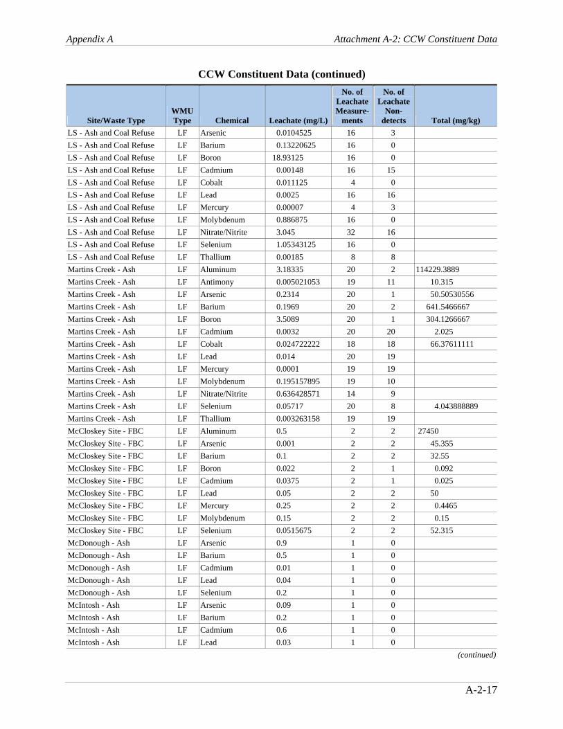
Appendix A Attachment A-2: CCW Constituent Data
A-2-17
CCW Constituent Data (continued)
Site/Waste Type WMU Type Chemical Leachate (mg/L)
No. of Leachate Measure-
ments
No. of Leachate
Non-detects Total (mg/kg)
LS - Ash and Coal Refuse LF Arsenic 0.0104525 16 3 LS - Ash and Coal Refuse LF Barium 0.13220625 16 0 LS - Ash and Coal Refuse LF Boron 18.93125 16 0 LS - Ash and Coal Refuse LF Cadmium 0.00148 16 15 LS - Ash and Coal Refuse LF Cobalt 0.011125 4 0 LS - Ash and Coal Refuse LF Lead 0.0025 16 16 LS - Ash and Coal Refuse LF Mercury 0.00007 4 3 LS - Ash and Coal Refuse LF Molybdenum 0.886875 16 0 LS - Ash and Coal Refuse LF Nitrate/Nitrite 3.045 32 16 LS - Ash and Coal Refuse LF Selenium 1.05343125 16 0 LS - Ash and Coal Refuse LF Thallium 0.00185 8 8 Martins Creek - Ash LF Aluminum 3.18335 20 2 114229.3889 Martins Creek - Ash LF Antimony 0.005021053 19 11 10.315 Martins Creek - Ash LF Arsenic 0.2314 20 1 50.50530556 Martins Creek - Ash LF Barium 0.1969 20 2 641.5466667 Martins Creek - Ash LF Boron 3.5089 20 1 304.1266667 Martins Creek - Ash LF Cadmium 0.0032 20 20 2.025 Martins Creek - Ash LF Cobalt 0.024722222 18 18 66.37611111 Martins Creek - Ash LF Lead 0.014 20 19 Martins Creek - Ash LF Mercury 0.0001 19 19 Martins Creek - Ash LF Molybdenum 0.195157895 19 10 Martins Creek - Ash LF Nitrate/Nitrite 0.636428571 14 9 Martins Creek - Ash LF Selenium 0.05717 20 8 4.043888889 Martins Creek - Ash LF Thallium 0.003263158 19 19 McCloskey Site - FBC LF Aluminum 0.5 2 2 27450 McCloskey Site - FBC LF Arsenic 0.001 2 2 45.355 McCloskey Site - FBC LF Barium 0.1 2 2 32.55 McCloskey Site - FBC LF Boron 0.022 2 1 0.092 McCloskey Site - FBC LF Cadmium 0.0375 2 1 0.025 McCloskey Site - FBC LF Lead 0.05 2 2 50 McCloskey Site - FBC LF Mercury 0.25 2 2 0.4465 McCloskey Site - FBC LF Molybdenum 0.15 2 2 0.15 McCloskey Site - FBC LF Selenium 0.0515675 2 2 52.315 McDonough - Ash LF Arsenic 0.9 1 0 McDonough - Ash LF Barium 0.5 1 0 McDonough - Ash LF Cadmium 0.01 1 0 McDonough - Ash LF Lead 0.04 1 0 McDonough - Ash LF Selenium 0.2 1 0 McIntosh - Ash LF Arsenic 0.09 1 0 McIntosh - Ash LF Barium 0.2 1 0 McIntosh - Ash LF Cadmium 0.6 1 0 McIntosh - Ash LF Lead 0.03 1 0
(continued)

Appendix A Attachment A-2: CCW Constituent Data
A-2-18
CCW Constituent Data (continued)
Site/Waste Type WMU Type Chemical Leachate (mg/L)
No. of Leachate Measure-
ments
No. of Leachate
Non-detects Total (mg/kg)
McIntosh - Ash LF Selenium 0.03 1 0 McKay Site - FBC LF Aluminum 0.105 2 0 30000 McKay Site - FBC LF Antimony 0.01 2 2 2.5 McKay Site - FBC LF Arsenic 0.025 2 2 51.5 McKay Site - FBC LF Barium 0.27 2 0 215 McKay Site - FBC LF Boron 0.265 2 0 41.5 McKay Site - FBC LF Cadmium 0.005 2 2 2.5 McKay Site - FBC LF Lead 0.03 2 1 49 McKay Site - FBC LF Mercury 0.0001 2 2 0.345 McKay Site - FBC LF Molybdenum 0.13 2 0 6.25 McKay Site - FBC LF Nitrate/Nitrite 0.0175 2 1 McKay Site - FBC LF Selenium 0.0355 2 1 1 Miller - Ash LF Arsenic 1.3 1 0 18 Miller - Ash LF Barium 0.1 1 0 7140 Miller - Ash LF Cadmium 0.09 1 0 1.6 Miller - Ash LF Lead 0.002 1 0 38 Miller - Ash LF Selenium 0.03 1 0 Miller Creek Mine - Ash LF Aluminum 4.78597619 42 4 22486.5969 Miller Creek Mine - Ash LF Arsenic 0.075817021 47 16 60.54551064 Miller Creek Mine - Ash LF Barium 0.147255319 47 0 87.49382979 Miller Creek Mine - Ash LF Boron 2.343829787 47 3 167.0508511 Miller Creek Mine - Ash LF Cadmium 0.009771277 47 31 1.850959894 Miller Creek Mine - Ash LF Lead 0.034382979 47 24 51.50851064 Miller Creek Mine - Ash LF Mercury 0.000255319 47 46 0.06780663 Miller Creek Mine - Ash LF Molybdenum 0.166808511 47 17 9.819680851 Miller Creek Mine - Ash LF Selenium 0.047102128 47 23 6.492617021 Mine 26 - Ash LF Antimony 0.0125 6 6 Mine 26 - Ash LF Arsenic 0.022333333 9 8 Mine 26 - Ash LF Barium 0.388111111 9 1 Mine 26 - Ash LF Boron 9.266666667 9 0 Mine 26 - Ash LF Cadmium 0.008555556 9 4 Mine 26 - Ash LF Cobalt 0.021744444 9 5 Mine 26 - Ash LF Lead 0.148111111 9 6 Mine 26 - Ash LF Mercury 0.0003 9 9 Mine 26 - Ash LF Selenium 0.026388889 9 6 Mine 26 - Ash LF Thallium 0.006833333 6 5 Mine 26 - Ash and Coal Refuse
LF Antimony 0.01 2 2
Mine 26 - Ash and Coal Refuse
LF Arsenic 0.054285714 7 5
(continued)

Appendix A Attachment A-2: CCW Constituent Data
A-2-19
CCW Constituent Data (continued)
Site/Waste Type WMU Type Chemical Leachate (mg/L)
No. of Leachate Measure-
ments
No. of Leachate
Non-detects Total (mg/kg)
Mine 26 - Ash and Coal Refuse
LF Barium 0.615714286 7 0
Mine 26 - Ash and Coal Refuse
LF Boron 3.504285714 7 0
Mine 26 - Ash and Coal Refuse
LF Cadmium 0.010142857 7 4
Mine 26 - Ash and Coal Refuse
LF Cobalt 0.032857143 7 2
Mine 26 - Ash and Coal Refuse
LF Lead 0.047142857 7 4
Mine 26 - Ash and Coal Refuse
LF Mercury 0.0001 7 7
Mine 26 - Ash and Coal Refuse
LF Selenium 0.02 7 7
Mine 26 - Ash and Coal Refuse
LF Thallium 0.005 2 2
Mine 26 - FBC LF Arsenic 0.03 1 1 Mine 26 - FBC LF Barium 0.51 1 0 Mine 26 - FBC LF Boron 1.3 1 0 Mine 26 - FBC LF Cadmium 0.0025 1 1 Mine 26 - FBC LF Cobalt 0.005 1 1 Mine 26 - FBC LF Lead 0.01 1 1 Mine 26 - FBC LF Mercury 0.0001 1 1 Mine 26 - FBC LF Selenium 0.08 1 0 Mitchell - Ash LF Arsenic 1.3 1 0 Mitchell - Ash LF Barium 0.3 1 0 Mitchell - Ash LF Cadmium 0.01 1 0 Mitchell - Ash LF Lead 0.06 1 0 Mitchell - Ash LF Selenium 0.06 1 0 MO - Ash and Coal Refuse LF Aluminum 4.49 2 0 MO - Ash and Coal Refuse LF Antimony 0.0125 2 0 MO - Ash and Coal Refuse LF Arsenic 0.2855 2 0 MO - Ash and Coal Refuse LF Barium 1.845 2 0 MO - Ash and Coal Refuse LF Boron 0.219 2 0 MO - Ash and Coal Refuse LF Cadmium 0.006 2 0 MO - Ash and Coal Refuse LF Cobalt 0.012 2 0 MO - Ash and Coal Refuse LF Lead 0.0065 2 0 MO - Ash and Coal Refuse LF Mercury 0.00005 4 4 MO - Ash and Coal Refuse LF Selenium 0.1312 2 0 MO - Ash and Coal Refuse LF Thallium 0.01415 2 0 Murdock Mine - Ash LF Antimony 0.0076875 8 8 Murdock Mine - Ash LF Arsenic 0.0080875 8 6 Murdock Mine - Ash LF Barium 0.258625 8 0
(continued)

Appendix A Attachment A-2: CCW Constituent Data
A-2-20
CCW Constituent Data (continued)
Site/Waste Type WMU Type Chemical Leachate (mg/L)
No. of Leachate Measure-
ments
No. of Leachate
Non-detects Total (mg/kg)
Murdock Mine - Ash LF Boron 9.38775 8 0 Murdock Mine - Ash LF Cadmium 0.0458 8 2 Murdock Mine - Ash LF Cobalt 0.0225625 8 2 Murdock Mine - Ash LF Lead 0.00555 8 2 Murdock Mine - Ash LF Mercury 0.0004375 8 8 Murdock Mine - Ash LF Selenium 0.0053875 8 4 Murdock Mine - Ash LF Thallium 0.02325 8 2 Murdock Mine - FBC LF Antimony 0.004 3 3 Murdock Mine - FBC LF Arsenic 0.005 3 3 Murdock Mine - FBC LF Barium 0.368333333 3 0 Murdock Mine - FBC LF Boron 0.436666667 3 0 Murdock Mine - FBC LF Cadmium 0.0015 3 3 Murdock Mine - FBC LF Cobalt 0.0025 3 3 Murdock Mine - FBC LF Lead 0.0015 3 3 Murdock Mine - FBC LF Mercury 0.0004 3 3 Murdock Mine - FBC LF Selenium 0.003533333 3 2 Murdock Mine - FBC LF Thallium 0.005 3 3 Nepco - FBC LF Arsenic 0.025 2 2 21 Nepco - FBC LF Cadmium 0.01 1 0 0.5 Nepco - FBC LF Lead 0.025 2 2 39 Nepco - FBC LF Mercury 0.0002 2 2 0.01 Nepco - FBC LF Selenium 0.05 2 2 12.6 No. 1 Contracting Corp - FBC
LF Aluminum 0.935 2 0
No. 1 Contracting Corp - FBC
LF Antimony 0.018 1 0
No. 1 Contracting Corp - FBC
LF Arsenic 0.046 2 0
No. 1 Contracting Corp - FBC
LF Barium 0.1315 2 0
No. 1 Contracting Corp - FBC
LF Boron 0.05 1 0
No. 1 Contracting Corp - FBC
LF Cadmium 0.005 1 0
No. 1 Contracting Corp - FBC
LF Lead 0.06 1 0
No. 1 Contracting Corp - FBC
LF Mercury 0.0002 1 0
No. 1 Contracting Corp - FBC
LF Molybdenum 0.105 2 0
No. 1 Contracting Corp - FBC
LF Selenium 0.1395 2 0
(continued)

Appendix A Attachment A-2: CCW Constituent Data
A-2-21
CCW Constituent Data (continued)
Site/Waste Type WMU Type Chemical Leachate (mg/L)
No. of Leachate Measure-
ments
No. of Leachate
Non-detects Total (mg/kg)
Northampton40000201 - Ash
LF Aluminum 0.38 1 0 24500
Northampton40000201 - Ash
LF Antimony 0.01 1 0 20
Northampton40000201 - Ash
LF Arsenic 0.005 1 0 40.6
Northampton40000201 - Ash
LF Barium 0.21 1 0 242
Northampton40000201 - Ash
LF Boron 0.2 1 0 17.3
Northampton40000201 - Ash
LF Cadmium 0.012 1 0 0.5
Northampton40000201 - Ash
LF Lead 0.1 1 0 18
Northampton40000201 - Ash
LF Mercury 0.0002 1 0 0.535
Northampton40000201 - Ash
LF Molybdenum 0.1 1 0 10
Northampton40000201 - Ash
LF Selenium 0.015 1 0 8.9
Nucla - FBC LF Aluminum 0.1 2 2 110050 Nucla - FBC LF Arsenic 0.0025 4 4 7.4 Nucla - FBC LF Barium 0.08 2 1 190 Nucla - FBC LF Boron 0.485 2 1 57.5 Nucla - FBC LF Cadmium 0.00055 2 2 1.95 Nucla - FBC LF Cobalt 0.005 2 2 10 Nucla - FBC LF Lead 0.0016 2 1 35.5 Nucla - FBC LF Mercury 0.0001 2 2 Nucla - FBC LF Molybdenum 0.2045 2 0 83 Nucla - FBC LF Nitrate/Nitrite 0.1125 2 2 Nucla - FBC LF Selenium 0.00485 2 1 9.35 Nucla2 - FBC LF Aluminum 7.18 3 0 100000 Nucla2 - FBC LF Antimony 0.1 6 6 46 Nucla2 - FBC LF Arsenic 0.00375 6 5 27.93333333 Nucla2 - FBC LF Barium 0.093 3 0 246 Nucla2 - FBC LF Boron 3.1 3 1 69.16666667 Nucla2 - FBC LF Cadmium 0.000475 6 4 0.263333333 Nucla2 - FBC LF Cobalt 0.012 3 1 6.1 Nucla2 - FBC LF Lead 0.0062 3 0 8.296666667 Nucla2 - FBC LF Mercury 0.000566667 6 5 0.214166667 Nucla2 - FBC LF Molybdenum 0.303333333 3 0 3.316666667 Nucla2 - FBC LF Nitrate/Nitrite 6.591666667 6 4 Nucla2 - FBC LF Selenium 0.048666667 6 2 1.395 Nucla2 - FBC LF Thallium 0.05 3 3 6.416666667
(continued)

Appendix A Attachment A-2: CCW Constituent Data
A-2-22
CCW Constituent Data (continued)
Site/Waste Type WMU Type Chemical Leachate (mg/L)
No. of Leachate Measure-
ments
No. of Leachate
Non-detects Total (mg/kg)
OK - Ash LF Aluminum 11.895 2 0 OK - Ash LF Antimony 0.001575 2 1 OK - Ash LF Arsenic 0.003225 2 1 OK - Ash LF Barium 0.686 2 0 OK - Ash LF Boron 2.68 2 0 OK - Ash LF Cadmium 0.00027 2 1 OK - Ash LF Cobalt 0.00745 2 0 OK - Ash LF Lead 0.00355 2 0 OK - Ash LF Mercury 0.0001 2 1 OK - Ash LF Selenium 0.037 2 0 OK - Ash LF Thallium 0.00185 4 4 P4 - Ash LF Aluminum 6.2196875 8 0 P4 - Ash LF Antimony 0.00105 4 4 P4 - Ash LF Arsenic 0.00420375 8 5 P4 - Ash LF Barium 0.254375 8 0 P4 - Ash LF Boron 1.142697917 8 0 P4 - Ash LF Cadmium 0.00125 8 8 P4 - Ash LF Cobalt 0.00315 2 0 P4 - Ash LF Lead 0.0025 8 8 P4 - Ash LF Mercury 0.00005 4 4 P4 - Ash LF Molybdenum 0.2114375 8 4 P4 - Ash LF Nitrate/Nitrite 1.92075 16 8 P4 - Ash LF Selenium 0.01 8 8 P4 - Ash LF Thallium 0.002775 2 2 PA - Ash LF Aluminum 26.16153846 13 0 PA - Ash LF Antimony 0.0031 2 0 PA - Ash LF Arsenic 0.005991923 13 9 PA - Ash LF Barium 1.043838462 13 0 PA - Ash LF Boron 0.736153846 13 0 PA - Ash LF Cadmium 0.001758462 13 12 PA - Ash LF Cobalt 0.001915 2 2 PA - Ash LF Lead 0.005993077 13 10 PA - Ash LF Mercury 0.000175 2 0 PA - Ash LF Molybdenum 0.138461538 13 4 PA - Ash LF Nitrate/Nitrite 2.544596154 26 15 PA - Ash LF Selenium 0.084376923 13 5 PA - Ash LF Thallium 0.00196 4 4 Pitt - FBC LF Antimony 0.0219 1 0 Pitt - FBC LF Arsenic 0.05 1 1 Pitt - FBC LF Barium 1.167333333 3 1 Pitt - FBC LF Cadmium 0.033333333 3 3 Pitt - FBC LF Lead 0.183333333 3 3
(continued)

Appendix A Attachment A-2: CCW Constituent Data
A-2-23
CCW Constituent Data (continued)
Site/Waste Type WMU Type Chemical Leachate (mg/L)
No. of Leachate Measure-
ments
No. of Leachate
Non-detects Total (mg/kg)
Pitt - FBC LF Mercury 0.005 1 1 Pitt - FBC LF Selenium 0.05 1 1 Pitt - FBC LF Thallium 0.0025 3 3 Plant 10 - FBC LF Arsenic 0.14875 4 0 71.3 Plant 10 - FBC LF Cadmium 0.05425 4 1 2.418181818 Plant 10 - FBC LF Lead 0.2965 4 1 39.63636364 Plant 10 - FBC LF Mercury 0.05005 4 4 1.174 Plant 10 - FBC LF Selenium 0.1285 4 0 4.011818182 Plant 12 - FBC LF Arsenic 0.004125 8 4 98.62222222 Plant 12 - FBC LF Cadmium 0.02 8 8 2.188888889 Plant 12 - FBC LF Lead 0.28375 8 2 47.83333333 Plant 12 - FBC LF Mercury 0.0004 8 8 1.047777778 Plant 12 - FBC LF Selenium 0.006125 8 8 4.263888889 Plant 8 - FBC LF Arsenic 0.019868421 19 18 42.04210526 Plant 8 - FBC LF Cadmium 0.016826923 52 43 2.288947368 Plant 8 - FBC LF Lead 0.007211538 52 37 27.62105263 Plant 8 - FBC LF Mercury 0.000289474 19 19 0.065789474 Plant 8 - FBC LF Selenium 0.053026316 19 9 33.02263158 Plant 9 - FBC LF Arsenic 0.058666667 3 0 2.8 Plant 9 - FBC LF Lead 0.105454545 11 8 57.67142857 Plant 9 - FBC LF Mercury 0.00025 11 11 0.604285714 Plant 9 - FBC LF Selenium 0.065333333 3 0 5.115714286 Portland - Ash LF Aluminum 2.648555556 9 0 Portland - Ash LF Antimony 0.075 2 2 Portland - Ash LF Arsenic 0.178666667 9 6 Portland - Ash LF Barium 0.28475 8 0 Portland - Ash LF Boron 4.799333333 3 0 Portland - Ash LF Cadmium 0.006 9 7 Portland - Ash LF Cobalt 0.014 2 1 Portland - Ash LF Lead 0.058333333 9 8 Portland - Ash LF Mercury 0.001 4 4 Portland - Ash LF Molybdenum 0.178666667 3 1 Portland - Ash LF Selenium 0.25625 4 4 Portland - Ash LF Thallium 0.005 4 4 PP - Ash LF Aluminum 2.422 2 0 PP - Ash LF Antimony 0.00245 2 0 PP - Ash LF Arsenic 0.0273375 2 1 PP - Ash LF Barium 0.2435 2 0 PP - Ash LF Boron 6.605 2 0 PP - Ash LF Cadmium 0.0023975 2 1 PP - Ash LF Cobalt 0.0049575 2 1 PP - Ash LF Lead 0.001155 2 1
(continued)

Appendix A Attachment A-2: CCW Constituent Data
A-2-24
CCW Constituent Data (continued)
Site/Waste Type WMU Type Chemical Leachate (mg/L)
No. of Leachate Measure-
ments
No. of Leachate
Non-detects Total (mg/kg)
PP - Ash LF Mercury 0.00028 2 0 PP - Ash LF Selenium 0.0364 2 0 PP - Ash LF Thallium 0.01518 2 1 Revloc Site - FBC LF Aluminum 0.58 2 1 Revloc Site - FBC LF Antimony 0.002 2 2 Revloc Site - FBC LF Arsenic 0.002 2 1 Revloc Site - FBC LF Barium 0.44 2 2 Revloc Site - FBC LF Boron 0.2585 2 1 Revloc Site - FBC LF Cadmium 0.02 2 2 Revloc Site - FBC LF Cobalt 0.0825 2 1 Revloc Site - FBC LF Lead 0.25 2 0 Revloc Site - FBC LF Mercury 0.0005 2 2 Revloc Site - FBC LF Molybdenum 0.0545 2 1 Revloc Site - FBC LF Selenium 0.0025 2 1 Scherer - Ash LF Arsenic 0.01 1 0 Scherer - Ash LF Barium 0.7 1 0 Scherer - Ash LF Cadmium 0.001 1 0 Scherer - Ash LF Lead 0.001 1 0 Scherer - Ash LF Selenium 0.06 1 0 Scholz - Ash LF Arsenic 0.02 1 0 Scholz - Ash LF Barium 0.2 1 0 Scholz - Ash LF Cadmium 0.04 1 0 Scholz - Ash LF Lead 0.04 1 0 Scholz - Ash LF Selenium 0.02 1 0 Scrubgrass - FBC LF Arsenic 0.025 2 2 59 Scrubgrass - FBC LF Cadmium 0.0025 1 0 0.7 Scrubgrass - FBC LF Lead 0.025 2 2 50 Scrubgrass - FBC LF Mercury 0.0002 2 2 0.01 Scrubgrass - FBC LF Selenium 0.05 2 2 21.7 Seward - Ash LF Aluminum 2.965 2 0 Seward - Ash LF Antimony 0.075 2 2 Seward - Ash LF Arsenic 0.288666667 3 2 Seward - Ash LF Barium 0.473333333 3 0 Seward - Ash LF Boron 0.57 1 0 Seward - Ash LF Cadmium 0.005833333 3 1 Seward - Ash LF Cobalt 0.014 1 0 Seward - Ash LF Lead 0.1875 1 1 Seward - Ash LF Mercury 0.003733333 3 3 Seward - Ash LF Molybdenum 0.53 1 0 Seward - Ash LF Selenium 0.196666667 3 2 Seward - Ash LF Thallium 0.012 1 0 Shawnee - FBC LF Aluminum 0.231 5 3 38240
(continued)

Appendix A Attachment A-2: CCW Constituent Data
A-2-25
CCW Constituent Data (continued)
Site/Waste Type WMU Type Chemical Leachate (mg/L)
No. of Leachate Measure-
ments
No. of Leachate
Non-detects Total (mg/kg)
Shawnee - FBC LF Antimony 0.296 5 2 15.6 Shawnee - FBC LF Arsenic 0.219 10 6 17.3 Shawnee - FBC LF Barium 2.001 10 0 799.4 Shawnee - FBC LF Boron 0.97 5 3 116.2 Shawnee - FBC LF Cadmium 0.005555 10 7 0.622 Shawnee - FBC LF Cobalt 0.07 5 2 2.75 Shawnee - FBC LF Lead 0.0897 10 5 6.4 Shawnee - FBC LF Mercury 0.00029 10 8 0.365 Shawnee - FBC LF Molybdenum 0.382 5 0 6.4 Shawnee - FBC LF Nitrate/Nitrite 3.786666667 8 4 Shawnee - FBC LF Selenium 0.13005 10 6 0.73 Shawnee - FBC LF Thallium 0.197 5 3 8.9 Shawville - Ash LF Aluminum 2.0958 5 0 Shawville - Ash LF Antimony 0.075 2 2 Shawville - Ash LF Arsenic 0.4384 5 1 Shawville - Ash LF Barium 0.2172 5 0 Shawville - Ash LF Boron 0.56 1 0 Shawville - Ash LF Cadmium 0.0059 5 2 Shawville - Ash LF Cobalt 0.021 1 0 Shawville - Ash LF Lead 0.1875 1 1 Shawville - Ash LF Mercury 0.001 2 2 Shawville - Ash LF Molybdenum 0.09 1 0 Shawville - Ash LF Selenium 0.191 5 2 Shawville - Ash LF Thallium 0.005 2 2 Sibley Quarry - Ash LF Aluminum 0.6 4 4 Sibley Quarry - Ash LF Arsenic 0.018 4 0 Sibley Quarry - Ash LF Barium 0.265 4 4 Sibley Quarry - Ash LF Cadmium 0.00114125 4 2 Sibley Quarry - Ash LF Lead 0.00305 4 4 Sibley Quarry - Ash LF Mercury 0.0001 4 4 Sibley Quarry - Ash LF Molybdenum 0.725 3 1 Sibley Quarry - Ash LF Selenium 0.18425 4 1 Silverton - Ash LF Aluminum 3.1 1 0 16870 Silverton - Ash LF Arsenic 0.375 2 0 48.5 Silverton - Ash LF Barium 1.7 1 0 181.5 Silverton - Ash LF Boron 0.22 1 0 20.5 Silverton - Ash LF Lead 0.23 1 0 29.5 Silverton - Ash LF Molybdenum 0.1 1 0 5 Silverton - Ash LF Selenium 0.12 2 0 6.7 Smith - Ash LF Arsenic 0.02 1 0 Smith - Ash LF Barium 0.2 1 0 Smith - Ash LF Cadmium 0.04 1 0
(continued)

Appendix A Attachment A-2: CCW Constituent Data
A-2-26
CCW Constituent Data (continued)
Site/Waste Type WMU Type Chemical Leachate (mg/L)
No. of Leachate Measure-
ments
No. of Leachate
Non-detects Total (mg/kg)
Smith - Ash LF Lead 0.01 1 0 Smith - Ash LF Selenium 0.01 1 0 SW - Ash LF Arsenic 0.006679487 195 53 29.495189 SW - Ash LF Barium 0.81082716 243 0 2538.862069 SW - Ash LF Cadmium 0.003400769 195 47 1.230670103 SW - Ash LF Lead 0.001570707 99 97 35.39886598 SW - Ash LF Mercury 0.000217677 99 98 0.039255034 SW - Ash LF Selenium 0.003534884 172 46 0.6 SX - Ash LF Aluminum 1.862 2 0 SX - Ash LF Antimony 0.003275 2 1 SX - Ash LF Arsenic 0.0365 2 0 SX - Ash LF Barium 0.959 2 0 SX - Ash LF Boron 4.5223 2 0 SX - Ash LF Cadmium 0.04425 2 0 SX - Ash LF Cobalt 0.0167 2 0 SX - Ash LF Lead 0.00675 2 0 SX - Ash LF Mercury 0.00005 4 4 SX - Ash LF Selenium 0.048725 2 1 SX - Ash LF Thallium 0.013625 2 1 Tidd - FBC LF Aluminum 0.105 3 1 Tidd - FBC LF Antimony 0.03 5 5 Tidd - FBC LF Arsenic 0.028333333 3 2 Tidd - FBC LF Barium 0.184 2 0 Tidd - FBC LF Boron 0.82 3 0 Tidd - FBC LF Cadmium 0.0015 3 3 Tidd - FBC LF Cobalt 0.021 3 0 Tidd - FBC LF Lead 0.015833333 3 3 Tidd - FBC LF Mercury 0.006733333 3 3 Tidd - FBC LF Molybdenum 0.082 3 0 Tidd - FBC LF Selenium 0.101666667 3 2 Titus - Ash LF Aluminum 4.4135 4 0 Titus - Ash LF Antimony 0.04375 4 4 Titus - Ash LF Arsenic 0.346 2 1 Titus - Ash LF Barium 0.3 4 0 Titus - Ash LF Boron 7.345 2 0 Titus - Ash LF Cadmium 0.0115 4 0 Titus - Ash LF Cobalt 0.027 2 0 Titus - Ash LF Lead 0.19375 2 2 Titus - Ash LF Mercury 0.001 2 2 Titus - Ash LF Molybdenum 0.34 2 0 Titus - Ash LF Selenium 0.144 4 3 Titus - Ash LF Thallium 0.01 2 0
(continued)

Appendix A Attachment A-2: CCW Constituent Data
A-2-27
CCW Constituent Data (continued)
Site/Waste Type WMU Type Chemical Leachate (mg/L)
No. of Leachate Measure-
ments
No. of Leachate
Non-detects Total (mg/kg)
Tracy Vein Slope - Ash LF Aluminum 0.533833333 6 0 11090 Tracy Vein Slope - Ash LF Antimony 0.05 5 0 24.215 Tracy Vein Slope - Ash LF Arsenic 0.065166667 6 0 61.33333333 Tracy Vein Slope - Ash LF Barium 0.148833333 6 0 99.31666667 Tracy Vein Slope - Ash LF Boron 1.4486 5 0 122.4333333 Tracy Vein Slope - Ash LF Cadmium 0.044833333 6 0 1.070166667 Tracy Vein Slope - Ash LF Lead 0.075 6 0 18.90833333 Tracy Vein Slope - Ash LF Mercury 0.001 2 0 1.5888 Tracy Vein Slope - Ash LF Molybdenum 0.1662 5 0 7.721666667 Tracy Vein Slope - Ash LF Selenium 0.0524 5 0 8.608 Tracy Vein Slope - FBC LF Aluminum 1.32 1 0 7240 Tracy Vein Slope - FBC LF Arsenic 0.052 1 0 6.97 Tracy Vein Slope - FBC LF Barium 0.056 1 0 68.9 Tracy Vein Slope - FBC LF Boron 0.043 1 0 7.43 Tracy Vein Slope - FBC LF Molybdenum 0.027 1 0 0.84 Tracy Vein Slope - FBC LF Selenium 0.039 1 0 3.22 UAPP - Ash LF Arsenic 0.0025 2 2 UAPP - Ash LF Barium 0.4 2 1 UAPP - Ash LF Cadmium 0.04 2 2 UAPP - Ash LF Lead 0.1 2 2 UAPP - Ash LF Mercury 0.025 2 2 UAPP - Ash LF Selenium 0.00275 2 1 Universal - Ash LF Aluminum 2.057777778 9 0 6000.222222 Universal - Ash LF Arsenic 0.277818182 11 2 41.50909091 Universal - Ash LF Barium 0.090181818 11 1 71 Universal - Ash LF Boron 2.754545455 11 0 180.2954545 Universal - Ash LF Cadmium 0.003227273 11 9 2.115909091 Universal - Ash LF Lead 0.022145455 11 7 33.00909091 Universal - Ash LF Mercury 0.000386364 11 11 0.137272727 Universal - Ash LF Molybdenum 0.134363636 11 1 3.554545455 Universal - Ash LF Selenium 0.160090909 11 2 7.106363636 Wansley - Ash LF Arsenic 0.05 1 0 Wansley - Ash LF Barium 0.2 1 0 Wansley - Ash LF Cadmium 0.09 1 0 Wansley - Ash LF Lead 0.02 1 0 Wansley - Ash LF Selenium 0.06 1 0 WEPCO CALEDONIA LANDFILL - Ash
LF Barium 0.225 2 0
WEPCO CALEDONIA LANDFILL - Ash
LF Boron 16.90454545 22 0
(continued)

Appendix A Attachment A-2: CCW Constituent Data
A-2-28
CCW Constituent Data (continued)
Site/Waste Type WMU Type Chemical Leachate (mg/L)
No. of Leachate Measure-
ments
No. of Leachate
Non-detects Total (mg/kg)
WEPCO CALEDONIA LANDFILL - Ash
LF Cadmium 0.000045 3 3
WEPCO CALEDONIA LANDFILL - Ash
LF Lead 0.003566667 3 3
WEPCO CALEDONIA LANDFILL - Ash
LF Molybdenum 0.77500575 4 3
WEPCO CALEDONIA LANDFILL - Ash
LF Selenium 0.046794118 34 0
WEPCO HWY 32 LANDFILL - Ash
LF Boron 83.41666667 12 0
WEPCO HWY 32 LANDFILL - Ash
LF Selenium 0.006675 12 4
WEPCO SYSTEMS CONTROL CENTER A - Ash
LF Arsenic 0.0055 2 0
WEPCO SYSTEMS CONTROL CENTER A - Ash
LF Barium 0.1195 2 0
WEPCO SYSTEMS CONTROL CENTER A - Ash
LF Boron 14.02134483 29 0
WEPCO SYSTEMS CONTROL CENTER A - Ash
LF Cadmium 0.010266667 3 1
WEPCO SYSTEMS CONTROL CENTER A - Ash
LF Lead 0.00625 2 1
WEPCO SYSTEMS CONTROL CENTER A - Ash
LF Mercury 0.0002 1 0
WEPCO SYSTEMS CONTROL CENTER A - Ash
LF Molybdenum 0.000022375 4 4
WEPCO SYSTEMS CONTROL CENTER A - Ash
LF Nitrate/Nitrite 1.866666667 3 0
WEPCO SYSTEMS CONTROL CENTER A - Ash
LF Selenium 0.06332275 28 0
Wilton Site - Ash LF Aluminum 3 1 0 Wilton Site - Ash LF Arsenic 0.027 1 0 Wilton Site - Ash LF Barium 0.51 1 0 Wilton Site - Ash LF Boron 25 1 0 Wilton Site - Ash LF Cadmium 0.0025 2 2 Wilton Site - Ash LF Lead 0.0025 2 2 Wilton Site - Ash LF Mercury 0.001 2 2 Wilton Site - Ash LF Molybdenum 0.34 1 0
(continued)

Appendix A Attachment A-2: CCW Constituent Data
A-2-29
CCW Constituent Data (continued)
Site/Waste Type WMU Type Chemical Leachate (mg/L)
No. of Leachate Measure-
ments
No. of Leachate
Non-detects Total (mg/kg)
Wilton Site - Ash LF Nitrate/Nitrite 0.5 1 1 Wilton Site - Ash LF Selenium 0.09 1 0 WIS PUBLIC SERV CORP-WESTON AS - Ash
LF Arsenic 0.0014 3 2
WIS PUBLIC SERV CORP-WESTON AS - Ash
LF Barium 0.183025 4 1
WIS PUBLIC SERV CORP-WESTON AS - Ash
LF Boron 6.363333333 21 1
WIS PUBLIC SERV CORP-WESTON AS - Ash
LF Cadmium 0.0047595 8 0
WIS PUBLIC SERV CORP-WESTON AS - Ash
LF Lead 0.00668375 8 0
WIS PUBLIC SERV CORP-WESTON AS - Ash
LF Mercury 0.000082 5 5
WIS PUBLIC SERV CORP-WESTON AS - Ash
LF Selenium 0.011077619 21 1
Yates1 - Ash LF Arsenic 0.1 1 0 Yates1 - Ash LF Barium 0.3 1 0 Yates1 - Ash LF Cadmium 0.02 1 0 Yates1 - Ash LF Lead 0.05 1 0 Yates1 - Ash LF Selenium 0.02 1 0 Yates2 - Ash LF Arsenic 0.09 1 0 Yates2 - Ash LF Barium 0.2 1 0 Yates2 - Ash LF Cadmium 0.02 1 0 Yates2 - Ash LF Lead 0.03 1 0 Yates2 - Ash LF Selenium 0.05 1 0 AP - Ash SI Aluminum 0.553384615 13 0 AP - Ash SI Antimony 0.01 1 1 AP - Ash SI Arsenic 0.070933333 15 0 AP - Ash SI Barium 0.063066667 15 1 AP - Ash SI Boron 12.50986667 15 0 AP - Ash SI Cadmium 0.001042857 14 7 AP - Ash SI Cobalt 0.01 1 1 AP - Ash SI Lead 0.001723333 15 14 AP - Ash SI Molybdenum 0.486733333 15 2 AP - Ash SI Nitrate/Nitrite 0.254809524 29 22 AP - Ash SI Selenium 0.044326667 15 1 AP - Ash SI Thallium 0.0025 1 1 BR - Ash and Coal Refuse SI Aluminum 89.12777778 18 0 BR - Ash and Coal Refuse SI Arsenic 0.775383333 15 4 BR - Ash and Coal Refuse SI Barium 0.188055556 18 14 BR - Ash and Coal Refuse SI Boron 3.857694444 18 2 BR - Ash and Coal Refuse SI Cadmium 0.175 18 7
(continued)

Appendix A Attachment A-2: CCW Constituent Data
A-2-30
CCW Constituent Data (continued)
Site/Waste Type WMU Type Chemical Leachate (mg/L)
No. of Leachate Measure-
ments
No. of Leachate
Non-detects Total (mg/kg)
BR - Ash and Coal Refuse SI Cobalt 0.204722222 18 11 BR - Ash and Coal Refuse SI Molybdenum 0.5 18 18 C - Ash SI Aluminum 4.192307692 13 0 C - Ash SI Antimony 0.07 10 10 C - Ash SI Arsenic 0.15 10 0 C - Ash SI Barium 0.113769231 13 0 C - Ash SI Boron 10.96428571 14 0 C - Ash SI Cadmium 0.0025 10 10 C - Ash SI Cobalt 0.005 10 10 C - Ash SI Lead 0.00229 10 5 C - Ash SI Molybdenum 0.585384615 13 0 C - Ash SI Nitrate/Nitrite 10.85474359 16 3 C - Ash SI Selenium 0.0175 10 2 C - Ash SI Thallium 0.05 10 10 CADK - Ash SI Aluminum 0.165 2 0 CADK - Ash SI Arsenic 0.0075 2 2 CADK - Ash SI Barium 0.02 2 2 CADK - Ash SI Boron 60.05 2 0 CADK - Ash SI Cadmium 0.001 2 2 CADK - Ash SI Lead 0.1 2 2 CADK - Ash SI Molybdenum 1.165 2 0 CADK - Ash SI Nitrate/Nitrite 11.135 4 0 CADK - Ash SI Selenium 0.125 2 0 CASJ - Ash SI Aluminum 0.1108 5 4 CASJ - Ash SI Arsenic 5.37225 4 0 CASJ - Ash SI Barium 0.0214 5 2 CASJ - Ash SI Boron 46.02 5 0 CASJ - Ash SI Cadmium 0.0156 5 3 CASJ - Ash SI Lead 0.21 5 4 CASJ - Ash SI Molybdenum 0.13 5 5 CASJ - Ash SI Nitrate/Nitrite 1.882 10 8 CASJ - Ash SI Selenium 0.40575 4 0 CATT - Ash SI Aluminum 0.28 2 0 CATT - Ash SI Arsenic 0.206 2 0 CATT - Ash SI Barium 0.085 2 0 CATT - Ash SI Boron 110.5 2 0 CATT - Ash SI Cadmium 0.002 2 1 CATT - Ash SI Lead 0.2275 2 0 CATT - Ash SI Molybdenum 0.655 2 0 CATT - Ash SI Nitrate/Nitrite 0.01 2 0 CATT - Ash SI Selenium 1.025 2 0 CL - Ash and Coal Refuse SI Aluminum 4.680970556 30 2
(continued)

Appendix A Attachment A-2: CCW Constituent Data
A-2-31
CCW Constituent Data (continued)
Site/Waste Type WMU Type Chemical Leachate (mg/L)
No. of Leachate Measure-
ments
No. of Leachate
Non-detects Total (mg/kg)
CL - Ash and Coal Refuse SI Arsenic 0.493663408 30 2 CL - Ash and Coal Refuse SI Barium 0.550251717 30 0 CL - Ash and Coal Refuse SI Boron 1.092075 30 0 CL - Ash and Coal Refuse SI Cadmium 0.001680507 30 27 CL - Ash and Coal Refuse SI Lead 0.003384333 30 29 CL - Ash and Coal Refuse SI Molybdenum 0.377590556 30 0 CL - Ash and Coal Refuse SI Nitrate/Nitrite 0.6303 60 13 CL - Ash and Coal Refuse SI Selenium 0.147525085 30 9 CY - Ash SI Aluminum 6.0975 4 0 CY - Ash SI Arsenic 0.1975 4 0 CY - Ash SI Barium 0.179725 4 0 CY - Ash SI Boron 0.025 4 4 CY - Ash SI Cadmium 0.0040625 4 4 CY - Ash SI Lead 0.008125 4 4 CY - Ash SI Molybdenum 0.655 4 0 CY - Ash SI Nitrate/Nitrite 750.2625 8 5 CY - Ash SI Selenium 0.086575 4 1 FC - Ash and Coal Refuse SI Aluminum 11.433 10 0 FC - Ash and Coal Refuse SI Arsenic 0.00752 10 8 FC - Ash and Coal Refuse SI Barium 0.14918 10 0 FC - Ash and Coal Refuse SI Boron 0.7445 10 1 FC - Ash and Coal Refuse SI Cadmium 0.001956 10 9 FC - Ash and Coal Refuse SI Lead 0.0025 10 10 FC - Ash and Coal Refuse SI Molybdenum 0.2275 10 10 FC - Ash and Coal Refuse SI Nitrate/Nitrite 0.2 20 20 FC - Ash and Coal Refuse SI Selenium 0.02174 10 0 HA - Ash SI Aluminum 2.830833333 9 2 HA - Ash SI Arsenic 0.086774333 9 2 HA - Ash SI Barium 0.471945556 9 0 HA - Ash SI Boron 2.283583333 9 0 HA - Ash SI Cadmium 0.00125 9 9 HA - Ash SI Lead 0.003503333 9 8 HA - Ash SI Molybdenum 0.107333333 9 4 HA - Ash SI Nitrate/Nitrite 1.968222222 18 10 HA - Ash SI Selenium 0.01 9 9 HA - Ash and Coal Refuse SI Aluminum 0.65 1 0 HA - Ash and Coal Refuse SI Arsenic 0.18 1 0 HA - Ash and Coal Refuse SI Barium 0.11 1 0 HA - Ash and Coal Refuse SI Boron 1.7 1 0 HA - Ash and Coal Refuse SI Cadmium 0.0025 1 1 HA - Ash and Coal Refuse SI Lead 0.025 1 1 HA - Ash and Coal Refuse SI Mercury 0.00025 1 1
(continued)

Appendix A Attachment A-2: CCW Constituent Data
A-2-32
CCW Constituent Data (continued)
Site/Waste Type WMU Type Chemical Leachate (mg/L)
No. of Leachate Measure-
ments
No. of Leachate
Non-detects Total (mg/kg)
HA - Ash and Coal Refuse SI Molybdenum 0.075 1 1 HA - Ash and Coal Refuse SI Selenium 0.0025 1 1 L - Ash SI Aluminum 0.015 2 2 L - Ash SI Barium 0.001 2 2 L - Ash SI Boron 0.62 2 0 L - Ash SI Cadmium 0.001 2 2 L - Ash SI Molybdenum 0.1675 2 1 MO - Ash SI Aluminum 0.894458333 6 0 MO - Ash SI Arsenic 0.011755993 6 3 MO - Ash SI Barium 0.019379487 6 0 MO - Ash SI Boron 0.085041667 6 2 MO - Ash SI Cadmium 0.00125 6 6 MO - Ash SI Lead 0.003666667 6 5 MO - Ash SI Molybdenum 0.928770833 6 3 MO - Ash SI Nitrate/Nitrite 0.1205 12 10 MO - Ash SI Selenium 0.005 6 6 MO - Ash and Coal Refuse SI Aluminum 296.2888026 19 6 MO - Ash and Coal Refuse SI Arsenic 11.67554177 20 0 MO - Ash and Coal Refuse SI Barium 0.039930301 20 1 MO - Ash and Coal Refuse SI Boron 15.49313158 19 2 MO - Ash and Coal Refuse SI Cadmium 0.124406392 27 9 MO - Ash and Coal Refuse SI Cobalt 4.8377 20 7 MO - Ash and Coal Refuse SI Lead 0.321181411 20 11 MO - Ash and Coal Refuse SI Molybdenum 0.402184211 19 15 MO - Ash and Coal Refuse SI Nitrate/Nitrite 5.165 39 37 MO - Ash and Coal Refuse SI Selenium 0.103823054 20 9 O - Ash SI Arsenic 0.234766667 3 0 O - Ash SI Boron 6.166666667 3 0 O - Ash SI Molybdenum 0.0179 1 0 O - Ash SI Nitrate/Nitrite 461 1 0 O - Ash SI Selenium 0.0029 3 0 OK - Ash SI Aluminum 40.45955556 9 0 OK - Ash SI Arsenic 0.060628889 9 2 OK - Ash SI Barium 0.159055556 9 1 OK - Ash SI Boron 3.148333333 9 0 OK - Ash SI Cadmium 0.01 9 9 OK - Ash SI Lead 0.02 9 9 OK - Ash SI Molybdenum 0.721694444 9 0 OK - Ash SI Nitrate/Nitrite 7.62 18 17 OK - Ash SI Selenium 0.282377778 9 2 SX - Ash SI Aluminum 3.866609827 15 0 SX - Ash SI Arsenic 0.054834273 15 2
(continued)

Appendix A Attachment A-2: CCW Constituent Data
A-2-33
CCW Constituent Data (continued)
Site/Waste Type WMU Type Chemical Leachate (mg/L)
No. of Leachate Measure-
ments
No. of Leachate
Non-detects Total (mg/kg)
SX - Ash SI Barium 0.079191593 15 0 SX - Ash SI Boron 32.70433889 15 0 SX - Ash SI Cadmium 0.019243353 15 5 SX - Ash SI Lead 0.001228153 15 5 SX - Ash SI Molybdenum 11.40518778 15 0 SX - Ash SI Nitrate/Nitrite 1.6328 30 12 SX - Ash SI Selenium 0.239368793 15 6

[This page intentionally left blank.]

Appendix B Waste Management Units
B-1
Appendix B. Waste Management Units
The source models supporting the coal combustion waste (CCW) risk assessment require inputs describing the characteristics of CCW waste management units (WMUs). To satisfy this requirement, the assessment used a data set of WMU area, capacity, liner type, geometry, and waste type managed for a set of individual CCW landfills and surface impoundments that are representative of the national population of coal combustion facilities that are managing their wastes onsite.
The sources for these data sets were responses to two voluntary industry surveys: an Electric Power Research Institute (EPRI) comanagement survey (for conventional utility coal combustion WMUs units) and a Council of Industrial Boiler Owners (CIBO) fluidized bed combustion (FBC) survey (for FBC WMUs). In addition to the individual WMU data, certain assumptions were required regarding (1) liner types and characteristics, (2) surface impoundment operating life, and (3) above- and below-grade geometries for WMUs. The sections below describe the two industry surveys, then discuss the data sources and assumptions made.
B.1 EPRI Comanagement Survey
For conventional utility coal combustion WMUs, the source of data for area, capacity, liner type, and waste type managed was the EPRI Coal Combustion By-Products and Low-Volume Wastes Comanagement Survey (EPRI, 1997a). In 1995, EPRI sent a 4-page questionnaire to all electric utilities with more than 100 megawatts (MW) of coal-fired generating capacity. The survey gathered data on the design of coal combustion management units and the types and volumes of waste managed. From the survey responses, EPRI prepared an electronic database and provided it to the U.S. Environmental Protection Agency (EPA) in support of the March 1999 Report to Congress: Wastes from the Combustion of Fossil Fuels (the RTC) (U.S. EPA, 1999a). EPRI also published a report (EPRI, 1997a) documenting the survey format and providing a brief summary of the results.
The EPRI survey responses include information on 323 waste management facilities serving 238 power plants located in 36 states. The total annual volume of CCW reported disposed by respondents to the EPRI comanagement survey is nearly 62 million tons. This quantity is two-thirds of the total generation of CCW in 1995. Therefore, the survey sample encompasses the majority of CCW disposed in terms of volume. Based on comparison with data from other sources, the EPRI survey sample appears representative of the population of coal combustion WMUs in terms of the types of units included (i.e., landfills and surface impoundments). The EPRI survey sample also is believed to be generally geographically representative of the population of conventional utility WMUs, although it may under-represent certain management practices in a few states. The EPA document, Technical Background Document for the Supplemental Report to Congress on Remaining Fossil Fuel Combustion Wastes: Industry Statistics and Waste Management Practices (U.S. EPA, 1999b), discusses the

Appendix B Waste Management Units
B-2
representativeness of the EPRI survey in greater detail and provides extensive summary statistics on the survey responses.
The EPRI comanagement survey includes questions requesting the respondent to report the location of the WMU (by state) and the WMU area, capacity, liner type, and waste type managed. Therefore, the data set used for modeling these variables was extracted directly from the EPRI database for all active landfills and surface impoundments responding to the EPRI survey. Mine placement sites and closed WMUs were excluded from the data set. Also excluded from the data set were three responding WMUs that managed FBC waste. Data for these units were instead combined with the data set for FBC WMUs from the CIBO FBC survey (described below).
The EPRI survey data were provided in blinded form. That is, the original database did not report the identity of each respondent and identified WMU location only by state. To provide a more complete identification of the EPRI waste management locations, each unit in the EPRI database had to be matched with a specific electric utility facility. This matching was accomplished by applying professional judgment in comparing the state, waste quantity, and waste management practice information in the EPRI database with similar data from responses to the U.S. Department of Energy’s Energy Information Administration (EIA) Form EIA-767 (Steam-Electric Plant Operation and Design Report) for the same year as the EPRI survey (1995). The latitude and longitude plant locations in the EIA database allowed the pairing of the EPRI WMU data with environmental setting information.
B.2 CIBO Fluidized Bed Combustion Survey
For FBC WMUs, the primary source of data for area, capacity, liner type, and waste type managed was the CIBO Fossil Fuel Fluidized Bed Combustion (FBC) Survey. In 1996, CIBO sent a voluntary questionnaire to every fossil-fuel-fired FBC plant, both utility and nonutility, in the United States. This survey collected general facility information, characterized process inputs and outputs, gathered data on waste generation and characteristics, and captured details of FBC waste management practices. From the survey responses, CIBO prepared an electronic database and provided it to EPA in support of the March 1999 RTC. CIBO also published a report (CIBO, 1997) that includes documentation of the survey format and provides a brief summary of the results.
CIBO reports a total of 84 facilities using FBC technology. Forty-five of these responded to the CIBO FBC survey, with 20 of the respondents providing information about waste management practices. The facilities with waste management data cover 24 percent of all U.S. facilities using FBC. The CIBO sample is geographically representative of the full population, with the exception of two states that appear under-represented in the sample—Pennsylvania and Illinois. EPA’s technical background document on industry statistics and waste management practices (U.S. EPA, 1999b) discusses the representativeness of the EPRI survey in greater detail and provides extensive summary statistics on the survey responses.
The CIBO survey includes questions requesting the respondent to report WMU area, capacity, liner type, and waste type managed. Therefore, the data set used for modeling these variables was extracted directly from the CIBO database. The CIBO respondents include both

Appendix B Waste Management Units
B-3
utility and nonutility (i.e., industrial or institutional facilities that burn coal, but are not primarily engaged in the business of selling electricity) facilities. Because nonutilities are outside the scope of this risk assessment, nonutilities were excluded from the data set. Three additional utility facilities were excluded from the data set because their responses contained insufficient data on the variables of interest (area, capacity, liner type, and waste type). Mine placement sites also were excluded from the data set. Data for the FBC units responding to the EPRI survey (see above) were added to the data set. This resulted in a sample of seven FBC landfills and one FBC surface impoundment for modeling. Table B-1 compares this sample to the waste management practices of the full utility FBC population.
As shown in Table B-1, FBC facilities frequently avoid waste disposal units by directing all of their waste to mine placement or beneficial use. Therefore, although only 8 of the 41 utility FBC facilities are included in the model data set, these 8 facilities represent nearly all of the known FBC landfills and surface impoundments.
Table B-1. Utility FBC Waste Management Practices and Units Modeled
Number of Facilities... Total Landfill Surface
Impoundment Minefill or
Beneficial Use Unknown in the full population 41 11 1 16 13 modeled 8 7 1 Not applicable Not applicable
The CIBO survey database identified the location of each WMU in detail (latitude and longitude). Therefore, no additional analysis was necessary to pair the WMU data with environmental setting information.
B.3 Liner Type
The EPRI survey data included information on the liner (if any) for each WMU. For this assessment, the WMUs were assigned to one of three liner scenarios based on the EPRI liner data: an unlined (no liner) scenario, a compacted clay liner, and a composite liner that combines a plastic (e.g., high-density polyethylene (HDPE) membrane) over either geosynthetic or natural clays. These three scenarios correspond to the following conceptual liner scenarios, developed in support of EPA’s Industrial Subtitle D guidance (U.S. EPA, 2002), which can be selected in the landfill and surface impoundment models used in this assessment.
Unlined Scenario. For landfills, waste is placed directly on local soils, either on grade or excavated to some design depth and without a leachate collection system. After the landfill has been filled to capacity, a 2-foot native soil cover (the minimum required by Subtitle D regulations) is installed and assumed to support vegetation. For surface impoundments, wastewater is placed directly on local soils, and the depth of water is constant over the entire life of the impoundment, pre- and post-closure. Sediments accumulate and consolidate at the bottom of the impoundment and migrate into the underlying native soils, where they clog pore spaces and provide some barrier to flow.

Appendix B Waste Management Units
B-4
Clay Liner Scenario. For landfills, waste is placed directly on a 3-foot compacted clay liner, which is installed on the local soils, either on grade or excavated to some design depth and without a leachate collection system. After the landfill has been filled to capacity, a 3-foot clay cover is installed and covered with 1 foot of loam to support vegetation and drainage. The hydraulic conductivity of both the liner and cover clays is assumed to be 1x10⁻⁷ cm/sec. For surface impoundments, wastewater is placed on a compacted clay liner, which is installed on the local soils. The assumptions for an unlined impoundment also apply to the compacted clay liner scenario, except that a compacted clay liner filters out the sediments that clog the native soils in the unlined case, so the effect of clogging the native materials is not included in the calculation of the infiltration rate. The thickness of the compacted clay liner was assumed to be 3 feet and the hydraulic conductivity was assumed to be 1x10⁻⁷ cm/sec.
Composite Liner Scenario. For landfills, wastes are placed on a liner system that consists of a 60 mil HDPE membrane with either an underlying geosynthetic clay liner with a maximum hydraulic conductivity of 5x10⁻⁹ cm/sec, or a 3-foot compacted clay liner with a maximum hydraulic conductivity of 1x10⁻⁷ cm/sec. A leachate collection system is also assumed to exist between the waste and the liner system. After the landfill has been filled to capacity, a 3-foot clay cover is assumed to be installed and covered with 1 foot of loam to support vegetation and drainage. For surface impoundments, wastewater is placed on a synthetic membrane with an underlying geosynthetic or natural compacted clay liner with a hydraulic conductivity of 1x10⁻⁷ cm/sec. The membrane liner was assumed to have a number of pinhole leaks of uniform size (6 mm2). The number of these leaks was based on an empirical distribution of membrane leak density values obtained from TetraTech (2001), as described in the IWEM Technical Background Document (U.S. EPA, 2002).
Table B-2 shows the crosswalk used to assign one of the three liner scenarios to each facility based on the liner data in the EPRI survey data (EPRI, 1997a). Attachment B-2 provides these assignments, along with the original EPRI liner type, for each CCW landfill facility modeled.
Table B-2. Crosswalk Between EPRI and CCW Source Model Liner Types
EPRI Liner Type Model Liner
Code Description Compacted ash 0 no liner Compacted clay 1 clay Composite clay/membrane 2 composite Double 2 composite Geosynthetic membrane 2 composite None/natural soils 0 no liner

Appendix B Waste Management Units
B-5
B.4 Surface Impoundment Operating Life
The model runs for surface impoundments required a general assumption about the length of the operating life for these WMUs. Of the surface impoundments in the EPRI comanagement survey, 86 provided responses to questions about both the unit’s opening date and expected closure date. From these two dates, an expected operating life for each impoundment can be calculated. An additional 30 impoundments provided an opening date, but no closure date. One possible interpretation of these responses is that these facilities do not expect to close in the foreseeable future, corresponding to a very long or indefinite operating life with dredging of waste to maintain capacity. Figure B-1 shows the distribution of the calculated operating lives, along with a bar showing the facilities with no closure date.
3
10
17 17 17
9
65
1 1
30
Expected Operating Life (years)10 or less 11 to 20 21 to 30 31 to 40 41 to 50 51 to 60 61 to 70 71 to 80 81 to 90 91 to 100 No closure date
0
5
10
15
20
25
30
35
Figure B-1. Operating life of impoundments in the EPRI survey.
Based on these data, a 75-year operating life was chosen. This value corresponds to the 95th percentile of the observed distribution. While the use of a 95th percentile value may appear conservative, if many of the facilities with no closure date do, in fact, plan to operate indefinitely, 75 years would correspond to a much lower percentile in the distribution. More significantly, many CCW surface impoundments close with wastes in place. The selection of 75 years minimizes the underestimation of chronic risks for this scenario, given that EPA’s Composite Model for Leachate Migration with Transformation Products (EPACMTP) surface impoundment model assumes clean closure after the operating life.
B.5 Above- and Below-Grade Geometry
The model runs for surface impoundments and landfills required general assumptions about the geometry of these units with respect to the ground surface (i.e., how much of the unit’s depth is below grade). The CIBO FBC survey included data on this geometry, so, for FBC units, these data were extracted directly from the database along with the other individual WMU data

Appendix B Waste Management Units
B-6
(e.g., capacity). The EPRI comanagement survey did not contain data describing above- and below-grade geometry. Therefore, for conventional utility coal combustion WMUs, EPA reviewed 17 site-characterization reports published by EPRI (EPRI 1991; 1992; 1994a,b; 1996a,b; 1997b-k) and determined an above- versus below-grade geometry for each unit described in those reports based on schematic diagrams and site descriptions. EPA also extracted data from another CIBO voluntary survey that covered conventional (non-FBC) nonutility coal combustors. Figures B-2 and B-3 display the distributions of the data thus collected.
3
1
0 0
1
3
Percent above grade0% 1 to 25% 26 to 50% 51 to 75% 76 to 99% 100%
0
1
2
3
4
5
6
7
8
9
Figure B-2. Above- and below-grade geometry for landfills.
8
1
4
2
0
1
Percent above grade0% 1 to 25% 26 to 50% 51 to 75% 76 to 99% 100%
0
1
2
3
4
5
6
7
8
9
8
1
4
2
0
1
Percent above grade0% 1 to 25% 26 to 50% 51 to 75% 76 to 99% 100%
0
1
2
3
4
5
6
7
8
9
Figure B-3. Above- and below-grade geometry for impoundments.

Appendix B Waste Management Units
B-7
For landfills, because the data were limited (8 sites), the model runs assume that the percent below grade ranges from 1 to 100 and is uniformly distributed. For each landfill iteration, a random value for percent below grade is picked and applied to the landfill depth to determine depth below ground surface. This value is constrained to be no deeper than the water table and is checked to see that EPACMTP groundwater mounding constraints are not violated.
For surface impoundments, more data were available (16 sites), with 8 sites being constructed entirely below grade and the remaining 8 sites ranging from 7.5 to 45 feet above grade. For each surface impoundment iteration, height above grade at these 15 sites is randomly sampled as an empirical distribution and applied to the overall surface impoundment depth to determine depth below ground surface.
B.6 Calculation of WMU Depth and Imputation of Missing WMU Data
The EPRI survey includes information on the total area and total waste capacity of each landfill and surface impoundment included in the survey. To calculate average depth for each WMU (a necessary EPACMTP model input), the total waste capacity was divided by the area. The resulting depths were then checked for reasonableness. For surface impoundments, one depth (1 foot) was culled as being unrealistically low and one (700 feet) as too high. Two landfill depths less than 2 feet and one depth greater than 350 feet were also removed from the database. In these cases the EPRI waste capacity data were culled and replaced using the regressions described below (i.e., WMU areas are considered more reliable than the capacity estimates in the survey data), and new capacities were estimated as described below.
In addition, four landfills and six surface impoundments had neither area nor capacity data in the EPRI survey. In these cases, the EIA facility locations were used to find the plants and their WMUs on aerial photos from the Terraserver Web site (http://terraserver-usa.com/ geographic.aspx), and a geographic information system (GIS) was used to measure the areas of the units in question. Capacities were then estimated as described below.
To impute data for facilities missing either area or capacity data in the EPRI survey, linear regression equations were developed based on WMUs with both area and capacity data, one to predict area from capacity, and one to predict capacity from area. The final regression equations are shown in Figures B-4 and B-5 for landfills and Figures B-6 and B-7 for surface impoundments. In each case, a standard deviation around the regression line was also computed and used during source data file preparation to randomly vary the area or capacity from iteration to iteration within the bounds of the existing data set.

Appendix B Waste Management Units
B-8
y = 0.6437x - 2.3704R2 = 0.6671
Std. Dev = 0.28
0
0.5
1
1.5
2
2.5
3
3.5
0 1 2 3 4 5 6 7 8 9
log(capacity, cubic yards)
Log(
area
, acr
es)
Figure B-4. Linear regression to impute landfill area from capacity.
y = 1.0363x + 4.6299R2 = 0.6671
Std. Dev. = 0.35
0
1
2
3
4
5
6
7
8
9
0 0.5 1 1.5 2 2.5 3 3.5
Log(area, acres)
Log(
capa
city
, cub
ic y
ards
)
Figure B-5. Linear regression to impute landfill capacity from area.

Appendix B Waste Management Units
B-9
y = 0.6854x - 2.4976R2 = 0.5867
Std. Dev. = 0.32
0
0.5
1
1.5
2
2.5
3
3.5
0 1 2 3 4 5 6 7 8 9
log(capacity, cubic yards)
Log(
area
, acr
es)
Figure B-6. Linear regression to impute surface impoundment area from capacity.
y = 0.8559x + 4.8166R2 = 0.5867
Std. Dev. = 0.35
0
1
2
3
4
5
6
7
8
9
0 0.5 1 1.5 2 2.5 3 3.5
Log(area, acres)
Log(
disp
osal
cap
acity
, cub
ic y
ards
)
Figure B-7. Linear regression to impute surface impoundment capacity from area.

Appendix B Waste Management Units
B-10
B.7 Results
Attachment B-1 lists the 181 CCW disposal sites modeled in this risk assessment and their locations. The WMU data used in the CCW risk assessment for each of the 108 landfills and 96 surface impoundments at these coal combustion facilities are presented in Attachment B-2. Missing data that were randomly replaced as described above are not represented in the table (i.e., the fields are left blank).
B.8 References
CIBO (Council of Industrial Boiler Owners). 1997. Report to the U.S. Environmental Protection Agency on Fossil Fuel Combustion Byproducts from Fluidized Bed Boilers. Prepared by the CIBO Special Project on Non-Utility Fossil Fuel Ash Classification and ICF Kaiser Consulting Group. November.
EPRI (Electric Power Research Institute). 1991. Comanagement of Coal Combustion By-Products and Low-Volume Wastes: A Southeastern Site. Final Report. EN-7545. EPRI, Palo Alto, CA. November 1991. (“L” Site).
EPRI (Electric Power Research Institute). 1992. Comanagement of Coal Combustion By-Products and Low-Volume Wastes: A Midwestern Site. Interim Report. TR-100955. EPRI, Palo Alto, CA. August 1992. (“C” Site).
EPRI (Electric Power Research Institute). 1994a. Calcium-Based Flue Gas Desulfurization Sludge Disposal Sites. Final Report. TR-103914. EPRI, Palo Alto, CA. April 1994.
EPRI (Electric Power Research Institute). 1994b. Sodium-Based Flue Gas Desulfurization Sludge Disposal Sites. Final Report. TR-103915. EPRI, Palo Alto, CA. April 1994.
EPRI (Electric Power Research Institute). 1996a. Comanagement of Coal Combustion By-Products and Low-Volume Wastes: A Southwestern Site. Final Report. TR-105673. EPRI, Palo Alto, CA. June 1996. (“O” Site).
EPRI (Electric Power Research Institute). 1996b. Evaluation of the Co-Management of High Volume Combustion By-Products with Other Utility Wastes: CL Site. Draft Report. EPRI, Palo Alto, CA. May 1996 (updated December).
EPRI (Electric Power Research Institute). 1997a. Coal Combustion By-Products and Low-Volume Wastes Comanagement Survey. EPRI, Palo Alto, CA. June.
EPRI (Electric Power Research Institute). 1997b. Evaluation of the Co-Management of High Volume Combustion By-Products with Other Utility Wastes: AP Site. Draft Report. EPRI, Palo Alto, CA. June 1997.
EPRI (Electric Power Research Institute). 1997c. Evaluation of the Co-Management of High Volume Combustion By-Products with Other Utility Wastes: CY Site. Final Report. TR-108426. EPRI, Palo Alto, CA. August 1997.

Appendix B Waste Management Units
B-11
EPRI (Electric Power Research Institute). 1997d. Evaluation of the Co-Management of High Volume Combustion By-Products with Other Utility Wastes: FC Site. Draft Report. TR-108425. EPRI, Palo Alto, CA. August 1997.
EPRI (Electric Power Research Institute). 1997e. Evaluation of the Co-Management of High Volume Combustion By-Products with Other Utility Wastes: HA Site. Draft Report. EPRI, Palo Alto, CA. August 1997.
EPRI (Electric Power Research Institute). 1997f. Evaluation of the Co-Management of High Volume Combustion By-Products with Other Utility Wastes: LS Site. Final Report. TR-108422. EPRI, Palo Alto, CA. August 1997.
EPRI (Electric Power Research Institute). 1997g. Evaluation of the Co-Management of High Volume Combustion By-Products with Other Utility Wastes: MO Site. Draft Report. EPRI, Palo Alto, CA. April 1997.
EPRI (Electric Power Research Institute). 1997h. Evaluation of the Co-Management of High Volume Combustion By-Products with Other Utility Wastes: OK Site. Draft Report. TR-108421. EPRI, Palo Alto, CA. July 1997.
EPRI (Electric Power Research Institute). 1997i. Evaluation of the Co-Management of High Volume Combustion By-Products with Other Utility Wastes: P4 Site. Final Report. TR-108420. EPRI, Palo Alto, CA. July 1997.
EPRI (Electric Power Research Institute). 1997j. Evaluation of the Co-Management of High Volume Combustion By-Products with Other Utility Wastes: PA Site. Final Report. TR-108427. EPRI, Palo Alto, CA. August 1997.
EPRI (Electric Power Research Institute). 1997k. Evaluation of the Co-Management of High Volume Combustion By-Products with Other Utility Wastes: SX Site. Draft Report. TR-001015. EPRI, Palo Alto, CA. June 1997.
TetraTech. 2001. Characterization of infiltration rate data to support groundwater modeling efforts (Draft). Prepared for the Office of Solid Waste, U.S. Environmental Protection Agency, Contract No. 68-W6-0061. May.
U.S. EPA (Environmental Protection Agency). 1999a. Report to Congress: Wastes from the Combustion of Fossil Fuels. EPA 530-5-99-010. Office of Solid Waste and Emergency Response, Washington, DC. March.
U.S. EPA (Environmental Protection Agency). 1999b. Technical Background Document for the Supplemental Report to Congress on Remaining Fossil Fuel Combustion Wastes: Industry Statistics and Waste Management Practices. Office of Solid Waste, Washington, DC. March 15, 1999. Docket number F-1999-FF2P-S0398.
U.S. EPA (Environmental Protection Agency). 2002. Industrial Waste Management Evaluation Model (IWEM) Technical Background Document. EPA 530-R-02-012. Office of Solid Waste, Washington, DC. August.

[This page intentionally left blank.]

Appendix B Attachment B-1: CCW Disposal Sites (Plants)
B-1-1
Attachment B-1: CCW Disposal Sites (Plants) Plant Name Utility Name County State Latitude Longitude
A B Brown Southern Indiana Gas & Elec. Co. Posey IN 37.9053 87.715 A/C Power - Ace Operations
A.C.E. Cogeneration Co. San Bernardino CA 35.75 117.3667
Allen Tennessee Valley Authority Shelby TN 35.0742 90.1492 Alma Dairyland Power Coop Buffalo WI 44.3078 91.905 Antelope Valley Basin Electric Power Coop Mercer ND 47.37 101.8353 Arkwright Georgia Power Co. Bibb GA 32.9269 83.6997 Asheville Carolina Power & Light Co. Buncombe NC 35.4714 82.5431 Baldwin Illinois Power Co. Randolph IL 38.205 89.8544 Barry Alabama Power Co. Mobile AL 31.0069 88.0103 Bay Front Northern States Power Co. Ashland WI 43.4833 89.4 Bay Shore Toledo Edison Co. Lucas OH 41.6925 83.4375 Belews Creek Duke Power Co. Stokes NC 36.2811 80.0603 Ben French Black Hills Corp. Pennington SD 44.0872 103.2614 Big Cajun 2 Cajun Electric Power Coop, Inc. Pointe Coupee LA 30.7283 91.3686 Big Sandy Kentucky Power Co. Lawrence KY 38.1686 82.6208 Big Stone Otter Tail Power Co. Grant SD 45.3047 96.5083 Black Dog Steam Plant
Northern States Power Company Dakota MN 44.8167 93.25
Blue Valley Independence, City of Jackson MO 39.0919 94.3364 Bowen Georgia Power Co. Bartow GA 34.1256 84.9192 Brandon Shores Baltimore Gas & Electric Co. Anne Arundel MD 39.18 76.5333 Buck Duke Power Co. Rowan NC 35.7133 80.3767 Bull Run Tennessee Valley Authority Anderson TN 36.0211 84.1567 C D McIntosh Jr. Lakeland, City of Polk FL 28.075 81.9292 C P Crane Baltimore Gas & Electric Co. Baltimore City MD 39.2845 76.6207 Cape Fear Carolina Power & Light Co. Chatham NC 35.5989 79.0492 Carbon PacifiCorp Carbon UT 39.7264 110.8639 Cardinal Cardinal Operating Co. Jefferson OH 40.2522 80.6486 Cayuga PSI Energy, Inc. Vermillion IN 39.9008 87.4136 Chalk Point Potomac Electric Power Co. Prince Georges MD 38.5639 76.6806 Cholla Arizona Public Service Co. Navajo AZ 34.9414 110.3003 Cliffside Duke Power Co. Cleveland NC 35.22 81.7594 Clover Virginia Electric & Power Co. Halifax VA 36.8667 78.7 Coal Creek Coop Power Assn. McLean ND 47.3789 101.1572 Coleto Creek Central Power & Light Co. Goliad TX 28.7128 97.2142
(continued)

Appendix B Attachment B-1: CCW Disposal Sites (Plants)
B-1-2
CCW Disposal Sites (Plants) (continued) Plant Name Utility Name County State Latitude Longitude
Colstrip Montana Power Co. Rosebud MT 45.8844 106.6139 Conemaugh GPU Service Corporation Indiana PA 40.3842 79.0611 Conesville Columbus Southern Power Co. Coshocton OH 40.1842 81.8811 Council Bluffs MidAmerican Energy Co. Pottawattamie IA 41.18 95.8408 Crawford Commonwealth Edison Co. Cook IL 39.8225 90.5681 Crist Gulf Power Co. Escambia FL 30.5658 87.2239 Cross South Carolina Pub Serv. Auth. Berkeley SC 33.3694 80.1119 Cumberland Tennessee Valley Authority Stewart TN 36.3942 87.6539 Dale East Kentucky Power Coop, Inc. Clark KY 37.875 84.25 Dallman Springfield, City of Sangamon IL 39.7547 89.6008 Dan E Karn Consumers Energy Co. Bay MI 43.645 83.8414 Dan River Duke Power Co. Rockingham NC 36.4861 79.7244 Danskammer Central Hudson Gas & Elec. Corp. Orange NY 41.5719 73.9664 Dave Johnston PacifiCorp Converse WY 42.8333 105.7667 Dickerson Potomac Electric Power Co. Montgomery MD 39.144 77.2059 Dolet Hills CLECO Corporation De Soto LA 32.0308 93.5644 Duck Creek Central Illinois Light Co. Fulton IL 40.4644 89.9825 Dunkirk Niagara Mohawk Power Corp. Chautauqua NY 42.4919 79.3469 E D Edwards Central Illinois Light Co. Peoria IL 40.5961 89.6633 E W Brown Kentucky Utilities Co. Mercer KY 37.7911 84.7147 Eckert Station Lansing, City of Ingham MI 42.7189 84.5583 Edgewater Wisconsin Power & Light Co. Sheboygan WI 43.7181 87.7092 Elmer W Stout Indianapolis Power & Light Co. Marion IN 39.7122 86.1975 F B Culley Southern Indiana Gas & Elec. Co. Warrick IN 37.91 87.3267 Fayette Power Prj. Lower Colorado River Authority Fayette TX 29.9172 96.7506 Flint Creek Southwestern Electric Power Co. Benton AR 36.2625 94.5208 Fort Martin Monongahela Power Co. Monongalia WV 39.7 79.9167 Frank E Ratts Hoosier Energy R E C, Inc. Pike IN 38.5186 87.2725 G G Allen Duke Power Co. Gaston NC 35.1897 81.0122 Gadsden Alabama Power Co. Etowah AL 34.0136 85.9703 Gallatin Tennessee Valley Authority Sumner TN 36.3156 86.4006 Gen J M Gavin Ohio Power Co. Gallia OH 38.9358 82.1164 Genoa Dairyland Power Coop Vernon WI 43.5592 91.2333 Gibson PSI Energy, Inc. Gibson IN 38.3589 87.7783 Gorgas Alabama Power Co. Walker AL 33.5111 87.235 Green River Kentucky Utilities Co. Muhlenberg KY 37.3636 87.1214 Greene County Alabama Power Co. Greene AL 32.6 87.7667 H B Robinson Carolina Power & Light Co. Darlington SC 34.4 80.1667 Hammond Georgia Power Co. Floyd GA 34.3333 85.2336
(continued)

Appendix B Attachment B-1: CCW Disposal Sites (Plants)
B-1-3
CCW Disposal Sites (Plants) (continued) Plant Name Utility Name County State Latitude Longitude
Harllee Branch Georgia Power Co. Putnam GA 33.1942 83.2994 Harrison Monongahela Power Co. Harrison WV 39.3833 80.3167 Hatfield's Ferry West Penn Power Co. Greene PA 39.85 79.9167 Hennepin Illinois Power Co. Putnam IL 41.3028 89.315 Heskett Montana-Dakota Utilities Co. Morton ND 46.8669 100.8839 Holcomb Sunflower Electric Power Corp. Finney KS 37.9319 100.9719 Homer City GPU Service Corporation Indiana PA 40.5142 79.1969 Hoot Lake Otter Tail Power Co. Otter Tail MN 46.29 96.0428 Hugo Western Farmers Elec. Coop, Inc. Choctaw OK 34.0292 95.3167 Hunter PacifiCorp Emery UT 39.1667 111.0261 Huntington PacifiCorp Emery UT 39.3792 111.075 Intermountain Los Angeles, City of Millard UT 39.5108 112.5792 J H Campbell Consumers Energy Co. Ottawa MI 42.9103 86.2031 J M Stuart Dayton Power & Light Co. Adams OH 38.6364 83.7422 J R Whiting Consumers Energy Co. Monroe MI 41.7914 83.4486 Jack McDonough Georgia Power Co. Cobb GA 33.8244 84.475 Jack Watson Mississippi Power Co. Harrison MS 30.4392 89.0264 James H Miller Jr. Alabama Power Co. Jefferson AL 33.6319 87.0597 Jim Bridger PacifiCorp Sweetwater WY 41.75 108.8 John E Amos Appalachian Power Co. Putnam WV 38.4731 81.8233 John Sevier Tennessee Valley Authority Hawkins TN 36.3767 82.9639 Johnsonville Tennessee Valley Authority Humphreys TN 36.0278 87.9861 Joliet 29 Commonwealth Edison Co. Will IL 41.4892 88.0844 Keystone GPU Service Corporation Armstrong PA 40.6522 79.3425 Killen Station Dayton Power & Light Co. Adams OH 38.6903 83.4803 Kingston Tennessee Valley Authority Roane TN 35.8992 84.5194 Kraft Savannah Electric & Power Co Chatham GA 32.1333 81.1333 L V Sutton Carolina Power & Light Co. New Hanover NC 34.2831 77.9867 Lansing Interstate Power Co. Allamakee IA 43.3386 91.1667 Laramie R Station Basin Electric Power Coop Platte WY 42.1086 104.8711 Lawrence EC KPL Western Resources Co. Douglas KS 39.0078 95.2681 Lee Carolina Power & Light Co. Wayne NC 35.3778 78.1 Leland Olds Basin Electric Power Coop Mercer ND 47.2833 101.4 Lon Wright Fremont, City of Dodge NE 41.45 96.5167 Louisa MidAmerican Energy Co. Louisa IA 41.3181 91.0931 Marion Southern Illinois Power Coop Williamson IL 37.6167 88.95 Marshall Duke Power Co. Catawba NC 35.5975 80.9658 Martin Lake Texas Utilities Electric Co. Rusk TX 32.2606 94.5708 Mayo Carolina Power & Light Co. Person NC 36.5278 78.8919 Meramec Union Electric Co. St Louis MO 38.6522 90.2397
(continued)

Appendix B Attachment B-1: CCW Disposal Sites (Plants)
B-1-4
CCW Disposal Sites (Plants) (continued) Plant Name Utility Name County State Latitude Longitude
Merom Hoosier Energy R E C, Inc. Sullivan IN 39.0694 87.5108 Miami Fort Cincinnati Gas & Electric Co. Hamilton OH 39.1111 84.8042 Milton R Young Minnkota Power Coop, Inc. Oliver ND 47.0664 101.2139 Mitchell - PA West Penn Power Co. Washington PA 40.2167 79.9667 Mitchell - WV Ohio Power Co. Marshall WV 39.8297 80.8153 Mohave Southern California Edison Co. Clark NV 35.1667 114.6 Monroe Detroit Edison Co. Monroe MI 41.8911 83.3444 Morgantown Potomac Electric Power Co. Charles MD 38.3611 76.9861 Mountaineer (1301) Appalachian Power Co. Mason WV 38.9794 81.9344 Mt Storm Virginia Electric & Power Co. Grant WV 39.2014 79.2667 Muscatine Plant #1 Muscatine, City of Muscatine IA 41.3917 91.0569 Muskogee Oklahoma Gas & Electric Co. Muskogee OK 35.7653 95.2883 Neal North MidAmerican Energy Co. Woodbury IA 42.3167 96.3667 Neal South MidAmerican Energy Co. Woodbury IA 42.3022 96.3622 Nebraska City Omaha Public Power District Otoe NE 40.625 95.7917 New Castle Pennsylvania Power Co. Lawrence PA 40.9383 80.3683 Newton Central Illinois Pub Serv. Co. Jasper IL 38.9364 88.2778 North Omaha Omaha Public Power District Douglas NE 41.33 95.9467 Northeastern Public Service Co. of Oklahoma Rogers OK 36.4222 95.7047 Nucla Tri-State G & T Assn., Inc. Montrose CO 38.2386 108.5072 Oklaunion West Texas Utilities Co. Wilbarger TX 34.0825 99.1753 Paradise Tennessee Valley Authority Muhlenberg KY 37.2608 86.9783 Petersburg Indianapolis Power & Light Co. Pike IN 38.5267 87.2522 Pleasant Prairie Wisconsin Electric Power Co. Kenosha WI 42.5381 87.9033 Port Washington Wisconsin Electric Power Co. Ozaukee WI 43.3908 87.8686 Portland Metropolitan Edison Co. Northampton PA 40.7525 75.3324 Possum Point Virginia Electric & Power Co. Prince William VA 38.5367 77.2806 Potomac River Potomac Electric Power Co. Alexandria VA 38.8078 77.0372 Presque Isle Wisconsin Electric Power Co. Marquette MI 46.5694 87.3933 R Gallagher PSI Energy, Inc. Floyd IN 38.2631 85.8378 R M Schahfer Northern Indiana Pub. Serv. Co. Jasper IN 41.2167 87.0222 Reid Gardner Nevada Power Co. Clark NV 36.6606 114.625 Richard Gorsuch American Mun. Power-Ohio, Inc. Washington OH 39.3672 81.5208 Riverbend Duke Power Co. Gaston NC 35.36 80.9742 Rodemacher CLECO Corporation Rapides LA 31.395 92.7167 Roxboro Carolina Power & Light Co. Person NC 36.4831 79.0711 Sandow Texas Utilities Electric Co. Milam TX 30.5642 97.0639 Scherer Georgia Power Co. Monroe GA 33.0583 83.8072 Shawnee Tennessee Valley Authority McCracken KY 37.1517 88.775 Shawville GPU Service Corporation Clearfield PA 41.0681 78.3661
(continued)

Appendix B Attachment B-1: CCW Disposal Sites (Plants)
B-1-5
CCW Disposal Sites (Plants) (continued) Plant Name Utility Name County State Latitude Longitude
Sheldon Nebraska Public Power District Lancaster NE 40.5589 96.7842 South Oak Creek Wisconsin Electric Power Co. Milwaukee WI 42.8014 87.8314 Springerville Tucson Electric Power Co Apache AZ 34.3186 109.1636 St Johns River Power JEA Duval FL 30.4308 81.5508 Stanton Energy Ctr. Orlando Utilities Comm. Orange FL 28.4822 81.1678 Stockton Cogen Company
Stockton Cogen Co (operator: Air Products)
San Joaquin CA 37.9778 121.2667
Syl Laskin Minnesota Power, Inc. St Louis MN 47.53 92.1617 Tecumseh EC KPL Western Resources Co. Shawnee KS 39.0528 95.5683 Texas-New Mexico Texas-New Mexico Power
Company/Sempra Energy Robertson TX 31.0928 96.6933
Titus Metropolitan Edison Co. Berks PA 40.3047 75.9072 Trimble County Louisville Gas & Electric Co. Trimble KY 38.5678 85.4139 Tyrone Kentucky Utilities Co. Woodford KY 38.0213 84.7456 Valley Wisconsin Electric Power Co. Milwaukee WI 43.0303 87.925 Vermilion Illinois Power Co. Vermilion IL 40.1781 87.7481 Victor J Daniel Jr. Mississippi Power Co. Jackson MS 30.5322 88.5569 W A Parish Houston Lighting & Power Co. Fort Bend TX 29.4833 95.6331 W H Weatherspoon Carolina Power & Light Co. Robeson NC 34.5889 78.975 W S Lee Duke Power Co. Anderson SC 34.6022 82.435 Wabash River PSI Energy, Inc. Vigo IN 39.5278 87.4222 Walter C Beckjord Cincinnati Gas & Electric Co. Clermont OH 38.9917 84.2972 Wansley Georgia Power Co. Heard GA 33.4167 85.0333 Warrick Southern Indiana Gas & Elec. Co. Warrick IN 37.915 87.3319 Waukegan Commonwealth Edison Co. Lake IL 42.3833 87.8083 Weston Wisconsin Public Service Corp. Marathon WI 44.8617 89.655 Widows Creek Tennessee Valley Authority Jackson AL 34.8825 85.7547 Will County Commonwealth Edison Co. Will IL 38.8639 90.1347 Wyodak PacifiCorp Campbell WY 44.2833 105.4 Yates Georgia Power Co. Coweta GA 33.4631 84.955

[This page intentionally left blank.]

Appendix B
Attachment B-2: C
CW
WM
U D
ata
B-2-1
Attachment B-2: CCW WMU Data
Plant Facility
ID WMU Type
Area (acres)
Capacity (cubic yards) Waste Type Original Liner
Liner Type
A B Brown 42 LF 176 10360000 Ash compacted clay clay A/C Power - Ace Operations 3000 LF 18 1030815 FBC none/natural soils no liner Allen 293 SI 85 1500000 Ash none/natural soils no liner Alma 7 LF 85 2000000 Ash and Coal Waste composite clay/membrane composite Antelope Valley 57 LF 27 3500000 Ash none/natural soils no liner Arkwright 198 LF 54 415907 Ash and Coal Waste none/natural soils no liner Asheville 159 SI 140 3200000 Ash none/natural soils no liner Baldwin 2 SI 107 4000000 Ash and Coal Waste none/natural soils no liner Barry 301 SI 63 1900000 Ash and Coal Waste none/natural soils no liner Bay Front 81 LF 10 350000 Ash none/natural soils no liner Bay Shore 32 LF 85 Ash none/natural soils no liner Belews Creek 167 SI 512 2200000 Ash and Coal Waste none/natural soils no liner Belews Creek 168 LF 315 14000000 Ash compacted ash no liner Ben French 14 LF 4.61 Ash compacted clay clay Big Cajun 2 186 SI 241 4990003 Ash compacted clay clay Big Sandy 138 SI 115 12052100 Ash and Coal Waste none/natural soils no liner Big Stone 15 LF 3.4 80000 Ash compacted clay clay Big Stone 41 LF 106 8000000 Ash none/natural soils no liner Black Dog Steam Plant 2700 LF 96 8936296 FBC compacted clay clay Blue Valley 176 SI 23.1 372000 Ash and Coal Waste compacted clay clay Bowen 143 LF 25.24 491400 Ash compacted ash no liner Bowen 144 LF 25.77 406971 Ash compacted ash no liner Brandon Shores 339 LF 246 5600000 Ash and Coal Waste none/natural soils no liner
(continued)

Appendix B
Attachment B-2: C
CW
WM
U D
ata
B-2-2
CCW WMU Data (continued)
Plant Facility
ID WMU Type
Area (acres)
Capacity (cubic yards) Waste Type Original Liner
Liner Type
Buck 235 SI 90 4840000 Ash and Coal Waste none/natural soils no liner Bull Run 296 SI 41 650000 Ash and Coal Waste none/natural soils no liner C D McIntosh Jr. 223 LF 26 Ash and Coal Waste compacted ash no liner C P Crane 338 LF 35 800000 Ash none/natural soils no liner Cape Fear 161 SI 60 2300000 Ash none/natural soils no liner Carbon 263 lf 11.7739066 Ash and Coal Waste none/natural soils no liner Cardinal 126 SI 123 8437500 Ash none/natural soils no liner Cayuga 325 SI 280 25000000 Ash and Coal Waste none/natural soils no liner Chalk Point 292 LF 596 4634000 Ash and Coal Waste none/natural soils no liner Cholla 107 SI 171 2600000 Ash none/natural soils no liner Cliffside 163 SI 82 2200000 Ash compacted clay clay Clover 139 LF 22 1000000 Ash geosynthetic membrane composite Coal Creek 29 LF 70 4700000 Ash compacted clay clay Coal Creek 30 LF 220 23000000 Ash composite clay/membrane composite Coleto Creek 190 si 314.6135409 Ash and Coal Waste compacted clay clay Colstrip 89 LF 9 Ash none/natural soils no liner Conemaugh 101 LF 434 82000000 Ash geosynthetic membrane composite Conesville 250 LF 300 10000000 Ash compacted clay clay Conesville 251 LF 100 2500000 Ash and Coal Waste none/natural soils no liner Council Bluffs 94 SI 200 Ash none/natural soils no liner Crawford 272 SI 24.5 642000 Ash and Coal Waste compacted clay clay Crist 157 LF 12 Ash and Coal Waste none/natural soils no liner Cross 264 LF 320 Ash compacted ash no liner Cross 265 LF 30 Ash and Coal Waste none/natural soils no liner Cross 266 LF 30 Ash and Coal Waste none/natural soils no liner Cross 267 LF 230 Ash and Coal Waste none/natural soils no liner Cross 268 LF 60 Ash and Coal Waste compacted clay clay
(continued)

Appendix B
Attachment B-2: C
CW
WM
U D
ata
B-2-3
CCW WMU Data (continued)
Plant Facility
ID WMU Type
Area (acres)
Capacity (cubic yards) Waste Type Original Liner
Liner Type
Cumberland 294 SI 75 1750000 Ash and Coal Waste none/natural soils no liner Cumberland 303 SI 295 9500000 Ash none/natural soils no liner Dale 151 SI 115 7408274 Ash and Coal Waste none/natural soils no liner Dallman 178 LF 22 1800000 Ash compacted clay clay Dallman 179 SI 417 3800000 Ash none/natural soils no liner Dan E Karn 6 LF 40 1650000 Ash and Coal Waste geosynthetic membrane composite Dan River 234 SI 72 2097000 Ash and Coal Waste none/natural soils no liner Danskammer 24 LF 14 517265 Ash and Coal Waste geosynthetic membrane composite Dave Johnston 13 LF 45 296100 Ash compacted clay clay Dickerson 290 LF 206 12600000 Ash none/natural soils no liner Dolet Hills 245 SI 66 850000 Ash and Coal Waste none/natural soils no liner Dolet Hills 246 LF 109 8500000 Ash compacted clay clay Duck Creek 11 LF 21.3 1500000 Ash compacted clay clay Dunkirk 49 LF 12 1126080 Ash compacted clay clay E D Edwards 276 SI 145 11000000 Ash and Coal Waste none/natural soils no liner E W Brown 313 SI 33 1000000 Ash none/natural soils no liner E W Brown 314 SI 84 2710000 Ash none/natural soils no liner Eckert Station 113 LF 174 6460000 Ash none/natural soils no liner Eckert Station 114 SI 151 7200000 Ash none/natural soils no liner Edgewater 289 LF 25 1655700 Ash and Coal Waste none/natural soils no liner Elmer W Stout 130 SI 10 3420000 Ash geosynthetic membrane composite F B Culley 183 SI 82 2600000 Ash and Coal Waste none/natural soils no liner Fayette Power Prj. 195 SI 190 4351644 Ash compacted clay clay Fayette Power Prj. 196 LF 23 890560 Ash geosynthetic membrane composite Flint Creek 191 LF 40 1508250 Ash and Coal Waste none/natural soils no liner Flint Creek 192 si 35.73857178 Ash and Coal Waste none/natural soils no liner Fort Martin 213 LF 17 1900000 Ash none/natural soils no liner
(continued)

Appendix B
Attachment B-2: C
CW
WM
U D
ata
B-2-4
CCW WMU Data (continued)
Plant Facility
ID WMU Type
Area (acres)
Capacity (cubic yards) Waste Type Original Liner
Liner Type
Fort Martin 214 LF 61 1400000 Ash double composite Fort Martin 215 LF 121 3700000 Ash and Coal Waste composite clay/membrane composite Frank E Ratts 182 SI 39 1250000 Ash and Coal Waste none/natural soils no liner G G Allen 237 SI 210 6545000 Ash and Coal Waste none/natural soils no liner Gadsden 283 SI 60 484000 Ash and Coal Waste compacted clay clay Gallatin 304 SI 341 4300000 Ash and Coal Waste none/natural soils no liner Gen J M Gavin 135 LF 255 50000000 Ash composite clay/membrane composite Gen J M Gavin 136 SI 300 30000000 Ash and Coal Waste none/natural soils no liner Gen J M Gavin 137 LF 99 12000000 Ash compacted clay clay Genoa 244 LF 100 Ash and Coal Waste none/natural soils no liner Gibson 327 SI 875 55000000 Ash and Coal Waste none/natural soils no liner Gibson 329 LF 85 20000000 Ash compacted clay clay Gorgas 280 SI 250 Ash and Coal Waste compacted clay clay Gorgas 281 SI 283 24100000 Ash and Coal Waste compacted clay clay Gorgas 282 SI 1500 15000000 Ash and Coal Waste compacted clay clay Green River 147 SI 36 2331219 Ash and Coal Waste none/natural soils no liner Greene County 279 SI 480 5000000 Ash compacted clay clay H B Robinson 169 SI 30 Ash and Coal Waste none/natural soils no liner Hammond 203 SI 56 576256 Ash and Coal Waste none/natural soils no liner Harllee Branch 204 SI 324 7898277 Ash and Coal Waste none/natural soils no liner Harllee Branch 205 SI 203 7634000 Ash and Coal Waste none/natural soils no liner Harrison 211 LF 79 18000000 Ash and Coal Waste composite clay/membrane composite Harrison 330 SI 300 28000000 Ash none/natural soils no liner Hatfield's Ferry 112 LF 20 790000 Ash and Coal Waste compacted ash no liner Hennepin 274 SI 150 3460600 Ash and Coal Waste none/natural soils no liner Heskett 87 LF 58 1550000 FBC compacted clay clay Holcomb 65 LF 8 Ash compacted ash no liner
(continued)

Appendix B
Attachment B-2: C
CW
WM
U D
ata
B-2-5
CCW WMU Data (continued)
Plant Facility
ID WMU Type
Area (acres)
Capacity (cubic yards) Waste Type Original Liner
Liner Type
Homer City 118 LF 247 29636550 Ash and Coal Waste geosynthetic membrane composite Hoot Lake 40 LF 72 800000 Ash and Coal Waste none/natural soils no liner Hugo 193 LF 40 4000000 Ash compacted ash no liner Hugo 194 si 151.0232271 Ash and Coal Waste compacted clay clay Hunter 256 LF 280 12000000 Ash none/natural soils no liner Huntington 255 LF 70 11400000 Ash none/natural soils no liner Intermountain 224 SI 105 4840000 Ash and Coal Waste geosynthetic membrane composite Intermountain 225 LF 339 17800000 Ash compacted ash no liner Intermountain 226 SI 180 5200000 Ash geosynthetic membrane composite J H Campbell 115 SI 267 6900000 Ash and Coal Waste none/natural soils no liner J M Stuart 125 SI 88 8357000 Ash none/natural soils no liner J R Whiting 129 SI 6 140000 Ash none/natural soils no liner Jack McDonough 202 SI 73 1531893 Ash and Coal Waste none/natural soils no liner Jack Watson 220 SI 100 Ash none/natural soils no liner James H Miller Jr. 300 SI 200 5500000 Ash compacted clay clay Jim Bridger 257 LF 120 7940941 Ash none/natural soils no liner Jim Bridger 258 LF 241 24000000 Ash and Coal Waste none/natural soils no liner Jim Bridger 259 SI 140 3400000 Ash and Coal Waste none/natural soils no liner Jim Bridger 262 SI 125 6500000 Ash and Coal Waste none/natural soils no liner John E Amos 120 SI 100 13000000 Ash none/natural soils no liner John E Amos 121 LF 200 14000000 Ash and Coal Waste compacted clay clay John E Amos 122 SI 10 3078000 Ash none/natural soils no liner John Sevier 297 SI 57 1600000 Ash and Coal Waste none/natural soils no liner John Sevier 298 LF 51 4800000 Ash compacted clay clay John Sevier 309 SI 105 7000000 Ash and Coal Waste none/natural soils no liner Johnsonville 306 SI 91 2900000 Ash and Coal Waste none/natural soils no liner Joliet 29 275 SI 63.1 1012000 Ash and Coal Waste none/natural soils no liner
(continued)

Appendix B
Attachment B-2: C
CW
WM
U D
ata
B-2-6
CCW WMU Data (continued)
Plant Facility
ID WMU Type
Area (acres)
Capacity (cubic yards) Waste Type Original Liner
Liner Type
Keystone 106 LF 155 22663120 Ash and Coal Waste none/natural soils no liner Killen Station 254 SI 99935 Ash and Coal Waste compacted clay clay Kingston 311 SI 41 11000000 Ash and Coal Waste none/natural soils no liner Kingston 312 SI 275 8900000 Ash and Coal Waste none/natural soils no liner Kraft 206 si 59.87027428 Ash and Coal Waste none/natural soils no liner L V Sutton 231 SI 162 7696000 Ash and Coal Waste none/natural soils no liner Lansing 64 SI 15 Ash compacted clay clay Laramie R Station 260 SI 10.7 464156 Ash and Coal Waste compacted clay clay Laramie R Station 261 SI 38 939605 Ash geosynthetic membrane composite Lawrence EC 109 LF 825 34300000 Ash compacted clay clay Lawrence EC 110 LF 22 1360000 Ash compacted clay clay Lawrence EC 111 LF 30 1000000 Ash compacted clay clay Lee 240 SI 35 1936000 Ash and Coal Waste none/natural soils no liner Leland Olds 103 LF 37 1800000 Ash compacted clay clay Leland Olds 104 LF 20 458000 Ash and Coal Waste none/natural soils no liner Lon Wright 98 LF 170000 Ash none/natural soils no liner Louisa 63 SI 30 500000 Ash compacted clay clay Marion 52 LF 105 2200000 Ash none/natural soils no liner Marion 53 LF 38 1000000 Ash compacted clay clay Marshall 232 LF 110 7826000 Ash none/natural soils no liner Marshall 233 SI 340 19689000 Ash and Coal Waste none/natural soils no liner Martin Lake 152 LF 290 30000000 Ash compacted clay clay Mayo 171 SI 30 185000 Ash none/natural soils no liner Mayo 172 SI 65 2400000 Ash none/natural soils no liner Meramec 175 SI 61.1 591200 Ash and Coal Waste none/natural soils no liner Merom 184 LF 65 8500000 Ash none/natural soils no liner Miami Fort 39 LF 80 4000000 Ash compacted clay clay
(continued)

Appendix B
Attachment B-2: C
CW
WM
U D
ata
B-2-7
CCW WMU Data (continued)
Plant Facility
ID WMU Type
Area (acres)
Capacity (cubic yards) Waste Type Original Liner
Liner Type
Milton R Young 100 LF 80 6500000 Ash compacted clay clay Mitchell - PA 208 LF 70 5600000 Ash none/natural soils no liner Mitchell - WV 131 SI 12030000 Ash and Coal Waste none/natural soils no liner Mohave 72 LF 250 21500000 Ash none/natural soils no liner Monroe 26 LF 400 20000000 Ash and Coal Waste none/natural soils no liner Monroe 27 SI 400 15000000 Ash none/natural soils no liner Morgantown 291 LF 212 7700000 Ash and Coal Waste none/natural soils no liner Mountaineer (1301) 212 LF 60 9700000 Ash composite clay/membrane composite Mt Storm 73 LF 125 18920000 Ash composite clay/membrane composite Mt Storm 134 LF 900 8800000 Ash and Coal Waste compacted clay clay Muscatine Plant #1 70 LF 36 2000000 Ash compacted clay clay Muskogee 51 LF 36 1247112 Ash compacted clay clay Neal North 92 SI 150 Ash and Coal Waste none/natural soils no liner Neal North 93 LF 200 Ash none/natural soils no liner Neal South 284 LF 150 Ash none/natural soils no liner Nebraska City 20 LF 17 600000 Ash and Coal Waste compacted clay clay New Castle 66 LF 27 1100000 Ash and Coal Waste geosynthetic membrane composite Newton 180 LF 309 Ash none/natural soils no liner North Omaha 17 LF 13 105000 Ash and Coal Waste compacted clay clay Northeastern 142 LF 69 3185190 Ash none/natural soils no liner Nucla 96 LF 41.2 1500000 FBC none/natural soils no liner Oklaunion 228 SI 11 408940 Ash and Coal Waste none/natural soils no liner Oklaunion 229 SI 19.4 718060 Ash none/natural soils no liner Oklaunion 230 SI 290.8 6056820 Ash none/natural soils no liner Paradise 146 SI 85 7582510 Ash composite clay/membrane composite Paradise 316 SI 200 5000000 Ash none/natural soils no liner Petersburg 155 LF 250 19750000 Ash compacted clay clay
(continued)

Appendix B
Attachment B-2: C
CW
WM
U D
ata
B-2-8
CCW WMU Data (continued)
Plant Facility
ID WMU Type
Area (acres)
Capacity (cubic yards) Waste Type Original Liner
Liner Type
Petersburg 156 si 156.6901408 Ash none/natural soils no liner Pleasant Prairie 243 LF 26 6500000 Ash and Coal Waste geosynthetic membrane composite Port Washington 242 LF 300 1900000 Ash and Coal Waste compacted clay clay Portland 67 LF 15 2200000 Ash and Coal Waste none/natural soils no liner Possum Point 77 SI 56 Ash and Coal Waste none/natural soils no liner Potomac River 140 LF 33 802000 Ash geosynthetic membrane composite Presque Isle 116 LF 292 14200000 Ash none/natural soils no liner R Gallagher 326 SI 170 20000000 Ash and Coal Waste compacted clay clay R M Schahfer 84 SI 80 1030000 Ash and Coal Waste none/natural soils no liner R M Schahfer 85 LF 200 17200000 Ash none/natural soils no liner Reid Gardner 95 LF 112.5 4520000 Ash none/natural soils no liner Richard Gorsuch 36 LF 3003600 Ash compacted clay clay Riverbend 165 SI 143 3200000 Ash none/natural soils no liner Rodemacher 247 SI 36 1200000 Ash compacted clay clay Rodemacher 248 SI 109 2500000 Ash compacted clay clay Roxboro 239 LF 55 4165000 Ash none/natural soils no liner Sandow 153 LF 125 1300000 Ash compacted clay clay Sandow 187 LF 48 903467 Ash and Coal Waste none/natural soils no liner Sandow 188 SI 45 1351973 Ash and Coal Waste none/natural soils no liner Scherer 199 SI 490 22262030 Ash and Coal Waste none/natural soils no liner Shawnee 317 SI 180 5810000 Ash and Coal Waste none/natural soils no liner Shawnee 318 LF 96 6100000 FBC none/natural soils no liner Shawville 209 LF 68 8000000 Ash none/natural soils no liner Sheldon 23 LF 9 375000 Ash compacted clay clay South Oak Creek 3 LF 45 4050000 Ash and Coal Waste compacted clay clay South Oak Creek 4 LF 130 4600000 Ash none/natural soils no liner Springerville 154 LF 57 6400000 Ash none/natural soils no liner
(continued)

Appendix B
Attachment B-2: C
CW
WM
U D
ata
B-2-9
CCW WMU Data (continued)
Plant Facility
ID WMU Type
Area (acres)
Capacity (cubic yards) Waste Type Original Liner
Liner Type
St Johns River Power 158 lf 128.624166 Ash and Coal Waste compacted clay clay Stanton Energy Ctr. 117 LF 312 Ash none/natural soils no liner Stockton Cogen Company 2000 LF 4 533333 FBC composite clay/membrane composite Syl Laskin 68 SI 75 726000 Ash and Coal Waste none/natural soils no liner Tecumseh EC 177 LF 540 Ash compacted clay clay Texas-New Mexico 3900 LF 61 6142473 FBC compacted clay clay Titus 207 LF 39 3000000 Ash and Coal Waste composite clay/membrane composite Trimble County 69 SI 115 6856667 Ash compacted clay clay Tyrone 148 SI 5.5 351699 Ash none/natural soils no liner Tyrone 149 SI 5 327500 Ash and Coal Waste none/natural soils no liner Tyrone 150 SI 7.75 500123 Ash and Coal Waste none/natural soils no liner Valley 8 LF 16.4 534000 Ash and Coal Waste compacted clay clay Vermilion 55 SI 43 8100000 Ash and Coal Waste none/natural soils no liner Victor J Daniel Jr 287 lf 49.20163084 Ash compacted clay clay Victor J Daniel Jr 288 si 20.03879417 Ash and Coal Waste composite clay/membrane composite W A Parish 189 lf 28.68322214 Ash compacted clay clay W H Weatherspoon 236 SI 26 1200000 Ash and Coal Waste none/natural soils no liner W S Lee 238 SI 41 1634000 Ash and Coal Waste none/natural soils no liner Wabash River 324 SI 120 14000000 Ash and Coal Waste none/natural soils no liner Walter C Beckjord 123 LF 14 1000000 Ash compacted ash no liner Walter C Beckjord 124 SI 2000000 Ash none/natural soils no liner Wansley 200 SI 330 18712850 Ash and Coal Waste none/natural soils no liner Wansley 201 SI 43 Ash none/natural soils no liner Warrick 181 SI 140 4500000 Ash and Coal Waste compacted clay clay Waukegan 54 LF 60 4000000 Ash and Coal Waste compacted clay clay Weston 241 LF 18 600000 Ash none/natural soils no liner Widows Creek 320 SI 110 3500000 Ash and Coal Waste none/natural soils no liner
(continued)

Appendix B
Attachment B-2: C
CW
WM
U D
ata
B-2-10
CCW WMU Data (continued)
Plant Facility
ID WMU Type
Area (acres)
Capacity (cubic yards) Waste Type Original Liner
Liner Type
Widows Creek 321 SI 222 12400000 Ash compacted clay clay Will County 277 SI 60 599256 Ash and Coal Waste compacted clay clay Wyodak 71 LF 68 3500000 Ash geosynthetic membrane composite Yates 197 SI 4.7 115000 Ash composite clay/membrane composite

Appendix C Site Data
C-1
Appendix C. Site Data
The site characteristics used in this analysis were based on site-specific, regional, and national data sources to provide the environmental parameters necessary for modeling the fate and transport of coal combustion waste (CCW) constituents released in landfill or surface impoundment leachate. Site-specific data were collected for the area in the immediate vicinity of the waste management unit (WMU), and included the geographic relationship among important features such as the WMU boundary, residential well location, and streams and lakes. These data were collected at each of the 181 coal-fired power plants selected for the analysis. These 181 locations across the continental United States are intended to represent the geographic distribution of onsite WMUs used for disposal of CCW and were used to capture national variability in meteorology, soils, climate, aquifers, and surface waterbodies at the disposal sites.
C.1 Data Collection Methodology
The CCW risk assessment employed a site-based data collection method. This method used the CCW plant locations from the Energy Information Administration (EIA) database to obtain data for each facility that were representative of the environment immediately surrounding the plant. Depending on the availability of information, data were collected on either a site-specific, regional, or national scale. Where appropriate, distributions were used in the Monte Carlo analysis to capture site-to-site and within-site variability in the parameters collected.
Site-based data were collected using a geographic information system (GIS) that allowed (1) site-specific data to be assembled from the area immediately surrounding the facility and (2) the site to be assigned to a region to collect regional data. To account for locational uncertainty for the CCW WMUs1, a 5-km radius was used to define the data collection area for aquifer type and soil data. If multiple soil or aquifer types occurred within this radius, multiple types were sent to the model, weighted by the fraction of the collection area that they occupied. Surface waterbody type and stream flows also were collected for each site by identifying the nearest stream segment.
Climate and water quality data were collected by assigning each site to a meteorological station and a U.S. Geological Survey (USGS) hydrologic region. The EPA STOrage and RETrieval (STORET) database was used as the source for water quality data, with parameters selected from distributions queried from this database for each region.
Because the EIA locations were not exact for the WMUs being modeled, a national distribution of stream distances was developed by manually measuring the distance between the WMU and the waterbody at a random sample of the CCW sites. Similarly, a national distribution 1 The EIA latitudes and longitudes usually represent a facility centroid or front-gate location for each power plant.
Because these facilities are often large, the WMUs are frequently located some distance from the plant itself and not at the EIA location.

Appendix C Site Data
C-2
was used to represent the distance of the nearest residential wells from the CCW WMUs being modeled.
C.2 Receptor Location (National Data)
The residential scenario for the CCW groundwater pathway analysis calculates exposure through use of well water as drinking water. During the Monte Carlo analysis, the receptor well is placed at a distance of up to 1 mile from the edge of the WMU, by sampling a nationwide distribution of nearest downgradient residential well distances taken from a survey of municipal solid waste landfills (U.S. EPA, 1988).
EPA believes that this MSW well-distance distribution (presented in Table C-1) is protective for onsite CCW landfills and surface impoundments at coal-fired utility power plants, but recognizes that this is a significant uncertainty in this analysis. Because CCW plants tend to be in more isolated areas than MSW landfills and because CCW WMUs tend to be larger than municipal landfills, EPA believes that the MSW well distance distribution is a conservative representation of actual well distances at CCW disposal sites. However, data on residential well distances from CCW landfills or surface impoundments will be needed to verify this hypothesis.
As discussed in Section 3.4.3, the groundwater model used in the CCW risk assessment places limits on the lateral direction from the plume centerline (i.e., angle off plume centerline) and depth below the water table to ensure that the well remains within the plume and at a depth appropriate for surficial aquifers across the United States. These limits are consistent with other recent national risk assessments conducted by EPA OSW and provide a protective approach to siting wells for this analysis.
Table C-1. Distribution of Receptor Well Distance
Percentile x-distance (m) Minimum 0.6
10 104 20 183 30 305 40 366
50 (Median) 427 60 610 70 805 80 914 90 1,220
Maximum 1,610 Source: U.S. EPA (1988).
C.2.1 Recreational Fisher and Ecological Risk Scenario (Distance to Waterbody)
The recreational fisher scenario was used to estimate risks to recreational fishers and their children who live in the vicinity of the CCW landfills and surface impoundments and catch and

Appendix C Site Data
C-3
consume fish from a waterbody located adjacent to the buffer. The waterbody was assumed to be a stream or lake located downwind of the WMU, beginning where the buffer area ends (see Figure 2-4), and was also used as the reasonable worst case aquatic system for the ecological risk assessment. Waterbody characteristics were determined based on site-specific, regional, or national data (as described in Section C.6), except for stream length, which was determined by the width of the plume as it intersects the waterbody.
The downgradient distance to the surface water body was determined from a national distribution developed by measuring this distance at 59 CCW landfill and surface impoundment sites randomly selected from the 204 WMUs modeled in this risk assessment. Table C-2 presents this distribution. Figure C-1 provides a map and aerial photo of one of the facilities used to develop this distribution. The development of this distribution is described in Section C.6.4.
Table C-2. Distribution of Surface Water Distances
Percentile Distance (m) Minimum 10
0.03 10 0.05 20 0.07 20 0.09 20 0.10 20 0.13 20 0.15 30 0.20 40 0.25 50 0.30 50 0.35 60 0.40 70 0.45 100
0.50 (Median) 120 0.55 130 0.60 150 0.65 250 0.70 400 0.75 440 0.80 500 0.85 700 0.87 775 0.90 800 0.91 1,000 0.93 1,500 0.95 2,125 0.97 2,750
Maximum 3,000

Appendix C Site Data
C-4
Figure C-1. Example CCW site used to develop waterbody distance distribution.

Appendix C Site Data
C-5
C.3 Soil Data
The groundwater model used in the CCW risk assessment—EPA’s Composite Model for Leachate Migration with Transformation Products (EPACMTP)—requires soil properties for the entire soil column to model leachate transport through the vadose zone to groundwater. As with aquifer type, soil data were collected within a 5-km radius of each CCW plant. A GIS was used to identify soil map units within a 20-mile radius around each meteorological station. Database programs were then used to assemble and process soil texture, pH, and soil organic matter data for these map units from the State Soil Geographic (STATSGO) database. Both pH and soil organic matter were processed and indexed by the soil textures present within the 5-km radius. Soil properties are listed by texture for each of the 181 CCW plants in Attachment C-1.
C.3.1 Data Sources
The primary data source for soil properties was the STATSGO database. STATSGO is a repository of nationwide soil properties compiled primarily by the U.S. Department of Agriculture (USDA) from county soil survey data (USDA, 1994). STATSGO includes a 1:250,000-scale GIS coverage that delineates soil map units and an associated database containing soil data for each STATSGO map unit. (Map units are areas used to spatially represent soils in the database.)
In addition, two compilations of STATSGO data, each keyed to the STATSGO map unit GIS coverage, were used in the analysis as a convenient source of average soil properties:
USSOILS. The USSOILS data set (Schwarz and Alexander, 1995) averages STATSGO data over the entire soil column for each map unit.
CONUS. The Conterminous United States Multi-Layer Soil Characteristics (CONUS) data set (Miller and White, 1998) provides average STATSGO data by map unit and a set of 11 standardized soil layers.
Soil organic matter and pH were derived directly from USSOILS and STATSGO data. A complete set of hydrological soil properties2 was not available from STATSGO. To ensure consistent and realistic values, EPACMTP relies on established, nationwide relationships between hydrologic properties and soil texture. Peer-reviewed publications by Carsel and Parrish (1988) and Carsel et al. (1988) provide a consistent set of correlated hydrologic properties for each soil texture. Soil texture data for the entire soil column were collected from the CONUS database.
C.3.2 Methodology
The soil data collection methodology begins with GIS programs (in Arc Macro Language [AML]). These programs overlay a 5-km radius around each CCW plant location on the STATSGO map unit coverage to determine the STATSGO map units and their area within the radius. These data are then passed to data processing programs that derive soil properties for
2 Hydrological soil properties required by EPACMTP include bulk density, saturated water content, saturated
hydraulic conductivity, and the van Genuchten soil moisture retention parameters alpha and beta.

Appendix C Site Data
C-6
each site, either through direct calculations or by applying established relationships in lookup tables.
EPACMTP utilizes three soil textures to represent variability in hydrologic soil properties and (along with climate data) to assign infiltration rates to each site. Because STATSGO soils are classified into the 12 U.S. Soil Conservation Service (SCS) soil textures, the crosswalk shown in Table C-3 was used to assign the SCS textures to the EPACMTP megatextures and to calculate the percentage of each megatexture within the 5-km data collection radius. These percentages were sampled for each site when preparing the source data file for each site.
Both soil pH and soil organic matter were derived for each EPACMTP soil megatexture at a site. During source data file preparation, when a megatexture was picked for a particular iteration of a site, the corresponding pH and organic matter values were selected as well.
Table C-3. EPACMTP Soil Texture Crosswalk
STATSGO Texture EPACMTP Megatexture Sand Loamy sand Sandy loam
Sandy loam
Silt loam Silt Loam Sandy clay loam Clay loam
Silt loam
Silty clay loam Sandy clay Silty clay Clay
Silty clay loam
C.3.3 Results
Attachment C-1 lists the STATSGO soil textures and EPACMTP megatexture assignments and percentages for each CCW disposal site.
C.4 Hydrogeologic Environments (Aquifer Type)
To assign aquifer properties used by EPACMTP, it was necessary to designate hydrogeologic environments (or aquifer types) for each of the locations modeled so that correlated, national aquifer property data could be used in the analysis. EPACMTP uses the Hydrogeologic Database (HGDB) developed by the American Petroleum Institute (API) (Newell et al., 1989; Newell et al., 1990) to specify correlated probability distributions, which are used to populate the following four hydrogeologic parameters during the Monte Carlo analysis:
Unsaturated zone thickness
Aquifer thickness

Appendix C Site Data
C-7
Hydraulic gradient
Saturated hydraulic conductivity.
The HGDB provides correlated data on these hydrogeologic parameters and an aquifer classification for approximately 400 hazardous waste sites nationwide, grouped according to 12 hydrogeologic environments described in Newell et al. (1990). The EPACMTP User’s Guide (U.S. EPA, 1997) provides the empirical distributions of the four hydrogeologic parameters for each of the hydrogeologic environments.
Average aquifer/vadose zone temperature was also required for the groundwater model and was obtained from a digitized map of groundwater temperatures for the continental United States from the Water Encyclopedia (van der Leeden et al., 1990).
The hydrogeologic environment approach to assigning EPACMTP aquifer variables relies upon a hydrogeologic framework originally developed for an attempt by EPA to classify and score groundwater environments according to their potential to be polluted by pesticide application. Although this DRASTIC3 scoring system was not widely applied to determining groundwater vulnerability to pesticide pollution, the hydrogeologic framework established for the effort has proven very useful in categorizing geologic settings in terms of the aquifer characteristics needed for groundwater modeling. The major components of this modeling framework are Groundwater Regions, hydrogeologic settings, and hydrogeologic environments, as described below:
The fifteen Groundwater Regions, defined by Heath (1984), provide a regional framework that groups hydrogeologic features (i.e., nature and extent of dominant aquifers and their relationship to other geologic units) that influence groundwater occurrence and availability.
Hydrogeologic settings were developed within each Heath region by Aller et al. (1987)4 to create mappable geological units that are at the proper scale to capture differences in aquifer conditions. Note that there may be the same or similar settings across different regions (e.g., the alluvial settings). Within each region, Aller et al. (1987) describe each setting with a written narrative and provide a block diagram to visualize the geology, geomorphology, and hydrogeology.
Hydrogeologic environments were developed by Newell et al. (1990) as the geologic framework for the API’s HGDB. To create the 12 environments, Newell et al. rolled up similar hydrologic settings across the Groundwater Regions to group settings with similar aquifer characteristics (hydraulic conductivity, gradient, thickness, and depth-to-water). Table C-4 shows the crosswalk between hydrologic environment and hydrogeologic setting, organized by Groundwater Region.
3 The DRASTIC scoring factors are Depth to water, net Recharge, Aquifer media, Soil media, Topography, Impact
of the vadose zone media, and aquifer hydraulic Conductivity. 4 Aller et al. (1987, p. 14) did not develop settings for Region 15 (Puerto Rico and the Virgin Islands) and
reincorporated Region 12 (Alluvial Valleys) into each of the other regions as “river alluvium with overbank deposits” and “river alluvium without overbank deposits.”

Appendix C Site Data
C-8
Because EPACMTP utilizes the HGDB for national and regional analyses (using a regional site-based approach), it was necessary to assign the CCW sites to a hydrogeologic environment so that the correct HGDB data set will be used for modeling each site. The data sources and methodology used to make these assignments are described below.
C.4.1 Data Sources
Data sources used to make hydrogeologic assignments for the sites include:
A USGS inventory of state groundwater resources (Heath, 1985)
GIS coverages from Digital Data Sets Describing Principal Aquifers, Surficial Geology, and Ground-Water Regions of the Conterminous United States (Clawges and Price, 1999a-d)
GIS coverages of principal aquifers from the USGS Groundwater Atlas (Miller, 1998)
STATSGO soil texture data (described in Section C.3.2).
These coverages were used in a GIS overlay process to determine the principal aquifers, surficial geologic units, groundwater region, productive aquifers, and general hydrogeologic settings for a 5-km radius around each CCW facility location. Attributes for each of these items were passed to a database for use in assigning hydrogeologic environments.
C.4.2 Assignment Methodology
For each CCW site, hydrogeologic environments were assigned by a professional geologist as follows:
Determine Heath Groundwater Region (for the Alluvial Valleys region, determine the region in which the alluvial valley is located)
Assign hydrogeologic setting using state geological descriptions from Heath (1985); aquifer, soil, and surficial geology information obtained using GIS; and narratives and block diagrams from Aller et al. (1987)
Using the look-up table from Newell et al. (1990), determine hydrogeologic environment from hydrogeologic setting.
In general, the surficial geology coverage had better resolution than the aquifer coverages and was used to develop setting percentages for the 5-km radius. In most cases, there were two settings per site. In cases where a single setting accounted for over 80 percent of the 5-km area, a single setting was assigned.
Because Newell et al. (1990) define two alluvial environments (6, River alluvium with overbank deposits, and 7, River alluvium without overbank deposits), it was necessary to determine which environment an alluvial site fell into. The survey soil layer information was used to distinguish between these two settings by determining whether there were significant fine-grained overbank deposits in the soil column.

Appendix C Site Data
C-9
Quality assurance/quality control (QA/QC) measures included independent review of the assignments by other geologists with expertise in assigning settings.
C.4.3 Data Processing
HGDB hydrogeologic environment fractions (i.e., the portion of the region assigned to each of the 12 hydrogeological environments) were defined and used in the CCW risk assessment as follows. If the 5-km radius around a site contained only one HGDB environment, the fraction assigned was 1.0 and all groundwater model runs for this location were associated with that hydrological environment. If more than one HGDB environment was present, each environment was assigned a fraction based on the areal percentages of each setting within the 5-km radius.
These fractions were used to generate the hydrogeologic environment for that location for each iteration of the Monte Carlo groundwater modeling analysis. For example, if two hydrogeologic environments were assigned to a CCW site with a fraction of 0.5, half of the realizations would be modeled with the first hydrogeologic environment and half with the second.
Once the hydrogeologic environments were assigned, a preprocessing run of EPACMTP was conducted to construct a set of randomly generated but correlated hydrogeologic parameter values for each occurrence of the hydrogeologic environments in the source data files. Missing values in the HGDB data set were filled using correlations, as described in U.S. EPA (1997).
C.4.4 Results
Attachment C-2 lists the hydrogeologic environment assignments for each CCW disposal site. Table C-4 summarizes these results showing the crosswalk between Groundwater Regions, hydrogeologic settings, and hydrogeologic environments used to make the assignments, along with the number of CCW sites for each setting. Table C-5 totals the number of CCW disposal sites for each hydrogeologic environment sent to EPACMTP.
Table C-4. Groundwater Regions, Hydrogeologic Settings, and Hydrogeologic Environments: CCW Disposal Sites
Hydrogeologic Setting Hydrogeologic Environment
Number of CCW Sites
Alluvial Basins 2C Alluvial Fans 5 1 2E Playa Lakes 5 1 2Ha River Alluvium With Overbank Deposits 6 1 Colorado Plateau and Wyoming Basin 4B Consolidated Sedimentary Rock 2 7 4C River Alluvium 7 3 High Plains 5Gb River Alluvium Without Overbank Deposits 7 1
(continued)

Appendix C Site Data
C-10
Table C-4. (continued)
Hydrogeologic Setting Hydrogeologic Environment
Number of CCW Sites
Nonglaciated Central Region 6Da Alternating Sandstone, Limestone, and Shale – Thin Soil 2 22 6Db Alternating Sandstone, Limestone, and Shale – Deep Regolith 2 6 6E Solution Limestone 12 9 6Fa River Alluvium With Overbank Deposits 6 37 6Fb River Alluvium Without Overbank Deposits 7 4 6H Triassic Basins 2 4 Glaciated Central Region 7Aa Glacial Till Over Bedded Sedimentary Rock 3 12 7Ac Glacial Till Over Solution Limestone 12 6 7Ba Outwash 8 1 7Bb Outwash Over Bedded Sedimentary Rock 2 3 7Bc Outwash Over Solution Limestone 12 2 7D Buried Valley 4 11 7Ea River Alluvium With Overbank Deposits 6 24 7Eb River Alluvium Without Overbank Deposits 7 6 7F Glacial Lake Deposits 4 3 7G Thin Till Over Bedded Sedimentary Rock 3 5 7H Beaches, Beach Ridges, and Sand Dunes 11 1 Piedmont and Blue Ridge 8B Alluvial Mountain Valleys 5 1 8C Mountain Flanks 2 2 8D Regolith 1 13 8E River Alluvium 6 6 Northeast and Superior Uplands 9E Outwash 8 3 9F Moraine 4 1 9Ga River Alluvium With Overbank Deposits 6 1 Atlantic and Gulf Coastal Plain 10Aa Regional Aquifers 4 1 10Ab Unconsolidated/Semiconsolidated Shallow Surficial Aquifers 10 20 10Ba River Alluvium With Overbank Deposits 6 7 10Bb River Alluvium Without Overbank Deposits 7 6 Southeast Coastal Plain 11A Solution Limestone and Shallow Surficial Aquifers 12 3 11B Coastal Deposits 4 1

Appendix C Site Data
C-11
Table C-5. Hydrogeologic Environments for CCW Disposal Sites
Hydrogeologic Environment Number of CCW Sites 1 Metamorphic and Igneous 13 2 Bedded Sedimentary Rock 44 3 Till Over Sedimentary Rock 17 4 Sand and Gravel 17 5 Alluvial Basins Valleys and Fans 3 6 River Valleys and Floodplains With Overbank Deposit 76 7 River Valleys and Floodplains Without Overbank Deposits 20 8 Outwash 4 9 Till and Till Over Outwash 0
10 Unconsolidated and Semiconsolidated Shallow Aquifers 20 11 Coastal Beaches 1 12 Solution Limestone 20
C.5 Climate Data
The CCW risk assessment selected EPACMTP meteorological (or climate) stations for each CCW disposal site to collect the climatic data necessary for fate and transport modeling. For each station, the following data were compiled:
Mean annual windspeed
Mean annual air temperature
Mean annual precipitation.
With respect to precipitation, EPACMTP uses the climate station, along with soil texture, to select the HELP- (Hydrologic Evaluation of Landfill Performance-) modeled infiltration rates to use in the landfill source model and recharge rates to use in EPACMTP (see Section 3.2.2). The surface water model uses mean annual windspeed and average air temperature to estimate volatilization losses from the surface waterbodies modeled in the analysis.
To assign the EPACMTP climate centers to each CCW site, a GIS was used to determine the three meteorological stations closest to the plant. These assignments were passed to a meteorologist, who reviewed the closest stations against plots of the CCW sites and the climate centers on a downloadable map (http://www.nationalatlas.gov/prismmt.html) of annual average precipitation rates for the period from 1961 to 1990 across the contiguous United States. (Figure C-2). The meteorologist compared the 5-year average precipitation range for each EPACMTP climate center to precipitation ranges for each plant from the map. In most cases, the precipitation rate for the nearest climate center fell within the site’s expected precipitation range, and the nearest climate center was assigned in those cases. In some cases, the precipitation rates from the nearest climate center did not fall within the site’s expected range. When this occurred, the second or third closest climate center was examined and matched based on:
A 5-year precipitation average within or close to the site’s predicted precipitation range

Appendix C Site Data
C-12
Figure C-2. EPACMTP climate centers, precipitation ranges, and CCW disposal sites.
Confirmation of a site’s average annual rainfall on http://www.weather.com and van der Leeden et al. (1990)
Geographic similarities between plant and climate center locations
Best professional judgment.
In a few cases, the three closest climate centers did not reflect the average precipitation rates for a plant’s location. In these cases, other nearby stations were examined and the plant was assigned to the closest climate center with similar geography and average precipitation rates. Each assignment was independently checked for accuracy. Attachment C-3 lists the climate center assigned to each CCW disposal site, along with notes for plants not assigned to the nearest center. Table C-6 lists all the climate centers used in the CCW risk assessment along with the number of CCW sites assigned to each station.

Appendix C Site Data
C-13
Table C-6. EPACMTP Climate Centers Assigned to CCW Disposal Sites
Climate Center State Number of CCW Sites
4 Grand Junction CO 2 6 Glasgow MT 1 7 Bismarck ND 5
10 Cheyenne WY 2 11 Lander WY 1 13 Sacramento CA 1 16 Ely NV 1 17 Rapid City SD 2 18 Cedar City UT 1 19 Albuquerque NM 1 20 Las Vegas NV 3 21 Phoenix AZ 1 26 Salt Lake City UT 1 29 Dodge City KS 1 31 St. Cloud MN 3 32 East Lansing MI 3 33 North Omaha NE 7 34 Tulsa OK 2 37 Oklahoma City OK 1 39 Pittsburgh PA 12 42 Chicago IL 8 48 Sault Ste. Marie MI 1 49 Put-in-Bay OH 3 50 Madison WI 9 51 Columbus OH 2 53 Des Moines IA 2 54 East St. Louis IL 8 55 Columbia MO 1 56 Topeka KS 3 58 San Antonio TX 4 66 Ithaca NY 1 69 Lynchburg VA 2 71 Philadelphia PA 2 72 Seabrook NJ 5 73 Indianapolis IN 12 74 Cincinnati OH 11 75 Bridgeport CT 1 76 Orlando FL 2 77 Greensboro NC 11
(continued)

Appendix C Site Data
C-14
Table C-6. (continued)
Climate Center State Number of CCW Sites
78 Jacksonville FL 1 79 Watkinsville GA 4 80 Norfolk VA 2 81 Shreveport LA 4 85 Knoxville TN 4 87 Lexington KY 3 89 Nashville TN 4 90 Little Rock AR 1 91 Tallahassee FL 4 93 Charleston SC 4 95 Atlanta GA 9 96 Lake Charles LA 2
C.6 Surface Water Data
The surface water model used in the CCW risk assessment requires information on surface waterbody type (river or lake), flow conditions, dimensions, and water quality. In addition, the groundwater model requires the distance between the waterbody and the WMU being modeled. Surface waterbody data were collected on a site-based, regional, or national basis depending on the variable and data availability. Collection methods are described below by data source. Attachment C-4 provides a summary of waterbody assignments, waterbody types, and flow conditions.
C.6.1 Waterbody Type, Stream Flow Conditions, and Dimensions
Waterbody type and flow parameters were obtained by matching the CCW plants to stream segments in the Reach File Version 1.0 (RF1) database (U.S. EPA, 1990). Stream flow estimates for all RF1 flowing reaches were estimated in the early 1980s. Statistics developed for each flowing reach are mean annual flow, low flow (approximately 7Q105), and mean monthly flow. RF1 also contains velocities corresponding to mean annual and low flow, estimated from a compendium of time-of-travel studies. For streams and rivers, the CCW risk assessment used the low flow statistic and the corresponding flow velocity, along with a waterbody type also included in the RF1 database. All RF1 data are indexed by USGS cataloging unit and stream segment (CUSEG).
To assign the CCW plants to the nearest downgradient reach (i.e., the nearest waterbody in the direction of groundwater flow), a GIS was used to identify the closest RF1 stream segment to each CCW plant location. Because of several uncertainties in the nearest reach approach (i.e., inaccurate WMU location, unknown direction of groundwater flow, and limited lake coverages), the CCW plants also were matched to standard industrial classification (SIC) code 4911 facilities
5 The minimum 7-day average flow expected to occur within a 10-year return period (i.e., at least once in 10 years).

Appendix C Site Data
C-15
in EPA’s Permit Compliance System (PCS) database (http://www.epa.gov/enviro/html/pcs/ index.html), to obtain the PCS information (e.g., name, CUSEG) on the receiving waterbody for the plants’ National Pollutant Discharge Elimination System (NPDES) discharge point(s). When the two sources matched, the reach was selected for modeling. When they differed, the PCS data were used, because it was judged more likely that the NPDES receiving waterbody would also be receiving loads from the WMU through the groundwater-to-surface-water pathway. CCW plants that could not be matched to the PCS database were simply assigned the nearest RF1 waterbody.
The next step in the assignment process was to review the waterbody names (especially those from PCS) to identify lakes and reservoirs. Finally, visual review, using aerial photos and topographic maps from the Terraserver Web site (http://terraserver.usa.com), was used to check all low-flow streams and RF1 reaches whose identity was not clear. Attachment C-4 provides the RF1 stream assignments, flows, and waterbody types for the CCW disposal sites.
With respect to waterbody type, the RF1 data include several types of waterbodies, including streams and rivers, and types with zero flows such as lakes, Great Lakes, wide rivers, and coastline features. Each of these waterbody types needed to be designated as a river or a lake for the simple waterbody model used in the full-scale CCW risk assessment. Because only the streams and rivers have flow data in RF1 (i.e., are flowing reaches), all other types were assigned to the lake modeling category. Modeling these features as a simple model lake is a considerable uncertainty in the CCW risk assessment and risk results for these waterbodies should be regarded as preliminary until a more sophisticated surface water model can be parameterized for these special cases. Table C-7 lists the RF1 waterbody types for the waterbodies assigned to the CCW disposal sites, along with the number of CCW plants assigned to each type and the crosswalk to the river (R) or lake (L) waterbody type used in this risk assessment.
Table C-7. RF1 Reach Types Assigned to CCW Disposal Sites
RF1 Code RF1Name Description
ReachModel Typea
Number of CCW Plants
Flowing Reaches M Artificial Open
Water Reach An artificial reach within any open water, other than a lake or reservoir, to provide connection between input and output reaches of the open water.
R 1
R Regular Reach A reach that has upstream and downstream reaches connected to it and that is not classified as another type of reach.
R 106
S Start Reach A headwater reach that has no reaches above it and either one or two transport reaches connected to its downstream end.
R 16
T Terminal Reach A reach downstream of which there is no other reach (for example, a reach that terminates into an ocean, a land-locked lake, or the ground). This type of reach has either one or two reaches connected to its upstream end.
R
2
(continued)

Appendix C Site Data
C-16
Table C-7. (continued)
RF1 Code RF1Name Description
ReachModel Typea
Number of CCW Plants
Reaches with Zero RF1 Flow C Coastal/Continental
Shoreline Segment A reach that represents a segment of a shoreline of a gulf, sea, or ocean.
L 3
G Great Lakes Shoreline Segment
A reach that represents a segment of a shoreline of the Great Lakes.
L 12
L Lake Shoreline Segment
A segment that follows the shoreline of a lake other than one of the Great Lakes.
L 36
W
Wide-River Shoreline Segment
A reach that represents a segment of the left or right bank of a stream.
L 5
a R = river; L = lake.
Stream dimensions were calculated from the flow data as follows. First, the length of the modeled stream segment was set to be the width of the groundwater plume as it enters the waterbody. Stream width was then determined from flow (Q) using a liner regression equation derived from empirical data by Kocher and Sartor (1997):
0.45595.1867QWidth = (C-1)
Water column depth (dwc) was derived from width, velocity (V), and flow using the continuity equation:
WidthvQdwc
×= (C-2)
C.6.2. Lake Flow Conditions and Dimensions
Areas and depths for many of the lakes assigned to the CCW plant sites were not readily available from RF1, Reach File Version 3 (RF3), the National Hydrography Dataset (NHD), or other sources. In addition, many plants are located on very large waterbodies (e.g., the Great Lakes, wide rivers, or coastlines) where applying the simple steady-state, single-compartment model used in this analysis to the entire lake would not be appropriate. For these reasons, a model lake approach was used to represent all lakes and other nonflowing waterbodies assigned to the CCW disposal site.
The model lake chosen was Shipman City Lake in Illinois, a well-characterized 13-acre lake that EPA has chosen as the index reservoir for modeling drinking water exposures to pesticides (Jones et al., 1998). The parameter values shown in Table C-8 for Shipman City Lake were used to model all lakes in this initial analysis. Given that many of the lakes assigned to CCW plants are much larger than 13 acres, this will produce conservative risk results. However, given that many of the plants are located on very large waterbodies, this necessary simplification is one of the largest uncertainties in defining the environmental settings for the CCW risk
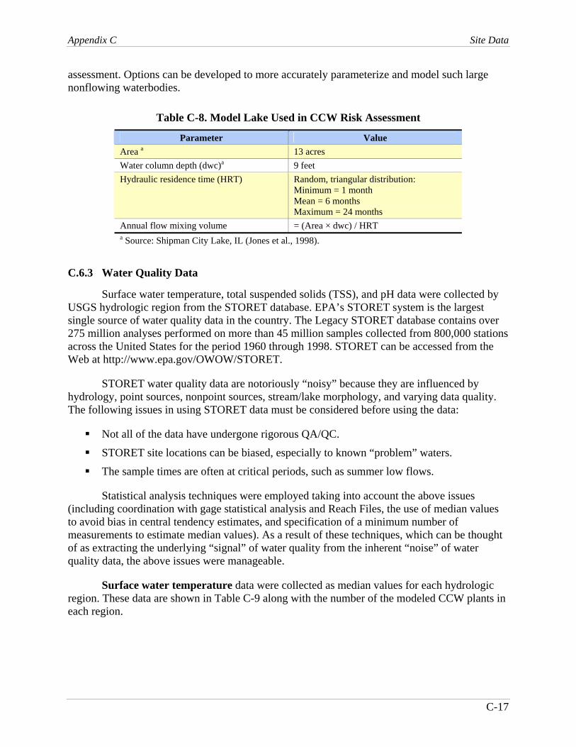
Appendix C Site Data
C-17
assessment. Options can be developed to more accurately parameterize and model such large nonflowing waterbodies.
Table C-8. Model Lake Used in CCW Risk Assessment
Parameter Value Area a 13 acres Water column depth (dwc)a 9 feet Hydraulic residence time (HRT) Random, triangular distribution:
Minimum = 1 month Mean = 6 months Maximum = 24 months
Annual flow mixing volume = (Area × dwc) / HRT a Source: Shipman City Lake, IL (Jones et al., 1998).
C.6.3 Water Quality Data
Surface water temperature, total suspended solids (TSS), and pH data were collected by USGS hydrologic region from the STORET database. EPA’s STORET system is the largest single source of water quality data in the country. The Legacy STORET database contains over 275 million analyses performed on more than 45 million samples collected from 800,000 stations across the United States for the period 1960 through 1998. STORET can be accessed from the Web at http://www.epa.gov/OWOW/STORET.
STORET water quality data are notoriously “noisy” because they are influenced by hydrology, point sources, nonpoint sources, stream/lake morphology, and varying data quality. The following issues in using STORET data must be considered before using the data:
Not all of the data have undergone rigorous QA/QC.
STORET site locations can be biased, especially to known “problem” waters.
The sample times are often at critical periods, such as summer low flows.
Statistical analysis techniques were employed taking into account the above issues (including coordination with gage statistical analysis and Reach Files, the use of median values to avoid bias in central tendency estimates, and specification of a minimum number of measurements to estimate median values). As a result of these techniques, which can be thought of as extracting the underlying “signal” of water quality from the inherent “noise” of water quality data, the above issues were manageable.
Surface water temperature data were collected as median values for each hydrologic region. These data are shown in Table C-9 along with the number of the modeled CCW plants in each region.

Appendix C Site Data
C-18
Table C-9. Regional Surface Water Temperatures: CCW Disposal Sites
Hydrologic Region
Surface Water Temperature (EC)
Number of CCW Plants
2 16 12 3 21 37 4 14 14 5 17 43 6 18 6 7 15 20 8 20 2 9 10 1
10 13 20 11 17 8 12 21 6 14 9 5 15 17 4 16 9 1 18 15 2
Data source: Legacy STORET database.
Total suspended solids data were collected separately for streams/rivers and lakes because lakes tend to have lower TSS levels. Annual median values were used to develop statistics. For rivers, the minimum, maximum, and geometric mean values were used to define log triangular distributions for each hydrologic region (Table C-10); these distributions were then sampled during the preparation of the source data files. (The geometric means were weighted by the annual number of measurements.) For lakes, data were limited and national statistics were developed, with the geometric mean of the median values being weighted by the number of measurements per year and the number of annual values in each region.
Table C-10. Surface Water Total Suspended Solids (TSS) Distributions
Annual Median TSS (log triangular distribution)
Hydrologic Region
Number of CCW Plants
No. of Measure-
ments
No. of Annual Medians Minimum Maximum
Weighted Geometric
Mean Geometric
Mean
1 0 9,007 33 3.2 40 8.0 6.0 2 12 47,202 38 10 316 32 40 3 37 43,395 36 6.3 79 25 25 4 14 29,577 37 6.3 794 25 25 5 43 39,900 38 4.0 100 25 25 6 6 4,137 28 5.0 316 16 20
(continued)

Appendix C Site Data
C-19
Table C-10. (continued) Annual Median TSS
(log triangular distribution)
Hydrologic Region
Number of CCW Plants
No. of Measure-
ments
No. of Annual Medians Minimum Maximum
Weighted Geometric
Mean Geometric
Mean
7 20 34,494 37 32 1,585 63 100 8 2 46,231 38 50 316 158 126 9 1 3,254 35 13 3,162 32 63
10 20 62,791 38 10 398 126 126 11 8 48,969 38 25 794 200 126 12 6 7,280 35 40 1,995 79 126 13 0 13,974 37 32 79,433 200 398 14 5 26,699 38 16 5,012 158 251 15 4 9,162 37 20 19,953 200 398 16 1 19,965 33 4 2,512 16 25 17 0 173,136 37 2 316 6.0 10 18 2 42,022 37 13 398 63 50
Lakes (national)
56 4,360 99 1 398 25 25
Data source: Legacy STORET database.
For surface water pH, the minimum, maximum, and weighted average annual median values were used to specify triangular distributions for each hydrologic region. Table C-11 provides these regional statistics, which were applied to both rivers and lakes.
To prepare the water quality data for the source datafile, the 181 CCW disposal sites were assigned to a hydrogeologic region using a GIS. For each region, 10,000-record TSS and pH data sets were created by sampling the distributions shown in Tables C-10 and C-11. During source data file preparation, TSS data were pulled from the appropriate regional data set sequentially for each iteration at a site.
Table C-11. Regional Surface Water pH Distributions
Annual Median pH (triangular distribution)
Hydrologic Region
Number of CCW Plants
No. of Measurements
No. of Annual Median Values Minimum Maximum
Weighted Average
Average Median pH
1 0 232,025 38 5.9 7.7 6.5 6.8 2 12 447,166 39 7.2 7.6 7.4 7.4 3 37 1,595,237 39 6.3 7.2 7.0 7.0 4 14 335,261 39 7.6 8.2 8.1 8.0 5 43 684,235 41 3.5 7.5 7.2 7.1 6 6 382,915 39 6.3 7.7 7.2 7.4
(continued)

Appendix C Site Data
C-20
Table C-11. (continued) Annual Median pH
(triangular distribution) Hydrologic
Region
Number of CCW Plants
No. of Measurements
No. of Annual Median Values Minimum Maximum
Weighted Average
Average Median pH
7 20 234,589 39 7.6 8.1 7.9 7.8 8 2 171,643 39 6.9 7.8 7.1 7.2 9 1 23,038 38 7.5 8.4 7.9 7.9
10 20 269,570 39 7.6 8.2 8.0 8.0 11 8 311,768 39 7.4 8.1 7.8 7.8 12 6 178,990 39 7.0 7.9 7.8 7.6 13 0 35,355 39 7.0 8.1 8.0 7.9 14 5 77,041 39 7.9 8.3 8.1 8.1 15 4 75,145 38 7.7 8.3 8.0 8.0 16 1 68,581 38 7.5 8.3 8.0 8.0 17 0 293,909 39 6.9 8.0 7.5 7.4 18 2 182,049 38 7.4 8.6 7.8 7.8
Data source: Legacy STORET database.
C.6.4 Distance to Surface Water
Because the CCW plant locations were not accurate in terms of locating the WMUs, a national empirical distribution of distances between the WMU and the nearest downgradient surface waterbodies (discussed in Appendix C, Section C.2.1) was developed using manual measurements on online maps and aerial photographs for a random selection of 30 CCW landfills and 29 CCW surface impoundments. Scaled USGS maps and aerial photographs were obtained from the Terraserver Web site (http://terraserver.usa.com/geographic.aspx) by entering each plant’s longitude and latitude. Labels on the maps, features on the photographs, and best professional judgment were used to identify the power plant and the surface impoundment or landfill in question, along with the nearest downgradient waterbody.
The nearest waterbody matching one of the following descriptions was used in the analysis:
Lakes or rivers beyond the facility boundary
Streams originating in or passing through the facility boundary and then coursing downstream beyond the property boundary
Streams with an order of 3 or greater (i.e., fishable waterbodies).
Stream order was determined by tracing the convergence of tributaries with order 1 assigned to the furthest upstream segment indicated on the map (both ephemeral and perennial streams were assigned as order 1). Topography on the map was used to determine if the waterbody was downgradient of the plant. Many CCW WMUs in the sample were located on a large waterbody.

Appendix C Site Data
C-21
Once the waterbody was identified, the scale provided on the maps and photos was used to measure the horizontal distance between the CCW impoundment or landfill and the waterbody. All assignments and measurements were independently checked for accuracy.
The two distributions (landfills and surface impoundments) were statistically compared using (1) a Wilcoxon Rank Sum Test (to determine whether one distribution is shifted to the right or left of the other distribution) and (2) a Quantile Test (to test for differences, that is, differing numbers of observations) between the two distributions for the values above a given percentile. The results of the Wilcoxon test showed a p value of 0.64, indicating no significant difference in the shape of the distributions. The Quantile Test evaluated every decile from 0.1 to 0.9, with adjustments to the lower percentiles to be estimated for large numbers of ties in the ranks for the lower end of the data. The nonsignificant p values ranged from 0.33 (for 90th percentile) to 0.17 (for the 40th percentile). One significant p value indicating differences between the two distributions occurred at the 17th percentile (p value = 0.066), but the remainder of the tests showed no significant differences. Based on these results, the distributions were judged to be similar and combined to produce the single distribution of 59 values used to produce a single empirical distribution (previously shown in Table C-2) that was applied nationally to both landfills and surface impoundments at the CCW sites.
C.5 References
Aller, L., T. Bennett, J.H. Lehr, R.J. Perry, and G. Hackett. 1987. DRASTIC: A Standardized System for Evaluating Pollution Potential Using Hydrogeologic Settings. EPA-600/2-87-035. U.S. Environmental Protection Agency. Office of Research and Development. Ada, OK. April.
Carsel, R.F., and R.S. Parrish. 1988. Developing joint probability distributions of soil water retention characteristics. Water Resources Research 24(5):755–769.
Carsel, R.F., R.S. Parrish, R.L. Jones, J.L. Hansen, and R.L. Lamb. 1988. Characterizing the uncertainty of pesticide leaching in agricultural soils. Journal of Contaminant Hydrology 2:111–124.
Clawges, R.M., and C.V. Price. 1999a. Digital Data Sets Describing Principal Aquifers, Surficial Geology, and Ground-Water Regions of the Conterminous United States. Open-File Report 99-77. U.S. Geological Survey, Rapid City, SD. Available: http://water.usgs.gov/pubs/ofr/ofr99-77/index.html.
Clawges, R.M., and C.V. Price. 1999b. Ground-water regions of the conterminous United States with unconsolidated watercourses. Edition: 1.0 (map). In Open-File Report 99-77. U.S. Geological Survey, Rapid City, SD. Data Retrieval: http://water.usgs.gov/lookup/getspatial?ofr99-77_gwreguw Metadata: http://water.usgs.gov/GIS/metadata/usgswrd/ofr99-77_gwreguw.html
Clawges, R.M., and C.V. Price. 1999c. Productive aquifers of the conterminous United States. Version 1.0 (map). In Open-File Report 99-77. U.S. Geological Survey, Rapid City, SD.

Appendix C Site Data
C-22
Data Retrieval: http://water.usgs.gov/lookup/getspatial?ofr99-77_aquif75m Metadata: http://water.usgs.gov/GIS/metadata/usgswrd/ofr99-77_aquif75m.html
Clawges, R.M., and C.V. Price. 1999d. Surficial geology of the conterminous United States. Version 1.0. In Open-File Report 99-77. U.S. Geological Survey, Rapid City, SD. Data Retrieval: http://water.usgs.gov/lookup/getspatial?ofr99-77_geol75m Metadata: http://water.usgs.gov/GIS/metadata/usgswrd/ofr99-77_geol75m.html
Heath, R.C. 1984. Ground-Water Regions of the United States. Water-Supply Paper 2242, U.S. Geological Survey, Washington, DC.
Heath, R.C. 1985. National Water Summary 1984. State Summaries of Groundwater Resources. Water-Supply Paper 2275. U.S. Geological Survey, Washington, DC.
Jones, R.D., S.W. Abel, W. Effland, R. Matzner, and R. Parker. 1998. An index reservoir for use in assessing drinking water exposures. Chapter IV in Proposed Methods for Basin-Scale Estimation of Pesticide Concentrations in Flowing Water and Reservoirs for Tolerance Reassessment, presented to the FIFRA Scientific Advisory Panel. July. http://www.epa.gov/oscpmont/sap/1998/july/1part4.pdf
Kocher, K., and R. Sartor. 1997. Derivation and use of data and table to determine stream flow values for water bodies. Memorandum to File, RTI Project 6720-005. Research Triangle Institute, Research Triangle Park, NC. June 16.
Miller, J.A. 1998. Principal Aquifers of the 48 Contiguous United States. Version 1.0. United States Geological Survey, Madison, WI. Metadata: http://www.atlas.usgs.gov/ aquifersm.html#Identification_Information
Miller, D.A., and R.A. White. 1998. A Conterminous United States Multi-Layer Soil Characteristics Data Set for Regional Climate and Hydrology Modeling. Available: http://www.essc.psu.edu/soil_info/index.cgi?soil_data&index.html
Newell, C.J., L.P. Hopkins, and P.B. Bedient. 1989. Hydrogeologic Database for Ground Water Modeling. API Publication No. 4476. American Petroleum Institute, Washington, DC.
Newell, C,J., L.P. Hopkins, and P.B. Bedient. 1990. A hydrogeologic database for ground water modeling. Ground Water 28(5):703–714.
Schwarz, G.E., and R.B. Alexander. 1995. State Soil Geographic (STATSGO) Data Base for the Conterminous United States. Edition: 1.1. Reston, VA. Available: http://water.usgs.gov/GIS/metadata/usgswrd/ussoils.html
USDA (U.S. Department of Agriculture). 1994. State Soil Geographic (STATSGO) Data Base. Data Use Information. Miscellaneous Publication No. 1492. Natural Resources Conservation Service, Fort Worth, TX. Available: http://www.ftw.nrcs.usda.gov/stat_data.html

Appendix C Site Data
C-23
U.S. EPA (Environmental Protection Agency). 1988. National Survey of Solid Waste (Municipal) Landfill Facilities (Draft). EPA/530-SW88-034. Office of Solid Waste and Emergency Response, Washington, DC. September.
U.S. EPA (Environmental Protection Agency). 1990. Office of Water Environmental and Program Information Systems Compendium. FY 1990. EPA 500/9-90-002. Office of Water, August.
U.S. EPA (Environmental Protection Agency). 1997. EPA’s Composite Model for Leachate Migration with Transformation Products (EPACMTP) User’s Guide. Office of Solid Waste, Washington, DC.
van der Leeden, F., F.L. Troise, and D.K. Todd. 1990. The Water Encyclopedia. 2nd Ed. Chelsea, MI: Lewis Publishers. 176 pp.

[This page intentionally left blank.]

Appendix C Attachment C-1: Soil Data
C-1-1
Attachment C-1: Soil Data
Plant Percent
Composition Megatexture
Code Average pH Average %
Organic MaterialA B Brown 43.9 SCL 6.0 1.2 A B Brown 51.1 SLT 6.5 1.6 A B Brown 5.0 SNL 6.9 1.4 A/C Power- Ace Operations 8.9 SCL 8.9 0.21 A/C Power- Ace Operations 32.0 SLT 8.4 0.46 A/C Power- Ace Operations 59.1 SNL 8.0 0.46 Allen 48.9 SCL 7.1 0.98 Allen 19.2 SLT 6.2 1.1 Allen 32.0 SNL 7.1 1.1 Alma 18.9 SCL 6.6 1.7 Alma 59.4 SLT 6.5 3.4 Alma 21.7 SNL 5.6 0.69 Antelope Valley 8.4 SCL 7.6 3.2 Antelope Valley 68.5 SLT 7.6 1.7 Antelope Valley 23.1 SNL 7.8 2.4 Arkwright 50.7 SCL 5.4 0.5 Arkwright 24.7 SLT 5.6 0.88 Arkwright 24.5 SNL 5.4 0.64 Asheville 6.3 SCL 5.4 0.43 Asheville 77.8 SLT 5.2 0.99 Asheville 15.8 SNL 5.4 1 Baldwin 39.5 SCL 6.2 1.3 Baldwin 58.6 SLT 6.0 1.6 Baldwin 1.9 SNL 6.5 1.4 Barry 35.8 SCL 4.8 3.6 Barry 23.5 SLT 4.8 7 Barry 40.7 SNL 4.8 4.4 Bay Front 11.7 SCL 7.3 4 Bay Front 21.1 SLT 7.1 3.8 Bay Front 67.2 SNL 7.1 1.4 Bay Shore 90.8 SCL 7.1 4.1 Bay Shore 4.3 SLT 7.2 2.6 Bay Shore 4.9 SNL 7.7 9.3 Belews Creek 69.2 SCL 5.2 0.34 Belews Creek 14.0 SLT 5.4 1
(continued)
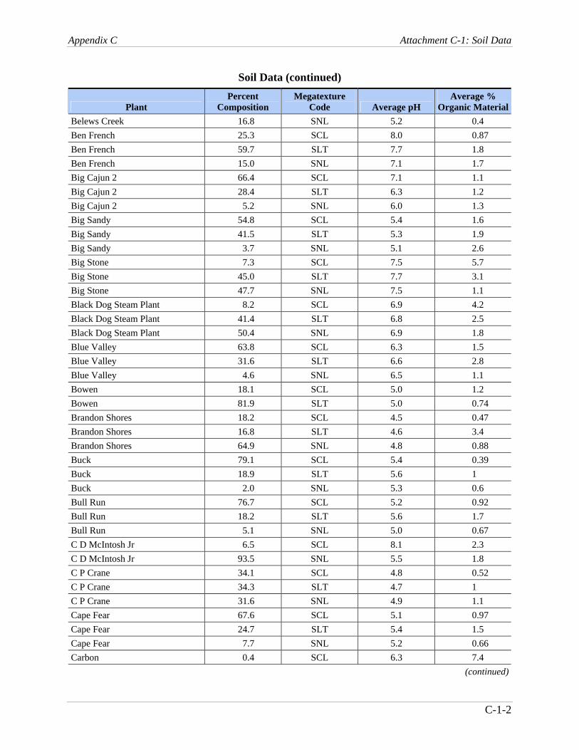
Appendix C Attachment C-1: Soil Data
C-1-2
Soil Data (continued)
Plant Percent
Composition Megatexture
Code Average pH Average %
Organic MaterialBelews Creek 16.8 SNL 5.2 0.4 Ben French 25.3 SCL 8.0 0.87 Ben French 59.7 SLT 7.7 1.8 Ben French 15.0 SNL 7.1 1.7 Big Cajun 2 66.4 SCL 7.1 1.1 Big Cajun 2 28.4 SLT 6.3 1.2 Big Cajun 2 5.2 SNL 6.0 1.3 Big Sandy 54.8 SCL 5.4 1.6 Big Sandy 41.5 SLT 5.3 1.9 Big Sandy 3.7 SNL 5.1 2.6 Big Stone 7.3 SCL 7.5 5.7 Big Stone 45.0 SLT 7.7 3.1 Big Stone 47.7 SNL 7.5 1.1 Black Dog Steam Plant 8.2 SCL 6.9 4.2 Black Dog Steam Plant 41.4 SLT 6.8 2.5 Black Dog Steam Plant 50.4 SNL 6.9 1.8 Blue Valley 63.8 SCL 6.3 1.5 Blue Valley 31.6 SLT 6.6 2.8 Blue Valley 4.6 SNL 6.5 1.1 Bowen 18.1 SCL 5.0 1.2 Bowen 81.9 SLT 5.0 0.74 Brandon Shores 18.2 SCL 4.5 0.47 Brandon Shores 16.8 SLT 4.6 3.4 Brandon Shores 64.9 SNL 4.8 0.88 Buck 79.1 SCL 5.4 0.39 Buck 18.9 SLT 5.6 1 Buck 2.0 SNL 5.3 0.6 Bull Run 76.7 SCL 5.2 0.92 Bull Run 18.2 SLT 5.6 1.7 Bull Run 5.1 SNL 5.0 0.67 C D McIntosh Jr 6.5 SCL 8.1 2.3 C D McIntosh Jr 93.5 SNL 5.5 1.8 C P Crane 34.1 SCL 4.8 0.52 C P Crane 34.3 SLT 4.7 1 C P Crane 31.6 SNL 4.9 1.1 Cape Fear 67.6 SCL 5.1 0.97 Cape Fear 24.7 SLT 5.4 1.5 Cape Fear 7.7 SNL 5.2 0.66 Carbon 0.4 SCL 6.3 7.4
(continued)

Appendix C Attachment C-1: Soil Data
C-1-3
Soil Data (continued)
Plant Percent
Composition Megatexture
Code Average pH Average %
Organic MaterialCarbon 95.8 SLT 7.8 3.4 Carbon 3.8 SNL 8.2 1.4 Cardinal 69.1 SCL 5.8 1 Cardinal 30.4 SLT 5.7 1.7 Cardinal 0.5 SNL 6.4 2 Cayuga 32.3 SCL 6.6 1.9 Cayuga 48.7 SLT 7.1 1.4 Cayuga 19.0 SNL 6.8 1.1 Chalk Point 6.9 SCL 4.6 0.58 Chalk Point 16.4 SLT 4.8 8.8 Chalk Point 76.7 SNL 4.6 1.1 Cholla 27.3 SCL 8.4 1.9 Cholla 61.0 SLT 8.1 0.62 Cholla 11.6 SNL 8.3 0.75 Cliffside 66.4 SCL 5.2 0.31 Cliffside 13.6 SLT 5.5 0.77 Cliffside 20.0 SNL 5.2 0.27 Clover 71.0 SCL 5.3 0.71 Clover 23.3 SLT 5.3 1.3 Clover 5.7 SNL 5.1 0.65 Coal Creek 6.1 SCL 6.8 3 Coal Creek 82.7 SLT 7.6 1.7 Coal Creek 11.2 SNL 8.2 2.8 Coleto Creek 12.1 SCL 7.0 1.1 Coleto Creek 86.0 SLT 7.4 0.78 Coleto Creek 1.8 SNL 6.2 0.75 Colstrip 9.0 SCL 8.0 0.79 Colstrip 63.0 SLT 8.2 0.73 Colstrip 27.9 SNL 8.3 0.54 Conemaugh 11.8 SCL 5.0 2.7 Conemaugh 81.4 SLT 4.8 1.3 Conemaugh 6.8 SNL 4.5 1.8 Conesville 44.0 SCL 5.4 2.2 Conesville 45.5 SLT 5.6 1.9 Conesville 10.5 SNL 5.0 2.2 Council Bluffs 43.3 SCL 7.5 1.5 Council Bluffs 47.2 SLT 7.6 1.2 Council Bluffs 9.6 SNL 7.7 0.74 Crawford 48.4 SCL 6.8 1.9
(continued)

Appendix C Attachment C-1: Soil Data
C-1-4
Soil Data (continued)
Plant Percent
Composition Megatexture
Code Average pH Average %
Organic MaterialCrawford 23.6 SLT 6.7 1.4 Crawford 28.0 SNL 6.7 0.82 Crist 18.8 SCL 5.4 4.5 Crist 32.3 SLT 5.3 1.1 Crist 48.8 SNL 5.4 3.3 Cross 3.0 SCL 5.0 1.3 Cross 46.0 SLT 4.6 0.58 Cross 51.0 SNL 4.9 1.2 Cumberland 61.1 SCL 5.3 1.6 Cumberland 34.2 SLT 5.7 0.98 Cumberland 4.8 SNL 5.2 1.3 Dale 91.7 SCL 6.4 1.9 Dale 8.2 SLT 6.4 2 Dale 0.1 SNL 6.7 1.3 Dallman 66.2 SCL 6.4 1.8 Dallman 33.3 SLT 6.7 1.2 Dallman 0.5 SNL 7.0 1.1 Dan E Karn 0.01 SCL 7.0 3 Dan E Karn 53.6 SLT 7.9 4.2 Dan E Karn 46.3 SNL 7.8 5.4 Dan River 73.3 SCL 5.0 0.39 Dan River 12.0 SLT 5.3 1.4 Dan River 14.7 SNL 5.1 0.6 Danskammer 89.8 SLT 5.8 2.9 Danskammer 10.2 SNL 6.9 2.8 Dave Johnston 2.2 SCL 8.9 0.96 Dave Johnston 36.6 SLT 8.2 1.2 Dave Johnston 61.2 SNL 8.2 1.1 Dickerson 6.1 SCL 5.1 0.52 Dickerson 93.9 SLT 5.2 0.68 Dolet Hills 65.7 SCL 4.8 0.97 Dolet Hills 21.6 SLT 5.0 0.77 Dolet Hills 12.7 SNL 5.1 1.1 Duck Creek 65.5 SCL 6.4 0.82 Duck Creek 33.6 SLT 6.5 0.6 Duck Creek 0.9 SNL 7.0 0.98 Dunkirk 8.8 SCL 7.3 5.4 Dunkirk 79.6 SLT 6.9 4.6 Dunkirk 11.6 SNL 6.5 2.7
(continued)

Appendix C Attachment C-1: Soil Data
C-1-5
Soil Data (continued)
Plant Percent
Composition Megatexture
Code Average pH Average %
Organic MaterialE D Edwards 49.5 SCL 6.4 1.1 E D Edwards 29.8 SLT 6.3 1.2 E D Edwards 20.6 SNL 6.8 1.1 E W Brown 92.9 SCL 6.4 3.7 E W Brown 7.1 SLT 6.6 3.8 Eckert Station 4.8 SCL 7.2 4.5 Eckert Station 82.0 SLT 6.9 1.2 Eckert Station 13.2 SNL 6.7 0.5 Edgewater 58.5 SCL 7.3 3.3 Edgewater 3.7 SLT 7.3 1.2 Edgewater 37.8 SNL 6.8 2.2 Elmer W Stout 29.9 SCL 6.7 1.9 Elmer W Stout 56.7 SLT 7.0 1.2 Elmer W Stout 13.3 SNL 6.8 0.8 F B Culley 45.3 SCL 5.9 0.93 F B Culley 48.9 SLT 6.5 2 F B Culley 5.8 SNL 6.9 1.1 Fayette Power Prj 51.9 SCL 7.7 3.8 Fayette Power Prj 35.7 SLT 7.6 1.2 Fayette Power Prj 12.5 SNL 7.1 1 Flint Creek 62.2 SCL 4.9 0.87 Flint Creek 37.8 SLT 5.3 0.69 Fort Martin 45.9 SCL 5.6 1.2 Fort Martin 54.1 SLT 5.2 1.9 Fort Martin 0.04 SNL 4.6 2.5 Frank E Ratts 30.9 SCL 5.8 1.5 Frank E Ratts 58.0 SLT 6.3 1.1 Frank E Ratts 11.1 SNL 7.0 0.73 G G Allen 85.9 SCL 5.3 0.36 G G Allen 11.9 SLT 5.6 1.1 G G Allen 2.2 SNL 5.2 0.28 Gadsden 45.2 SCL 4.8 0.68 Gadsden 46.4 SLT 5.3 1.3 Gadsden 8.5 SNL 5.1 0.97 Gallatin 56.1 SCL 5.6 0.94 Gallatin 43.9 SLT 5.4 0.94 Gen J M Gavin 35.9 SCL 6.0 1.4 Gen J M Gavin 46.1 SLT 5.6 2.1 Gen J M Gavin 18.0 SNL 5.1 1.3
(continued)

Appendix C Attachment C-1: Soil Data
C-1-6
Soil Data (continued)
Plant Percent
Composition Megatexture
Code Average pH Average %
Organic MaterialGenoa 14.3 SCL 6.1 2.3 Genoa 64.6 SLT 6.6 1.8 Genoa 21.0 SNL 6.1 0.97 Gibson 55.3 SCL 6.6 1.5 Gibson 43.2 SLT 6.4 1.1 Gibson 1.5 SNL 7.3 0.67 Gorgas 17.0 SCL 4.6 0.42 Gorgas 53.0 SLT 5.1 0.77 Gorgas 30.0 SNL 5.2 0.73 Green River 48.4 SCL 5.9 1 Green River 51.6 SLT 6.0 1.4 Greene County 19.5 SCL 5.1 1.8 Greene County 72.6 SLT 5.2 1.4 Greene County 7.9 SNL 4.9 1.6 H B Robinson 0.1 SCL 5.2 0.75 H B Robinson 32.6 SLT 4.8 1 H B Robinson 67.3 SNL 5.3 0.6 Hammond 54.7 SCL 5.1 0.74 Hammond 33.8 SLT 5.3 1.3 Hammond 11.5 SNL 5.0 0.75 Harllee Branch 54.7 SCL 5.3 0.49 Harllee Branch 15.3 SLT 5.6 0.97 Harllee Branch 30.0 SNL 5.3 0.47 Harrison 48.8 SCL 5.6 1 Harrison 51.2 SLT 5.0 2.1 Hatfield's Ferry 39.3 SCL 5.7 1.8 Hatfield's Ferry 60.4 SLT 5.3 1.6 Hatfield's Ferry 0.3 SNL 4.6 2.5 Hennepin 44.6 SCL 6.4 1.5 Hennepin 38.2 SLT 6.7 1.1 Hennepin 17.2 SNL 7.0 1.3 Heskett 39.9 SCL 8.0 2.1 Heskett 44.1 SLT 7.6 2.4 Heskett 16.0 SNL 7.7 1.9 Holcomb 4.4 SLT 7.9 0.67 Holcomb 95.6 SNL 7.3 0.75 Homer City 11.0 SCL 4.9 2.9 Homer City 84.5 SLT 4.8 1.6 Homer City 4.5 SNL 4.5 2.1
(continued)

Appendix C Attachment C-1: Soil Data
C-1-7
Soil Data (continued)
Plant Percent
Composition Megatexture
Code Average pH Average %
Organic MaterialHoot Lake 3.1 SCL 7.5 5.4 Hoot Lake 38.9 SLT 7.7 2.6 Hoot Lake 58.1 SNL 7.5 1.3 Hugo 55.1 SCL 6.6 1.4 Hugo 35.8 SLT 6.7 1.6 Hugo 9.2 SNL 5.3 0.7 Hunter 90.8 SCL 8.3 0.73 Hunter 3.5 SLT 8.2 2 Hunter 5.7 SNL 8.5 0.75 Huntington 4.5 SCL 8.6 1.5 Huntington 79.5 SLT 8.0 2.4 Huntington 15.9 SNL 8.6 1.3 Intermountain 46.9 SCL 8.6 0.7 Intermountain 8.3 SLT 8.9 0.51 Intermountain 44.8 SNL 8.8 0.44 J H Campbell 5.0 SLT 7.1 1.8 J H Campbell 95.0 SNL 5.9 1.2 J M Stuart 73.5 SCL 6.5 1.6 J M Stuart 24.8 SLT 6.8 2.4 J M Stuart 1.7 SNL 5.5 2 J R Whiting 80.6 SCL 7.1 4.2 J R Whiting 17.1 SLT 7.1 2.1 J R Whiting 2.3 SNL 6.8 2.8 Jack McDonough 58.9 SCL 5.2 0.46 Jack McDonough 7.8 SLT 5.6 1.1 Jack McDonough 33.3 SNL 5.3 0.37 Jack Watson 20.5 SCL 6.7 11 Jack Watson 46.8 SLT 4.8 3 Jack Watson 32.8 SNL 4.9 3.8 James H Miller Jr 17.0 SCL 4.6 0.42 James H Miller Jr 53.0 SLT 5.1 0.77 James H Miller Jr 30.0 SNL 5.2 0.73 Jim Bridger 1.4 SCL 8.7 0.75 Jim Bridger 37.9 SLT 8.6 0.52 Jim Bridger 60.6 SNL 8.2 0.64 John E Amos 35.8 SCL 6.3 1.6 John E Amos 64.2 SLT 5.1 2.2 John Sevier 43.2 SCL 6.2 1.6 John Sevier 56.7 SLT 5.8 1.2
(continued)

Appendix C Attachment C-1: Soil Data
C-1-8
Soil Data (continued)
Plant Percent
Composition Megatexture
Code Average pH Average %
Organic MaterialJohn Sevier 0.2 SNL 5.0 0.67 Johnsonville 39.2 SCL 5.1 1.7 Johnsonville 57.3 SLT 5.2 1.3 Johnsonville 3.5 SNL 4.7 1.5 Joliet 29 52.8 SCL 7.1 2.7 Joliet 29 43.5 SLT 7.0 2.1 Joliet 29 3.7 SNL 7.1 1.8 Keystone 7.7 SCL 4.9 2.8 Keystone 90.1 SLT 4.9 1.4 Keystone 2.2 SNL 4.5 2.2 Killen Station 74.3 SCL 6.0 1.9 Killen Station 24.0 SLT 6.3 2.2 Killen Station 1.8 SNL 6.2 1.7 Kingston 66.7 SCL 5.0 1.2 Kingston 21.0 SLT 5.5 1.7 Kingston 12.3 SNL 5.0 0.67 Kraft 57.1 SCL 7.2 11 Kraft 22.8 SLT 5.0 1.3 Kraft 20.1 SNL 5.0 1.4 L V Sutton 18.0 SCL 6.1 3.9 L V Sutton 32.4 SLT 5.0 3.7 L V Sutton 49.6 SNL 5.0 1.6 Lansing 9.0 SCL 5.8 2.6 Lansing 67.7 SLT 6.8 2.1 Lansing 23.3 SNL 6.2 1.4 Laramie R Station 41.1 SLT 8.1 0.87 Laramie R Station 58.9 SNL 7.9 1.2 Lawrence EC 51.5 SCL 6.6 1.9 Lawrence EC 47.7 SLT 6.8 2.9 Lawrence EC 0.8 SNL 7.5 0.75 Lee 16.4 SCL 5.0 1.3 Lee 51.1 SLT 5.0 1.3 Lee 32.5 SNL 5.1 0.96 Leland Olds 13.5 SCL 7.8 2.6 Leland Olds 52.9 SLT 7.6 1.9 Leland Olds 33.6 SNL 7.5 2 Lon Wright 25.7 SCL 7.5 1.5 Lon Wright 8.4 SLT 7.0 2.1 Lon Wright 65.9 SNL 7.8 1.4
(continued)
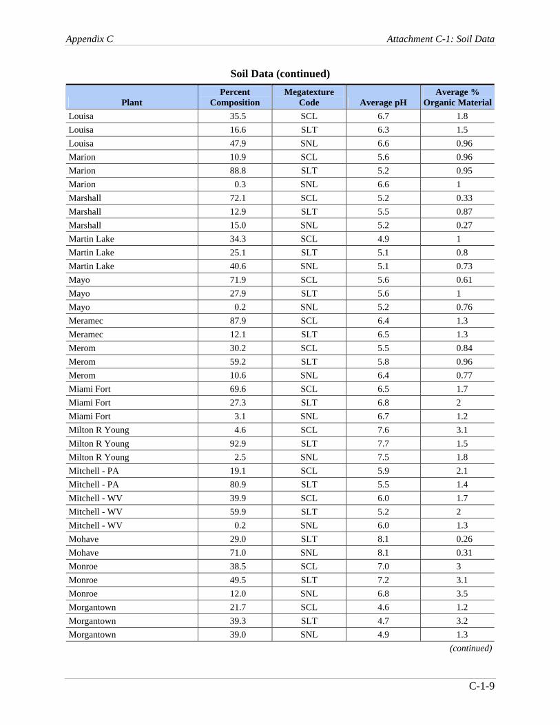
Appendix C Attachment C-1: Soil Data
C-1-9
Soil Data (continued)
Plant Percent
Composition Megatexture
Code Average pH Average %
Organic MaterialLouisa 35.5 SCL 6.7 1.8 Louisa 16.6 SLT 6.3 1.5 Louisa 47.9 SNL 6.6 0.96 Marion 10.9 SCL 5.6 0.96 Marion 88.8 SLT 5.2 0.95 Marion 0.3 SNL 6.6 1 Marshall 72.1 SCL 5.2 0.33 Marshall 12.9 SLT 5.5 0.87 Marshall 15.0 SNL 5.2 0.27 Martin Lake 34.3 SCL 4.9 1 Martin Lake 25.1 SLT 5.1 0.8 Martin Lake 40.6 SNL 5.1 0.73 Mayo 71.9 SCL 5.6 0.61 Mayo 27.9 SLT 5.6 1 Mayo 0.2 SNL 5.2 0.76 Meramec 87.9 SCL 6.4 1.3 Meramec 12.1 SLT 6.5 1.3 Merom 30.2 SCL 5.5 0.84 Merom 59.2 SLT 5.8 0.96 Merom 10.6 SNL 6.4 0.77 Miami Fort 69.6 SCL 6.5 1.7 Miami Fort 27.3 SLT 6.8 2 Miami Fort 3.1 SNL 6.7 1.2 Milton R Young 4.6 SCL 7.6 3.1 Milton R Young 92.9 SLT 7.7 1.5 Milton R Young 2.5 SNL 7.5 1.8 Mitchell - PA 19.1 SCL 5.9 2.1 Mitchell - PA 80.9 SLT 5.5 1.4 Mitchell - WV 39.9 SCL 6.0 1.7 Mitchell - WV 59.9 SLT 5.2 2 Mitchell - WV 0.2 SNL 6.0 1.3 Mohave 29.0 SLT 8.1 0.26 Mohave 71.0 SNL 8.1 0.31 Monroe 38.5 SCL 7.0 3 Monroe 49.5 SLT 7.2 3.1 Monroe 12.0 SNL 6.8 3.5 Morgantown 21.7 SCL 4.6 1.2 Morgantown 39.3 SLT 4.7 3.2 Morgantown 39.0 SNL 4.9 1.3
(continued)

Appendix C Attachment C-1: Soil Data
C-1-10
Soil Data (continued)
Plant Percent
Composition Megatexture
Code Average pH Average %
Organic MaterialMountaineer (1301) 56.1 SCL 6.0 1.6 Mountaineer (1301) 34.2 SLT 5.9 2.2 Mountaineer (1301) 9.8 SNL 4.9 2.5 Mt Storm 4.1 SCL 5.0 2.9 Mt Storm 65.3 SLT 4.7 1.4 Mt Storm 30.6 SNL 4.4 1 Muscatine Plant #1 46.8 SCL 6.6 1.8 Muscatine Plant #1 27.4 SLT 6.4 1.4 Muscatine Plant #1 25.8 SNL 6.6 0.84 Muskogee 30.9 SCL 6.5 1.7 Muskogee 53.1 SLT 6.8 1.1 Muskogee 16.0 SNL 6.7 1 Neal North 36.7 SCL 7.9 1.1 Neal North 46.5 SLT 7.9 0.67 Neal North 16.9 SNL 7.7 0.73 Neal South 34.0 SCL 7.8 1.1 Neal South 50.7 SLT 7.8 0.69 Neal South 15.3 SNL 7.7 0.73 Nebraska City 55.5 SCL 7.4 1.4 Nebraska City 35.5 SLT 7.3 1.7 Nebraska City 9.0 SNL 7.7 0.74 New Castle 5.1 SCL 7.7 0.73 New Castle 81.6 SLT 5.9 2.8 New Castle 13.2 SNL 6.1 1.5 Newton 37.9 SCL 5.5 0.54 Newton 61.3 SLT 5.5 0.53 Newton 0.7 SNL 6.5 0.85 North Omaha 29.0 SCL 7.4 1.5 North Omaha 60.1 SLT 7.7 0.82 North Omaha 11.0 SNL 7.7 0.74 Northeastern 76.9 SCL 6.7 2.1 Northeastern 21.3 SLT 6.3 2.2 Northeastern 1.8 SNL 5.6 2 Nucla 61.2 SLT 7.9 0.98 Nucla 38.8 SNL 8.1 0.55 Oklaunion 92.2 SCL 8.0 1.7 Oklaunion 7.0 SLT 7.9 0.94 Oklaunion 0.7 SNL 7.3 1.5 Paradise 14.8 SCL 5.6 1.4
(continued)

Appendix C Attachment C-1: Soil Data
C-1-11
Soil Data (continued)
Plant Percent
Composition Megatexture
Code Average pH Average %
Organic MaterialParadise 85.2 SLT 5.9 1.2 Petersburg 29.7 SCL 5.9 1.5 Petersburg 62.9 SLT 6.3 1.2 Petersburg 7.5 SNL 7.2 0.59 Pleasant Prairie 97.2 SCL 7.1 1.7 Pleasant Prairie 2.8 SNL 7.3 1.5 Port Washington 86.3 SCL 7.3 3.3 Port Washington 7.7 SLT 7.5 0.68 Port Washington 6.1 SNL 7.3 3 Portland 8.7 SCL 5.8 0.58 Portland 90.8 SLT 5.5 1.1 Portland 0.5 SNL 6.0 1.8 Possum Point 6.3 SCL 4.6 0.58 Possum Point 43.0 SLT 4.9 3 Possum Point 50.7 SNL 4.9 0.8 Potomac River 13.3 SCL 4.5 0.56 Potomac River 35.5 SLT 4.9 2.8 Potomac River 51.2 SNL 5.0 1.1 Presque Isle 18.7 SLT 5.2 2.5 Presque Isle 81.3 SNL 5.3 3.1 R Gallagher 40.4 SCL 5.6 1.5 R Gallagher 59.0 SLT 5.9 2.1 R Gallagher 0.5 SNL 6.9 1.4 R M Schahfer 2.1 SCL 7.1 3.8 R M Schahfer 6.5 SLT 6.9 2.9 R M Schahfer 91.4 SNL 6.6 1.5 Reid Gardner 13.3 SCL 8.4 0.29 Reid Gardner 21.6 SLT 8.3 0.58 Reid Gardner 65.1 SNL 8.4 0.34 Richard Gorsuch 69.9 SCL 6.1 1.7 Richard Gorsuch 27.0 SLT 5.9 2.4 Richard Gorsuch 3.0 SNL 5.1 2.6 Riverbend 77.4 SCL 5.3 0.37 Riverbend 20.1 SLT 5.7 1.1 Riverbend 2.5 SNL 5.2 0.45 Rodemacher 42.9 SCL 6.5 0.96 Rodemacher 51.4 SLT 6.5 0.92 Rodemacher 5.7 SNL 5.3 0.85 Roxboro 40.3 SCL 5.5 0.47
(continued)

Appendix C Attachment C-1: Soil Data
C-1-12
Soil Data (continued)
Plant Percent
Composition Megatexture
Code Average pH Average %
Organic MaterialRoxboro 55.7 SLT 6.0 0.79 Roxboro 4.0 SNL 5.5 1.4 Sandow 0.8 SCL 6.9 0.5 Sandow 37.4 SLT 6.3 0.66 Sandow 61.8 SNL 6.3 0.64 Scherer 58.5 SCL 5.3 0.39 Scherer 12.8 SLT 5.5 0.97 Scherer 28.7 SNL 5.3 0.42 Shawnee 9.5 SCL 5.8 1 Shawnee 84.2 SLT 5.6 1.4 Shawnee 6.3 SNL 6.5 1.1 Shawville 5.2 SCL 5.0 3 Shawville 82.6 SLT 4.9 1.1 Shawville 12.2 SNL 4.4 1.2 Sheldon 62.7 SCL 6.8 2.3 Sheldon 33.2 SLT 7.0 1.6 Sheldon 4.1 SNL 6.9 2 South Oak Creek 95.5 SCL 7.1 1.9 South Oak Creek 4.5 SNL 7.3 1.6 Springerville 10.0 SLT 8.1 0.79 Springerville 90.0 SNL 7.9 0.79 St Johns River Power 27.1 SCL 6.9 49 St Johns River Power 0.4 SLT 5.0 1.3 St Johns River Power 72.5 SNL 5.2 1.1 Stanton Energy Ctr 0.8 SCL 7.0 10 Stanton Energy Ctr 2.4 SLT 7.7 1 Stanton Energy Ctr 96.8 SNL 5.3 4.8 Stockton Cogen Company 89.9 SCL 7.6 1.8 Stockton Cogen Company 6.6 SLT 7.5 1.5 Stockton Cogen Company 3.5 SNL 6.8 0.51 Syl Laskin 8.5 SCL 6.5 3.2 Syl Laskin 4.6 SLT 6.3 6.3 Syl Laskin 86.9 SNL 5.8 3.1 Tecumseh EC 55.2 SCL 6.6 2 Tecumseh EC 41.9 SLT 6.9 2.6 Tecumseh EC 2.9 SNL 7.6 0.62 Texas-New Mexico 4.4 SCL 7.0 0.61 Texas-New Mexico 43.5 SLT 6.3 0.67 Texas-New Mexico 52.1 SNL 6.0 0.77
(continued)

Appendix C Attachment C-1: Soil Data
C-1-13
Soil Data (continued)
Plant Percent
Composition Megatexture
Code Average pH Average %
Organic MaterialTitus 31.8 SCL 6.0 0.76 Titus 63.6 SLT 5.6 1.4 Titus 4.6 SNL 5.0 0.98 Trimble County 57.3 SCL 6.3 2 Trimble County 41.9 SLT 6.5 1.9 Trimble County 0.8 SNL 5.9 1.7 Tyrone 92.1 SCL 6.3 3.7 Tyrone 7.9 SLT 6.6 3.9 Valley 98.5 SCL 6.9 1.2 Valley 0.2 SLT 7.5 0.45 Valley 1.3 SNL 7.4 1.3 Vermilion 82.5 SCL 6.9 1.3 Vermilion 16.6 SLT 7.0 1.2 Vermilion 0.8 SNL 7.2 1.1 Victor J Daniel Jr 46.2 SCL 4.6 2.2 Victor J Daniel Jr 27.7 SLT 4.7 2.3 Victor J Daniel Jr 26.1 SNL 4.7 16 W A Parish 95.8 SCL 7.4 1.4 W A Parish 4.2 SLT 7.9 0.74 W H Weatherspoon 7.4 SCL 5.5 1.9 W H Weatherspoon 50.4 SLT 4.7 2.2 W H Weatherspoon 42.2 SNL 4.8 1.3 W S Lee 68.0 SCL 5.3 0.48 W S Lee 9.0 SLT 5.7 1 W S Lee 23.0 SNL 5.3 0.41 Wabash River 22.0 SCL 6.4 1.6 Wabash River 48.5 SLT 6.9 1.2 Wabash River 29.5 SNL 6.7 1.2 Walter C Beckjord 71.6 SCL 6.3 1.4 Walter C Beckjord 26.5 SLT 6.7 2 Walter C Beckjord 1.9 SNL 6.6 1.1 Wansley 46.3 SCL 5.2 0.52 Wansley 18.1 SLT 5.6 1.2 Wansley 35.5 SNL 5.4 0.5 Warrick 45.8 SCL 6.0 0.95 Warrick 48.6 SLT 6.5 1.9 Warrick 5.6 SNL 7.0 1.1 Waukegan 43.9 SCL 6.6 1 Waukegan 18.1 SLT 6.6 1.4
(continued)

Appendix C Attachment C-1: Soil Data
C-1-14
Soil Data (continued)
Plant Percent
Composition Megatexture
Code Average pH Average %
Organic MaterialWaukegan 38.0 SNL 6.7 0.8 Weston 33.5 SLT 5.6 1.7 Weston 66.5 SNL 6.0 1.4 Widows Creek 64.5 SCL 5.3 0.88 Widows Creek 20.0 SLT 5.2 1.4 Widows Creek 15.5 SNL 5.4 1.2 Will County 40.0 SCL 6.8 1.8 Will County 52.7 SLT 7.0 0.96 Will County 7.2 SNL 7.1 0.98 Wyodak 1.3 SCL 8.1 0.38 Wyodak 40.2 SLT 7.9 1.1 Wyodak 58.5 SNL 7.9 0.93 Yates 47.8 SCL 5.2 0.48 Yates 17.7 SLT 5.6 1.2 Yates 34.5 SNL 5.3 0.48

Appendix C
Attachm
ent C-2: H
ydrogeologic Environment
C
-2-1
Attachment C-2: Hydrogeologic Environment Hydrogeologic Setting Hydrogeologic Environment
Plant Code Description Code Description Percentage Comment
Big Cajun 2 10Ba River Alluvium With Overbank Deposits
6 River Valleys and Floodplains with Overbank Deposit
100 Predominant alluvial setting (100% alluvium); soils have significant fines (SCL+SLT = 95%)
A B Brown 6Fa River Alluvium With Overbank Deposits
6 River Valleys and Floodplains with Overbank Deposit
100 Predominant alluvial setting; soils have significant fines (SCL+SLT = 95%)
A/C Power- Ace Operations
2C Alluvial Fans 5 Alluvial Basins Valleys and Fans
100 Based on surficial geology; consistent with alluvial fan setting
Allen 10Ba River Alluvium With Overbank Deposits
6 River Valleys and Floodplains with Overbank Deposit
100 Setting based on aquifer coverages, surficial geology; Heath (1985) and soils indicate overbank deposits
Alma 7Ea River Alluvium With Overbank Deposits
6 River Valleys and Floodplains with Overbank Deposit
50 Percentage based on SNL/SCL soils; setting based on productive aquifers and surficial geology
Alma 7Eb River Alluvium Without Overbank Deposits
7 River Valleys and Floodplains without Overbank Deposits
50 Percentage based on SNL/SCL soils; setting based on productive aquifers and surficial geology
Antelope Valley 7G Thin Till Over Bedded Sedimentary Rock
3 Till Over Sedimentary Rock 100 Based on principal aquifer and surficial geology coverages
Arkwright 8D Regolith 1 Metamorphic and Igneous 100 Most common Piedmont setting (residuum) Asheville 8B Alluvial Mountain Valleys 5 Alluvial Basins Valleys and
Fans 100 Appropriate for alluvial blue ridge valley
(colluvium) Baldwin 7Ea River Alluvium With
Overbank Deposits 6 River Valleys and Floodplains
with Overbank Deposit 70 Percentage based on surficial geology (74%
Floodplain and alluvium gravel terraces) Baldwin 7G Thin Till Over Bedded
Sedimentary Rock 3 Till Over Sedimentary Rock 30 Percentage based on surficial geology (74%
Floodplain and alluvium gravel terraces) (continued)

Appendix C
Attachm
ent C-2: H
ydrogeologic Environment
C
-2-2
Hydrogeologic Environment (continued) Hydrogeologic Setting Hydrogeologic Environment
Plant Code Description Code Description Percentage Comment
Barry 10Ba River Alluvium With Overbank Deposits
6 River Valleys and Floodplains with Overbank Deposit
100 Predominant alluvial setting, significant fine grained soils = overbank deposits
Bay Front 7Bb Outwash Over Bedded Sedimentary Rock
2 Bedded Sedimentary Rock 70 Percentage based on productive aquifers
Bay Front 7D Buried Valley 4 Sand and Gravel 30 Percentage based on productive aquifers Bay Shore 7Ac Glacial Till Over Solution
Limestone 12 Solution Limestone 100 Closest setting considering carbonate
aquifers, high SCL soils, and lake deposits surficial geology
Belews Creek 6H Triassic Basins 2 Bedded Sedimentary Rock 50 Sources somewhat dissimilar; fraction based on surficial geology; Triassic basin
Belews Creek 8D Regolith 1 Metamorphic and Igneous 50 Sources somewhat dissimilar; fraction based on surficial geology
Ben French 6Da Alternating Sandstone, Limestone and Shale - Thin Soil
2 Bedded Sedimentary Rock 60 Percentage, thin soils based on surficial geology
Ben French 6Fa River Alluvium With Overbank Deposits
6 River Valleys and Floodplains with Overbank Deposit
40 Percentage based on surficial geology; significant fine soils (25% SCL)
Big Sandy 6Da Alternating Sandstone, Limestone and Shale - Thin Soil
2 Bedded Sedimentary Rock 50 Percentage based on surficial geology; thin soils inferred from colluvium
Big Sandy 6Fa River Alluvium With Overbank Deposits
6 River Valleys and Floodplains with Overbank Deposit
50 Percentage based on surficial geology; soils have significant fines (SCL+SLT = 95%)
Big Stone 7Ba Outwash 8 Outwash 100 Based on surficial geology Black Dog Steam Plant
7Bb Outwash Over Bedded Sedimentary Rock
2 Bedded Sedimentary Rock 100 Based on surficial geology, aquifer coverages
Blue Valley 7Aa Glacial Till Over Bedded Sedimentary Rock
3 Till Over Sedimentary Rock 80 Percentage based on Heath (1985), productive aquifers
(continued)

Appendix C
Attachm
ent C-2: H
ydrogeologic Environment
C
-2-3
Hydrogeologic Environment (continued) Hydrogeologic Setting Hydrogeologic Environment
Plant Code Description Code Description Percentage Comment
Blue Valley 7Ea River Alluvium With Overbank Deposits
6 River Valleys and Floodplains with Overbank Deposit
20 Percentage based on Heath (1985), productive aquifers
Bowen 6Db Alternating Sandstone, Limestone and Shale - Deep Regolith
2 Bedded Sedimentary Rock 100 Based on aquifers, surficial residuum (massive red clay); metamorphic surficial geology not consistent with Valley and Ridge
Brandon Shores 10Ab Unconsolidated and Semi-Consolidated Shallow Surficial Aquifer
10 Unconsolidated and Semiconsolidated Shallow Aquifers
100 Assigned based on location and aquifer and surficial geology coverages; Heath region incorrect (it's Atlantic Coastal Plain, not Piedmont)
Buck 8E River Alluvium 6 River Valleys and Floodplains with Overbank Deposit
100 Based on productive aquifer & Heath region coverages
Bull Run 6Db Alternating Sandstone, Limestone and Shale - Deep Regolith
2 Bedded Sedimentary Rock 60 Percentage based on surficial geology
Bull Run 6Fa River Alluvium With Overbank Deposits
6 River Valleys and Floodplains with Overbank Deposit
40 Percentage based on surficial geology; high SCL (77%) = overbank deposits
C D McIntosh Jr
11A Solution Limestone and Shallow Surficial Aquifers
12 Solution Limestone 100 Based on both aquifer coverages
C P Crane 10Aa Regional Aquifers 4 Sand and Gravel 50 Appears to be on border between Piedmont and Coastal Plain
C P Crane 8D Regolith 1 Metamorphic and Igneous 50 Appears to be on border between Piedmont and Coastal Plain
Cape Fear 6H Triassic Basins 2 Bedded Sedimentary Rock 20 Percentage based on productive aquifer & Heath region coverages; Triassic basin
Cape Fear 8E River Alluvium 6 River Valleys and Floodplains with Overbank Deposit
80 Percentage based on productive aquifer & Heath region coverages
Carbon 4B Consolidated Sedimentary Rock
2 Bedded Sedimentary Rock 100 Setting based on aquifer and surficial geology coverages
(continued)

Appendix C
Attachm
ent C-2: H
ydrogeologic Environment
C
-2-4
Hydrogeologic Environment (continued) Hydrogeologic Setting Hydrogeologic Environment
Plant Code Description Code Description Percentage Comment
Cardinal 6Da Alternating Sandstone, Limestone and Shale - Thin Soil
2 Bedded Sedimentary Rock 30 Percentage based on surficial geology; soils with low (<1%) SNL
Cardinal 6Fa River Alluvium With Overbank Deposits
6 River Valleys and Floodplains with Overbank Deposit
70 Percentage based on surficial geology; soils with low (<1%) SNL
Cayuga 7D Buried Valley 4 Sand and Gravel 100 Glaciofluvial aquifer overlaid by alluvial deposits
Chalk Point 10Ab Unconsolidated and Semi-Consolidated Shallow Surficial Aquifer
10 Unconsolidated and Semiconsolidated Shallow Aquifers
100 Predominant setting
Cholla 4B Consolidated Sedimentary Rock
2 Bedded Sedimentary Rock 20 Percentage based on surficial geology (83% Floodplain and alluvium gravel terraces)
Cholla 4C River Alluvium 7 River Valleys and Floodplains without Overbank Deposits
80 Percentage based on surficial geology (83% Floodplain and alluvium gravel terraces)
Cliffside 8D Regolith 1 Metamorphic and Igneous 100 Based on surficial geology Clover 6H Triassic Basins 2 Bedded Sedimentary Rock 20 Percentage based on surficial geology;
Triassic Basin from Heath (1985) and principal aquifer coverage
Clover 8E River Alluvium 6 River Valleys and Floodplains with Overbank Deposit
80 Percentage based on surficial geology
Coal Creek 7G Thin Till Over Bedded Sedimentary Rock
3 Till Over Sedimentary Rock 100 Based on principal aquifer and surficial geology coverages
Coleto Creek 10Ab Unconsolidated and Semi-Consolidated Shallow Surficial Aquifer
10 Unconsolidated and Semiconsolidated Shallow Aquifers
100 Setting based on aquifer and surficial geology coverages
Colstrip 6da Alternating Sandstone, Limestone and Shale - Thin Soil
2 Bedded Sedimentary Rock 100 Based on all coverages
(continued)

Appendix C
Attachm
ent C-2: H
ydrogeologic Environment
C
-2-5
Hydrogeologic Environment (continued) Hydrogeologic Setting Hydrogeologic Environment
Plant Code Description Code Description Percentage Comment
Conemaugh 6Da Alternating Sandstone, Limestone and Shale - Thin Soil
2 Bedded Sedimentary Rock 100 Setting based on aquifer coverages & Heath (1985); thin regolith inferred from colluvium
Conesville 6Da Alternating Sandstone, Limestone and Shale - Thin Soil
2 Bedded Sedimentary Rock 40 Percentage based on surficial geology; soils with low (10%) SNL
Conesville 6Fa River Alluvium With Overbank Deposits
6 River Valleys and Floodplains with Overbank Deposit
60 Percentage based on surficial geology; soils with low (10%) SNL
Council Bluffs 7Ea River Alluvium With Overbank Deposits
6 River Valleys and Floodplains with Overbank Deposit
100 Setting based on productive aquifers
Crawford 7Ea River Alluvium With Overbank Deposits
6 River Valleys and Floodplains with Overbank Deposit
100 Assigned based on predominant surficial geology (98% Floodplain and alluvium gravel terraces), productive aquifer coverage
Crist 10Bb River Alluvium Without Overbank Deposits
7 River Valleys and Floodplains without Overbank Deposits
100 Assigned based on predominant surficial geology (96% Floodplain and alluvium gravel terraces), coarse-grained soil (49% SNL)
Cross 10Ab Unconsolidated and Semi-Consolidated Shallow Surficial Aquifer
10 Unconsolidated and Semiconsolidated Shallow Aquifers
100 Setting based on aquifers, surficial geology, soils, Heath (1985)
Cumberland 6Fa River Alluvium With Overbank Deposits
6 River Valleys and Floodplains with Overbank Deposit
100 Setting based on surface geology; high (61%) SCL = overbank deposits
Dale 6E Solution Limestone 12 Solution Limestone 20 Percentage based on surficial geology; setting from principal aquifers (carbonate)
Dale 6Fa River Alluvium With Overbank Deposits
6 River Valleys and Floodplains with Overbank Deposit
80 Percentage based on surficial geology; soils have significant fines (SNL = 0.1%)
Dallman 7Aa Glacial Till Over Bedded Sedimentary Rock
3 Till Over Sedimentary Rock 100 Based on soils, surficial geology, principal aquifer
Dan E Karn 7F Glacial Lake Deposits 4 Sand and Gravel 100 Based on surficial geology, soils (continued)

Appendix C
Attachm
ent C-2: H
ydrogeologic Environment
C
-2-6
Hydrogeologic Environment (continued) Hydrogeologic Setting Hydrogeologic Environment
Plant Code Description Code Description Percentage Comment
Dan River 6H Triassic Basins 2 Bedded Sedimentary Rock 100 Based on surfucial geology, principal aquifers; Triassic basin
Danskammer 7D Buried Valley 4 Sand and Gravel 100 Based on predominant Heath region, productive aquifers; little coarse-grained soils
Dave Johnston 4C River Alluvium 7 River Valleys and Floodplains without Overbank Deposits
100 Based on aquifer and surficial geology coverages, Heath (1985)
Dickerson 8D Regolith 1 Metamorphic and Igneous 100 Predominant setting Dolet Hills 10Ab Unconsolidated and Semi-
Consolidated Shallow Surficial Aquifer
10 Unconsolidated and Semiconsolidated Shallow Aquifers
100 Predominant shallow unconsolidated aquifer system
Duck Creek 7Ea River Alluvium With Overbank Deposits
6 River Valleys and Floodplains with Overbank Deposit
100 Assigned based on predominant surficial geology (100% Floodplain and alluvium gravel terraces), Heath Alluvial Valley Region
Dunkirk 7H Beaches, Beach Ridges and Sand Dunes
11 Coastal Beaches 100 Based on location, surficial geology
E D Edwards 7Aa Glacial Till Over Bedded Sedimentary Rock
3 Till Over Sedimentary Rock 20 Percentage based on surficial geology (83% Floodplain and alluvium gravel terraces)
E D Edwards 7Ea River Alluvium With Overbank Deposits
6 River Valleys and Floodplains with Overbank Deposit
80 Percentage based on surficial geology (83% Floodplain and alluvium gravel terraces)
E W Brown 6E Solution Limestone 12 Solution Limestone 20 Percentage based on surficial geology (76% alluvium, 23% clay); soils have significant fine-grained (0% SNL)
E W Brown 6Fa River Alluvium With Overbank Deposits
6 River Valleys and Floodplains with Overbank Deposit
80 Percentage based on surficial geology (76% alluvium, 23% clay); soils have significant fine-grained (0% SNL)
Eckert Station 7Bb Outwash Over Bedded Sedimentary Rock
2 Bedded Sedimentary Rock 30 Percentage based on productive aquifer coverage, Heath regions
(continued)

Appendix C
Attachm
ent C-2: H
ydrogeologic Environment
C
-2-7
Hydrogeologic Environment (continued) Hydrogeologic Setting Hydrogeologic Environment
Plant Code Description Code Description Percentage Comment
Eckert Station 7Eb River Alluvium Without Overbank Deposits
7 River Valleys and Floodplains without Overbank Deposits
70 Percentage based on productive aquifer coverage, Heath regions
Edgewater 7Bc Outwash Over Solution Limestone
12 Solution Limestone 100 Setting based on aquifer and surficial geology coverages
Elmer W Stout 7D Buried Valley 4 Sand and Gravel 100 Glaciofluvial aquifer overlaid by alluvial deposits
F B Culley 6Fa River Alluvium With Overbank Deposits
6 River Valleys and Floodplains with Overbank Deposit
100 Predominant alluvial setting; soils have significant fines (SCL+SLT = 94%)
Fayette Power Prj
10Ab Unconsolidated and Semi-Consolidated Shallow Surficial Aquifer
10 Unconsolidated and Semiconsolidated Shallow Aquifers
100 Setting based on aquifer and surficial geology coverages
Flint Creek 6Db Alternating Sandstone, Limestone and Shale - Deep Regolith
2 Bedded Sedimentary Rock 100 Ozark plateau; Heath (1985) indicates dolomite, sandy dolomite, sandstone, with no indication of solutioning. Surficial geology (cherty red clay) noted as thick regolith in Aller et al. (1987)
Fort Martin 6Fa River Alluvium With Overbank Deposits
6 River Valleys and Floodplains with Overbank Deposit
100 Setting based on surficial geology; low SNL (< 1%) = overbank deposits
Frank E Ratts 7D Buried Valley 4 Sand and Gravel 100 Glaciofluvial aquifer in alluvial valley region (99%)
G G Allen 8D Regolith 1 Metamorphic and Igneous 100 Based on surficial geology Gadsden 6Db Alternating Sandstone,
Limestone and Shale - Deep Regolith
2 Bedded Sedimentary Rock 30 Percentage assigned based on productive aquifer coverage
Gadsden 6Fa River Alluvium With Overbank Deposits
6 River Valleys and Floodplains with Overbank Deposit
70 Percentage assigned based on productive aquifer coverage; soils have significant fines (SCL+SLT > 25%)
Gallatin 6Fa River Alluvium With Overbank Deposits
6 River Valleys and Floodplains with Overbank Deposit
100 Setting based on surface geology; high (56%) SCL = overbank deposits
(continued)

Appendix C
Attachm
ent C-2: H
ydrogeologic Environment
C
-2-8
Hydrogeologic Environment (continued) Hydrogeologic Setting Hydrogeologic Environment
Plant Code Description Code Description Percentage Comment
Gen J M Gavin 6Fa River Alluvium With Overbank Deposits
6 River Valleys and Floodplains with Overbank Deposit
100 Setting based on productive aquifers, surficial geology
Genoa 6Fa River Alluvium With Overbank Deposits
6 River Valleys and Floodplains with Overbank Deposit
50 Percentage based on SNL/SCL soils; setting based on surficial geology and productive aquifers
Genoa 6Fb River Alluvium Without Overbank Deposits
7 River Valleys and Floodplains without Overbank Deposits
50 Percentage based on SNL/SCL soils; setting based on surficial geology and productive aquifers
Gibson 7Ea River Alluvium With Overbank Deposits
6 River Valleys and Floodplains with Overbank Deposit
100 Predominant alluvial setting; soils have significant fines (SCL+SLT = 99%)
Gorgas 6Da Alternating Sandstone, Limestone and Shale - Thin Soil
2 Bedded Sedimentary Rock 30 Percentage based on surficial geology; alluvial setting with coarser soils (= no overbank deposits)
Gorgas 6Fb River Alluvium Without Overbank Deposits
7 River Valleys and Floodplains without Overbank Deposits
70 Percentage based on surficial geology; alluvial setting with coarser soils (= no overbank deposits)
Green River 6Fa River Alluvium With Overbank Deposits
6 River Valleys and Floodplains with Overbank Deposit
100 Predominant alluvial setting (>85% alluvium); soils have significant fines (SNL = 0%)
Greene County 10Ab Unconsolidated and Semi-Consolidated Shallow Surficial Aquifer
10 Unconsolidated and Semiconsolidated Shallow Aquifers
30 Percentage based on surficial geology; soils have significant fines (SCL+SLT > 90%)
Greene County 10Ba River Alluvium With Overbank Deposits
6 River Valleys and Floodplains with Overbank Deposit
70 Percentage based on surficial geology; soils have significant fines (SCL+SLT > 90%)
H B Robinson 10Ab Unconsolidated and Semi-Consolidated Shallow Surficial Aquifer
10 Unconsolidated and Semiconsolidated Shallow Aquifers
100 Setting based on aquifers, surficial geology, soils, Heath (1985); Heath region coverage incorrect (Coastal Plain, not Piedmont)
(continued)

Appendix C
Attachm
ent C-2: H
ydrogeologic Environment
C
-2-9
Hydrogeologic Environment (continued) Hydrogeologic Setting Hydrogeologic Environment
Plant Code Description Code Description Percentage Comment
Hammond 6Db Alternating Sandstone, Limestone and Shale - Deep Regolith
2 Bedded Sedimentary Rock 100 Based on aquifers, surficial residuum (massive red clay)
Harllee Branch 8E River Alluvium 6 River Valleys and Floodplains with Overbank Deposit
100 Assigned based on predominant surficial geology (99% floodplain and alluvium gravel terraces)
Harrison 6Da Alternating Sandstone, Limestone and Shale - Thin Soil
2 Bedded Sedimentary Rock 20 Percentage based on surficial geology; thin soils inferred from surficial geology
Harrison 6Fa River Alluvium With Overbank Deposits
6 River Valleys and Floodplains with Overbank Deposit
80 Percentage based on surficial geology; 0%SNL = overbank deposits
Hatfield's Ferry 6Da Alternating Sandstone, Limestone and Shale - Thin Soil
2 Bedded Sedimentary Rock 40 Percentage based on surficial geology; thin regolith inferred from colluvium
Hatfield's Ferry 6Fa River Alluvium With Overbank Deposits
6 River Valleys and Floodplains with Overbank Deposit
60 Percentage based on surficial geology; soils < 1% SNL
Hennepin 7Aa Glacial Till Over Bedded Sedimentary Rock
3 Till Over Sedimentary Rock 30 Percentage to capture uncertainty in soils, surficial geology, principal aquifer
Hennepin 7Bb Outwash Over Bedded Sedimentary Rock
2 Bedded Sedimentary Rock 30 Percentage to capture uncertainty in soils, surficial geology, principal aquifer
Hennepin 7Ea River Alluvium With Overbank Deposits
6 River Valleys and Floodplains with Overbank Deposit
40 Percentage to capture uncertainty in soils, surficial geology, principal aquifer
Heskett 7Ea River Alluvium With Overbank Deposits
6 River Valleys and Floodplains with Overbank Deposit
100 Predominant alluvium surficial geology(96%); mixed soils
Holcomb 5Gb River Alluvium Without Overbank Deposits
7 River Valleys and Floodplains without Overbank Deposits
100 Alluvial valley with very coarse soils
Homer City 6Da Alternating Sandstone, Limestone and Shale - Thin Soil
2 Bedded Sedimentary Rock 100 Setting based on aquifer coverages & Heath (1985); thin regolith inferred from colluvium
(continued)

Appendix C
Attachm
ent C-2: H
ydrogeologic Environment
C
-2-10
Hydrogeologic Environment (continued) Hydrogeologic Setting Hydrogeologic Environment
Plant Code Description Code Description Percentage Comment
Hoot Lake 9E Outwash 8 Outwash 100 Based on productive aquifer, soils, surficial geology
Hugo 6Da Alternating Sandstone, Limestone and Shale - Thin Soil
2 Bedded Sedimentary Rock 40 Percentage based on surficial geology; soil/regolith thickness inferred from Heath (1985)
Hugo 6Fa River Alluvium With Overbank Deposits
6 River Valleys and Floodplains with Overbank Deposit
60 Percentage based on surficial geology; fine soils with about 10% SNL
Hunter 4B Consolidated Sedimentary Rock
2 Bedded Sedimentary Rock 100 Setting based on aquifer and surficial geology coverages
Huntington 4B Consolidated Sedimentary Rock
2 Bedded Sedimentary Rock 100 Setting based on aquifer and surficial geology coverages
Intermountain 2E Playa Lakes 5 Alluvial Basins Valleys and Fans
100 Setting based on surficial geology coverage, Heath (1985)
J H Campbell 7F Glacial Lake Deposits 4 Sand and Gravel 100 Based on surficial geology, soils J M Stuart 6E Solution Limestone 12 Solution Limestone 50 Percentage based on surficial geology; low
(< 2%) SNL J M Stuart 6Fa River Alluvium With
Overbank Deposits 6 River Valleys and Floodplains
with Overbank Deposit 50 Percentage based on surficial geology; low
(< 2%) SNL J R Whiting 7F Glacial Lake Deposits 4 Sand and Gravel 100 Based on surficial geology Jack McDonough
8C Mountain Flanks 2 Bedded Sedimentary Rock 100 Assigned based on predominant surficial geology (94% stony colluvium on metamorphic rocks; less silt and clay than in colluvium over limestone)
Jack Watson 10Ab Unconsolidated and Semi-Consolidated Shallow Surficial Aquifer
10 Unconsolidated and Semiconsolidated Shallow Aquifers
100 Based on all coverages
James H Miller Jr
6Da Alternating Sandstone, Limestone and Shale - Thin Soil
2 Bedded Sedimentary Rock 20 Percentage based on surficial geology; soils have significant fines (SCL+SLT > 25%)
(continued)

Appendix C
Attachm
ent C-2: H
ydrogeologic Environment
C
-2-11
Hydrogeologic Environment (continued) Hydrogeologic Setting Hydrogeologic Environment
Plant Code Description Code Description Percentage Comment
James H Miller Jr
6Fa River Alluvium With Overbank Deposits
6 River Valleys and Floodplains with Overbank Deposit
80 Percentage based on surficial geology; soils have significant fines (SCL+SLT > 25%)
Jim Bridger 4B Consolidated Sedimentary Rock
2 Bedded Sedimentary Rock 100 Based on aquifer and surficial geology coverages, Heath (1985)
John E Amos 6da Alternating Sandstone, Limestone and Shale - Thin Soil
2 Bedded Sedimentary Rock 40 Percentage based on surficial geology; thin soils inferred from surficial geology
John E Amos 6Fa River Alluvium With Overbank Deposits
6 River Valleys and Floodplains with Overbank Deposit
60 Percentage based on surficial geology; 0%SNL = overbank deposits
John Sevier 6E Solution Limestone 12 Solution Limestone 50 Percentage based on surface geology; setting based on surface geology and aquifer type, with possibility of solution limestone from Heath (1985)
John Sevier 6Fa River Alluvium With Overbank Deposits
6 River Valleys and Floodplains with Overbank Deposit
50 Percentage, setting based on surface geology; low (<1%) SNL = overbank deposits
Johnsonville 6E Solution Limestone 12 Solution Limestone 30 Percentage based on surface geology; setting based on aquifer coverages, Heath (1985); placed in Nonglaciated Central region based on aquifer coverages and Heath (1985)
Johnsonville 6Fa River Alluvium With Overbank Deposits
6 River Valleys and Floodplains with Overbank Deposit
70 Percentage, setting based on surface geology; low (3%) SNL = overbank deposits; placed in Nonglaciated Central region based on aquifer coverages and Heath (1985)
Joliet 29 7Aa Glacial Till Over Bedded Sedimentary Rock
3 Till Over Sedimentary Rock 100 Based on aquifers, soils; soils don't suggest outwash like surficial geology does
Keystone 6Da Alternating Sandstone, Limestone and Shale - Thin Soil
2 Bedded Sedimentary Rock 100 Setting based on aquifer coverages & Heath (1985); thin regolith inferred from colluvium
Killen Station 6E Solution Limestone 12 Solution Limestone 30 Percentage based on surficial geology; low (< 2%) SNL
(continued)

Appendix C
Attachm
ent C-2: H
ydrogeologic Environment
C
-2-12
Hydrogeologic Environment (continued) Hydrogeologic Setting Hydrogeologic Environment
Plant Code Description Code Description Percentage Comment
Killen Station 6Fa River Alluvium With Overbank Deposits
6 River Valleys and Floodplains with Overbank Deposit
70 Percentage based on surficial geology; low (< 2%) SNL
Kingston 6E Solution Limestone 12 Solution Limestone 20 Percentage based on surface geology; setting based on surface geology and aquifer type, with possibility of solution limestone from Heath (1985)
Kingston 6Fa River Alluvium With Overbank Deposits
6 River Valleys and Floodplains with Overbank Deposit
80 Percentage, setting based on surface geology; high (67 %) SCL = overbank deposits
Kraft 11A Solution Limestone and Shallow Surficial Aquifers
12 Solution Limestone 100 Only possible assignment; predominant alluvium (84%) not well represented
L V Sutton 10Ab Unconsolidated and Semi-Consolidated Shallow Surficial Aquifer
10 Unconsolidated and Semiconsolidated Shallow Aquifers
20 Percentage based on surficial geology; sandy soils
L V Sutton 10Bb River Alluvium Without Overbank Deposits
7 River Valleys and Floodplains without Overbank Deposits
80 Percentage based on surficial geology; sandy soils
Lansing 6Da Alternating Sandstone, Limestone and Shale - Thin Soil
2 Bedded Sedimentary Rock 40 Percentage based on surficial geology, productive aquifers; loess = thin soils
Lansing 6Fb River Alluvium Without Overbank Deposits
7 River Valleys and Floodplains without Overbank Deposits
60 Percentage based on surficial geology, productive aquifers; coarse-grained soils
Laramie R Station
6Fb River Alluvium Without Overbank Deposits
7 River Valleys and Floodplains without Overbank Deposits
100 Based on aquifer and surficial geology coverages, Heath (1985)
Lawrence EC 7Ea River Alluvium With Overbank Deposits
6 River Valleys and Floodplains with Overbank Deposit
100 Alluvial valley with low coarse soils (<1% SNL)
Lee 10Ab Unconsolidated and Semi-Consolidated Shallow Surficial Aquifer
10 Unconsolidated and Semiconsolidated Shallow Aquifers
30 Percentage based on surficial geology; sandy soils
Lee 10Bb River Alluvium Without Overbank Deposits
7 River Valleys and Floodplains without Overbank Deposits
70 Percentage based on surficial geology; sandy soils
(continued)

Appendix C
Attachm
ent C-2: H
ydrogeologic Environment
C
-2-13
Hydrogeologic Environment (continued) Hydrogeologic Setting Hydrogeologic Environment
Plant Code Description Code Description Percentage Comment
Leland Olds 7Eb River Alluvium Without Overbank Deposits
7 River Valleys and Floodplains without Overbank Deposits
50 Percentage based on surficial geology; assumed coarse soils
Leland Olds 7G Thin Till Over Bedded Sedimentary Rock
3 Till Over Sedimentary Rock 50 Percentage based on surficial geology; assumed coarse soils
Lon Wright 7Ea River Alluvium With Overbank Deposits
6 River Valleys and Floodplains with Overbank Deposit
30 Alluvial based on predominant Heath, productive aquifer; percentage based on soil textures
Lon Wright 7Eb River Alluvium Without Overbank Deposits
7 River Valleys and Floodplains without Overbank Deposits
70 Alluvial based on predominant Heath, productive aquifer; percentage based on soil textures
Louisa 7Ea River Alluvium With Overbank Deposits
6 River Valleys and Floodplains with Overbank Deposit
50 Alluvial Valley; significant coarse-grained deposits
Louisa 7Eb River Alluvium Without Overbank Deposits
7 River Valleys and Floodplains without Overbank Deposits
50 Alluvial Valley; significant coarse-grained deposits
Marion 7Aa Glacial Till Over Bedded Sedimentary Rock
3 Till Over Sedimentary Rock 100 Assigned to Glaciated Central region based on surficial geology (pre-Wisconsin drift)
Marshall 8D Regolith 1 Metamorphic and Igneous 100 Based on surficial geology Martin Lake 10Ab Unconsolidated and Semi-
Consolidated Shallow Surficial Aquifer
10 Unconsolidated and Semiconsolidated Shallow Aquifers
100 Setting based on aquifer and surficial geology coverages
Mayo 8D Regolith 1 Metamorphic and Igneous 100 Based on surficial geology Meramec 7Ea River Alluvium With
Overbank Deposits 6 River Valleys and Floodplains
with Overbank Deposit 100 Based on surficial, predominant Heath
Merom 7D Buried Valley 4 Sand and Gravel 100 Glaciofluvial aquifer overlaid by alluvial deposits
Miami Fort 7Ea River Alluvium With Overbank Deposits
6 River Valleys and Floodplains with Overbank Deposit
100 Assigned based on productive aquifers, surficial geology and soil (3% SNL)
(continued)

Appendix C
Attachm
ent C-2: H
ydrogeologic Environment
C
-2-14
Hydrogeologic Environment (continued) Hydrogeologic Setting Hydrogeologic Environment
Plant Code Description Code Description Percentage Comment
Milton R Young 7G Thin Till Over Bedded Sedimentary Rock
3 Till Over Sedimentary Rock 100 Based on principal aquifer and surficial geology coverages
Mitchell 6Da Alternating Sandstone, Limestone and Shale - Thin Soil
2 Bedded Sedimentary Rock 60 Percentage based on surficial geology; thin regolith inferred from colluvium
Mitchell 6Fa River Alluvium With Overbank Deposits
6 River Valleys and Floodplains with Overbank Deposit
40 Percentage based on surficial geology; soils 0 % SNL
Mitchell 6Fa River Alluvium With Overbank Deposits
6 River Valleys and Floodplains with Overbank Deposit
100 Setting based on surficial geology; low SNL (< 1%) = overbank deposits
Mohave 2Ha River Alluvium With Overbank Deposits
6 River Valleys and Floodplains with Overbank Deposit
100 Setting based on predominant surficial geology, Heath (1985)
Monroe 7Ea River Alluvium With Overbank Deposits
6 River Valleys and Floodplains with Overbank Deposit
100 Based on Heath region, productive aquifers, soils
Morgantown 10Ab Unconsolidated and Semi-Consolidated Shallow Surficial Aquifer
10 Unconsolidated and Semiconsolidated Shallow Aquifers
100 Assigned based on location and aquifer and surficial geology coverages; Heath region incorrect (it's Atlantic Coastal Plain, not Piedmont)
Mountaineer (1301)
6Fa River Alluvium With Overbank Deposits
6 River Valleys and Floodplains with Overbank Deposit
100 Setting based on surficial geology; low SNL (10%) = overbank deposits
Mt Storm 6Da Alternating Sandstone, Limestone and Shale - Thin Soil
2 Bedded Sedimentary Rock 100 Setting based on surficial geology, aquifer coverages; thin soils inferred from surficial geology
Muscatine Plant #1
7Ea River Alluvium With Overbank Deposits
6 River Valleys and Floodplains with Overbank Deposit
50 Alluvial Valley; significant coarse-grained deposits
Muscatine Plant #1
7Eb River Alluvium Without Overbank Deposits
7 River Valleys and Floodplains without Overbank Deposits
50 Alluvial Valley; significant coarse-grained deposits
Muskogee 6Fa River Alluvium With Overbank Deposits
6 River Valleys and Floodplains with Overbank Deposit
100 Surficial geology indicates alluvium/colluvium; Heath (1985) indicates fine soils over sands and gravels
(continued)

Appendix C
Attachm
ent C-2: H
ydrogeologic Environment
C
-2-15
Hydrogeologic Environment (continued) Hydrogeologic Setting Hydrogeologic Environment
Plant Code Description Code Description Percentage Comment
Neal North 7Ea River Alluvium With Overbank Deposits
6 River Valleys and Floodplains with Overbank Deposit
100 Alluvial Valley setting
Neal South 7Ea River Alluvium With Overbank Deposits
6 River Valleys and Floodplains with Overbank Deposit
100 Alluvial Valley setting
Nebraska City 7Ea River Alluvium With Overbank Deposits
6 River Valleys and Floodplains with Overbank Deposit
100 Alluvial based on predominant Heath, productive aquifer, soil textures
New Castle 7Aa Glacial Till Over Bedded Sedimentary Rock
3 Till Over Sedimentary Rock 20 Percentage and setting based on Heath region & surficial geology; thin regolith inferred from colluvium
New Castle 7D Buried Valley 4 Sand and Gravel 80 Percentage and setting based on Heath region & book
Newton 7Aa Glacial Till Over Bedded Sedimentary Rock
3 Till Over Sedimentary Rock 100 Based on soils, surficial geology, aquifer coverages
North Omaha 7Ea River Alluvium With Overbank Deposits
6 River Valleys and Floodplains with Overbank Deposit
100 Alluvial based on predominant Heath, productive aquifer; soil texture (28% SCL, 10% SNL) = overbank deposits
Northeastern 6Da Alternating Sandstone, Limestone and Shale - Thin Soil
2 Bedded Sedimentary Rock 40 Percentage based on surficial geology, which indicates thin residual soils
Northeastern 6Fa River Alluvium With Overbank Deposits
6 River Valleys and Floodplains with Overbank Deposit
60 Percentage based on surficial geology; soils < 2% SNL
Nucla 4B Consolidated Sedimentary Rock
2 Bedded Sedimentary Rock 100 Based on surficial geology, aquifer coverages
Oklaunion 6Da Alternating Sandstone, Limestone and Shale - Thin Soil
2 Bedded Sedimentary Rock 100 Setting based on surficial geology; thin soil inferred
Paradise 6Fa River Alluvium With Overbank Deposits
6 River Valleys and Floodplains with Overbank Deposit
100 Predominant alluvial setting (93% alluvium); soils have significant fines (SNL = 0%)
Petersburg 7D Buried Valley 4 Sand and Gravel 100 Glaciofluvial aquifer in alluvial valley region (similar to 1043)
(continued)

Appendix C
Attachm
ent C-2: H
ydrogeologic Environment
C
-2-16
Hydrogeologic Environment (continued) Hydrogeologic Setting Hydrogeologic Environment
Plant Code Description Code Description Percentage Comment
Pleasant Prairie 7Ac Glacial Till Over Solution Limestone
12 Solution Limestone 100 Setting based on aquifer and soil coverages (high SCL soils)
Port Washington
7Ac Glacial Till Over Solution Limestone
12 Solution Limestone 100 Setting based on aquifer and soil coverages (high SCL soils)
Portland 7Ac Glacial Till Over Solution Limestone
12 Solution Limestone 100 Setting based on aquifer and surficial geology coverage
Possum Point 10Ab Unconsolidated and Semi-Consolidated Shallow Surficial Aquifer
10 Unconsolidated and Semiconsolidated Shallow Aquifers
100 Based on productive aquifer coverage; Heath region incorrect
Potomac River 10Ab Unconsolidated and Semi-Consolidated Shallow Surficial Aquifer
10 Unconsolidated and Semiconsolidated Shallow Aquifers
50 Percentage based on surficial geology coverage; Heath region incorrect
Potomac River 10Bb River Alluvium Without Overbank Deposits
7 River Valleys and Floodplains without Overbank Deposits
50 Percentage based on surficial geology coverage; sandy soils (51% SNL) = no overbank deposits; Heath region incorrect
Presque Isle 9F Moraine 4 Sand and Gravel 100 Based on surficial geology, Heath region, soils
R Gallagher 6Fa River Alluvium With Overbank Deposits
6 River Valleys and Floodplains with Overbank Deposit
100 Predominant alluvial setting; soils have significant fines (SCL+SLT = 99%)
R M Schahfer 7D Buried Valley 4 Sand and Gravel 100 Glaciofluvial aquifer in alluvial valley regionReid Gardner 2C Alluvial Fans 5 Alluvial Basins Valleys and
Fans 100 Based on surficial geology; consistent with
productive aquifers Richard Gorsuch
6Fa River Alluvium With Overbank Deposits
6 River Valleys and Floodplains with Overbank Deposit
100 Assigned based on productive aquifers, surficial geology and soil (3% SNL)
Riverbend 8D Regolith 1 Metamorphic and Igneous 100 Based on surficial geology Rodemacher 10Ab Unconsolidated and Semi-
Consolidated Shallow Surficial Aquifer
10 Unconsolidated and Semiconsolidated Shallow Aquifers
50 Setting percentage determined from Heath, productive aquifer, and surficial geology coverages
(continued)

Appendix C
Attachm
ent C-2: H
ydrogeologic Environment
C
-2-17
Hydrogeologic Environment (continued) Hydrogeologic Setting Hydrogeologic Environment
Plant Code Description Code Description Percentage Comment
Rodemacher 10Ba River Alluvium With Overbank Deposits
6 River Valleys and Floodplains with Overbank Deposit
50 Setting percentage determined from Heath, productive aquifer, and surficial geology coverages
Roxboro 8D Regolith 1 Metamorphic and Igneous 100 Based on surficial geology, productive aquifers
Sandow 10Ab Unconsolidated and Semi-Consolidated Shallow Surficial Aquifer
10 Unconsolidated and Semiconsolidated Shallow Aquifers
100 Setting based on aquifer and surficial geology coverages; Heath region coverage is incorrect (based on Heath [1985] and aquifer coverages)
Scherer 8D Regolith 1 Metamorphic and Igneous 100 Most common Piedmont setting (residuum) Shawnee 10Bb River Alluvium Without
Overbank Deposits 7 River Valleys and Floodplains
without Overbank Deposits 100 Predominant alluvial setting (100%
alluvium); soils have low fines (SCL = 9%) Shawville 6Da Alternating Sandstone,
Limestone and Shale - Thin Soil
2 Bedded Sedimentary Rock 100 Setting based on aquifer coverages & Heath (1985); thin regolith inferred from colluvium
Sheldon 7Aa Glacial Till Over Bedded Sedimentary Rock
3 Till Over Sedimentary Rock 30 Percentage based on productive aquifer coverage; buried valley indicated by Heath (1985)
Sheldon 7D Buried Valley 4 Sand and Gravel 70 Percentage based on productive aquifer coverage; buried valley indicated by Heath (1985)
South Oak Creek
7Ac Glacial Till Over Solution Limestone
12 Solution Limestone 100 Setting based on aquifer and soil coverages (high SCL soils)
Springerville 4B Consolidated Sedimentary Rock
2 Bedded Sedimentary Rock 100 Assigned based on productive aquifers (consolidated sandstone)
St Johns River Power
11B Coastal Deposits 4 Sand and Gravel 100 Based on sea island surficial geology
Stanton Energy Ctr
11A Solution Limestone and Shallow Surficial Aquifers
12 Solution Limestone 100 Based on both aquifer coverages
(continued)

Appendix C
Attachm
ent C-2: H
ydrogeologic Environment
C
-2-18
Hydrogeologic Environment (continued) Hydrogeologic Setting Hydrogeologic Environment
Plant Code Description Code Description Percentage Comment
Stockton Cogen Company
2C Alluvial Fans 5 Alluvial Basins Valleys and Fans
50 Percentage based on surficial geology; Central Valley soils show significant fines
Stockton Cogen Company
2Ha River Alluvium With Overbank Deposits
6 River Valleys and Floodplains with Overbank Deposit
50 Percentage based on surficial geology; Central Valley soils show significant fines
Syl Laskin 9E Outwash 8 Outwash 60 Percentage based on surficial geology Syl Laskin 9Ga River Alluvium With
Overbank Deposits 6 River Valleys and Floodplains
with Overbank Deposit 40 Percentage based on surficial geology
Tecumseh EC 7Ea River Alluvium With Overbank Deposits
6 River Valleys and Floodplains with Overbank Deposit
100 Alluvial valley with low coarse soils (<3% SNL)
Texas-New Mexico
10Ab Unconsolidated and Semi-Consolidated Shallow Surficial Aquifer
10 Unconsolidated and Semiconsolidated Shallow Aquifers
100 Based on productive aquifers, Heath (1985) (Heath region coverage is incorrect)
Titus 6Db Alternating Sandstone, Limestone and Shale - Deep Regolith
2 Bedded Sedimentary Rock 100 Setting based on aquifer and surficial geology coverage; deep regolith inferred from red, massive clay
Trimble County 6E Solution Limestone 12 Solution Limestone 40 Heath incorrect; Percentage based on surficial geology (56% alluvium, 44% clay); soils have significant fine-grained (1% SNL)
Trimble County 6Fa River Alluvium With Overbank Deposits
6 River Valleys and Floodplains with Overbank Deposit
60 Heath incorrect; Percentage based on surficial geology (56% alluvium, 44% clay); soils have significant fine-grained (1% SNL)
Tyrone 6E Solution Limestone 12 Solution Limestone 100 Based on principal aquifer coverage Valley 7Ac Glacial Till Over Solution
Limestone 12 Solution Limestone 100 Setting based on aquifer and soil coverages
(high SCL soils) Vermilion 7Aa Glacial Till Over Bedded
Sedimentary Rock 3 Till Over Sedimentary Rock 100 Based on aquifers, soils; soils don't suggest
outwash like surficial geology does Victor J Daniel Jr
10Ab Unconsolidated and Semi-Consolidated Shallow Surficial Aquifer
10 Unconsolidated and Semiconsolidated Shallow Aquifers
60 Percentage based on surficial geology
(continued)

Appendix C
Attachm
ent C-2: H
ydrogeologic Environment
C
-2-19
Hydrogeologic Environment (continued) Hydrogeologic Setting Hydrogeologic Environment
Plant Code Description Code Description Percentage Comment
Victor J Daniel Jr
10Ba River Alluvium With Overbank Deposits
6 River Valleys and Floodplains with Overbank Deposit
40 Percentage based on surficial geology, soils
W A Parish 10Ab Unconsolidated and Semi-Consolidated Shallow Surficial Aquifer
10 Unconsolidated and Semiconsolidated Shallow Aquifers
30 Percentage based on surficial geology and productive aquifer coverages
W A Parish 10Ba River Alluvium With Overbank Deposits
6 River Valleys and Floodplains with Overbank Deposit
70 Percentage based on surficial geology and productive aquifer coverages; high SCL (96%) = overbank deposits
W H Weatherspoon
10Ab Unconsolidated and Semi-Consolidated Shallow Surficial Aquifer
10 Unconsolidated and Semiconsolidated Shallow Aquifers
30 Percentage based on surficial geology; sandy soils
W H Weatherspoon
10Bb River Alluvium Without Overbank Deposits
7 River Valleys and Floodplains without Overbank Deposits
70 Percentage based on surficial geology; sandy soils
W S Lee 8D Regolith 1 Metamorphic and Igneous 100 Setting based on aquifers, surficial geology, soils, Heath (1985)
Wabash River 7D Buried Valley 4 Sand and Gravel 100 Glaciofluvial aquifer in Alluvial Valley region
Walter C Beckjord
7Aa Glacial Till Over Bedded Sedimentary Rock
3 Till Over Sedimentary Rock 60 Percentage based on surficial geology; placed in glaciated central based on Heath (1985); soils 2% SNL
Walter C Beckjord
7Ea River Alluvium With Overbank Deposits
6 River Valleys and Floodplains with Overbank Deposit
40 Percentage based on surficial geology; placed in glaciated central based on Heath (1985); soils 2% SNL
Wansley 8C Mountain Flanks 2 Bedded Sedimentary Rock 30 Percentage based on surficial geology Wansley 8E River Alluvium 6 River Valleys and Floodplains
with Overbank Deposit 70 Percentage based on surficial geology
Warrick 6Fa River Alluvium With Overbank Deposits
6 River Valleys and Floodplains with Overbank Deposit
100 Predominant alluvial setting; soils have significant fines (SCL+SLT = 94%)
Waukegan 7Bc Outwash Over Solution Limestone
12 Solution Limestone 100 Based on soils, surficial geology, aquifer coverages
(continued)

Appendix C
Attachm
ent C-2: H
ydrogeologic Environment
C
-2-20
Hydrogeologic Environment (continued) Hydrogeologic Setting Hydrogeologic Environment
Plant Code Description Code Description Percentage Comment
Weston 9E Outwash 8 Outwash 100 Setting based on productive aquifer, surficial geology coverages
Widows Creek 6Da Alternating Sandstone, Limestone and Shale - Thin Soil
2 Bedded Sedimentary Rock 20 Percentage based on surficial geology; thin soils inferred from colluvium
Widows Creek 6Fa River Alluvium With Overbank Deposits
6 River Valleys and Floodplains with Overbank Deposit
80 Percentage based on surficial geology; soils have significant fines (SCL+SLT > 25%)
Will County 7Aa Glacial Till Over Bedded Sedimentary Rock
3 Till Over Sedimentary Rock 40 Percentage based on surficial geology (65% Floodplain and alluvium gravel terraces)
Will County 7Ea River Alluvium With Overbank Deposits
6 River Valleys and Floodplains with Overbank Deposit
60 Percentage based on surficial geology (65% Floodplain and alluvium gravel terraces)
Wyodak 6Da Alternating Sandstone, Limestone and Shale - Thin Soil
2 Bedded Sedimentary Rock 100 Based on aquifer and surficial geology coverages, Heath (1985)
Yates 8D Regolith 1 Metamorphic and Igneous 40 Percentage assigned based on surficial geology (59% alluvium/colluvium, 42% residuum)
Yates 8E River Alluvium 6 River Valleys and Floodplains with Overbank Deposit
60 Percentage assigned based on surficial geology (59% alluvium/colluvium, 42% residuum)
SCL = silty clay loam; SNL = sandy loam; SLT = silt loam.
Aller, L., T. Bennett, J.H. Lehr, R.J. Perry, and G. Hackett. 1987. DRASTIC: A Standardized System for Evaluating Pollution Potential Using Hydrogeologic Settings. EPA-600/2-87-035. U.S. Environmental Protection Agency. Office of Research and Development. Ada, OK. April.
Heath, R.C. 1985. National Water Summary 1984. State Summaries of Groundwater Resources. Water-Supply Paper 2275. U.S. Geological Survey, Washington, DC.

Appendix C
Attachm
ent C-3: C
limate C
enter Assignments
C
-3-1
Attachment C-3: Climate Center Assignments Plant Climate Center Explanation If Not Closest Climate Center A B Brown Indianapolis, IN Closest Met Station (Nashville) receives much more precipitation (12.26” out of range) than the site location.
Used second closest because only slightly below (1.3) expected precipitation range for plant. A/C Power- Ace Operations
Las Vegas, NV
Allen Little Rock, AR Alma Madison, WI Closest Met Station (St. Cloud) receives less rain than plant location. Used second closest Met Station
because 5-year averages fell within expected precipitation range for the plant. Antelope Valley Bismarck, ND Arkwright Watkinsville, GA Closest Met Station (Atlanta) receives 6.96” more precipitation than plant location. Used second closest Met
Station because 5-year averages are only slightly above (0.2) expected precipitation range for the plant. Asheville Knoxville, TN Baldwin East St. Louis, IL Barry Tallahassee, FL Closest Met Station (New Orleans) receives much more precipitation (5.06” out of range) than the site
location. Used second closest because only slightly above (3.4) expected precipitation range for plant. Bay Front Madison, WI Bay Shore Put-in-Bay, OH Belews Creek Greensboro, NC Ben French Rapid City, SD Big Cajun 2 Lake Charles, LA Closest Met Station (New Orleans) receives much more precipitation (5.06” out of range) than the site
location. Used second closest because only slightly below (2.77) expected precipitation range for plant. Big Sandy Cincinnati, OH Closest Met Station (Lexington) receives much more precipitation (8.35” out of range) than plant location.
Used second closest Met Station because 5-year averages fell within expected precipitation range for the plant.
Big Stone St. Cloud, MN (continued)

Appendix C
Attachm
ent C-3: C
limate C
enter Assignments
C
-3-2
Climate Center Assignments (continued) Plant Climate Center Explanation If Not Closest Climate Center Black Dog Steam Plant Madison, WI Closest Met Station (St Cloud) is dryer (<27.5”) than the 28-33” that the site receives. Madison fits in
precipitation range (32.5”) and is second closest. Blue Valley Topeka, KS Bowen Atlanta, GA Brandon Shores Seabrook, NJ Buck Greensboro, NC Bull Run Knoxville, TN C D McIntosh Jr Orlando, FL Closest Met Station (Tampa) receives less precipitation (5.31” out of range) than site location. Used second
closest Met Station because 5-year averages fell within expected precipitation range for the plant. C P Crane Seabrook, NJ Cape Fear Greensboro, NC Carbon Salt Lake City, UT Cardinal Pittsburgh, PA Cayuga Indianapolis, IN Chalk Point Seabrook, NJ Cholla Phoenix, AZ Closest Met Station (Flagstaff) receives much more precipitation (13.92” out of range) than plant location.
Used second closest Met Station because 5-year averages were close (.31 higher) than the expected precipitation range for the plant.
Cliffside Greensboro, NC Clover Lynchburg, VA Coal Creek Bismarck, ND Coleto Creek San Antonio, TX Colstrip Glasgow, MT Conemaugh Pittsburgh, PA Conesville Columbus, OH Council Bluffs North Omaha, NE Crawford East St. Louis, IL Crist Tallahassee, FL
(continued)

Appendix C
Attachm
ent C-3: C
limate C
enter Assignments
C
-3-3
Climate Center Assignments (continued) Plant Climate Center Explanation If Not Closest Climate Center Cross Charleston, SC Cumberland Nashville, TN Dale Lexington, KY Dallman East St. Louis, IL Dan E Karn East Lansing, MI Dan River Greensboro, NC Danskammer Bridgeport, CT Dave Johnston Cheyenne, WY Dickerson Seabrook, NJ Dolet Hills Shreveport, LA Duck Creek East St. Louis, IL Dunkirk Ithaca, NY E D Edwards Chicago, IL E W Brown Lexington, KY Eckert Station East Lansing, MI Edgewater Madison, WI Elmer W Stout Indianapolis, IN F B Culley Indianapolis, IN Closest Met Station (Nashville) receives much more precipitation (12.26” out of range) than plant location.
Used second closest Met Station because 5-year & 30-year averages fell within expected precipitation range for the plant.
Fayette Power Prj San Antonio, TX Flint Creek Columbia, MO Used http://www.weather.com and Envirofacts to determine that avg. precipitation for site was ~47”. The
closest Met Station (Tulsa) receives much less (~17”) precipitation per year. Used second closest station. Fort Martin Pittsburgh, PA Frank E Ratts Indianapolis, IN G G Allen Greensboro, NC Gadsden Atlanta, GA
(continued)

Appendix C
Attachm
ent C-3: C
limate C
enter Assignments
C
-3-4
Climate Center Assignments (continued) Plant Climate Center Explanation If Not Closest Climate Center Gallatin Nashville, TN Gen J M Gavin Cincinnati, OH Closest Met Station (Columbus) receives less rain than plant location. Used second closest Met Station
because 5-year averages fell within expected precipitation range for the plant. Also average precipitation for the second closest Met Station was nearest to http://www.weather.com
Genoa Madison, WI Gibson Indianapolis, IN Gorgas Atlanta, GA Green River Indianapolis, IN Closest Met Station (Nashville) receives much more precipitation (12.26” out of range) than plant location.
Used third closest Met Station because 5-year averages fell within expected precipitation range for the plant. Greene County Atlanta, GA H B Robinson Charleston, SC Hammond Atlanta, GA Harllee Branch Watkinsville, GA Harrison Pittsburgh, PA Hatfield’s Ferry Pittsburgh, PA Hennepin Chicago, IL Heskett Bismarck, ND Holcomb Dodge City, KS Homer City Pittsburgh, PA Hoot Lake St. Cloud, MN Hugo Shreveport, LA Closest Met Station (Dallas) receives less precipitation (6.45” out of range) than plant location. Used second
closest because only slightly above (2.07) expected precipitation range for plant. Hunter Grand Junction,
CO Closest Met Station (Salt Lake City) receives 8.6” more precipitation than plant location. Used second closest Met Station because 5-year averages fell within expected precipitation range for the plant.
Huntington Cedar City, UT Two closest Met Stations are out of range. Used second closest Met Station because 5-year averages fell within expected precipitation range for the plant.
Intermountain Ely, NV Closest Met Station (Salt Lake City) receives 6.1” more precipitation than plant location. Used second closest Met Station because 5-year averages fell within expected precipitation range for the plant.
J H Campbell East Lansing, MI (continued)

Appendix C
Attachm
ent C-3: C
limate C
enter Assignments
C
-3-5
Climate Center Assignments (continued) Plant Climate Center Explanation If Not Closest Climate Center J M Stuart Cincinnati, OH J R Whiting Put-in-Bay, OH Jack McDonough Atlanta, GA Jack Watson Tallahassee, FL Closest Met Station (New Orleans) receives much more precipitation (5.06” out of range) than the site
location. http://www.weather.com predicted average precipitation at plant location to be 65.2. Used third closest because its average was closest.
James H Miller Jr Atlanta, GA Jim Bridger Lander, WY John E Amos Cincinnati, OH The two closest Met Stations are out of the site’s precipitation range. Used third closest Met Station because
5-year averages fell within expected precipitation range for the plant. Also average precipitation for the second closest Met Station was nearest to http://www.weather.com average.
John Sevier Knoxville, TN Johnsonville Nashville, TN Joliet 29 Chicago, IL Keystone Pittsburgh, PA Killen Station Cincinnati, OH Kingston Knoxville, TN Kraft Charleston, SC L V Sutton Charleston, SC Lansing Madison, WI Laramie R Station Cheyenne, WY Lawrence EC Topeka, KS Lee Greensboro, NC Leland Olds Bismarck, ND Lon Wright North Omaha, NE Louisa Des Moines, IA Marion East St. Louis, IL Marshall Greensboro, NC
(continued)

Appendix C
Attachm
ent C-3: C
limate C
enter Assignments
C
-3-6
Climate Center Assignments (continued) Plant Climate Center Explanation If Not Closest Climate Center Martin Lake Shreveport, LA Mayo Lynchburg, VA Meramec East St. Louis, IL Merom Indianapolis, IN Miami Fort Cincinnati, OH Milton R Young Bismarck, ND Mitchell - PA Pittsburgh, PA Mitchell - WV Pittsburgh, PA Mohave Las Vegas, NV Monroe Put-in-Bay, OH Morgantown Norfolk, VA Mountaineer (1301) Cincinnati, OH Closest Met Station (Columbus) receives more rain than plant location. Although second closest site also
falls within range, used third closest Met Station because site geography was similar and the station’s 5-year averages fell within expected precipitation range for the plant.
Mt Storm Pittsburgh, PA Muscatine Plant #1 Des Moines, IA Muskogee Tulsa, OK Neal North North Omaha, NE Neal South North Omaha, NE Nebraska City North Omaha, NE New Castle Pittsburgh, PA Newton Indianapolis, IN Closest Met Station (East St. Louis) receives less rain than plant location. Used second closest Met Station
because 5-year averages fell within expected precipitation range for the plant. Also average precipitation for the second closest Met Station was nearest to http://www.weather.com
North Omaha North Omaha, NE Northeastern Tulsa, OK Nucla Grand Junction,
CO
(continued)

Appendix C
Attachm
ent C-3: C
limate C
enter Assignments
C
-3-7
Climate Center Assignments (continued) Plant Climate Center Explanation If Not Closest Climate Center Oklaunion Oklahoma City,
OK
Paradise Cincinnati, OH Closest Met Station (Nashville) receives much more precipitation (12.26” out of range) than plant location. Used third closest Met Station because 5-year averages fell within expected precipitation range for the plant.
Petersburg Indianapolis, IN Pleasant Prairie Chicago, IL Port Washington Madison, WI Portland Philadelphia, PA Possum Point Norfolk, VA Potomac River Seabrook, NJ Presque Isle Sault Ste. Marie,
MI
R Gallagher Cincinnati, OH Closest Met Station (Lexington) receives much more precipitation (8.35” out of range) than plant location. Used second closest Met Station because 5-year & 30-year averages fell within expected precipitation range for the plant.
R M Schahfer Chicago, IL Reid Gardner Las Vegas, NV Richard Gorsuch Columbus, OH Riverbend Greensboro, NC Rodemacher Lake Charles, LA Roxboro Greensboro, NC Sandow San Antonio, TX Scherer Watkinsville, GA Closest Met Station (Atlanta) receives 6.96” more precipitation than plant location. Used second closest Met
Station because 5-year averages fell within expected precipitation range for the plant. Shawnee East St. Louis, IL Shawville Pittsburgh, PA Sheldon North Omaha, NE
(continued)

Appendix C
Attachm
ent C-3: C
limate C
enter Assignments
C
-3-8
Climate Center Assignments (continued) Plant Climate Center Explanation If Not Closest Climate Center South Oak Creek Chicago, IL Springerville Albuquerque, NM Closest Met Station (Flagstaff) receives much more precipitation (8.92” out of range) than plant location.
Used second closest Met Station because 5-year averages were within the expected precipitation range for the plant.
St Johns River Power Jacksonville, FL Stanton Energy Ctr Orlando, FL Stockton Cogen Company Sacramento, CA Syl Laskin St. Cloud, MN Tecumseh EC Topeka, KS Texas-New Mexico San Antonio, TX Closest Met Station (Dallas) received less precipitation than site location. Used second closest Met Station
because 5-year averages fell within expected precipitation range for the plant. Also average precipitation for the second closest Met Station was nearest to http://www.weather.com
Titus Philadelphia, PA Trimble County Cincinnati, OH Tyrone Lexington, KY Valley Madison, WI Vermilion Chicago, IL Closest Met Station (Indianapolis) receives more precipitation than plant location. Used second closest Met
Station because 5-year averages fell within expected precipitation range for the plant. Victor J Daniel Jr Tallahassee, FL Closest Met Station (New Orleans) receives much more precipitation (5.06” out of range) than the site
location. Used second closest because only slightly above (3.4) expected precipitation range for plant. W A Parish Shreveport, LA 2 Closest Met Stations (Lake Charles & San Antonio) are more than 4” out of range. Used third closest
because only slightly above (1.65”) expected precipitation range for plant. W H Weatherspoon Greensboro, NC W S Lee Watkinsville, GA Wabash River Indianapolis, IN Walter C Beckjord Cincinnati, OH Wansley Atlanta, GA Warrick Indianapolis, IN Closest Met Station (Nashville) receives 12.2” more precipitation than plant location. Used second closest
Met Station because 5-year averages fell within expected precipitation range for the plant. (continued)

Appendix C
Attachm
ent C-3: C
limate C
enter Assignments
C
-3-9
Climate Center Assignments (continued) Plant Climate Center Explanation If Not Closest Climate Center Waukegan Chicago, IL Weston Madison, WI Widows Creek Nashville, TN Will County East St. Louis, IL Wyodak Rapid City, SD Yates Atlanta, GA

[This page intentionally left blank.]

Appendix C
Attachm
ent C-4: W
aterbody Assignments and Flow
C
-4-1
Attachment C-4: Waterbody Assignments and Flow Plant CUSEG Nearest Reach Reach_Type QLOW QMEAN
A B Brown 05140202014 OHIO R Regular Reach 9167.38965 150031.6875A/C Power- Ace Operations 18090205005 SEARLES L Lake Shoreline Allen 08010211007 HORN LAKE CUTOFF Lake Shoreline Alma 07040003009 MISSISSIPPI R Regular Reach 5683.02002 25397.4707Antelope Valley 10130201005 ANTELOPE CR Start Reach 0 96.87Arkwright 03070103007 OCMULGEE R Regular Reach 428.79999 2708.53003Asheville 06010105026 FRENCH BROAD R Regular Reach 412.04999 1722.34998Baldwin 07140204004 KASKASKIA R Regular Reach 351.72 3832.12012Barry 03160204014 MOBILE R Regular Reach 7561.14014 63275.23828Bay Front 07070005036 L SUPERIOR Great Lakes Shoreline Bay Shore 04100010003 L ERIE, U.S. SHORE Great Lakes Shoreline 0 0Belews Creek 03010103098 BELEWS L Lake Shoreline Ben French 10120110010 CASTLE CR Start Reach 2.96 18.62Big Cajun 2 08070100005 MISSISSIPPI R Regular Reach 100937.8125 466865.5625Big Sandy 05070204008 BIG SANDY R Regular Reach 152.02 5746.95996Big Stone 07020001033 BIG STONE LAKE Lake Shoreline Black Dog Steam Plant 07020012001 BLACK DOG LAKE Lake Shoreline Blue Valley 10300101034 LITTLE BLUE R Regular Reach 23.2 141.75Bowen 03150104008 ETOWAH R Regular Reach 413.13 2294.86011Brandon Shores 02060003037 CURTIS BAY Coastal Shoreline 0 0Buck 03040103040 YADKIN R Regular Reach 912.72998 4722.54004Bull Run 06010207015 CLINCH R Regular Reach 102.46 4732.3501C D McIntosh Jr 03100205014 NO LAKE PARKER Lake Shoreline
(continued)

Appendix C
Attachm
ent C-4: W
aterbody Assignments and Flow
C
-4-2
Waterbody Assignments and Flow (continued) Plant CUSEG Nearest Reach Reach_Type QLOW QMEAN
C P Crane 02060003025 CURTIS BAY Coastal Shoreline 0 0Cape Fear 03030002001 HAW R Regular Reach 58.98 1584.83997Carbon 14060007018 PRICE R Regular Reach 1.92 77Cardinal 05030106033 OHIO R Regular Reach 3391.62012 37533.17188Cayuga 05120108001 WABASH R Regular Reach 965.09003 10100.21973Chalk Point 02060006009 PATUXENT R Wide-River Shoreline 0 0Cholla 15020008017 CHOLLA COOLING POND Lake Shoreline Cliffside 03050105031 BROAD R Regular Reach 332.17001 1510.08997Clover 03010102027 ROANOKE R Regular Reach 408.64001 2702.59009Coal Creek 10130101018 UNKNOWN LAKE Lake Shoreline Coleto Creek 12100303014 MARCELINAS CR Start Reach 1.11 3.79Colstrip 10100001108 ARMELLS CR, E FK Start Reach 0 18.64Conemaugh 05010007002 CONEMAUGH R Regular Reach 194.53999 1553.52002Conesville 05040004071 MUSKINGUM R Regular Reach 447.98001 4707.08008Council Bluffs 10230006004 MISSOURI R Regular Reach 4402.58984 31444.83008Crawford 07130011018 ILLINOIS R Regular Reach 3444.66992 20788.71094Crist 03140305001 ESCAMBIA R Terminal Reach 845.46002 6772.5498Cross 03050201022 DIVERS CANAL TO LAKE MOU Lake Shoreline Cumberland 05130205017 CUMBERLAND R Regular Reach 536.47998 25322.66016Dale 05100205047 KENTUCKY R Regular Reach 35.32 5213.06982Dallman 07130007003 LAKE SPRINGFIELD Lake Shoreline Dan E Karn 04080103005 L HURON U.S. SH SAGINAW BAY Great Lakes Shoreline 0 0Dan River 03010103014 DAN R Regular Reach 358.12 1954.15002Danskammer 02020008022 HUDSON R Wide-River Shoreline 0 0Dave Johnston 10180007005 N PLATTE R Regular Reach 65.24 502.87Dickerson 02070008013 POTOMAC R Regular Reach 895.57001 10528.36035Dolet Hills 11140206019 BAYOU PIERRE LAKE Lake Shoreline
(continued)

Appendix C
Attachm
ent C-4: W
aterbody Assignments and Flow
C
-4-3
Waterbody Assignments and Flow (continued) Plant CUSEG Nearest Reach Reach_Type QLOW QMEAN
Duck Creek 07130003010 L CHAUTAUQUA Lake Shoreline Dunkirk 04120101003 L ERIE, U.S. SHORE Great Lakes Shoreline 0 0E D Edwards 07130003018 ILLINOIS R Regular Reach 2998.32007 13899.62988E W Brown 05100205015 HERRINGTON LAKE Lake Shoreline Eckert Station 04050004003 GRAND R Regular Reach 73.47 484.28Edgewater 04030101002 L MICHIGAN Great Lakes Shoreline 0 0Elmer W Stout 05120201005 WHITE R Regular Reach 70.17 1429.92004F B Culley 05140201001 OHIO R Regular Reach 8728.7002 131543.0625Fayette Power Prj 12090301003 CEDAR CREEK RESERVOIR Lake Shoreline Flint Creek 11110103031 SWEPCO RSRVR,LT FLINT CK Lake Shoreline Fort Martin 05020003001 MONONGAHELA R Regular Reach 293.66 4497.75Frank E Ratts 05120202003 WHITE R Regular Reach 343.59 11525.13965G G Allen 03050101009 CATAWBA R Regular Reach 462.92001 2958.09009Gadsden 03150106041 COOSA R Regular Reach 1096.10999 9468Gallatin 05130201006 OLD HICKORY L Lake Shoreline Gen J M Gavin 05030202005 OHIO R Regular Reach 4258.12012 55143.35938Genoa 07060001017 MISSISSIPPI R Regular Reach 6434.18018 29379.25Gibson 05120113013 WABASH R Regular Reach 2247.6001 26799.73047Gorgas 03160109002 BLACK WARRIOR R, MULBERRY F Lake Shoreline Green River 05110003001 GREEN R Regular Reach 320.06 9752Greene County 03160113011 BLACK WARRIOR R Regular Reach 304.73001 9820.04004H B Robinson 03040201042 L ROBERTSON Lake Shoreline Hammond 03150105025 COOSA R Regular Reach 1196.82996 6569.95996Harllee Branch 03070101006 L SINCLAIR Lake Shoreline Harrison 05020002008 WEST FORK R Regular Reach 33.03 1038.32996Hatfield's Ferry 05020005026 MONONGAHELA R Regular Reach 479.79999 8278.94043Hennepin 07130001026 ILLINOIS R Regular Reach 3233.23999 13146.83984
(continued)

Appendix C
Attachm
ent C-4: W
aterbody Assignments and Flow
C
-4-4
Waterbody Assignments and Flow (continued) Plant CUSEG Nearest Reach Reach_Type QLOW QMEAN
Heskett 10130101001 MISSOURI R Regular Reach 3461.55005 22744.26953Holcomb 11030001001 ARKANSAS R Regular Reach 0 197.92999Homer City 05010007015 TWO LICK CR Regular Reach 4.53 295.22Hoot Lake 09020103002 OTTER TAIL R Regular Reach 12.45 271.35999Hugo 11140105041 KIAMICHI CR, N FK Start Reach 2.55 53.16Hunter 14060009034 ROCK CANYON CR Start Reach 0 0.1Huntington 14060009020 HUNTINGTON CR Regular Reach 10.75 91.1Intermountain none 0 0J H Campbell 04050002001 L MICHIGAN Great Lakes Shoreline 0 0J M Stuart 05090201024 OHIO R Regular Reach 6767.47021 92214.6875J R Whiting 04100001002 L ERIE, U.S. SHORE Great Lakes Shoreline 0 0Jack McDonough 03130002044 CHATTAHOOCHEE R Regular Reach 726.45001 2952.18994Jack Watson 03170009034 BILOXI BAY Coastal Shoreline 0 0James H Miller Jr 03160111005 BLACK WARRIOR R, LOCUST FK Lake Shoreline Jim Bridger 14040105011 UNKNOWN LAKE Lake Shoreline John E Amos 05050008007 KANAWHA R Regular Reach 1390.22998 14930.83984John Sevier 06010104011 HOLSTON R Regular Reach 633 4079.15991Johnsonville 06040005007 KENTUCKY L Lake Shoreline Joliet 29 07120004004 DES PLAINS R Regular Reach 1029.93005 3809.69995Keystone 05010006002 CROOKED CR Regular Reach 30.72 422.14999Killen Station 05090201024 OHIO R Regular Reach 6767.47021 92214.6875Kingston 06010207001 CLINCH R Regular Reach 266.35999 7347.89014Kraft 03060109007 SAVANNAH R Regular Reach 3570.52002 12365L V Sutton 03030005011 CAPE FEAR R Regular Reach 619.95001 8594.57031Lansing 07060001009 MISSISSIPPI R Regular Reach 7684.02002 32253.15039Laramie R Station 10180011002 LARAMIE R Regular Reach 28.53 90.8Lawrence EC 10270104021 KANSAS R Regular Reach 403.81 6720.29004
(continued)

Appendix C
Attachm
ent C-4: W
aterbody Assignments and Flow
C
-4-5
Waterbody Assignments and Flow (continued) Plant CUSEG Nearest Reach Reach_Type QLOW QMEAN
Lee 03020201007 NEUSE R Regular Reach 76.18 1657.39001Leland Olds 10130101020 MISSOURI R Regular Reach 4270.4502 21650.67969Lon Wright 10220003048 RAWHIDE CR Start Reach 0.94 11.59Louisa 07080101003 MISSISSIPPI R Regular Reach 15067.92969 54665.96094Marion 05140204030 L OF EGYPT Lake Shoreline Marshall 03050101015 L NORMAN Lake Shoreline Martin Lake 12010002050 MARTIN LAKE Lake Shoreline Mayo 03010104045 MAYO CR Start Reach 5.99 61.03Meramec 07140101014 MISSISSIPPI R Regular Reach 33305 177021.1875Merom 05120111011 TURTLE CR RESERVOIR Lake Shoreline Miami Fort 05090203012 OHIO R Regular Reach 6516.18994 98615.0625Milton R Young 10130101024 NELSON LAKE AND MISSOURI RIVER Lake Shoreline Mitchell - PA 05020005002 MONONGAHELA R Regular Reach 848.58002 9284.13965Mitchell - WV 05030106013 OHIO R Regular Reach 3419.20996 38713.19922Mohave 15030101011 COLORADO R Regular Reach 1916.72998 12134.36035Monroe 04100001002 L ERIE, U.S. SHORE Great Lakes Shoreline 0 0Morgantown 02070011051 POTOMAC R Wide-River Shoreline 0 0Mountaineer (1301) 05030202008 OHIO R Regular Reach 4242.58984 54823.21094Mt Storm 02070002027 STONY R RES Lake Shoreline Muscatine Plant #1 07080101005 MISSISSIPPI R Regular Reach 14573.71973 54469.48047Muskogee 11110102012 ARKANSAS R Regular Reach 227.57001 21258.39062Neal North 10230001021 MISSOURI R Regular Reach 4217.7998 29486.82031Neal South 10230001021 MISSOURI R Regular Reach 4217.7998 29486.82031Nebraska City 10240001002 MISSOURI R Regular Reach 5807.77002 36764.01172New Castle 05030104002 BEAVER R Regular Reach 268.48001 2425.32007Newton 05120114006 NEWTON LAKE Lake Shoreline North Omaha 10230006009 MISSOURI R Regular Reach 4365.6499 31400.93945
(continued)

Appendix C
Attachm
ent C-4: W
aterbody Assignments and Flow
C
-4-6
Waterbody Assignments and Flow (continued) Plant CUSEG Nearest Reach Reach_Type QLOW QMEAN
Northeastern 11070105012 VERDIGRIS R Regular Reach 3.85 2168.47998Nucla 14030003012 SAN MIGUEL R Regular Reach 8.1 307.64001Oklaunion 11130302061 BOGGY CR Start Reach 0.09 14.93Paradise 05110003003 GREEN R Regular Reach 316.59 9663.71973Petersburg 05120202003 WHITE R Regular Reach 343.59 11525.13965Pleasant Prairie 07120004012 L MICHIGAN AND J Lake Shoreline Port Washington 04030101002 L MICHIGAN Great Lakes Shoreline 0 0Portland 02040105012 DELAWARE R Regular Reach 1995.12 9089.00977Possum Point 02070011074 POTOMAC R Wide-River Shoreline 0 0Potomac River 02070010025 POTOMAC R Artificial Open Water Reach 919.89001 11721.87988Presque Isle 04020105002 L SUPERIOR, U.S. SHORE Great Lakes Shoreline 0 0R Gallagher 05140101001 OHIO R Regular Reach 7634.39014 119152.1875R M Schahfer 07120001012 KANAKEE R Regular Reach 458.92001 1410.56006Reid Gardner 15010012006 MUDDY R Regular Reach 0.68 19.22Richard Gorsuch 05030202039 OHIO R Regular Reach 4079.81006 48956.14062Riverbend 03050101012 CATAWBA R Regular Reach 412.28 2623.09009Rodemacher 11140207020 RODEMACHER LAKE Lake Shoreline Roxboro 03010104034 HYCO L Lake Shoreline Sandow 12070102012 ALCOA LAKE Lake Shoreline Scherer 03070103012 OCMULGEE R Start Reach 655.48999 2490.72998Shawnee 05140206009 OHIO R Regular Reach 21748.59961 288452.1875Shawville 02050201002 SUSQUEHANNA R, W BR Regular Reach 96.9 1947.33997Sheldon 10240008030 UNKNOWN LAKE Lake Shoreline South Oak Creek 04040002004 L MICHIGAN Great Lakes Shoreline 0 0Springerville 15020002025 *A Start Reach 0 2.49St Johns River Power 03080103003 ST JOHNS R Wide-River Shoreline 0 0Stanton Energy Ctr 03080101036 ECOHLOCKHATCHEE R Start Reach 5.95 131.42999
(continued)
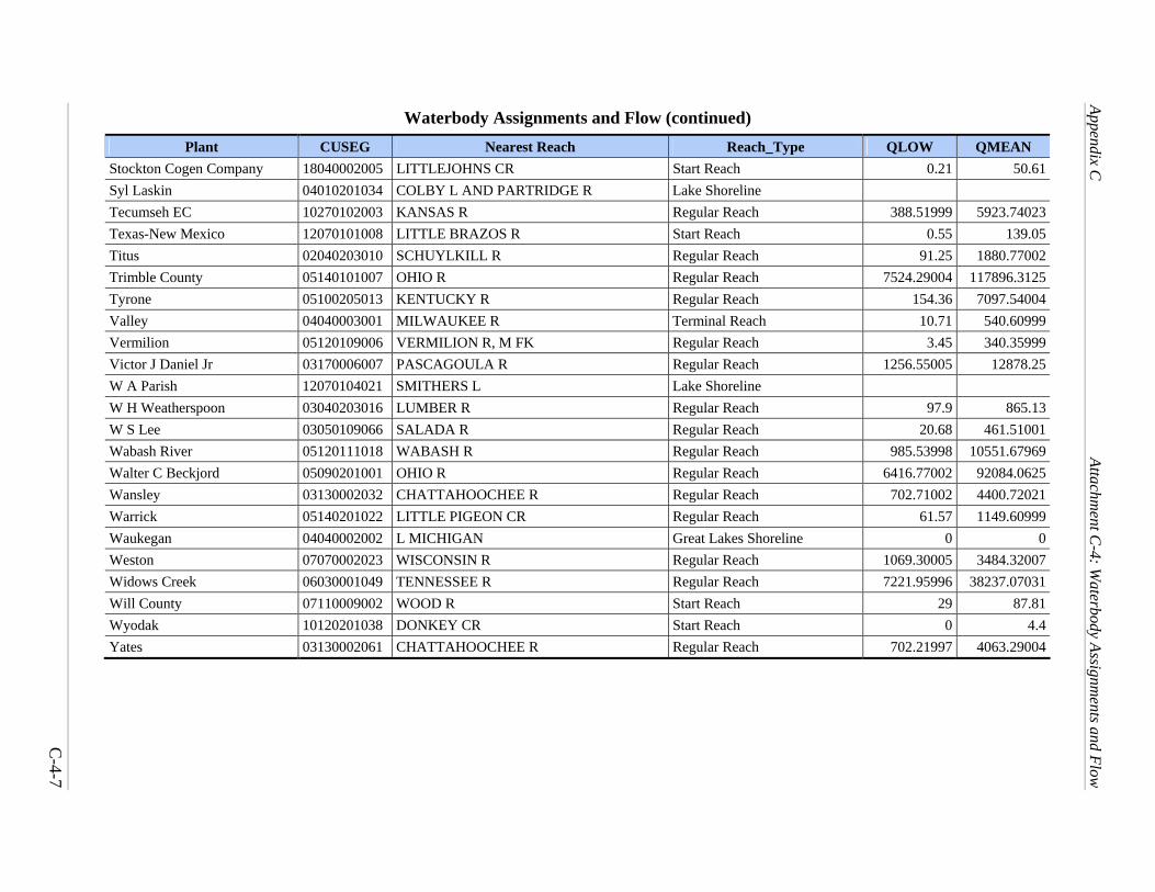
Appendix C
Attachm
ent C-4: W
aterbody Assignments and Flow
C
-4-7
Waterbody Assignments and Flow (continued) Plant CUSEG Nearest Reach Reach_Type QLOW QMEAN
Stockton Cogen Company 18040002005 LITTLEJOHNS CR Start Reach 0.21 50.61Syl Laskin 04010201034 COLBY L AND PARTRIDGE R Lake Shoreline Tecumseh EC 10270102003 KANSAS R Regular Reach 388.51999 5923.74023Texas-New Mexico 12070101008 LITTLE BRAZOS R Start Reach 0.55 139.05Titus 02040203010 SCHUYLKILL R Regular Reach 91.25 1880.77002Trimble County 05140101007 OHIO R Regular Reach 7524.29004 117896.3125Tyrone 05100205013 KENTUCKY R Regular Reach 154.36 7097.54004Valley 04040003001 MILWAUKEE R Terminal Reach 10.71 540.60999Vermilion 05120109006 VERMILION R, M FK Regular Reach 3.45 340.35999Victor J Daniel Jr 03170006007 PASCAGOULA R Regular Reach 1256.55005 12878.25W A Parish 12070104021 SMITHERS L Lake Shoreline W H Weatherspoon 03040203016 LUMBER R Regular Reach 97.9 865.13W S Lee 03050109066 SALADA R Regular Reach 20.68 461.51001Wabash River 05120111018 WABASH R Regular Reach 985.53998 10551.67969Walter C Beckjord 05090201001 OHIO R Regular Reach 6416.77002 92084.0625Wansley 03130002032 CHATTAHOOCHEE R Regular Reach 702.71002 4400.72021Warrick 05140201022 LITTLE PIGEON CR Regular Reach 61.57 1149.60999Waukegan 04040002002 L MICHIGAN Great Lakes Shoreline 0 0Weston 07070002023 WISCONSIN R Regular Reach 1069.30005 3484.32007Widows Creek 06030001049 TENNESSEE R Regular Reach 7221.95996 38237.07031Will County 07110009002 WOOD R Start Reach 29 87.81Wyodak 10120201038 DONKEY CR Start Reach 0 4.4Yates 03130002061 CHATTAHOOCHEE R Regular Reach 702.21997 4063.29004

[This page intentionally left blank.]

Appendix D MINTEQA2 Nonlinear Sorption Isotherms
D-1
Appendix D. MINTEQA2 Nonlinear Sorption Isotherms
D.1 Overview of MINTEQA2 Modeling
Chemicals in leachate can be subject to complex geochemical interactions in soil and groundwater, which can strongly affect their rate of transport in the subsurface. The U.S. Environmental Protection Agency’s Composite Model for Leachate Migration with Transformation Products (EPACMTP) treats these interactions as equilibrium sorption processes. The equilibrium assumption means that the sorption process occurs instantaneously, or at least very quickly relative to the time scale of constituent transport. Although sorption—or the attachment of leachate constituents to solid soil or aquifer particles—may result from multiple chemical processes, EPACMTP lumps these processes together into an effective soil-water partition coefficient (Kd). The retardation factor (R) accounts for the effects of equilibrium sorption of dissolved constituents onto the solid phase. R, a function of the constituent-specific Kd and the soil or aquifer properties, is calculated as:
Φ
ρ1 db K
R×
+= (D-1)
where
R = Retardation factor Db = Soil or aquifer bulk density (mg) Kd = Solid-water partition coefficient (g/cm3) N = Water content (in unsaturated zone) or porosity (in saturated zone).
An isotherm is an expression of the equilibrium relationship between the aqueous concentration and the sorbed concentration of a metal (or other constituent) at a constant temperature. For metals, EPACMTP accounts for more complex geochemical reactions by using effective sorption isotherms generated using EPA’s geochemical equilibrium speciation model for dilute aqueous systems, MINTEQA2 (U.S. EPA, 1991).
The MINTEQA2 model is used to generate one set of isotherms for each metal reflecting the range in geochemical environments expected at waste sites across the nation. The variability in geochemical environments at coal combustion waste (CCW) sites across the country is represented by five geochemical master variables (groundwater composition, pH, concentration of iron oxide adsorption sites, leachate ionic strength, and concentration of dissolved and particulate natural organic matter), and the MINTEQA2 modeling is repeated (separately for each metal) for numerous combinations of master variable settings. This procedure results in nonlinear Kd versus aqueous metal concentration curves for combinations of master variable settings spanning the range of reasonable values (U.S. EPA 2003a).

Appendix D MINTEQA2 Nonlinear Sorption Isotherms
D-2
For each metal, the resulting set of isotherms is tabulated into a supplementary input data file for use by the EPACMTP model, hereafter referred to as an “empirical nonlinear isotherm.” In the fate and transport modeling for a particular metal, EPACMTP is executed and the national probability distributions for these five master variables form the basis for the Monte Carlo selection of the appropriate adsorption isotherm.
In modeling metals transport in the unsaturated zone, EPACMTP uses a range of Kd values from the nonlinear sorption isotherms. However, in modeling metals transport in the saturated zone, EPACMTP selects the lowest from all available Kd values corresponding to concentrations less than or equal to the maximum water table concentration. For more details see the EPACMTP Technical Background Document (U.S. EPA, 2003b).
This simplification in the saturated zone is required for all solution options and is based on the assumption that after dilution of the leachate plume in groundwater, the concentrations of metals will typically be in a range where the isotherm is approximately linear. However, this assumption may not be valid when the metal concentrations in the leachate are exceedingly high. Although EPACMTP is able to account for the effect of the geochemical environment at a site on the mobility of metals, the model assumes that the geochemical environment at a site is constant and not affected by the presence of the leachate plume. In reality, the presence of a leachate plume may alter the ambient geochemical environment.
D.2 Previous CCW Metals Modeling Effort
In a previous risk assessment for fossil fuel combustion wastes (FFCWs) conducted in 1998 (U.S. EPA, 1998), sorption isotherms generated using MINTEQA2 were used in EPACMTP to account for metal partitioning. However, these isotherms were not calculated specifically for use in FFCW modeling—they had been computed using MINTEQA2 in 1995 for use in modeling support for the Hazardous Waste Identification Rule (HWIR).
The disposal scenario for HWIR was the industrial Resource Conservation and Recovery Act (RCRA) Subtitle D nonhazardous waste landfill. In fact, the MINTEQA2 modeling that produced the isotherms had originally been designed to represent municipal solid waste landfills, and leachate from those landfills had been sampled so that appropriate forms of leachate organic acids at various concentrations could be included in the modeling. For the HWIR analysis, the scenario was changed to industrial Subtitle D, and only the isotherms corresponding to low concentrations of the leachate organic acids were used for HWIR modeling. The same isotherms were used in the 1998 FFCW risk assessment. As in the HWIR modeling, only the isotherms corresponding to the lowest setting of leachate organic carbon were used.
In 1999, EPA received review comments concerning the use of the industrial Subtitle D metal partitioning isotherms in the 1998 risk assessment. The most comprehensive review was prepared by Charles Norris and Christina Hubbard on behalf of the Environmental Defense Fund and other environmental advocacy groups (Norris and Hubbard, 1999). The Norris and Hubbard report criticized the 1998 risk assessment for using MINTEQA2 isotherms designed for a different scenario (nonhazardous industrial landfills). Norris and Hubbard also offered 20 specific criticisms on the input parameters and other factors involved in the MINTEQA2 modeling. EPA responded by evaluating each of these criticisms through review and assessment

Appendix D MINTEQA2 Nonlinear Sorption Isotherms
D-3
of MINTEQA2 input values, model sensitivity tests, and consultations with experts. This review is documented in U.S. EPA (2000, 2001a). The evaluation of the Norris and Hubbard comments resulted in suggested revisions in the MINTEQA2 modeling strategy, as described in U.S. EPA (2001b).
Based on a review of available information on CCW leachate composition and an analysis of the potential effects of this composition on metals mobility, EPA (U.S. EPA, 2001b) also determined that if MINTEQA2 is to be used at CCW sites, leachate from CCW facilities should be studied to look for trends in composition, especially with regard to the concentrations of constituents that may
Contribute to elevated groundwater pH
Compete with the contaminant metal for sorption sites and thus result in reduced metal sorption (e.g., Ca, Mg, SO4, other metals)
Complex with the contaminant metal so that the metal is less likely to be sorbed (e.g., SO4, CO3, organic ligands)
Precipitate with the contaminant metal (e.g., SO4, CO3).
D.3 MINTEQA2 Modeling Revisions for CCW Risk Assessment
Many of the suggested revisions from U.S. EPA (2001b) were implemented in the MINTEQA2 modeling for the current CCW risk assessment. Some of the suggested revisions were not implemented, either because they are not applicable (e.g., organic carbon assumptions should not be changed because CCW leachate has negligible organic carbon) or because models or data were not adequate to carry forth the recommendation. These revisions are discussed in greater detail in U.S. EPA (2003c).
In addition to revising the MINTEQA2 model, EPA compiled leachate characteristics into the CCW constituent database (see Appendix A) and statistically analyzed these data to identify three chemically distinct CCW leachate types: conventional CCW (including ash and flue gas desulfurization [FGD] sludge), codisposed CCW and coal cleaning wastes, and fluidized bed combustion (FBC) waste. Leachate concentration ranges for major ions (e.g., Ca, SO4, Mg, Na, Cl, etc.) and pH were developed for each of these waste types and were used to represent CCW leachate during MINTEQA2 modeling.
As needed, sorption reactions were included for those CCW constituents known to undergo significant sorption. Including elevated concentrations of leachate constituents and their corresponding sorption reactions in the MINTEQA2 model allows for full competition with the contaminant metal for sorption sites. The metal solubilizing effect through complexation between the contaminant metal and dissolved ligands is also included, as is the potential for metal precipitation. Because precipitation of the metal can serve to attenuate the transportable concentration, the equilibrium fraction in all three phases (dissolved, sorbed, and precipitated) were stored and made available for use by EPACMTP. The precipitated fraction was used to develop a solubility limit that was used during EPACMTP modeling (U.S. EPA, 2003c).

Appendix D MINTEQA2 Nonlinear Sorption Isotherms
D-4
D.4 MINTEQA2 Modeling for CCW Risk Assessment
The expected natural variability in Kd for a particular metal was represented during the MINTEQA2 modeling effort by varying the input parameters that most impact Kd: groundwater type (carbonate or noncarbonate), pH, concentration of aquifer sorbents, composition and concentration level of CCW leachate, and concentration of the contaminant metal. The natural pH range for the two groundwater types was sampled from a range of 7 to 8 for carbonate aquifers and 4 to 10 for noncarbonate aquifers (U.S. EPA, 2003c).
In addition, CCW leachate ranges from acidic (pH < 2) to highly alkaline (pH > 12) and can impact vadose zone and groundwater pH. To account for this possibility, the CCW leachate/ groundwater system was equilibrated at a series of pH values that span the range of expected variability in mixed CCW leachate-groundwater systems (U.S. EPA, 2003c).
To account for the variability in the sorption capacity of soil and aquifer materials, the soil and groundwater systems were equilibrated with various concentrations of two commonly occurring natural sorbents: ferric (iron) oxyhydroxide (FeOx) and particulate organic matter (POM). CCW leachate can include elevated concentrations of inorganic constituents such as calcium, sulfate, sodium, potassium, and chloride, which may reduce sorption of metals due to competition for sorption sites or complexation with metals in solution. To account for this effect, these leachate components were added to the MINTEQA2 model inputs at concentrations representative of the three CCW waste types (conventional CCWs, codisposed CCW and coal cleaning wastes, and FBC wastes). This new MINTEQA2 master variable is termed leachate “richness” or ionic strength (U.S. EPA, 2003c).
The results of each MINTEQA2 model run were compiled as the equilibrium distribution of the contaminant metal among dissolved, sorbed, and precipitated fractions for each metal concentration, and were saved in a separate file indexed with the settings of all variables used to define the system. These files were produced for all possible values for the variables defining the system, and were compiled into a database of indexed Kd values for use in the EPACMTP fate and transport model (U.S. EPA, 2003c).
D.5 EPACMTP Modeling Revisions to Accommodate MINTEQA2 Updates
EPA updated EPACMTP to support the new system variable (leachate ionic strength) for isotherm selection, to address issues regarding the impacts of leachate pH on ambient soil and aquifer pH, and to address issues regarding solubility limits for metals in solution. A brief description of these model changes are discuss below, with more detail provided in U.S. EPA (2003d).
Ionic Strength. A new system or “master” variable was added to include ionic strength as a key for choosing the representative isotherm from the database for both the unsaturated and saturated zones.
Leachate Effects on Geochemical Environment. These effects were addressed in EPACMTP under the following constraints: (1) no significant impairment of the computational efficiency for probabilistic applications; (2) data requirements limited to readily available data;

Appendix D MINTEQA2 Nonlinear Sorption Isotherms
D-5
and (3) a scientifically defensible approach, given significant uncertainties with respect to the true impacts of leachate pH on the subsurface. Two modifications to the EPACMTP were considered: (1) determine the governing pH in the soil column (either the pH of the leachate or the native soils); and (2) determine the pH of the saturated zone as a result of the infiltrating leachate.
The approach selected for determining the governing pH of the soil column (vadose zone) beneath the waste management unit (WMU) compares the operational life of the WMU (the duration of leaching) to an estimate of the first arrival time of the contaminant front at the water table (a surrogate for the residence time of the contaminant in the soil column). If the operational life of the WMU is relatively long compared to the time required for the contaminant to migrate to the water table, there is a high likelihood that the leachate permeates the soil column and that the pH environment is governed by the leachate.
Conversely, a relatively short operational life and retarded contaminant migration would favor ambient soil pH conditions. An analysis of the relationship between operational life and travel time indicated that a ratio of approximately 5 (operational life over travel time) would, in many cases, result in a balanced selection of cases where leachate pH governs versus cases where soil pH governs over approximately 10,000 Monte Carlo iterations.
For each iteration of EPACMTP, the operational life was compared to a travel-time estimate based on a Kd averaged from isotherms selected based on the leachate pH and soil pH. If the ratio was greater than 5, the pH of the leachate was assumed to govern, and the pH of the leachate was used to select the isotherm for transport in the unsaturated zone. If the ratio was less than 5, the soil pH was used to select the isotherm.
In the saturated zone, the impacts of leachate pH were handled using a simple homogeneous mixing calculation. The volume of leachate released from the WMU was mixed with the volume of the aquifer that was likely to be impacted by a plume. The resulting mixed pH was used to select the isotherm for transport in the saturated zone with one limitation: in carbonate environments, the mixed pH in the aquifer was not allowed to drop below a pH of 6. Such acid conditions would likely result in significant dissolution of the soil matrix.
Metal Solubility Limits. As mentioned above, each sorption isotherm comprises equilibrium concentrations of the three contaminant phases (dissolved, sorbed, and precipitated) over a range of total concentration values. An examination of the change in the dissolved-phase concentrations relative to changes in the total concentration in any isotherm reveals solubility behavior for that contaminant: if the dissolved component does not change with increasing total concentration, a solubility limit has been achieved. If, however, the dissolved component increases along with the total concentration, then there is capacity for more dissolved mass in the groundwater or soil porewater.
EPACMTP uses this information (contained in each isotherm file) to determine if a solubility limit should be imposed in the saturated zone. Once an isotherm has been selected (after pH considerations have been addressed), the equilibrium states corresponding to the three highest total concentrations are examined. If the dissolved concentration changes more than one tenth of one percent over the last three points, then EPACMTP assumes there is no solubility

Appendix D MINTEQA2 Nonlinear Sorption Isotherms
D-6
limit. If the change in dissolved concentration is less than one tenth of one percent, EPACMTP assumes a solubility limit has been reached and caps the concentration of the leachate entering the saturated zone at the water table to that limit.
D.5 References
Norris, C.H., and C.E. Hubbard. 1999. Use of MINTEQA2 and EPACMTP to Estimate Groundwater Pathway Risks from the Land Disposal of Metal-Bearing Wastes. Prepared for The Environmental Defense Fund, Friends of the Earth, Hoosier Environmental Council, and Mineral Policy Center.
U.S. EPA (Environmental Protection Agency). 1991. MINTEQ2A/PRODEF2A, A Geochemical Assessment Model for Environmental Systems: Version 3.0 User’s Manual. EPA/600/3-91/021. Office of Research and Development, Athens, GA.
U.S. EPA (Environmental Protection Agency). 1998. Methodology for Assessing Health Risks Associated with Multiple Pathways of Exposure to Combustor Emissions. Update to Methodology for Assessing Health Risks Associated with Indirect Exposure to Combustor Emissions. EPA-600/R-98/137. National Center for Environmental Assessment, Cincinnati, OH.
U.S. EPA (Environmental Protection Agency). 2000. Discussion and Recommendations Concerning Comments Received by the U.S. EPA on the EPACMTP and MINTEQA2 Models as Used in Modeling Support for FFCW Rulemaking. Prepared by Allison Geoscience Consultants, Inc. for the Office of Solid Waste, Washington, DC.
U.S. EPA (Environmental Protection Agency). 2001a. Modeling Sensitivity Analyses Concerning Comments Received by the U.S. EPA on the MINTEQA2 Model as Used in Modeling Support for FFCW Rulemaking. Prepared by Allison Geoscience Consultants, Inc., for the Office of Solid Waste, Washington, DC.
U.S. EPA (Environmental Protection Agency). 2001b. Revisions in Input Data and Modeling Procedures for Using MINTEQA2 in Estimating Metal Partition Coefficients. Prepared by Allison Geoscience Consultants, Inc., for the Office of Solid Waste, Washington, DC.
U.S. EPA (Environmental Protection Agency). 2003a. EPACMTP Parameters/Data Document. Office of Solid Waste, Washington, DC.
U.S. EPA (Environmental Protection Agency). 2003b. EPACMTP Technical Background Document. Office of Solid Waste, Washington, DC.
U.S. EPA (Environmental Protection Agency). 2003c. Estimation of Metal Partition Coefficients for Fossil Fuel Combustion Waste Risk Assessment. Prepared by Allison Geoscience Consultants, Inc. (under subcontract to RTI International) for U.S. EPA. June.
U.S. EPA (Environmental Protection Agency). 2003d. Addendum to the EPACMTP Technical Background Document. Office of Solid Waste, Washington, DC.

Appendix E Equations
E-1
Appendix E. Surface Water, Fish Concentration, and Contaminant Intake Equations
This appendix presents the equations used to model surface water and fish concentrations and intake of drinking water and fish. These equations are presented in the following attachments:
Attachment E-1 provides the equations comprising the surface water equilibrium partitioning model, including equations that estimate steady state concentrations in the water column (dissolved and total) and sediments.
Attachment E-2 provides the equations that use bioconcentration factors (BCFs) to calculate fish tissue concentrations from total.
Attachment E-3 provides the equations used to calculate daily contaminant intake rates from drinking water and fish consumption.
E.1 Aluminum Surface Water Precipitation Because the fate and transport of aluminum is controlled more by solubility than by sorption in surface water, the surface water model includes algorithms to estimate aluminum concentrations in the water column and sediments by accounting for precipitation and fallout of aluminum in the water column. These calculations proceed in a stepwise fashion, as follows. Step 1. Initially, assume all influent aluminum is dissolved in the water column. Fraction in water column (fwater) = 1 Fraction in sediment layer (fbenth) = 0 Fraction dissolved (fd) = 1 Total water column concentration (Cwctot) = dissolved water column concentration (Cwd). Step 2. Compare the dissolved water column concentration (Cwd) to the maximum soluble concentration (Csol) calculated in MINTEQA2 for the waterbody pH (see Section 3.5.4, Table 3-6 for aluminum solubilities and Appendix C, Section C.6.3, Table C-11 for waterbody pH). Step 3. If the dissolved water concentration (Cwd) is greater than the solubility limit (Csol), reset the dissolved water concentration to the solubility limit, and precipitate and settle out the excess aluminum to the benthic sediment layer.

Appendix E Equations
E-2
If Cwctot > Csol, then Fwater = Csol / Cwctot Fbenth = (Cwctot - Csol) / Cwctot Cwbs = (Cwctot - Csol) * dwc / db Cwtot = Cwctot * dwc / dz Cdw = Csol Cwctot = Csol Else Cdw = Cwctot Cwbs = 0 Cwtot = Cwctot * rsParam!dwc / rsParam!dz End If where: Cdw = issolved waterbody concentration Csol = maximum soluble concentration Cwbs = total concentration in bed sediment Cwtot = total waterbody concentration from loading db = depth of the upper benthic layer dwc = depth of the water column dz = depth of the waterbody fbenth = fraction in sediment layer fd = fraction dissolved fwater = fraction in water column

Table E-1-1. Fraction of Contaminant in Water Column (unitless)
Name Description Value
Appendix E
fWater
Attachment E-1: Surface Water Concentrations
bzw ddd −=
( )[ ]
( )[ ] ( ) ��
���
�××++�
�
���
�×××+
×××+=
z
bdbs
z
wdsw
z
wdsw
Water
dd
bscKbspdd
TSSK
dd
TSSKf
000001.01
000001.01
bsc Bed sediment particle concentration (g/cm^3) or (kg/L) 1
bsp Bed sediment porosity (cm^3/cm^3) 0.6
Depth of upper benthic layer (m)db 0.03
Depth of water column (m)dw Site Data; See Appendix C
Depth of the waterbody (m)dz Calculated
Sedment-water partition coefficient (mL/g)Kdbs Chemical Data; See Section 3
Suspended sediment-water partition coefficient (mL/g)Kdsw Chemical Data; See Section 3
Total suspended solids (mg/L)TSS Site Data; See Appendix C
0.000001 Conversion factor (L/ml)(g/mg)
E-1-1

Table E-1-2. Fraction of Contaminant in Benthic Sediments (unitless)
Name Description Value
Appendix E
fBenth
Attachment E-1: Surface Water Concentrations
( )
( ) ( ) ��
���
�××++�
�
���
�×××+
××+=
z
bdbs
z
Wdsw
z
bdbs
Benth
dd
bscKbspdd
TSSK
dd
bscKbspf
000001.01
bsc Bed sediment particle concentration (g/cm^3) or (kg/L) 1
bsp Bed sediment porosity (cm^3/cm^3) 0.6
Depth of upper benthic layer (m)db 0.03
Depth of water column (m)dw Site Data; See Appendix C
Depth of the waterbody (m)dz Calculated
Sedment-water partition coefficient (mL/g)Kdbs Chemical Data; See Section 3
Suspended sediment-water partition coefficient (mL/g)Kdsw Chemical Data; See Section 3
Total suspended solids (mg/L)TSS Site Data; See Appendix C
0.000001 Conversion factor (L/ml)(g/mg)
E-1-2

Table E-1-3. Dissolved Fraction (unitless)
Name Description Value
Appendix E
fd
Attachment E-1: Surface Water Concentrations
000001.011
××+=
TSSKf
dswd
Suspended sediment-water partition coefficient (mL/g)Kdsw Chemical Data; See Section 3
Total suspended solids (mg/L)TSS Site Data; See Appendix C
0.000001 Conversion factor (L/ml)(g/mg)
E-1-3

Table E-1-4. Water Concentration Dissipation Rate Constant (1/d)
Name Description Value
Appendix E
Kwt
Attachment E-1: Surface Water Concentrations
( ) ( ) ( ) ( ) hsedbenthswWaterbbenthvoldWaterwt kkfkfKfkffK +×+×+×+××=
bb d
WBK =
w
vvol d
Kk =
Depth of upper benthic layer (m)db 0.03
Depth of water column (m)dw Site Data; See Appendix C
Fraction of contaminant in benthic sediments (unitless)Fb Calculated
Dissolved fraction (unitless)fd Calculated
Fraction of contaminant in water column (unitless)fWater Calculated
Benthic burial rate constant (1/day)Kb Calculated
Hydrolysis rate (1/day)kh 0
Degradation rate for sediment (1/day)ksed 0
Degradation rate for water column (1/day)ksw 0
Diffusion transfer rate (m/day)Kv Calculated (mercury only)
Water column volatilization rate constant (1/day)kvol Calculated (mercury only)
WB Rate of Burial (m/day) 0
E-1-4

Table E-1-5. Total Waterbody Concentration from Loading (g/m^3 or mg/L)
Name Description Value
Appendix E
CwTot
Attachment E-1: Surface Water Concentrations
zWB dAreaV ×=
VKdd
fV
LCw
wtw
zWaterfx
totalTot
×+××=
Area of the waterbody (m^2)AreaWB Site Data; See Appendix C
Depth of upper benthic layer (m)db 0.03
Depth of water column (m)dw Site Data; See Appendix C
Depth of the waterbody (m)dz Calculated
Fraction of contaminant in water column (unitless)fWater Calculated
Water Concentration Dissipation Rate Constant (1/day)Kwt Calculated
Total waterbody load (g/day)LTotal Calculated By EPACMTP
Flow independent mixing volume (m^3)V Calculated
Waterbody annual flow mixing volume (m3/day)Vfx Site Data; See Appendix C
E-1-5

Table E-1-6. Total Water Column Concentration (g/m^3 or mg/L)
Name Description Value
Appendix E
CwcTot
Attachment E-1: Surface Water Concentrations
bzw ddd −=
w
zwaterwTotwcTot d
dfCC ××=
Total Waterbody Concentration from Loading (g/m^3 or mg/L)CwTot Calculated
Depth of upper benthic layer (m)db 0.03
Depth of water column (m)dw Site Data; See Appendix C
Depth of the waterbody (m)dz Calculated
Fraction of contaminant in water column (unitless)fWater Calculated
E-1-6

Table E-1-7. Dissolved Waterbody Concentration (mg/L)
Name Description Value
Appendix E
Cdw
Attachment E-1: Surface Water Concentrations
bzw ddd −=
w
ZdWaterTotdw d
dffCwC ×××=
Total Waterbody Concentration from Loading (g/m^3 or mg/L)CwTot Calculated
Depth of upper benthic layer (m)db 0.03
Depth of water column (m)dw Site Data; See Appendix C
Depth of the waterbody (m)dz Calculated
Dissolved fraction (unitless)fd Calculated
Fraction of contaminant in water column (unitless)fWater Calculated
E-1-7

Table E-1-8. Total Concentration in Bed Sediment (g/m^3 or mg/L)
Name Description Value
Appendix E
Cwbs
Attachment E-1: Surface Water Concentrations
bwz ddd +=
b
zbenthTotwbs d
dfCC ××=
Total Waterbody Concentration from Loading (g/m^3 or mg/L)CwTot Calculated
Depth of upper benthic layer (m)db 0.03
Depth of water column (m)dw Site Data; See Appendix C
Depth of the waterbody (m)dz Calculated
E-1-8

Table E-2-1. Concentration in Fish at Different Trophic Levels (mg/kg)
Name Description Value
Appendix E
Cfish
Attachment E-2: Fish Concentrations
For Non-Volatile Metals:
BCFCwC totfish ×=
BCF Chemical Data; See Section 3Bioconcentration factor for specified trophic level (L/kg)
CalculatedDissolved waterbody concentration (mg/L)Cdw CalculatedTotal waterbody concentration from loading (g/m^3 or mg/L)CwTot
0.15 Fraction of dissolved mercury assumed to be methyl mercury (unitless)
E-2-1

Table E-2-2. Average Fish Fillet Concentration Ingested by Humans (mg/kg)
Name Description Value
Appendix E
Cfish_fillet
Attachment E-2: Fish Concentrations
FfishTTFfishTTfilletfish CFCFC 4433_ ×+×=
CalculatedConcentration of contaminant in fish at different trophic levels (mg/kg)
CfishT3F
CalculatedConcentration of contaminant in fish at different trophic levels (mg/kg)
CfishT4F
0.36Fraction of trophic level 3 intake (unitless)FT3
0.64Fraction of trophic level 4 intake (unitless)FT4
E-2-2

Table E-3-1. Contaminant Intake from Drinking Water (mg/kg-d)
Name Description Value
Appendix E
Idw
Attachment E-3: Intake Rates
1000*BWFCRC
I dwdwdwdw
××=
BW Exposure Data; See Appendix FBody weight (kg)
CalculatedDissolved waterbody concentration (mg/L)Cdw Exposure Data; See Appendix FConsumption rate of water (mL/day)CRdw
1Fraction of drinking water ingested that is contaminated (unitless)
Fdw
1000 Conversion factor (mL/L)
E-3-1

Table E-3-2. Daily Intake of Contaminant from Fish Ingestion (mg/kg BW/day)
Name Description Value
Appendix E
Ifish
Attachment E-3: Intake Rates
BW
FCRCI fishfishfilletfish
fish ×××
=1000
_
BW Exposure Data; See Appendix FBody weight (kg)
CalculatedAverage fish fillet concentration ingested by humans (mg/kg)Cfish_fillet Exposure Data; See Appendix FConsumption rate of fish (g WW/day)CRfish
1Fraction of fish intake from contaminated source (unitless)Ffish
1000 Conversion factor (g/kg)
E-3-2

Appendix F Human Exposure Factors
F-1
Appendix F. Human Exposure Factors
Exposure factors are data that quantify human behavior patterns (e.g., ingestion rates of fish and drinking water) and characteristics (e.g., body weight) that affect a person’s exposure to environmental contaminants. These data can be used to construct realistic assumptions concerning an individual’s exposure to and subsequent intake of a contaminant in the environment. The exposure factors data also enable the U. S. Environmental Protection Agency (EPA) to differentiate the exposures of individuals of different ages (e.g., a child vs. an adult). The derivation and values used for the human exposure factors in this risk assessment are described below, and the exposure factors selected for the probabilistic analyses are also presented.
F.1 Exposure Parameters Used in Probabilistic Analysis
F.1.1 Introduction
The general methodology for collecting human exposure data for the probabilistic analysis relied on the Exposure Factors Handbook, or EFH (U.S. EPA, 1997a-c), which was used in one of three ways:
1. When EFH percentile data were adequate (most input variables), maximum likelihood estimation was used to fit selected parametric models (gamma, lognormal, Weibull, and generalized gamma) to the EFH data. The chi-square measure of goodness of fit was then used to choose the best distribution. Parameter uncertainty information (e.g., for averages, standard deviations) also was derived using the asymptotic normality of the maximum likelihood estimate or a regression approach.
2. When EFH percentile data were not adequate for statistical model fitting (a few variables), models were selected on the basis of results for other age cohorts or, if no comparable information was available, by assuming lognormal as a default distribution and reasonable coefficients of variation (CVs).
3. When data were not adequate for either 1 or 2 above, variables were fixed at EFH-recommended mean values or according to established EPA policy.
Table F-1 lists all of the parameters used in the probabilistic analysis. Both fixed variables and the values used to define distributed data are provided.
Probabilistic risk analyses involve “sampling” values from probability distribution functions (PDFs) and using the values to estimate risk. In some cases, distributions are infinite, and there is a probability, although very small, that very large or very small values might be selected from the distributions. Because selecting extremely large or extremely small values is unrealistic (e.g., the range of adult body weights is not infinite), maximum and minimum values

Appendix F Human Exposure Factors
F-2
were imposed on the distributions. The minimum and maximum values are included in Table F-1.
F.1.2 Exposure Parameter Distribution Methodology
This section describes how stochastic or distributed input data for each exposure factor were collected and processed. Exposure parameter distributions were developed for use in the Monte Carlo analysis. For most variables for which distributions were developed, exposure factor data from the EFH were analyzed to fit selected parametric models (i.e., gamma, lognormal, Weibull). Steps in the development of distributions included preparing data, fitting models, assessing fit, and preparing parameters to characterize distributional uncertainty in the model inputs.
For many exposure factors, EFH data include sample sizes and estimates of the following parameters for specific receptor types and age groups: mean, standard deviation, standard error, and percentiles corresponding to a subset of the following probabilities: 0.01, 0.02, 0.05, 0.10, 0.15, 0.25, 0.50, 0.75, 0.85, 0.90, 0.95, 0.98, and 0.99. These percentile data, where available, were used as a basis for fitting distributions. Although in no case were all of these percentiles actually provided for a single factor, seven or more are typically present in the EFH data. Therefore, using the percentiles is a fuller use of the available information than fitting distributions simply based on the method of moments (e.g., selecting models that agree with the data mean and standard deviation). For some factors, certain percentiles were not used in the fitting process because sample sizes were too small to justify their use. Percentiles were used only if at least one data point was in the tail of the distribution. If the EFH data repeated a value across several adjacent percentiles, only one value (the most central or closest to the median) was used in most cases (e.g., if both the 98th and 99th percentiles had the same value, only the 98th value was used).
The EFH does not use standardized age cohorts across exposure factors. Different exposure factors have data reported for different age categories. Therefore, to obtain the percentiles for fitting the four standardized age cohorts (i.e., ages 1 to 5, 6 to 11, 12 to 19, and more than 20), each EFH cohort-specific value for a given exposure factor was assigned to one of these four cohorts. When multiple EFH cohorts fit into a single cohort, the EFH percentiles were averaged within each cohort (e.g., data on 1- to 2-year-olds and 3- to 5-year-olds were averaged for the 1- to 5-year-old cohort). If sample sizes were available, weighted averages were used, with weights proportional to sample sizes. If sample sizes were not available, equal weights were assumed (i.e., the percentiles were simply averaged).

Appendix F H
uman Exposure Factors
F-3
Table F-1. Summary of Exposure Parameters Used in Probabilistic Analysis
Parameter Units Variable
Type Constants Mean
(or shape) Std Dev
(or scale) Minimum Maximum Reference Averaging time for carcinogens yr Constant 7.00E+01 U.S. EPA (1989) Body weight (adult) kg Lognormal 7.12E+01 1.33E+01 1.50E+01 3.00E+02 U.S. EPA (1997a); Tables 7-2,
7-4, 7-5 Body weight (child 1) kg Lognormal 1.55E+01 2.05E+00 4.00E+00 5.00E+01 U.S. EPA (1997b); Tables 7-3,
7-6, 7-7 Body weight (child 2) kg Lognormal 3.07E+01 5.96E+00 6.00E+00 2.00E+02 U.S. EPA (1997a); Tables 7-3,
7-6, 7-7 Body weight (child 3) kg Lognormal 5.82E+01 1.02E+01 1.30E+01 3.00E+02 U.S. EPA (1997a); Tables 7-3,
7-6, 7-7 Consumption rate: fish (adult, child) g/d Lognormal 6.48E+00 1.99E+01 0.00E+00 1.50E+03 U.S. EPA (1997b); Table 10-64 Exposure duration (adult resident) yr Weibull 1.34E+00 1.74E+01 1.00E+00 5.00E+01 U.S. EPA (1999) (ACS) Exposure duration (child) yr Weibull 1.32E+00 7.06E+00 1.00E+00 5.00E+01 U.S. EPA (1999) (ACS) Exposure frequency (adult resident) d/yr Constant 3.50E+02 U.S. EPA Policy Fraction contaminated: drinking water Fraction Constant 1.00E+00 U.S. EPA Policy Fraction contaminated: fish Fraction Constant 1.00E+00 U.S. EPA Policy Fraction of fish consumed that is trophic level (T3) fish
Fraction Constant 3.60E-01 U.S. EPA (1997b); Table 10-66
Fraction of fish consumed that is trophic level 4 (T4) fish
Fraction Constant 6.40E-01 U.S. EPA (1997b); Table 10-66
Ingestion rate: drinking water (adult resident)
mL/d Gamma 3.88E+00 3.57E+02 1.04E+02 1.10E+04 U.S. EPA (1997a); Table 3-6
Ingestion rate: drinking water (child 1 resident)
mL/d Gamma 2.95E+00 2.37E+02 2.60E+01 3.84E+03 U.S. EPA (1997a); Table 3-6
Ingestion rate: drinking water (child 2 resident)
mL/d Gamma 3.35E+00 2.35E+02 3.40E+01 4.20E+03 U.S. EPA (1997a); Table 3-6
Ingestion rate: drinking water (child 3 resident)
mL/d Gamma 2.82E+00 3.42E+02 3.30E+01 5.40E+03 U.S. EPA (1997a); Table 3-6

Appendix F Human Exposure Factors
F-4
Because the EFH data are always positive and are almost always skewed to the right (i.e., have a long right tail), three two-parameter probability models commonly used to characterize such data (gamma, lognormal, and Weibull) were selected. In addition, a three-parameter model (generalized gamma) was used that unifies them1 and allows for a likelihood ratio test of the fit of the two-parameter models. However, only the two-parameter models were selected for use in the analysis because the three-parameter generalized gamma model did not significantly improve the goodness of fit over the two-parameter models. This simple setup constitutes a considerable improvement over the common practice of using a lognormal model in which adequate EFH data are available to support maximum likelihood estimation.
Lognormal, gamma, Weibull, and generalized gamma distributions were fit to each factor data set using maximum likelihood estimation (Burmaster and Thompson, 1998). When sample sizes were available, the goodness of fit was calculated for each of the four models using the chi-square test (Bickel and Doksum, 1977). When percentile data were available but sample sizes were unknown, a regression F-test for the goodness of fit against the generalized gamma model was used. For each of the two-parameter models, parameter uncertainty information (i.e., mean, standard deviation, scale, and shape) was provided as parameter estimates for a bivariate normal distribution that could be used for simulating parameter values (Burmaster and Thompson, 1998). The information necessary for such simulations includes estimates of the two model parameters, their standard errors, and their correlation. To obtain this parameter uncertainty information, the asymptotic normality of the maximum likelihood estimate (Burmaster and Thompson, 1998) was used when sample sizes were available, and a regression approach was used when sample sizes were not available (Jennrich and Moore, 1975; Jennrich and Ralston, 1979). In either case, uncertainty can be expressed as a bivariate normal distribution for the model parameters.
Section F.1.3 discusses fixed parameters. Section F.1.4 describes, for each exposure factor, the EFH data used to develop the distributions, along with the final distributional statistics.
F.1.3 Fixed Parameters
Certain parameters were fixed, based on central tendency values from the best available source (usually EFH recommendations), either because no variability was expected or because the available data were not adequate to generate distributions. Fixed (constant) parameters are shown in Table F-2 along with the value selected for the risk analysis and the data source. These constants include variables for which limited or no percentile data were provided in the EFH: exposure frequency, fractions of T3 and T4 fish consumed, and fraction contaminated for the various media. Most of these values were extracted directly from the EFH. When evaluating carcinogens, total dose is averaged over the lifetime of the individual, assumed to be 70 years.
1 Gamma, Weibull, and lognormal distributions are all special cases of the generalized gamma distribution.

Appendix F Human Exposure Factors
F-5
Table F-2. Summary of Human Exposure Factor Data Used in Modeling: Constants
Description Value Units Source Fraction contaminated: drinking water 1 Fraction EPA policy Fraction contaminated: fish 1 Fraction EPA policy Fraction of T3 fish consumed 0.36 Fraction U.S. EPA (1997b); Table 10-66 Fraction of T4 fish consumed 0.64 Fraction U.S. EPA (1997b); Table 10-66 Exposure frequency (adult, child) 350 d/yr EPA policy Averaging time for carcinogens (adult, child) 70 yr U.S. EPA (1989)
The fraction contaminated for drinking water was assumed to be 1 (i.e., all drinking water available for consumption at a site is potentially contaminated), with actual concentrations depending on fate and transport model results. Thus, households for which the drinking water pathway was analyzed were assumed to get 100 percent of their drinking water from groundwater. Exposure frequency was set to 350 days per year in accordance with EPA policy, assuming that residents take an average of 2 weeks’ vacation time away from their homes each year.
F.1.4 Variable Parameters
F.1.4.1 Fish Consumption
Table F-3 presents fish consumption data and distributions. Fish consumption data were obtained from Table 10-64 of the EFH (U.S. EPA, 1997b). Data (in g/d) were available for adult freshwater anglers in Maine. The Maine fish consumption study was one of four recommended freshwater angler studies in the EFH (U.S. EPA, 1997b). The other recommended fish consumption studies (i.e., Michigan and New York) had large percentages of anglers who fished from Great Lakes, which is not consistent with the modeling scenarios used in this risk analysis. The anglers in the Maine study fished from streams, rivers, and ponds; these data are more consistent with our modeling scenarios. Although the Maine data have a lower mean than the Michigan data, the Maine data compared better with a national U.S. Department of Agriculture (USDA) study. Also, the Maine study included percentile data, which were necessary to develop a distribution.
Percentile data were used to fit parametric models (gamma, lognormal, and Weibull), and measures of goodness of fit were used to select lognormal as the most appropriate model. The fraction of fish intake that is locally caught was assumed to be 1 (in accordance with EPA policy). The fraction of consumed T3 and T4 fish was 0.36 and 0.64, respectively (Table 10-66, U.S. EPA, 1997b).
Table F-3. Fish Consumption Data and Distribution
EFH Data (g/d) Distribution Age Cohort
N
Data Mean
Data SD
P50
P66
P75
P90
P95
Distribution
Pop-Estd Mean
Pop-Estd SD
All ages 1,053 6.4 2 4 5.8 13 26 Lognormal 6.48 19.9 N = Number of samples; P50–P95 = Percentiles; Pop-Estd = Population-estimated; SD = Standard deviation.

Appendix F Human Exposure Factors
F-6
F.1.4.2 Drinking Water Intake
Table F-4 presents drinking water intake data and distributions. Drinking water intake data were obtained from Table 3-6 of the EFH (U.S. EPA, 1997a). Data (in mL/d) were presented by age groups. Weighted averages of percentiles, means, and standard deviations were calculated for the three child age groups and adults. Percentile data were used to fit parametric models (gamma, lognormal, and Weibull) using maximum likelihood estimation. Measures of goodness of fit were used to select the most appropriate model. The fraction of drinking water contaminated was assumed to be 1 (in accordance with EPA policy).
Table F-4. Drinking Water Intake Data and Distributions
EFH Data (mL/d) Distributions
Age
Cohort
N
Data Mean
Data SD
P01
P05
P10
P25
P50
P75
P90
P95
P99
Distribution
Pop- Estd Mean
Pop- Estd SD
1–5 3,200 697.1 401.5 51.62 187.6 273.5 419.2 616.5 900.8 1,236 1,473 1,917 Gamma 698 406
6–11 2,405 787 417 68 241 318 484 731 1,016 1,338 1,556 1,998 Gamma 787 430
12–19 5,801 963.2 560.6 65.15 241.4 353.8 574.4 868.5 1,247 1,694 2,033 2,693 Gamma 965 574
20+ 13,394 1,384 721.6 207.6 457.5 607.3 899.6 1,275 1,741 2,260 2,682 3,737 Gamma 1,383 703
N = Number of samples; P01–P99 = Percentiles; Pop-Estd = Population-estimated; SD = Standard deviation.
F.1.4.3 Body Weight
Table F-5 presents body weight data and distributions. Body weight data were obtained from Tables 7-2 through 7-7 of the EFH (U.S. EPA, 1997a). Data (in kg) were presented by age and gender. Weighted averages of percentiles, means, and standard deviations were calculated for 1- to 5-year-olds, 6- to 11-year-olds, 12- to 19-year olds, and adult age groups; male and female data were weighted and combined for each age group. These percentile data were used as the basis for fitting distributions. These data were analyzed to fit parametric models (gamma, lognormal, and Weibull) using maximum likelihood estimation. Measures of goodness of fit were used to select the most appropriate model.
Table F-5. Body Weight Data and Distributions
EFH Data (kg) Distributions
Age Cohort N
Data Mean
Data SD P05 P10 P15 P25 P50 P75 P85 P90 P95 Distribution
Pop- Estd
Mean
Pop- Estd SD
1–5 3,762 15.52 3.719 12.5 13.1 13.45 14.03 15.26 16.67 17.58 18.32 19.45 Lognormal 15.5 2.05
6–11 1,725 30.84 9.561 22.79 24.05 25.07 26.44 29.58 33.44 36.82 39.66 43.5 Lognormal 30.7 5.96
12–19 2,615 58.45 13.64 43.84 46.52 48.31 50.94 56.77 63.57 68.09 71.98 79.52 Lognormal 58.2 10.2
20+ 12,504 71.41 15.45 52.86 55.98 58.21 61.69 69.26 78.49 84.92 89.75 97.64 Lognormal 71.2 13.3
N = Number of samples; P05–P95 = Percentiles; Pop-Estd = Population-estimated; SD = Standard deviation.

Appendix F Human Exposure Factors
F-7
F.1.4.4 Exposure Duration
Table F-6 presents exposure duration data and distributions. Exposure duration was assumed to be equivalent to the average residence time for each receptor. Exposure durations for adult and child residents were determined using data on residential occupancy from the EFH Table 15-168 (U.S. EPA, 1997c). The data represent the total time a person is expected to live at a single location, based on age. The table presents male and female data combined. Adult residents aged 21 to 90 were pooled. For child residents, the 3-year-old age group was used for the 1- to 5-year-olds. The 6- and 9-year-old age groups were pooled for the 6- to 11-year-old cohort.
Table F-6. Exposure Duration Data and Distributions
EFH Data Distributions
Age Cohort Data Mean
(yr)
Distribution Pop-Estd Shape
(yr)a Pop-Estd Scale
(yr) 1–5 6.5 Weibull 1.32 7.059 6–11 8.5 Weibull 1.69 9.467 Adult 16.0 Weibull 1.34 17.38 Pop-Estd = Population-estimated. a Distributions used in risk assessment.
In an analysis of residential occupancy data, Myers et al. (U.S. EPA, 2000) found that the data, for most ages, were best fit by a Weibull distribution. The Weibull distribution as implemented in Crystal Ball® is characterized by three parameters: location, shape, and scale. Location is the minimum value and, in this case, was presumed to be 0. Shape and scale were determined by fitting a Weibull distribution to the pooled data, as follows. To pool residential occupancy data for the age cohorts, an arithmetic mean of data means was calculated for each age group. Then, assuming a Weibull distribution, the variance within each age group (e.g., 6-year-olds) was calculated in the age cohort. These variances in turn were pooled over the age cohort using equal weights. This is not the usual type of pooled variance, which would exclude the variation in the group means. However, this way, the overall variance reflected the variance of means within the age groups (e.g., within the 6-year-old age group). The standard deviation was estimated as the square root of the variance. The coefficient of variation was calculated as the ratio of the standard deviation divided by the Weibull mean. For each cohort, the population-estimated parameter uncertainty information (e.g., shape and scale) was calculated based on a Weibull distribution, the calculated data mean for the age cohort, and the CV.
F.2 References
Bickel, P.J., and K.A. Doksum. 1977. Mathematical Statistics. San Francisco, CA: Holden Bay.
Burmaster, D.E, and K.M. Thompson. 1998. Fitting second-order parametric distributions to data using maximum likelihood estimation. Human and Ecological Risk Assessment 4(2):319–339.

Appendix F Human Exposure Factors
F-8
Jennrich, R.I., and R.H. Moore. 1975. Maximum likelihood estimation by nonlinear least squares. Pp. 57–65 in Statistical Computing Section Proceedings of American Statistical Association. American Statistical Association, Alexandria, VA.
Jennrich, R.I., and M.L. Ralston. 1979. Fitting nonlinear models to data. Annual Review Biophysical Bioengineering 8:195–238.
U.S. EPA (Environmental Protection Agency). 1989. Risk Assessment Guidance for Superfund. Volume I: Human Health Evaluation Manual (Part A) (Interim Final). EPA/540/1-89/002. Prepared by Office of Emergency and Remedial Response, Washington, DC. December.
U.S. EPA (Environmental Protection Agency). 1997a. Exposure Factors Handbook, Volume I, General Factors. EPA/600/P-95/002Fa. Office of Research and Development, Washington, DC. August.
U.S. EPA (Environmental Protection Agency). 1997b. Exposure Factors Handbook, Volume II, Food Ingestion Factors. EPA/600/P-95/002Fa. Office of Research and Development, Washington, DC. August.
U.S. EPA (Environmental Protection Agency). 1997c. Exposure Factors Handbook, Volume III, Activity Factors. EPA/600/P-95/002Fa. Office of Research and Development, Washington, DC. August.
U.S. EPA (Environmental Protection Agency). 1999. Revised Risk Assessment for the Air Characteristic Study. Volume II: Technical Background Document. EPA/530/R-99/019b. Office of Solid Waste, Washington, DC. August.
U.S. EPA (Environmental Protection Agency). 2000. Options for Development of Parametric Probability Distributions for Exposure Factors. EPA/600/R-00/058. National Center for Environmental Assessment, Office of Research and Development, Washington, DC. July.

Appendix G Human Health Benchmarks
G-1
Appendix G. Human Health Benchmarks
The coal combustion waste (CCW) risk assessment will require human health benchmarks to assess potential risks from chronic oral and inhalation exposures. The U.S. Environmental Protection Agency (EPA) uses reference doses (RfDs) and reference concentrations (RfCs) to evaluate noncancer risk from oral and inhalation exposures, respectively. Oral cancer slope factors (CSFs), inhalation unit risk factors (URFs), and inhalation CSFs are used to evaluate risk for carcinogens.
This appendix provides the human health benchmarks used in the CCW screening and risk assessment. Section G.1 describes the data sources and general hierarchy used to collect these benchmarks. Section G.2 provides the benchmarks along with discussions of individual human health benchmarks extracted from a variety of sources.
G.1 Methodology and Data Sources
Several sources of health benchmarks are available. The hierarchy used health benchmarks developed by EPA to the extent that they were available. The analysis used available benchmarks from non-EPA sources for chemicals for which EPA benchmarks were not available, and ranked human health benchmark sources in the following order of preference:
Integrated Risk Information System (IRIS)
Superfund Technical Support Center Provisional Benchmarks
Health Effects Assessment Summary Tables (HEAST)
EPA health assessment documents
Various other EPA health benchmark sources
Agency for Toxic Substances and Disease Registry (ATSDR) minimal risk levels (MRLs)
California Environmental Protection Agency (CalEPA) chronic inhalation reference exposure levels (RELs) and cancer potency factors.
G.1.1 Integrated Risk Information System (IRIS)
Benchmarks in IRIS are prepared and maintained by EPA, and RTI used values from IRIS whenever available. IRIS is EPA’s electronic database containing information on human health effects (U.S. EPA, 2002). Each chemical file contains descriptive and quantitative information on potential health effects. Health benchmarks for chronic noncarcinogenic health

Appendix G Human Health Benchmarks
G-2
effects include RfDs and RfCs. Cancer classification, oral CSFs, and inhalation URFs are included for carcinogenic effects. IRIS is the official repository of Agency-wide consensus of human health risk information.
Inhalation CSFs are not available from IRIS, so we calculated them from inhalation URFs (which are available from IRIS) using the following equation:
mggdmkgURFinhCSFinh µ10002070 3 ×÷×=
In this equation, 70 kg represents average body weight; 20 m3/d represents average inhalation rate; and 1000 µg/mg is a units conversion factor (U.S. EPA, 1997). EPA uses these standard estimates of body weight and inhalation rate in the calculation of the URF; therefore, we used these values to calculate inhalation CSFs.
G.1.2 Superfund Provisional Benchmarks
The Superfund Technical Support Center (EPA’s National Center for Environmental Assessment [NCEA]) derives provisional RfCs, RfDs, and CSFs for certain chemicals. These provisional health benchmarks can be found in Risk Assessment Issue Papers. Some of the provisional values have been externally peer reviewed. These provisional values have not undergone EPA’s formal review process for finalizing benchmarks and do not represent Agency-wide consensus information.
G.1.3 Health Effects Assessment Summary Tables
HEAST is a listing of provisional noncarcinogenic and carcinogenic health toxicity values (RfDs, RfCs, URFs, and CSFs) derived by EPA (U.S. EPA, 1997). Although the health toxicity values in HEAST have undergone review and have the concurrence of individual EPA program offices, either they have not been reviewed as extensively as those in IRIS or their data set is not complete enough to be listed in IRIS. HEAST benchmarks have not been updated in several years and do not represent Agency-wide consensus information.
G.1.4 Other EPA Health Benchmarks
EPA has also derived health benchmark values in other risk assessment documents, such as Health Assessment Documents (HADs), Health Effects Assessments (HEAs), Health and Environmental Effects Profiles (HEEPs), Health and Environmental Effects Documents (HEEDs), Drinking Water Criteria Documents, and Ambient Water Quality Criteria Documents. Evaluations of potential carcinogenicity of chemicals in support of reportable quantity adjustments were published by EPA’s Carcinogen Assessment Group (CAG) and may include cancer potency factor estimates. Health benchmarks derived by EPA for listing determinations (e.g., solvents) or studies (e.g., Air Characteristic Study) are also available. Health toxicity values identified in these EPA documents are usually dated and are not recognized as Agency-wide consensus information or verified benchmarks.

Appendix G Human Health Benchmarks
G-3
G.1.5 ATSDR Minimal Risk Levels
The ATSDR MRLs are substance-specific health guidance levels for noncarcinogenic endpoints (ATSDR, 2002). An MRL is an estimate of the daily human exposure to a hazardous substance that is likely to be without appreciable risk of adverse noncancer health effects over a specified duration of exposure. MRLs are based on noncancer health effects only and are not based on a consideration of cancer effects. MRLs are derived for acute, intermediate, and chronic exposure durations for oral and inhalation routes of exposure. Inhalation and oral MRLs are derived in a manner similar to EPA’s RfCs and RfDs, respectively (i.e., ATSDR uses the no observed adverse effect level/uncertainty factor [NOAEL/UF] approach); however, MRLs are intended to serve as screening levels and are exposure duration specific. Also, ATSDR uses EPA’s (U.S. EPA, 1994) inhalation dosimetry methodology in the derivation of inhalation MRLs.
G.1.6 CalEPA Cancer Potency Factors and Reference Exposure Levels
CalEPA has developed cancer potency factors for chemicals regulated under California’s Hot Spots Air Toxics Program (CalEPA, 1999a). The cancer potency factors are analogous to EPA’s oral and inhalation CSFs. CalEPA has also developed chronic inhalation RELs, analogous to EPA’s RfC, for 120 substances (CalEPA, 1999b, 2000). CalEPA used EPA’s (U.S. EPA, 1994) inhalation dosimetry methodology in the derivation of inhalation RELs. The cancer potency factors and inhalation RELs have undergone internal peer review by various California agencies and have been the subject of public comment.
G.1.7 Surrogate Health Benchmarks
If no human health benchmarks were available from EPA or alternative sources, we sought benchmarks for similar chemicals to use as surrogate data. For example, the health benchmark of a mixture could serve as the surrogate benchmark for its components or a benchmark of a metal salt could serve as the surrogate for an elemental metal.
G.2 Human Health Benchmarks
The chronic human health benchmarks used to calculate the health-based numbers (HBNs) in the CCW risk assessment are summarized in Table G-1, which provides the Chemical Abstract Service Registry Number (CASRN), constituent name, RfD (mg/kg-d), RfC (mg/m3), oral CSF (mg/kg-d-1), inhalation URF [(µg/m3)-1], inhalation CSF (mg/kg-d-1), and reference for each benchmark. A key to the references cited and abbreviations used is provided at the end of the table.
For a majority of constituents, human health benchmarks were available from IRIS (U.S. EPA, 2002), Superfund Provisional Benchmarks, or HEAST (U.S. EPA, 1997). Benchmarks also were obtained from ATSDR (2002) or CalEPA (1999a, 1999b, 2000). This section describes benchmarks obtained from other sources, along with the Superfund Provisional Benchmarks values and special uses of IRIS benchmarks.
Provisional inhalation health benchmarks were developed in the Air Characteristic Study (U.S. EPA, 1999) for several constituents lacking IRIS, HEAST, alternative EPA, or ATSDR

Appendix G Human Health Benchmarks
G-4
values. For vanadium, the study on which the ATSDR acute inhalation MRL is based was used but was adjusted for chronic exposure. Additional details on the derivation of this inhalation benchmark can be found in the Revised Risk Assessment for the Air Characteristic Study (U.S. EPA, 1999).
The provisional RfD of 0.02 mg/kg-d developed by NCEA for the Superfund Technical Support Center (U.S. EPA, 2001a) was used for cobalt.

Appendix G
Hum
an Health Benchm
arks
G
-5
Table G-1. Human Health Benchmarks Used in CCW Risk Assessment
Constituent Name
CASRN
RfD
(mg/kg-d)
Ref
RfC
(mg/m3)
Ref
CSFo (per
mg/kg-d)
Ref
URF (per
µg/m3)
Ref CSFi
(per mg/kg-d)
Ref
MCL
(mg/L)
Notes Aluminum 7429-90-5 2.0E+00 A RfD is for intermediate duration
Ammonia 7664-41-7 9.7E-01 H 1.0E-01 I RfD= 34 mg/L
Antimony 7440-36-0 4.0E-04 I 2.0E-04 I RfC is for antimony trioxide
Arsenic, inorganic 7440-38-2 3.0E-04 I 3.0E-05 Cal00 1.5E+0 I 4.3E-3 I 1.5E+1 calc
Barium 7440-39-3 7.0E-02 I 5.0E-04 H
Beryllium 7440-41-7 2.0E-03 I 2.0E-05 I 2.4E-3 I 8.4E+0 calc
Boron 7440-42-8 9.0E-02 I 2.0E-02 H
Cadmium 7440-43-9 5.0E-04 I 2.0E-05 Cal00 1.8E-3 I 6.3E+0 calc RfD for H2O (food = 1E-3)
Chloride 16887-00-6 250
Chromium (III), insoluble salts
16065-83-1 1.5E+00 I
Chromium (VI) 18540-29-9 3.0E-03 I 1.0E-04 I 1.2E-2 I 4.2E+1 calc
Cobalt (and compounds)
7440-48-4 2.0E-02 SF 1.0E-04 A 2.8E-3 SF 9.8E+0 calc
Copper 7440-50-8 1.3
Cyanide (amenable) 57-12-5 2.0E-02 I
Divalent mercury 3.0E-04 H RfD is for mercuric chloride; used for food, water, soil
Divalent mercury 1.0E-04 I RfD is for methyl mercury; used for fish only
Fluoride 16984-48-8 1.2E-01 I RfD is for fluorine; the alternative IRIS value (for skeletal, rather than dental, fluorosis) was used
Iron 7439-89-6 0.3
Lead and compounds (inorganic)
7439-92-1 0.015
Manganese 7439-96-5 1.4E-01 I 5.0E-05 I RfD for food; H2O and soil = 4.7E-2 mkd
Molybdenum 7439-98-7 5.0E-03 I
(continued)

Appendix G
Hum
an Health Benchm
arks
G
-6
Table G-1. (continued)
Constituent Name
CASRN
RfD
(mg/kg-d)
Ref
RfC
(mg/m3)
Ref
CSFo (per
mg/kg-d)
Ref
URF (per
µg/m3)
Ref CSFi
(per mg/kg-d)
Ref
MCL
(mg/L)
Notes Nickel, soluble salts 7440-02-0 2.0E-02 I 2.0E-04 A
Nitrate 14797-55-8 1.6E+00 I 10
Nitrite 14797-65-0 1.0E-01 I
Selenium 7782-49-2 5.0E-03 I 2.0E-02 Cal00
Silver 7440-22-4 5.0E-03 I
Strontium 7440-24-6 6.0E-01 I
Sulfate 14808-79-8 250
Thallium, elemental 7440-28-0 8.0E-05 I RfD is for thallium chloride
Total dissolved solids 500
Vanadium 7440-62-2 7.0E-03 H 7.0E-05 AC
Zinc 7440-66-6 3.0E-01 I
Key: CASRN = Chemical Abstract Service registry number. CSFo = Oral cancer slope factor. RfD = Reference dose. CSFi = Inhalation cancer slope factor. RfC = Reference concentration. URF = Unit risk factor. MCL = Maximum contaminant level.
a Sources: A = ATSDR MRLs (ATSDR, 2002) AC = Developed for the Air Characteristic Study (U.S. EPA, 1999) calc = Calculated Cal00 = CalEPA chronic REL (CalEPA, 2000) H = HEAST (U.S. EPA, 1997) I = IRIS (U.S. EPA, 2002) SF = Superfund Risk Issue Paper (U.S. EPA, 2001a,b)

Appendix G Human Health Benchmarks
G-7
For several constituents, IRIS benchmarks for similar chemicals were used as surrogate data. The rationale for these recommendations is as follows:
The RfC for antimony trioxide (2E-04 mg/m3) was used as a surrogate for antimony.
Fluoride was based on fluorine. The IRIS RfD for fluorine is based on soluble fluoride. The primary RfD cited in IRIS (6E-02 mg/kg-d) is for dental fluorosis, a cosmetic effect. In this analysis, an alternative IRIS value (1.2E-01 mg/kg-d) for skeletal fluorosis in adults was used instead.
The RfC for mercuric chloride (9E-05 mg/m3) was used as a surrogate for elemental mercury. The RfDs for mercuric chloride (3E-04 mg/kg-d) and methyl mercury (1E-04 mg/kg-d) were used as surrogates for elemental mercury for assessing potential risks from food, soil, and water ingestion, and fish ingestion, respectively.
Thallium was based on thallium chloride. There are several thallium salts that have RfDs in IRIS. The lowest value among the thallium salts (8E-05 mg/kg-d) is routinely used to represent thallium in risk assessments.
G.3 References
ATSDR (Agency for Toxic Substances and Disease Registry). 2002. Minimal Risk Levels (MRLs) for Hazardous Substances. Available: http://www.atsdr.cdc.gov/mrls.html
CalEPA (California Environmental Protection Agency). 1999a. Air Toxics Hot Spots Program Risk Assessment Guidelines: Part II. Technical Support Document for Describing Available Cancer Potency Factors. Office of Environmental Health Hazard Assessment, Berkeley, CA. Available: http://www.oehha.org/air/cancer_guide/hsca2.html
CalEPA (California Environmental Protection Agency). 1999b. Air Toxics Hot Spots Program Risk Assessment Guidelines: Part III. Technical Support Document for the Determination of Noncancer Chronic Reference Exposure Levels. SRP Draft. Office of Environmental Health Hazard Assessment, Berkeley, CA. Available (in two sections): http://www.oehha.org/air/chronic_rels/ragsii.html, http://www.oehha.org/air/chronic_rels/RAGSp3draft.html.
CalEPA (California Environmental Protection Agency). 2000. Air Toxics Hot Spots Program Risk Assessment Guidelines: Part III. Technical Support Document for the Determination of Noncancer Chronic Reference Exposure Levels. Office of Environmental Health Hazard Assessment, Berkeley, CA. Available (in four sections): http://www.oehha.org/air/chronic_rels/22RELS2k.html http://www.oehha.org/air/chronic_rels/42kChREL.html http://www.oehha.org/air/chronic_rels/Jan2001ChREL.html http://www.oehha.org/air/chronic_rels/1201Crels.html
U.S. EPA (Environmental Protection Agency). 1994. Methods for Derivation of Inhalation Reference Concentrations and Application of Inhalation Dosimetry. EPA/600/8-90-066F.

Appendix G Human Health Benchmarks
G-8
Environmental Criteria and Assessment Office, Office of Health and Environmental Assessment, Office of Research and Development, Research Triangle Park, NC.
U.S. EPA (Environmental Protection Agency). 1997. Health Effects Assessment Summary Tables (HEAST). EPA-540-R-97-036. FY 1997 Update. Office of Solid Waste and Emergency Response, Washington, DC.
U.S. EPA (Environmental Protection Agency). 1999. Revised Risk Assessment for the Air Characteristic Study. EPA-530-R-99-019a. Volume 2. Office of Solid Waste, Washington, DC.
U.S. EPA (Environmental Protection Agency). 2001a. Risk Assessment Paper for Derivation of a Provisional RfD for Cobalt and Compounds (CASRN 7440-48-4). 00-122/3-16-01. National Center for Environmental Assessment. Superfund Technical Support Center, Cincinnati, OH.
U.S. EPA (Environmental Protection Agency). 2001b. Risk Assessment Paper for Derivation of a Provisional Carcinogenicity Assessment for Cobalt and Compounds (CASRN 7740-48-4). 00-122/3-16-01. National Center for Environmental Assessment. Superfund Technical Support Center, Cincinnati, OH.
U.S. EPA (Environmental Protection Agency). 2002. Integrated Risk Information System (IRIS). National Center for Environmental Assessment, Office of Research and Development, Washington, DC. Available: http://www.epa.gov/iris/

Appendix H Ecological Benchmarks
H-1
Appendix H. Ecological Benchmarks
Both the screening and full-scale CCW assessments include an ecological risk assessment that parallels the human health risk assessment. The ecological risk assessment addresses two routes of exposure for ecological receptors: direct contact with contaminated media and ingestion of contaminated food items. For each CCW chemical for which ecological effect data were available, hazard quotients (HQs) were calculated using chemical-specific media concentrations assumed to be protective of ecological receptors of concern.
This appendix provides the ecological benchmarks used in both the CCW screening and full-scale risk assessment. Section H.1 describes the data sources and methods used to develop these benchmarks. Additional details can be found in U.S. EPA (1998). Section H.2 provides the benchmarks.
H.1 Data Sources and Methodology
To calculate ecological HQs, the concentration-based ecological benchmarks (also known as chemical stressor concentration limits, or CSCLs) were divided by the estimated concentrations of constituents in environmental media contaminated by CCW. The CSCLs are environmental quality criteria intended to represent a protective threshold value for adverse effects to various ecological receptors in terrestrial (soil) and aquatic ecosystems (surface water and sediment). An HQ greater than target of 1 indicates that the predicted concentration will be above the CSCL and, therefore, the potential for adverse ecological effects exists. In this regard, the use of CSCLs to calculate an ecological HQ is analogous to the use of the reference concentration (RfC) for human health where the air concentration is compared to the health-based concentration (the RfC), and an HQ greater than the target value of 1 is considered to indicate the potential for adverse health effects. Table H-1 shows the receptor types assessed for each exposure route in each environmental medium addressed by the CCW risk assessment.
Table H-1. Ecological Receptors Assessed by Medium Impacted by CCW
Receptor Type Surface Water Sediment Soil Direct Contact Exposure
Aquatic Community U Sediment Community U Soil Community U Amphibians U Aquatic Plants and Algae U Terrestrial Plants U
Ingestion Exposure Mammals U U Birds U U
Appendix H Ecological Benchmarks
H-2
Ecological benchmarks for the CCW risk assessment were taken directly from the 1998 fossil fuel combustion risk analysis, Non-Groundwater Pathways, Human Health and Ecological Risk Analysis for Fossil Fuel Combustion Phase 2 (FFC2) (U.S. EPA, 1998). The receptors and endpoints selected for the 1998 analysis were evaluated and considered appropriate for the goals of this risk assessment. The benchmarks were derived for each chemical and receptor to the extent that supporting data were available.
As in 1998, the lowest (most sensitive) benchmark for each chemical in each medium was selected to calculate HQs in the CCW risk assessment. For example, several receptors (soil invertebrates, terrestrial plants, mammals, and birds) are exposed to constituents in soils. The soil HQ for a given chemical was calculated using whichever soil benchmark was lowest and would thus give the highest (most conservative) HQ.
H.1.1 Direct Contact Exposure
Ecological receptors that live in close contact with contaminated media are considered to be potentially at risk. These receptors are exposed through direct contact with contaminants in surface water, sediment, and soil. The receptors selected to assess the direct contact exposure route for each medium were previously summarized in Table H-1. The benchmarks for receptor communities are not truly community-level concentration limits in that they do not consider predator-prey interactions. Rather, they are based on the theory that protection of 95 percent of the species in the community will provide a sufficient level of protection for the community (see, for example, Stephan et al., 1985, for additional detail). The following sections summarize the benchmark derivation methods for each receptor assessed for the direct contact route of exposure.
Aquatic Community Benchmarks
The aquatic community receptor comprises fish and aquatic invertebrates exposed through direct contact with constituents in surface water. For the aquatic community, the final chronic value (FCV), developed either for the Great Lakes Water Quality Initiative (U.S. EPA, 1993) or the National Ambient Water Quality Criteria (NAWQC) (U.S. EPA, 1995a,b), was the preferred source for the benchmark. If an FCV was unavailable and could not be calculated from available data, a secondary chronic value (SCV) was estimated using methods developed for wildlife criteria for the Great Lakes Initiative (e.g., 58 FR 20802; U.S. EPA, 1993). The SCV methodology is based on the original species data set established for the NAWQC; however, it requires fewer data points and includes statistically derived adjustment factors. For benchmark derivation, the minimum data set required at least one data point.
Amphibian Benchmarks
For amphibian populations, data availability severely limited benchmark development. A review of several compendia presenting amphibian ecotoxicity data (e.g., U.S. EPA, 1996; Power et al., 1989), as well as primary literature sources, found a lack of standard methods on endpoints, species, and test durations necessary to derive a chronic benchmark for amphibians. Consequently, an acute benchmark was derived for aqueous exposures in amphibians by taking a geometric mean of LC50 (i.e., concentration lethal to 50 percent of test subjects) data identified in studies with exposure durations less than 8 days. Although the use of acute effects levels is not

Appendix H Ecological Benchmarks
H-3
consistent with other benchmarks, the sensitivity of these receptors warrants their use in lieu of chronic concentration limits. Recent studies (Hopkins and Rowe, 2004; Hopkins et al., 2006) have confirmed that amphibians are among the most sensitive taxa to metals found in CCW, and selenium appears to be a significant stressor in CCW disposal scenarios. The endpoints considered in these studies were related to population sustainability and, consequently, are highly relevant to ecological risk assessment. However, these field studies are confounded by the fact that wildlife were exposed to multiple chemical pollutants (including radionuclides) and, as a result, acute effects data on individual metals remain the most appropriate source for quantitative benchmarks to assess the potential for adverse effects in amphibians.
Sediment Community Benchmarks
For the sediment community, benchmarks were selected based on a complete assessment of several sources proposing sediment benchmark values. Primary sources evaluated for developing sediment community benchmarks are shown in Table H-2.
Table H-2. Primary Sources Evaluated for Developing Sediment Community Benchmarks
Long, E.R., and L.G. Morgan. 1991. The Potential for Biological Effects of Sediment-Sorbed Contaminants Tested in the National Status and Trends Program. Technical Memorandum NOS OMA 52. National Oceanic and Atmospheric Administration (NOAA), Washington, DC.
Jones, D.S., G.W. Suter, II, and R.N. Hull. 1997. Toxicological Benchmarks for Screening Contaminants of Potential Concern for Effects on Sediment-Associated Biota: 1997 Revision. Oak Ridge National Laboratory, Oak Ridge, TN.
U.S. EPA (Environmental Protection Agency). 1997. Protocol for Screening Level Ecological Risk Assessment at Hazardous Waste Combustion Facilities. Internal Review Draft, February 28. Office of Solid Waste, Washington, DC.
U.S. EPA (Environmental Protection Agency). 1995. Technical Support Document for the Hazardous Waste Identification Rule: Risk Assessment for Human and Ecological Receptors. Office of Solid Waste, Washington, DC.
MacDonald, D.D. 1994. Approach to the Assessment of Sediment Quality in Florida Coastal Waters. Volume 1. Florida Department of Environmental Protection, Tallahassee, FL.
Soil Community Benchmarks
For the soil community, the preferred methods for deriving benchmarks are analogous to those used in deriving the NAWQC. Benchmark values for soil fauna were estimated to protect 95 percent of the species found in a typical soil community, including earthworms, insects, and various other soil fauna. The methodology presumes that protecting 95 percent of the soil species with a 50th percentile level of confidence will ensure long-term sustainability of a functioning soil community. The toxicity data on soil fauna were taken from several major compendia and supplemented with additional studies identified in the open literature.
The approach to calculating benchmarks for the soil community is based on efforts by Dutch scientists (i.e., the Netherlands’ National Institute of Public Health and Environmental Protection [RIVM] methodology) to develop hazardous concentrations (HCs) at specified levels

Appendix H Ecological Benchmarks
H-4
of protection (primarily 95 percent) at both a 95th percentile and a 50th percentile level of confidence (Sloof, 1992). For the soil fauna benchmarks, the 50th percentile level of confidence was selected because the 95th percentile appeared to be overly conservative for a “no effects” approach. The RIVM methodology follows two steps: (1) fitting a distribution to the log of the selected endpoints, and (2) extrapolating to a benchmark concentration based on the mean and standard deviation of a set of endpoints. The key assumptions in the Dutch methodology are that (1) lowest observed effects concentration (LOEC) data are distributed logistically, and (2) the 95 percent level of protection is ecologically significant. The following formula was used to calculate soil fauna benchmarks:
[ ]m1m5% skxHC −= (H-1)
where
HC5% = soil concentration protecting 95 percent of the soil species xm = sample mean of the log LOEC data kl = extrapolation constant for calculating the one-sided leftmost confidence
limit for a 95 percent protection level sm = sample standard deviation of the log LOEC data.
Sufficient data were available to develop benchmarks using this methodology for four of the metals of concern: cadmium, copper, lead, and zinc. For the remaining constituents, benchmark studies identifying effects to earthworms and other soil biota proposed by Oak Ridge National Laboratory (Efroymson et al., 1997a) or criteria developed by the Canadian Council of Ministers of the Environment (CCME, 1997) were used to estimate protective soil concentrations.
Algae and Aquatic Plant Benchmarks
For algae and aquatic plants, adverse effects concentrations are identified in the open literature or from a data compilation presented in Toxicological Benchmarks for Screening Potential Contaminants of Concern for Effects on Aquatic Biota: 1996 Revision (Suter and Tsao, 1996). For most contaminants, studies were not available for aquatic vascular plants, and lowest effects concentrations were identified for algae. The benchmark for algae and aquatic plants was based on (1) an LOEC for vascular aquatic plants or (2) an effective concentration (ECxx) for a species of freshwater algae, frequently a species of green algae (e.g., Selenastrum capricornutum). Because of the lack of data for this receptor group and the differences between vascular aquatic plants and algae sensitivity, the lowest value of those identified was usually chosen.
Terrestrial Plant Benchmarks
For the terrestrial plant community, ecotoxicological data were identified from a summary document prepared at the Oak Ridge National Laboratory: Toxicological Benchmarks for Screening Contaminants of Potential Concern for Effects on Terrestrial Plants: 1997 Revision (Efroymson et al., 1997b). The measurement endpoints are generally limited to growth and yield parameters because (1) they are the most common class of response reported in phytotoxicity studies and, therefore, will allow for criterion calculations for a large number of

Appendix H Ecological Benchmarks
H-5
constituents, and (2) they are ecologically significant responses both in terms of plant populations and, by extension, the ability of producers to support higher trophic levels. As presented in Efroymson et al. (1997a), benchmarks for phytotoxicity were selected by rank ordering the LOEC values and then approximating the 10th percentile. If there were 10 or fewer values for a chemical, the lowest LOEC was used. If there were more than 10 values, the 10th percentile LOEC was used.
H.1.2 Ingestion Exposure
The ingestion route of exposure addresses the exposure of terrestrial mammals and birds through ingestion of plants and prey and incidental soil ingestion. Thus, the CCW ecological benchmarks for ingestion exposure express media concentrations that, based on certain assumptions about receptor diet and foraging behavior, are expected to be protective of populations of mammals and birds feeding and foraging in contaminated areas.
The derivation of ingestion benchmarks begins with the selection of appropriate ecotoxicological data based on a hierarchy of data sources. The assessment endpoint for the CCW ecological risk assessment is population viability; therefore, ecological benchmarks were developed from measures of reproductive/developmental success or, if unavailable, from other effects that could conceivably impair population dynamics. Population-level benchmarks are preferred over benchmarks for individual organisms; however, very few population-level benchmarks have been developed. Therefore, the CCW risk assessment uses benchmarks derived from individual organism studies, and protection is inferred at the population level.
Once an appropriate ingestion exposure study was identified, a benchmark was calculated using a three-step process. The remainder of this section outlines the basic technical approach used to convert avian or mammalian benchmarks (in daily doses) to the media concentration benchmarks (in units of concentration) used to assess ecological risks for surface water and soil contaminated by CCW waste constituents. The methods reflect exposure through the ingestion of contaminated plants, prey, and various media, and include parameters on accumulation (e.g., bioconcentration factors), uptake (e.g., consumption rates), and dietary preferences.
Step 1: Scale Benchmark
The benchmarks derived for test species can be extrapolated to wildlife receptor species within the same taxon using a cross-species scaling equation (Equation H-2) (Sample et al., 1996). This is the default methodology EPA proposed for carcinogenicity assessments and reportable quantity documents for adjusting animal data to an equivalent human dose (57 FR 24152).
1/4
w
ttw bw
bwLOAELBenchmark ⎟⎟
⎠
⎞⎜⎜⎝
⎛×= (H-2)
where
Benchmarkw = scaled ecological benchmark for species w (mg/kg/d) LOAELt = lowest observed adverse effects level for test species (mg/kg/d) bwt = body weight of the surrogate test species (kg) bww = body weight of the representative wildlife species (kg).

Appendix H Ecological Benchmarks
H-6
Step 2: Identify Bioconcentration Factors / Bioaccumulation Factors
For metal constituents, whole-body bioconcentration factors (BCFs) and bioaccumulation factors (BAFs) were identified for aquatic and terrestrial organisms that may be used as food sources (e.g., fish, plants, earthworms). The Oak Ridge National Laboratory has proposed methods and data that are useful in predicting bioaccumulation in earthworms and small mammals (Sample et al. 1998a,b). These values were typically identified in the open literature and EPA references.
Step 3: Calculate Benchmarks
The following equation provides the basis for calculating surface water benchmarks using a population-inference benchmark (e.g., endpoint on fecundity).
( )[ ] ( )
BenchmarkI BAF C I C
bwfish w w w
=× + ×
(H-3)
where
Ifish = intake of contaminated fish (kg/d) BAF = whole-body bioaccumulation factor (L/kg) bw = weight of the representative species (kg) Iw = intake of contaminated water (L/d) Cw = total concentration in the water (mg/L).
For chemicals that bioaccumulate significantly in fish tissue, the ingestion of contaminated food will tend to dominate the exposure (i.e., [Ifish × Cfish] >> [Iw Cw]), and the water term (i.e., [Iw × Cw]) can be dropped from Equation H-3, resulting in Equation H-4:
( )
bwCBAFI
Benchmark wfish ××= (H-4)
At the benchmark dose (mg/kg/d), the concentration in water is equivalent to the chemical stressor concentration limit for that receptor as a function of body weight, ingestion rate, and the bioaccumulation potential for the chemical of concern. Hence, Equation H-4 can be rewritten to solve for the surface water (CSCLsw) as follows:
( )BAFIIbwbenchmarkCSCL
fishwsw ×+
×= (H-5)
For wildlife populations of mammals and birds in terrestrial systems, the soil benchmark (CSCLsoil) for a given receptor was calculated using Equation H-6:
( )∑ +×××
=soiljjjfood
soil IABFBCFIbwbenchmarkCSCL (H-6)

Appendix H Ecological Benchmarks
H-7
where
bw = body weight (kg) Ifood = total daily food intake of species (kg/d) Isoil = total daily soil intake of species (kg/d) BCFj = bioaccumulation factor in food item j (assumed unitless) Fj = fraction of diet consisting of food item j (unitless) ABj = absorption of chemical in the gut from food item j.
H.2 Ecological Benchmarks
The ecological benchmarks used to calculate ecological HQs in the CCW risk assessment are summarized in Table H-3, which provides the constituent name; the criterion and receptor for soil, sediment, and aquatic receptors; and the source for each benchmark.

Appendix H
Ecological Benchmarks
H
-8
Table H-3. Ecological Benchmarks Used in the CCW Risk Assessment
Constituent
Soil Criterion (mg/kg)
Terrestrial Receptor
Sediment Criterion (mg/kg)
Sediment Receptor
Aquatic Criterion
(mg/L) Aquatic Receptor Source Aluminum ID -- ID -- 0.09 Aquatic Biota U.S. EPA (1998) Antimony 14 Raccoon 2 Sediment biota 0.03 Aquatic Biota U.S. EPA (1998) Arsenic total 10 Plants 0.51 Spotted sandpiper ID -- U.S. EPA (1998) Arsenic III ID -- ID -- 0.15 Aquatic Biota U.S. EPA (1998) Arsenic IV ID -- ID -- 8.10E-03 Aquatic Biota U.S. EPA (1998) Barium 500 Plants 190 Spotted sandpiper 4.00E-03 Aquatic Biota U.S. EPA (1998) Beryllium ID -- ID -- 6.60E-04 Aquatic Biota U.S. EPA (1998) Boron 0.5 Plants ID -- 1.60E-03 Aquatic Biota U.S. EPA (1998) Cadmium 1 Soil
invertebrates 0.68 Sediment biota 2.50E-03 Aquatic Biota U.S. EPA (1998)
Chromium total
64 Soil invertebrates
16.63 Spotted sandpiper ID -- U.S. EPA (1998)
Chromium IV ID -- ID -- 0.09 Aquatic Biota U.S. EPA (1998) Chromium VI ID -- ID -- 0.01 Aquatic Biota U.S. EPA (1998) Cobalt 1000 Soil
invertebrates ID -- 0.02 Aquatic Biota U.S. EPA (1998)
Copper 21 Soil invertebrates
18.7 Sediment biota 9.30E-03 Aquatic Biota U.S. EPA (1998)
Lead 28 Soil invertebrates
0.22 Spotted sandpiper 3.00E-04 River Otter U.S. EPA (1998)
Mercury 0.1 Soil invertebrates
0.11 Spotted sandpiper 1.90E-07 Kingfisher U.S. EPA (1998)
Molybdenum 42.08 Amer. woodcock
34 Spotted sandpiper 0.37 Aquatic Biota U.S. EPA (1998)
Nickel 30 Plants 15.9 Sediment biota 0.05 Aquatic Biota U.S. EPA (1998) Selenium total
1 Plants ID -- 5.00E-03 Aquatic Biota U.S. EPA (1998)
Selenium IV ID -- ID -- 0.03 Aquatic Biota U.S. EPA (1998) (continued)

Appendix H
Ecological Benchmarks
H
-9
Table H-3. (continued)
Constituent
Soil Criterion (mg/kg)
Terrestrial Receptor
Sediment Criterion (mg/kg)
Sediment Receptor
Aquatic Criterion
(mg/L) Aquatic Receptor Source Selenium VI ID -- ID -- 9.50E-03 Aquatic Biota U.S. EPA (1998) Silver ID -- 0.73 Sediment biota 3.60E-04 Aquatic Biota U.S. EPA (1998) Thallium ID -- ID -- 0.01 Aquatic Biota U.S. EPA (1998) Vanadium 130.00 Soil
invertebrates 18 Spotted sandpiper 0.02 Aquatic Biota U.S. EPA (1998)
Zinc 50 Plants 120 Sediment biota 0.12 Aquatic Biota U.S. EPA (1998) ID = insufficient data.

Appendix H Ecological Benchmarks
H-10
H.3 References
CCME (Canadian Council of Ministers of the Environment). 1997. Recommended Canadian Soil Quality Guidelines. Science Policy and Environmental Quality Branch, Ecosystem Science Directorate, Environment Canada, Ottawa, Ontario. ISBN 1-895-925-92-4.
Efroymson, R.A., M.E. Will, and G.W. Suter. 1997a. Toxicological Benchmarks for Contaminants of Potential Concern for Effects on Soil and Litter Invertebrates and Heterotrophic Process: 1997 Revision. ES/ER/TM-126/R2. Oak Ridge National Laboratory, Oak Ridge, TN.
Efroymson, R.A., M.E. Will, G.W. Suter, and A.C. Wooten. 1997b. Toxicological Benchmarks for Screening Contaminants of Potential Concern for Effects on Terrestrial Plants: 1997 Revision. ES/ER/TM-85/R3. Oak Ridge National Laboratory, Oak Ridge, TN.
Hopkins, W.A., and C.L. Rowe. 2004. Impacts of aquatic disposal of coal combustion by-products on vertebrates on the Savannah River Site. p. 141–147, In Proceedings of State Regulation of Coal Combustion By-Product Placement at Mine Sites. May 4–6, 2004, Harrisburg, PA. U.S. Department of Interior, Office of Surface Mining, Alton, IL.
Hopkins, W.A., S.E. DuRant, B.P. Staub, C.L. Rowe, and B.P. Jackson. 2006. Reproduction, embryonic development, and maternal transfer of contaminants in the amphibian Gastrophryne carolinensis. Environmental Health Perspectives 114(5):661-666.
Power, T., K.L. Clark, A. Harfenist, and D.B. Peakall. 1989. A Review and Evaluation of the Amphibian Toxicological Literature. Technical Report Series No. 61. Canadian Wildlife Service, Environment Canada, Hull, Quebec.
Sample, B.E., D.M. Opresko, and G.W. Suter, II. 1996. Toxicological Benchmarks for Wildlife: 1996 Revision. ES/ER/TM-86/R3. Oak Ridge National Laboratory, Oak Ridge, TN.
Sample, B.E., J.J. Beauchamp, R.A. Efroymson, G.W. Suter, II, and T.L. Ashwood. 1998a. Development and Validation of Bioaccumulation Models for Earthworms. ES/ER/TM-220. Oak Ridge National Laboratory, Oak Ridge, TN.
Sample, B.E., J.J. Beauchamp, R.A. Efroymson, and G.W. Suter, II. 1998b. Development and Validation of Bioaccumulation Models for Small Mammals. ES/ER/TM-219. Oak Ridge National Laboratory, Oak Ridge, TN.
Sloof, W. 1992. Ecotoxicological Effect Assessment: Deriving Maximum Tolerable Concentrations (MTC) from Single Species Toxicity Data. Guidance Document. Report No. 719102.018. National Institute of Public Health and Environmental Protection (RIVM), Hilversum, the Netherlands.
Stephan, C.E., D.I. Mount, D.J. Hansen, J.H. Gentile, G.A. Chapman, and W.A. Brungs. 1985. Guidelines for Deriving Numerical National Ambient Water Quality Criteria for the

Appendix H Ecological Benchmarks
H-11
Protection of Aquatic Organisms and Their Use. NTIS PB85-220749. Office of Research and Development, U.S. Environmental Protection Agency, Springfield, VA.
Suter, G.W., and C.L. Tsao. 1996. Toxicological Benchmarks for Screening Potential Contaminants of Concern for Effects on Aquatic Biota: 1996 Revision. U.S. Department of Energy, Oak Ridge National Laboratory, Oak Ridge, TN. June.
U.S. EPA (Environmental Protection Agency). 1993. Water Quality Guidance for the Great Lakes System and Correction. Proposed Rule. 58 FR 20802.
U.S. EPA (Environmental Protection Agency). 1995a. Great Lakes Water Quality Initiative Criteria Documents for the Protection of Aquatic Life in Ambient Water. EPA-820-B-95-004. Office of Water, Washington, DC.
U.S. EPA (Environmental Protection Agency). 1995b. Great Lakes Water Quality Initiative Criteria Documents for the Protection of Wildlife: DDT, Mercury, 2,3,78-TCDD, and PCBs. EPA-820-B-95-008. Office of Water, Washington, DC.
U.S. EPA (Environmental Protection Agency). 1996. Water Quality Criteria Documents for the Protection of Aquatic Life in Ambient Water: 1995 Updates. EPA-820-B-96-001. Office of Water, Washington, DC.
U.S. EPA (Environmental Protection Agency). 1997b. Protocol for Screening Level Ecological Risk Assessment at Hazardous Waste Combustion Facilities (Volumes 1 and 2). Office of Solid Waste. Internal Review Draft. February 28, 1997.
U.S. EPA (Environmental Protection Agency). 1998. Non-Groundwater Pathways, Human Health and Ecological Risk Analysis for Fossil Fuel Combustion Phase 2 (FFC2). Office of Solid Waste, Washington, DC.