Atmos. Meas. Tech., 6, 2181–2193, 2013www.atmos-meas-tech.net/6/2181/2013/doi:10.5194/amt-6-2181-2013© Author(s) 2013. CC Attribution 3.0 License.

EGU Journal Logos (RGB)

Advances in Geosciences

Open A

ccess

Natural Hazards and Earth System

Sciences

Open A

ccess

Annales Geophysicae

Open A

ccess

Nonlinear Processes in Geophysics

Open A

ccess

Atmospheric Chemistry

and Physics

Open A

ccess

Atmospheric Chemistry

and Physics

Open A

ccess

Discussions

Atmospheric Measurement

TechniquesO

pen Access

Atmospheric Measurement

Techniques

Open A

ccess

Discussions

Biogeosciences

Open A

ccess

Open A

ccess

BiogeosciencesDiscussions

Climate of the Past

Open A

ccess

Open A

ccess

Climate of the Past

Discussions

Earth System Dynamics

Open A

ccess

Open A

ccess

Earth System Dynamics

Discussions

GeoscientificInstrumentation

Methods andData Systems

Open A

ccess

GeoscientificInstrumentation

Methods andData Systems

Open A

ccess

Discussions

GeoscientificModel Development

Open A

ccess

Open A

ccess

GeoscientificModel Development

Discussions

Hydrology and Earth System

Sciences

Open A

ccess

Hydrology and Earth System

Sciences

Open A

ccess

Discussions

Ocean Science

Open A

ccess

Open A

ccess

Ocean ScienceDiscussions

Solid Earth

Open A

ccess

Open A

ccess

Solid EarthDiscussions

The Cryosphere

Open A

ccess

Open A

ccess

The CryosphereDiscussions

Natural Hazards and Earth System

Sciences

Open A

ccess

Discussions

Rainfall measurement from the opportunisticuse of an Earth–space link in the Ku band

L. Barth es and C. Mallet

Universite de Versailles Saint-Quentin, UMR8190 – CNRS/INSU, LATMOS-IPSL, Laboratoire Atmospheres Milieux,Observations Spatiales, Quartier des Garennes, 11 Boulevard d’Alembert, 78280 Guyancourt, France

Correspondence to:L. Barthes (laurent.barthes@latmos.ipsl.fr)

Received: 28 November 2012 – Published in Atmos. Meas. Tech. Discuss.: 26 February 2013Revised: 3 June 2013 – Accepted: 16 July 2013 – Published: 29 August 2013

Abstract. The present study deals with the development ofa low-cost microwave device devoted to the measurement ofaverage rain rates observed along Earth–satellite links, thelatter being characterized by a tropospheric path length ofa few kilometres. The ground-based power measurements,which are made using the Ku-band television transmissionsfrom several different geostationary satellites, are based onthe principle that the atmospheric attenuation produced byrain encountered along each transmission path can be usedto determine the path-averaged rain rate. This kind of devicecould be very useful in hilly areas where radar data are notavailable or in urban areas where such devices could be di-rectly placed in homes by using residential TV antenna.

The major difficulty encountered with this technique isthat of retrieving rainfall characteristics in the presence ofmany other causes of received signal fluctuation, producedby atmospheric scintillation, variations in atmospheric com-position (water vapour concentration, cloud water content)or satellite transmission parameters (variations in emittedpower, satellite pointing). In order to conduct a feasibilitystudy with such a device, a measurement campaign was car-ried out over a period of five months close to Paris.

The present paper proposes an algorithm based on an arti-ficial neural network, used to identify dry and rainy periodsand to model received signal variability resulting from ef-fects not related to rain. When the altitude of the rain layeris taken into account, the rain attenuation can be inverted toobtain the path-averaged rain rate. The rainfall rates obtainedfrom this process are compared with co-located rain gaugesand radar measurements taken throughout the full durationof the campaign, and the most significant rainfall events areanalysed.

1 Introduction

The accurate measurement of medium-scale rain intensityand the precise localization of precipitation are importanttasks in the study of the water cycle, and also represent ma-jor components of the physics of climate. Moreover, the var-ious issues arising from the variability of precipitation overtime and space are not only scientific. Knowledge of rain-fall variability in the short term (extreme events) and longterm (management of water resources) can also be benefi-cial in terms of the avoidance of human and material damagecaused by these phenomena. The present study investigatesan inexpensive microwave system used to observe rain at amedium spatial resolution and a high temporal resolution.

The most commonly used sensors for rainfall measure-ments are weather radar, rain gauges, disdrometers and re-mote sensing satellites. Although the latter make it possibleto monitor precipitation on a global scale, microwave sen-sors using current technology must be positioned in a lowEarth orbit, when measurements are needed with a resolu-tion of a few kilometres. The resulting observation frequency(for a single satellite) is approximately twice a day, which isvery low when compared to the dynamics of rainfall events.Ground-based weather radar systems cover an area of ap-proximately 30 000 km2, and have a revisit frequency of theorder of a few minutes and a spatial resolution of approxi-mately 1 km. The unavoidable costs and human resource re-quirements of such radars make their implementation possi-ble only in some specific regions of Earth. Rain gauges allowfor spot observations to be made with a variable time step,depending on the rainfall intensity, and only in the presenceof a dense network of such sensors can the spatial variability

Published by Copernicus Publications on behalf of the European Geosciences Union.

2182 L. Barthes and C. Mallet: Earth–space link in the Ku band

of rainfall events be correctly observed. Furthermore, thedeployment and maintenance of such networks can be rel-atively complex and expensive, especially in mountainousareas, dense forests, wetlands, etc.

By working with operational point-to-point microwavetelecommunication links, Upton et al. (2005), Messer etal. (2006), Leijnse et al. (2007), Zinevich et al. (2009),Schleiss and Berne (2010), Kaufmann and Riecker-mann (2011), Wang et al. (2012), Overeem et al. (2013) andFenicia et al. (2012) have shown that the path-averaged rainrate can be estimated from attenuation measurements. How-ever, ground-based microwave link attenuations are providedby local telecom operators, leading to many practical con-straints (in particular, coarse precision due to quantizationerrors and low temporal resolution (typically 15 min)). Fur-thermore, this type of data tends to be available mainly inurban zones, but not in rural areas.

There are currently more than 200 geostationary satel-lites deployed by broadcast or telecommunication compa-nies, transmitting relatively strong Ku-band (10.7–12.7 GHz)microwave signals towards Earth and covering the en-tire globe. Positioned on quasi-geostationary orbits, thesesatellites thus represent continuously available microwavesources, whose apparent positions remain relatively stable.When viewed from Earth, the apparent positions of thesesatellites nevertheless impose restrictions on the specific di-rections (and thus atmospheric locations) along which Ku-band rain attenuation measurements can be made.

In the Ku band, electromagnetic transmission can bestrongly affected by rain attenuation together with otherless significant but considerably more frequent effects,due to atmospheric gases (oxygen and water vapour) andnon-precipitating water (cloud).

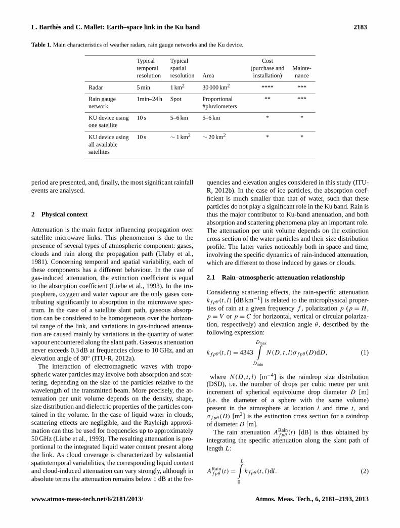
In order to observe rainfall events at an intermediate reso-lution, between that provided by radar and rain gauges, theopportunistic use of these microwave sources was investi-gated based on the use of a low-cost device requiring sig-nificantly less maintenance than a network of rain gauges.A passive ground-based microwave system, capable of es-timating the average rain rate along the Earth–satellite link(hereafter referred to as a “Ku device”), was thus developed.Ground-based power measurements are achieved by receiv-ing Ku-band signals from several operational geostationarysatellites, as was done in the experiments described by Ku-mar et al. (2008), Maitra et al. (2007) and Ramachandran andKumar (2004). The atmospheric attenuation along the Earth–space link are then used to derive the path-averaged rainrates. Table 1 summarizes the main characteristics of weatherradars, rain gauge networks and the Ku device. The proposeddevice is as simple as possible; the final objective is in fact todefine a measurement method that could be easily deployedby using existing dish antennas available everywhere in theworld. In fact, in many parts of the globe, subjected to sig-nificant climatic risk, no operational radar network is avail-able, while microwave systems for television reception are

deployed for a long time. The present paper describes themethod used to retrieve the path-averaged rain rate from Ku-band signals received from geostationary satellites. In an ini-tial step, the measurement principle is described, and the ex-pected accuracy of the Ku-band attenuation measurementsis estimated. A time series of raindrop size distributions isused to estimate the Ku-band attenuation and correspondingrain rate in order to study the influence on attenuation of raininhomogeneity and raindrop size distribution along the linkpath. This section thus provides a relationship between atmo-spheric attenuation and rain rate.

In a second step, the experimental device and the mea-surement campaign designed to test the feasibility of rain-fall measurements using this device are described. Ground-based power measurements were carried out by receivingvarious Ku-band TV channels from different geostationarysatellites. The experimental microwave system was installedclose to Paris during the summer and autumn of 2010. Otherco-located rain observations (rain radar, rain gauges) used forcomparison are also presented.

The third step deals with proposed methods for the re-trieval of rain rates from the received microwave signal, andquantification of the expected rain rate accuracy. In practice,the proposed device measures received power only; however,the reference level of the transmitted signal, relative to whichthe rain attenuation is computed, remains unknown. In thecase of Earth–satellite microwave links, this problem is con-siderably more complex than in the case of point-to-point mi-crowave links, because the measured signal strength dependson several factors, including not only the atmospheric atten-uation resulting from a number of processes such as rain,snow, hail, graupel, water vapour concentration, cloud wa-ter content, turbulence and air temperature, but also the posi-tion of the satellite when viewed from the ground. Most TVsatellites are not in fact perfectly geostationary, since theyhave quasi-circular (slightly elliptic) orbits, which do not lieexactly in the equatorial plane: these are so-called geosyn-chronous orbits which, during the day, induce small relativemovements of the satellite with respect to Earth. These, inturn, lead to small changes in the nominal direction of thetransmitted microwave beam, and therefore to small fluctua-tions in the received signal level (depending on the antennaaperture). In this section a method is proposed for the identi-fication of dry and rainy periods, and for the estimation of thesignal reference level during rainy periods. Finally, by takingthe altitude of the rain into account, the estimated rain atten-uation is retrieved, from which the path-averaged rain ratecan be obtained. The proposed algorithm remains simple be-cause only one channel is used, at a fixed polarization andfrequency; more-sophisticated solutions could be developedin the future by making use of a greater number of channels,at different frequencies and polarizations.

In the last section of this paper, the derived rain rates arecompared with co-located rain gauge and rain radar mea-surements. The statistics obtained from the full experimental

Atmos. Meas. Tech., 6, 2181–2193, 2013 www.atmos-meas-tech.net/6/2181/2013/

L. Barth es and C. Mallet: Earth–space link in the Ku band 2183

Table 1.Main characteristics of weather radars, rain gauge networks and the Ku device.

Typical Typical Costtemporal spatial (purchase and Mainte-resolution resolution Area installation) nance

Radar 5 min 1 km2 30 000 km2 **** ***

Rain gaugenetwork

1min–24 h Spot Proportional#pluviometers

** ***

KU device usingone satellite

10 s 5–6 km 5–6 km * *

KU device usingall availablesatellites

10 s ∼ 1 km2∼ 20 km2 * *

period are presented, and, finally, the most significant rainfallevents are analysed.

2 Physical context

Attenuation is the main factor influencing propagation oversatellite microwave links. This phenomenon is due to thepresence of several types of atmospheric component: gases,clouds and rain along the propagation path (Ulaby et al.,1981). Concerning temporal and spatial variability, each ofthese components has a different behaviour. In the case ofgas-induced attenuation, the extinction coefficient is equalto the absorption coefficient (Liebe et al., 1993). In the tro-posphere, oxygen and water vapour are the only gases con-tributing significantly to absorption in the microwave spec-trum. In the case of a satellite slant path, gaseous absorp-tion can be considered to be homogeneous over the horizon-tal range of the link, and variations in gas-induced attenua-tion are caused mainly by variations in the quantity of watervapour encountered along the slant path. Gaseous attenuationnever exceeds 0.3 dB at frequencies close to 10 GHz, and anelevation angle of 30◦ (ITU-R, 2012a).

The interaction of electromagnetic waves with tropo-spheric water particles may involve both absorption and scat-tering, depending on the size of the particles relative to thewavelength of the transmitted beam. More precisely, the at-tenuation per unit volume depends on the density, shape,size distribution and dielectric properties of the particles con-tained in the volume. In the case of liquid water in clouds,scattering effects are negligible, and the Rayleigh approxi-mation can thus be used for frequencies up to approximately50 GHz (Liebe et al., 1993). The resulting attenuation is pro-portional to the integrated liquid water content present alongthe link. As cloud coverage is characterized by substantialspatiotemporal variabilities, the corresponding liquid contentand cloud-induced attenuation can vary strongly, although inabsolute terms the attenuation remains below 1 dB at the fre-

quencies and elevation angles considered in this study (ITU-R, 2012b). In the case of ice particles, the absorption coef-ficient is much smaller than that of water, such that theseparticles do not play a significant role in the Ku band. Rain isthus the major contributor to Ku-band attenuation, and bothabsorption and scattering phenomena play an important role.The attenuation per unit volume depends on the extinctioncross section of the water particles and their size distributionprofile. The latter varies noticeably both in space and time,involving the specific dynamics of rain-induced attenuation,which are different to those induced by gases or clouds.

2.1 Rain–atmospheric-attenuation relationship

Considering scattering effects, the rain-specific attenuationkfpθ (t, l) [dB km−1] is related to the microphysical proper-ties of rain at a given frequencyf , polarizationp (p = H ,p = V or p = C for horizontal, vertical or circular polariza-tion, respectively) and elevation angleθ , described by thefollowing expression:

kfpθ (t, l) = 4343

Dmax∫Dmin

N(D,t, l)σfpθ (D)dD, (1)

where N(D,t, l) [m−4] is the raindrop size distribution(DSD), i.e. the number of drops per cubic metre per unitincrement of spherical equivolume drop diameterD [m](i.e. the diameter of a sphere with the same volume)present in the atmosphere at locationl and time t , andσfpθ (D) [m2] is the extinction cross section for a raindropof diameterD [m].

The rain attenuationARainfpθ (t) [dB] is thus obtained by

integrating the specific attenuation along the slant path oflengthL:

ARainfpθ (t) =

L∫0

kfpθ (t, l)dl. (2)

www.atmos-meas-tech.net/6/2181/2013/ Atmos. Meas. Tech., 6, 2181–2193, 2013

2184 L. Barthes and C. Mallet: Earth–space link in the Ku band

The extinction cross sectionσfpθ (D) of the raindrops de-pends on the transmitted frequency, the refractive indexn ofthe water, the size and shape of the raindrops, and the polar-ization and incidence angle of the electromagnetic wave. Inthis study,σfpθ (D) is considered to be independent of loca-tion l, even though temperature variations can lead to slightfluctuations in refractive indexn as the drop falls throughthe atmosphere. In the present study, a fixed temperature (setto 10◦C) and negligible induced errors inσfpθ (D) are as-sumed (Atlas and Ulbrich, 1977). Indeed, if the real temper-ature lies in the range 0–20◦C, whereas a fixed temperatureof 10◦C is assumed, the relative specific attenuation error at12 GHz is approximately 2 % when the rain rate is equal to10 mm h−1, and approximately 5.5 % for a rain rate equal to100 mm h−1. Under these conditions, the rain profile alongthe slant path of lengthL can be treated as if it were a sin-gle layer of rain, with an equivalent drop size distributionNe(D, t) [m−4] defined by

Ne(D, t) =1

L

L∫0

N(D,t, l)dl. (3)

The equivalent specific attenuationkfpθ (t) can then beexpressed as

kfpθ (t) = 4343

Dmax∫Dmin

Ne(D, t)σfpθ (D)dD. (4)

The simple relationship describing rain attenuation can bewritten as follows:

ARainfpθ (t) = kfpθ (t)L. (5)

In practice, although the DSD is generally unknown, by con-sidering a gamma drop size distribution, the following em-pirical k–R power law can be used to relate the specific at-tenuation to the rain rate:

kfpθ (t) = afpθ

Rbfpθ (t), (6)

This expression is shown to be an approximation, except inthe low frequency and optical limits (Olsen et al., 1978). Inthe microwave domain,a

fpθandb

fpθdepend on frequency

and to a lesser extent on the drop size distribution, elevationangle and polarization.

2.2 Accuracy of thek–R power law relationship

As shown above, thek–R relation depends on the equiva-lent DSD features, which are the drop concentration and theshape of the DSD. These features depend on the atmosphericconditions (convective or stratiform rain for example) andtheir variability along the radio linkL (i.e. the spatial scaleunder consideration).

Initially, a homogeneous layer with different DSD concen-trations and shapes is considered. As pointed out by Jame-son (1991), thek–R dependence on shape, for a homoge-neous rain layer, is related to frequency. These authors showthat for frequencies close to 25 GHz, this dependence isweak, whereas a stronger dispersion occurs at lower frequen-cies, especially whenf < 9 GHz. In the case of the presentstudy, the use of 12 GHz links could be expected to be moreor less sensitive to the rain microphysics. In order to assessits impact, 1 min drop size distributions were computed fromthe raindrop dataset collected by a disdrometer (Delahaye etal., 2006) over a period of 24 months between July 2008 andJuly 2010. Through the use of an approach similar to thatproposed by Leijnse et al. (2010), for each DSD, the corre-sponding rain rate valueR and specific attenuation valueskfp (Eq. 4) were calculated for 12 GHz using the Mie the-ory (with the drops assumed to be spherical). Under theseconditions, at a temperature equal to 10◦C, the specific at-tenuations are found to be independent of polarization. Fig-ure 1 shows the resulting scatter plot, in which the solid linerepresents the power law fit. For the purposes of compari-son, the dashed curve shows the power law model definedin accordance with the standard International Telecommu-nication Union Recommendation (ref. ITU-R, 2009). It canbe seen that these two curves are very similar, and difficultto distinguish from one another. This figure shows that mi-crophysical discrepancies can lead to an error of±7 mm h−1

in the case of rain rates greater than 10 mm h−1. The rainrate standard deviation varies from 0.2 to 6 mm h−1 whenthe rain rate varies from 1 to 100 mm h−1, with correspond-ing relative standard deviations (RSD) in the range between20 and 6 %. This result shows that 12 GHz is a non-optimalfrequency for the retrieval of low rain rates, and that the pro-posed device would be better adapted to applications involv-ing heavy rainfall events (flash flood forecasting, for exam-ple). The second column of Table 2 shows the coefficients ob-tained by computing linear regressions on the log(k)–log(R)relationship, which are very similar to those given by the ITUmodel (Table 2, columns 7, 8 and 9).

Concerning the variability of the DSD along the radio link,the k–R relationship can be expected to be sensitive to ag-gregation over domains with different volumes. Numerousstudies dealing with radar measurements have investigatedthe Z–R power law relationships (withZ representing thereflectivity andR the rain rate). Morin et al. (2003) have em-pirically shown the existence of a scale dependency of theZ–R law parameters, based on the study of co-located radarand rain gauge data aggregated at different spatial scales.These authors observed a rapid increase in the parametera

as a function of scale, as well as a moderate decrease in theparameterb. Recently, Verrier et al. (2012, 2013) used multi-fractal theory to quantify the impact of rainfall scaling prop-erties on the Z-R relationship. These authors found that whenmultifractal behaviour holds simultaneously forR andZ, the

Atmos. Meas. Tech., 6, 2181–2193, 2013 www.atmos-meas-tech.net/6/2181/2013/

L. Barth es and C. Mallet: Earth–space link in the Ku band 2185

Table 2. Coefficients of linear regression and coefficients of determination obtained by performing linear regressions on log(k) and log(R)scatterplots at a frequencyf equal to 12 GHz and for integration times varying between 1 and 60 min. The last three columns indicate theITU recommendation coefficients corresponding to horizontal, circular and vertical polarizations, respectively, at the same frequency.

1 min 5 min 10 min 30 min 60 min ITU (H) ITU (C) ITU (V)

a 0.027 0.028 0.030 0.030 0.033 0.024 0.024 0.024b 1.15 1.14 1.13 1.12 1.1 1.17 1.15 1.13R2 0.987 0.986 0.98 0.992 0.972 na na na

21

Figures

Fig. 1. Scatter plot of rain rate versus specific attenuation computed from the drop size distribution and Mie theory, for a frequency f equal to 12 GHz and a time resolution of 1 min. The continuous line indicates the corresponding fitted k-R power law. The dotted line indicates the ITU power law for the horizontal polarization.

Fig. 2. Error induced on the rain estimation when the ITU power law is used for an integration time equal to 5 min. For each rain bin, the box-and-whiskers diagram indicates the median (central vertical line), and the lower and upper quartiles (left and right edges of the box). The whiskers indicate the lower and upper limits of the distribution, within 1.5 times the interquartile range, from the lower and upper quartiles, respectively.

0 1 2 3 4 5 60

20

40

60

80

100

120a= 0.027 b= 1.15 Tint = 1 mn R2= 0.987

Rai

n R

ate

(mm

.h-1

)

k (dB.km-1)

Data

FitITU (H)

-12

-10

-8

-6

-4

-2

0

2

4

6

0 10 20 30 40 60 80Rain Rate (mm h-1)

Err

or (

mm

h-1

)

Tint = 5 mn

Fig. 1.Scatter plot of rain rate versus specific attenuation computedfrom the drop size distribution and Mie theory, for a frequencyf

equal to 12 GHz and a time resolution of 1 min. The continuous lineindicates the corresponding fittedk–R power law. The dotted lineindicates the ITU power law for the horizontal polarization.

Z–R relationships can be characterized by{b = constanta ∝ lKR(b) , (7)

whereKR(q) defines the “moment scaling function” of rainof the q-th order, which entirely characterizes the statisticsof the rain field.KR(q) is usually determined by the knowl-edge of a reduced set of “universal” parameters (Schertzerand Lovejoy, 1987). The coefficienta should therefore bea power law of scale, with a scaling exponent that can beshown (from multifractal theory) to be positive whenb > 1,and negative whenb < 1. In order to quantify the impact ofthe scaling properties of rainfall, the study of theZ–R rela-tionship carried out by Verrier et al. (2012, 2013) is applied tothek–R relationships in the present study. Under the assump-tion of a “frozen” atmosphere, an increase in integration timecan be considered as equivalent to the use of larger spatial

scales, and can thus allowk–R relationships to be derived atdifferent spatial scales. The raindrop dataset presented abovewas thus used to compute the DSD with integration timesvarying between 1 and 60 min, from which the correspond-ing k–R relationships were computed. It should be noted thatVerrier et al. (2011) have shown that the rain rate series fol-low multifractal statistics at the mesoscale and the subme-soscale. In Table 2, the stability of the resulting coefficients,associated with the high values of determination coefficient(R2

≥ 0.972), shows that thek–R relationship is rather in-sensitive to integration time, and thus to spatial scale (for thefrequency under consideration). The robustness of thek–R

relationship results from the fact that the exponentb is closeto 1 (1.17), leading to a less critical dependence on scale ofthe parameters in thek–R relationship than of those usedin the Z–R relationships, for whichb is close to 1.6. Morespecifically, in the present case,KR (1.17) is equal to 0.03,whereasKR (1.6) is equal to 0.12 in the case of reflectivityradar. As an example, when integration times of 1 and 10 minare considered, these values lead to a ratio of the prefactora

in thek–R andZ–R relationships respectively equal to 1.07and 1.31. The latter value shows that in the case of a radarsensor, spatial-scale variability can lead to significant errorsunder some meteorological circumstances. Concerning thecoefficientb, Table 2 shows that it remains almost constant(relative error< 3.5 %), as predicted by the theory. The sta-bility of the k–R relationship derived from scale propertiesis relatively well confirmed by the empirical values listed inTable 2, which lie in the range between 1 and approximately30 min, corresponding to spatial scales between a few hun-dred metres and a few km, in accordance with the path lengthL considered in this study. As the estimatedk–R parametersare very close to those provided by the ITU (recommenda-tion: ITU-R, 2009), it was chosen to use these recommendedvalues throughout the remainder of the study. Figure 2 showsthe error statistics determined for specific attenuations, com-puted using Eq. (4), when compared to those obtained usingEq. (6) together with the ITU coefficients. A 5 min integra-tion time was selected to represent a spatial scale compati-ble with the Earth–satellite path lengthL. The correspondingbias lies in the range between 1 and 6 mm h−1, with a relativeerror of less than 10 %.

www.atmos-meas-tech.net/6/2181/2013/ Atmos. Meas. Tech., 6, 2181–2193, 2013

2186 L. Barthes and C. Mallet: Earth–space link in the Ku band

21

Figures

Fig. 1. Scatter plot of rain rate versus specific attenuation computed from the drop size distribution and Mie theory, for a frequency f equal to 12 GHz and a time resolution of 1 min. The continuous line indicates the corresponding fitted k-R power law. The dotted line indicates the ITU power law for the horizontal polarization.

Fig. 2. Error induced on the rain estimation when the ITU power law is used for an integration time equal to 5 min. For each rain bin, the box-and-whiskers diagram indicates the median (central vertical line), and the lower and upper quartiles (left and right edges of the box). The whiskers indicate the lower and upper limits of the distribution, within 1.5 times the interquartile range, from the lower and upper quartiles, respectively.

0 1 2 3 4 5 60

20

40

60

80

100

120a= 0.027 b= 1.15 Tint = 1 mn R2= 0.987

Rai

n R

ate

(mm

.h-1

)

k (dB.km-1)

Data

FitITU (H)

-12

-10

-8

-6

-4

-2

0

2

4

6

0 10 20 30 40 60 80Rain Rate (mm h-1)

Err

or (

mm

h-1

)

Tint = 5 mn

Fig. 2. Error induced on the rain estimation when the ITU powerlaw is used for an integration time equal to 5 min. For each rain bin,the box-and-whiskers diagram indicates the median (central verti-cal line), and the lower and upper quartiles (left and right edges ofthe box). The whiskers indicate the lower and upper limits of thedistribution, within 1.5 times the interquartile range, from the lowerand upper quartiles, respectively.

3 Experimental setup

The experimental system was installed at the LATMOS (Lab-oratoire Atmospheres, Milieux, Observations Spatiales) inGuyancourt, close to Paris, during the summer and autumn of2010. The microwave signals from four geostationary satel-lites (NSS7, AB1, Thor 5/6, and Hot Bird 6/8/9) were re-ceived in horizontal polarization, using a 90 cm diametermultifocus dish antenna. The observed satellite elevationswere close to 30◦. For each satellite, two 30 MHz wide Ku-band channels were received and down-converted to L-bandsignals by four low-noise block converters (LNBC). An RFswitch allowed for sequential selection of one of the L-bandsignals, which was then fed to a field analyser. The latter de-vice has an accuracy of 0.1 dB and is operated in spectrummode, with a 4 MHz bandwidth sequentially centred on eachof the selected channels. The measured signal level was de-termined by averaging five consecutive measurements, andthe averaged value was then stored in a microcomputer usedfor data-logging purposes. The acquisition routine sequen-tially records each of the eight channels, with a 2 s sam-pling period per channel, leading to a total sampling periodequal to 16 s (4 satellites× 2 channels× 2 s). The experi-mental setup is shown in Fig. 3. The frequencies used foreach link are listed in Table 3. It should be noted that in thiscase, the influence of water on the antenna was not taken intoaccount, and will be discussed in Sect. 4.1.

Independent co-located rain observations were also con-sidered in order to evaluate the performance of the proposedKu device: C-band rain rate maps provided by Meteo-France

22

Fig. 3. Experimental setup.

Fig. 4. Locations of the different sites and satellite path links

100 200 300 400 500 600 700 800 900 1000 1100

100

200

300

400

500

600

700

800

Hard disk

RF

Sw

itch

Field Analyser

Coaxial cable (15 m) Micro

Calculator

LNBC

USB

Fig. 3.Experimental setup.

weather radar located at Trappes (close to Guyancourt) andtwo rain gauges, also located at Trappes and Toussus le No-ble, were used. The distances between the LATMOS andthese locations are respectively 2.9 and 3.7 km. Figure 4provides a map of the various sensor locations, as well asthe ground projection of the four Earth–satellite links (bluelines). The dataset can be summarized as follows:

– Eight received signalP chREC(t) time series, with “ch”

ranging from 1 to 8 (4 satellites, each with 2 channels),with a 10 s sampling resolution obtained by applying are-sampling algorithm to the original time series.

– two hourly accumulated rainfall time series,RRG1 (t)andRRG2 (t), obtained with the two rain gauges.

– Twenty thousand radar rain rate mapsRrad(t) with aspatial resolution of 1× 1 km2 and a 5 min temporalresolution. The relationship used to convert radar re-flectivity factors into rain rate was identical to thatused operationally by Meteo-France (Tabary, 2007).The period under consideration includes most of therainfall events which occurred between 23 July and15 December 2010.

In this initial feasibility study, each of the eight availablechannels was used independently. Channel 1 was used to de-velop the algorithms (Sect. 4), such that seven different val-ues of rain rate could then be estimated from the remainingchannels. As these values were found to be quite similar, onlythose obtained with channel 7 are presented in Sect. 5.

Since microwave links provide path-averaged measure-ments, the corresponding average radar path rain rates arecalculated from the rain maps by averaging theRrad

i (t) radarpixels traversed by the link beam, and weighted by the cor-responding length of the linkLi in each pixel.

For each of the eight received channels ch, and each ofthe available radar mapsRrad(t), the average radar rain ratealong the Earth–satellite path can be determined using theradar signals in a given channel by applying the followingexpression:

Rradch (t) =

∑iεI LiR

radi (t)∑

iεI Li

, (8)

where Rradi (t) is the i-th pixel (i∈[1, 262144]) on the

map,I is the subset of pixels intersecting the satellite path

Atmos. Meas. Tech., 6, 2181–2193, 2013 www.atmos-meas-tech.net/6/2181/2013/

L. Barth es and C. Mallet: Earth–space link in the Ku band 2187

Table 3.Frequency [MHz] of the microwave links used in the test campaign.

Channel Satellite Frequency Channel Satellite Frequency (MHz)

1 NSS7 12 604 5 Thor 5/6 12 5632 NSS7 11 694 6 Thor 5/6 12 6883 AB1 12 722 7 Hot Bird 6/8/9 12 2854 AB1 12 547 8 Hot Bird 6/8/9 12 617

22

Fig. 3. Experimental setup.

Fig. 4. Locations of the different sites and satellite path links

100 200 300 400 500 600 700 800 900 1000 1100

100

200

300

400

500

600

700

800

Hard disk

RF

Sw

itch

Field Analyser

Coaxial cable (15 m) Micro

Calculator

LNBC

USB

Fig. 4.Locations of the different sites and satellite path links.

corresponding to channel “ch”, andLi is the length of thelink inside thei-th pixel.

Finally, four time seriesRradch (t) were obtained with a 5 min

temporal resolution, representing the path-averaged rain rateson each Earth–satellite link derived from the radar measure-ments.

In the case of the rain gauges, the two time seriesRRG1(t) and RRG2(t) were simply averaged in order to

obtain RRG2

(t). Figure 5 shows the time seriesP ch1REC(t),

Rradch1(t), RRG(t) for a 10-day period. Each rainy period is

clearly characterized by a temporary fall in received sig-nal strength, revealed by a negative pulse. The precipitationevents can also be seen on the radar and rain gauge time se-ries. It should be noted that the received signals are signifi-cantly affected by daily fluctuations (∼ 1 dB) resulting fromapparent satellite motion and antenna aperture effects, as wellas a negative trend due to a decrease in atmospheric temper-ature and/or water vapour content. For all of these reasons, itis very difficult to directly estimate a reference signal level,from which the rain attenuation can be derived. As explainedin Sect. 4.2, correct estimation of the reference level requiresdry periods to be distinguished from rainy periods, and thisis achieved by analysing the observed fluctuations in signalstrength.

4 Retrieval method

4.1 Reference level

The received signal strength (PREC) expressed by Eq. (8)combines the parameters related to instrumental and geo-metric characteristics, such as the satellite transmitter power(PE), the transmitter and receiver antenna gainsGE, GR,the free-space attenuationAF and the tropospheric attenua-tion (ATrop). Wet antennae can introduce additional attenu-ation effects, depending on the type of antenna (Schleiss etal., 2013; Crane, 2002; Leijnse et al., 2008). To minimizesuch effects, a super hydrophobic coating was applied to thedish and the horn. This type of coating is efficient, and eventhough it does not completely eliminate the presence of allraindrops, the attenuation produced by residual raindrops onthe ground antenna is sufficiently small to be neglected, andthus does not appear in Eq. (8). Moreover in the case ofEarth–space microwave links, only the ground antenna canbecome wet.

PREC(t) = PE(t) + GE(t) + GR(t) − AF(t) − ATrop(t) (dB) (9)

In practice,PE andGE remain almost constant, whereasGRandAF vary slowly over time due to apparent satellite mo-tion. The tropospheric attenuationATrop is critically depen-dent on satellite elevation and the frequency band under con-sideration. In the Ku band, although oxygen (AOxygen), liquidwater in clouds (ACloud), water vapour (Avapour) and scintil-lation (AS) have an influence on signal strength, rain (ARain)

is the dominant contributor to the overall attenuation.

ATrop(t) = AS(t) + AOxygen(t) + ACloud(t)

+AVapour(t) + ARain(t) (dB) (10)

For the purposes of estimating the rain attenuation (ARain),Eq. (8) is expressed as follows:

PREC(t) = PREF(t) − ARain(t) (dB), (11)

wherePPREF(t), which is called the reference level or base-line, is given by

PREF(t) = PE + GE + GR − AF − AS(t)

−AOxygen(t) − ACloud(t) − AVapour(t) (dB). (12)

In the absence of rainfall, we have

PREC(t) = PREF(t) (dB). (13)

www.atmos-meas-tech.net/6/2181/2013/ Atmos. Meas. Tech., 6, 2181–2193, 2013

2188 L. Barthes and C. Mallet: Earth–space link in the Ku band

2.5 3 3.5 4

x 104

-2

-1

0

1

2

3

4

5

6

7

8

Time

Atte

nuat

ion

(dB

)

Rai

n R

ate

(mm

/h)

One day

Fig. 5. Example of recorded time series: received signal (bluecurve), radar rain rate (red curve) and 1 h accumulated rainfall timeseries (dashed green curve).

As the reference level is observed directly during non-rainsituations, during rainfall events its value must be estimatedfrom the reference level obtained during dry periods (Fig. 6),and it is thus essential to develop an algorithm allowing fordry periods to be differentiated from rainy periods. Once thereference level is known, Eqs. (5), (6) and (9) allow for the

corresponding rain rateRKUch (t) to be estimated.

4.2 The rain–no-rain detection algorithm

Each of the atmospheric processes involved has its own dy-namics, and contributes differently to the attenuation of thepropagating electromagnetic wave. As a consequence of itsstrong heterogeneity, rain leads to much more rapid tempo-ral fluctuations of the received signal than gases or clouds.In order to distinguish between dry and rainy periods, an ap-proach similar to those described by Kaufmann and Rieck-ermann (2011) and Schleiss and Berne (2010) is proposed.The various characteristics (trends, standard deviation, kur-tosis, skewness) of the observed Ku-band signal received onchannel 1 were computed using different window sizes cen-tred on current time, and ranging from 100 s to 1 h. The radardata were used to determine the corresponding state of the at-mosphere (rainy or dry). The statistical distributions of theserainy and dry period characteristics were compared in orderto test their ability to discriminate between these two states.The selected window widthW should not be too large, sinceit determines the time delay needed to obtain the estimate.Since the aim of this study is to develop a sensor allowingfor near-real-time observations to be made, the time windowswere chosen to be as small as possible, whilst ensuring gooddiscrimination.

Two characteristics were selected (see Eq. 10): the stan-dard deviation for a 30 min time window, and the local trend

Fig. 6. Received signal during a rain event

Dry period Dry period Rainy period

Reference level Estimated Reference level

Rain attenuation Ap(t)

Fig. 6.Received signal during a rain event.

over a 4 min time window.

std(PREC(n)) =

[1

2W+1

L∑i=−L

(PREC(n + i) − PREC(n))2

]12

with P REC(n)= 12W+1

L∑i=−L

PREC(n + i) and W=100

Trd(PREC(n)) =1W

L∑i=−L

aiPREC(n + i)

with a = (−1,−1, . . . − 1,0,1, . . .1) and W=10

(14)

The aim of this approach was to develop a pattern classifier,providing an appropriate rule for the assignment of each sam-plePREC(n) into one of the two classes (rainy or dry). Sincethe optimal boundary between the two regions, referred to asa decision boundary, is non-linear, it was considered prefer-able to make use of an artificial neural network. The so-calledmulti-layer perceptron (MLP) algorithm used here, whichis able to learn complex (non-linear) and multi-dimensionalmapping from a collection of examples, is an ideal classifier(Haykin, 1999); the MLP is defined by its topology, namelythe dimensions of the input and output vectors and the num-ber of hidden neurons, and by its weights. A training pro-cess is needed to determine the optimal weights. This stepis called the training process, and requires a representativedatabase comprising a wide set of input and output vectors(Xn,Y n):

Xn= [std(PREC(n)),Trd(PREC(n))]

Y n=

0 if R

radch1(n) < 0.1 mmh−1

belongstoadryperiod

1 if Rradch1(n) > 0.1 mmh−1

belongstoarainyperiod.

(15)

The training database comprises half of the dataset measuredby channel 1 (1 336 201 samples), whereas the other half isused to determine the optimal architecture (six hidden neu-rons) in terms of generalization ability. The generalizationproperty makes it possible to train an MLP with a repre-sentative set of input/target pairs, and to obtain good resultswhen predicting unseen input samples. Following training,the MLP output provides a direct estimation of the posteriorprobabilities (Zhang, 2000), as shown in Fig. 7a.

Once it has been determined, the MLP can be applied tothe entire dataset for the purposes of identifying dry and rainy

Atmos. Meas. Tech., 6, 2181–2193, 2013 www.atmos-meas-tech.net/6/2181/2013/

L. Barth es and C. Mallet: Earth–space link in the Ku band 2189

Fig. 7. (a)MLP output: posterior rain class probability.(b) Bound-ary of the classifier (green solid line), samples corresponding to thedry class are in blue, and samples corresponding to the rainy classare in red.

episodes. The discriminating rule is simple: assign samplen

to the rainy class ifY n≥ Po, or to the dry class ifY n < Po.

Figure 7b provides a plot of the boundary (solid line) be-tween the two classes. The determination ofPo is describedin detail below.

Following the identification of dry and rainy periods basedon MLP analysis of the received signals, the reference levelis interpolated during rainy periods, allowing for the rain at-tenuationARain(t) to be estimated. Using Eq. (12) to expressthe geometric path lengthL (ITU-R, 2009), the specific at-tenuationkfpθ (t) can be estimated using Eq. (5).

L =hR−hSsin(θ)

hR = h0 + 0.36(km),(16)

wherehR is the altitude of the top of the layer of rain andh0 isthe annual average altitude above mean sea level of the 0◦Cisotherm. According to the ITU-R (2001) recommendation,the latter parameter can be taken to be 3 km in the presentcase. The parameterhS is the altitude of the ground stationandθ is the elevation angle. Finally, the corresponding rain

rateRKUch1(t) is given by Eq. (6). The probability thresholdPo

(determined as 0.55) is chosen so that the CDF corresponding

to the 1 h accumulatedRKUch1(t) is as close as possible to that

of RKUch1(t) (see Fig. 8). It should be noted that this thresh-

old gives a percentage of rain similar to that obtained overthe same period with a disdrometer, located 10 km from thereceiver, when a 0.1 mm h−1 threshold is applied.

5 Validation and results

The method described in the preceding sections was used to

estimateRKUch7(t). A characteristics vectorX, corresponding

to channel 7, was computed from the time seriesP ch7REC(t)

and then applied to the MLP, with which the threshold Po

was used to discriminate between rainy and dry periods. Inorder to quantify the performance of the device and associ-

ated algorithm, comparisons were then made withRradch7(t)

andRRG

(t) using different criteria. Firstly, the rainfall inten-

24

Fig. 8. Percentage of rain vs 1-hour accumulated rain threshold for the radar time series (green), rain gauges (red), and KU device (blue), for a threshold Po = 0.55.

Fig. 9. Examples of time series recorded by the Ku device (red curve) and the radar (blue curve).

0 2 4 6 8 10 120

1

2

3

4

5

6

7

Threshold (mm)

Per

cent

age

of r

ain

(%)

Ku

RadPluvio

16:48 18:00 19:12 20:24 21:36 22:480

2

4

6

8

10

12

14

16

18

20

Time

Rai

n ra

te (

mm

/h)

Fig. 8.Percentage of rain vs. 1 h accumulated rain threshold for theradar time series (green), rain gauges (red) and KU device (blue) fora thresholdPo = 0.55.

24

Fig. 8. Percentage of rain vs 1-hour accumulated rain threshold for the radar time series (green), rain gauges (red), and KU device (blue), for a threshold Po = 0.55.

Fig. 9. Examples of time series recorded by the Ku device (red curve) and the radar (blue curve).

0 2 4 6 8 10 120

1

2

3

4

5

6

7

Threshold (mm)

Per

cent

age

of r

ain

(%)

Ku

RadPluvio

16:48 18:00 19:12 20:24 21:36 22:480

2

4

6

8

10

12

14

16

18

20

Time

Rai

n ra

te (

mm

/h)

Fig. 9. Examples of time series recorded by the Ku device (redcurve) and the radar (blue curve).

sity time series measured by the rain radar and determinedwith the Ku device were compared visually. The order ofmagnitude and dynamics of the two measurements can beseen to be similar (Fig. 9), even though these two quantitiescannot be rigorously equal as a consequence of the differentsampling volumes, altitudes and time resolutions involved inthese two sets of data. Figure 10 compares the accumulatedrainfall recorded by the gauges and rain radar, with the valuesestimated from the received signals over a 4 month period.The same accumulated rainfall, i.e. a total height of 220 mm,is determined by the radar and the Ku device, whereas therain gauges record a slightly higher value.

Figure 11 provides a comparison between the hourly ac-cumulated rainfall measured by the radar and the Ku device(top), and between the rain gauge and the Ku device (bot-tom). The quantile–quantile plots (left-hand side of the fig-ure) are relatively close to the diagonal, showing that the 1 haccumulated rainfall distributions are quite similar. Error boxplots are provided on the right-hand side of this figure. Themedian values are close to zero, especially in the case of the

www.atmos-meas-tech.net/6/2181/2013/ Atmos. Meas. Tech., 6, 2181–2193, 2013

2190 L. Barthes and C. Mallet: Earth–space link in the Ku band

25

Fig. 10. Accumulated rainfall determined using the radar data (blue curve), rain gauge (green curve) and Ku-

band attenuation measurements (red curve), over a 4 month period..

0 20 40 60 80 100 1200

50

100

150

200

250

Time (Days)

Acc

umul

ated

rai

nfal

l (m

m)

Radar

KuPluv

Fig. 10.Accumulated rainfall determined using the radar data (bluecurve), rain gauge (green curve) and Ku-band attenuation measure-ments (red curve) over a 4 month period.

comparison between the Ku device and the radar, with theexception of the intermediate value of accumulated rainfall(−1.3 mm). In the case of both box plots, it can be seen thatthe width of the boxes, defined as the separation between the25th and 75th percentiles, increases when the accumulatedrainfall increases. Several explanations are proposed for thisphenomenon in the following paragraph.

Rainfall event case studies

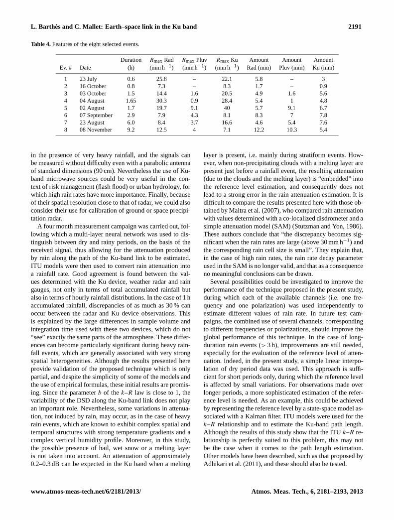
Eight rainfall events of various intensities and durations wereselected. Although these cannot be considered to be repre-sentative of the local rainfall climatology, they nonethelessmake it possible to highlight several features of the Ku-bandrainfall data. The dates, durations, maximum rain rates andquantities of rain estimated by the radar, the rain gaugesand the Ku device are provided in Table 4. The events aresorted by increasing duration. Note that the maximum rainratesRmax are obtained with different integration times, de-pending on the type of measurement (rain gauges: 1 h, rainradar: 5 min, Ku device 1 s). It can be seen that the quantitiesof rain estimated by the radar and the Ku-band sensor arerelatively close to each other (deviation< 15 %) for eventslasting between 1 and 3 hours (events 3, 4, 5 and 6). How-ever, this is not the case for very brief (< 1 h) events, nor forlong rainfall events (> 6 h). In the case of the short-durationevents (events 1 and 2), the maximum values ofRmax for therain radar and Ku device are relatively close to each other,although it is difficult to compare the measured quantities ofrain as a consequence of the small size of the rain cells. In-deed, in the case of small rain cells traversed more or lessperpendicularly by the microwave link, the cell is observedfor only a few seconds or minutes, whereas it is observed fora longer period of time in the corresponding rain radar pixel,since the latter are much greater in size (1 km) than those cor-responding to the microwave link (a few metres). Thus, thetwo instruments may not necessarily have observed exactly

26

Fig. 11. Q-Q plots using radar and Ku device data (top left), and rain gauge and Ku device data (bottom left). Box plots made using radar and Ku device data (top right), and rain gauge and Ku device data (bottom right).

-4

-2

0

2

4

0 1 2 3 4 61-hour radar cumulated rainfall (mm)

Err

or (

mm

)

-4

-2

0

2

4

0 1 2 3 4 5 6 91-hour pluviometer cumulated rainfall (mm)

Err

or (

mm

)

0 2 4 6 8 100

2

4

6

8

10

1-hour Cumulated Ku device rainfall (mm)

1-ho

ur C

umul

ated

rad

ar r

ainf

all

(mm

)

0 2 4 6 8 100

2

4

6

8

10

1-hour Cumulated Ku device rainfall (mm)

1-ho

ur C

umul

ated

plu

viom

eter

rai

nfal

l (m

m))

Fig. 11. Q–Q plots using radar and Ku device data (top left), andrain gauge and Ku device data (bottom left). Box plots made usingradar and Ku device data (top right), and rain gauge and Ku devicedata (bottom right).

the same phenomena. In the case of long-duration rainfallevents (events 7 and 8), the reason for the discrepancy in theobservations is completely different. The simple interpola-tion technique used to calculate the reference level appearsto have been unsuitable because of daily variations of refer-ence level, and a more sophisticated method should be usedin the future. It should be noted that in all cases, there areseveral reasons for which it is difficult to compare the re-sults obtained with these two devices: (i) it is well knownthat the radarZ–R equation sometimes overestimates or un-derestimates the rain rate, (ii) the path lengthL can be under-or over-estimated if the 0◦ isotherm is not sufficiently wellknown, and (iii) in the presence of high rainfall rates, associ-ated with very strong spatial heterogeneities, significant dif-ferences can occur because the instruments do not see thesame volume of the atmosphere.

6 Conclusions

Ku-band microwave sources on geostationary satellites, suchas those used in telecommunications or broadcasting, can po-tentially be used for the estimation of rainfall. A low-cost,ground-based microwave system allowing for atmosphericattenuation to be estimated along Earth–satellite links wasdeveloped in order to investigate the opportunistic use ofthese microwave sources in the frequency band between 10.7and 12.7 GHz. Although this band is not optimal for the esti-mation of weak rainfall rates, due to its lack of sensitivity, itappears to be a good choice when the rainfall rate increases,since in this case the attenuation rarely exceeds 12 dB, even

Atmos. Meas. Tech., 6, 2181–2193, 2013 www.atmos-meas-tech.net/6/2181/2013/

L. Barth es and C. Mallet: Earth–space link in the Ku band 2191

Table 4.Features of the eight selected events.

Duration Rmax Rad Rmax Pluv Rmax Ku Amount Amount AmountEv. # Date (h) (mm h−1) (mm h−1) (mm h−1) Rad (mm) Pluv (mm) Ku (mm)

1 23 July 0.6 25.8 – 22.1 5.8 – 32 16 October 0.8 7.3 – 8.3 1.7 – 0.93 03 October 1.5 14.4 1.6 20.5 4.9 1.6 5.64 04 August 1.65 30.3 0.9 28.4 5.4 1 4.85 02 August 1.7 19.7 9.1 40 5.7 9.1 6.76 07 September 2.9 7.9 4.3 8.1 8.3 7 7.87 23 August 6.0 8.4 3.7 16.6 4.6 5.4 7.68 08 November 9.2 12.5 4 7.1 12.2 10.3 5.4

in the presence of very heavy rainfall, and the signals canbe measured without difficulty even with a parabolic antennaof standard dimensions (90 cm). Nevertheless the use of Ku-band microwave sources could be very useful in the con-text of risk management (flash flood) or urban hydrology, forwhich high rain rates have more importance. Finally, becauseof their spatial resolution close to that of radar, we could alsoconsider their use for calibration of ground or space precipi-tation radar.

A four month measurement campaign was carried out, fol-lowing which a multi-layer neural network was used to dis-tinguish between dry and rainy periods, on the basis of thereceived signal, thus allowing for the attenuation producedby rain along the path of the Ku-band link to be estimated.ITU models were then used to convert rain attenuation intoa rainfall rate. Good agreement is found between the val-ues determined with the Ku device, weather radar and raingauges, not only in terms of total accumulated rainfall butalso in terms of hourly rainfall distributions. In the case of 1 haccumulated rainfall, discrepancies of as much as 30 % canoccur between the radar and Ku device observations. Thisis explained by the large differences in sample volume andintegration time used with these two devices, which do not“see” exactly the same parts of the atmosphere. These differ-ences can become particularly significant during heavy rain-fall events, which are generally associated with very strongspatial heterogeneities. Although the results presented hereprovide validation of the proposed technique which is onlypartial, and despite the simplicity of some of the models andthe use of empirical formulas, these initial results are promis-ing. Since the parameterb of thek–R law is close to 1, thevariability of the DSD along the Ku-band link does not playan important role. Nevertheless, some variations in attenua-tion, not induced by rain, may occur, as in the case of heavyrain events, which are known to exhibit complex spatial andtemporal structures with strong temperature gradients and acomplex vertical humidity profile. Moreover, in this study,the possible presence of hail, wet snow or a melting layeris not taken into account. An attenuation of approximately0.2–0.3 dB can be expected in the Ku band when a melting

layer is present, i.e. mainly during stratiform events. How-ever, when non-precipitating clouds with a melting layer arepresent just before a rainfall event, the resulting attenuation(due to the clouds and the melting layer) is “embedded” intothe reference level estimation, and consequently does notlead to a strong error in the rain attenuation estimation. It isdifficult to compare the results presented here with those ob-tained by Maitra et al. (2007), who compared rain attenuationwith values determined with a co-localized disdrometer and asimple attenuation model (SAM) (Stutzman and Yon, 1986).These authors conclude that “the discrepancy becomes sig-nificant when the rain rates are large (above 30 mm h−1) andthe corresponding rain cell size is small”. They explain that,in the case of high rain rates, the rain rate decay parameterused in the SAM is no longer valid, and that as a consequenceno meaningful conclusions can be drawn.

Several possibilities could be investigated to improve theperformance of the technique proposed in the present study,during which each of the available channels (i.e. one fre-quency and one polarization) was used independently toestimate different values of rain rate. In future test cam-paigns, the combined use of several channels, correspondingto different frequencies or polarizations, should improve theglobal performance of this technique. In the case of long-duration rain events (> 3 h), improvements are still needed,especially for the evaluation of the reference level of atten-uation. Indeed, in the present study, a simple linear interpo-lation of dry period data was used. This approach is suffi-cient for short periods only, during which the reference levelis affected by small variations. For observations made overlonger periods, a more sophisticated estimation of the refer-ence level is needed. As an example, this could be achievedby representing the reference level by a state-space model as-sociated with a Kalman filter. ITU models were used for thek–R relationship and to estimate the Ku-band path length.Although the results of this study show that the ITUk–R re-lationship is perfectly suited to this problem, this may notbe the case when it comes to the path length estimation.Other models have been described, such as that proposed byAdhikari et al. (2011), and these should also be tested.

www.atmos-meas-tech.net/6/2181/2013/ Atmos. Meas. Tech., 6, 2181–2193, 2013

2192 L. Barthes and C. Mallet: Earth–space link in the Ku band

The present study deals with the estimation of rainfallrate, using Ku-band attenuation over a single path link. Inthe future, the use of several simultaneous links associatedwith tomography or assimilation methods, based on an ap-proach similar to that of Zinevich et al. (2008, 2009) orGiulli et al. (1997, 1999), could be applied to the estima-tion of small-scale rainfall fields, and could be helpful in hy-drological applications, flash flood forecasting and weatherradar calibration.

Acknowledgements.This work was supported by theFrench “Programme National de Teledetection Spa-tiale” (PNTS, http://www.insu.cnrs.fr/actions-sur-projets/pnts-programme-national-de-teledetection-spatiale), grantno. PNTS-2013-01. The authors would like to thank M. Parent duChatelet from Meteo-France for various fruitful discussions on thetopic of radar data processing.

Edited by: F. S. Marzano

References

Adhikari, A., Das, S., Bhattacharya, A., and Maitra, A.: Improvingrain attenuation estimation: modelling of effective path lengthusing ku-band measurements at a tropical location, Prog. Elec-tromagn. Res. B, 34, 173–186, 2011.

Atlas, D. and Ulbrich, C. W.: Path- and Area-Integrated RainfallMeasurement by Microwave Attenuation in the 1–3 cm Band, J.Appl. Meteor., 16, 1322–1331, 1977.

Berne, A. and Uijlenhoet, R.: Path-averaged rainfall esti-mation using microwave links: Uncertainty due to spa-tial rainfall variability, Geophys. Res. Lett., 34, L07403,doi:10.1029/2007GL029409, 2007.

Crane, R. K.: Analysis of the effects of water on the ACTS propa-gation terminal antenna, Antennas and Propagation, IEEE Trans.,50, 954–965, 2002.

Delahaye, J. Y., Barthes, L., Gole, P., Lavergnat, J., and Vinson,J. P.: a dual beam spectropluviometer concept, J. Hydrol., 328,110–120, 2006.

Fenicia, F., Pfister, L., Kavetski,D., Matgen, P., Iffly, J. F., Hoff-mann, L., and Uijlenhoet, R.: Microwave links for rainfall esti-mation in an urban environment: Insights from an experimentalsetup in Luxembourg-City, J. Hydrol., 464–465, 69–78, 2012.

Giuli, D., Facheris, L., and Tanelli, S.: A new microwave tomog-raphy approach for rainfall monitoring over limited areas, Phys.Chem. Earth, 22, 265–273, 1997.

Giuli, D., Facheris, L., and Tanelli, S.: Microwave tomographic in-version technique based on stochastic approach for rainfall fieldsmonitoring, IEEE T. Geosci. Remote, 37, 2536–2555, 1999.

Haykin, S.: Neural Networks: comprehensive Foundation, Prentice-Hall, Upper Saddle River, N.J., 1999.

ITU-R: Propagation data and prediction methods required forthe design of terrestrial line-of-sight systems: RecommendationITU-R P.530 -9, 2001.

ITU-R: Propagation data and prediction methods required forearthspace telecommunication systems: Recommendation ITU-R P.618-9, ITU-R Recommendations, P-Series Fascicle, ITU,Geneva, 2009.

ITU-R: Attenuation by atmospheric gases, Recommendation ITU-R P.676-9, available at:www.itu.int/rec/R-REC-P.676(last ac-cess: 28 August 2013), 2012a.

ITU-R: Attenuation due to clouds and fog, Recommendation ITU-R P.840-5, available at:www.itu.int/rec/R-REC-P.840(last ac-cess: 28 August 2013), 2012b.

Jameson, A. R.: A Comparison of Microwave Techniques for Mea-suring Rainfall. J. Appl. Meteor., 30, 32–54, 1991.

Kaufmann, M. and Rieckermann, J.: Identification of dryand rainy periods using telecommunication microwavelinks, 12nd International Conference on Urban Drainage,Porto Alegre/Brazil, 10–15 September, 2011, availableat: http://www.yumpu.com/en/document/view/6346597/identification-of-dry-and-rainy-periods-using-telecommunication-,2011.

Kumar, S., Bhaskara, V., and Narayana Rao, D.: Prediction of KuBand Rain Attenuation Using Experimental Data and Simula-tions for Hassan, India, Int. J. Comput. Sci. Netw. Sec., 8, 10–15,2008.

Leijnse, H., Uijlenhoet, R., and Stricker, J. N. M.: Rainfall measure-ment using radio links from cellular communication networks,Water Resour. Res., 43, W03201, doi:10.1029/2006WR005631,2007.

Leijnse, H., Uijlenhoet, R., and Stricker, J. N. M.: Microwave linkrainfall estimation: Effects of link length and frequency, temporalsampling, power resolution, and wet antenna attenuation, Adv.Water Resour., 31, 1481–1493, 2008.

Leijnse, H., Uijlenhoet, R., and Berne, A.: Errors and Uncertain-ties in Microwave Link Rainfall Estimation Explored Using DropSize Measurements and High-Resolution Radar Data, J. Hy-drometeor., 11, 1330–1344, 2010.

Liebe, H. J., Hufford, G. A., and Cotton, M. G.: Propagation Mod-eling of Moist Air and Suspended Water/Ice Particles at Frequen-cies below 1000 GHz, AGARD Conference, Atmospheric Prop-agation Effects through Natural and Man-Made Obscurants forVisible to MM-Wave Radiation, 542, 3.1–3.10, 1993.

Maitra, A., Kaustav, C., Sheershendu, B., and Srijibendu, B.: Prop-agation studies at Ku-band over an earth-space path at Kolkata,Ind. J. Radio Sp. Phys., 36, 363–368, 2007.

Messer, H., Zinevich, A., and Alpert, P.: Environmental monitoringby wireless communication networks, Science, 312, 713–716,2006.

Morin, E., Krajewski, W. F., Goodrich, D., Xiaogang, G., andSorooshian S.: Estimating rainfall intensities from weather radardata: the scale-dependency problem, J. Hydromet., 4, 782–797,2003.

Olsen, R. L., Rogers, D. V., and Hodge, D. B .: The aRb relationin the calculation of the rain attenuation, IEEE Trans. AntennasPropag., 26, 318–329, 1978.

Overeem, A., Leijnse, H., and Uijlenhoet, R.: Country-wide rainfallmaps from cellular communication networks, Proc. Natl. Acad.Sci., 110, 2741–2745, doi:10.1073/pnas.1217961110, 2013.

Ramachandran, V. and Kumar, V.: Rain Attenuation Measurementon Ku-band Satellite TV Downlink in Small Island, Electron.Lett., 40, 49–50, 2004.

Atmos. Meas. Tech., 6, 2181–2193, 2013 www.atmos-meas-tech.net/6/2181/2013/

L. Barth es and C. Mallet: Earth–space link in the Ku band 2193

Schertzer, D. and Lovejoy, S.: Physically based rain and cloud mod-eling by anisotropic, multiplicative turbulent cascades, J. Geo-phys. Res., 92, 9692–9714, 1987.

Schleiss, M. and Berne, A.: Identification of dry and rainy peri-ods using telecommunciation microwave links, IEEE Geosci. Re-mote Sens. Lett., 7, 611–615, 2010.

Schleiss, M., Rieckermann, J., and Berne, A.: Quantificationand modeling of wet-antenna attenuation for commercial mi-crowave links, IEEE Geosci. Remote Sens. Lett., PP (99),doi:10.1109/LGRS.2012.2236074, 2013.

Stutzman, W. L. and Yon, K. M.: A simple rain attenuation modelfor earth-space radio links operating at 10–35 GHz, Radio Sci.,21, 65–72, doi:10.1029/RS021i001p00065, 1986.

Tabary, P.: The new french operational radar rainfall product. Part I:methodology, Weather Forecast., 22, 393–408, 2007.

Ulaby, F. T., Moore, R. K., and Fung, A. K.: Microwave RemoteSensing, Active and Passive, Vol. 1, Microwave Remote SensingFundamentals and Radiometry, Artech house Inc., 1981.

Upton, G. J. G., Holt, A. R., Cummings, R. J., Rahimi, A. R., andGoddard, J. W. F.: microwave links: the future for urban rainfallmeasurement?, Atmos. Res., 77, 300–312, 2005.

Verrier, S., Mallet, C., and Barthes, L.: Multiscaling properties ofrain in the time domain, taking into account rain support biases, J.Geophys. Res., 116, D20119, doi:10.1029/2011JD015719, 2011.

Verrier, S., Barthes, L., and Mallet, C.: Scaling properties of rainfallin space and time and their impact on rain rate estimation fromweather radar 7th European Conference on Radar in Meteorol-ogy and Hydrology ERAD2012, Toulouse France, 2012.

Verrier, S., Barthes L., and Mallet C.: Theoretical and em-pirical scale-dependency of Z-R relationships: evidence, im-pacts and correction, J. Geophys. Res., 118, 7435–7449,doi:10.1002/jgrd.v118.14, 2013.

Wang, Z., Schleiss, M., Jaffrain, J., Berne, A., and Rieckermann, J.:Using Markov switching models to infer dry and rainy periodsfrom telecommunication microwave link signals, Atmos. Meas.Tech., 5, 1847–1859, doi:10.5194/amt-5-1847-2012, 2012.

Zhang, G. P.: Neural Networks for Classification: A Survey, IEEETrans. Syst., Man, Cybern., Part C: applications and reviews, 30,451–462, 2000.

Zinevich, A., Alpert, P., and Messer, H.: Estimation of rainfall fieldsusing commercial microwave communication networks of vari-able density, A. Water Res., 31, 1470–1480, 2008.

Zinevich, A., Messer, H., and Alpert, P.: Frontal Rainfall Observa-tion by a Commercial Microwave Communication Network, J.Appl. Meteor. Climatol., 48, 1317–1334, 2009.

www.atmos-meas-tech.net/6/2181/2013/ Atmos. Meas. Tech., 6, 2181–2193, 2013