hpc best practices for fea - ansys · 1 © 2012 ansys, inc. may 18, 2012 . hpc best practices for...
TRANSCRIPT

© 2012 ANSYS, Inc. May 18, 2012 1
HPC Best Practices for FEA
John Higgins, PE
Senior Application Engineer
© 2012 ANSYS, Inc. May 18, 2012 2
Agenda
• Overview
• Parallel Processing Methods
• Solver Types
• Performance Review
• Memory Settings
• GPU Technology
• Software Considerations
• Appendix
© 2012 ANSYS, Inc. May 18, 2012 3
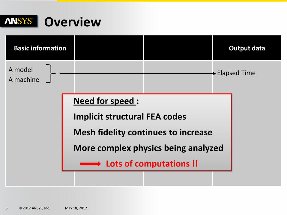
Basic information Output data
A model
A machine Elapsed Time
Overview
Need for speed :
Implicit structural FEA codes
Mesh fidelity continues to increase
More complex physics being analyzed
Lots of computations !!
© 2012 ANSYS, Inc. May 18, 2012 4
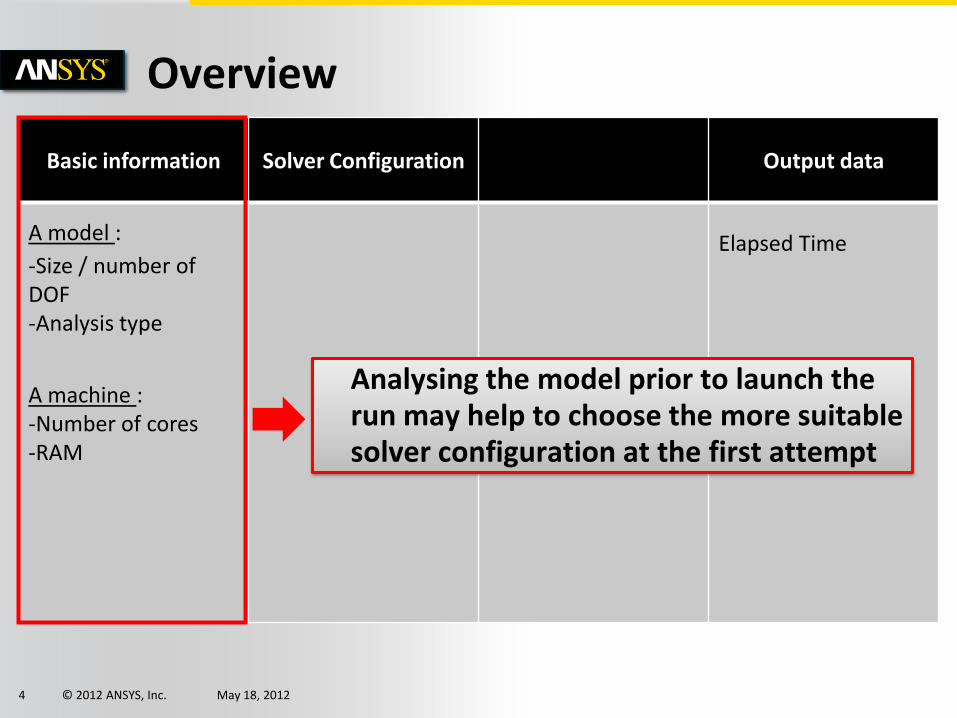
Basic information Solver Configuration Output data
A model :
-Size / number of DOF -Analysis type
A machine : -Number of cores -RAM
Elapsed Time
Overview
Analysing the model prior to launch the run may help to choose the more suitable solver configuration at the first attempt
© 2012 ANSYS, Inc. May 18, 2012 5
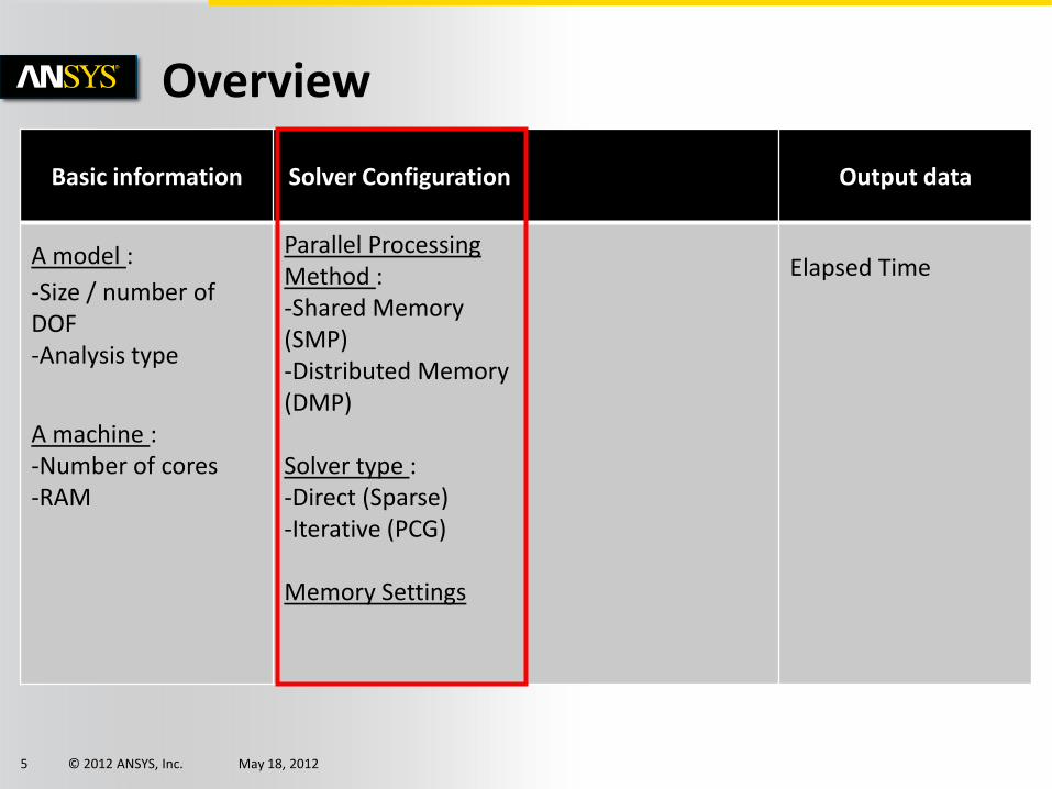
Basic information Solver Configuration Output data
A model :
-Size / number of DOF -Analysis type
A machine : -Number of cores -RAM
Parallel Processing Method : -Shared Memory (SMP) -Distributed Memory (DMP)
Solver type : -Direct (Sparse) -Iterative (PCG)
Memory Settings
Elapsed Time
Overview
© 2012 ANSYS, Inc. May 18, 2012 6
Basic information Solver Configuration Information during
the solve Output data
A model :
-Size / number of DOF -Analysis type
A machine : -Number of cores -RAM
Parallel Processing Method : -Shared Memory (SMP) -Distributed Memory (DMP)
Solver type : -Direct (Sparse) -Iterative (PCG)
Memory Settings
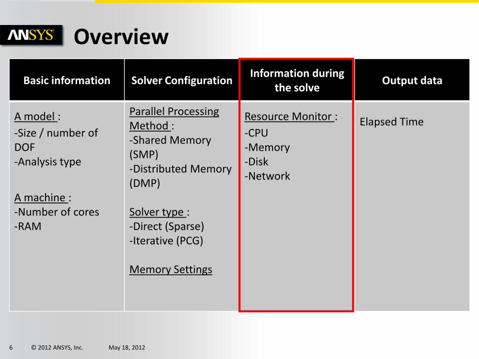
Resource Monitor :
-CPU -Memory -Disk -Network
Elapsed Time
Overview
© 2012 ANSYS, Inc. May 18, 2012 7
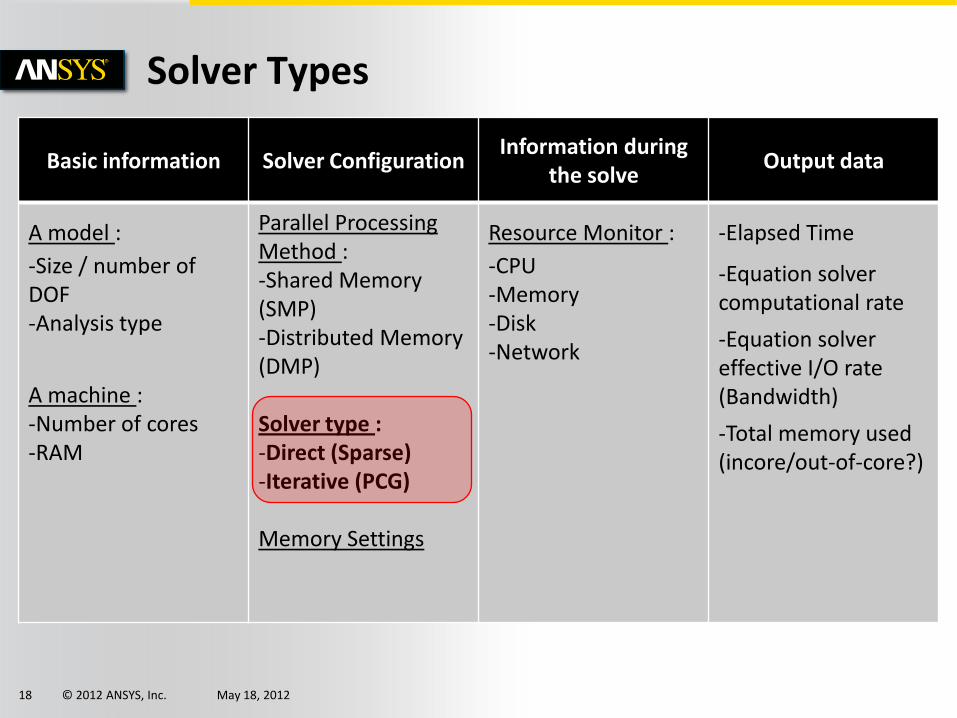
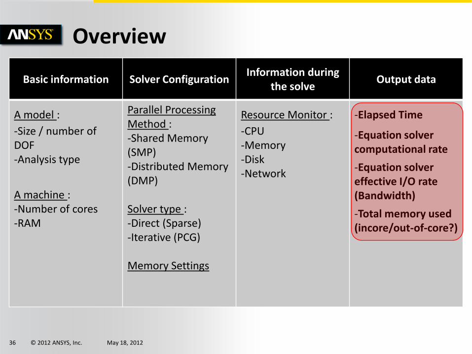
Basic information Solver Configuration Information during
the solve Output data
A model :
-Size / number of DOF -Analysis type
A machine : -Number of cores -RAM
Parallel Processing Method : -Shared Memory (SMP) -Distributed Memory (DMP)
Solver type : -Direct (Sparse) -Iterative (PCG)
Memory Settings
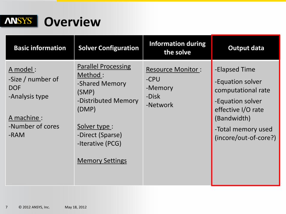
Resource Monitor :
-CPU -Memory -Disk -Network
-Elapsed Time
-Equation solver computational rate
-Equation solver effective I/O rate (Bandwidth)
-Total memory used (incore/out-of-core?)
Overview
© 2012 ANSYS, Inc. May 18, 2012 8
Basic information Solver Configuration Information during
the solve Output data
A model :
-Size / number of DOF -Analysis type
A machine : -Number of cores -RAM
Parallel Processing Method : -Shared Memory (SMP) -Distributed Memory (DMP)
Solver type : -Direct (Sparse) -Iterative (PCG)
Memory Settings
Resource Monitor :
-CPU -Memory -Disk -Network
-Elapsed Time
-Equation solver computational rate
-Equation solver effective I/O rate (Bandwidth)
-Total memory used (incore/out-of-core?)
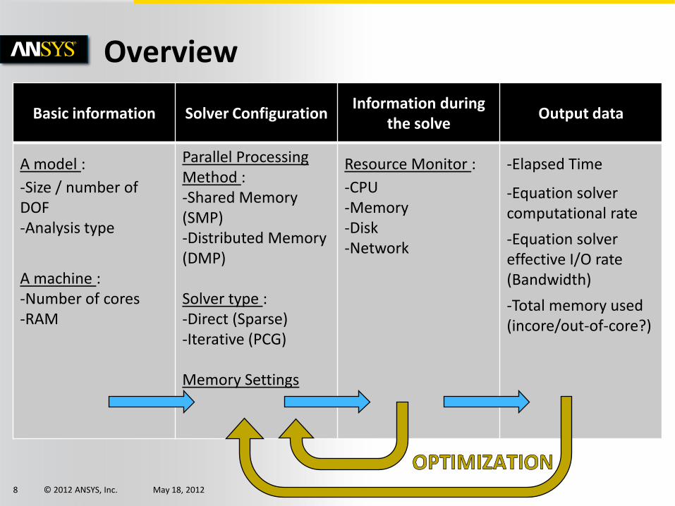
Overview
© 2012 ANSYS, Inc. May 18, 2012 9
Basic information Solver Configuration Information during
the solve Output data
A model :
-Size / number of DOF -Analysis type
A machine : -Number of cores -RAM
Parallel Processing Method : -Shared Memory (SMP) -Distributed Memory (DMP)
Solver type : -Direct (Sparse) -Iterative (PCG)
Memory Settings
Resource Monitor :
-CPU -Memory -Disk -Network
-Elapsed Time
-Equation solver computational rate
-Equation solver effective I/O rate (Bandwidth)
-Total memory used (incore/out-of-core?)
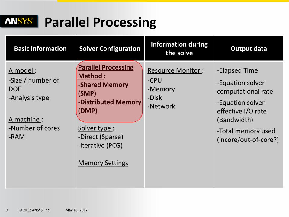
Parallel Processing
© 2012 ANSYS, Inc. May 18, 2012 10
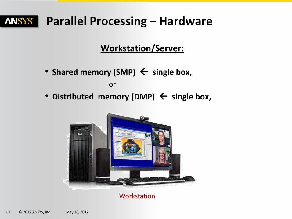
Workstation/Server:
• Shared memory (SMP) single box,
or
• Distributed memory (DMP) single box,
Parallel Processing – Hardware
Workstation
© 2012 ANSYS, Inc. May 18, 2012 11
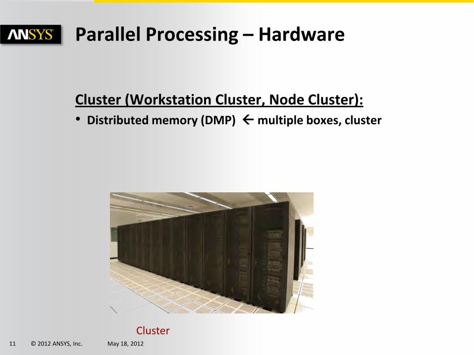
Cluster (Workstation Cluster, Node Cluster):
• Distributed memory (DMP) multiple boxes, cluster
Parallel Processing – Hardware
Cluster
© 2012 ANSYS, Inc. May 18, 2012 12
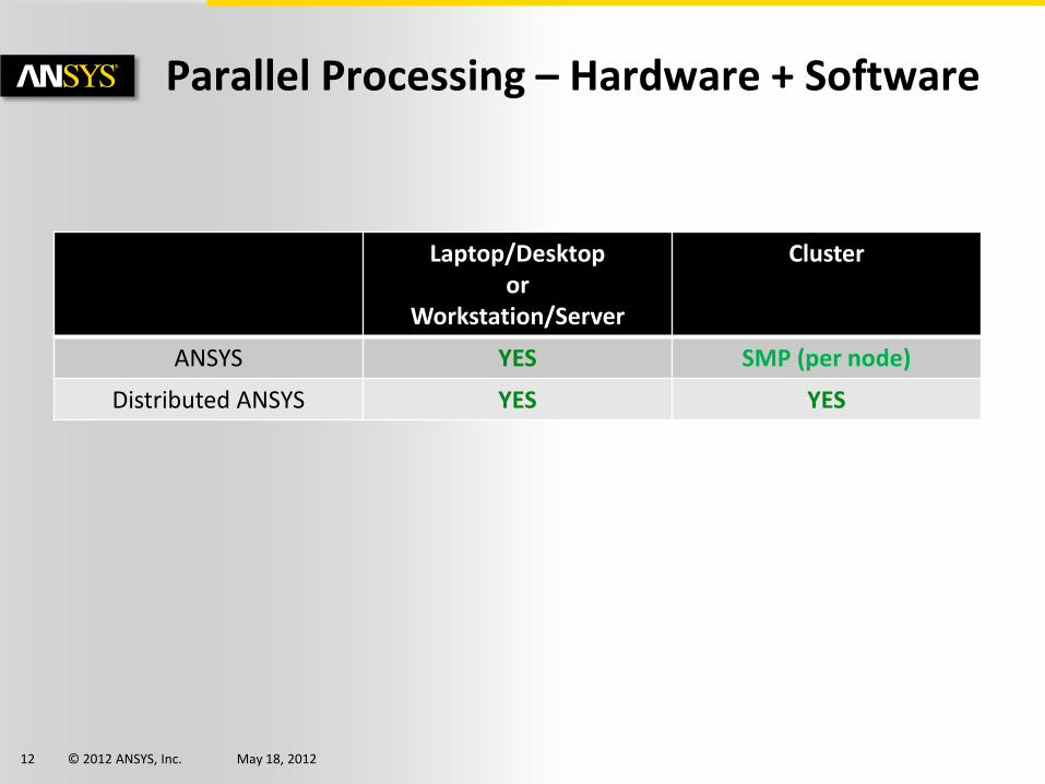
Parallel Processing – Hardware + Software
Laptop/Desktop or
Workstation/Server
Cluster
ANSYS YES SMP (per node)
Distributed ANSYS YES YES
© 2012 ANSYS, Inc. May 18, 2012 13
No limitation in simulation capability
Reproducible and consistent results
Support all major platforms
Distributed ANSYS Design Requirements
© 2012 ANSYS, Inc. May 18, 2012 14
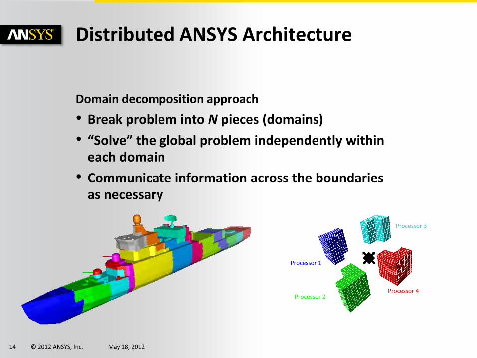
Domain decomposition approach
• Break problem into N pieces (domains)
• “Solve” the global problem independently within each domain
• Communicate information across the boundaries as necessary
Distributed ANSYS Architecture
Processor 1
Processor 4
Processor 3
Processor 2
© 2012 ANSYS, Inc. May 18, 2012 15
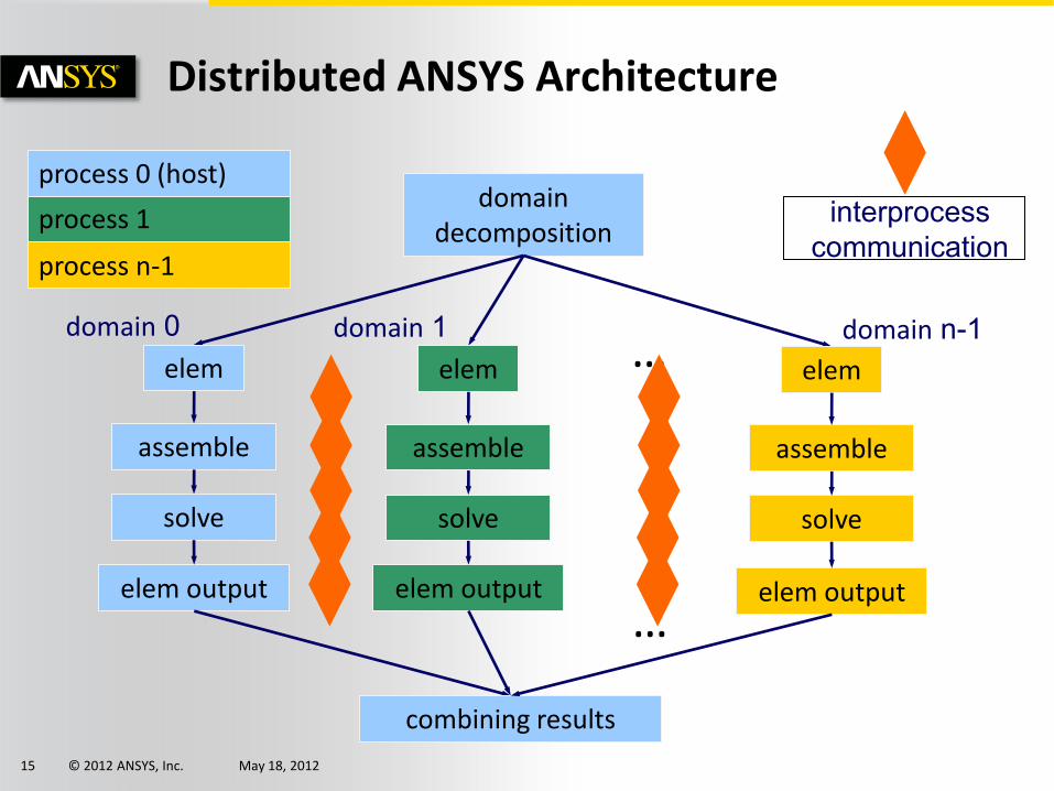
Distributed ANSYS Architecture
domain 0
interprocess communication
process 1
process 0 (host)
process n-1
domain decomposition
…
elem
assemble
solve
domain 1 domain n-1 elem
assemble
solve
elem
assemble
solve
elem output elem output elem output
…
combining results
© 2012 ANSYS, Inc. May 18, 2012 16
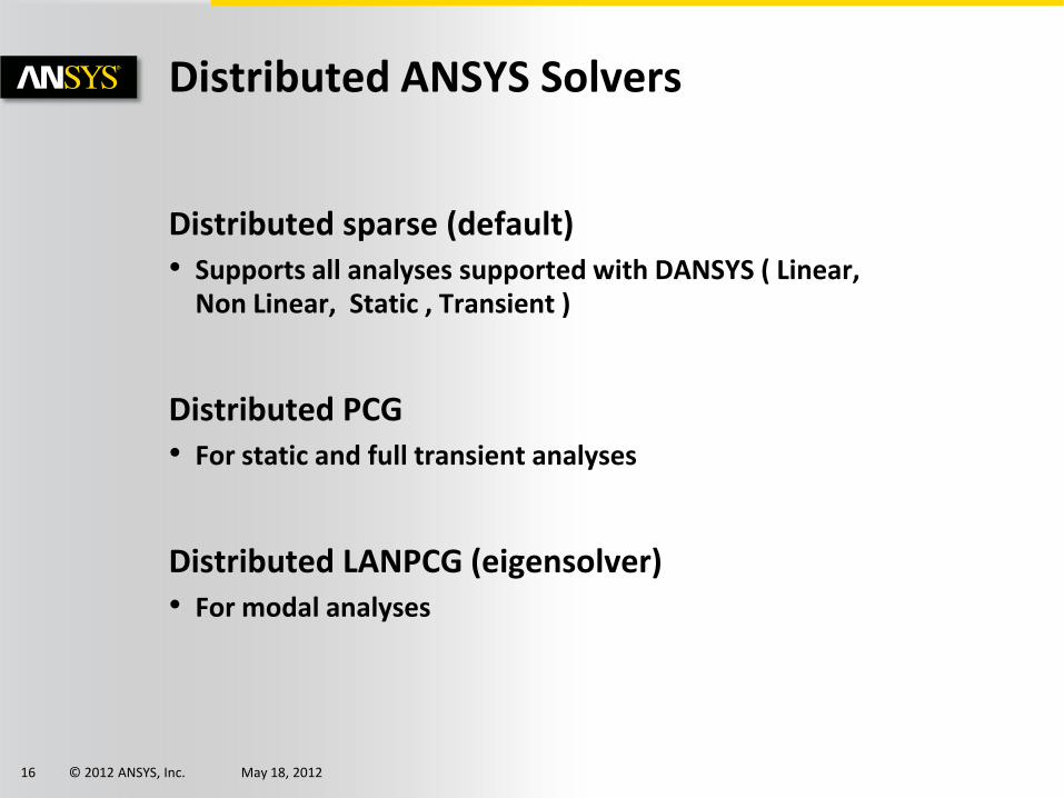
Distributed sparse (default) • Supports all analyses supported with DANSYS ( Linear,
Non Linear, Static , Transient )
Distributed PCG • For static and full transient analyses
Distributed LANPCG (eigensolver) • For modal analyses
Distributed ANSYS Solvers
© 2012 ANSYS, Inc. May 18, 2012 17
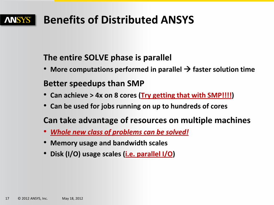
The entire SOLVE phase is parallel
• More computations performed in parallel faster solution time
Better speedups than SMP • Can achieve > 4x on 8 cores (Try getting that with SMP!!!!)
• Can be used for jobs running on up to hundreds of cores
Can take advantage of resources on multiple machines • Whole new class of problems can be solved!
• Memory usage and bandwidth scales
• Disk (I/O) usage scales (i.e. parallel I/O)
Benefits of Distributed ANSYS
© 2012 ANSYS, Inc. May 18, 2012 18
Basic information Solver Configuration Information during
the solve Output data
A model :
-Size / number of DOF -Analysis type
A machine : -Number of cores -RAM
Parallel Processing Method : -Shared Memory (SMP) -Distributed Memory (DMP)
Solver type : -Direct (Sparse) -Iterative (PCG)
Memory Settings
Resource Monitor :
-CPU -Memory -Disk -Network
-Elapsed Time
-Equation solver computational rate
-Equation solver effective I/O rate (Bandwidth)
-Total memory used (incore/out-of-core?)
Solver Types
© 2012 ANSYS, Inc. May 18, 2012 19
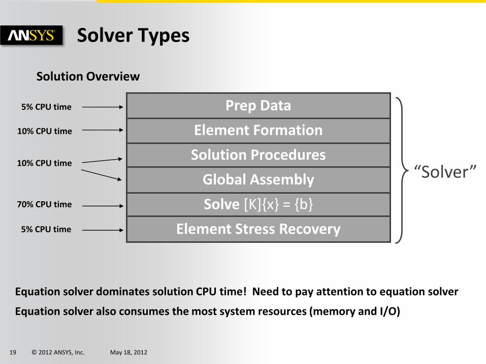
Solution Overview
Solver Types
Equation solver dominates solution CPU time! Need to pay attention to equation solver
Equation solver also consumes the most system resources (memory and I/O)
“Solver”
Solve [K]{x} = {b}
Solution Procedures
Element Formation
Prep Data
Element Stress Recovery
Global Assembly
10% CPU time
5% CPU time
10% CPU time
70% CPU time
5% CPU time
© 2012 ANSYS, Inc. May 18, 2012 20
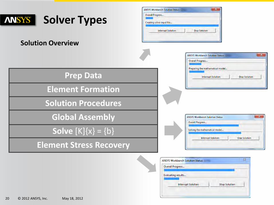
Solution Overview
Solver Types
Solve [K]{x} = {b}
Solution Procedures
Element Formation
Prep Data
Element Stress Recovery
Global Assembly
© 2012 ANSYS, Inc. May 18, 2012 21
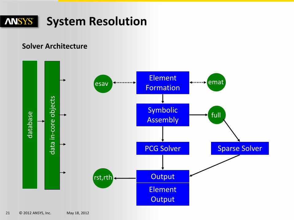
Solver Architecture
System Resolution
emat
full
Element Formation
Output
Symbolic Assembly
PCG Solver
dat
a in
-co
re o
bje
cts
dat
abas
e
Element Output
Sparse Solver
esav
rst,rth
© 2012 ANSYS, Inc. May 18, 2012 22
SPARSE (Direct)
Filing …
LN09
*.BCS: Stats from Sparse Solver
*.full: Assembled Stiffness Matrix
Solver Types: SPARSE (Direct)
© 2012 ANSYS, Inc. May 18, 2012 23
SPARSE (Direct)
PROS
- More robust with poorly conditioned problems (Shell-Beams)
- Solution always guaranteed
- Fast for 2nd Solve or Higher (Multiple Load cases)
CONS
- Factoring matrix & Solving are resource intensive
- Large memory requirements
Solver Types: SPARSE (Direct)
© 2012 ANSYS, Inc. May 18, 2012 24
PCG (Iterative)
- Minimization of residuals/potential energy (Standard Conjugate Gradient Method) ( {r} = {f} – [K].{u} )
- Iterative process requiring a convergence test (PCGTOL).
- Preconjugate CG used instead to reduce the number of iterations ( Preconditioner [Q] ̴ [K-1] - [Q] cheaper than [K-1] )
- Number of iterations
Solver Types: PCG (Iterative)
© 2012 ANSYS, Inc. May 18, 2012 25
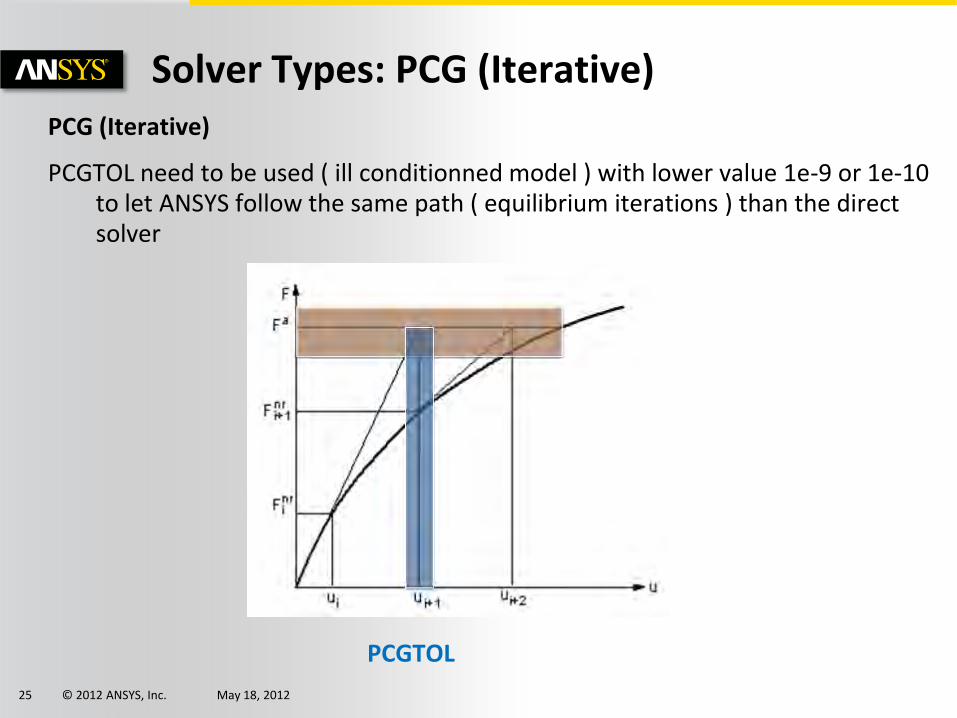
PCG (Iterative)
PCGTOL need to be used ( ill conditionned model ) with lower value 1e-9 or 1e-10 to let ANSYS follow the same path ( equilibrium iterations ) than the direct solver
Solver Types: PCG (Iterative)
PCGTOL
© 2012 ANSYS, Inc. May 18, 2012 26
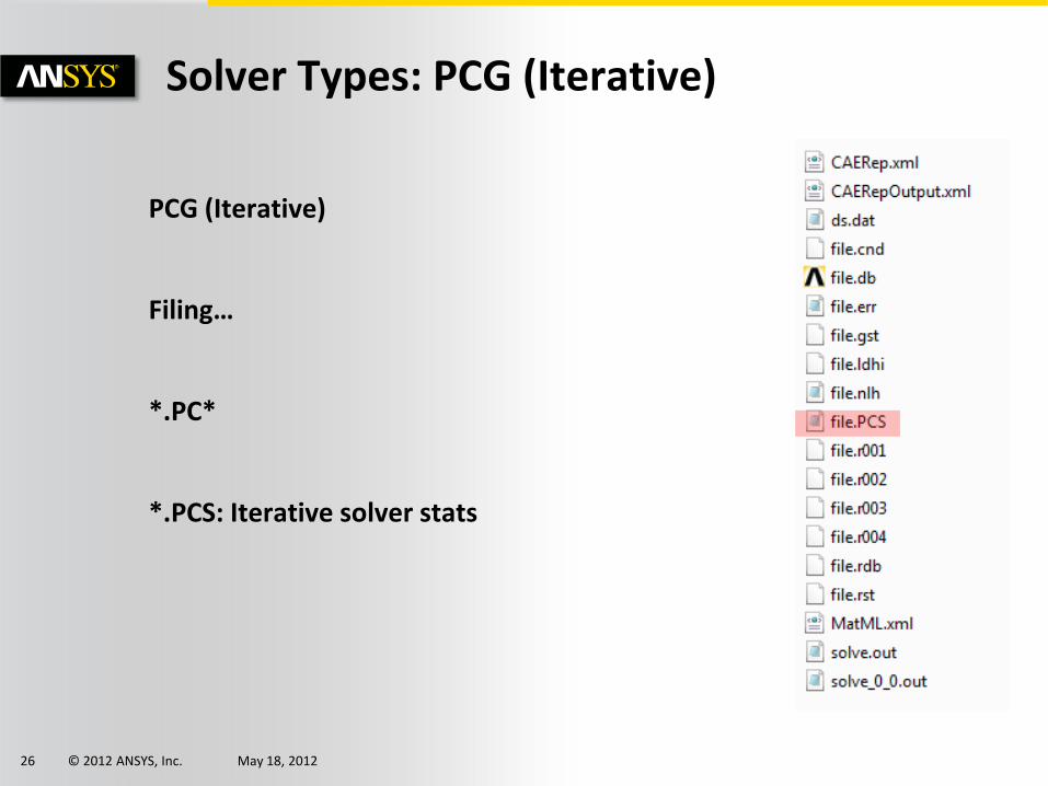
PCG (Iterative)
Filing…
*.PC*
*.PCS: Iterative solver stats
Solver Types: PCG (Iterative)
© 2012 ANSYS, Inc. May 18, 2012 27
PCG (Iterative)
PROS
- Less memory requirements
- Better suited for well conditioned bigger problem
CONS
- Not useful with near or rigid body behavior
- Less robust with ill-conditioned models (Shells & Beams, inadequate boundary conditions (Rigid Body Motions), elements considerably elongated, nearly singular matrices…) – more difficult to approximate [K-1] with [Q]
Solver Types: PCG (Iterative)
© 2012 ANSYS, Inc. May 18, 2012 28
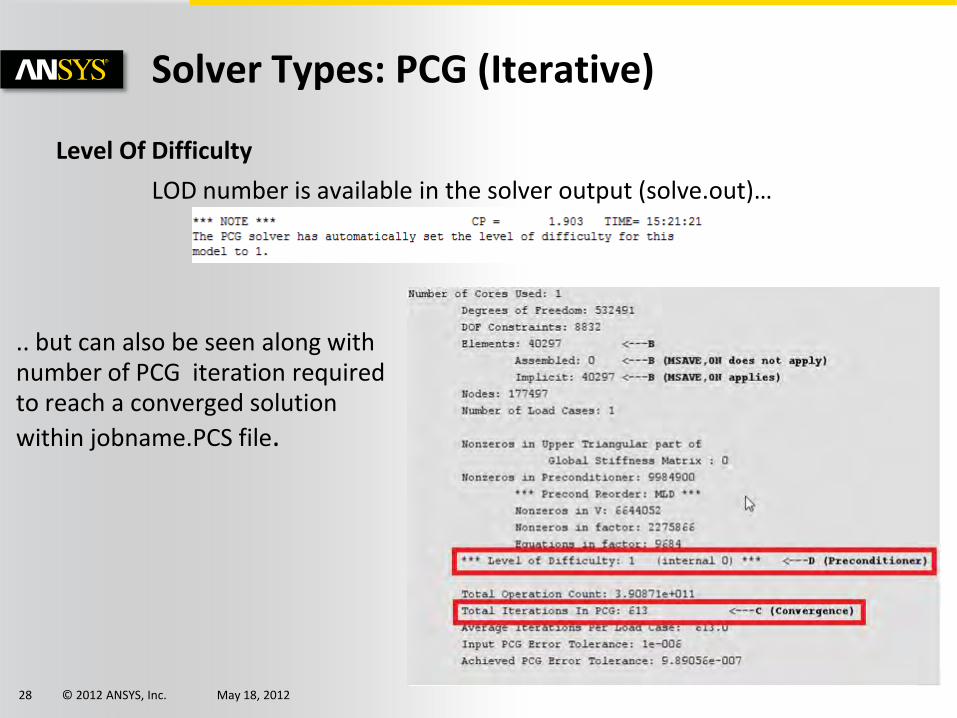
Level Of Difficulty
Solver Types: PCG (Iterative)
.. but can also be seen along with number of PCG iteration required to reach a converged solution
within jobname.PCS file.
LOD number is available in the solver output (solve.out)…
© 2012 ANSYS, Inc. May 18, 2012 29
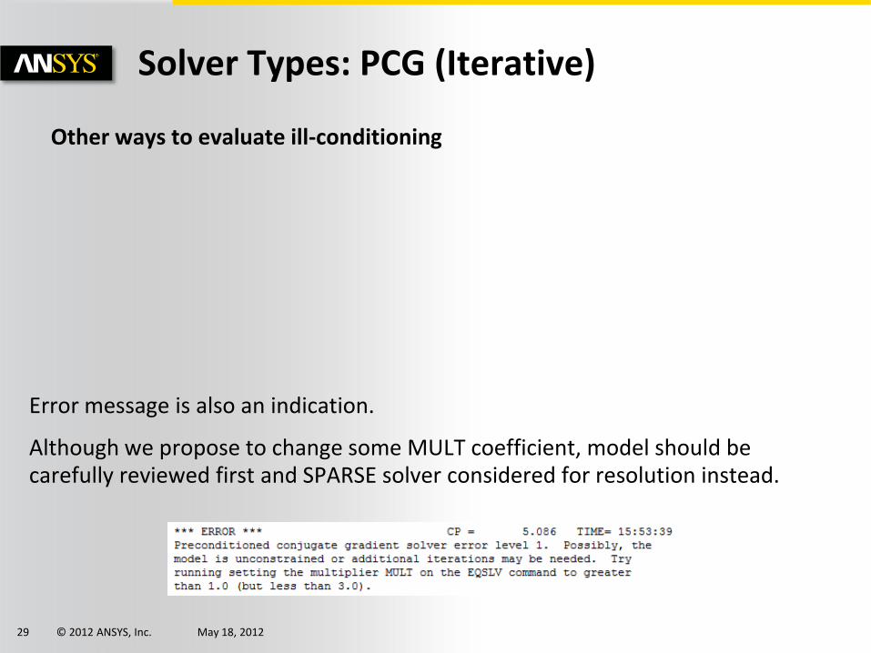
Other ways to evaluate ill-conditioning
Solver Types: PCG (Iterative)
Error message is also an indication.
Although we propose to change some MULT coefficient, model should be carefully reviewed first and SPARSE solver considered for resolution instead.
© 2012 ANSYS, Inc. May 18, 2012 30
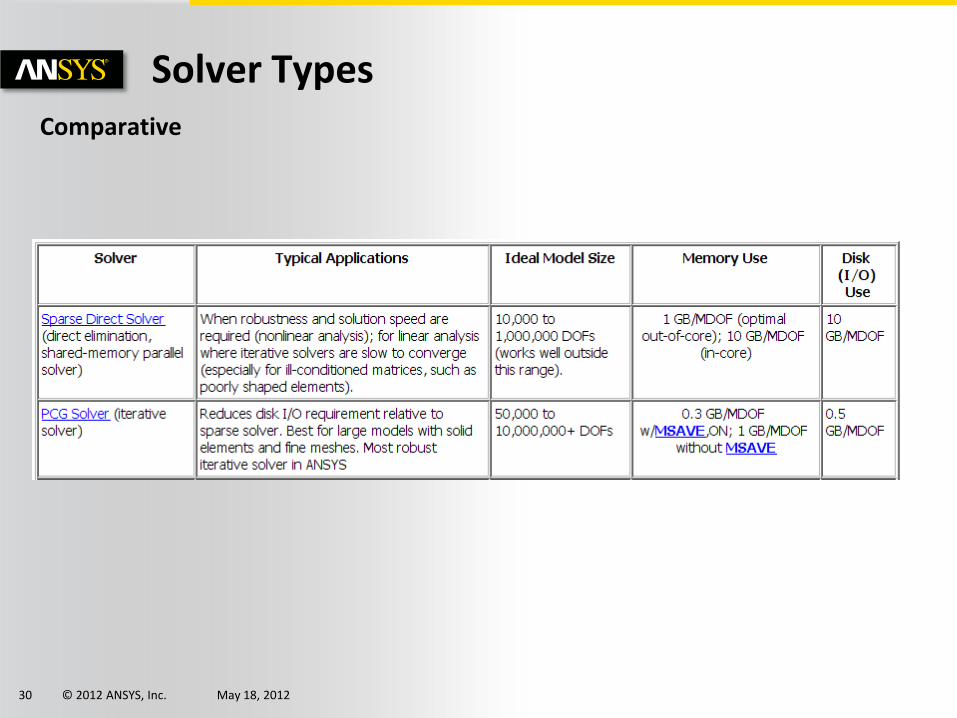
Comparative
Solver Types
© 2012 ANSYS, Inc. May 18, 2012 31
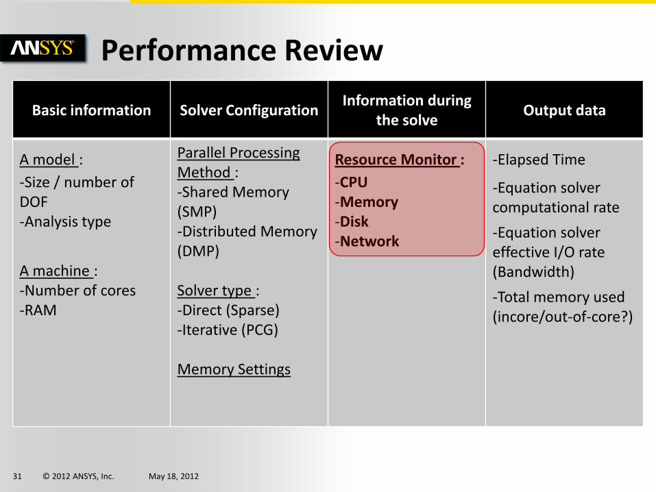
Basic information Solver Configuration Information during
the solve Output data
A model :
-Size / number of DOF -Analysis type
A machine : -Number of cores -RAM
Parallel Processing Method : -Shared Memory (SMP) -Distributed Memory (DMP)
Solver type : -Direct (Sparse) -Iterative (PCG)
Memory Settings
Resource Monitor :
-CPU -Memory -Disk -Network
-Elapsed Time
-Equation solver computational rate
-Equation solver effective I/O rate (Bandwidth)
-Total memory used (incore/out-of-core?)
Performance Review
© 2012 ANSYS, Inc. May 18, 2012 32
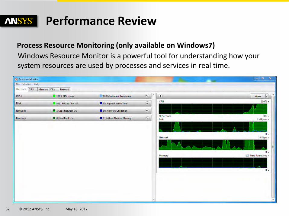
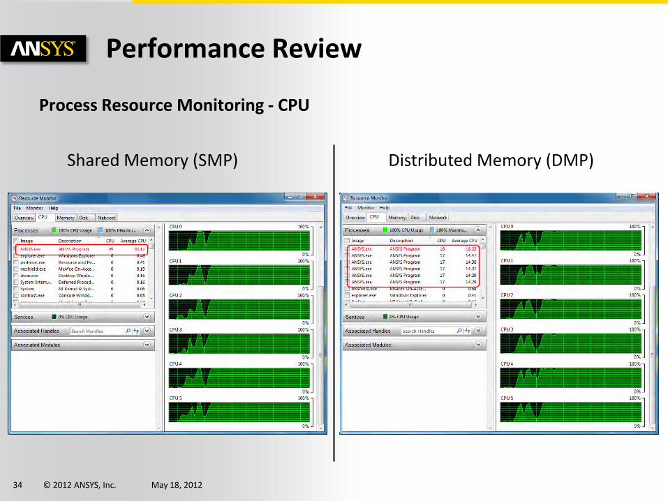
Process Resource Monitoring (only available on Windows7)
Performance Review
Windows Resource Monitor is a powerful tool for understanding how your system resources are used by processes and services in real time.
© 2012 ANSYS, Inc. May 18, 2012 33
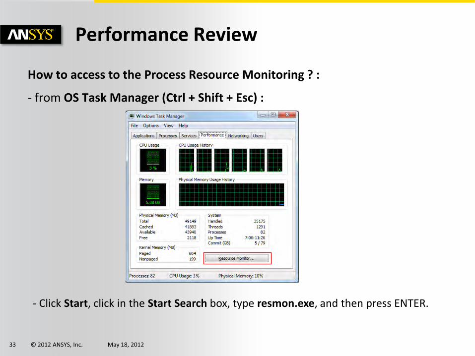
How to access to the Process Resource Monitoring ? :
- from OS Task Manager (Ctrl + Shift + Esc) :
Performance Review
- Click Start, click in the Start Search box, type resmon.exe, and then press ENTER.
© 2012 ANSYS, Inc. May 18, 2012 34
Process Resource Monitoring - CPU
Performance Review
Shared Memory (SMP) Distributed Memory (DMP)
© 2012 ANSYS, Inc. May 18, 2012 35
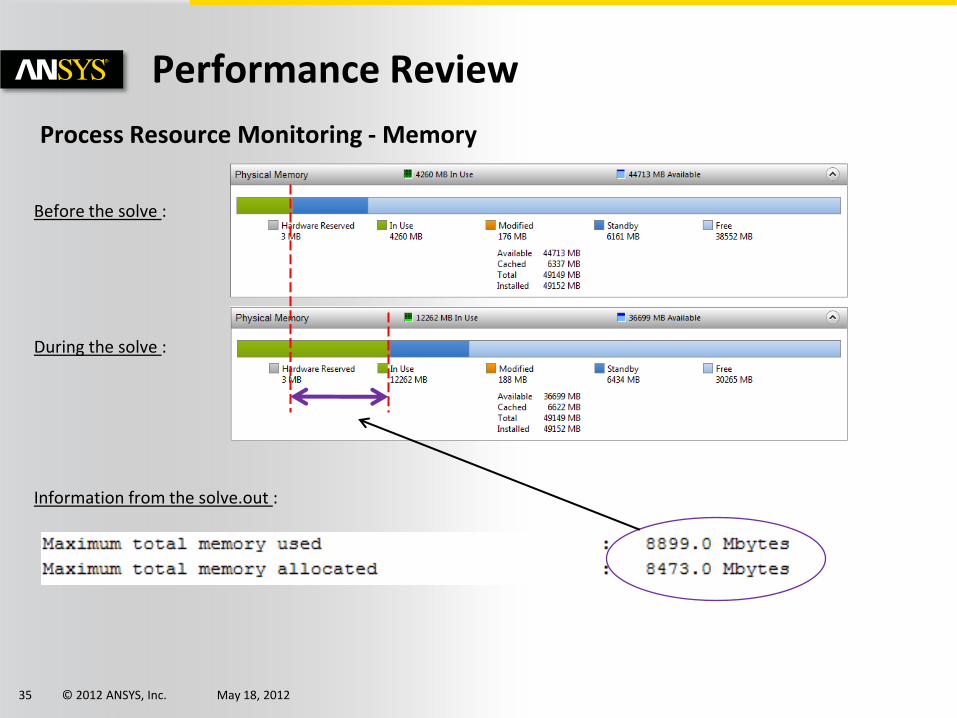
Process Resource Monitoring - Memory
Performance Review
Before the solve :
During the solve :
Information from the solve.out :
© 2012 ANSYS, Inc. May 18, 2012 36
Basic information Solver Configuration Information during
the solve Output data
A model :
-Size / number of DOF -Analysis type
A machine : -Number of cores -RAM
Parallel Processing Method : -Shared Memory (SMP) -Distributed Memory (DMP)
Solver type : -Direct (Sparse) -Iterative (PCG)
Memory Settings
Resource Monitor :
-CPU -Memory -Disk -Network
-Elapsed Time
-Equation solver computational rate
-Equation solver effective I/O rate (Bandwidth)
-Total memory used (incore/out-of-core?)
Overview
© 2012 ANSYS, Inc. May 18, 2012 37
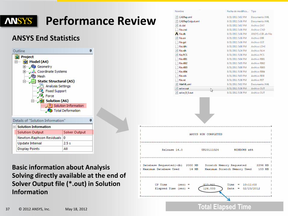
ANSYS End Statistics
Performance Review
Basic information about Analysis Solving directly available at the end of Solver Output file (*.out) in Solution Information
Total Elapsed Time
© 2012 ANSYS, Inc. May 18, 2012 38
Performance Review
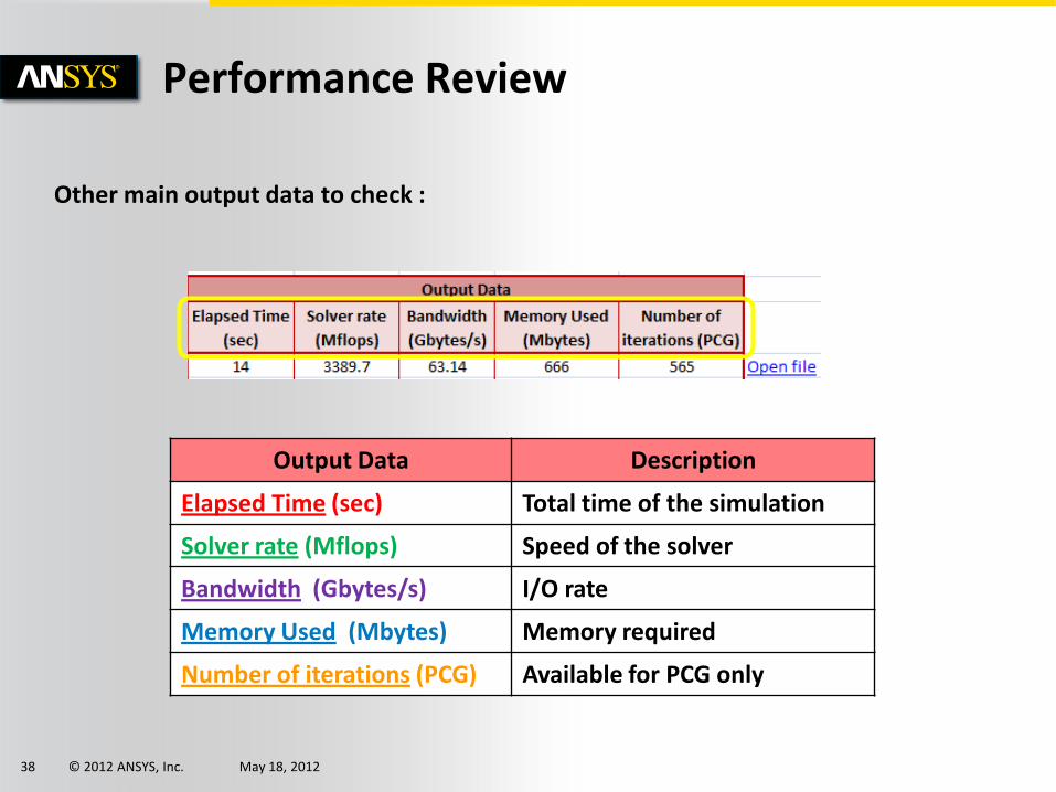
Output Data Description
Elapsed Time (sec) Total time of the simulation
Solver rate (Mflops) Speed of the solver
Bandwidth (Gbytes/s) I/O rate
Memory Used (Mbytes) Memory required
Number of iterations (PCG) Available for PCG only
Other main output data to check :
© 2012 ANSYS, Inc. May 18, 2012 39
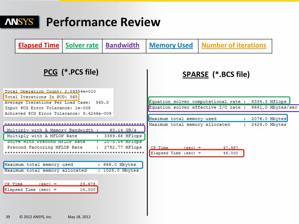
Performance Review
Elapsed Time Solver rate Bandwidth Memory Used Number of iterations
PCG (*.PCS file) SPARSE (*.BCS file)
© 2012 ANSYS, Inc. May 18, 2012 40
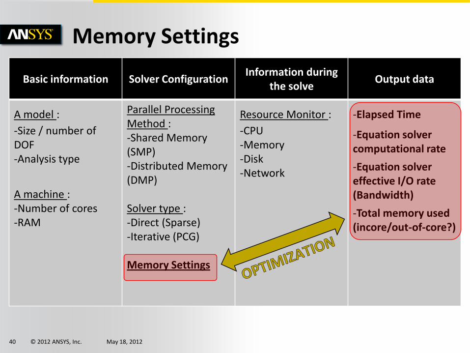
Basic information Solver Configuration Information during
the solve Output data
A model :
-Size / number of DOF -Analysis type
A machine : -Number of cores -RAM
Parallel Processing Method : -Shared Memory (SMP) -Distributed Memory (DMP)
Solver type : -Direct (Sparse) -Iterative (PCG)
Memory Settings
Resource Monitor :
-CPU -Memory -Disk -Network
-Elapsed Time
-Equation solver computational rate
-Equation solver effective I/O rate (Bandwidth)
-Total memory used (incore/out-of-core?)
Memory Settings
© 2012 ANSYS, Inc. May 18, 2012 41
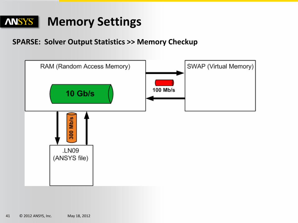
SPARSE: Solver Output Statistics >> Memory Checkup
Memory Settings
© 2012 ANSYS, Inc. May 18, 2012 42
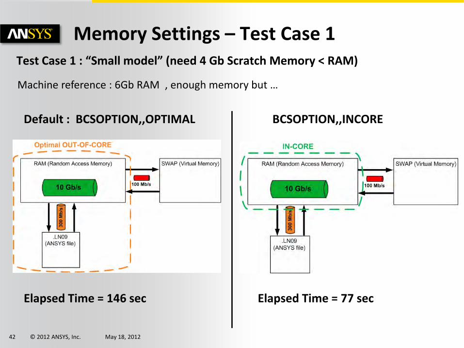
Memory Settings – Test Case 1 Test Case 1 : “Small model” (need 4 Gb Scratch Memory < RAM)
Default : BCSOPTION,,OPTIMAL BCSOPTION,,INCORE
Machine reference : 6Gb RAM , enough memory but …
Elapsed Time = 77 sec Elapsed Time = 146 sec
© 2012 ANSYS, Inc. May 18, 2012 43
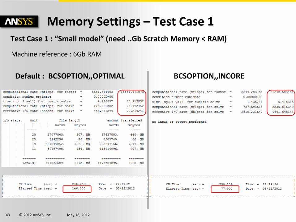
Memory Settings – Test Case 1 Test Case 1 : “Small model” (need ..Gb Scratch Memory < RAM)
Default : BCSOPTION,,OPTIMAL BCSOPTION,,INCORE
Machine reference : 6Gb RAM
© 2012 ANSYS, Inc. May 18, 2012 44
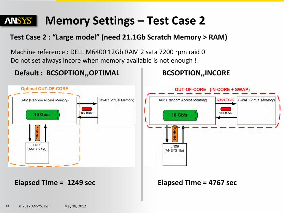
Memory Settings – Test Case 2
Default : BCSOPTION,,OPTIMAL BCSOPTION,,INCORE
Elapsed Time = 4767 sec Elapsed Time = 1249 sec
Test Case 2 : “Large model” (need 21.1Gb Scratch Memory > RAM)
Machine reference : DELL M6400 12Gb RAM 2 sata 7200 rpm raid 0 Do not set always incore when memory available is not enough !!
© 2012 ANSYS, Inc. May 18, 2012 45
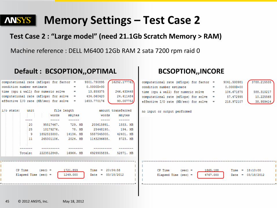
Memory Settings – Test Case 2
Default : BCSOPTION,,OPTIMAL BCSOPTION,,INCORE
Test Case 2 : “Large model” (need 21.1Gb Scratch Memory > RAM)
Machine reference : DELL M6400 12Gb RAM 2 sata 7200 rpm raid 0
© 2012 ANSYS, Inc. May 18, 2012 46
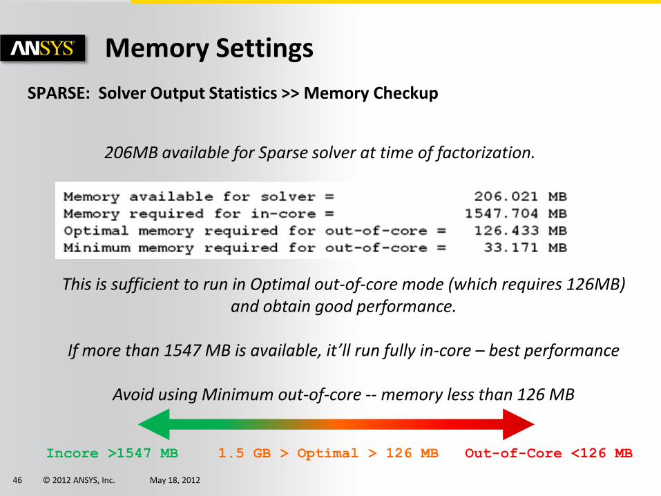
SPARSE: Solver Output Statistics >> Memory Checkup
Memory Settings
206MB available for Sparse solver at time of factorization.
This is sufficient to run in Optimal out-of-core mode (which requires 126MB) and obtain good performance.
If more than 1547 MB is available, it’ll run fully in-core – best performance
Avoid using Minimum out-of-core -- memory less than 126 MB
1.5 GB > Optimal > 126 MB Out-of-Core <126 MB Incore >1547 MB
© 2012 ANSYS, Inc. May 18, 2012 47
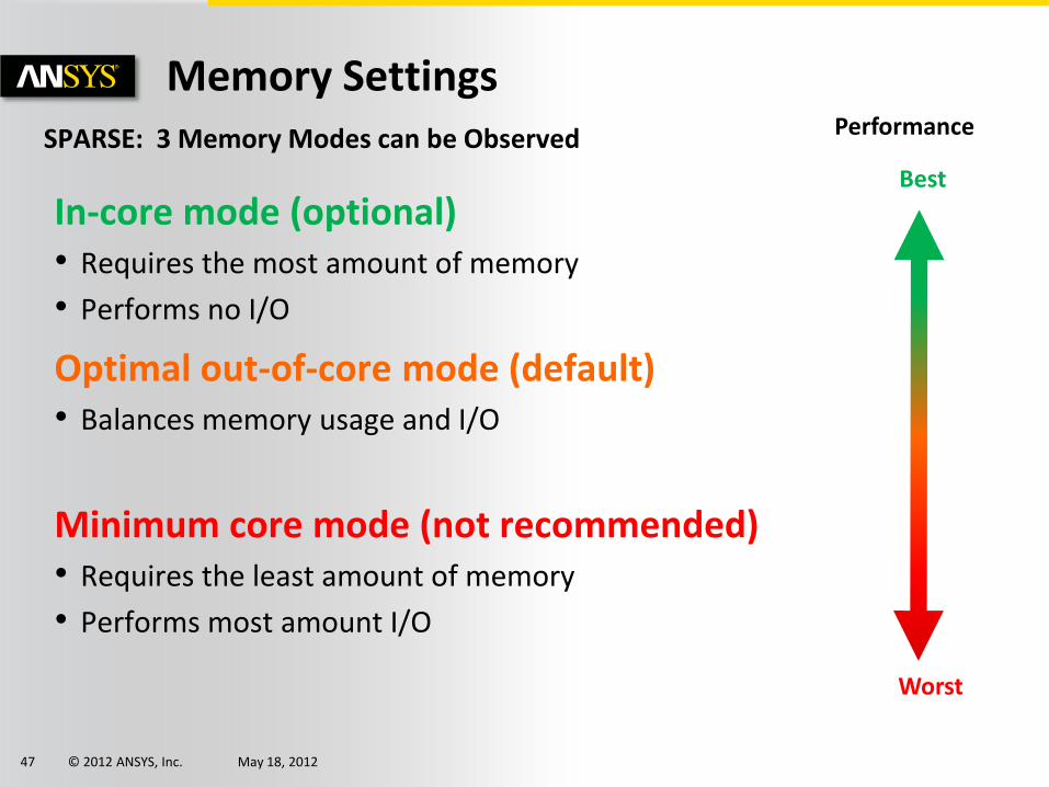
SPARSE: 3 Memory Modes can be Observed
Memory Settings
In-core mode (optional) • Requires the most amount of memory
• Performs no I/O
Optimal out-of-core mode (default) • Balances memory usage and I/O
Minimum core mode (not recommended) • Requires the least amount of memory
• Performs most amount I/O
Performance
Best
Worst
© 2012 ANSYS, Inc. May 18, 2012 48
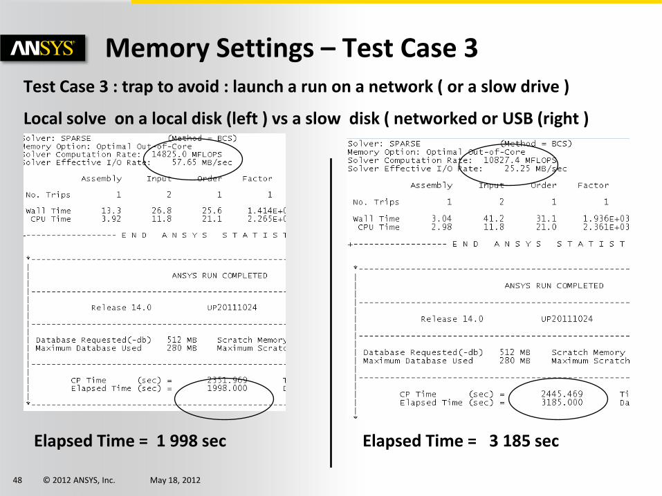
Memory Settings – Test Case 3
Elapsed Time = 1 998 sec Elapsed Time = 3 185 sec
Test Case 3 : trap to avoid : launch a run on a network ( or a slow drive )
Local solve on a local disk (left ) vs a slow disk ( networked or USB (right )
© 2012 ANSYS, Inc. May 18, 2012 49
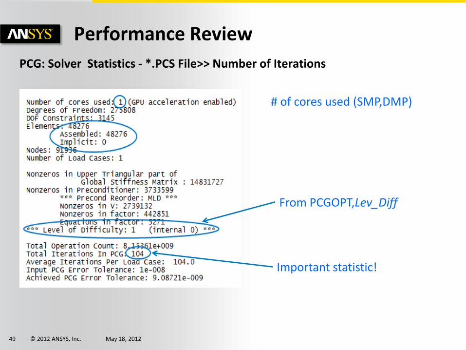
PCG: Solver Statistics - *.PCS File>> Number of Iterations
Performance Review
# of cores used (SMP,DMP)
From PCGOPT,Lev_Diff
Important statistic!
© 2012 ANSYS, Inc. May 18, 2012 50
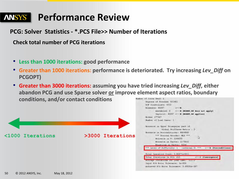
PCG: Solver Statistics - *.PCS File>> Number of Iterations
Performance Review
Check total number of PCG iterations
• Less than 1000 iterations: good performance
• Greater than 1000 iterations: performance is deteriorated. Try increasing Lev_Diff on PCGOPT)
• Greater than 3000 iterations: assuming you have tried increasing Lev_Diff, either abandon PCG and use Sparse solver or improve element aspect ratios, boundary conditions, and/or contact conditions
>3000 Iterations <1000 Iterations
© 2012 ANSYS, Inc. May 18, 2012 51
PCG: Solver Statistics - *.PCS File>> Number of Iterations
Performance Review
If too much iteration :
*Use parallel processing
• Use PCGOPT,lev
• Refine your mesh
• Check for too high stiffness
© 2012 ANSYS, Inc. May 18, 2012 52
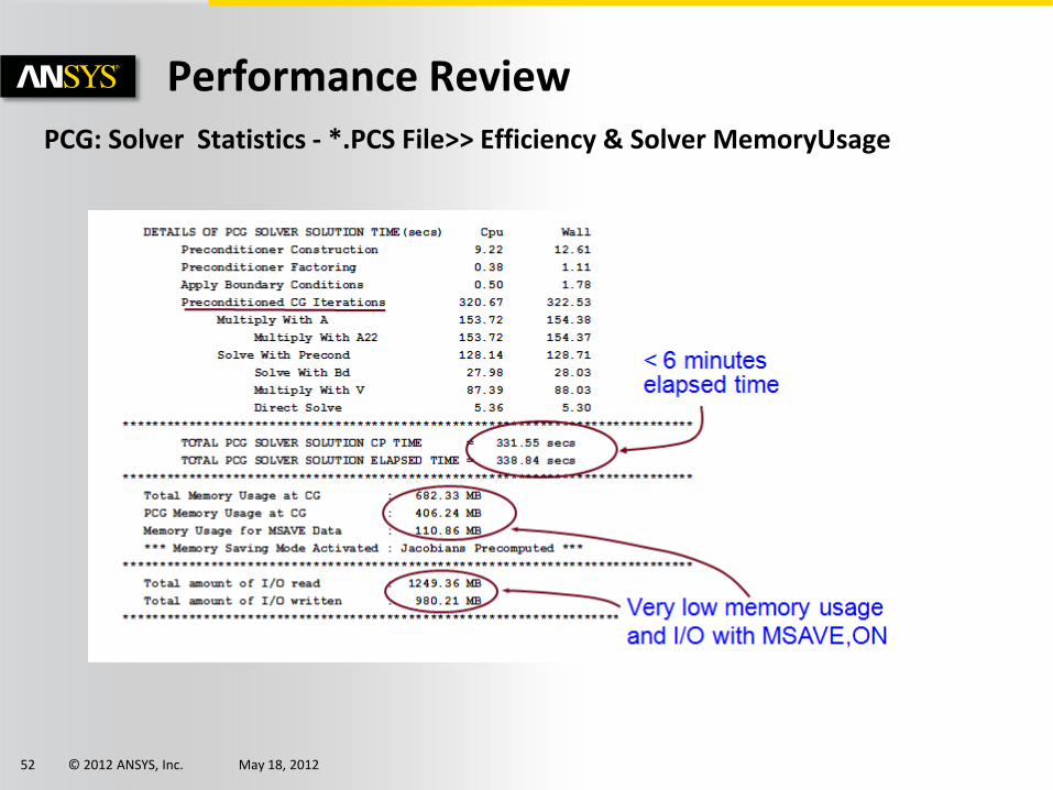
PCG: Solver Statistics - *.PCS File>> Efficiency & Solver MemoryUsage
Performance Review
© 2012 ANSYS, Inc. May 18, 2012 53
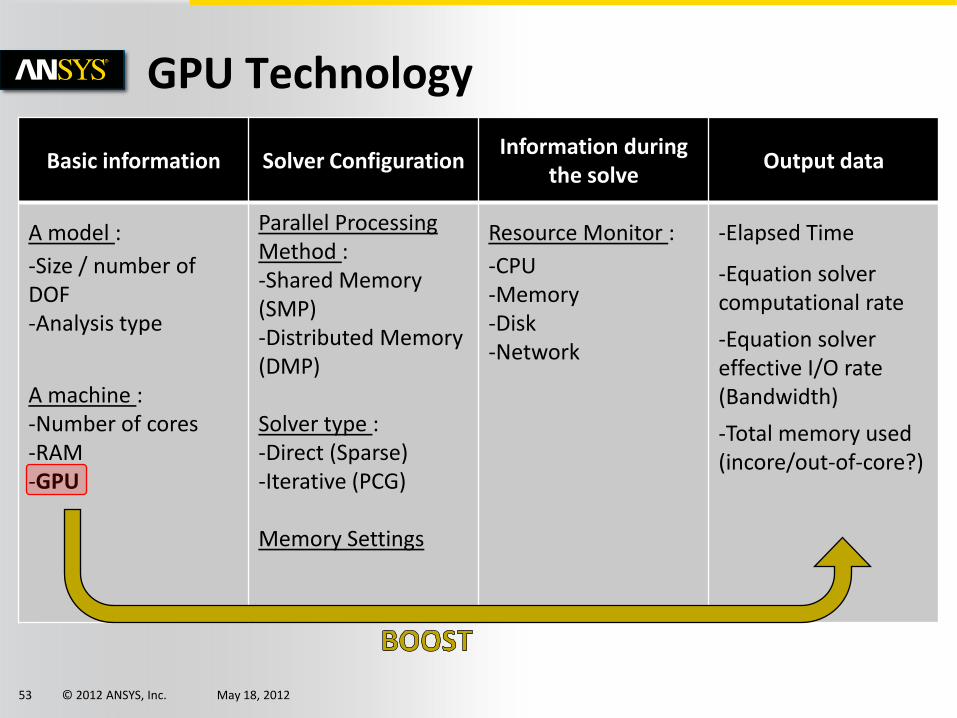
Basic information Solver Configuration Information during
the solve Output data
A model :
-Size / number of DOF -Analysis type
A machine : -Number of cores -RAM -GPU
Parallel Processing Method : -Shared Memory (SMP) -Distributed Memory (DMP)
Solver type : -Direct (Sparse) -Iterative (PCG)
Memory Settings
Resource Monitor :
-CPU -Memory -Disk -Network
-Elapsed Time
-Equation solver computational rate
-Equation solver effective I/O rate (Bandwidth)
-Total memory used (incore/out-of-core?)
GPU Technology
© 2012 ANSYS, Inc. May 18, 2012 54
Graphics processing units (GPUs) • Widely used for gaming, graphics rendering
• Recently been made available as general-purpose “accelerators”
– Support for double precision arithmetic
– Performance exceeding the latest multicore CPUs
• So how can ANSYS Mechanical make use of this new technology to reduce the overall time to solution??
GPU Technology
© 2012 ANSYS, Inc. May 18, 2012 55
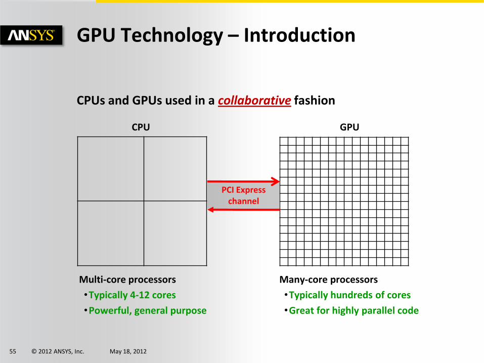
CPUs and GPUs used in a collaborative fashion
GPU Technology – Introduction
Multi-core processors
•Typically 4-12 cores
•Powerful, general purpose
Many-core processors
•Typically hundreds of cores
•Great for highly parallel code
CPU GPU
PCI Express channel
© 2012 ANSYS, Inc. May 18, 2012 56
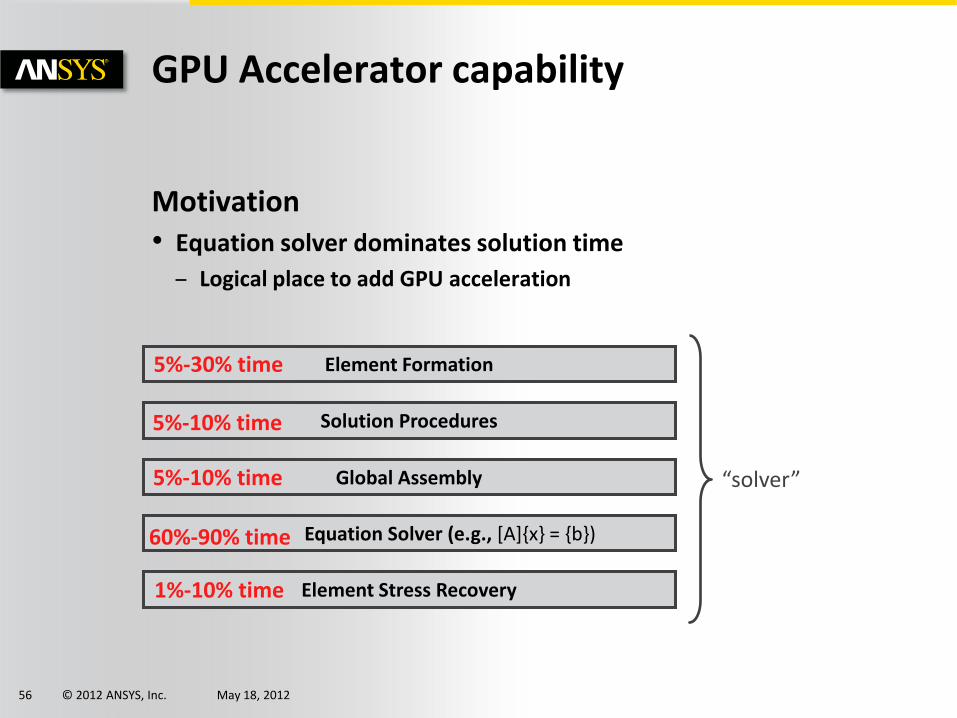
Motivation • Equation solver dominates solution time
– Logical place to add GPU acceleration
GPU Accelerator capability
“solver”
Equation Solver (e.g., [A]{x} = {b})
Solution Procedures
Element Formation
Element Stress Recovery
Global Assembly
5%-30% time
1%-10% time
5%-10% time
60%-90% time
5%-10% time
© 2012 ANSYS, Inc. May 18, 2012 57
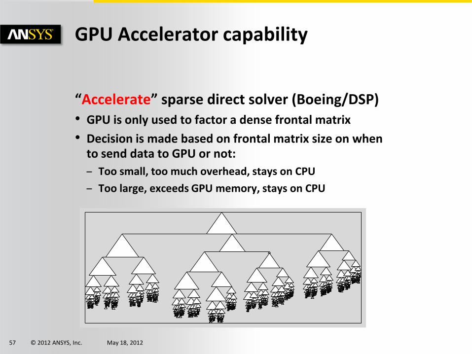
“Accelerate” sparse direct solver (Boeing/DSP) • GPU is only used to factor a dense frontal matrix
• Decision is made based on frontal matrix size on when to send data to GPU or not:
– Too small, too much overhead, stays on CPU
– Too large, exceeds GPU memory, stays on CPU
GPU Accelerator capability
© 2012 ANSYS, Inc. May 18, 2012 58
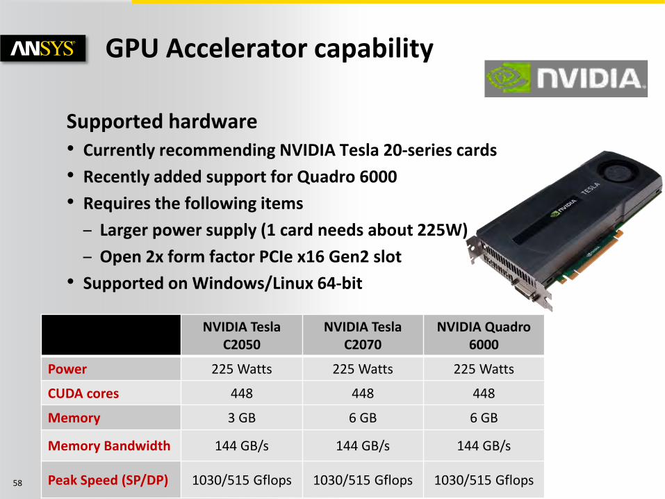
Supported hardware • Currently recommending NVIDIA Tesla 20-series cards
• Recently added support for Quadro 6000
• Requires the following items
– Larger power supply (1 card needs about 225W)
– Open 2x form factor PCIe x16 Gen2 slot
• Supported on Windows/Linux 64-bit
GPU Accelerator capability
NVIDIA Tesla C2050
NVIDIA Tesla C2070
NVIDIA Quadro 6000
Power 225 Watts 225 Watts 225 Watts
CUDA cores 448 448 448
Memory 3 GB 6 GB 6 GB
Memory Bandwidth 144 GB/s 144 GB/s 144 GB/s
Peak Speed (SP/DP) 1030/515 Gflops 1030/515 Gflops 1030/515 Gflops
© 2012 ANSYS, Inc. May 18, 2012 59
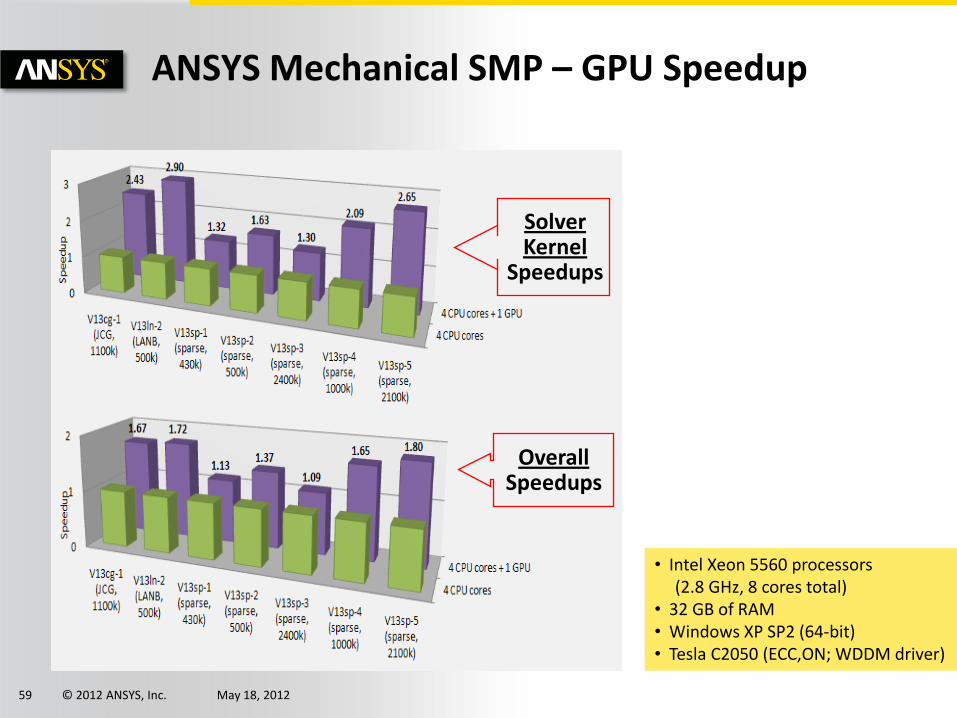
Solver Kernel
Speedups
Overall Speedups
ANSYS Mechanical SMP – GPU Speedup
• Intel Xeon 5560 processors (2.8 GHz, 8 cores total) • 32 GB of RAM • Windows XP SP2 (64-bit) • Tesla C2050 (ECC,ON; WDDM driver)
© 2012 ANSYS, Inc. May 18, 2012 60
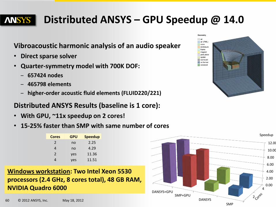
Distributed ANSYS – GPU Speedup @ 14.0
Cores GPU Speedup
2 no 2.25
4 no 4.29
2 yes 11.36
4 yes 11.51
Vibroacoustic harmonic analysis of an audio speaker
• Direct sparse solver
• Quarter-symmetry model with 700K DOF:
– 657424 nodes
– 465798 elements
– higher-order acoustic fluid elements (FLUID220/221)
Distributed ANSYS Results (baseline is 1 core):
• With GPU, ~11x speedup on 2 cores!
• 15-25% faster than SMP with same number of cores
Windows workstation: Two Intel Xeon 5530 processors (2.4 GHz, 8 cores total), 48 GB RAM, NVIDIA Quadro 6000
Speedup
SMP DANSYS
SMP+GPU DANSYS+GPU
0.00
2.00
4.00
6.00
8.00
10.00
12.00
2
4
© 2012 ANSYS, Inc. May 18, 2012 61
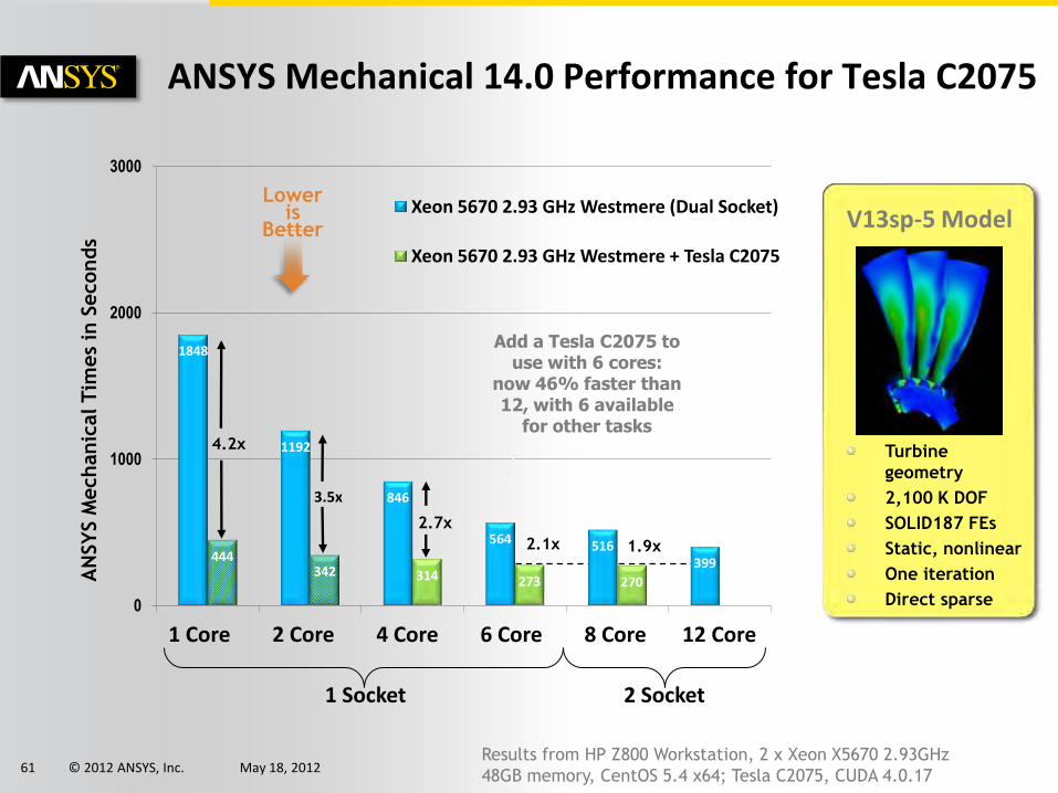
1848
1192
846
564 516 399 444
342 314 273 270
0
1000
2000
3000
Xeon 5670 2.93 GHz Westmere (Dual Socket)
Xeon 5670 2.93 GHz Westmere + Tesla C2075
AN
SY
S M
echanic
al Tim
es
in S
econds
4.2x
2.7x
3.5x
2.1x 1.9x
Add a Tesla C2075 to use with 6 cores:
now 46% faster than 12, with 6 available
for other tasks
1 Core 2 Core 4 Core 6 Core 12 Core
1 Socket 2 Socket
8 Core
Results from HP Z800 Workstation, 2 x Xeon X5670 2.93GHz
48GB memory, CentOS 5.4 x64; Tesla C2075, CUDA 4.0.17
V13sp-5 Model
Turbine
geometry
2,100 K DOF
SOLID187 FEs
Static, nonlinear
One iteration
Direct sparse
Lower is
Better
ANSYS Mechanical 14.0 Performance for Tesla C2075
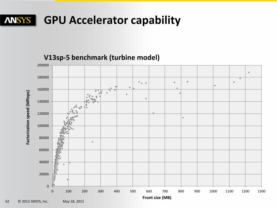
© 2012 ANSYS, Inc. May 18, 2012 62
V13sp-5 benchmark (turbine model)
GPU Accelerator capability
0
20000
40000
60000
80000
100000
120000
140000
160000
180000
200000
0 100 200 300 400 500 600 700 800 900 1000 1100 1200 1300
Fact
ori
zati
on
sp
eed
(M
flo
ps)
Front size (MB)
© 2012 ANSYS, Inc. May 18, 2012 63
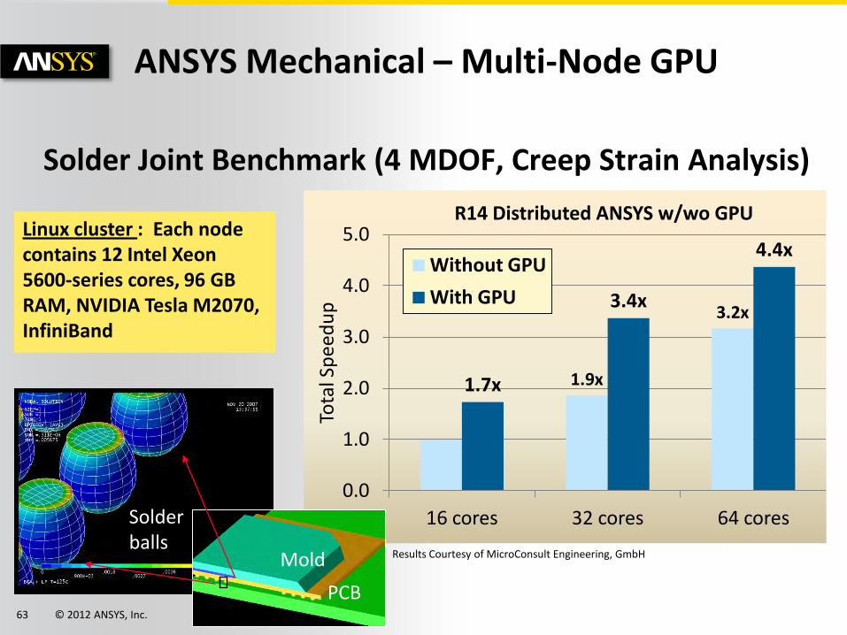
1.9x
3.2x
1.7x
3.4x
4.4x
0.0
1.0
2.0
3.0
4.0
5.0
16 cores 32 cores 64 cores
Tota
l Sp
eed
up
R14 Distributed ANSYS w/wo GPU
Without GPU
With GPU
ANSYS Mechanical – Multi-Node GPU
Mold
PCB
Solder balls
Results Courtesy of MicroConsult Engineering, GmbH
Solder Joint Benchmark (4 MDOF, Creep Strain Analysis)
Linux cluster : Each node contains 12 Intel Xeon 5600-series cores, 96 GB RAM, NVIDIA Tesla M2070, InfiniBand
© 2012 ANSYS, Inc. May 18, 2012 64
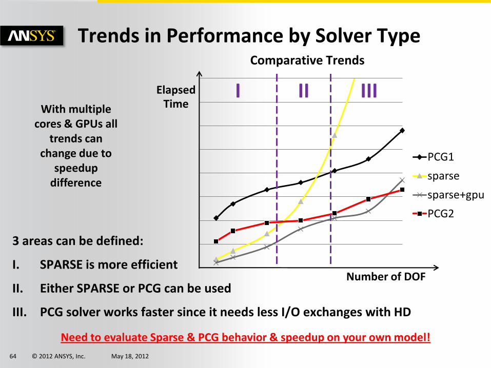
Comparative Trends
Trends in Performance by Solver Type
3 areas can be defined:
I. SPARSE is more efficient
II. Either SPARSE or PCG can be used
III. PCG solver works faster since it needs less I/O exchanges with HD
With multiple cores & GPUs all
trends can change due to
speedup difference
Need to evaluate Sparse & PCG behavior & speedup on your own model!
PCG1
sparse
sparse+gpu
PCG2
Number of DOF
Elapsed Time
I II III
© 2012 ANSYS, Inc. May 18, 2012 65
Tips and Tricks on performance gains • Some considerations on scalability of DANSYS
• Working with solution differences
• Working with a case that does not (or hardly) scale
• Working with programmable features for parallel runs
Other Software Considerations
© 2012 ANSYS, Inc. May 18, 2012 66
Scalability Considerations
Load balance
Improvements on domain decomposition
Amdahl’s Law • Algorithmic enhancements: every part of the code is to run in parallel
User controllable items:
• Contact pair definitions: big contact pairs hurt load balance (one contact pair is put into one domain in our code )
• CE definition: many CE terms hurt load balance and Amdahl’s law ( CE needs communications among domains that the CE’s are defined )
• Use best and most suitable hardware possible (speedup of the CPU, memory, I/O and interconnects)
© 2012 ANSYS, Inc. May 18, 2012 67
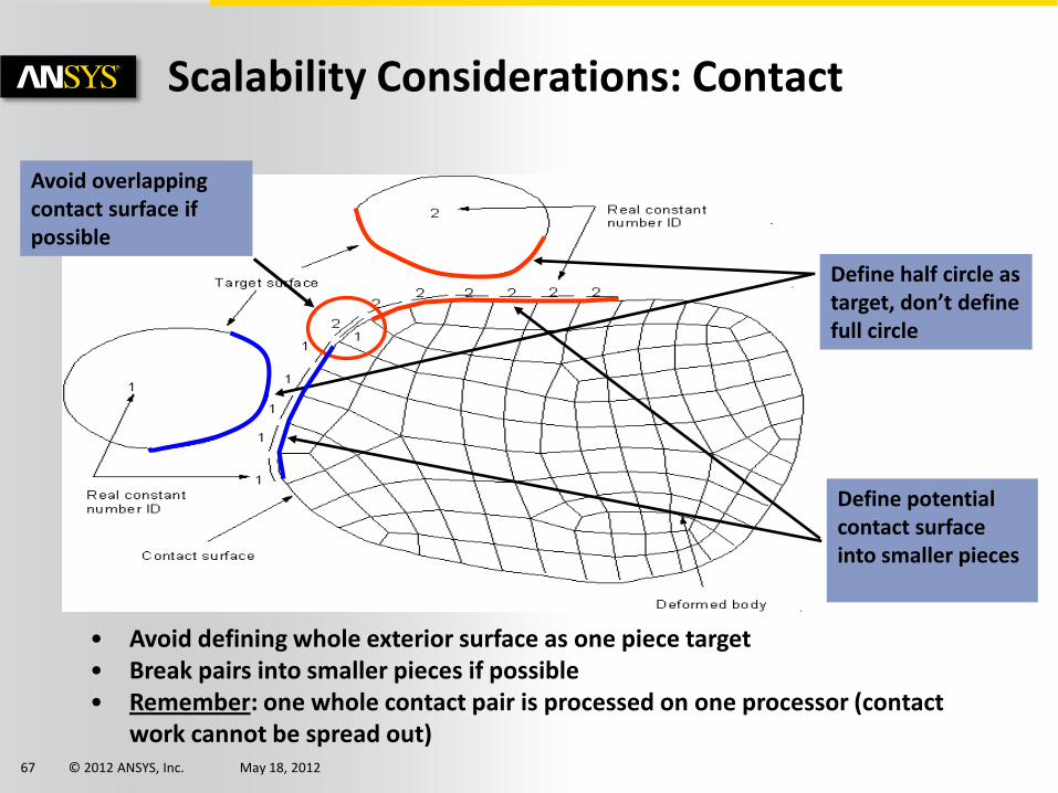
• Avoid defining whole exterior surface as one piece target • Break pairs into smaller pieces if possible • Remember: one whole contact pair is processed on one processor (contact
work cannot be spread out)
Define half circle as target, don’t define full circle
Avoid overlapping contact surface if possible
Define potential contact surface into smaller pieces
Scalability Considerations: Contact
© 2012 ANSYS, Inc. May 18, 2012 68
Scalability Considerations: Contact
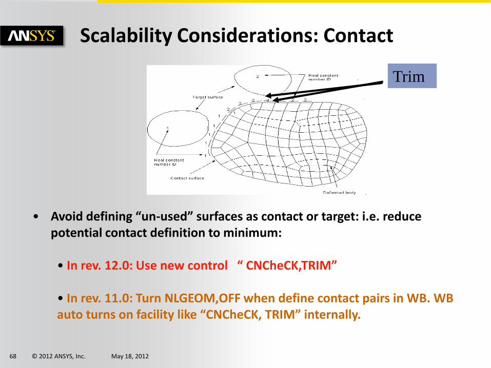
• Avoid defining “un-used” surfaces as contact or target: i.e. reduce potential contact definition to minimum:
• In rev. 12.0: Use new control “ CNCheCK,TRIM”
• In rev. 11.0: Turn NLGEOM,OFF when define contact pairs in WB. WB auto turns on facility like “CNCheCK, TRIM” internally.
Trim
© 2012 ANSYS, Inc. May 18, 2012 69
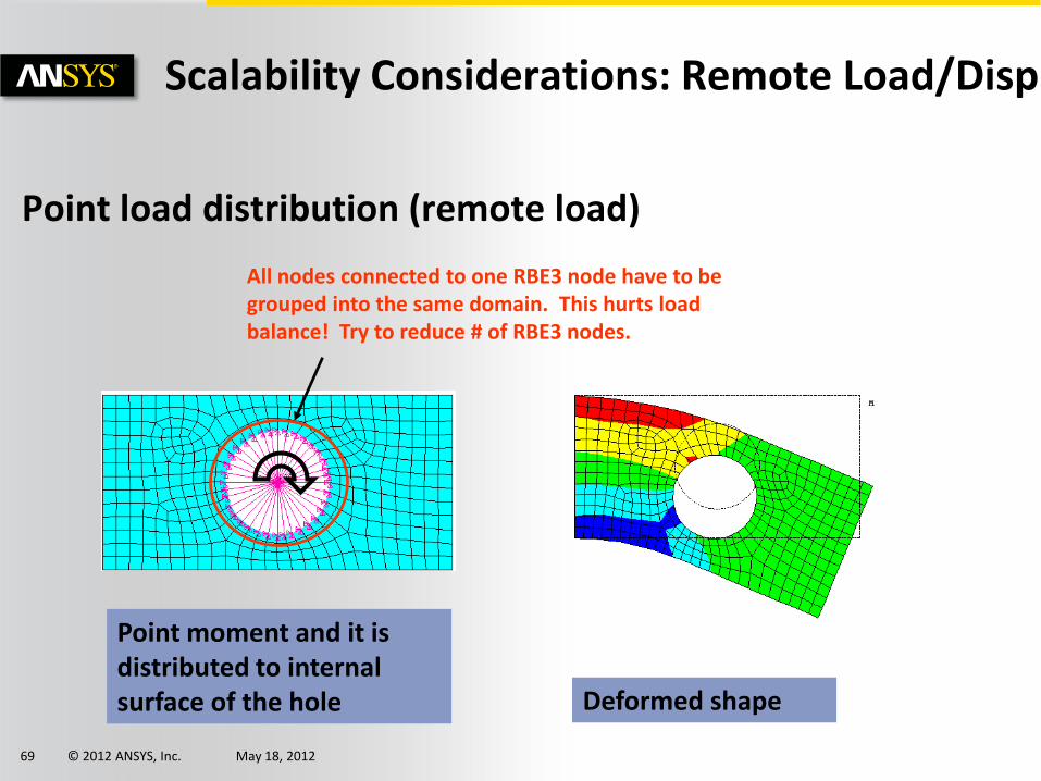
Point load distribution (remote load)
Point moment and it is distributed to internal surface of the hole Deformed shape
All nodes connected to one RBE3 node have to be grouped into the same domain. This hurts load balance! Try to reduce # of RBE3 nodes.
Scalability Considerations: Remote Load/Disp
© 2012 ANSYS, Inc. May 18, 2012 70
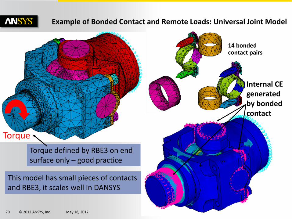
14 bonded contact pairs
Torque
Internal CE generated by bonded contact
Example of Bonded Contact and Remote Loads: Universal Joint Model
Torque defined by RBE3 on end surface only – good practice
This model has small pieces of contacts and RBE3, it scales well in DANSYS
© 2012 ANSYS, Inc. May 18, 2012 71
Working With Solution Differences in Parallel Runs
Most of solution differences come from contact applications when NP =1, versus NP = 2, 3, 4, 5, 6, 7, ……
• Check on contact pairs to make sure we don’t have a case of bifurcation and also plot deformations to see the case.
• Tighten CNVTOL convergence tolerance to see solution accuracy. If solution is less than, say, 1 % in difference, then parallel computing can make some difference in convergence, all solutions are acceptable.
• If solution is well-defined and all input settings are correct, report this case to ANSYS Inc. for investigations
© 2012 ANSYS, Inc. May 18, 2012 72
Working With a Case of Poor Scalability
No scalability (speedup) at all (or even slower than NP = 1)
• Is this problem too small (normally DOFs should be greater 50K)?
• Do I have a slow disk, problem is so big that I/O size exceeds the memory I/O buffer?
• Is every NODE of my machines connected to public network?
• Look at scalability at Solver first not the entire run (e.g. /prep7 time is mostly not scalable)
• Resume data at /solu level and don’t read in input files every time of the run
• etc
© 2012 ANSYS, Inc. May 18, 2012 73
Working With a Case of Poor Scalability
Yes, I have scalability but poor (say, speedup < 2X)
• Is this GigE or other slow interconnect?
• Are all processors sharing one disk (SF mount)?
• Do other people run the job on the same machine the same time?
• Do I have many big pairs of contacts or do I have remote load or displacement that tie to the major portions of the model?
• Am I using a generation of dual/quad cores where the memory bandwidth is totally shared within a core?
• Look at scalability at Solver first not the entire run (e.g. /prep7 time is mostly not scalable)
• Resume data at /solu level and don’t read in input files every time of the run
• etc
© 2012 ANSYS, Inc. May 18, 2012 74
APPENDIX
© 2012 ANSYS, Inc. May 18, 2012 75
Platform MPI Installation for ANSYS 14
- Do not uninstall HP-MPI, this is required for compatibility purposes with R13.
- Verify that HP-MPI is installed in its default location : “C:\Program Files (x86)\Hewlett-Packard\HP-MPI”, this is required for ANSYS Mechanical R13 to execute properly.
Note for ANSYS Mechanical R13 users
© 2012 ANSYS, Inc. May 18, 2012 76
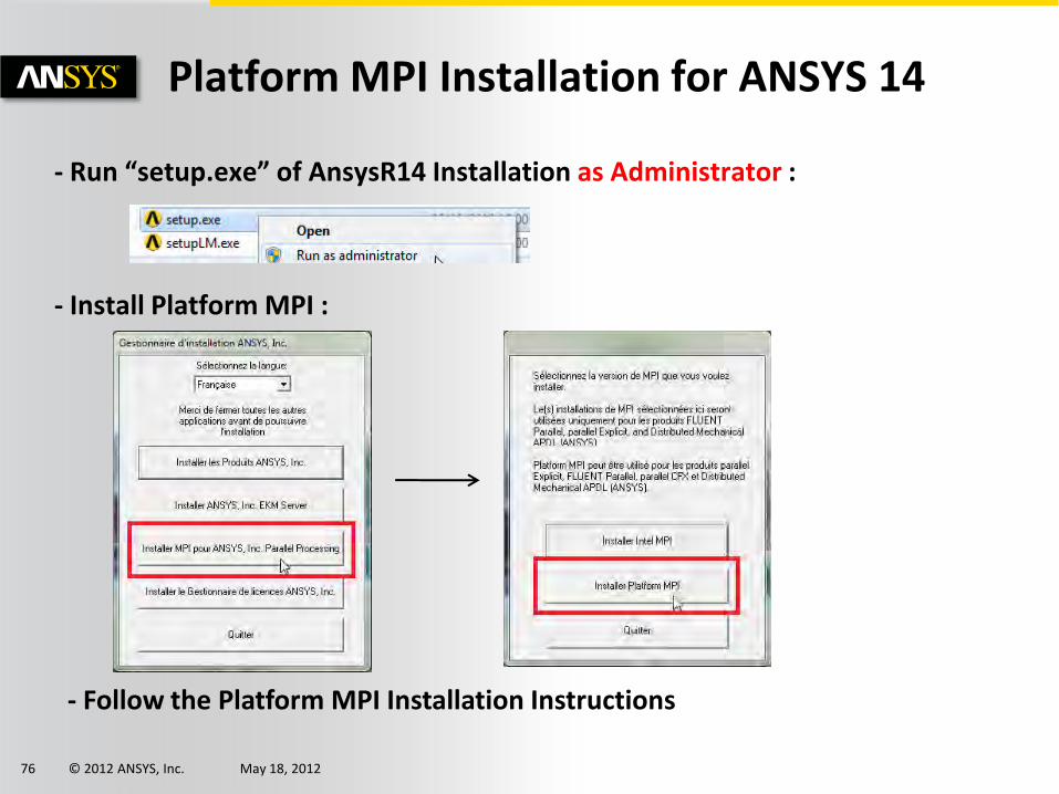
Platform MPI Installation for ANSYS 14
- Run “setup.exe” of AnsysR14 Installation as Administrator :
- Install Platform MPI :
- Follow the Platform MPI Installation Instructions
© 2012 ANSYS, Inc. May 18, 2012 77
Platform MPI Installation for ANSYS 14
For ANSYS Mechanical customers who have R13 installed and wish to continue to use R13, please run the following command to ensure compatibility :
"%AWP_ROOT140%\commonfiles\MPI\Platform\8.1.2\Windows\HPMPICOMPAT\hpmpicompat.bat“
(by default : “C:\Program Files\ANSYS Inc\v140\commonfiles\MPI\Platform \8.1.2\Windows\HPMPICOMPAT\hpmpicompat.bat”)
The command will display a dialog box with a title of "ANSYS 13.0 SP1 Help".
Note for ANSYS Mechanical R13 users
© 2012 ANSYS, Inc. May 18, 2012 78
Platform MPI Installation for ANSYS 14
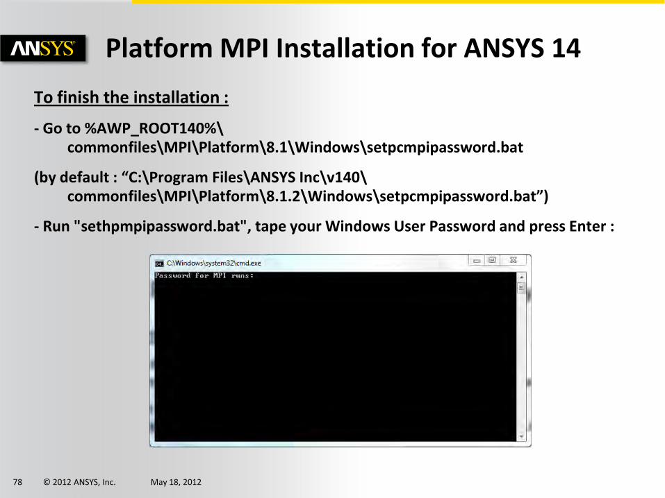
To finish the installation :
- Go to %AWP_ROOT140%\ commonfiles\MPI\Platform\8.1\Windows\setpcmpipassword.bat
(by default : “C:\Program Files\ANSYS Inc\v140\ commonfiles\MPI\Platform\8.1.2\Windows\setpcmpipassword.bat”)
- Run "sethpmpipassword.bat", tape your Windows User Password and press Enter :
© 2012 ANSYS, Inc. May 18, 2012 79
Test MPI Installation for ANSYS 14
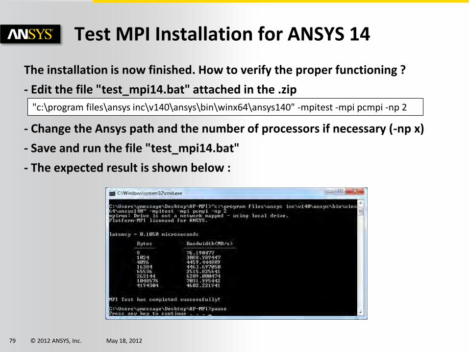
The installation is now finished. How to verify the proper functioning ?
- Edit the file "test_mpi14.bat" attached in the .zip
- Change the Ansys path and the number of processors if necessary (-np x)
- Save and run the file "test_mpi14.bat"
- The expected result is shown below :
"c:\program files\ansys inc\v140\ansys\bin\winx64\ansys140" -mpitest -mpi pcmpi -np 2
© 2012 ANSYS, Inc. May 18, 2012 80
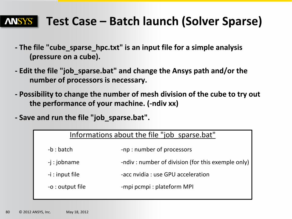
Test Case – Batch launch (Solver Sparse)
- The file "cube_sparse_hpc.txt" is an input file for a simple analysis (pressure on a cube).
- Edit the file "job_sparse.bat" and change the Ansys path and/or the number of processors is necessary.
- Possibility to change the number of mesh division of the cube to try out the performance of your machine. (-ndiv xx)
- Save and run the file "job_sparse.bat".
Informations about the file "job_sparse.bat"
-b : batch -np : number of processors
-j : jobname -ndiv : number of division (for this exemple only)
-i : input file -acc nvidia : use GPU acceleration
-o : output file -mpi pcmpi : plateform MPI
© 2012 ANSYS, Inc. May 18, 2012 81
Test Case – Batch launch (Solver Sparse)
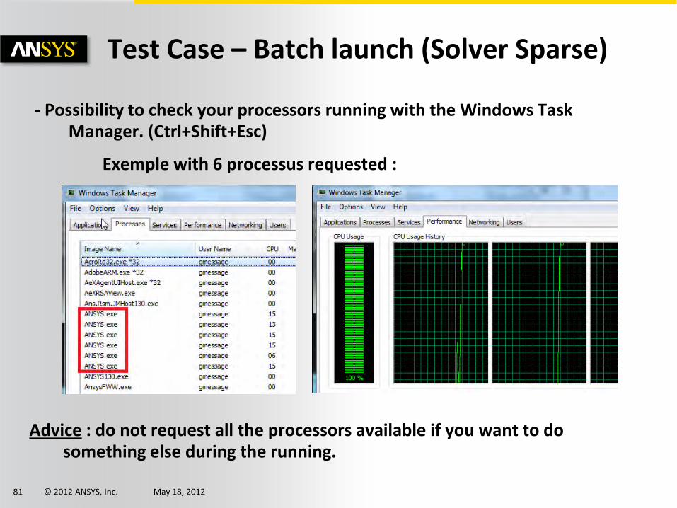
- Possibility to check your processors running with the Windows Task Manager. (Ctrl+Shift+Esc)
Exemple with 6 processus requested :
Advice : do not request all the processors available if you want to do something else during the running.
© 2012 ANSYS, Inc. May 18, 2012 82
Test Case – Batch launch (Solver Sparse)
Once the running is finished :
- Read the file .out to collect all the informations about the solver output.
- The main informations are :
- Elapsed Time (sec)
- Latency Time from Master to core
- Communication Speed from Master to core
- Equation solver computational rate
- Equation solver effective I/O rate
© 2012 ANSYS, Inc. May 18, 2012 83
Test Case – Workbench launch
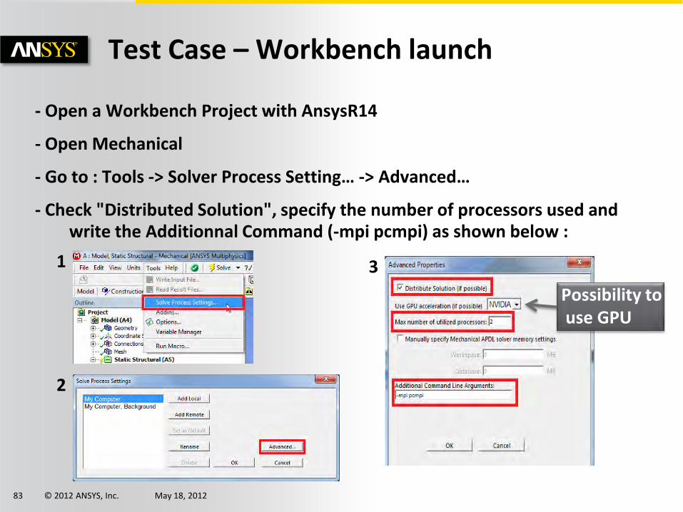
- Open a Workbench Project with AnsysR14
- Open Mechanical
- Go to : Tools -> Solver Process Setting… -> Advanced…
- Check "Distributed Solution", specify the number of processors used and write the Additionnal Command (-mpi pcmpi) as shown below :
2
1 3
Possibility to use GPU
© 2012 ANSYS, Inc. May 18, 2012 84
Test Case – Workbench launch
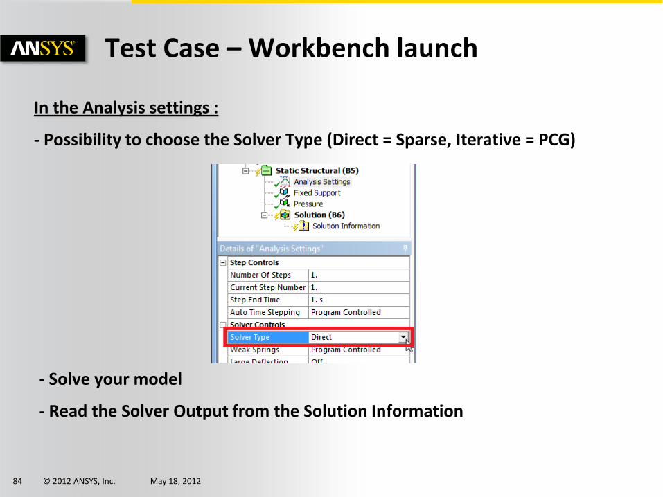
In the Analysis settings :
- Possibility to choose the Solver Type (Direct = Sparse, Iterative = PCG)
- Solve your model
- Read the Solver Output from the Solution Information
© 2012 ANSYS, Inc. May 18, 2012 85
Automated run for a model
Compare customer results with ANSYS reference
First step for an HPC test on customer machine
Appendix
© 2012 ANSYS, Inc. May 18, 2012 86
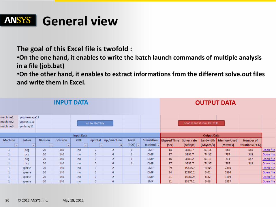
General view
INPUT DATA OUTPUT DATA
The goal of this Excel file is twofold : •On the one hand, it enables to write the batch launch commands of multiple analysis in a file (job.bat) •On the other hand, it enables to extract informations from the different solve.out files and write them in Excel.
© 2012 ANSYS, Inc. May 18, 2012 87
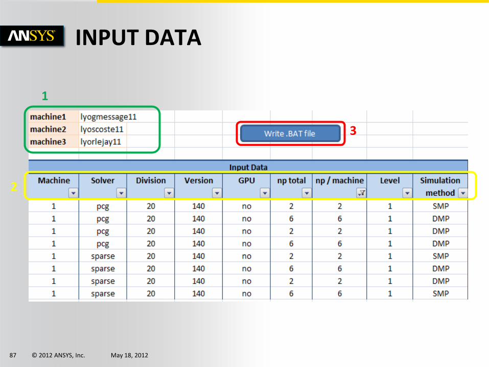
INPUT DATA
1
2
3
© 2012 ANSYS, Inc. May 18, 2012 88
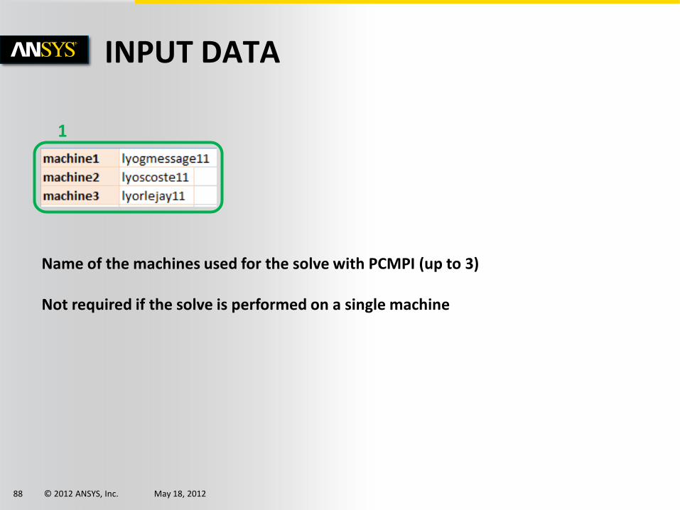
INPUT DATA
1
Name of the machines used for the solve with PCMPI (up to 3) Not required if the solve is performed on a single machine
© 2012 ANSYS, Inc. May 18, 2012 89
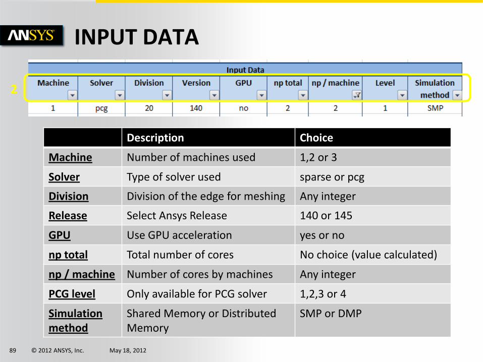
INPUT DATA
Description Choice
Machine Number of machines used 1,2 or 3
Solver Type of solver used sparse or pcg
Division Division of the edge for meshing Any integer
Release Select Ansys Release 140 or 145
GPU Use GPU acceleration yes or no
np total Total number of cores No choice (value calculated)
np / machine Number of cores by machines Any integer
PCG level Only available for PCG solver 1,2,3 or 4
Simulation method
Shared Memory or Distributed Memory
SMP or DMP
2
© 2012 ANSYS, Inc. May 18, 2012 90
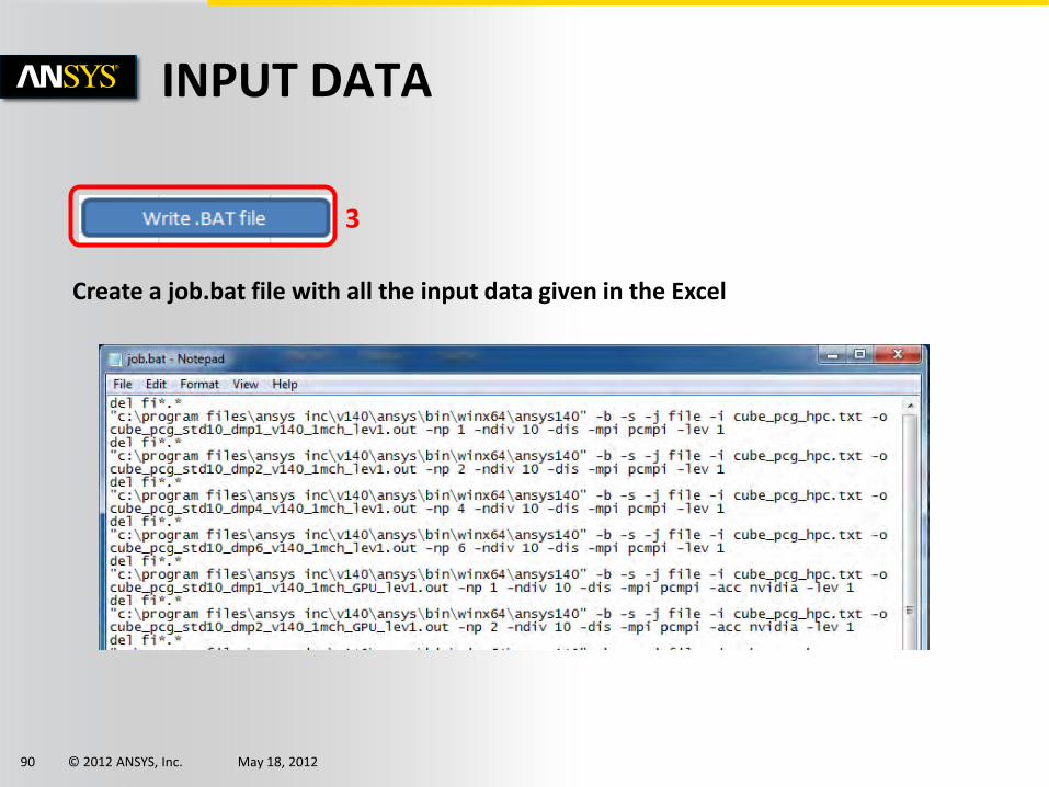
INPUT DATA
3
Create a job.bat file with all the input data given in the Excel
© 2012 ANSYS, Inc. May 18, 2012 91
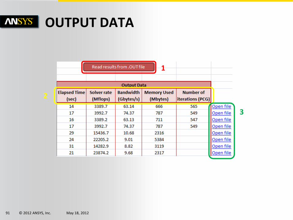
OUTPUT DATA
1
2
3
© 2012 ANSYS, Inc. May 18, 2012 92
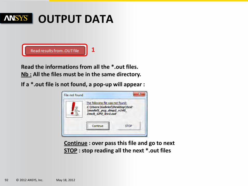
OUTPUT DATA
1
Read the informations from all the *.out files. Nb : All the files must be in the same directory.
If a *.out file is not found, a pop-up will appear :
Continue : over pass this file and go to next STOP : stop reading all the next *.out files
© 2012 ANSYS, Inc. May 18, 2012 93
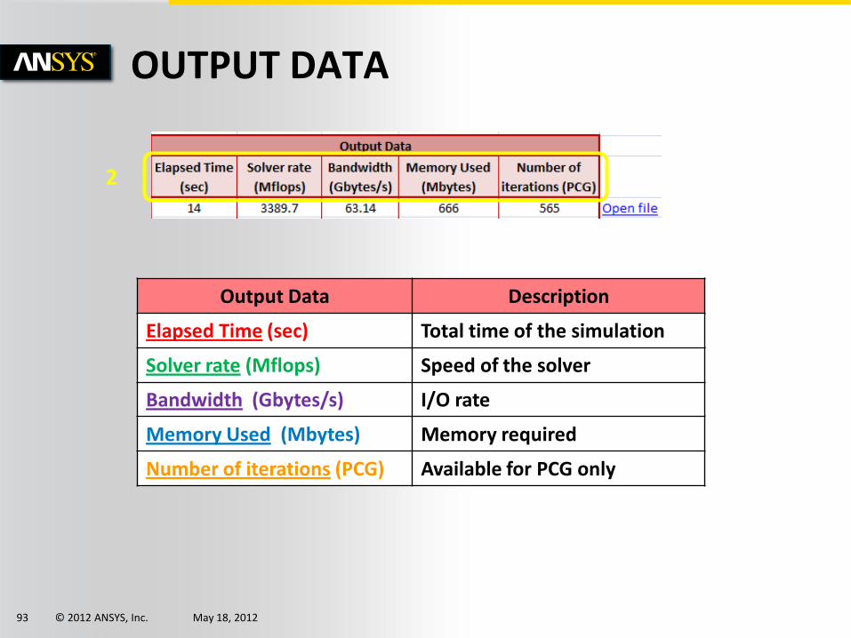
OUTPUT DATA
2
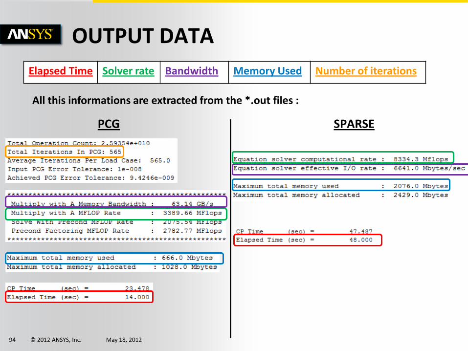
Output Data Description
Elapsed Time (sec) Total time of the simulation
Solver rate (Mflops) Speed of the solver
Bandwidth (Gbytes/s) I/O rate
Memory Used (Mbytes) Memory required
Number of iterations (PCG) Available for PCG only
© 2012 ANSYS, Inc. May 18, 2012 94
OUTPUT DATA
All this informations are extracted from the *.out files :
Elapsed Time Solver rate Bandwidth Memory Used Number of iterations
PCG SPARSE
© 2012 ANSYS, Inc. May 18, 2012 95
OUTPUT DATA
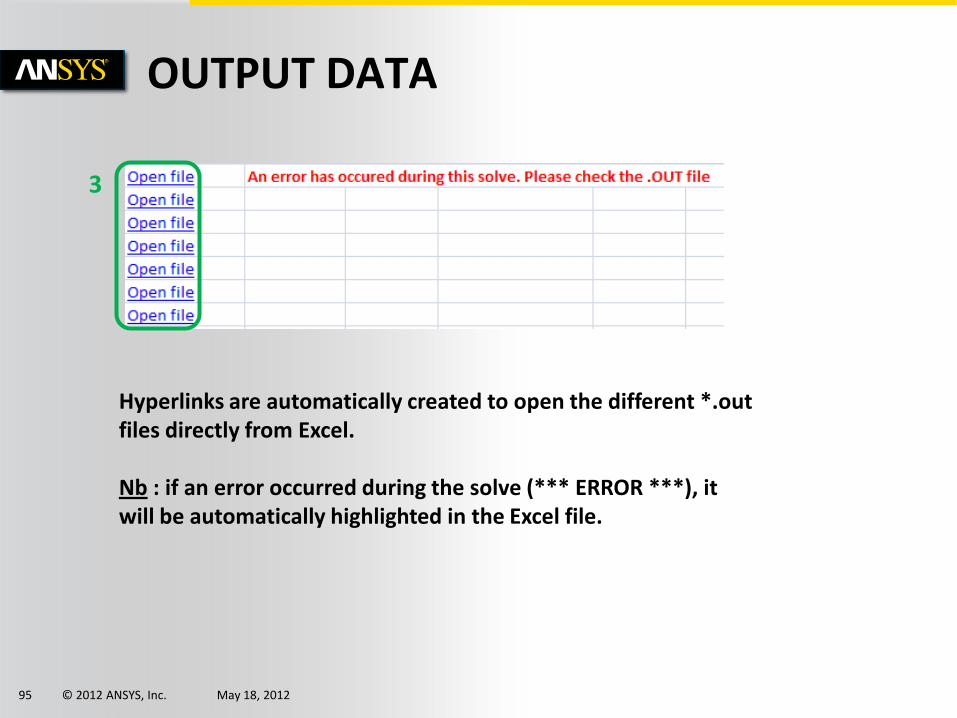
3
Hyperlinks are automatically created to open the different *.out files directly from Excel. Nb : if an error occurred during the solve (*** ERROR ***), it will be automatically highlighted in the Excel file.

© 2012 ANSYS, Inc. May 18, 2012 96
And now : waiting your feedback ,
from your results
© 2012 ANSYS, Inc. May 18, 2012 97
Any suggestion/question for Excel tool improvement :
© 2012 ANSYS, Inc. May 18, 2012 98
THANK YOU