h.p. williams london school of economics models for solving the travelling salesman problem...
TRANSCRIPT

H.P. WILLIAMS
LONDON SCHOOL OF
ECONOMICS
MODELS FOR SOLVING
THE
TRAVELLING SALESMAN PROBLEM

STANDARD FORMULATION OF THE (ASYMMETRIC) TRAVELLING
SALESMAN PROBLEM
Conventional Formulation:
(cities 1,2, …, n) (Dantzig, Fulkerson, Johnson) (1954). is a link in tour
Minimise:
subject to:
ji
ijijxc
,
}...,{,
nSSxijSji
2 all 1 - | |
1 all ijj
x i
1 all iji
x j
ijx

62
3
e.g.
632632 xxx
2366223 xxx
0(2n) Constraints = (2n-1 + n –2) 0(n2) Variables = n(n – 1)

EQUIVALENT FORMULATION
Replace subtour elimination constraints with
1
SjSi
ijx all nS ,...,,2,1
____
S
S
Add second set of constraints for all i in S and subtract from subtour elimination constraints for S

OPTIMAL SOLUTON TO A 10 CITY TRAVELLING SALESMAN PROBLEM
10
1
8 6
3
2
7
9
5
4
Cost = 881

FRACTIONAL SOLUTION FROM CONVENTIONAL (EXPONENTIAL)
FORMULATION)
Cost = 878 (Optimal Cost = 881)

Sequential Formulation (Miller, Tucker, Zemlin (1960))
ui = Sequence Number in which city i visited
Defined for i = 2,3, …, nSubtour elimination constraints replaced by
S: ui - uj +nxij n – 1 i,j = 2,3, …, n
Avoids subtours but allows total tours (containing city 1)
62
3
Weak but can add 'Logic Cuts'
u2 – u6+ nx26
n-1
u6 – u3+ nx63
n-1
u3 – u2+ nx32
n-1 3n 3(n – 1)
0(n2) Constraints = (n2 – n + 2)0(n2) Variables = (n – 1) (n + 1)
e.g. 11k ij jk ju x x x

FRACTIONAL SOLUTION FROM SEQUENTIAL FORMULATION
Subtour Constraints Violated : e.g.
Logic Cuts Violated: e.g.
Cost = 773 3/5 (Optimal Cost = 881)
17227 xx
17792791 xxxu

Flow Formulations
Single Commodity (Gavish & Graves (1978)) Introduce extra variables (‘Flow’ in an arc) Replace subtour elimination constraints by
F1:
1 all 1
1
, all )1(
1
jyy
ny
jixny
kjk
iij
jj
ijij
Can improve (F1’) by amended constraints:
ijijxny )2(
1, jiall

Network Flow formulation in variables over complete graph
ijy
4
2
1
3 1
1 1
Graph must be connected. Hence no subtours possible.
Constraints Variables
)(0 2n )2( nn
)(0 2n )1(2 nn
n-1

FRACTIONAL SOLUTION FROM SINGLE COMMODITY FLOW FORMULATION
Cost = 794 (Optimal solution = 881) 2
9

FRACTIONAL SOLUTION FROM MODIFIED SINGLE COMMODITY FLOW FORMULATION
Cost = (Optimal solution = 881) (192=3x64)
48
43794
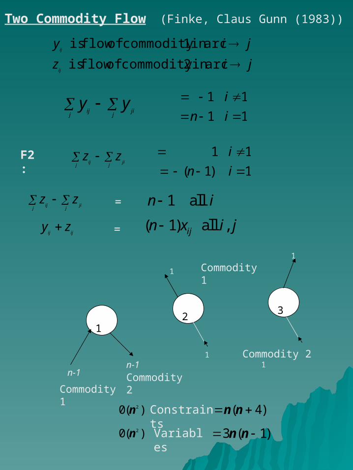
Two Commodity Flow (Finke, Claus Gunn (1983))
jiz
jiy
ij
ij
arcin 2commodity of flow is
arcin 1commodity of flow is
j
jij
ijyy
11
11
in
i
j
jij
ijzz
1)1(
11
in
i
j
jij
ijzz 1 all n i
ijijzy ( 1) all ,ijn x i j
=
=
F2:
1 2
3
1
1
1 Commodity 2 1
)(0 2n )4( nn
)(0 2n )1(3 nnVariables
Constraints
n-1
Commodity 1Commodity 2n-1
Commodity 1

Multi-Commodity (Wong (1980) Claus (1984)) “Dissaggregate” variables
k
ijy is flow in arc destined
for k
i, j, kxyij
k
ij all
k all001111
j
k
kji
k
ii
k
ii
k
ikyyyyF3
.,1,, all kjjkjyyi
k
jii
k
ij
)(0 3n 362 23 nnn
)(0 3n 12 nn Variables
Constraints
LP Relaxation of equal strength to Conventional Formulation. But of polynomial size. Tight Formulation of Min Cost Spanning Tree + (Tight) Assignment Problem

FRACTIONAL SOLUTION FROM MULTI COMMODITY FLOW FORMULATION (=
FRACTIONAL SOLUTION FROM CONVENTIONAL (EXPONENTIAL) FORMULATION)
Cost = 878 (Optimal Cost = 881)

Stage Dependent Formulations First (Fox, Gavish, Graves (1980))
= 1 if arc traversed at stage t
= 0 otherwise T1:
ji
nytji
t
ij
,,
n...3,211121
itytyn
t
t
ji
n
j
n
t
t
ij
n
j
1,0
1,0
,0
1
1
1
iy
ty
nty
ij
t
j
t
i
1Variables0
sConstraint023
nnn
nn
(Stage at which i left 1 more than stage at which entered)
t
t
ijijyx
Also convenient to introduce ijx variables with constraints

FRACTIONAL SOLUTION FROM 1ST (AGGREGATED) TIME-STAGED FORMULATION
Cost = 364.5 (Optimal solution = 881)
NB ‘Lengths’ of Arcs can be > 1

1,
tij
tji
y
1,
tij
tij
y
Second (Fox, Gavish, Graves (1980))
T2: Disaggregate to give
all j
all i
all t
nityty tji
n
t
tij
n
t
n
j
... ,3,2 1 - 1
n
1j21
Initial conditions no longer necessary
0(n) Constraints = 4 n – 1
0(n3) Variables = n2 (n – 1)
1,,
tij
jiji
y

FRACTIONAL SOLUTION FROM 2nd TIME-STAGED FORMULATION
Cost =164
799357
(optimal solution = 881)
(714 = 2 x 3 x 7 x 17)

Third (Vajda/Hadley (1960))
T3:
tijy interpreted as
before 1
tij
ji
y all j
1
tij
ij
y all i
1 tij
t
y all t
t
ijji
y
1
t
jkjk
y= 0 all j, t
11
1j
j
y
= 1
ni
i
y 11
= 1
0 (n2) Constraints = (2n2+ 3)
0 (n3) Variables = n2(n-1)

FRACTIONAL SOLUTION FROM 2nd TIME 2nd TIME-STAGED FORMULATION
Cost =1
8042
Optimal solution = 881
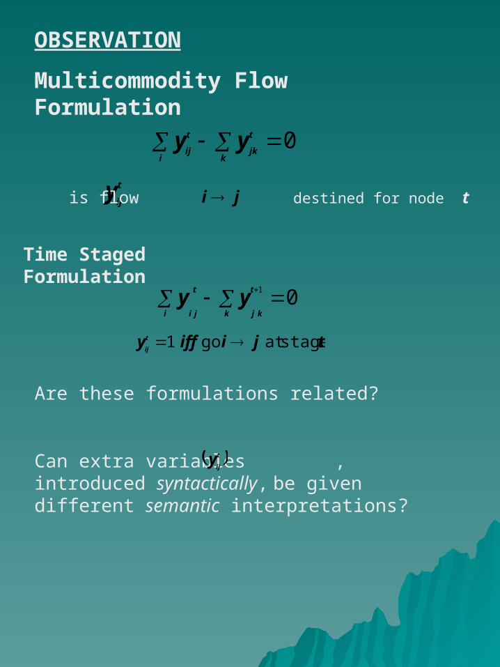
OBSERVATION
Multicommodity Flow Formulation
0k
t
jki
t
ijyy
t
ijy ji is flow destined for node t
Time Staged Formulation
01
t
kjk
t
jii
yy
tjiiffy t
ij stageat go1
Are these formulations related?
Can extra variables , introduced syntactically, be given different semantic interpretations?
t
ijy

COMPARING FORMULATIONS
Minimise:
c x
Subject to:
bByAx integer ,0 , xyx
}0,0|{ wwBwW
W forms a cone which can be characterised by its extreme rays
giving matrix Q such that 0QB
QbQAx Hence
ijx
This is the projection of formulation into space of original variables

COMPARING FORMULATIONS
Project out variables by Fourier-Motzkin elimination to reduce to space of conventional formulation.
P (r) is polytope of LP relaxation of projection of formulation r.
Formulation S (Sequential)
Project out around each directed cycle S by summing
1 nnxuuijji
SnxnSji
ij1
,
ie n
SSx
Sjiij
,
weaker than |S|-1 (for S asubset of nodes)
Hence CPSP

Formulation F1 (1 Commodity Network Flow)
n
|| - |S|han stronger t
1
||||
S
n
SSxij
sij
Projects to
)()1()( CPFPSP Hence
Formulation F1' (Amended 1 Commodity Network
Flow)
1
||||
1
1
,}1{
n
SSxx
n ijSji
ij
SjSj
Projects to
Hence )()'1()1()( CPFFFPSP
Formulation F2 (2 Commodity Network Flow)
Projects to 1
||||
, n
SSxij
ji
Hence P(F2) = P(F1)

Formulation F3 (Multi Commodity Network Flow)
Projects to 1||
,
Sx ij
Sji
Hence P(F3) = P(C)
Formulation T1 (First Stage Dependant)
Projects to
1
||
}1{
n
Sxij
SjSi
nxNji
ij ,
5, ji
ijx(Cannot convert 1st constraint to ‘ ‘form since
Assignment Constraints not present)

Formulation T2 (Second Stage Dependant)
Projects to
1
||||
1
1
1
1}1{
}1{
n
SSxx
nx
n sijjijij
SjSi
ij
SjSi
Hence P(T2) P(F1')
+ others
Formulation T3 (Third Stage Dependant)
Projects to
1
||||
1
1
1
1,}1{
}1{
n
SSxx
nx
n Sjnijij
SjSi
ij
SjSi
+ others
Can show stronger than T2
Hence P(T3) P(T2)

M o d e l S iz e L P O bj
I t s S e c s I P O bj
N o d e s S e c s
C (C on v en tion al
502x90 (A ss. R elax +Su btou rs (5) +Su btou rs (3) +Su btou rs (2)
766 804 835 878
37 40 43 48
1 1 1 1
766 804 835 881
0 0 0 9
1 1 1 1
S (Sequ en tial )
92x99 773.6 77 3 881 665 16
F 1 1(C om m od i ty F low
F ' (F 1 M od ifi ed )
120x180
120x180
794.22
794.89
148
142
1
1
881
881
449
369
13
11
F 2 (2 C om m od i ty F low )
140x270 794.22 229 2 881 373 12
F 3 (M u l ti
C om m od i ty F low )
857x900 878 1024 7 881 9 13
T 1 (1st Stage
D ep en d en t)
90x990 (10)x(900)
364.5 63 4 881
T 2 (2n d Stage D ep en d en t)
120x990 (39) x (900)
799.46 246 18 881 483 36
T 3 (3rd Stage
D ep en d en t)
193x990 (102)x(900)
804.5 307 5 881 145 27
Computational Results of a 10-City TSP in order to compare sizes and strengths of LP Relaxations
Solutions obtained using NEW MAGIC and EMSOL

P(TSP) TSP Polytope – not fully known
P(X) Polytope of Projected LP relaxations

ReferenceReference
AJ Orman and HP Williams,AJ Orman and HP Williams,
A Survey of Different Formulations of the A Survey of Different Formulations of the Travelling Salesman Problem, Travelling Salesman Problem,
in C Gatu and E Kontoghiorghes (Eds),in C Gatu and E Kontoghiorghes (Eds), Advances in Computational Management Advances in Computational Management Science 9 Optimisation, Econometric and Science 9 Optimisation, Econometric and Financial Analysis (2006) SpringerFinancial Analysis (2006) Springer