UCRL- JC-121239 PREPRINT

The Effects of Elevation Data Representation on Mesoscale Atmospheric Model Simulations

Hoyt Walker John Leone

Jimwon Kim Atmospheric & Ecological Sciences

Lawrence Livermore National Laboratory

Presented to: 3rd International ConferenceJWorkshop on

Integrating GIs and Environmental Modeling Sante €e, New Mexico, January 21 -25,1996

Thisis apreprintof apaperintendedforpublicationina joumalorproceedings. Since changes may be made before publication, this preprint is made available with the understanding that it will not be cited or reproduced without the permission of the author.

7

~

FEB 0 6 1996 O S T t

A

DISCLAIMER

This document was prepared as an account of work sponsored by an agency of the United States Government. Neither the United States Government nor the University of California nor any of their employees, makes any warranty, express or implied, or assumes any legal liability or responsibility for the accuracy, completeness, or usefulness of any information, apparatus, product, or process disclosed, or represents that its use would not infringe privately owned rights. Reference herein to any specific commercial product, process, or service by trade name, trademark, manufacturer, or otherwise, does not necessarily constitute or imply its endorsement, recommendation, or favoring by the United States Government or the University of California. The views and opinions of authors expressed herein do not necessarily state or reflect those of the United States Government or the University of California, and shall not be used for advertising or product endorsement purposes.

Portions of this document may be illegible in electronic image products. Smages are produced from the best avabble original dorlrment.

UCRL-JC-121239

The Effects of Elevation Data Representation on Mesoscale Atmospheric Model Simulations

Hoyt Walker, John M. Leone, Jr. and Jinwon Kim Lawrence Livermore National Laboratory

P.O. Box 808 Livermore, CA 9455 1-0808

Fax: (510) 423-4527 (5 10) 422- 1840

ABSTRACT Mesoscale atmospheric model simulations rely on descriptions of the land surface characteristics, which must be developed from geographic databases. Certain features of the geographic data, such as its resolution and accuracy, as well as the method of processing for use in the model, can be very important in producing accurate model simulations. The work described here is part of research effort into the relationship between these aspects of geographic data and the performance of mesoscale atmospheric models and is particularly focused on elevation data and how it is prepared for use in such models.

A source for digital elevation data will typically not be at the resolution required for a given model simulation and so a resampling step is required. In addition, predictive non-linear model often cannot accept forcing at high spatial frequencies due to the terrain, thus smoothing is also required. The effect of different means of resampling and smoothing elevation data on two types of model simulations is investigated. At smaller spatial scales, nocturnal drainage winds in mountain valleys in Colorado are examined for effects on the general characteristics as well as the details of the flows. At the larger end of the mesoscale, extended simulations of California weather are examined for effects on orographic lifting, low-level convergence and divergence and ultimately rain and snow distribution.

INTRODUCTION In mesoscale atmospheric modeling, a variety of surface features such as the elevation, surface roughness, and sensible and latent heat fluxes must be represented in the model (Pielke, 1984; Lee, et.al., 1991). These features, expressed in the form of model boundary conditions, must be developed from geographical databases in a way that balances the need for descriptive detail and accuracy with the spatial discretization of a specific model simulation. This is due to both the physics and numerical techniques in a model and to the close coupling of the land surface with boundary layer phenomena under many conditions [Pielke, 19841. This paper focuses specifically on elevation data and how it is processed for use in an atmospheric model. Because of its static nature, it forms a convenient starting point for looking at the interaction between geographic data and atmospheric models. Before describing the details of the research presented in this paper, it is appropriate to provide some background on the use of elevation data in regional atmospheric models.

Elevation data representation in mesoscale atmospheric models. Defining the shape of the lower boundary of an atmospheric model domain using elevation data is clearly an essential component for explicit modeling of the atmospheric boundary layer given the need to represent the steering and lifting effects of the elevation surface, as well as to model the variable surface heating due spatial variations in terrain slope and aspect. There are a variety of ways of defining the elevation surface in a model, which for mesoscale models involves defining the elevations at the horizontal grids points of the model (global models often solve their governing equations in spectral space and consequently descretize spectral space, in contrast, mesoscale models are essentially always expressed in physical space with model variables tracked on a three-dimensional grid). For example, triangular or rectangular grids can be used. Although research into triangular grids is on-going [see Boybeyi, et.al., 19941, virtually all mesoscale models in common use rely on rectangular grids. Terrain representations can also be classified into stepped and continuous representations. In stepped terrain, the landform is approximated by stacks of building blocks or tiles that represent some average elevation over a model grid cell, while in a continuous representation, the elevations are defined at horizontal grid points and some interpolation scheme, e.g., bilinear, can be assumed to define a continuous surface at all x,y locations in the model grid. These approaches are illustrated in Figure 1 for two dimensions. The National Weather Service Eta model uses a stepped terrain representation operationally to perform weather prediction for North America [Mesinger, et& 19881. As most mesoscale atmospheric models use some form of continuous terrain representation, this paper concentrates on models that use rectangular grids and continuous terrain representations.

Elevation data has a particularly critical role in most mesoscale models, not only because it defines the shape of the lower boundary but the landform also affects the spatial discretization throughout much of the grid volume as shown in Figure la. This is because such models typically incorporate some form of terrain-following coordinate system where the terrain surface is defined as one limit of a transformed vertical coordinate (e.g., 0) and the top of the model domain is defined as the other limit (e.g., 1). In physical coordinates, the grid points are compressed and stretched as the terrain rises and falls, again as shown in Figure la. Thus the landform not only affects the details of the surface interactions, but it also affects the geometry of the grid above the surface. Therefore, the manner in which the terrain is represented can have effects on the numerical representation of the flow throughout much of the grid. Also, shown in Figure la is a graded (or stretched) vertical grid, where there is a greater density of grid points near the land surface and fewer points near the grid top. Given the complexity of the physical processes just above the land surface and their relatively small length scale, using greater resolution near the ground is usually necessary in mesoscale models that explicitly model the behavior of the planetary boundary layer.

An important constraint on prognostic model representations of terrain is related to stable performance through simulated time of such models. Forcing a non-linear prognostic model at high spatial frequencies relative to the model grid step (i.e. variation with wavelengths of 2-4Ax, where Ax is the length of a model grid step) can destabilize model performance, which can result in the exponential buildup of high-frequency waves that swamp the realistic aspects of the simulation. Winds blowing over terrain with significant 2-4Ax variation represents a constant high frequency forcing of the model that can limit the accuracy of the simulation. As a result, the model elevations are typically smoothed to avoid this problem. A related issue involves the parameterization of subgrid scale terrain variation. Any roughness on the earth’s surface acts as a momentum sink and thus affects the atmospheric flow. The elevation surface in the model can only represent and explicitly model the effects of terrain variation with wavelengths of 2Ax and longer. Unresolved terrain variation is can be parameterized by adjusting the surface roughness height, which is normally used to express the effect on the flow of surface elements such as grass, trees and buildings (see, for example,. Georgelin, et.al., 1994; Mason, 1991). Another important aspect of terrain representation is associated with the barrier that a range of hills or mountains presents to an atmospheric flow across it. A number of important atmospheric phenomena are strongly affected by the height of such a barrier, e.g., lee cyclogenesis and orographic precipitation. Problems can occur with a terrain representation that relies on a simple mean to represent the barrier height if the model grid step is large with respect to the horizontal scale of significant relief. Mean elevations tend to lower the maximum heights, which can alter the effective barrier height for the flow. At synoptic and larger scales, mean elevations are often modified by adding a factor (typically 1 or 2) times the standard deviation of the terrain. Such a surface is called an envelope terrain and it raises the effective barrier and produces better model simulations (Tibaldi, 1986; Wallace, et.al., 1983). These examples illustrate the need to consider the physics, the numerics and the application in determining how to most effectively representation geographic data in an atmospheric model.

This research focuses on two aspects of elevation data representation in mesoscale atmospheric models. First, the sensitivity of small-scale model simulations of nocturnal drainage winds to the smoothness and variability of the elevation data representation is examined The development of nocturnal drainage winds is one example of a terrain driven atmospheric flow and offers a useful test case for examining the effects of elevation data on mesoscale models (Leone & Lee, 1989). In earlier work, a number of model simulations using idealized terrain have been performed and analyzed (Walker & Leone, 1994). Here we extend the investigation by conducting a series of model experiments to determine the response of a hydrostatic mesoscale atmospheric model to lower boundary forcing due to variations in the representation of a real mountain valley system during nocturnal cooling.

Second, the effective of different resampling techniques on a regional-scale simulation focused on the distribution of precipitation is considered. There are numerous ways resampling elevation data for regional models that are intended to resolve primarily sub-synoptic scale motions. Perhaps the most common way is to use a grid cell mean terrain computed from fine resolution elevation data. As suggested by the synoptic scale work mentioned above, the orographic effects of a mountain barrier can sometimes be improved using an envelope terrain, which can differ substantially from the mean terrain in mountainous regions. For mesoscale motions, the terrain affects the atmospheric flow through orographically-generated vertical motion and local convergence, which ultimately affect low-level wind and transport of tracers, such as water vapor, associated with the low-level wind. The effects of using these two approaches to creating a terrain representation will be examined here.

For historical reasons, these two aspects of this study have been performed using different mesoscale models. As a result, the rest of the paper will be structured into sections covering the small-scale effects, followed by a section

covering the regional-scale effects. The results of both sections will be summarized in the conclusion.

SMALL-SCALE EFFECTS In this study, a basic drainage flow is defined along the Brush Creek valley system in western Colorado, the site of the ASCOT field experiments (see Clements et.al., 1989), using a mesoscale atmospheric model relying unsmoothed elevation data to define the lower boundary (for this particular situation, unsmoothed elevation data does not cause problems with the stability of the simulation). The elevation data is then altered in various ways and used as the basis for additional simulations. Some specific details of the control simulation and one comparison run are described in the following sections.

Model Description The atmospheric model used in these tests is called SABLE (Simulator of the Atmospheric Boundary Layer Environment), a hydrostatic mesoscale model developed at the Lawrence Livermore National Laboratory. SABLE solves the hydrostatic, anelastic, equations for velocity, potential temperature, and Exner function in three dimensions (Zhong, et.al. 1991). The equations are solved by using a unique blend of numerical techniques. The prognostic equations for the horizontal velocity components and the potential temperature are solved using trilinear, isoparametric finite elements in space combined with a semi-implicit time integration scheme. The diagnostic equations for vertical velocity and Exner function are solved by integrating up or down vertical columns, respectively, via centered finite differences. Turbulence was modeled using the local Richardson numberdependent K model of McNider and Pielke (1981).

Model Domain For all simulations, a horizontal grid was used that covers a 7 by 32 km area oriented along Brush Creek with a 200 m grid step, , i.e., the grid had 36 by 161 nodes in the horizontal directions (see Figure 2). The domain also includes a portion of the valley into which Brush Creek drains (Roan Creek). The horizontal coordinate system was derived from the Universal Transverse Mercator (UTM) projection for this area using a translation and 45 degree rotation to align the y axis with the centerline of Brush Creek. The upper boundary of the domain was is flat at an altitude of 4000 m (the minimum and maximum elevations in the grid for the unsmoothed terrain are 1650 and 2650 m, respectively). The vertical grid was graded with the lowest cell being 20 m.

The lower boundary of the domain was defined using elevation data extracted from a Defense Mapping Agency @MA) Digital Terrain Elevation Data (DTED) quadrangle covering the Brush Creek area at 3 arc-second resolution. The raw elevation data was resampled to the model grid using an unweighted mean. The smoothed terrain was generated by using a 9 by 9 binomial filter data with only the original data used at each step in computing the weighted average to avoid propagation effects (see Figure 2b). Elevations beyond the model grid boundary were accessed to create a buffer regional so that the filter stencil could extend beyond the model grid without using an artificial boundary condition. Sine waves were added to the valley floor and sides for two of the runs with the waves diminishing to zero as the valley ridges were approached. The magnitudes of the sine waves were 40 m and two wavelengths were used, 4Ax and 8Ax (see Figures 2c and 2d).

Initialization Given the goal of isolating the effects of terrain representation on a model run, accurately reproducing any particular physical situation was not of great importance. Thus, a number of simplifying assumptions were made. For example, the Coriolis parameter was set to zero to avoid complicated veering motions. The cross-side valley wind component, u, was assumed to be zero at the appropriate lateral boundaries. At the top boundary, both horizontal wind components, u and v, were set to zero. The lower boundary cooling was specified as a heat flux of -60 W/ mz . The atmosphere was initialized to be slightly stable with a potential temperature lapse rate of 0.002 Wm. The problems were run for 8 hours. These values were used in all of the runs, thus, the only differences between simulations were the elevation surfaces.

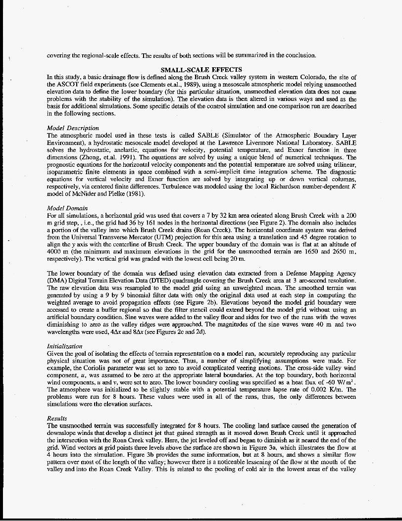
Results The unsmoothed terrain was successfully integrated for 8 hours. The cooling land surface caused the generation of downslope winds that develop a distinct jet that gained strength as it moved down Brush Creek until it approached the intersection with the Roan Creek valley. Here, the jet leveled off and began to diminish as it neared the end of the grid. Wind vectors at grid points three levels above the surface are shown in Figure 3a, which illustrates the flow at 4 hours into the simulation. Figure 3b provides the same information, but at 8 hours, and shows a similar flow pattern over most of the length of the valley; however there is a noticeable lessening of the flow at the mouth of the valley and into the Roan Creek Valley. This is related to the pooling of cold air in the lowest areas of the valley

system. The variation of the maximum down-valley wind component along the valley is summarized in Figure 3c.

The smoothed terrain simulation shows the same general characteristics as the unsmoothed terrain; however, the flow over the smoothed terrain is distinctly stronger. For example, the maximum speed along the length of the valley increases from 5.8 to 7.2 mls at 4 hours between the two runs while the maximum speed at 8 hours increases from 5.6 to 6.8 d s . This is also apparent when the down-valley speed maximum for the smoothed and unsmoothed terrains are compared (see Figures 4a and 3c). Of particular interest is the change in the counterflow that occurs between these two runs. In addition to the main jet that forms in the valley, a counterflow also develops above the valley over the entire width of the domain for all the simulations. This counterflow changes significantly with the altered surface representations (see Figure 5) with the unsmoothed terrain having the strongest counterflow. The addition of waves to the smoothed terrain weakens the counterflow relative to the smoothed terrain as well as effecting the details of the jet as it flows over the waves. As the counterflow builds up between 4 and 8 hours into the simulation it tends to confine the jet within the valley walls

REGIONAL-SCALE EFFECTS In this study, a winter storm in California is simulated using a primitive-equation, limited-area model with particular attention being focused on the distribution and intensity of precipitation in this area. The effects of two different terrain representations on the simulated low-level wind and precipitation and examined. The commonly used mean terrain representation provides the control case and a 1-sigma envelope provides a comparison simulation.

Model description Details of the dynamical and physical formulations of the Mesoscale Atmospheric Simulation (MAS) model have been presented by Kim and Soong (1994) and Soong and Kim (1995). In summary, the governing equations of the MAS model are the flux-form of the primitive equations written in o-coordinates and discretized on Arakawa c-grid. The advection of momentum is computed using a thiid-order accurate scheme by Takacks (1985) with the advection of the remaining dependent variables computed by a finite difference scheme by Hsu and Arakawa (1990). Vertical staggering and differencing of variables follow the formulation by Arakawa and Suarez (1983).

Precipitation processes are computed separately for deep convection and grid-scale condensation using the Anthes cumulus parameterization and a bulk cloud microphysics scheme by Cho, et al. (1989), respectively, with these schemes integrated so as to conserve water and thermodynamic energy. Solar and terrestrial radiative transfer processes are calculated using multi-layer schemes (Harshvardhan et al. 1987). Effects of clouds on radiative transfer are computed separately for water- and ice-phase cloud particles using the formulations of Stephens (1978) and Starr and Cox (1982), respectively. Surface turbulent fluxes of momentum, heat, and water vapor are computed using the bulk aerodynamic transfer scheme (Deardorff, 1978). Vertical turbulent exchanges above the surface layer are computed using the K-theory. Drag coefficients at the surface and eddy diffusivities above the surface are computed using the formulation by Louis et al. (1981). Land surface processes are computed using the Coupled-Atmosphere- Plant-Snow (CAPS) model (Mahrt and Pan 1984; Kim et al. 1994; Kim and Ek 1995) that predicts soil water content and soil temperature and diagnoses the temperature and water vapor mixing ratio at land surfaces.

Model Domain The computational domain covers a 1140 km x 1260 km wide region that contains the states of California, Nevada, and southern Oregon on the polar stereographic projection used by the NMC Eta model (Fig. 1). This area is c o v d with a 20 km x 20 km grid mesh in the horizontal. Fourteen irregularly-spaced layers between the ground surface and the top of the computational domain at the 50 mb level. The top of the computational domain was determined according to the availability of the NMC global analysis data to avoid extrapolating variables in the upper atmosphere. Enhanced horizontal and vertical diffksion was employed within the top three layers to reduce wave reflections at the rigid upper boundary. Additional five model layers are introduced between 50 mb and 1 mb levels to compute radiative transfer above the main computational domain.

Two terrain representations were used for the simulations. One was obtained by averaging fine-resolution (500 m) elevation data, derived from the DTED data, over each horizontal grid cell. This is referred to as the mean terrain. The second was obtained by adding the standard deviation of the elevations to the mean terrain for each horizontal grid cell with an additional check to ensure that the envelope terrain value was no greater than the maximum value within a horizontal grid cell. This is referred to as the envelope terrain. The envelop terrain enhanced the elevations along the Coastal Range and the Sierra Nevadas by 10-20%.

Initialization

The atmospheric variables were initialized by interpolating the 80 km resolution NMC ETA model initial data at OOUTC March 9, 1995 using the Cressman objective analysis scheme (Cressman 1959). Tmedependent lateral boundary conditions during the next two days were obtained by linearly interpolating over time between the NMC ETA-model initial fields available at 12-hour intervals.

Results The low-level wind field at 18UTC March 9, 1995 (Figure 6) clearly illustrates the barrier effects of terrain on the low-level wind. The inflow from the Pacific Ocean turns to be increasingly parallel to the Coastal Range and the Sierra Nevada as it approaches these mountain ranges. The barrier jet, which is defined as the component of the wind parallel to the mountain (V in Figure 6) carries significant amount water vapor toward northern California. Hence, the strength of this barrier jet plays an important role in the precipitation that region.

Figures 7 and 8 compare the v-wind component at four cross-sections (C2, C3, C4, and C5 in Figure 6). At all four cross-sections, the envelope terrain enhanced the low-level jet, appearing a short distance west of the peak of the Sierra Nevadas, by more than 2.5 ms-l while the effects on the upper-level wind was small. Consequently, the low- level moisture transport into northern California region is enhanced with the envelope terrain. The envelope terrain also enhances the vertical motion along these cross-sections by about 10-30% (not shown). Both the enhanced low- level moisture transport and vertical motion appear to have increased precipitation in northern California (Fig. 9). The most significant enhancement of local precipitation o c c d at northern Coastal Range and northern Sierra Nevadas. Enhanced terrain along the southern Coastal Range also significantly increased local precipitation south of the Monterey Bay.

CONCLUSIONS While this work is at a preliminary stage, the results shown here do indicate interesting sensitivities to the details of the representation of the elevation surface. The small-scale simulations presented here suggest that terrain smoothness can have significant effects on the general flow in addition to the direct effect of slowing the winds in direct contact with the terrain. The unsmoothed, rougher terrain provides a resistance to the flow that has a distinct effect that could have important implications for the application of such models to dispersion predictions. That such an effect occurs is reasonable, however, it does raise the question of how determine the degree of smoothness necessary to best match reality and also returns to the question of how to parameterize both subgrid scale terrain variation as well as variation that must be omitted to maintain model stability. In future work, we will attempt to c o n f m the pattern indicated here by developing more comparison runs that reflect different degms of smoothness. Also, we will attempt to match the results with field experiment data to determine the most appropriate choice of terrain representation for this type of problem.

The simulated low-level wind fields along with the distribution of precipitation show significant dependence on the terrain representation used in the simulations. When the envelope terrain was used for California, the simulated barrier jet was intensified by over 2.5 ms-l. The envelope terrain also enhanced the low-level vertical motion by 10- 30%. This intensified barrier jet and low-level vertical motion enhanced precipitation in northern Coastal Range and Sierra Nevadas and may be very important in achieving accurate precipitation forecasts that can be used to drive hydrologic models of crucial watersheds.

Understanding how the characteristics of geographic data affect their use in complex applications, such as atmospheric modeling, falls within the realm of geographic information science. As discussed by Goodchild (1992), geographic information science examines the unique features of spatial data and the most effective ways to analyze and utilize such data. This work constitutes a step in the direction of understanding the use of elevation data in atmospheric models and future work will be needed to deepen this understanding of elevation data and to broaden into other important types of geographic data that are necessary for mesoscale atmospheric models.

REFERENCES Arakawa;A. and M. Suarez, 1983: Vertical differencing of the primitive equation in sigma coordinates. Monthly

Weather Review, 11 1, pp. 34-45. Boybeyi, A., Bacon, D.P., Dunn, T.J., Ho, Y-L., McCorcle, M.D., Peckham, S.E., Sarma, R.A., Young S.,

and Zack. J. (1994) The Operational Multi-scale Environment model with Grid Adaptivity (OMEGA). Part 11. Simulations of local circulations, Proceedings of the Tenth Conference on Numerical Weather Prediction, American Meteorological Society, pp. 369-37 1.

Cho, H.-R., Niewiadomski, J. Iribarne and 0. Melo (1989) A model of the effect of cumulus clouds on the redistribution and transport of pollutants. Journal of Geophysical Research, 94, D10, pp. 12895-12910.

Clements, W.E., Archuleta, J.A., and Gudiksen, P.H. (1989), Experimental design of the 1984 ASCOT field

study, Journal of Applied Meteorology, 28, pp. 405-413. Deardorff, J. W., (1978) Efficient prediction of ground surface temperature and moisture with inclusion of a layer

of vegetation. Journal of Geophysical Research, 83, C4, pp. 1889-2330. Georgelin, M., Richard, E., Pettididdier, M., and Druilet, A. (1994) Impact of subgrid-scale orography

parameterization on the simulation of orographic flows, Monthly Weather Review, 122, pp. 1509-1522. Goodchild, M.F. (1992), Geographical information science, International Journal of Geographical Information

Systems, 1, pp. 327-334. Hashvardhan, R. Davis, D. A. Randall, and T. Corsetti (1987) A fast radiation parameterization for atmospheric

general circulation models. Journal of Geophysical Research, D1, 1009-1016. Hsu, Y. and A. Arakawa (1990) Numerical modeling of the atmosphere with an isentropicvertical coordinate.

Monthly Weather Review, 118, pp. 1933-1959. Kim, J. and S.-T. Soong (1994) Simulation of a precipitation event in the western United States. Proceedings

of the Sixth Conference on Climate Variations, American Meteorol. Society, pp. 403-406. Kim, J. and M. Ek (1995) A simulation of the surface energy budget and soil water-content over the Hydrologic

Atmospheric Pilot Experiments-Modelisation du Bilan Hydrique forest site. Journal of Geophysical Research, 100, D10, pp. 20845-20854.

Lee, T.J., Pielke, R.A., Kittei, T.G.F., and Weaver, J.F. (1993) Atmospheric modeling and its spatial representation of land surface characteristics, Environmental Model with GIs, Oxford, pp. 108- 122.

Leone, J.M., and Lee, R. (1989) Numerical simulation of drainage flow in Brush Creek, Journal of Applied Meteorology, 28, pp. 530-542.

Louis, J. F., M. Tiedke, and J. Geleyn (1981) A short history of the operational PBL-parameterization at ECMWF , Proceedings of the workshop on planetary boundary parameterization, , European Center for Medium-Range Weather Forecasts, pp. 59-79.

Mahrt, L. and H.-L. Pan (1984) A two-layer model of soil hydrology., Boundary Layer Meteorology, 29, pp. 1-20.

Mason, P.J., (1991) Boundary-layer parameterization in heterogeneous terrain, Proceedings of the workshop on Fine-Scale Modeling and the Development on Parameterization Schemes, European Center for Medium- Range Weather Forecasts, pp. 275-288.

McNider, R.L., and Pielke, R.A. (1981) Diurnal Boundary Layer Development over Sloping Terrain, Journal of the Atmospheric Sciences, 38, pp. 2198-2212.

Mesinger, F., Janjic, Z.I., Nickovic, S., Gavrilov, D. and Deaven, D.G. (1988) The Step-Mountain Coordinate: Model Description and Performance for Cases of Alpine Lee Cyclogenesis and for a Case of an Appalachian Redevelopment, Monthly Weather Review, 116, pp. 1493-1518.

Tibaldi, S. (1986) Envelope orography and maintenance of the quasi-stationary circulation in the ECMWF global models, Advances in Geophysics, 29, pp. 339-373.

Pielke, R.A. (1984) Mesoscale Meteorological Modeling, Academic Press. Starr, D. and S. Cox (1985) Cirrus clouds. Part I: A cirrus cloud model., Journal ofthe Atmospheric Sciences,

Stephens, G., 1978: Radiation profiles in extended water clouds. II: Parameterization schemes., Journal of the Atmospheric Sciences., 35, pp. 2123-2132.

Soong, S.-T. and J. Kim (1995) Simulation of a heavy wintertime precipitation event in California Climatic Change, in press.

Takacs, L. L. (1985) A two-step scheme for the advection equation with minimized dissipation and dispersion errors. Monthly Weather Review, 113, pp. 1050-1065.

Walker, H., &d Leone, J.M. (1994) The impact of elevation data representation on nocturnal drainage wind simulations, Proceedings of the Sixth Conference on Mesoscale Processes, American Meteorological Society, pp. 544-547.

Wallace, J.M., Tibaldi, S. and Simmons, A.J. (1983) Reduction of systematic forecast errors in the ECMWF model through the introduction of an envelope orography, Quarterly Journal of the Royal Meteorological Society, 109, pp. 683-717.

Zhong, S., Leone, J.M., and Takle, E.S. (1991) Interaction of the sea breeze with a river breeze in an area of complex coastal heating, Boundary-Layer Meteorology, 56, pp. 101-139.

42, pp. 2663-2681.

Work per$ormed under the auspices of the U.S. Department of Energy by Lawrence Livermore National Laboratory under Contract W-7405-Eng-48

Figure 1. Two-dimensional examples of (a) a continuous terrain representation with terrain following coordinates and a variable vertical grid step and (b) a stepped terrain representation with a constant vertical grid step.

Figure 2. Contours of the elevation data use for the (a) unsmoothed, (b) smoothed, (c) 8Ax and (d) 4Ax simulations. The contour interval is 100 m with the lowest contour at 1700 m.

Figure 3. Wind vectors three grid levels above the terrain for the control run at (a) 4 hours and (b) 8 hours. Every other point is plotted along the x-axis and every fourth point is plotted along the y-axis. Maximum down-valley wind speeds as a function of down-valley distance are plotted in (c). The dashed line is the maximum jet speed at 4 hours and the solid line is the speed at 8 hours. The dotted line is the elevation of the valley bottom.

Figure 4. Maximum down-valley wind speeds as a function of down-valley distance for the (a) smoothed, (b) 8Ax and (c) 4Ax simulations. The dashed line is the maximum jet speed at 4 hours and the solid line is the speed at 8 hours. The dotted line is the elevation of the valley bottom.

Figure 5. Contours of the down-valley wind component just before the maximum speed for the (a) unsmoothed, (b) smoothed, (c) 8Ax and (d) 4Ax simulations.

Figure 6. Wind vectors of low level winds for the California simulation at 18OOUTC on March 9, 1995 also showing the location of the cross-sections used in Figures 7 and 8.

Figure 7. Cross-sections of the along-barrier wind component (the v component in Figure 6 ) for the mean terrain simulation at 1800UTC on March 9, 1995.

Figure 8. Cross-sections of the along-barrier wind component (the v component in Figure 6) for the envelope terrain simulation at 1800UTC on March 9, 1995.

Figure 9. Precipitation isolines at 1800UTC on March 9, 1995 for (a) the mean terrain simulation and (b) the envelope terrain simulation.

DISCLAIMER

This report was prepared as an account of work sponsored by an agency of the United States Government. Neither the United States Government nor any agency thereof, nor any of their employees, makes any warranty, express or implied, or assumes any legal liability or responsi- bility for the accuracy, completeness, or usefulness of any information, apparatus, product, or process disclosed, or represents that its use would not infringe privately owned rights. Refer- ence herein to any specific commercial product, process, or service by trade name, trademark, manufacturer, or otherwise does not necessarily constitute or imply its endorsement, recom- mendation, or favoring by the United States Government or any agency thereof. The views and opinions of authors expressed herein do not necessarily state or reflect those of the United States Government or any agency thereof.

9

.(. .............. ...... ....,....... .., ............... .................. .......,,....... ... ,...,,...,.... . . . . , I . . , . . . . ...... e...,, " ......,.. . ...,,,I......, (... . . a , , * .... * . . a ,,.. ............. ( , . . I

....I.,....., ,,.-. .................. '......(.......... ........,......... .................. .........,......e. ...... ..(..."... ... r.,,... .... ......... , ........ ........ , , .......

'1 * .......

.... ,, \(....,,,...

........ , s-i. .... ......... 1,. .....

* I 1:::::::

'1 : ._..... ....... ....... ...... , ....... I ,,.... .; I ........ .... .Q ......... .qq! .......... ...[ ,,, ......... (

, ..... , ........ .. ..... ./ ,,:-.. t .........

\~"""""*

,.-, \,,,,.'.. .... ... .r,,yrr..- . . ... ..,,,,,,.......

...,

.................. . . . . ..(( ......

b 1- c tlbrs a ................. ............... ................ ............... ................ ................. ................. .. ",. .......... ..... ) ........... ..... , ........ , .. .. .,,. ........ ................. ................. .......(......... ....... I ........ ................. ...... '..," "..., ...... .',,....... ...... ,,,. ...... rr.1.. .,,".,.. .. .... ..'.,,".. ..

.... "\,. ........

. . o m , . .

. .

... "" ........ 111.. ..,,,. ....... ,.., e.,,,,...... . . . .... ,,,. .... .... , ,, ......... ................ .............

a b F*ri 3

b

d

e

8

J

0

C

m d c

1k.I 12

10

e

b

4

2

e

CRSS 4 IBUTC 9 nAR 95 (k- I CRSS - 5 I8UTC 9 RAR 95 12

10

e

6

4

2

e

CRSS - 2 l W T C 9 MAR 95 I k - I CRSS - 3 18UTC 9 MAR 95