1

Howard and Anne Arundel County LIDAR Review – 2004

Prepared by: Dewberry & Davis LLC for Spatial Systems Associates

2

Introduction..................................................................................................................................... 3

Fundamental Review of LIDAR Data ......................................................................................... 4 Verification Process..................................................................................................................... 5

Quantitative Analysis – Checkpoint Survey ................................................................................... 6 Vertical Accuracy Assessment Using RMSE Methodology ..................................................... 10 Vertical Accuracy Assessment using NDEP Methodology ...................................................... 14

Survey Conclusion........................................................................................................................ 15 Qualitative Analysis...................................................................................................................... 16

Overview ................................................................................................................................... 16 Phase II Qualitative Assessment................................................................................................ 17

Scan Line Issues ..................................................................................................................... 18 Additional Issues .................................................................................................................... 21

Conclusion .................................................................................................................................... 24 Appendices A and B ..................................................................................................................... 24

3

Introduction As part of the Spatial Systems Associates team, Dewberry's role is to assess the quality of the LIDAR as flown by Airborne 1 Corporation (A1) and post-processed by Computational Consulting Services LLC (CCS) in 2004. Dewberry's business model and reputation for LIDAR assessment is rooted in performing independent quality assurance and quality control (QA/QC). By maintaining independence, Dewberry is not influenced by external factors, thereby allowing unbiased reporting of the data as tested. All quantitative and qualitative assessments were performed in-house without any contact with the data collection or processing firms. As stated, the LIDAR assessment contains both quantitative and qualitative reviews. The quantitative assessment utilized ground truth surveys which are compared to the LIDAR data. The results are then reported based on FEMA Guidelines and Specifications for Flood Hazard Mapping Partners (Appendix A: Guidance for Aerial Mapping and Surveying), and by the testing guidelines of the National Digital Elevation Program (NDEP), using methods developed by Dewberry for both of these programs. The qualitative assessment utilizes interpretive and statistical methods based on the level of cleanliness for a bare-earth terrain model. The project area for assessment encompassed the two counties of Howard and Anne Arundel located in the state of Maryland. Figure 1 illustrates the project area.

Figure 1 – Overview of Howard and Anne Arundel Counties MD.

4

Fundamental Review of LIDAR Data Within this review of the LIDAR data, two fundamental questions were addressed:

1. Did the LIDAR system perform to specifications? 2. Did the vegetation removal process yield desirable results for the intended product?

In order to assess whether or not the system obtained accurate elevation data, only open terrain areas were evaluated. The principle here is if the data were to be measured in open terrain, the pulse of energy emitted by the sensor would be detected as a strong peak in reflected light. Since the laser light would not be influenced by the filtering through vegetation (which would cause many return pulses), the mathematics could easily identify the "last peak pulse" return of the laser, thereby obtaining an accurate delta elevation between the sensor and the target. Using the geo-referenced position of the aircraft, coupled with that of the sensor data, an accurate elevation is obtained. It should be noted that any discrepancies of the elevation does not definitively conclude that the system did not perform to specification as the system could obtain excellent "relative position" accuracies but weak "absolute position" accuracies. Relative position accuracies are defined as true delta heights between the aircraft and the target being measured. A scenario could exist whereby the relative accuracies are good, but the absolute positional accuracy of the aircraft is in error. This could be caused by factors such as inconsistent survey control values, blunders in antenna heights, systematic biases due to tropospheric modeling, geoid modeling, etc. However, the quantitative testing typically identifies "absolute" inaccuracies. Using only the checkpoints in open terrain, the land cover "Grass/Ground" had an RMSE of 11.3 cm using all of the checkpoints without discarding any outliers. This is a very clear indication that the system performed to specification, especially regarding absolute positional accuracy. It should be noted that although the land cover category of "Urban/Pavement" could be considered open terrain, it is not open terrain since this includes sidewalks and roadways. This is due to the wavelength of the LIDAR system and the ability of asphalt to absorb the laser light yielding slightly lower elevations. Also built-up areas that include structures can introduce some multi-path of the LIDAR near building edges, again lowering the elevations slightly. Since the data exhibited accurate results for open terrain areas, it is conceivable that the results would be similar to not only the surface model (first return), but also the terrain model (last return) as long as the LIDAR could penetrate the openings of vegetation and produce a strong enough return. It is at this stage that the vegetation removal process is employed, yielding a bare-earth terrain product. The process of removing artifacts which consists of vegetation and man-made structures is complicated due to the complexity of geographic phenomena. A balance must be struck between removing artifacts while maintaining the integrity of the bare-earth. For example, if too aggressive editing is employed along a tree-lined stream embankment, the potential could be that the stream channel geometry is enlarged or the height of the top of stream bank is erroneously lowered (over-smoothed). This could yield improper results for hydraulic modeling for flood studies. Conversely, if artifacts are left behind, this too can cause errors in modeling especially if it indicates that these features would impede the flow of water. It is then imperative to answer the fundamental question number 2; "Did the vegetation removal process yield desirable results?"

5

Both these questions can be answered using a combination of quantitative and qualitative review processes.

Verification Process During the analysis process, the data is reviewed in its most basic form as text files. The review involves looking at the size of the file, the number of records (NOR) each file contains, and the minimum and maximum values within each file. The average NOR for the deliverable is computed and then compared to each file to see any large discrepancies. If a tile has a significantly lower number of points this does not necessarily conclude there is an error as the dataset may be over a large water body. However if a large number of tiles have low values, then action is warranted to investigate. For this project area no anomalies with the number of points was detected. Figure 2 illustrates the number of records (number of LIDAR points) for each tile. Additionally, the minimum and maximum values were reviewed and know anomalies were found.

Figure 2 - Color coded map illustrating the Number of records for each tile in Howard and Anne Arundel Counties.

6

Quantitative Analysis – Checkpoint Survey As outlined in the initial proposal, the vertical accuracy of the LIDAR data (ground-truthing) was to be performed by surveying checkpoints in strategic locations. These checkpoint surveys were to follow the locational criteria as set forth by the FEMA Guidelines and Specifications for Flood Hazard Mapping Partners (Section A.6.4 of Appendix A: Guidance for Aerial Mapping and Surveying), and by the testing guidelines of the National Digital Elevation Program (NDEP), using methods developed by Dewberry for both these programs. The first part of this process is to base the number of checkpoints on the number of major land cover categories representative of the area being mapped. The example given was that if 5 categories represented the major land cover categories, then a minimum of 20 checkpoints would be measured for each of these land cover categories, for a total of 100 checkpoints. A total of 100 checkpoints for both counties were submitted for the LIDAR analysis by an independent surveyor. This represented 20 points for each land cover category as defined by paragraph 3.2.2 of the National Standard for Spatial Data Accuracy which states: "A minimum of 20 check points shall be tested, distributed to reflect the geographic area of interest and the distribution of error in the dataset.4 When 20 points are tested, the 95% confidence level allows one point to fail the threshold given in product specifications." Footnote 4 refers the reader to Section 3 of Appendix 3-C which states: "Due to the diversity of user requirements for digital geospatial data and maps, it is not realistic to include statements in this standard that specify the spatial distribution of check points. Data and/or map producers must determine check point locations. This section provides guidelines for distributing the check point locations. Check points may be distributed more densely in the vicinity of important features and more sparsely in areas that are of little or no interest. When data exist for only a portion of the dataset, confine test points to that area. When the distribution of error is likely to be nonrandom, it may be desirable to locate check points to correspond to the error distribution." However, the NSSDA does not address the size of the project area which could mean a few acres to thousands of square miles. Even though the data has been tested as per specification, further review may be warranted by intended users to verify that the data will meet their needs. Figure 3 illustrates the geographic location of the checkpoints relative to the project area. It should be noted that the checkpoints encompass a large area and are in strategic geographic locations spread out to verify as much of the data as possible. Since the flight lines consisted of smaller flight line blocks of the project area, the location of the checkpoints help verify the data from different flights.

7

Figure 3 -Location of Survey Checkpoints. Due to the scale of the map, all points are not visible due to the clustering of points. Just as important as the geographic location of the checkpoint, the "locale" also plays a significant role. Since the comparison of the checkpoints cannot be in exactly the same locations as the LIDAR points (if the checkpoints are measured without any prior knowledge of the LIDAR point locations), interpolation methods must be incorporated and accounted for. Therefore, the comparison is truly between the checkpoints and the terrain model, i.e., the Triangular Irregular Network (TIN) of the bare-earth terrain model. Care must be taken to assess the slope of the checkpoint locations since the checkpoints are verifying the LIDAR. Checkpoints located on a high slope could falsely accuse the LIDAR data of being inaccurate. The outline for the Independent Surveyor was to establish checkpoints on as level terrain as possible within a 5 meter radius. The secondary criteria was that the slope be less than 20% (preferably less than 10%) and at least 5 meters away from any breaklines, as specified in sections A.6.4, Appendix A to FEMA's Guidelines and Specifications; this same criteria for selection and location of checkpoints has been adopted by the National Digital Elevation Program (NDEP) which has submitted its recommendations to the Federal Geographic Data Committee (FGDC) for adoption in the next revision to the National Standard for Spatial Data Accuracy (NSSDA). If the LIDAR indicates a high slope, but there is confidence that the checkpoint is on fairly level ground, this could indicate an error within the LIDAR. In addition to verifying the slope, a routine was performed to ensure that LIDAR points were geographically close to the actual survey checkpoints. By reviewing the two horizontally closest LIDAR points, and analyzing their Z-values, assumptions can be derived about the validity of the

8

interpolation process. For example, if a checkpoint’s two closest LIDAR points are 5 -10 meters away, we may not have as much confidence in the interpolated TIN value as we would if the two closest points are less than 2 meters. This process also looks at the Z-values for the closest points and compares them to the LIDAR point to ensure a large delta difference does not exist.

Data Dictionary PID Point ID number Z Surveyed elevation of PID TINz Computed TIN elevation of survey checkpoint Dist1 Closest LIDAR point to checkpoint Dist2 2nd Closest LIDAR point to checkpoint Z1 Elevation of closest LIDAR point Z2 Elevation of 2nd Closest LIDAR point Avg_Z1_Z2 Average elevation of Z1 and Z2 Avg-Tinz Computed average elevation (Avg_Z1_Z2) minus TINz

Table 1 – Data Dictionary

Surveyor Checkpoints – Delta Elevations & Distance to Closest LIDAR Point PID Z TINz Z_Delta Dist1 Dist2 Z1 Z2 AVG_Z1_Z2 AVG-TINz

1 261.101 261.14 0.04 0.30 1.42 261.16 261.16 261.16 0.022 254.314 254.49 0.18 0.42 1.33 254.48 254.46 254.47 -0.023 248.897 249.14 0.24 0.61 0.65 249.08 249.12 249.10 -0.044 164.605 164.72 0.12 0.71 0.88 164.69 164.77 164.73 0.015 153.488 153.68 0.19 0.34 0.66 153.64 153.74 153.69 0.016 152.217 152.41 0.19 0.81 1.76 152.41 152.47 152.44 0.037 207.621 207.58 -0.04 1.41 1.58 207.55 207.62 207.59 0.008 210.235 210.40 0.16 0.56 0.57 210.35 210.45 210.40 0.009 208.938 209.02 0.08 5.42 5.45 209.02 208.97 209.00 -0.03

10 206.776 206.95 0.17 0.90 1.19 206.92 206.95 206.94 -0.0111 138.609 138.73 0.12 0.21 0.69 138.70 138.83 138.77 0.0312 135.637 135.73 0.09 0.40 0.72 135.72 135.75 135.74 0.0113 141.860 141.97 0.11 1.16 1.26 141.75 142.00 141.88 -0.0914 135.855 135.98 0.12 0.28 0.78 135.94 136.01 135.98 0.0015 192.206 192.40 0.19 0.74 1.27 192.37 192.45 192.41 0.0116 186.881 186.95 0.07 0.79 1.04 187.03 187.04 187.04 0.0917 193.272 193.51 0.24 0.58 0.67 193.47 193.45 193.46 -0.0518 115.602 115.62 0.02 0.56 0.89 115.64 115.58 115.61 -0.0119 112.365 112.45 0.08 0.71 0.87 112.45 112.44 112.45 -0.0120 112.909 113.05 0.14 1.33 2.01 113.10 112.99 113.05 -0.0121 111.619 111.71 0.09 0.57 1.44 111.76 111.66 111.71 0.0022 111.274 111.39 0.12 0.93 1.30 111.36 111.37 111.37 -0.0223 105.318 105.39 0.07 0.54 0.96 105.40 105.32 105.36 -0.0324 103.450 103.62 0.17 0.38 1.21 103.64 103.78 103.71 0.0925 146.950 147.12 0.17 0.38 0.66 147.08 147.14 147.11 -0.0126 145.362 145.40 0.04 0.37 1.22 145.39 145.40 145.40 -0.0127 143.728 143.90 0.17 0.95 1.16 144.03 143.95 143.99 0.0928 124.857 124.87 0.01 0.64 0.95 124.87 124.90 124.89 0.02

9

Surveyor Checkpoints – Delta Elevations & Distance to Closest LIDAR Point PID Z TINz Z_Delta Dist1 Dist2 Z1 Z2 AVG_Z1_Z2 AVG-TINz 29 129.393 129.32 -0.07 0.65 0.99 129.32 129.30 129.31 -0.0130 124.715 124.95 0.23 0.87 1.02 124.94 125.01 124.98 0.0231 123.162 123.26 0.10 0.64 0.82 123.25 123.32 123.29 0.0232 56.042 56.09 0.05 0.78 0.88 56.03 56.10 56.07 -0.0333 47.381 47.47 0.09 0.41 0.57 47.48 47.34 47.41 -0.0634 59.696 60.02 0.32 4.41 4.45 60.40 60.47 60.44 0.4135 87.665 87.71 0.04 0.30 0.50 87.73 87.71 87.72 0.0136 92.464 92.52 0.06 0.82 0.91 92.51 92.42 92.47 -0.0537 86.637 86.55 -0.09 0.78 1.21 86.60 86.50 86.55 0.0038 76.139 76.13 -0.01 0.16 0.47 76.13 76.12 76.13 0.0039 70.674 70.67 0.00 1.14 1.63 70.71 70.58 70.65 -0.0340 70.618 70.71 0.09 0.96 1.15 70.63 70.69 70.66 -0.0541 70.597 70.83 0.23 0.26 0.41 70.91 70.69 70.80 -0.0342 120.700 120.77 0.07 0.49 0.62 120.75 120.87 120.81 0.0443 110.769 110.82 0.05 0.73 0.87 110.83 110.95 110.89 0.0744 120.972 121.12 0.15 0.96 1.06 121.11 121.06 121.09 -0.0345 123.359 123.45 0.09 0.61 1.51 123.46 123.43 123.45 -0.0146 124.229 124.27 0.04 0.65 1.53 124.27 124.29 124.28 0.0147 125.138 123.46 -1.68 7.93 9.14 124.38 124.09 124.24 0.7848 50.498 50.66 0.16 0.29 1.04 50.62 50.64 50.63 -0.0349 47.665 47.76 0.09 0.61 0.95 47.78 47.76 47.77 0.0150 50.081 50.28 0.20 0.35 0.77 50.28 50.18 50.23 -0.0551 66.922 66.98 0.06 0.41 0.59 66.99 67.08 67.04 0.0552 62.441 62.56 0.12 0.26 0.39 62.65 62.60 62.63 0.0653 63.147 63.44 0.29 2.98 3.28 63.40 63.30 63.35 -0.0954 13.048 13.18 0.13 0.44 0.71 13.19 13.30 13.25 0.0755 11.783 11.90 0.12 1.02 1.33 11.86 11.87 11.87 -0.0456 12.074 12.07 0.00 1.25 1.50 12.19 12.25 12.22 0.1557 11.322 11.59 0.27 0.94 2.39 11.51 11.63 11.57 -0.0258 20.320 20.37 0.05 0.80 1.27 20.37 20.43 20.40 0.0359 22.243 22.33 0.09 0.48 1.33 22.34 22.40 22.37 0.0460 18.874 19.03 0.16 0.34 0.55 19.10 19.00 19.05 0.0261 30.204 30.24 0.04 0.24 1.53 30.24 30.22 30.23 -0.0162 27.894 28.01 0.12 0.28 0.50 28.01 28.01 28.01 0.0063 26.895 27.07 0.17 0.56 3.06 27.08 27.08 27.08 0.0164 25.851 26.12 0.27 1.86 2.88 26.08 26.21 26.15 0.0265 4.617 4.80 0.18 0.76 1.02 4.78 4.83 4.81 0.0066 3.902 4.00 0.10 1.09 1.11 3.93 4.07 4.00 0.0067 4.538 4.73 0.19 0.26 0.26 4.66 4.78 4.72 -0.0168 10.004 10.16 0.16 0.46 1.01 10.15 10.24 10.20 0.0469 11.209 11.55 0.34 1.09 1.09 11.54 11.58 11.56 0.0170 12.136 12.26 0.12 0.64 0.69 12.36 12.15 12.26 -0.0171 50.391 50.42 0.03 0.71 1.28 50.41 50.45 50.43 0.0172 46.892 46.94 0.05 1.11 1.11 46.94 46.93 46.94 0.0073 44.922 44.94 0.02 0.44 1.76 44.92 44.96 44.94 0.0074 46.068 46.18 0.11 0.87 1.06 46.14 46.26 46.20 0.02

10

Surveyor Checkpoints – Delta Elevations & Distance to Closest LIDAR Point PID Z TINz Z_Delta Dist1 Dist2 Z1 Z2 AVG_Z1_Z2 AVG-TINz 75 60.709 61.01 0.30 0.48 0.71 61.01 60.92 60.97 -0.0476 66.365 66.54 0.18 0.45 0.45 66.53 66.49 66.51 -0.0377 60.835 61.05 0.21 0.20 0.26 61.11 61.03 61.07 0.0278 52.603 52.46 -0.14 0.17 1.43 52.45 52.58 52.52 0.0579 50.827 50.83 0.00 0.44 0.75 50.75 50.96 50.86 0.0380 52.996 53.01 0.01 0.46 0.61 53.00 53.02 53.01 0.0081 45.707 45.91 0.20 0.37 1.04 45.93 45.72 45.83 -0.0882 45.900 46.08 0.18 0.50 0.84 46.16 46.01 46.09 0.0083 40.397 40.45 0.05 1.77 3.48 40.54 40.65 40.60 0.1484 11.796 11.87 0.07 0.97 0.99 11.85 11.85 11.85 -0.0285 10.935 11.11 0.17 0.97 1.11 11.12 11.09 11.11 0.0086 11.314 11.80 0.49 0.47 0.79 11.81 11.80 11.81 0.0087 9.568 10.06 0.49 0.33 1.67 10.06 10.07 10.07 0.0188 52.704 52.85 0.15 0.73 1.05 52.83 52.93 52.88 0.0389 51.699 51.75 0.05 1.21 1.74 51.77 51.81 51.79 0.0490 50.692 50.79 0.10 0.65 0.82 50.73 50.77 50.75 -0.0491 2.313 2.45 0.14 0.87 0.89 2.44 2.46 2.45 0.0092 2.521 2.58 0.06 0.55 0.82 2.57 2.58 2.58 0.0093 2.254 2.51 0.26 1.31 1.42 2.42 2.62 2.52 0.0194 2.348 2.47 0.12 2.22 2.71 2.52 2.38 2.45 -0.0295 45.306 45.30 -0.01 0.77 0.92 45.34 45.30 45.32 0.0296 50.651 50.67 0.02 0.30 0.43 50.69 50.58 50.64 -0.0497 44.255 44.40 0.15 1.12 2.08 44.25 44.33 44.29 -0.1198 48.622 48.58 -0.04 0.61 1.42 48.61 48.78 48.70 0.1299 47.989 48.01 0.02 0.27 1.55 48.01 47.98 48.00 -0.02

100 45.264 45.24 -0.02 0.12 1.63 45.26 45.04 45.15 -0.09

Table 2 – Howard and Anne Arundel county statistics illustrating the horizontally closest LIDAR points to the actual ground truth surveys. Additional comparisons are made by comparing the survey elevations with that of the average of the closet points.

Vertical Accuracy Assessment Using RMSE Methodology The first method of testing vertical accuracy is to use the Root Mean Square Error (RMSE) approach which is valid when errors follow a normal distribution. This methodology measures the square root of the average of the set of squared differences between dataset coordinate values and coordinate values from an independent source of higher accuracy for identical points. The vertical accuracy assessment compares the measured survey checkpoint elevations with those of the Triangulated Irregular Network (TIN) as generated from the LIDAR. The survey checkpoint's X/Y location is overlaid on the TIN and the interpolated Z value is recorded. This interpolated Z value is then compared to the survey checkpoint Z value and this difference represents the amount of error between the measurements. The following graphs and tables outline the vertical accuracy and the statistics of the associated errors.

11

Table 3 summarizes the RMSE using: • 100% of the checkpoints (method used by FEMA when errors are assumed to follow a

normal distribution) • 95% of the checkpoints ("95% clean" methodology used in Phase I of the North Carolina

Floodplain Mapping Program -- NCFMP -- where errors are still assumed to follow a normal distribution but where 5% of the errors are assumed to fall in "uncleaned" areas)

• Checkpoints categorized by land cover type based on 100% of points

RMSE by Land Cover % RMSE (m) # of Points Land Class RMSE Criteria (cm) 100 0.230 100 All 18.5 (FEMA methodology) 95 0.136 95 All 18.5 (NCFMP Phase 1 methodology)20 0.113 20 Grass/Ground 20 0.157 20 High Grass/Crops 20 0.223 20 Brush/Low Trees 20 0.413 20 Forest 20 0.076 20 Urban/Pavement

Table 3 – RMSE of LIDAR based on QA/QC survey checkpoints. Table 3 illustrates that 100 percent of the combined checkpoints do not meet the targeted RMSE of 18.5 cm and clearly shows how outliers can affect the statistics of the data. In three out of the five categories, the data satisfies the RMSE criteria but due to a few outliers, the data fails for two categories. But the RMSE method is inappropriate when errors do not follow a normal error distribution. Utilizing the North Carolina approach, 5% of the largest errors are removed in order to account for uncleaned areas and gross blunders. Statistically, the data in Table 4 not only improves overall, but also improves in the vegetated categories. Now the data does meet the RMSE criteria even thought the errors still do not follow a normal error distribution.

RMSE by Land Cover Base on the Best 95% of the Checkpoints % RMSE (cm) # of Points Land Class RMSE Criteria (cm) 100 0.230 100 All 18.5 (FEMA methodology) 95 0.136 95 All 18.5 (NCFMP Phase 1 methodology)20 0.113 20 Grass/Ground Based on best 95% of the checkpoints 19 0.141 19 High Grass/Crops Based on best 95% of the checkpoints 18 0.169 18 Brush/Low Trees Based on best 95% of the checkpoints 18 0.164 18 Forest Based on best 95% of the checkpoints 20 0.076 20 Urban/Pavement Based on best 95% of the checkpoints

Table 4 - RMSE of LIDAR based on the best 95% of QA/QC survey checkpoints.

Figure 4 and Figure 5 graphically illustrate the RMSE by land cover category and the delta difference between the LIDAR compared to that of the survey QA/QC checkpoints.

12

RMSE by Land Cover Type

0.000

0.020

0.040

0.060

0.080

0.100

0.120

0.140

0.160

0.180

Land Cover Type

Met

ers

Grass/GroundHigh Grass/Crop Brush/Low TreesForest Urban/Pavement

Figure 4 – RMSE by specific land cover types.

LIDAR Minus QA/QC by Land Cover Type Based on Best 95% of Checkpoints

-0.20

-0.15

-0.10

-0.05

0.00

0.05

0.10

0.15

0.20

0.25

0.30

0.35

1 2 3 4 5 6 7 8 9 10 11 12 13 14 15 16 17 18 19 20

Sorted Data Checkpoints

Met

ers

Grass/GroundHigh Grass/Crop Brush/Low TreesForest Urban/Pavement

Figure 5 – Illustrates the magnitude of differences between the checkpoints and LIDAR data by specific land cover type and sorted from lowest to highest.

13

Table 5 summarizes the descriptive statistics referenced in the FEMA guidelines and the NCFMP reporting methodology.

Overall Descriptive Statistics

RMSE (m)

Mean (m)

Median(m) Skew Std Dev

(m) # of

PointsMin (m) Max (m)

100% Pts 0.230 0.100 0.110 -6.289 0.208 100 -1.680 0.490 95% Pts 0.136 0.105 0.100 -0.085 0.086 95 -0.140 0.300 Grass/Ground 0.113 0.076 0.065 -0.670 0.086 20 -0.140 0.190 High Grass/Crops 0.141 0.123 0.120 0.500 0.071 19 -0.010 0.300 Brush/Low Trees 0.169 0.156 0.160 -0.248 0.069 18 0.000 0.270 Forest 0.164 0.128 0.135 -0.362 0.105 18 -0.090 0.290 Urban/Pavement 0.076 0.052 0.050 -0.022 0.057 20 -0.070 0.180

Shaded cells based on the best 95% of checkpoints

Table 5– Overall descriptive statistics.

Figure 6 and Figure 7 illustrates the histogram of the associated delta errors between the interpolated LIDAR TIN and the survey checkpoint. It is interesting to note that the errors do not follow a normal distribution. Even when the 5% largest errors are removed, the errors still do not follow a normal distribution. With this scenario where some errors do not follow a normal distribution, invalidates the RMSE methodology, the NDEP recommends that alternative criteria be used to determine the Fundamental Vertical Accuracy (mandatory) and Supplemental and Consolidated Vertical Accuracies (optional).

Error Histogram Based on 100% of Checkpoints

0

10

20

30

40

50

60

-1.70 -1.44 -1.18 -0.92 -0.66 -0.40 -0.14 0.12 0.38 0.64

Delta (m)

Freq

uenc

y

Error Histogram Based on 95% of Checkpoints

0

5

10

15

20

25

-0.45 -0.35 -0.25 -0.15 -0.05 0.05 0.15 0.25 0.35 0.45

Delta (m)

Freq

uenc

y

Figure 6 -- Error Histogram of all checkpoints

(100%). Note one extreme outlier. Figure 7 -- Error Histogram of the best 95% of data

checkpoints.

Figure 6 and Figure 7 illustrate that the errors do not follow a normal distribution even when the top 5% of outliers are removed. It also illustrates that the LIDAR data compared to survey checkpoints tends to have a slight shift, which could be in the range of 10cm. This shift could be systematic or it could be purely random since the data does not follow a normal distribution.

14

Table 6 lists 5% of the largest errors when comparing the survey checkpoints to the LIDAR TIN.

5% of Outliers PID Z TINz Z_Delta LAND_COV ABS 69 11.209 11.55 0.34 High Grass/Crop 0.34 86 11.314 11.80 0.49 Brush/Low Trees 0.49 87 9.568 10.06 0.49 Brush/Low Trees 0.49 47 125.138 123.46 -1.68 Forest 1.68 34 59.696 60.02 0.32 Forest 0.32

Table 6 – 5% of outliers.

Vertical Accuracy Assessment using NDEP Methodology The Fundamental Vertical Accuracy (FVA) at the 95% confidence level equals 1.9600 times the RMSE in open terrain only; in open terrain, there is no valid excuse why errors should not follow a normal error distribution, for which RMSE methodology is appropriate. Supplemental Vertical Accuracy (SVA) at the 95% confidence level utilizes the 95th percentile error individually for each of the other land cover categories, which may have valid reasons (e.g., problems with vegetation removal) why errors do not follow a normal distribution. Similarly, the Consolidated Vertical Accuracy (CVA) at the 95% confidence level utilizes the 95th percentile error for all land cover categories combined. This NDEP methodology is used on all 100% of the checkpoints and not just on the best 95% of those checkpoints. The target objective for this project was to achieve bare-earth elevation data with an accuracy equivalent to 2 ft contours, which equates to an RMSE of 18.5 cm when errors follow a normal distribution. With these criteria, the Fundamental Vertical Accuracy of 36.3 cm must be met. Furthermore, it is desired that the Consolidated Vertical Accuracy and each of the Supplemental Vertical Accuracies also meet the 36.3 cm criteria to ensure that elevations are also accurate in vegetated areas. As summarized in Table 7, this data: • Satisfies the NDEP's mandatory Fundamental Vertical Accuracy criteria for 2 ft contours. • Satisfies the NDEP's optional Consolidated Vertical Accuracy criteria for 2 ft contours. • Satisfies the NDEP's optional Supplemental Vertical Accuracy for 2 ft contours for High

Grass/Crop, Forest and Urban/Pavement. • Does not satisfy the NDEP's optional Supplemental Vertical Accuracy for 2 ft contours for

Brush/Low Trees (see explanation below).

15

Vertical Accuracy at 95% Confidence Level Based on NDEP Methodology for 2 ft contours

Land Cover # of Points

Fundamental Vertical Accuracy (mandatory) 0.36

(m) standard

Consolidated Vertical Accuracy (optional) 0.36 (m)

standard

Supplemental Vertical Accuracy (optional) 0.36 (m)

standard Total Combined 100 0.301 Grass/Ground 20 0.221 0.18 High Grass/Crop 20 0.30 Brush/Low Trees 20 0.49 Forest 20 0.32 Urban/Pavement 20 0.13

Table 7 - Vertical Accuracy per NDEP Methodology

As outlined in Table 7, the data satisfies the mandatory FVA criteria, satisfies the optional CVA and satisfies the optional SVA for all but one land cover category. Although the CVA for Brush/ Low Trees does not meet the criteria this is easily explained by the outliers in Table 6. For the land cover category Brush/Low Trees there are two outliers at 0.49 meters but the next highest value is 0.270 cm.

Survey Conclusion Utilizing the multiple testing methods it is clear that the data exceeds all mandatory criteria. The data also exhibits strong results for the NDEP's optional criteria except in Brush/Low Trees where one 0.49 m outlier exceeds the desired value. Since the data is typically tested on the whole dataset with all land cover categories, the higher value of the one land cover category is averaged with the lower values from the other land cover categories. No remote sensing technology other than LIDAR can achieve this accuracy, especially in vegetated areas. Easily stated this data conforms to the equivalency of two foot contours and should satisfy most users who require this accuracy.

16

Qualitative Analysis

Overview Mapping standards today address the quality of data by quantitative methods. If the data are tested and found to be within the desired accuracy standard, then the data is typically accepted. Now with the proliferation of LIDAR, new issues arise due to the vast amount of data. Unlike photogrammetry where point spacing can be eight meters or more, LIDAR point spacing for this project is two meters or less. The end result is that millions of elevation points are measured to a level of accuracy previously unseen for elevation technologies, and vegetated areas are measured that would be nearly impossible to survey by other means. The downside is that with millions of points, the data set is statistically bound to have some errors both in the measurement process and in the vegetation removal process. As stated, quantitative analysis addresses the quality of the data based on absolute accuracy. This accuracy is directly tied to the comparison of the discreet measurement of the survey checkpoints and that of the interpolated value within the three closest LIDAR points that constitutes the vertices of a three-dimensional triangular face of the TIN. Therefore, the end result is that only a small sample of the LIDAR data is actually tested. However there is an increased level of confidence with LIDAR data due to the relative accuracy. This relative accuracy in turn is based on how well one LIDAR point "fits" in comparison to the next contiguous LIDAR measurement. Once the absolute and relative accuracy has been ascertained, the next stage is to address the cleanliness of the data for a bare-earth digital terrain model (DTM). By using survey checkpoints to compare the data, the absolute accuracy is verified, but this also allows us to understand if the vegetation removal process was performed correctly. To reiterate the quantitative approach, if the LIDAR operated correctly in open terrain areas, then it most likely operated correctly in the vegetated areas. This does not mean that the bare-earth was measured, but that the elevations surveyed are most likely accurate (including elevations of treetops, rooftops, etc.). In the event that the LIDAR pulse filtered through the vegetation and was able to measure the true surface (as well as measurements on the surrounding vegetation) then the level of accuracy of the vegetation removal process can be tested as a by-product. To fully address the data for overall accuracy and quality, the level of cleanliness is paramount. Since there are currently no effective automated testing procedures to measure cleanliness, Dewberry employs a visualization process. This includes utilizing existing imagery (if available), creating pseudo image products such as hillshades and 3-dimensional modeling, and statistical spatial analysis. By creating multiple images and using overlay techniques, not only can potential errors be found, but we can also find where the data meets and exceeds expectations. This report will present representative examples where the LIDAR and post processing performed exceptionally well, as well as examples where improvements are recommended.

17

Phase II Qualitative Assessment Based on the samples tested by Dewberry, it is our professional judgment that this data can easily meet the desired accuracy for not only 2 ft contours, but also for cleanliness suitable for most applications. However there are some tiles that may need further enhancement in order to be consistent with the adjoining tiles. While assessing this dataset, one of our focuses was to review the data on a macro level and not to identify all micro level issues (although many similar tiles have the same micro issues). It is assumed that data collected on a volume of this scale may have unidentified errors at the local level in specific locations and may need modification to fit application needs. For example, transportation groups may need all the bridge deck elevations whereas the hydrologist would prefer that the bridges be removed. Overall this data will meet the needs of the general users of elevation data. Our review of Howard and Anne Arundel counties concluded that no major malfunction of the sensor occurred but quality control on submitted data was a minor issue. It is Dewberry's intent to identify "issues" with the data so that further data collection and post processing can be improved for the governing parties responsible for LIDAR data collection. Since we are privy to knowing how the data was collected and how it was post processed, our recommendation is that the these two companies work closer together to resolve issues. This is particularly noticeable with the scan line issues that will be repeated throughout this review. The data tiles were sampled in strategic locations to aid in identifying potential problems. Tiles were also chosen in a pseudo random pattern, that is; to ensure each row and column of tiles had sample selections with no set pattern. This allowed Dewberry to test a multitude of data flown on different days. Additionally tiles were chosen to include areas of dense forest, swamps with mixed vegetation, agricultural, and urban terrain. Some tiles will illustrate duplicate issues. This is meant as a means to identify that these particular issues occur in more than one tile. The process of identifying issues utilized two different software packages; ESRI and Terramodel. Each package has a strength that the other does not possess. For this analysis, both packages were used but most of the examples are illustrated with ESRI for ease of clarification. To reiterate, the data for the most part is exceptionally good. It exhibits excellent accuracy and vegetation removal providing a good bare-earth data product. However there is one main issue with this data that should be addressed and that is, “scan line issues”. Additionally, issues such as; inconsistent bridge removal, over aggressive editing on some high degrees of slope, and potential artifacts in heavily vegetated areas are addressed. Since these types of issues are scattered throughout the data set, one example of each type is examined. Additionally Appendix A will illustrate on a tile by tile basis both questionable issues and where we feel the LIDAR is particularly good in spite of difficult scenarios. Again to reiterate many of the same issues will be repeated throughout the appendix and should be used as verification that many tiles were reviewed. The many examples can also illustrate that although there may be one error (i.e. inconsistent bridge editing) the remainder of the tile can have excellent data.

18

Scan Line Issues The scan line issue is best described as an edge matching problem with elevations between flight lines. Ironically no checkpoints were located in these areas so the RMSE calculation was not compromised. However this clearly illustrates the value of measuring quantitative as well as assessing the qualitative aspect of the data. This data does meet the accuracy as required by the RMSE criteria but the integrity of the data in the scan line issue areas needs to be addressed. When a flight line is flown, the next one generally is flown parallel to it in the opposite direction with a defined percentage of overlap. This ensures that all areas are covered by the LIDAR scan especially since it is difficult to fly the aircraft in a perfectly straight line. The overlapping portion of the flight lines also allows the surface being measured to have the LIDAR light scan from a slightly different angle which can translate to better coverage in dense vegetation. The apparent issue within these two counties is that the adjacent flight line is either higher or lower (depending how you look at it) by as much as 98 centimeters. Figure 8 illustrates a LIDAR subset color coded by elevation of three scan lines. Interestingly the LIDAR vendor flew this mission with a sidelap of 50% which allows the data to have 100% duplicate coverage. This exceeds the norm of collecting overlap data but is extremely beneficial for data redundancy especially since it does not allow for areas of no data known as “data holidays”. In the following figure there are three flight lines, the edges of the left scan and right scan can be seen as marked (“Scan Line Issue”). In this area the sidelap deviates slightly from 50% (very bottom of image) to a lower number. This in itself is not an issue at all except that it clearly shows elevation change between the scan lines. By reviewing the color changes in elevation, two slight gaps exist where there are no points. This is partly attributed to the vegetation removal process which removes adjacent points that appear to be artifacts because of the elevation change. In this case, the difference between the two flight lines is over 50 cm as can be seen by the profile in Figure 9.

Figure 8 – AJ123B51: Data consists of three merged scan lines. Elevations are color coded and clearly identify the change in elevation between each line.

Scan Line Issue

19

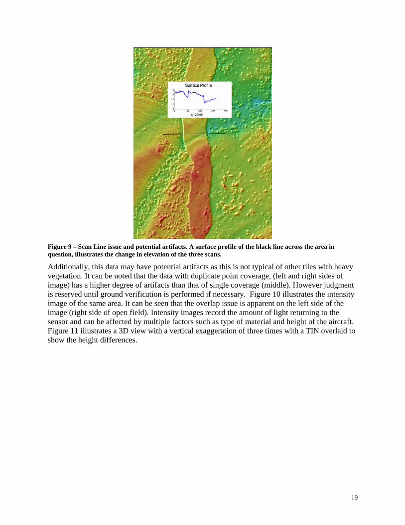
Figure 9 – Scan Line issue and potential artifacts. A surface profile of the black line across the area in question, illustrates the change in elevation of the three scans. Additionally, this data may have potential artifacts as this is not typical of other tiles with heavy vegetation. It can be noted that the data with duplicate point coverage, (left and right sides of image) has a higher degree of artifacts than that of single coverage (middle). However judgment is reserved until ground verification is performed if necessary. Figure 10 illustrates the intensity image of the same area. It can be seen that the overlap issue is apparent on the left side of the image (right side of open field). Intensity images record the amount of light returning to the sensor and can be affected by multiple factors such as type of material and height of the aircraft. Figure 11 illustrates a 3D view with a vertical exaggeration of three times with a TIN overlaid to show the height differences.

20

Figure 10 – AJ123B51: Intensity image. Note slightly different intensity values on the left side of image illustrating the change in elevation.

Figure 11 – AJ123B51: 3D view with TIN overlaid.

These height differences can happen for a multitude of reasons but the most common one is an error in the aircraft positioning. If the values are relatively small, at the one sigma level, the vegetation removal process can remove most of the error. However when they are large, then the data must be reprocessed.

21

Additional Issues Inconsistent Bridge Editing During the process of vegetation removal, artifacts consisting of both man-made and non man-made features are removed to represent a bare-earth model. With bridges, this becomes extremely difficult as parts of the structures themselves are legitimate topographic features. For example, the bridge abutments usually have earth surrounding it. This affects the flow of water and therefore elevations are required around it. As previously noted different applications may or may not require the bridge deck elevations. For this dataset, bridges can be completely removed, completely existing, or partially removed. Our preference would be to have them consistent throughout the dataset, either all in or all out. When bridge deck elevations are removed, they still exist within the vegetation file which consists of all points not representing the bare-earth terrain. By having the data consistent, no questions are directed to the integrity of the data removal in other areas such as the removal of buildings. We do not believe this constitutes reprocessing of the data. Figure 12 illustrates inconsistent bridge removal. From a hydrological point of view, removing the bridge structure over the stream is the correct process however the bridge structure on the upper right of the figure will force the flow of water in the adjacent direction of its true flow direction on a minor scale.

Figure 12 – AT116B61: Inconsistent bridge removal

Aggressive Editing Some tiles exhibited a higher degree of editing for the vegetation removal process. To understand why this was occurring, a slope map was created and the LIDAR points were

22

overlaid onto this layer. Figure 13 illustrates the correlation between high degrees of slope and the lack of LIDAR points. We understand the difficulties of establishing the balance of removing vegetation and that of topographic features especially since the vegetation removal process utilizes slope as part of its criteria whether or not to remove points. To compound the difficulty, vegetation is typically found on these slopes particularly around streams. What must be noted here is that although many points were removed, there is sufficient point density to support a two foot contour map. It should also be noted that any other technology including photogrammetry would not yield as many points and, in most cases, LIDAR is superior for topographic mapping.

Figure 13 – AQ123B61: LIDAR points overlaid on slope map. High degrees of slope yield less data.

Potential Artifacts Without ground truthing on some tiles, it is difficult to definitively identify artifacts. However looking at the ubiquitous dataset, certain patterns of terrain emerge dictating what appears to be the norm. Both Figure 9 and Figure 14 are contrary to what is typically in the surrounding data.

23

Figure 14 – AJ123B31: Potential artifacts with surface profile (cross section). Cross section location is represented by the black line to the left of the graph. Although these appear to be artifacts, undulations of between 2.4 and 2.9 meters may accurately represent terrain conditions. However there appears to be a correlation of excessive artifacts when a scan line issue exists.

Figure 15 illustrate potential artifacts and a scan line issue. The area of higher artifacts corresponds to the urban area as can be seen in Figure 16. One would expect the higher noise level to be greater in the forest located on the right side of the image.

Figure 15 – AK123B61: Potential artifacts and scan line issue.

24

Figure 16 – AK123B61: Intensity image of urban area with forested area on right side.

Conclusion Dewberry’s analysis of the data concludes that it meets the equivalency of two foot contours and is of high quality for cleanliness except for the issues listed above. We feel it important that a better quality control process be implanted by the LIDAR vendor regarding the scan line issues as this has not been seen by this vendor on past Maryland projects but is becoming more prevalent on this year’s data collection by other vendors as well. Overall it will be an excellent product to generate topographic data not only for the general user but for higher level of applications as well. As the independent QA/QC team member, the role of being independent and part of a team may appear to be a juxtaposition of terms. However, Dewberry was truly independent without any collaboration from the LIDAR vendor or post process vendors.

Appendices A and B • Follow in document titled “DNR_MD3-Howard_Anne Arundel Appendices A&B”