how would china's exports be affected by a unilateral
TRANSCRIPT

DPRIETI Discussion Paper Series 07-E-012
How Would China's Exports be Affected by a Unilateral Appreciation of the RMB and a Joint Appreciation of
Countries Supplying Intermediate Imports?
Mizanur RAHMANRIETI
Willem THORBECKERIETI
The Research Institute of Economy, Trade and Industryhttp://www.rieti.go.jp/en/

RIETI Discussion Paper Series 07-E-012
How Would China’s Exports be Affected by a
Unilateral Appreciation of the RMB and by a Joint Appreciation of Countries Supplying Intermediate
Imports?
Mizanur Rahman* National Graduate Institute for Policy Studies and RIETI
Willem Thorbecke**
George Mason University and RIETI
March 2007 Abstract: In 2005 55% of China’s exports were “processed exports” produced using intermediate goods that came from other countries. The lion’s share of the volume of imports for processing and of the value-added of processed exports came from other East Asian countries. We investigate how a unilateral appreciation of the RMB and a joint appreciation of countries supplying intermediate inputs would affect China’s exports. To do this we estimate a panel data model including ordinary and processed exports from China to 33 countries. Results obtained using generalized method of moments techniques indicate that a joint appreciation would significantly reduce China’s processed exports while a unilateral appreciation would not.
Keywords: Global imbalances; exchange rate elasticities; China
JEL classification: F32, F41 Acknowledgements: We thank Menzie Chinn, Yujiro Hayami, Kaliappa Kalirajan, Akira Kawamoto, Hisaki Kono, Kozo Oikawa, Keijiro Otsuka, Yasuyuki Sawada, Ichiro Takahara, Ryuhei Wakasugi, Masaru Yoshitomi, and seminar participants at GRIPS-FASID and RIETI for extremely valuable comments. * National Graduate Institute for Policy Studies, 7-22-1 Roppongi, Minato-ku, Tokyo 106-8677 Japan; Tel: 81-049-284-7577 ; Fax: 81-3-6439-6010; E-mail: [email protected]. ** Corresponding Author: Department of Economics, MSN 3G4, George Mason University, Fairfax, VA 22030, U.S.; Tel.: (703) 993-1151; Fax: (703) 993-1133; E-mail: [email protected] .
1
I. Introduction
China’s export growth and penetration has been remarkable. While China was
basically a closed economy 30 years ago, it is now the leading exporter to Japan, the
second leading exporter to Europe, and the third leading exporter to the U.S.
China’s explosion in exports has been accompanied by recrimination from trading
partners, especially the U.S. The U.S. Congress has blamed the enormous bilateral
deficit between the U.S. and China on the value of the RMB and has proposed retaliatory
action if China does not allow the RMB to appreciate against the dollar. Other countries
have also pushed, though less confrontationally, for an appreciation of the RMB.
Several studies investigate how an appreciation of the yuan would affect China’s
trade. Mann and Plück (2005), using a dynamic panel specification and disaggregated
trade flows, report that price elasticities for U.S. imports from China are wrong-signed
and that price elasticities for U.S. exports to China are not statistically significant.
Thorbecke (2006), employing Johansen MLE and dynamic OLS techniques, finds that
the long run real exchange rate coefficients for exports and imports between China and
the U.S. equal approximately unity. Cheung, Chinn, and Fujii (2006), using dynamic
OLS methods, find that an appreciation of the RMB increases U.S. exports to China but
does not affect China’s exports to the U.S. Marquez and Schindler (2006), using an
autoregressive distributed lag model and China’s shares in world trade, report that a 10
percent appreciation of the RMB would reduce China’s share of world exports by half a
percentage point and China’s share of world imports by a tenth of a percentage point.
Marquez and Schindler (2006) find that disaggregating Chinese trade into
processing trade and ordinary trade produces better estimates. In 2005 55% of China’s
2
exports were classified by Chinese customs authorities as “processed exports.” Processed
exports are produced using intermediate goods that are imported duty free on the
condition that the processed final goods do not enter China’s domestic market. The
lion’s share of the volume of imports for processing and of the value-added of processed
exports comes from other East Asian countries (see Gaulier et al., 2005).
Since so much of the value-added comes from other countries, it is not clear that a
unilateral appreciation of the RMB would affect the flow of processed exports much.1 A
joint appreciation of East Asian currencies would have a much larger effect on the cost of
China’s processed exports measured in the importing country’s currency. In addition, a
unilateral RMB appreciation would primarily affect the wage component of the costs of
processed exports. Since China has an excess supply of labor, wages may fall to offset
higher costs arising from a stronger exchange rate. Thus an appreciation of the RMB
alone may not reduce China’s processed exports very much.
This paper investigates how a unilateral appreciation of the RMB and a joint
appreciation among countries supplying intermediate inputs would affect China’s exports.
To do this it employs a multivariate panel data set to estimate exchange rate and income
elasticities for processed and ordinary exports from China to 33 countries. The results
indicate that an appreciation among the countries supplying imports for processing would
have a large effect on China’s exports but that a unilateral appreciation of the RMB
would not. These results imply that an appreciation of the RMB would only reduce
China’s multilateral trade surplus to the extent that it contributed to a generalized
appreciation in Asia.
1 Greenspan (2005) also makes this point.
3
The next section presents our data and methodology. Section 3 contains the
results. Section 4 concludes.
2. Data and Methodology
A. Triangular Trading Patterns
China plays a key role in global production and distribution relationships.
Multinational corporations, primarily in Japan, Korea, Taiwan and ASEAN, produce
sophisticated technology-intensive intermediate and capital goods and ship them to
China for assembly by relatively low-skilled workers. The finished products are then
exported throughout the world.
Table 1 shows China’s role in this triangular trading structure. The data are
taken from China’s Customs Statistics, which distinguishes between imports and
exports linked to processing trade and ordinary imports and exports.2 As discussed
above, imports for processing are goods that are brought into China for processing
and subsequent re-export. Processed exports, as classified by the Chinese customs
authorities, are goods that are produced in this way. Imports for processing include
both intermediate goods and capital goods.3 They are imported duty free and neither
these imported inputs nor the finished goods produced using these imports normally
enter China’s domestic market. By contrast, ordinary imports are goods that are
2 The website for China’s Customs Statistics is www.ChinaCustomsStat.com. 3 In 2003 42% of imports for processing were parts and components, 36% were semi-finished goods, 13% were capital goods, 5% were consumption goods, and 3% were primary goods. We are indebted to Deniz Unal-Kesenci for this information.

4
intended for the domestic market and ordinary exports are goods that are produced
primarily using local inputs.
Table 1 shows that in 2005 42% of China’s imports were for processing. Of
this 42%, seven-tenths came from other East Asian countries. By contrast, less than
one-twentieth each came from the U.S. and from the EU.
Table 1 also shows that in 2005 55% of China’s exports were processed
exports. Of this 55% one quarter went to the U.S., another one quarter went to East
Asia (excluding Hong Kong), one-fifth went to Hong Kong (largely as entrepôt trade),
and one fifth went to Europe.
B. Data
According to this triangular trading structure, most of the value-added for Chinese
processed exports comes from other (primarily East Asian) countries. Thus a unilateral
appreciation of the RMB would not affect the costs of Chinese processed exports
measured in the importing country’s currency as much as a generalized appreciation of
East Asian currencies. It is possible to differentiate between the effects of a unilateral
RMB appreciation and a multilateral appreciation by employing trade-weighted exchange
rates. Suppose one is trying to explain Chinese processed exports to another country (e.g.,
Australia). Suppose also that China’s imports for processing come 35% from Japan, 35%
from Taiwan, and 30% from Korea. Then to explain Chinese exports to Australia one of
the explanatory variables, along with the Australian $/RMB bilateral exchange rate,
would be the weighted exchange rate ( Auswrer ) between the countries supplying imports

5
for processing and Australia (i.e., 0.35*Australian $/Yen + 0.35* Australian $/NT $ +
0.30 Australian $/Won) .
To calculate weighted exchange rates in this way we need to measure the bilateral
exchange rates using a common numeraire. We can do this by employing the real
exchange rate variables constructed by the Centre D’Etudes Prospectives et
D’Information Internationales (CEPII). These variables compare observed exchange
rates to PPP ones, and exceed 100 when the currency is overvalued. They are thus
comparable both cross sectionally and over time. These variables are obtained from the
CEPII-CHELEM database.
When calculating weights we include every country that supplies at least one
percent of the total value of imports for processing to China. We determine weights for
these countries by dividing their contribution to China’s processed imports by the amount
of processed imports coming from all countries supplying at least one percent of the total.
As discussed above, we can then use these weights to find the weighted exchange rate
( iwrer ) for a country i that purchases China’s processed exports by calculating the inner
product of the weights and the bilateral real exchange rates between the countries
supplying imports for processing and country i. We recalculate the weights and iwrer
each year.
We include in our estimation iwrer and the bilateral RMB real exchange rate
( irer ) with the importing country i. We also include real income in the importing country
( irgdp ), the Chinese capital stock in manufacturing ( iK ), and a set of gravity variables.
irgdp is measured in millions of PPP dollars. iK is measured at constant prices. The
gravity variables include distance and dummy variables indicating whether the two

6
countries are contiguous, share a common language, and have a colonial link. The real
GDP data come from the CEPII-CHELEM database, the Chinese capital stock data are
constructed by Bai, Hsieh, and Qian (2006), and the gravity variables are obtained from
www.cepii.fr.
Our panel is composed of processed and ordinary exports from China to 33
countries over the 1992-2005 period.4 The advantage of this data set is that, while the
U.S. dollar/RMB exchange rate has not changed very much, there has been substantial
variation both cross-sectionally and over time in irer w and irer relative to the 33
countries purchasing exports. This approach should thus help us to identify in an
econometric sense how exchange rate changes affect China’s multilateral exports.5
Data on imports for processing and on ordinary and processed exports are
obtained from China’s Customs Statistics. The data are all measured in U.S. dollars.
We deflate the export data in three ways. First, following Cheung, Chinn, and
Fujii (2006), we deflate Chinese exports using the U.S. Bureau of Labor Statistics (BLS)
price deflator for imports from non-industrial countries. Cheung et al. find that this series
closely matches the BLS price deflator for imports from China, which became available
in 2003. Second, we use the Hong Kong export price deflator. Since many of Hong
Kong’s exports are re-exports from China, this measure may be a useful proxy for
Chinese export prices. Third, following Eichengreen et al. (2004), we use the U.S.
4 The countries are: Argentina, Australia, Austria, Belgium, Brazil, Canada, Denmark, Finland, France, Germany, Greece, Hong Kong, Indonesia, Iceland, Ireland, Italy, Japan, Luxembourg, Malaysia, Mexico, the Netherlands, New Zealand, the Philippines, Portugal, Russian Federation, Singapore, South Korea, Spain, Sweden, Taiwan, Thailand, the United Kingdom, and the United States. 5 It is particularly difficult to investigate the effects of a change in the bilateral RMB exchange rate holding the weighted exchange rate constant. However, since currencies such as the yen and won have fluctuated substantially against the dollar while the RMB has not, there may be enough independent variation in
irer w and irer across the 33 countries to make it possible to estimate the individual parameters.
7
consumer price index to deflate China’s exports. This measure would be appropriate if
the bundle of goods and services exported from China corresponds to the bundle
purchased by U.S. consumers. The results reported below are very similar regardless of
which deflator we use.
C. The Imperfect Substitutes Framework
According to the imperfect substitutes model of Goldstein and Khan (1985), the
quantity of China’s exports demanded by other countries depends on income in the other
countries and the price of China’s exports relative to the price of domestically produced
goods in those countries. The quantity of exports supplied by China depends on the
export price relative to China’s price level. By equating demand and supply one can
derive an export function (see, e.g., Chinn, 2005):
tex = α10 + α11 trer + α12t *trgdp + ε1t (2)
where tex represents real exports, trer represents the real exchange rate, and *rgdp
represents foreign real income.
If the elasticity of supply is infinite, it is possible to identify the parameters in
equation (1). In the case of China’s exports there are reasons to believe that the perfect
supply elasticity assumption is reasonable. China has between 150 and 200 million
redundant rural laborers, 7-8 million new workers joining the labor force each year, and
8
14 million urban workers who are unemployed or underemployed.6 This large pool of
workers seeking employment in the export sector may enable Chinese exporters to
increase supply at constant prices.
In addition, as the IMF (2005) argues, the supply of imports for processing will
vary one for one with the demand for processed exports. Marquez and Schindler (2006)
present formal evidence supporting this assertion. They report that the coefficient on
imports for processing is nearly always one in regressions where the dependent variable
is China’s processed exports. Thus sophisticated intermediate and capital goods tend to
flow elastically into China’s processed export industries to accommodate increases in
demand in the rest of the world.
We do attempt to control for any changes in the supply of exports by including
the Chinese capital stock in manufacturing. Cheung, Chinn, and Fujii (2006) employ this
variable as a proxy for China’s supply capacity.7
D. The Econometric Model
To determine the appropriate econometric specification we first investigate the
time series properties of the data. As reported in the Appendix, Levin-Lin-Chu panel unit
root tests indicate that real exports and real gross domestic product are trend stationary
series following first-order autoregressive error processes. The tests also indicate that the
exchange rate variables are I(0) stationary series.
Since our model contains lagged values of the dependent variable, the error term
will be correlated with a right hand side variable. Arellano and Bond (1991) propose a
6 We are indebted to the Chinese Academy of Social Sciences for these data. 7 The series on China’s capital stock in manufacturing was constructed by Bai, Hsieh, and Qian (2006).
9
generalized method of moments (GMM) estimator to correct for the resulting bias. They
recommend first-differencing the equation to be estimated and then using lagged values
of the levels as instruments.
Blundell and Bond (1998) show that if the variables employed as instruments are
persistent over time, lagged levels of these variables will be weak instruments and the
resulting coefficient estimates will be biased in small samples. Results presented in the
Appendix indicate that the variables are persistent.
We thus use the extended instrument matrix proposed by Blundell and Bond
(1998) and employ GMM system estimation rather than GMM first-difference techniques.
To avoid overfitting, we collapse the instrument matrix. The instruments we employ are
presented in the Appendix.
To model the individual export equations we use an autoregressive distributed lag
model of order 2,2:
)3(.,,1;,,3
,
2211
0221102211
02211022110
NiTt
uzKKKrgdprgdprgdpwrerwrer
wrerrerrerrerexexex
ititt
tititititit
ititititititit
LL ==
++′+++++++++
++++++=
−−
−−−−
−−−−
μψαααλλληη
ηγγγβββ
Here itex represents real exports (either processed or ordinary) from China to country i ,
itrer represents the bilateral real exchange rate between China and country i (an
increase denotes an appreciation of the Chinese real exchange rate), itwrer represents the
multilateral weighted real exchange rate between countries providing imports for
processing to China and country i that purchases exports from China (an increase
10
represents an appreciation of the weighted exchange rate), itrgdp equals real income in
the importing country, tK denotes the Chinese capital stock in manufacturing, z is a set
of gravity variables (distance and dummy variables indicating whether the two countries
are contiguous, share a common language, and have a colonial link), and iμ is a country
i fixed effect. The variables are measured in natural logs. itex , itrer , itwrer , and itrgdp
vary both over time and across countries; z only varies across countries.; and tK only
varies across time. Our sample includes annual exports to 33 countries over the 1992-
2005 period.
3. Results
Tables 2 and 3 present our basic findings. Focusing first on the diagnostic tests,
Hansen’s J-statistics for all specifications in both tables are too small to reject the null
hypothesis that the instruments are valid. The m1 and m2 test statistics for first- and
second-order serial correlation in the first-differenced residuals indicate, as required, that
while we can often reject the null hypothesis of no first-order autocorrelation we cannot
reject the null hypothesis of no second-order autocorrelation at the 5 percent level.
Table 2 presents results for processed exports. Exports are deflated using all three
deflators. In all three cases, the model is estimated once including gravity variables and a
trend term and once excluding these. The results are similar across all six specifications.
The income coefficient is positive and statistically significant in every
specification. The income elasticity is about 3. The relatively high income elasticity
probably reflects the fact that many of the processed exports are sophisticated, high-tech
goods that consumers are more likely to purchase as their incomes increase.

11
The coefficient on the weighted exchange rate is of the expected negative sign,
indicating that an appreciation of wrer reduces processed exports. The coefficient is
statistically significant in every specification and the elasticity averages about 2. The
coefficient on the RMB exchange rate, however, is of the wrong sign in every
specification. These results indicate that it is the exchange rates among countries
supplying intermediate imports rather than the RMB exchange rate that matters for
China’s processed exports.
Finally, the Chinese capital stock variable is always positive and significant. The
coefficients range from 3 to 4.75. Cheung, Chinn, and Fujii (2006) also reported
positive and significant values for this variable, with coefficients ranging from 1.5 to 4.5.
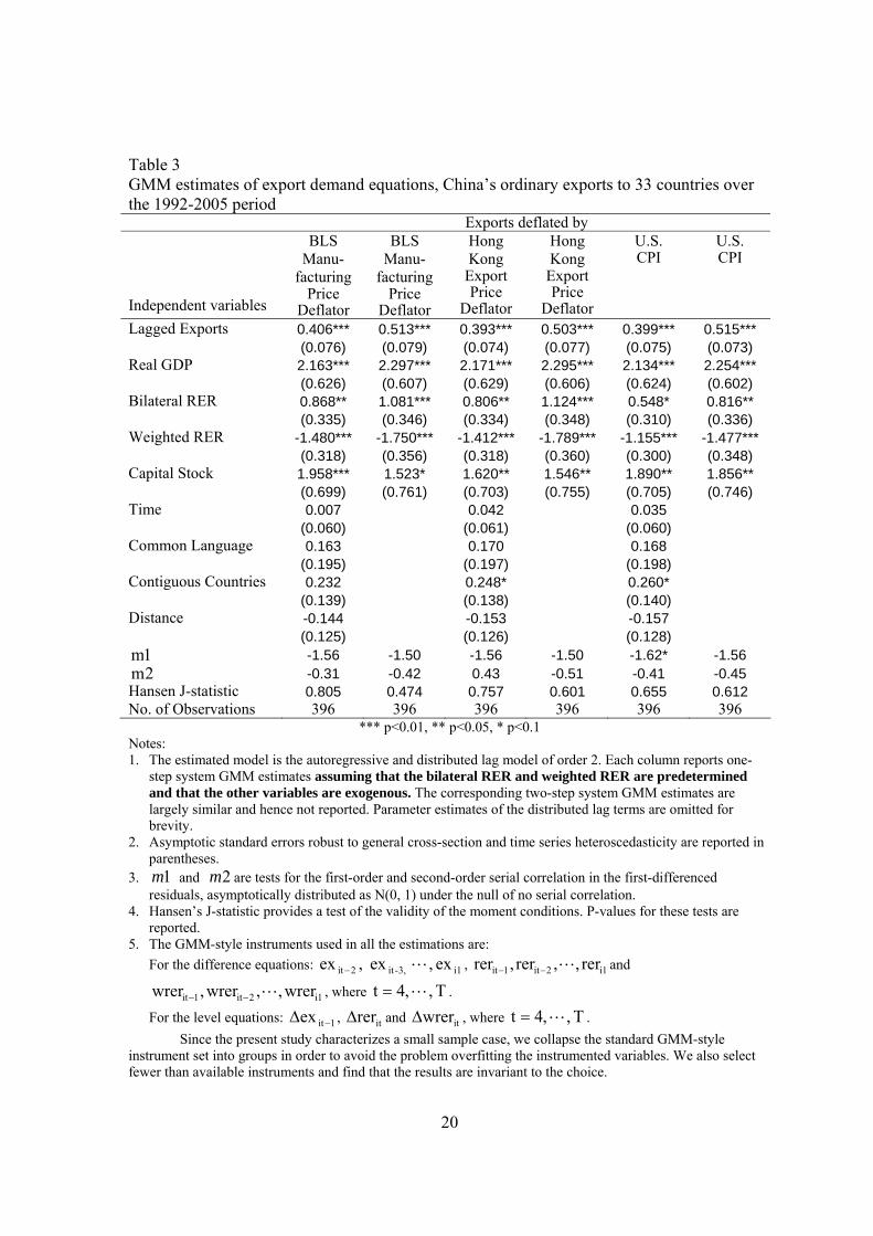
Table 3 presents our findings for ordinary exports. Exports are again deflated
using all three deflators and the model is again estimated both including gravity variables
and a trend term and excluding these. The results are similar across the six specifications.
The income coefficient is positive and statistically significant in every case. The
income elasticity averages a little more than 2. These values are less than the elasticities
for processed exports. This probably reflects the fact that, compared with processed
exports, ordinary exports contain more traditional goods and lower-value added products
(e.g., toys) that have lower income elasticities of demand.
The coefficient on the weighted exchange rate is of the expected negative sign,
indicating that an appreciation of wrer reduces ordinary exports. The coefficient is
statistically significant in every specification and the elasticity averages about 1.5. The
coefficient on the RMB exchange rate, however, is of the wrong sign in every case.
These results indicate that it is the exchange rate among countries supplying intermediate

12
imports rather than the RMB exchange rate that matters for China’s ordinary exports.
Finally, the Chinese capital stock variable is always positive and statistically
significant. The coefficients range from 1.5 to 2. These values are smaller than those
reported in Table 2 for processed exports. This perhaps reflects the fact that ordinary
exports are produced using less capital-intensive technologies.
Tables 4-7 test the robustness of the findings reported in Tables 2 and 3. They
include specifications without the capital stock and specifications where rer and
wrer are treated as exogenous rather than predetermined. Across all the specifications,
the elasticities for income and wrer remain of the expected signs and statistically
significant and the elasticity for rer remains either of the wrong sign or of the right sign
but not statistically significant. Thus the evidence in Tables 4-7 supports the results
presented in Tables 2 and 3.
An important implication of these findings is that what matters for China’s
exports is not the RMB exchange rate but the weighted exchange rate among countries
supplying intermediate imports. According to these results, an RMB appreciation would
reduce China’s exports only to the extent that it contributed to a generalized appreciation
in Asia.
A second important implication of these results is that a slowdown in the rest of
the world would significantly reduce processing trade. The income elasticity for
processed exports equals 3. A downturn outside of Asia could thus cause a large drop in
China’s processed exports. This in turn would decrease the flow of intermediate goods
from the rest of Asia into China, reducing employment and output throughout the region.
4. Conclusion

13
China has progressed from being virtually a closed economy 30 years ago to
being the largest exporter of manufactured goods in 2006. This surge in exports has been
accompanied by recrimination from trading partners, especially the U.S. The U.S.
Congress has demanded that China let the RMB appreciate.
Greenspan (2005) and others have argued that, because of triangular trading
patterns in Asia, a unilateral appreciation of the RMB would not affect China’s exports
much. We investigate how a unilateral appreciation of the RMB and a joint appreciation
among countries supplying intermediate inputs would affect China’s exports. To do this
we estimate a panel that includes ordinary and processed exports from China to 33
countries. The results indicate that a joint appreciation would significantly reduce
China’s multilateral exports but that a unilateral appreciation would not.
A move towards a more flexible regime in China might nonetheless help to
resolve global trade imbalances. There is currently a prisoner’s dilemma problem in East
Asia. Fear of losing competitiveness relative to other Asian economies causes individual
countries in the region to prevent their currencies from appreciating (see Ogawa and Ito,
2002).
This problem could be mitigated if China and other countries in the region with
less flexible exchange rates adopted more flexible regimes. In this case the large
surpluses that East Asia is running in processing trade would allow currencies in the
region to appreciate together. If market forces led to joint appreciations in this way, they
would help to maintain relatively stable intra-regional exchange rates in the face of the
current global imbalances.8
8 Relatively stable exchange rates within East Asia would provide other benefits. They would attenuate effective exchange rate changes arising from currency appreciations since intra-regional
14
For China and other developing Asian countries more flexible regimes could be
characterized by 1) multiple currency basket-based reference rates instead of a dollar-
based central rate, and 2) wider bands around the reference rate. Greater exchange rate
flexibility in the context of a multiple currency basket-based reference rate would
probably be preferable to a free floating regime for Asian countries with underdeveloped
financial institutions. It would allow their currencies to appreciate in response to global
imbalances but still enable policy makers to limit excessive volatility.
China’s global current account surplus in 2006 exceeded 8 percent of Chinese
GDP. The Chinese government, in its 2006-2010 five year plan, recognized the need to
rebalance its economy. The results reported here indicate that an RMB appreciation
alone would not help to achieve this goal. However, if an RMB appreciation led to a
generalized appreciation in the region, it would be effective. A generalized appreciation
would also help to maintain relative exchange rate stability in Asia. This, in turn, would
provide a steady backdrop for the regional production and distribution networks that have
led to enormous efficiency gains in recent years.
References
Anderson, T. W., and Hsiao, C. 1981. Estimation of Dynamic Models with Error Components. Journal of the American Statistical Association, 76(375): 598-606.
trade accounts for 55% of total trade. They would also help to maintain FDI flows and provide a steady backdrop for regional production and distribution networks. See Yoshitomi et al. (2005) for a discussion of these issues.
15
Anderson, T. W., and Hsiao, C. 1982. Formulation and Estimation of Dynamic Models Using Panel Data. Journal of Econometrics 18, 47-82.
Arellano, M., and Bond, S.R. 1991. Some Tests of Specification for Panel Data: Monte Carlo Evidence and an Application to Employment Equations. Review of Economic Studies, 58, 277-297. Arellano, M., and Bover, O. 1995. Another Look at the Instrumental-variable Estimation
of Error-components Models. Journal of Econometrics, 68: 29-51. Bai, C., Hsieh,C., and Qian, Q. 2006. Returns to Capital in China. Brookings Papers on
Economic Activity forthcoming. Blundell, R.W., and Bond, S.R. 1998. Initial Conditions and Moment Restrictions in
Dynamic Panel Data Models. Journal of Econometrics 87, 115-143. Breitung, J., and Pesaran, H. forthcoming. Unit Roots and Cointegration in Panels. In L. Matyas and P. Sevestre, (eds.), The Econometrics of Panel Data:
Fundamentals and Recent Developments in Theory and Practice, Kluwer, Boston.
Cheung, Y., Chinn, M., and Fujii, E. 2006. China’s Current Account and Exchange Rate. Paper presented at NBER Conference on China’s Growing Role in World
Trade, Cambridge, MA, 14 October 2006. Chinn, M. 2005. Doomed to Deficits? Aggregate U.S. Trade Flows Re-visited. Review of World Economics 141, 460-85. Eichengreen, B., Rhee, Y., and Tong, H. 2004. The Impact of China on the Exports of Other Asian Countries, NBER Working Paper No. 10768, National Bureau of Economic Research, Cambridge, MA. Fuller, W.A. 1976. Introduction to Statistical Time Series. John Wiley & Sons, Inc., New York. Gaulier, G., Lemoine, F., and Unal-Kesenci, D. 2005. China’s Integration in East Asia:
Production Sharing, FDI, and High-tech Trade. CEPII Working Paper No. 2005-09, Centre D’Etudes Prospectives et D’Information Internationales, Paris.
Greenspan, A. 2005. China. Testimony before the U.S. Senate Committee on Finance, 23 June 2005, Federal Reserve Board, Washington, DC. Hansen, L. P., 1982. Large Sample Properties of Generalized Method of Moments Estimators. Econometrica 50, 1029-1054.
16
Holtz-Eakin, Newey, D., W. and Rosen, H. 1988. Estimating Vector Autoregressions with Panel Data. Econometrica, 56: 1371-1395.
IMF, 2005. Asia-Pacific Economic Outlook, International Monetary Fund, Washington, DC. Levin, A., Lin, C., and Chu, C. 2002. Unit Roots in Panel Data: Asymptotic and Finite- Sample Properties. Journal of Econometrics 108, 1-24. Mann, C. L., and Plück, K. 2005. The US Trade Deficit: A Disaggregated Perspective.IIE Working Paper No. WP 05-11. Institute for International Economics, Washington, DC. Marquez, J. and Schindler, J. 2006. Exchange Rate Effects on China’s Trade: An Interim Report. International Finance Discussion Paper, No. 861. Federal Reserve Board, Washington, DC. Nickell, S. 1981. Biases in Dynamic Models with Fixed Effects. Econometrica, 49: 1417-
1426. Ogawa, E., and Ito, T. 2002. On the Desirability of a Regional Basket Currency Arrangement. Journal of the Japanese and International Economies 16, 317-334. Pesaran, M. H. 2003. A Simple Panel Unit Root Test in the Presence of Cross Section
Dependence. Cambridge Working Papers in Economics 0346, Faculty of Economics (formerly DAE), University of Cambridge.
Sims, C., Stock, J., and Watson, M. 1990. Inference in Linear Time Series Models with
Some Unit Roots. Econometrica 58, 113-144. Thorbecke, W. 2006. How Would an Appreciation of the Renminbi Affect the U.S.
Trade Deficit with China? The B.E. Journal in Macroeconomics 6, No. 3, Article 3.
Yoshitomi, M., Liu, L., and Thorbecke, W. 2005. East Asia’s Role in Resolving the New Global Imbalances. Research Institute of Economy, Trade and Industry (RIETI), Tokyo.
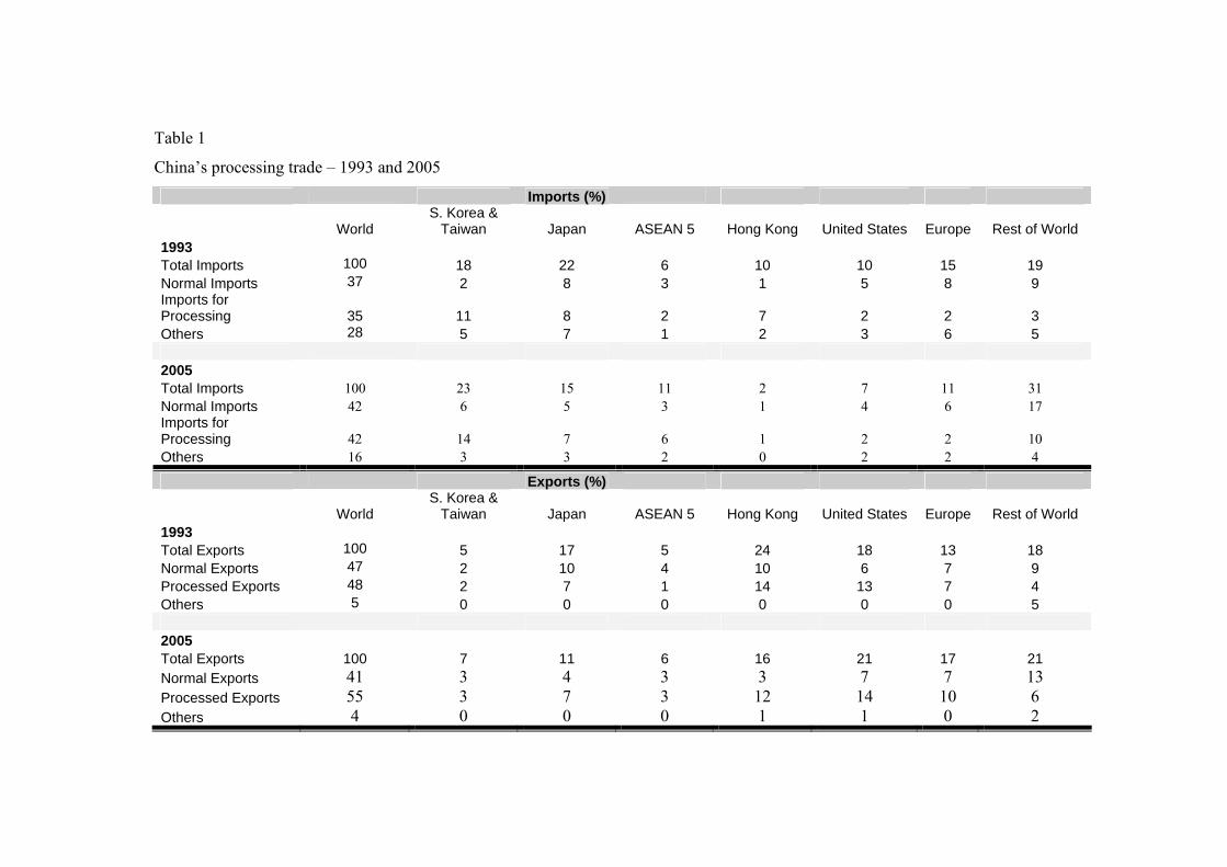
Table 1
China’s processing trade – 1993 and 2005
Imports (%)
World S. Korea &
Taiwan Japan ASEAN 5 Hong Kong United States Europe Rest of World 1993 Total Imports 100 18 22 6 10 10 15 19 Normal Imports 37 2 8 3 1 5 8 9 Imports for Processing
35 11 8 2 7 2 2 3
Others 28 5 7 1 2 3 6 5 2005 Total Imports 100 23 15 11 2 7 11 31 Normal Imports 42 6 5 3 1 4 6 17 Imports for Processing 42 14 7 6 1 2 2 10 Others 16 3 3 2 0 2 2 4
Exports (%)
World S. Korea &
Taiwan Japan ASEAN 5 Hong Kong United States Europe Rest of World 1993 Total Exports 100 5 17 5 24 18 13 18 Normal Exports 47 2 10 4 10 6 7 9 Processed Exports 48 2 7 1 14 13 7 4 Others 5 0 0 0 0 0 0 5 2005 Total Exports 100 7 11 6 16 21 17 21 Normal Exports 41 3 4 3 3 7 7 13 Processed Exports 55 3 7 3 12 14 10 6 Others 4 0 0 0 1 1 0 2

18
Table 1 (continued).
China’s processing trade – 1993 and 2005
Balance of Trade (billions of US Dollars)
1993
World S. Korea &Taiwan Japan ASEAN 5 Hong Kong United States Europe Rest of World
Balance of trade -12.2 -14.0 -7.5 -1.3 11.60 6.3 -3.5 -3.8 Normal trade 5.2 0.3 0.7 -0.1 7.7 0 -2 -1.5 Processing trade 7.9 -9.5 -1.3 -0.6 5.7 9.7 4.2 -0.3 Others -25.2 -4.9 -6.9 -0.6 -1.7 -3.4 -5.8 -1.9 2005 Balance of trade 102.00 -99.84 -16.42 -23.81 112.25 114.27 61.37 -45.81 Normal trade 35.43 -12.91 -2.45 1.95 21.59 26.91 14.36 -14.01 Processing trade 142.46 -69.25 4.49 -13.31 85.05 92.94 60.42 -17.88 Others -75.88 -17.69 -18.46 -12.44 5.61 -5.58 -13.41 -13.91
Notes: Source: Gaulier, Lemoine, and Nal-Kesenci (2005), China’s Customs Statistics, and calculations by the authors. Europe includes Austria, Belgium, Denmark, Finland, France, Germany, Greece, Luxembourg, Netherlands, Italy, Portugal, Spain, and Sweden.

19
Table 2 GMM estimates of export demand equations, China’s processed exports to 33 countries over the 1992-2005 period Exports deflated by Independent variables
BLS Manu-
facturing Price
Deflator
BLS Manu-
facturingPrice
Deflator
Hong Kong
Export Price
Deflator
Hong Kong Export Price
Deflator
U.S. CPI
U.S. CPI
Lagged Exports 0.675*** 0.696*** 0.659*** 0.678*** 0.663*** 0.677*** (0.072) (0.067) (0.072) (0.066) (0.072) (0.065) Real GDP 2.809*** 3.021*** 2.826*** 3.038*** 2.817*** 3.038*** (0.475) (0.583) (0.480) (0.586) (0.486) (0.597) Bilateral RER 1.990*** 1.543*** 1.884*** 1.536*** 1.678*** 1.290** (0.525) (0.473) (0.523) (0.476) (0.514) (0.480) Weighted RER -2.534*** -1.970*** -2.422*** -1.954*** -2.214*** -1.699*** (0.531) (0.392) (0.524) (0.391) (0.512) (0.391) Capital Stock 4.754** 3.076** 4.337** 3.058** 4.658** 3.319** (1.909) (1.348) (1.884) (1.352) (1.906) (1.375) Time -0.168 -0.134 -0.143 (0.117) (0.117) (0.115) Common Language 0.174 0.180 0.178 (0.188) (0.189) (0.190) Contiguous Countries 0.100 0.110 0.118 (0.130) (0.130) (0.129) Distance -0.119 -0.126 -0.129 (0.099) (0.100) (0.101)
1m -2.88*** -2.99*** -2.85*** -2.94*** -2.80*** -2.89***2m -0.91 -1.29 -1.00 -1.37 -1.01 -1.35
Hansen J-statistic 0.882 0.604 0.842 0.683 0.877 0.708 No. of Observations 396 396 396 396 396 396
*** p<0.01, ** p<0.05, * p<0.1 Notes: 1. The estimated model is the autoregressive and distributed lag model of order 2. Each column reports one-
step system GMM estimates assuming that the bilateral RER and weighted RER are predetermined and that the other variables are exogenous. The corresponding two-step system GMM estimates are largely similar and hence not reported. Parameter estimates of the distributed lag terms are omitted for brevity.
2. Asymptotic standard errors robust to general cross-section and time series heteroscedasticity are reported in parentheses.
3. 1m and 2m are tests for the first-order and second-order serial correlation in the first-differenced residuals, asymptotically distributed as N(0, 1) under the null of no serial correlation.
4. Hansen’s J-statistic provides a test of the validity of the moment conditions. P-values for these tests are reported.
5. The GMM-style instruments used in all the estimations are: For the difference equations: i13,-it2it ex, ex ,ex L− , 1i2it1it rer,,rer,rer L−− and
1i2it1it wrer,,wrer,wrer L−− , where T,,4t L= .
For the level equations: 1itex −Δ , itrerΔ and itwrerΔ , where T,,4t L= . Since the present study characterizes a small sample case, we collapse the standard GMM-style instrument set into groups in order to avoid the problem overfitting the instrumented variables. We also select fewer than available instruments and find that the results are invariant to the choice.
20
Table 3 GMM estimates of export demand equations, China’s ordinary exports to 33 countries over the 1992-2005 period Exports deflated by Independent variables
BLS Manu-
facturing Price
Deflator
BLS Manu-
facturingPrice
Deflator
Hong Kong
Export Price
Deflator
Hong Kong Export Price
Deflator
U.S. CPI
U.S. CPI
Lagged Exports 0.406*** 0.513*** 0.393*** 0.503*** 0.399*** 0.515*** (0.076) (0.079) (0.074) (0.077) (0.075) (0.073) Real GDP 2.163*** 2.297*** 2.171*** 2.295*** 2.134*** 2.254*** (0.626) (0.607) (0.629) (0.606) (0.624) (0.602) Bilateral RER 0.868** 1.081*** 0.806** 1.124*** 0.548* 0.816** (0.335) (0.346) (0.334) (0.348) (0.310) (0.336) Weighted RER -1.480*** -1.750*** -1.412*** -1.789*** -1.155*** -1.477*** (0.318) (0.356) (0.318) (0.360) (0.300) (0.348) Capital Stock 1.958*** 1.523* 1.620** 1.546** 1.890** 1.856** (0.699) (0.761) (0.703) (0.755) (0.705) (0.746) Time 0.007 0.042 0.035 (0.060) (0.061) (0.060) Common Language 0.163 0.170 0.168 (0.195) (0.197) (0.198) Contiguous Countries 0.232 0.248* 0.260* (0.139) (0.138) (0.140) Distance -0.144 -0.153 -0.157 (0.125) (0.126) (0.128)
1m -1.56 -1.50 -1.56 -1.50 -1.62* -1.56 2m -0.31 -0.42 0.43 -0.51 -0.41 -0.45
Hansen J-statistic 0.805 0.474 0.757 0.601 0.655 0.612 No. of Observations 396 396 396 396 396 396
*** p<0.01, ** p<0.05, * p<0.1 Notes: 1. The estimated model is the autoregressive and distributed lag model of order 2. Each column reports one-
step system GMM estimates assuming that the bilateral RER and weighted RER are predetermined and that the other variables are exogenous. The corresponding two-step system GMM estimates are largely similar and hence not reported. Parameter estimates of the distributed lag terms are omitted for brevity.
2. Asymptotic standard errors robust to general cross-section and time series heteroscedasticity are reported in parentheses.
3. 1m and 2m are tests for the first-order and second-order serial correlation in the first-differenced residuals, asymptotically distributed as N(0, 1) under the null of no serial correlation.
4. Hansen’s J-statistic provides a test of the validity of the moment conditions. P-values for these tests are reported.
5. The GMM-style instruments used in all the estimations are: For the difference equations: i13,-it2it ex, ex ,ex L− , 1i2it1it rer,,rer,rer L−− and
1i2it1it wrer,,wrer,wrer L−− , where T,,4t L= .
For the level equations: 1itex −Δ , itrerΔ and itwrerΔ , where T,,4t L= . Since the present study characterizes a small sample case, we collapse the standard GMM-style instrument set into groups in order to avoid the problem overfitting the instrumented variables. We also select fewer than available instruments and find that the results are invariant to the choice.

21
Table 4 GMM estimates of export demand equations, China’s processed exports to 33 countries over the 1992-2005 period Exports deflated by Independent variables
BLS Manu-
facturing Price
Deflator
BLS Manu-
facturingPrice
Deflator
Hong Kong
Export Price
Deflator
Hong Kong Export Price
Deflator
U.S. CPI
U.S. CPI
Lagged Exports 0.741*** 0.783*** 0.732*** 0.778*** 0.760*** 0.835*** (0.073) (0.065) (0.073) (0.064) (0.072) (0.061) Real GDP 2.779*** 2.691*** 2.776*** 2.714*** 2.856*** 2.778*** (0.542) (0.657) (0.541) (0.654) (0.555) (0.650) Bilateral RER 0.602* 0.061 0.565 0.114 0.344 0.130 (0.349) (0.318) (0.349) (0.317) (0.361) (0.339) Weighted RER -1.288*** -0.679** -1.251*** -0.732** -1.026*** -0.782*** (0.366) (0.274) (0.364) (0.273) (0.369) (0.281) Capital Stock Time -0.012 -0.007 0.013 (0.018) (0.018) (0.017) Common Language 0.241 0.239 0.244 (0.172) (0.175) (0.171) Contiguous Countries 0.160 0.163 0.185* (0.110) (0.111) (0.108) Distance -0.168* -0.168 -0.179* (0.098) (0.099) (0.102)
1m -2.97*** -3.08*** -2.95*** -3.06*** -2.97*** -3.09***2m -0.53 -0.87 -0.66 -0.95 -0.46 -0.71
Hansen J-statistic 0.735 0.596 0.758 0.618 0.712 0.559 No. of Observations 396 396 396 396 396 396
*** p<0.01, ** p<0.05, * p<0.1 Notes: 1. The estimated model is the autoregressive and distributed lag model of order 2. The model excludes the
capital stock variable in all cases. Each column reports one-step system GMM estimates assuming that the bilateral RER and weighted RER are predetermined and that the other variables are exogenous. The corresponding two-step system GMM estimates are largely similar and hence not reported. Parameter estimates of the distributed lag terms are omitted for brevity.
2. Asymptotic standard errors robust to general cross-section and time series heteroscedasticity are reported in parentheses.
3. 1m and 2m are tests for the first-order and second-order serial correlation in the first-differenced residuals, asymptotically distributed as N(0, 1) under the null of no serial correlation.
4. Hansen’s J-statistic provides a test of the validity of the moment conditions. P-values for these tests are reported.
5. The GMM-style instruments used in all the estimations are: For the difference equations: i13,-it2it ex, ex ,ex L− , 1i2it1it rer,,rer,rer L−− and
1i2it1it wrer,,wrer,wrer L−− , where T,,4t L= .
For the level equations: 1itex −Δ , itrerΔ and itwrerΔ , where T,,4t L= . Since the present study characterizes a small sample case, we collapse the standard GMM-style instrument set into groups in order to avoid the problem overfitting the instrumented variables. We also select fewer than available instruments and find that the results are invariant to the choice.

22
Table 5 GMM estimates of export demand equations, China’s ordinary exports to 33 countries over the 1992-2005 period Exports deflated by Independent variables
BLS Manu-
facturing Price
Deflator
BLS Manu-
facturingPrice
Deflator
Hong Kong
Export Price
Deflator
Hong Kong Export Price
Deflator
U.S. CPI
U.S. CPI
Lagged Exports 0.485*** 0.521*** 0.475*** 0.516*** 0.517*** 0.561*** (0.092) (0.081) (0.089) (0.080) (0.096) (0.081) Real GDP 1.901*** 1.897*** 1.880*** 1.899*** 1.859*** 1.895*** (0.648) (0.638) (0.651) (0.636) (0.645) (0.627) Bilateral RER 0.105 -0.323 0.102 -0.249 -0.274 -0.313 (0.292) (0.193) (0.294) (0.192) (0.266) (0.198) Weighted RER -0.888*** -0.449*** -0.887*** -0.526*** -0.531** -0.522*** (0.270) (0.149) (0.270) (0.148) (0.251) (0.157) Capital Stock Time -0.013 -0.008 0.012 (0.025) (0.024) (0.024) Common Language 0.064 0.067 0.032 (0.162) (0.158) (0.160) Contiguous Countries 0.134 0.140 0.138 (0.144) (0.139) (0.157) Distance -0.075 -0.078 -0.068 (0.112) (0.110) (0.114)
1m -1.66 -1.65 -1.67* -1.66* -1.79* -1.76* 2m 0.40 -0.60 -0.51 -0.68 -0.41 -0.55
Hansen J-statistic 0.672 0.604 0.677 0.570 0.574 0.488 No. of Observations 396 396 396 396 396 396
*** p<0.01, ** p<0.05, * p<0.1 Notes: 1. The estimated model is the autoregressive and distributed lag model of order 2. The model excludes the
capital stock variable in all cases. Each column reports one-step system GMM estimates assuming that the bilateral RER and weighted RER are predetermined and that the other variables are exogenous. The corresponding two-step system GMM estimates are largely similar and hence not reported. Parameter estimates of the distributed lag terms are omitted for brevity.
2. Asymptotic standard errors robust to general cross-section and time series heteroscedasticity are reported in parentheses.
3. 1m and 2m are tests for the first-order and second-order serial correlation in the first-differenced residuals, asymptotically distributed as N(0, 1) under the null of no serial correlation.
4. Hansen’s J-statistic provides a test of the validity of the moment conditions. P-values for these tests are reported.
5. The GMM-style instruments used in all the estimations are: For the difference equations: i13,-it2it ex, ex ,ex L− , 1i2it1it rer,,rer,rer L−− and
1i2it1it wrer,,wrer,wrer L−− , where T,,4t L= .
For the level equations: 1itex −Δ , itrerΔ and itwrerΔ , where T,,4t L= . Since the present study characterizes a small sample case, we collapse the standard GMM-style instrument set into groups in order to avoid the problem overfitting the instrumented variables. We also select fewer than available instruments and find that the results are invariant to the choice.
23
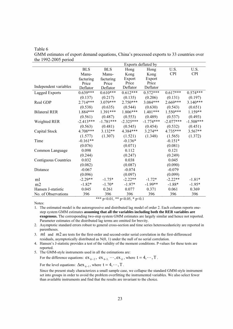
Table 6 GMM estimates of export demand equations, China’s processed exports to 33 countries over the 1992-2005 period Exports deflated by Independent variables
BLS Manu-
facturing Price
Deflator
BLS Manu-
facturingPrice
Deflator
Hong Kong
Export Price
Deflator
Hong Kong Export Price
Deflator
U.S. CPI
U.S. CPI
Lagged Exports 0.639*** 0.610*** 0.612*** 0.572*** 0.617*** 0.574*** (0.137) (0.217) (0.135) (0.206) (0.131) (0.197) Real GDP 2.714*** 3.079*** 2.750*** 3.084*** 2.669*** 3.140*** (0.538) (0.635) (0.544) (0.630) (0.543) (0.651) Bilateral RER 1.884*** 1.391*** 1.806*** 1.401*** 1.550*** 1.159** (0.561) (0.487) (0.553) (0.489) (0.537) (0.493) Weighted RER -2.413*** -1.781*** -2.325*** -1.774*** -2.077*** -1.508*** (0.563) (0.481) (0.545) (0.454) (0.532) (0.451) Capital Stock 4.708*** 3.132** 4.384*** 3.274** 4.735*** 3.567** (1.577) (1.307) (1.521) (1.348) (1.565) (1.372) Time -0.161** -0.136* -0.151* (0.076) (0.071) (0.081) Common Language 0.098 0.112 0.121 (0.244) (0.247) (0.249) Contiguous Countries 0.032 0.038 0.045 (0.082) (0.087) (0.090) Distance -0.067 -0.074 -0.079 (0.096) (0.097) (0.099)
1m -2.29** -1.75* -2.22** -1.72* -2.22** -1.81* 2m -1.82* -1.70* -1.97* -1.99** -1.88* -1.95*
Hansen J-statistic 0.045 0.261 0.077 0.371 0.061 0.369 No. of Observations 396 396 396 396 396 396
*** p<0.01, ** p<0.05, * p<0.1 Notes: 1. The estimated model is the autoregressive and distributed lag model of order 2. Each column reports one-
step system GMM estimates assuming that all the variables including both the RER variables are exogenous. The corresponding two-step system GMM estimates are largely similar and hence not reported. Parameter estimates of the distributed lag terms are omitted for brevity.
2. Asymptotic standard errors robust to general cross-section and time series heteroscedasticity are reported in parentheses.
3. 1m and 2m are tests for the first-order and second-order serial correlation in the first-differenced residuals, asymptotically distributed as N(0, 1) under the null of no serial correlation.
4. Hansen’s J-statistic provides a test of the validity of the moment conditions. P-values for these tests are reported.
5. The GMM-style instruments used in all the estimations are: For the difference equations: i13,-it2it ex, ex ,ex L− , where T,,4t L= .
For the level equations: 1itex −Δ , where T,,4t L= . Since the present study characterizes a small sample case, we collapse the standard GMM-style instrument set into groups in order to avoid the problem overfitting the instrumented variables. We also select fewer than available instruments and find that the results are invariant to the choice.
24
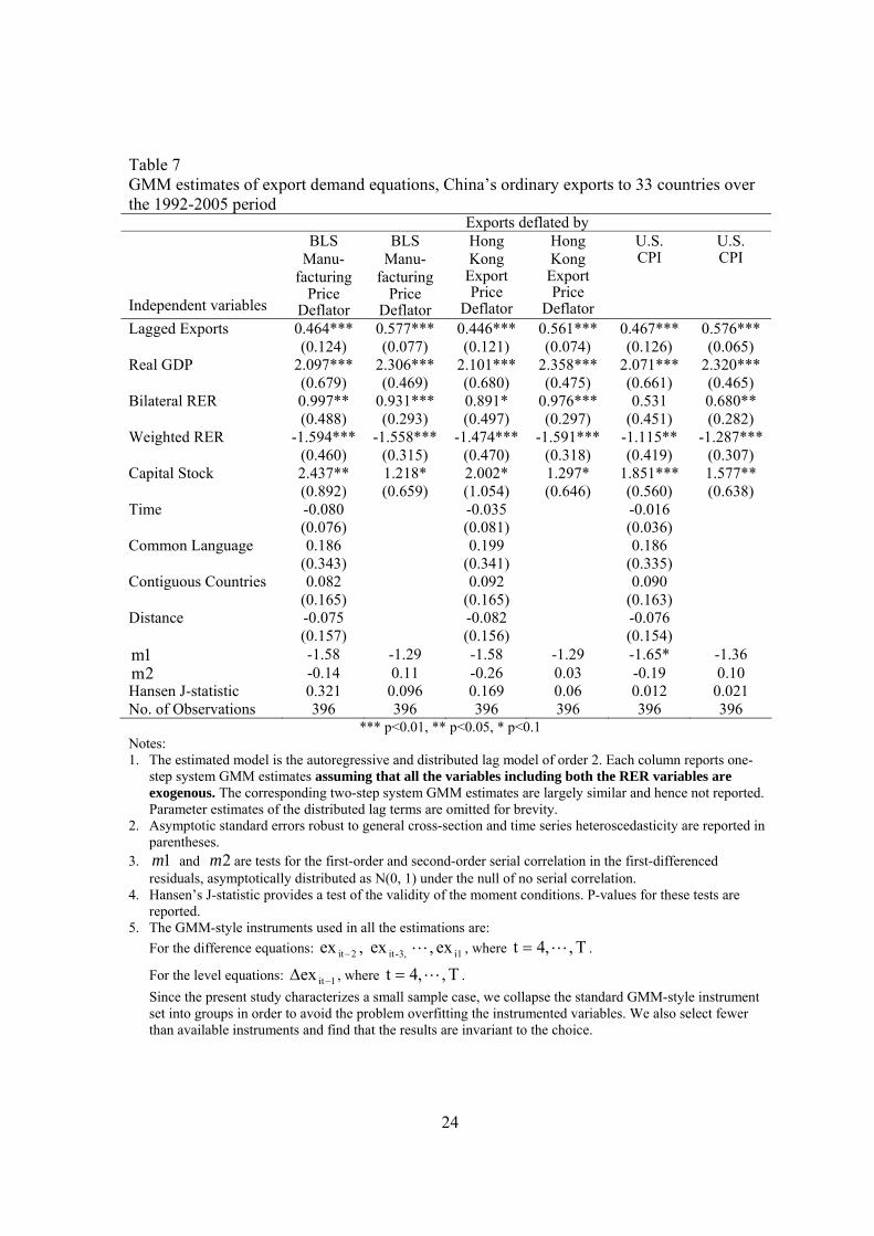
Table 7 GMM estimates of export demand equations, China’s ordinary exports to 33 countries over the 1992-2005 period Exports deflated by Independent variables
BLS Manu-
facturing Price
Deflator
BLS Manu-
facturingPrice
Deflator
Hong Kong
Export Price
Deflator
Hong Kong Export Price
Deflator
U.S. CPI
U.S. CPI
Lagged Exports 0.464*** 0.577*** 0.446*** 0.561*** 0.467*** 0.576*** (0.124) (0.077) (0.121) (0.074) (0.126) (0.065) Real GDP 2.097*** 2.306*** 2.101*** 2.358*** 2.071*** 2.320*** (0.679) (0.469) (0.680) (0.475) (0.661) (0.465) Bilateral RER 0.997** 0.931*** 0.891* 0.976*** 0.531 0.680** (0.488) (0.293) (0.497) (0.297) (0.451) (0.282) Weighted RER -1.594*** -1.558*** -1.474*** -1.591*** -1.115** -1.287*** (0.460) (0.315) (0.470) (0.318) (0.419) (0.307) Capital Stock 2.437** 1.218* 2.002* 1.297* 1.851*** 1.577** (0.892) (0.659) (1.054) (0.646) (0.560) (0.638) Time -0.080 -0.035 -0.016 (0.076) (0.081) (0.036) Common Language 0.186 0.199 0.186 (0.343) (0.341) (0.335) Contiguous Countries 0.082 0.092 0.090 (0.165) (0.165) (0.163) Distance -0.075 -0.082 -0.076 (0.157) (0.156) (0.154)
1m -1.58 -1.29 -1.58 -1.29 -1.65* -1.36 2m -0.14 0.11 -0.26 0.03 -0.19 0.10
Hansen J-statistic 0.321 0.096 0.169 0.06 0.012 0.021 No. of Observations 396 396 396 396 396 396
*** p<0.01, ** p<0.05, * p<0.1 Notes: 1. The estimated model is the autoregressive and distributed lag model of order 2. Each column reports one-
step system GMM estimates assuming that all the variables including both the RER variables are exogenous. The corresponding two-step system GMM estimates are largely similar and hence not reported. Parameter estimates of the distributed lag terms are omitted for brevity.
2. Asymptotic standard errors robust to general cross-section and time series heteroscedasticity are reported in parentheses.
3. 1m and 2m are tests for the first-order and second-order serial correlation in the first-differenced residuals, asymptotically distributed as N(0, 1) under the null of no serial correlation.
4. Hansen’s J-statistic provides a test of the validity of the moment conditions. P-values for these tests are reported.
5. The GMM-style instruments used in all the estimations are: For the difference equations: i13,-it2it ex, ex ,ex L− , where T,,4t L= .
For the level equations: 1itex −Δ , where T,,4t L= . Since the present study characterizes a small sample case, we collapse the standard GMM-style instrument set into groups in order to avoid the problem overfitting the instrumented variables. We also select fewer than available instruments and find that the results are invariant to the choice.
25
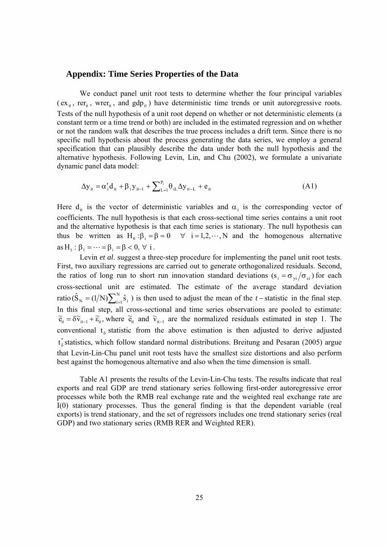
Appendix: Time Series Properties of the Data
We conduct panel unit root tests to determine whether the four principal variables ( itxe , iterr , itwrer , and itdpg ) have deterministic time trends or unit autoregressive roots. Tests of the null hypothesis of a unit root depend on whether or not deterministic elements (a constant term or a time trend or both) are included in the estimated regression and on whether or not the random walk that describes the true process includes a drift term. Since there is no specific null hypothesis about the process generating the data series, we employ a general specification that can plausibly describe the data under both the null hypothesis and the alternative hypothesis. Following Levin, Lin, and Chu (2002), we formulate a univariate dynamic panel data model:
∑ = −− +Δθ+β+α′=Δ iP
1L itLitiL1itiitiit eyydy (A1) Here itd is the vector of deterministic variables and iα is the corresponding vector of coefficients. The null hypothesis is that each cross-sectional time series contains a unit root and the alternative hypothesis is that each time series is stationary. The null hypothesis can thus be written as 0 :H i0 =β=β ∀ N,,2,1i L= and the homogenous alternative as ,0 :H i11 <β=β==β L ∀ i .
Levin et al. suggest a three-step procedure for implementing the panel unit root tests. First, two auxiliary regressions are carried out to generate orthogonalized residuals. Second, the ratios of long run to short run innovation standard deviations )s( iyii εσσ= for each cross-sectional unit are estimated. The estimate of the average standard deviation ratio ∑ =
=N
1i iN s)N1(S( ) is then used to adjust the mean of the statistic−t in the final step. In this final step, all cross-sectional and time series observations are pooled to estimate:
,~v~e~ it1itit ε+δ= − where ite~ and 1itv~ − are the normalized residuals estimated in step 1. The conventional δt statistic from the above estimation is then adjusted to derive adjusted
*t δ statistics, which follow standard normal distributions. Breitung and Pesaran (2005) argue that Levin-Lin-Chu panel unit root tests have the smallest size distortions and also perform best against the homogenous alternative and also when the time dimension is small.
Table A1 presents the results of the Levin-Lin-Chu tests. The results indicate that real
exports and real GDP are trend stationary series following first-order autoregressive error processes while both the RMB real exchange rate and the weighted real exchange rate are I(0) stationary processes. Thus the general finding is that the dependent variable (real exports) is trend stationary, and the set of regressors includes one trend stationary series (real GDP) and two stationary series (RMB RER and Weighted RER).
26
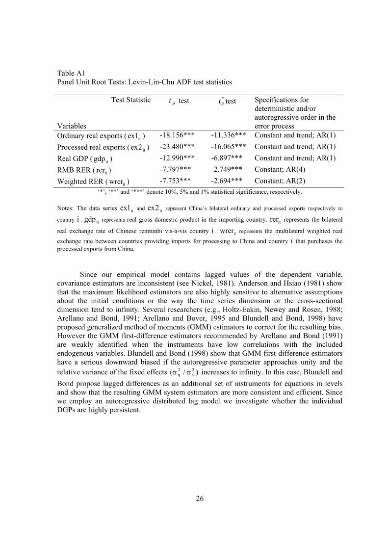
Table A1 Panel Unit Root Tests: Levin-Lin-Chu ADF test statistics
Test Statistic Variables
δt test *δt test Specifications for
deterministic and/or autoregressive order in the error process
Ordinary real exports ( it1ex ) -18.156*** -11.336*** Constant and trend; AR(1) Processed real exports ( it2ex ) -23.480*** -16.065*** Constant and trend; AR(1) Real GDP ( itgdp ) -12.990*** -6.897*** Constant and trend; AR(1) RMB RER ( itrer ) -7.797*** -2.749*** Constant; AR(4) Weighted RER ( itwrer ) -7.753*** -2.694*** Constant; AR(2)
‘*’, ‘**’ and ‘***’ denote 10%, 5% and 1% statistical significance, respectively. Notes: The data series it1ex and it2ex represent China’s bilateral ordinary and processed exports respectively to
country i . itgdp represents real gross domestic product in the importing country. itrer represents the bilateral
real exchange rate of Chinese renminbi vis-à-vis country i . itwrer represents the multilateral weighted real exchange rate between countries providing imports for processing to China and country i that purchases the processed exports from China.
Since our empirical model contains lagged values of the dependent variable, covariance estimators are inconsistent (see Nickel, 1981). Anderson and Hsiao (1981) show that the maximum likelihood estimators are also highly sensitive to alternative assumptions about the initial conditions or the way the time series dimension or the cross-sectional dimension tend to infinity. Several researchers (e.g., Holtz-Eakin, Newey and Rosen, 1988; Arellano and Bond, 1991; Arellano and Bover, 1995 and Blundell and Bond, 1998) have proposed generalized method of moments (GMM) estimators to correct for the resulting bias. However the GMM first-difference estimators recommended by Arellano and Bond (1991) are weakly identified when the instruments have low correlations with the included endogenous variables. Blundell and Bond (1998) show that GMM first-difference estimators have a serious downward biased if the autoregressive parameter approaches unity and the relative variance of the fixed effects )/( 2
v2 σση increases to infinity. In this case, Blundell and
Bond propose lagged differences as an additional set of instruments for equations in levels and show that the resulting GMM system estimators are more consistent and efficient. Since we employ an autoregressive distributed lag model we investigate whether the individual DGPs are highly persistent.
27
Persistency in the Individual DGPs
In order to assess the persistency of the individual variables, we estimate the univariate autoregressive model9
∑ = −− +Δθ+β+α′=Δ iP
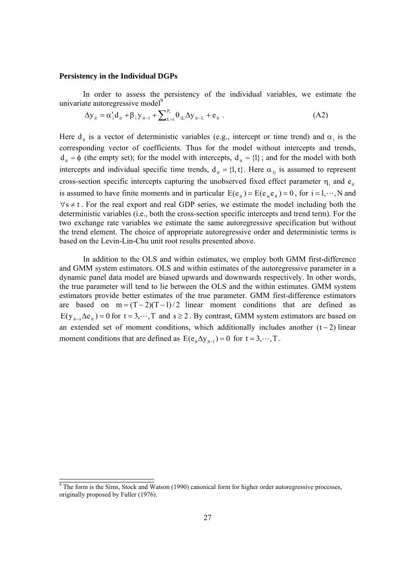
1L itLitiL1itiitiit eyydy . (A2) Here itd is a vector of deterministic variables (e.g., intercept or time trend) and iα is the corresponding vector of coefficients. Thus for the model without intercepts and trends,
φ=itd (the empty set); for the model with intercepts, }1{d it = ; and for the model with both intercepts and individual specific time trends, }.t,1{d it = Here i1α is assumed to represent cross-section specific intercepts capturing the unobserved fixed effect parameter iη and ite is assumed to have finite moments and in particular 0)ee(E)e(E itisit == , for N,,1i L= and
ts ≠∀ . For the real export and real GDP series, we estimate the model including both the deterministic variables (i.e., both the cross-section specific intercepts and trend term). For the two exchange rate variables we estimate the same autoregressive specification but without the trend element. The choice of appropriate autoregressive order and deterministic terms is based on the Levin-Lin-Chu unit root results presented above.
In addition to the OLS and within estimates, we employ both GMM first-difference
and GMM system estimators. OLS and within estimates of the autoregressive parameter in a dynamic panel data model are biased upwards and downwards respectively. In other words, the true parameter will tend to lie between the OLS and the within estimates. GMM system estimators provide better estimates of the true parameter. GMM first-difference estimators are based on 2/)1T)(2T(m −−= linear moment conditions that are defined as
0)ey(E itsit =Δ− for T,,3t L= and 2s ≥ . By contrast, GMM system estimators are based on an extended set of moment conditions, which additionally includes another )2t( − linear moment conditions that are defined as 0)ye(E 1itit =Δ − for T,,3t L= .
9 The form is the Sims, Stock and Watson (1990) canonical form for higher order autoregressive processes, originally proposed by Fuller (1976).

28
Table A2 presents our results. The evidence indicates that, while ordinary and processed exports are both trend stationary series, they are highly persistent. These results imply that GMM first-difference estimators are likely to be weakly identified and hence inconsistent. The findings instead suggest that our multivariate dynamic panel data model should exploit the extended instrument matrix proposed by Blundell and Bond (1998) and utilize GMM system estimators. Table A2 Estimates of the autoregressive parameter of individual data generation processes (DGPs) Name of the DGPs OLS GMM-Sys Within GMM-DiffOrdinary real exports ( it1ex ) 0.978*** 0.928*** 0.719*** 0.811*** (0.013) (0.043) (0.063) (0.091) Processed real exports ( it2ex ) 0.979*** 0.912*** 0.754*** 0.360*** (0.009) (0.027) (0.060) (0.097) Real GDP ( itgdp ) 0.997*** 0.974*** 0.771*** 0.521*** (0.001) (0.008) (0.043) (0.157) RMB RER ( itrer ) 0.999*** 0.786*** 0.282*** -0.070 (0.018) (0.081) (0.094) (0.132) Weighted RER ( itwrer ) 1.003*** 0.699*** 0.653*** 0.356* (0.016) (0.111) (0.092) (0.184)
Notes: *** p<0.01, ** p<0.05, * p<0.1 Notes: The data series it1ex and it2ex represent China’s bilateral ordinary and processed exports respectively to
country i . itgdp represents real gross domestic product in the importing country. itrer represents the bilateral
real exchange rate of Chinese renminbi vis-à-vis country i . itwrer represents the multilateral weighted real exchange rate between countries providing imports for processing to China and country i that purchases the processed exports from China. Moment Conditions and the Instrument Matrix
In Tables 2-5 we assume that rer and wrer are predetermined and that the other right hand side variables are exogenous. Let it,1x represent the predetermined variables and it,2x represent the exogenous variables. Here ) wrerrer( ititit,1 =′x and ) K gdp( iitit zx it2, ′=′ . The variables are described in the text. The moment conditions for the autoregressive and distributed lag (ADL) model of order 2 are defined as follows: i. For the difference equations: 0)uy(E itsit =Δ− , 0)u(E it,1 =Δ′ +− 1sitx and 0)ux(E iti,2 =Δ′Δ for
T,,4t L= and 2s ≥ , where ) ( iT,24i,2i,2 xxx ′′=′ L and ii. For the level equations: 0)uy(E it1it =Δ − , 0)u(E it,1 =′Δ itx , and 0)ux(E itit,2 =′ for T,,4t L= .
29
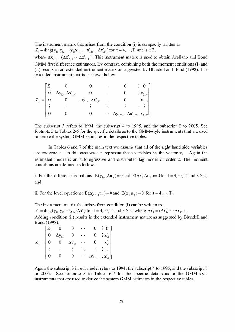
The instrument matrix that arises from the condition (i) is compactly written as )y y y(diagZ i,21is,11i,1isi21ii xxx ′Δ′′= + MLL for T,,4t L= and 2s ≥ .
where ) ( iT,24i,2i,2 xxx ′Δ′Δ=′Δ L . This instrument matrix is used to obtain Arellano and Bond GMM first difference estimators. By contrast, combining both the moment conditions (i) and (ii) results in an extended instrument matrix as suggested by Blundell and Bond (1998). The extended instrument matrix is shown below:
⎥⎥⎥⎥⎥⎥
⎦
⎤
⎢⎢⎢⎢⎢⎢
⎣
⎡
′
′′
′ΔΔ
′ΔΔ
′ΔΔ
=
−
+
iT,2
5i,2
4i,2
iT1,1T,i
i51,4i
i41,3i
i
i
0
. y000
0 y0000 y0000Z
Z
x
xx
x
xx
MM
M
M
L
MOMMM
L
L
L
The subscript 3 refers to 1994, the subscript 4 to 1995, and the subscript T to 2005. See footnote 5 to Tables 2-5 for the specific details as to the GMM-style instruments that are used to derive the system GMM estimates in the respective tables.
In Tables 6 and 7 of the main text we assume that all of the right hand side variables
are exogenous. In this case we can represent these variables by the vector itx . Again the estimated model is an autoregressive and distributed lag model of order 2. The moment conditions are defined as follows: i. For the difference equations: 0)uy(E itsit =Δ− and 0)ux(E itit =Δ′Δ for T,,4t L= and 2s ≥ , and ii. For the level equations: 0)uy(E it1it =Δ − and 0)ux(E itit =′ for T,,4t L= . The instrument matrix that arises from condition (i) can be written as:
)y y y(diagZ iisi21ii x′Δ= ML for T,,4t L= and 2s ≥ , where ) ( iT4ii xxx ′Δ′Δ=′Δ L . Adding condition (ii) results in the extended instrument matrix as suggested by Blundell and Bond (1998):
⎥⎥⎥⎥⎥⎥
⎦
⎤
⎢⎢⎢⎢⎢⎢
⎣
⎡
′
′′
Δ
ΔΔ
=
−
+
iT
5i
4i
1T,i
4i
3i
i
i
0
.y000
0y0000y0000Z
Z
x
xx
MM
M
M
L
MOMMM
L
L
L
Again the subscript 3 in our model refers to 1994, the subscript 4 to 1995, and the subscript T to 2005. See footnote 5 to Tables 6-7 for the specific details as to the GMM-style instruments that are used to derive the system GMM estimates in the respective tables.