Finance and Economics Discussion SeriesDivisions of Research & Statistics and Monetary Affairs

Federal Reserve Board, Washington, D.C.

How Useful are Estimated DSGE Model Forecasts

Rochelle M. Edge and Refet S. Gurkaynak

2011-11

NOTE: Staff working papers in the Finance and Economics Discussion Series (FEDS) are preliminarymaterials circulated to stimulate discussion and critical comment. The analysis and conclusions set forthare those of the authors and do not indicate concurrence by other members of the research staff or theBoard of Governors. References in publications to the Finance and Economics Discussion Series (other thanacknowledgement) should be cleared with the author(s) to protect the tentative character of these papers.

How Useful are Estimated DSGE Model Forecasts?∗

Rochelle M. EdgeFederal Reserve Board

Refet S. GurkaynakBilkent University

January 18, 2011

Abstract

DSGE models are a prominent tool for forecasting at central banks and the competitive

forecasting performance of these models relative to alternatives–including official forecasts–has

been documented. When evaluating DSGE models on an absolute basis, however, we find that

the benchmark estimated medium scale DSGE model forecasts inflation and GDP growth very

poorly, although statistical and judgmental forecasts forecast as poorly. Our finding is the DSGE

model analogue of the literature documenting the recent poor performance of macroeconomic

forecasts relative to simple naive forecasts since the onset of the Great Moderation. While this

finding is broadly consistent with the DSGE model we employ–ie, the model itself implies that

under strong monetary policy especially inflation deviations should be unpredictable–a “wrong”

model may also have the same implication. We therefore argue that forecasting ability during

the Great Moderation is not a good metric to judge the usefulness of model forecasts.

∗We are grateful to Burcin Kısacıkoglu for outstanding research assistance that went beyond the call of duty. Wethank Harun Alp, Selim Elekdag, Jeff Fuhrer, Marvin Goodfriend, Fulya Ozcan, Jeremy Rudd, Frank Smets, PeterTulip, Raf Wouters, and Jonathan Wright as well as seminar participants at Bilkent, the Brookings Panel, CentralBank of Turkey, Geneva Graduate Institute, GWU, Johns Hopkins, METU and PSE for very useful comments andsuggestions. We thank Ricardo Reis, David Romer, Chris Sims and Justin Wolfers for several rounds of detailedfeedback and also thank Volker Wieland and Maik Wolters for allowing us to cross check our data with theirs.This paper uses Blue Chip Economic Indicators and Blue Chip Financial Forecasts: Blue Chip Economic Indicatorsand Blue Chip Financial Forecasts are publications owned by Aspen Publishers. Copyright (C) 2010 by AspenPublishers, Inc. All rights reserved. http://www.aspenpublishers.com. The views expressed here are our own and donot necessarily reflect the views of the Board of Governors or the staff of the Federal Reserve System.

1 Introduction

Dynamic stochastic general equilibrium (DSGE) models were descriptive tools at their inception.

They were useful because they allowed economists to think about business cycles and carry out

hypothetical policy experiments in Lucas critique proof frameworks. In their early form, however,

they were viewed as too minimalistic to be appropriate for use in any practical application–such as

macroeconomic forecasting–for which a strong connection to the data was needed.

The seminal work of Smets and Wouters (2003, 2007), however, changed this perception. In

particular, their demonstration of the possibility of estimating a much larger and richly-specified

DSGE model (similar to that developed by Christiano, Eichenbaum, and Evans, 2005) as well as

their finding of a good forecast performance of their DSGE model relative to competing VAR

and Bayesian VAR (BVAR) models led DSGE models to be taken more seriously by central

bankers around the world. Indeed, estimated DSGE models are now quite prominent tools for

macroeconomic analysis at many policy institutions with forecasting being one of the key areas

where these models are used, in conjunction with other forecasting methods.

Reflecting this use of DSGE models, several central-bank modeling teams have in recent research

evaluated the relative forecasting performance of their institutions’ estimated DSGE models.

Notably, in addition to considering their DSGE models’ forecasts relative to time series models such

as BVARs (as Smets and Wouters did), these papers also consider official central bank forecasts.

For the U.S., Edge, Kiley, and Laforte (2010) compare the Federal Reserve Board’s DSGE model’s

forecasts to alternatives such as those generated in pseudo real time by time series models as well

as official Greenbook forecasts and find that the DSGE model forecasts are competitive with, and

indeed often better than, others.1 This is an especially notable finding given that previous analyses

have documented the high quality of the Federal Reserve’s Greenbook forecasts (Romer and Romer,

2000, Sims, 2002).

We began writing this paper with the aim of establishing the marginal contributions of

statistical, judgmental and DSGE model forecasts to efficient forecasts of key macroeconomic

variables, such as GDP growth and inflation. “How much importance should central bankers

attribute to model forecasts on top of judgmental or statistical forecasts?” was the question we

wanted to answer. To do this, we first evaluated the forecasting performance of the Smets-

Wouters (2007) model–a popular benchmark–for U.S. GDP growth, inflation and interest rates, and

compared these forecasts to those of a BVAR and the FRB staff’s Greenbook forecasts. Importantly,

1Other examples with similar findings include, Adolfson et al. (2007) for the Riksbank’s DSGE model and Leeset al. (2007) for the RBNZ’s DSGE model. In addition, Adolfson et al. (2006) and Christoffel et al. (2010) examineout-of-sample forecast performance for DSGE models of the euro area although the focus of these papers is muchmore on technical aspects of model evaluation.

2

to ensure that the same information is used to generate our DSGE model and BVAR model forecasts

as was used to formulate the Greenbook forecasts, we used real time data and re-estimated the

model at each Greenbook forecast date.

In line with the results in the DSGE model forecasting literature, we found that the root mean

squared errors (RMSEs) of the DSGE-model forecasts were similar to, and often better than, those

of the BVAR and Greenbook forecasts. Our surprising finding was that unlike what one would

expect when told that the model forecast is better than that of the Greenbook, the DSGE model in

an absolute sense did a very poor job of forecasting. The Greenbook and time series model forecasts

similarly did not capture much of the realized changes in GDP growth and inflation in our sample,

1992 to 2004. There is a moderate amount of nowcasting ability and then almost nothing beginning

with one quarter ahead forecasts. Thus, the forecast comparison is not one of one good forecast

relative to another; all three methods of forecasting are poor and combining them does not lead to

much improvement either.

This finding reflects the changed nature of macroeconomic fluctuations in the Great Moderation

period. For example, Stock and Watson (2007) have shown that since the Great Moderation, the

permanent (forecastable) component of inflation, which had earlier dominated, has diminished

such that the inflation process more recently has been largely influenced by the transitory

(unforecastable) component. An analogous point for GDP has been made by Tulip (2009). Data

availability prevents us from answering the question of whether the forecasting ability of estimated

DSGE models has worsened with the Great Moderation. We do, however, address the question of

whether these models’ forecasting performance are in an absolute sense poor and we find that they

are.

A key point we make in this paper is that forecasting ability is not always a good criteria for

a model’s success. As we discuss in more detail below, DSGE models of the class we consider

often imply that under a strong monetary policy rule there should not be much forecastability. In

other words, when there is not much to be forecasted in the observed out of sample data, as is the

case in the Great Moderation period, a “wrong” model will fail to forecast, but so will a “correct”

model. Consequently, it is entirely possible that a model that is unable to forecast, say inflation,

will nonetheless provide reasonable counterfactual scenarios, which is ultimately the main purpose

of the DSGE models.

The remainder of the paper is organized as follows. Section two describes the different

forecasting methods that we will consider in this paper, including those generated by the Smets

and Wouters (2007) DSGE model, the Bayesian VAR model, the Greenbook, and the Blue Chip

consensus forecast. The Blue Chip is an additional forecast that we consider primarily because

there is a five-year delay in the public release of Greenbook forecasts and we want to consider the

3

most recent recession. Section three then describes the data that we use, which as noted is real-

time to ensure that the same information is used to generate our DSGE model and BVAR model

forecasts as was used to formulate the Greenbook and Blue Chip forecasts. Section four describes

and presents the results for our forecast comparison exercises while section five discusses them.

Section six considers robustness analysis and extensions. In particular we show in this section that

judgmental forecasts have adjusted faster to capture the developments during the Great Recession.

Section seven concludes.

A contribution of this paper is the construction of real-time data sets using data vintages

that match Greenbook forecast dates and Blue Chip forecast dates. The appendix describes the

construction of this data in detail.2

2 Forecast Methods

In this section we briefly review the four different forecasts that we will later consider. These

forecasts are a DSGE model forecast, a Bayesian VAR model forecast, the Federal Reserve Board’s

Greenbook forecast, and the Blue Chip Consensus forecast.

2.1 DSGE Model

The DSGE model that we use in this paper is exactly that of Smets and Wouters (2007) and the

description of the model given here quite closely follows the description presented in section one of

Smets and Wouters (2007) and section two of Smets and Wouters (2003).

The Smets and Wouters model is an application of a real business cycle model (in the spirit of

King, Plosser, and Rebelo, 1988) to an economy with sticky prices and sticky wages. In addition

to nominal rigidities, the model also contains a large number of real rigidities–specifically habit

formation in consumption, costs of adjustment in capital accumulation, and variable capacity

utilization–that ultimately appear to be necessary to capture the empirical persistence of U.S.

macroeconomic data.

The model consists of households, firms, and a monetary authority. Households maximize a

non-separable utility function with goods and labor effort as its arguments over an infinite life

horizon. Consumption enters the utility function relative to a time-varying external habit variable

and labor is differentiated by a union. This assumed structure of the labor market enables the

household sector to have some monopoly power over wages. This implies a specific wage-setting

2All of the data used in this paper, except the Blue Chip median forecasts which are proprietary, are available athttp://www.bilkent.edu.tr//refet/research.html

4

equation that in turn allows for the inclusion of sticky nominal wages, modeled following Calvo

(1983). Capital accumulation is undertaken by households, who then rent capital to economy’s

firms. In accumulating capital households face adjustment costs, specifically investment adjustment

costs. As the rental price of capital changes, the utilization of capital can be adjusted, albeit at an

increasing cost.

The firms in the model rent labor and capital from households (in the former case via a union)

to produce differentiated goods for which they set prices, with Calvo (1983) price stickiness. These

differentiated goods are aggregated into a final good by different (perfectly competitive) firms in

the model and it is this good that is used for consumption and accumulating capital.

The Calvo model in both wage and price setting is augmented by the assumption that prices

that are not reoptimized are partially indexed to past inflation rates. Prices are therefore set in

reference to current and expected marginal costs but are also determined, via indexation, by the

past inflation rate. Marginal costs depend on the wage and the rental rate of capital. Wages are

set analogously as a function of current and expected marginal rates of substitution between leisure

and consumption and are also determined by the past wage inflation rate due to indexation. The

model assumes a variant of Dixit-Stiglitz aggregation in the goods and labor markets following

Kimball (1995). This aggregation allows for time-varying demand elasticities, which allows more

realistic estimates of price and wage stickiness.

Finally, the model contains seven structural shocks, which is equal to the number of observables

used in estimation. The model’s observable variables are the log difference of real per capita GDP,

real consumption, real investment, real wage, log hours worked, log difference of the GDP deflator,

and the federal funds rate. These series, and in particular their real time sources, are discussed in

detail below.

In estimation, the seven observed variables are mapped into 14 model variables by the Kalman

filter. Then 36 parameters (17 of which belong to the seven ARMA shock processes in the model)

are estimated via Bayesian methods (while 5 parameters are calibrated). It is the combination

of the Kalman filter and Bayesian estimation which allows this large (although technically called

a medium scale) model to be estimated rather than calibrated. In estimation we use exactly the

same priors as Smets and Wouters (2007) as well as using the same data series. Once the model

is estimated for a given data vintage, forecasting is done by employing the posterior modes for

each parameter. The model can produce forecasts for all model variables but we only use the GDP

growth, inflation and interest rate forecasts.

5

2.2 Bayesian VAR

The Bayesian VAR is, in its essence, a simple forecasting VAR(4). The same seven observable series

that are used in the DSGE model estimation are used in the VAR. Having seven variables in a four

lag VAR leads to a large number of parameters to be estimated which leads to over-fitting and poor

out-of-sample forecast performance problems. The solution is the same as for the DSGE model.

Priors are assigned to each parameter (and the priors we use are again those of Smets and Wouters,

2007) and the data are used to update these in the VAR framework. Similar to the DSGE model,

the BVAR is estimated at every forecast date using real time data and forecasts are obtained by

utilizing the modes of the posterior densities for each parameter.

Both the judgmental forecast and the DSGE model have an advantage over the purely statistical

model, the BVAR, in that the people who produce the Greenbook and Blue Chip forecasts obviously

know a lot more than seven time series and the DSGE model was built to match the data that is

being forecast. That is, judgment also enters the DSGE model in the form of modeling choices. To

help the BVAR overcome this handicap it is customary to have a training sample–to estimate the

model with some data and use the posteriors as priors in the actual estimation. Following Smets

and Wouters (2007) we also “trained” the BVAR with data from 1955-1965 but, in an a sign of how

different the early and the late parts of the sample are, found that the performance of the trained

and untrained BVAR are comparable. We therefore report results from the untrained BVAR only.

2.3 Greenbook

The Greenbook forecast is a detailed judgmental forecast that until March 2010 (after which it

became known as the Tealbook) was produced eight times a year by staff at the Board of Governors.3

The specific dates of when each Greenbook forecast is produced – and hence the data availability

of each round – is somewhat irregular since the Greenbook is made specifically for each Federal

Open Market Committee (FOMC) meeting and the timings of FOMC meetings are themselves

somewhat irregular. Broadly speaking FOMC meetings take place at an approximate six-week

interval (although they tend to be further apart at the beginning of the year and closer together at

the end of the year). The Greenbook is generally closed about one week before the FOMC meeting

takes place so as to allow FOMC members, and their staffs, enough time to review, analyze and

critique the document. Importantly–and unlike several other central banks–the Greenbook forecast

reflects the view of the staff and not the members of the FOMC.

Greenbook forecasts are formulated subject to a set of assumed paths for financial variables,

3The renaming of the Federal Reserve Board’s main forecasting document reflected a reorganization andcombination and the original Greenbook and Bluebook. Throughout this paper we will continue to refer to theFRB’s main forecasting document as the Greenbook.

6

such as the policy rate, key interest rates, and stock market wealth. Over time there has been

some variation in the way these assumptions have been set. For example, as can be seen from the

Greenbook federal funds rate assumptions reported in the Philadelphia Fed’s Real-Time Data Set

for Macroeconomists, from about the middle of 1990 to the middle of 1992 an essentially constant

path of the federal funds rate was assumed in making the forecast.4 In other periods, however, the

path of the federal funds rate does vary, reflecting a conditioning assumption about the path of

monetary policy consistent with the forecast.

As is the case for most judgmental forecasts, the maximum projection horizon for the Greenbook

forecast vintages is not constant and varies from ten to six quarters depending on the forecast round.

The July/August round of each year has the shortest projection horizon of any forecast round. It

extends six quarters: The current (third) quarter and the next (fourth) quarter and all four quarters

of the following year. In the September round of each year, the staff extend the forecast to include

the year following the next in the projection period. Since the third quarter is not yet finished

at the time of the September forecast, that quarter is still included in the Greenbook projection

horizon and so in total the horizon is ten quarters–the longest horizon for any forecast round.

The end-point of the projection horizon remains fixed for subsequent forecasts as the starting point

moves forward. This leaves the July/August forecast round with only a six-quarter forecast horizon.

In our analysis, we consider a maximum forecast horizon of eight quarters because the number of

observations for nine and ten quarters is very small. Of course, the number of observations for

a forecast horizons of seven and eight quarters (which we do consider) will be smaller than the

number of observations for horizons of six quarters and less.

We use the forecasts produced for the FOMC meetings starting in January 1992 and ending

in December 2004. Our forecast-vintage start date represents when the GDP, rather than GNP,

became the key indicator of economic activity. This is not a critical limitation since GNP forecasts

can clearly be used for earlier vintages. The end date was chosen by necessity: Greenbook forecasts

are made public only with a 5-year lag. The first two columns in Appendix Tables 1 to 13 provide

detailed information on the dates of Greenbook forecasts we use and the horizons covered in each

forecast. Note that the first four Greenbook forecasts that we consider fall in the episode of when

the policy rate was assumed to remain flat throughout the projection period.

2.4 Blue Chip

The Blue Chip Economic Indicators are a monthly poll of the forecasts for U.S. economic growth,

inflation, interest rates, and a range of other key variables of approximately 50 banks, corporations,

and consulting firms. The Blue Chip poll is taken on about the 4th or 5th of the month and the

4See http://www.philadelphiafed.org/research-and-data/real-time-center/greenbook-data/.

7

forecasts are published on the 10th day of each month. A consensus forecast, which is equal to the

median of the individual reported forecasts, is then reported along with the average of the top 10

and bottom 10 forecasts for each variable. In our analysis we use only the consensus forecast.

As with the Greenbook, the Blue Chip forecast horizons are not constant across forecast rounds

and in the case of the Blue Chip the forecast horizons are uniformly shorter. The longest forecast

horizon in the Blue Chip is nine quarters. This is for the January round for which a forecast is

made for the year to come and the next one, but for which the forth quarter of the previous year

is not yet available and is also “forecast.” The shortest forecast horizon in the Blue Chip is five

quarters. This is for the November and December rounds for which a forecast is made for the

current (fourth) quarter and the following year.

We use the Blue Chip consensus forecasts over the period January 1992 to September 2009.

The start date for the Blue Chip corresponds to the start date for the Greenbook. The end date is

one year prior to the time of writing.

3 Data and Sample

In this section we provide a brief overview of the data involved in the forecasting process and

our sample period. A detailed appendix presents sources and information on how the raw data is

converted to the form used in estimation.

The data we use for the estimation of the Smets-Wouters DSGE model and the BVAR model

are the same seven series used by Smets and Wouters (2007) but pulled for the real time vintages

of each series at each forecast date. Our forecast dates coincide with either the dates of Greenbook

forecasts or those of the Blue Chip forecasts. That is, at each Greenbook or Blue Chip forecast date,

we use the data that was available on that date to estimate the DSGE model and the BVAR.5 We

then generate forecasts out to eight quarters. From the data perspective, the last known quarter is

the previous one, therefore the one quarter ahead forecast is the nowcast (and the n quarter ahead

forecast corresponds to n− 1 quarters ahead counting from the forecast date.). This convention is

also the case for Greenbook and most Blue Chip forecasts.6

We will evaluate the forecasts for real per capita GDP growth, GDP deflator inflation and the

5See the appendix for exceptions to this. There are a few instances where one of the variables from the lastquarter is not released yet on a Greenbook forecast date. In these instances we help the DGSE and BVAR forecastsby appending the FRB staff backcast of that data point to the time series. That said, in these circumstances we verifythat doing so does not influence our results by dropping these forecast observations from our analysis and re-runningour results.

6The exception for the Blue Chip forecasts are the January, April, July, and October forecasts. These typicallytake place so early in the quarter than no or little data for the preceding quarter is available. For these forecasts theprevious quarter is considered the nowcast.

8

short (policy) rate. GDP growth and inflation are in terms of non-annualized quarter-on-quarter

rates, while interest rates are in levels. Our main focus will be on inflation forecasts because this is

the forecast that is the most comparable across the different forecasting methods. The DSGE model

and the BVAR produce continuous (and in very recent periods negative) interest rate forecasts while

judgmental forecasts obviously factor in the discrete nature of the interest rate setting and the zero

nominal bound. Furthermore, the Blue Chip forecasts do not contain forecasts of the federal funds

rate and hence we cannot do robustness checks for the interest rates or use the longer sample for

this variable.

The issue about GDP growth is more subtle. The DSGE model is based on per capita values

and produces a per capita GDP growth forecast. The BVAR similarly uses and produces per capita

values. On the other hand, GDP growth itself is announced in aggregate terms and Greenbook

and Blue Chip forecasts are in terms of aggregate growth. Thus, one has to either convert the

aggregate growth rates to per capita values by dividing them by realized population growth rates,

or convert per capita values to aggregate forecasts by multiplying them with realized population

growth numbers.

The two methods should produce similar results and the fact that the model uses per capita

data should make little difference as population growth is a smooth series with little variance.

However, the population numbers reported by the Census Bureau and used by Smets and Wouters

(and work following them) has a number of extremely sharp spikes caused by census picking up

previously uncaptured population levels as well as CPS rebasings. The spikes are there because the

data is not revised backwards; that is, population growth is placed in the quarter that uncaptured

population is measured, not across any estimate of the quarters over which it more likely occurred.

In this paper we used the population series used by Smets and Wouters in estimating the model

because we realized the erratic behavior of the population series after our estimation and forecast

exercise was complete. (We estimate the model more than 300 times, which took about two months,

and did not have the time to re-estimate and re-forecast using the better population series.) We

note the violence this does to the model estimates and encourage future researchers to smooth the

population series before using that data to obtain per capita GDP. Here, we adjust the DSGE

model and BVAR forecasts using the realized future population growth numbers to make them

comparable to announced GDP growth rates and judgmental forecasts but we again note that this

is an imperfect adjustment which likely hurts the DSGE model and BVAR forecasts.7

7We also experimented with converting the realized aggregate GDP growth numbers and Blue Chip forecasts toper capita values using the realized population growth rates, and converting the Greenbook GDP growth forecastinto per capita values by using the Fed staff’s internal population forecast. This essentially gives Blue Chip forecastsperfect foresight about the population component of per capita GDP, helping it quite a lot in forecasting becausethe variance of the population series is high, and hurts the Greenbook GDP forecast a lot because the Fed staffpopulation growth estimate is a smooth series. Those results are available upon request.

9

We estimate the models (DSGE and BVAR) with data going back to 1965 and do the first

forecast on January 1992. The Greenbook forecasts are embargoed for five years, therefore our

last forecast is in 2004:Q4, forecasting the period out to 2006:Q3. There are two scheduled FOMC

meetings per quarter and thus all of our forecasts that are compared to the Greenbook are made

twice a quarter. This has consequences for correlated forecast errors, as explained in the next

section. For Blue Chip forecasts, the forecasting period ends in 2010:Q1, the last quarter for which

we know the realized values of variables of interest. Blue Chip forecasts are published monthly and

we produce a separate set of real time DSGE and BVAR model forecasts coinciding with the Blue

Chip publication dates.

We should note that, while not identical, our sample, 1992 to 2004 for Greenbook comparisons,

is similar to the ones used in previous studies of forecast ability of DSGE models, such as Smets-

Wouters (2007), who use 1990 to 2004, and Edge et al. (2010) who use 1996 to 2002. It is

also important to note again that the sample is in the Great Moderation period, after the long

disinflation was complete, and that most of the period corresponds to a particularly transparent

monetary policy making episode, with the FOMC signalling likely policy actions in the near future

with statements accompanying releases of interest rate decisions.

4 Forecast Comparison

We distinguish between two types of forecast evaluations. Given a variable to be forecasted, x, and

its h-period ahead forecast (made h-periods in the past) by method y, xhy , one can compute the

root mean square error of the real time forecasts

RMSExhy =

√√√√ 1

T

T∑t=1

(xt − xhy,t

)2. (1)

Comparing the root mean square errors across different forecast methods, a policy maker can then

choose the method with the smallest RMSE to use. The RMSE comparison therefore answers the

decision theory question: Which forecast is the best and should be used? To our knowledge, all of

the forecast evaluations of DSGE models so far (Smets and Wouters 2007, Edge et al. 2010, and

those mentioned earlier for other countries) have used essentially this metric–and concluded that

the model forecasts do well.

In Figure 1 we carry out this exercise with real time data and show the RMSE of the DSGE

model forecasts for inflation and GDP growth relative to those of the Greenbook and BVAR

forecasts at different horizons. This figure visually conveys a result that Smets and Wouters

and Edge et al. have shown earlier: except for very short horizon inflation forecasts (where the

10

Greenbook forecasts are better) the DSGE model forecasts have the lowest RMSE for both inflation

and growth. The literature has taken this finding as both a vindication of the estimated medium

scale DSGE model, and as a sign that these models can be used for forecasting as well as for positive

analysis of counterfactuals and for optimal policy questions.

While Figure 1 indeed shows that the DSGE model has the best forecasting record among the

three forecasting methods we consider, it does not offer any clues about how good the “best” is. To

further evaluate the forecasts, we first look in Figure 2 at the scatter plots of the four quarter ahead

forecasts (a horizon that the DSGE model outperforms the Greenbook and BVAR ) of inflation

and GDP growth from the DSGE model and the realized values of these variables. With a good

forecast performance, the observations should lie on the 45-degree line.

The scatter plots shown in Figure 2 are surprising. For both variables, the points form clouds

rather than 45-degree lines, suggesting that the four quarter ahead forecast of the DSGE model is

quite unrelated to the realized value. To get the full picture, we run a standard forecast efficiency

test (see Gurkaynak and Wolfers, 2007, for a discussion of tests of forecast efficiency and further

references) and estimate

xt = αhy + βhy x

hy,t + εhy,t. (2)

A “good” forecast should have an intercept of zero, a slope coefficient of one, and a high R2. If

the intercept is different from zero the forecast has on average been biased, if the slope is different

from one, the forecast has consistently under or over predicted deviations from the mean, and if the

R2 is low then little of the variation of the variable to be forecasted is captured by the forecast. Note

that especially when the point estimates of αhy and βhy are different from zero and one, respectively,

the R2 is a more charitable measure of the success of the forecast than the RMSE calculated in (1)

as the errors in (2) are residuals obtained from the best fitting line. That is, a policy maker would

make errors of size εhy,t only if she knew the values of αhy and βhy and adjusted xhy,t with these. The

R2 that is comparable to the RMSE measures calculated in (1) would be that implied by equation

(2) with αhy and βhy constrained to 0 and 1, respectively.

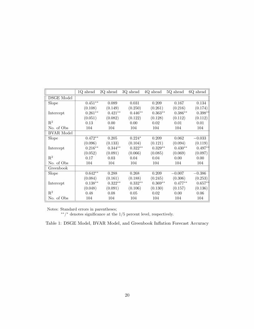
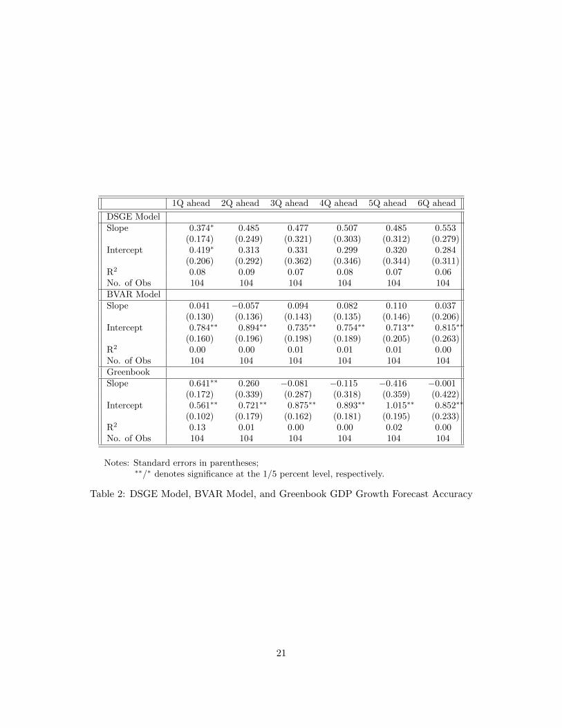
Tables 1 to 3 show the estimation results of (2) for the DSGE model, BVAR and Greenbook

forecasts of inflation, GDP growth and interest rates, respectively.8 The table suggests that

forecasts of inflation and GDP growth have been very poor by all methods, except for the Greenbook

inflation nowcast. The DSGE model inflation forecasts have about zero R2 for forecasts of the next

quarter and beyond, and slope coefficients very far away from unity. GDP growth forecasts are

likewise capturing less than 10 percent of the actual variation in growth and point estimates of the

8The standard errors reported are Newey-West standard errors for 2 ∗ h lags, given there are two forecasts madein each quarter. Explicitly taking the clustering at the level of quarters–as the forecasts made in the same quartermay be correlated–into account made no perceptible difference. Neither did using only the first or second forecast ineach quarter.

11

slopes are again away from unity. Except for the Greenbook nowcast, the results are very similar

for the judgmental forecast and the BVAR forecasts.

All three forecast methods, however, do impressively in forecasting interest rates (Table 3). This

is surprising as short rates should be a function of inflation and GDP, and thus should not be any

more forecastable than these two variables, except for the forecastability coming from interest rate

smoothing by policy makers. The issue here is that the interest rate is highly serially correlated,

which makes it easy to forecast. (Indeed, in our sample the level of the interest rate behaves like

a unit root process as verified by an unreported ADF test.)9 Thus, Table 3 is possibly showing

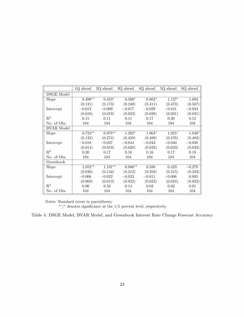
long-run cointegrating relationships rather than short-run forecasting ability. We therefore follow

Gurkaynak, Sack, and Swanson (2005) in studying at the change in the interest rate rather than

its level.

Table 4 shows the interest rate change forecast evaluations for the three methods. The forecast

success is now more comparable to inflation and GDP growth forecasts, although in the short run

there is quite high forecastability in interest rate changes. The very strong nowcasting ability of

the Greenbook partly comes from the fact that while the Fed staff know interest rates changes in

integer multiples of 25 basis points, while BVAR and the DSGE model produce continuous interest

rate forecasts.

The panels of Figure 2 and Tables 1 to 4 collectively show that while the DSGE model forecasts

are comparable and often better than Greenbook and BVAR forecasts, this is a comparison of very

poor forecasts to each other. To provide a benchmarks for forecast quality, we introduce a constant

and a random walk forecast and ask the following two questions. First, if a policy maker could

have used one of these three forecasts over the 1992-2006 period or could have access to the actual

mean of the series over the same period and used that as a forecast (and zero change as the interest

rate forecast at all horizons) how would the root mean square errors compare? Second, how large

would the root mean square errors be if the policy maker used the last observation on each date as

the forecast for all horizons, essentially treating the series to be forecast as random walks?10

We show the actual levels of the root mean square errors in Figure 3. The constant forecast does

about as well as the other forecasts, and often better, suggesting that the DSGE model, BVAR and

Greenbook forecasts are not accomplishing much. It is some relief, however, that the DSGE model

forecast usually does better than the random walk forecast, an often used benchmark.11 But notice

9While nominal interest rates cannot theoretically be simple unit root processes due to the zero nominal bound,they can be statistically indistinguishable from unit root processes in small samples and pose their econometricdifficulties.

10In the random walk forecasts we set the interest rate change forecasts to zero. That is, in this exercise theassumed policy maker treats the level of the intertest rate as a random walk.

11We also looked at how the DSGE model forecast RMSEs compare to other forecast RMSEs statistically (resultsavailable from the authors). The Diebold-Mariano test results show that for inflation the RMSE of the DGSE model

12

that the random walk RMSEs are very large. To understand the quantities involved, observe that

the 6-quarter ahead inflation forecast RMSE of the DSGE model is about 0.25 in quarterly terms.

This would be about one percent annualized and would lead to a 95 percent confidence interval

that is 4 percentage points wide. That is not very useful for policy making.

5 Discussion

Our findings are surprising, especially for inflation, given the Romer and Romer (2000) finding that

the Greenbook is an excellent forecaster of inflation at horizons out to eight quarters. Figure 4

shows the reason of the difference. The Romer and Romer sample covers a period when inflation

had a large swing. Our sample–and the sample used in other studies for DSGE model forecast

evaluations–covers a period where inflation behaves more as i.i.d. deviations around a constant

level. That is, there is little to be forecasted over our sample.

This finding is in line with Stock and Watson’s (2007) result that after the Great Moderation,

the permanent (forecastable) component of inflation, which had earlier dominated, diminished

in importance and the bulk of the variance of inflation began to be driven by the transitory

(unforecastable) component. It is therefore not surprising that no forecasting method does well.

Trehan (2010) shows that a similar lack of forecast ability is also evident in the Survey of Professional

Forecasters and the Michigan Survey. Atkeson and Ohanian (2001) document that over the period

1984 to 1999 a random-walk forecast of four-quarter ahead inflation outperforms the Greenbook

forecast as well as Phillips curve models. (But note that here we find that the DSGE model, with

a sophisticated microfounded Phillips curve, outperforms the random walk forecast.) Fuhrer et

al.(2009) show that this is due to the parameter changes in the inflation process that have occurred

with the onset of the Great Moderation. For forecasts of output growth, Tulip (2009) documents a

notably larger reduction in actual output growth volatility following the Great Moderation relative

to the reduction in Greenbook RMSEs, thus indicating that much of the reduction in output-growth

volatility has stemmed from the predictable component–that is, the part that can potentially be

forecast.

Reifschneider and Tulip (2009) perform a wide reaching analysis of institutional forecasts–

specifically, the Greenbook, the SPF and the Blue Chip, as well as forecasts produced by

the Congressional Budget Office and the Administration–for real GDP (or GNP) growth, the

unemployment rate, and CPI inflation. Although they do not consider changes in forecast

is significantly lower than those of the BVAR and the random walk forecasts for most maturities, is indistinguishablefrom the RMSE of the Greenbook and is higher than that of the constant forecast for some maturities; while for GDPgrowth the DSGE model RMSE is statistically lower than those of the BVAR and the random walk forecasts and isindistinguishable from the RMSEs of the Greenbook and the constant forecasts.

13

performance associated with the Great Moderation their analysis, which is undertaken for the

post-1986 period, finds overwhelmingly that errors for all institutional forecasts are large. More

broadly D’Agostino and Giannone (2006) also consider a range of time series forecasting models,

including univariate AR models, factor augmented AR models, and pooled bivariate forecasting

models, as well as institutional forecasts–that is, the Greenbook forecast and the forecasts from

the SPF–and document that while RMSEs for forecasts of real activity, inflation, and interest rates

have dropped notably with the Great Moderation, time series and institutional forecasts have also

largely lost their ability to improve on a random walk. Faust and Wright (2009) similarly note that

performances of some of the forecasting methods they consider improves when data from periods

preceding the Great Moderation is included in the sample.

We would argue that DSGE models should not be judged solely by their (lack of) absolute

forecast abilities. Previous authors, such as, Edge et. al (2010), were conscious of the declining

performance of Greenbook and time series forecasts when they performed their comparison exercises

but took as given the fact that staff at the Federal Reserve Board are required to produce forecasts

of the macroeconomy eight times a year. More precisely, they asked whether a DSGE model forecast

should be introduced into the mix of inputs used to arrive at the final Greenbook forecast. In this

case relative forecast performance is a relevant point of comparison. Another aspect of central bank

forecasting that is important to note is that of “story telling.” That is, not only are the values of

the forecast variables important but so too is the narrative explaining how present imbalances will

be unwound as the macroeconomy moves toward the balanced growth path. A well thought out

and much scrutinized story accompanies the Greenbook forecast but is not something present in

reduced-form time series forecasts. An internally consistent and coherent narrative is, however,

implicit in a DSGE model forecast, indicating that these models can also contribute along this

important dimension of forecasting.

In sum, what do these findings say about the quality of DSGE models as a tool for telling

internally consistent, reasonable stories for counterfactual scenarios? Not much. Inflation being

unforecastable is a prediction of basic sticky price DSGE models when monetary policy responds

aggressively to inflation. Goodfriend and King (2009) make this point explicitly using a tractable

model. If inflation is forecasted to be high, policy makers increase interest rates and rein in inflation.

Thus, inflation is never predictably different from the (implicit) target and all of the variation comes

from unforecastable shocks. In models lacking real rigidities the divine coincidence will be present,

which means that the output gap will have the same property of unforecastability. Thus, it is

well possible that the model is “correct” and therefore cannot forecast cyclical fluctuations but the

counterfactual scenarios produced by the model can still inform policy discussions.12

12Although see Gali (2010) about difficulties inherent in generating counterfactual scenarios using DSGE models.

14

Of course, the particular DSGE model we employ in this paper does not have the divine

coincidence due to the real rigidities it includes, such as a real wage rigidity due to having both sticky

prices and sticky wages. Moreover because in this model there is a trade-off between stabilizing price

inflation, wage inflation, and the output gap, optimal policy is not characterized by price-inflation

stabilization and therefore unforecastable price inflation. Nonetheless, price-inflation stabilization

is a possible policy, which could be pursued even if not optimal, and this would imply unforecastable

inflation. That said, this policy would likely not stabilize the output gap, so implying some

forecastability of the output gap. Ultimately, whether, and to what extent, the model implies

(un)forecastable fluctuations in inflation and GDP growth can be learned by simulating data from

the model calibrated under different monetary policy rules and performing forecast exercises on

the simulated data. We note the qualitative model implication that there should not be much

predictability, especially for inflation, and leave the quantitative study to future research. Note

also that our discussion here has focused on the forecastability of the output gap, not output

growth, which is ultimately the variable of interest in our forecast exercises. Unforecastability of

the output gap may not imply unforecastability of output growth.

Finally, we would note that a reduced form model with an assumed inflation process that is equal

to a constant with i.i.d. deviations–i.e. a “wrong” model–will also have the same unforecastability

implication. Thus evaluating forecasting ability during a period such as the Great Moderation,

when no method is able to forecast, is not a test of the empirical relevance of a model.

6 Robustness and Extensions

To verify that our results are not specific to the relatively short sample we have used and to the

Greenbook date vintages we employed, we repeated the exercise using Blue Chip forecasts as the

judgmental forecast for the 1992-2010 period. (This also has the advantage of adding the Great

Recession period to our sample.) We also estimated the DSGE model and the BVAR using data

vintages of Blue Chip publication dates and produced forecasts.

We do not display the analogues of Figures 1 to 3 and Tables 1 to 4 for brevity but note that the

findings are very similar when Blue Chip forecasts replace Greenbook forecasts and the sample is

extended to 2010, encompassing the financial crisis episode. (One difference is that the Blue Chip

forecast has nowcasting ability for GDP as well as inflation.) The DSGE model forecast is similar

to the judgmental forecast and is better than the BVAR in the RMSE sense for almost all horizons,

but all three forecasts are very poor forecasts. (This exercise omits the forecasts of interest rates as

Blue Chip does not include forecasts of the overnight rate.) The longer sample allows us to answer

some interesting questions and provide further robustness checks.

15

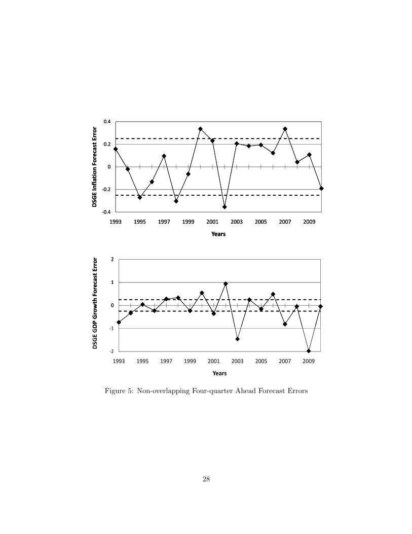
Although we use quarter over quarter changes and not annual growth rates for all of our

variables, overlapping periods in long horizon forecasting is a potential issue. In Figure 5 we

show the non-overlapping four quarter ahead absolute errors of DSGE model forecasts made in the

January of each year for the first quarter of the subsequent year. Horizontal lines at -0.25 and 0.25

show forecast errors that would be one percentage point in annualized terms. Most errors are near

or above (in absolute value) these bounds. It is clear that our statistical results are not driven by

outliers (a fact also visible in Figure 1).

To provide a better understanding of the evolution of forecast errors over time, Figure 6 shows

three year rolling averages of root mean square errors for four quarter ahead forecasts, using all

12 forecasts for each year. Not surprisingly, the forecast errors are considerably higher in the

latter part of the sample, which includes the crisis episode. The DSGE model does worse than the

Blue Chip forecast once the rolling windows includes 2008, for both inflation and the GDP growth

forecasts.

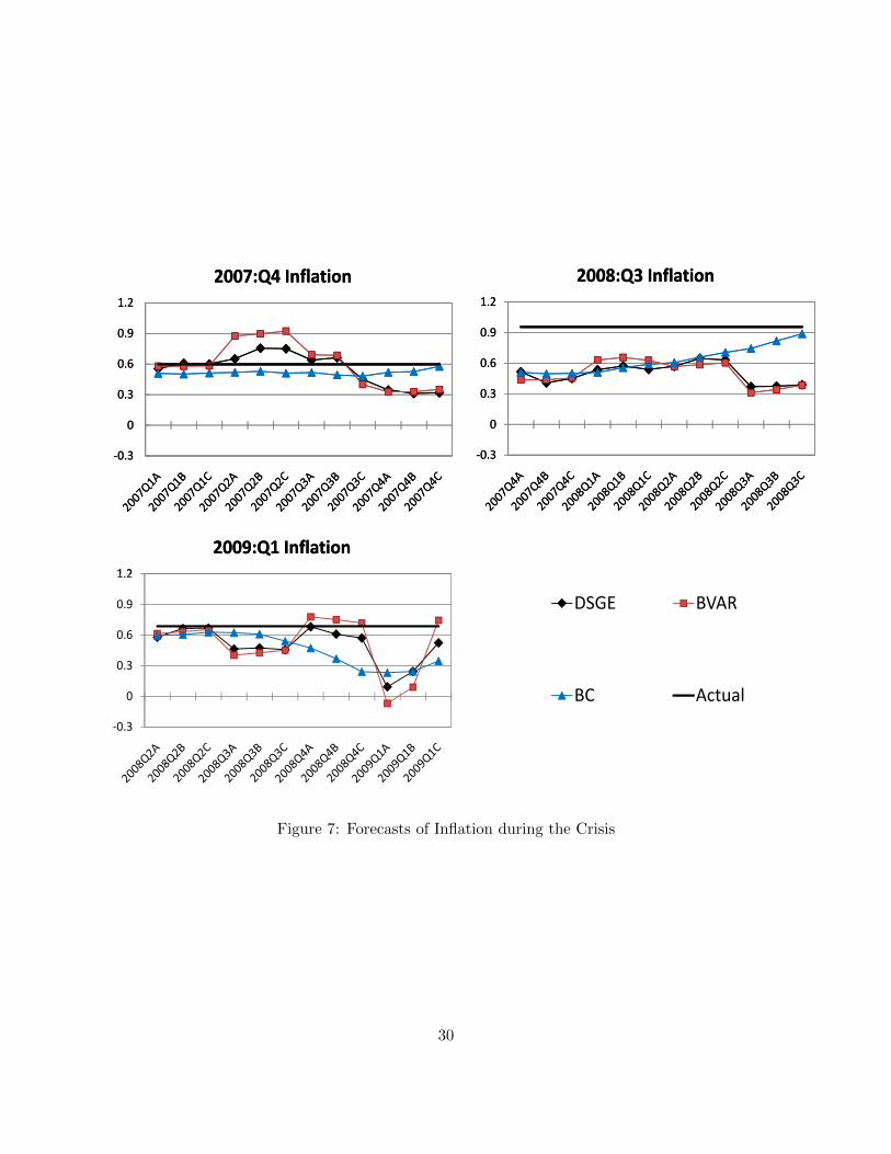
Lastly, we look at the forecasting performance of the DSGE and BVAR models compared to the

Blue Chip forecasts during the recent crisis and the recession. Figures 7 and 8 show the forecast

errors for inflation and GDP growth beginning with 4 quarter ahead forecasts and ending with the

nowcast for three quarters: 2007Q4, the first quarter of the recession according to the NBER dating,

2008Q3, when Lehman failed and per capita GDP growth turned negative, and 2009Q1, when the

extent of the contraction became clear (see Wieland and Wolters, 2010, for a similar analysis of

more episodes).13 A salient feature of all panels in Figures 7 and 8 is the closeness of the model

forecast and the judgmental forecast to each other when the forecast horizon is four quarters. While

all forecasts clearly first miss the recession, then its severity, the Blue Chip forecasts in general far

better when the quarter to be forecasted gets closer and especially when nowcasting.

An interesting point is the within quarter improvement in the judgmental forecast, especially

for the nowcast quarter, and the lack of a similar improvement for the DSGE and BVAR model

forecasts. The DSGE and statistical models have access to more revised versions of data belonging

to the previous quarter and before as the quarter progresses. On the other hand, forecasters

surveyed by the Blue Chip survey observe within quarter developments and learn of industrial

production, retail sales, etc. as well as receiving updates about policy responses, which were not

following previous prescriptions that are in the estimated parameters. For example, the Blue Chip

forecasters surely knew of the zero nominal bound, whereas both estimated models (DSGE and

statistical) imply deeply negative nominal rate forecasts during the crisis.

It is not very surprising that judgmental forecasts fare better in capturing such regime switches.

The DSGE model, lacking a financial sector and a zero nominal bound, should naturally do

13In the horizontal axis labels, (A), (B), and (C) denote the first, second, and third month of a given quarter.

16

somewhat better in the pre-crisis period. In fact, that is the period this model was built to explain.

But this also cautions us that out-of-sample tests for DSGE models are not truly out of sample as

long as the sample is in the period the model was built to explain. The next generation of DSGE

models will likely have the zero nominal bound and a financial sector as standard features and will

do better when explaining the great recession. Their real test will be to explain–but not necessarily

to forecast–the first business cycle that follows those models’ creation.14

7 Conclusion

DSGE models are very poor in forecasting, but so are all other approaches. Forecasting ability

is a nonissue in DSGE model evaluation because in recent samples (over which these models can

be evaluated using real time data) there isn’t much to be forecasted. This is consistent with the

literature on the Great Moderation, which emphasizes that not only the standard deviation of

macroeconomic fluctuations, but also their nature has changed. In particular, cycles are driven

more by temporary, unforecastable shocks.

The lack of forecastability is not, however, evidence against the DSGE model and indeed can

be evidence in favor of it. Monetary policy was characterized with a strongly stabilizing rule in

this period and the model implies that such policy will undo predictable fluctuations, especially in

inflation. We leave scrutinizing this point and studying the forecasting ability of the model in pre-

and post-Great Moderation periods in more detail to future work and conclude by repeating that

forecasting ability is not a proper metric to judge a model.

References

[1] Adolfson, M., M. Andersson, J. Linde, M. Villani, and A. Vredin. 2007. “Modern Forecasting

Models in Action: Improving Macroeconomic Analyses at Central Banks,” International

Journal of Central Banking 3(4), 111-144.

[2] Adolfson, M., J. Linde, and M. Villani. 2006. “Forecasting Performance of an Open Economy

Dynamic Stochastic General Equilibrium Model.” Sveriges Riksbank Working Paper Series,

No. 190.

[3] Atkeson, A. and L. Ohanian. 2001.“Are Phillips Curves Useful for Forecasting Inflation?,”

Quarterly Review, Federal Reserve Bank of Minneapolis (Winter), 2-11.

14A promising avenue of research is adding unemployment explicitly to the model, as in Gali, Smets and Wouters(2010). This will likely help improve the model forecasts as Stock and Watson (2010), show that utilizing anunemployment gap measure helps improve forecasts of inflation in recession episodes.

17

[4] Calvo, G. 1983. “Staggered Prices in a Utility-Maximizing Framework,” Journal of Monetary

Economics 12(3), 383-398.

[5] Christiano, L., M. Eichenbaum, and C. Evans. 2005. “Nominal Rigidities and the Dynamic

Effects of a Shock to Monetary Policy,” Journal of Political Economy 113(1), 1-45.

[6] Christoffel, K., G. Coenen, and A. Warne. 2010. “Forecasting with DSGE Models,” in M.

Clements and D. Hendry (eds), Handbook of Forecasting, Oxford University Press, Oxford,

forthcoming.

[7] D’Agostino, A. and D. Giannone. 2006. “Comparing Alternative Predictors Based on Large-

Panel Factor Models,” ECB Working Paper No. 680.

[8] Edge, R., M. Kiley, and JP. Laforte. 2010. “A Comparison of Forecast Performance between

Federal Reserve Staff Forecasts, Simple Reduced-Form Models, and a DSGE Model,” Journal

of Applied Econometrics, 25(4), 720-54.

[9] Faust, J. and J. Wright. 2009. “Comparing Greenbook and Reduced Form Forecasts Using a

Large Realtime Dataset,” Journal of Business and Economic Statistics 27(4), 468-479.

[10] Fuhrer, J., G. Olivei, and G. Tootell. 2009. “Empirical Estimates of Changing Inflation

Dynamics,” FRB Boston Working Paper No. 09-4.

[11] Gali, J. 2010. “Are Central Banks’ Projections Meaningful?” CEPR Discussion Paper 8027.

[12] Gali, J., F. Smets, and R. Wouters. 2010. “Unemployment in an Estimated New Keynesian

Model,” Working Paper, CREI.

[13] Goodfriend, M. and R. King. 2009. “The Great Inflation Drift,” NBER Working Paper No.

14862

[14] Gurkaynak, R., E. Swanson and B. Sack. 2005. “Market-Based Measures of Monetary Policy

Expectations,” Journal of Business and Economic Statistics 25(2), 201-12.

[15] Gurkaynak, R. and J. Wolfers. 2007. “Macroeconomic Derivatives: An Initial Analysis of

Market-Based Macro Forecasts, Uncertainty, and Risk,” NBER International Seminar on

Macroeconomics 2005 (2), 11-50.

[16] Kimball, M. 1995. “The Quantitative Analytics of the Basic Neomonetarist Model,” Journal

of Money, Credit, and Banking 27(4), 1241–1277

[17] King, R., C. Plosser, and S. Rebelo. 1988. “Production, Growth and Business Cycles I,”

Journal of Monetary Economics 21(2-3),195-232.

18

[18] Lees K., T. Matheson, and C. Smith. 2007. “Open Economy DSGE-VAR Forecasting and

Policy Analysis - Head to Head with the RBNZ Published Forecasts,” Reserve Bank of New

Zealand Discussion Paper No. 2007/01.

[19] Reifschneider, D. and P. Tulip. 2007. “Gauging the Uncertainty of the Economic Outlook from

Historical Forecasting Errors,” FEDS Working Paper 2007-60.

[20] Romer, C. and D. Romer. 2000. “Federal Reserve Information and the Behavior of Interest

Rates,” American Economic Review 90(3), 429-457.

[21] Sims, C. 2002. “The Role of Models and Probabilities in the Monetary Policy Process,”

Brookings Papers on Economic Activity 2002(2), 1-40.

[22] Smets, F. and R. Wouters. 2003. “An Estimated Stochastic Dynamic General Equilibrium

Model of the Euro Area,” Journal of European Economic Association, 1(5), 1123-1175.

[23] Smets, F. and R. Wouters. 2007. “Shocks and Frictions in US Business Cycles: A Bayesian

DSGE Approach,” American Economic Review 97(3), 586-607.

[24] Stock, J. and M. Watson. 2007. “Why Has U.S. Inflation Become Harder to Forecast?” Journal

of Money Credit and Banking 39(1), 3-33.

[25] Stock, J. and M. Watson. 2010. “Modeling Inflation after the Crisis,” Paper presented at the

Federal Reserve Bank of Kansas City Economic Policy Symposium.

[26] Trehan, B. 2010. “Survey Measures of Expected Inflation and the Inflation Process,” FRBSF

Working Paper Series No. 2009-10

[27] Tulip, P. 2009.“Has the Economy Become More Predictable? Changes in Greenbook Forecast

Accuracy,” Journal of Money, Credit and Banking 41(6), 1217-1231.

[28] Wieland, W. and M. Wolters. 2010. ‘The Diversity of Forecasts from Macroeconomic Models

of the U.S. Economy,” Working Paper, Goethe University.

19

1Q ahead 2Q ahead 3Q ahead 4Q ahead 5Q ahead 6Q ahead

DSGE ModelSlope 0.451∗∗ 0.089 0.031 0.209 0.167 0.134

(0.108) (0.149) (0.250) (0.261) (0.216) (0.174)Intercept 0.261∗∗ 0.421∗∗ 0.446∗∗ 0.363∗∗ 0.386∗∗ 0.398∗∗

(0.051) (0.082) (0.122) (0.128) (0.112) (0.112)R2 0.13 0.00 0.00 0.02 0.01 0.01No. of Obs 104 104 104 104 104 104BVAR ModelSlope 0.472∗∗ 0.205 0.224∗ 0.209 0.062 −0.033

(0.096) (0.133) (0.104) (0.121) (0.094) (0.119)Intercept 0.216∗∗ 0.344∗∗ 0.322∗∗ 0.329∗∗ 0.430∗∗ 0.497∗∗

(0.052) (0.091) (0.066) (0.085) (0.069) (0.097)R2 0.17 0.03 0.04 0.04 0.00 0.00No. of Obs 104 104 104 104 104 104GreenbookSlope 0.642∗∗ 0.288 0.268 0.209 −0.007 −0.386

(0.084) (0.161) (0.188) (0.245) (0.306) (0.253)Intercept 0.138∗∗ 0.322∗∗ 0.332∗∗ 0.369∗∗ 0.477∗∗ 0.657∗∗

(0.048) (0.091) (0.106) (0.130) (0.157) (0.136)R2 0.48 0.08 0.05 0.02 0.00 0.06No. of Obs 104 104 104 104 104 104

Notes: Standard errors in parentheses;∗∗/∗ denotes significance at the 1/5 percent level, respectively.

Table 1: DSGE Model, BVAR Model, and Greenbook Inflation Forecast Accuracy

20

1Q ahead 2Q ahead 3Q ahead 4Q ahead 5Q ahead 6Q ahead

DSGE ModelSlope 0.374∗ 0.485 0.477 0.507 0.485 0.553

(0.174) (0.249) (0.321) (0.303) (0.312) (0.279)Intercept 0.419∗ 0.313 0.331 0.299 0.320 0.284

(0.206) (0.292) (0.362) (0.346) (0.344) (0.311)R2 0.08 0.09 0.07 0.08 0.07 0.06No. of Obs 104 104 104 104 104 104BVAR ModelSlope 0.041 −0.057 0.094 0.082 0.110 0.037

(0.130) (0.136) (0.143) (0.135) (0.146) (0.206)Intercept 0.784∗∗ 0.894∗∗ 0.735∗∗ 0.754∗∗ 0.713∗∗ 0.815∗∗

(0.160) (0.196) (0.198) (0.189) (0.205) (0.263)R2 0.00 0.00 0.01 0.01 0.01 0.00No. of Obs 104 104 104 104 104 104GreenbookSlope 0.641∗∗ 0.260 −0.081 −0.115 −0.416 −0.001

(0.172) (0.339) (0.287) (0.318) (0.359) (0.422)Intercept 0.561∗∗ 0.721∗∗ 0.875∗∗ 0.893∗∗ 1.015∗∗ 0.852∗∗

(0.102) (0.179) (0.162) (0.181) (0.195) (0.233)R2 0.13 0.01 0.00 0.00 0.02 0.00No. of Obs 104 104 104 104 104 104

Notes: Standard errors in parentheses;∗∗/∗ denotes significance at the 1/5 percent level, respectively.

Table 2: DSGE Model, BVAR Model, and Greenbook GDP Growth Forecast Accuracy

21

1Q ahead 2Q ahead 3Q ahead 4Q ahead 5Q ahead 6Q ahead

DSGE ModelSlope 1.138∗∗ 1.286∗∗ 1.373∗∗ 1.385∗∗ 1.381∗∗ 1.324∗

(0.031) (0.085) (0.181) (0.305) (0.416) (0.538)Intercept −0.149∗∗ −0.308∗∗ −0.427∗∗ −0.483 −0.528 −0.512

(0.027) (0.068) (0.153) (0.289) (0.422) (0.582)R2 0.95 0.83 0.66 0.48 0.35 0.24No. of Obs 104 104 104 104 104 104BVAR ModelSlope 0.924∗∗ 0.888∗∗ 0.867∗∗ 0.852∗∗ 0.828∗∗ 0.807∗∗

(0.020) (0.041) (0.076) (0.126) (0.191) (0.262)Intercept 0.056∗∗ 0.067 0.056 0.037 0.031 0.025

(0.020) (0.036) (0.064) (0.117) (0.195) (0.281)R2 0.96 0.87 0.74 0.60 0.47 0.35No. of Obs 104 104 104 104 104 104GreenbookSlope 0.993∗∗ 0.962∗∗ 0.904∗∗ 0.829∗∗ 0.735∗∗ 0.614∗∗

(0.006) (0.025) (0.057) (0.098) (0.148) (0.194)Intercept 0.001 0.012 0.049 0.112 0.200 0.316

(0.006) (0.025) (0.056) (0.096) (0.150) (0.205)R2 1.00 0.96 0.87 0.72 0.54 0.36No. of Obs 104 104 104 104 104 104

Notes: Standard errors in parentheses;∗∗/∗ denotes significance at the 1/5 percent level, respectively.

Table 3: DSGE Model, BVAR Model, and Greenbook Interest Rate Forecast Accuracy

22

1Q ahead 2Q ahead 3Q ahead 4Q ahead 5Q ahead 6Q ahead

DSGE ModelSlope 0.498∗∗ 0.453∗ 0.560∗ 0.862∗ 1.127∗ 1.003

(0.121) (0.173) (0.240) (0.411) (0.473) (0.507)Intercept −0.012 −0.009 −0.017 −0.029 −0.041 −0.034

(0.016) (0.019) (0.023) (0.028) (0.031) (0.031)R2 0.15 0.11 0.11 0.17 0.20 0.12No. of Obs 104 104 104 104 104 104BVAR ModelSlope 0.724∗∗ 0.978∗∗ 1.202∗ 1.064∗ 1.025∗ 1.040∗

(0.133) (0.274) (0.459) (0.489) (0.476) (0.482)Intercept −0.018 −0.027 −0.044 −0.043 −0.040 −0.038

(0.014) (0.019) (0.028) (0.033) (0.033) (0.033)R2 0.30 0.17 0.16 0.16 0.17 0.18No. of Obs 104 104 104 104 104 104GreenbookSlope 1.052∗∗ 1.191∗∗ 0.986∗∗ 0.588 0.423 −0.279

(0.030) (0.144) (0.212) (0.358) (0.215) (0.333)Intercept −0.006 −0.022 −0.023 −0.011 −0.006 0.005

(0.003) (0.013) (0.022) (0.023) (0.024) (0.022)R2 0.96 0.50 0.14 0.03 0.02 0.01No. of Obs 104 104 104 104 104 104

Notes: Standard errors in parentheses;∗∗/∗ denotes significance at the 1/5 percent level, respectively.

Table 4: DSGE Model, BVAR Model, and Greenbook Interest Rate Change Forecast Accuracy

23

0.5

1

1.5

1 2 3 4 5 6 7 8Rel. Inflation Forecast RSM

E

Quarters Ahead

DSGE Model Relative to GB

0.5

1

1.5

1 2 3 4 5 6 7 8Rel. Inflation Forecast RSM

E

Quarters Ahead

DSGE Model Relative to BVAR

1.5E

DSGE Model Relative to GB

1.5E

DSGE Model Relative to BVAR

0.5

1

1.5

1 2 3 4 5 6 7 8Rel. Inflation Forecast RSM

E

Quarters Ahead

DSGE Model Relative to GB

0.5

1

1.5

1 2 3 4 5 6 7 8Rel. Inflation Forecast RSM

E

Quarters Ahead

DSGE Model Relative to BVAR

0.5

1

1.5

1 2 3 4 5 6 7 8Rel. GDP Gr. Forecast RSM

E

Quarters Ahead

DSGE Model Relative to GB

0.5

1

1.5

1 2 3 4 5 6 7 8Rel. GDP Gr. Forecast RSM

E

Quarters Ahead

DSGE Model Relative to BVAR

Figure 1: Relative Forecast RMSEs

24

0.6

0.9

ion

0.3

0.6

0.9

Realized Inflation

0

0.3

0.6

0.9

0 0.3 0.6 0.9

Realized Inflation

DSGE Model Forecast of Inflation

0

0.3

0.6

0.9

0 0.3 0.6 0.9

Realized Inflation

DSGE Model Forecast of Inflation

2.4

0

0.3

0.6

0.9

0 0.3 0.6 0.9

Realized Inflation

DSGE Model Forecast of Inflation

1.2

1.8

2.4

DP Growth

0

0.3

0.6

0.9

0 0.3 0.6 0.9

Realized Inflation

DSGE Model Forecast of Inflation

0

0.6

1.2

1.8

2.4

Realized GDP Growth

0

0.3

0.6

0.9

0 0.3 0.6 0.9

Realized Inflation

DSGE Model Forecast of Inflation

‐0.6

0

0.6

1.2

1.8

2.4

‐0.6 0 0.6 1.2 1.8 2.4

Realized GDP Growth

DSGE Model Forecast of GDP Growth

Figure 2: Realized and Four-quarter Ahead DSGE Inflation and Real GDP Growth Forecast

25

0.1

0.2

0.3

0.4

0.5

1 2 3 4 5 6 7 8

Inflation

Quarters Ahead

0 4

0.6

0.8

1

GDP Growth

0.1

0.2

0.3

0.4

0.5

1 2 3 4 5 6 7 8

Inflation

Quarters Ahead

0.4

0.6

0.8

1

1 2 3 4 5 6 7 8

GDP Growth

Quarters Ahead

0.00

0.05

0.10

0.15

1 2 3 4 5 6 7 8

Interest Rate Change

Quarters Ahead

DSGE BVAR GB Random Walk Constant

Figure 3: RSMEs of Alternative Forecasts

26

2.5

3.0

3.5

Romer & Romer Sample Edge &Gurkaynak Sample

1.0

1.5

2.0

2.5

3.0

3.5

Romer & Romer Sample Edge &Gurkaynak Sample

‐0.5

0.0

0.5

1.0

1.5

2.0

2.5

3.0

3.5

1964 2 1969 2 1974 2 1979 2 1984 2 1989 2 1994 2 1999 2 2004 2

Romer & Romer Sample Edge &Gurkaynak Sample

‐0.5

0.0

0.5

1.0

1.5

2.0

2.5

3.0

3.5

1964q2 1969q2 1974q2 1979q2 1984q2 1989q2 1994q2 1999q2 2004q2

Romer & Romer Sample Edge &Gurkaynak Sample

Figure 4: A Short History of Inflation

27

‐0.4

‐0.2

0

0.2

0.4

1993 1995 1997 1999 2001 2003 2005 2007 2009

DSG

E Inflation Forecast Error

Years

1

0

1

2

DP Growth Forecast Error

‐0.4

‐0.2

0

0.2

0.4

1993 1995 1997 1999 2001 2003 2005 2007 2009

DSG

E Inflation Forecast Error

Years

‐2

‐1

0

1

2

1993 1995 1997 1999 2001 2003 2005 2007 2009

DSG

E GDP Growth Forecast Error

Years

Figure 5: Non-overlapping Four-quarter Ahead Forecast Errors

28

0.3

0.4

0.5

nflation RSM

E

0

0.1

0.2

0.3

0.4

0.5

Rolling Inflation RSM

E

0

0.1

0.2

0.3

0.4

0.5

1993 1995 1997 1999 2001 2003 2005 2007 2009

Rolling Inflation RSM

E

Years

1.5

E DSGE BVAR BC

0

0.1

0.2

0.3

0.4

0.5

1993 1995 1997 1999 2001 2003 2005 2007 2009

Rolling Inflation RSM

E

Years

0 5

1.0

1.5

GDP Growth RSM

E DSGE BVAR BC

0

0.1

0.2

0.3

0.4

0.5

1993 1995 1997 1999 2001 2003 2005 2007 2009

Rolling Inflation RSM

E

Years

0.0

0.5

1.0

1.5

1993 1995 1997 1999 2001 2003 2005 2007 2009

Rolling GDP Growth RSM

E

Years

DSGE BVAR BC

0

0.1

0.2

0.3

0.4

0.5

1993 1995 1997 1999 2001 2003 2005 2007 2009

Rolling Inflation RSM

E

Years

0.0

0.5

1.0

1.5

1993 1995 1997 1999 2001 2003 2005 2007 2009

Rolling GDP Growth RSM

E

Years

DSGE BVAR BC

Figure 6: Three-year Rolling Average of Four-quarter Ahead RMSEs

29

‐0.3

0

0.3

0.6

0.9

1.2

2007:Q4 Inflation

‐0.3

0

0.3

0.6

0.9

1.2

2008:Q3 Inflation

1 2

2009:Q1 Inflation

‐0.3

0

0.3

0.6

0.9

1.2

2007:Q4 Inflation

‐0.3

0

0.3

0.6

0.9

1.2

2008:Q3 Inflation

‐2‐1012

2008:Q4DSGE BVAR

BC Actual

‐0.3

0

0.3

0.6

0.9

1.2

2009:Q1 Inflation

Figure 7: Forecasts of Inflation during the Crisis

30

‐0.4

0

0.4

0.8

1.2

1.6

2007:Q4 GDP Growth

‐0.4

0

0.4

0.8

1.2

1.6

2008:Q3 GDP Growth

2

2009:Q1 GDP Growth

‐0.4

0

0.4

0.8

1.2

1.6

2007:Q4 GDP Growth

‐0.4

0

0.4

0.8

1.2

1.6

2008:Q3 GDP Growth

‐2

‐1

0

1

2

2009:Q1 GDP Growth

‐2‐1012

2008:Q4DSGE BVAR

BC Actual

Figure 8: Forecasts of GDP Growth during the Crisis

31

Appendix A. Constructing the Real Time Data Sets

In this appendix we discuss how the real time data sets that we use to generate all of the forecasts

other than those of the Greenbook are constructed. To ensure that when we carry out our forecast

performance exercises we are indeed comparing the ability to forecast of different methodologies

(and not some other difference) it is critical that the information/data sets that we use to generate

our model forecasts are the same as those used to generate the Greenbook and Blue Chip forecasts.

For this we are very conscious of the timing of the releases of the data that we use to generate our

model forecasts and how they relate to timings of the Greenbook’s closing dates and Blue Chip

publication dates.

We begin by documenting the data series that are used in the DSGE model and in the other

reduced-form forecasting models. Here relatively little discussion is necessary, since we employ

essentially all of the same data series that were used by Smets and Wouters in estimating their

model. We then move on to provide a full account of how we constructed the real-time data sets

that we then use to generate the model forecasts. We then briefly explain our construction of the

“first final” data, which are ultimately what we consider to be realized value of real GDP growth

and the rate of GDP price inflation against which we compare the forecasts.

The data series used

To allow comparability with the results of Smets and Wouters (2007) we use exactly the same

data series that they used in their analysis. Because we will subsequently have to obtain different

release vintages for all of our data series (other than the federal funds rate) we do need to be

very specific about the data release from which each series is obtained (not only the government

statistical agency from the data series is obtained).

Four series used in our estimation are taken from the National Income and Product Accounts

(NIPA). These accounts are produced by the Bureau of Economic Analysis and they are constructed

at the quarterly frequency. The four series from the NIPA are real GDP (GDPC), the GDP price

deflator (GDPDEF ), nominal personal consumption expenditures (PCEC), and nominal fixed

private investment (FPI). The mnemonics that we use – given in parenthesis – are in all cases

other than real GDP the same as those used by Smets and Wouters. And, the only reason for using

a different mnemonic for real GDP is that whereas in Smets and Wouters real GDP is defined in

terms of chained 1996 dollars (and therefore denoted by GDPC96), for our analysis the chained

dollars for which real GDP is defined changes with the data’s base year. Actually, the GDP price

deflator also changes with the base year (since it is usually set to 100 in the base year) though it

appears that its mnemonic does not change.

32

One series used in our estimation is taken from the Labor Productivity and Costs (P&C) release.

These data are produced by the Bureau of Labor Statistics and are constructed at the quarterly

frequency. The series that we used from the P&C release is compensation per hours for the nonfarm

business sector (PRS85006103). The mnemonic here is not intuitive but rather reflects the name

that data service that Smets and Wouters used to extract their data – macrospect – gave to the

series.

Three series used in our estimation are taken from the Employment Situation Summary

(ESS), which contains the findings of two surveys the Household Survey and the Establishment

Survey. This data release is produced by the Bureau of Labor Statistics and is constructed at

the monthly frequency. The three series from this source are average weekly hours of production

and nonsupervisory employees for total private industries (PRS85006023), civilian employment

(CE16OV ), and civilian noninstitutional population (LNSINDEX). The first of these series is

from the establishment survey while the latter two are both from the household survey.15 Clearly,

since our model is at the quarterly frequency we make simple transformations – specifically, take

averages – of the monthly data.

The final series in our model – the federal funds rate – does not revise. This series, which is

obtained from the Federal Reserve Board’s H.15 release, comes at the business day frequency and

the quarterly series is simply the average of this daily data.

We transform all of our data sources for use in the model in exactly the same way as Smets and

Wouters as described below.

CONSUMPTION = LN((PCEC/GDPDEF )/LNSINDEX) ∗ 100

INV ESTMENT = LN((FPI/GDPDEF )/LNSINDEX) ∗ 100

OUTPUT = LN((GDPC)/LNSINDEX) ∗ 100

HOURS = LN((PRS85006023 ∗ CE16OV/100)/LNSINDEX) ∗ 100

INFLATION = LN(GDPDEF/GDPDEF (−1)) ∗ 100

REAL WAGE = LN(PRS85006103/GDPDEF ) ∗ 100

INTEREST RATE = FEDERAL FUNDS RATE/4

15Note that there is an employment series in the establishment survey as well, which when the data is releasedusually receives more attention. We use the household survey series for the reason that it is the series that Smetsand Wouters use.

33

Obtaining the real time data sets corresponding to Greenbook forecasts

Tables 1 to 13 provide for the years 1992 to 2004 what – in the vertical dimension – is essentially

a time line of the dates of all Greenbook forecasts and all release dates for the data sources that

we use and that also revise. The horizontal dimension of the table sorts the release dates according

the data source in question.

From these tables it is reasonably straightforward to understand how we go about constructing

the real time data sets that we will use to estimate our models from which we will obtain our model

forecasts that will in turn have their forecast performance compared to the Greenbook forecasts.

Specifically, for each Greenbook forecast we can look-up in the table what the most recent release

– or vintage – of each data source was. For example, for the June 1997 Greenbook forecast (shown

about halfway down Table 6) that closed on June 25, we can see that the most recent release of

NIPA data was the preliminary release of 1997:Q1 on May 30 and the most recent release of the

P&C data was the final release of 1997:Q1 on June 18.16 The ESS requires a little more explanation.

This is a monthly series for which the first estimate of the data is available quite promptly (i.e.,

within a week) of the data’s reference period. Thus the most recent release of the ESS prior to the

June Greenbook is the estimate for May 1997, released on June 6. An employment report release

includes, however, not only the first estimate of the preceding month’s data (in this case May) but

also revisions to the two preceding months (in this case April and March). This means that from

the perspective of thinking about quarterly data, the June 6 ESS release represents the second

and last revision of 1997:Q1 data.17 From looking up what vintage of the data was available at

the times of each Greenbook we can construct a data set corresponding to each Greenbook that

contains observations for each of our model variables taken from the correct release vintage. All

vintages for 1992 to 1996 (shown in Tables 1 to 5) were obtained from “ALFRED,” which is an

archive of Federal Reserve Economic Data maintained by the St Louis Fed. All vintages for 1997 to

2004 (shown in Tables 6 to 13) were obtained from datasets that since September 1996 have been

archived by Board staff at the end of each Greenbook round.

In the June 1997 example given above the last observation that we have for each data series is

the same – 1997:Q1. This will not always be the case. For example, in every January Greenbook

round P&C data are not available for the preceding year’s fourth quarter but EES data is always

available and NIPA data sometimes is available. This means that in the January Greenbook for all

16Until last year the names of the three releases in the NIPA were, in the following sequence the advance release,the preliminary release, and the final release. Thus, the preliminary release described above is the second of threereleases. Last year, however, the names of the NIPA releases were changed to the first release, the second release,and the final release. We refer to the original names of the releases in this paper. Note also that there are only tworeleases of the P&C for each quarter. These are called the preliminary release and the final release.

17Of course, the release also contains two thirds of the data for 1997:Q2, but we do not use this information at all.This is reasonably standard practice.

34

years other than 1992 to 1994 there is – relative to the NIPA – one extra quarter of employment

data. This is also the case in the 2002 and 2003 October Greenbooks; all Greenbooks for which

this is an issue are marked with a † in Tables 1 to 13. Differential data availability can also work

the other way. For example, in the Greenbooks marked with a ∗ in Tables 1 to 13 of the working

paper we always have one less observation of the P&C relative to the NIPA. We use the availability

of the NIPA as what determines whether data is available for a quarter or not. Thus, if we have an

extra quarter of the ESS (as we do in the † rounds) we ignore it in making our first quarter ahead

forecasts – even those for HOURS. If we have one less quarter of P&C data (as we do in the ∗rounds) we use the staff’s estimate of compensation per hour for the quarter, which is calculated

based on the ESS’s reading average hourly earnings. This is always available in time since the ESS

is very prompt. Of course, this raises the question of why (given its timeliness) not just use the

ESS’s estimate for wages – that is, average hourly earnings for total private industry – instead of

the P&C’s compensation per hours for the nonfarm business sector series. One reason arises from

our desire to stay as close as possible to Smets and Wouters, but another is that real time data on

average hourly earnings in ALFRED only extend back to 1999. We would also note that there are

much more elegant ways to deal with the jaggedness in data availability that we face. In particular,

the Kalman filter, which is present in our DSGE model, does represent one way to make use of

data that is available for only some series. We leave this to future work.

Obtaining the real time data sets corresponding to Blue Chip forecasts

Tables 14 though 31 provide the time line of the dates for all Blue Chip forecasts and the release

dates of all our data sources. They are exactly analogous to Table 1 to 13 for the Greenbook

although they extend further in time – specifically, to September 2009, one year ago from the time

of writing. Note also that there are 12 Blue Chip forecasts per year.

As with the Greenbook there are instances where the last observation of data that we have

is different across series. Indeed this is more frequent for the Blue Chip due to the fact that the

survey of forecasters occurs at the beginning of the month and the EES is also released near the

beginning of every month while the preliminary release of the P&C is usually at the beginning of

the second, fifth, eighth, and eleventh months of each year. The timing of the release of the EES

means that for every January, April, July, and October Blue Chip there is an extra quarter of

employment data that we do not use in the estimation. Again, these rounds are marked with a †in Tables 14 to 31. Note that Blue Chip databases marked with a ∗ denote when we have one less

quarter of P&C data than we have NIPA data. In this case when we have a quarter less of P&C

data it is really only by a day of so that we are missing the LPS release so we make the assumption

that forecasters do have this data over the quarters for which we have to make this data. As with

35

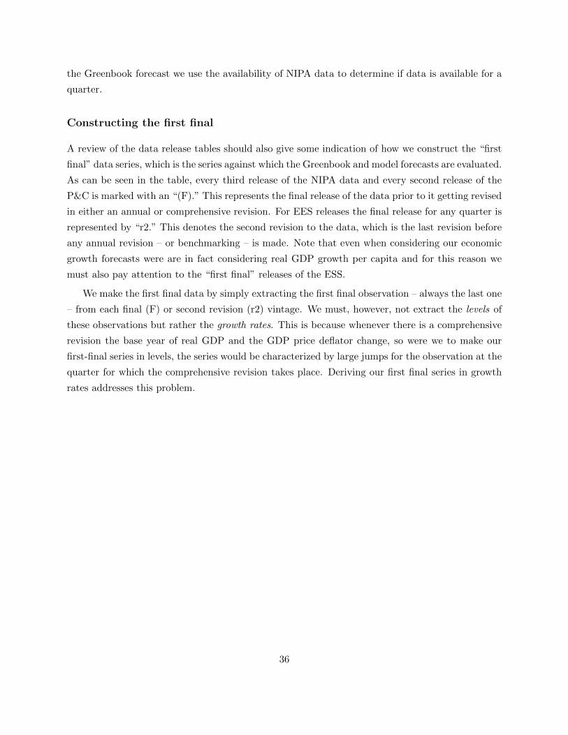
the Greenbook forecast we use the availability of NIPA data to determine if data is available for a

quarter.

Constructing the first final

A review of the data release tables should also give some indication of how we construct the “first

final” data series, which is the series against which the Greenbook and model forecasts are evaluated.

As can be seen in the table, every third release of the NIPA data and every second release of the

P&C is marked with an “(F).” This represents the final release of the data prior to it getting revised

in either an annual or comprehensive revision. For EES releases the final release for any quarter is

represented by “r2.” This denotes the second revision to the data, which is the last revision before

any annual revision – or benchmarking – is made. Note that even when considering our economic

growth forecasts were are in fact considering real GDP growth per capita and for this reason we

must also pay attention to the “first final” releases of the ESS.

We make the first final data by simply extracting the first final observation – always the last one

– from each final (F) or second revision (r2) vintage. We must, however, not extract the levels of

these observations but rather the growth rates. This is because whenever there is a comprehensive

revision the base year of real GDP and the GDP price deflator change, so were we to make our

first-final series in levels, the series would be characterized by large jumps for the observation at the

quarter for which the comprehensive revision takes place. Deriving our first final series in growth

rates addresses this problem.

36

F’c

ast

GB

GB

F’c

ast

Inte

rim

NIP

AIn

teri

mP

&C

Inte

rim

ES

SIn

teri

mE

SS

Nam

ecl

osed

hor

izon

rele

ase

sre

lease

sre

lease

s(m

thly

)re

lease

s(q

rtly

)

91:Q

3(F

):12/20/91

91:Q

3(F

):1/3/92

91:D

ec&

CPS

91:Q

4:1/10/92

91:Q

4(A

):1/29/92

Rev

isions:

1/10/92

Jan

.92∗

1/30

/92

92:Q

1-93

:Q4

91:Q

4(P

):2/28/92

91:Q

4(P

):2/5/92

92:Jan:2/7/92

91:Q

4(r1):

2/7/92

91:Q

4(F

)&

Ann.

92:Feb

:3/6/92

91:Q

4(r2):

3/6/92

Rev

isions:

3/10/92

Mar

.92

3/25

/92

92:Q

1-93

:Q4

91:Q

4(F

):3/26/92

–92:M

ar:

4/3/92

92:Q

1:4/3/92

92:Q

1(A

):4/28/92

92:A

pr:

5/8/92

92:Q

1(r1):

5/8/92

May

92∗

5/14

/92

92:Q

2-93

:Q4

92:Q

1(P

):5/29/92

92:Q

1(P

,F):

6/17/92

92:M

ay&

CES

92:Q

1(r2):

6/5/92

92:Q

1(F

):6/25/92

Rev

isions:

6/5/92

Ju

n.

926/

26/9

292

:Q2-

93:Q

492:Q

2(A

)&

Ann.

92:Q

2(P

)&

NIP

A92:Jun:7/2/92

92:Q

2:7/2/92

Rev

isions:

7/30/92

Rev

isions:

8/11/92

92:Jul:

8/7/92

92:Q

2(r1):

8/7/92

Au

g.92

8/13

/92

92:Q

3-93

:Q4

92:Q

2(P

):8/27/92

92:Q

2(F

):9/3/92

92:A

ug:9/4/92

92:Q

2(r2):

9/4/92

92:Q

2(F

):9/24/92

Sep

.92

9/30

/92

92:Q

3-94

:Q4

92:Q

3(A

):10/27/92

92:Q

3(P

):11/5/92

92:Sep

:10/2/92

92:Q

3:10/2/92

92:O

ct:11/6/92

92:Q

3(r1):

11/6/92

Nov

.92

11/1

2/92

92:Q

4-94

:Q4

92:Q

3(P

):11/25/92

92:Q

3(F

):12/3/92

92:N

ov:12/4/92

92:Q

3(r2):

12/4/92

Dec

.92

12/1

6/92

92:Q

4-94

:Q4

Tab

le5:

Gre

enb

ook

For

ecas

tsan

dN

IPA

,P

&C

.am

dE

mp

loym

ent

Sit

uat

ion

Rel

ease

Dat

es,

1992

.

37

F’c

ast

GB

GB

F’c

ast

Inte

rim

NIP

AIn

teri

mP

&C

Inte

rim

ES

SIn

teri

mE

SS

Nam

ecl

osed

hor

izon

rele

ase

sre

lease

sre

lease

s(m

thly

)re

lease

s(q

rtly

)

92:Q

3(F

):12/20/92

–92:D

ec&

CPS

92:Q

4:1/8/93

92:Q

4(A

):1/28/93

Rev

isions:

1/8/93

Jan

.93∗

1/29

/93

93:Q

1-94

:Q4

92:Q

4(P

):2/26/93

92:Q

4(P

):2/4/93

93:Jan&

CES

92:Q

4(r1):

2/5/93

92:Q

4(F

)&

Ann.

93:Feb

:3/5/93

92:Q

4(r2):

3/5/93

Rev

isions:

3/9/93

Mar

.93

3/17

/93

93:Q

1-94

:Q4

92:Q

4(F

):3/26/93

93:Q

1(P

):5/6/93

93:M

ar:

4/2/93

93:Q

1:4/2/93

93:Q

1(A

):4/29/93

93:A

pr:

5/7/93

93:Q

1(r1):

5/7/93

May

935/

14/9

393

:Q2-

94:Q

493:Q

1(P

):5/28/93

93:Q

1(F

):6/17/93

93:M

ay&

CES

93:Q

1(r2):

6/4/93

93:Q

1(F

):6/23/93

Rev

isions:

6/4/93

Ju

n.

936/

30/9

393

:Q2-

94:Q

493:Q

2(A

)&

Ann.

93:Q

2(P

)&

NIP

A93:Jun:7/2/93

93:Q

2:7/2/93

Rev

isions:

7/29/93

Rev

isions:

8/10/93

93:Jul:

8/6/93

93:Q

2(r1):

8/6/93

Au

g.93

8/11

/93

93:Q

3-94

:Q4

93:Q

2(P

):8/31/93

93:Q

2(F

):9/9/93

93:A

ug:9/3/93

93:Q

2(r2):

9/3/93

Sep

.93

9/15

/93

93:Q

3-95

:Q4

93:Q

2(F

):9/29/93

93:Q

3(P

):11/4/93

93:Sep

:10/8/93

93:Q

3:10/8/93

93:Q

3(A

):10/28/93

93:O

ct:11/5/93

93:Q

3(r1):

11/5/93

Nov

.93

11/1

0/93

93:Q

4-95

:Q4

93:Q

3(P

):12/1/93

93:Q

3(F

):12/8/93

93:N

ov:12/3/93

93:Q

3(r2):

12/3/93

Dec

.93

12/1

5/93

93:Q

4-95

:Q4

Tab

le6:

Gre

enb

ook

For

ecas

tsan

dN

IPA

,P

&C

.am

dE

mp

loym

ent

Sit

uat

ion

Rel

ease

Dat

es,

1993

.

38

F’c

ast

GB

GB

F’c

ast

Inte

rim

NIP

AIn

teri

mP

&C

Inte

rim

ES

SIn

teri

mE

SS

Nam

ecl

osed

hor

izon

rele

ase

sre

lease

sre

lease

s(m

thly

)re

lease

s(q

rtly

)

93:Q

3(F

):12/22/93

–93:D

ec&

CPS

93:Q

4:1/7/94

93:Q

4(A

):1/28/94

Rev

isions:

1/7/94

Jan

.94∗

1/31

/94

94:Q

1-95

:Q4

93:Q

4(P

):3/1/94

93:Q

4(P

):2/8/94

94:Jan:2/4/94

93:Q

4(r1):

2/4/94

93:Q

4(F

)&

Ann.

94:Feb

:3/4/94

93:Q

4(r2):

3/4/94

Rev

isions:

3/8/94

Mar

.94

3/16

/94

94:Q

1-95

:Q4

93:Q

4(F

):3/31/94

94:Q

1(P

):5/5/94

94:M

ar:

4/1/94

94:Q

1:4/1/94

94:Q

1(A

):4/28/94

94:A

pr:

5/6/94

94:Q

1(r1):

5/6/94

May

945/

13/9

494

:Q2-

95:Q

494:Q

1(P

):5/27/94

94:Q

1(F

):6/15/94

94:M

ay&

CES

94:Q

1(r2):

6/3/94

94:Q

1(F

):6/29/94

Rev

isions:

6/3/94

Ju

n.

946/

30/9

494

:Q2-

95:Q

494:Q

2(A

)&

Ann.

94:Q

2(P

)&

NIP

A94:Jun:7/8/94

94:Q

2:7/8/94

Rev

isions:

7/29/94

Rev

isions:

8/9/94

94:Jul:

8/5/94

94:Q

2(r1):

8/5/94

Au

g.94

8/12

/94

94:Q

3-95

:Q4

94:Q

2(P

):8/26/94

94:Q

2(F

):9/7/94

94:A

ug:9/2/94

94:Q

2(r2):

9/2/94

Sep

.94

9/21

/94

94:Q

3-96

:Q4

94:Q

2(F

):9/29/94

94:Q

3(P

):11/9/94

94:Sep

:10/7/94

94:Q

3:10/7/94

94:Q

3(A

):10/28/94

94:O

ct:11/4/94

94:Q

3(r1):

11/4/94

Nov

.94

11/9

/94

94:Q

4-96

:Q4

94:Q

3(P

):11/30/94

94:Q

3(F

):12/7/94

94:N

ov:12/2/94

94:Q

3(r2):

12/2/94

Dec

.94

12/1

4/94

94:Q

4-96

:Q4

Tab

le7:

Gre

enb

ook

For

ecas

tsan

dN

IPA

,P

&C

.am

dE

mp

loym

ent

Sit

uat

ion

Rel

ease

Dat

es,

1994

.

39

F’c

ast

GB

GB

F’c

ast

Inte

rim

NIP

AIn

teri

mP

&C

Inte

rim

ES

SIn

teri

mE

SS

Nam

ecl

osed

hor

izon

rele

ase

sre

lease

sre

lease

s(m

thly

)re

lease

s(q

rtly

)

94:Q

3(F

):12/22/94

–94:D

ec&

CPS

94:Q

4:1/6/95

Rev

isions:

1/6/95

Jan

.95†

1/25

/95

95:Q

1-96

:Q4

94:Q

4(A

):1/27/95

94:Q

4(P

):2/7/95

95:Jan:2/3/95

94:Q

4(r1):

2/3/95

94:Q

4(P

):3/1/95

94:Q

4(F

)&

Ann.

95:Feb

:3/10/95

94:Q

4(r2):

3/10/95

Rev

isions:

3/8/95

Mar

.95

3/22

/95

95:Q

1-96

:Q4

94:Q

4(F

):3/31/95

95:Q

1(P

):5/9/95

95:M

ar:

4/7/95

95:Q

1:4/7/95

95:Q

1(A

):4/28/95

95:A

pr:

5/5/95

95:Q

1(r1):

5/5/95

May

955/

17/9

595

:Q2-

96:Q

495:Q

1(P

):5/31/95

–95:M

ay&

CES

95:Q

1(r2):

6/2/95

Rev

isions:

6/2/95

Ju

n.

956/

20/9

595

:Q2-

96:Q

495:Q

1(F

):6/30/95

95:Q

1(F

):6/21/95

95:Jun:7/7/95

95:Q

2:7/7/95

95:Q

2(A

)&

Ann.

95:Q

2(P

)&

NIP

A95:Jul:

8/4/95

95:Q

2(r1):

8/4/95

Rev

isions:

7/28/95

Rev

isions:

8/8/95

Au

g.95

8/16

/95

95:Q

3-96

:Q4

95:Q

2(P

):8/30/95

95:Q

2(F

):9/7/95

95:A

ug:9/1/95

95:Q

2(r2):

9/1/95

Sep

.95

9/20

/95

95:Q

3-97

:Q4

95:Q

2(F

):9/29/95

95:Q

3(P

):11/7/95

95:Sep

:10/6/95

95:Q

3:10/6/95

95:Q

3(A

):10/27/95

95:O

ct:11/3/95

95:Q

3(r1):

11/3/95

Nov

.95

11/8

/95

95:Q

4-97

:Q4

Shutd

own

Shutd

own

95:N

ov:12/8/95

95:Q

3(r2):

12/8/95

Dec

.95

12/1

4/95

95:Q

4-97

:Q4

Tab

le8:

Gre

enb

ook

For

ecas

tsan

dN

IPA

,P

&C

.am

dE

mp

loym

ent

Sit

uat

ion

Rel

ease

Dat

es,

1995

.

40

F’c

ast

GB

GB

F’c

ast

Inte

rim

NIP

AIn

teri

mP

&C

Inte

rim

ES

SIn

teri

mE

SS

Nam

ecl

osed

hor

izon

rele

ase

sre

lease

sre

lease

s(m

thly

)re

lease

s(q

rtly

)

95:Q

3(P

,F)andComp.

–95:D

ec&

CPS

95:Q

4:1/19/96

Rev

isions:

1/19/96

Rev

isions:

1/19/96

Jan

.96∗

1/26

/96

96:Q

1-97

:Q4

95:Q

4(A

,P):

2/23/96

95:Q

3(F

):2/8/96

96:Jan:2/2/96

95:Q

4(r1):

2/2/96

95:Q

4(P

)&

Ann.

96:Feb

:3/8/96

95:Q

4(r2):

3/8/96

Rev

isions:

3/6/96

Mar

.96

3/21

/96

96:Q

1-97

:Q4

95:Q

4(F

):4/2/96

95:Q

4(F

):4/10/96

96:M

ar:

4/5/96

96:Q

1:4/5/96

96:Q

1(A

):5/2/96

96:Q

1(P

):5/16/96

96:A

pr:

5/3/96

96:Q

1(r1):

5/3/96

May

965/

16/9

696

:Q2-

97:Q

496:Q

1(P

):5/30/96

96:Q

1(F

):6/18/96

96:M

ay&

CES

96:Q

1(r2):

6/7/96

Rev

isions:

6/7/96

Ju

n.

966/

26/9

696

:Q2-

97:Q

496:Q

1(F

):6/28/96

96:Q

2(P

)&

NIP

A96:Jun:7/5/96

96:Q

2:7/5/96

96:Q

2(A

)&

Ann.

Rev

isions:

8/14/96

96:Jul:

8/2/96

96:Q

2(r1):

8/2/96

Rev

isions:

8/1/96

Au

g.96

8/15

/96

96:Q

3-97

:Q4

96:Q

2(P

):8/29/96

96:Q

2(F

):9/10/96

96:A

ug:9/6/96

96:Q

2(r2):

9/6/96

Sep

.96

9/18

/96

96:Q

3-98

:Q4

96:Q

2(F

):9/27/96

–96:Sep

:10/4/96

96:Q

3:10/4/96

96:Q

3(A

):10/30/96

Nov

.96∗

11/6

/96

96:Q

4-98

:Q4

96:Q

3(P

):11/27/96

96:Q

3(P

):11/7/96

96:O

ct:11/1/96

96:Q

3(r1):

11/1/96

96:Q

3(F

):12/5/96

96:N

ov:12/6/96

96:Q

3(r2):

12/6/96

Dec

.96

12/1

2/96

96:Q

4-98

:Q4

Tab

le9:

Gre

enb

ook

For

ecas

tsan

dN

IPA

,P

&C

.am

dE

mp

loym

ent

Sit

uat

ion

Rel

ease

Dat

es,

1996

.

41

F’c

ast

GB

GB

F’c

ast

Inte

rim

NIP

AIn

teri

mP

&C

Inte

rim

ESS

Inte

rim

ESS

Nam

ecl

osed

hor

izon

rele

ase

sre

lease

sre

lease

s(m

thly

)re

lease

s(q

rtly

)

96:Q

3(F

):12/20/96

–96:D

ec&

CPS

96:Q

4:1/10/97

Rev

isions:

1/10/97

Jan

.97†

1/29

/97

97:Q

1-98

:Q4

96:Q

4(A

):1/31/97

96:Q

4(P

):2/11/97

97:Jan:2/7/97

96:Q

4(r1):

2/7/97

96:Q

4(P

):2/28/97

96:Q

4(F

)&

Ann.

97:Feb

:3/7/97

96:Q

4(r2):

3/7/97

Rev

isions:

3/11/97

Mar

.97

3/19

/97

97:Q

1-98

:Q4

96:Q

4(F

):3/28/97

97:Q

1(P

):5/7/97

97:M

ar:

4/4/97

97:Q

1:4/4/97

97:Q

1(A

):4/30/97

97:A

pr:

5/2/97

97:Q

1(r1):

5/2/97

97:Q

1(A

,Err):

5/7/97

May

975/

15/9

797

:Q2-

98:Q

497:Q

1(P

):5/30/97

97:Q

1(F

):6/18/97

97:M

ay&

CES

97:Q

1(r2):

6/6/97

Rev

isions:

6/6/97

Ju

n.

976/

25/9

797

:Q2-

98:Q

497:Q

1(F

):6/27/97

97:Q

2(P

)&

NIP

A97:Jun:7/3/97

97:Q

2:7/3/97

97:Q

2(A

)&

Ann.

Rev

isions:

8/12/97

97:Jul:

8/1/97

97:Q

2(r1):

8/1/97

Rev

isions:

7/31/97

Au

g.97

8/14

/97

97:Q

3-98

:Q4

97:Q

2(P

):8/28/97

97:Q

2(F

):9/9/97

97:A

ug:9/5/97

97:Q

2(r2):

9/5/97

Sep

.97

9/24

/97

97:Q

3-99

:Q4

97:Q

2(F

):9/26/97

–97:Sep

:10/3/97

97:Q

3:10/3/97

97:Q

3(A

):10/31/97

Nov

.97∗

11/6

/97

97:Q

4-99

:Q4

97:Q

3(P

):11/26/97

97:Q

3(P

):11/13/97

97:O

ct:11/7/97

97:Q

3(r1):

11/7/97

97:Q

3(F

):12/4/97

97:N

ov:12/5/97

97:Q

3(r2):

12/5/97

Dec

.97

12/1

1/97

97:Q

4-99

:Q4

Tab

le10

:G

reen

book

For

ecas

tsan

dN

IPA

,P

&C

.am

dE

mp

loym

ent

Sit

uat

ion

Rel

ease

Dat

es,

1997

.

42

F’c

ast

GB

GB

F’c

ast

Inte

rim

NIP

AIn

teri

mP

&C

Inte

rim

ES

SIn

teri

mE

SS

Nam

ecl

osed

hor

izon

rele

ase

sre

lease

sre

lease

s(m

thly

)re

lease

s(q

rtly

)

97:Q

3(F

):12/23/97

–97:D

ec&

CPS

97:Q

4:1/9/98

Rev

isions:

1/9/98

Jan

.98†

1/28

/98

98:Q

1-99

:Q4

97:Q

4(A

):1/30/98

97:Q

4(P

):2/10/98

98:Jan:2/6/98

97:Q

4(r1):

2/6/98

97:Q

4(P

):2/27/98

97:Q

4(F

)&

Ann.

98:Feb

:3/6/98

97:Q

4(r2):

3/6/98

Rev

isions:

3/10/98

Mar

.98

3/19

/98

98:Q

1-99

:Q4

97:Q

4(F

):3/26/98

98:Q

1(P

):5/07/98

98:M

ar:

4/3/98

98:Q

1:4/3/98

98:Q

1(A

):4/30/98

98:A

pr:

5/8/98

98:Q

1(r1):

5/8/98

May

985/

14/9

898

:Q2-

99:Q

498:Q

1(P

):5/28/98

98:Q

1(F

):6/4/98

98:M

ay&

CES

98:Q

1(r2):

6/5/98

Rev

isions:

6/5/98

Ju

n.

986/

24/9

898

:Q2-

99:Q

498:Q

1(F

):6/25/98

98:Q

2(P

)&

NIP

A98:Jun:7/2/98

98:Q

2:7/2/98

98:Q

2(A

)&

Ann.

Rev

isions:

8/8/98

98:Jul:

8/7/98

98:Q

2(r1):

8/7/98

Rev

isions:

7/31/98

Au

g.98

8/13

/98

98:Q

3-99

:Q4

98:Q

2(P

):8/27/98

98:Q

2(F

):9/3/98

98:A

ug:9/4/98

98:Q

2(r2):

9/4/98

Sep

.98

9/23

/98

98:Q

3-00

:Q4

98:Q

2(F

):9/24/98

98:Q

3(P

):11/10/98

98:Sep

:10/2/98

98:Q

3:10/2/98

98:Q

3(A

):10/30/98

98:O

ct:11/5/98

98:Q

3(r1):

11/5/98

Nov

.98

11/1

3/98

98:Q

4-00

:Q4

98:Q

3(P

):11/24/98

98:Q

3(F

):12/3/98

98:N

ov:12/4/98

98:Q

3(r2):

12/4/98

Dec

.98

12/1

6/98

98:Q

4-00

:Q4

Tab

le11

:G

reen

book

For

ecas

tsan

dN

IPA

,P

&C

.am

dE

mp

loym

ent

Sit

uat

ion

Rel

ease

Dat

es,

1998

.

43

F’c

ast

GB

GB

F’c

ast

Inte

rim

NIP

AIn

teri

mP

&C

Inte

rim

ESS

Inte

rim

ESS

Nam

ecl

osed

hor

izon

rele

ase

sre

lease

sre

lease

s(m

thly

)re

lease

s(q

rtly

)

98:Q

3(F

):12/23/98

–98:D

ec&

CPS

98:Q

4:1/8/99

Rev

isions:

1/8/99

Jan

.99†

1/10

/99

99:Q

1-00

:Q4

98:Q

4(A

):1/29/99

98:Q

4(P

):2/9/99

99:Jan:2/5/99

98:Q

4(r1):

2/5/99

98:Q

4(P

):2/26/99

98:Q

4(F

)&

Ann.

99:Feb

:3/5/99

98:Q

4(r2):

3/5/99

Rev

isions:

3/9/99

Mar

.99

3/10

/99

99:Q

1-00

:Q4

98:Q

4(F

):3/31/99

99:Q

1(P

):5/11/99

99:M

ar:

4/2/99

99:Q

1:4/2/99

99:Q

1(A

):4/30/99

99:A

pr:

5/7/99

99:Q

1(r1):

5/7/99

May

995/

10/9

999

:Q2-

00:Q

499:Q

1(P

):5/27/99

99:Q

1(F

):6/8/99

99:M

ay&

CES

99:Q

1(r2):

6/4/99

Rev

isions:

6/4/99

Ju

n.

996/

10/9

999

:Q2-

00:Q

499:Q

1(F

):6/25/99

99:Q

2(P

):8/5/99

99:Jun:7/2/99

99:Q

2:7/2/99

99:Q

2(A

):7/29/99

99:Jul:

8/6/99

99:Q

2(r1):

8/6/99

Au

g.99

8/10

/99

99:Q

3-00

:Q4

99:Q

2(P

):8/26/99

99:Q

2(F

):9/2/99

99:A

ug:9/3/99

99:Q

2(r2):

9/3/99

Sep

.99

9/10

/99

99:Q

3-01

:Q4

99:Q

2(F

):9/30/99

–99:Sep

:10/8/99

99:Q

3:10/8/99

99:Q

3(A

)&

Comp.

99:O

ct:11/5/99

99:Q

3(r1):

11/5/99

Rev

isions:

10/29/99

Nov

.99∗

11/1

0/99

99:Q

4-01

:Q4

99:Q

3(P

):11/24/99

99:Q

3(P

):11/12/99

99:N

ov:12/3/99

99:Q

3(r2):

12/3/99

99:Q

3(F

):12/7/99

Dec

.99

12/1

0/99

99:Q

4-01

:Q4

Tab

le12

:G

reen

book

For

ecas

tsan

dN

IPA

,P

&C

.am

dE

mp

loym

ent

Sit

uat

ion

Rel

ease

Dat

es,

1999

.

44

F’c

ast

GB

GB

F’c

ast

Inte

rim

NIP

AIn

teri

mP

&C

Inte

rim

ES

SIn

teri

mE

SS

Nam

ecl

osed

hor

izon

rele

ase

sre

lease

sre

lease

s(m

thly

)re

lease

s(q

rtly

)

99:Q

3(F

):12/22/99

–99:D

ec&

CPS

99:Q

4:1/7/00

Rev

isions:

1/7/00

Jan

.00†

1/27

/00

00:Q

1-01

:Q4

99:Q

4(A

):1/28/00

99:Q

4(P

):2/8/00

00:Jan:2/4/00

99:Q

4(r1):

2/4/00

99:Q

4(P

):2/25/00

99:Q

4(F

)&

Ann.

00:Feb

:3/3/00

99:Q

4(r2):

3/3/00

Rev

isions:

3/7/00

Mar

.00

3/15

/00

00:Q

1-01

:Q4

99:Q

4(F

):3/30/00

00:Q

1(P

):5/4/00

00:M

ar:

4/7/00

00:Q

1:4/7/00

99:Q

4(F

,r):

4/3/00

00:A

pr:

5/5/00

00:Q

1(r1):

5/5/00

00:Q

1(A

):4/27/00

May

005/

11/0

000

:Q2-

01:Q

400:Q

1(P

):5/25/00

00:Q

1(F

):6/6/00

00:M

ay&

CES

00:Q

1(r2):

6/2/00

Rev

isions:

6/2/00

Ju

n.

006/

21/0

000

:Q2-

01:Q

400:Q

1(F

):6/29/00

00:Q

2(P

)&

NIP

A00:Jun:7/7/00

00:Q

2:7/7/00

00:Q

2(A

)&

Ann.

Rev

isions:

8/8/00

00:Jul:

8/4/00

00:Q

2(r1):

8/4/00

Rev

isions:

7/28/00

Au

g.00

8/16

/00

00:Q

3-01

:Q4

00:Q

2(P

):8/25/00

00:Q

2(F

):9/6/00

00:A

ug:9/1/00

00:Q

2(r2):

9/1/00

Sep

.00

9/27

/00

00:Q

3-02

:Q4

00:Q

2(F

):9/28/00

00:Q

3(P

):11/2/00

00:Sep

:10/6/00

00:Q

3:10/6/00

00:Q

3(A

):10/27/00

00:O

ct:11/3/00

00:Q

3(r1):

11/3/00

Nov

.00

11/8

/00

00:Q

4-02

:Q4

00:Q

3(P

):11/29/00

00:Q

3(F

):12/6/00

00:N

ov:12/8/00

00:Q

3(r2):

12/8/00

Dec

.00

12/1

3/00

00:Q

4-02

:Q4

Tab

le13

:G

reen

book

For

ecas

tsan

dN

IPA

,P

&C

.am

dE

mp

loym

ent

Sit

uat

ion

Rel

ease

Dat

es,

2000

.

45

F’c

ast

GB

GB

F’c

ast

Inte

rim

NIP

AIn

teri

mP

&C

Inte

rim

ES

SIn

teri

mE

SS

Nam

ecl

osed

hor

izon

rele

ase

sre

lease

sre

lease

s(m

thly

)re

lease

s(q

rtly

)

00:Q

3(F

):12/21/00

–00:D

ec&

CPS

00:Q

4:1/5/01

Rev

isions:

1/5/01

Jan

.01†

1/25

/01

01:Q

1-02

:Q4

00:Q

4(A

):1/31/01

00:Q

4(P

):2/7/01

01:Jan:2/2/01

00:Q

4(r1):

2/2/01

00:Q

4(P

):2/28/01

00:Q

4(F

)&

Ann.

01:Feb

:3/9/01

00:Q

4(r2):

3/9/01

Rev

isions:

3/6/01

Mar

.01

3/14

/01

01:Q

1-02

:Q4

00:Q

4(F

):3/29/01

01:Q

1(P

):5/8/01

01:M

ar:

4/6/01

01:Q

1:4/6/01

01:Q

1(A

):4/27/01

01:A

pr:

5/4/01

01:Q

1(r1):

5/4/01

May

015/

9/01

01:Q

2-02

:Q4

01:Q

1(P

):5/25/01

01:Q

1(F

):6/5/01

01:M

ay&

CES

01:Q

1(r2):

6/1/01

Rev

isions:

6/1/01

Ju

n.

016/

20/0

101

:Q2-

02:Q

401:Q

1(F

):6/29/01

01:Q

2(P

)&

NIP

A01:Jun:7/6/01

01:Q

2:7/6/01

01:Q

2(A

)&

Ann.

Rev

isions:

8/7/01

01:Jul:

8/3/01

01:Q

2(r1):

8/3/01

Rev

isions:

7/27/01

Au

g.01

8/15

/01

01:Q

3-02

:Q4

01:Q

2(P

):8/29/01

01:Q

2(F

):9/5/01

01:A

ug:9/7/01

01:Q

2(r2):

9/7/01

Sep

.01

9/26

/01

01:Q

3-03

:Q4

01:Q

2(F

):9/28/01

–01:Sep

:10/5/01

01:Q

3:10/5/01

01:Q

3(A

):10/31/01

Oct

.01∗

10/3

1/01

01:Q

4-03

:Q4

01:Q

3(P

):11/30/01

01:Q

3(P

):11/7/01

01:O

ct:11/2/01

01:Q

3(r1):

11/2/01

Dec

.01

12/5

/01

01:Q

4-03

:Q4

Tab

le14

:G

reen

book

For

ecas

tsan

dN

IPA

,P

&C

.am

dE

mp

loym

ent

Sit

uat

ion

Rel

ease

Dat

es,

2001

.

46

F’c

ast

GB

GB

F’c

ast

Inte

rim

NIP

AIn

teri

mP

&C

Inte

rim

ES

SIn

teri

mE

SS

Nam

ecl

osed

hor

izon

rele

ase

sre

lease

sre

lease

s(m

thly

)re

lease

s(q

rtly

)

01:Q

3(F

):12/21/01

01:Q

3(F

):12/6/01

01:N

ov:12/7/01

01:Q

3(r2):

12/7/01

01:D

ec&

CPS

01:Q

4:1/4/02

Rev

isions:

1/4/05

Jan

.02†

1/23

/02

02:Q

1-03

:Q4

01:Q

4(A

):1/30/02

01:Q

4(P

):2/6/02

02:Jan:2/1/01

01:Q

4(r1):

2/1/02

01:Q

4(P

):2/28/02

01:Q

4(F

)&

Ann.

02:Feb

:3/8/02

01:Q

4(r2):

3/8/02

Rev

isions:

3/7/02

Mar

.02

3/13

/02

02:Q

1-03

:Q4

01:Q

4(F

):3/28/02

–02:M

ar:

4/5/02

02:Q

1:4/5/02

02:Q

1(A

):4/26/02

May

02∗

5/1/

0202

:Q2-

03:Q

402:Q

1(P

):5/24/02

02:Q

1(P

):5/7/02

02:A

pr:

5/3/02

02:Q

1(r1):

5/3/02

02:Q

1(F

):5/31/02

02:M

ay&

CES

02:Q

1(r2):

6/7/02

Rev

isions:

6/7/02

Ju

n.

026/

19/0

202

:Q2-

03:Q

402:Q

1(F

):6/27/02

–02:Jun:7/5/02

02:Q

2:7/5/02

02:Q

2(A

)&

Ann.

02:Jul:

8/2/02

02:Q

2(r1):

8/2/02

Rev

isions:

7/31/02

Au

g.02∗

8/7/

0202

:Q3-

03:Q

402:Q

2(P

):8/29/02

02:Q

2(P

)&

NIP

A02:A

ug:9/6/02

02:Q

2(r2):

9/6/02

Rev

isions:

8/9/02

02:Q

2(F

):9/5/02

Sep

.02

9/18

/02

02:Q

3-04

:Q4

02:Q

2(F

):9/27/02

–02:Sep

:10/4/02

02:Q

3:10/4/02

Oct

.02†

10/3

0/02

02:Q

4-04

:Q4

02:Q

3(A

):10/31/02

02:Q

3(P

):11/7/02

02:O

ct:11/1/02

02:Q

3(r1):

11/1/02

02:Q

3(P

):11/26/02

02:Q

3(F

):12/4/02

Dec

.02

12/4

/02

02:Q

4-04

:Q4

Tab

le15

:G

reen

book

For

ecas

tsan

dN

IPA

,P

&C

.am

dE

mp

loym

ent

Sit

uat

ion

Rel

ease

Dat

es,

2002

.

47

F’c

ast

GB

GB

F’c

ast

Inte

rim

NIP

AIn

teri

mP

&C

Inte

rim

ES

SIn

teri

mE

SS

Nam

ecl

osed

hor

izon

rele

ase

sre

lease

sre

lease

s(m

thly

)re

lease

s(q

rtly

)

02:Q

3(F

):12/20/02

–02:N

ov:12/6/02

02:Q

3(r2):

12/6/02

02:D

ec&

CPS

02:Q

4:1/10/03

Rev

isions:

1/10/03

Jan

.03†

1/22

/03

03:Q

1-04

:Q4

02:Q

4(A

):1/30/03

02:Q

4(P

):2/6/03

03:Jan:2/7/03

02:Q

4(r1):

2/7/03

02:Q

4(P

):2/28/03

02:Q

4(F

)&

Ann.

03:Feb

:3/7/03

02:Q

4(r2):

3/7/03

Rev

isions:

3/6/03

Mar

.03

3/12

/03

03:Q

1-04

:Q4

02:Q

4(F

):3/27/03

–03:M

ar:

4/4/03

03:Q

1:4/4/03

03:Q

1(A

):4/25/03

Ap

r.03∗

4/30

/03

03:Q

2-04

:Q4

03:Q

1(P

):5/29/03

03:Q

1(P

):5/1/03

03:A

pr:

5/2/03

03:Q

1(r1):

5/2/03

03:Q

1(F

):6/4/03

03:M

ay&

CES

03:Q

1(r2):

6/6/03

Rev

isions:

6/6/03

Ju

n.

036/

18/0

303

:Q2-

04:Q

403:Q

1(F

):6/26/03

–03:Jun:7/3/03

03:Q

2:7/3/03

03:Q

2(A

):7/31/03

03:Jul:

8/1/03

03:Q

2(r1):

8/1/03

Au

g.03∗

8/6/

0303

:Q3-

04:Q

403:Q

2(P

):8/28/03

03:Q

2(P

):8/7/03

03:A

ug:9/5/03

03:Q

2(r2):

9/5/03

03:Q

2(F

):9/4/03

Sep

.03

9/10

/03

03:Q

3-05

:Q4

03:Q

2(F

):9/26/03

–03:Sep

:10/3/03

03:Q

3:10/3/03

Oct

.03†

10/2

2/03

03:Q

4-05

:Q4

03:Q

3(A

):10/30/03

03:Q

3(P

):11/6/03

03:O

ct:11/7/03

03:Q

3(r1):

11/7/03

03:Q

3(P

):11/25/03

03:Q

3(F

):12/3/03

Dec

.03

12/3

/03

03:Q

4-05

:Q4

Tab

le16

:G

reen

book

For

ecas

tsan

dN

IPA

,P

&C

.am

dE

mp

loym

ent

Sit

uat

ion

Rel

ease

Dat

es,

2003

.

48

F’c

ast

GB

GB

F’c

ast

Inte

rim

NIP

AIn

teri

mP

&C

Inte

rim

ESS

Inte

rim

ESS

Nam

ecl

osed

hor

izon

rele

ase

sre

lease

sre

lease

s(m

thly

)re

lease

s(q

rtly

)

Comp.Rev

.:12/10/03

–03:N

ov:12/5/03

03:Q

3(r2):

12/5/03

03:Q

3(F

):12/23/03

03:D

ec&

CPS

03:Q

4:1/9/04

Rev

isions:

1/9/04

Jan

.04†

1/21

/04

04:Q

1-0

5:Q

403:Q

4(A

):1/30/04

03:Q

4(P

):2/5/04

04:Jan&

CES

03:Q

4(r1):

2/6/04

03:Q

4(P

):2/27/04

03:Q

4(F

)&

Ann.

Rev

isions:

2/6/06

03:Q

4(r2):

3/5/04

Rev

isions:

3/4/04

04:Feb

:3/5/04

Mar

.04

3/10

/04

04:Q

1-0

5:Q

407:Q

4(F

):3/25/04

–04:M

ar:

4/2/04

04:Q

1:4/2/04

Ap

r.04

4/28

/04

04:Q

2-0

5:Q

404:Q

1(A

):4/29/04

04:Q

1(P

):5/6/04

04:A

pr:

5/7/04

04:Q

1(r1):

5/7/04

04:Q

1(P

):5/27/04

04:Q

1(F

):6/3/04

04:M

ay:6/4/04

04:Q

1(r2):

6/4/04

Ju

n.

046/

23/0

404

:Q2-0

5:Q

404:Q

1(F

):6/25/04

–04:Jun:7/2/04

04:Q

2:7/2/04

04:Q

2(A

)&

Ann.

Rev

ision:7/30/04

Au

g.04∗

8/4/

0404

:Q3-0

5:Q

404:Q

2(P

):8/27/04

04:Q

2(P

)&

NIP

A04:Jul:

8/6/04

04:Q

2(r1):

8/6/04

Rev

ision:8/10/04

04:A

ug:9/3/04

04:Q

2(r2):

9/3/04

04:Q

2(F

):9/2/04

Sep

.04

9/15

/04

04:Q

3-0

6:Q

404:Q

2(F

):9/29/04

04:Q

2(E

rr.):10/13/04

04:Sep

:10/8/04

04:Q

3:10/8/04

04:Q

3(A

):10/29/04

Nov

.04

11/3

/04

04:Q

4-0

6:Q

404:Q

3(P

):11/30/04

04:Q

3(P

):11/4/04

04:O

ct:11/5/04

04:Q

3(r1):

11/5/04

04:Q

3(F

):12/7/04

04:N

ov:12/3/04

04:Q

3(r2):

12/3/04

Dec

.04

12/8

/04

04:Q

4-0

6:Q

4

Tab

le17

:G

reen

book

For

ecas

tsan

dN

IPA

,P

&C

.am

dE

mp

loym

ent

Sit

uat

ion

Rel

ease

Dat

es,

2004

.

49

F’c

ast

Blu

eCh

ipB

CF

’cas

tIn

teri

mN

IPA

Inte

rim

P&

CIn

teri

mE

ES

Inte

rim

EE

SN

ame

rele

ased

hor

izon

rele

ase

sre

lease

sre

lease

s(m

thly

)re

lease

s(q

rtly

)

91:Q

3(F

):12/20/91

91:Q

3(F

):1/3/92

91:N

ov:12/6/91

91:Q

3(r2):

12/6/91

Jan

.92†

1/10

/92

91:Q

4-93

:Q4

91:D

ec&

CPS

91:Q

4:1/10/92

Rev

isions:

1/10/92

91:Q

4(A

):1/29/92

96:Q

4(P

):2/05/92

92:Jan:2/7/92

91:Q

4(r1):

2/7/92

Feb

.92

2/10

/92

92:Q

1-93

:Q4

91:Q

4(P

):2/28/92

92:Feb

:3/6/92

91:Q

4(r2):

3/6/92

Mar

.92

3/10

/92

92:Q

1-93

:Q4

96:Q

4(P

):3/10/92

91:Q

4(F

):3/26/92

92:M

ar:

4/3/92

92:Q

1:4/3/92

Ap

r.92†

4/10

/92

92:Q

1-93

:Q4

92:Q

1(A

):4/28/92

–92:A

pr:

5/8/92

92:Q

1(r1):

5/8/92

May

92∗

5/10

/92

92:Q

2-93

:Q4

92:Q

1(P

):5/29/92

–92:M

ay&

CES

92:Q

1(r2):

6/5/92

92:Q

1(F

):6/25/92

Rev

isions:

6/5/92

Ju

n.

92∗

6/10

/92

92:Q

2-93

:Q4

92:Q

1(F

):6/25/92

92:Q

1(P

,F):

6/17/92

92:Jun:7/2/92

92:Q

2:7/2/92

Ju

l.92†

7/10

/92

92:Q

2-93

:Q4

92:Q

2(A

)&

Ann.

–92:Jul:

8/7/92

92:Q

2(r1):

8/7/92

Rev

isions:

7/30/92

Au

g.92∗

8/10

/92

92:Q

3-93

:Q4

92:Q

2(P

):8/27/92

92:Q

2(P

):8/11/92

92:A

ug:9/4/92

92:Q

2(r2):

9/4/92

92:Q

2(F

):9/3/92

Sep

.92

9/10

/92

92:Q

3-93

:Q4

92:Q

2(F

):9/24/92

–92:Sep

:10/2/92

92:Q

3:10/2/92

Oct

.92†

10/1

0/92

92:Q

3-93

:Q4

92:Q

3(A

):10/27/92

92:Q

3(P

):11/05/92

92:O

ct:11/6/92

92:Q

3(r1):

11/6/92

Nov

.92

11/1

0/92

92:Q

4-93

:Q4

92:Q

3(P

):11/25/92

92:Q

3(F

):12/3/92

92:N

ov:12/4/92

92:Q

3(r2):

12/4/92

Dec

.92

12/1

0/92

92:Q

4-93

:Q4

Tab

le18:

Blu

eC

hip

For

ecas

tsan

dN

IPA

,P

&C

.am

dE

mp

loym

ent

Sit

uat

ion

Rel

ease

Dat

es,

1992

.

50

F’c

ast

Blu

eCh

ipB

CF

’cas

tIn

teri

mN

IPA

Inte

rim

P&

CIn

teri

mE

ES

Inte

rim

EE

SN

ame

rele

ased

hor

izon

rele

ase

sre

lease

sre

lease

s(m

thly

)re

lease

s(q

rtly

)

92:Q

3(F

):12/22/92

–92:D

ec&

CPS

92:Q

4:1/8/93

Rev

isions:

1/8/93

Jan

.93†

1/10

/93

92:Q

4-94

:Q4

92:Q

4(A

):1/28/93

92:Q

4(P

):2/4/93

93:Jan:2/5/93

92:Q

4(r1):

2/5/93

Feb

.93

2/10

/93

93:Q

1-94

:Q4

92:Q

4(P

):2/26/93

92:Q

4(F

)&

Ann.

93:Feb

:3/5/93

92:Q

4(r2):

3/5/93

Rev

isions:

3/9/93

Mar

.93

3/10

/93

93:Q

1-94

:Q4

92:Q

4(F

):3/26/93

–93:M

ar:

4/2/93

93:Q

1:4/2/93

Ap

r.93†

4/10

/93

93:Q

1-94

:Q4

93:Q

1(A

):4/29/93

93:Q

1(P

):5/6/93

93:A

pr:

5/7/93

93:Q

1(r1):

5/7/93

May

935/

10/9

393

:Q2-

94:Q

493:Q

1(P

):5/28/93

–93:M

ay&

CES

93:Q

1(r2):

6/4/93

93:Q

1(F

):6/23/93

Rev

isions:

6/4/93

Ju

n.

936/

10/9

393

:Q2-

94:Q

493:Q

1(F

):6/23/93

93:Q

1(F

):6/17/93

93:Jun:7/2/93

93:Q

2:7/2/93

Ju

l.93†

7/10

/93

93:Q

2-94

:Q4

93:Q

2(A

)7/29/93

–93:Jul:

8/6/93

93:Q

2(r1):

8/6/93

Au

g.93

8/10

/93

93:Q

3-94

:Q4

93:Q

2(P

):8/10/93

93:Q

2(P

)&

Ann.

93:Q

2(F

):9/9/93

93:A

ug:9/3/93

93:Q

2(r2):

9/3/93

Rev

isions:

8/31/93

Sep

.93

9/10

/93

93:Q

3-94

:Q4

93:Q

2(F

):9/29/93

–93:Sep

:10/8/93

93:Q

3:10/8/93

Oct

.93†

10/1

0/93

93:Q

3-94

:Q4

93:Q

3(A

):10/28/93

93:Q

3(P

):11/4/93

93:O

ct:11/5/93

93:Q

3(r1):

11/5/93

Nov

.93

11/1

0/93

93:Q

4-94

:Q4

93:Q

3(P

):12/1/93

93:Q

3(F

):12/8/93

93:N

ov:12/3/93

93:Q

3(r2):

12/3/93

Dec

.93

12/1

0/93

93:Q

4-94

:Q4

Tab

le19:

Blu

eC

hip

For

ecas

tsan

dN

IPA

,P

&C

.am

dE

mp

loym

ent

Sit

uat

ion

Rel

ease

Dat

es,

1993

.

51

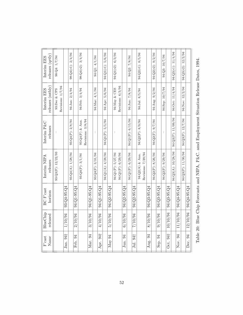
F’c

ast

Blu

eCh

ipB

CF

’cas

tIn

teri

mN

IPA

Inte

rim

P&

CIn

teri

mE

ES

Inte

rim

EE

SN

ame

rele

ased

hor

izon

rele

ase

sre

lease

sre

lease

s(m

thly

)re

lease

s(q

rtly

)

93:Q

3(F

):12/22/93

–93:D

ec&

CPS

98:Q

4:1/7/94

Rev

isions:

1/7/94

Jan

.94†

1/10

/94

93:Q

4-95

:Q4

93:Q

4(A

):1/28/94

93:Q

4(P

):2/8/94

94:Jan:2/4/94

98:Q

4(r1):

2/4/94

Feb

.94

2/10

/94

94:Q

1-95

:Q4

93:Q

4(P

):3/1/94

93:Q

4(F

)&

Ann.

94:Feb

:3/4/94

98:Q

4(r2):

3/4/94

Rev

isions:

3/8/94

Mar

.94

3/10

/94

94:Q

1-95

:Q4

93:Q

4(F

):3/31/94

–94:M

ar:

4/1/94

94:Q

1:4/1/94

Ap

r.94†

4/10

/94

94:Q

1-95

:Q4

94:Q

1(A

):4/28/94

94:Q

1(P

):5/5/94

94:A

pr:

5/6/94

94:Q

1(r1):

5/6/94

May

945/

10/9

494

:Q2-

95:Q

494:Q

1(P

):5/27/94

–94:M

ay&

CES

94:Q

1(r2):

6/3/94

94:Q

1(F

):6/29/94

Rev

isions:

6/3/94

Ju

n.

946/

10/9

494

:Q2-

95:Q

494:Q

1(F

):6/29/94

94:Q

1(F

):6/15/94

94:Jun:7/8/94

94:Q

2:7/8/94

Ju

l.94†

7/10

/94

94:Q

2-95

:Q4

94:Q

2(A

)&

Ann.

94:Q

2(P

):8/9/94

94:Jul:

8/5/94

94:Q

2(r1):

8/5/94

Rev

isions:

7/29/94

Au

g.94

8/10

/94

94:Q

3-95

:Q4

94:Q

2(P

):8/26/94

94:Q

2(F

):9/7/94

94:A

ug:9/2/94

94:Q

2(r2):

9/2/94

Sep

.94

9/10

/94

94:Q

3-95

:Q4

94:Q

2(F

):9/29/94

–94:Sep

:10/7/94

94:Q

3:10/7/94

Oct

.94†

10/1

0/94

94:Q

3-95

:Q4

94:Q

3(A

):10/28/94

94:Q

3(P

):11/09/94

94:O

ct:11/4/94

94:Q

3(r1):

11/4/94

Nov

.94

11/1

0/94

94:Q

4-95

:Q4

94:Q

3(P

):11/30/94

94:Q

3(F

):12/7/94

94:N

ov:12/2/94

94:Q

3(r2):

12/2/94

Dec

.94

12/1

0/94

94:Q

4-95

:Q4

Tab

le20:

Blu

eC

hip

For

ecas

tsan

dN

IPA

,P

&C

.am

dE

mp

loym

ent

Sit

uat

ion

Rel

ease

Dat

es,

1994

.

52

F’c

ast

Blu

eCh

ipB

CF

’cas

tIn

teri

mN

IPA

Inte

rim

P&

CIn

teri

mE

ES

Inte

rim

EE

SN

ame

rele

ased

hor

izon

rele

ase

sre

lease

sre

lease

s(m

thly

)re

lease

s(q

rtly

)

94:Q

3(F

):12/22/94

–99:D

ec&

CPS

99:Q

4:1/6/95

Rev

isions:

1/6/95

Jan

.95†

1/10

/95

94:Q

4-96

:Q4

94:Q

4(A

):1/27/95

94:Q

4(P

):2/7/95

95:Jan:2/3/95

99:Q

4(r1):

2/3/95

Feb

.95

2/10

/95

95:Q

1-96

:Q4

94:Q

4(P

):3/01/95

94:Q

4(F

)&

Ann.

Rev

isions:

3/8/95

Mar

.95

3/10

/95

95:Q

1-96

:Q4

95:Feb

:3/10/95

99:Q

4(r2):

3/10/95

94:Q

4(F

):3/31/95

–95:M

ar:

4/7/95

95:Q

1:4/7/95

Ap

r.95†

4/10

/95

95:Q

1-96

:Q4

95:Q

1(A

):4/28/95

95:Q

1(P

):5/9/95

95:A

pr:

5/5/95

95:Q

1(r1):

5/5/95

May

955/

10/9

595

:Q2-

96:Q

495:Q

1(P

):5/31/95

–95:M

ay&

CES

95:Q

1(r2):

6/2/95

Rev

isions:

6/2/95

Ju

n.

956/

10/9

595

:Q2-

96:Q

495:Q

1(F

):6/30/95

95:Q

1(F

):6/21/95

95:Jun:7/7/95

95:Q

2:7/7/95

Ju

l.95†

7/10

/95

95:Q

2-96

:Q4

95:Q

2(A

):7/28/95

95:Q

2(P

):8/8/95

95:Jul:

8/4/95

95:Q

2(r1):

8/4/95

Au

g.95

8/10

/95

95:Q

3-96

:Q4

95:Q

2(P

):8/30/95

95:Q

2(F

):9/7/95

95:A

ug:9/1/95

95:Q

2(r2):

9/1/95

Sep

.95

9/10

/95

95:Q

3-96

:Q4

95:Q

2(F

):9/29/95

–95:Sep

:10/6/95

95:Q

3:10/6/95

Oct

.95†

10/1

0/95

95:Q

3-96

:Q4

95:Q

3(A

):10/27/95

95:Q

3(P

):11/7/95

95:O

ct:11/3/95

95:Q

3(r1):

11/3/95

Nov

.95

11/1

0/95

95:Q

4-96

:Q4

Shutd

own

Shutd

own

95:N

ov:12/8/95

95:Q

3(r2):

12/8/95

Dec

.95

12/1

0/95

95:Q

4-96

:Q4

Tab

le21:

Blu

eC

hip

For

ecas

tsan

dN

IPA

,P

&C

.am

dE

mp

loym

ent

Sit

uat

ion

Rel

ease

Dat

es,

1995

.

53

F’c

ast

Blu

eCh

ipB

CF

’cas

tIn

teri

mN

IPA

Inte

rim

P&

CIn

teri

mE

ES

Inte

rim

EE

SN

ame

rele

ased

hor

izon

rele

ase

sre

lease

sre

lease

s(m

thly

)re

lease

s(q

rtly

)

Shutd

own

–Shutd

own

Shutd

own

Jan

.96

1/10

/96

95:Q

4-97

:Q4

95:Q

3(P

,F)&

Comp.

95:Q

3(F

):2/8/96

95:D

ec&

CPS

00:Q

4:1/19/96

Rev

isions:

1/19/96

Rev

isions:

1/19/96

00:Q

4(r1):

2/2/96

96:Jan:2/2/96

Feb

.96∗

2/10

/96

96:Q

1-97

:Q4

95:Q

4(A

,P):

2/23/96

95:Q

4(P

):3/6/96

96:Feb

:3/8/96

00:Q

4(r2):

3/8/96

Mar

.96

3/10

/96

96:Q

1-97

:Q4

95:Q

4(F

):4/2/96

96:M

ar:

4/5/96

96:Q

1:4/5/96

Ap

r.96†

4/10

/96

96:Q

1-97

:Q4

95:Q

4(F

)&

Ann.

Rev

isions:

4/10/96

96:Q

1(A

):5/2/96

96:A

pr:

5/3/96

96:Q

1(r1):

5/3/96

May

96∗

5/10

/96

96:Q

2-97

:Q4

96:Q

1(P

):5/30/96

96:Q

1(P

):5/16/96

96:M

ay&

CES

96:Q

1(r2):

6/7/96

Rev

isions:

6/7/96

Ju

n.

966/

10/9

696

:Q2-

97:Q

496:Q

1(F

):6/28/96

96:Q

1(F

):6/18/96

96:Jun:7/5/96

96:Q

2:7/5/96

Ju

l.96†

7/10

/96

96:Q

2-97

:Q4

96:Q

2(A

)&

Ann.

96:Q

2(P

)&

NIP

A96:Jul:

8/2/96

96:Q

2(r1):

8/2/96

Rev

isions:

8/01/96

Rev

isions:

8/14/96

Au

g.96∗

8/10

/96

96:Q

3-97

:Q4

96:Q

2(P

):8/29/96

–96:A

ug:9/6/96

96:Q

2(r2):

9/6/96

Sep

.96

9/10

/96

96:Q

3-97

:Q4

96:Q

2(F

):9/10/96

96:Q

2(F

):9/27/96

–96:Sep

:10/4/96

96:Q

3:10/4/96

Oct

.96†

10/1

0/96

96:Q

3-97

:Q4

96:Q

3(A

):10/30/96

96:Q

3(P

):11/7/96

96:O

ct:11/1/96

96:Q

3(r1):

11/1/96

Nov

.96

11/1

0/96

96:Q

4-97

:Q4

96:Q

3(P

):11/27/96

96:Q

3(F

):12/5/96

96:N

ov:12/6/96

96:Q

3(r2):

12/6/96

Dec

.96

12/1

0/96

96:Q

4-97

:Q4

Tab

le22:

Blu

eC

hip

For

ecas

tsan

dN

IPA

,P

&C

.am

dE

mp

loym

ent

Sit

uat

ion

Rel

ease

Dat

es,

1996

.

54

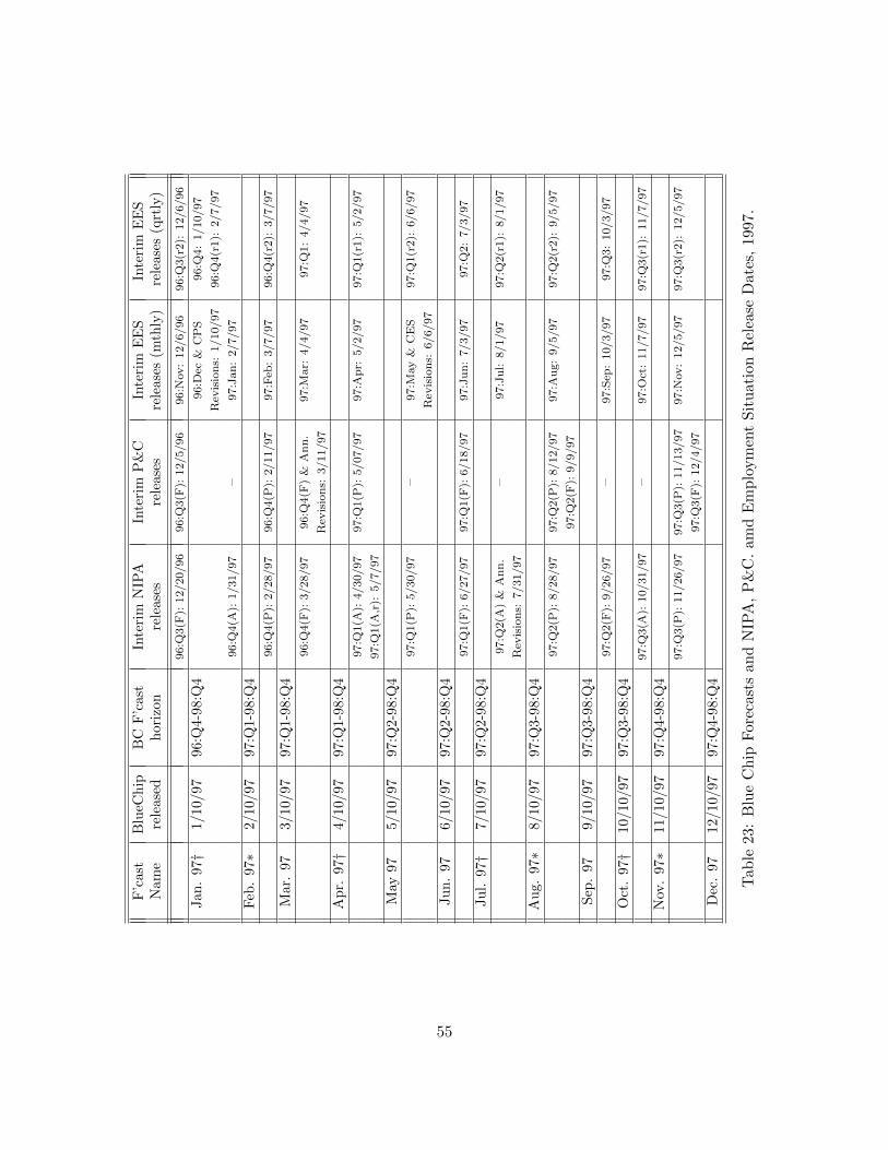
F’c

ast

Blu

eCh

ipB

CF

’cas

tIn

teri

mN

IPA

Inte

rim

P&

CIn

teri

mE

ES

Inte

rim

EE

SN

ame

rele

ased

hor

izon

rele

ase

sre

lease

sre

lease

s(m

thly

)re

lease

s(q

rtly

)

96:Q

3(F

):12/20/96

96:Q

3(F

):12/5/96

96:N

ov:12/6/96

96:Q

3(r2):

12/6/96

Jan

.97†

1/10

/97

96:Q

4-98

:Q4

96:D

ec&

CPS

96:Q

4:1/10/97

Rev

isions:

1/10/97

96:Q

4(r1):

2/7/97

96:Q

4(A

):1/31/97

–97:Jan:2/7/97

Feb

.97∗

2/10

/97

97:Q

1-98

:Q4

96:Q

4(P

):2/28/97

96:Q

4(P

):2/11/97

97:Feb

:3/7/97

96:Q

4(r2):

3/7/97

Mar

.97

3/10

/97

97:Q

1-98

:Q4

96:Q

4(F

):3/28/97

96:Q

4(F

)&

Ann.

97:M

ar:

4/4/97

97:Q

1:4/4/97

Rev

isions:

3/11/97

Ap

r.97†

4/10

/97

97:Q

1-98

:Q4

97:Q

1(A

):4/30/97

97:Q

1(P

):5/07/97

97:A

pr:

5/2/97

97:Q

1(r1):

5/2/97

97:Q

1(A

,r):

5/7/97

May

975/

10/9

797

:Q2-

98:Q

497:Q

1(P

):5/30/97

–97:M

ay&

CES

97:Q

1(r2):

6/6/97

Rev

isions:

6/6/97

Ju

n.

976/

10/9

797

:Q2-

98:Q

497:Q

1(F

):6/27/97

97:Q

1(F

):6/18/97

97:Jun:7/3/97

97:Q

2:7/3/97

Ju

l.97†

7/10

/97

97:Q

2-98

:Q4

97:Q

2(A

)&

Ann.

–97:Jul:

8/1/97

97:Q

2(r1):

8/1/97

Rev

isions:

7/31/97

Au

g.97∗

8/10

/97

97:Q

3-98

:Q4

97:Q

2(P

):8/28/97

97:Q

2(P

):8/12/97

97:A

ug:9/5/97

97:Q

2(r2):

9/5/97

97:Q

2(F

):9/9/97

Sep

.97

9/10

/97

97:Q

3-98

:Q4

97:Q

2(F

):9/26/97

–97:Sep

:10/3/97

97:Q

3:10/3/97

Oct

.97†

10/1

0/97

97:Q

3-98

:Q4

97:Q

3(A

):10/31/97

–97:O

ct:11/7/97

97:Q

3(r1):

11/7/97

Nov

.97∗

11/1

0/97

97:Q

4-98

:Q4

97:Q

3(P

):11/26/97

97:Q

3(P

):11/13/97

97:N

ov:12/5/97

97:Q

3(r2):

12/5/97

97:Q

3(F

):12/4/97

Dec

.97

12/1

0/97

97:Q

4-98

:Q4

Tab

le23:

Blu

eC

hip

For

ecas

tsan

dN

IPA

,P

&C

.am

dE

mp

loym

ent

Sit

uat

ion

Rel

ease

Dat

es,

1997

.

55

F’c

ast

Blu

eCh

ipB

CF

’cas

tIn

teri

mN

IPA

Inte

rim

P&

CIn

teri

mE

ES

Inte

rim

EE

SN

ame

rele

ased

hor

izon

rele

ase

sre

lease

sre

lease

s(m

thly

)re

lease

s(q

rtly

)

97:Q

3(F

):12/23/97

–97:D

ec&

CPS

97:Q

4:1/9/98

Rev

isions:

1/9/98

Jan

.98†

1/10

/98

97:Q

4-99

:Q4

97:Q

4(A

):1/30/98

–98:Jan:2/6/98

97:Q

4(r1):

2/6/98

Feb

.98

2/10

/98

98:Q

1-99

:Q4

97:Q

4(P

):2/10/98

97:Q

4(P

):2/27/98

–98:Feb

:3/6/98

97:Q

4(r2):

3/6/98

Mar

.98

3/10

/98

98:Q

1-99

:Q4

97:Q

4(F

)&

Ann.

Rev

isions:

3/10/98

97:Q

4(F

):3/26/98

–98:M

ar:

4/3/98

98:Q

1:4/3/98

Ap

r.98†

4/10

/98

98:Q

1-99

:Q4

98:Q

1(A

):4/30/98

98:Q

1(P

):5/07/98

98:A

pr:

5/8/98

98:Q

1(r1):

5/8/98

May

985/

10/9

898

:Q2-

99:Q

498:Q

1(P

):5/28/98

98:Q

1(F

):6/4/98

98:M

ay&

CES

98:Q

1(r2):

6/5/98

Rev

isions:

6/5/98

Ju

n.

986/

10/9

898

:Q2-

99:Q

498:Q

1(F

):6/25/98

–98:Jun:7/2/98

98:Q

2:7/2/98

Ju

l.98†

7/10

/98

98:Q

2-99

:Q4

98:Q

2(A

)&

Ann.

–98:Jul:

8/7/98

98:Q

2(r1):

8/7/98

Rev

isions:

7/31/98

Au

g.98∗

8/10

/98

98:Q

3-99

:Q4

98:Q

2(P

):8/27/98

98:Q

2(P

):8/11/98

98:A

ug:9/4/98

98:Q

2(r2):

9/4/98

98:Q

2(F

):9/3/98

Sep

.98

9/10

/98

98:Q

3-99

:Q4

98:Q

2(F

):9/24/98

–98:Sep

:10/2/98

98:Q

3:10/2/98

Oct

.98†

10/1

0/98

98:Q

3-99

:Q4

98:Q

3(A

):10/30/98

–98:O

ct:11/5/98

98:Q

3(r1):

11/5/98

Nov

.98

11/1

0/98

98:Q

4-99

:Q4

98:Q

3(P

):11/10/98

98:Q

3(P

):11/24/98

98:Q

3(F

):12/3/98

98:N

ov:12/4/98

98:Q

3(r2):

12/4/98

Dec

.98

12/1

0/98

98:Q

4-99

:Q4

Tab

le24:

Blu

eC

hip

For

ecas

tsan

dN

IPA

,P

&C

.am

dE

mp

loym

ent

Sit

uat

ion

Rel

ease

Dat

es,

1998

.

56

F’c

ast

Blu

eCh

ipB

CF

’cas

tIn

teri

mN

IPA

Inte

rim

P&

CIn

teri

mE

ES

Inte

rim

EE

SN

ame

rele

ased

hor

izon

rele

ase

sre

lease

sre

lease

s(m

thly

)re

lease

s(q

rtly

)

98:Q

3(F

):12/23/98

–98:D

ec&

CPS

98:Q

4:1/8/99

Rev

isions:

1/8/99

Jan

.99†

1/10

/99

98:Q

4-00

:Q4

98:Q

4(A

):1/29/99

98:Q

4(P

):2/9/99

99:Jan:2/5/99

98:Q

4(r1):

2/5/99

Feb

.99

2/10

/99

99:Q

1-00

:Q4

98:Q

4(P

):2/26/99

98:Q

4(F

)&

Ann.

99:Feb

:3/5/99

98:Q

4(r2):

3/5/99

Rev

isions:

3/9/99

Mar

.99

3/10

/99

99:Q

1-00

:Q4

98:Q

4(F

):3/31/99

–99:M

ar:

4/2/99

99:Q

1:4/2/99

Ap

r.99†

4/10

/99

99:Q

1-00

:Q4

99:Q

1(A

):4/30/99

–99:A

pr:

5/7/99

99:Q

1(r1):

5/7/99

May

99∗

5/10

/99

99:Q

2-00

:Q4

99:Q

1(P

):5/27/99

99:Q

1(P

):5/11/99

99:M

ay&

CES

99:Q

1(r2):

6/4/99

99:Q

1(F

):6/8/99

Rev

isions:

6/4/99

Ju

n.

996/

10/9

999

:Q2-

00:Q

499:Q

1(F

):6/25/99

–99:Jun:7/2/99

99:Q

2:7/2/99

Ju

l.99†

7/10

/99

99:Q

2-00

:Q4

99:Q

2(A

):7/29/99

99:Q

2(P

):8/5/99

99:Jul:

8/6/99

99:Q

2(r1):

8/6/99

Au

g.99

8/10

/99

99:Q

3-00

:Q4

99:Q

2(P

):8/26/99

99:Q

2(F

):9/2/99

99:A

ug:9/3/99

99:Q

2(r2):

9/3/99

Sep

.99

9/10

/99

99:Q

3-00

:Q4

99:Q

2(F

):9/30/99

–99:Sep

:10/8/99

99:Q

3:10/8/99

Oct

.99†

10/1

0/99

99:Q

3-00

:Q4

99:Q

3(A

)&

Comp.

–99:O

ct:11/5/99

99:Q

3(r1):

11/5/99

Rev

isions:

10/29/99

Nov

.99∗

11/1

0/99

99:Q

4-00

:Q4

99:Q

3(P

):11/24/99

99:Q

3(P

):11/12/99

99:N

ov:12/3/99

99:Q

3(r2):

12/3/99

99:Q

3(F

):12/7/99

Dec

.99

12/1

0/99

99:Q

4-00

:Q4

Tab

le25:

Blu

eC

hip

For

ecas

tsan

dN

IPA

,P

&C

.am

dE

mp

loym

ent

Sit

uat

ion

Rel

ease

Dat

es,

1999

.

57

F’c

ast

Blu

eCh

ipB

CF

’cas

tIn

teri

mN

IPA

Inte

rim

P&

CIn

teri

mE

ES

Inte

rim

EE

SN

ame

rele

ased

hor

izon

rele

ase

sre

lease

sre

lease

s(m

thly

)re

lease

s(q

rtly

)

99:Q

3(F

):12/22/99

–99:D

ec&

CPS

99:Q

4:1/7/00

Rev

isions:

1/7/00

Jan

.00†

1/10

/00

99:Q

4-01

:Q4

99:Q

4(A

):1/28/00

99:Q

4(P

):2/8/00

00:Jan:2/4/00

99:Q

4(r1):

2/4/00

Feb

.00

2/10

/00

00:Q

1-01

:Q4

99:Q

4(P

):2/25/00

99:Q

4(F

)&

Ann.

00:Feb

:3/3/00

99:Q

4(r2):

3/3/00

Rev

isions:

3/7/00

Mar

.00

3/10

/00

00:Q

1-01

:Q4

99:Q

4(F

):3/30/00

–00:M

ar:

4/7/00

00:Q

1:4/7/00

99:Q

4(F

,r):

4/3/00

Ap

r.00†

4/10

/00

00:Q

1-01

:Q4

00:Q

1(A

):4/27/00

00:Q

1(P

):5/4/00

00:A

pr:

5/5/00

00:Q

1(r1):

5/5/00

May

005/

10/0

000

:Q2-

01:Q

400:Q

1(P

):5/25/00

00:Q

1(F

):6/6/00

00:M

ay&

CES

00:Q

1(r2):

6/2/00

Rev

isions:

6/2/00

Ju

n.

006/

10/0

000

:Q2-

01:Q

400:Q

1(F

):6/29/00

–00:Jun:7/7/00

00:Q

2:7/7/00

Ju

l.00†

7/10

/00

00:Q

2-01

:Q4

00:Q

2(A

)&

Ann.

00:Q

2(P

)&

NIP

A00:Jul:

8/4/00

00:Q

2(r1):

8/4/00

Rev

isions:

7/28/00

Rev

isions:

8/8/00

Au

g.00

8/10

/00

00:Q

3-01

:Q4

00:Q

2(P

):8/25/00

00:Q

2(F

):9/6/00

00:A

ug:9/1/00

00:Q

2(r2):

9/1/00

Sep

.00

9/10

/00

00:Q

3-01

:Q4

00:Q

2(F

):9/28/00

–00:Sep

:10/6/00

00:Q

3:10/6/00

Oct

.00†

10/1

0/00

00:Q

3-01

:Q4

00:Q

3(A

):10/27/00

00:Q

3(P

):11/2/00

00:O

ct:11/3/00

00:Q

3(r1):

11/3/00

Nov

.00

11/1

0/00

00:Q

4-01

:Q4

00:Q

3(P

):11/29/00

00:Q

3(F

):12/6/00

00:N

ov:12/8/00

00:Q

3(r2):

12/8/00

Dec

.00

12/1

0/00

00:Q

4-01

:Q4

Tab

le26:

Blu

eC

hip

For

ecas

tsan

dN

IPA

,P

&C

.am

dE

mp

loym

ent

Sit

uat

ion

Rel

ease

Dat

es,

2000

.

58

F’c

ast

Blu

eCh

ipB

CF

’cas

tIn

teri

mN

IPA

Inte

rim

P&

CIn

teri

mE

ES

Inte

rim

EE

SN

ame

rele

ased

hor

izon

rele

ase

sre

lease

sre

lease

s(m

thly

)re

lease

s(q

rtly

)

00:Q

3(F

):12/21/00

–00:D

ec&

CPS

00:Q

4:1/5/01

Rev

isions:

1/5/01

Jan

.01†

1/10

/01

00:Q

4-02

:Q4

00:Q

4(A

):1/31/01

00:Q

4(P

):2/7/01

01:Jan:2/2/01

00:Q

4(r1):

2/2/01

Feb

.01

2/10

/01

01:Q

1-02

:Q4

00:Q

4(P

):2/28/01

00:Q

4(F

)&

Ann.

01:Feb

:3/9/01

00:Q

4(r2):

3/9/01

Rev

isions:

3/6/01

Mar

.01

3/10

/01

01:Q

1-02

:Q4

00:Q

4(F

):3/29/01

–01:M

ar:

4/6/01

01:Q

1:4/6/01

Ap

r.01†

4/10

/01

01:Q

1-02

:Q4

01:Q

1(A

):4/27/01

01:Q

1(P

):5/8/01

01:A

pr:

5/4/01

01:Q

1(r1):

5/4/01

May

015/

10/0

101

:Q2-

02:Q

401:Q

1(P

):5/25/01

01:Q

1(F

):6/5/01

01:M

ay&

CES

01:Q

1(r2):

6/1/01

Rev

isions:

6/1/01

Ju

n.

016/

10/0

101

:Q2-

02:Q

401:Q

1(F

):6/29/01

–01:Jun:7/6/01

01:Q

2:7/6/01

Ju

l.01†

7/10

/01

01:Q

2-02

:Q4

01:Q

2(A

)&

Ann.

01:Q

2(P

)&

NIP

A01:Jul:

8/3/01

01:Q

2(r1):

8/3/01

Rev

isions:

7/27/01

Rev

isions:

8/7/01

Au

g.01

8/10

/01

01:Q

3-02

:Q4

01:Q

2(P

):8/29/01

01:Q

2(F

):9/5/01

01:A

ug:9/7/01

01:Q

2(r2):

9/7/01

Sep

.01

9/10

/01

01:Q

3-02

:Q4

01:Q

2(F

):9/28/01

–01:Sep

:10/5/01

01:Q

3:10/5/01

Oct

.01†

10/1

0/01

01:Q

3-02

:Q4

01:Q

3(A

):10/31/01

01:Q

3(P

):11/7/01

01:O

ct:11/2/01

01:Q

3(r1):

11/2/01

Nov

.01

11/1

0/01

01:Q

4-02

:Q4

01:Q

3(P

):11/30/01

01:Q

3(F

):12/6/01

01:N

ov:12/7/01

01:Q

3(r2):

12/7/01

Dec

.01

12/1

0/01

01:Q

4-02

:Q4

Tab

le27:

Blu

eC

hip

For

ecas

tsan

dN

IPA

,P

&C

.am

dE

mp

loym

ent

Sit

uat

ion

Rel

ease

Dat

es,

2001

.

59

F’c

ast

Blu

eCh

ipB

CF

’cas

tIn

teri

mN

IPA

Inte

rim

P&

CIn

teri

mE

ES

Inte

rim

EE

SN

ame

rele

ased

hor

izon

rele

ase

sre

lease

sre

lease

s(m

thly

)re

lease

s(q

rtly

)

01:Q

3(F

):12/21/01

–01:D

ec&

CPS

01:Q

4:1/4/02

Rev

isions:

1/4/02

Jan

.02†

1/10

/02

02:Q

4-03

:Q4

01:Q

4(A

):1/30/02

01:Q

4(P

):2/6/02

02:Jan:2/1/01

01:Q

4(r1):

2/1/02

Feb

.02

2/10

/02

02:Q

1-03

:Q4

01:Q

4(P

):2/28/02

01:Q

4(F

)&

Ann.

02:Feb

:3/8/02

01:Q

4(r2):

3/8/02

Rev

isions:

3/7/02

Mar

.02

3/10

/02

02:Q

1-03

:Q4

01:Q

4(F

):3/28/02

–02:M

ar:

4/5/02

02:Q

1:4/5/02

Ap

r.02†

4/10

/02

02:Q

1-03

:Q4

02:Q

1(A

):4/26/02

02:Q

1(P

):5/7/02

02:A

pr:

5/3/02

02:Q

1(r1):

5/3/02

May

025/

10/0

202

:Q2-

03:Q

402:Q

1(P

):5/24/02

02:Q

1(F

):5/31/02

02:M

ay&

CES

02:Q

1(r2):

6/7/02

Rev

isions:

6/7/02

Ju

n.

026/

10/0

202

:Q2-

03:Q

402:Q

1(F

):6/27/02

–02:Jun:7/5/02

02:Q

2:7/5/02

Ju

l.02†

7/10

/02

02:Q

2-03

:Q4

02:Q

2(A

)&

Ann.

02:Q

2(P

)&

NIP

A02:Jul:

8/2/02

02:Q

2(r1):

8/2/02

Rev

isions:

7/31/02

Rev

isions:

8/9/02

Au

g.02

8/10

/02

02:Q

3-03

:Q4

02:Q

2(P

):8/29/02

02:Q

2(F

):9/5/02

02:A

ug:9/6/02

02:Q

2(r2):

9/6/02

Sep

.02

9/10

/02

02:Q

3-03

:Q4

02:Q

2(F

):9/27/02

–02:Sep

:10/4/02

02:Q

3:10/4/02

Oct

.02†

10/1

0/02

02:Q

3-03

:Q4

02:Q

3(A

):10/31/02

02:Q

3(P

):11/7/02

02:O

ct:11/1/02

02:Q

3(r1):

11/1/02

Nov

.02

11/1

0/02

02:Q

4-03

:Q4

02:Q

3(P

):11/26/02

02:Q

3(F

):12/4/02

02:N

ov:12/6/02

02:Q

3(r2):

12/6/02

Dec

.02

12/1

0/02

02:Q

4-03

:Q4

Tab

le28:

Blu

eC

hip

For

ecas

tsan

dN

IPA

,P

&C

.am

dE

mp

loym

ent

Sit

uat

ion

Rel

ease

Dat

es,

2002

.

60

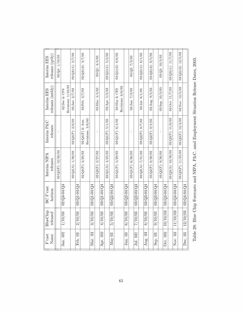
F’c

ast

Blu

eCh

ipB

CF

’cas

tIn

teri

mN

IPA

Inte

rim

P&

CIn

teri

mE

ES

Inte

rim

EE

SN

ame

rele

ased

hor

izon

rele

ase

sre

lease

sre

lease

s(m

thly

)re

lease

s(q

rtly

)

02:Q

3(F

):12/20/02

–02:Q

4:1/10/03

Jan

.03†

1/10

/03

02:Q

4-04

:Q4

02:D

ec&

CPS

Rev

isions:

1/10/03

02:Q

4(A

):1/30/03

02:Q

4(P

):2/6/03

03:Jan:2/7/03

02:Q

4(r1):

2/7/03

Feb

.03

2/10

/03

03:Q

1-04

:Q4

02:Q

4(P

):2/28/03

02:Q

4(F

)&

Ann.

03:Feb

:3/7/03

02:Q

4(r2):

3/7/03

Rev

isions:

3/6/03

Mar

.03

3/10

/03

03:Q

1-04

:Q4

02:Q

4(F

):3/27/03

–03:M

ar:

4/4/03

03:Q

1:4/4/03

Ap

r.03†

4/10

/03

03:Q

1-04

:Q4

03:Q

1(A

):4/25/03

03:Q

1(P

):5/1/03

03:A

pr:

5/2/03

03:Q

1(r1):

5/2/03

May

035/

10/0

303

:Q2-

04:Q

403:Q

1(P

):5/29/03

03:Q

1(F

):6/4/03

03:M

ay&

CES

03:Q

1(r2):

6/6/03

Rev

isions:

6/6/03

Ju

n.

036/

10/0

303

:Q2-

04:Q

403:Q

1(F

):6/26/03

–03:Jun:7/3/03

03:Q

2:7/3/03

Ju

l.03†

7/10

/03

03:Q

2-04

:Q4

03:Q

2(A

):7/31/03

03:Q

2(P

):8/7/03

03:Jul:

8/1/03

03:Q

2(r1):

8/1/03

Au

g.03

8/10

/03

03:Q

3-04

:Q4

03:Q

2(P

):8/28/03

03:Q

2(F

):9/4/03

03:A

ug:9/5/03

03:Q

2(r2):

9/5/03

Sep

.03

9/10

/03

03:Q

3-04

:Q4

03:Q

2(F

):9/26/03

–03:Sep

:10/3/03

03:Q

3:10/3/03

Oct

.03†

10/1

0/03

03:Q

3-04

:Q4

03:Q

3(A

):10/30/03

03:Q

3(P

):11/6/03

03:O

ct:11/7/03

03:Q

3(r1):

11/7/03

Nov

.03

11/1

0/03

03:Q

4-04

:Q4

03:Q

3(P

):11/25/03

03:Q

3(F

):12/3/03

03:N

ov:12/5/03

03:Q

3(r2):

12/5/03

Dec

.03

12/1

0/03

03:Q

4-04

:Q4

Tab

le29:

Blu

eC

hip

For

ecas

tsan

dN

IPA

,P

&C

.am

dE

mp

loym

ent

Sit

uat

ion

Rel

ease

Dat

es,

2003

.

61

F’c

ast

Blu

eCh

ipB

CF

’cas

tIn

teri

mN

IPA

Inte

rim

P&

CIn

teri

mE

ES

Inte

rim

EE

SN

ame

rele

ased

hori

zon

rele

ase

sre

lease

sre

lease

s(m

thly

)re

lease

s(q

rtly

)

Comp.Rev

.:12/10/03

–03:D

ec&

CPS

03:Q

4:1/9/04

03:Q

3(F

):12/23/03

–Rev

isions:

1/9/04

Jan

.04†

1/10

/04

03:Q

4-05

:Q4

03:Q

4(A

):1/30/04

03:Q

4(P

):2/5/04

04:Jan&

CES

03:Q

4(r1):

2/6/04

Rev

isions:

2/6/06

Feb

.04

2/10

/04

04:Q

1-05

:Q4

03:Q

4(P

):2/27/04

03:Q

4(F

)&

Ann.

04:Feb

:3/5/04

03:Q

4(r2):

3/5/04

Rev

isions:

3/4/04

Mar

.04

3/10

/04

04:Q

1-05

:Q4

07:Q

4(F

):3/25/04

–04:M

ar:

4/2/04

04:Q

1:4/2/04

Ap

r.04†

4/10

/04

04:Q

1-05

:Q4

04:Q

1(A

):4/29/04

04:Q

1(P

):5/6/04

04:A

pr:

5/7/04

04:Q

1(r1):

5/7/04

May

045/

10/0

404

:Q2-

05:Q

404:Q

1(P

):5/27/04

04:Q

1(F

):6/3/04

04:M

ay:6/4/04

04:Q

1(r2):

6/4/04

Ju

n.

046/

10/0

404

:Q2-

05:Q

404:Q

1(F

):6/25/04

–04:Jun:7/2/04

04:Q

2:7/2/04

Ju

l.04†

7/10

/04

04:Q

2-05

:Q4

04:Q

2(A

)&

Ann.

–04:Jul:

8/6/04

04:Q

2(r1):

8/6/04

Rev

ision:7/30/04

Au

g.04

8/10

/04

04:Q

3-05

:Q4

04:Q

2(P

)&

NIP

A

Rev

ision:8/10/04

04:Q

2(P

):8/27/04

04:Q

2(F

):9/2/04

04:A

ug:9/3/04

04:Q

2(r2):

9/3/04

Sep

.04

9/10

/04

04:Q

3-05

:Q4

04:Q

2(F

):9/29/04

–04:Sep

:10/8/04

04:Q

3:10/8/04

Oct

.04†

10/1

0/04

04:Q

3-05

:Q4

04:Q

3(A

):10/29/04

04:Q

2(E

rr.):10/13/04

04:O

ct:11/5/04

04:Q

3(r1):

11/5/04

04:Q

3(P

):11/4/04

Nov

.04

11/1

0/04

04:Q

4-05

:Q4

04:Q

3(P

):11/30/04

04:Q

3(F

):12/7/04

04:N

ov:12/3/04

04:Q

3(r2):

12/3/04

Dec

.04

12/1

0/04

04:Q

4-05

:Q4

Tab

le30:

Blu

eC

hip

For

ecas

tsan

dN

IPA

,P

&C

.am

dE

mp

loym

ent

Sit

uat

ion

Rel

ease

Dat

es,

2004

.

62

F’c

ast

Blu

eCh

ipB

CF

’cas

tIn

teri

mN

IPA

Inte

rim

P&

CIn

teri

mE

ES

Inte

rim

EE

SN

ame

rele

ased

hor

izon

rele

ase

sre

lease

sre

lease

s(m

thly

)re

lease

s(q

rtly

)

04:Q

3(F

):12/22/04

04:Q

3(F

):12/7/04

04:D

ec&

CPS

04:Q

4:1/7/05

Rev

isions:

1/7/05

Jan

.05†

1/10

/05

04:Q

4-06

:Q4

04:Q

4(A

):1/28/05

04:Q

4(P

):2/3/05

05:Jan&

CES

04:Q

4(r1):

2/4/05

Rev

isions:

2/4/05

Feb

.05

2/10

/05

05:Q

1-06

:Q4

04:Q

4(P

):2/25/05

04:Q

4(F

)&

Ann.

05:Feb

:3/4/05

04:Q

4(r2):

3/4/05

Rev

isions:

3/3/05

Mar

.05

3/10

/05

05:Q

1-06

:Q4

04:Q

4(F

):3/30/05

–05:M

ar:

4/1/05

05:Q

1:4/1/05

Ap

r.05†

4/10

/05

05:Q

1-06

:Q4

05:Q

1(A

):4/28/05

05:Q

1(P

):5/5/05

05:A

pr:

5/6/05

05:Q

1(r1):

5/6/05

May

055/

10/0

505

:Q2-

06:Q

405:Q

1(P

):5/26/05

05:Q

1(F

):6/2/05

05:M

ay:6/3/05

05:Q

1(r2):

6/3/05

Ju

n.

056/

10/0

505

:Q2-

06:Q

405:Q

1(F

):6/29/05

–05:Jun:7/8/05

05:Q

2:7/8/05

Ju

l.05†

7/10

/05

05:Q

2-06

:Q4

05:Q

2(A

)&

Ann.

05:Q

2(P

)&

NIP

A05:Jul:

8/5/05

05:Q

2(r1):

8/5/05

Rev

isions:

7/29/05

Rev

isions:

8/9/05

Au

g.05

8/10

/05

05:Q

3-06

:Q4

05:Q

2(P

):8/31/05

05:Q

2(F

):9/7/05

05:A

ug:9/2/05

05:Q

2(r2):

9/2/05

Sep

.05

9/10

/05

05:Q

3-06

:Q4

05:Q

2(F

):9/29/05

–05:Sep

:10/7/05

05:Q

3:10/7/05

Oct

.05†

10/1

0/05

05:Q

3-06

:Q4

05:Q

3(A

):10/28/05

05:Q

3(P

):11/3/05

05:O

ct:11/4/05

05:Q

3(r1):

11/4/05

Nov

.05

11/1

0/05

05:Q

4-06

:Q4

05:Q

3(P

):11/30/05

05:Q

3(F

):12/6/05

05:N

ov:12/2/05

05:Q

3(r2):

12/2/05

Dec

.05

12/1

0/05

05:Q

4-06

:Q4

Tab

le31:

Blu

eC

hip

For

ecas

tsan

dN

IPA

,P

&C

.am

dE

mp

loym

ent

Sit

uat

ion

Rel

ease

Dat

es,

2005

.

63

F’c

ast

Blu

eCh

ipB

CF

’cas

tIn

teri

mN

IPA

Inte

rim

P&

CIn

teri

mE

ES

Inte

rim

EE

SN

ame

rele

ased

hor

izon

rele

ase

sre

lease

sre

lease

s(m

thly

)re

lease

s(q

rtly

)

05:Q

3(F

):12/21/05

–05:D

ec&

CPS

05:Q

4:1/6/06

Rev

isions:

1/6/06

Jan

.06†

1/10

/06

05:Q

4-07

:Q4

05:Q

4(A

):1/27/06

05:Q

4(P

):2/2/06

06:Jan&

CES

05:Q

4(r1):

2/3/06

Rev

isions:

2/3/06

Feb

.06

2/10

/06

06:Q

1-07

:Q4

05:Q

4(P

):2/28/06

05:Q

4(F

)&

Ann.

Rev

isions:

3/7/06

Mar

.06

3/10

/06

06:Q

1-07

:Q4

06:Feb

:3/10/06

05:Q

4(r2):

3/10/06

05:Q

4(F

):3/30/06

–06:M

ar:

4/7/06

06:Q

1:4/7/06

Ap

r.06†

4/10

/06

06:Q

1-07

:Q4

06:Q

1(A

):4/28/06

06:Q

1(P

):5/4/06

06:A

pr:

5/5/06

06:Q

1(r1):

5/5/06

May

065/

10/0

606

:Q2-

07:Q

406:Q

1(P

):5/25/06

06:Q

1(F

):6/1/06

06:M

ay:6/2/06

06:Q

1(r2):

6/2/06

Ju

n.

066/

10/0

606

:Q2-

07:Q

406:Q

1(F

):6/29/06

–06:Jun:7/7/06

06:Q

2:7/7/06

Ju

l.06†

7/10

/06

06:Q

2-07

:Q4

06:Q

2(A

)&

Ann.

06:Q

2(P

)&

NIP

A06:Jul:

8/4/06

06:Q

2(r1):

8/4/06

Rev

isions:

7/28/06

Rev

isions:

8/8/06

Au

g.06

8/10

/06

06:Q

3-07

:Q4

06:Q

2(P

):8/30/06

06:Q

2(F

):9/6/06

06:A

ug:9/1/06

06:Q

2(r2):

9/1/06

Sep

.06

9/10

/06

06:Q

3-07

:Q4

06:Q

2(F

):9/28/06

–06:Sep

:10/6/06

06:Q

3:10/6/06

Oct

.06†

10/1

0/06

06:Q

3-07

:Q4

06:Q

3(A

):10/27/06

06:Q

3(P

):11/2/06

06:O

ct:11/3/06

06:Q

3(r1):

11/3/06

Nov

.06

11/1

0/06

06:Q

4-07

:Q4

06:Q

3(P

):11/29/06

06:Q

3(F

):12/5/06

06:N

ov:12/8/06

06:Q

3(r2):

12/8/06

Dec

.06

12/1

0/06

06:Q

4-07

:Q4

Tab

le32:

Blu

eC

hip

For

ecas

tsan

dN

IPA

,P

&C

.am

dE

mp

loym

ent

Sit

uat

ion

Rel

ease

Dat

es,

2006

.

64

F’c

ast

Blu

eCh

ipB

CF

’cas

tIn

teri

mN

IPA

Inte

rim

P&

CIn

teri

mE

ES

Inte

rim

EE

SN

ame

rele

ased

hor

izon

rele

ase

sre

lease

sre

lease

s(m

thly

)re

lease

s(q

rtly

)

06:Q

3(F

):12/21/06

–06:D

ec&

CPS

06:Q

4:1/5/07

Rev

isions:

1/5/07

Jan

.07†

1/10

/07

06:Q

4-08

:Q4

06:Q

4(A

):1/31/07

06:Q

4(P

):2/7/07

07:Jan&

CES

06:Q

4(r1):

2/2/07

Rev

isions:

2/2/07

Feb

.07

2/10

/07

07:Q

1-08

:Q4

06:Q

4(P

):2/28/07

06:Q

4(F

)&

Ann.

07:Feb

:3/9/07

06:Q

4(r2):

3/9/07

Rev

isions:

3/6/07

Mar

.07

3/10

/07

07:Q

1-08

:Q4

06:Q

4(F

):3/29/07

–07:M

ar:

4/6/07

07:Q

1:4/6/07

Ap

r.07†

4/10

/07

07:Q

1-08

:Q4

07:Q

1(A

):4/27/07

07:Q

1(P

):5/3/07

07:A

pr:

5/4/07

07:Q

1(r1):

5/4/07

May

075/

10/0

707

:Q2-

08:Q

407:Q

1(P

):5/31/07

07:Q

1(F

):6/6/07

07:M

ay:6/1/07

07:Q

1(r2):

6/1/07

Ju

n.

076/

10/0

707

:Q2-

08:Q

407:Q

1(F

):6/28/07

–07:Jun:7/6/07

07:Q

2:7/6/07

Ju

l.07†

7/10

/07

07:Q

2-08

:Q4

07:Q

2(A

)&

Ann.

07:Q

2(P

)&

NIP

A07:Jul:

8/3/07

07:Q

2(r1):

8/3/07

Rev

isions:

7/27/07

Rev

isions:

8/7/07

Au

g.07

8/10

/07

07:Q

3-08

:Q4

07:Q

2(P

):8/30/07

07:Q

2(F

):9/6/07

07:A

ug:9/7/07

07:Q

2(r2):

9/7/07

Sep

.07

9/10

/07

07:Q

3-08

:Q4

07:Q

2(F

):9/27/07

–07:Sep

:10/5/07

07:Q

3:10/5/07

Oct

.07†

10/1

0/07

07:Q

3-08

:Q4

07:Q

3(A

):10/31/07

07:Q

3(P

):11/7/07

07:O

ct:11/2/07

07:Q

3(r1):

11/2/07

Nov

.07

11/1

0/07

07:Q

4-08

:Q4

07:Q

3(P

):11/29/07

07:Q

3(F

):12/5/07

07:N

ov:12/7/07

07:Q

3(r2):

12/7/07

Dec

.07

12/1

0/07

07:Q

4-08

:Q4

Tab

le33:

Blu

eC

hip

For

ecas

tsan

dN

IPA

,P

&C

.am

dE

mp

loym

ent

Sit

uat

ion

Rel

ease

Dat

es,

2007

.

65

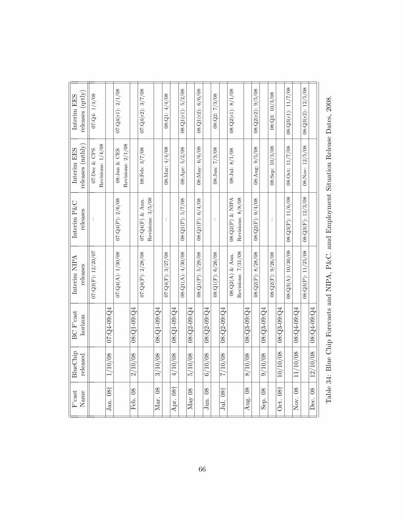
F’c

ast

Blu

eCh

ipB

CF

’cas

tIn

teri

mN

IPA

Inte

rim

P&

CIn

teri

mE

ES

Inte

rim

EE

SN

ame

rele

ased

hor

izon

rele

ase

sre

lease

sre

lease

s(m

thly

)re

lease

s(q

rtly

)

07:Q

3(F

):12/20/07

–07:D

ec&

CPS

07:Q

4:1/4/08

Rev

isions:

1/4/08

Jan

.08†

1/10

/08

07:Q

4-09

:Q4

07:Q

4(A

):1/30/08

07:Q

4(P

):2/6/08

08:Jan&

CES

07:Q

4(r1):

2/1/08

Rev

isions:

2/1/08

Feb

.08

2/10

/08

08:Q

1-09

:Q4

07:Q

4(P

):2/28/08

07:Q

4(F

)&

Ann.

08:Feb

:3/7/08

07:Q

4(r2):

3/7/08

Rev

isions:

3/5/08

Mar

.08

3/10

/08

08:Q

1-09

:Q4

07:Q

4(F

):3/27/08

–08:M

ar:

4/4/08

08:Q

1:4/4/08

Ap

r.08†

4/10

/08

08:Q

1-09

:Q4

08:Q

1(A

):4/30/08

08:Q

1(P

):5/7/08

08:A

pr:

5/2/08

08:Q

1(r1):

5/2/08

May

085/

10/0

808

:Q2-

09:Q

408:Q

1(P

):5/29/08

08:Q

1(F

):6/4/08

08:M

ay:6/6/08

08:Q

1(r2):

6/6/08

Ju

n.

086/

10/0

808

:Q2-

09:Q

408:Q

1(F

):6/26/08

–08:Jun:7/3/08

08:Q

2:7/3/08

Ju

l.08†

7/10

/08

08:Q

2-09

:Q4

08:Q

2(A

)&

Ann.

08:Q

2(P

)&

NIP

A08:Jul:

8/1/08

08:Q

2(r1):

8/1/08

Rev

isions:

7/31/08

Rev

isions:

8/8/08

Au

g.08

8/10

/08

08:Q

3-09

:Q4

08:Q

2(P

):8/28/08

08:Q

2(F

):9/4/08

08:A

ug:9/5/08

08:Q

2(r2):

9/5/08

Sep

.08

9/10

/08

08:Q

3-09

:Q4

08:Q

2(F

):9/26/08

–08:Sep

:10/3/08

08:Q

3:10/3/08

Oct

.08†

10/1

0/08

08:Q

3-09

:Q4

08:Q

3(A

):10/30/08

08:Q

3(P

):11/6/08

08:O

ct:11/7/08

08:Q

3(r1):

11/7/08

Nov

.08

11/1

0/08

08:Q

4-09

:Q4

08:Q

3(P

):11/25/08

08:Q

3(F

):12/3/08

08:N

ov:12/5/08

08:Q

3(r2):

12/5/08

Dec

.08

12/1

0/08

08:Q

4-09

:Q4

Tab

le34:

Blu

eC

hip

For

ecas

tsan

dN

IPA

,P

&C

.am

dE

mp

loym

ent

Sit

uat

ion

Rel

ease

Dat

es,

2008

.

66

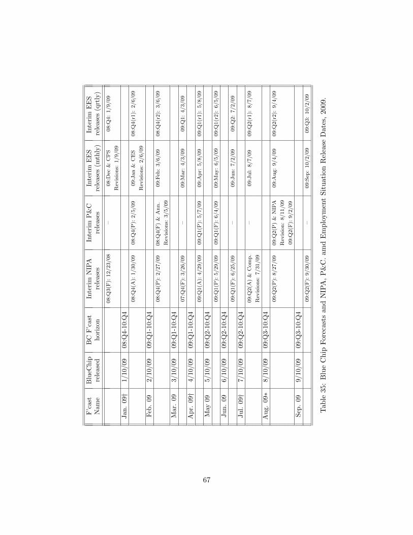
F’c

ast

Blu

eCh

ipB

CF

’cast

Inte

rim

NIP

AIn

teri

mP

&C

Inte

rim

EE

SIn

teri

mE

ES

Nam

ere

leas

edh

oriz

on

rele

ase

sre

lease

sre

lease

s(m

thly

)re

lease

s(q

rtly

)

08:Q

3(F

):12/23/08

–08:D

ec&

CPS

08:Q

4:1/9/09

Rev

isions:

1/9/09

Jan

.09†

1/10

/09

08:Q

4-10

:Q4

08:Q

4(A

):1/30/09

08:Q

4(P

):2/5/09

09:Jan&

CES

08:Q

4(r1):

2/6/09

Rev

isions:

2/6/09

Feb

.09

2/10

/09

09:Q

1-10

:Q4

08:Q

4(P

):2/27/09

08:Q

4(F

)&

Ann.

09:Feb

:3/6/09

08:Q

4(r2):

3/6/09

Rev

isions:

3/5/09

Mar

.09

3/10

/09

09:Q

1-10

:Q4

07:Q

4(F

):3/26/09

–09:M

ar:

4/3/09

09:Q

1:4/3/09

Ap

r.09†

4/10

/09

09:Q

1-10

:Q4

09:Q

1(A

):4/29/09

09:Q

1(P

):5/7/09

09:A

pr:

5/8/09

09:Q

1(r1):

5/8/09

May

09

5/10

/09

09:Q

2-10

:Q4

09:Q

1(P

):5/29/09

09:Q

1(F

):6/4/09

09:M

ay:6/5/09

09:Q

1(r2):

6/5/09

Ju

n.

096/

10/0

909

:Q2-

10:Q

409:Q

1(F

):6/25/09

–09:Jun:7/2/09

09:Q

2:7/2/09

Ju

l.09†

7/10

/09

09:Q

2-10

:Q4

09:Q

2(A

)&

Comp.

–09:Jul:

8/7/09

09:Q

2(r1):

8/7/09

Rev

isions:

7/31/09

Au

g.09∗

8/10

/09

09:Q

3-10

:Q4

09:Q

2(P

):8/27/09

09:Q

2(P

)&

NIP

A09:A

ug:9/4/09

09:Q

2(r2):

9/4/09

Rev

ision:8/11/09

09:Q

2(F

):9/2/09

Sep

.09

9/10

/09

09:Q

3-10

:Q4

09:Q

2(F

):9/30/09

–09:Sep

:10/2/09

09:Q

3:10/2/09

Tab

le35:

Blu

eC

hip

For

ecas

tsan

dN

IPA

,P

&C

.am

dE

mp

loym

ent

Sit

uat

ion

Rel

ease

Dat

es,

2009

.

67