How to save the planet? A state space model approach

Team 1

Abstract

Climate change is nowadays a key topic of interest in political discussions. It is crucial tohave proper models and perform accurate forecasts of climate-related variables to efficientlytackle the issues that climate change brings. This paper focuses on two aspects: the sensitivityof global CO2 atmospheric concentration forecasts to changes in CO2 emissions in differentregions of the world and how such changes in emissions can be achieved. We propose a statespace approach that takes into account the measurement errors to which climate data is subject.The model is based on the Global Carbon Budget Equation and allows to jointly estimate andforecast all the unobserved components driving the observed variables of the Budget Equationand CO2 atmospheric concentrations. It also has the flexibility to model the CO2 emissionsfor a group of countries. We further extend the state space model in order to allow the lat-ter emissions to depend on an indicator of economic activity for the region investigated. Wecompare our forecast from 2019 to 2100 to Representative Concentration Pathways (RCP) thatcorrespond to distinct scenarios leading to different temperature increases above pre-industriallevels. We find that a decrease in the EU28 CO2 emissions seems to have a bigger impactin reducing future CO2 concentration than changes in the US or non-OECD CO2 emissions.While we do not find a significant difference between the effects of CO2 emission changes fordeveloped and developing countries, a limitation may arise with respect to rooms for policiesin the latter. Furthermore, focusing on the US, our model indicates that CO2 emissions reactpositively with a magnitude 3 times higher than the change in production. It suggests that,given all external factors constant, CO2 emissions could be reduced by a half by 2040 if pro-duction was gradually decreased by 2.5% per yer, hence, without harming economic activity.

Keywords: Global Carbon Budget Equation, CO2 Atmospheric Concentration, State SpaceModels, Forecasting, Territorial Emissions, Economic Activity.

Contents1 Introduction 2

2 The Global Carbon Budget and territorial emissions 3

3 Data 4

4 A state space model approach 6

5 Results 85.1 Estimation . . . . . . . . . . . . . . . . . . . . . . . . . . . . . . . . . . . . . . . 85.2 Forecasts scenarios . . . . . . . . . . . . . . . . . . . . . . . . . . . . . . . . . . 85.3 Sensitivity Analysis . . . . . . . . . . . . . . . . . . . . . . . . . . . . . . . . . . 115.4 CO2 emissions and economic activity . . . . . . . . . . . . . . . . . . . . . . . . 14

6 Discussion 19

7 Conclusion 20

Appendices 24

1

1 IntroductionOver the last two decades, the Carbon Budget has been a problem of great interest, especially afterthe Earth Summit in Rio de Janeiro in 1992, where the member states of the United Nations de-cided to stick together to handle the conflict relating to sustainability and global warming. Aware-ness regarding climate change increased and it became clear that the need for understanding therelationship between carbon dioxide (hereafter CO2) emissions, land and ocean sinks and CO2 at-mospheric growth is critical. The problems were again emphasized at the COP21 in Paris, at whichpresent States agreed to keep the global temperature increase below 2 degrees above pre-industriallevel. However, unlike its predecessor, the Kyoto Protocol, which sets commitment targets thathave legal force, the Paris Agreement, with its emphasis on consensus-building, allows for volun-tary and nationally determined targets. The specific climate goals are thus politically encouraged,rather than legally bound. Climate change is however a global matter and the actions of one coun-try clearly have worldwide repercussions. To efficiently tackle global warming, new policies needto be established, and most importantly, policies between countries need to be aligned. Hence, notonly is it essential to understand historical and recent climate variations, it is also necessary to per-form reliable forecasts to compare potential future scenarios of various environmental variables,globally and across countries.

The growth rate of atmospheric CO2 is the largest human contributor to human-induced climatechange and it is increasing rapidly. It is crucial to have a proper understanding of the global carboncycle and to have accurate measurements of CO2 emissions and their redistribution among theatmosphere, ocean, and terrestrial biospheres. The carbon cycle implies that the amount of emittedCO2 that is not absorbed by the land or the ocean sinks must end up in the atmosphere. Hence, theequilibrium condition is as such,

Gt = EFFt + ELU

t − SLDt − SOCt ,

where Gt is the growth in atmospheric CO2 concentration, EFFt are CO2 emissions from fossil

fuels combustion and industrial processes, ELUt are the CO2 emissions from land-use change (e.g.

deforestation), SLDt is how much of these emissions are absorbed by the terrestrial biosphere andSOCt is the amount absorbed by oceans (Le Quere et al., 2018). However, each variable is measuredfrom different environmental models and the construction of each variable is hence subject tomeasurement errors. In practice, this leads to a significant discrepancy between the right and lefthand sides of the identity, implying a disequilibrium in the carbon cycle. The Global CarbonProject aims at quantifying this discrepancy (denoted by εt) by means of the so called GlobalCarbon Budget Equation,

Gt = EFFt + ELU

t − SLDt − SOCt + εt. (1)

It is however impossible to disentangle whether a positive imbalance for instance is induced by anoverestimation of emissions, an underestimation of the sinks absorption or an overestimation ofthe growth of atmospheric CO2 concentration.

The rise of interdisciplinary techniques and mostly the use of econometric methods have beenof interest in the recent years as similar problems have been observed in economic applications.

2

The aim of this paper is to model the sensitivity of global CO2 atmospheric concentration forecaststo changes in CO2 emissions in different regions of the world and how such changes in emissionscan be achieved, by means of an econometric approach. We propose a state space model that takesinto account the measurement errors to which climate data is subject. It is built upon the GlobalCarbon Budget Equation. It allows to jointly estimate and forecast the state variables of all theobservable variables that appear in the Carbon Budget Equation as well as the CO2 atmosphericconcentrations. We divide worldwide emissions into a region’s emissions and that of the rest ofthe world, to investigate the individual effects on global CO2 atmospheric concentration of suchregion. We further extend the state space model in order to allow the regional CO2 emissions todepend on an indicator of economic activity for the region investigated.

The paper is organized as follows, Section 2 highlights the motivations and the necessity of aneconometric model for the Carbon Budget that incorporates the individual effects of the emissionsof specific countries or groups of countries. Then, the paper describes the data set used in thisresearch. Section 4 presents the construction of the state-space model based on the Global CarbonBudget. Estimation of the model between 1959 and 2017, forecasts up to 2100 and a sensitivityanalysis that considers the individual country effects and the relation between US emissions andthe production index are performed in Section 5. Section 6 discusses the limitations and the pos-sible further research that this paper sheds light on, before concluding in Section 7.

2 The Global Carbon Budget and territorial emissionsThe Global Carbon Budget states that all CO2 emissions must either end up in the Earth’s sinksor in the atmosphere, while accounting for potential measurement errors. The traditional approachto model the growth of atmospheric CO2 concentration has been related to the field of physicsand climatology (Le Quere et al., 2018). Each variable in the Budget Equation (1) is measuredwith distinct – usually – climatology models and the imbalance is then simply constructed as thediscrepancy between the measured atmospheric CO2 concentration growth and the one implied bythe difference between emissions and Earth absorption.

Measurements errors associated with CO2 measurements and emission estimates still limit ourconfidence in calculating net carbon uptake from the atmosphere by the land and ocean (Ballantyneet al., 2015). As we enter into an era in which scientists are expected to provide an increasinglymore detailed assessment of carbon concentrations in the atmosphere at increasingly higher spatialand temporal resolutions (Canadell et al., 2011), it is critical that we develop a framework lessinfluenced by these measurement errors. Therefore, instead of solely relying on the budget equa-tion and estimating each series separately to approximate the imbalance, the equation now buildsthe backbone of the statistical models used to predict the concentration level of CO2. Severalapproaches have been undertaken recently in the field to model the CO2 concentration. Strass-mann and Joos (2018) suggest a simple climate model, known as Bern Simple-Climate model(BernSCM), in order to capture the carbon cycle appropriately and measure the long-term effect ofhumans in the Earth’s Budget Balance but they do not tackle the issue of measurement errors. Themodel links a climate component with an energy-economy model to simulate the emissions and

3

corresponding consequences for the climate. Bennedsen et al. (nd) on the other hand recognize theproblem of measurement errors that occur with estimating the carbon concentration by modellingthe airborne fraction and sink rate of CO2 released by human force in a state space model. Suchmodels are based on the assumption that the variable of interest is mis-measured and that it istherefore unobserved. The authors present several ways to measure the impact of human behaviorin the Earth’s energy budget by using the Budget Equation as a part of the model construction.

Another concern with respect to modelling the global carbon cycle is the potential feedbackeffect between CO2 atmospheric concentration and climate change. Indeed, we expect an increasein CO2 concentration to lead to an increase in temperature, which may then lead to a reductionin land and ocean absorption (more arid soils or more water evaporation for instance). In the lit-erature, this topic is widely discussed among scientists. However, no agreement has been foundabout the existence or the magnitude of such feedback effect. Among others, Friedlingstein (2015)compares eleven coupled climate-carbon models and while they find significant feedback effects,no consensus is found regarding the magnitude of such feedback or even to what it is attributed.Strassmann and Joos (2018) find that the significance range of the feedback includes zero whileGloor et al. (2010) attributes the significant findings to omitted variables or inadequate analysis ofthe data. For the sake of simplicity and from the lack of consensus regarding this feedback effect,we will assume that it is non-existent and will therefore omit it in the model construction.

Moreover, the paper aims to stress the fact that each and every nation affects the global climate.Where the Paris Agreement failed in 2015 to reduce carbon emissions based on multilaterally ne-gotiated binding country-specific targets, we highlight the necessity of a multilateral cooperation.As discussed in Clemencon (2016), nations have shown their own interests and positions in theclimate discussion. India, with per capita CO2 emissions of 1.5 tons, maintains the opinion thatrich countries must pay back their historic debt. Conversely, China, with per capita CO2 emissionsof 6 tons, has a decreasing interest in a sharp differentiation between countries based on per capitaand historic emissions. An interesting topic is to evaluate what the impact is of a specific countryon the Carbon Budget and the differences of the effects of countries, depending on their level ofdevelopment.

The aim of this paper is to construct an econometric model to investigate the individual effectsof a country or group of countries on the CO2 concentration. To cope with all the above namedconcerns, we will employ a state-space model inspired by Bennedsen et al. (nd) that can manageindividual effects of countries of groups of countries.

3 DataFor this research, we use a data set provided by http://www.icos-cp.eu/GCP/2018 which containsyearly time series data from 1959 to 2017, amounting to 59 observations. The data objects areanthropogenic carbon emissions from fossil fuels and cement production emissions (EFF ) andfrom land-use change, mostly deforestation and afforestation (ELU ) , different estimates of howmuch of these emissions are absorbed by the terrestrial biosphere (land sink, SLD), and differentestimates of the amount absorbed by the ocean (ocean sink, SOC). By necessity, all emissions

4

not absorbed by Earth’s carbon sinks must end up in the atmosphere, and so the final object ofinterest is the growth in atmospheric concentrations (G). All observables are measured in billiontonnes of carbon per year (GtC/yr). Furthermore, we use a data set provided by the Global CarbonProject (Le Quere et al., 2018). It provides CO2 emissions in million tons of carbon per year for213 countries and territories. For this research we are interested in the effect what a particularcountry or group of countries has on the global CO2 concentration. We decide to consider theUnited States (US), European Union (EU28) and non-OECD countries as variables of interest.Then we obtain the observed variables Ex, for x = US, EU28, non-OECD. Then we will use thecombined variables sink (SLD+SOC ) and total global emission without the emission of country x,soER = EFF+ELU−Ex. The reasoning behind this will be further elaborated in the next section.Furthermore, we aim to capture a connection between emissions of a country and a broad indicatorof economic activity of that country. For that we use the industrial production index (I) providedby https://fred.stlouisfed.org/series/INDPRO. We decided to focus on the connection between thisindex and the emission for the US. This data set consists of monthly seasonally adjusted data from1959 until 2017 with the index at 2012 equal to 100. We aggregate the data from monthly to yearlydata by taking the average of the months in a year. The plots of atmospheric growth, emission ofcountry x, total global emission without the emission of country x, sink and the production indexin levels and in differences are given in the Appendix (Figure 15 to 23). Furthermore a summarystatistics table for these variables is given in the Appendix (Table 4 and 5).

Next, we continue the analysis by formally testing for unit roots in the series. In particular,we want to identify the order of integration of our series. In this context, one should address theconcept of the Pantula Principle, which is especially relevant for the Augmented Dickey-Fuller(ADF) test. One should difference the series as many times as it deems appropriate for makingthe series stationary, which we specify to be d = 2. We test for a unit root in the differencedseries. If the null of a unit root is rejected, we decrease d by one and repeat the unit root test. Theprocedure is stopped when the test cannot be rejected anymore. The order of integration is thenassumed to be I(d+ 1). This procedure ensures that the differenced lags included in the ADF testare stationary. The following table depicts the results from the ADF test, where the null hypothesisis non-stationarity and the alternative hypothesis is stationarity. From this we can conclude thatthe emission without non-OECD, sink, the EU28 emission and the production index series are in-tegrated of order one and that atmospheric growth is stationary in levels. The remaining series arethen integrated of order 2. However, for all of them except emission non-OECD, we just acceptthe null with a 5% test size. Considering the graphs in the Appendix, we would expect all seriesexcept non-OECD to be I(1). The reason that the ADF test gives different results can be due tothe small sample size, since we only have 59 observations. Therefore, we rely on what the graphstell us and conclude that all those series are integrated of order one. For the emission non-OECDseries we will assume it is of order one as well, for simplicity reasons.

Since the CO2 atmospheric concentration is the variable of interest, we construct this variablein the following way,

Ct = C1959 +t∑

τ=1

Gτ , (2)

where Ct is measured in GtC/yr.

5

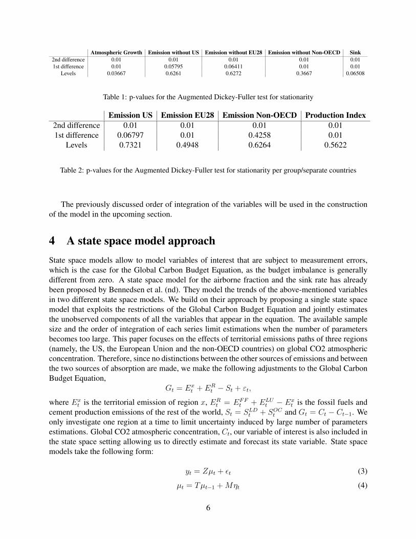
Atmospheric Growth Emission without US Emission without EU28 Emission without Non-OECD Sink2nd difference 0.01 0.01 0.01 0.01 0.011st difference 0.01 0.05795 0.06411 0.01 0.01

Levels 0.03667 0.6261 0.6272 0.3667 0.06508

Table 1: p-values for the Augmented Dickey-Fuller test for stationarity

Emission US Emission EU28 Emission Non-OECD Production Index2nd difference 0.01 0.01 0.01 0.011st difference 0.06797 0.01 0.4258 0.01

Levels 0.7321 0.4948 0.6264 0.5622

Table 2: p-values for the Augmented Dickey-Fuller test for stationarity per group/separate countries

The previously discussed order of integration of the variables will be used in the constructionof the model in the upcoming section.

4 A state space model approachState space models allow to model variables of interest that are subject to measurement errors,which is the case for the Global Carbon Budget Equation, as the budget imbalance is generallydifferent from zero. A state space model for the airborne fraction and the sink rate has alreadybeen proposed by Bennedsen et al. (nd). They model the trends of the above-mentioned variablesin two different state space models. We build on their approach by proposing a single state spacemodel that exploits the restrictions of the Global Carbon Budget Equation and jointly estimatesthe unobserved components of all the variables that appear in the equation. The available samplesize and the order of integration of each series limit estimations when the number of parametersbecomes too large. This paper focuses on the effects of territorial emissions paths of three regions(namely, the US, the European Union and the non-OECD countries) on global CO2 atmosphericconcentration. Therefore, since no distinctions between the other sources of emissions and betweenthe two sources of absorption are made, we make the following adjustments to the Global CarbonBudget Equation,

Gt = Ext + ER

t − St + εt,

where Ext is the territorial emission of region x, ER

t = EFFt + ELU

t − Ext is the fossil fuels and

cement production emissions of the rest of the world, St = SLDt + SOCt and Gt = Ct − Ct−1. Weonly investigate one region at a time to limit uncertainty induced by large number of parametersestimations. Global CO2 atmospheric concentration, Ct, our variable of interest is also included inthe state space setting allowing us to directly estimate and forecast its state variable. State spacemodels take the following form:

yt = Zµt + εt (3)

µt = Tµt−1 +Mηt (4)

6

Equation (3) represents the observation equation, that is, we observe variable y but the variableof interest is its state, µ, which is not observed. The error term in the observation equation hencerepresents the measurement error in the observed variable. The transition equation (4), representsunderlying dynamics of the variables of interest.

Global CO2 atmospheric concentration growth (Gt) can on the one hand be measured fromenvironmental models, but can also be approximated by the difference between total emissions andabsorption (Ex

t +ERt −St). That is, with different measurement errors,Gt and (Ex

t +ERt −St) should

have the same state variable in the observation equations. Following the structure of Equation (3)and the assumptions made, we extend the basic example with our set of variables, leading to thefollowing observation equations,

CtGt

ERt + Ex

t − StERt

StExt

=

1 0 0 00 1 −1 10 1 −1 10 1 0 00 0 1 00 0 0 1

µCtµRtµStµxt

+ εt, (5)

where εt is a vector stacking the six error terms of the observation equations, they are assumedindependently normally distributed with mean zero and distinct variance: εt ∼ N(0, H), H =diag(σ2

C,ε, σ2G,ε, σ

2R+x−S,ε, σ

2R,ε, σ

2S,ε, σ

2x,ε). The CO2 atmospheric concentration variable is I(2) and

its first difference is equal toGt, which is I(1) and depends on the states ofERt ,Ex

t and St which arethemselves I(1), as explained in Section 3. Hence, the state variables are assumed to be integratedof the same order as their corresponding observed variables and the transition equations of the fourstates of interest are as follows,

µCtµRtµStµxt

=

1 1 −1 10 1 0 00 0 1 00 0 0 1

µCt−1µRt−1µSt−1µxt−1

+ ηt. (6)

The four error terms ηt are also assumed independently normally distributed with mean zero anddistinct variance: ηt ∼ N(0, Q), Q = diag(σ2

C,η, σ2R,η, σ

2S,η, σ

2x,η). The matrix M from Equation

(4) is equal to the identity matrix.

The hyperparameters of the model described above, i.e., all the variances of the error terms, areestimated by maximizing the following diffuse log-likelihood,

`d = −Tn

2log(2π)− 1

2

T∑t=d+1

log (|Ft|)−1

2v′tF

−1t vt,

where d is the number of non-stationary variables, and vt and Ft are, respectively, the predictionerrors and their covariance matrix. The latter are estimated, together with the state variables andtheir covariance matrices, via the Kalman filter recursions,

7

vt = yt − ZatFt = ZPtZ

′ +H

Kt = TPtZ′F−1t

at|t = at + PtZ′F−1t vt

Pt|t = Pt − PtZ ′F−1t ZPt

at+1 = Tat +Ktvt

Pt+1 = TPt (T −KtZ)′ +Q,

with t = 1, . . . , T . We use a diffuse initialization for all the state variables, as all of them arenon-stationary (Durbin and Koopman, 2012).

5 Results

5.1 EstimationWe estimate our proposed state space model for the sample period starting in 1959 and ending in2017. Figures 1, 2 and 3 report, respectively, the filtered estimates of the state variables µCt for Ct,µRt + µxt − µSt of Gt and µxt of Ex

t , when x = US, together with their 95% confidence intervals,which are constructed using the estimates for Pt|t from the Kalman filter recursions. The figuresshow that the adequacy of the restriction on the state variable of Gt being equal to the one ofERt + Ex

t − St, as the estimated local trend, does not deviate much from the observed series Gt.On the contrary, the occasional deviations of the estimated trend from ER

t + Ext − St are due to

a deterioration of the model when imposing a common trend (Bennedsen et al., nd). We do notventure into diagnostic checking as our main interest relies on the forecast of the state variables,rather than on a correct model specification. For the same reason we do not use Kalman filteringinstead of smoothing.

5.2 Forecasts scenariosScientists have already performed several in-depth analyses of how the CO2 concentration wouldevolve when different restrictions are imposed over a forecast horizon until 2100. This set of scen-ario forecasts of the atmospheric greenhouse gas concentrations are called Representative Concen-tration Pathways (RCPs). For each category of emissions (for instance, agricultural emissions andaviation emissions), an RCP contains a set of starting values and the estimated emissions up to theyear 2100, based on assumptions about economic activity, energy sources, population growth andother socio-economic factors (Moss et al., 2010). We consider four of these pathways: RCP8.5,RCP6, RCP4.5 and RCP2.6. Table 3 specifies the details of each path. Radioactive forcing meas-ures the influence of a factor in the change of the Earth’s energy balance (in watt per square meters).The goal of working with these different scenarios is not to predict the future but to better under-stand uncertainties and alternative futures. In this way, it is easy to derive how robust differentpolitical decisions or options may be under a range of possible futures. In order to explore whatthe RCP concentration scenarios imply for our forecasted emission paths, we use the RCP dataset obtained from http://www.iiasa.ac.at/web-apps/tnt/RcpDb/. We have 82 observations, startingfrom 2019 up to 2100. Note here that the values provided in this data set are slightly lower than theones indicated for the CO2 concentration in Table 3. We are going plot the RCP CO2 concentration

8

Figure 1: In-sample estimates of the state variable µCt of Ct in GtC/yr, when x = US, together with their95% confidence intervals.

Figure 2: In-sample estimates of the state variable µRt + µxt − µSt of Gt in GtC/yr, when x = US, togetherwith their 95% confidence intervals.

paths for the four scenarios together with our forecasted series of CO2 concentration.

9

Figure 3: In-sample estimates of the state variable µxt of Ext in GtC/yr, when x = US, together with their95% confidence intervals.

Radiative CO2 TemperatureName Forcing Concentration (in ppm) Anomaly Pathway

RCP8.5 8.5 Wm2 in 2100 1370 4.9 RisingRCP6 6 Wm2 post 2100 850 3 Stabilization without overshoot

RCP4.5 4.5 Wm2 post 2100 650 2.4 Stabilization without overshootRCP2.6 3 Wm2 before 2100, 490 1.5 Peak and decline

declining to 6Wm2 2100

Table 3: RCP-Scenarios Explanation

We based our forecast evaluation on the accordingly forecasted state variables and build predic-tion intervals using the forecasted variances of the state variables. In presence of missing observa-tions, the Kalman filter is carried out by imposing Kt = 0 and vt = 0. We perform 83 recursivelyobtained one-step ahead forecasts, from 2018 to 2100. Figure 4 and 5 show the CO2 atmosphericconcentration forecast with respectively the 99% and 50% confidence intervals. Due to the signi-ficantly far horizon and the recursively dependent forecasts, the confidence intervals significantlywiden, leading to a possible CO2 atmospheric concentration in the year 2100 between 0 and 1200ppmv in 2100 at the 99% confidence interval. Furthermore, at such confidence interval, all pathsare within the possible range. Our forecast lies within RCP4.5 and RCP6, which correspondsto a maximum temperature increase of around 2.75 degrees above pre-industrial level (calibratedtemperature from Table 3). Yet, since all possible scenarios are within the confidence range, tem-perature could potentially increase to a maximum of 4.9 degrees above pre-industrial level or toonly a maximum of 1.5 degrees as depicted from the two extreme scenarios. The resulting graphs

10

when x = EU28 and non-OECD are similar and can be found in the Appendix (Figures 28 and 29).

Figure 4: Out of sample forecasts of µCt of Ct in ppmv, when x = US, together with their 99% confidenceintervals, compared to the RCP forecasted scenarios.

Reducing the confidence interval to 75% then renders unlikely the worst case scenario (RCP8.5)for all x as shown in Figures 30, 31 and 32 in the Appendix. Further decreasing the confidenceinterval to 50% leads to the additional exclusion of the best case scenario (RCP2.6) when x = USand non-OECD as shown in Figures 5 and 33. On the contrary, we see the striking result, that whenwe consider x = EU28, we still do include the best case scenario (RCP2.6) in the 50% confidenceinterval as seen in Figure 6. We see these slight differences due to the fact that we are specifyingthe state space model in a different way. The underlying principle of both models is the same, butdue to these different model specifications we can get different results. All the above results aregiven the condition that the future will follow the current trend of the growth of CO2 concentra-tions. Hence, we are quite likely to find ourselves in the medium cases if no changes are imposedon the emission pathway. This shows that in order to reach the goals of the COP21 in Paris, theneed for new climate policies becomes urgent.

5.3 Sensitivity AnalysisIn this section, we will conduct a sensitivity analysis on the CO2 concentration path for each groupof countries. Furthermore, we compare each scenario to the RCP scenarios to evaluate the impactmagnitude of different group of countries/individual countries on the temperature rise. We simulatedifferent scenarios in order to do this. In the first setting, we lower the last value of emissions ofthe group of countries/country by 0.8 GtC/yr, which corresponds to 56% reduction in emissions. In

11

Figure 5: Out of sample forecasts of µCt of Ct in ppmv, when x = US, together with their 50% confidenceintervals, compared to the RCP forecasted scenarios.

Figure 6: Out of sample forecasts of µCt of Ct in ppmv, when x = EU28, together with their 50% confidenceintervals, compared to the RCP forecasted scenarios.

the second setting, we increase it by 2 GtC/yr, which corresponds to a 139% increase in emissionsin the US. Due to the same magnitude of alteration for each country, we can now evaluate which

12

country has the highest impact and which ones do not have any impact. In this way, we can derivesuggestions for policy makers with respect to which countries we should focus on to achieve thegoals of a specified maximum temperature increase. Figure 7 and 8 as well as Figure 34- 37 in theAppendix display the future CO2 concentration path for the EU28 countries, so x = EU28. Figure9 and 10 as well as Figure 38- 41 in the Appendix depict the path for the US (x = US) and Figure 11and 12 as well as Figure 42- 45 in the Appendix for the non-OECD (x = non-OECD) countries. Werecognize that, due to the small sample size and far ahead forecast, the 99% confidence intervalis very wide for all groups and, hence, all RCP paths are within possible range. Reducing theconfidence interval to 75% already leads to different results. We observe that all groups excludethe worst case scenario. However, whereas for the EU28 countries, the exclusion is very clear andstrong, this is not the case for the US and the non-OECD countries, especially with respect to thesecond simulation where we increase the emissions. In this case, the upper bound of the confidenceinterval and the worst case scenario almost coincide. Reducing the confidence interval even moreto 50%, we can draw several more conclusions. We consider the first simulation, namely a dropby 0.8 GtC/yr, first. Here, we clearly recognize that the confidence interval is tilted towards thebest case scenario. The point estimate for year 2100 coincides with the RCP4.5 scenario, meaninga temperature increase of maximum 2.4 degrees. The worst case scenario lies far beyond theupper bound. Moreover, the second worst case scenario is very close to the upper bound. Forthe non-OECD countries and the US, the best as well as worst case scenarios are excluded fromthe confidence interval, though the best case scenario is close to the lower bound. Nonetheless,the point estimate for year 2100 is for both groups in between all RCP scenarios and correspondsto a CO2 concentration of approximately 560 ppmv, so a temperature increase of maximum 2.75degrees. Analyzing the second simulation scenario, we observe that all groups exclude the worstand best case scenario from the interval. The worst case scenario still lies quite far outside ofthe interval whereas the best scenario is relatively close to the lower bound. Overall, we see thatthe decrease of emissions in the EU28 countries has the biggest impact on the forecasted CO2concentration pathway. The confidence intervals are tilted towards the best case scenario and thepoint estimate is very close to the RCP4.5, so a maximum temperature increase of 2.4 degrees.Moreover, the worst case scenario lies far away from the upper bound of the confidence interval.The US and non-OECD countries experience similar consequences after a decrease/increase inemissions. Both groups show that an alteration of the emissions have less impact on the forecastedCO2 concentration path in comparison to the EU countries. Moreover, from the second simulatedscenario, we see that an increase in the emissions of the EU countries has less negative impactthan of the other two groups. For these, the upper bound of the 75% confidence interval almostcoincides with the worst case scenario, so it is almost included, while this is clearly not the case forthe EU countries. Hence, although the EU countries have a higher positive impact when reductionis imposed, the US and non-OECD countries have a bigger negative impact when an increase inemission takes place. This is important to keep in mind when introducing new regulations. Eventhough the impact of developing countries on global CO2 concentration may not significantly differfrom the one of developed countries, their economic activity might be harmed by policies whichaim at reducing CO2 emissions. Therefore, developed countries are urged to lean towards thesepolicies.

13

Figure 7: Out of sample forecasts of µCt of Ct in ppmv if emissions of EU dropped by 0.8 GtC/yr, togetherwith their 75% confidence intervals, compared to the RCP forecasted scenarios.

Figure 8: Out of sample forecasts of µCt of Ct in ppmv if emissions of EU increased by 2 GtC/yr, togetherwith their 75% confidence intervals, compared to the RCP forecasted scenarios.

5.4 CO2 emissions and economic activityAs mentioned by Andersson and Karpestam (2013), while there is strong consensus in scientificcommunities that rising global temperatures must be combated, there is also a concern that imple-

14

Figure 9: Out of sample forecasts of µCt of Ct in ppmv if emissions of US dropped by 0.8 GtC/yr, togetherwith their 75% confidence intervals, compared to the RCP forecasted scenarios.

Figure 10: Out of sample forecasts of µCt of Ct in ppmv if emissions of US increased by 2 GtC/yr, togetherwith their 75% confidence intervals, compared to the RCP forecasted scenarios.

menting emissions reductions too quickly will limit economic growth. In this section we focus onthe US emissions. We extend our initial model with the addition of its industrial production index

15

Figure 11: Out of sample forecasts of µCt of Ct in ppmv if emissions of Non-OECD dropped by 0.8 GtC/yr,together with their 75% confidence intervals, compared to the RCP forecasted scenarios.

Figure 12: Out of sample forecasts of µCt of Ct in ppmv if emissions of Non-OECD increased by 2 GtC/yr,together with their 75% confidence intervals, compared to the RCP forecasted scenarios.

as an indicator of US economic activity, denoted It,

16

CtGt

ERt + Ex

t − StERt

StExt

It

=

1 0 0 0 00 1 −1 1 00 1 −1 1 00 1 0 0 00 0 1 0 00 0 0 1 00 0 0 0 1

µCtµRtµStµxtµIt

+ εt, (7)

where εt is a vector stacking the seven error terms of the observation equations, they are assumedindependently normally distributed with mean zero and distinct variance: εt ∼ N(0, H), H =diag(σ2

C,ε, σ2G,ε, σ

2R+x−S,ε, σ

2R,ε, σ

2S,ε, σ

2x,ε, σ

2I,ε). The transition equations are then as follows,

µCtµRtµStµxtµIt

=

1 1 −1 1 00 1 0 0 00 0 1 0 00 0 0 1 00 0 0 0 1

µCt−1µRt−1µSt−1µxt−1µIt−1

+ ηt. (8)

What changes in this model is that we assume that the error terms of the state variables of µxtand µIt are correlated. Hence, ηt ∼ N(0, Q), where

Q =

σ2C,η 0 0 0 00 σ2

R,η 0 0 00 0 σ2

S,η 0 00 0 0 σ2

x,η ρσI,ησx,η0 0 0 ρσI,ησx,η σ2

I,η

.As such, it implies that the conditional expectation of US emissions will depend on its own pastvalue but also on the contemporary change of the economic activity,

E[µxt+1|µxt , µIt+1] = µxt + ρσx,ησI,η

(µIt+1 − µIt ). (9)

Intuitively, an increase in production, given a state of technology and other factors, should increaseemissions.

In Section 5.3, we investigated the effect of a change in emissions on CO2 concentrations. Wehence just fix future emission paths and performed forecasts of levels of concentrations. We nowinvestigate the means for such reduction in CO2 emissions. As just mentioned we assume thatemissions are driven by changes in production, we hence investigate the sensitivity of US CO2emissions to variations in production.

The hyperparameters of the model are estimated in the same way as in Section 4, yielding anestimated correlation of ρ = 0.59. We then perform similar sensitivity analyses by imposing futurepaths of economic activity. We consider two scenarios. The first one corresponds to a permanentdecrease of 20% in production and the forecast of US CO2 emissions is depicted in Figure 13. Asexpected from the conditional expectation depicted in Equation (9), the forecast of emissions falls

17

by roughly 62% as the production drops by 20% and then is remains constant. The 62% decreasein US emissions is roughly equal to the decrease of 0.8 GtC simulated in Section 5.3. This sig-nals that CO2 emissions responds with a magnitude 3 times higher than the shock in production.Yet, such a cut in production is rather drastic. Instead, we consider a second scenario in whichproduction gradually decrease by 2.5% a year, corresponding to the same decrease in emissionsby 2100. Figure 14 shows the forecast over the next 83 years of US CO2 emissions with suchscenario. The scenario, more realistic, indicates that by gradually decreasing production by 2.5%a year, emissions will already be reduced by a half in 2040.

Figure 13: Out of sample forecasts of µXt of Ext in GtC/y, when x = US, assuming a permanent decrease of20% in production for the out-of sample period.

The results in this section suggests that emissions reduction, at least in the US, do not requiresuch significant decrease in production, as feared. Emissions in the US could, as this model indic-ates, be reduced by half by 2040 if production was gradually decreased by 2.5% a year. Of course,this section assumes all other factors constant, as well as no technological progress. Technolo-gical progress and the expansion of renewable energy allows production to increase while havingdecreasing emissions. On the other hand, territorial emissions could be reduced while keeping pro-duction constant if offshoring is performed in developing countries where climate regulations aremore lenient. Via such process, territorial emissions indeed decrease but global emissions remainunchanged.

18

Figure 14: Out of sample forecasts of µXt of Ext in GtC/y, when x = US, assuming a decrease of 2.5% peryear in production.

6 DiscussionA key motivation to undertake this study has been to model CO2 atmospheric concentration usingan econometric approach. The basis of our model is the Global Carbon Budget Equation and by us-ing a state-space approach we intend to tackle the measurement errors that climate data are subjectto. Following the critiques of Friedlingstein (2015) and Bennedsen et al. (nd), we do recognize thata drawback of the constructed model is that it does not incorporate the carbon-climate feedback.Since the discussion of these effects are still heated, we do realize that it is worth while to expandthe model and include these effects. Therefore, we suggest this for further research, following theidea of coupled carbon-climate models.

Moreover, due to having only yearly data at hand, the sample size is relatively small (59 datapoints). Hence, drawing reliable conclusions is very hard and limited, e.g. tests like the ADF-testmay not be valid. We also acknowledge this problem in the forecasts. Predicting more than 80out-of-sample forecasts with a model that is estimated using less than 60 observations leads tosubstantial uncertainty, especially the further in the future the forecasts are.

A third limitation is the number of variables used in the model. We decided to merge therest of the world’s emissions with the global land-use change emissions and also merged the twosink variables to reduce the dimensionality. In this way, we cannot distinguish the emissions andsinks and cannot draw individual conclusions. Additionally, we limited our data set to those 6or 7 variables while potentially other external factors could influence CO2 concentration, such asthe direct, or indirect effects of other greenhouse gas, population growth or technological progress

19

for instance. Furthermore, while looking at the effects of changes in production on the US CO2emissions, even more external factors may be affecting the link between the two variables, such asoffshoring factories as explained in the previous part.

Another major shortcoming arises in the model specification for the impact of different regions.Here, we evaluate individual models for each region instead of modelling them together. This ismainly due to the small sample size. We cannot estimate all these parameters given the few datapoints. In this way, we can only check which group of countries have a higher impact on the evol-ution of the CO2 concentration path, but we cannot investigate the different future paths if we altereach of the regions differently, e.g. in a first scenario reduce emissions significantly in the US andonly slightly in the EU28 countries and in a second scenario vice versa.

Another limitation arises in the sensitivity analysis, where we set the value of emissions equalto the last value plus or minus a specific amount and then keep it constant in the model. This isdone in order to then evaluate the path of the carbon concentration after a policy intervention forexample. However, this is not realistic due to two reasons. First of all, it is assumed that the valueof emissions will stay constant over time. This is highly unlikely. Second, the model currentlyassumes a big jump in the value of emissions at the beginning to investigate the different scenarios.An extension of this simulation study would be to let the values gradually increase/decrease at aspecific rate over time, hence find a decreasing time series of emissions such that the value of C2100

is equal to the desired value depending on which scenario we are investigating.

To put it in a nutshell, the model constructed in this paper is rather simplified and may lackdynamics or external factors. However, it tackles the problem of measurement errors, it is basedon the Carbon Budget Equation, and its forecasts in are line with climate specialists scenariosforecasts. We investigate individual effects of changes in three regions’ CO2 emissions and theeffect of a drop in production on CO2 emissions in the US. Yet, further research could extend theconstructed state space model to incorporate the effect of countries combined.

7 ConclusionClimate change is nowadays a key topic of interest in political discussions. It is crucial to haveproper models and perform accurate forecasts of climate-related variables to efficiently tackle theissues that climate change brings. In order to introduce new policies, it is important not only toclearly identify the impact of separate groups of countries but also to evaluate the consequencesof such policies on economic activity for instance. This gave rise to multidisciplinary approaches,such as the use of econometric methods to model climate series and their dynamics. This paper fo-cuses on measuring the impact of changes in CO2 emissions in different regions of the world on theatmospheric concentration and then investigates by what means such reductions can be achievedwith the example of the US.

We propose a state space approach that takes into account the measurement errors to whichclimate data are subject. This was motivated by the persistent Global Carbon Budget Equationimbalance observed in practice over the past years. The model is based on this equation and allows

20

to jointly estimate and forecast all the unobserved components driving the observed variables ofthe Budget Equation and CO2 concentrations. Our analysis provides insights into a distributionscheme for the emission reductions across groups of countries in order to reach goals set duringclimate summits, such as the maximum of 2 degrees rise above pre-industrial levels set by theCOP21, and further explores the consequences of these schemes on economic activity.

We compare our forecast of CO2 concentration from 2018 to 2100 to Representative Concen-tration Pathways that correspond to distinct scenarios leading to different temperature increasesabove pre-industrial levels. We find that if all variables follow the current trend, any scenario froma maximum increase of 1.5 degrees above pre-industrial level to a maximum increase of 4.9 de-grees lies within the 99% confidence interval for all three regions considered. Even though theworst case scenario is excluded in all of the 50% confidence intervals, so is the best case scenarioin most of the models, which corresponds to a maximum increase of 1.5 degrees.

We perform a sensitivity analysis by imposing future emission paths of specific countries andinvestigate their effect on potential future temperature rise under RCP scenarios. Further, we com-pare the magnitude of the impact among three regions, the US, the EU28 and the non-OECD coun-tries. We find that if emissions of one group of countries are altered and all other variables followcurrent trends, any scenario from a maximum increase of 1.5 degrees above pre-industrial level toa maximum increase of 4.9 degrees lies within the 99% confidence interval. Further, reducing theconfidence intervals to 75% and 50%, we can conclude that the confidence intervals for the EU28countries is tilted towards the best case scenario in a reduction of emissions and the worst casescenario lies far outside of the interval. For the US and non-OECD countries, on the contrary, wefind that the best case scenario is sometimes even excluded from the confidence interval. Overall,we do see a little shift towards the best case scenario for each region. Hence, combined this canlead to an achievement of the goals set. While we do not find significant difference in the effectsof changes in CO2 emissions between developed and developing countries, the fact is developingcountries activity may be severely harmed by policies intending to reduce emissions. Hence, eventhough their impact on global CO2 concentration may be the same, they cannot be asked to havepolicies of the same magnitude as developed countries.

We then investigate how a decrease in CO2 emissions could actually be achieved in the casefor the US. We assumed that CO2 emissions are affected by changes in production. We find thatin the US, CO2 emissions react to changes in production with a magnitude 3 times higher thanthe actual change in the production. While people fear that decreasing emissions may significantlyharm economic activity, our model indicates that by gradually decreasing production by 2.5% ayear, CO2 emissions could be reduced by a half by 2040. We did not take into account variousexternal factors that may affect the relationship between the two variables, and leave that for furtherresearch.

21

ReferencesAndersson, F. N. and Karpestam, P. (2013). Co2 emissions and economic activity: Short-and long-

run economic determinants of scale, energy intensity and carbon intensity. Energy Policy,61:1285–1294.

Ballantyne, A. P., Andres, R., Houghton, R., Stocker, B. D., Wanninkhof, R., Anderegg, W.,Cooper, L. A., DeGrandpre, M., Tans, P. P., Miller, J. B., Alden, C., and White, J. W. C.(2015). Audit of the global carbon budget: estimate errors and their impact on uptake uncer-tainty. Biogeosciences, 12(8):2565–2584.

Bennedsen, M., Hillebrand, E., and Koopman, S. J. (n.d.). Trend analysis of the airborne fractionand sink rate of anthropogenically released co2.

Canadell, J., Ciais, P., Gurney, K., Le Quere, C., Piao, S., Raupach, M., and Sabine, C. (2011). Aninternational effort to quantify regional carbon fluxes. Eos, 92(10):81–82.

Clemencon, R. (2016). The two sides of the paris climate agreement: Dismal failure or historicbreakthrough?

Durbin, J. and Koopman, S. J. (2012). Time series analysis by state space methods. Oxforduniversity press.

Friedlingstein, P. (2015). Carbon cycle feedbacks and future climate change. PhilosophicalTransactions of the Royal Society A: Mathematical, Physical and Engineering Sciences,373(2054):20140421.

Gloor, M., Sarmiento, J. L., and Gruber, N. (2010). What can be learned about carbon cycleclimate feedbacks from the co 2 airborne fraction? Atmospheric Chemistry and Physics,10(16):7739–7751.

Le Quere, C., Andrew, R. M., Friedlingstein, P., Sitch, S., Hauck, J., Pongratz, J., Pickers, P. A.,Korsbakken, J. I., Peters, G. P., Canadell, J. G., Arneth, A., Arora, V. K., Barbero, L., Bastos,A., Bopp, L., Chevallier, F., Chini, L. P., Ciais, P., Doney, S. C., Gkritzalis, T., Goll, D. S.,Harris, I., Haverd, V., Hoffman, F. M., Hoppema, M., Houghton, R. A., Hurtt, G., Ilyina,T., Jain, A. K., Johannessen, T., Jones, C. D., Kato, E., Keeling, R. F., Goldewijk, K. K.,Landschutzer, P., Lefevre, N., Lienert, S., Liu, Z., Lombardozzi, D., Metzl, N., Munro, D. R.,Nabel, J. E. M. S., Nakaoka, S.-I., Neill, C., Olsen, A., Ono, T., Patra, P., Peregon, A., Peters,W., Peylin, P., Pfeil, B., Pierrot, D., Poulter, B., Rehder, G., Resplandy, L., Robertson, E.,Rocher, M., Rodenbeck, C., Schuster, U., Schwinger, J., Seferian, R., Skjelvan, I., Steinhoff,T., Sutton, A., Tans, P. P., Tian, H., Tilbrook, B., Tubiello, F. N., van der Laan-Luijkx, I. T.,van der Werf, G. R., Viovy, N., Walker, A. P., Wiltshire, A. J., Wright, R., Zaehle, S., andZheng, B. (2018). Global carbon budget 2018. Earth System Science Data, 10(4):2141–2194.

Moss, R. H., Edmonds, J. A., Hibbard, K. A., Manning, M. R., Rose, S. K., Van Vuuren, D. P.,Carter, T. R., Emori, S., Kainuma, M., Kram, T., et al. (2010). The next generation of scenariosfor climate change research and assessment. Nature, 463(7282):747.

22

Strassmann, K. M. and Joos, F. (2018). The bern simple climate model (bernscm) v1. 0: an extens-ible and fully documented open-source re-implementation of the bern reduced-form modelfor global carbon cycle–climate simulations. Geoscientific Model Development, 11(5):1887–1908.

23

Appendices

Atmospheric Growth Emission without US Emission without EU Emission without Non-OECD SinkMean 3.258692 5.957751 6.193513 4.509751 3.88693

Standard Deviation 1.381219 1.92756 2.101062 0.6317307 1.41866

Table 4: Summary Statistics

Emission US Emission EU Emission Non-OECD Production IndexMean 1.323834 1.088072 2.771834 65.62633

Standard Deviation 0.2534717 0.1417442 1.544902 26.58313

Table 5: Summary Statistics

(a) Sink Level (b) Sink First Difference

Figure 15: Sink

(a) Atmospheric Growth Level(b) Atmospheric Growth First Dif-ference

Figure 16: Atmospheric Growth

24

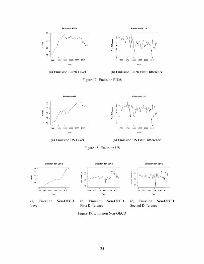
(a) Emission EU28 Level (b) Emission EU28 First Difference

Figure 17: Emission EU28

(a) Emission US Level (b) Emission US First Difference

Figure 18: Emission US

(a) Emission Non-OECDLevel

(b) Emission Non-OECDFirst Difference

(c) Emission Non-OECDSecond Difference

Figure 19: Emission Non-OECD

25

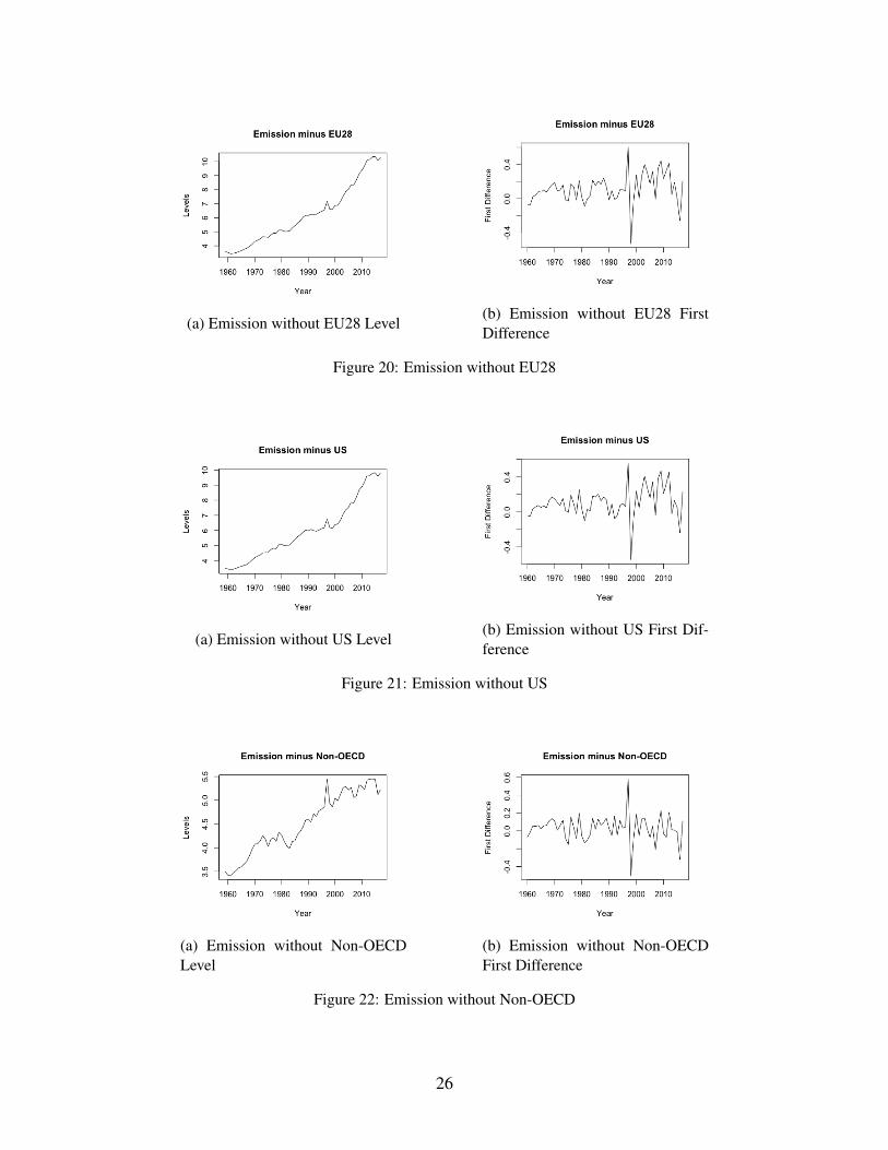
(a) Emission without EU28 Level(b) Emission without EU28 FirstDifference

Figure 20: Emission without EU28

(a) Emission without US Level(b) Emission without US First Dif-ference

Figure 21: Emission without US

(a) Emission without Non-OECDLevel

(b) Emission without Non-OECDFirst Difference

Figure 22: Emission without Non-OECD

26

(a) Production Index Level(b) Production Index First Differ-ence

Figure 23: Industrial Production Index US

Figure 24: In-sample estimates of the state variable µCt of Ct in GtC/yr, when x = EU28, together with their95% confidence intervals.

27

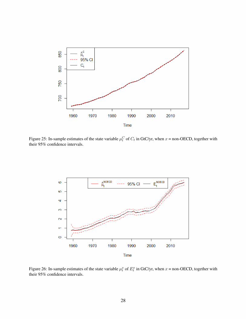
Figure 25: In-sample estimates of the state variable µCt of Ct in GtC/yr, when x = non-OECD, together withtheir 95% confidence intervals.

Figure 26: In-sample estimates of the state variable µxt of Ext in GtC/yr, when x = non-OECD, together withtheir 95% confidence intervals.

28

Figure 27: In-sample estimates of the state variable µxt of Ext , when x = EU28 in GtC/yr, together with their95% confidence intervals.

Figure 28: Out of sample forecasts of µCt ofCt in ppmv, when x = EU28, together with their 99% confidenceintervals, compared to the RCP forecasted scenarios.

29

Figure 29: Out of sample forecasts of µCt of Ct in ppmv, when x = non-OECD, together with their 99%confidence intervals, compared to the RCP forecasted scenarios.

Figure 30: Out of sample forecasts of µCt ofCt in ppmv, when x = EU28, together with their 75% confidenceintervals, compared to the RCP forecasted scenarios.

30

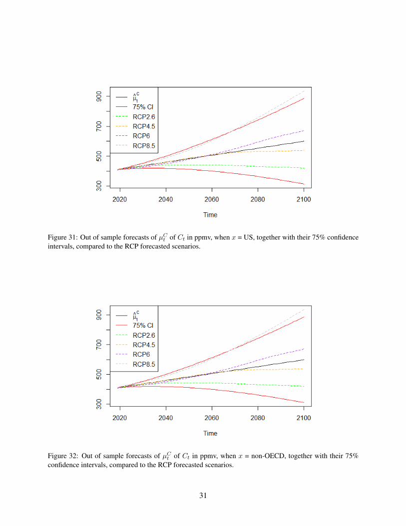
Figure 31: Out of sample forecasts of µCt of Ct in ppmv, when x = US, together with their 75% confidenceintervals, compared to the RCP forecasted scenarios.

Figure 32: Out of sample forecasts of µCt of Ct in ppmv, when x = non-OECD, together with their 75%confidence intervals, compared to the RCP forecasted scenarios.

31

Figure 33: Out of sample forecasts of µCt of Ct in ppmv, when x = non-OECD, together with their 50%confidence intervals, compared to the RCP forecasted scenarios.

Figure 34: Out of sample forecasts of µCt ofCt in ppmv if emissions of EU28 dropped by 0.8 GtC/y, togetherwith their 50% confidence intervals, compared to the RCP forecasted scenarios.

32

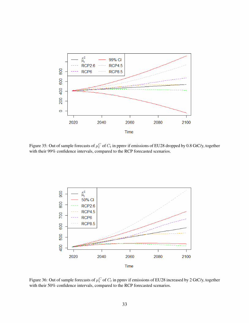
Figure 35: Out of sample forecasts of µCt ofCt in ppmv if emissions of EU28 dropped by 0.8 GtC/y, togetherwith their 99% confidence intervals, compared to the RCP forecasted scenarios.

Figure 36: Out of sample forecasts of µCt ofCt in ppmv if emissions of EU28 increased by 2 GtC/y, togetherwith their 50% confidence intervals, compared to the RCP forecasted scenarios.

33

Figure 37: Out of sample forecasts of µCt ofCt in ppmv if emissions of EU28 increased by 2 GtC/y, togetherwith their 99% confidence intervals, compared to the RCP forecasted scenarios.

Figure 38: Out of sample forecasts of µCt of Ct in ppmv if emissions of US dropped by 0.8 GtC/y, togetherwith their 50% confidence intervals, compared to the RCP forecasted scenarios.

34

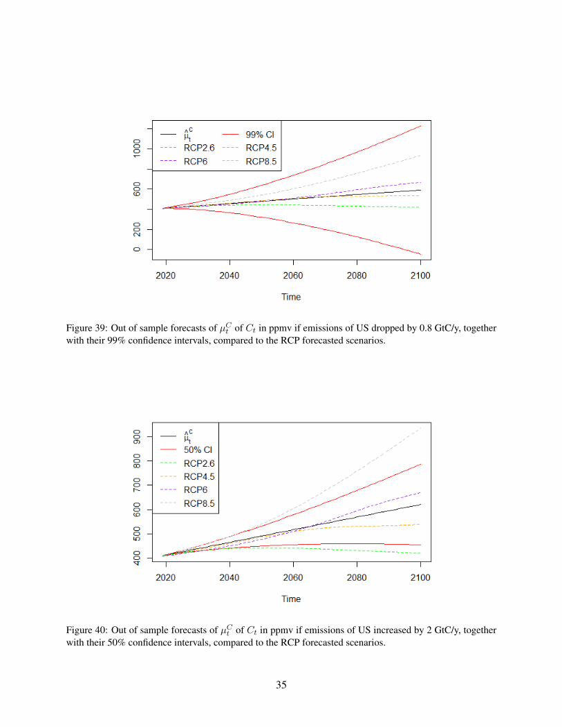
Figure 39: Out of sample forecasts of µCt of Ct in ppmv if emissions of US dropped by 0.8 GtC/y, togetherwith their 99% confidence intervals, compared to the RCP forecasted scenarios.

Figure 40: Out of sample forecasts of µCt of Ct in ppmv if emissions of US increased by 2 GtC/y, togetherwith their 50% confidence intervals, compared to the RCP forecasted scenarios.

35

Figure 41: Out of sample forecasts of µCt of Ct in ppmv if emissions of US increased by 2 GtC/y, togetherwith their 99% confidence intervals, compared to the RCP forecasted scenarios.

Figure 42: Out of sample forecasts of µCt of Ct in ppmv if emissions of Non-OECD dropped by 0.8 GtC/y,together with their 50% confidence intervals, compared to the RCP forecasted scenarios.

36

Figure 43: Out of sample forecasts of µCt of Ct in ppmv if emissions of Non-OECD dropped by 0.8 GtC/y,together with their 99% confidence intervals, compared to the RCP forecasted scenarios.

Figure 44: Out of sample forecasts of µCt of Ct in ppmv if emissions of Non-OECD increased by 2 GtC/y,together with their 50% confidence intervals, compared to the RCP forecasted scenarios.

37

Figure 45: Out of sample forecasts of µCt of Ct in ppmv if emissions of Non-OECD increased by 2 GtC/y,together with their 99% confidence intervals, compared to the RCP forecasted scenarios.

38